agency seattle wa 96101 washington a review and …

EPA 910-R-99-010 Alaska

United States Region 10 Idaho

Environmental Protection 1200 Sixth Avenue Oregon

Agency Seattle WA 96101 Washington

Water Division Water Resources Assessment July 1999

A Review and Synthesis of Effects of Alterations to the Water Temperature Regime on Freshwater Life Stages of Salmonids, with Special Reference to Chinook Salmon

A REVIEW AND SYNTHESIS OF EFFECTS OF ALTERATIONS TO THE WATERTEMPERATURE REGIME ON FRESHWATER LIFE STAGES OF SALMONIDS,

WITH SPECIAL REFERENCE TO CHINOOK SALMON

Prepared for the U.S. Environmental Protection AgencyRegion 10, Seattle, Washington

Contract Officer, Donald Martin, Boise, IdahoPublished as EPA 910-R-99-010, July 1999

by Dale A. McCullough, Ph.D.Columbia River Inter-Tribal Fish Commission

729 NE Oregon StreetSuite 200

Portland, OR 97232

completed February 22, 1999

TABLE OF CONTENTS

ACKNOWLDGEMENTS . . . . . . . . . . . . . . . . . . . . . . . . . . . . . . . . . . . . . . . . . . . . . vi

LIST OF FIGURES . . . . . . . . . . . . . . . . . . . . . . . . . . . . . . . . . . . . . . . . . . . . . . . . . vii

LIST OF TABLES . . . . . . . . . . . . . . . . . . . . . . . . . . . . . . . . . . . . . . . . . . . . . . . . . . ix

INTRODUCTION . . . . . . . . . . . . . . . . . . . . . . . . . . . . . . . . . . . . . . . . . . . . . . . . . . 1SALMON STATUS . . . . . . . . . . . . . . . . . . . . . . . . . . . . . . . . . . . . . . . . . . . . 1SALMON HABITAT STATUS . . . . . . . . . . . . . . . . . . . . . . . . . . . . . . . . . . . . 2POTENTIAL FOR RECOVERY. . . . . . . . . . . . . . . . . . . . . . . . . . . . . . . . . . . 5OBJECTIVES AND APPROACH TO BE TAKEN IN LITERATURE

REVIEW AND SYNTHESIS . . . . . . . . . . . . . . . . . . . . . . . . . . . . . . . . 7

TERMINOLOGY . . . . . . . . . . . . . . . . . . . . . . . . . . . . . . . . . . . . . . . . . . . . . . . . . . 10THERMAL STRESS . . . . . . . . . . . . . . . . . . . . . . . . . . . . . . . . . . . . . . . . . 10TEMPERATURE RANGES . . . . . . . . . . . . . . . . . . . . . . . . . . . . . . . . . . . . 10INCIPIENT LETHAL TEMPERATURE VS.

CRITICAL THERMAL MAXIMUM . . . . . . . . . . . . . . . . . . . . . . . . . . 13GROWTH ZONE . . . . . . . . . . . . . . . . . . . . . . . . . . . . . . . . . . . . . . . . . . . . 15PHYSIOLOGICAL OPTIMUM TEMPERATURE. . . . . . . . . . . . . . . . . . . . . . 16PRODUCTION . . . . . . . . . . . . . . . . . . . . . . . . . . . . . . . . . . . . . . . . . . . . . . 17TEMPERATURE REGIME . . . . . . . . . . . . . . . . . . . . . . . . . . . . . . . . . . . . . 17

EGG/ALEVIN LIFE STAGE. . . . . . . . . . . . . . . . . . . . . . . . . . . . . . . . . . . . . . . . . . 19CHINOOK . . . . . . . . . . . . . . . . . . . . . . . . . . . . . . . . . . . . . . . . . . . . . . . . . 19

Constant Temperature. . . . . . . . . . . . . . . . . . . . . . . . . . . . . . . . . . . . . 19Survival . . . . . . . . . . . . . . . . . . . . . . . . . . . . . . . . . . . . . . . . . 19Growth and Development. . . . . . . . . . . . . . . . . . . . . . . . . . . . . 20

Varying Temperature. . . . . . . . . . . . . . . . . . . . . . . . . . . . . . . . . . . . . 22Survival . . . . . . . . . . . . . . . . . . . . . . . . . . . . . . . . . . . . . . . . . 22Growth and Development. . . . . . . . . . . . . . . . . . . . . . . . . . . . . 24

ASSOCIATED COLDWATER SPECIES. . . . . . . . . . . . . . . . . . . . . . . . . . . . 27Constant Temperature. . . . . . . . . . . . . . . . . . . . . . . . . . . . . . . . . . . . . 27

Survival . . . . . . . . . . . . . . . . . . . . . . . . . . . . . . . . . . . . . . . . . 27UILT experiments . . . . . . . . . . . . . . . . . . . . . . . . . . . . . 28Thermal shock . . . . . . . . . . . . . . . . . . . . . . . . . . . . . . . 32

Growth and Development. . . . . . . . . . . . . . . . . . . . . . . . . . . . . 32Varying Temperature. . . . . . . . . . . . . . . . . . . . . . . . . . . . . . . . . . . . . 35

Survival . . . . . . . . . . . . . . . . . . . . . . . . . . . . . . . . . . . . . . . . . 35Growth and Development. . . . . . . . . . . . . . . . . . . . . . . . . . . . . 38

i

JUVENILE LIFE STAGE: FRY, FINGERLING, PARR. . . . . . . . . . . . . . . . . . . . . . 41CHINOOK . . . . . . . . . . . . . . . . . . . . . . . . . . . . . . . . . . . . . . . . . . . . . . . . . 41

Constant Temperature . . . . . . . . . . . . . . . . . . . . . . . . . . . . . . . . . . . . 41Survival . . . . . . . . . . . . . . . . . . . . . . . . . . . . . . . . . . . . . . . . . 41

UILT experiments . . . . . . . . . . . . . . . . . . . . . . . . . . . . . 41Thermal shock . . . . . . . . . . . . . . . . . . . . . . . . . . . . . . . 43

Growth and Development. . . . . . . . . . . . . . . . . . . . . . . . . . . . . 44Feeding . . . . . . . . . . . . . . . . . . . . . . . . . . . . . . . . . . . . . . . . . 45

Varying Temperature. . . . . . . . . . . . . . . . . . . . . . . . . . . . . . . . . . . . . 45Survival . . . . . . . . . . . . . . . . . . . . . . . . . . . . . . . . . . . . . . . . . 46

Diel cycle: . . . . . . . . . . . . . . . . . . . . . . . . . . . . . . . . . . 46Growth and Development. . . . . . . . . . . . . . . . . . . . . . . . . . . . . 46Feeding . . . . . . . . . . . . . . . . . . . . . . . . . . . . . . . . . . . . . . . . . 46

ASSOCIATED COLDWATER SPECIES. . . . . . . . . . . . . . . . . . . . . . . . . . . . 47Constant Temperature . . . . . . . . . . . . . . . . . . . . . . . . . . . . . . . . . . . . 47

Survival . . . . . . . . . . . . . . . . . . . . . . . . . . . . . . . . . . . . . . . . . 47UILT experiments: . . . . . . . . . . . . . . . . . . . . . . . . . . . . 47Thermal shock . . . . . . . . . . . . . . . . . . . . . . . . . . . . . . . 49

Growth and Development. . . . . . . . . . . . . . . . . . . . . . . . . . . . . 51Feeding . . . . . . . . . . . . . . . . . . . . . . . . . . . . . . . . . . . . . . . . . 51

Varying Temperature. . . . . . . . . . . . . . . . . . . . . . . . . . . . . . . . . . . . . 52Survival . . . . . . . . . . . . . . . . . . . . . . . . . . . . . . . . . . . . . . . . . 52

CTM experiments:. . . . . . . . . . . . . . . . . . . . . . . . . . . . . 52Stepped variation (daily). . . . . . . . . . . . . . . . . . . . . . . . 56Diel cycle: . . . . . . . . . . . . . . . . . . . . . . . . . . . . . . . . . . 56

Growth and Development. . . . . . . . . . . . . . . . . . . . . . . . . . . . . 61Diel cycles: Laboratory Evidence. . . . . . . . . . . . . . . . . . 61Diel cycles: Field Evidence. . . . . . . . . . . . . . . . . . . . . . 64Effect of Seasonal Temperature Trends. . . . . . . . . . . . . . 66

Feeding . . . . . . . . . . . . . . . . . . . . . . . . . . . . . . . . . . . . . . . . . 67Increasing Diel Temperature. . . . . . . . . . . . . . . . . . . . . . 67Diel cycles: Field Evidence. . . . . . . . . . . . . . . . . . . . . . 67

SMOLT LIFE STAGE . . . . . . . . . . . . . . . . . . . . . . . . . . . . . . . . . . . . . . . . . . . . . . 68SMOLTIFICATION IN SALMONIDS . . . . . . . . . . . . . . . . . . . . . . . . . . . . . 68

ADULT LIFE STAGE . . . . . . . . . . . . . . . . . . . . . . . . . . . . . . . . . . . . . . . . . . . . . . 73CHINOOK . . . . . . . . . . . . . . . . . . . . . . . . . . . . . . . . . . . . . . . . . . . . . . . . . 73

Constant Temperature. . . . . . . . . . . . . . . . . . . . . . . . . . . . . . . . . . . . . 73Migration or Holding Survival . . . . . . . . . . . . . . . . . . . . . . . . . 73

Varying Temperature. . . . . . . . . . . . . . . . . . . . . . . . . . . . . . . . . . . . . 74Migration: timing, normal migration temperatures, delay. . . . . . . 74Migration survival . . . . . . . . . . . . . . . . . . . . . . . . . . . . . . . . . . 76Holding . . . . . . . . . . . . . . . . . . . . . . . . . . . . . . . . . . . . . . . . . 77

ii

Spawning . . . . . . . . . . . . . . . . . . . . . . . . . . . . . . . . . . . . . . . . 78ASSOCIATED COLDWATER SPECIES. . . . . . . . . . . . . . . . . . . . . . . . . . . . 81

Constant Temperature. . . . . . . . . . . . . . . . . . . . . . . . . . . . . . . . . . . . . 81Rearing:Preference . . . . . . . . . . . . . . . . . . . . . . . . . . . . . . . . 81Migration or holding survival . . . . . . . . . . . . . . . . . . . . . . . . . . 81Spawning . . . . . . . . . . . . . . . . . . . . . . . . . . . . . . . . . . . . . . . 81

Varying Temperature . . . . . . . . . . . . . . . . . . . . . . . . . . . . . . . . . . . . 82Global and Regional Effects on Production. . . . . . . . . . . . . . . . . 82Migration: timing, normal migration temperatures, delay:. . . . . . . 83Holding . . . . . . . . . . . . . . . . . . . . . . . . . . . . . . . . . . . . . . . . . 83Rearing: Preference. . . . . . . . . . . . . . . . . . . . . . . . . . . . . . . . . 84Spawning . . . . . . . . . . . . . . . . . . . . . . . . . . . . . . . . . . . . . . . . 84Feeding . . . . . . . . . . . . . . . . . . . . . . . . . . . . . . . . . . . . . . . . . 85

Diel cycles: Laboratory Evidence. . . . . . . . . . . . . . . . . . 85Growth and Development. . . . . . . . . . . . . . . . . . . . . . . . . . . . . 86

Diel cycles . . . . . . . . . . . . . . . . . . . . . . . . . . . . . . . . . . 86Effect of Seasonal Temperature Trends. . . . . . . . . . . . . . 86

DISTRIBUTION RELATIVE TO TEMPERATURE . . . . . . . . . . . . . . . . . . . . . . . . . 87PROBLEMS IN WEIGHING THE EVIDENCE FROM LABORATORY AND

FIELD . . . . . . . . . . . . . . . . . . . . . . . . . . . . . . . . . . . . . . . . . . . . . . . 87CHINOOK . . . . . . . . . . . . . . . . . . . . . . . . . . . . . . . . . . . . . . . . . . . . . . . . . 88

Juveniles . . . . . . . . . . . . . . . . . . . . . . . . . . . . . . . . . . . . . . . . . . . . . 88Presence/Absence . . . . . . . . . . . . . . . . . . . . . . . . . . . . . . . . . 88Density . . . . . . . . . . . . . . . . . . . . . . . . . . . . . . . . . . . . . . . . 90

Adults . . . . . . . . . . . . . . . . . . . . . . . . . . . . . . . . . . . . . . . . . . . . . . 90ASSOCIATED SPECIES. . . . . . . . . . . . . . . . . . . . . . . . . . . . . . . . . . . . . . . 92

Juveniles . . . . . . . . . . . . . . . . . . . . . . . . . . . . . . . . . . . . . . . . . . . . . 92Presence/Absence. . . . . . . . . . . . . . . . . . . . . . . . . . . . . . . . . . 92Density . . . . . . . . . . . . . . . . . . . . . . . . . . . . . . . . . . . . . . . . . 95

Adults . . . . . . . . . . . . . . . . . . . . . . . . . . . . . . . . . . . . . . . . . . . . . . . 96Presence/Absence . . . . . . . . . . . . . . . . . . . . . . . . . . . . . . . . . 96Density . . . . . . . . . . . . . . . . . . . . . . . . . . . . . . . . . . . . . . . . . 96

SYNTHESIS OF DISTRIBUTION DATA . . . . . . . . . . . . . . . . . . . . . . . . . . . 97TEMPERATURE PREFERENCES OF SALMONIDS. . . . . . . . . . . . . . . . . . . 97

JUVENILE MIGRATION AND DISPERSAL . . . . . . . . . . . . . . . . . . . . . . . . . . . . . . 101CHINOOK . . . . . . . . . . . . . . . . . . . . . . . . . . . . . . . . . . . . . . . . . . . . . . . . . 101ASSOCIATED SPECIES. . . . . . . . . . . . . . . . . . . . . . . . . . . . . . . . . . . . . . . 102

DISEASE . . . . . . . . . . . . . . . . . . . . . . . . . . . . . . . . . . . . . . . . . . . . . . . . . . . . . . . 104OVERVIEW OF COMMON FRESHWATER DISEASES. . . . . . . . . . . . . . . . 104FIELD OBSERVATIONS. . . . . . . . . . . . . . . . . . . . . . . . . . . . . . . . . . . . . . . 105

Chinook . . . . . . . . . . . . . . . . . . . . . . . . . . . . . . . . . . . . . . . . . . . . . . 105

iii

Associated Species. . . . . . . . . . . . . . . . . . . . . . . . . . . . . . . . . . . . . . . 107LABORATORY OBSERVATIONS . . . . . . . . . . . . . . . . . . . . . . . . . . . . . . . . 109

Chinook . . . . . . . . . . . . . . . . . . . . . . . . . . . . . . . . . . . . . . . . . . . . . . 109Associated Species. . . . . . . . . . . . . . . . . . . . . . . . . . . . . . . . . . . . . . . 111

GENETIC VARIATION IN RESPONSE TO THERMAL ENVIRONMENT . . . . . . . . . . . . . . . . . . . . . . . . . . . . . . . . . 117FAMILY-LEVEL VARIATION . . . . . . . . . . . . . . . . . . . . . . . . . . . . . . . . . . 117

Juvenile Survival and Preference. . . . . . . . . . . . . . . . . . . . . . . . . . . . . 117SPECIES-LEVEL VARIATION . . . . . . . . . . . . . . . . . . . . . . . . . . . . . . . . . . 120

Egg/Alevin Survival and Development. . . . . . . . . . . . . . . . . . . . . . . . . 120Juvenile Survival and Preference. . . . . . . . . . . . . . . . . . . . . . . . . . . . . 122Juvenile Growth . . . . . . . . . . . . . . . . . . . . . . . . . . . . . . . . . . . . . . . . 125

STOCK-LEVEL VARIATION . . . . . . . . . . . . . . . . . . . . . . . . . . . . . . . . . . . 125Egg/Alevin Survival and Development. . . . . . . . . . . . . . . . . . . . . . . . . 125Juvenile Survival and Preference. . . . . . . . . . . . . . . . . . . . . . . . . . . . . 131Juvenile Growth . . . . . . . . . . . . . . . . . . . . . . . . . . . . . . . . . . . . . . . . 134

FAMILY GROUP VARIATION WITHIN STOCKS . . . . . . . . . . . . . . . . . . . . 136Egg/Alevin Survival and Development. . . . . . . . . . . . . . . . . . . . . . . . . 136Juvenile Survival and Preference. . . . . . . . . . . . . . . . . . . . . . . . . . . . . 138Juvenile Growth . . . . . . . . . . . . . . . . . . . . . . . . . . . . . . . . . . . . . . . . 138

CONCLUSION FROM SURVEY OF GENETIC VARIATION. . . . . . . . . . . . . 139

BIOENERGETIC CONSIDERATIONSSCOPE FOR ACTIVITY . . . . . . . . . . . . . . . . . . . . . . . . . . . . . . . . . . . . . . . . . . . . 141

CONCLUSION FROM BIOENERGETIC EVALUATION . . . . . . . . . . . . . . . . 151

MULTIPLE FACTOR EFFECTS: TEMPERATURE AND ASSOCIATED FACTORS. . . . . . . . . . . . . . . . . . . . . . . . . . 152

CHINOOK . . . . . . . . . . . . . . . . . . . . . . . . . . . . . . . . . . . . . . . . . . . . . . . . . 152ASSOCIATED SPECIES. . . . . . . . . . . . . . . . . . . . . . . . . . . . . . . . . . . . . . . 153CONCLUSION FROM SURVEY OF MULTIPLE FACTOR EFFECTS. . . . . . . 155

EFFECTS OF TEMPERATURE ON COMPETITION AND PREDATION WITHINTHE FISH COMMUNITY . . . . . . . . . . . . . . . . . . . . . . . . . . . . . . . . . . . . . . 156CONCLUSION FROM SURVEY OF COMPETITION AND

PREDATOR/PREY INTERACTIONS UNDER THERMAL STRESS . . . 159

ANALYSIS AND DESCRIPTION OF THE TEMPERATURE REGIME. . . . . . . . . . . . . . . . . . . . . . . . . . . . . . . . . . . . . . . 160

INFLUENCE OF TEMPERATURE REGIMES DURING THE SALMONIDLIFE CYCLE . . . . . . . . . . . . . . . . . . . . . . . . . . . . . . . . . . . . . . . . . . 162

TEMPERATURE INDICES SUGGESTED FROM THEIR APPLICATION INTHE LITERATURE . . . . . . . . . . . . . . . . . . . . . . . . . . . . . . . . . . . . . 168

iv

CASE HISTORY: EVALUATING THE EFFECT THERMAL REGIMES ONCHINOOK PRODUCTION IN THE TUCANNON RIVER. . . . . . . . . . . 175Background . . . . . . . . . . . . . . . . . . . . . . . . . . . . . . . . . . . . . . . . . . . 175Evaluation of the Thermal Regime and Potential Juvenile Mortality in

Two River Sections . . . . . . . . . . . . . . . . . . . . . . . . . . . . . . . . 176Distribution of Spawning and Rearing Along the Mainstem in Relation

to Temperature . . . . . . . . . . . . . . . . . . . . . . . . . . . . . . . . . . . . 178Evaluation of Distribution in Relation to Growth Optima. . . . . . . . . . . . 180Evaluation of Distribution of Juveniles by Age Class and Stream

Section. . . . . . . . . . . . . . . . . . . . . . . . . . . . . . . . . . . . . . . . . . 181Evaluation of the Use of MWAT. . . . . . . . . . . . . . . . . . . . . . . . . . . . . 182Evaluation of Thermal Regimes for the Spawning Period. . . . . . . . . . . . 184Evaluation of Thermal Regimes for the Egg Incubation Period. . . . . . . . 187Evaluation of the Relationship between Water Temperature, Air

Temperature, and Stream Discharge. . . . . . . . . . . . . . . . . . . . . . 188

RECOMMENDED STANDARDS . . . . . . . . . . . . . . . . . . . . . . . . . . . . . . . . . . . . . . 189OVERVIEW OF THE PROBLEM. . . . . . . . . . . . . . . . . . . . . . . . . . . . . . . . . 189SELECTION OF A STANDARD FOR A RIVER CONTINUUM. . . . . . . . . . . 192

SUMMARY . . . . . . . . . . . . . . . . . . . . . . . . . . . . . . . . . . . . . . . . . . . . . . . . . . . . . 198HISTORICAL BACKGROUND . . . . . . . . . . . . . . . . . . . . . . . . . . . . . . . . . . 198THE CURRENT DOCUMENT . . . . . . . . . . . . . . . . . . . . . . . . . . . . . . . . . . 200

FIGURES . . . . . . . . . . . . . . . . . . . . . . . . . . . . . . . . . . . . . . . . . . . . . . . . . . . . . . . 207

LITERATURE CITED . . . . . . . . . . . . . . . . . . . . . . . . . . . . . . . . . . . . . . . . . . . . . . 252

v

vi

ACKNOWLDGEMENTS

I wish to thank Dr. Bruce Rieman, Russell Thurow (US Forest Service, Boise), Dr. TerryBeacham (Pacific Biological Station, Nanaimo, British Columbia), and Joseph Bumgarner(Washington Department of Fish and Wildlife, Dayton, WA) for generously providing veryhelpful reviews of this document, which led to substantial improvements. Joseph Bumgarnerkindly provided digital data on Tucannon River temperatures for many years of record. Dr.George Taylor (Oregon State University, Oregon Climate Service) made available airtemperature data for the LaGrande, Oregon climate station. Any deficiencies that remain in thedocument can be attributed solely to the author. Statements made in this document cannotnecessarily be considered to represent the views of the Environmental Protection Agency.

I would like to express appreciation to the Environmental Protection Agency �Region 10 fortheir funding of this project and their great patience in awaiting its completion. Donald Martin,as project manager for EPA, was very helpful with the entire project, and was especiallyencouraging throughout the project and a definite pleasure to work with. Much thanks also go tothe Columbia River Inter-Tribal Fish Commission, Portland, Oregon for substantial financialsupport to complete this work. Fisheries Science Department manager Phil Roger was alwayssupportive of the need for a report such as this. Colleagues at CRITFC (Roy Beaty, Jon Rhodes,and Matthew Schwartzberg) were greatly encouraging in sustaining the effort to complete thewriting. Other CRITFC staff provided many kinds of assistance that also facilitated the work. Inparticular, I appreciate the efforts of the StreamNet Library staff (see www.streamnet.org) insecuring numerous references for review.

The cover art was provided by Roberta Stone and Jeremy Crow, both of the CRITFC. We areespecially grateful for their creative contribution to this document. The cover design reflects thecircle of life, encompassing all of creation. The feathers symbolize the four treaty tribes of theColumbia River, the Yakama Indian Nation, the Confederated Tribes of the Umatilla IndianReservation, the Confederated Tribes of the Warm Springs Reservation of Oregon, and the NezPerce Tribe. They also symbolize the four directions. The hands indicate that humans arecaretakers of life's resources. The tribes of the Columbia River have held for centuries, as amajor part of their culture, that care for water and salmon and other wildlife was theirresponsibility. Water and fish are the givers of life to the tribes. The border design to the circleis common to beadwork of these tribes. The sine wave on the water represents the interaction oftechnology with culture. It is the influence of temperature cycles on water quality and salmon.

LIST OF FIGURES

Figure 1. Effect of temperature profile in the Tucannon River on spring chinook rearingcapacity and adult returns based on three restoration scenarios. Taken from Theurer et al.(1985) and a calculation of Jon Rhodes, CRITFC hydrologist.

Figure 2. Spring chinook temperature requirements.

Figure 3. Days from fertilization to emergence for chinook, coho, and sockeye salmoncalculated from formulas of Beacham and Murray (1990).

Figure 4. Reduction in number of days to emergence for each 1°C increase from a basetemperature of 2°C, calculated for chinook, coho, and sockeye. Calculated from data plottedin Figure 3.

Figure 5. Cumulative thermal units (degree days for temperatures >0°C) for spring chinookincubation periods in the mainstem John Day (RK 422) and the North Fork John Day (RK97) for years 1980-81 and 1982-83.

Figure 6. Cumulative percentage of time from fertilization to emergence on the North ForkJohn Day for the 1980-81 incubation period estimated using the formula ln D = 10.404 -2.043ln(T + 7.575) from Beacham and Murray (1990), where days (D) are a function of incubationtemperature (T) and from the mean temperatures taken from Lindsay et al. (1986).

Figure 7. A thermal tolerance diagram for spring chinook, Oncorhynchus tshawytscha.

Figure 8. The lower limit to distribution of spring chinook juveniles observed in the NorthFork John Day by Lindsay et al. (1986) in terms of mean maximum water temperature (°C).

Figure 9. The maximum extent of distribution of spawning and rearing of spring chinook inthe John Day River, showing the mainstem John Day, North Fork John Day, Middle ForkJohn Day, and Upper Mainstem John Day as separate production units.

Figure 10. Times to 10, 50, and 90% mortality of chinook at test temperatures ranging from24°C to 29°C in 1°C increments based on a formula by Blahm and McConnell (1970) asreported in Coutant (1972).

Figure 11. Times to 50% mortality for juvenile spring chinook acclimated to either 20 or24°C. Data taken from Brett (1952).

Figure 12. Tucannon River water temperatures (daily maximum, mean, and minimum) forAugust 1991 at the Marengo Bridge site (RK 41). The period of temperatures where the

vii

maximum daily temperature exceeded 23°C is highlighted.

Figure 13. Tucannon River water temperatures (daily maximum, mean, and minimum) forAugust 1991 at the Deer Lake site (RK 62) as reported in Bugert et al. (1992).

Figure 14. Tucannon River maximum daily water temperatures for the period July 1-September 30 at Cummings Creek for years 1986-1997. Data provided courtesy of JosephBumgarner, WDFW, Dayton, Washington.

Figure 15. Tucannon River maximum daily water temperatures for the period July 1-September 30 at Marengo Bridge for years 1989-1997. Data provided courtesy of JosephBumgarner, WDFW, Dayton, Washington.

Figure 16. The percentage of days in July/August 1991 reaching maximum daily watertemperatures at Marengo Bridge, Tucannon River.

Figure 17. Tucannon River water temperatures (daily maximum, mean, and minimum; also7-d moving mean of the maximum daily temperature and 7-d moving mean of the meandaily temperature) for July-August 1991 at the Marengo Bridge site (RK 41).

Figure 18. Tucannon River water temperatures (daily maximum, mean, and minimum; also7-d moving mean of the maximum daily temperature and 7-d moving mean of the meandaily temperature) for September 1-30, 1991 at the Marengo Bridge site (RK 41).

Figure 19. Tucannon River water temperatures (daily maximum, mean, and minimum; also7-d moving mean of the maximum daily temperature and 7-d moving mean of the meandaily temperature) for September 1-30, 1991 at the Cummings Creek site.

Figure 20. Tucannon River average mean daily water temperatures for July estimated by useof stream segment temperature modeling (Theurer et al. 1985) for management alternativesranging from the current condition to restored mainstem conditions (restoration of riparianvegetation and channel morphology).

Figure 21. Maximum daily air temperature at LaGrande, Oregon and maximum daily watertemperature for the Tucannon River at Cummings Creek for August of 1988 and 1992.

Figure 22. Tucannon River (at Cummings Creek site) maximum daily water temperatures andthe ratio of maximum daily air temperature to mean daily stream discharge for the periodJuly-September, 1989.

viii

LIST OF TABLES

Table 1. Studies of effect of varying temperatures during chinook egg incubation, indicatingexposure temperatures during developmental stages.

Table 2. Incubation temperatures used at various developmental periods in the literatureexploring the effects of temperature change on survival and development.

Table 3. Upper incipient lethal temperature of chinook salmon.

Table 4. Upper incipient lethal temperature of various salmonids and other associated,coldwater fish species.

Table 5. Critical thermal maxima for various salmonids as reported in the literature.

Table 6. Critical thermal maximum of salmonids resulting from daily stepped temperatureincreases.

Table 7. Effect of water temperature on survival of juvenile spring chinook infected withChondrococcus columnaris, Aeromonas salmonicida, and Aeromonas liquefaciens.

Table 8. Mean time to death (days) for juvenile chinook estimated by regression from studiesconducted between 3.9°C and 23.3°C for two selected temperatures (15°C and 23.3°C or22.2°C) for exposure to Chondrococcus columnaris, Aeromonas salmonicida, and Aeromonasliquefaciens.

Table 9. Effect of water temperature on survival of juvenile coho infected withChondrococcus columnaris, Aeromonas salmonicida, Aeromonas liquefaciens, andCeratomyxa shasta.

Table 10. Effect of water temperature on survival of juvenile Oncorhynchus mykiss infectedwith Chondrococcus columnaris, Flexibacter columnaris, Aeromonas salmonicida, Aeromonasliquefaciens and Ceratomyxa shasta.

Table 11. Mean time to death (days) for juvenile coho and rainbow/steelhead from studiesconducted between 3.9°C and 23.3°C for two selected temperatures (15 °C/23.3°C) forvarious freshwater diseases.

Table 12. Ultimate temperature preferenda for various representative Salmonidae, Cyprinidae,and Centrarchidae. Values are means computed from tabulated values in Coutant (1977),considering only summer preference when seasonal data are provided.

ix

Table 13. UILT values for various Cyprinidae--dace, minnows, chubs, shiners, (except carp)from the literature as representative for the family. Values taken from Coutant (1972).

Table 14. UILT values for various Centrarchidae from the literature as representative for thefamily. Values taken from Coutant (1972) and Brungs and Jones (1977).

Table 15. Interspecific variation in hatching temperatures and days to 50% hatching inseveral coldwater fish species. Data from Humpesch (1985).

Table 16. Results of thermal preference tests of Peterson et al. (1979) for fry and fingerlingsof several species and hybrids of salmonids.

Table 17. Regression coefficients for the equation logeG = a + b logeW, where G is specificgrowth rate (g/d), W is body weight (g), a is the intercept and b is the regression slope.

Table 18. Power output (mg O2/h), scope, and usable power under conditions of acclimationand test exposure temperatures for a salmonid. Data taken from Evans (1990).

Table 19. Active and standard metabolism and scope for activity (mean mg O 2/kg-h ± 1SD)in cutthroat trout (90-g fish). Data are taken from Dwyer and Kramer (1975).

x

INTRODUCTION

SALMON STATUS

Average annual adult salmon runs were estimated to be 10-16 million fish historically. Ofthis number there were 7.4-12.5 million salmon destined for above Bonneville Dam. Currently, this number has dwindled to 600,000, of which approximately 58% are producedby hatcheries (ODFW and WDFW 1995, as cited by CRITFC 1995). Passage mortalitiesthrough the system of dams average 15-30% per dam for juvenile emigration and 5-10% perdam for adult immigration. Cumulative dam mortality through 9 dams is 77-96% forjuveniles and 37-51% for adults (NPPC 1986). Sources of mortality are numerous andinclude environmental effects of timber harvest, agriculture, livestock grazing, mining,urbanization, overfishing, and direct habitat destruction (e.g., estuary diking or filling), inaddition to dam-related mortalities. These mortality sources taken cumulatively threaten theinherent capability of salmon populations to replace themselves.

Currently, the National Marine Fisheries Service has listed numerous stocks of salmon in theColumbia River basin under the Endangered Species Act. These include stocks listed asendangered (Snake River sockeye, upper Columbia River steelhead), and threatened (SnakeRiver fall chinook, Snake River spring/summer chinook, Snake River steelhead, lowerColumbia River steelhead). Other stocks recently have been proposed for listing asendangered (upper Columbia River spring chinook) and threatened (lower Columbia Riverchinook, upper Willamette River chinook, upper Columbia River spring chinook, ColumbiaRiver chum, upper Willamette River steelhead, and middle Columbia River steelhead) (NMFS1998a). Numerous other species and stocks have been candidates for listing, such as coho,bull trout, cutthroat trout. Adverse stream temperatures caused by cumulative anthropogenicactivities in the mainstem and tributaries of the Columbia River contribute significantly tomaking recovery of these stocks uncertain. Similarities in response to temperatureperturbation make all these species and stocks vulnerable.

Among these listed stocks some population trends indicate the perilous biological status. Forexample, Snake River fall chinook were listed as threatened in 1992. This populationnumbered approximately 72,000 natural spawners in 1940 but in recent years (1992-1996) thisdeclined to 500. Snake River spring summer chinook, which were also listed in 1992 havebeen estimated to have had 1.5 million adults in 1800, a number that has been reduced to2500 natural spawners recently. The stream area utilized by such low population numbers ofthese stocks is very large. With a small overall population size distributed over a massivehabitat area, population density for any individual stream can be so low as to make success inspawning marginal. In addition to these demographic effects, poor habitat quality impairsprospects for recovery. Among the most significant water quality parameters, elevated watertemperature does not tend to be a problem confined to limited portions of these large

1

spawning and rearing habitats. Rather, the problem is extremely widespread throughout therange of these stocks. Once water temperatures become warm along the course of any riverthey remain warm, except for stream reaches gaining significant groundwater inflow. Presence of dense riparian canopy can delay downstream warming trends, but when a streamis opened up and warmed, it does not cool appreciably in downstream shaded zones, butagain has a delayed rate of warming.

SALMON HABITAT STATUS

Since 1850 there has been a substantial loss in habitat quantity for the Columbia River basin'sstocks of spring, summer, and fall chinook, chum, sockeye, coho, and steelhead. TheColumbia River before 1850 supported 12,935 miles of anadromous fish bearing stream andcurrently affords access to 8,916 miles, representing a loss of 31% in available stream lengthowing to water development (NPPC 1986, p.4). Loss of anadromous fish habitat in theColumbia basin above Bonneville Dam over this same time period has been 38% (10,525miles, reduced to 6537 miles). What remains has been substantially altered in quality , leadingto further reductions in potential anadromous fish production. Historically, the majority of thehigh quality habitat of spring, summer, and fall chinook was on privately owned lands wheredegradation has been most severe. Loss of habitat quantity and quality in the tributaries isresponsible for a decline in the carrying capacity of tributary spawning and rearing areas(McCullough 1996) but carrying capacity for the salmon production system as a whole bringsinto question the quantity and quality of essential habitats throughout the entire migrationpathway.

Loss of habitat quantity has resulted from land management actions such as building ofmainstem hydroelectric dams, tributary irrigation dams, and installation of hundreds ofculverts on road crossings over small tributaries, all of which can create passage impediments. In addition, summertime diversion of water from stream channels causes a partial or total lossof usable habitat area. Loss of habitat quality in the Columbia River subbasins has arisenfrom land management actions that have increased stream water temperatures, increasedsediment delivery and deposition of fine sediment in spawning and rearing substrate,increased stream channel width, reduced average depth, reduced pool volume and frequency,and reduced large woody debris volume and distribution in the channel. Loss of quality hasalso been produced by cumulative impacts across the entire stream system that have resultedin habitat fragmentation and disproportionate loss of certain critical habitats for key lifestages. Evaluation of this site-specific loss of habitat quality can be made by accounting forspatial considerations, such as whether migration corridors are maintained or whethermigration distances among components of habitat (e.g., spawning, summer rearing,overwintering areas) are acceptable.

Among these impacts to habitat condition, it is probable that the combination of increasedwater temperature and increased streambed sedimentation by fine sediments is a sensitiveindicator to the biological effects of the majority of land management actions. For example,land management activities in the riparian zone and on forest, range, and agricultural lands of

2

the watershed tend to increase sediment delivery over natural background levels and result inloss of pool volume and frequency, degradation of spawning and rearing substrate, andincreased width-to-depth ratio (W/D). Riparian timber harvest or vegetation removal (grazing,clearing, thinning) results in increased water temperature, reduction in recruitable woodydebris, and frequently in reduced bank stability that leads to increased W/D, sediment deliveryfrom bank erosion, and loss of primary pools and bank overhanging cover. Streambankimpacts magnify the severity of water temperature elevation by increasing channel width andthereby the water surface area subject to direct solar radiation or heat exchange with the air. Water temperature and sediment effects are, themselves, among the most significant factorsdirectly affecting salmonid habitat quality and production in the Columbia River and itstributaries (Rhodes et al. 1994).

A recent report by the USEPA, Region 10 (1992) prepared for the Northwest Power PlanningCouncil tabulated the collective professional judgement of the Water Quality Committee ofthe Columbia River Water Management Group (represented by USGS, USFS, USFWS, SCS,EPA, COE, USBR, and BPA) and information submitted to EPA under Sections 305(b) and319 of the Clean Water Act. Although this report did not identify the spatial extent ormagnitude of temperature problems within a subbasin, it does reveal the pervasiveness ofthreats to salmon habitat. Temperature problems were noted for the Columbia River estuary,Mainstem Columbia from mouth to Chief Joseph Dam, Willamette, Coast Fork of theWillamette, Lewis, Cowlitz, Deschutes, John Day, Umatilla, Walla Walla, Yakima, entiremainstem Snake River, Clearwater, Tucannon, Palouse, Grande Ronde, Salmon, Imnaha,Burnt, Payette, Owyhee, Boise, Wenatchee, Entiat, Methow, Okanogan, Flathead, andSpokane rivers. Because of the extent of ecosystem alterations produced by years of logging,road building, grazing, and mining throughout the John Day River subbasin, the habitat usableby spawning chinook is currently limited to less than one third of probable historic habitat(Wissmar et al. 1994). This has restricted current distribution to headwaters of the mainstem,the Middle Fork, and the North Fork tributaries of the John Day.

Attempts have been made to quantitatively estimate the magnitude of thermal alterations madeto tributaries and the mainstem of the Columbia River. Assessments by federal scientistsindicate that in 85% of managed (i.e., those lands not designated as wilderness or roadless)watersheds maximum water temperatures have increased by ≥2°C over historical values(National Academy of Sciences 1996). In Oregon, Washington, and Idaho nearly 2500 watershave been assigned to State 303(d) lists. Of these waters, 1100 were listed for theirtemperature problems (Cleland 1997). "On federal lands in Oregon, 55 percent (20,400miles) of the streams are moderately or severely impaired (Fig. V-7). On Bureau of LandManagement lands, 7,300 miles of streams, and 4,900 miles of streams on Forest Servicelands have water temperature problems. An additional, 8,000-11,000 miles have problemswith turbidity, erosion, and bank instability" (FEMAT 1993). In the mainstem ColumbiaRiver there has been a trend during the last 50 years of increasing summer water temperaturesand progressively earlier peak temperatures (Quinn and Adams 1996). This trend may beinfluenced to some extent by long-term climatic trends, but the current reservoir system hasproduced other related thermal changes. The large storage volumes, by virtue of thermal

3

inertia, cause a several-week prolongation of temperatures exceeding critically high levels anda reduction in diel variation (Karr et al. 1992, Karr et al. 1998).

These assessments are useful attempts to map out the water quality status of streamsthroughout the region but unfortunately, the true extent to which temperature pollutionundermines salmon production is vastly underreported. This situation is a product of lack ofmonitoring data (see McCullough and Espinosa 1996), lack of analysis and/or reporting ofavailable data, lack of widespread recognition of the temperature requirements of salmon,political unwillingness to make the obvious linkages between land management causes andeffects and to implement controls. Science, as practiced in the Columbia Basin, is alsofrequently at fault, for allowing spurious technical arguments to deflect attention from theseknown cause-effect relationships. For example, technical uncertainty over the degree ofspatial/temporal variability in water temperature, the proportional role of natural events vs.management as causative agents, allowing the full range of natural variation in "unmanaged"watersheds to act as a reference condition for managed watersheds, or the use ofunrealistically stringent statistical detection limits to demonstrate management effects (seeRhodes et al. 1994) are all frequently obstacles to applying the best of our understandingabout managing watersheds.

Approximately 50% of the remaining anadromous fish habitat area in the Columbia Riverbasin is federally owned and this portion constitutes the majority of the best remaining habitatfor many species. Wilderness and roadless areas on these lands have taken on increasingimportance as refuges where much of a subbasin's salmon production is concentrated, owingto the cold water and generally high habitat quality. The remaining relatively cooler streamsproviding habitat for chinook, steelhead, bull trout, and cutthroat trout or contributing coolwater to downstream anadromous fish zones tend to be found on U.S. Forest Service land. The following tributaries and wilderness or roadless areas of these subbasins are keyproduction areas: North Fork John Day River, North Fork John Day Wilderness in the JohnDay River subbasin; Wenaha-Tucannon Wilderness, Tucannon River and Wenaha River in theTucannon and Grande Ronde River subbasins; North Fork Umatilla River and North ForkUmatilla River Wilderness in the Umatilla River subbasin; Minam River, Imnaha River, andEagle Cap Wilderness in the Grande Ronde and Imnaha subbasins; Frank Church Wildernessand Middle Fork Salmon River in the Salmon River subbasin; White Sand Creek in the upperClearwater River subbasin. Many of the roadless areas have been the focus of recent attemptsto apply "new forestry" concepts in an attempt to restore "ecosystem integrity." Rationalesfor incursions into roadless areas have been reliant on salvage logging or thinning forreduction of disease or fire threat. Protection of the cold water resource vital to salmonproduction in these and other salmon strongholds has too frequently been compromised via aneconomic process of optimizing the rewards to the salvage operation and trading off habitatquality with the promise of recovery sometime in the future. Also, despite the goodintentions of ecosystem management in forestry today, the physical linkages among waterrouting and sustained summer flows, basin-wide sediment delivery and channel morphology,natural or altered stream width and old growth tree height, stream width or pool volume andstream heating, air or soil temperature and groundwater temperature, loss of shade on

4

intermittent streams and water temperature elevation, and cumulative effects of canopyreduction on a basin-wide scale and increase in the longitudinal temperature profile tend to berapidly obscured when it comes to planning future management actions in watersheds that arealready damaged. These "oversights" in management tend to aggravate water temperature andstreambed sediment conditions in the short as well as the long term (see Espinosa et al.1997).

POTENTIAL FOR RECOVERY

The potential for recovery depends upon the severity of alterations to the physical state of thewatershed and stream, the significance of relatively permanent engineered features (e.g.,dams, roads), or biological events (e.g., extirpation, introduction of exotic fish species ordisease vectors), the potential of the biogeoclimatic system (sensu Warren 1979, McCullough1987, 1990), recovery actions applied, and the protection measures directed to the watershedand stream system in forest practices. Even if one were to assume that water quality wassatisfactory for salmonid production in stream reaches whose watersheds are alreadydeveloped, the prognosis for basin-wide water temperature control is not sanguine. ForestPractices rules in the Northwest states on private lands allow for harvest of riparian timber inperennial and intermittent fish-bearing and non-fish bearing streams tributary to salmonidproduction zones. Considering forestry rules on private and state lands in Oregon,Washington, and Idaho, the designated widths of riparian management areas vary considerablyamong states for various stream classes on the westside and eastside of the Cascades.

Protection afforded to the large, permanent, fish-bearing stream reaches is typically far lessthan what is needed to maintain optimum ecological function (shading, LWD delivery,sediment control) and the protection given to intermittent and non-fish bearing streams, whichcan comprise a large percentage of a watershed's stream miles, is reduced to negligible levels(Spence et al. 1996). Protection of riparian management areas required in federal landmanagement strategies outlined in FEMAT and PACFISH for westside and eastside forests,respectively, is greater than for non-federal lands, but timber harvest or reduction in riparianbuffer width is still allowed provided that it can be justified with a watershed analysis or tomeet a riparian management objective. There are numerous approaches used to justifylogging in riparian areas that frequently result in aggravating thermal regimes in eithersalmon-bearing streams or streams that are tributary to them, such as salvage, conifer diseasereduction, thinning for growth release effects on remaining trees, stand conversion from alderto conifer, wildlife enhancement, etc. Some of these effects can be short-term (a few years)but if basin wide stream temperatures are already critically high, even a few years ofincreased temperature regimes could create a major biological impact.

The Forest Practice Act adopted by each state is considered by them to be a BMP that willresult in meeting water quality standards, despite the fact that each state has different BMPs. Unfortunately, when BMPs are used, there is an assumption by managers that water qualitywill be maintained despite the amount of riparian area subject to harvest in any particularyear. That is, the distribution in time of impacts from application of BMPs is not regulated,

5

except if an integrated management plan (coordinated among landowners and regulated intime) is in effect. The same problem exists for federal lands. Even federal land managersseldom consider the cumulative effects of their actions in conjunction with those of non-federal land managers, partly because of an assumption that BMPs will not result in waterquality degradation. The inadvisability of relying on BMPs is apparent when one realizes thateven federal land managers frequently propose further impacts to riparian buffers before astream has recovered to the point that it meets habitat standards (Espinosa et al. 1997).

The potential for recovery in water temperature regime in stream reaches and longitudinally ina stream system is well illustrated on the Tucannon River subbasin, Washington, by Theureret al. (1985). They used the stream segment temperature model SSTEMP developed by theSoil Conservation Service and the US Fish and Wildlife Service to predict stream temperatureprofiles along the Tucannon's entire mainstem length under historic climax vegetation andchannel morphology condition. This modeling exercise required extensive data on current andhistoric riparian cover and channel widths. It was estimated that by restoring riparian coverand channel morphology to predevelopment conditions, the mean daily water temperature forJuly observed at the mouth (22.4°C) could be reduced to 19.1°C. Current mean maximumwater temperature for July measured at the mouth of the Tucannon River was 26°C (Theureret al. 1985), but would be reduced to 22°C if all riparian and channel morphology restorationis done. This amount of temperature recovery does not account for limitations that may stillbe caused by loss of pool volume due to in-channel sedimentation, restoration of wetlands,reduction of road density, or riparian restoration on tributaries (see Rhodes et al. 1994).

Theurer et al. (1985) estimated the effect of improving the riparian cover and channelmorphology for the Tucannon River mainstem. This restoration would result in an increase inadult returns from 884 currently to 2236 (Fig. 1). Chinook rearing capacity would increaseby a factor of 2.5 (i.e., from 170,000 to 430,000). Using this same framework, one couldestimate by extrapolation on an areal basis that adult returns and juvenile rearing capacitywould decrease to 704 adults and 135,000 juveniles if there is an additional 1.1°C temperatureincrease (J. Rhodes, Columbia River Inter-Tribal Fish Commission, Portland, OR, pers.comm.).

Similar results were achieved by EPA (Chen and Chen 1993, Norton 1996) in reconstructingthe historic temperature regime for the upper Grande Ronde River, Oregon. These authorsused aerial photography to evaluate current riparian condition. They used the HPSF model toestimate the degree of improvement achievable by restoring the entire riparian system topredevelopment riparian canopy conditions. Significant improvement was indicated for allstream reaches and a large increase in travel distance downstream of cold water fromheadwater tributaries was produced by the increased canopy cover. This resulted in anincrease in total area available that meets minimum biological needs. This modeling did notaccount for improvements in usable area that could occur from restoration of channelmorphology, wetland restoration, reduction of sediment impacts, or increase in pool volumeand frequency.

6

Given the magnitude of the alterations to thermal regimes of streams of the Columbia Riverbasin, the continued worsening of these conditions under existing forest practices and otherland management practices, and the tendency to extend inappropriate management regimes toremaining high quality habitats having cold water temperatures, there is greater need thanever to understand the temperature requirements of coldwater species and the numerousmechanisms for detrimental biological impact at various salmonid life stages, how to evaluatethe thermal environment, and how to improve and restore suitable conditions throughout thehistoric range of the species. This approach is based upon "full protection of beneficial uses"(refer to Clean Water Act) in its truest sense and the physical conditions that permit this. This approach is antithetical to current practices of setting temperature standards and thenallowing new dispersed and ongoing thermal impacts to cumulatively limit or reduce suitablehabitat, shrinking it headward to low order tributaries. Likewise, this approach points out theneed to undertake restoration in a comprehensive watershed program rather than as site-specific, after-the-fact mitigation for continued dispersed degradation in other stream reaches. Impacts to the stream system (especially water temperature and substrate fine sediment) fromland management actions and recommended protection and restoration were reviewed inRhodes et al. (1994). This current report explores the varied biological effects of watertemperature or temperature regimes on all life stages of salmonids. Today's multifaceted,comprehensive attack on the integrity of the ecosystem requires an equally comprehensiveunderstanding of the biological impacts.

OBJECTIVES AND APPROACH TO BE TAKEN IN LITERATUREREVIEW AND SYNTHESIS

Few stream habitat management issues are so controversial as control of land managementimpacts that increase water temperature, nor so prone to muddled understanding of biologicresponse. This is remarkable because the literature on effects of water temperature andtemperature change on species and communities is so voluminous. Such effects have beendescribed on survival, growth, metabolism, production, reproduction, behavior, competition,predation, swimming, etc. It may be largely the magnitude of information available on somany species and their life stages that makes full comprehension of the influence oftemperature during a species' life cycle so difficult. And with so many kinds of effects andlinkages between them, one has to evaluate the relative importance of these impacts anddetermine what kinds of temperature monitoring indices would be of use in scientificinvestigation and in management.

Numerous compilations have been made of thermal requirements of various fish species overthe last 40 years (Parker and Krenkel 1969, EPA and NMFS 1971, Coutant 1972, 1977,Brungs and Jones 1977, Alabaster and Lloyd 1982, CDWR 1988). Despite the extent of theliterature relevant to effects of temperature on fish, there is still great debate on how andwhether all this information applies to conditions found in natural streams. The objectives ofthis review of the literature are to: (1) interpret and synthesize the literature on temperatureeffects to salmonids and other coldwater species and their life stages, (2) consider not simplyeffects during a single short-term exposure to a sustained high temperature but effects of

7

altered temperature regimes under short-term and long-term exposure to constant orfluctuating temperatures, (3) compare and contrast response to temperature of severalcoldwater fish species, stocks, or family groups, (4) recommend standards that arebiologically defensible, (5) review and recommend methods for evaluating water temperatureregime to determine whether it meets biological requirements.

To meet these objectives this review will focus on the life stages of spring chinook(Oncorhynchus tshawytscha) as a template. Upon this foundation the results and conclusionsfrom related studies on other coldwater fish species will be evaluated. This approach toreview of salmonid response is reasonable because of the high degree of similarity exhibitedamong these species. Frequently, it will be found that when information on certain effects oftemperature are lacking in chinook technical literature, information will be available for othersalmonids. Taking the salmonid literature as a whole and by comparing and contrasting, theunderstanding of response to thermal experience by salmon and trout can become very robust. Selected coldwater non-salmonid literature will be considered to indicate those temperatureconditions that both salmonids and other coldwater species would find suitable. Temperaturerequirements for common warmwater exotic species will also be noted to indicate theecological problems faced by salmonids in competitive and predator-prey interactions and toprovide a relative index by which to judge salmonid requirements (e.g., contrasting optimumconditions for coldwater and warmwater fishes). Significant differences among salmonidsoccur frequently via separate life histories. For example, spring chinook, which immigrate inthe spring and spawn in 3rd to 5th order streams, face different migration and adult holdingtemperature regimes because of life history variation, fish size, and habitat selection than dosummer or fall chinook, which spawn in streams of 5th order or greater as a rule. However,for similar life stages experiencing the same thermal regime (e.g, if spring and summerchinook juveniles have overlapping habitats), biological responses do not vary so much thatdifferent temperature standards are warranted, with a few exceptions.

It is important to gain a comprehensive understanding of responses to temperature regimes inorder to adequately evaluate their suitability with respect to a given life stage or the entire lifecycle. This kind of understanding can only be gained by synthesizing both field andlaboratory observations. This review is an attempt to synthesize experience on salmonidsduring their life stages and their associated responses (avoidance, preference, growth, survival,reproductive success, migration (upstream, downstream, intrabasin) success, disease, feeding,territoriality, aggressiveness). All of these aspects of fish ecology are useful in identifyingtemperature requirements and the potential consequences of temperature modification. Cursory evaluations of the literature can be prone to overlooking synergistic effects,cumulative effects during the life cycle, and can mistake tolerable for optimal in the shortterm and long term.

Examples of the complexities in evaluating biological significance of temperature regimes arenumerous. For example, temperatures under which migration occurs in streams arepotentially misleading because of the difference between preferred (or optimal) conditions andthose experienced by fish given few alternatives. Also, migration temperatures identified as

8

optimal may not be suitable when fish are confronted with combinations of other stressors(e.g., low dissolved oxygen, chemical pollutants). Egg incubation might be able to occur withhigh percentage survival at 10°C, but a specific number of degree days may also be essentialto ensure proper hatching and emergence timing. Because establishing habitat standards onthe basis of existing conditions can lead to progressive erosion of quality, it is important todistinguish between optimum and marginal conditions. Observations of juvenile salmonids inwarm stream margins may be misleading because age 0+ fish can have higher preferredtemperatures than older age classes. Even the age 0+ fish might not have the relatively hightemperatures as optimal growth temperatures because their occurrence in stream marginsmight be merely a means of escaping predation in deeper water. Observations of adults inwarm water in riffles can be misleading because they might be spending the majority of theirday in cold thermal refuges and never let their internal body temperatures become warmed. Field growth rates depend largely on temperature, but proper measurement of temperatureregime can be controversial. In addition, growth rate and optimum temperature are alsofunctions of food availability, alkalinity of the water, degree of competition, etc. Results oflaboratory experiments, likewise, need interpretation and analysis because of many of thesame reasons as just expressed about field work. Also, laboratory methodology can influencebiotic response.

Although field observations are often considered more meaningful because they are not anartifact of experimental equipment (e.g., horizontal or vertical temperature gradient apparati,swimming tunnels, laboratory streams), much of the most reliable information on temperaturerequirements comes from laboratory studies because experimental conditions permit strict useof controls. Experimental work has been indispensable in determining fish survival andpreference under constant or fluctuating temperatures. Laboratory studies on egg developmentrate and survival and juvenile survival and growth rate under constant temperatures are mostcommonly relied upon to establish water temperature standards in tributaries. Thesebiological responses can be very precisely described mathematically (responses are highlyrepeatable) but the responses in the field can vary slightly from those predicted from constanttemperature experiments depending on field temperature regime (i.e., diel fluctuatingtemperatures, temperature trends throughout the incubation period). A portion of the observedvariability can be attributed to the difficulty of knowing the thermal exposure of a monitoredpopulation in the field or its previous exposure history, the complexity of the thermal patternin the field compared with temperatures used in establishing laboratory-based relationships, orthe possibility that field responses are significantly influenced by one or more other factors.

There are many notable field and laboratory studies illustrating the effects of temperature onchinook salmon in streams of the Northwest. Where necessary this database wassupplemented with experience from populations spanning the range from the SacramentoRiver to Alaska. A significant portion of the body of literature on temperature criteria forchinook is summarized in Figure 2. Further review on temperature effects on salmonids wasmade by reviewing literature on species from California to Alaska, the entire PacificNorthwest, the Rocky Mountains, the Great Lakes, east coast of the United States, Greenland,Iceland, Europe, Russia, and New Zealand.

9

TERMINOLOGY

THERMAL STRESS

Thermal stress is any temperature change producing a significant alteration to biologicalfunctions of an organism and which lower probability of survival (Elliott 1981). Stress wascategorized by Fry (1947) (as cited by Elliott 1981) and Brett (1958) as lethal (leading todeath within the resistance time), limiting (restriction of essential metabolites or interferencein energy metabolism or respiration), inhibiting (interference in normal functions such asreproduction, endocrine and ionic balance, and feeding functions caused by low or hightemperatures), and loading (increased burden on metabolism that controls growth andactivity). The latter three stresses can also be lethal when continued over a long period(Elliott 1981). Brett (1958) plotted the loading level for sockeye, for example, whichrepresents the upper temperature boundary permitting growth, given combinations ofacclimation and exposure temperatures. The temperature polygon defined within acclimationand temperature exposure axes and between the upper loading and the lower inhibiting levelsdefines a zone where growth can occur. Given acclimation temperatures ranging from 4 to20°C, a loading line can be plotted for juvenile sockeye between 17 and 20°C exposuretemperatures (Brett 1958). This line represents an upper limit to growth and activity. Upperlethal limits are just beyond the loading line. When food or oxygen are restricted (i.e., arelimiting stresses), the loading stresses occur at lower temperatures and the growth zone isreduced in size.

TEMPERATURE RANGES

The optimum temperature range provides for feeding activity, normal physiological response,and normal behavior (i.e., without thermal stress symptoms). The optimum range is slightlywider than the growth range. Preferred temperature range is that which the fish mostfrequently inhabits when allowed to freely select temperatures in a thermal gradient. Theacute temperature preference is that temperature preferred when a fish acclimated to a certaintemperature is rapidly presented a temperature gradient in which it selects a temperature(Elliott 1981). Up to 2 h are allowed in a thermal gradient to identify acute preference(Reynolds and Casterlin 1979a). The final temperature preference (or final preferendum) is apreference made within 24 h in a thermal gradient and is independent of acclimationtemperature (Reynolds and Casterlin 1979a, 1979b). Fry (1947) (as cited by Jobling 1981)defined this term in two ways: (1) that temperature that individuals will ultimately selectregardless of thermal experience, and (2) that temperature at which preferred temperatureequals acclimation temperature. These two definitions stimulated two separate methods ofdetermination. The "gravitation" method requires determination of a final preference (orrange of preference) in a thermal gradient after a sufficiently long time for variation of theselected temperature to be maximally reduced. The second definition requires that acute

10

preference is determined across a wide range of acclimation temperatures. Preferredtemperature is then plotted against acclimation temperature. The point at which this linecrosses the line of equality defines the final preference. The acute preference generallyexceeds the acclimation temperature for acclimation temperatures below the crossover pointand are less than acclimation temperatures above the crossover point (Reynolds and Casterlin1979b).

The tolerance temperature range is a set of temperatures relative to corresponding constantacclimation temperatures that define an upper and lower tolerance limit. The tolerance zoneexists between the incipient lethal level and the feeding limit (Elliott 1981). The upperincipient lethal temperature (UILT ) is an exposure temperature, given a previous acclimationto a constant acclimation temperature, that 50% of the fish can tolerate for 7 days (Elliott1981). Fish may also be acclimated to a fluctuating temperature regime which may be relatedto an equivalent constant temperature. This is accomplished by experimentally determiningthe constant acclimation temperature within the range of the cyclic regime that produces thesame response to an exposure temperature as the cycle. The UILT becomes greater withincreasing acclimation temperature until a point is reached at which further increase inacclimation temperature results in no increase in temperature tolerated with the same survivallevel. This is the ultimate upper incipient lethal temperature (UUILT) . Generally, UILT at aparticular acclimation temperature is determined as an exposure temperature producing 50%survival within 1000 min (Brett 1952, Elliott 1981) or 24 h (Wedemeyer and McLeay 1981,Armour 1990). Brett (1952) indicated that exposure duration might need to be as much as 7d for some species, because as long as mortality continues to occur on exposure to hightemperature the organisms are in the resistance zone. Exposure times reaching 7 d have beenstudied in relation to shorter exposure times (Hart 1947, Coutant 1970, Elliott 1981). TheUILT (i.e., the temperature required to produce 50% survival), given any acclimationtemperature, increases as the exposure time permitted is reduced.

The upper lethal temperature (ULT) is the temperature at which survival of a test group is50% in a 10-min exposure, given a prior acclimation to temperatures within the tolerancezone (Elliott 1981, Elliott and Elliott 1995). Resistance temperatures are those temperatureswithin the boundaries defined by the UILT and the ULT. If fish are held within theresistance zone after acclimation to temperatures within their tolerance range, they willsuccumb within a period of 10 min to 7 days. The ultimate upper lethal temperature (UULT)is the maximum ULT achievable and is reached by increasing acclimation temperature to apoint beyond which no further increase in ULT is produced.

Acclimation temperature is a temperature within the tolerance zone under which anexperimental fish is held prior to being subjected to an exposure temperature. An acclimationtemperature is generally a constant temperature but can also be a dielly fluctuatingtemperature regime (Fry 1971) Fish collected in the field or obtained from a hatchery areconditioned gradually to the acclimation temperature using daily increments of 1-2°C to adjustinitial temperatures to the desired acclimation level. Once a desired acclimation temperatureis reached, test organisms are generally held at that temperature for about 3-4 d (Bidgood and

11

Berst 1969, Hartwell and Hoss 1979) to about 2 wk (Dwyer and Kramer 1975, Lee and Rinne1980, Elliott and Elliott 1995) prior to exposure to a test temperature. Bennett et al. (1998)showed that the acclimation times required for channel catfish, determined as rate of changein thermal tolerance with acclimation time, depended upon the direction in change inacclimation temperatures, magnitude of the change, and final acclimation temperature reached. Rate of acclimation to a reduced temperature was far slower than rate of acclimation to ahigher temperature. Fish are often not fed for approximately 1 d before testing (Bidgood andBerst 1969). Physiological acclimation of an organism is a reversible process given enoughtime; that is, the organism can be acclimated to another constant or cyclic temperature regime(Fry 1971). However, the response to an exposure temperature after acclimation to a givenconstant temperature in one season may be different from that in another season. This ispartly explained by the organism becoming acclimatized to a total environmental complexprior to a test acclimation and exposure temperature (Fry 1971). Acclimatization involvesexposure of an organism to ambient temperatures available in the field during its developmentprior to a test (Hart 1952). In tests of differences in response to temperature among fishstocks of a given species, it is important to attempt to eliminate the influences ofacclimatization by careful acclimation (Fry 1971). A fish removed from the field has anacclimatization state that is a product of its exposure to varying field temperatures and alsonumerous non-thermal factors, such as photoperiod, season, age, chemicals, biotic interactions,and nutritional state (Reynolds and Casterlin 1979a). Adaptation is an evolutionary processthat involves selection of individuals with traits that lead to survival under certainenvironmental conditions or that improve fitness (i.e., increase fecundity and thereby result ingreater frequency of alleles for the adaptive traits in the next generation). Because salmonidslive in so many different environments (marine, estuarine, freshwater) that each haveseasonally and annually varying environmental conditions, the adaptations that are successfulvary from generation to generation. Early emergence and emigration from freshwater mayhave selective advantages in the freshwater environment (less competition for food and morerapid growth) but conditions may not be favorable when smolts enter the estuary. There is acomplex interaction of selective forces throughout the life cycle created by the multiplehabitats utilized, the seasonal variation in individual states of these habitats, and theinterrelationships in states among major habitats arising from major climatic cycles.

Shifts in genetic traits within a population take generations to occur. Adaptations can lead tospeciation. The significant distinguishing features of a species or family (e.g., Salmonidae),such as temperature tolerance, by which they are classified as coldwater, coolwater, orwarmwater organisms (see Magnuson et al. 1979) have arisen over the evolutionary history ofthese groups. Significant divergence in temperature tolerance within a species or a familywould not be likely without other major changes in the organisms. Evolutionary adaptationsas significant as temperature adaptation, with all its physiological implications, likely limitevolutionary pathways (see Ricklefs 1973).

12

INCIPIENT LETHAL TEMPERATURE VS. CRITICAL THERMAL MAXIMUM

Temperature tolerance of fish is evaluated by one of two principal methods. One canmeasure the incipient lethal temperature (ILT) by acclimating the fish to one temperature andthen subjecting them instantaneously to another temperature (e.g., see Fry et al. 1946, Hart1947, 1952, and Brett 1952). The ILT method assesses the temperature needed to produce50% mortality in 1000 min (Bjornn and Reiser 1991) although Elliott (1981) and Elliott andElliott (1995) indicate that a 7-d period is usually standard. With the critical thermalmaximum (CTM) method (see Becker and Genoway 1979), fish acclimated to onetemperature are subjected to uniform rates of temperature change until loss of equilibriumoccurs. CTM is calculated as the arithmetic mean of the temperatures at which individual testfish lose equilibrium (LE) or die (D) given a prescribed rate of heating from an acclimationtemperature that allows deep body temperature to track environmental temperature withoutsignificant lag time. If heating is too fast relative to the size of the test organism, theobserved temperature of the water bath will be higher than the body core temperatureproducing the physiological response (Kilgour and McCauley 1986). The CTM is found atthe upper boundary of the resistance zone. Survival above this level is essentially nil (Jobling1981).

Becker and Genoway (1979) noted that Fry (1967) and Hutchinson (1976) considered the ILTmethod more physiologically meaningful than the CTM method. The abrupt transfer methodprovides important information on extent of the resistance zone (Kilgour and McCauley1986). However, the CTM method provides more rapid analysis and requires fewer testorganisms and offers the ability of not having to sacrifice organisms to produce test results,provided that they are held in warm water only to the LE-point and then revived immediately. However, both methods have disadvantages. The ILT method subjects fish to handling stresswhen they are placed into a higher or lower temperature tank. The ILT method requires agreater number of exposure chambers and more time to complete an experiment (e.g., 96 h)(Becker and Genoway 1979). Also, the exposure temperature constitutes a thermal shockwith a magnitude dependent upon the difference between the exposure and acclimationtemperatures. The CTM method eliminates handling and transfer to a new tank, but it hasbeen determined that the rate of change in temperatures can affect the results (Elliott andElliott 1995). Another disadvantage of the CTM method is that the result is dependent onacclimation history (Jobling 1981).

Becker and Genoway (1979) recommended use of a heating rate of 18°C/h for the CTMmethod after evaluating rates of 1 to 60°C/h. An advantage of this high rate of heating is thatfish are not given time to partially acclimate to temperatures above their initial acclimationtemperature, thereby avoiding confusing the relationship between acclimation and exposuretemperature. If the heating rate is very low, it may be possible for fish to acclimate to atemperature toward the upper end of the tolerance range or to an indeterminate, intermediateacclimation temperature (Kilgour and McCauley 1986). However, if the heating rate is high,any error in assessing the point at which a fish reaches LE or death equates to error in

13

determining the corresponding temperature. Also, the temperature lag effect for a fish's bodyin relation to the changing experimental water temperature increases with body mass. In thefield, fish body temperature is highly correlated with temperature preference (McCauley et al.1977), indicating that presence of an adult in warm water does not indicate its preference forwarm water. Under field conditions, body temperature would be a better indicator ofpreference, provided a wide range of temperatures within the optimum range are equallyavailable because body temperature integrates time spent under various thermal conditions. Elliott and Elliott (1995), in a comparison of a wide range of heating rates (0.01 to 18°C/h),found that a high heating rate was not suitable for determining CTM on Atlantic salmon andbrown trout. They recommended a heating rate of 1°C/h to provide the highest precision. Inaddition, it is not possible to revive fish that have reached the LE-point before they proceedto the D-point when the heating rate is high (Elliott and Elliott 1995).

Results from the ILT and CTM methods can be related despite the apparent differences inapproach (Kilgour and McCauley 1986). CTM increases with rate of heating to an asymptote(Tmax) that corresponds to UULT determined by the ILT method (Elliott and Elliott 1995). The UULT (upper ultimate lethal temperature) is the temperature that fish (50% of the testgroup) cannot tolerate for more than 10 min. The lethal temperature that produces 50%mortality at a heating rate approaching 0°C/h (i.e., a very slow heating rate allowing fullacclimation) corresponds to the UUILT (Kilgour and McCauley 1986). Kilgour and McCauley(1986) recommend use of CTM with a slow rate of heating (i.e., ≤1°C/d) as a means topredict UUILT. With a very slow heating rate, the fish can continue to acclimate up to themaximum temperature possible for the species. Elliott and Elliott (1995) used an array ofheating rates from 0.01°C/h to 18°C/h to determine the behavior of the CTM value. Theasymptotic curve showing the increase in CTM with heating rate is described by the formulaT = Tmax -a exp(-br) where Tmax approximates UULT, T is the upper critical temperature orCTM, r is the heating rate, and a and b are coefficients. When the curve is extrapolated to a0°C/h heating rate, the CTM calculated approximates UILT (Elliott and Elliott 1995). When r= 0, T = Tmax -a. For example, at a high heating rate (18°C/h) for brown trout (1+ age) theyfound a Tmax of 30.0°C. With an extremely low heating rate (0.01°C/h), T = 24.8°C, whichapproximates UUILT.

Fields et al. (1987) distinguished determinations of critical thermal maximum (CTM) and thechronic thermal maximum in their rates of heating to the D-point. Their CTM wasdetermined with a heating rate of 12°C/h starting from a variety of acclimation temperatureswhile the chronic thermal maximum was determined using 0.04°C/h. The chronic thermalmaximum would appear to yield a value similar to the UUILT considering results in Elliottand Elliott (1995). Fields et al. (1987) used the difference between the chronic thermalmaximum and the field temperature as an index to the relative amount of sublethal stress; thesmaller the difference in these values, the greater the sublethal stress. Long-term exposure tohigh temperatures leads to reduced growth rates, reduced reproductive rates, and stress-relatedmortality.

14

The observed CTM increases with rate of heating, but the exact value also depends uponwhether the chosen endpoint is the LE- or D-point. With juvenile coho acclimated to 15°C,the CTM (measured to the LE-point) varied from 27.7°C to 29.6°C over a rate of heating of1°C/h to 60°C/h (Becker and Genoway 1979). The mean D-temperature at which a CTM isexpressed for a 15°C acclimation temperature varies with rate of temperature increase. Becker and Genoway (1979) reported a mean D-temperature of 29.7°C at 18°C/h heating rate,but the D-temperature varied from 27.6°C at 1°C/h to 31.1°C at 60°C/h. That is, whentemperature was increased at a rapid constant rate, the mean temperature at death was higherthan when increase in temperature was slower. At the high rate of heating, coho reached themean D-temperature in 0.27 h.

The lethal temperature as indicated by either CTM or UILT methods is highly correlated withthe optimum growth temperature (Jobling 1981). An equation describing this relationship isY = 0.76X + 13.81 (N=22, r=0.87). In this equation Y is the lethal temperature and X is thegrowth optimum . Regressions of final preference on lethal temperature were also made byJobling (1981). The CTM, determined using a standard rate of heating for variousacclimation temperatures, describes a line parallel to and at some distance above the UILTline, but whose exact meaning is not as clearly defined as is a lethal limit derived by theUILT method, owing to the dependence of CTM on heating rate (Jobling 1981, Elliott andElliott 1995).

GROWTH ZONE

The growth zone is an area defined in relation to pairs of acclimation and exposuretemperatures for which growth is positive. Combinations of acclimation and exposuretemperatures not defined by this area may be in the tolerance or resistance zones but will notproduce conditions in which feeding will take place or if it does, energy expenditures willexceed energy assimilated; consequently, negative growth or death take place outside thegrowth zone. The growth optimum is the temperature at which growth rate is maximal undera certain level of energy intake (ration level). For any salmon species the zone of adequateactivity (Brett et al. 1958) is defined by a polygon in X-Y space for exposure vs. acclimationtemperatures. The upper bound to this polygon is the loading level and the lower bound isthe inhibiting level. Within this activity zone a cruising speed corresponds to eachexposure/acclimation temperature combination. Loading stress increases with temperatureabove the positive growth zone, but it also increases with reduction in food availabilitybecause this serves to shrink the growth zone.

The most complete understandings of bioenergetic responses to temperature are available forsockeye (Brett 1971) and brown trout (Elliott 1981, 1994). For brown trout, growth occursover the range 4-19°C when fed at maximum rations (4000 cal/d for a 50 g fish); when rationis decreased to 500 cal/d the growth zone shrinks to 4-8°C (Elliott 1981). Under maximumration a water temperature of 13-14°C provides the optimum growth rate for brown trout. Between 13°C and 19°C respiration loss becomes great, requiring an increasing percentage ofthe daily energy intake (Elliott 1994). As ration decreases, optimum growth temperature and

15

growth range both decrease (Elliott 1981). For sockeye feeding to satiation, 15°C was theoptimum growth temperature for both 5-7 and 7-12 month-old juveniles, but for the youngerage group the rate of decline in specific growth rate (%/d) on each side of the optimum wasmuch steeper (Brett et al. 1969). Reduced oxygen concentration and other factors canaccentuate thermal stress (Wedemeyer and McLeay 1981) even under temperatures within thegrowth zone. Such factors can also lower the optimum growth temperature.

In laboratory experiments it is generally considered that maximum ration can be taken in twofeedings to satiation (Elliott 1975a). In the field if food is limiting, temperatures that mightnormally be considered to provide positive growth conditions can instead lead to growth loss. This can be true if either food abundance is low in microhabitats where feeding takes place orif the quality is not adequate to provide needed energy intake. Shifts in species compositionof the food base can reduce quality. If rearing temperatures are near the growth limits so thatgrowth rates are ≤80% of the maximum growth, growth stress can lead to disease andincreased mortality (Armour 1990). If food supplies are limited in summer, leading to poordeposition of fat for fish about to enter the winter period, energy demands during winter canbe severe enough to cause mortality. This is especially true in females undergoingovogenesis. If body fat declines to <2.2% during winter, death ensues (Newsome and LeDuc1975).

Growth rate may be considered a highly sensitive and integrative index to environmentalconditions. Growth rate is a function of water temperature on fish physiology and thephysiological performance mediates behavior and ecological interactions. Water temperaturealso influences the production of fish populations and algal communities and speciescomposition of the fish community and underlying trophic levels (Graynoth 1979). Growthrate integrates food availability and quality as well as other factors such as competitiveadvantage in species interactions and bioenergetic suitability of the environment. Streamreach types provide varying types of feeding environments for fish populations due totemperature regime, stream gradient, flow variation, and food abundance and quality thatinteract to influence the ability of a species to inhabit the reach and to grow there. Growthrates may reflect environmental conditions more sensitively than observed mortality rates(Beamish et al. 1975, as cited by Rodgers and Griffiths 1983). Further, growth rates can be apredictor to later fish survival (Blaxter 1969, as cited by Rodgers and Griffiths 1983).

PHYSIOLOGICAL OPTIMUM TEMPERATURE

The physiological optimum is the temperature under which a number of physiologicalfunctions, including growth, swimming, spawning, and heart performance, are optimized. When physiological optimum temperature is not known, it can be estimated as the average ofgrowth optimum and final preferendum (Armour 1990).

16

PRODUCTION

Laboratory experiments that determine effect of temperature on adult salmonids using ILT orCTM methods do not account for reduction in gamete production or growth rates caused bysublethal high temperatures. In addition, temperatures that may allow positive individualgrowth may be so high, given sufficient food resources, that mortality rate in the populationincreases. This effect can lead to poor production and low fecundity. Linkages amongpopulation survival under temperature stress, mean growth rates of various age classes, andproduction of these age classes make it important to consider production dynamics.

Production is the elaboration of tissue by a population over a specified period of time,regardless the fate of the tissue (Warren 1971). Production energy is stored as body tissuegrowth, gametes, or released as secretions (e.g., mucus). Production (e.g., growth) for anytime period in which growth rate is relatively constant can be calculated as the product of thegrowth rate (e.g., mg/g/d) and mean biomass (e.g., g/m2). Production for longer time periodsis calculated as the summation of production for the short time intervals in which growth rateis relatively constant. Production can also be computed graphically as the area under thecurve where number of individuals in the population at an instant in time is plotted againstthe mean weight of those individuals (Warren 1971). Regardless what method is used tocalculate production, production is clearly a function of population size, survival and growthrate, which in turn may be influenced by water temperature, other water quality factors, foodavailability, level of predation, etc. Under conditions of satiation feeding, as long as watertemperature for a given time interval is within the bounds defining zero growth, individualgrowth rate will be positive and, consequently, a positive increment of production is likely inthe time interval because survival rates would also be high. If temperature approaches theupper growth limit, growth rate will still be positive but population mortality rate mayincrease, resulting in a sharp decline in stock number and consequently, stock biomass over atime interval. This loss in population biomass represents a loss of tissue elaborated(production) in previous time intervals. This loss may not be compensated by productionduring the time interval in which temperature is approaching the growth limit because growthrate is so low and mean biomass has been reduced. This situation was well revealed byHokanson et al. (1977). They demonstrated on rainbow trout that the upper temperature forpositive growth was higher than the temperature that resulted in zero net biomass gain for thepopulation (i.e., biomass remained constant for 40 d).

TEMPERATURE REGIME

The term temperature regime is used frequently in this report. Temperature regime is a termthat can carry considerable underlying meaning. It is used here in various contexts. In onesense, it can represent the ambient conditions in a stream. The regime can be specified onany temporal or spatial basis. That is, it can be a daily, monthly, seasonal, annual, decadalregime in which the temperatures of interest to explain a biological response could be assimple as a series of annual maximum temperatures or as complicated as a daily pattern ofmaximum and minimum temperatures superimposed on a long-term trend in daily mean

17

temperature for a 10-year period. Spatially, the regime could be a frequency distribution ofdaily maximum and minimum temperatures for a pool, a stream reach, or the distribution ofsuch local regimes throughout an entire stream network. In the latter sense, one might wantto explain the chinook production from an entire stream network in relation to the temperatureregimes experienced by adults, eggs, juveniles, and smolts in all identified holding,incubation, and rearing areas and the spatial linkages among these habitats, considering thatthere will be intrabasin migration during development. The temperature regime then wouldbe the complete thermal experience of a segment of the population or the entire population.

The temperature regime is what we take to be the actual thermal experience of an organismduring its complete developmental process or some significant life stage. For salmon we canbe concerned about marine, estuarine, and freshwater regimes for the entire life cycle, or wecan isolate the freshwater phase as a management or scientific problem and try to characterizethe regime for the egg, juvenile, smolt, and adult phases. Monitoring of field conditions andestablishment of laboratory developmental conditions both require decisions about how toabstract the concept of the regime. Taking the egg stage as an example, we can study eggdevelopment under a constant temperature for the entire stage (fertilization to fry emergence),subject the eggs to a stepped increase or decrease in constant temperatures at intervals duringegg development (steps coincide with significant egg developmental stages), a pattern of dailysine wave cycles between a fixed minimum and maximum representing normally experienceddiel fluctuation in the field, or a more random diel cycle with a varying daily mean and dielamplitude. Acclimation and exposure of test organisms can be accomplished under anycombination of these thermal conditions. In the laboratory there is value in knowing how tostatistically characterize the acclimation and exposure temperatures so that the biologicalresponse can be extrapolated to field conditions. Conditions in the field, however, might notfollow experimental temperature regimes fully, so there arises a question of how to applylaboratory work. Questions about how to relate laboratory and field work using variousstatistics for temperature regime can be explored by extensively evaluating the literature. Likewise, a better appreciation of the influence of constant temperatures vs. fluctuatingtemperatures on biological response can be had by evaluation of all available studies, usingall variations of temperature regimes as mentioned above in acclimation and exposure phases. Constant and fluctuating temperature effects can be evaluated in survival, growth,development, disease resistance, or other studies of performance.

18

EGG/ALEVIN LIFE STAGE

CHINOOK

Constant Temperature

Survival

Chinook spawn during the fall when stream temperatures begin to decline. The optimaltemperature for holding chinook broodstock in hatchery ponds is considered to be 6-14°C(Leitritz and Lewis 1976, Piper et al. 1982). Holding females at 3.3°C totally inhibitsmaturation and results in complete mortality prior to spawning (Leitritz and Lewis 1976). Even before eggs are deposited in gravels, exposure of adult females holding ripe eggs totemperatures above 14°C can cause egg mortality and delayed inhibition of alevindevelopment (Rice 1960, Leitritz and Lewis 1976). For eggs incubated at 16°C, mortalityoccurring post emergence can be much more severe than that occurring prior to emergencebecause of physiological difficulty in completing yolk absorption (Jewett 1970, as cited byCDWR 1988).

Reiser and Bjornn (1979) listed recommended incubation temperatures as 5.0-14.4°C. Watertemperature of 14.4°C was cited as the upper limit of the optimum water temperature rangefor incubation of salmon eggs (Bell 1991). A maximum temperature of 12.8°C was alsorecommended by Snyder et al. (1966) (as cited by EPA and NMFS 1971, p. 46) in theirsurvey of literature available. The CDWR (1988, p. 4) identified the temperature range of12.8-14.2°C as one that produces only 50% egg survival from egg to sac-fry stage owing toabnormal physiological development and yolk coagulation. Percentage of American River fallchinook reaching eye-up stage was ≤55% when river temperatures exceeded 15.5°C (Hinze etal. 1956, as cited by Marine 1992). Numerous authors cited poor egg survival whenincubation temperatures fall within the range 13.3-17.2°C (Leitritz 1962, as cited by Parkerand Krenkel 1969, p. A-19; Seymour 1954, as cited by Parker and Krenkel 1969, A-21; Slater1963; EPA and NMFS 1971, p. 46; Healey 1979; Jewett 1970, as cited by CDWR 1988, p.27). Seymour (1956) (as cited by Alderdice and Velsen 1978) observed 50% survival fromfertilization to 50% hatching at 16.0°C. In a Sacramento River chinook study, mortality ofeggs incubated at 15.6-16.1°C was <20% to the fingerling stage, leading to the conclusionthat this chinook stock was no more resistant than other chinook stocks (Healey1979).

A study of survival from fertilization to hatching showed that there was no significantdifference between egg batches incubated at 9.9 and 11.4°C (49 and 50% survival,respectively) but those incubated at 15.0°C had a markedly reduced survival rate (23%survival) (Garling and Masterson 1985). A similar effect was measured during incubation

19

from hatching to swim-up. Survival was 98-99% at the two lower temperatures but was 74%at 15.0°C. Consequently, survival from fertilization to swim-up at 15°C was 17% while thatat the two lower constant temperatures was about 49%. A laboratory study of SacramentoRiver winter-run chinook, which normally spawn from April into July, showed that startingfrom an initial number of eggs in May, survival of initial egg lot was 88.5, 50.9, and 2.4%,respectively, in months May, June, and July, during which mean water temperatures were13.6, 15.4, and 17.4°C (Slater 1963). During this period, development in the laboratoryproceeded from egg to early fry stages. The author concluded that this winter-run chinookcould survive only where tributaries were available with May-August temperatures in therange 5.8-14.2°C. This study clearly reveals the influence of environmental conditions inselecting portions of a run or appropriate life histories.

Murray and McPhail (1988) measured survival of chinook embryos from fertilization tohatching at 2, 5, 8, 11, and 14°C. Survival at 5, 8, and 11°C was uniformly high (>83%) butdeclined drastically at 2 and 14°C (survival of 14% and 48%, respectively). Combs andBurrows (1957), in their study of Entiat River chinook, observed poor embryo survival attemperatures above 16.1°C. They recommended 14.2-15.6°C as the upper temperature forchinook egg incubation. Heming (1982) recommended temperatures of 6-10°C as the optimaltemperature range for chinook embryos and alevins based on a study of Campbell Riverchinook, Vancouver Island. Survival rates (fertilization to emergence) at temperatures of 6and 8°C were >91% but declined to 76% at 12°C and fry were smaller due to less efficientuse of yolk in growth by alevins.

Egg incubation at low temperatures can seriously affect survival. The minimum initialincubation temperature at which survival is not reduced is 5.8°C (Burrows 1954; Combs andBurrows 1957; Combs 1965; Snyder et al. 1966, as cited by EPA and NMFS 1971, p. 46). Seymour (1956) (as cited by Alderdice and Velsen 1978) measured a 50% survival rate fromfertilization to 50% hatching at about 2.5-3.0°C. Survival was 0% for eggs incubated at1.1°C (Seymour 1956, as cited by CDWR 1988), but if eggs were first incubated for 3 weeksat 12.8°C followed by incubation at 1.1°C, survival was 97% (Seymour 1956, as cited byAndrew and Geen 1960). A similar finding was made by Combs (1965), who reported thatsurvival was only 8% when chinook eggs were incubated continuously at 1.7°C fromfertilization. However, after 6 d incubation at 5.8°C, eggs could withstand transfer to 1.7°Cwith minor mortality. Combs and Burrows (1957) observed that temperatures as low as0.6°C could be tolerated for several weeks without significant mortality, provided that eggswere initially incubated for 1 month at ≥5.6°C. Murray and McPhail (1988) measuredsurvival from fertilization to hatching at 2°C of 14%; survival was especially impaired duringthe stage from fertilization to epiboly. At 3°C survival was only 50% for embryos but was>80% for alevins at temperatures from 2°C to 16°C (Beacham and Murray 1990).

Growth and Development

A significant effect of temperature on egg/alevin development can be generated during thepre-spawning phase. Berman (1990) (also reported in Berman and Quinn 1990) determined

20

that holding temperatures of 17.5-19°C caused females to produce smaller alevins thanfemales held at 14°C. The higher adult holding temperatures also produced abnormalitiesduring egg developmental stages. Alevin and fry size can also be controlled by temperaturesexperienced during incubation. Chinook alevins required a greater time period to achieve50% emergence at 2 and 5°C than did coho, sockeye, chum, or pink salmon (Murray andMcPhail 1988, Beacham and Murray 1990). At 5°C incubation temperature chinook achieveda greater fry length than at other temperatures (i.e., 2, 8, 11, or 14°C). The smallest alevinswere produced at 14°C (Murray and McPhail 1988). At a constant incubation temperature of5°C, chinook development time to emergence is greater than at higher temperatures and islonger than for the other four salmon species. Low temperature incubation produces delayedemergence but also greater fry length. The benefit of emerging at larger size may not alwaysoutweigh disadvantages of late emergence. Late emergence in the spring might be anadvantage in avoiding high spring flows, ice breakup, or low food abundance, but earlyemergence in chinook races that must overwinter (e.g., spring or summer races) could offerincreased duration of fry rearing prior to winter, thereby providing greater opportunity toreach a large size having high overwinter survival and chance of emigration in the first springperiod. An early emerging chinook would emerge at a lower than optimum size and could besubject to competitive disadvantage relative to other early emerging salmonids. The selectivepressure ensuring emergence during a specific time period in spring could operate via theincreased swimming capability of large fry allowing greater food gathering, predatoravoidance, and competition for space (Murray and McPhail 1988).

The egg incubation period is a very biologically sensitive developmental period requiringaccumulation of specific degree-days for proper hatching and emergence timing (Alderdiceand Velsen 1978, Crisp 1981, Beacham and Murray 1990). Too low a cumulative degree-daytotal, even if egg incubation occurs within the zone providing high egg survival rates, wouldresult in delayed fry emergence. Likewise, too high a cumulative degree-day total wouldresult in early emergence, which could lead to fry having to cope with adverse flowconditions (Hartman et al. 1984).

Alderdice and Velsen (1978) contrasted the abilities of the unmodified thermal sums and thelog-inverse Be lehrádek models to accurately describe available data on egg development ratefrom fertilization to 50% hatching. The unmodified thermal sums model is based uponaccumulation of thermal units or degree-days (days x temperature) above 0°C. Attemperatures >4°C either model provides accurate prediction of development time, but below4°C the unmodified thermal sums model increasingly overestimates time to 50% hatch. At1°C constant temperature incubation the thermal sums and Be lehrádek models estimate 468and 268 d, respectively, from incubation to 50% hatch. Beacham and Murray (1990) obtainedgood results using a modified thermal sums model that accumulated degree-days above atemperature threshold unique for each species.

Beacham and Murray (1990) examined the accuracy of ten models for predicting mean timeto hatching and to emergence as related to temperature for five species of Pacific salmon. One of these models (model 4), of the form ln D = ln a + b ln(T-c), was relatively simple and

21

accurate. This was also the preferred model of the ten models investigated by Alderdice andVelsen (1978). Model parameters for this log-inverse Be lehrádek model included: D asobserved hatching or emergence time after fertilization; T as observed mean temperature (°C),and the fitted coefficients a, b, and c. For chinook the equation used to predict emergencetime is:

Chinook lnD = 10.404 + (-2.043)ln(T-[-7.575]) r2 = 0.970

This equation allows one to plot days to emergence as a function of constant incubationtemperature. At 2°C incubation temperature chinook require approximately 325 d fromfertilization to emergence. This decreases to approximately 50 d at 16°C (Fig. 3). Taking thedifference between the number of days to emergence at temperature T°C from the days at(T+1)°C, allows one to plot the effect of 1°C increases in temperature from a basetemperature. For chinook, as in the other salmon species, the effect of a 1°C warming ofstream water is most dramatic at low base temperatures. For example, when the basetemperature is 2°C, warming the water by 1°C results in a shortening of time to emergenceby 60 days for chinook (Fig. 4). If winter incubation temperature were a constant 6°C, awarming to 7°C would result in a reduction of time to emergence by 22 d. This indicatesthat emergence timing and, therefore, possibly population survival can be influencedsubstantially from climatic or anthropogenic alterations to winter incubation regime acting onembryo development.

First feeding chinook fry do not develop normally at temperatures above 12.8°C (Burrows1954, as cited by Parker and Krenkel 1969, p. A-22). The period of first feeding is a delicatetransition point for fry (Brett 1952). In addition, fingerlings have a preference fortemperatures in the range 12-14°C (Brett 1952). At swim-up, alevins have yolk reserves thatenable them to survive for some time before needing to initiate feeding (Peterson and Martin-Robichaud 1989). Given the variation in thermal history that can occur during incubation, fryat emergence can have variable amounts of yolk available to them. This food reserveprovides a cushion for emergent fry seeking to establish first feeding. There is uncertaintytoo in the ability of alevins to feed in the gravel before emergence. Due to theseuncertainties, it appears to be desirable to moderate temperatures during fry emergence so thatfry can properly initiate feeding and growth.

Varying Temperature

Fluctuating temperature effects on salmonid eggs have been investigated for regimes changingin a stepped fashion throughout the incubation period (a series of different constanttemperatures during incubation phases) and also for dielly fluctuating regimes.

Survival

In a test of survival of spring chinook salmon from South Santiam Hatchery, mean dailytemperatures ranging from 10°C to 11.9°C (maximum diel variation ±1.1°C) during the first

22

month of incubation resulted in 72.8% survival to the eyed stage versus eggs incubated in aregime with mean daily temperatures declining from 18.3°C (maximum diel variation ±3.9°C)to 12.8°C in which survival was 51.2% (Johnson and Brice 1953). Despite the fact thattemperatures continued to decline, additional mortality occurred into the fry stage attributableto the early egg exposure history. This mortality was attributed to yolk coagulation. Fallchinook eggs from the Little White Salmon Hatchery incubated for a 1-month period in whichwater temperature declined from a mean daily temperature of 18.9°C to 16.7°C had 0%survival to the eyed stage. In a temperature regime where mean daily temperature declinedfrom 12.8°C to 7.2°C, survival was 96.4% (Johnson and Brice 1953).

Olson and Foster (1955) measured survival of Hanford Reach fall chinook from the ColumbiaRiver in the laboratory under a natural seasonal temperature regime during incubation fromNovember to May. In addition to the control under an ambient temperature regime, other egglots were incubated at 2.0°C below and 1.1, 2.2, and 4.4°C above ambient. They found low(21%) survival under initial temperatures of 18.4°C, but when initial incubation temperatureswere ≤16°C survival was ≥90%. Interestingly, under initial incubation temperatures of18.4°C in the seasonally declining ambient regime, hatching success was high, but the highmortality occurred soon after fry first feeding began. This indicates a delayed effect ofembryo damage.

Murray and Beacham (1987) studied survival and development of chinook embryos andalevins at 4, 8, and 12°C in which embryos were transferred from the initial temperature atcompletion of epiboly (early transfer) or complete eye pigmentation (late transfer) to the sameor a different temperature (i.e., one of the three test temperatures). Test temperatures atvarious developmental stages were denoted as T1, T2, and T3 (see Table 1). T1 was thetemperature from initial incubation to completion of epiboly; T2 was the temperature fromcompletion of epiboly to completion of eye pigmentation; T3 was the temperature fromcompletion of eye pigmentation to emergence. Embryos initially incubated at 8 or 12°C hadhigher embryo and alevin survival rates than those incubated at 4°C. However, for chinookembryos initially incubated at 4°C followed by early or late transfer to 8 or 12°C, survivalrate was less than for embryos incubated continuously at 4°C. Alevin survival rate for achinook early transfer from 4 to 12°C was 86%. A T1 of 8 or 12°C produced significantlyhigher embryo survival rates from fertilization to hatching than did a T1 of 4°C. The T1temperature experienced during incubation had a far greater effect on embryo survival thandid T2 or T3. After the period from fertilization to epiboly, the direction or magnitude oftemperature change had little effect on embryo or alevin survival within the range 4 to 12°C. A temperature regime that simulates the natural regime for the stock (i.e., graduallydecreasing, no extreme shifts, minimum temperature above 4°C) results in high chinooksurvival.

23

Table 1. Studies of effect of varying temperatures during chinook egg incubation, indicatingexposure temperatures during developmental stages.

Reference T1 T2 T3

Murray and Beacham (1987) initial incubation to completionof epiboly

from completion of epiboly tocompletion of eye pigmentation

from completion of eyepigmentation to emergence


Alderdice and Velsen (1978) reported for Oncorhynchus tshawytscha) that egg developmentrate at a constant temperature <6°C-7°C was less than at ambient temperatures having thesame mean but varying dielly and also decreasing during the incubation period fromfertilization to 50% hatch. They considered a constant temperature to be a regime that wasconfined to the mean ±1°C. In contrast to these findings, Murray and Beacham (1987) foundthat the hatching and emergence times for chinook were similar at a given mean temperatureunder either increasing or decreasing temperature regimes (i.e., constant temperatureincubation with stepped change; the three temperature periods were T1, T2, and T3).

A decreasing temperature regime that simulates natural incubation conditions yields largeralevins and fry than increasing temperature regimes. The experimental temperature regimeused by Murray and Beacham (1987) to study chinook embryo and alevin development was aseries of three constant temperature periods (Table 1). A decrease from a T1 of 8 or 12°C toa T2 and T3 of 4 or 8°C resulted in increased chinook alevin and fry size. Similar resultswere found for other salmonids by Peterson et al. (1977), Murray (1980), and Murray andBeacham (1986) (as cited by Murray and Beacham 1987). Increasing or decreasingtemperature regimes, within the range 4°C to 12°C, having the same mean temperature overdevelopment resulted in similar times to hatching and emergence (Murray and Beacham1987).

Winter egg incubation and alevin rearing temperatures in the field vary daily and seasonallyduring this developmental phase. Temperatures tend to vary daily in a manner simulated by asine function. If one assumes a mean daily temperature of 5°C, with temperature varyingaccording to a perfect sine wave by a ±3°C amplitude, the expected developmental time toemergence at this varying temperature regime can be compared to that at a constant meantemperature by summing development by increments of temperature change (see Alderdiceand Velsen 1978). The full range of temperature variation for a day was represented as 5°C± (3°C x sin(deg)) in which each 12-h period was divided into 180 equal time intervals (i.e.,sin(0 degrees) to sin(90 degrees) in 1 degree increments above and below the meantemperature of 5°C). Development time to emergence on the varying temperature regime wasthen estimated as the mean of 180 individual development times by entering the temperatureat each time increment into the development time-constant temperature model. Developmenttime to emergence for the 5°C ± 3°C diel regime was estimated by this summation method,using the Be lehrádek equation of Beacham and Murray (1990) for chinook at each

24

temperature increment, to be 205.0 d. Development at a constant temperature of 5°C wouldrequire 187.1 days.

The comparison of chinook egg developmental rates conducted by Alderdice and Velsen(1978) showed that eggs subjected early to constant (range about the mean <2°C)temperatures less than 6-7°C developed more slowly than under ambient conditions havingthe same mean. The much slower developmental rates of incubating eggs at very lowtemperatures appeared to be a major cause for a great divergence in accuracy of models inpredicting development time to 50% hatching over the full range of normal incubationtemperatures. It is possible that the discrepancy in theoretical development times predictedfrom application of the best model of Beacham and Murray (1990) above to the diel sinewave pattern and to the constant temperature, both having the same mean, can be attributed tothe difficulty of applying a model based on constant incubation temperature to a diel cycle. Itmay be that physiological processes in egg development do not respond instantaneously toeach temperature change in a sine wave pattern but develop at a rate related to some effectiveacclimation temperature defined by thermal exposure history. In the theoretical exampleabove, it appears that the effective temperature in a 5°C ± 3°C diel regime is not 5°C but isslightly lower, resulting in longer development times. This might result from the Be lehrádekequation predicting slower egg development rates toward the lower extent of this diel cycle, aphenomenon noted by Alderdice and Velsen (1978). These authors indicated that initial eggdevelopment at constant low temperatures may impair early cell division. If thedevelopmental equation used in this comparison incorporates such response at lowtemperatures, it might be that a better comparison of constant vs. cyclic temperature effectson development time should be made after early stages of egg development. Whicheverapproach is taken, it appears that development times may be different under constant vs.cyclic temperature regimes.

Winter water temperatures were recorded using continuous thermographs in the mainstemJohn Day (RK 422), Middle Fork (RK 103), North Fork (RK 97), and in Granite Creek. Temperatures for the mainstem, Middle Fork, and North Fork were recorded during the twowinter periods of 1980-81 and 1982-83 (Lindsay et al. 1986, p. 17, 39-40). Original datawere converted to cumulative thermal units plotted against days from peak spawning. Thermal units were calculated as the cumulative summation of days x mean daily temperatureas degrees above 0°C (Fig. 5).

Peak spawning commences about 2 weeks earlier in the mainstem than in the North Fork andMiddle Fork. Maximum redd counts can be observed typically in the Mainstem by aboutSeptember 10, the Middle Fork by September 18, and the upper North Fork by September 16(spawning in the lower North Fork peaks approximately 4 d after that in the upper section). Annual variation in date of occurrence of maximum redd count was about 6 d in GraniteCreek and 18 d in the upper North Fork. With emergence peaking between March 15 to June15 in most years throughout the subbasin (maximum range February 25 to July 7), the medianegg/alevin incubation period was approximately 228 d. However, the end of emergence in1981 occurred by April 30 on the Mainstem and by June 14 in the North Fork. These dates

25

on the North Fork and Mainstem corresponded to 231 and 277 days, respectively, after peakspawning on the Mainstem (see Fig. 5). Because peak spawning commenced approximately14 days later on the North Fork than the Middle Fork, 231 days from peak spawning to endof emergence were required for 1980-1981 eggs in the Mainstem and 263 days in the NorthFork.

During the winter 1980-1981 incubation period approximately 1528 and 1211 Celsius thermalunits (days x degrees above 0°C) were required from egg deposition to emergence forchinook in the Mainstem and the North Fork, respectively (Fig. 5). Mean temperatures forthe entire incubation period of the Mainstem and North Fork populations were 5.8°C and4.1°C, respectively, as estimated from temperature recorders located in the Mainstem at RK422 and in the North Fork at RK 97. Beacham and Murray (1990) noted such compensationin rate of development is typical of Pacific salmon. That is, more thermal units are requiredfor completion of development from egg to emergence when incubation occurs at hightemperatures than at low temperatures. This mechanism moderates development rate at hightemperatures and tends to stabilize emergence dates under annual temperature variations. However, even with this stabilizing mechanism, emergence on the North Fork required 32 dadditional development time.

The thermal sums model (cumulative degree-days above 0°C) applied to the example basedon data of the Lindsay et al. (1986) study was found by Beacham and Murray (1990) to be arelatively weak predictor of emergence time compared with 9 other models. Peterson et al.(1977) showed that the "degree-days" required at various stages of egg development forAtlantic salmon (Salmo salar) varied with temperature regime during incubation. Forexample, they found that various combinations of temperatures during two distinct incubationphases can result in hatching on the same day with different degree-day accumulations. Forhatching at 75-d incubation, between 400 and 550 degree days are required depending on T1

and T2. Hatching can occur with 500 degree days with 50 to 125 d-incubation depending onthe combinations of T1 and T2. Along any time-to-hatching isopleth, alevin length increaseswith degree days required. The developmental phases studied were fertilization to eyepigment development, eye pigmentation to 50% hatching, and hatching to complete yolkabsorption.

An improved variant of the thermal sums model incorporating degree days above somephysiological meaningful temperature for chinook provided better accuracy. However, asnoted above, their log-inverse model provided relatively high accuracy and was employedbelow in an attempt to predict time to peak emergence from bi-weekly mean field temperaturein the North Fork John Day. By subtracting the cumulative thermal units reported by Lindsayet al. (1986) at period 1 from those at period 2 and dividing by 14 (the number of daysbetween these periods), the mean temperature (°C) for the 14-day intervals was calculated. Mean temperatures throughout the winter incubation for 1980-1981 were then plotted for theMainstem at RK 422 and the North Fork at RK 97 (Fig. 6). By entering mean temperaturesfor successive incubation periods in the Mainstem and North Fork into model 4 (the log-inverse Be lehrádek model) from Beacham and Murray (1990), total time to emergence was

26

computed. For example, if the mean temperature during the first 14-day period of the winter1980-1981 incubation were 11°C, application of model 4 predicts that 84.3 d are required at aconstant temperature of 11°C from egg to emergence. In this 14-d period, 16.6% of totaldevelopment can be accomplished. When temperatures drop during the next interval, asmaller percentage of development is accumulated (this is the method expressed by Alderdiceand Velsen 1978). Carrying out this procedure on the North Fork starting from peakspawning indicated that at 231 days after peak spawning on the North Fork (231 d after peakspawning on the North Fork or 245 d after peak spawning on the Mainstem) emergenceshould be complete (Fig. 6). That is, development model 4 predicted that 245 d after peakspawning on the Mainstem emergence should be complete on the North Fork at RK 97because 100% of the necessary development increments were accumulated. Instead,emergence was complete at 263 d after peak spawning on the North Fork. This 32-ddiscrepancy in emergence dates between observed and predicted on the North Fork might bemisidentification of the spawning peak and/or a very broad peak, resulting in continuedemergence after t=231 d was reached. Also, because emergence in the North Fork in 1981spanned 75 d from beginning to end, the peak easily could have been 32 d prior to the end. The ending tail of the distribution might have been minor and not have represented asignificant portion of the spawning population. Another weakness in this model estimationwas that mean incubation temperatures under the declining seasonal regime were estimatedfor 2-wk intervals and not as even a daily mean for a diel cycle. Considering the sources oferror, the utility of the standard developmental model for chinook appears to be reasonablygood.

The discrepancy might also be attributable to the possibility that intra-gravel watertemperature may not be well reflected by the surface water thermograph. However, onewould have to conclude that intra-gravel water temperature was lower than surface watertemperature. It is common for there to be a ±10% variation around the mean in incubationtime within a species (Crisp 1981), but applying constant temperature incubation models tofluctuating field temperature exposure also adds to the variation. Spatial variation intemperature distribution in a stream reach is also common, so the thermograph may notperfectly represent the incubation temperatures for all eggs in the reach (B. McIntosh, OregonState University, Corvallis, OR, pers. comm.). Nonetheless, it appears that model 4 isprobably a reasonable method for projecting emergence date under a winter temperatureregime in the field or estimating the shift in emergence date given an alteration in thetemperature regime.

ASSOCIATED COLDWATER SPECIES


Survival

After the occurrence of ovulation in females and sperm maturation in males, the effect ofelevated water temperature on rainbow trout egg and sperm viability becomes of concern

27

(Billard 1985). Holding temperatures of 20°C experienced for 70 h caused reduction inviability of eggs held in the body cavity, compared with females holding at 10°C (Billard andBreton 1977, as cited by Billard 1985). To promote female maturation and development ofhighest quality eggs, holding at temperatures from 5.6-13.3°C is essential (Leitritz and Lewis1976).

UILT experiments

Murray and McPhail (1988) studied embryo and alevin survival at incubation temperatures of2, 5, 8, 11, and 14°C for coho, sockeye, chum, pink, and chinook salmon. For coho, embryosurvival from fertilization to hatching was high at 5, 8, and 11°C, but was markedly less at2°C and 14°C. Coho alevin survival at 14°C was lower than at the other incubationtemperatures. At low temperature incubation (2°C), embryo survival to hatching was highand greater than for either sockeye or chinook. Even at 1.5°C coho embryo survival ratesremained high and were much higher than for the other four species (Beacham and Murray1990). Embryo survival for coho reached 50% at 1°C. For odd-year pink, even-year pink, chinook, chum, and sockeye this survival rate was reached at 4.5, 3.5,, 3.0, 2.5, and 1°C.

The effect of constant temperature egg and alevin incubation was also studied by Tang et al.(1987) on two coho stocks (the University of Washington hatchery stock and a stock from theDungeness River). It was considered that the UW coho stock originated from a stream thatwas warmer than the Dungeness River stock. From information provided in this paper it isnot possible to infer whether differences in thermal regimes of these two streams wereculturally derived or how long the differences had existed. Evidence provided in the GeneticEffects section (see 117) indicates that adaptation to a significant degree to such shifts inthermal regime does not happen in such short times. Nonetheless, differences in response bythe two stocks observed could reflect inherent stock differences. The UW stock had high eggsurvival to hatching between 1.3 and 12.4°C. Survival at high (17.0°C) and low (0.6°C)extremes was 0%. Even at 14.4°C survival was only 15%. Alevin survival to emergence wasalso high (91-100%) between 1.3-12.4°C but was 65-80% at 14.4°C. The Dungeness stock,which was more coldwater tolerant, had lower egg and alevin survival at 12.5°C (74% and41% survival, respectively). At 14.4°C egg and alevin survival rates for the Dungeness stockwere 1% and 0%, respectively. Survival at 1.3°C for the Dungeness stock was 90%, butunfortunately this stock was not tested at 0.6°C. These data appear to indicate stockdifferences in response of embryos and alevins to temperature. A temperature of 12.5C couldbe considered safe for the UW stock but of concern for Dungeness based on this short-termexperiment. However, a small increase in temperature above 12.5°C produced increasedimpact to both stocks at egg and alevin stages. This indicates a narrow threshold for safety. Additional factors (e.g., disease could make this unsuitable for longer term incubation.

In sockeye highest embryo survival occurred at 8°C. Survival declined markedly toward14°C and somewhat less so toward 2°C. Much of the mortality at 2°C occurred fromfertilization to epiboly (Murray and McPhail 1988). Embryo survival up to 15.6°C was foundto be high by Mead and Woodall (1968) and Withler and Morley (1970), both as cited by

28

Murray and McPhail (1988). Andrew and Geen (1960) reported severe mortality on sockeye(Cultus Lake, British Columbia) eggs incubated at ≥15.6°C. They also reported optimalsurvival at 12.8°C for incubation of Raft River sockeye but greatly reduced survival at14.4°C. Combs (1965) found that sockeye survival at temperatures <4.4-5.8°C was low,whereas it was high between this lower threshold and 12.8°C. Between 12.8 and 16.9°Csurvival of sockeye eggs declined drastically from 86 to 17%.

In chum and pink salmon, embryo survival was highest at 11 and 8°C, respectively. However, at 14°C there was a slight decline in survival for chum and a major decline insurvival for pink. Embryo survival for both species was 0% at 2°C. This mortality occurredimmediately after fertilization (Murray and McPhail 1988). Pink salmon embryos had thelowest survival among the five species under incubation temperatures <4°C (Murray andMcPhail 1988, Beacham and Murray 1990). Chum and pink had the greatest variation insurvival among temperatures (i.e., given the temperature range 2 to 14°C) and chinook thelowest (Murray and McPhail 1988). Beacham and Murray (1986a, 1987b, as cited by Murrayand Beacham 1987) found that chum survival rates at 8°C were higher than at either 4°C or12°C. Except for one of the seven chum stocks studied, survival from fertilization tohatching at 4°C was only slightly less than at 8°C (Beacham and Murray 1986). Thevariability in survival rates for chum among stocks and family groups within stocks could behigh (14% to 100%) and was greater at 4°C than at other test temperatures.

In their study of chum salmon, Beacham and Murray (1985) reported that the reduction insurvival rate from incubation at 4°C mostly occurred from fertilization to hatching, not duringpost-hatch. Survival at 4°C to hatching was 74-84%, depending upon female size. After thecritical initial incubation stage, survival from hatching to emergence was 100% at 4°C at allfemale size classes. Survival at both 4 and 12°C to hatching (74-88%) was lower thansurvival at 8°C (>96%), and varied with female size. Survival from hatching to emergencewas high (97-100%) at 4 and 8°C for all three female size classes, but was low (69-76%) at12°C.

Chum egg survival rates from fertilization to 50% hatching were high (≥96%) at 8°C for eggsfrom all three female size classes tested (Beacham and Murray 1985). However, whenincubation temperatures during this developmental period were 12°C, the survival rate of eggsfrom large females (77%) was less than that of small females (88%). When incubationtemperatures from hatching to emergence were 12°C, the survival rate of eggs of largefemales (69%) was again less than that of small females (76%). The difference in survivalfrom egg fertilization to fry emergence between large and small female size classes wasgreatest at 12°C. Considering the entire incubation period from fertilization to emergence,eggs from large and small females had survival rates of 53% and 67%, respectively, at 12°Cwhile survival was >94% for both size classes at 8°C.

Female size class is important in determining survival rate of eggs during incubation. Females of larger body length have greater fecundity (Beacham 1982, as cited by Beachamand Murray 1985). Egg size increases with body length (Beacham and Murray 1985). In

29

addition to this study on chum, survival rate has also been shown to be greater for eggs ofsmall females than for large females of coho, chinook, and rainbow trout (see references inBeacham and Murray 1985). Larger eggs have smaller surface area to volume ratios so maysuffer oxygen deficiency to a greater degree than smaller eggs due to the control on diffusionat the egg boundary (Daykin 1965). Increases in water velocity improve oxygen transport tothe vicinity of the egg boundary layer, but if DO is <8 mg/l at 10°C, increased velocity oversteelhead eggs cannot prevent initiation of oxygen deprivation (Daykin 1965). High levels offine sediments in egg pockets reduce intragravel water velocity and thereby intensifysynergistic effects of temperature and dissolved oxygen. These observations may mean thatlarger eggs would have lower survival rates at higher temperatures and at lower percentageoxygen saturation. Also, while large females may have higher fecundity than small females,this may be balanced to some degree by a lower survival rate during incubation at any giventemperature. Greater depth of egg incubation, however, by large females results in a differentrisk level than found in small females due to scouring effects (DeVries 1997), subsurfacetemperature regime, and the risk of subsequent "dig-up" by other large females (van denBerghe and Gross 1989). Confirmation of many of these relationships in the field was madeby van den Berghe and Gross (1989) for coho spawning in tributaries to the SkykomishRiver, Washington. Largest females had as many as seven times more eggs as smallestfemales. Large females were able to occupy highest quality spawning gravel and to moresuccessfully defend completed redds. However, smaller females produced smaller eggs thathad a greater percentage survival in poor quality gravel than larger females, therebycompensating somewhat for lower fecundity and gravel quality in their territories (van denBerghe and Gross 1989).

Embryo survival was at a uniformly high level at 8°C incubation temperature for coho,sockeye, chum, pink, and chinook salmon. In addition, variation in embryo survival amongthese species was lower at 8°C than at any other test temperature (Murray and McPhail1988). Considering these five Pacific salmon species, coho, sockeye, chum, pink (even-year),pink (odd-year), and chinook, the high temperature producing 50% embryo survival was 13.5,15.5, >16, >15, 15.5, and 16°C, respectively. The low temperature producing 50% embryosurvival was 1, 1, 2.5, 3.5, 4.5, and 3.0°C, respectively. Egg fertilization in salmon spawningin autumn may coincide with water temperatures of 15°C or more. Temperatures in thisrange may incur considerable mortality.

Bull trout (Salvelinus confluentus) have temperature requirements that are narrower than forchinook. Bull trout spawn in Oregon streams as early as August. Dolly varden (S. malma)require temperatures below 9°C (McPhail and Murray 1979, as cited by Taylor and Barton1992) to initiate spawning. Egg mortality occurs at temperatures above 8°C (McPhail andMurray 1979, as cited by Taylor and Barton 1992).

In west-slope cutthroat trout (Oncorhynchus clarki lewisi), a spring-spawning species,temperatures <10°C are required for normal oogenesis and ovulation to occur. Whenbroodstock were held at temperatures >10°C during gamete maturation, egg and fry survivalwere both approximately 40% (Smith et al. 1983, as cited by Marine 1992).

30

A significant effect of pre-spawning temperature exposure on brook trout broodstock wasmeasured by Hokanson et al. (1973). When brook trout were spawned at 10.4°C or at 13.2°Cand subsequently reared at 10°C, percentage of normal hatching was 65% and 38%,respectively. When brook trout were spawned at 10.4°C or at 13.2°C and subsequently rearedat 16°C, percentage of normal hatching was 0% in each case. Percentage of normal hatchingwas >90% at constant incubation temperatures of 6°C to 8°C and declines steadily to 0% at16°C. This temperature range (6-16°C) may represent the right portion of a bell-shapedsurvival curve. This study provides important evidence that adult holding water temperaturesare as important as incubation temperature in determining egg viability.

Hatching success of rainbow trout eggs reaches its maximum (90%) at 10-12°C. The curverelating hatching success to temperature is bell-shaped and declines to 0% survival at 3°C and18.5°C (Matighofen 1983, as cited by Humpesch 1985). Kwain (1975) measured a lowsurvival rate (≥10%) of rainbow trout embryos to hatching at 15°C at all pH levels studiedbetween pH 4.5-6.9 in egg mortality experiments at 5, 10, and 15°C. At a pH of 6.9, thehighest survival rate (86%) occurred at 10°C. Grayling, another spring-spawning species, alsohad a relatively high optimum temperature for hatching (7-11°C) (Humpesch 1985). Thetemperature zone in which brown trout hatching success is high (i.e., >90%) is broad (1-10°C). However, as constant temperature of incubation is increased above 10°C, survival tohatching declines to 0% at 15°C. Brook trout have very similar percentage survival tohatching as with brown trout. Hatching success is 80-85% in the range 1.5-9.0°C, abovewhich it steadily declines to 0% at 15°C (Humpesch 1985), a result similar to that shown byHokanson et al. (1973). For Arctic char, survival to hatching is approximately 85% in thetemperature range 1.5-5.0°C. Above 5°C, survival steadily declined until reaching 0%survival at 12.5°C. The lower limit for hatching in brown trout, Arctic char, and brook troutwas <1°C (Humpesch 1985). These three species are winter-spawning species and are able totolerate cold water during incubation. In rainbow trout and grayling the lower limit forhatching was 3°C (Humpesch 1985). Such information shows, particularly for hightemperature effects, that relatively small temperature increases beyond the optimum survivalzone results in a steady decline in survival to 0%.

Newly hatched brook trout alevins acclimated to 12.0°C have a 1-d TL50 of 22.5°C. Fornewly hatched alevins acclimated to constant temperatures in the range 2.5-12.0°C, the 7-dTL50 ranged from 19.4-20.4°C (McCormick et al. 1972). This result indicates that newlyhatched brook trout alevins do not have the physiological mechanism for temperatureacclimation; however, swim-up alevins do have increasing temperature tolerance withincreasing acclimation temperatures in the range 7.5-12°C. A similar lack of acclimatoryability was also found in pre-swim-up Atlantic salmon and brown trout by Bishai (1960) (ascited by McCormick et al. 1972). Increasing the exposure time from 1 d to 7 d results in a2.5°C lowering of the temperature that would produce 50% mortality. Swim-up alevins havea thermal tolerance that exceeded that of newly hatched alevins by 2.0-4.5°C, depending uponacclimation temperature. At 12.0°C acclimation temperature the TL50 of swim-up alevins was24.8°C (95% confidence interval was 22.8-26.9°C). The UUILT (ultimate 7-d TL50 of newlyhatched alevins) was 20.1°C. The UUILT (ultimate 7-d TL50 of swim-up alevins) was 24.5°C

31

(McCormick et al. 1972). This compares favorably with the UUILT for young brook trout(25.3°C) found by Fry et al. (1946) (as cited by McCormick et al. 1972). Newly hatchedalevins are considerably more temperature sensitive than swim-up alevins.

Thermal shock

The effects of constant temperature incubation on survival to 50% hatching and emergenceand an abrupt temperature shift (increase or decrease) followed by return to initial temperatureduring four different stages of development prior to hatching were illuminated by Tang et al.(1987) on coho eggs from the University of Washington hatchery stock. Survival to 50%hatching and 100% yolk absorption were studied on eggs incubated at constant temperaturesranging from 0.1°C to 17.0°C. In a separate experiment, an 8-h exposure to a shocktemperature was administered to eggs incubating at 1.5, 3.5, 4.0, 6.1, and 10.2°C. Afterholding eggs at the shock temperatures, temperature was restored to the initial constantincubation temperature. Eggs incubating at 10.2°C that were transferred to 17.0°C (a +6.8°C) had a 67% survival to hatching when shocked at development period 1 (the 1.7-mmembryo stage) and 77% survival to hatch when shocked at developmental period 2 (the 35-somite embryo stage). Egg survival at a 17°C constant incubation temperature was 0%, whileat constant temperatures ranging from 2.5 to 10.2°C egg survival was >81% and alevinsurvival was >95%. The 8-h shock exposure to 17.0°C upon transfer from 10.2°C was notenough exposure time to result in total mortality but had significant negative consequences. A temperature reduction from 10.2°C to 4°C incubation (i.e., a -6.2°C) at developmentalperiod 2 resulted in 62% survival to 50% hatching. Because survival during incubation to50% hatching at constant temperatures approximating 4°C was >94%, it appears that therewas a significant cold shock effect by transfer from 10.2°C during period 2. Shockmagnitudes of +6.8°C from a 10.2°C constant temperature caused a reduction in survival ofegg batches to 50% hatching stage, exceeding that expected from constant temperatureincubation at 10.2°C, but the same magnitude of shock given to eggs at any developmentalperiod incubating at constant temperatures from 1.5°C to 6.1°C did not cause unusualmortality. This implies that a +6.8°C is not necessarily harmful by itself unless accompaniedby exposure of eggs to resistance temperatures (i.e., ≥17.0°C). This interpretation isreinforced by evidence that by applying, in any developmental period, a +6.8°C to eggsincubating at 4.0°C, survival was >94%.


Murray and McPhail (1988) studied the time to hatching and emergence and alevin and frysize for five species of Pacific salmon at five incubation temperatures (2, 5, 8, 11, and 14°C). Hatching and emergence times were inversely dependent upon incubation temperature. Forall test temperatures, coho had the shortest hatching and emergence times. At 2, 5, and 8°C,the longest hatching time was observed in sockeye. At 2 and 5°C, the longest time to reach50% emergence was observed in chinook. At 8, 11, and 14°C, the longest time to reach 50%emergence was observed for pink salmon alevins. Similar relationships between temperatureand hatching and emergence times were obtained by Beacham and Murray (1990).

32

Given the constant incubation temperatures 2, 5, 8, 11, and 14°C, coho and sockeye alevins athatching were largest at 2°C. At 5°C pink salmon alevins achieved their largest standardlength, while at 8°C chinook and chum alevin length was the greatest for these species. Interms of fry standard length, coho achieved their maximum length at 2°C, chinook and chumat 5°C, and sockeye and pink salmon at 8°C (Murray and McPhail 1988).

Incubation of chum eggs from fertilization to emergence provided greatest survival rates at aconstant temperature of 8°C. At a constant temperature of 12°C, survival was 88% tohatching and 76% from hatching to emergence. However, at 12°C the influence of femalesize class became important. Larger chum females produced larger eggs (this relationship,though, is not universal, see review in Beacham and Murray 1985). There was alsosignificant variation in egg diameter among family groups within size classes. Bigger eggsprovide a greater amount of yolk reserves for alevins and thereby allow greater conversion tobody tissue. Conversion efficiency is dependent upon incubation temperature (Marr 1966,Heming 1982). The largest female size class produced the longest and heaviest fry. Thelongest alevins were produced at 4°C; the heaviest, but shortest, alevins at hatching wereproduced at 12°C. Despite the larger size of alevins from large size females, eggs from smallsize females had a greater viability. Regardless of female size, length of emergent fry wassmaller at lower incubation temperatures and weight of emergent fry increased up to 12°C. The lower survival rate of eggs to emergence from large females may be compensated by theincreased survival rate of larger size fry produced by these females. Larger chum fryemigrate rapidly to the ocean, so large size is an advantage. For other species, such as cohoor chinook, which have prolonged freshwater residency, emergence at larger relative size by aspecific date is probably an advantage. Early emergence at any size may be a disadvantage ifemergence coincides with high flows or poor food availability. However, early emergence atgreater relative size (possibly due to larger female size and larger egg size) could at leastpartially compensate for high flows.

Beacham and Murray (1990) examined available data for mean time to hatching and toemergence for five species of Pacific salmon. Their log-inverse regression model (model 4),of the form lnD = lna + bln(T-c), was simple and accurate relative to other models. Modelparameters include: D as observed hatching or emergence time after fertilization; T asobserved mean temperature (°C), and the coefficients a, b, and c. For coho and sockeye theequations used to predict emergence time were:

Coho lnD = 7.018 + (-1.069)ln(T-[-2.062]) r2=0.979

Sockeye lnD = 7.647 + (-1.134)ln(T-[-3.514]) r2=0.969

Coho require fewer days from fertilization to emergence than either chinook or sockeye atany temperature between 2 and 16°, but the magnitude of the difference between thesespecies is greatest at temperatures below 8°C. As few as 50 days are required for emergenceat a constant temperature of 16°C while low temperatures of 2°C lengthen time to emergenceto approximately 250 days in coho and 300 in sockeye (Fig. 3). Taking the difference

33

between the number of days to emergence at temperature T°C from the days at (T+1)°C,allows one to plot the effect of 1°C changes in temperature from a base temperature. For thethree salmon species, the effect of a 1°C warming of stream water is most dramatic at lowbase temperatures. For example, when the base temperature is 2°C, warming the water by1°C results in a shortening of time to emergence by approximately 53 d for both coho andsockeye (Fig. 4).

For rainbow trout eggs incubating at 10°C, Humpesch (1985) noted that 32-34 d wererequired to achieve 50% hatching success. However, five other studies of rainbow trouthatching success provided a maximum range of 19-43 d required to achieve 50% hatching(references as cited by Humpesch 1985). These differences could be attributable to acombination of stock differences or differences in experimental conditions. Three of thesestudies, though, provided results that were very similar to those of Humpesch (1985). Developmental rate can also be influenced by oxygen level and light intensity (see referencesas cited by Humpesch 1985).

Rainbow trout and cutthroat trout, introduced into Emerald Lake, Colorado approximately 100years ago, formed a hybridized population that has had 20-25 generations in the lake system. These hybrids spawn in an inlet and an outlet stream to the lake (Van Velson 1985, as citedby Behnke 1992). The outlet stream has a warmer temperature regime that allows twice theaccumulation of temperature units between spawning and emergence as the inlet stream. Nonetheless, hybrid trout from each location, when taken to a hatchery, required 330temperature units (i.e., units above 0°C) to reach hatching at a constant temperature of 12°C(Behnke 1992). Another 300 units were needed to reach emergence. These data indicate that27.5 days are required at 12°C to reach hatching. Hatching time for trout at 12°C in theseColorado lake populations was approximately 5.5 d less than for rainbow trout at 10°Creported by Humpesch (1985).

Instantaneous rates of growth, mortality, and net biomass gain were studied on newly hatchedbrook trout alevins (McCormick et al. 1972) at 7.1, 9.8, 12.4, 15.4, 17.9, and 19.5°C. Conditions for growth and survival from the alevin through juvenile stages were suitablebetween 9.8°C to 15.4°C (McCormick et al. 1972). Under conditions where food was notlimiting, the optimum growth temperature from the alevin through juvenile stages was 12.4-15.4°C. If food is limiting, optimum growth temperatures decrease (Elliott 1981, 1994). Netpopulation biomass gain was calculated for 2-wk growth periods by subtracting weight lostdue to mortality from weight gained by each lot of alevins. At 19.5°C the instantaneous rateof net biomass gain was -2.78%/d, meaning that loss of biomass from mortality exceededbiomass gained by survivors. Temperatures ≥18°C are considered detrimental except for briefperiods (McCormick et al. 1972). It is worth noting that the upper temperature linked to thedownstream distribution limit of brook trout (19°C) (Burton and Odum 1945), is similar tothe temperature range in which instantaneous rate of net biomass gain declines to 0%/d (i.e.,17.9-19.5°C).

34

Varying Temperature

Survival

Under field conditions eggs fertilized at one temperature generally are subsequently exposedto either higher or lower temperatures. Temperatures during the autumn spawning periods ofsalmon in the Columbia Basin have a smaller diel range than during summer periods as wellas a slowly declining mean temperature during the season. High temperatures duringfertilization are of concern, as are the magnitude and sequences of temperatures fromspawning through the incubation period.

Murray and Beacham (1986) studied effects of varying temperatures during development ofpink salmon (Oncorhynchus gorbuscha). Temperatures regimes were designated as thoseexperienced by eggs at three phases of development: fertilization, 50% hatching, and 50%emergence for egg lots tested in 1977 and 1981 (Table 2). Temperatures were changedstepwise by 0.5°C every three days until the temperature regime for the phase was reached. The T1 temperature for these egg lots was the temperature at fertilization, and the T2 and T3

temperatures were destination temperatures at 50% hatching and 50% emergence. When T2

and T3 temperatures included 2 or 4°C, egg and alevin survival was significantly lower thanat the higher temperatures studied (5°C to 15°C). Survival from fertilization to emergenceunder these conditions was decreased by a maximum of 7 to 18% for egg lots in 1977 and1981 from the highest survival rates. No effect of either increasing or decreasing thetemperature regime on survival was noted except when temperatures of 2°C-4°C wereincluded. Transfer of eggs of all five pink salmon stocks studied in 1983 from incubation at8°C and 12°C at all stages of development to 1°C resulted in high survival to 50% hatching(>88%). For five of six stocks studied, incubation at 12°C and transfer to 1°C at hatchingresulted in a low alevin survival (37.9%-60.3%). Only the most northerly stock (the KeoghRiver stock) studied had a lesser impact of transfer. Murray and Beacham (1986) suggestedthat this indicated a stock difference enabling the northerly stock to withstand greatertemperature reduction during incubation.

Survival of pink salmon from a southeast Alaska stock were studied in the laboratory underambient conditions and at mean temperatures of 4.5, 3.0, and 2.0°C (Bailey and Evans 1971). The ambient regime varied from 6.9-8.7°C in the first 37 d and then declined to 4.0°C. Theother experimental regimes fluctuated as much as ±2°C in 1 d but showed no trend over theentire exposure period (103 d). Egg survival was high (97%) under the ambient regime butdeclined from 90% at 4.5°C to 0% at 2.0°C. Initial incubation temperatures >4.5°C werenecessary prior to declines to 4.0°C to prevent excess mortality and spinal abnormalities.

Murray and Beacham (1987) studied survival and development of chum embryos and alevinsat 4, 8, and 12°C in which embryos were transferred from the initial temperature atcompletion of epiboly (early transfer) or complete eye pigmentation (late transfer) to the sameor a different temperature (i.e., one of the three test temperatures). Test temperatures atvarious developmental stages were denoted as T1, T2, and T3 (see Table 2). A T1 of 8°C or

35

12°C produced significantly higher embryo survival rates from fertilization to hatching thandid a T1 of 4°C. The T1 temperature experienced during chum egg incubation had a fargreater effect on embryo survival than did T2 or T3. Based on constant temperatureexperiments, chum survival rates were higher at 8°C than at 4 or 12°C (Beacham and Murray1986a, 1987b as cited by Murray and Beacham 1987). Also survival rates of embryos andalevins were poor at 2°C and moderate at 14°C (Murray 1980, as cited by Murray andBeacham 1987). After the period from fertilization to epiboly, the direction or magnitude oftemperature change had little effect on embryo or alevin survival within the range 4°C to12°C. A temperature regime that simulates the natural regime (i.e., gradually decreasing, noextreme shifts, minimum temperature above 4°C) for the stock resulted in high chum survival(Murray and Beacham 1987).

Peterson et al. (1977) studied the effect of a sequence of three constant temperatures (T1, T2,and T3) on Atlantic salmon, where temperatures were 2, 4, 6, 8, 10, and 12°C, for incubationphases of fertilization to eye pigmentation, pigmentation to 50% hatching, and hatching tocomplete yolk absorption (see Table 2). Mean survival for eggs reared at T1 between 4 and8°C was 95%. Eggs reared at T1 <4°C had a survival of 78%. For egg lots held at aconstant 2°C temperature until hatching, survival (as low as 69%) was significantly less thanthat at all other temperatures. When T1 was 10°C and 12°C, survival was 87% and 89%,respectively, which might have been related to fungal infection.

In a study of cutthroat trout eggs fertilized at 7°C and then cooled at a rate of 1°C/h to aconstant temperature of 3°C in ≤11 d from fertilization, the survival of embryos that werecooled was significantly less than of control embryos (held at a constant 7°C) (Hubert andGern 1995). However, after 13 d from fertilization, when embryos reached a stage ofdevelopment in which the neural tube had closed, survival of cooled embryos was the same asthat of control embryos (Hubert and Gern 1995). Embryos cooled from 7°C to 3°C afterfertilization had low survival to hatching (36%) and swim-up (20%). Embryos incubatedcontinuously at 7°C had a survival rate of 79% whereas those transferred to 3°C at 15 d had ahigher survival rate (94%) (Hubert et al. 1994). However, Hubert and Gern (1995) did notfind a higher survival rate in embryos similarly transferred to 3°C at 15 d. Closure of theneural tube is a developmental stage common to all salmonids. Temperature sensitivity ofeggs soon after fertilization is commonly observed (Peterson et al. 1977). Hokanson et al.(1973) observed that development of brook trout eggs to the stage of eye pigmentationconfers a greater relative temperature resistance to the embryo.

36

Table 2. Incubation temperatures used at various developmental periods in the literatureexploring the effects of temperature change on survival and development.

Reference T1 T2 T3

Murray and Beacham (1986) temperature at fertilization(used in the 1977 and 1981egg lots)

a 36-d period for 5 stocks; a20-d period for 2 stocks;starting at fertilization (used inthe 1983 egg lots)

final temperature reached at50% hatching, withtemperature increased by 0.5°Cevery 3 d from temperature atfertilization

transfer to 1°C untiltermination of experiment;transfer for 5 stocks occurrednear hatching (T1 = 12°C) or atoperculum growth onset (T1 =8°C); transfer for 2 stocksoccurred near eye pigmentation(T1 = 12°C) or yolk plugclosure (T1 = 8°C).

temperature at 50% emergencewith temperature increased by0.5°C every 3 d fromtemperature at hatching.

Murray and Beacham (1987) initial incubation to completionof epiboly

from completion of epiboly tocompletion of eyepigmentation; transfer to T2 atcompletion of epiboly was"early transfer"

from completion of eyepigmentation to emergence;transfer to T3 at completion ofeye pigmentation was "latetransfer"

Peterson et al. (1977) fertilization to eyepigmentation

eye pigmentation to 50%hatching

hatching to complete yolkabsorption

Marten (1992) mean temperature fromfertilization to 100% ofembryos with eye pigmentation

mean temperature from eyepigmentation to 50% hatching

A similar study on cutthroat trout, brown trout, and rainbow trout of temperature reductionduring early egg incubation (Stonecypher et al. 1994) emphasized the significance of embryosensitivity to cold temperatures soon after water hardening. Four stocks were studied: SnakeRiver cutthroat (mid-May to mid-June spawning), Soda Lake brown trout (fall spawning),Eagle Lake rainbow trout (spring spawning), and hatchery rainbow trout from Hot Creekstock (fall-spawning). Fertilization and water hardening at 7°C, followed in 2 h by continuedincubation at 7°C resulted in 94-100% survival among the four stocks to the eyed stage and85-98% to the swim-up stage. When the initial 7°C incubation was followed by acclimationto 2°C, survival of the above four stocks to the eyed stage was 26, 54, 53, and 14%,respectively. To the swim-up stage, survival of these four stocks was 6, 49, 40, and 9%,respectively. At 2°C most of the mortality that occurred over a 140-d incubation periodoccurred within the first 40 d. These authors found no significant difference in survival ofany stock to the eyed stage or to swim-up according to acclimation rate (i.e., in a comparisonof 0.25, 1, 5, and 20°C/h rate of temperature adjustment). These data indicated that a coldthermal shock of 5°C (i.e., from 7 to 2°C) administered at a rate of 20°C/h was no worsethan one provided at a slower rate (0.25°C/h). However, the low final incubation temperatureitself caused high mortality, mostly experienced up to the eyed stage.

37

Brook trout egg survival and development was studied at T1 temperatures of 3, 5, and 8°Cand T2 temperatures of 2, 3, 5, 8, and 12°C (Marten 1992). T1 was the temperature up to thepoint where 100% of viable eggs developed eye pigmentation (see Table 2); T2 was thetemperature from eye pigmentation to 50% hatching. Survival of eggs to hatching wasdependent only upon T1. During the period from the eyed stage to hatching, embryo survivalwas not dependent upon either T1 or T2. Survival to the eyed stage (E) was expressed by theequation E = 52.7 + 10.1T1 - 0.682T1

2. After the eyed stage was reached, survival was ≥85%at any T2 used in the study (i.e., from 2 to 12°C).


Murray and Beacham (1986) studied the effect of a series of constant incubation temperatures(i.e., stepped variation of temperature during development) on rate of development and alevinand fry size of pink salmon. Transfer of eggs from 8°C or 12°C late in development (i.e.,near or just prior to hatching) had no significant effect on alevin length. However, transferearly in development (i.e., on or before onset of eye pigmentation) reduced alevin length. Bailey and Evans (1971) determined that early egg incubation at 3°C caused a reduction inalevin length compared with alevins incubated at ambient temperatures. A temperatureregime simulating one naturally experienced by pink salmon eggs and alevins (i.e., initiallyhigh temperature, decreasing to a low level at hatching, and increasing to a high level)yielded larger alevins and fry than other regimes.

Time to hatching for pink salmon was greater at a constant temperature than under adecreasing temperature having the same mean (Murray and Beacham 1986). At a constanttemperature of 5.1°C time to hatching was 96.6 d, but under a decreasing regime from 11 to2°C (mean 5.2°C), hatching time was 87.7 d (a difference of 8.9 d). The time to 50%hatching under an increasing regime (5°C to 14°C) was 3.5 d greater than under a decreasingregime (14°C to 5°C) with similar mean. Time to 50% fry emergence under an increasingregime (5-14-14°C) was 1.9 days greater than under a regime of 15-6-15°C) with similarmean.

Within the range of test temperatures studied by Murray and Beacham (1987) (4, 8, and12°C), chum hatching and emergence were delayed by increasing temperatures duringdevelopment, especially when the initial T1 temperature was 4°C. A constant 8°C incubationtemperature regime or an early (i.e., at completion of epiboly) or late (i.e., at completion ofeye pigmentation) transfer to 8°C (i.e., at T2 or T3) resulted in longer and heavier chumalevins and fry (Murray and Beacham 1987). The same study involving chinook embryosshowed that chinook alevins and fry attained larger size when subjected to a decreasingtemperature regime (i.e., transfer from T1 of 8 or 12°C to a T2 or T3 of 4 or 8°C).

Peterson et al. (1977) studied the effect of a sequence of three constant temperatures (T1, T2,and T3) on Atlantic salmon, where temperatures were 2, 4, 6, 8, 10, and 12°C, for incubationphases of fertilization to eye pigmentation, pigmentation to 50% hatching, and hatching tocomplete yolk absorption. When incubated at constant temperatures, lengths at hatching for

38

two stocks of Atlantic salmon declined with increasing temperature between 4 and 12°C.

Peterson et al. (1977) reported an interaction between T1 and T2 in their effects on size athatching. A T1 >6°C produced alevins that were smaller at hatching for a given T2. However, size at hatching was more influenced by T2 than by T1. The greatest developmentrate to hatching occurred with T2 = 12°C, but at T2 >8°C egg mortality owing to fungalinfection became significant. By reducing T2 to 2°C, maximum alevin size was achieved. AT1 = T2 = 6°C produced an alevin of moderately large size with high survival in a moderateamount of time. Increasing T1 and T2 temperatures in a hatchery to 8-12°C resulted in morerapid development but smaller size at hatching. The opportunity to provide early feeding andgrowth to fry can be advantageous prior to release. However, for alevins reared under anatural temperature regime in New Brunswick streams, where T1 = 0.5-1.0°C and T2 = 3-4°C,development time was longer but alevin length was greater at hatching than for alevinsincubated at constant temperatures from 6 to 12°C. The large size at hatching underincubation temperatures <6°C translates to large emergent fry. A temperature of 6-7°C wasnoted as an optimum incubation temperature producing relatively large alevins in a relativelyshort time to hatching.

Prediction of development time to hatching is inexact based upon mean temperatures duringthe incubation period because of the separate regressions of temperature on developmentduring growth periods between fertilization and hatching (i.e. periods governed by T1 and T2,see Table 2) (Peterson et al. 1977, Marten 1992). Degree-days (i.e., cumulative temperaturex time) required from fertilization to hatching in Atlantic salmon can vary from 400 to 550degree days (Peterson et al. 1977). An accumulation of 450 degree-days over a 100-d periodor 500 degree-days accumulated over a 50-d period can produce the same size alevin. Meandaily temperatures for the 100- and 50-d periods, respectively, would be 4.5 and 10.0°C ifdevelopment were at a constant temperature from fertilization to hatching. That is, verysimilar overall degree-day accumulation rates were found in separate cases of development tohatching requiring developmental times varying by a factor of two. If development time canbe reduced from 100 to 50 d, keeping alevin size constant and involving just a small increasein degree-day accumulation (i.e., 450 to 500), one can see the importance of the precisecombination of T1 and T2, because higher T2 temperatures produce smaller alevins. Because agreater number of degree-days are required at a higher mean temperature, there appears to bea compensatory reduction in development rate to limit the variation in development time withtemperature. Alderdice and Velson (1978) illustrated a similar type of compensation bymodeling chinook egg development rate (%/d) as a function of temperature. For temperatures<4°C the thermal sums model estimated increasingly lower development rates than did themore realistic log-inverse model. For temperatures >4°C the thermal sums model estimatedincreasingly greater development rates than the log-inverse model. Thermal compensationinvalidates the assumption of temperature x days being a fixed value within the range ofnormal development temperatures for a species. The conclusion that compensation occurred inthe case of Atlantic salmon was based on developmental rates measured under steppedtemperature variation during incubation rather than the combination of diel cycles andseasonal trends in mean temperature that would be expected in the field (Peterson et al.

39

1977).

Alevin size is also influenced by the temperature variations prior to hatching. A 75-d periodfrom fertilization to hatching is required for development of alevins under both a [T1]:[T 2]combination of [8]:[6]°C and [4]:[12]°C. However, the former temperature regime yieldedalevins that were 2 mm longer (Peterson et al. 1977).

In a study of cutthroat trout egg incubation, when embryos were initially incubated at 7°Cand then transferred to 3°C at 13 d following fertilization, time to hatching was 95-97 d(Hubert and Gern 1995). Hubert et al. (1994) similarly found that when cutthroat embryoswere transferred from 7°C to 3°C at 15 d after fertilization, time to hatching was increased by31 d compared to embryos incubated at a constant 7°C. Embryos incubated at constanttemperatures of 3°C and 7°C required 97 d and 45 d, respectively, from fertilization tohatching (Hubert et al. 1994).

Time of development of brook trout eggs from fertilization to 50% hatching is dependentupon the mean temperatures experienced from fertilization to the eyed stage and from theeyed stage to 50% hatching (T1 and T2, respectively) (Marten 1992). Regressions ofdevelopment time required for each of the two development periods on mean temperature foreach period explained >99% of the variability. The mean number of days from the eyedstage to 50% hatching was explained fully by T2. T1 had no effect on development rate in thesubsequent developmental period. Development rates in each period were independent. Higher mean incubation temperatures resulted in more rapid development to hatching but alsoproduced smaller brook trout alevins. Earlier hatching at a smaller size may be compensatedby ability to begin feeding and growth at an earlier time.

40

JUVENILE LIFE STAGE: FRY, FINGERLING, PARR

CHINOOK


Survival

UILT experiments

The upper incipient lethal temperature (UILT) is the upper temperature at which 50%mortality is observed for a given acclimation temperature. By increasing the acclimationtemperature, the UILT is increased to a point beyond which no further increase is possible(i.e., the UUILT or ultimate upper incipient lethal temperature). At this combination ofacclimation and exposure temperatures, 50% mortality of the population is observed in a1000-min period (approx. 17 h) according to methods in Brett (1952) or simply 24 h (Armour1990). Extending exposure beyond 24 h results in a greater percentage mortality; reducingexposure below 24 h decreases percentage mortality. Increasing the exposure temperaturebeyond the UUILT, holding exposure time constant at 24 h, results in greater percentagemortality. Also, increasing exposure to temperature levels above the UUILT results in 50%mortality in progressively shorter time periods (Fig. 7). Mortality is a function of bothexposure time and temperature, given a certain acclimation temperature.

The upper incipient lethal temperature (UILT) is a function of acclimation temperature. Forspring chinook juveniles acclimated to 20°C, the upper incipient lethal temperature is 25.1°C(Table 3) (Brett 1952). This is the temperature at which 50% mortality is observed within a1000-min period. If acclimation temperature is increased to 24°C, the constant exposuretemperature required to produce 50% mortality is 25.1°C. This temperature is the upperincipient lethal temperature for fish acclimated to 24°C. This is also the highest acclimationtemperature for which UILT continues to increase. Consequently, 25.1°C is the ultimateupper incipient lethal temperature (the highest temperature at which tolerance does notcontinue to increase with increasing acclimation temperature). As temperature continues toincrease, mortality increases rapidly with exposure. Brett's (1952) studies on the DungenessHatchery spring chinook population indicated that for juveniles acclimated to 24°C, themedian resistance time at 27.5°C was only 5.5 h. Decreasing exposure temperature to 27°Cresulted in a median resistance time of 10.9 h. At temperatures >25°C resistance timedecreases rapidly. If juveniles were acclimated to a temperature of 20°C instead of 24°C,median resistance time at 27°C was only 3.9 h. At high exposure temperatures, common tostreams of the interior Columbia River, mortality is extremely sensitive to small changes inexposure time as well as acclimation temperature. This makes use of a UUILT value as asole index to a temperature standard hazardous because it can be uncertain what the effective

41

acclimation temperature actually is.

Table 3. Upper incipient lethal temperature of chinook salmon.

Species Common Name Author(s) Acclimationtemperature(°C)

UILT(°C)±2SE

Oncorhynchus tshawytscha chinook Brett (1952) 2024

25.1±0.125.1±0.1

If maximum temperatures are contained within the 15.6°C upper boundary (see Figs. 2 and 7)for purposes of ensuring proper chinook growth, and if the acclimation temperature could beconsidered to be approximately 15.6°C, the associated UILT is 24.8°C. Using the formula ofCoutant (1972) (see Armour 1990) to estimate that temperature that would result in 100%survival with an acclimation temperature of 15°C, one calculates that juveniles exposed to 22,23, 24, and 25°C can tolerate these temperatures for 62.2, 18.1, 5.3 and 1.5 hours,respectively. Again, the higher the temperatures above 15.6°C, the higher the risk of diseasemortalities and the greater the loading stress. Thermal stress can act in a cumulative mannerbetween the feeding limit (temperature at which feeding ceases, slightly beyond the chinookgrowth limit of 19.1°C) and the UILT (Elliott 1981). Within this zone the combined effectsof limiting stresses such as food limitation, low oxygen concentration, high turbidity, andcompetition for space plus loading stress of temperature can result in mortalities (Elliott 1981,Wedemeyer and McLeay 1981). This zone is the so-called tolerance zone, identified byElliott as the area of the exposure/acclimation temperature graph (see Fig. 7) bounded by theUILT for 7-day exposure.

Studies by Brett (1952) have been considered authoritative for decades on UILT values forchinook. New studies show that Brett's estimates are still appropriate, or possibly that theyrepresent the high end of the range for some populations. The temperature tolerance ofocean-type chinook from a southern British Columbia hatchery population (Robertson Creek)was compared with that of a stream-type chinook from a northern British Columbia wildpopulation (Bear River) (Beacham and Withler 1991). Twenty families were produced fromadult collections made of the ocean-type chinook and 32 families from the river-typepopulation. Juveniles were marked by family and their holding tanks adjusted from the 14°Cambient temperature to the test temperature in 2 d. The ocean-type population was tested at22°C and the stream-type population was tested at temperatures including 21.6 and 22.4°C. For the northern stream-type families held at 22.4°C, 87% mortality occurred in 1.9 d. Cumulative percentage mortality at 21.5°C reached about 60% in 3 d, followed by a reducedmortality rate. After 16 d cumulative mortality reached about 80%. For the southern, stream-type chinook, only 3% mortality occurred within the first 8 d, but cumulative mortality was74% in 18 d at 22°C. Beacham and Withler (1991) hypothesized that the ocean-typepopulation, having a shorter period of freshwater residence than the stream-type population, is

42

better adapted to warmer waters, as found in the ocean and also in its freshwater habitats. Consequently, they are better adapted to short-term exposure to high water temperature thanthe stream-type population.

These authors speculated that the UILT for salmonids may vary by population, depending ontheir history of adaptation to temperature regimes. However, for the ocean-type populationthey saw little remaining additive genetic variation that would enable selection for increasedtemperature tolerance. This study appears to demonstrate that the more southern DungenessHatchery population studied by Brett (1952) had a higher UILT than did the two BritishColumbia populations. Brett reported a UILT of 24.3°C with acclimation at 10°C and aUILT of 25.0°C at 15°C acclimation. In both British Columbia populations (ocean- andstream-type) there was <10% mortality at all test temperatures up to the maximum exposuretemperature of 22.4°C (acclimation temperature of 14°C). That is, it would require highertemperatures than 22.4°C to produce 50% mortality within 1000 min even in the BritishColumbia populations. Mortality in the British Columbia populations was cumulated for upto 18 d instead of only 1000 min as in Brett (1952). Nonetheless, it appears that resistance tohigh temperatures is somewhat less in the British Columbia populations than the Washingtonpopulation. It is interesting that despite the differences in response to temperature within thefirst few days, the British Columbia populations had similar cumulative mortalities over a 16-to 18-d period. It is also noteworthy that prolonged exposure to temperatures that might beconsidered to be in the safety zone based on use of the Brett (1952) and Coutant's formula(see Armour 1990) were lethal.

Thermal shock

Rapid shifts in temperature, either upward or downward (feasible primarily through point-source releases) can induce acute temperature shocks, producing a high mortality rate. Theseverity of the shock depends on effective acclimation temperature at the time of thetemperature shift, the magnitude of the temperature shift, and the exposure time (Tang et al.1987). This conclusion is supported by Hart (1947, 1952) (as cited by Hokanson et al 1977),who found that most fish species can tolerate temperature shifts of 15°C-18°C provided theexposure temperature is within the tolerance range.

Even if fish can withstand temperature shocks of considerable ∆T, the ecologicalconsequences can be significant. Chinook juveniles acclimated at 15°C and shocked byinstantaneous transfer to constant temperature baths in the range 26 to 30°C for exposuretimes equivalent to 10% of the median time to loss of equilibrium (LE) for those temperatureswere subject to a significantly greater predation rate than were unshocked controls (Coutant1973). When a 0.5 h recovery period was allowed after the high temperature shock andreturn to the initial 15°C holding temperature, increased predation was demonstrated for anyshocks to exposure times of ≥20% of mean time to LE. In this experimental design, recoveryinvolved a second shock from a high exposure temperature to the lower holding temperature.

43


The preferred temperature range for fingerlings was 12°C-13°C (based on determination ofmean of the distribution) when acclimated to temperatures ranging from 10°C to 24°C (Brett1952). Increasing stream temperatures do not necessarily lead to increases in abundance ofthe foods normally comprising the diet of salmonids (i.e., drifting macroinvertebrates). Increased temperatures result in increased metabolic demand, can increase competition over alimited food base, and can lead to displacement of rearing juveniles to habitats in which theyare more exposed to warm-water tolerant predators or competitors. Increased streamtemperatures have been shown to result in decreased food availability and salmonid growthrates. Production in a model stream at 12.0°C was 65% higher than that at 16°C (Bisson andDavis 1976, as cited by CDWR 1988, p. 31). An optimum growth temperature of 15°C wasrecommended by Banks et al. (1971) (as cited by Garling and Masterson 1985). Brett et al.(1982) recommended 14.8°C as the growth optimum for juvenile chinook feeding on ration of60% of the maximum (assumed to be a typical level in the field). Marine and Cech (1998)determined that growth rates of fall chinook under sublethal rearing temperatures (21-24°C)were substantially reduced from growth rates exhibited at 13-16°C. Wilson et al. (1987)recommended 10.5°C as the midpoint of the growth optimum for Alaskan chinook, based onstudies in southeastern and southcentral Alaska. Preferred rearing temperatures for chinookwere reported as high as 14.6°C (Reiser and Bjornn 1979). If growth temperatures aremaintained between 10°C and 15.6°C, growth rate would be >80% of the maximum levelobserved in feeding at 60% satiation (a level considered by Brett et al. (1982) to correspondto naturally occurring food availability levels. Growth rate under 60% satiation feeding and14.8°C is expected to be approximately 1.8%/d (Brett et al. 1982). Lower levels of foodavailability would reduce the optimum growth temperature. Temperatures above 15.6°Csignificantly increase the risk of mortality due to warmwater diseases. A synthesis of thisevidence leads to a recommended optimum production temperature zone of 10.0-15.6°C.

The optimal growth zone of 10.0-15.6°C is found within the bounds for positive growth at4.5°C (lower limit) and 19.1°C (upper limit) (see Armour 1990). The 4.1°C and 19.1°Climits tabulated in Armour (1990) are zero net growth limits for a chinook population. Brettet al. (1982) reported a zero individual growth rate under 60% satiation feeding at 21.4°C. Ifchinook were to have unlimited rations, the optimum growth temperature would beapproximately 19°C (Brett et al. 1982). Under these conditions they are able to feed intemperatures as high as 23°C, but feeding declines between 23°C and 25°C to nil (Brett et al.1982). The more conservative growth limits recommended in Armour (1990) are probably abetter reflection of the influence of temperature on the population. At temperatures above thegrowth boundaries, growth becomes increasingly negative because feeding declines towardzero and respiration rate increases rapidly. Below the lower growth limit juveniles alsotypically cease feeding and seek cover. Metabolic inhibition can occur below 4.5°C (Elliott1981, p. 232). If food becomes limiting, the positive growth zone can shrink dramatically(i.e., the maximum temperature at which growth is positive declines) and the optimum growthzone shifts to lower temperatures to compensate for elevated respiration/growth ratios (Elliott1981, p. 231). Elliott found for brown trout that the temperature at which growth is zero

44

drops from 19°C to 8°C when food rations are reduced from maximum to 12.5% ofmaximum. Because the growth optimum falls within 10.0°C-15.6°C and because diseasesbecome a significant mortality risk beyond this upper optimum growth level, it is necessary tomanage stream water temperatures on a stream network level from headwaters to mainstem,major salmon-rearing reaches so that temperatures can be maintained below 15.6°C within thehistoric rearing area. With the added concern that food rations under field conditions aretypically less than satiation levels, a reduced growth zone expands the upper temperature zonecausing loading stresses. This argues additionally for keeping temperatures no higher than thegrowth optimum range.

Feeding

Brett et al. (1982) observed feeding behavior of juvenile chinook from the Nechako River,British Columbia and the Big Qualicum River, Vancouver Island. They reported goodfeeding response to unlimited food supply at temperatures of 22°C, but feeding became moresporadic between 23°C and 25°C, at which point it ceased. Food conversion efficiency wasmaximal for both stocks at 19.6°C-19.8°C. Maximum conversion efficiency was 30.9% forthe Big Qualicum hatchery chinook and 25.1% for the Nechako wild chinook. Conversionefficiency declined to 5% at approximately 24.8°C in both stocks.

Varying Temperature

The effects of temperature have been measured on survival, growth and development, andfeeding of fish at constant temperatures in the laboratory, but temperature regimes infreshwater habitats generally vary considerably during the day and from season to season. Diel variation is cyclic with a mid-afternoon high and an early morning low and has beenapproximated in the laboratory as a sinusoidal-pattern variation with either a smooth orstepped increase and decrease. Mean daily temperatures increase to a maximum duringsummertime in the northern hemisphere. Daily amplitude of variation is also greatest at thistime. Seasonal effects of temperature on biotic response are partially a function of seasonalprogression of average daily temperatures (or possibly shift in daily maxima), but they mayalso be related to other environmental cues such as photoperiod, diet, food supply (Fry 1957),and light intensity. In addition, a large amplitude of diel variation is frequently considered tobe a threat to health of the fish community. Streamside vegetation removal or stream channelwidening leads to increases in daily maxima and amplitude of daily variation. Reacheshaving their canopies removed experience elevated high temperatures in summer (as much asa +10°C to 15°C from canopy removal on a 100-m reach) and decreased minima in winterand generally < 1°C-2°C increase in minima in summer (Beschta et al. 1987). Diel increasesor decreases in temperature (e.g., variation from diel minimum to maximum) can beapproximated in laboratory experiments as a CTM test with a "slow" heating rate, assumingthe maximum is in the resistance zone. With a diel temperature range of 10°C, for example,the heating rate over a 12-h period would be 0.8°C/h, a rate generally considered to be a slowheating rate in CTM tests.

45

In studies of the effect of elevated temperatures on fish, it is known from constanttemperature experiments that the response depends upon the exposure temperature, duration ofexposure to that temperature, and also the previous acclimation temperature. Acclimation inconstant temperature experiments is generally allowed for a period of 2-3 d to 2 wk as aminimum necessary to achieve consistency in response to temperature increases. However, inthe field, fish are acclimated to a thermal history whose characteristics are poorly defined andexposure is to temperatures that may increase from the tolerance zone into the resistance zoneand back. Effect of exposure to increasing temperatures within the upper resistance zone maythen be assumed to be an integration of all exposure temperature-duration pairs in conjunctionwith preceding acclimation history. It is often hypothesized that acclimatization in the field iseither to a temperature equal to a mean daily temperature, maximum daily temperature, or atemperature between these values. Acclimatization may also be attuned to one or moreantecedent days of temperature cycles. An objective of this review is to examine evidencefor properly interpreting the influence of temperature cycles on fish response (survival,growth and development, and feeding).

Survival

Diel cycle:

Tests of survival of 0+ age migrants were conducted in liveboxes in the Grande Ronde River,Oregon in early August (Burck 1994). With a diel temperature regime of 25.6°C to 16.1°C(mean 20.9°C), survival was 0% in 24 h. In a 4-d test where maxima were 23.9°C-25.6°Cand minima were 11.1°C to 13.3°C, survival was 20%. Increased survival appeared to beattributable to lower minima, lower mean temperatures, or also less time spent at temperaturesabove 23°C. At another site where 4-d tests were performed and daily maxima ranged from19.4°C to 22.2°C, survival was 100% in most tests (one test indicated 50% survival). Survival in liveboxes under ambient field conditions can be attributed primarily to exposureand acclimation temperatures but may also be influenced by stress from the experimentalchamber. If stress from holding in the chamber is involved, it appears that this is not asignificant factor at maximum temperatures below 22°C. As in all laboratory or field short-term survival tests, high survival in the short term might not be representative of longer termprobability of survival.


There appears to be little information available on the growth optima for chinook under afluctuating temperature regime in the laboratory or field. More investigation of available datasources needs to be done.

Feeding

There appears to be little information available on feeding rates of chinook under fluctuatingtemperature regimes.

46



Survival

UILT experiments:

Studies of the effect of elevated water temperature on survival of a wide variety of salmonidsusing transfer to high constant temperature (UILT experiments) show a great deal ofconsistency among species (Table 4). Taking only those tests in which acclimationtemperature was ≥20°C so that one might assume the UILT to be approximately equal to theUUILT, the range in UILT values found was 23°C to 27°C. Redband trout tend to be themost heat resistant of the salmonids. The range in measured UILT values for all speciesexcluding redband trout was 23°C-26°C.

Table 4. Upper incipient lethal temperature of various salmonids and other associated,coldwater fish species.

Species Common Name Origin(River/Lake)

Author(s) Accl.Temp (°C)

UILT(°C)

Oncorhynchus kisutch coho salmon Nile Cr.Hatchery,BritishColumbia

Brett (1952) 2023

25.025.0

Oncorhynchus nerka sockeye salmon IssaquahHatchery,WA

McConnell andBlahm (1970) (ascited by Coutant1972)Brett (1952)

20

2023

23.5

24.824.3

Oncorhynchus keta chum salmon Nile Cr.Hatchery,BritishColumbia

Brett (1952) 2023

23.723.8

Oncorhynchus gorbuscha pink DungenessHatchery,WA

Brett (1952) 2024

23.923.9

Oncorhynchus mykiss rainbow trout LakeSuperior

Hokanson et al.(1977)

16 25.6

France Charlon et al. (1970) 24 26.4

47

Lakes Erie,Ontario,Huron,Superior

Bidgood and Berst(1969)

15 25-26

Cherry et al. (1977) 24 25

Stauffer et al. (1984) 24? 26

Ontario Threader andHouston (1983)

20 25.9

Alabaster (1964) (ascited by Threaderand Houston 1983)

20 26.7

SummerlandHatchery,BritishColumbia

Black (1953) 11 24

FireholeRiver, MTEnnisHatcheryWinthropHatchery

Kaya (1978) 24.5

24.5

24.5

26.2

26.2

26.2

redband trout ParsnipReservoir,Oregon

Sonski (1983a) 2023

27.426.8

ParsnipReservoir,Oregon

Sonski (1984) 2023

26.226.2

FireholeRiver,Wyoming

2023

27.226.3

Wythevillerainbow

2023

26.827.0

Salmo salar Atlantic salmon England Bishai (1960) 20 23.5

Salmo trutta brown trout England Bishai (1960) 20 23.5

Frost and Brown(1967)

23 25.3

Cherry et al. (1977) ? 23

England Alabaster andDowning (1966) (ascited by Grande andAnderson 1991)

20 26.3

Salvelinus fontinalis brook trout Ontario Fry, Hart, andWalker (1946)

2024

25.325.5

48

Cherry et al. (1977) ? 24

Salvelinus namaycush lake trout Ontario Fry and Gibson(1953)

20 24.0-24.5

Thymallus arcticus Arctic grayling Montana Lohr et al. (1996) 20 25

Alaska LaPerriere andCarlson (1973)(ascited by Lohr et al.1996)

? 24.5

Lampetra planeri lamprey England Potter and Beamish(1975)

25 29

Although field observations of thermal limits to distribution for most salmonids appear toindicate a threshold of approximately 22°C-24°C, some laboratory tests with coldwaterspecies indicate tolerance to temperatures of 24°C. For example, Lohr et al. (1996) reportedthat Arctic grayling from Montana, when acclimated to 20°C were able to survive a 1 wkexposure to 24.0°C water. However, survival was 0% at 25°C. Similarly, Dwyer and Kramer(1975) reported that cutthroat trout (acclimated at 17°C and adjusted to test temperatures at arate of 1°C/d) survived 24°C water for more than 2 wk but consumed little or no food at thishigh temperature, which was just below upper lethal temperatures. As will be seen in a moreextensive review of field distribution of salmonids relative to temperature (see p. 87) , theupper field distribution limit appears to be 2°C to 3°C less than the UUILT.

Thermal shock

Thermal shock is typically encountered as juvenile fish are entrained in power plant coolingsystems or exposed to heated effluent. It can also occur at the confluence of streams ofdifferent temperatures or at the thermocline in lakes, such as those used by rearing sockeyesalmon. The exposure temperature (i.e., shock temperature) is an instantaneous increase intemperature from the acclimation temperature. In a similar manner as chinook, rainbow troutsubjected to a ∆T of considerable magnitude but at exposure times far less than those neededto produce loss of equilibrium (LE), can suffer significantly increased predation effects. Rainbow juveniles acclimated at 15°C and shocked by instantaneous transfer to constanttemperature baths of 26, 28, or 30°C for any exposure times equivalent to ≥30% of themedian time-to-LE at those temperatures were subject to a significantly greater predation ratethan were unshocked controls (Coutant 1973). These data allow projection of the exposuretime needed to initiate an increasing predation rate. Any exposure in excess of 18% ofmedian time to LE caused predation to increase relative to unshocked control fish. When 0.5h recovery period was included upon transfer to the 15°C holding temperature bath after thehigh temperature shock, an exposure of ≥80% of the median time-to-LE was needed toproduce significantly increased predation rates at these shock temperatures. Exposure timesfor rainbow trout of as little as 10 min at 26.7°C after acclimation to 15°C are sufficient to

49

produce an increased predation rate.

The median resistance time for rainbow trout acclimated to 18°C and subjected to 30°Cinstantaneously was only 25.9 min. When these fish were acclimated to a temperature of12°C, the increased shock upon transfer to 30°C resulted in a median resistance time of 8.6min (Stauffer et al. 1984). It may be unusual for fish to experience thermal shocks of highmagnitude under naturally occurring field conditions. However, fish attempting to moveabout within a stream reach during low flow, high temperature periods during the summermay experience relatively rapid shifts in temperature among microhabitats. If fish areconcentrated in coldwater refugia to escape lethal conditions, but must enter warmwater zonesto feed they can be subject to shock upon entering the warm zone and also upon returning tothe refuge.

A sublethal temperature increase from 10°C to an elevated temperature of 20°C was imposedon juvenile coho and steelhead in laboratory tests to determine physiological changes thataccompany thermal shock. Both species exhibited hyperglycemia, hypocholestorolemia,increased blood hemoglobin, and decreased blood sugar regulatory precision. Coho sufferedgreater metabolic dysfunction than steelhead (Wedemeyer 1973). Multiple stresses can loador limit physiological systems, reduce growth rates, initiate disease, reduce osmoregulatoryability, and result in death when the physiological tolerance is overwhelmed (Wedemeyer andMcLeay 1981).

Shock methodology is better able to provide predictive models of fish survival underentrainment than CTM studies (Hartwell and Hoss 1979). Studies of shock effects afteracclimation to cyclic temperatures are not common in salmonids. Hartwell and Hoss (1979)studied shock resistance effects in juvenile spot (Leiostomus xanthurus). They found nosignificant difference among treatments (constant temperature and cyclic temperatureacclimation) in which spot acclimated to a constant temperature 15, 20, or 25°C (orfluctuating regimes win means equal to those constant temperatures ±2°C or ±4°C) and thenwere exposed to shocks from 0°C to 20°C above mean acclimation temperature. Medianlethal shock temperatures declined from approximately ∆18°C to ∆11°C as mean acclimationtemperature increased from 15°C to 25°C.

Tests of cold shock have also been conducted on rainbow trout in the laboratory. Rainbowtrout (7-16 cm fork length) acclimated to 10, 15, and 20°C had 96-h TLm values of 0.5, 1.4,and 3.3°C, respectively (Becker et al. 1977). The 96-h TLm represented the cold shocktemperature, given a prior temperature acclimation, required to cause 50% mortality in a 4-dperiod. This cold shock was an abrupt transfer to cold temperature water. With acclimationto 20°C, there was complete loss of equilibrium (LE-point) when fish were plunged into3.5°C temperature water, but no loss of equilibrium for cold shocks down to a temperature of5.0°C. At the three acclimation temperatures (10, 15, and 20°C) abrupt transfers to coldtemperatures of 1.2, 2.0, and 4.4°C, respectively, could be administered and still have >90%survival. These data indicate that from an acclimation temperature of 20°C a substantialinstantaneous thermal decrease ( 15°C) can be withstood for a 4-d period with no mortality.

50

Fish in these tests, however, did not receive the reverse shock back to the initial temperaturebecause temperatures were held at the low shock temperature continuously for 4 d. Mortalities that did occur in this 4-d period occurred mostly in the first 24 h. As with hightemperature exposure, mortality under abrupt cold shock is a result of temperature andexposure time (Becker et al. 1977).


Temperature preference by fish in a thermal gradient is an adaptive mechanism that allowsthem to be positioned in an environment where they can achieve optimum physiologicalperformance (Coutant 1987, Hutchison and Maness 1979). Hutchison and Maness (1979)cited numerous physiological processes that achieve optimum performance near the thermalpreferendum: growth rate, appetite, food conversion efficiency, digestion, egestion, metabolicscope, oxygen debt load, maximum sustained speed, maximum volitional speed, resting andactive blood pressure, active cardiac work, cardiac scope, learning and memory, immuneresponse, renal function, hormone secretion, reproductive function, elimination ofanaerobically produced lactate, and enzyme activity,

Juvenile sockeye had a positive growth response between 4°C and 21°C in laboratoryexperiments with feeding to satiation once per day (Donaldson and Foster 1941). Growth ratewas negative at 22.8°C and at this temperature mortality was significant. Good growth withlow mortality occurred at 11.7-16.7°C (Donaldson and Foster 1941). The upper limit togrowth was similar to that observed by Brett et al. (1982) for chinook feeding at 60% ofsatiation rations. Sockeye (7-12 months old) feeding at satiation (>6% dry wt/d) had agrowth rate optimum at approximately 15°C. Growth rates declined at both higher and lowertemperatures. Growth rates reached zero at approximately 24°C under satiation feeding. When feeding rate was lowered to 1.5%/d, the optimum growth temperature declineddrastically to 5°C. At this feeding rate, growth rate (%/d) was zero at approximately 15°C(Brett et al. 1969). Feeding rates of Skaha Lake sockeye at 16.7°C were 2.3-3.2%/d (freshweight; based on a sample of the 2-wk periods having mean temperatures of 16.7°C). Feeding rates were approximately 2.2%/d at 10°C, but the optimum growth occurred at thislow temperature (Donaldson and Foster 1941). The lower optimum temperature in thisexperiment compared to that of Brett et al. (1982) feeding at 60% of satiation was probablyattributable to shortage of food.

Redband trout reach their maximum growth rate at 20°C. Growth rates are less at both 15°Cand 22.8°C (Sonski 1982, as cited by Sonski 1983b). By contrast, brown trout growth can behigh in the temperature range 7-19°C, but growth is poor above 20°C (Frost and Brown1967).

Feeding

Fingerling sockeye begin losing appetite at 23.3°C and cease feeding at 24°C. Maximumfeeding rate was measured as 8% dry body wt/d at 20°C. Optimum growth temperature was

51

15°C at a ration of 6%/d, but this declined to an optimum growth temperature of 5°C at aration of 1.5%/d (Brett et al. 1969).

Redband trout can be expected to set the upper limit for feeding response for all salmonids ofthe Pacific Northwest. No feeding was observed by Sonski (1982) (as cited by Sonski 1984)for juvenile redband at 25.5°C-27.0°C. In his comparison of thermal tolerance by threerainbow trout species, Sonski (1984) found that no redband trout or Wytheville rainbow fed attemperatures >26.0°C. The Firehole River stock would not feed beyond 26.7°C. Apachetrout began to refuse feeding at temperatures of 20°C and at 21.2°C stopped feeding totally(Alcorn 1976).

The highest temperature for normal feeding in brown trout varies with acclimationtemperature, as is probable for all fish species. Elliott (1981) determined that the highesttemperature for normal feeding in brown trout acclimated to 15°C was 19.1°C ± 0.27 (SE). When fish were acclimated to 20°C, no feeding took place. Under cold temperature regimes,when brown trout were acclimated to water at 10°C, normal feeding occurred when fish weresubjected to 2.9°C ± 0.27. When acclimated to even lower temperature (5°C), normal feedingoccurred at 0.4°C ± 0.21. Similarly, Frost and Brown (1967) determined that feeding ratedeclined sharply above 19°C in brown trout.

Varying Temperature

Survival

CTM experiments:

Becker and Genoway (1979) recommend the use of a temperature increase rate of 18°C/h. They subjected coho (O. kisutch) to an acclimation temperature of 15°C for 2 wk and then arate of heating of 18°C/h. The LE-temperature was 28.70°C and the D-temperature was29.7°C. This is greater than the value of 26.0°C incipient lethal temperature (ILT) recordedby Brett (1952) for this species with 20°C acclimation. However, the ILT method assessesthe temperature needed to produce 50% mortality in 1000 min (Bjornn and Reiser 1991). TheCTM method is the arithmetic mean of the temperature at the LE-point or D-point.

If the mean D-temperature for coho is considered, this point is reached in 0.82 h at a rate ofheating of 18°C/h. When applying the ILT method and the coefficients (a and b) provided byArmour (1990) for spring chinook acclimated at 15°C and subjected to exposure at 29.72°C,one calculates a median survival time of 3.2 min (0.05 h). Using the coefficients for cohoderived by Brett (1952), one calculates a median survival time of 2.8 min (0.047 h) at 29.7°C. The CTM and ILT methods for evaluating thermal tolerance provide somewhat differentinterpretations. On the one hand, starting at 15°C acclimation temperature, coho subjected toa constant rate of temperature increase (18°C/h) can survive on average 0.82 h until death. Juvenile coho acclimated to 15°C and subjected instantaneously to a temperature of 29.7°Chave a median time to death of 0.047 h. Obviously, the ILT method is sensitive to the

52

magnitude of difference between acclimation and exposure temperature. If juvenile coho areacclimated to a higher temperature (23°C) and then subjected to an exposure temperature of29.7°C, estimated median survival time is 12.7 min (0.21 h) using formula number 8 inArmour (1990) and the coefficients (a and b) for 23°C acclimation in Brett (1952) (seeCoutant 1972).

The mean D-temperature at which a CTM is expressed for a 15°C acclimation temperaturevaries with rate of temperature increase. Becker and Genoway (1979) reported a mean D-temperature of 29.7°C at 18°C/h heating rate, but the D-temperature varied from 27.6°C at1°C/h to 31.1°C at 60°C/h. That is when temperature was increased at a rapid constant rate,the mean temperature at death was higher than when increase in temperature was slower. Atthe high rate of heating, coho reached the mean D-temperature in 0.27 h. With slow rates ofheating, a portion of the time that fish are exposed to test temperatures is spent attemperatures within the tolerance range. Also, slow heating rates can result in some degreeof acclimation as temperature increases. This would tend to make the results of the twomethods somewhat different.

Cold shock resistance was measured in rainbow trout in Columbia River water by Becker etal. (1977) using a similar series of declining temperature rates (1, 3, 5, 10, and 18°C/h). When rainbow trout were acclimated to 20°C and then subjected to the declining temperatureregimes, it was found that LE50 values (temperatures required for 50% of the test group toreach the LE-point) reached lower temperatures as cooling rates decreased. This implies thatwith more gradual cooling rates, partial acclimation can be more complete. The most rapidcooling rate (18°C/h) resulted in a 2.1°C LE50, while the slowest cooling rate (1°C/h) resultedin the lowest, 0.9°C LE50. The most rapid cooling rate was able to change water bathtemperature from the 20°C acclimation temperature to the LE50 point (2.1°C) in approximately1 h. Abrupt transfer, on the other hand, from the acclimation temperature to 3.5°C caused100% of the test group to reach the LE-point. Another experiment testing abrupt transfer to3.3°C resulted in 50% survival in a 96-h test (i.e., there was a 50% mortality caused by atemperature decline of only 0.2°C from the LE-point). Starting from a 15°C acclimationtemperature, the LE point was reached at <0.1°C under similar decline rates. These datashow that there is survival value in reducing the rate of cooling to avoid thermal cold shock,loss of equilibrium, or mortality. They also show that very small changes in temperature canresult in massive changes in population health. Although trout can withstand significantdownward changes in temperature in the short term, disease outbreaks have frequently beenexperienced with salmonids in the longer term upon abrupt transfers to cold water. Inaddition, other factors, such as starvation or nutritional status can reduce the responsethresholds.

A wide variety of studies were tabulated showing CTM values (Table 5) achieved afteracclimation to temperatures of generally 15 to 20°C followed by heating at various rates fromslow (0.04 to 1.0°C/h) to fast (18-24°C/h). CTM values varied from approximately 26°C to30°C for these salmonids. CTM values generally are 1°C to 4°C higher than correspondingUILT values. CTM studies indicate the water temperature achieved under a fixed rate of

53

Table 5. Critical thermal maxima for various salmonids as reported in the literature.


Author(s) Accl.Temp(°C)

HeatingRate(°C/h)

CTM

(°C)

Oncorhynchus kisutch coho salmon n.r.; Becker and Genoway(1979)

15 1 27.65a

27.56b

18 28.70a

29.72b

60 29.63a

31.15b

6 BritishColumbiahatcheries;stock fromCapilano,Chehalis,Chilliwack,Quinsam andEagle Rivers,TenderfootCreek

McGeer et al. (1991) 6 1 23.8-24.4a or b

Bingham Cr.,WABockman Cr.,WASnow Cr.,WA

Konecki et al. (1993)and Konecki et al.(1995a)

11.5c

16.6c

14.6c

20

20

20

28.2

29.1

29.2

Bingham Cr.,WASnow Cr.,WA

Konecki et al. (1993)and Konecki et al.(1995a)

11±1

11±1

20

20

27.6

27.9

Oncorhynchus mykiss steelhead

rainbow trout n.r.; (2-3months old)

Grande and Anderson(1991)

17 0.04-0.08 26.3

rainbow USFWSWilliams Cr.NFH, Arizona

Lee and Rinne(1980)e

20 1.2 29.35 (±0.58)a

redband trout

Salmo salar Atlantic salmon age 0+ and1+ combined

Elliott and Elliott(1995)

20 0.01

1.0

18

27.74 (±1.20)d

32.63 (±0.38)32.83 (±0.83)

54

n.r.; (2-3 mo.) Grande and Anderson(1991)

17 0.04-0.08 28.7-29.2

n.r.; (3-4 mo) Grande and Anderson(1991)

17 0.08 29.2

Salmo apache Arizona trout Arizona Alcorn (1976) 15.6 0.04-0.06 21.2-22.3a

Big BonitaCr., Arizona?


20 1.2 29.40 (±0.21)a

Salmo trutta brown trout age 1+ and2+ combined

Elliott and Elliott(1995)

20 0.01

1.0

18

24.80 (±1.56)d

29.58 (±0.63)29.98(±1.44)

Ord Creek,Fort ApacheIndian Res.,Arizona


20 1.2 29.85 (±0.58)a

Salmo gilae Gila trout MainDiamond Cr.,McKnightCr., Gila NF,New Mexico


20 1.2 29.57 (±0.31)a

Salmo clarki cutthroat Oregon, wild Golden (1976) 2313-23cycle

? 30.5729.82

Salvelinus fontinalis brook trout n.r.; (3-4months old)


17 0.08 27.2

Ord Creek,Fort ApacheIndian Res.,Arizona


20 1.2 29.76 (±0.35)a

Salvelinus namaycush lake trout n.r.; (2-3months old)


17 0.04-0.08 25.9b

n.r.; (3-4months old)


17 0.08 25.9b

Thymallus arcticus Arctic grayling Big HoleRiver,Montana

Lohr et al. (1996) 20 24 29.3

Key:a-- CTM determined to LE-temperature (i.e., loss of equilibrium)b-- CTM determined to D-temperature (i.e., death)c--mean ambient field temperatured--95% confidence limitse--test fish reported to be adult, but size was only 15-20 cm total lengthn.r.--origin of test fish "not reported"

55

heating or cooling at the point where the LE- or D-temperature was reached. For specieshaving a CTM of 26°C, for example, total exposure time between 25°C and 26°C can beshort at a high heating rate. For example, at a heating rate of 18°C/h, only 0.05 h exposuretime to elevated temperatures occurs during this 1°C temperature rise.

Stepped variation (daily)

Resistance to daily stepped temperature increases was studied on Lahontan cutthroat trout byVigg and Kock (1980) (Table 6). Although temperature increases were very slow afterreaching a temperature of 20°C, measured CTM values were similar for the two contrastedstocks and these values were also similar to CTMs for many other stocks tested byconventional techniques.

Table 6. Critical thermal maximum of salmonids resulting from daily stepped temperatureincreases.


Author(s) Alkalinity(mg/l)

Accl.Temp(°C)

∆T everyX days(°C; d)

CTM

(°C)

Salmo clarki henshawi Lahontancutthroat trout

Marble Bluffstrain--Pyramid Lakepopulation

Vigg andKoch(1980)

69 16 1°C@1dto 20°Cthen 1°C@ 4d

22.3a ±0.2b

357 20.9 ±0.1

1487 19.4 ±0.3

Summit Lakestrain--Pyramid Lakepopulation

69 22.6 ±0.2

357 21.0 ±0.05

1487 19.9 ±0.1

Key:a-- CTM determined to D-temperature (i.e., death)b--95% confidence limits

Diel cycle:

Diel temperature fluctuations can present a serious threat to survival of juvenile salmonids interms of maximum temperature experienced and cumulative exposure to temperatures withinthe resistance zone. Fluctuating temperature regimes become exaggerated in magnitude andcan achieve higher maxima and lower minima when riparian vegetation is removed than if oldgrowth vegetation is maintained. Even in southeast Alaska, daily maxima can reach 29°C(Thomas et al. 1986). In Oregon daily maxima of 30°C are not uncommon in denudedstreams. In southeast Alaska, diel fluctuations in old growth streams may be only 4.8°Cwhile temperature fluctuations in clearcut streams are typically 9°C. Martin et al. (1986)determined a relationship between diel temperature fluctuation and percentage summermortality of juvenile coho in several streams on Mount St. Helens, Washington that

56

represented extremes in vegetation cover. Summer mortality was described over the range ofdiel temperature fluctuation from 4 to 16°C by y = -0.330 + 0.082x, where x is dielfluctuation (in °C) and y is percentage mortality. Bear Creek had a diel fluctuation of >16°C,which equates to 98% mortality. Bear Creek had maximum summer water temperaturesexceeding 25°C for 10 d in one year and 30 d the next.

A biologically serious consequence of the influence of riparian vegetation removal is thatdaily mean temperatures may rise only 1.2°C but the magnitude of diel fluctuation and dailymaxima can be much greater than under old growth conditions. This is worrisome becausethe risks of thermal exposure are often calculated in terms of maximum weekly averagetemperature (MWAT) (see NAS 1972). Actual risk of cumulative exposure to elevated dailymaxima may not be well represented by this method.

Shifts in fluctuating temperature regimes can be in terms of increased mean temperature,increased range or both. Impacts to individual survival and population density and size canbe inferred from upward shifts in temperature regimes due to climatic warming. Meisner(1990) modeled effects of a 4.1°C increase in mean July and August air temperatures onsummer thermal habitat for brook trout. Air temperature increases produced a comparableincrease in groundwater temperature. Brook trout are limited in distribution by a 24°C thermalbarrier. The increased air temperature resulted in a 30-42% decrease in available summerhabitat in two southern Ontario streams. Elliott (1994, p. 230) demonstrated by use of hisbrown trout growth model that a 4°C water temperature increase resulted in a markedlysmaller smolt size in brown trout, which would lead to a reduced survival. Growth rates aregoverned by water temperature and initial size of trout in populations of different densitiesand in a variety of stream types.

Based on laboratory studies on juvenile coho, blackside dace, and sculpin, DeHart (1975)showed that predicted times to 100% mortality from fractions of lethal doses, calculated fromconstant temperature UILT studies, accumulated over a 2-day period of cyclic temperaturefluctuation were very similar to observed mortality rates. A model for additive mortificationunder a fluctuating temperature regime was also demonstrated in laboratory work of Fry et al.(1946) (as cited by Kilgour and McCauley 1986).

In a test on wild coastal cutthroat trout under fluctuating regimes, fish acclimated to a 13-23°C cyclic regime and subjected to a 13-27.5°C regime required 1.25 cycles for 50%mortality and 1.75 cycles for 80% mortality (Golden 1976). Fish acclimated to a constant23°C acclimation temperature followed by the same cyclic regime, required 1.5 diel cycles for50% mortality and 1.75 cycles for 90% mortality. In two tests on wild cutthroat acclimatedto the fluctuating temperature regime where the experimental exposure temperature regimewas increased to 13-28°C, 0.75 diel cycles were required for 100% mortality. For those fishacclimated to a constant 23°C regime followed by exposure to the cyclic regime, 0.75 dielcycles were required for 50% mortality and 1.00 diel cycles for 90% mortality (Golden 1976). This study indicates that mortality can be a cumulative response to thermal exposure historyas did the work of DeHart (1975). The acclimation temperature regime selected by Golden

57

(1976) fluctuated from 13 to 23°C (note: 23°C is near the critical threshold to distribution ofmany salmonids as suggested in the Distribution section). Only 1.25 cycles of the 13-27.5°Cregime were required to produce 50% mortality. In addition, further exposure to this cyclicregime increased cumulative mortality. Acclimation to the maximum temperature (i.e., 23°C)of the acclimation cycle improved survival somewhat over that achieved in a fluctuatingtemperature acclimation regime. This indicates that degree of acclimation in a cyclic regimetends to be equivalent to that provided by a constant temperature that is less than thatproduced by the maximum of the cyclic regime. This is not unexpected because the rate ofacclimation to high temperatures is greater than that to low temperatures (Brett 1946). Also,Brett (1946) noted a relatively slow loss of heat-tolerance under declining temperaturescompared with the rate of acclimation to a temperature. It is probable that the equivalentacclimation temperature in a fluctuating regime with stationary minimum and maximumwould continue to increase toward some intermediate asymptote during several days ofacclimation. The number of days to achieve relative stability of the effective acclimationtemperature in a cyclic regime has not been studied to any extent. However, time needed tofully acclimate to an increase of 8-10°C magnitude from one constant temperature to anotherwas 1 to 3 d for several fish studied (Brett 1946). One of the clearest and most recentdemonstrations of this effect was done recently or channel catfish (Bennett et al. 1998). These authors showed that the rate of accruement of heat tolerance, as demonstrated by therate of increase in CTM values with acclimation time, was greater under an increase inacclimation temperature than the rate of attrition of heat tolerance under the reciprocalreduction in acclimation temperature. Acclimation rates were a function of the direction ofchange in acclimation temperatures (increase or decrease), magnitude of the final acclimationtemperature, and the absolute amount of temperature change. Rate of acclimation was fasterat higher temperatures.

Cutthroat trout (Salmo clarki) appear to acclimate in a fluctuating temperature environment toan acclimation temperature equivalent to that produced by a constant temperature acclimationto Tmin+0.75(Tmax-T min) (Golden and Schreck, unpublished ms) although Heath (1963) reportedthat sea-run cutthroat trout appeared to acclimate to the maximum temperature rather thanmean for temperatures cycled between 10 and 20°C. This was conclusion was based upon theCTM under the thermocycle (29.8°C) being equivalent to that under a constant 20°Cacclimation (29.9°C). If in Golden's (1975) experiments on cutthroat, fish were acclimated toa cyclic regime of 13-23°C, the equivalent constant temperature would be Tmin+0.75(Tmax-T min)or 20.5°C. With a diel temperature fluctuation of 14.5°C (i.e., a regime of 13 to 27.5°C), theaverage rate of change would be (27.5-13°C)/12h or 1.2°C/h. This is the approximate rate ofheating recommended by Elliott and Elliott (1995) in CTM experiments. Also, thismagnitude of diel fluctuation is very close to that used by Thomas et al. (1986) to representthe diel temperature regime created by clearcut logging of riparian zones in southeasternAlaska. At this rate of heating Lee and Rinne (1980) measured CTM values of approximately29.5°C for 5 species of trout acclimated to constant temperatures of 20°C. This was alsosimilar to Golden's (1975) CTM for cutthroat trout. Even though cutthroat trout acclimated toa 13-23°C cycle were heated to a peak of only 27.5°C (Golden and Schreck, unpubl. ms) andnot 29.5°C (i.e., the LE-temperature of Lee and Rinne 1980), mortality was produced from

58

cumulative exposure to the diel cycles (13-27.5°C) even when maximum daily temperaturedid not exceed the LE-temperature. In addition, increasing the peak of the cycle to 28.5°Csubstantially reduced the mean number of cycles to death.

Thomas et al. (1986) tested the effect of fluctuating temperatures on survival of 0+ and 2+age coho salmon relative to fish acclimated to a constant temperature. Fish acclimated toeither a constant temperature of 11°C or a fluctuating temperature of 10°C-13°C weresubjected to a fluctuating regime produced by increasing daily maximum by 2°C anddecreasing minimum by 1°C every 2 d. For fish acclimated to a constant temperature (11°C),an LT50 was produced for both age groups at a peak temperature of 24°C in the diel cycle. That is, 50% mortality was reached during the time periods when diel fluctuations shiftedfrom 5°C-23°C to 4°C-25°C. For fish acclimated to the fluctuating temperature cycle, anLT50 of 28°C was observed in 0+ coho and 26°C in 2+ coho. All fish survived the 5°C-23°Ccycle and none survived the 2°C-29°C cycle. It is interesting that survival was high whenmaximum temperatures did not exceed 23°C but mortality became significant when maximumdiel temperature reached 24°C for coho acclimated to a constant 11°C. In the 3°C-27°C dielcycle the mean heating rate would be 2°C/h, corresponding to rates commonly used in CTMexperiments. It is interesting that 50% mortality was achieved in cycles including either 26°Cor 28°C as maxima for the two age classes. Becker and Genoway's (1979) study on cohousing a high heating rate indicated a CTM of 28.7°C, but McGeer et al. (1991), using a lowerheating rate, determined that CTM was considerably lower (maximum of 24.4°C). The CTMfrom McGeer et al. corresponds to the LT50 of Thomas et al. (1986) for coho acclimated atconstant temperature. It is difficult to compare results from all these experiments. Forexample, the high heating rate used by Becker and Genoway could have resulted insignificant overshooting of the temperature needed to produce loss of equilibrium or death. Also, in the study of Thomas et al. (1986) diel fluctuations and a slow widening of the dielrange were studied simultaneously. Fish that succumbed in a 4°C-25°C cycle had previouslyexperienced a 2-d exposure to a 5°C-23°C cycle. The cumulative effect of prior thermalhistory could have enhanced the impact of the 4°C-25°C cycle. As maximum temperaturesrise gradually over the course of the experiment, fish can become acclimated to highertemperatures. The higher rate of acclimation to elevated than to decreased temperatureprobably means that effective acclimation during the testing tended to increase gradually andbe more in tune with the trend in daily maxima than with the means. Another complicatingfactor is that Thomas et al. (1986) noted that a diel cycle of 10°C-13°C represents conditionsin a typical southeastern Alaska old growth forest while 6.5°C-20°C represents a clearcut. Maximum temperatures at those latitudes can reach 29°C, so the high temperatures producingmortality in tests (e.g., 24°C-28°C) are significant relative to observed field conditions, butthe diel range used in laboratory tests may have been too great. There are several potentiallyconfounding effects in this test: the large diel amplitude of fluctuation that causes its ownstress and which is greater in magnitude than experienced in typical field situations; theability of fish to continue to acclimate to higher temperatures as maxima increase every 2 d;that as maxima increase, the mimina decrease, meaning that the daily time period of exposureto increasingly lethal temperatures increases but may be compensated to some extent by moretime spent at cooler temperatures also; and the cumulative effects from prior exposure cycles.

59

In the field, there is not apt to be the large decrease in minimum diel temperatures as used inthe laboratory tests, so fish in the field would be exposed daily to longer periods wheretemperatures exceed thermal limits.

Lee and Rinne (1980) studied effects of diel temperature fluctuations on five trout species(reported to be adults, but whose total lengths ranged only from 15-20 cm) and avoided someof the confounding factors in the Thomas et al. (1986) study. Lee and Rinne (1980)acclimated fish to 10°C; Thomas et al. acclimated them to 11°C. Lee and Rinne increasedmaximum temperature 1°C every 2 d rather than 2°C every 2 d. They also increasedminimum temperature 1°C every 2 d rather than decrease it every 2 d. This resulted in dielfluctuation being a constant 6°C. The initial exposure cycle of Lee and Rinne was 15-21°C. Loss of equilibrium was reached in brown trout, rainbow trout, Arizona trout and Gila trout ina cycle of 21-27°C. Brook trout required a cycle of 22-28°C to reach the LE-point. Thismeans that when fish exhibited loss of equilibrium in a 21-27°C cycle, they had been exposedfor 2 d each to cycles of 15-21, 16-22, 17-23, 18-24, 19-25, and 20-26°C. It would beinteresting in such an experiment to also determine how many cycles at 20-26°C or 21-27°Cwould be necessary to produce loss of equilibrium. This might aid in removing the effect of10-12 d of prior exposure history during which possibly the latter 4-6 d (i.e., the latter 2-3cycles) could have produced a cumulative mortality load. The mean heating rate in Lee andRinne's fluctuating temperature experiment was 0.5°C/h. The heating rate in their CTM testswas very similar (1.2°C/h). They found that loss of equilibrium was reached at approximately28.5°C for all five species in the CTM tests in which initial acclimation temperature was10°C and was approximately 29.5°C at 20°C acclimation temperature. This experimentindicates that even though rate of heating was similar in the CTM test and the fluctuatingtemperature test, loss of equilibrium could be produced at a maximum temperature 1.5-2.5°C lower under a diel cycle than that observed in the CTM experiments. Further, fish in thefluctuating temperature experiments were able to continue to acclimate to increasingtemperatures during the 10-12-d course of the experiment. Because this ability to increaseacclimation to higher temperatures should have given them an advantage when subjected tothe next higher diel cycle, it is even more significant that the LE-temperature is as low as27°C in a diel cycle. However, it is possible that continued exposure to a 19-25°C or a 20-26°C cycle could have eventually resulted in loss of equilibrium if continued, assuming thatthese cycles created a portion of the cumulative thermal load that led up to the 21-27°C cyclecausing loss of equilibrium.

Threader and Houston (1983) studied the effect of acclimation to a diel temperature cyclerelative to constant temperature acclimation. Rainbow trout acclimated to a diel cycle of 8°C-16°C and then subjected to constant high temperatures exhibited a 24-h LT50 of 25.6°C. However, when juvenile rainbow were conditioned to acclimation temperatures of 12, 16, or20°C, 24-h LT50 values were 24.6, 25.4, and 25.9°C, respectively. There was very littledifference in terms of lethal temperature. However, the fluctuating acclimation temperaturesprovided increased median resistance times relative to constant temperature acclimation.Rainbow trout acclimated to a constant 12°C temperature vs. 12±4°C had median resistancetimes of 3.3 h vs. 10.1 h when exposed to a constant temperature of 26°C. However, one can

60

assume from the test results and those of other studies reported here that when temperaturefluctuation is 8°C-16°C, the effective acclimation temperature would be greater than the meanacclimation temperature. Juveniles acclimated to a 16°C constant temperature and thenexposed to 26°C had a median resistance time of 8 h. This implies that acclimation to afluctuating temperature confers greater resistance to high temperatures than would be achievedeven by acclimation to the maximum temperature in the diel cycle.

Rearing temperatures fluctuating in the range 18.4°C-26°C (i.e., 22.2 ± 3.8°C) can result insignificant population mortality rates in rainbow trout. Hokanson et al. (1977) reported thatrainbow trout, acclimated at 16°C and reared under a fluctuating temperature regime of 22.2 ±3.8°C in the laboratory, had a specific growth rate of zero and a mortality rate of 42.8%/d forthe first 7 days of exposure, whereas mortality for trout held under optimal temperatures wasonly 0.36%/d. Optimal growth temperature range was 17.2°C-18.6°C (constant temperatureregime) or 15.5°C to 17.3°C ±3.8°C (fluctuating temperature regime). A constant temperatureof 26°C was similar to that level indicated by Threader and Houston (1983) needed toproduce LT50 after acclimation to 16°C.


Diel cycles: Laboratory Evidence

Hokanson et al. (1977) studied growth and survival of rainbow trout, Oncorhynchus mykiss,juveniles reared on maximum rations under fluctuating temperatures (T°C ±3.8°C) vs. that atconstant temperatures. The physiological optimum (PO) temperature of rainbow trout is16°C-18°C. These authors noted that specific growth rate at mean temperatures less than POwas lower for a given mean temperature under a constant (T°C) vs. a fluctuating temperatureregime (T°C ±3.8°C). In this temperature zone, a constant temperature of T+1.5°C providedcomparable specific growth rate to juveniles reared at T°C ±3.8°C. However, specific growthrate at mean temperatures greater than PO was higher under a given mean temperature atconstant temperature rather than under a fluctuating temperature regime of the same meantemperature. This result indicates that when water temperature under field conditions isgreater than PO, it is not safe to assume that a mean of a diel temperature fluctuation isprotective, even if it is known from constant temperature experiments that this mean is notinjurious. The negative influence of the diel cycle appears to come from exposure totemperatures that are higher than the mean.

Hokanson et al. (1977) found that rainbow trout specific growth rate at a fluctuatingtemperature of 22.2 ±3.8°C was zero. Population production involves a balance betweenmean individual growth and mortality rate of the population. Hokanson et al. (1977)determined that a rainbow trout population would exhibit zero increase (maintenance) over a40-d period at a constant temperature of 23°C and a fluctuating temperature of 21°C ±3.8°Cbecause under these temperature conditions, specific growth rate balances specific mortalityrate. With this laboratory information on constant and fluctuating temperatures andcorroborating field information, Hokanson et al. (1977) recommended a mean weekly

61

temperature of 17±2°C for rainbow trout so that maximum yield is not reduced more than27% when trout are subjected to normal fluctuating temperature regimes.

There appears to be considerable controversy regarding the effect of fluctuating temperaturesvs. constant temperatures on juvenile growth rate. Peterson and Martin-Robichaud (1989)studied growth of Atlantic salmon under diel temperature cycles of 12°C-20°C and 16°C-20°Crelative to constant temperatures of 16°C and 20°C and could find no differences. Thomas etal. (1986) measured growth of juvenile coho for 40-d periods under constant 11°Ctemperature vs. diel temperature cycles of 10-13, 9-15, 8-17, and 6.5-20°C, all of whichaveraged 11°C. They found that the growth rates of 0+ age fish at any of the food rationswere not significantly different among temperature regimes, although the growth at 4% and8% ration (i.e., 8% of body weight/day) was better than at 1%.

Konstantinov et al. (1989) reported that under fluctuating thermal regimes coho salmon havea decreased respiration rate and increased growth rate relative to that at constant temperatures. This coupling of respiration and growth is cause for the greater efficiency in use ofassimilated energy in growth. Konstantinov and Zdanovich (1986) (as cited by Behnke 1992)measured greater growth rates on several fish species under fluctuating rather than constanttemperature regimes. Konstantinov et al. (1989) summarized several of their studies on effectof fluctuating thermal regimes on fish, stating that growth rate under a fluctuating regimetends to be 10-40% greater than at constant temperatures equal to the mean of the cycle.

Biette and Geen (1980) reported variable response of 0+ age sockeye to cyclic temperatureregimes relative to constant temperatures depending upon food ration. Under zooplanktonrations equal to 4.0%-6.9% dry body weight/d and a fluctuating temperature regime similar tothat experienced in the field in diel migrations, sockeye grew as well or more rapidly thanunder constant temperatures of 15.9, 15.3, 11.3, or 6.2°C. This ration was estimated to becomparable to that consumed under field conditions in Babine Lake. Rearing sockeyeunderwent diel vertical migrations between the hypolimnion, having temperatures of 5°C-9°Cand the epilimnion, with 12°C-18°C water. During periods of maximum lake temperature,sockeye inhabited the epilimnion for 2 h in early afternoon and 2 h in early evening. Athigher food rations, growth at constant high or intermediate temperatures exceeded that undercyclic temperatures. At both high and low ration, food conversion efficiency and growthwere greater in a constant temperature regime than under fluctuating conditions such as foundduring diel vertical migrations in the field.

Clarke (1978) measured growth rates of juvenile sockeye in the laboratory at constant andfluctuating temperatures. At constant temperatures ranging from 7.5°C to 17.5°C, growthrates increased linearly. This response was defined by the equation y = 0.0660x - 0.311,where x is mean temperature and y is growth rate (%wt/d). At 7.5°C growth rate wasapproximately 0.2%/d and at 17.5°C it was approximately 0.8%/d. At a constant 10°Cregime, growth rate was 0.35%/d (estimated by regression for all constant temperature growthexperiments), but under fluctuating regimes of 7°C-13°C and 5°C-15°C (mean dailytemperatures of 10°C), growth rates were about 0.47%/d and 0.63%/d, respectively. This

62

study indicated that specific growth rate (as %wt/d) at 7°C-13°C was equivalent to thatobserved at a constant temperature of 11.4°C. Under the diel regime with great amplitude(5°C-15°C), growth was equivalent to that observed at a constant temperature of 13.9°C. This indicates that under diel fluctuating regimes, there was an acclimation to an equivalenttemperature found between the mean and the maximum temperature. This acclimation effectin terms of growth rates was similar to that observed in terms of survival under thermal stresswith prior acclimation in cyclic diel temperature regimes.

As might be inferred from the work of Hokanson et al. (1977), if a diel temperature cycle hasa mean greater than the physiological optimum and a maximum in the resistance zone, growthrate might be less than that found under a constant temperature equal to the mean of thecycle. A likely cause is that at temperature extremes feeding inhibition might occur, therebylimiting daily food intake. As food intake rate declines, the critical temperature providingpositive growth and the optimum growth temperature decline (Elliott 1981, 1995, Kovacs andLeduc 1982). It must be determined whether feeding to satiation under a cyclic regimeproviding critically high temperatures that limit feeding can provide the same food intake asthat gained under a constant temperature equal to the cycle. If feeding rate (as mediated byphotoperiod, competition, or other factors) is correlated with temperature and respondsinstantaneously to temperature changes during diel cycles so that feeding rate can bemaximized on a daily basis, the inability to feed during certain extreme portions of the cycleor during metabolic stress might be compensated to some degree by feeding during benigntemperature periods. The colder portions of the diel cycle would tend to occur at night whenfeeding by sight feeding salmonids tends to be reduced. Growth rates are probably the mostrelevant and sensitive indicator and integrator of effects during diel cycles..

Wurtsbaugh and Davis (1977) studied growth of steelhead trout in laboratory streams underthree fluctuating temperature regimes (i.e., natural cycle, natural +3°C, and natural +6°C) inall four seasons and found that trout growth could be enhanced by temperature increases upto 16.5°C. During the summer season the control temperature (natural cycle) was 16.2°C(mean) and the elevated temperatures averaged 19.5°C and 22.5°C. The average dieltemperature range for the summer growth period was about 3.4°C under the three treatments.Growth rates under food consumption rates of 5%-15% dry body wt/d were higher under thecontrol temperature regime than at the elevated fluctuating regimes. Under the hightemperature regime (mean of 22.5°C) growth rate was zero at a food consumption rate of7%/d. Gross food conversion efficiency decreased as temperatures increased from 16.2°C to22.5°C. Maintenance rations increased by a factor of three over the temperature range 6.9°Cto 22.5°C. This study revealed that trout growth was improve by increasing temperatures upto a maximum of 16.5°C, but that this threshold applies to the field only under satiationfeeding. Because they measured field growth rates in an Oregon coastal stream indicatingfood limitation, they concluded that temperatures less than 16.5°C would be optimal for thetrout. Food limitations in trout streams not uncommonly cause great reductions in summergrowth (Cada et al. 1987).

63

Laboratory growth experiments were run on juvenile rainbow trout reared in Lake Ontariowater (Dockray et al. 1996). Growth was measured for juveniles over a 90-d period in which"control" temperatures followed the ambient lake diel fluctuations and also varied in dailymean temperature from 13°C to 24°C over this summer period. A water treatment facilityresulted in increasing control temperatures by 2°C over background for each day of thegrowth study. Growth rate over this period was significantly less for the warmer regime,having mean daily temperatures of 15°C-26°C. A comparison of the day 0 to day 30 initialgrowth period with the day 60 to day 90 growth period is revealing. The initial period haddaily control temperatures varying from 13°C to 18°C; the final period had temperaturevariation from 19°C to 24°C. The treatment temperature regime was equal to the dailycontrol temperatures +2°C. In the first 30-d period, food conversion efficiencies were 42.4%and 45.6%, respectively, for the control and treatment fish. For the final 30-d period,conversion efficiencies were 27.3% and 6.2%, respectively. The warmer temperature regimesin the final 30-d period substantially reduced conversion efficiency from the initial period. This effect was very pronounced in the 21°C-26°C regime for treatment fish in the final 30-dgrowth period. In addition, growth was just barely positive for the last 30-d growth periodfor fish in the 21-26°C regime.

Troughs stocked at high density with rainbow trout were supplied with Columbia River waterin tests of growth rate and disease susceptibility (Fujihara et al. 1971). Water in troughs wasmaintained at ambient conditions for July (17.7-21.7°C, mean 19.7°C), ambient-2.2°C, andambient+2.2°C. Growth rate under the reduced temperature condition was 44% greater thanunder the ambient condition, even though mortality rates associated with columnaris diseasein the two conditions were comparable.

In another study on Oncorhynchus mykiss (steelhead parr from Dworshak National FishHatchery, Idaho), growth rate under a fluctuating temperature with feeding 2 times/d tosatiation was contrasted with growth at constant temperatures of 8, 15, and 18°C for 2- and 8-week periods. Best steelhead growth occurred at 15°C. By contrast, instantaneous growthrate under the fluctuating temperature as 11% less (Grabowski 1973). The thermocycle wassinusoidal, so a mean temperature of 13°C can be inferred. Growth at constant temperaturesof 8 and 18°C were 36 and 29% less than at 15°C (Grabowski 1973).. These data allow oneto hypothesize that the effective growth temperature for the 8-18°C cycle was close to 15°C,but it is not possible to determine whether it was slightly above or below 15°C.

Diel cycles: Field Evidence

From Elliott's (1975a, 1975b) studies of brown trout growth under constant temperatures, theability to model brown trout growth in the laboratory and field under fluctuating temperaturesarose. This growth model has often been found equally capable of predicting growth underconstant as well as fluctuating temperatures (Elliott 1994). Elliott (1975a) found that growthrates in the laboratory over 42-d periods in which temperature fluctuated as much as ±2.3°Caround the mean for the entire period closely matched those predicted by entering the meantemperature into the growth model. Growth experiments in the field (a small stream near

64

Windermere, England) were also conducted. In one experiment temperature increased from6.8°C in March to 12.1°C in June; in another, temperature decreased from 12.9°C in Augustto 7.2°C in November. Estimates of growth in the field made by entering the mean weeklytemperatures (calculated as the mean of 7 daily mean temperatures) into the growth modelrevealed a good agreement between predicted and actual final weights in a 4-wk growthperiod. Edwards et al. (1979) modeled brown trout growth on 10 British streams and wereable to show that predicted growth was 60-90% of potential growth assuming feeding onmaximum rations. Predicted monthly growth based upon mean monthly temperatures were≤2% different from computations based upon temperatures taken every 4 h. Likewise, Prealland Ringler (1989) developed a computer model of brown trout growth based upon Elliott'swork and predicted potential growth for populations in three central New York streams basedupon initial weight, condition factor, and weekly mean temperature regime. These authors measured actual growth under fluctuating temperature conditions in the field that were 60%-90% of potential, as determined from their model. Jensen (1990) measured growth on 12populations in Norwegian rivers and determined that mean growth rates of anadromous browntrout parr were 76%-136% of the maximum inferred from the temperature regime.

Jensen (1990) concluded from his field work that the explanation for growth rates exceedinglaboratory-derived maxima under constant temperatures and satiation feeding was either inter-population genetic differences or the ability of fish in the field, under fluctuating temperatureregimes, to feed at rates greater than under constant temperatures. It is also possible that theability to assess the temperatures actually experienced by fish in the field is poor and not wellrepresented by mean reach temperature. Jensen (1990) noted that in two streams observedgrowth was predicted best by using the 75% temperature (the median between the mean andmaximum) and for another stream, growth was best predicted using mean temperature. Assuming that Jensen was able to measure the diel cycle actually experienced by brown troutin these streams, the similarity in application of the 75% temperature in predicting growth toits use in estimating equivalent acclimation temperatures in UILT tests is interesting. Itappears that physiological conditioning of fish in fluctuating temperature regimes adjusts theirgrowth and thermal tolerance toward levels that would be predicted under constanttemperatures located between the mean and the maximum.

Another possible explanation not given by Jensen (1990) for greater growth rates in the fieldunder fluctuating temperatures is that food quality in the field is better than that provided inlaboratory experiments. Also, fat content of selected prey items of salmonids could be higherthan for the average of prey available in the benthos and provide a diet of high caloriccontent. Food quantity, however, is often considered to be limiting to fish growth in the field(Brett et al. 1982). Growth rates of wild rainbow trout in the field have generally beenreported as <1%/d (see review by Wurtsbaugh and Davis 1977) but were higher than this inthe laboratory in every season under the natural temperature regime (mean seasonaltemperatures in the laboratory of 10.0, 6.9, 9.4, and 16.2°C in autumn, winter, spring, andsummer, respectively) when fish were fed to satiation. Feeding to satiation at a frequency of3 to 5 times/d (typical for most growth experiments) is considered to provide growth ratescomparable to those under continuous feeding with excess food. In the field an increase in

65

water temperature, when produced by canopy removal, can lead to increased primaryproduction. A greater level of primary and secondary production increases food availabilityto fish (Murphy and Hall 1981, Hawkins et al. 1983) provided that substrate sedimentationdoes not increase simultaneously with canopy removal. However, as temperatures continue toincrease, primary production can be in the form of algae not readily consumed or digested bybenthic macroinvertebrates (e.g., blue-green algae rather than diatoms) (McCullough 1975,1979), and macroinvertebrate production can be dominated by species not readily available tosalmonids in the drift (Li et al. 1994). Even if food quality is maintained at a high level withincreasing temperature, feeding rate and growth decline beyond the optimum temperature.

Mean instantaneous growth rates for 0+ and 1+ age Atlantic salmon over a 10-year period inthe Miramichi and Restigouche Rivers were 2.33 and 1.23, respectively (Randall andChadwick 1986, as cited by Power and Power 1994). Mean annual instantaneous growthrates for 1+ age parr of anadromous brown trout from 12 Norwegian rivers varied from 1.14-1.94 g/g/y (Jensen 1990). These mean growth rates were 76-136% of the maximumcomputed from laboratory growth rates at constant temperatures corresponding to the meantemperature in the field for 10-d increments over the growing season.

Effect of Seasonal Temperature Trends

Field studies of salmonid growth under the combination of diel fluctuating temperatures andincreasing or decreasing seasonal temperature trends have been documented by severalauthors (see Jensen 1990 for review). Jensen (1990) noted that a decreasing autumntemperature trend caused growth to be less at a given temperature than at the sametemperature under a generally increasing temperature trend in spring. Such a seasonal effecton growth rates has been observed in brown trout and Atlantic salmon by various authors, butothers have not detected any seasonal difference at comparable temperatures (Jensen 1990). A study by Mortensen (1985) (as cited by Jensen 1990) indicated that 0+ and 1+ brown troutgrowth rate in the field during spring was accurately predicted using Elliott's model, butgrowth rate was only 60%-90% of predicted rates in summer and 0%-30% in winter. Jensenattributed the realized growth rate to seasonal limitation in food availability.

Growth rates of sockeye fry (Babine Lake, B.C. stock) were measured at satiation feeding (3times/d) from March to mid-May under three temperature regimes: constant 10°C, declining13 to 7°C, and an increasing 7 to 13°C. Mean temperature was 10°C in each treatment. Rateof temperature change in the declining or increasing treatments was 1°C/wk over a 56-dperiod. Growth rates were not significantly different among treatments. A photoperiodincreasing from 12 to 16 h light/d at a rate of 30 min/wk (typical of the geographic latitudefor the stock) produced a significant increase in growth rate under all three temperatureregimes compared to growth rates under a 12 h photoperiod (Clarke et al. 1978).

66

Feeding

Increasing Diel Temperature

In CTM experiments in which the heating rate was 2°C/d, five species of juvenile salmonidswere observed feeding up to temperatures that were 1-2°C less than the LT50 (Grande andAnderson 1991). Lake trout, brook trout, brown trout, rainbow trout, and Atlantic salmonwere observed feeding at temperatures of 23.8, 25.7, 26.2, 26.6, and 28.1°C, respectively,reached during CTM experiments. A similar CTM experiment with Salmo apache in whichtemperature was increased 1.0-1.5°C/d showed that fish began refusing food at 20°C andtotally ceased feeding at 21.2°C. In northern California streams, juvenile steelhead were seenactively feeding in water temperatures as high as 24°C (Nielsen et al. 1994). However, oncetemperatures reached 22°C, rate of foraging began to decline.

Diel cycles: Field Evidence

Coho in the field feed under temperatures as low as 2.5°C and display aggressive interactionsin coastal British Columbia streams (McMahon and Hartman 1989).

67

SMOLT LIFE STAGE

SMOLTIFICATION IN SALMONIDS

The rate of silvering during the smoltification process is related to temperature, pre-smoltsize, migration timing, and photoperiod (McMahon and Hartman 1988). Up to a point,increased temperatures result in increased rate of silvering (Hoar 1988). During the smolttransformation, body lipids decrease in quality and quantity and the smolt assumes a lowercondition factor (weight per unit length) (Hoar 1988). Effects of temperature on the smoltingprocess have been studied in terms of changes in growth, condition factor, body silvering,body moisture and lipid content, salinity tolerance, and gill Na-K-ATPase activities (Johnstonand Saunders 1981). Salinity tolerance is best accompanied by tests of plasma Na+ within 24h of the saltwater challenge. A promising physiological indicator of smoltification is thesharp increase in thyroxine (T4) in blood plasma (Wedemeyer et al. 1980), but numerousother physiological tests are available to index the degree of stress on fish health (Wedemeyer1980). Among these are measures of plasma glucose and cortisol as indices of acute orchronic stress (Wedemeyer 1980).

Variations in migration timing can be influenced by temperature regime. Most of thevariation in emigration date observed in chum and coho in Carnation Creek, BritishColumbia, was attributed to mean stream temperatures between peak spawning and emergence(Holtby et al. 1989). Chum stocks from the Fraser River return to home streams consistentlyduring specific time periods. Early spawning stocks of chum are larger and older than late-spawning stocks. The early spawning stocks produce larger eggs and emerge later than thelate spawning stock. Their larger egg size also produces fry of larger size (Beacham andMurray 1986). This adaptation to home stream conditions allows smolt migration to be timedso that smolts from all stocks descend within a narrow window. Shifts in this portion of theannual temperature regime were linked to land use practices (Hartman et al. 1984). Alterationin the emigration date, in turn, can affect subsequent survival in the marine environment(Thedinga and Koski 1984, Holtby et al. 1989). From application of laboratory studies onsmoltification in relation to temperature, it would appear that an accelerated temperatureregime during springtime would either result in earlier emigration or less success insmoltification (see Zaugg and Wagner 1973). Laboratory tests clearly showed that a highconstant temperature regime (20°C) during the emigration period of coho caused a veryrestricted peak in gill ATPase activity compared to a normal (10°C) temperature regime. Under the elevated temperature regime, ATPase activity plummeted prior to ocean entry(Zaugg and McLain 1976).

Transformation from parr to smolt during seaward migration can be blocked by temperaturesin the range 15°C-20°C (Adams et al. 1973). Temperatures of >17-20°C place smolts undereither lethal or loading stresses that can impair metabolic activity, reduce swimming

68

performance of lead to death (Brett 1958). For example, in subyearling fall chinook in theColumbia River, temperatures of 18°C-20°C inhibit feeding. After exposure to 20°C forseveral hours heat shock proteins are produced (Sauter and Maule 1997).

In smolting steelhead trout, rearing temperatures >13°C prevent increases in ATPase activity(Hoar 1988). The smolt transformation in steelhead rearing in water >11.3°C was inhibited(Adams et al. 1975). This inhibitory effect on steelhead is stronger than on coho, chinook, orAtlantic salmon (Adams et al. 1975). Temperatures >13.6°C do not permit smoltification insummer steelhead (Zaugg et al. 1972, as cited by Zaugg and Wagner 1973). In wintersteelhead a temperature of 12.3°C is nearly the upper limit for smolting (Zaugg and Wagner1973). When temperatures exceeded 13°C, gill Na-K-ATPase activity declined in fish thathad already begun the smoltification process and there was a decreased ability to migrate(Zaugg and Wagner 1973). Zaugg and Wagner (1973) considered this effect, operating wellbelow lethal limits, to have serious implications for survival of steelhead due to inhibition ofmigratory ability.

Some physiological processes in smoltification of salmonids are greatly retarded by watertemperatures >13°C and in some Pacific salmonids smolt stage cannot be attained attemperatures reaching 16°C (see references as cited by Johnston and Saunders 1981). It isrecommended for chinook and coho that a maximum temperature of approximately 12°C existto maintain the migratory response and seawater adaptation in juveniles (Wedemeyer et al.1980, CDWR 1988, p. 4 ). Temperatures must be maintained at <12°C to prevent prematuresmolting (Zaugg and McLain 1976, as cited by Hoar 1988; Wedemeyer et al. 1980). Anapparent exception to this rule is that temperatures as high as 15°C have been used toincrease growth rate and onset of smolting in coho. However, the rate of desmoltification isalso high in this temperature range. Fall chinook undergo an even greater desmoltificationrate than coho in this temperature range (Wedemeyer et al. 1980). Yearling steelhead held at6.5°C and transferred to 15°C had a marked reduction in gill ATP-ase activity, indicating areversal of some smolting changes.

Aside from physiological impairment to smolts caused by elevated temperatures duringmigration, direct mortality has been reported. Over a 48-km distance in the lower SacramentoRiver there was a 50% mortality at 23.01 ± 1.08°C, a temperature considered to be the UILTwith 95% confidence interval (Baker et al. 1995). This estimate was based on 15 smoltreleases in May or June from 1983 through 1990. Average weight of smolts was 5.15 to9.40 g. This field based estimate agrees well with laboratory measurements of Brett (1952)for chinook acclimated to 20°C (i.e., 25.1 ± 0.1°C).

Wedemeyer et al. (1980) offered several recommendations for hatchery culture of salmonidsduring winter and spring, preceding development to the smolt stage. Their recommendationsare relevant to achieving proper physiological development during the smoltification process,timing of saltwater entry, and consequently high marine survival. They recommended thatwater temperatures kept below 12°C would protect the smoltification process for chinook,coho, and steelhead. Sockeye terminate their downstream migration if water temperature

69

exceeds 12-14°C (Brett et al. 1958), although coho are able to withstand some furtherincreases before impeding migration. The influence on the smoltification process, though,may be common to both species.

Wedemeyer et al. (1980) recommended that temperature follow a natural seasonal pattern. For example, varying temperatures were found to be more stimulating to steelheadsmoltification than constant temperatures (Wagner 1974, Zaugg and Wagner 1973). Themainstem Columbia River reservoirs provide environmental conditions that are cause forconsiderable concern for the smoltification process. That is, the large thermal inertia due tothe volume of stored water alters the seasonal thermal regime. During late summer the warmwater that fills the reservoirs such as in the lower Snake River is very slowly displaced by thegradually cooling tributary waters entering the mainstem. Although the majority of the smoltmigration occurs earlier in the spring in the Columbia Basin, the elevated summer andautumn reservoir temperatures would seriously interfere with or prevent late smolt migration,thereby reducing life history diversity. Reservoirs also cause a dampening in diel temperaturefluctuation that might somewhat inhibit smoltification. Superimposed on this physicaltemplate, there has been an increase in mean Columbia River mainstem temperature over thepast 50 years that may be caused by a combination of climatic warming, cumulative land use,and river flow management practices (Quinn and Adams 1996).

The coupling of mainstem thermal regimes with those in natal tributaries may also be ofconcern for maintaining timing and success of smoltification and emigration, and optimummarine survival. That is, land use practices in tributary watersheds have led to more rapidtemperature increases in spring and summer. This causes temperatures to exceed 12°C (acritical temperature for initiating smoltification) earlier in the season. Smolting salmonidswould either be forced to emigrate earlier than historically to escape warmwater conditions inspring or would revert to the parr stage and be forced to migrate headward to rear in coolwaters and then overwinter a second year. A rapid warming to the 12°C smoltificationthreshold could result in less time available for 0+ fall chinook to achieve sufficient size priorto smolting. Small size at smolting in coho results in a lower percentage adult return(Thedinga and Koski 1984). It is possible that pre-smolts having low body lipid content orcondition factor due to small size at threshold temperatures cannot sustain further reductionsin these factors that would accompany smolt transformation (see Folmar et al. 1982)

As revealed in studies on Rogue River spring chinook, the increase in gill Na-K-ATPaseactivity was greatest for juveniles >10-12 cm fork length (Ewing et al. 1979). These authorshypothesized that juveniles must be >8 cm fork length by the September-October forsmoltification to be successful. Up to 85% of the returning adults emigrate during this timeperiod, whereas the remainder emigrate the following May. Poor juvenile growth in aparticular year could result in poor adult return due to the influence on timing ofsmoltification. For spring chinook and steelhead, an extra overwintering would likely resultin high mortality (see Rhodes et al. 1994 for review of overwinter survival). Early emigrationfrom tributaries may actually be advantageous if it results in avoidance of severe winterconditions (e.g., ice, high flows, scour, low temperatures), the possibility of some winter

70

growth in downstream reaches under more moderate temperature conditions, and earlierdownstream migration from the mainstem. However, delays in passage through the reservoirscould still subject smolts to temperatures that could cause desmoltification. Late smoltreleases from upriver hatcheries are also apt to result in increased desmoltification. Suchpractices are sometimes used in the Columbia River to decrease competition between hatcheryand wild components of a stock. For example, in the Hanford Reach of the Columbia River,downstream migration of naturally produced 0+ age fall chinook peaks in early June. Hatchery releases of fall chinook into the Hanford Reach occur from approximately June 15-July 1, although at a considerably larger size. Even in 1942 maximum temperatures duringMay and June were 11.7 and 17.2°C, respectively while maximum July temperatures were21.1°C at river kilometer 228 near Warrendale (USGS 1968). It is easy to see that therewould be an advantage to early migration with respect to temperatures conducive to smolting. Wedemeyer et al. (1980) recommended that smolt releases from hatcheries coincide withhistoric migration times.

Survival of smolts upon reaching the marine environment depends heavily upon the degree ofsmoltification, which can be measured in terms of ability to regulate plasma sodiumconcentrations and grow in seawater (Mahnken and Waknitz 1979, Clarke and Shelbourn1985). Two of the most important factors regulating these measures of seawater adaptabilityare freshwater rearing temperature and time of transfer to seawater. The relative growth rateof fall chinook in sea water was greatest after rearing in freshwater in a temperature range of8-14°C, followed by transfer to 13-14.5°C in early May to early June. Freshwater rearing at16°C resulted in seawater growth rates at 14°C that were approximately 70% of those with a10°C freshwater rearing phase. Best plasma sodium regulation occurred under the freshwater-saltwater temperatures of 13.8 and 10.2°C, respectively. This study indicated that the higherthe freshwater rearing temperature relative to the seawater rearing temperature, the lowerwould be the relative growth rate in seawater during the second through fourth weeks inseawater (Clarke and Shelbourn 1985). In years having mainstem Columbia Rivertemperatures that are especially high relative to the ocean, the lowered growth rates couldpossibly decrease survival. When coho smolts enter saltwater prior to completesmoltification, cannot maintain a critical size prior to saltwater entry, or enter saltwater assmolts but then fail to maintain the necessary size, they frequently undergo desmoltificationand become parr-revertants (Mahnken and Waknitz 1979, Folmar et al. 1982). It is possiblethat the freshwater-saltwater temperature combinations described above for fall chinook couldbe influential in defining saltwater growth potential. Low initial saltwater growth may befollowed by desmoltification, parr-reversion, and return to freshwater to await ocean entry thefollowing year. This process likely entails higher juvenile mortality. A higher incidence ofparr-reversion and/or death in early saltwater rearing due to osmoregulatory dysfunction mightthen be a consequence of mainstem river vs. ocean thermal regimes.

Smolts that are released with subclinical infections will be apt to suffer delayed mortality inthe marine environment. Many low grade infections by freshwater disease organisms areactivated by stresses of migration and acclimation to saltwater (Wedemeyer et al. 1980) andthe mortalities produced by these diseases go largely unnoticed. Smolts may contract these

71

diseases in natural rearing environments, in hatcheries, and diseases in the mainstem may bespread especially through crowding in fish passage facilities or on barges. Other diseasesclassified as marine (e.g., viral erythrocytic necrosis) can be contracted in the estuary orocean. It is important to control the stressors in the estuarine environment that can activatemarine disease vectors (Wedemeyer et al. 1980). Preventing culturally based watertemperature increases in the estuary is an important measure for controlling latent mortalityfrom diseases. In addition, numerous chemical contaminants, which are typicallyconcentrated in estuarine environments, such as herbicides, have been shown to inhibit smoltfunction and migratory behavior (Wedemeyer et al. 1980) and require careful control andmonitoring. Combined effects of temperature and chemical contaminants frequently areshown to have synergistic effects (see Multiple Factor Effects section, p. 152).

72

ADULT LIFE STAGE

CHINOOK


Migration or Holding Survival

Laboratory tests confirm that temperatures above 21°C equal or exceed incipient lethaltemperatures for Columbia River chinook stocks migrating during the summer season. Forexample, Becker (1973) identified the thermal tolerance of chinook jacks to be 21°C-22°Cbased on a 168 hr TLM test. Coutant (1970) identified the incipient lethal temperature forchinook jacks as 22°C with prior acclimation to 19°C (estimated from ambient rivertemperatures). It is significant that given the few studies on lethal limits for salmon adults,that existing evidence indicates that these levels appear to be significantly below juveniletolerance limits.

Servizi and Jensen (1977) found that the geometric mean survival times (GMST) for adultsockeye were less than for juveniles. They also reported that the median survival times(MST) for adult coho found by Coutant (1969) were similar to those of sockeye over theexposure range 27°C-30°C. The GMST for adult sockeye was 1000 min at 24°C withacclimation at 15.8°C-18.3°C. Survival time at 26°C was only 100 min. Time to loss ofequilibrium of adults was plotted vs. exposure temperature on the same graph as that showingsurvival times vs. exposure temperature. The curve for loss of equilibrium was considerablylower than the time to death curve. For this reason, Servizi and Jensen (1977) considered theloss of equilibrium temperature more ecologically significant than the time to deathrelationship. Furthermore, because sockeye exposed to temperatures of approximately 18°C-21°C become highly susceptible to Flexibacter columnaris, they took this temperature rangeas a greater thermal threat to continued stock survival.

Berman (1990) studied survival of Yakima River adult spring chinook held for 1.5 months at14°C (control) and 19°C (treatment). Holding for this time period caused nearly totalmortality at 19°C from columnaris infection. No mortality occurred in the control group.

In a continuation of her experiments, Berman (1990) subjected adults to elevated temperatureholding conditions (17.5-19°C) for a 2-wk period prior to spawning. Control fish were heldat 14-15.5°C. Progeny of the elevated treatment group had higher pre-hatch mortality and amuch greater rate of developmental abnormalities than the control group. In addition, alevinweight and length were less in the elevated group. The smaller alevin size could beattributable to the smaller size of eggs observed in the elevated treatment group. It isinteresting that even though no differences were observed in fertilization rates of eggs

73

between the elevated and control groups, numerous delayed effects occurred.

Varying Temperature

Migration: timing, normal migration temperatures, delay

It is common for water temperatures in the Columbia River to exceed the upper migrationlimit of 21°C during August (USGS 1968) and for temperatures in the Snake to be evenhigher (≥25°C) (Thompson 1974, Karr et al. 1992). As an example of the problem posed forfall chinook migration, the 1990 water temperatures in Lower Granite Reservoir peaked onapproximately August 13 at 25°C and gradually declined to about 21°C by September 16(Karr et al. 1992). There is very little stratification in the reservoirs on many days duringsummer (Bennett et al. 1997) that can provide cooler water for migrating adults. Forexample, on August 8, 1991 adults migrating between Ice Harbor Dam and Lower GraniteDam had available to them very limited bottom area in only the deepest pools withtemperatures of 20-21.1°C. All other parts of the water column were >21.1°C throughout thereservoirs (Karr et al. 1998).

As difficult as the thermal challenge to migration has been in the past, the situation seems tobe getting gradually worse. Over the past at least 55 years there has been a trend in watertemperature below Bonneville Dam for warmer condition. The trend in the date when latespring-early summertime water temperature on the Columbia mainstem below BonnevilleDam exceeded 15.5°C since 1938 shows that this temperature was reached on approximatelyJuly 1 in 1938 but was reached by June 1 in 1993 (Quinn and Adams 1996). Also, since1949 there has been a significant increase of 1.8°C in annual maximum temperature in thelower Columbia River. Upstream at McNary Dam the mean June-July temperature increasedby 1.5°C and the maximum temperature increased by 1.2°C since 1954. Further upstream onthe Columbia River at Priest Rapids Dam the mean temperature did not change significantlyfrom 1975 to 1994 but the maximum temperature increased by 3°C. At Ice Harbor Dam onthe Snake River mean temperature autumn cooling to 15.5°C has been delayed 11 d from1962 to 1994 (Quinn et al. 1997). Sockeye salmon have shifted their emigration timing to6 d earlier since 1949. Despite this degree of plasticity in run timing to compensate for thetrend of increasing lower river temperatures, the sockeye run has experienced an increase inmean temperatures between 1949 and 1993 from 16°C to 18.5°C at Bonneville Dam (Quinnand Adams 1996).

Spring chinook destined for the Grande Ronde River have a migration peak at BonnevilleDam on approximately April 15 and a spawning peak near September 5. Migration up theGrande Ronde River occurs in May. If temperatures in Snake River reservoirs or the lowerGrande Ronde River were to exceed 21°C in May, it is likely that a critical window ofopportunity to migrate up the mainstem Grande Ronde would disappear. Judging from scrollcase temperatures at Lower Granite dam, temperatures in the Snake River are <12.8°C up tomid-June (Karr et al. 1992) but increasing temperatures in the Lower Grande Ronde may posea problem to late migrants. Summer chinook bound for the South Fork Salmon River have a

74

migration peak at Bonneville Dam on June 15 and spawning peak on September 1. Passagethrough the Snake River reservoirs occurs during July. The summer chinook immigrationperiod coincides with a period of increasing temperatures in Lower Granite Reservoir inwhich temperatures rise from approximately 13.9°C to 25°C. This stock in the Snake Rivermay be subject to thermal blockages having substantial implication to productivity becausetemperatures in the latter half of the migration period can be continuously in the range 21°C-25°C (Karr et al. 1992). Fall chinook historically entered the Snake River from late Augustthrough November with a peak in September (Snake River Subbasin Plan 1990). The adultfall chinook migration period commences at approximately the same time that the peaktemperatures are reached. At Ice Harbor Reservoir during 1990, water temperatures were23°C on August 15 but they had declined to only 22°C by September 16 (Karr et al. 1992).Currently, the run extends to mid-December. Peak spawning at the Lyons Ferry hatcheryoccurs in late November. Because of the large volume of warm water retained in SnakeRiver reservoirs, elevated temperatures can present prolonged thermal barriers to fall chinook. These temperatures reveal that fall chinook in the Columbia River in late August ready toenter the Snake River could have to delay their upstream migration by 4 weeks until suitabletemperatures exist for passage. Even then, high temperatures can lead to metabolic stress ordisease.

On the Tucannon River, Washington, a radiotracking study on spring chinook revealed thatwhen maximum temperatures of 21.1°C were reached, a thermal barrier to migration wasestablished (Bumgarner et al. 1997). In 1996 this threshold was reached on June 24 in thelower Tucannon River, after which maximum daily temperatures did not decline below21.1°C until September 8. One radiotracked spring chinook was apparently forced to remainin the Snake River until late September because it was finally detected migrating upstream inthe Tucannon River at RK 12.3 on September 20 (Bumgarner et al. 1997). Because spawningtypically occurs between late August and late September and because this adult might haveexperienced prolonged adverse temperatures in the Snake River, the probability of successfulspawning of such delayed individual fish is apt to be low.

The temperature range under which the entire chinook run migrates upstream is 3.3°C-20°C. Normal migration temperatures of individual chinook races are narrower. Spring, summer,and fall chinook tend to migrate within the temperature ranges 3.3-13.3, 13.9-20.0, and 10.6-19.4°C, respectively (Bell 1991). In general, migration blockages become important whentemperatures exceed 21°C. It is likely that the upper physiologically or behaviorallydetermined migration temperature listed for spring chinook represents customarily observedwater temperatures during the genetically-determined migration period rather than aphysiological limit to migration. With no contrary evidence, it will be assumed that a watertemperature of 21°C represents the upper migration limit for all races. However, ability towithstand prolonged bioenergetic stress may be less in the smaller spring chinook than in theother races.

When salmon migration is blocked by adverse temperatures in the mainstem Columbia River,adults have been observed taking thermal refuge in small tributaries. For example, in an

75

extreme temperature year (1941), chinook, sockeye, and steelhead were observed congregatingin small, cold creeks near Bonneville and Rock Island Dams when temperatures in theColumbia rose to 21.7°C to 23.9°C (Fish and Hanavan 1948). Average monthly watertemperatures were 21°C on July, 1941 at Bonneville Dam and 20.3°C on August, 1941 atRock Island Dam (Sylvester 1958). Thermal blockage to adult fall chinook migration wasreported at a temperature of 21°C in the Sacramento-San Joaquin River delta, but eventemperatures as low as 19°C caused a partial blockage (Hallock et al. 1970). In this riversystem, no migration occurred until DO was >4.2-5.0 mg/l; migration blockages arecontrolled by threshold DO and temperature conditions. Temperatures of >21°C in themainstem Clearwater River, Idaho caused spring chinook migration to suspend migration andhold in the cooler North Fork Clearwater until temperatures declined. This blockage occurredin late July and early August as determined by following radio-tagged spring chinook (Stabler1981).

Migration survival

Temperatures in a stream or river generally fluctuate on a diel basis. It is often assumed byoptimistic biologists that survival is high if temperature excursions into incipient lethal zonesare brief. However, studies of adult salmon subject to fluctuating temperatures illustrate theincreased mortality risk with increasing temperatures. Of 3241 adults returning to LyonsFerry hatchery in 1987, pre-spawning mortality was 32% at the hatchery alone.

Delays caused by an unfavorable migration environment may contribute to reproductivefailure. Adults, which fast during a long upstream journey (≥1 month), exhaust virtually allenergy reserves prior to spawning and death (Idler and Clemens 1959; Gilhousen 1980). High temperatures can increase the rate at which limited energy is consumed for standardmetabolism (Fry 1971). Delays of as little as 3-4 d at migration barriers have been associatedwith premature mortalities (Andrew and Geen 1960), as has unusual exertion (DeLacy et al.1956, Paulik 1960, Gilhousen 1990). The Stuart Lake sockeye in the Fraser River systemtravel at a rate of 42.4 km/d and reach their spawning grounds in 27 d (Idler and Clemens1959). Males lose 14% of total body weight, 91% of initial fat reserves, and 32% of initialprotein. Females lose 34% of total body weight, 96% of initial body fat, and 53% of initialbody protein at the point of death. Body water content changed from 64% at initiation ofmigration to 83% at death. Absolute body fat content over this period declined from 14.8%to 1.3%. This run migrates 1152 km total distance in-river to the spawning grounds andclimbs 678 m in elevation. The average river water temperature for the majority of themigration period reached a maximum of approximately 15.6°C-16.9°C based upon two years'data. Given that water temperatures reach a maximum in Lower Granite Reservoir on theSnake River of 19.4°C by July 1 (based on 1990 data, Karr et al. 1992) and the Stanley Basinsockeye run has even greater distances and elevations to traverse, plus more dams to pass, itis easy to understand their low migration success. These higher water temperatures wouldincur much greater metabolic expenditures and stress in burst swimming.

76

A radiotracking study of spring chinook migrating upstream in the Willamette River aboveWillamette Falls detected many negative consequences of migrating in water temperatures inthe range 21-25°C. Mortality rates of adults prior to spawning were high. Some adults avoidhigh Willamette River temperatures by entering the Santiam River, but many others movedback downstream and never reached spawning grounds. Mortality rates were reported as highas 50-60% in some years due to the combination of disease and inability to migrate (Schrecket al. 1994).

Holding

Streams that have become degraded from cumulative effects of management practices mayhave elevated water temperatures, reduced cover from large woody debris, and reducedresting pool area due to pool filling by sediments eroded from streambanks or upland areas(Rhodes et al. 1994). Reduction in volume and depth of large resting pools reducesavailability of cold thermal refugia. This effect can be aggravated by withdrawal of coolgroundwater for irrigation from aquifers linked hydrologically to surface stream flows. Thermal effects on adults lead to increased mortality. Among these effects are depletion ofenergy reserves owing to increased respiratory demands at warmer water temperature, proteincoagulation, enzyme inhibition, and other effects. Thermal effects on eggs held by maturingfemales can produce subsequent mortalities during incubation. In addition to acute effects,many of the diseases that commonly affect chinook become highly infectious and virulentabove 15.5°C. Both the percentage survival and time to death decrease as temperaturesincrease beyond this threshold. These diseases affect adults and juveniles alike. (See Diseasesection for more detail, see p. 104).

Prespawning mortality may occur during migration or holding. Mortality from disease effectsis common during these periods, especially as temperatures increase, but is difficult to predict. Susceptibility to disease varies by stock. Some stocks are genetically more resistant todisease. The disease organism must be present for disease to occur and generally thefrequency of infection increases with concentration of the disease organism. Even in a stockwith a relatively fixed genetic makeup, there is annual variability in prespawning survival thatcan be a function of occurrence of the disease organism, annual virulence of the organism,abundance of the target fish and other fish species that may also be a host, annual conditionof the fish that predisposes it to infection, and water temperature, which partially controls theinfection rate and time to death.

When ripe adult females are exposed to temperatures beyond the range 13.3°C-15.6°C, pre-spawning adult mortality becomes pronounced and the survival of eggs to the eyed stagedecreases. In addition to direct effects on adults, pre-spawning adults exposed to prolongedtemperatures of 15.6°C-16.7°C , had survival of eggs to the eyed stage of 70% when thenincubated at 12.7°C-13.3°C and a survival of 50% when incubated at 15.6°C-16.7°C. Adultsexposed to 12.8°C-15°C water temperature had egg survival of 80% to the eyed stage whenthen incubated at the same temperatures (Hinze 1959, as cited by CDWR 1988). The survivalof eggs to the eyed stage taken from adults held at 11.7°C-12.2°C was highest (95%) (Hinze,

77

Culver, and Rice 1956, as cited by CDWR 1988). Eggs taken from chinook when held atconstant temperatures >13-15°C have poor viability (Hinze et al. 1956, as cited by Marine1992, Rice 1960, Leitritz and Lewis 1976) .

Leitritz and Lewis (1976) and Piper et al. (1982) recommended chinook broodstock holdingtemperatures of 6°C-14°C. Conventional salmon hatchery practice is to consider chinookbroodstock to be thermally stressed at temperatures >15°C; survival declines dramatically inholding ponds when temperatures exceed 17°C (Marine 1992). Raleigh et al. (1986)summarized the suitability of pre-spawning temperatures for adult chinook as maximal in therange 8.0°C to 12.5°C, but declining to zero at 24°C. A study by Fish (1944) revealed thatadult chinook survival under fluctuating temperature regimes of 9.4°C-23.3°C (x =16°C) wasonly 36% but under a temperature regime of 11.1°C-15.6°C (x =11.9°C) was 75% afterholding in ponds for approximately 2 months. This study highlights the benefit of holdingadults under cold water temperatures to promote survival. However, in this Grand CouleeFish Salvage Program, disease outbreaks (especially columnaris) in the holding pondenvironments, made coldwater holding particularly necessary to inhibit pathogens.

Prespawning mortality of wild spring chinook in the Warm Springs River varied from 34% to75% during the period 1977-1986. In 1980 and 1981 prespawning mortality averaged 74%. BKD was implicated in this high mortality rate in natural habitats because it was responsiblefor mortality in the hatchery. Even though all adults released to the Warm Springs Riverabove the hatchery were inoculated for BKD in 1982-1986, mortality in these years was stillhigh (24%-59%). In the Rogue River, Oregon, furunculosis and columnaris were the primarycause of mortality of wild and hatchery adults from 1977-1981. Prespawning mortality inwild and hatchery fish was 12% and 36%, respectively, during this period (Cramer et al.1985, as cited by Lindsay et al. 1989). Wild spring chinook in the lower Rogue Riverexhibited high prespawning mortality in May-July 1992 as water temperature ranged from18°C to 21°C (M. Everson, ODFW, pers. comm., as cited by Marine 1992).

Spawning

Median dates of spawning migrations are known to be related to latitude, with earliermigrations at progressively higher latitude (Godin 1981). This life history trait appears to bedesigned to provide sufficient accumulated degree days during egg incubation so that timingof entry to the ocean occurs when oceanic temperatures and food availability are optimal orattainment of sufficient juvenile size occurs to allow adequate overwinter survival infreshwater habitat. Burger et al. (1985) hypothesized that individual stocks have adapted inrun timing so that adult spawning occurs at an optimal time to promote fry survival. Runtiming appears to be related to the unique thermal regimes presented by various water bodies. For example, lake outlet streams provide warmer conditions in autumn that appear to haveselected for a late-spawning chinook run that is unique for the high latitudes of Alaska(Burger et al. 1985). Temperature preferences by adults during the spawning season areinstrumental in determining spawn timing and location (Murray and Beacham 1987).

78

Temperatures observed at spawning time in the field probably reflect a combination of thegenetically determined life history traits specifying optimum temperatures for various portionsof the life cycle. Given the inherent temperature optima for any stock for its various lifestages, population survival throughout the life cycle involves certain adjustments given theannual climatic variations. Compensation can occur to a limited extent in the egg stageduring incubation (Alderdice and Velsen 1978). Also through behavior, adult fish express adegree of flexibility in adjusting location of holding or time of spawning to optimize theirthermal regime to the extent feasible under annual conditions and their own bioenergeticconstraints. There is conflict between the fish's inherent temperature preferences and its needto spawn within a limited time frame. That is, given a prolonged high temperature periodduring adult holding, adults may be forced to spawn during adverse conditions, leading topoor egg, alevin, or fry survival. For this reason, judgment by fish habitat managers needs tobe exercised in selecting suitable spawning temperatures. There is some plasticity in timingof life stage events relative to annual climatic patterns, and adjustments can be madethroughout the life cycle, but inability to compensate fully tends to be expressed as populationmortality, poor growth, reduced fecundity, and reduced fitness.

Observed spawning of chinook in a wide variety of locations was reported for a compositetemperature range of 2.2°C-18.9°C (Mattson 1948, Burner 1951, both as cited by Raleigh etal. 1986; Crawford et al. 1976, as cited by Vigg and Watkins 1991; Olson and Foster 1955;Chambers 1956, as cited by Andrew and Geen 1960; Snyder et al. 1966, as cited by Parkerand Krenkel 1969; Wilson et al. 1987). Recommended spawning temperatures for spring,summer, and fall chinook given by Reiser and Bjornn (1979) and Bjornn and Reiser (1991)were 5.6°C-13.9°C in their literature review. These limits were extracted from Bell (1986). EPA and NMFS (1971) recommended a maximum temperature of 12.8°C. Bell (1991) gave arange of 5.6°C-14.2°C as the preferred spawning zone, with 11°C as a preferred temperaturebased on an extensive summary of literature. In the Hanford Reach of the Columbia River,the median date for peak spawning was November 11 based on surveys from 1948 to 1992. On this date the mean weekly temperature was 12.5°C and the maximum weekly temperaturewas 14°C (Dauble and Watson 1997). Because egg mortality, alevin development linked tothermal exposure of eggs in ripe females or newly deposited in gravel, and egg maturation arenegatively affected by exposure to temperatures above approximately 12.5-14°C, a spawningtemperature range of 5.6°C-12.8°C appears to be a reasonable recommendation, suitable forthe Columbia Basin, unless colder thermal regimes are natural in any tributary.

It has been reported that spawning is initiated under a declining temperature regime.Chambers 1956 (as cited by Raleigh et al. 1986) found that spring chinook normally spawn aswater temperature declines from 12.8°C to 4.5°C and fall chinook under a 13.4°C to 5.0°Cdecline. It appears that the critical temperature threshold of approximately 12.8°C and adeclining temperature regime is one that is associated with ability to complete the spawningact, maximum long-term viability of eggs and alevins, and good and improving resistance todeath by disease in adults and eggs. Although prespawning mortality attributed tobioenergetic stress may be a significant factor in overall adult mortality up to spawning time,it is uncertain at present how to separate disease and bioenergetic stress effects.

79

Chinook females spend from 4-25 d defending their redds after spawning commences fromobservations on a number of streams in British Columbia (Neilson and Geen 1981, Neilsonand Banford 1983, both as cited by Healey 1991). On the Kamchatka River chinook spend10-23d guarding their redds, starting from initiation of redd digging through redd closure andsubsequently being swept away by the currents (Vronskiy 1972). The cooler watertemperatures in these streams may, however, allow fairly lengthy periods of nest guarding. Coho survived 4-15 d (mean 11 d) in an Oregon stream after spawning (Willis 1954, as citedby Sandercock 1991). In an Sashin Creek, Alaska, coho females survived a mean of 11 and13 d from initiation of spawning in two different years of study, respectively (Crone andBond 1976). The range in female redd life for both these years was 3-24 d. Mean redd lifein two Oregon coastal streams was approximately 13 d (Koski 1966, as cited by Crone andBond 1976). Completing the act of spawning requires a great amount of stored energy andany excess might allow the adult to survive additional time. Ability to guard the redd mayprovide a fitness advantage if adult competition for spawning gravel is high. If an adult isdelayed in spawning for a period of greater than 24 days (chinook) or 13 d (coho) by anycombination of possible factors such as migration difficulties at dams, migration blockages bytemperatures of approximately 21°C or greater, or by tributary water temperatures thatcontinue to exceed spawning thresholds (approx. 12.8°C) , it can be assumed that 100% of theadults will not survive to initiate spawning. This method of calculation is based on thebioenergetic assumption that after completing the migration and possibly holding under"normal" thermal regimes, adult females have a limited energy reserve allowing it to excavatea redd and then live a certain number of extra days to guard the redd. Post-spawning reddguarding behavior has fitness value in protecting eggs from being displaced by other spawners(van den Berghe and Gross 1989), but the days (and energy) required for this activity wouldnot be as critical as those devoted to redd digging. In chinook 5-14 d are required for redddigging (Vronskiy 1972), so delays in spawning of greater than this magnitude could be ofconcern if males or females are prevented from reaching spawning grounds (for stocks thatspawn soon after reaching spawning ground) or commencing spawning for this number ofdays or more. If the migration delay subjects females to high holding temperatures in waitingfor the blockage to be relieved or in retreating downstream to cooler tributary mouths,valuable energy needed later in spawning is lost at a minimum.

Given the available studies it appears that temperatures greater than 12.8°C can be assumed tobegin inhibiting the spawning act. At temperatures greater than approximately 16°C we canassume that spawning will not occur. If spawning time for each individual reaching thespawning grounds in the early portion of the spawning period is delayed by 3 or more days,survival to the egg deposition stage should begin to decrease. If the delay is greater than 24days for these same fish, survival to egg deposition should be very low.

80



Rearing:Preference

Adult salmonids in general have preferences for lower water temperatures than juveniles ofthe same species (McCauley and Huggins 1979, as cited by Spigarelli et al. 1983). Laboratory studies demonstrated a 24-h mean preferendum of 12.2°C for adult brown trout(Reynolds and Casterlin 1979c). Juveniles, on the other hand, have final preferenda of 17.4-17.6°C (references as cited by Spigarelli et al. 1983).

Migration or holding survival

Studies of lethal limits under constant or fluctuating high temperature are rare for adultsalmonids. However, Columbia River steelhead, acclimated to river temperature of 19°C hada lethal threshold of 21°C (Coutant 1970). These lethal limits are 5.5°C lower than forjuvenile rainbow acclimated to 18°C (Alabaster and Welcomme 1962, as cited by Coutant1972). It appears that adults are much more sensitive to thermal extremes than are juveniles.

Spawning

In female brook trout the maximum temperature for maturation and ovulation is 16°C-19°C. Males can achieve functional maturity at temperatures as high as 19°C (Hokanson et al.1973). However, at 19°C development of ova becomes inhibited and ova can be resorbed. Similar effects on egg survival during egg development have been studied in rainbow trout. Post-ovulation survival of eggs in the body cavity of rainbow trout females held at >13°C wasmuch lower than at lower holding temperatures (Billard and Gillet 1981, as cited by Billard1985).

In the laboratory, brook trout spawning was typically initiated at 10°C but occurred undertemperatures as high as 16°C. The highest percentage of viable eggs per female was found at8°C. When brook trout were spawned at 16°C, percentage viable eggs per female declined to0% of the maximum observed at 8°C. An increase in spawning temperature from 10°C to16°C resulted in a steady decline in spawnings per female, viable eggs per female, and totaleggs per female to values approaching zero. A spawning temperature of 11.7°C provided theupper mean ET50 or the median effective temperature representing the sublethal response forproduction of viable eggs per female. This study points out clearly that the mere ability ofthe fish to mature under holding temperatures does not indicate that spawning success will benormal or that eggs will be viable. Hokanson et al. (1973) recommended that for the monthprior to spawning, maximum water temperature should be <19°C and mean temperatureshould be <16°C. During the breeding season maximum water temperature should be <12°C. Optimal conditions would be provided by mean spawning temperatures <9°C for optimalspawning activity, gamete viability, and embryo survival.

81

Varying Temperature

Global and Regional Effects on Production

Scarnecchia et al. (1989) analyzed data for yields of Atlantic salmon from 59 Icelandic riversusing data on streamflows and sea and air temperature. They determined that rivers on thenortheast and northern coast had significantly greater variation in yields of grilse and 2-seafish than did the western rivers. Greater variation in yields was correlated with a greaterannual variation in spring-summer sea temperatures. This is the period of smolt migrationand initiation of feeding in the ocean. Also, rivers having highly variable seasonalstreamflows had highly variable 2-sea salmon yields. Streamflow variation is a commonlyused predictor of fish biomass and density in freshwater environments (Binns and Eiserman1979, Poff and Ward 1989).

The variation in production caused by the combination of seasonal streamflow variation andoceanic temperature variation frequently act in concert in the Pacific Northwest. The ElNiño/La Niña weather patterns on the California to British Columbia coast related to cyclicvariation in ocean temperatures induces patterns of climatic events in coastal and interiorstreams of the Pacific Northwest, producing variation in winter rainfall or snowpack, summerrainfall, channel scouring events, and summer air and water temperatures. Reduced wintersnowpacks caused by more moderate winter air temperatures result in lower summerstreamflows. Extreme highs or lows in seasonal streamflows and water temperatureconditions can be very damaging to fish production and stressful to salmonids. Even thoughsalmonids of the Pacific Northwest utilize streams that inherently are highly variable, normaland anthropogenically accentuated variability can lead to periods of low population survival. Under favorable climatic conditions, salmonids are capable of rapid population recovery,assuming that habitat quality is good.

Most climatologists studying global warming predict increases in air temperature ofapproximately 1°C-2.8°C within 20 years. Air temperature increases of this magnitude wouldelevate maximum summertime water temperatures and cause regional impacts to fishdistribution and abundance. These impacts would be especially significant at the southernextremes to a species' distribution (Meisner et al. 1988, Jowett 1990, Lattenmaier and Gan1990, Meisner 1990, Neitzel et al. 1991, Keleher and Rahel 1996). Because of the tendencyfor water temperature to reach equilibrium with air temperature (Dingman 1972, Crisp andHowson 1982, Stefan and Preud'homme 1993, Sullivan 1990), and for equilibrium to be morerapidly achieved with reduced summer streamflows and reduced canopy cover, it will becomeincreasingly important to restore canopy cover on entire stream systems and also to restorechannel morphology as a means to increase suitable summer rearing area (Theurer et al.1985). Even though little may be done to ameliorate ocean conditions and improve adultsalmon growth short of controlling global warming, mortality in the adult and juvenilefreshwater phases can be reduced by numerous improvements in land use practices that wouldreduce anthropogenically accentuated variability in seasonal streamflows and watertemperatures.

82

Migration: timing, normal migration temperatures, delay:

Migration delays caused by high temperatures have often been observed, particularly wheretributary temperatures exceed those of the mainstem Columbia River (Major and Mighell1967). Strickland (1967) (as cited by Stabler 1981) determined from analysis of dam passagedata that steelhead do not begin migrating up the Snake River from the Columbia River untilSnake River temperatures fall below 21°C. Adult sockeye spawning migrations were blockedat temperatures exceeding 21.0°C (Major and Mighell 1967). During the period in whichsockeye have been observed passing Ice Harbor Dam (June 14-October 26) most sockeyepassed at temperatures near 20°C and few passed the dam at ≥22.2°C (Quinn et al. 1997). Hatch et al. (1993) reported that as water temperature reached 22.8°C in the Okanogan River,sockeye passage upstream to Lake Osoyoos terminated. During the migratory period, sockeyedid not migrate from the Columbia River staging area upstream on the Okanogan River untiltemperatures dipped below 22.8°C. Even though Hatch et al. (1993) observed renewedmigration activity below 22.8°C, it appears likely that the optimal migration temperature isabout 14.4°C, the temperature at which the sockeye cruising speed is maximum (see Bell1991).

Holding

A study by Fish (1944) revealed that sockeye survival was 51% when adults were subjectedto fluctuating temperatures of 9.4°C-23.3°C (x =16°C) but was 96% at 11.1°C-15.6°C(x =11.9°C). This study highlights the benefit of holding adults under cold water temperaturesto promote survival. However, in this Grand Coulee Fish Salvage Program, disease outbreaks(especially columnaris) in the holding pond environments, made coldwater holdingparticularly necessary to inhibit pathogens.

In addition to the effects on egg viability caused by maturing adult female salmon holding inpools with elevated water temperature (>15°C-16°C), warm water can also lower viability ofeggs of non-anadromous salmonid adults by influencing their nutritional status during theirfeeding period (see Hokanson 1977). A lowered food intake during the season when growthis normally rapid, leading up to egg deposition, may accompany elevated water temperature.Poor growing conditions for salmonids that achieve maturity in freshwater can result in poorreproductive success (Coutant 1977). A rapid decline in egg quality of rainbow trout withinthe body cavity of females after ovulation has been reported at holding temperatures of 13-15°C by numerous authors (see citations in Flett et al. 1996, Billard 1985, Smith et al. 1983). Holding cutthroat females at temperatures fluctuating from 2-10°C produced eggs ofsignificantly higher quality than when females were held at 10°C (Smith et al. 1983). For coho migrating in eastern Lake Erie to spawning grounds, two stocks had very differentsurvival of embryos to hatch, attributable to the water temperatures on the migration route. The stock that migrated in waters >20°C in mid-August to early September had deformedeggs with mean survival rates to hatching of low to 0%, depending upon the year. Theneighboring stock that had very little warm shoal water to traverse during migration were

83

exposed to temperatures 2-4°C lower and had normal eggs with high viability (84% embryosurvival) (Flett et al. 1996).

Bouck et al. (1975) studied survival of sockeye, acclimated to 13°C and adjusted to testtemperatures at a rate of 2°C/d. Adults holding at a test temperature of 22°C died after 3.2 dfrom thermal effects. Holding for 11.7 d at 20°C resulted in 100% mortality via indirectthermal effects stemming from infection by columnaris. Fish held at 16.5°C had lower healthand reproductive indices than fish held at 10°C. Among these indices were the absence of fatreserves at 16.5°C vs. the abundant reserves at 10°C, the doubling of weight loss, enlargedliver, and reduced egg size at the higher temperature. The non-infectious pathology at 16.5°Coccurs precisely during the major period of reproductive development in the Columbia River. For these reasons, Bouck et al. (1975) concluded that 10°C was more favorable for maturingsockeye than 16.5°C, and in addition, does not subject these fish to the greater risk of thermaldeath and disease that is associated with 16 and 20°C holding.

Rearing: Preference

In field situations adult brown trout temperature preferences vary seasonally. Adults withradiotransmitters and internal thermistors, in the vicinity of a thermal plume in Lake Michiganranging up to ≥22°C, had median internal body temperatures of 10.9, 14.6, 11.9, and 10.0°Cin spring, summer, autumn, and winter, respectively (Spigarelli et al. 1983). The overallmedian body temperature of adults in the plume area was 11.7°C. This is similar to theoptimum growth temperature of approximately 13°C reported by Elliott (1994, p. 87) and the24-h mean preferendum of 12.2°C (Reynolds and Casterlin 1979c). The annual modal bodycore temperature for both males and females was 12°C, similar to the median. However, on amonthly or seasonal basis, there were differences in preference between males and females. For example, in August males had a modal preference of 14°C-15°C and females 18°C. InOctober males had a modal preference of 18°C and females 12°C. Skewness in preferencesfor males or females during a month was reflected in differences between medians andmodes.

Among the majority of females, the distribution in core temperatures was positively skewedin October but negatively skewed in June and August. For all males the August coretemperature distribution was positively skewed. Dispersion of body temperatures was lessthan that for ambient temperatures, indicating a selection by adults that defined their nichebreadth within the available temperature regime. The dispersion (±34% interval) aroundmedian temperatures experienced was greatest at low ambient temperatures and decreased tonear zero dispersion at ambient temperatures of 16°C.

Spawning

Fall chinook, sockeye, and coho were all reported to spawn on falling temperatures starting atpeak temperatures of 10.6-12.8°C (Chambers 1956, as cited by Andrew and Geen 1960). Sockeye spawning success was only 45% when mean daily temperatures during spawning

84

were 14.4-16.1°C. On the Fraser River, spawning temperatures >12.8°C were associated withan increasing number of females that died without spawning (Andrew and Geen 1960). Temperatures >12°C can inhibit or delay spawning by Atlantic salmon (Beall and Marty1983, as cited by deGaudemar and Beall 1998). Spawning of brook trout begins to occurafter the weekly mean temperature falls below 13°C (approximately early October). Duringthe spawning period water temperatures steadily decline from approximately 12.8°C to 7.1°C(Hokanson et al. 1973). Based on a survey of effects of temperature on all aspects ofspawning in fall-spawning salmonids, it appears that spawning temperatures in the spring andfall chinook spawning habitats having a 12.8°C peak and a declining trend would satisfybiological requirements.

Forced delays in spawning, such as are frequently caused by difficulties in passing dams, cancause decreases in reproductive success. In Atlantic salmon a delay in spawning from anysource causes overripening in females. Prolonged holding of eggs after ovulation causes areduction in egg viability and an increase in egg retention and egg malformation. As little asa 1-wk delay in spawning after full maturation causes a marked reduction in egg quality(deGaudemar and Beall 1998).

Feeding

Diel cycles: Laboratory Evidence

Daily food intake in adult brown trout (Wild Rose Hatchery, Wisconsin) can beapproximately 50% greater in fluctuating temperature environments than under constanttemperature conditions equivalent to the mean of the diel cycle (Spigarelli et al. 1982). Thediel cycle in laboratory tests was 9°C-18°C (mean 12.5°C). This was compared with feedingat a constant 12.9°C and an arrhythmically fluctuating regime with a range of 4°C-11°C(mean 7.7°C). The latter regime was the natural regime (ambient) of inshore Lake Michiganwater. Mean daily food consumption rate was 3.3% of wet body weight in the cyclic regimeand approximately 2.1% in the other regimes. Under the "ambient" regime the predictedfeeding rate for a mean temperature of 7.7°C was <50% of that for a constant temperature of12.9°C, based upon Elliott's (1975a) equation. However, observed feeding rates were nearlyidentical. This suggests a stimulatory effect of fluctuating temperatures.

Of the food intake under each treatment, gross conversion efficiency (percentage converted togrowth) was no different under the fluctuating regime than under the constant or ambient(lake conditions) regimes. However, of the weight gained under each treatment, 48% wasattributable to lipid deposition under the ambient regime, 30% under the cyclic regime, and20% under the constant regime. The higher fat deposition rates appear to be attributable todaily variation in temperature (Spigarelli et al. 1982).

85


Diel cycles

Daily growth rate in adult anadromous brown trout can be >50% greater in fluctuatingtemperature environments than under constant temperature conditions equivalent to the meanof the diel cycle (Spigarelli et al. 1982). The diel cycle in laboratory tests was 9°C-18°C(mean 12.5°C). This was compared with growth at a constant 12.9°C and an arrhythmicallyfluctuating (ambient) regime with a range of 4°C-11°C (mean 7.7°C). Over a 57-d growthperiod, mean growth rate under the cyclic regime was 0.74%/d. Under the constant andambient regimes, growth rates were 0.48%/d and 0.42%/d, respectively. Under the cyclictemperature regime, predicted growth rates for the mean temperature of the cycle, based uponequations from Elliott's laboratory work (1975a) were only 50% of those observed. Observedgrowth rates indicated that the apparent acclimation rate was >18°C. In addition, it isinteresting that at the "ambient" temperature, which also fluctuated and had a mean of 7.7°C,the observed brown trout growth rate was approximately the same as under a constanttemperature of 12.9°C. Spigarelli et al. (1982) noted that the growth enhancement observedmight not occur under field conditions where food is limiting or when the mean of a dielcycle exceeds the optimum metabolic temperature of the species (see Hokanson et al. 1977).

Effect of Seasonal Temperature Trends

Brown (1946) (as cited by Spigarelli et al. 1982) measured growth rate of brown trout underslowly rising and falling temperatures (0.14°C-0.21°C/d rate of change) superimposed on adiel amplitude in fluctuation of 1°C-3°C. The long-term range in temperatures was 4°C-18°C(mean of 11°C). Growth rates under the fluctuating regime were no different than at aconstant temperature of 11°C.

86

DISTRIBUTION RELATIVE TO TEMPERATURE

PROBLEMS IN WEIGHING THE EVIDENCE FROM LABORATORYAND FIELD

Data on observed distribution of fish in their native habitats provide useful information tocompare with laboratory data. Field data provide insights on thermal requirements thatintegrate many different kinds of effects. For example, distribution of adults or juvenile fishat any point in time is caused by a combination of factors, such as direct thermal mortality,preference and avoidance, ability to feed and grow in selected locations during extendedperiods (e.g., 1-2 weeks), disease tolerance and resistance, competitive interactions with otherspecies having the same or different temperature tolerance, predation. These factors arestrongly mediated by short-term temperatures or thermal regimes (daily, weekly, or seasonal). Besides thermal control, numerous other habitat factors can be responsible for fish distributionsuch as pH, dissolved oxygen (DO), suitable stream gradient, suitable substrate for spawning,food availability, flood frequency and magnitude. These factors, though potentially of majorsignificance, do not necessarily operate simultaneously in any set of streams. Stream gradientcontrols the ability of adults to immigrate to points within the watershed and the ability ofjuveniles to migrate during the rearing period. Fish utilizing habitat that is marginal withrespect to any non-thermal factor will be at increased disadvantage (i.e., will suffer highermortality, lower growth rate, lower fecundity and reproduction success, and lower production)if subjected additionally to thermal stress. However, adverse thermal conditions, eithernatural or man-caused, generally are accompanied by other habitat conditions that negativelyaffect survival (see Rhodes et al. 1994). Combinations of factors outside the optimum rangefor any species can be expected to operate cumulatively or synergistically.

Most laboratory studies assess response to primarily one variable (e.g., elevated temperature)at a time. Even with greater control on independent variables, results can be biased byexperimental conditions as well as ability of the scientist to interpret results. For example,studies of temperature preference sometimes vary when conducted in vertical vs. horizontaltemperature gradients. Confinement in experimental containers can itself cause stress. Conclusions also depend on interpretation of data from different kinds of methods. Forexample, the ILT method gives different insights to temperature tolerance than the CTMmethod. Despite the drawbacks that exist with laboratory results, field data are not free frombias either. Observations that fish inhabit streams with high maximum temperatures measuredin mid-stream may lead to the faulty conclusion that a species tolerates temperatures of thismagnitude unless the temperature in the immediate environment of the fish is measured. Even these local measurements can be misleading, though, unless one determines a daily timebudget for individuals and the population in different temperature zones or unless internalbody temperatures are tracked in relation to ambient temperatures (e.g., Spigarelli et al. 1983,Berman and Quinn 1991). Selection of temperatures within a thermal gradient cannot be

87

averaged simply based upon time spent in each thermal environment because the rate ofequilibration of a fish's internal body temperature to a warm water bath was faster thanequilibration to a cold water bath (Berman and Quinn 1991). That is, rate of heat loss wasslower than rate of heat gain when a fish was presented with temperature differentials ofequal magnitude. Also, more time was required for a large sized fish to equilibrate to warmwater than a small fish. These laboratory results indicate that in the field adults could toleratea water temperature increment (provided that the resultant temperature is < UILT) for alonger time than for a juvenile before internal body temperature reached equilibrium with theenvironment because of their larger body mass. And in any population, there is always somedegree of variation in temperature tolerance that may allow members at the extremes of thedistribution to withstand temperatures different from the majority of the population. Becausefish with limited choices tend to choose a thermal environment that most closely matches itsrequirements, the temperature selected may not represent suitable conditions. Conditions maysimply be the best available locally, the best that the fish can find given energetic constraints(time and energy available for searching), or the best that can be occupied given constraintsimposed by competition or predation. Conversely, absence from zones of warmer waters maynot indicate absolute inability to survive in those waters, but may reflect a combination ofpredation, competition, or avoidance effects. And temperatures tolerated for a few days maynot be indicative of temperatures providing sustainable fisheries because of longer-termeffects of disease, growth, competition, and other factors. Field observations can be difficultto interpret because one is never sure whether the response (i.e., presence/absence, density,community composition, condition factor, growth rate, survival), if controlled by temperature,is a function of maximum, minimum, or mean temperature, diel temperature variation, thermalregime experienced over a period of ≥ 1 d, delayed effects from thermal experience in anprevious life stage, etc.

The combination of laboratory data on temperature tolerance and field data on distributionrelative to temperature, though, provides powerful corroborative evidence. Laboratory dataprovide evidence for effects of constant or fluctuating temperatures without the influence ofmost extraneous factors. Those that may exist can be examined for significance if they aresuspected. Field data are likely to give a conservative estimate of the upper limits to thermaltolerance, except in those cases where cold refuges sustain a species in the midst of adverseaverage ambient conditions.

CHINOOK

Juveniles Presence/Absence

Lindsay et al. (1986) recorded the observed lowest extent of chinook juvenile distribution onthe North Fork and Middle Fork John Day Rivers in Oregon from June 15 to September 15for the years 1980-1984. On the North Fork a continuous thermograph installed at riverkilometer 71 (RK 71) (a point which is also 21 km downstream of the lower extent of

88

spawning) provided data used to plot downstream extension of juveniles relative to meanmaximum water temperature (°C) (Fig. 8). This relationship can be expressed by a regressionY = -26.8 + 4.31X (R2 = 0.62, p<0.001), where X is mean maximum water temperature (°C)and Y is the lower distribution in terms of river kilometer (RK) above the mouth of the NorthFork. This regression indicates that when the mean maximum water temperature was 22.7°Cfor a one-week period at a point location in the North Fork (i.e., at the recorder), no juvenileswere found to be rearing below that point. A similar analysis of the Middle Fork data revealsthat when mean maximum water temperature was 19.5°C at a point on the mainstem of theMiddle Fork for a one-week period prior to sampling juveniles that no juveniles were foundbelow this point (see Lindsay et al. 1986, p. 41). Burck et al. (1980) had previously reportedstudies of juvenile chinook distribution on the John Day River. They found that chinookjuveniles were not found in any areas on the Middle Fork or North Fork, John Day River,Oregon, having mean weekly water temperatures of 21°C-22°C.

In the neighboring Grande Ronde River, Oregon, Burck (1994) studied spring chinookoutmigration from Lookingglass Creek (a coldwater stream) into the Grande Ronde River. Between July 3-August 9, 1968, 565 0+ age chinook migrants were caught leavingLookingglass Creek entering the roadless canyon of the Grande Ronde River. Even thoughfish were caught downstream of Lookingglass Creek in the Grande Ronde River above theconfluence with the Wallowa River, very few were caught in the canyon in 9 nights ofsampling. During the July 2-August 7 study period maximum temperatures ranged from21.6°C to 26.1°C in the reach of the Grande Ronde River above the confluence with theWallowa River. More than half of the Lookingglass 0+ migrants left their home stream bythe end of August. Faced with temperature extremes as high as 26.1°C, it appears likely thathigh juvenile mortality would have occurred. Burck (1994) conducted livebox survival testson groups of 10 fish each in the Grande Ronde River above the mouth of Lookingglass Creekduring early August 1969. Mortality was 100% in 24 h under a diel fluctuation of 16.1°C to25.6°C (mean 20.9°C). Under a fluctuating diel temperature regime of 9.4°C-12.2°C(minima) to 20.6°C-22.2°C (maxima) for a 4-d period in late August, mortality ranged from0% to 50%.

On the North Fork John Day, no juveniles were found in reaches where temperaturesexceeded 22.8°C (Lindsay et al. 1986). Theurer et al. (1985) estimated that spring chinook production on the Tucannon River, Washington would be zero for all stream reaches havingaverage maximum daily July water temperature greater than 23.9°C (or average mean dailytemperature of 20°C). According to data of Theurer et al. these conditions were present forall stream reaches downstream of RK 40. Based on actual field observations of Bugert et al.(1992) on the Tucannon River, no juvenile spring chinook were observed in the July-August,1990 period in the Marengo section, representing RK 18.0-42.1. Although water temperaturedata are not available for 1990, water temperature data for August 1991 indicate that dailymaxima as high as 27.2°C were observed in this section (measured at RK 41). Although noobservations were made for the lower 18 km, one would expect this section to be devoid ofchinook in the summer months also. The mean daily temperature for July 1991 was 21.8°Cand the mean maximum temperature was 24.6°C at Marengo. In August these indices were

89

22.4°C and 24.8°C, respectively. Field observations on juvenile distribution and temperatures(Bugert et al. 1992) are consistent with Theurer et al.'s (1985) temperature and productionmodeling.

In Alaska two stocks were challenged with high water temperatures, an ocean-type chinookfrom a southern stream (Robertson Creek) and a stream type chinook from a northern stream(Bear River) (Beacham and Withler 1991). After 3-d exposure at 20.3°C-21.5°C, thecumulative percentage mortality reached about 60% for the northern stock. In 16 dcumulative mortality was 80%. Cumulative mortality for the southern stock was similar afteran 18-d exposure (i.e., 74%), but this stock suffered little mortality in the first 8 d. Althoughthis study did not record field distribution relative to temperature, prolonged exposure totemperatures similar to those considered to represent distributional limits did result in highlevels of mortality for both chinook stocks. This laboratory test appears to confirm fieldevidence.

In the Sixes River system in south coastal Oregon, chinook juveniles were typically absentfrom river reaches having maximum temperatures exceeding 23°C (Frissell et al. 1992).

Density

Temperature regime is an important influence on fish density. Control on density can occurthrough a combination of survival effects, behavioral avoidance, and interspecific competition. Laboratory studies on steelhead fry indicated that density was twice as great in anexperimental channel under a diel cycle of 8°C-19°C as in a channel having a constanttemperature of 18.5°C. Fry density was reduced about 50% as temperatures increased from aconstant 8.5°C to 13.5°C and again to a constant 18.5°C (Hahn 1977). In an Idaho tributaryto the Lochsa River that fluctuated from a minimum of approximately 8°C-12°C to amaximum of 24°C, juvenile chinook salmon and steelhead were found to have high densitiesand normal growth (Bjornn 1978, as cited by Bjornn and Reiser 1991). In the lowermainstem Lochsa River, August maximum and minimum temperatures are approximately26°C and 11.5°C, respectively. Densities of juvenile chinook in this reach of the mainstemare very low in August, while densities in upper Lochsa tributaries, such as Post OfficeCreek, tend to be much higher. Maximum temperatures of tributaries such as Post Office andWeir Creeks were 18 and 20°C, respectively, during the same period (Mabbott 1982). Thisstudy indicates the inhospitable summer rearing conditions in the mainstem as opposed manyof the tributaries.

Adults

Hallock et al. (1970) concluded that fall chinook avoided DO <5 mg/l and water temperature>18.9°C during upstream migration in the San Joaquin Delta. A high DO did not compensatefor high migration temperatures. In the Willamette River, 25% of the spring chinookmigrated when the DO was ≥3.5 and the water temperature was ≤21°C. No fish migratedwhen DO was 3.3 mg/l and the temperature was 22.4°C, although migration blockage was

90

associated with temperatures as high as 23.4°C at nearly equal DO values (Alabaster 1988,1989).

Adult spring chinook are able to enter warm water zones briefly without harm because theirlarge mass helps regulate internal body temperature. However, implanted thermistors revealedthat they sought out cool refuge areas created by groundwater or subsurface seepage in acanyon providing adult holding habitat in the Yakima River. This behavioralthermoregulation allowed spring chinook adults to maintain internal body temperatures anaverage 2.5°C cooler than the ambient 12°C-19°C temperatures of the river in holding areas(Berman and Quinn 1991). Spring chinook in Sacramento and San Joaquin River tributariesheld in deep pools that rarely exceeded 21°C-25°C (Moyle 1976).

In the John Day River system, primary spawning areas are limited to the Middle Fork, NorthFork, and Upper Mainstem. The Middle Fork watershed has been heavily affected by grazingand logging. This has led to loss of riparian vegetation, and alterations in channel condition(bank degradation). The Middle Fork John Day River temperature for 1994, recorded fromJune through September had daily maximum water temperatures that peaked at 30°C in lateJuly. The summer of 1994 was hot and dry. In 1995, a cool, wet year, daily maximumtemperatures peaked at 27°C (McIntosh et al. 1995a). The upper portion of the North Forkwatershed is located in wilderness and, consequently, has greater riparian cover than theMiddle Fork. In the North Fork, almost all chinook holding and spawning occurs in thewilderness reach. This reach supports more than twice the number of spawners per kilometeras the Middle Fork, which averages 18 chinook spawners/km. In the Middle Fork, adultsheld in widely scattered coolwater patches (predominantly pools with groundwater inflow)that were 1°C-3°C cooler than surrounding habitat. Aerial videography and thermalradiometers indicated that surface water temperatures in the vicinity of holding adults was22.0°C-23.4°C when average temperatures in well-mixed riffle areas nearby were 23.5°C-25.5°C. It is possible that water temperature near the streambed was cooler than surfacetemperature because inflowing groundwater would tend less to mix vertically in a deep poolthan in riffle areas. The North Fork wilderness reach averaged 5°C-7°C cooler than theMiddle Fork. Rather than having coolwater habitats as small, widely scattered patches, theNorth Fork was uniformly cool (Torgerson et al. 1995). Because of the uniformly coolwaters in the North Fork, chinook were able to hold in riffle as well as pool habitats. Suchobservations aid in explaining the distribution of adults at the scale of the tributary as well aswithin tributaries at the riffle/pool scale. These observations emphasize the importance ofmaintaining channel structural features such as bank stability and large woody debris andminimizing pool infilling by fine sediments as means to preserve fine-scale habitat diversitythat provides thermal refugia and the importance of riparian cover in preserving macroscalecontrol on rate of thermal loading longitudinally in a stream.

91

ASSOCIATED SPECIES

Juveniles

Presence/Absence

Relatively abundant information exists on the effects of high temperature on the distributionof salmonids. Dimick and Merryfield (1945) reported that no salmonids occurred in theWillamette River where water temperatures exceeded 22.8°C and that the majority ofsalmonids were associated with water temperatures from 12.8°C to 15.5°C. Suchobservations imply a continual decrease in salmonid density as temperatures increase from15.5°C to 22.8°C. Sockeye in the field are not generally observed in waters >18°C, despitehaving tolerance to temperatures as high as 24°C (Brett 1971). Mantelman (1960) reportedthat rainbow trout were found in the temperature range of 13°C-19°C and avoidedtemperatures >22°C. Reeves et al. (1987) found steelhead to be dominant in steelhead/shinerinteractions when water temperatures ranged from 12-15°C, but that shiners were dominantwhen water temperatures were 19°C-22°C. This study indicated that negative competitiveinteractions reduce the ability of salmonids to maintain feeding stations and grow in streamswith temperatures above this threshold. This effect may also be coupled with lethal effectsthat become prominent above 22°C. It is known that fish operating outside their optimumtemperature zone have reduced feeding rate or feeding inhibition, difficulty defendingterritories, lethargy, etc.

Upper temperature distributional limits for self-sustaining brook trout populations in southernOntario streams were reported as a 3-wk mean of maximum temperatures equal to 22°C(corresponds to 25.6°C instantaneous maximum) (Barton et al. 1985). Brook trout in anOntario lake were most often found at temperatures ≤21°C in July when temperatures as highas 27°C were available (Biro 1998). Ricker (1934), MacCrimmon and Campbell (1969), bothas cited by Meisner (1990), Bowlby and Roff (1986), and Meisner (1990) found uppertemperature limits to brook trout distribution ranging from 22°C-24°C maximum temperaturein Ontario streams. Burton and Odum (1945) reported a general 19°C distribution limit inVirginia streams, although brook trout were infrequently observed at temperatures >20°C. Rainbow trout (Salmo gairdneri irideus) was found in waters >19°C and gradients >0.02(Burton and Odum 1945). It is possible that temperature and gradient distributions acted tosegregate these species.

Kaya et al. (1977) observed that rainbow trout and brown trout (juvenile to large adult ageclasses) in the Firehole River moved into Sentinel Creek when mean daily temperatureexceeded 24°C or a daily maximum of 25°C. The upper avoidance temperature for these twospecies was measured as 20°C-22°C (Coutant 1975, as cited by Kaya et al. 1977). In anorthern California stream, summer steelhead migrated to coldwater areas (stratified poolswith groundwater input) when water temperature exceeded 23°C (Nielsen et al. 1994). In asouthern California stream (Sespe Creek, Ventura County) rainbow trout tolerated summerwater temperature distribution in a pool from 21.5°C at the bottom to 28.9C° at the surface

92

for 4 d before either moving out or dying. Rainbow trout tended to congregate in a poolhaving bottom temperatures of 17.5-21°C and surface temperatures of 27.9°C. Trout selecteda mean temperature of 18.3°C in this environment (Matthews and Berg 1997). Watertemperatures >22°C were associated with diminishing food intake. Elson (1942) and Fry(1951) (as cited by Gibson 1966) reported trout moving into coolwater zones when watertemperature exceeded 20°C . Gibson (1966) similarly observed salmon parr entering a springseepage with water temperatures of 17°C when the river temperature exceeded 22°C. Bissonet al. (1988) observed coho juveniles aggregating in the vicinity of groundwater inflow to astream in Washington when ambient water temperatures exceeded 22°C. Scott and Poynter(1991) reported the distribution limit of rainbow trout, transplanted from California to NewZealand, to extend to maximum temperatures of 22.5°C. Numerous other authors havereported upper thermal distribution limits for rainbow trout as between 21°C and 23°C(Hokanson et al. 1977, Cech et al. 1990). In the Sixes River system in south coastal Oregon,coho juveniles were absent or very rare in any stream segment having maximum temperaturesexceeding 21°C, while cutthroat trout were totally absent where maximum temperatureexceeded 21°C. Rainbow trout were rare but still present in stream segments reachingmaximum temperatures of 24°C (Frissell et al. 1992).

Rainbow trout and brown trout occupied the upper fish zone on Deer Creek in California(Moyle and Baltz 1985). The summer water temperature range for this zone was 13°C-18°C. In the middle stream zone, summer temperatures ranged from 14°C-20°C. Rainbow troutcomprised 86% of the fish abundance in the upper zone, but only 39% in the middle zone. Brown trout were absent in the middle zone. Smallmouth bass were present in the lowerzone, having summer temperatures of 19°C-32°C, but were absent in the middle zone. Speckled dace were common in the lower two zones. In addition to thermal regime, fishzonation and overlap in distribution was governed by channel gradient, substrate, andpresence of riffle/run vs. pool habitat (Moyle and Baltz 1985). This study implicates 20°C asa critical upper limit to trout distribution, but reduction in overlap with warmwater fish of thelower zone is also linked to other habitat factors. Trout are able to occupy low gradientstream reaches provided cold water is available.

The Arizona trout (Salmo apache) begins to refuse food at 20°C and stops feeding totally at21.2°C in laboratory tests. Loss of equilibrium occurs in the temperature range 21.2°C to22.3°C and death at 23°C (Alcorn 1976). No data are available on field temperatures limitingdistribution but the threshold temperature for equilibrium loss and death is similar to upperdistribution limits for many salmonids. Trout were found to cease feeding within thetemperature range of 22°C-25°C (Dickson and Kramer 1971, Kaya 1978). However, Behnke(1992) reported redband trout feeding at 28°C in Oregon's Catlow Valley.

Eaton et al. (1995) used the method of Biesinger et al. (1979) to estimate the maximumtemperature tolerated in the field by a wide variety of fish species. Using a large nationaldata base on fish presence/absence and weekly mean temperatures at the points of collection,they calculated the 95th percentile weekly mean temperature for any species having at least1000 correlated measurements. They eliminated the upper 5% of the observations from

93

consideration to provide a more conservative estimate of upper thermal tolerance. Forsalmonids reported, the 95th percentile maximum weekly mean temperatures were 19.8, 21.0,22.3, 23.2, 23.4, 24.0, 24.0, 24.1°C for chum salmon, pink salmon, brook trout, cutthroattrout, coho salmon, rainbow trout, chinook salmon, and brown trout, respectively. For thesespecies, these upper limits to field distribution (weekly mean temperatures) were from 1°C to3°C lower than upper thermal tolerance limits measured in laboratory experiments andreported in the literature (except for chum, which was 5°C lower). By inference from this database one would conclude that most salmon and trout would be eliminated in stream reacheswith weekly mean temperatures of 21°C to 24°C.

Geographic distribution of salmonids is correlated with optimum temperature ranges fornormal feeding and growth. Arctic char and Atlantic salmon are found as far south as 65°Nand 41°N latitude, respectively, with brown trout being intermediate. The optimum growthrange temperatures are 11°C-14°C, 16°C-17°C, and 13°C for Arctic char, Atlantic salmon,and brown trout, respectively (Jensen et al. 1989).

Magnuson et al. (1979) proposed a classification of fishes into thermal guilds. The coldwater,coolwater, and warmwater guilds have optimal temperatures in the ranges 11°C-15°C, 21°C-25°C, and 27°C-31°C, respectively. Lyons et al. (1996) developed a coldwater index ofbiological integrity applicable solely on coldwater fish communities. Their designation ofcoldwater, coolwater, and warmwater stream communities were those having maximum dailymean temperature of <22°C, 22°C-24°C, and >24°C, respectively. They found that highquality coldwater streams have predominantly salmonids and cottids and a few cyprinids orcatastomids, while the warmwater streams have numerous species, dominated by cyprinids,catostomids, centrarchids, and percids. Frissell et al. (1992) noted a continual decrease incoldwater species diversity in the fish communities of the Sixes River, Oregon as watertemperatures ranged from 17°C to 25°C. Laboratory studies on competitive abilities of brooktrout, brown trout, and creek chub with a size range of 107-165 mm fork length in constanttemperature environments ranging from 3 to 26°C detected a transition in competitive abilityof trout at 22-24°C that reflected the replacement of trout by creek chubs (Semotilusatromaculatus) (Taniguichi et al. 1998).

Fish species distribution within a stream system is frequently found to be arrayedlongitudinally in thermal guilds. Rahel and Hubert (1991) documented shifts in fishcommunity composition in a Rocky Mountain stream from an elevation of 2234 m to 1230 m. The headwater zone supported coldwater fishes: brook trout, brown trout, longnose dace, andwhite suckers. The coldwater assemblage was replaced by a minnow-sucker assemblagebelow 2000 m. The downstream reach had an assemblage consisting of carp, quillback, greensunfish, and largemouth bass. Maximum water temperatures in the headwater anddownstream sites were 15-18°C and 22-27°C, respectively. In a northern California stream,brook trout were found at headwater sites and three trout species, sculpin, suckers, whitefish,and two minnow species were found downstream (Gard and Flittner 1974). This stream had acoldwater thermal regime along its entire length. The species replacements that wereobserved were caused by downstream additions of microhabitat types preferred by those

94

species.

Density

Li et al. (1992) reported a decline in steelhead biomass from 18 g/m2 at a maximum summerwater temperature of 16°C in tributaries of the John Day River to 0 g/m2 at a maximumtemperature of 28°C. The sharp reduction in biomass with increasing temperature is anindication of either progressive mortality or emigration from zones exceeding temperaturepreferenda. When fish spend significant proportions of a day at temperatures in the"resistance" zone (see Elliott 1981), lethal temperature doses are more clearly a function ofexposure time to high temperatures and acclimation temperature. Hokanson et al. (1977)reported that rainbow trout reared under a fluctuating temperature regime of 22 ± 3.8°C had aspecific growth rate of zero and a mortality rate of 42.8%/d, whereas mortality for trout heldunder optimal temperatures was only 0.36%/d. They recommended a mean weeklytemperature no greater than 17 ± 2°C for trout experiencing fluctuating temperatures in thefield. However, even this recommendation was estimated to result in a 27% reduction frommaximum yield of the population over that in optimal conditions. Optimal growth conditionsunder constant temperatures occurred at 17.2°C-18.6°C but in a fluctuating (±3.8°C)temperature regime, optimum growth conditions occurred at mean temperatures of 15.5°C-17.3°C. The maximum specific growth rate in the optimum range for constant and fluctuatingtemperatures was 5.12 and 5.24%/d, respectively . A fluctuating regime with a mean of 21°Cresulted in zero net biomass gain (i.e., specific growth rate equals specific mortality rate ofthe population).

Frissell et al. (1992) reported the effect of maximum temperature on density of coho,cutthroat, and rainbow trout in the Sixes River system of south coastal Oregon. Coho (0+age), cutthroat (1+ and 2+ age), and rainbow (1+ age) had linearly decreasing densities asmaximum temperatures increased from 17°C. Coho declined to virtually zero density at21°C, although they remained in rare occurrence at temperatures as high as 24°C. Rainbowtrout (1+) declined to zero density as maximum temperatures reached 24.5°C. Age 0+rainbow declined in density precipitously from 17°C to approximately 20°C, but thenmaintained very low densities in waters up to approximately 24.5°C. Age 2+ rainbow hadpossibly a more clear threshold temperature (approximately 21°C) causing a sharp decline indensity. This age group was absent at temperatures higher than 22°C. The response totemperature of total salmonid density was best described by a logarithmic declining curve,primarily because of the sharp decrease in densities of coho and cutthroat in the temperaturerange 21°C-23°C. Age 1+ steelhead was the least sensitive to thermal increases of the foursalmonids in the fish community (chinook, coho, cutthroat, and rainbow) of the Sixes Riverwhile cutthroat was the most sensitive.

Highest densities of bull trout were found in Montana streams at temperatures <12°C, anddensity declined steadily to zero as temperatures reached 19°C (Shepard et al. 1984). Brooktrout (YOY) selected bottom temperatures of 20°C in June in a littoral area of a lake incentral Ontario when cooler temperatures were available nearby, but further from shore. In

95

July when surface water temperatures ranged peaked at 25°C near shore, brook trout selectedthe coldest available temperatures (18-20°C) (Biro 1998). Trout shifted in position from 2 mfrom shore in June to 3-7 m from shore in July in order to thermoregulate. This behaviormight be due to changing thermal preferences with age of the YOY or to predation risk fromolder fish requiring colder, deeper water. Nonetheless, a positive linear relationship (R2 =0.87) existed between YOY density (no./m2) and groundwater flow rate (ml/m2/min) (Biro1998). High groundwater flow was associated with cooler bottom habitat.

Adults

Presence/Absence

Steelhead found holding in deep pools in the New River, California experienced a temperaturerange of 16.8 to 24.6°C over a 27-d period during late July-early August (Nakamoto 1994). Unoccupied pools differed from occupied pools by having maximum temperatures about 1°Chigher. The diel temperature variation for unoccupied pools, though was 1.5-9.8°C while thatof occupied pools was 1.7-5.8°C.

Adult brown trout in Lake Michigan selected temperatures of 16-17°C, as measured byimplanted radiotransmitters, when temperatures in a warmwater plume were >22°C (Spigarelliet al. 1983). Upper avoidance temperature of brown trout as measured in the laboratory was20°C (Alabaster and Downing 1966, as cited by Spigarelli et al. 1983). Self-sustainingpopulations of brook trout tend to be limited to stream zones with temperatures <19-20°C (seereferences cited by Hokanson et al. 1973). Cutthroat populations cannot be sustained instream zones experiencing temperature maxima consistently greater than 22°C (Hickman andRaleigh 1982, as cited by Taylor and Barton (1992). An acute daily maximum recommendedfor cutthroat would then be 22°C; for rainbow this value is 24°C (Taylor and Barton 1992). In a tributary to the Yellowstone River, cutthroat were excluded from stream reaches havingwater temperatures exceeding 22°C (Gresswell 1995). Bull trout are essentially limited intheir distribution to streams with temperature maxima of <15°C (Pratt 1984). Similarly, therough sculpin is found in large spring-fed streams having maximum daily temperatures thatrarely exceed 15°C (Brown 1989). With acclimation temperatures of 10, 15, and 20°C, theacute preferred temperatures of marbled, rough, and Pit sculpin ranged from 11.1-14.7, 13.3-14.4, and 9.9-16.4°C, respectively (Brown 1989).

Density

In southern Ontario streams the fish species composition and abundance of salmonids withinthe community is dependent upon maximum temperature during the summer (Stoneman andJones 1996). Cold-, cool-, and warmwater streams had trout and cottids, cyprinids, percids,and catostomids, and cyprinids and percids as dominant species, respectively. Even thoughall three stream types experienced maximum air temperatures >32°C, the cold-, cool-, andwarmwater streams had maximum water temperatures of 16-17, 23, and 28°C, respectively. Salmonid abundance was low in the coolwater streams and was rare to absent from

96

warmwater streams.

Abundance of the rough sculpin displays an inverse relation to water temperature (Moyle andDaniels 1982, as cited by Brown 1989).

SYNTHESIS OF DISTRIBUTION DATA

Field studies reviewed for chinook, steelhead, and rainbow trout indicate that thedistributional limit of these salmonids corresponds approximately to a mean daily watertemperature of 20°C and a maximum daily water temperature of 22°C-24°C. Thisdistributional limit is a point at which biomass approaches zero. Conditions for growth andsurvival immediately upstream from this boundary are apt to be marginal. Zero net growth ofa chinook juvenile population occurs at 19.1°C (see Armour 1990) but positive growth mayoccur up to a temperature limit of 21.4°C at 60% satiation feeding (Brett et al. 1982), atypical level of feeding in the field. Laboratory studies on a wide variety of salmonidsindicate an ultimate upper incipient lethal limit of 22.8°C-25.6°C. The similarity in criticaltemperature indices from field and laboratory research suggests that laboratory studies ongrowth and survival at elevated temperatures can be used to explain distribution of the speciesin the field. However, as Hokanson et al. (1977) pointed out, even if a species such aschinook might continue to feed and grow up to a temperature limit of 21.4°C (as reported byBrett et al. 1982), the juvenile population eventually reaches a temperature threshold (theZNG temperature, or 19.1°C for chinook) at which mortality balances growth rate (Ricker1958, as cited by Hokanson 1977). Because many prominent salmon diseases becomevirulent above 15.6°C, the impact to population production is potentially even more severe astemperatures rise toward the limits to growth because of increases in mortality rate. Thiscould cause the temperature for ZNG to be even lower (i.e., the balance between growth andmortality would occur at lower temperatures). The upper zero net biomass gain temperaturefor the population is useful as an index to the population distributional limits (Hokanson1977).

TEMPERATURE PREFERENCES OF SALMONIDS

Data available on fish distribution in relation to temperature maxima or more complex indicesof temperature regime experienced recently in a stream reach are the product of factors suchas preference, avoidance, behavioral thermoregulation, mortality, bioenergetics, ability tomigrate, competition, predation, disease, and other factors. The upper temperature limit todistribution in the field is a good conservative index to maximum temperature that wouldcause complete absence of a species. This index should be reliable so long as the presence ofcoldwater refugia does not bias perceived relationships between fish distribution and general longitudinal water temperature patterns.

Some good reviews of temperature preference by fishes are available in the literature(Ferguson 1958, Coutant 1977, Jobling 1981). In general, salmonid juveniles appear to havefinal preferenda in the range 11.7°C to 14.7°C. Rainbow trout, a common coldwater species

97

in the Columbia Basin, is frequently considered to be among the least sensitive to thermalstress. However, several studies would attribute a final preferendum to it of approximately14.7°C (see Stauffer et al. 1984), although these authors cited two references indicating higherpreferenda. Reynolds and Casterlin (1979a) summarized results of ten studies of rainbowtrout temperature preference. They reported that juvenile and adult rainbow had finalpreferenda of approximately 19°C and 13.5°C, respectively.

Laboratory studies on temperature preference indicate short-term response to a range oftemperatures, and consequently provide a significant portion of the explanation for observeddistribution in the field, provided that fish in the field have the ability to freely migrate andescape adverse temperatures or have a wide range of temperatures available (Hokanson 1977,Stauffer 1980). There is reason to believe that juveniles are less capable of escape fromadverse thermal conditions than adults (see Stauffer 1980). Adults have a greater swimmingspeed and are capable of migrating upstream over higher barriers or against swifter currentspeeds to seek cooler water than juveniles. However, if cooler waters become available onlyin high gradient streams (>4%) both juveniles and adults of salmon species would beprecluded from using these drainages. Most trout are limited to stream zones with gradientsof <10% to 15% (Fausch 1989). Chinook juveniles in the John Day River migratedownstream during spring after emergence and then back upstream to avoid increasing watertemperatures of summertime (Lindsay et al. 1986). Headward escape could easily becomeprecluded by high gradient reaches or relatively small barriers (e.g., water surface drops overlogs or falls).

There are some important considerations in evaluating laboratory temperature preference data. First, there are reported differences in preference with species, sex, life stage, age, and season(see Hokanson 1977, Spigarelli et al. 1983). There are also variations among individualsduring a season, from day to day for individual fish (Spigarelli et al. 1983), and from day tonight (Brett 1971). Other factors that probably influence preference that are not well studiedare photoperiod, reproductive status, nutritional status, health, and presence of chemical agents(pesticides, heavy metals, etc.) (Reynolds and Casterlin 1979a). Acclimation history caninfluence preference. Some authors have reported different preferences depending upon prioracclimation in rising vs. falling field temperatures (Cherry et al. 1977, Stauffer 1980). However, as pointed out by Mathur and Silver (1980) the studies by Cherry et al. (1975,1977) on preference in several warmwater fish species inflated the number of degrees offreedom in their tests of significance by their practice of taking all observations of preferencein a experimental gradients as independent measures. They cautioned that only the centraltendency for a single test should be considered as representing preference because consecutiveobservations are correlated. Other common mistakes in estimating preference involverecording the frequency distribution of several individuals per tank because movements arenot independent. Accuracy of a fish in selecting temperatures in laboratory experiments maydepend upon whether a fluctuating acclimation temperature regime was used. Reducedaccuracy in temperature selection has been attributed to acclimation at constant temperatures(Stauffer 1980).

98

Interpretation of laboratory preference data or field studies in which radiotransmitters wereused to monitor temperatures selected must take into consideration the degree of temperaturevariation known to occur as well as the accepted correspondence between preference andphysiological limits. These relationships can be illustrated with selected species. Forexample, brown trout adults have reported final preferenda of 16°C (Spigarelli et al. 1983)and 12.2°C (Reynolds and Casterlin 1979c). Final preference of brown trout juveniles wasreported as 17.4°C (Cherry et al. 1977). Brown trout adults selected 14°C in spring, 16°C inlate summer and fall, and 18°C-19°C in winter (see Spigarelli et al. 1983). In late summerthere can be differentiation by sex in temperatures selected, with females selecting 18°C andmales 14°C-15°C. Distribution of thermal preference by sex during summer was negativelyskewed in females and positively in males. The skewness shifted to negative in wintermonths for both males and females (Spigarelli et al. 1983). Upper avoidance temperaturescited in the literature for adults and juveniles were 20°C and 25°C, respectively (seeSpigarelli et al. 1983).

Temperature preference measured in the laboratory or field is sometimes an inaccuratereflection of physiologically suitable temperatures. For example, yellow perch demonstrateconsiderable variation in preference because of their imprecise response to temperature (seeHokanson 1977). They have been reported to enter temperature zones exceeding their UILTand then die for lack of sufficient avoidance response. Rainbow trout acclimated to 24°Cexhibited avoidance to a temperature of 27°C, which is above the UUILT for this species(Stauffer et al. 1984). Fish with low thermal responsiveness can become stressed at hightemperatures so that they are unable to escape lethal conditions (Reynolds and Casterlin1979a, 1979b, Mathur et al. 1981, Stauffer et al. 1984). For the most part, though, direct fishkills at high temperature are rare unless fish are unable to escape or migrate to cooler water. Despite the observation of Stauffer et al. (1984) of fish entering temperature zones above theUUILT as measured in the laboratory, distribution in the field has been described as alwayslimited by temperatures that are less than the UILT (Hokanson 1977).

Temperatures preferred in laboratory experiments are generally highly consistent with fieldtemperature preferences, especially when data are collected from the same populations(Ferguson 1958, Brown 1989, Stauffer et al. 1976, Stauffer 1980). Temperatures preferred oravoided are highly correlated with key physiological indices (Stauffer 1980). Finaltemperature preference is correlated with optimal growth temperature (Jobling 1981, Kelloggand Gift 1983, Christie and Regier 1988). Kellogg and Gift (1983) found for four fishspecies that nearly all measured preferred temperatures were in a range that provided ≥75% ofmaximum growth rate. The physiological optimum is derived by averaging the growthoptimum and preferred temperature (Brett 1971). Preferred temperature also is correlatedwith the temperature providing the maximum metabolic scope. This, in turn, is related to thetemperature providing the maximum critical swimming speed (Kelsch and Neill 1990). Swimming speed is highest at the preferred temperature (Kelsh 1996).

Rainbow and brook trout, acclimated to temperatures in the range 15°C-18°C, selectedtemperatures that approximated acclimation temperature. The final preferendum identified for

99

these species by Cherry et al. (1975) was, then, about 15°C-18°C. Final preferenda forrainbow trout were 13.6°C (Garside and Tait 1958, as cited by Ferguson 1958) and for brooktrout were 14°C-16°C (Graham 1958, Fisher and Elson 1950, both as cited by Ferguson1958). When rainbow were acclimated to 24°C, they avoided temperatures of 25°C-26°C(Cherry et al. 1975, Cherry et al. 1977). Brown and brook trout, acclimated to 24°C, avoidedtemperatures of >25°C and 26°C, respectively, as well as temperatures <17°C and 18°C. These salmonids avoided temperatures that were greater than the 7-d UILT, when acclimatedto temperatures near the final preferendum. The final preferenda of rainbow, brown, andbrook trout as measured by Cherry et al. (1977) were 19.7, 17.4, and 16.0°C. Their tendencyto be repelled by temperatures as high as those exceeding the 7-d UILT exposes thesesalmonids to temperatures that result in accumulating a lethal dose (Cherry et al. 1977). Thepreferred temperature of chinook fingerlings is 12°C-13°C (Brett 1952), based on means forthe distributions of fish acclimated to temperatures ranging from 10°C to 24°C. The modesof the distributions of fingerlings in temperature gradients for acclimation temperaturesbetween 10°C and 24°C ranged from 0.5°C to 1.5°C higher than the means.

Final preferenda of rainbow trout decreased from approximately 19°C in the first month toabout 13°C for yearlings (Kwain and McCauley 1978). These preferenda are also well supported by other research (see Kwain and McCauley 1978). These other sources indicatethat final preferenda of 1+ and 2+ rainbow are the same. It is common for final preferenda todecrease with age in many fish species (Kwain and McCauley 1978). In the field,observation of young-of-year (YOY) in downstream warmwater zones might appear to beadvantageous for early growth, but as temperatures increase during the summer period, theYOY would also be those fish least capable of avoiding increasing temperatures by migratingupstream. However, to the extent that cooler microhabitats exist in interstitial spaces in thestreambed substrate, the YOY are more able to exploit these habitats but feeding would berestricted in these thermal refuges. For steelhead and rainbow, which reach maturity after atleast two summers of juvenile growth, population production is dependent upon the survivalof the most temperature sensitive growth stage, which from literature reviewed, may be theparr or pre-smolt stages.

100

JUVENILE MIGRATION AND DISPERSAL

CHINOOK

As an example of seasonal chinook migration and dispersal within a subbasin, data fromLindsay et al. (1986) on the John Day River provide an interesting case history. Distributionof chinook fingerlings extends from the three primary spawning areas (North Fork, MiddleFork, and upper Mainstem) downstream after emergence to varying distances. From thespawning areas in the North Fork, fingerlings extend their distribution downstream as far as24 km below the North Fork mouth. By July as water temperatures begin to warm up,juveniles begin to migrate back upstream. From the mouth of the North Fork, the furthestupstream that juvenile rearing was observed to retreat was to RK 114 by August in 1978,based upon observations spanning the years 1978-1984 (Lindsay et al. 1986, p. 38 andAppendix B) (Fig. 9). (Note: Lindsay et al. reported distribution in river kilometers (RK); themaps of OWRD indicate river miles). Among years, the lower limit to distribution in Augustvaried from RK 55 to RK 114, a variation of 59 river kilometers that are available to supportchinook production under a recent range of conditions imposed by climatic variation and withrespect to level of watershed development. The upper limit to juvenile rearing was at RK 168in the North Fork. In the Middle Fork juvenile rearing occurs from the mouth of the MiddleFork upstream to RK 118 (Fig. 9). Among the seven years in which the lower limit todistribution of 0+ age spring chinook was recorded in the Middle Fork, the furthest headwardretreat in August was to RK 77. The same pattern of juvenile movement downstream afteremergence, followed by a return movement upstream during July-August that was observed inthe North Fork also occurred in the Middle Fork.

Juveniles that could migrate downstream in the spring after emergence and then upstream thedistances involved (e.g., 122 km from the lowest extent of spawning on the North Fork toSpray, Oregon on the mainstem John Day River) appeared to alternately take advantage ofhabitat with suitable rearing temperatures during springtime and then escape the increasinglywarm and adverse rearing temperatures in these stream reaches during summer. During theperiod of return juvenile upstream migration, juveniles were found in many years in the lowerfew kilometers of several tributaries of the North Fork, upper mainstem, and Middle Forkbeyond the time when juveniles in the mainstem of each of these major forks had migratedupstream to avoid adverse water temperatures. For example, in the North Fork John Day,short sections (0.1-4.0 km) of various tributaries such as Rudio, Deer, Wall, Potamus,Mallory, Camas, and Desolation Creeks were used for rearing in occasional years (years inwhich sampling was conducted included 1978, 1979, 1982-84 (Lindsay et al. 1986, p. 43)). However, even a small stream such as Wall Creek has temperature suitable for steelheadrearing in its headwaters but has very severe mid-summer water temperature problemsrecorded in its midsection. This is likely to cause chinook juveniles rearing in the lowerzones of these tributaries in June to be cut off from retreat up the mainstem as the critical

101

temperature threshold shifts upstream and later temperatures in the tributary become lethal forcoldwater species. The current extreme temperatures found in most tributaries of the majorJohn Day River forks owing to substantial land alterations make these near-mouth rearingzones traps which juveniles probably do not long survive.

In 1980, 1982, and 1984 chinook juveniles were sampled in tributaries of the upper mainstemand were found rearing in the lower 1-3 km above the mouths of Beech, Indian, Dixie, andDads Creeks. No juveniles were noted in Fields, Riley, Canyon, Reynolds, Deardorff, or RailCreeks, as examples. For the 1979-1984 period in the Middle Fork, juveniles were noted ingenerally the 1-4 km section above the mouth of a number of tributaries, such as GraniteBoulder, Indian, Big, Clear, Squaw, and Big Boulder Creeks, although they were noted up to12 km above the mouth of Camp Creek.

Studies conducted on smolts outmigrating between the North Fork trap and Spray, Oregonshowed that mean migration rates increased from 2.8 to 8.5 km/d during the migration periodin this portion of the migration range (Lindsay et al. 1986, p. 28). For smolts migratingbetween Spray and John Day Dam, mean migration rate during 1982-1984 was 15.5-17.9km/d. The smolt migration past Spray extended from mid-February through mid-May with apeak in most years on approximately April 1. From Spray to John Day Dam is 282 km. Ata mean migration rate of 15.5-17.9 km/d (Lindsay et al. 1986, p. 30) it would require from 16to 18 d to reach the Columbia River. With large percentages of the smolt migration passingSpray in May in some years, it is possible that an 18-d migration period through warminglower reaches of the John Day mainstem during springtime would pose a problem for smolts. Evaluation of temperature regimes in the lower John Day during the migration period inrelation to smolt physiological tolerances needs to be conducted.

ASSOCIATED SPECIES

The tendency for resident salmonids to undertake intrabasin migrations has becomeincreasingly well recognized. Migrations of 130 km or more have been observed in subadultand adult fluvial westslope cutthroat in Idaho (Bjornn and Mallet 1964), with a typical patternof upstream movement in spring and downstream movement in fall. Upstream anddownstream movement distances of several kilometers by Colorado River cutthroat trout werereported by Fausch and Young (1995). Brown trout migration distances are also substantial(Clapp et al. 1990, Young 1994). These migrations are typically seasonal, occurring in springand fall. Outmigration in the fall can be a response to lack of pools used in overwintering(Thurow and Bjornn 1978, as cited by McIntyre and Reiman 1995; also see references inRhodes et al. 1994 to overwintering fish needs). This is a mechanism for insuring survival instreams that may be unstable (i.e., having high sediment loads that fill pools, lacking LWD,or that may become excessively cold and prone to icing or ice flows). Migration is also amechanism to increase dispersion to take advantage of spawning or rearing opportunities innearby streams. However, open stream canopies that may provide good growth conditions(e.g., high food production, optimum temperature conditions) in spring may becomeexcessively warm as summer progresses (see Clapp et al. 1990, Lindsay et al. 1986).

102

Dispersal into these habitats in spring to exploit food resources may be only a temporaryadvantage. If routes for upstream retreat or sufficient coldwater refugia are not available forthese seasonal migrants, the colonizing individuals would likely perish.

103

DISEASE

OVERVIEW OF COMMON FRESHWATER DISEASES

The influence of water temperature on susceptibility to freshwater diseases and control onmedian resistance time of fish exposed to disease pathogens has been well documented in fishpathology literature. Field evidence of the frequency of mortality from infectious warmwaterdiseases is also available from the literature. Nonetheless, despite the greatly increasing riskof massive salmonid mortalities in freshwater environments having temperatures above15.6°C, far too little attention has been placed on the importance of stream temperaturecontrol to limit warmwater diseases. Part of the explanation for this is that mortality fromdisease generally requires several days. Juveniles that become infected prior to emigratingfrom natal habitat to the ocean may die in mainstem Columbia River reservoirs or in theocean as the disease progresses and this mortality source may be overlooked (Ratliff 1981,1983). Also, diseased fish probably are more susceptible to predation and less able toperform essential functions, such as feeding, swimming, and defending territories. Certain freshwater diseases are known to be more prevalent in cold water. The so-called"cold water disease" is produced in salmonids by the myxobacterium Cytophaga psychrophilaat temperatures of 5°C-10°C (Snieszko 1974). Infectious hematopoietic necrosis (IHN) is aviral disease that is most common at 8°C-10°C. It is generally thought that this disease isavoided by rearing salmonids at 15°C (Snieszko 1974). However, there is conflictingevidence for temperature control on IHN. Hetrick et al. (1979) found that pathogenicity ofIHN was enhanced at higher temperatures. Bacterial kidney disease (BKD), caused byRenibacterium salmoninarum or a gram-positive diplobacillus, Corynebacterium, has beenshown to have an optimum temperature for infection below 15°C (Sanders et al. 1978). However, the incidence of many other freshwater diseases is greater at temperatures above15°C.

The myxosporidian parasite Ceratomyxa shasta is capable of killing juvenile salmonids withas little as one infectious unit (Ratliff 1983). Ceratomyxa is an important cause of pre-spawning and juvenile mortality among spring chinook, coho, sockeye, Atlantic salmon, brooktrout, rainbow trout, brown trout, and cutthroat trout (Margolis and Evelyn 1975). A numberof bacterial diseases are prevalent in warm waters. Bacterial gill disease is caused byMyxobacteria spp. and is stimulated by low oxygen concentrations (Wedemeyer and McLeay1981). Flexibacter columnaris causes the disease, commonly named columnaris, that infectsthe liver. F. columnaris and Chondrococcus columnaris are synonymous (Servizi and Jensen1977). Aeromonas liquefaciens, A. punctata, and A. hydrophila are common bacterialpathogens whose occurrence is linked to organic pollution (Snieszko 1974) and high watertemperatures (Groberg et al. 1978). A. hydrophila causes a motile aeromonas septicemia insalmonids (Groberg et al. 1978). These pathogens infect the gills and peritoneal cavity(Snieszko 1974). Aeromonas salmonicida is the infective agent for furunculosis, which has

104

been observed in chinook, chum, sockeye, pink, coho, and Atlantic salmon, and rainbow trout. This obligate fish pathogen can be highly infectious in either freshwater or the estuary. Itproduces a general septicemia and massive tissue destruction (Beacham and Evelyn 1992). Aeromonas, Pseudomonas, and myxobacteria are continuously present in the majority ofstream environments (Wedemeyer and McLeay 1981). Vibrio is caused by the marinebacterium Vibrio anguillarum. This bacterial infection produces a hemorrhagic septicemiathat has optimum growth conditions in waters above 15°C. Although this is primarily asaltwater disease, there is concern for its occurrence in the estuary.

It is sometimes argued that with some freshwater diseases having optimum conditions forinfecting fish in cold water and some in warmer water, there is no preference in temperatureregulation regarding disease. However, in the case of bacterial coldwater disease, it flourishesat temperatures up to 10°C but appears to be controlled at 12.8°C (Rucker et al. 1953, ascited by Pacha and Ordal 1970). Most warmwater diseases begin to become serious threatsabove 15°C. With respect to freshwater diseases, temperatures in the range 12.8-15°C appearto be least problematic for salmonids in resisting both broad classes of disease.

FIELD OBSERVATIONS

Chinook

In the Deschutes River during 1973 and 1974 infection frequencies by Ceratomyxa of juvenilechinook averaged 47% and 77%, respectively, for all groups sampled. Infection was as highas 90% in wild chinook in July 1979 (Ratliff 1981). Mortality was as high as 56% in 1978and 90% in 1979 in the Deschutes River from ceratomyxosis. Pre-spawning mortality ofadult spring chinook passing above the Warm Springs National Fish Hatchery from 1977-1986 ranged from 36% to 75%, based upon differences between females passing the hatcheryand redd counts. Much of this mortality may be attributed to BKD, which was documentedin 1980 and 1981 at the hatchery. In these years mortality was 73% and 75% in the WarmSprings River. In the late-run (mid-June to mid-July) Willamette River spring chinook,migrating in river temperatures of 21-25°C, there is frequently a mere 40-50% survival ofadults enroute to spawning grounds after passing Willamette Falls. This high loss rate isprobably attributable to warmwater disease and inability to migrate further under high watertemperatures (Schreck et al. 1994).

Ceratomyxa has been reported as common among wild, prespawning chinook in the FraserRiver. Infections in emigrating chinook juveniles near the Fraser River mouth have also beenreported (Margolis et al. 1992). Annual percentages of juveniles infected in the Fraser Riverranged from 1.8%-4.7% (Margolis et al. 1992) but reported infection rates for the ColumbiaRiver are higher (8.9%-14.0%) (Fryer 1984, 1985, both as cited by Margolis et al. 1992). Chinook stocks have widely varying susceptibilities to infection (Zinn et al. 1977; Ching andParker 1989, as cited by Margolis et al. 1992). Temperatures >10°C are generally associatedwith infectivity by Ceratomyxa in salmonids (Udey et al. 1975), but infections have also beenreported at colder temperatures. However, progression of the disease and consequent

105

mortality are more rapid at higher temperatures (Margolis et al. 1992).

Infection frequency appears to be linked to warm water temperatures but is also related toflow rates. The low flow rate of the North Arm of the Fraser River appears to be responsiblefor the higher infection rate of emigrating chinook (6.8%) as compared with the Main Arm(2.1%). A low rate of flow is likely linked to a higher density of infective units of C. shasta(Margolis et al. 1992) and a greater probability of infection. High infection frequency isassociated with reduced time to death. With a low infection frequency, it may take up to100 d at 10°C to observe death (Ratliff 1983). Low flow rates typical of Columbia Riverreservoirs and prolonged exposure to disease organisms during migration through reservoirsperiods may be a significant cause of increased infectivity in the Columbia River (see Ratliff1981) relative to the Fraser River. Although upriver stocks have been considered to berelatively resistant to C. shasta, this conclusion has been based primarily on exposure tests of5 d. At the typical migration rate of yearling salmon and steelhead (18 and 35 km/d) in theColumbia River, total exposure times of 53 and 27 d, respectively, during migration fromOxbow Dam to the ocean might substantially increase the rate of infection (Hoffmaster et al.1988).

Temperatures of 20°C were reported to result in 100% mortality of chinook during columnarisoutbreaks (Ordal and Pacha 1963). These authors found that strains of low virulence initiatedinfection at water temperatures ≥20°C but highly virulent strains were infective withtemperatures as low as 12.8°C. They considered temperature-induced columnaris as a majorfactor responsible for declines of Columbia River chinook. The system of reservoirs has beencredited with the major increase in columnaris disease in the Columbia River (Snieszko1964). Fujihara et al. (1971) and Fujihara and Nakatani (1970) reported that columnaris isassociated with temperatures ≥15°C in the Columbia River. Fujihara and Nakatani (1970)observed greatest incidence of columnaris in the Columbia River as temperatures sharplyincreased in early July to >17.2°C. As determined by surveys of antibody titers in 1964-65and 1969-70, the peak yearly infection rates in the Columbia River with columnaris are 70-80% in adults (Fujihara and Hungate 1970). Mortality in chinook exposed to columnarisappeared to be age or size dependent with younger and smaller individuals being moresusceptible (Fujihara et al. 1971). The median time to death of 10-month old chinookexposed to columnaris was only 28 h at 20°C. Time to death increased with temperature inthe range 10 to 20°C. Even though peak temperatures were not necessarily associated withpeak incidence of the disease (Fujihara and Nakatani 1970), death is more rapid at highertemperature. Fish that contracted the disease and did not die frequently acquired somedisease resistance, but deliberate infection to impart an antibody titer would come at a highcost in population mortality (Bouck et al. 1975).

In the Rogue River pre-spawning mortality from furunculosis and columnaris averaged 12%for wild and 36% for hatchery spring chinook from 1977 through 1981 (Cramer et al. 1985,as cited by Lindsay et al. 1989). In the summer of 1977 as temperatures exceeded 17°C anoutbreak of bacterial gill disease caused the loss of 458 thousand spring chinook from arearing pond for the Rapid River hatchery (Parrish 1978). Of the adult fish held for

106

spawning, 11% died of the gill disease; 5.5% of the fish that died also had kidney disease. The overall mortality rates from bacterial gill disease in the previous year for ponded fish was14.5%.

The problems with columnaris disease in the Columbia River were heavily documented innumerous studies conducted from the 1940s to early 1970s. In the Fraser River columnaris isof continual concern because of the very noticeable impacts to adult sockeye on spawninggrounds. In the Columbia River columnaris has not continued to receive the attention that itprobably deserves, possibly because of so many other critical problems in fish survival. Inaddition, because the Columbia River is impounded and because there are fewer fish than inthe Fraser, death of adults in the reservoirs from columnaris might be less noticeable. Whenindividual fish are radiotracked on a continual basis, it is rare to find a carcass even when itis washed ashore (Schreck et al. 1994). Frequency of infection by columnaris has beenobserved in fall chinook in small-scale surveys that were conducted in recent years on theColumbia River. After the large fish kill detected at McNary Dam on July 16, 1994, 125juvenile fall chinook were collected at John Day Dam and held at the Lower Columbia RiverFish Health Laboratory at the USFWS facility in Cook, Washington. In a 4-d period 94% ofthese fish died with a columnaris infection considered to be a low virulence strain (Tiffan etal. 1996). In mid-July, 1998 there were three consecutive days of high fall chinook mortalitydetected at McNary Dam due to high water temperatures. Of 25 fish sampled from theJuvenile Fish Facility at McNary Dam that were distressed (swimming on their sides) duringthis high water temperature period, it was determined that 88% had columnaris infection. Although the fish were near death, there were no visible external signs of disease (Tiffan,USFWS, Cook, WA).

Associated Species

Chondrococcus columnaris infection in sockeye was implicated in high sockeye mortalities inthe Columbia River (Fish 1948). Columnaris becomes increasingly active above 15.6°C(Colgrove and Wood 1966). The near obliteration of the run of 1941 at Bonneville Damoccurred when temperatures reached a high of 23.6°C and average of 20.3°C (Fish 1948). Bouck et al. (1970) (as cited by EPA and NMFS 1971) did not observe sockeye mortalitiesfrom columnaris at 16.7°C but did note frequent lesions and death at 20°C. For adult sockeyeon Fraser River spawning grounds, mortality of females ranged from 5%-86% from bacterialgill infections at temperatures of 22°C (International Pacific Salmon Fisheries Commission1962, as cited by Parker and Krenkel 1969) In 1970 there was a columnaris epidemic in theHanford Reach and in the Wenatchee portion of the mainstem Columbia River in which itappeared that coarsefish passed the disease to adult sockeye during their migration (Fujiharaet al. 1971).

Columnaris has been isolated from throughout the mainstem Columbia River and in numeroustributaries: Okanogan, Wenatchee, John Day, Umatilla, Yakima, Snake, and SimilkameenRivers. It is carried by all species of Pacific salmon, and also in carp, sucker, chub, bass,northern pikeminnow, chiselmouth, and catfish (Colgrove and Wood 1966). Many strains are

107

of high virulence and can kill within 12-24 h. Contagion of the disease has been suspectedduring passage of salmon through fish ladders (Pacha 1961) and increased incidence may be aresult of creation of the slow moving reservoirs (Snieszko 1964). Warm sloughs may alsoharbor the disease organism in coarsefish that can then infect salmonids migrating in warmedreservoirs (Fujihara et al. 1970).

Prespawning survival rates among adult sockeye in the Fraser River spawning areas were aslow as 10% (as found in the Chilko stock) in the early 1960s. In experiments on the Horseflyspawning grounds, it was found that adult sockeye held at a mean temperature of 15.6°C hadsurvival rates of only 19%-37%. However, when held at mean temperatures of 12.8°C and amaximum <13.9°C, the sockeye did not die and gill lesions from columnaris infection beganto heal (Colgrove and Wood 1966). A mean of 12.8°C and a maximum of <13.9°C is, then,a recommended holding temperature on spawning grounds. Given that river temperaturesenroute to spawning grounds for the Chilko and Stuart Lake Runs averaged 16.7°C during1956 (Idler and Clemens 1959), it appears that if fish can survive migration through theseadverse temperatures, it would be essential to find suitable temperatures on spawning grounds. Unfortunately, during other years temperatures at Hell's Gate during the Horsefly sockeyemigration can be even higher (up to 19.3°C) (Williams et al. 1977).

Degree of resistance to disease is an inherited trait. Skamania summer steelhead were highlyresistant to Aeromonas salmonicida and A. liquefaciens when water temperature exceeded17°C but Siletz and Umpqua stocks were not. The Deschutes River, Oregon, and ClearwaterRiver, Idaho, stocks of summer steelhead were resistant to ceratomyxosis but the Umpquastock was not. Exposure of pure stocks and their crosses to Willamette River water for week-long periods in early October at temperatures of 15°C-16°C and 12°C-14°C, followed bytransfer to pathogen-free water at 12°C indicated that pure stocks of Skamania, Umpqua, andSiletz summer steelhead had survival rates of 97-100%, 1-2%, and 3%, respectively, in 105 d. Crosses of the Skamania stock with the other two less resistant stocks resulted in survivalrates of 32%-90% under these same conditions (Wade 1986).

Presence of the infective stage C. shasta was demonstrated in many locations in the Columbiaand Snake Rivers by holding disease-susceptible rainbow trout in liveboxes for 7 or 14 d atvarious locations (Hoffmaster et al. 1988). Infection frequency was generally <20% inreservoirs near many of the mainstem dams. However, in June 1984 infection frequency was52% at the Dalles Dam and in July 1986 at Hells Canyon and Oxbow Dams was 96% and95%, respectively, at these dams (Hoffmaster et al. 1988). In 1967 and 1968, coho placed inlive-boxes in the Columbia River at Bonneville Dam had infection rates of 53 and 60%,respectively. At the Dalles Dam in 1967, rainbow trout in live-boxes exhibited a 13%infection rate. C. shasta is also a serious disease problem on the Sandy River and theWillamette River where 92% and 62%, respectively, of fish that died before spawning wereinfected with the disease. The disease appears to be controlled by water temperatures <10°C(Sanders et al. 1970).

108

LABORATORY OBSERVATIONS

Chinook

Juvenile spring chinook infection with Chondrococcus columnaris at temperatures of ≤12.2°Cwas negligible, but between 15°C and 23.3°C the percentage infected of the fish exposed tothe disease rose steadily with temperature from 27% to 80% (Fryer and Pilcher 1974). Percentage infected is a value calculated by multiplying the percentage mortality at eachtemperature by the percentage of all dead fish for the experimental group that were found tobe infected with C. columnaris. It is assumed in this calculation that fish not dead attermination of the experiment were not infected. Rates of survival from columnaris infectionin spring chinook were found to decrease between temperatures of 3.9°C and 23.3°C (Fryerand Pilcher 1974) (Table 7). Survival was ≤30% for temperatures of 20.6°C or greater. Timeto death from the point of infection was reduced from 7 to 2.5 d as temperatures increasedfrom 15°C to 23.3°C (Table 8). Columnaris was completely suppressed at temperatures≤9.4°C (Fryer and Pilcher 1974, Holt et al. 1975).

Juvenile spring chinook infected with Aeromonas salmonicida and then held at constanttemperatures from 3.9°C to 20.5°C had survival rates of 74-92% at 3.9°C-6.7°C within 12 to23 d. However, at 20.5°C survival was only 7% within 2-3 d, results that were very similarto those with steelhead and coho (Groberg et al. 1978). Infection by A. hydrophila (formerlyknown as A. liquefaciens) resulted in survival of only 32% at 20.5°C. Survivals were veryhigh at 3.9°C-9.4°C. The threshold for stimulation of this disease appears to be atapproximately 12.2°C, at which point survival was 62% (Groberg et al. 1978).

Infection of juvenile chinook with Aeromonas salmonicida and Aeromonas liquefaciensresulted in similar survival rates upon exposure to temperatures ranging from 3.9°C to 23.3°C(Fryer et al. 1976) (Table 7). Survival in each case declined as temperatures increased. Survival at temperatures of 20.6°C or greater were lower for A. salmonicida (≤7%) than forA. liquefaciens (≤32%) infection. Time to death required one to several days at 15°C forthese Aeromonas species and was substantially decreased as temperatures increased to 22.2°C(Table 8).

109

Table 7. Effect of water temperature on survival of juvenile spring chinook infected withChondrococcus columnaris, Aeromonas salmonicida, and Aeromonas liquefaciens. Data fromfor C. columnaris are from Fryer and Pilcher (1974); data for Aeromonas spp. are from Fryeret al. (1976)

Water temperature (°C) Chondrococcuscolumnaris

Aeromonas salmonicida Aeromonas liquefaciens

% survival

23.3a or 22.2b 8 2 22

20.6 30 7 32

17.8 48 26 38

15.0 69 44 44

12.2 80 30 62

9.4 94 52 100

6.7 94 74 86

3.9 98 92 88

a C. columnaris, b Aeromonas spp.

Table 8. Mean time to death (days) for juvenile chinook estimated by regression from studiesconducted between 3.9°C and 23.3°C for two selected temperatures (15°C and 23.3°C or22.2°C) for exposure to Chondrococcus columnaris, Aeromonas salmonicida, and Aeromonasliquefaciens. Data for C. columnaris are from Fryer and Pilcher (1974) and data forAeromonas spp.are from Fryer et al. (1976)

Disease Chinook

Mean time to death (days) at 15 °C (23.3°Ca or 22.2°Cb)

Chondrococcus columnaris 7.0(2.5)

Aeromonas salmonicida 5.9(2.2)

Aeromonas liquefaciens 1.3(0.9)

a C. columnaris, b Aeromonas spp.

110

Associated Species

Fryer and Pilcher (1974), Holt et al. (1975), and Fryer et al. (1976) provided a wealth ofinformation regarding survival of salmonids exposed to a variety of infectious diseases andheld at temperatures between 3.9°C to 23.3°C. These authors studied Chondrococcuscolumnaris infection in juvenile rainbow trout, coho, and spring chinook salmon; Flexibactercolumnaris in steelhead; Aeromonas salmonicida infection in coho, steelhead, and springchinook; and Aeromonas liquefaciens infection in steelhead trout and spring chinook (Tables9 and 10). In all cases survival rates were low at 17.8°C-23.3°C, moderate at 12.2°C-15°C,and very high at 3.9°C-9.4°C. Survival of control groups (groups not exposed to disease) wasgenerally 90%-100%, except as noted below. Progress of the infections was accelerated athigher temperatures and was progressively inhibited as temperature levels decreased.

Coho salmon and rainbow trout exposed to Chondrococcus columnaris had a rapidlyincreasing rate of infection with increase in temperatures above 12.2°C (Fryer and Pilcher1974). For coho and rainbow, infection frequency of the experimental group was low at12.2°C (3%-8%) but was 49% and 40%, respectively, at 15°C, and rapidly jumped to 100% attemperatures ≥20.6°C. Infection of fish after exposure to disease organisms is the first stagein progression of disease. Percentage survival of coho after exposure was very low fortemperatures ≥17.8°C. A temperature of 12.2°C appears to be the threshold for initiatingsignificant mortalities in coho. Below this temperature survival was near 100% (Table 9). Inrainbow trout survival was ≤8% for temperatures above 17.8°C. As with coho, the thresholdfor initiating significant mortality in rainbow occurred at ≥12.2°C. The mean time to death inrelation to temperature after exposure for both species was nearly the same (Table 11). Timeto death decreased at higher temperatures. Fujihara et al. (1971) found that in a fluctuatingtemperature regime (17.7°C-21.7°C; mean 19.7°C) in troughs using Columbia River water,juvenile rainbow under crowded conditions, had survival rates of 81%. By increasing meanambient temperatures by 2.2°C, the survival rate declined to 33%. Approximately 50% of themortalities reported were associated with columnaris infection under the ambient andambient+2°C tests.

Experiments with steelhead infected with Flexibacter columnaris, a columnaris strain ofintermediate virulence, showed that percentage survival was very high in the temperaturerange 3.9°C-12.2°C but decreased from 44% to 0% as temperatures rose from 15°C to 23.3°C(Holt et al. 1975). At 15°C, 5.6 d were required to kill juvenile steelhead after exposure toinfection, but only 1 d was required to kill juvenile fish at 23.3°C.

The impact of columnaris disease on fish populations is related to the virulence of the strain,water temperature, and degree of aggregation of fish (Pacha and Ordal 1970). Many of thepublished reports on survival of columnaris disease were based on exposure of fish to thedisease in the laboratory. Questions then arise about the natural frequency of infection,because if the disease vector is not present and the fish do not become infected, elevatedtemperature can then not influence rate of progression of the disease or survival with thedisease. Also, the manner of inducing infection in test organisms might be criticized. For

111

example, is there a difference between contact exposure and injection into muscle orperitoneum? These questions require evaluation of observed disease frequencies and ability tobecome infected and succumb under various exposure routes.

Surveys of infection frequency of sockeye and chinook in the Snake River in July and earlyAugust of 1955-1957 revealed 28-75% of fish infected when water temperature was >21.1°C(Ordal and Pacha 1963, as cited by Pacha and Ordal 1970). During this same period thedisease was widespread in the Yakima and Okanogan Rivers. In 1958 high percentages ofsalmon were infected based on samples taken at several mainstem Columbia River dams fromRock Island to Bonneville, as well as on the Yakima, Wenatchee, and Okanogan River. In1958 water temperatures in the Okanogan were so warm that the run was vastly damaged bycolumnaris. Thousands of adults left the Okanogan to seek the cooler temperatures of atributary (the Similkameen River), only to die there from columnaris infection (Pacha andOrdal 1970). Over the years 1955 to 1959 the sockeye run to Redfish Lake, Idaho declinedby an order of magnitude, coincident with a large increase in Columbia River watertemperatures. In 1955 and 1956 the frequency of infected sockeye was 34 and 50%,respectively, in samples taken at Clarkston, Washington (Pacha 1961). Even though theseinfection frequencies were high, it is likely that they became higher as the fish migratedtoward their spawning grounds. Pacha (1961) reported that Anacker (1956) sequentiallysampled the sockeye run into the Okanogan River, finding that columnaris frequency rosefrom 6.3% in August at Rock Island to 23.8% and then 38% in 9 and 15 d further along inthe migration. At the termination of the run the disease incidence was 55% (Pacha and Ordal1970).

The infection rate and time to death are related to the virulence of the columnaris strain, thecondition of the fish, and the method of infection. With highly virulent log phase cells, thecontact method is the most effective method of infection. The contact method is leasteffective as a means for infection in low virulence strains (Pacha 1961). However, Fish andRucker (1943) showed that uninjured sockeye fingerlings exposed to columnaris becameinfected and died within only 48 h. Injured fish required 72 h to die. Temperatures <15.6°Cprevented infection, but higher temperatures led to rapid death. Temperatures of 21°C allowthe bacteria to easily penetrate the mucus coating of skin and gills, and between 15.6 and21°C it can invade the body through cuts and abrasions (Fish 1948). The perils of adultmigration through fish ladders and over sharp rocks and descaling and abrasion of juvenileson fish screens are but a few means for opening routes of infection. Prespawning mortalitycan be minimized by holding adults in water temperatures ≤10°C to allow abrasions to heal(Fish 1944).

Studies of survival of coho salmon and rainbow trout exposed to Ceratomyxa shasta wereconducted by exposing fish to Willamette River water in a livebox (Fryer and Pilcher 1974). Coho were exposed for 72 h at a mean river temperature of 15.2°C and rainbow wereexposed for 48 h at a mean river temperature of 15.9°C. All fish were then held at 12.2°Cbriefly. Experimental and control fish were then rapidly equilibrated to their experimentaltemperatures. Coho infected with C. shasta exhibited low survival at ≥20.6°C, high survival

112

at 9.4°C-15°C, and very high survival at 3.9°C-9.4°C. For rainbow trout infected with C.shasta, survival was high at 3.9°C but was low at all other temperatures. The diseaseprogressed most rapidly at higher temperatures, and became progressively slower astemperature decreased. That is, when fish were infected, life expectancy was extended astemperatures decreased. The mean life expectancy for juvenile rainbow was 42 days afterexposure to C. shasta followed by holding under test conditions at 15°C. At 23.3°C the meanlife expectancy was reduced to 15 days. Time to death in rainbow varied greatly, from 157 dat 6.7°C to 15 d at 23.3°C. Time to death in coho was very similar. The percentage ofjuvenile coho infected after exposure to the disease organism appeared to have a threshold at12.2°C; a very small percentage of test groups exposed at temperatures of ≤9.4°C becameinfected. In rainbow, frequency of infection was uniformly high at all temperatures ≥6.7°C. Fryer and Pilcher (1974) concluded that their experiments on survival of coho and steelheadafter exposure to C. shasta for 48 or 72 hr reflected maximum estimates of survival underfield conditions because these species under natural conditions are exposed for longer periodsto infectious organisms.

Juvenile steelhead, coho, and spring chinook salmon infected with Aeromonas salmonicidaand then held at constant experimental temperatures ranging from 3.9°C to 20.5°C had highsurvival (74%-98%) at 3.9°C to 6.7°C within 12 to 23 d. However, at 20.5°C survival was0%-7% within only 2-3 d (Groberg et al. 1978). In both species, fatal infections wereprogressively enhanced at temperatures from 12.2°C to 20.6°C. A. hydrophila (formerlyknown as A. liquefaciens) infection in juvenile steelhead resulted in 60% survival at 12.2°C,declining to survivals of approximately 35% at temperatures from 17.8°C to 20.5°C (Groberget al. 1978). Data reported by Groberg et al. (1978) for coho and steelhead infected withAeromonas salmonicida were the same as reported by Fryer and Pilcher (1974) for coho andFryer et al. (1976) for steelhead.

Implications of these results for survival to spawning are interesting. The temperature regime,the genetic susceptibility to the disease, virulence of the disease organism, and other stressorsdetermine the infection rate, the percentage survival, and the mean time to death. With adisease such as C. shasta, having such a large range of times to death at temperatures from3.9°C to 23.3°C, the ability of an adult that became infected during upstream migration tolive long enough to spawn depends highly on the temperature regime. Contraction of diseasesduring migration through warm water reaches may not result in pre-spawning mortality,provided the bulk of the migration and holding period is spent in cold water. However,spring or summer chinook, which hold for extended periods, may succumb to disease prior tospawning if inadequate holding water temperature is available. This is especially probable fordiseases studied by Fryer and Pilcher (1974) and Fryer et al. (1976) other than C. shasta. Forthese diseases, the relatively short durations between exposure and death, regardless oftemperature, make it unlikely that adults that are exposed and infected during migration athigh temperatures or holding under high temperatures could survive sufficient time despite thedisease so that they could still complete spawning, given the generally lengthy migration andholding periods for most salmon.

113

Table 9. Effect of water temperature on survival of juvenile coho infected withChondrococcus columnaris, Aeromonas salmonicida, Aeromonas liquefaciens, andCeratomyxa shasta. Data for C. columnaris, A. salmonicida, and C. shasta are from Fryer andPilcher (1974) and data for A. liquefaciens are from Fryer et al. (1976).

Water temperature(°C)

Chondrococcuscolumnaris

Aeromonassalmonicida

Aeromonasliquefaciens

Ceratomyxa shasta

% survival

23.3 0 a0 0 4

20.6 0 0 0 8

17.8 1 6 0 42

15.0 49 30 3 78

12.2 96 58 59 76

9.4 100 54 97 98

6.7 100 88 100 100

3.9 100 86 100 100

a survival was equal to control survival rate; mortality probably associated with high exposure temperature

Table 10. Effect of water temperature on survival of juvenile Oncorhynchus mykiss infectedwith Chondrococcus columnaris, Flexibacter columnaris, Aeromonas salmonicida, Aeromonasliquefaciens and Ceratomyxa shasta. Data for C. columnaris, A. liquefaciens, and C. shastaare from Fryer and Pilcher (1974) and data for F. columnaris and A. salmonicida are fromFryer et al. (1976). Key: a tested on rainbow; b tested on steelhead.

Watertemperature (°C)

Chondrococcuscolumnaris a

Flexibactercolumnaris b

Aeromonassalmonicida b

Aeromonasliquefaciens b

Ceratomyxashasta a

% survival

23.3 0 0c 4c 18 0

20.6 0 0 4 36 2

17.8 8 8 16 33 -

15.0 60 44 46 61 8

12.2 92 84 70 60 4

9.4 100 100 72 100 20

114

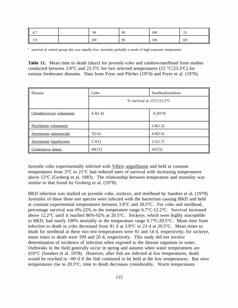
6.7 - 98 90 100 23

3.9 100 98 100 100

c survival of control group also was equally low; mortality probably a result of high exposure temperature

Table 11. Mean time to death (days) for juvenile coho and rainbow/steelhead from studiesconducted between 3.9°C and 23.3°C for two selected temperatures (15 °C/23.3°C) forvarious freshwater diseases. Data from Fryer and Pilcher (1974) and Fryer et al. (1976).

Disease Coho Steelhead/rainbow

% survival at 15°C/23.3°C

Chondrococcus columnaris 4.3(1.4) 4.2(0.9)

Flexibacter columnaris 5.8(1.2)

Aeromonas salmonicida 7(2.6) 4.9(2.6)

Aeromonas liquefaciens 2.3(1) 2.1(1.7)

Ceratomyxa shasta 40(12) 42(15)

Juvenile coho experimentally infected with Vibrio anguillarum and held at constanttemperatures from 3°C to 21°C had reduced rates of survival with increasing temperaturesabove 12°C (Groberg et al. 1983). The relationship between temperature and mortality wassimilar to that found by Groberg et al. (1978).

BKD infection was studied on juvenile coho, sockeye, and steelhead by Sanders et al. (1978). Juveniles of these three test species were infected with the bacterium causing BKD and heldat constant experimental temperatures between 3.9°C and 20.5°C. For coho and steelhead,percentage survival was 0%-22% in the temperature range 6.7°C-12.2°C. Survival increasedabove 12.2°C until it reached 86%-92% at 20.5°C. Sockeye, which were highly susceptibleto BKD, had nearly 100% mortality in the temperature range 6.7°C-20.5°C. Mean time frominfection to death in coho decreased from 81 d at 3.9°C to 23 d at 20.5°C. Mean times todeath for steelhead at these two test temperatures were 81 and 14 d, respectively; for sockeye,mean times to death were 109 and 20 d, respectively. This study did not involvedetermination of incidence of infection when exposed to the disease organism in water. Outbreaks in the field generally occur in spring and autumn when water temperatures are≤10°C (Sanders et al. 1978). However, after fish are infected at low temperatures, deathwould be reached in >80 d if the fish continued to be held at the low temperatures. But oncetemperatures rise to 20.5°C, time to death decreases considerably. Warm temperatures

115

(17.8°C to 20.5°C) might suppress incidence of infection, but once these salmonids areinfected at low temperatures, an increase in temperature simply hastens time to death.

IHN infection in rainbow trout responds in a similar manner to temperature as does BKDinfection (i.e., shorter survival time with higher temperatures after infection occurs). It isgenerally reported that IHN does not occur in the field above about 15°C (Hetrick et al.1979). However, if juvenile rainbow trout are infected at temperatures below 15°C and thentransferred to warmer temperatures, the course of the disease to death is faster. AlthoughAmend (1970, as cited by Hetrick et al. 1979) reported that IHN was prevented in juvenilesockeye when held at temperatures >18°C, Hetrick et al. (1979) found that fingerling rainbowtrout infection occurred at temperatures from 3°C to 18°C. At 12°C infected rainbowexperienced only 30% survival with a mean time to death of 10.7 d; at 15°C survival was48%; at 18°C survival from IHN was ≤54% (after subtracting mortalities of the control group)and mean time to death was reduced to 7.4 d. Because rainbow trout can become infected attemperatures up to 18°C, it appears that elevated temperatures are not a safety mechanismwhen confronted with IHN.

Proliferative kidney disease (PKD) was studied in juvenile rainbow trout in northern Ireland(Ferguson 1981). It was found that temperatures of 16°C stimulated full development of thedisease, but that declining temperatures were linked to inability of the disease to develop. PKD has been shown to affect chinook, steelhead, coho, brook trout, brown trout, andAtlantic salmon (Hedrick et al. 1984). It is caused by a protozoan that becomes activated attemperatures ≥15.6°C and causes enlargement of the kidney. PKD has been found in Idaho,California, and Vancouver Island.

116

GENETIC VARIATION IN RESPONSE TO THERMAL ENVIRONMENT

FAMILY-LEVEL VARIATION

Juvenile Survival and Preference

When comparing the temperature optima of major families of freshwater fishes found in theColumbia River drainage, a large degree of overlap is apparent. The family Salmonidae(salmon and trout) has temperature optima ranging from 5°C to 22°C. The other two majorcoldwater groups, the Coregonidae and Thymallidae, in North American freshwaters havevery similar ranges for temperature optima, 8°C-15°C and 4°C-18°C, respectively (Elliott1981). Chinook and the other Pacific salmon inhabit waters with a more restrictedtemperature range than exhibited by Salmonidae in general, have optima as high as 16°C. Avery meaningful, though infrequently used, indicator of thermal tolerance is the thermalpolygon (Elliott 1981). This index is computed as (°C)2 by determining the area bounded bythe upper and lower lethal limits on the acclimation-thermal exposure graph. Interestingly,despite the low tolerance demonstrated by coldwater stenotherms, they have relatively highresistance to thermal stress compared to warmwater eurytherms, which tend to behave in theinverse manner (Elliott 1981). Brett (1956) showed that the five species of North AmericanOncorhynchus have extremely low values (450-529°C2), even compared with brook trout(625°C2) and brown trout (583°C2). Goldfish, by contrast, have a value of 1220°C2. Mostcyprinids (e.g., shiners, dace, northern pikeminnow, except carp) have temperature optimaranging from 15°C-32°C) (Elliott 1981) and thermal tolerance indices ranging fromapproximately 750 to 900°C2 (Brett 1956). Centrarchids (e.g., bass) have temperature optimamuch like the cyprinids. For example, smallmouth bass prefer temperatures of 21.4°C andhave an upper lethal limit of 35°C (Scott and Crossman 1985). The optimum growthtemperature for juveniles is 26°C (Horning and Pearson 1973).

Temperature preferences are a very good indicator of physiological temperature optima (Brett1971). Temperature preferences for various representatives of Salmonidae, Cyprinidae, andCentrarchidae, and other groups were compiled by Coutant (1977). A brief summary ofultimate preferenda (means of all the references provided, sorted by age, and considering onlysummer preference when given) is provided in Table 12. This table is not comprehensive forall currently available literature but does provide a rapid view of the major differences amongfish families using a readily accessible review. Not all species listed of the Cyprinidae, andCentrarchidae have been introduced into the Pacific Northwest, but these species adequatelyrepresent other members of the family for purposes here.

117

Table 12. Ultimate temperature preferenda for various representative Salmonidae, Cyprinidae,and Centrarchidae. Values are means computed from tabulated values in Coutant (1977),considering only summer preference when seasonal data are provided. In cases wheremultiple estimates were made on similar size fish by a single investigator, all those valueswere averaged and attributed to only one reference.

Species Common Name References Ultimatepreferendum

(°C)

Salmonidae

Oncorhynchustshawytscha

chinook salmon Brett (1952)Spigarelli (1975)

11.7 (young)17.3 (adult)

Oncorhynchus nerka sockeye salmon Horak and Tanner (1964) 11.7

Salmo gairdneri rainbow trout McCauley and Pond (1971)Horak and Tanner (1964), Garside andTait (1958), Spigarelli (1975), Cherryet al. (1975)

18.5(fingerling)

16.9 (adult)

Cyprinidae

Notropis atherinoides emerald shiner Barans and Tubb (1973)

Barans and Tubb (1973)

22.5 (YOY)

23 (adult)

Notemigonuscrysoleucas

golden shiner Reutter and Herdendorf (1974) 22.3 (adult)

Pimephales promelas fathead minnow Jones and Irwin (1965)Cherry et al. (1975)

23.4 (<74 mm)29 (adult)

Pimephales notatus bluntnoseminnow

Cherry et al. (1975) 29 (adult)

Centrarchidae

Micropterus salmoides largemouth bass Dendy (1948), Clugston (1973), Neill(1971), Coutant (1975), Ferguson(1958), Reynolds et al. (1976),Reynolds and Casterlin (1976),

28.8 (all sizes)

Micropterus dolomieui smallmouthbass

Barans and Tubb (1973)Barans and Tubb (1973)

31 (YOY)29 (adult)

118

Lepomis gibbosus pumpkinseed Neill (1971), Reutter and Herdendorf(1974), Reynolds, unpubl.

28.6 (small toadult)

Lepomis macrochirus bluegill Neill (1971), Ferguson (1958),Beittinger (1974), Reynolds andCasterlin (1976), Reynolds et al.(1976)

Cherry et al. (1975)

31.7 (53-155mm+young)

32 (adult)

The UUILT is not always identified precisely in the literature but a small increase in upperincipient lethal limit with substantial increase in acclimation temperature is a good indicationthat the ultimate incipient level is reached. Given the data compilation for Salmonidae in thisreport (Tables 3 and 4) and the compilation by Coutant (1972), one can infer a range ofUUILT for the families Salmonidae, Cyprinidae, and Centrarchidae, to be 23°C-25.6°C(Tables 3 and 4), 29°C-33°C (Table 13), and 33°C-37°C (Table 14), respectively. This rangein UUILT values mentioned for Salmonidae accounts for the response of the species chinook,coho, sockeye, chum, and pink salmon, steelhead, Atlantic salmon, brown, brook, and laketrout. There appears to be very little variation in UUILT among species in family groups,except for a higher lethal limit for redband trout and a lower one for bull trout.

Table 13. UILT values for various Cyprinidae--dace, minnows, chubs, shiners, (except carp)from the literature as representative for the family. Values taken from Coutant (1972).

Species Common Name References AcclimationTemperature

(°C)

ExposureTemperature

(°C)

Rhinichthysatratulus

blacknose dace Hart (1947) 2025

29.329.3

Notropisatherinoides

emerald shiner Hart (1947) 2025

30.730.7

Notropis cornutus common shiner Hart (1952) 2025

31.031.0

Semotilusatromaculatus

creek chub Hart (1952) 2025

30.331.5

Notemigonuscrysoleucas

golden shiner Hart (1952) 202530

32.033.534.5

Pimephalespromelas

fathead minnow Hart (1952) 2030

31.733.2

119

Pimephales notatus bluntnose minnow Hart (1952) 2025

31.733.3

Table 14. UILT values for various Centrarchidae from the literature as representative for thefamily. Values taken from Coutant (1972) and Brungs and Jones (1977).

Species Common Name References AcclimationTemperature

(°C)

ExposureTemperature

(°C)

Micropterussalmoides

largemouth bass Hart (1952) 2030

3233.7

Lepomis megalotis longear sunfish Neill, Strawn, andDunn (1966)

30 36.8

Lepomismacrochirus

bluegill Hart (1952) 2030

3233.8

* acclimation temperature not given

SPECIES-LEVEL VARIATION

Egg/Alevin Survival and Development

Murray and McPhail (1988) provided a very detailed investigation of effects of incubationtemperature on five species of Pacific salmon (chinook, coho, sockeye, chum, and pinksalmon). They measured effects of five incubation temperatures (2, 5, 8, 11, and 14°C) onfertilization-to-hatching and hatching-to-emergence stages. These species appear to beadapted to different spawning times and temperatures (Murray and McPhail 1988);consequently, by selection of spawning time the incubation temperature regime can bematched to the species' needs so that high survival is likely. High survival during incubationinvolves avoidance of high intragravel temperatures immediately after spawning (in autumnspawning species) and avoidance of extremely low temperatures during winter. Temperatureslow enough to be lethal may occur in high altitude spawning zones (e.g., spring chinook orsteelhead reaches) or in low gradient reaches dominated by glacial- or snowmelt. Lethal lowtemperatures are also more likely where riparian cover has been removed in regionsdominated by continental air masses and clear skies. High survival at emergence is afunction of avoiding instantaneous temperature extremes (high and low) and accumulating thenecessary thermal units so that emergence is timed to correspond to moderate dischargeregimes. Emergence timing also influences the potential for growth to a size class capable of

120

emigrating. For example, early emergence by coho allows them to grow for a longer periodbefore their first winter than other salmon that do not emerge early. Size at emigration isdirectly related to smolt-to-adult survival rate. If multiple years of freshwater rearing arenecessary because of slow growth rate, percentage mortality increases with overwinter rearingin natal habitats but may be somewhat compensated by higher survival of resulting largersmolts.

Murray and McPhail (1988) found important variation among salmon species in their earlydevelopment. When incubated at the high temperature (14°C), chum, pink, and chinooksurvived better than coho and sockeye. All five species suffered reduction in alevin and frysize when incubated at 14°C. When incubated at the lowest temperature (2°C), no pink orchum embryos survived. Chinook survival rate was lower than that of coho or sockeye. Thelargest fry of coho, chinook, chum, pink, and sockeye were produced by constant incubationtemperatures of 2, 5, 5, 8, and 8°C, respectively. Coho hatched and emerged sooner at alltemperatures than the other species. The time from fertilization to 50% emergence in pinksalmon at 8, 11, and 14°C was greater than the other species. But when incubated at 2°C and5°C, chinook required the most time to reach 50% emergence. At 8°C embryos of all fivespecies had their highest survival rates. Variation among species in embryo survival rate wasalso lowest at 8°C but increased at the extremes of incubation temperatures used (i.e., at 2and 14°C). Beacham and Murray (1990) found significant differences among these same fivespecies of Pacific salmon in response of alevin length, weight, yolk weight, and tissue weightto incubation temperature. They determined that 60% of total variance was accounted for byspecies. These authors also found variation among species in development rate, embryo andalevin survival, and fry size at various incubation temperatures. For example, coho is adaptedto late autumn to early winter spawning and low water temperatures. It also has the fastestdevelopment rate to hatching and emergence, highest embryo survival rate and largest alevinand fry at incubation temperatures <4°C (Beacham and Murray 1990). Its greater rate ofdevelopment at low temperatures compensates for late spawning.

Inter-specific hatching success was studied in various coldwater species by Humpesch (1985).He found highest hatching success (>90%) for all species incubated within their optimumtemperature range. Hatching success was >90% for each species at their optimumtemperatures. Optimum temperature varied from 5°C for brown trout, Arctic char, and brooktrout, 8°C for Danube salmon, to 7°C-11°C for rainbow and grayling. Within temperatureranges given in Table 15 he measured high hatching success (>80%), which dropped off attemperatures higher and lower than the ranges specified. This relationship was described by abell-shaped curve for each species. Upper hatching limits (i.e., the upper temperature atwhich hatching success reached 0%) varied from 12.5 to 18.5°C. Lower hatching limits (i.e.,the lower temperature at which hatching success reaches 0%) varied from <1 to 3°C. Time tohatching at 10°C incubation temperature varied among species. Of the five species in Table15, rainbow hatched most rapidly at 10°C while brook trout, Arctic char, and grayling allrequired up to about 53 d to reach 50% hatching. There is variation among researchers indays to 50% hatching success within a species that reflects intra-specific variation but alsoresearch technique to an unknown extent. Given these sources of variation, the actual

121

variation is actually small. Within the well-studied species, Salmo gairdneri, Humpesch'sreview indicated a range in days to 50% hatch at 10°C of 31 to 36 d. At 5°C incubationHumpesch (1985) measured 71-75 d to 50% hatch. Including the data from five other authorsexpands this range to 52-91 d. Given the four stocks of brown trout studied by Humpesch,38-42 d were required to 50% hatching at 10°C, indicating little intra-specific variation. Adding the data from four other authors expands this range to 38-52 d.

Table 15. Interspecific variation in hatching temperatures and days to 50% hatching inseveral coldwater fish species. Data from Humpesch (1985).

Species Temperaturerange for>80%hatchingsuccess (°C)

Upperhatching limit(°C)

Lowerhatching limit(°C)

Time to50%hatchingat 10°C(d)

Salvelinus fontinalis 1.5-9 15 <1 37-53

Salvelinus alpinus 1.5-5 12.5 <1 46-53

Salmo gairdneri 10-12 18.5 3 32-34

Salmo trutta 1-10 15 <1 38-42

Thymallusthymallus

7-12 18.5 3 48-54


Temperature preferences in salmonids are thought to reflect physiological optima (Brett1971). In addition, final preference tends to be a good index to optimum growth temperature(Jobling 1981)

Peterson et al. (1979) studied the temperature preferences of several species of salmonidsincluding rainbow trout (Oncorhynchus mykiss), anadromous and landlocked Atlantic salmon(Salmo salar), brook trout (Salvelinus fontinalis), lake trout (Salvelinus namaycush), andArctic char (Salvelinus alpinus) (Table 16). Because fry were allowed 1 h and fingerlings 2 hfor adjustment to test conditions, followed by a 64-min determination of frequencydistribution at 2-min intervals in a horizontal temperature gradient tank, this test should beconsidered to be an acute preference test. Acronyms for these species are Om, Ss, Sf, Sn,and Sa, respectively. Hybrids of these species were also tested. Fry of the species testedpreferred different temperature ranges. The Oncorhynchus/Salmo group selected temperaturesof 13.6°C to 14.3°C. Within the Salvelinus genus preferred temperatures of fry were 8.7°C to

122

9.9°C. The Salvelinus hybrids preferred temperatures ranging from 9.2 to 10.5°C. There wasa very small difference between anadromous and landlocked salmon fry.

Oncorhynchus mykiss and Salvelinus namaycush fingerlings preferred similar temperatures asfry. However, fingerlings of Salvelinus fontinalis and the (Sf x Sn ) and (Sn x Sf )hybrids preferred higher temperatures than the corresponding fry. The hybrids of thefingerlings were also intermediate between the pure strains. Genetic differences weredetected between genera and between hybrids and the pure parent strains. However, therewere no differences within a species in the case of anadromous and landlocked forms ofSalmo salar and very little difference in preference among fry of the three Salvelinus speciestested.

Table 16. Results of thermal preference tests of Peterson et al. (1979) for fry and fingerlingsof several species and hybrids of salmonids. Oncorhynchus mykiss, Salmo salar, Salvelinusfontinalis, Salvelinus namaycush, and Salvelinus alpinus are symbolized as Om, Ss, Sf, Sn,and Sa, respectively..

Species or hybrid fry* fingerlings**

Om 14.3 14.7

Ss (anadromous) 13.8

Ss (landlocked) 13.6

Sf 8.7 17.5

Sa 9.2

Sn 9.9 10.8

Sa x Sf 9.2

Sf x Sa 10.5

Sf x Sn 9.4 14.7

Sn x Sf 10.1 14.4

* acclimation temperature of fry was 12.7°C** acclimation temperature of fingerlings was 12.1°C

Goddard and Tait (1976) measured the preferred temperatures of yearling F3 to F5 hybridsfrom an original F1 created from a Sn x Sf cross. Progeny of the F1 were subjected toselection for early maturity in succeeding generations. Between the F3 and F5 generations, final preferred temperatures of hybrids acclimated to 12°C decreased from 16.3°C (F3) to14.8°C (F5). Goddard and Tait noted a reduction in temperature preference with eachsuccessive generation from one typical of brook trout toward that of lake trout (near 11.7°C).

123

The F5 hybrid temperature preference with 12°C acclimation is similar to that reported byPeterson et al. (1979) for their fingerling F1 hybrid from a Sn x Sf cross acclimated to12.1°C. The mean length of the F5 hybrids of Goddard and Tait was 137.2 mm; that of thefingerling F1 hybrid of Peterson et al. was 61.7 mm. It is possible that the size difference ofthe F1 hybrids tested was partially responsible for the differences in preference observed. Even though Goddard and Tait were able to breed hybrid strains with varying degrees oftemperature preference, the preference of the hybrid was confined by the temperature rangesof the parent species. Peterson et al. (1979) also found that the F1 hybrids preferredtemperatures intermediate between that of the parent species.

In a study evaluating the relationship between acute temperature preference and acclimationtemperature within three families (Cyprinidae, Ictaluridae, and Centrarchidae), Mathur et al.(1981) noted that less than 2% of total variance in temperature preference among specieswithin a family was accounted for by the species effect. Most of the variation among specieswithin a family (64%-81%) was due to acclimation temperature and less than 2% wasattributable to species. Even though the species effect was statistically significant in the caseof the Cyprinidae and Ictaluridae, Mathur et al. (1981) concluded that this effect wasbiologically trivial. They considered that a biologically significant effect would be more thanbarely discernible with a large sample size, but should be related to magnitude of thedifference. Hart (1952) also considered that the effect of acclimation temperature maycompletely obscure differences at the species or racial level. In addition, he noted thatdifferences in age, size, water chemistry, and season must also be controlled when comparingpopulations because these factors also lead to variation in response. Variability in acutepreference is great enough within a population that geographic variation would be difficult todemonstrate (Mathur et al. 1981).

A portion of the variation in temperature preferences or UUILT or CTM values reported inthe literature is attributable to variation in methodology and unique test conditions applied bythe experimenter (Mathur et al. 1981). As typical with all experimental work, sources ofinterspecific variation among literature on temperature effects include genetic differencesamong the test organisms; differences among species linked to acclimation, nutritional orhealth status, life stage, etc. of the test groups; uncontrolled environmental variation from onetest period to another or among test groups or sites; and measurement error. One means ofreducing variation associated with species effects is to evaluate a single published study on avariety of species in which a common laboratory protocol was applied to each species.

Cherry et al. (1977) studied preferred and lethal temperatures for several species of salmonids,cyprinids, and centrarchids. Final temperature preferences for representatives of thesefamilies were <19, >24, and >29°C, respectively. The 7-d UUILT for these groups,respectively, was 23-25, 26-36, and 35°C-36°C. Within the salmonids, rainbow trout, browntrout, and brook trout avoided temperatures outside the bounds 15-26, 17-25, and 18°C-26°C,respectively. The 7-d UUILT values for these three salmonids, respectively, were 25, 23, and24°C.

124

Brett (1952) measured UUILT on several salmon species (Oncorhynchus tshawytscha, O.kisutch, O. gorbuscha, O. keta, and O. nerka). Brett's work is the most complete analysis ofthermal effects on fish physiology available in the literature. It provides a useful comparisonof these five species. He found that among species of Pacific salmon the UUILT valuesvaried only from 23.8°C-25.1°C. Brett's detailed studies, reported in several publications, isrivaled only by Elliott's work on brown trout (Elliott 1975a, 1975b, Elliott 1994).

Lee and Rinne (1980) studied the critical thermal maxima (CTM) to loss of equilibrium (LE-temperature of Becker and Genoway 1979) of five species of trout (15-20 cm total length anddescribed as adults) collected in the southwestern U.S. Rainbow trout (formerly Salmogairdneri, currently O. mykiss), brown trout (Salmo trutta), and brook trout (Salvelinusfontinalis) were introduced species; Gila trout (Salmo gilae) and Arizona trout (Salmo apache)are native. These five species had CTM values for 20°C acclimation and 1.2°C/h temperatureincrease of 29.4, 29.9, 29.8, 29.6, and 29.4°C, respectively. The LE-temperature for cohoacclimated at 15°C and subjected to an equivalent temperature rise to that used by Lee andRinne (1°C/h) was 27.7°C (Becker and Genoway 1979). A higher acclimation temperaturefor coho would likely have made the coho CTM value even more similar to those of the troutspecies. The similarity in CTM values for these six salmonids from different geneticbackgrounds and environments makes it seem unlikely to expect broad levels of adaptationwithin a species that are not seen among species.

Juvenile Growth

Sadler et al. (1986) studied variation in fingerling growth rate among species (brook trout,lake trout and rainbow trout) at two constant temperatures. At 10°C the rank of specificgrowth rate from low to high was brook trout, lake trout, and rainbow trout. At 16°C rankingfrom low to high was lake trout, rainbow trout, and brook trout. Only lake trout had nodifference in specific growth rate at these two temperatures. A lake trout x brook trouthybrid tested had a growth rate that was intermediate between that of the parents. Brooktrout, rainbow trout, and splake (Sn x Sf ) were significantly higher at 16°C than at 10°C. The preferred temperatures of lake trout and brook trout, respectively were 11.7°C (McCauleyand Tait 1970) and 17°C (McCauley and Casselman 1981) (both as cited by Sadler et al.1986). Rainbow trout fingerlings, provided a temperature gradient from 12 to 28°C invertical and horizontal gradient laboratory tanks, preferred a mean of 18.4°C in both tanks(McCauley and Pond 1971). Temperature preference appeared to be related to the optimumrange for growth. Also, in lake trout their food conversion efficiency declined significantlywhen rearing at the higher temperature.

STOCK-LEVEL VARIATION


Murray and Beacham (1986) studied the survival and rate of development of pink salmon(Oncorhynchus gorbuscha) eggs from five different British Columbia stocks under various

125

temperature regimes. For their pink salmon studies in which stock differences wereexamined, the incubation temperature regime used was a transfer from initial hightemperatures (either 8°C or 12°C) to 1°C at various stages of embryo development. Eggs ofall stocks were fertilized at 8°C and then held at either 8°C or 12°C for 36 d. The eggs heldat 8°C reached stage 26 (onset of operculum growth) and those incubated at 12°C reacheddevelopmental stage 29 (near hatching) in this 36-d period. Embryos were then transferred toa 1°C bath. Egg survival was more variable among stocks than among families within stocksfrom the point of transfer to 1°C to termination (day 133 to 150 of development). For threestocks, egg survival rates were similar when made at stages 26 or 29. The other two stockseach had significant differences in survival between transfers at these two stages. Under anygiven temperature regime there was no stock difference in time to 50% hatching. Survival tohatching was uniformly high (>88%) among all five stocks surveyed in transfers from 8°C or12°C to 1°C. Alevin survival was low (38%-60%) for all stocks studied after hatching,except for the most northerly stock (Keogh River), when eggs incubated at 12°C weretransferred to 1°C at hatching. The authors suggest that more northerly stocks may be betteradapted to greater temperature reduction later in embryo development.

Survival can be partially a function of egg size and size of alevin at hatching or size ofemergent fry (a function of egg size and incubation temperature). A portion of this survivalis expressed in development to emergence (e.g., ability of fry to emerge from a gravelbed),but egg size and temperature conditions resulting in larger emergent fry also can lead togreater early ocean survival. Temperature regime is governed by a combination of theinherent climatic and hydrologic regime for the stock and land management influences on thevegetative cover in the watershed (especially the riparian zone). Egg size is determinedfirstly by species effects and secondarily by stock effect, size and age of female, season, andnutritional status. Beacham et al. (1988) measured morphometric differences in pink salmonamong stocks within broodlines (i.e., even- and odd-year) and also between broodlines. Theyfound that morphometric characters (adult size, head size, caudal peduncle thickness, fin size)varied more among stocks within broodlines than between broodlines. However, on the basisof allelic frequencies, variation between broodlines was greater than variation among stockswithin a broodline. The morphometric variation among stocks or differences betweenbroodlines could indicate adaptation to the natal river conditions (Beacham 1985, as cited byBeacham et al. 1988). Fish spawning in larger rivers within the geographic range surveyed(British Columbia) were larger in all morphometric characters measured than in smallerrivers. Odd-year stocks typically have larger eggs than even-year stocks for equivalent bodylengths, even when both stocks originate from the same river (Bilton and Smith 1973). Thisegg size advantage, such as observed in the Babine odd-year pink run, is translated to largerfry and also larger adults (Bilton and Smith 1973). Also, within a stock, the mean length ofmales and females and the weight of eggs increased as the spawning season progressed(Beacham et al. 1988).

There are great variations in migration distances among stocks of both chinook and sockeyein British Columbia as well as the Columbia River. Sockeye migration distances vary fromthe coastal area to 700 km upriver in the Fraser River and chinook migrate distances ranging

126

from the coastal area to >1000 km upriver. These different spawning environments result inthe interior-spawning stocks (ISS) being adapted to cold winter climates and the coastal-spawning stocks (CSS) adapting to mild winter conditions. Interior stocks of both species hadsmaller eggs than the coastal stocks and had higher embryo survival rates at lower incubationtemperatures (Beacham and Murray 1989). The smaller egg size (and lower fecundity) of ISSstocks may be caused by the need to convert available energy to swimming greater distancesrather than egg production. In sockeye studied, among stock variation in egg diameteraccounted for 82% of total egg diameter variation, while differences among femalesaccounted for 10% of the variation. In chinook, among stock variation accounted for 37% oftotal egg diameter variation, whereas differences among females accounted for 42% of eggdiameter variation. No significant differences in egg size were detected between red-fleshedand white-fleshed chinook.

Beacham and Murray (1989) studied survival and development of two sockeye stocks (1 ISSand 1 CSS stock) and three chinook stocks (1 ISS and 2 CSS). When the eggs of ISS andCSS sockeye and chinook stocks were incubated under constant temperatures of 2, 4, 8, 12,and 15°C, the ISS developmental rates to hatching and emergence were faster than those ofCSS. This implies that ISS stocks were more efficient in metabolizing yolk at lowtemperatures than were CSS stocks (Beacham and Murray 1989). Survival rates of ISS tohatching and emergence were higher than for CSS at low incubation temperatures, whichcould indicate their adaptation to colder thermal conditions. At 2°C the survival rates of theCSS and ISS sockeye stocks were 33% and 91%, respectively, from fertilization to hatching. Subsequent survival from hatching to emergence was high for each stock (>95%). Nochinook embryos of either stock group (CSS or ISS) survived at 2°C incubation to hatching. However, the CSS and ISS stocks compared in the study by Beacham and Murray (1989)were from southern British Columbia. A northern British Columbia chinook ISS stock(Babine River) studied by Murray and McPhail (1988) had 14% survival from fertilization toemergence at 2°C. Beacham and Murray (1989) concluded, on the basis of their data and thatof Alderdice and Velsen (1978), that an incubation temperature of 3°C results in a 50%chinook embryo mortality. In sockeye 50% mortality was produced at incubationtemperatures of 1°C to 3°C, depending upon stock. Alevin survival rates were differentamong sockeye stocks and among chinook stocks only at 15°C. In sockeye, survival for theCSS stock was higher than for the ISS stock at 15°C; in chinook one CSS stock hadrelatively low survival at 15°C (56%) compared to the ISS stock (90%) and the other CSSstock (87%). Beacham and Murray (1989) attributed the better performance of CSS sockeyeat 15°C to their greater degree of adaptation to milder climates. However, by this reasoningit is difficult to explain the low survival of the CSS chinook stock.

Sockeye alevins of all stocks were longest when incubated at either 4°C or 8°C and shortestat 15°C (Beacham and Murray 1989). Chinook alevins were longest at 4°C. Both sockeyeand chinook alevins were heaviest at 8°C and had the greatest amount of yolk at 15°C. Sockeye fry were longest at 4°C whereas chinook fry were longest at 8°C. Both sockeye andchinook fry were lightest at 15°C incubation. Fry of sockeye and chinook both had thegreatest amount of yolk remaining at emergence when incubated at 15°C. However, in

127

converting yolk to tissue, the ISS sockeye stock had better growth (conversion of yolk totissue) at 2°C relative to that at 8°C than the CSS sockeye stock. The authors hypothesizedthat this reflects a greater adaptation of the ISS stock to low incubation temperature. Stockdifferences were observed in alevin and fry length, total weight, yolk weight, and tissueweight in both sockeye and chinook. However, these differences were related to initial eggsize of the stock. For both sockeye and chinook, adult females of the CSS and ISS stockswere similar in length, but the ISS stocks of each species had significantly smaller eggs thanthe CSS stocks. In sockeye, stocks accounted for 82% of total variance in egg diameter andfemales within stocks accounted for only 9% of egg diameter variance. In chinookcomparable assignment of variance was 37% and 42%, respectively.

Two forms of chinook were also compared by Beacham and Murray (1989), red-fleshed andwhite-fleshed forms from the Quesnel River. Red-fleshed chinook incubated at 15°C hadsignificantly higher embryo survival rates than the white-fleshed variety, although thecomparative differences were small (98% vs. 92%). Carotenoids in the eggs of red-fleshedchinook may improve oxygen uptake by eggs at higher temperatures, improve percentagesurvival to hatching, and may also aid in egg respiration when held in the body cavity ofoverripe females waiting to spawn (Craik 1985). The environment of loose eggs in theabdominal cavity of overripe females holding in warm water conditions is one of low oxygen(Flett et al. 1996, Craik 1985, de Gaudemar and Beall 1998).

With the species odd-year pink, chum, and sockeye salmon, the variation in alevin hatchingand fry emergence times is related to time of spawning. Those populations with earlyspawning time also have late alevin hatching and late fry emergence. Hatching time of even-year pink alevins was later than for odd-year alevins at all test temperatures (Beacham andMurray 1990).

Populations of kokanee from Hill and Mackenzie Creeks flowing into the northeastern side ofUpper Arrow Lake in southeastern British Columbia were found to have similar embryo andalevin survival rates for all temperatures tested between 2°C and 10°C (Murray et al. 1989). Embryo survival was >80% at temperatures from 4°C to 10°C, but was only 60% at 2°C forthe two populations. Embryo mortality at 2°C occurred in epiboly. Alevin survival washomogeneously >90% at all temperatures from 2°C-10°C. Days to 50% hatching and 50%emergence for these two populations were also similar and varied inversely with meanincubation temperature.

One of the most extensive studies ever conducted on the influence of parental stock andtemperature on egg/alevin survival and development was that of Murray et al. (1990) on 13stocks of coho in British Columbia. These stocks spanned a wide geographic region thatincorporated effects of northern vs. southern stocks (i.e., latitudinal effects) and island vs.mainland (i.e., moderate coastal climate vs. cold winter mainland climate). Coho gameteswere collected from 13 different stocks. Eggs from single females were fertilized with spermfrom single males, producing 5 full-sib families per stock. Eggs were incubated intemperature baths of 2, 5, 8, 11, and 14°C. There were significant differences among stocks

128

in egg diameter and weight that were related to female postorbital-hypural length. Stockeffect accounted for 74% of total variance in egg weight and female length accounted for23% of the total variance in egg weight.

In the stage from fertilization to hatching, survival of embryos for most of the 13 coho stockswas highest at 4°C or 5°C and were >85% at 2, 4, 5, and 8°C (Murray et al. 1990). Of thethree island stocks, two of them (i.e., Pallant Creek and Roberstson Creek) had low embryosurvival rates (approximately 65%) at 1.5°C. Complete mortality occurred at 14°C and 15°Cin all stocks (except for two families of the Coho Creek stock in 1979). For alevins, survivalrates in the 1976-1979 studies were not significantly different among stocks for a giventemperature, except at 2°C. At this temperature stocks from Coho Creek and Salmon River(two of the ten mainland stocks) had significantly higher survival rates than the other stocks. However, in 1986 alevin survival rates to emergence were significantly different amongstocks within temperatures 1.5, 2, 8, and 12°C, but not 4°C. Over the entire period fromfertilization to 50% emergence, there were significant differences in development time amongstocks and among temperatures. However, stocks that hatched early at one temperature werenot consistently early at all other temperatures (i.e., there was an interaction effect of stocksand temperature in the ANOVA design).

For the 13 coho stocks surveyed in 1976-1979 no significant difference existed among stocksin alevin standard length or total wet weight, but differences among stocks were found amongincubation temperatures (Murray et al. 1990). Alevin length and weight were typicallyhighest at low incubation temperatures and decreased with increasing temperature. Alevinlength was shortest at 12°C. In the 1976-1979 surveys there were no significant differencesamong stocks in fry standard length or total weight, but incubation temperature produced asignificant effect. The longest and heaviest fry developed at 5°C. In the 1986 survey thelongest fry and greatest weight at emergence developed at 4°C and 8°C and the shortest andlightest at 1.5°C.

Regional differences among stocks were apparent in the studies on coho by Murray et al.(1990). Northern stocks were more efficient at converting yolk to either alevin or fry tissueat 1.5°C than were southern stocks. At this same temperature mainland stocks were moreefficient than island stocks. The converse was true at a warmer temperature (8°C) in thesetwo regional comparisons. This implies that there are significant genetic adaptations relativeto temperature that improve the efficiency, and presumably fitness, of stocks to cope withtheir environments. However, if fry total weight at emergence is also a good index to fitnessat a given temperature, there was no stock difference observed in fry total weight in the 1976-1979 surveys. Another unifying principle in this stock comparison is that across all stockssurveyed, 14°C was the upper threshold for normal development and 0.6°C-1.3°C was thelower threshold. However, within these bounds there were significant effects of incubationtemperature that can vary the survival or developmental rates to hatching and emergence andthe yolk conversion efficiencies.

129

Beacham (1988) studied the genetic differences between two stocks of pink and two stocks ofchum salmon from Alaska. Chum from the Kshwan and Bella Coola Rivers and pink salmonfrom the Quinsam and Harrison Rivers provided the comparisons . A total of 25 families,produced from adults sampled from each river, were the basis for calculating mean survivalrates. Survival rates of chum eggs were tested at constant temperatures of 3.1, 8.0, and15.1°C; pink eggs were tested at 4.1, 8.0, and 15.9°C. For chum, only at the low temperaturewere embryo survival rates different between stocks (70.1 and 93.9%, respectively). In pinksalmon, alevin survival rates were significantly different at the high temperature (45.7 and87.8%, respectively) and embryo survival rates were significantly different at the lowtemperature (38.4 and 47.0%, respectively). In both species there was a significant differencebetween stocks in the hatching and button-up times at the lowest incubation temperature.

Cutthroat and rainbow trout introduced into Emerald Lake, Colorado in 1888-1890 (Lentsch1985, Van Velson 1985) (as cited by Behnke 1992) have had 20-25 generations in the lakeand have formed a hybridized population. The outlet stream accumulates twice the number oftemperature units as the inlet stream during the incubation period of these species (i.e.,spawning to emergence). At a 12°C incubation temperature, both inlet and outlet spawnershatched at 330 temperature units. This study implies that there has been no selection fordevelopment rate in the two stocks originating from the original planting despite theirsubstantially different incubation environments. Unfortunately, in this study developmentrates were not tested at the low temperatures experienced in the inlet stream (minimum of2°C in June, maximum of 6°C during summer) to assess whether the low temperature inletpopulation performs better at 2°C than the outlet population.

Humpesch (1985) studied inter- and intra-specific variation in hatching success and embryonicdevelopment of five salmonid species (brook trout, Salvelinus fontinalis; Arctic char,Salvelinus alpinus; rainbow trout, Salmo gairdneri; brown trout, Salmo trutta; Danube salmon,Hucho hucho; and grayling, Thymallus thymallus). Brown trout were collected from a lakeoutlet stream, a summer-cool lowland stream, a summer-cool upland stream, and an alpinelake. Grayling stocks were collected from two summer-cool rivers in a mountainous area. Humpesch considered these various habitats for these species to be thermally distinct. Theregressions of hatching success on incubation temperature provided regression coefficients aand b. These were not significantly different among stocks within the species studied.

Variation in egg and embryo response to elevated temperatures was studied in twogeographically distant stocks of largemouth bass, Micropterus salmoides salmoides (a northernstock from Minnesota and Wisconsin and a southern stock from Tennessee) (McCormick andWegner 1981). The median temperature tolerance limits (TL50) for 0-3-d-old hatched larvaeaveraged 32.1°C and 32.6°C for the northern and southern stocks, respectively, for larvaeacclimated to 20, 24, 27, and 30°C. There was very little difference in TL50 values at allthese acclimation temperatures, allowing them to be averaged. When acclimated to 22°C,newly hatched larvae had 24-h TL50 values of 31.0°C and 30.6°C for the northern andsouthern stocks, respectively. Differences between stocks in all but one of the temperaturechallenges were ≤0.5°C. Despite the great difference in geographic latitude between the

130

stocks compared, they were homogeneous in response to thermal stress within this subspecies.


McCauley (1958) indicated that tests of the upper lethal temperatures for two races (notrecognized as separate subspecies) of Salvelinus fontinalis failed to reveal any difference inresponse. The geometric mean resistance at 1000 min exposure occurred at 26°C with 20°Cacclimation. However, McCauley reported a difference in response between two subspeciesof Salvelinus alpinus (i.e., S. a. willughbii and S. a. alpinus). However, the geometric meanresistance at 1000 min exposure occurred at approximately 24.7°C with S. a. willughbii and at24.4°C with S. a. alpinus. Even though McCauley reported a highly significant differencebetween the subspecies, the actual difference in thermal tolerance was negligible in amanagement context.

Elliott (1981) pointed out how genetic differences that are often assumed between differentpopulations of a species are frequently found not to be significant. He reported an examplein which brown and rainbow trout living in a stream with daily maximum temperatures of28.8°C did not have greater thermal tolerances when compared with trout from two hatcheries(Kaya 1978). Brett (1956) reported that what is taken as geographical variation is oftennothing more that variability owing to experimental method and acclimation temperatures. Konecki et al. (1995a) measured CTM values at streamside of three coho populations inWashington coastal streams that varied in thermal regime and found apparent differences. However, after providing approximately a 3-month acclimation at a constant temperature, theCTM values were not significantly different. Mathur and Silver (1980) showed that thereported statistically different preference temperatures measured by Hall et al. (1978) for threewhite perch populations (from North Carolina, Maryland, and New Jersey) were actually non-significant when the correct number of degrees of freedom were applied to the statisticalanalysis. Repeated recording of the temperature selected by an individual fish in a gradientproduces a set of highly correlated observations, inflating the degrees of freedom. Also, ifmany fish are tested in an apparatus at the same time, preferences are affected by behavioralinteractions (Mathur and Silver 1980).

Beacham and Withler (1991) studied the survival of ocean-type and stream-type juvenilechinook to high water temperatures. Twenty separate full-sib families of the ocean-type(hatchery) and 32 full-sib families of the stream-type chinook (wild) were produced fromgamete collections and matings of 1 male with each of 2 females. Fifteen juveniles fromeach of the families were tested separately at high temperature rearing conditions. Thestream-type population, rearing at 21.5°C, had a total mortality of 79% after 16 d. Theocean-type population, rearing at 22°C, had a total mortality of 74% after 18 d. Thesepopulations responded very similarly to high temperature (approximately 22°C) in about 18 dof exposure but the cumulative mortality curves were very different. The stream-typepopulation had approximately 70% mortality after 8 d, whereas the ocean-type populationsuffered only 3% mortality in the same time period. These different patterns of mortality arelikely a result of adaptive differences in the populations (Beacham and Withler 1991). The

131

authors speculated that ocean-type chinook are better adapted to warmer water conditionsbecause they spend a greater portion of their life cycle in coastal waters.

Genetic selection for disease resistance has been shown to vary among populations or strainsof salmonids. For example, susceptibility to furunculosis and vibriosis infection varies amongpopulations (see citations in Beacham and Evelyn 1992). Survival and mean time to death offish having these diseases depends upon temperature exposure. A population highly resistantto one disease may not be equally resistant to another disease. Additive genetic variationallows selection for some degree of resistance to diseases.

The UILTs of four widely dispersed rainbow trout populations from four Great Lakeswatersheds were determined on fry acclimated to 15°C at a rate of 1°C/d (Bidgood and Berst1969). Fry were tested at 25, 26, 27, 28, 29, and 30°C. Fry were able to tolerate 25°C for4 d but the UILT was between 25 and 26°C. This species had been introduced to LakeSuperior in 1895 but no differences in UILT were determined among these populations. Either the populations were all using similar environments or a 100-year period is notsufficient for differences in UILT to appear.

CTM was studied in two strains of Lahontan cutthroat trout (Salvelinus clarki henshawi) byVigg and Koch (1980). These two strains were the Summit Lake strain, which may bedescended from the Pyramid Lake strain, and the Marble Bluff strain, taken from the TruckeeRiver mouth. CTM was determined by raising water temperature by 1°C/d, starting from anacclimation temperature of 16°C. After 20°C was reached, temperatures were raised by 1°Cevery 4 d. In Truckee River water, the Summit Lake and Marble Bluff strains reached the D-temperature (see Becker and Genoway 1979) at 22.6°C and 22.3°C, respectively. Meansurvival times were 321 and 381 h, respectively. In Pyramid Lake water, the D-temperatureswere 19.9°C and 19.4°C, respectively. Mean survival times were 112.0 and 78.6 h,respectively. The differences observed in the two water sources was attributed to alkalinity,with Pyramid Lake having high alkalinity (1487 mg/l) and the Truckee River low alkalinity(69 mg/l). Although the Summit Lake strain was slightly more resistant to thermal death thanthe Marble Bluff strain, the absolute differences between strains varied only from 0.1°C to0.5°C, depending upon water source. The variation due to water source was 2.7°C for theSummit Lake strain and 2.9°C for the Marble Bluff strain.

Coho fry collected from a cool groundwater-fed stream and a heterothermal stream inWashington state were tested for preferred temperatures (Konecki et al. 1993, Konecki et al.1995b). Mean summer temperatures (and ranges) were 11°C (5°C) and 12.5°C (10°C),respectively. Fry originating from the groundwater-fed stream selected modal temperaturesranging from 6°C-16°C while those from the heterothermal environment selected temperaturesin the range 7°C-21°C. Mean preferred temperatures of these two populations were 9.9°Cand 11.6°C, respectively. Fry from the heterothermal stream had more variable and slightlyhigher thermal preferences than did fry from the stable, groundwater fed stream. The factthat fry were reared in the laboratory at 10°C ±1°C from gametes collected from natal streamsuntil testing might infer a genetic difference between streams. However, no difference could

132

be confirmed from CTM tests when acclimatization effects were eliminated (i.e., by lengthyacclimation at identical temperatures). Although it is considered that salmon stocks becomelocally adapted to their natal stream environments (Beacham and Murray 1989, Taylor 1991),Konecki et al. (1993) could find no evidence of this in their study of coho. It is possible inthis study that the variation in mean water temperature among streams was a recentphenomenon attributable to land management practices and insufficient time has elapsed forselection of thermal tolerance to occur.

Konecki et al. (1993) determined the temperature units needed to produce first hatching in sixcoho populations (based upon 4 to 13 separately measured families per population) fromcoastal Washington streams. Incubation at 6°C required from 327 to 447 temperature units(TU) to initiate first hatch in the six populations. Salmon embryos are able to adjustdevelopment rate as incubation temperature varies. For example, with increasing incubationtemperature, if more temperature units are required to initiate first hatch it is possible for thestock to somewhat delay hatching so that the center of the hatching distribution occurs at atime favorable for the stock (Beacham and Murray 1990). Although there appeared to bestream-specific variation in mean temperature units required to produce first hatching at 6°C,the upper boundary of TUs required varied only from 414 to 486.

In a comparison of thermal resistance among 3 stocks of rainbow trout (redband trout,Firehole River rainbow, and Wytheville rainbow) Sonski (1984) found very little difference. He measured UILT values for subyearling trout acclimated at 23°C of 26.2, 26.3, and 27.0°C,respectively. These values are probably equivalent to UUILT values because it appears thatresistance was not improved by acclimation beyond 15°C. It is interesting that redband troutwere not significantly different in their thermal tolerance from other rainbow stocks despitetheir reputation as being highly tolerant of elevated water temperatures.

Warmwater fishes tend to have a different range of responses to temperature increases. Dataon biological response to temperature increase among four genetic stocks of juvenilelargemouth bass (northern largemouth bass, Florida largemouth bass and the two reciprocal F1

hybrids) provide additional illumination regarding the significance of stock variation (Fields etal. 1987). CTM values (determined by using a rate of temperature increase of 12°C/h andacclimation temperatures of 8, 16, 24, and 32°C) for the northern largemouth bass (NLMB)and the Florida largemouth bass (FLMB) were 40.9°C ± 0.4 and 41.8°C ± 0.4 (±SD),respectively, at the maximum acclimation temperature (32°C). When tested at a heating rateof 0.04°C/h, the chronic thermal maxima for these two stocks were 37.3°C ± 0.60 (SD) and39.2°C ± 0.64, respectively, at the maximum acclimation temperature (32°C). At 32°Cacclimation temperature (as well as at 24°C) the CTM and also the chronic thermal maximumwere statistically different between the NLMB and FLMB stocks. The differences in thermalresponse between these two stocks became apparent only at the higher acclimationtemperatures. Both F1 hybrids had CTM and chronic thermal maximum values, respectively,that were very similar to those of the FLMB stock. Although the NLMB stock had asignificantly lower tolerance to temperature increase, Fields et al. (1987) questioned whetherthis response was biologically meaningful. They also noted that CTM may not be a reliable

133

indicator of adaptation to sublethal temperatures. Fields et al. (1987) suggested that thechronic thermal maximum, however, may be a relevant indicator of thermal stress. This isdetermined by slow heating tests (0.04°C/h) for fish acclimated to 32°C (cf. Elliott and Elliott1995). The degree of sublethal stress, if predicted by the difference between fieldtemperatures and the chronic thermal maximum, should be reflected in growth rates. Thisshould give the FLMB a selective advantage over NLMB in field situations where thermalstress is high.

One of the most extensive evaluations of geographic variation in ILT available is by Hart(1952). Comparisons were made of stocks from 10 species ranging in distribution fromOntario to Tennessee to Florida. Stock differences in UILT were found in only three of thesespecies, but in these cases the stocks were taxonomically distinct subspecies that also weredifferentiated morphologically. In two species, each having recognized subspecies, there wereno differences in UILT or LILT values. Another two species having subspecies were notdifferent in UILT but might have differed in LILT. In two species having no recognizedsubspecies, the stocks sampled over this large geographic range. Hart (1952) concluded thatthe southern stocks of a species had no greater resistance to high temperature than thenorthern stocks, the exception being if they were taxonomically and morphologically distinct. Even then there were not always differences. Any species tends to occupy similar thermalregimes across the extent of its range (Hart 1952). Anthropogenic temperature increases thenwould be considered to limit the local extent of the distribution within its overall range,thereby making it more patchy.

In tests on ammocoetes of Lampetra planeri Potter and Beamish (1975) found that UILT wasidentical for two populations of this lamprey species with acclimation at 25°C. However,they did detect a slight seasonal variation in the stocks evaluated. L. planeri collected in thespring had a UILT of 29.2°C while those collected in summer had a UILT of 29.4°C. Theseasonal effect was more apparent at lower acclimation temperatures.

Juvenile Growth

Differentiation within chinook salmon into fall and spring chinook stocks is associated with abroad segregation in geographic range. The ocean type (fall) chinook are predominant incoastal populations and the stream type (spring) chinook are predominant in inlandpopulations. In addition, ocean type chinook are more abundant in chinook coastalpopulations south of 56°N latitude. This geographic difference in distribution is associatedwith a difference in temperature regime, with coastal populations experiencing much moremoderate thermal regimes. Coincident with inherent thermal regimes in their native habitats,the growth opportunities are markedly different. These differences in growth environmentsare linked to significant aspects of life history differentiation among these stocks, such asnumber of years spent in freshwater rearing and adult size (Taylor 1990).

Growth is a good indicator of performance of a species at various temperatures. When fed tosatiation, chinook achieved maximum growth rates at 19°C. However, at this temperature,

134

under satiation feeding, Big Qualicum chinook juveniles (approximately 3 g) grew at a rate of3.5%/d whereas the Nechako stock had a significantly lower growth rate of only 2.9%/d(Brett et al. 1982). Brett et al. (1982) considered this difference to be a genetically controlledmeans for one stock to achieve greater growth especially in the optimum temperature range.

Wangila and Dick (1988) studied the growth response of two strains of rainbow trout(Oncorhynchus mykiss) and their hybrid at 7°C and 15°C. The two strains, Mt. Lassen andTagwerker, were symbolized as LAS and TAG. There were four families of LAS, three ofTAG, and four crosses of LAS x TAG. Each family was produced by matings of a singlepair of parents. Progeny of each family was divided into four groups of 75 individuals each,two of which were tested at 7°C and the other two at 15°C. Trout were fed three times perday to satiation so growth rates should be considered maximum at each temperature. Wangilaand Dick found significant differences among strains and hybrid in specific growth rates as afunction of body weight during growth between July 8 (mean starting weight 3.3 to 4.5 g)and October 15 (ending weights 10.5 to 13.9g). Growth was modeled with the equationlogeG = a + b logeW. Pooling growth rates of all families for the two strains and hybrid, thea (intercept) and b (slope) coefficients for the regression are shown in Table 17.

Table 17. Regression coefficients for the equation logeG = a + b logeW, where G is specificgrowth rate (g/d), W is body weight (g), a is the intercept and b is the regression slope. Values reported are the combined growth rates of 4 families of the LAS strain, 3 families ofthe TAG strain, and 4 families of the hybrid of rainbow trout. Data taken from Wangila andDick (1988).

Growth at 7°C Growth at 15°C

Strain a±SE b±SE r2 a±SE b±SE r2

LAS 0.89±0.16 -0.44±0.01 40 1.83±0.05 -0.38±0.02 91

TAG 0.53±0.38 -0.23±0.20 9 1.72±0.12 -0.33±0.05 71

LAS x TAG 0.42±0.21 -0.15±0.11 5 1.65±0.07 -0.31±0.03 79

All 0.65±0.12 -0.29±0.07 19 1.74±0.04 -0.34±0.02 81

Slopes for the regression of specific growth rate on mean weight were significantly differentamong the two strains and hybrid at 7°C but not at 15°C. The high degree of heterogeneityof slopes at 7°C suggests that genetic differences were significant among stocks when growthtook place at temperatures far below the growth optimum. However, at temperatures near thegrowth optimum, heterogeneity in slopes for this regression was very low.

135

Sadler et al. (1986) tested differences in specific growth rate (a measure that assumesexponential growth) for two rainbow trout strains at constant temperatures of 10°C and 16°C. Significant differences in strain N and S occurred at 10°C (1.80±0.04 vs. 2.03±0.02) (±SE)and at 16°C (2.29±0.11 vs. 3.00±0.09), respectively. Both stocks achieved higher growthrates at the higher temperatures, which would be nearer the preferred temperature of rainbow. The authors attributed the greater growth rate of the "S" stock (Soap Lake, US, domesticatedstock) to its hatchery selection for high growth rate compared to the "N" strain derived fromwild stock from a river in Ontario.

McCormick and Wegner (1981) studied the growth rates of two stocks of largemouth bassthat were widely separated geographically. They found that the maximum rate of net biomassgain occurred at 32°C in both the northern and southern populations. This temperature wasconsidered to be the optimum. However, the temperature producing zero net growth was34.8°C and 35.3°C for these two stocks, respectively. Using the formula MWAT = T(Op) +[UILT-T(Op)] 3, one would calculate a maximum weekly average temperature of 33.5°C forboth stocks. Mortality became significant in these two stocks at 35°C and 36°C, respectively. From this analysis, it was clear that these two stocks did not differ significantly in thermalresponse despite the great differences in latitude. Also, there was very little temperaturedifference (3°C-4°C) between that producing optimum growth conditions and that resulting inzero net growth or rapidly escalating mortality. For this reason it appears to be risky todepend upon MWAT calculations to safeguard largemouth bass stocks. Horning and Pearson(1973) measured growth rate for smallmouth bass from a Missouri stock. Highestinstantaneous growth rate (%/d) was achieved at 26°C (i.e., 1.23%/d) under satiation feeding,but growth rate declined rapidly from 29°C (1.02%/d) to 35°C (-0.08%/d). These authorsconsidered 29°C as the maximum safe limit for smallmouth bass. Similar concerns aboutapplication of MWAT in bass need to be applied to salmonids.

FAMILY GROUP VARIATION WITHIN STOCKS


Beacham and Murray (1989) studied survival and development rates of interior-spawningstocks (ISS) relative to coastal-spawning stocks (CSS) of sockeye and chinook in BritishColumbia. Ten full-sib families were produced per sockeye stock from crossing single malesand single females within one sockeye ISS stock and one sockeye CSS stock, and five full-sibfamilies per stock from one chinook ISS stock, and two CSS stocks. Of the 10 families inthe CSS sockeye stock, embryo survival rates at 2°C were <40% for 7 of the 10 families butwere <40% for only 1 of 10 families in the ISS stock. However, at temperatures above 2°Cthere were no significant differences in embryo survival rates. At 15°C all 10 families of thesockeye CSS stock had alevin survival rates >90%, but only 5 of 10 families of the ISS stockhad alevin survival rates >90%. Beacham and Murray (1989) cited this result as evidence ofadaptation to thermal conditions experienced by the stocks in their natal habitats.

136

In chinook studied by Beacham and Murray (1989), embryo survival rates were significantlydifferent among ISS and CSS stocks (i.e., the ISS stock had higher survival than CSS stocks)only at 4°C and alevin survival rates were significantly different among stocks only at 15°C(one of the two CSS stocks was significantly lower than the other CSS and the ISS stock). However, significant differences among families within stocks were found at 2, 4, and 15°C. At 4°C, 4 of 5 families of one CSS stock had embryo survival rates <60%, but 7 of 8families of an ISS stock had survival rates >97%. Again, this appears to provide evidence ofadaptation to colder water conditions in the ISS stock.

Danzmann and Ferguson (1988a, 1988b) randomly crossed gametes of ≥50 males and 50females of the Arlee strain of rainbow trout of Montana and examined survival from hatchingto yolk sac resorption of embryos at 5, 8, and 12°C. Fish in the middle of the hatching at alltemperatures studied had a higher average heterozygosity (based on allozymic variation in 8alleles) and greater survival rate, and therefore greater fitness than less heterozygousindividuals (those tending to hatch in the tails of the hatching distribution). Heterozygousembryos also developed more rapidly to hatching and produced larger juveniles. Althoughnot dealing with variation among family groups, this study reveals the survival advantagesattributable to allozymic variation within a stock.

Konecki et al. (1993) determined the temperature units needed to produce first hatching in sixcoho populations (based upon 4 to 13 separately measured families per population) fromcoastal Washington streams. Based upon the three stocks in which 10-13 families per stockwere measured for temperature units (TU) to first hatch with incubation at 6°C, the standarddeviation was 5.2%-7.7% of the mean.

In one of the most extensive surveys available on effect of incubation temperature on earlydevelopment of Pacific salmon, Murray et al. (1990) surveyed 13 coho stocks from BritishColumbia, allowing geographic comparisons of island vs. mainland stocks and northern vs.southern stocks. Murray et al. (1990) collected gametes from these 13 stocks and produced 5full-sib families per stock (in most stocks) from matings of single male-female pairs andtested survival to 50% hatching and survival to emergence at 2, 5, 8, 11, and 14°C. Inaddition, they measured development times to 50% emergence and alevin and fry length andweights at the various constant incubation temperatures. The greatest differences amongfamilies in embryo survival rates to 50% hatching occurred at the extreme temperatureswithin the temperature range studied. For example, in the 1976-1979 surveys, embryosurvival rates at 11°C ranged from 73%-95% for three families of the Elk Creek stock (amainland stock). At 1.5°C five families of the Robertson Creek stock (an island stock) hadembryo survival rates of 16%-94%. It is interesting that even within a stock, families hadconsiderable variation in their survival at a given incubation temperature. Differences inalevin survival rates, as with embryo survival rates, were most significant among familieswithin stocks at extreme temperatures for the temperature range studied. For example, theRobertson Creek stock had alevin survival rates varying from 50%-97% among families at1.5°C. The Chehalis stock (a mainland stock) had families exhibiting survival rates from70%-95% at 12°C. Inter-family variation within any stock in either embryo or alevin survival

137

rates was typically of a magnitude difference of only 2%-10% survival at temperatures of 4°Cand 8°C.

In terms of coho alevin length and weight, there was significant variation among familieswithin stocks (Murray et al. 1990). However, this variation appeared to be attributable to eggsize within stocks. Also, for coho fry standard length and total weight, there were significantdifferences among families within stocks in the 1976-1979 surveys.


Beacham and Withler (1991) studied the survival of southern ocean-type and northern stream-type juvenile chinook at high water temperatures. 20 separate families of the ocean-type(hatchery) and 32 families of the stream-type chinook (wild) were produced from gametecollections and matings of 1 male with each of 2 females. 10-15 juveniles from each of the20 ocean-type (Robertson Creek) families were placed into each of 2 test tanks; 15 juvenilesfrom each of the 32 stream type (Bear River) families were placed into each of 5 test tanksfor experimentation. Fish were individually marked to identify their family of origin. At21.5°C the entire stream-type test population (i.e., all families of the stream-type population)had a mean time to death of 3.4 (0.10) d. At 22.0°C the ocean-type population had a meantime to death of 13.3 (0.11) d. The standard error for the stream-type population in time todeath was approximately 3%; that among the ocean-type population was approximately 0.8%. The ocean-type population had a greater short-term tolerance of warm water temperaturesthan the stream-type population, but had a reduced additive genetic variation in mean time todeath. The estimated heritability of mortality rate and time to death for the ocean-typechinook population was zero. These results indicate that the ocean-type population had verylittle capacity for increased adaptation to warmer water temperatures because it was fullyadapted to the warmer summer conditions found in its coastal stream. However, the stream-type population had additive genetic variation for survival at high temperatures and time todeath that could allow it to further adapt to high water temperatures.

Variation within family groups was demonstrated for one population each of three species,chinook, coho, and chum salmon (Beacham and Evelyn 1992). Heritibility of mortality rateand time to death given exposure to vibriosis, furunculosis, and BKD was studied in thesethree populations. Heritibility rates varied among species. Among family groups within apopulation there was a positive correlation in these heritibility factors for resistance to Vibrioand Aeromonas salmonicida.

Juvenile Growth

Growth rates of individual families were measured by Wangila and Dick (1979) for twostrains of rainbow trout and one hybrid produced from these strains. Regressions werederived for specific growth rate on mean weight. Specific growth rates generally declined asfish weight increased. Heterogeneity in slopes of the regression for families within stockswere apparent by plotting logeG against logeW. At 7°C there was a large amount of

138

heterogeneity among slopes for families within each stock. At 15°C the level ofheterogeneity was substantially reduced among families within stocks. It appears that mostfamilies had similar growth rates when reared at temperatures near their growth optimum butgrowth rates were far more variable among families within stocks when reared at suboptimaltemperatures. Although the growth rate determinations made by Wangila and Dick (1979)within families of two strains and hybrid of rainbow trout were computed upon adequatenumbers of individuals per family, it appears that the small number of families tested for eachof the three stocks made it difficult to generalize about the mean growth rates of the entirepopulation for any stock. This study points out the importance of evaluating the temperatureresponse of a population comprised of many families. In addition, it reveals that whencomparing growth rates among stocks or when the growth rates pertain to test groups ofdifferent sizes, it may not be appropriate to apply a standard regression of logeG against logeW. This would be especially dangerous when applied at growth temperatures in thesuboptimal zone.

Variation exists among families in temperature units required to produce first hatching at aconstant incubation temperature (Konecki et al. 1993). However, information on the TUsrequired to produce median hatch for a family is probably far more ecologically meaningful. Assuming that significant variation occurs in median hatch dates among families, there wouldbe an associated variation in time of first feeding. Early emergence and first feeding can leadto a longer growth period, larger size at a particular date and social dominance that canfurther enhance ability to preferentially feed and grow rapidly (Metcalfe and Thorpe 1992). Greater ability to grow during the summer rearing period also stimulates growth during thewinter period. Even a 1 week delay in first feeding can mean that emigration requires anadditional year of freshwater rearing compared to early-feeding fry. The benefits to earlyemergence are dependent upon food being available at an early date and hydrologicconditions being favorable. Early emergence in coho can result in larger size entering thewinter rearing period, which typically allows greater overwinter survival. It can also result inearly emigration (i.e., if fewer growing seasons are required prior to smoltification) andelimination of an overwinter rearing period in freshwater. However, too early an entry to themarine environment may result in adequate food resources not being available (Holtby 1988,Holtby and Scrivener 1989). Variation among and within families in median emergence timemay cause fitness to vary annually in relation to environmental conditions. Variation amongstocks in median emergence time, if significant, must be considered in any supplementationprogram in which a stock from one stream must be transplanted to another stream. Such aprogram might be required if an indigenous stock has been extirpated or so weak that naturalrebuilding before extirpation is not likely.

CONCLUSION FROM SURVEY OF GENETIC VARIATION

Based upon thermal tolerance literature there appears to be little justification for assuminglarge genetic adaptation on a regional basis to temperature regimes. For example, prior toadoption of the revised water temperature standards for Oregon streams in 1996, there wereseparate water temperature standards assigned to salmon habitat in the western vs. the eastern

139

portions of the state. Salmon-bearing streams in the western Cascades and Coast Range wereassigned a standard of 14.4°C but salmon-bearing streams in northeastern Oregon had astandard of 20.0°C, largely on the assumption that they would be adapted to the warmer airtemperature regimes of the region. The large (5.6°C) difference in adaptation that would berequired, however, is not supportable by any known literature. Rather than the salmon innortheastern Oregon being adapted to maximum temperatures found in the lower limits ofmajor subbasins to the Columbia River, they are confined to those streamzones providing thecold water they need, primarily headwater areas. Unfortunately, the progressive headwardshift in the lower limit to the coldwater zone that has accompanied watershed developmenthas allowed displacement of salmon from many of their former habitats by encroachment ofwarmwater zones (and warmwater fish) into the headwater areas. The zones in which majorsalmon production capacity was lost tended to be the wide, low gradient areas typical ofstreams at these positions in the longitudinal channel profiles where low gradients and naturalchannel widening occur. Starting from a pristine condition, increments of temperature result,in this general case, in greatest losses in useful spawning and rearing area in the initial stagesof anthropogenic temperature increase. Because salmon are coldwater fish with limited intra-specific variability in thermal tolerance, chinook are highly dependent on preservation of allremaining coldwater sources. Restoration of salmon production in these areas cannot proceedwithout restoration of riparian cover, channel morphology, and overall watershed condition(factors contributing to sediment and water yield and storage) on a systemic basis.

140

BIOENERGETIC CONSIDERATIONSSCOPE FOR ACTIVITY

The scope for activity is a region bounded by two curves--one showing the relationship ofactive metabolic rate (AMR) (also known as the aerobic metabolic rate) as a function oftemperature and the other, standard metabolic rate (SMR) as a function of temperature. Thegreatest distance between the two curves defines the maximum scope (MS) for activity andoccurs at a temperature (TMS) that is predicted to be the preferred temperature (Warren 1971,Kelsch and Neill 1990). Swimming performance can increase substantially when metabolisminvolves a combination of aerobic and anaerobic processes. However, under such conditions,subtraction of the SMR from oxygen consumption during swimming does not accuratelyrepresent the oxygen demand of the swimming activity itself (Beamish 1978). Preferredtemperature is a function of acclimation history; therefore, available scope is also a functionof acclimation history. The scope for activity (MS) at any exposure temperature can changein value as acclimation temperature changes because of shifts in the values of AMR and SMRthat occur as a function of temperature (Kelsch and Neill 1990, Evans 1990). That is, for aspecies that partially compensates its metabolism across a temperature range (i.e., a fishacclimated at one temperature that is able to become more efficient with time spent at ahigher temperature), maximum metabolic scope is defined by the greatest value for thedifference AMR-SMR at a combination of acclimation and exposure temperatures. If thepartially compensating fish is then acclimated at a higher temperature, the curves for AMRand SMR, plotted against temperature, shift to the right so that the new maximum metabolicscope is found at a higher temperature. The temperature producing maximum scope plus thepreferred temperature shift with acclimation temperature.

The standard metabolic rate is calculated in terms of oxygen consumption extrapolated to zeroactivity. This would indicate the resting metabolic rate of unfed fish (Priede 1985). Thescope for activity defines the performance capacity of the organism. The rate of oxygenconsumption at the maximum aerobic swimming rate defines the active metabolic rate (Priede1985, Evans 1990). Active metabolic rate is that found for a fasted fish swimming at criticalspeed (Beamish 1978, Kelsh and Neill 1990). The specific dynamic action (SDA) is themetabolic rate attributable to digestion of a meal. In fish, feeding and peak digestion tend tobe cyclic and are correlated with water temperature and photoperiod. In addition, power (i.e.,the short-term allocation of metabolic resources, as opposed to energy budgeting, which isrelevant to entire life stages, see Priede 1985) devoted to SDA is related to the size andquality (e.g., protein content) of the meal consumed. Therefore, the power demand for SDAvaries and consumes variable portions of the available energy defined by the scope foractivity. In ecological terms, the greater the available power at any given temperature inexcess of the basic demands of SMR and SDA, the greater the fitness (Evans 1990). Fishoperating under a temperature that allows only a small power output in excess of its SMR andSDA needs has little ability to deal with additional power demands caused by disease, the

141

need to apply burst swimming to escape predators or swim against currents, etc. Theseriousness of this situation is reflected in the danger of feeding fish in aquaculture in hightemperature ranges, despite the fact that more energy is required at these temperatures. Withthe heightened power demand for SDA at high temperatures, any unnecessary stress can leadto metabolic power overload and mortality (Priede 1985).

Beamish (1978) classified swimming performance of fish into three categories: sustained,prolonged, and burst swimming. Sustained swimming performance is that swimming speedthat can be maintained for long periods (>200 min) without fatigue. This range of activity istotally aerobic, so no oxygen debt builds up. Some tests of sustained performance havedocumented swimming for periods of 2 weeks without fatigue for a variety of species. Prolonged swimming speeds define a performance of shorter duration (20 sec-200 min) thatinvolves both aerobic and anaerobic metabolism. Exhaustion of glycogen stores can result infatigue. Within the range of swimming speeds that define prolonged swimming at aparticular temperature, anaerobic metabolism is responsible for an increasing fraction of theenergy output with increasing swimming speed. Critical swimming speed is a special case ofprolonged swimming. It is measured on fish swimming at a particular temperature (either atemperature to which they are fully acclimated or as an acute critical swimming performancefor which a fish is acclimated and then exposed to a test temperature) by increasingswimming velocity in increments of 10 cm/s to determine the maximum speed at whichswimming can be maintained for a fixed period (e.g., 60 min). If a fish can swim 60 mincontinuously at 50 cm/s but only a fraction of the period when the test speed is 60 cm/s, thecritical speed is interpolated. A median performance for a test group of fish is taken as thecritical swimming speed. Comparisons among sizes within a species of fish can be made interms of body length/s rather than cm/s. Burst swimming is the maximum swimming ratethat can be achieved for periods up to 20 s and is largely independent of temperature. Thismode of performance is essential for prey capture, predator avoidance, and rapid migrationthrough swift water. During burst swimming fish consume some oxygen but are poweredmostly by anaerobic metabolism.

Data from Bainbridge (1960, 1962) for rainbow trout and Brett (1964) on sockeye, assummarized in a single figure by Beamish (1978), illustrate the sharp differentiation betweensustained, prolonged, and burst swimming performances at a fixed temperature. Asswimming speed is reduced in the prolonged swimming zone (i.e., performance time of 20 s-200 min), swimming can eventually be performed without fatigue in the time period. Thepoint where swimming can occur without fatigue denotes the transition to sustainedswimming (i.e., the temperature-swimming time period combination that allows continuousswimming for long periods). At higher swimming speeds in the prolonged swimming zone, atransition occurs in the plot of log (time to fatigue) versus velocity that denotes a transition inmetabolic processes (Beamish 1978). The transition from prolonged to burst swimming (i.e.,at the critical swimming speed) occurs at approximately 3 and 5 body lengths/s in rainbowand sockeye, respectively. At these swimming velocities, fatigue occurs in approximately 20s. Burst swimming speed increases only as time to fatigue decreases. Because of evidencesuch as this for many fish species, 20 s is generally taken as the performance time period

142

producing this metabolic transition.

A plot of prolonged swimming performances for a variety of species relative to temperature,as summarized from literature by Beamish (1978), indicates that sockeye swim at maximumspeed at 15°C, while coho and lake trout reach maximum prolonged swimming speeds atapproximately 17-18°C. This prolonged swimming speed can be reduced as oxygenconcentration decreases below a critical threshold of approximately 9 mg/l (Dahlberg et al.1968). This rapid decline in relative swimming speed was observed in coho reaching finalswimming speeds in 10-min trials. Other factors can reduce swimming speeds (sustained,prolonged, or burst) at any temperature. For example, swimming performance of sockeyeinfected with the cestode, Eubothrium salvelini, is impaired (Smith and Margolis 1970, ascited by Beamish 1978). Infected sockeye reached the point of fatigue 34% faster thancontrol fish. Beamish (1978) was unable to offer evidence of the effects of bacterial or viralinfection on swimming performance, but recent evidence on these effects may now beavailable. Diel changes in swimming speed by a factor of approximately 2-3 have beenobserved in sockeye in coastal waters (Madison et al. 1972) and chinook in the ColumbiaRiver (Johnson 1960); swimming speeds were lower at night than during the day. Quinn1988 (as cited by Quinn et al. 1997) also reported that sockeye swimming speeds were lowerin coastal waters at night. It appears that light intensity or photoperiod provides a behavioralregulation of swimming speed. However, Hatch et al. (1993), using video time-lapserecording, detected significant sockeye movement past Zosel Dam on the Okanogan Riverbetween 2000 and 0600 h. In fact, the majority of all passage occurred during nighttime. Such was not the case at Tumwater Dam on the Wenatchee River, where daytime passagewas predominant. It appears that sockeye on the Okanogan can take advantage of nighttimepassage. Provided that nighttime water temperature is lower than daytime temperature,sockeye might significantly escape thermal stress. High net migration rates (up to 3.4 km/h)were observed in these sockeye populations (Quinn et al. 1997). This high rate of travelcould either decrease exposure time to thermal stress or produce dangerous levels of fatigueunder warm river conditions.

A swimming advantage was observed for small size sockeye relative to larger size sockeyeover the length range 8 to 60 cm (Brett and Glass 1973). That is, critical swimming speed(60-min sustained speed) was 6.7 body lengths/s at the smallest size and decreased to 2.1body lengths/s at the maximum size when measured at 20°C. Swimming performance alsodepends upon prior acclimation temperature in relation to exposure temperature. Themagnitude of this effect can be measured in acute temperature exposure tests of swimmingperformance. Griffiths and Alderdice (1972) found for juvenile coho that over a temperaturerange of approximately 2°C to 25°C, a low acclimation temperature of 2°C produced itsmaximum critical speed (5 lengths/s) at a test temperature of 14°C. As acclimationtemperature was increased, the test temperature producing the maximum critical speedincreased. At an acclimation temperature of 20°C, a test temperature of 20°C produced acritical speed of 6.0 length/s. Critical swimming speed declined dramatically as testtemperature was increased above 20°C. An acclimation and test temperature of 20°Cprovided the highest critical swimming performance (Griffiths and Alderdice 1972). For

143

juvenile coho salmon a temperature of 20°C appeared to provide maximum metabolic scopeand swimming speed, given unlimited food.

Swimming performances have been suggested as a tool for assessing sublethal effects ofwater quality (temperature and other combined pollutants) on fish (Brett 1967, as cited byBeamish 1978). Upstream migration requires a combination of all three modes of swimming(sustained, prolonged, and burst). Swimming to exhaustion in coho requires up to 18 to 24 hfor complete recovery (Paulik et al. 1957). After 3 h of rest, recovery is only 67% complete. Whether exhaustion is produced by repeated attempts to negotiate falls or fish ladders, escapepredators, or struggle against the line of a sport angler, reduction in total energy reserves,periodic temporary decreases in scope for activity, or simply unacceptably long delays inreaching holding or spawning areas due to need for metabolic recovery, the cumulative effectof swimming stress may result in pre-spawning mortality or reduced reproductive success.

The maximum potential aerobic power (i.e., Pscope) is the power that can be directed tofunctions such as growth, reproduction, and survival. Pscope is computed as the differencebetween maximum active power output (Pmax, measured as critical aerobic swimming speedpower output) and SMR (or Ps), both measured at a given temperature (Kelsch and Neill1990, Kelsch 1996). During maximum sustainable (aerobic) swimming performance (i.e.,critical swimming speed (Priede 1985)), a fish directs its power output to Ps (the standardmetabolic demand to maintain life processes at zero activity) plus Pa, where Pa is powerdirected to swimming activity. Ps is a fixed quantity at a given temperature, but it increaseswith temperature. Pa typically increases with temperature to an optimum and then decreases(Beamish 1978). At maximum swimming performance, Pf (or the power required for fooddigestion, i.e., SDA) goes to zero. The capacity for a fish to swim at maximum rate isgoverned by maximum ventilatory capacity, which is related to gill area and oxygen transportcapacity (Priede 1985).

Pscope = Pmax - Ps. Pscope, in turn, is the sum of Pa + Pf + Pg + Pp, where Pa is power directedto swimming activity; Pf is power required for food digestion or specific dynamic action(SDA); Pg is power used to maintain growth and reproduction; and Pp is potential poweravailable to deal with environmental extremes, diseases, predator avoidance (Kelsch 1996). Ifmaximum swimming rate occurs, all power available in Pscope can be directed to swimming(Priede 1985). If this occurs, no excess power is available for SDA, growth, reproduction, orcoping with environmental stresses. Normally, fish operate at low to moderate swimmingspeeds and so, do not use the full capacity for swimming power output. Power budgeting foran organism takes place on a time basis of approximately one minute (Priede 1985). Powerbudgeting is the regulation of power expenditures at this time scale so that the organism canoperate within its scope. When organisms operate under environmental conditions thatdemand energy expenditure in excess of Pmax due to burst swimming or operate in de-oxygenated water, causing brief lowering of Ps, energy deficits incurred during anaerobicmetabolism must be made up during periods of rest. High mortality rates can be produced bythese conditions (Priede 1977, as cited by Kelsch 1996; Priede 1985).

144

Type 2 selection, proposed by Priede (1985), is one that emphasizes power budgeting andfavors a large Pscope. The larger the Pscope the greater is the Pp; therefore, mortality rate wouldbe smaller because the probability of the organism exceeding Pmax is lower. The alternativeform of selection (type 1) for efficiency in expenditure of energy in swimming involvesenergy budgeting. By this means any phenotype able to be more efficient in its activity level(e.g., energy savings in swimming) in gaining food over its reproductive lifespan could directmore energy towards reproduction.

Energy consumed as food is partitioned into production (somatic and reproductive),metabolism (standard, routine, active, and specific dynamic action or feeding), and waste(egested feces and excretory products such as urea, ammonia, and mucus). Maximum growthefficiency, the percentage of energy that is consumed that is directed to growth, might be auseful index to fitness (Calow 1985). Fitness is a measure of the rate of increase perindividual and is a function of survival (s), fecundity (n), and time to first breeding andintervals between breeding (Calow 1985). Temperature acts on the population as anindiscriminate stress, one that is not discrete in its action, and can kill a proportion of thepopulation in relation to the degree of stress applied. Resistance to thermal stress is anormally distributed biological response. If 50% of the population is killed, the remainderwill also be heavily stressed and could die with little extra applied stress (Brett 1958). Onecould also assume that temperature influences fitness in a similar indiscriminate manner. Thermal stress applied to salmon can influence fitness in all three forms of expressionindicated above. For example, direct heat death influences s, but under optimal temperatures,energy invested in activity (e.g., swimming) leads to high s. Energy invested in somaticgrowth affects t. Growth is maximized at optimum growth temperatures, but if energy ofproduction is then diverted away from reproduction in resident fish, there is a longerdevelopment time and increased risk of mortality (Calow 1985). In salmon, optimum growthrates (due to optimum temperatures and food supply) during the juvenile life phase can leadto emigration after one year in freshwater instead of two. Larger adult females haveincreased fecundity, leading to improved fitness. Energy of production invested inreproduction (gamete production rather than somatic production) increases n, the thirdcomponent of fitness (Calow 1985).

The temperature that produces the maximum scope has ecological significance for any fishspecies. Precht (1958) (as cited by Kelsch and Neill 1990) described three types of metaboliccompensation for whole-organism metabolism (partial compensation, no compensation, andinverse compensation). For a partially compensating fish acclimated at one temperature andthen exposed at a higher temperature, the metabolic state of the fish will shift over time (viaacclimation) to improve the metabolic efficiency at the higher temperature. There is atendency for the maximum scope and the preferred temperature to shift upward in relationshipto the new temperature. There is a correspondence between preferred temperature, maximumscope temperature, and maximum swimming speed temperature (Kelsch and Neill 1990,Kelsch 1996). The magnitude of change in scope on either side of the TMS (temperature ofmaximum scope) provides an indication of the probable sensitivity of a species' distributionrelative to temperatures around its preferred temperature (see model of Kelsch and Neill

145

1990). For example chum salmon have a very narrow temperature preference that alsoappears to be independent of acclimation temperature (Brett 1952). That is, chum show alack of temperature compensation during an acclimation period and do not become moreefficient with exposure time after a transfer to a new temperature. In salmonids, cold wateracclimation usually results in partial compensation of metabolic rates. At warm temperaturescompensation is often inverse (Evans 1990).

In addition to the correlation between the maximum scope for activity and preferredtemperatures, MS has other ecological importance. Survival of an individual fish is probablymaximized by temperatures in the mid-range of the scope for activity. The temperature rangethat maximizes scope for activity tends to be correlated with the center of distribution of thespecies and maximum production. The ability of the organism to adapt to its thermalenvironment is related to its ability to maximize available power (Evans 1990).

The time course for thermal compensation in rainbow trout required up to 96 h for upward ordownward compensation to the exposure temperature (Evans 1990). By creating a powerbudget for a salmonid, Evans (1990) was able to demonstrate the advantage that acclimatedindividuals have over non-acclimated individuals (Table 18). Based upon standard metabolicrate data from rainbow trout in his experiments, and active metabolic rate data on coho andsockeye from the literature (note: all three species were considered to have very similarthermal limits, preferenda, and optima), Evans (1990) found that compared to fish acclimatedat 20°C and exposed to 10°C temperature, there was a 21% increase in usable power for fishacclimated to 10°C and exposed to 10°C. That is, full acclimation to cold temperatures (≥ 2wk) yielded 21% more usable power for fish tested at the cold temperature than to fishacclimated at warm temperature and tested acutely at cold temperature. With fish acclimatedto the warm temperature (20°C) and exposed to the same temperature, there was a 51%increased power availability over that for fish acclimated at 10°C and exposed acutely to20°C. That is, when fish were acclimated to 10°C and then exposed to 20°C the maximumpower output (i.e., swimming performance) was less than for fish maintained continuously at20°C. In addition, the resting power (SMR) output in the 10°C to 20°C transfer was greaterthan for fish maintained continuously at 20°C. The 51% increase in usable power in fishfully acclimated to 20°C relative to those fish forced to adjust to the transition intemperatures was caused by a simultaneous upward shift in the AMR and a downward shift inthe SMR. This produced a larger scope.

One could surmise that as long as full acclimation occurs by prolonged exposure totemperatures near the preferred temperature, mortality effects would not be significant. Butfull acclimation to even higher temperatures would mean a reduced scope for salmonids. Atthese higher temperatures if food availability is low, more time would need to be spent inactive searching to increase encounters with food items. In addition, resting metabolismwould be greater. Available scope to cope with additional stresses then becomes reduced dueto the overall greater power output.

146

Table 18. Power output (mg O2/h), scope, and usable power under conditions of acclimationand test exposure temperatures for a salmonid. Data taken from Evans (1990).

Temperature(°C)

Power output (mg O2/h)

Max.sustainedusablepower(mW)

% gaininusablepower

Type ofcompensation

Acclimation Test Max. poweroutput(AMR)

Restingpower output(SMR)

Scope(AMR-SMR)

Cold 10 10 38.8 6.9 31.9 121

20 10 31.6 5.1 26.5 100

adjustment +7.2 +1.8 +5.4 21 21

Warm 10 20 67.3 22.5 44.8 169

20 20 78.0 10.6 67.4 255

adjustment +10.6 -11.9 +22.6 86 51

Kelsch (1996) tested the hypothesis that organisms, acclimated to a given temperature, selecttemperatures that maximize available power. Although this study was of bluegills, theprinciples involved are probably instructive for salmonids (see Fry 1957, Brett 1964, Beamish1970; all as cited by Kelsch 1996). Critical swimming speed under the combination of prioracclimation temperature followed by exposure temperature is a measure of available power. This reflects the suitability of the environment (thermal regime) for the organism. Aside frompower, the suitability of the environment can be indexed by growth, reproduction, andsurvival. Bluegills acclimated to 13, 25, or 30°C had a median temperature preference for21.5, 28.1, and 30.4°C, respectively. Maximum swimming speeds were found at temperaturesvery close to preferred temperatures for each of the acclimation histories. Swimming speedsdeclined with greater frequency of time spent at temperatures different from preferredtemperatures. From the information provided above it appears that for bluegills 30°C isapproximately the final temperature preferendum. This may also be the optimal growthtemperature if optimal growth occurs at the final preferendum (see Jobling 1981).

Griffiths and Alderdice (1972) found a similar reduction in maximum scope for activitybetween juvenile coho that were fully acclimated (2-3 wk) to a temperature and those thatwere transferred to the test temperature from a different acclimation temperature. These testswere conducted at temperatures within the range of thermal tolerance. When coho wereacclimated to 5°C and then tested at 17°C, swimming speed was 5.0 lengths/s. Coho thatwere fully acclimated to 17°C achieved a critical speed of 5.2 lengths/s at a test temperatureof 17°C. For coho acclimated to 5°C, they achieved a maximum critical speed of 5.0lengths/s at 17°C (optimum for the test temperature range of 2°C-23°C), but the fish

147

acclimated to 17°C were able to achieve maximum critical speeds (5.6 lengths/s) whenexposed to a temperature of 20°C. The optimum swimming performance observed was 5.8lengths/s in fish acclimated and tested at 20°C.

The study by Griffiths and Alderdice (1972) highlights the point that temperatures within thezone of thermal tolerance can limit performance in various ways. Within temperatureboundaries defined by the tolerance zone, swimming, metabolism, growth, food conversionefficiency, reproductive capacity, embryonic development, and aggregation of fishes (Brett1970, Alderdice 1972; both as cited by Griffiths and Alderdice 1972) may all have differentresponse fields and may each have an influence on survival and fitness. Griffiths andAlderdice (1972) also showed that coho that were warm acclimated and tested at coldtemperatures had a reduced swimming capacity relative to fish that were fully cold acclimatedand then tested at the same cold temperature. These results indicate that performance can belimited (and available power reduced) during rapid shifts in temperature. That is, as fieldtemperatures change from day to day, the perpetual difference between temperatures ofacclimation and exposure cause variation in scope for activity. These studies do not, bythemselves, fully clarify the reduction in scope for activity caused by various rates oftemperature increase or decrease from a temperature to which fish are fully acclimated. Forexample, given field conditions where fish might be considered to be acclimated to aneffective temperature (a single constant temperature that would represent the state ofmetabolic acclimation for an individual held in a fluctuating temperature environment) definedby a limited diel temperature cycle, it is then unknown precisely to what degree scope foractivity is reduced when fish are then subjected to an increased amplitude of diel variationwith the same mean. Rapidity of change in temperature affects the degree of partialacclimation achievable.

Dwyer and Kramer (1975) studied the active and standard metabolism of cutthroat trout thatwere allowed to fully acclimate (2 wk) to test temperatures after gradual transition (1°C/d)from the initial rearing temperature (Table 19). They found that active metabolism rose from363 mg O2/kg-h at 5°C to a maximum of 597 mg O2/kg-h at 15°C. It then declined astemperatures increased up to the maximum test temperature of 24°C. Standard metabolismalso increased from 47 mg O2/kg-h at 5°C up to 120 mg O2/kg-h at 20°C and then declinedslightly. Scope for activity was greatest at 15°C and declined toward either side. At 24°Ccutthroat were at a temperature approaching their ULT. The authors considered 15°C to be atemperature providing enhanced resistance to fatigue and higher survival for fish if confrontedwith reduced oxygen concentrations.

148

Table 19. Active and standard metabolism and scope for activity (mean mg O 2/kg-h ± 1SD)in cutthroat trout (90-g fish). Data are taken from Dwyer and Kramer (1975).

Fish Weight (g) MetabolicMeasure

Test Water Temperature

5°C 10°C 15°C 20°C 24°C

71-113 Activemetabolism

363 ± 16 495 ±16 597 ± 26 559 ± 16 401 ± 17

83-93 Standardmetabolism

47 ± 5 74 ± 5 111 ± 11 120 ± 6 117 ± 5

Scope forActivity

316 ±15 422 ± 17 486 ± 28 439 ± 17 374 ± 18

Similar results were reported by Dickson and Kramer (1971) for rainbow trout. Wild rainbowhad standard metabolism that increased from 42 to 120 mg O2/kg-h over a temperature rangefrom 5 to 25°C. Active metabolism increased steadily to 592 mg O2/kg-h at 20°C, butremained fairly constant to 25°C. Scope for activity, then, reached a maximum at 20°C, butdeclined very little at 25°C. This implies that wild rainbow trout had energy to cope withtemperature stress at relatively high temperatures. However, it must be realized that at 25°Crainbow did not feed. Also, active metabolism (swimming) was measured with 1 to 6 days ofprior starvation. Scope for activity increased with starvation, meaning that functionsdemanding energy expenditure (e.g., burst swimming) could be satisfied if needed becauselittle energy was directed to SDA. It appears likely that under field conditions, when a fishmust feed to achieve a size needed for overwintering or emigration, the energy directed toSDA must alter the temperature for maximum scope, probably shifting it to a lower level.

For sockeye, Brett (1971) found that swimming capacity, metabolic scope, growth on excessrations, and ingestion were maximized at 15°C. The temperature producing the growthoptimum (15°C) also was the final thermal preferendum determined by acute tests (Brett1952, 1971). A correlation between final temperature preferendum and optimum growth hasbeen found in numerous other fish species (Christie and Regier 1988). In coho it was foundthat swimming speed was maximum at 20°C, but growth reached a maximum on excessrations at 17°C-20°C (Griffiths and Alderdice 1972). Maximum food conversion efficiencyduring early summer occurred at 11°C-14°C but in late summer at 14°C-17°C (Averett 1969). Efficiency of food conversion to growth was much less for temperatures of >17°C and >20°C,respectively, in early and late summer than at optimum temperatures for conversion (Averett1969). Of course, as stated earlier, if food limitation exists in the field, growth rates wouldbe less than the maximum for coho at 17-20°C. Growth rates in the field that are less thanpredicted in the laboratory under excess feeding have been observed and suggest that foodlimitation could be the cause (Preall and Ringler 1989, Cada et al. 1987). With foodlimitation, the upper temperature that produces zero growth would decline to a lowertemperature. Under conditions where fish have reduced feeding rates due to food limitation,

149

conversion efficiency can increase somewhat to compensate for the limitation in total energyintake. However, if the food limitation is significant, the energy demands of standardmetabolism may be met with difficulty (Cada et al. 1987). This may result in limited scopefor activity required to acquire food. Behavioral inhibition in swimming at highertemperatures and lack of competitive ability in foraging compared with warmwater tolerantfish can place salmonids at a disadvantage in deriving maintenance energy requirements.

Brett (1965) (as cited by Brett 1983) plotted the swimming efficiency of sockeye as theenergy cost (kcal/kg/km) vs. swimming speed (km/hr) for 2.3 kg sockeye. Low speeds (<1km/hr) required too great an overall energy expenditure because of the large maintenancemetabolism cost in a prolonged migration period. Intermediate speeds (1.0-2.6 km/hr) wereleast costly in terms of total energy expenditure. Optimum efficiency was achieved at 1.8km/hr. Interestingly, the mean current velocity of the Columbia River is 7 km/hr whereasmaximum sustainable swimming speed is 5 km/hr. The rate of energy expenditure observedin sockeye was equated to a swimming speed of 4.3 km/hr by Brett (1965) (as cited by Brett1983). This implies that sockeye must be able to travel largely in low velocity currents toconserve energy. Fastest migration speeds, determined by radio tracking, in the WillametteRiver observed in the mid-run spring chinook (late May-early June) were 1.8 km/h, althoughmost of the migration occurred at speeds of 1.3-1.7 km/h at temperatures of 13-19°C (Schrecket al. 1994). Further investigation of the effective swimming speeds and energy cost isneeded because of uncertainty about the total distances travelled. It is known that adultsalmonid migration can involve considerable downstream and upstream exploration for agiven net distance travelled upstream (Schreck et al. 1994). If frequent fall-back throughdams occurs, the total travel distances and energy expenditure could become great, placing theindividuals in considerable bioenergetic stress.

Growth rates of fish depend largely upon food available (quantity and quality of food) andfeeding rates, although both of these can depend upon temperature. Quality of food suitablefor salmonids can decline at higher temperatures (Li et al. 1994) as well as quantity (Bissonand Davis 1976). At certain temperatures feeding becomes inhibited energetically as fishhave little scope available for swimming (Kelsch and Neill 1990) or physiologically asfeeding thresholds are exceeded (Brett et al. 1982). As temperatures increase beyond theoptimum, growth rate (except for anadromous salmonid adult stage) declines until reachingzero and then becomes negative as demands for standard metabolism draw upon energyreserves in tissues. If food is available in adequate quantity and quality and temperatures arewithin feeding limits, it is possible that food energy intake could meet requirements to allowmaximum growth rate at a given temperature (i.e., feeding to satiation can occur and the foodingested would be of adequate quality to yield maximum assimilation at the temperature). Afeeding frequency of 2-3 times/d under aquaculture is generally sufficient to permit maximumgrowth rate at a temperature (Grayton and Beamish 1977, as cited by Jobling 1993; Elliott1975a). However, fish vary among species and also within species among seasons in time offeeding. Rainbow trout have peak feeding during daylight hours during summer and at duskand dawn during spring and autumn (Landless 1976, Jorgensen and Jobling 1989; both ascited by Jobling 1993). This brings into question whether rainbow trout in the field can feed

150

sufficiently during the summer, even if food supplies are adequate, if behaviorally, thecombination of photoperiod and excessive daytime water temperatures limit consumption toless than the equivalent of 2-3 full meals/d. That is, the lack of food can definitely limitgrowth, but even if food quantity is adequate it may still not be useful if feeding cannot occurfor behavioral reasons. Ingestion rates reach a maximum at intermediate temperatures withinthe range of thermal tolerance, but decline dramatically as temperatures approach the upperthermal tolerance limit (Jobling 1993).

CONCLUSION FROM BIOENERGETIC EVALUATION

Temperature regulation is generally conceived of as maintaining water temperature withinlethal limits, at least, and preferably aiming at optimum temperatures for life processes(reproduction, swimming, growth, metabolism, disease resistance, etc), life stages, and lifehistory forms. Not all critical life processes or life stages have the same optimumtemperature, so temperature regulation should aim to satisfy the most sensitive of these whileensuring that all others operate within acceptable limits. For example, first feeding byjuveniles is a more temperature sensitive period than for subsequent summer rearing. And,juvenile chinook are more resistant to negative effects of high temperatures than are smolts oradults. Consequently, regulating a stream so that it is cold in the thalweg for large juvenilesand adults will not preclude slightly warmer stream margins for the YOY, but a warmthalweg does not provide conditions suitable for all life stages. Optimum ranges for anyprocess depend upon acclimation history as well as nutritional status, health, age, size, etc. Most key life processes have optima that are highly correlated, although it appears thattemperature optima for swimming speed tend to be slightly higher than for growth. Growthoptima and thermal preference tend to be similar. Bioenergetic considerations in protection offish species involve both short- and long-term effects. In the long term, water temperatureneeds to be within thermal tolerance, within feeding limits given food availability and, withingrowth limits, at a minimum level of compliance. Exceeding feeding or growth limits forshort periods each day or for a few days might not totally eliminate a species population froma stream reach but it reduces the ability of the individual experiencing these conditions toattain sizes required for smolting of effective reproductive activity. Chronic, long-term(throughout the life cycle) stress of this short reduces productivity. Short-term effects ofbioenergetic stress include limitations to scope for activity that constrain sustained swimmingperformance, or which leave little power available for coping with disease or allowing burstswimming for migration or predator avoidance. Rapid changes in temperature that might alterthe degree of acclimation to exposure temperatures can reduce the capability to meet theseshort-term power demands, as can even brief periods of temperature elevation beyondoptimum. These effects from short-term impacts to the power budget can result in periodicincreases in predation losses or increase frequency of infection by warmwater diseases. It canalso result in periodic exhaustion during recuperation from anaerobic metabolism and inabilityto hold positions achieved during immigration. Proper management of water temperature in awatershed is typified as a holistic or systemic activity that optimizes population production,population health, and life history diversity by allowing full expression of the naturalprocesses that maximize the extent of the downstream flow of cold water.

151

MULTIPLE FACTOR EFFECTS: TEMPERATURE AND ASSOCIATED FACTORS

Mortality from temperature effects as observed in the field or laboratory can be complicatedby the influence of other factors. These auxiliary factors can be variable in time. Forexample, the recent developmental history of a population can influence its response totemperature. If a population was recently exposed to a prolonged series of high temperaturedays, it may be infected with disease organisms that weaken its resistance to a newtemperature exposure. This temperature history can leave the population weakened fromenergy depletion after a long period of inadequate food intake, high metabolic costs, andnegative growth. The integrity of the mucus layer can be lost from migration injuries(impingement on traveling screens at dams, abrasion on rocks, fish nets, predator attacks),increasing vulnerability to disease. Concentration of bacteria released from diseased fish andcontagion is increased in fish ladders. Acclimation history in the field may be unknown andlead to apparent variation in response to new exposure temperatures. Because most diseaseeffects are amplified at higher temperatures, incipient lethal temperatures can cause greaterpercentage mortality on a population that is also subject to secondary effects of temperature,such as disease and bioenergetic stress from previous prolonged exposure. Synergistic effectsof high temperature and toxic chemicals on fishes have been reviewed extensively by Cairnsand Scheier (1957, 1959, 1962, 1963, 1964) and Cairns et al. 1975a,b (both as cited byPaladino et al. 1980).

Mortality in a population subjected to incipient lethal temperatures can be increased due topresence of other environmental factors not related to temperature. In field situations factorssuch as oxygen concentration can vary dramatically in space and time and aggravate rearingconditions. Many of these kinds of variables can be adequately controlled in laboratorysituations, but in the field these factors can lead to excess mortality.

CHINOOK

In the Willamette River a combination of average daily minimum dissolved oxygen (DO) of3.3 mg/l and a water temperature of 22.4°C resulted in cessation of upstream migration ofspring chinook past Willamette Falls (Alabaster 1988). In the San Joaquin Delta, data fromHallock et al. (1970) and Alabaster (1989) showed that the average minimum DO at whichchinook migrate was about 4.2 and 3.5 mg/l, respectively. Alabaster showed that thisthreshold daily minimum DO was coupled with a temperature of 21°C. Hallock et al. (1970)concluded that chinook avoided temperatures >18.9°C during migration. The timing of firstmigration into the San Joaquin delta depends upon temperature and DO minimumrequirements being met (Hallock et al. 1970). Although combinations of temperature and DOthat result in no adult migration do not indicate that death of the adults ensured, theseconditions at least cause stress, probable deterioration in condition, and also impairment ofspawning success.

152

ASSOCIATED SPECIES

Taking information from various sources, a case can be made for a combined effect ofstressors (temperature, disease, and bioenergetic stress) on the mortality of Okanogan sockeye. Pacha (1961) reported that Anacker (1956) sequentially sampled the sockeye run into theOkanogan River, finding that columnaris frequency rose from 6.3% in August at Rock Islandto 23.8% and then 38% in 9 and 15 d further along in the migration. At the termination ofthe run the disease incidence was 55% (Pacha and Ordal 1970). The Okanogan River haswater temperatures so high as to seriously threaten the sockeye run and also columnarisstrains of high virulence have been isolated in fish at Zosel Dam on the Okanogan River(Pacha 1961). Over 50% of adult sockeye sampled in the Okanogan in 1957 were infectedwith columnaris (Pacha and Ordal 1970). In this same year Paulik and DeLacy (1958)determined that the ability of adult sockeye to maintain fixed swimming speeds declined fromMcNary Dam to Rock Island Dam to Tumwater Dam on the Wenatchee River, a neighboringriver to the Okanogan, and one that also has temperature problems. Further, in the 1956 theWenatchee River sockeye exhibited erosion of swimming capability from Tumwater Dam tospawning grounds on the White River, a spawning stream entering Lake Wenatchee. Loss ofability to swim might indicate a natural deterioration in physiological capability of fish thataccompanies utilization of fat reserves and change in body condition (Idler and Clemens1959). However, under thermal stress the lack of energy that can be directed to swimming(reduced scope for activity) is probably coupled with increased rate of infection bycolumnaris, which would in turn negatively impact swimming performance.

Distribution of grayling in Odell Lake, Montana were able to extend to deep portions of thelake where DO concentrations were as low as 1.6 mg/l because water temperature there was4-5°C. This combination of DO and temperature did not result in equilibrium loss (Feldmethand Eriksen (1978), but presumably either lower DO or higher temperature could reducedistribution.

Erman and Leidy (1975) documented that trout fry can exist in isolated pools withtemperatures as high as 22.4°C. One of these pools had oxygen concentrations of 3.5 mg/l. They attributed the capability to persist in these pools to presence of dissolved oxygen ingroundwater seeping into the pool, mitigating negative thermal effects. Also, these fish swamnear the surface to maximize oxygen uptake. Fish confronted with hypoxia are able tochange activity level or location in a thermal gradient as a means of adjusting metabolic rate. The final temperature preference under lowered oxygen tensions was significantly lower inrainbow trout than under normal oxygen tension (Schurmann et al. 1991).

In addition to dissolved oxygen, alkalinity, hardness, and pH of water interact withtemperature in determining mortality. Median resistance times of rainbow trout to thermalstress were lower in juveniles reared in hard water (229 ppm CaCO3) than in soft water (30ppm CaCO3) (Craigie 1963). Resistance tests were determined in soft and in saline water.Hardness experienced during juvenile rearing, not egg incubation, was the significant factor inthermal resistance in softwater. Also, 12.5% seawater added to the hardwater medium to

153

create a rearing medium conferred additional thermal resistance to the softwater- andhardwater-reared rainbow when it was also used as the resistance test medium. Resistance inthe saline medium was greater in the softwater-reared group at all exposure temperatures.

Although a history of growth in a hardwater medium did not provide the level of resistance tothermal stress enjoyed by softwater-reared fish, resistance of rainbow trout to pH is greater inhard water (Lloyd and Jordan 1964, as cited by Kwain 1975). Incubation of rainbow troutembryos in water at pH <4.5 resulted in 0% survival at test temperatures of 5, 10, and 15°C. Temperature of 15°C produced survival of ≤10% at pH from 3.5 to 4.8, but was 44% even atpH 6.9. Effects of high temperature and low pH were additive in increasing mortality rate. For rainbow trout fingerlings acclimated to 20°C and then transferred to temperatures of 5,10, 15, and 20°C, median lethal pH values progressively increased from 3.86 to 4.32 over thisexposure temperature range. Reducing the acclimation temperature to 10°C lowered thetolerance to acidic conditions (Kwain 1975). Two strains of Lahontan cutthroat trout tested inwaters with alkalinity of 1487, 357, and 69 mg/l had upper lethal temperature ranges of 18.6-20.2, 20.2-21.1, and 21.8-23.0°C, respectively (Vigg and Koch 1980). These trout hadlowered resistance to temperature as alkalinity increased. Mercury toxicity to rainbow troutfingerlings increased as temperature increased (MacLeod and Pessah 1973, as cited byPaladino et al. 1980)

Presence of certain toxicants can alter the observed response to temperature. For example,equilibrium loss in fingerling rainbow trout in a CTM test (6°C/h rate of increase) occurred at20°C with prior exposure to 3 mg/l Ni, whereas after exposure to 0.8 mg/l Ni this occurred at26.6°C (Becker and Wolford 1980). A Ni concentration >1.4 mg/l was required to produce asignificant reduction in LE-temperature compared to the control. Also, a nitrite concentrationof 1.4 mg/l NO2 was required to cause a decrease in CTM by a magnitude of 2°C in channelcatfish (Watenpaugh and Beitinger 1985). Black et al. (1991) confirmed a linear relationshipbetween uptake of a hydrophobic toxicant and oxygen consumption rate caused by atemperature induced change in the gill membrane of rainbow trout. By an acute reduction intemperature from 17°C to 8°C, both oxygen and toxicant uptake were reduced by 50%. Kovacs and Leduc (1982) found that rainbow trout (20 g) had increasingly poorer growthrates and swimming performance under sublethal concentrations of cyanide as temperaturesdeclined within the range 18°C to 6°C. Also, at every temperature studied, mean specificgrowth rate declined as sublethal cyanide concentrations increased.

Although a great reduction in CTM of rainbow trout occurred after prior exposure to 3 mg/lNi (Becker and Wolford 1980), even 5 mg/l Ni did not cause a reduction in migratorybehavior or seawater survival in coho (Lorz et al. 1978a, as cited by Wedemeyer 1980). However, Ni is a relatively non-toxic heavy metal. Chronic exposure to 20-30 ug/l copperduring coho smoltification can inhibit or inactivate the gill ATPase function. Even 5 ug/lcopper can suppress gill ATPase and impair smoltification (Wedemeyer 1980). Mortalityoccurs only after the migrants enter saltwater, at which point the mortality is generallyunnoticed (Wedemeyer 1980). If coho are simultaneously subjected to chronic copperexposure and thermal stress during emigration, it is very likely that ATPase activity and

154

saltwater readiness would be even more impaired. Also, desmoltification might occur at evenlower temperatures.

Servizi and Martens (1991) determined the 96-h LC50 of underyearling coho exposed tosuspended Fraser River fine sediment (75 µm median diameter). They found that fish at 7°Chad the greatest resistance to suspended sediment concentrations. The 96-h LC50 wasproduced by a suspended sediment concentration of 23 mg/l. When temperature was raised to18°C, oxygen demand increased 100% whereas oxygen saturation decreased 22%. Thetemperature increase resulted in tolerance of suspended sediment at 18°C being 33% that at7°C. Likewise, as temperature was reduced to 1°C, oxygen demand decreased and oxygensaturation increases. However, the authors surmised that the capacity of the fish to clear theirgills via cough reflex and ventilation decreased. This may have led to the tolerance at 1°Cbeing only 47% of that at 7°C.

CONCLUSION FROM SURVEY OF MULTIPLE FACTOR EFFECTS

Maintenance of water quality as typically implemented under the Clean Water Act is mostspecifically attuned to ensuring that single water quality factors are within tolerance limits ata minimum and preferably are not injurious or provide optimum conditions for life processes. Full protection of the beneficial use can be considered a logical consequence of providingoptimum water quality conditions. Many synthetic chemical contaminants (e.g., pesticides,heavy metals), could be considered to have optimal concentrations of zero, whereas otherchemical constituents (pH, alkalinity, oxygen) or physical states (e.g., temperature) are neededin specific amounts. Streamwater of the Pacific Northwest with an atypical constituentcomposition (e.g., low or high pH, low oxygen, high summer suspended sediment, highalkalinity, or combinations of these) can cause upper thermal limits to fish distribution to bealtered from the typical condition. Additionally, presence of chemical contaminants (e.g.,pesticides, heavy metals) can further reduce thermal tolerance by synergistic action. Laboratory derived temperature criteria tend to be determined under optimal conditions for allother water quality factors. Combined effects of water quality constituents interactingsynergistically with peak or prolonged high temperature can result in unpredictable increasesin mortality. This calls for application of additional factors of safety in temperature criteria toaccommodate likely combinations of factors.

155

EFFECTS OF TEMPERATURE ON COMPETITION ANDPREDATION WITHIN THE FISH COMMUNITY

Temperature regime is a key determinant of the outcome of competitive interactions in a fishcommunity. Organisms operating within their optimum temperature range have an improvedcapability of performing relative to other species not within their optimum regime. Reeves etal. (1987) found steelhead to be dominant in steelhead/shiner interactions in laboratorystreams when water temperatures ranged from 12.2-15°C but that shiners were dominant whenwater temperatures were 18.9-22.2°C. In addition to the direct lethal effects of temperaturethat become prominent above 22.2°C, the increased intensity of warmwater disease effects,and the general preference for temperatures <22°C even in the absence of competition,competitive interactions with warmwater tolerant species reduce the ability of salmonids tomaintain feeding stations and grow in streams with temperatures approaching the uppergrowth threshold. Additionally, those salmonids attempting to inhabit the warmer streamzones have higher probabilities of dying from loading stresses produced by low or negativegrowth periods.

The competitive advantage of redside shiners at high temperatures in the range of tolerancefor rainbow trout can be anticipated based upon UILT as a relative index to physiologicaladaptation. Oncorhynchus mykiss (kamloops subspecies) fingerlings (formerly Salmogairdneri) acclimated at 11°C have a UILT of 24.0°C. UUILT for O. mykiss is 26.5°C(Alabaster and Welcomme 1962, as cited by Coutant 1972). UILT for redside shinersacclimated to 14°C is 28°C (Black 1953); the UUILT would be somewhat higher than this. Ability of the trout to successfully compete in the short or long term at the upper end of theirtolerance range involves consideration of factors such as swimming performance, ability todefend feeding stations, fecundity (especially of resident fish of low mobility) under a warmthermal regime, ability to consume food even in the absence of competition, sustainmaintenance requirements and grow, ability to find coolwater refugia and escape cover, abilityto avoid cumulative mortification (Kilgour and McCauley 1986), direct short-term thermaldeath, and resist disease. Non-thermal factors shaping community structure include flowfluctuations (extreme highs and lows) and channel gradient.

Temperatures are also influential in regulating the outcome of competition among native andexotic trout. Under water temperatures optimal for brook trout (13°C), brook trout weredominant in laboratory interactions with rainbow trout (Cunjak and Green 1986). However,at 19°C, a temperature close to the optimum for rainbow, neither species had an advantage incompetitive interactions. It is possible that the lack of dominance by rainbow at 19°C wasattributable to the pool-like environment for the test.

Competition among native species is partially regulated by temperature. Upstream shifts inlongitudinal temperature zonation presumably cause the displacement of native cutthroat and

156

bull trout by rainbow trout in Methow River tributaries (Mullan et al. 1992). Distribution offish species can be evaluated in terms of relative physiological adaptation to the thermalregimes occurring longitudinally in a river system. For example, CTM is a useful relativeindex to thermal adaptation that helps explain why the native cutthroat trout are able tooutcompete introduced fish species in headwaters of the Big Hole River, Montana (Feldmethand Eriksen 1978). However, similar CTMs and critical oxygen minima for grayling andcutthroat would indicate that these two native species should be competing in the outletstream to Odell Lake, Montana. Differences in requirement for spawning gravel conditionscause niche separation.

The ability of mesothermic species to function well at the upper end of the temperaturetolerance range of salmon and trout makes competition and predation in the zone of overlap asignificant problem. Upstream extension of the range of mesothermic fishes in mainstemareas is apt to increase predation loss of emigrating smolts. For example, smallmouth bassinhabiting mainstems of many river systems begin feeding in the spring at 8.5°C (Keast 1968,cited in Scott and Crossman 1985). Exotic fishes such as this and channel catfish have beenplanted in the John Day River by the state fish agency (Claire and Smith 1990), despite itsbeneficial use designation as a cold water fishery. Smallmouth bass were stocked from 1971to 1982. Despite efforts to reduce populations of native predators of juvenile salmon in themainstem Columbia River such as the northern pikeminnow, deliberate stocking of exoticpredaceous warmwater fishes still occurs in many locations in the Columbia River confluentwith salmon rearing and migration areas. An 8.5°C feeding threshold for smallmouth bass iswell below that encountered during spring smolt emigration, even though the fish agencyclaims that significant predation does not occur. Data from STORET (provided by OregonDEQ per request) indicate that water temperatures measured between April 10-22 for years1993-98 at noon (±1 h) ranged from 8-14°C in the mainstem John Day River at ServiceCreek (Wheeler County) just downstream from Spray, Oregon. Temperatures in this rangeare well within the range of feeding by smallmouth bass. Smallmouth bass has a sharplyincreasing population size from 1986 to 1989 and their distribution extends to RK 345(Dayville, OR) on the mainstem and to RK 48 on the North Fork (Claire and Smith 1990). Data taken by hook and line sampling in 1988 showed a size distribution of bass from 15 to46 cm length, with a predominance of fish from 15 to 30 cm length (Claire and Smith 1990). The bass population is fully capable of consuming smolts by virtue of size and temperature.

With the presence of predaceous fishes in the mainstem reservoirs and tributaries, some ofwhich (e.g., smallmouth bass) are operating in waters that represent a transition from salmonand trout waters to optimal conditions for warmwater fish, migrating salmonids must havescope for activity available to allow burst swimming to avoid predators. However, whenchallenged by either a low-to-moderate or a high infection level with Renibacteriumsalmoninarum, the infective bacterium for BKD, infected chinook subyearlings were twice aslikely to be consumed as non-infected ones by either northern pikeminnow or smallmouthbass (Mesa et al. 1998). The authors suggested that infection with the disease reduced thescope for activity, making the chinook more vulnerable to predation. Infection accompaniedby even higher temperatures would probably result in higher mortality rates.

157

Native fish of Deer Creek, California have longitudinal distributions governed by acombination of factors, including thermal regime, gradient, substrate, and riffle/run/poolhabitat composition, competition, and predation (Moyle and Baltz 1985). The eight fishspecies present had broad patterns of overlap in distribution but also centers of dominance inthe three major elevational stream zones. With this overlap in habitat use, there wasdifferential use of microhabitats, but the potential competitive interactions were lessened byvariation in feeding habits. Apparent habitat segregation observed may be the result ofcompetition that has occurred. For example, riffle sculpins, one of the species in Deer Creek,can exclude dace from riffle habitats at low, but not at high, temperatures (Baltz et al. 1982,as cited by Moyle and Baltz 1985). In Rocky Mountain streams competition and thermalregimes were largely responsible for the fish zonation observed, with brook trout at highelevation, brown trout at middle elevations, and creek chub at low elevations. In laboratorytests, creek chub were competitively dominant over brook trout at 24°C and brown trout at26°C, but in the field, trout were typically replaced by chub in the range 22-25°C (Taniguchiet al. 1998).

The ability of steelhead in the John Day River tributaries, and other similar streams withheavily reduced riparian cover in warm climates, to tolerate maximum ambient stream watertemperatures exceeding 22°C is often due to the availability of cool water temperaturerefuges. In the John Day River, juvenile steelhead have been observed rigidly confined toportions of pools having inflows of cool groundwater during periods of ambient watertemperature extremes (Li et al. 1994). Under less extreme temperature conditions, increasesin water temperature above optimum levels for rainbow trout can result in rainbow seekingfaster water zones, presumably to increase ability to capture more food (Smith and Li 1983,as cited by Moyle and Baltz 1985). In the same river, adult spring chinook holding intributaries such as the Middle Fork John Day are similarly confined to isolated cool portionsof pools (McIntosh et al. 1995a, Torgerson et al. 1995, Torgerson 1997). Such behavior hasbeen known for many species (King 1937, Mantelman 1960, Gibson 1966, Nielsen et al.1994). The surface area or volume of these refuge habitats would likely contract withcontinued reductions in streamflow and increasing water temperatures during the summerseason. Contraction of available rearing habitat for species able to feed to satisfy metabolicdemands increases competition for food and space. Reduced streamflows, in addition toaggravating the thermal environment (increased ambient temperature and reduced refugevolume) decrease transport and delivery of food organisms in the water column. Increasedcompetition results in increased density-dependent control on fish survival.

A minimal amount of thermal compensation can be achieved by juveniles entering thesubstrate. During summer months water temperatures flowing though the streambed substratecan be approximately 0.5-1.5°C, and in places as much as 6°C, cooler than water columntemperatures (Shepherd et al. 1986). Typically, in freshwater environments the influence ofgroundwater inflow to a stream reach will cause intragravel temperatures to be cooler insummer and warmer in winter (Shepherd et al. 1986, Iron et al. 1989, White et al. 1987). The daily variation in intragravel temperatures is also attributable to variation in dischargerates, precipitation, and factors controlling groundwater flow (Iron et al. 1989). Intragravel

158

temperature regime can have significant effects on egg development rates to hatching andemergence (Crisp 1990, Shepherd et al. 1986). Fish detecting groundwater upwelling fromthe substrate are able to benefit by spawning in such locations in cold climates becauseanchor ice does not form in these zones (Needham and Jones 1959, as cited by Iron et al.1989). Despite the potential value of more moderate temperature in intragravel environmentsfor eggs or juveniles, the presence of subsurface flows of moderate temperature is spatiallyvariable and cannot be relied upon to uniformly lessen thermal effects. For juvenilesconstrained to feed in the water column, subsurface retreat is only of temporary benefit. Inaddition, penetration into the substrate generally needs to be ≥10 cm and this is frequently notfeasible given either degree of cobble embeddedness or fish size relative to interstitial space.

Burrowing into the substrate can reduce thermal stress, inter- and intra-specific competition,and predation by warmwater species somewhat from that experienced in ambient watercolumn conditions. However, during the period of escape, active feeding would be minimal. In addition, streams having elevated water temperatures often have elevated fine sedimentlevels in the substrate that would be apt to restrict availability of subsurface retreat fromthermal conditions.

CONCLUSION FROM SURVEY OF COMPETITION ANDPREDATOR/PREY INTERACTIONS UNDER THERMAL STRESS

Fish community composition is a product of many habitat factors, such as temperatureregime, substrate composition, riffle/run/pool habitat composition, and gradient. Temperatureregime operates directly on community composition through a species' thermal tolerance andpreference. General outcomes of competitive or predator/prey interactions in the field invarious temperature ranges can be inferred from laboratory tests of tolerance (UILT or CTM)or preference relative to other species. Temperature regime influences the seasonality andintensity of competition and predation--indirect effects that structure the community. Community structure can also be a reflection of antecedent physical events (eg., floods,droughts) and the frequency of such events. It can also reflect competition and predation thatoccurred during periodic thermal events in the past or ongoing biotic interactions. With somany warmwater tolerant species available to fill niches in stream zones with thermal regimesexceeding those that are optimum for salmonids, habitat area suitable for salmonids readilyshrinks.

159

ANALYSIS AND DESCRIPTION OF THE TEMPERATURE REGIME

PROBLEMS

Temperature influences the survival of salmon at all stages of the life cycle. Alterations inthe temperature regime from natural background conditions can be assumed to present threatsto native fish production or population viability when considered at a systemic watershedscale, or on an individual stream reach basis. Evaluation of the temperature regime may takeplace for purposes of research or regulation. Objectives in research on temperature in thefreshwater environment include (1) improving our understanding of the influence oftemperature on performances of life stages for various species, including the ability to modeland predict these relationships (2) improving our ability to understand, model, and predict theinfluence of temperature on a species population as the effects cascade through the entire lifecycle, (3) understanding the dynamics of temperature control on the aquatic community, itsspecies composition and diversity on an annual and multi-annual basis, (4) and determiningfor various stream systems or reaches how landscape features, current conditions, andanthropogenic alterations create spatial and temporal patterns of thermal conditions andthereby the template for understanding species distribution, density, biomass, and productionon a watershed basis. Objectives in regulation of temperature include: (1) application of whatis known about the biology of the most temperature sensitive species governed by a beneficialuse designation to set criteria that fully protect the species, (2) application of what is knownabout the physics of stream heating to regulate or modify the most likely sources.

The life stages of concern in fish species research or protection include egg (at fertilizationand later embryo stages), alevin, juvenile (fry, fingerling, parr), smolt, adult (migrating, pre-spawning, spawning). Coldwater species of greatest concern in the Columbia River basininclude the native species chinook (spring, summer, fall), coho, chum, sockeye, steelhead(summer, winter), rainbow trout, redband trout, bull trout, and cutthroat trout. These speciesinhabit lakes and/or streams. Stream habitats for these species as a whole range from fairlysteep headwater streams to large rivers. Each individual species can occupy habitats spanningstreams of many sizes. The tendency of these species, whether anadromous or resident, toutilize many different stream reaches (classifiable by stream order, width, gradient, orgeomorphic association, such as meadow, wetland, stream mouth), channel units (e.g., riffles,pools, side channels, off-channel pools), or microhabitats (e.g., margins, overhanging banks,interstitial spaces in the substrate) makes it complicated to precisely know the thermal historythroughout their life cycle. Water temperature in a stream system generally increases fromheadwater areas to a river mouth, describing a longitudinal profile that reaches an asymptoteat equilibrium with air temperature. Deviations from this idealized trend take place onindividual stream reaches given various anthropogenic impacts; also the rapidity of reaching

160

equilibration with air temperature above the canopy is a function of canopy cover, streamwidth and cumulative anthropogenic impacts along the course of the river. The idealizedsmoothly increasing temperature trend along a stream course is, however, frequentlyinterrupted by exceptions according to the natural geographic pattern or temporal variation ingroundwater or tributary surface water entry or alternations in channel width and depth.

The temperature regimes at any point on a river continuum and along the continuum overtime are broadly generalizable (see Vannote et al. 1980), but incorporate spatial and temporalcomplexity. In a regulatory sense and in a spatial context, it can be assessed whethertemperatures increased (or decreased) (1) on any particular stream reach that is part of orcontributing to fish habitat, (2) on any individual or group of habitat types important tosurvival and production of the species (i.e., habitats specially utilized by a life stage), (3) orlongitudinally over the course of a stream system so that net essential habitat area is lost. Ina temporal context, it can be assessed whether the extremes, frequency, duration, orseasonality of temperature is injurious and altered from previous conditions. The literature onscientific study of physical aspects of water temperature and biological response containsnumerous methods for statistically summarizing the thermal environment. A review of thesestudies should not be made with the purpose of recommending complex spatial or temporalstatistics for regulatory needs, but to find assurance that by applying simple indices, biologicalprotection is the result, given all the complexities of the life cycle.

In a practical sense, monitoring of temperature in a stream system for regulatory purposes hassimple spatial and temporal aspects, despite the apparent environmental complexity. It shouldbe determined whether conditions that are optimal, or naturally colder, are found in allcoldwater species' habitats. If existing summer rearing temperatures are naturally colder,these temperatures should not be increased. If optimal conditions are exceeded, all feasibleactions based on natural recovery processes (i.e., removing anthropogenic perturbations)should be employed. In monitoring, maximum water temperature should represent theaverage for the entire cross-sectional discharge as a basic method. Temperatures in coldwaterrefugia should not be a focus for regulation because these habitats represent safety valves forspecies conservation in extreme conditions that are present in the system only given thecurrent state of many other factors, such as LWD loading, sedimentation, and water discharge. A management system based on reliance on refugia would create a highly fragmented habitatsystem which ensures low productivity. Protection of any individual refuge is a worthypursuit. Actions that could directly destroy the refuge, such as LWD removal, irrigationwithdrawal, or clearcutting adjacent to an off-channel habitat should be rejected butcontrolling temperature at these point locations does not necessarily translate to control ofother cumulative management effects upstream that set the environmental context for therefuge.

An exception to the spatial monitoring approach focused on general alterations to thelongitudinal temperature profile resulting in temperature exceedance would be determiningwhether temperature criteria are exceeded in critical and unique habitat or microhabitat typesforming a bottleneck for a substantial portion of the population. For example, in the

161

mainstem Columbia or Snake, if shallow stream margin rearing areas provide critical rearinghabitat not found elsewhere in the reservoir and are heated beyond optimum temperatures,solutions need to be found for this distribution of temperature. In tributaries, off-channelrearing areas can have little mixing with the main channel and become excessively warm. Special protection of these areas could be suggested through monitoring of unique areas. However, care must be exercised not to monitor stream temperature at the site of majorgroundwater entry to a channel and mistake this for average stream conditions. In a temporalcontext, ensuring that temperatures are adequate during spawning season may be difficultbecause of the conflict in when spawning should be taking place and when it is actuallytaking place currently due to existing levels of warming. During the summer rearing period itmust be recognized that mortality can occur during brief daily exposures to high temperaturesand in multiple exposures to high temperatures over consecutive days. Even though extremehigh temperatures are generally relatively brief, mortality can occur given the neededcombination of temperature and duration. Air temperatures on the upper extremes of theirdistribution would tend to produce the highest water temperatures, but anthropogenicperturbations to the stream would tend to exacerbate stream heating at these times. For thisreason, regulators should not be blinded to obvious locations on the landscape where excessstream heating occurs by preoccupation with extreme climatic events. With this introductionto spatial and temporal aspects of monitoring and regulating temperature regime, the influenceof thermal regimes in salmon habitats by life stage will be examined, followed by a review ofsome temperature indices that have been used in the literature to describe the thermalenvironment.

INFLUENCE OF TEMPERATURE REGIMES DURING THE SALMONIDLIFE CYCLE

Consideration of temperature effects on a species has at least two important elements: (1)determination of effects on individual life stages in individual reaches according to changes intemperature regime at those locations, and (2) determination of effects on the entirepopulation for a particular geographic production area, taking into consideration thelongitudinal shifts in temperature regime from natural or anthropogenic causes. Analysis oftemperature regimes and alterations in temperature regimes should involve assessment ofreach-specific effects on life stages as well as an aggregated analysis of all reach effects. Such an analysis might be fairly straightforward at the egg-alevin stage, because theorganisms are stationary at this stage. Even at this stage, though, temperature effects can beaggravated by fine sediment and organic material concentrations in egg pockets, oxygenconcentrations, and other factors. The ability of the organism to migrate among reaches in aproduction area during other life stages makes it more difficult to predict exact impacts to apopulation (e.g., effectiveness of barriers to intrabasin migration may not be known; theability to locate and pack particular refuge habitats as suitability of reaches or individualhabitats declines is also unknown). Spatial distribution of thermal impacts to juveniles insummer rearing habitats may form a key to population production.

162

Temperature generally increases in a downstream direction and temperature monitoring donein any particular reach can indicate that unacceptable increases in temperature are occurringthere (e.g., a TMDL for a basin is being used up rapidly) or a maximum allowabletemperature was exceeded. In Oregon the Department of Environmental Quality adopted astandard based upon a 7-d moving average of the daily maxima (ODEQ 1995). The criticaladopted was 17.8°C as the 7-d mean of the daily maxima for summer rearing. Idaho has astandard of not exceeding 19°C as a maximum daily mean temperature or a single maximumdaily value of 22°C. A maximum water temperature of 22°C is typically that which results intotal elimination of salmonids from a stream reach based on this literature review, so thisstandard merely establishes the upper limit of salmonid distribution as the allowable limit. Oregon's standard of 17.8°C approaches the level at which chinook or sockeye growth ratesare substantially reduced. Standards that involve averages can easily be criticized biologicallyfor the peak temperatures that they average away. But on the other side of the coin it is alsoargued that a particular threshold is unachievable as a restoration target for certain streams. The thesis held in this discussion of measurement and criteria setting is that standards forcoldwater biota should reflect biologically optimum conditions, not the upper limits ofdistribution, and also not incorporate some percentage reduction in productivity. As long ashistoric temperature profiles for stream systems are not known and are largely incalculable, itis best to follow the prescription of making all feasible efforts to allow riparian cover andchannel morphology to recover.

An assumption underlying the Oregon temperature standard is that by controlling summertimewater temperatures, temperatures during other critical seasons will, likewise, be controlled. Arationale behind this is that land management practices that lead to increases in watertemperature in a reach, such as riparian timber harvest or thinning, also lead to wintertimecooling. Controlling one effect also controls the other. Importantly, the sensitivity insurvival rate to a 1°C decrease in wintertime temperature is much greater than to a 1°Cincrease in summertime temperature when temperatures are at the edges of the optimumwinter or summer temperature range. That is, survival can decrease from 100% to 0% withas little as a 2-3°C temperature decrease for incubating eggs during the winter. Temperatureincreases beyond the optimum during summer rearing result in more gradual declines insurvival, growth rate, and density. The greater range in high temperatures in the zone ofresistance allows shifts in temperature regime to be more easily detected and halted. Aprolonged decrease of as little as 1°C during winter can result in weeks of additionalincubation.

Changes in temperature regime can be indexed as changes in maximum, minimum, or meantemperatures calculated on a daily, weekly, or monthly basis. Biological responses totemperature described in the literature often use more complex indices of temperature. Forexample, diel temperature fluctuation (range), instantaneous shock temperatures (rapid plungesor increases of 10-20°C), cumulative degree days above a low baseline temperature, time ofexposure to a particular high temperature after acclimation to a lower temperature, cumulativeexposure to lethal temperatures, seasonal temperature pattern, frequency of temperature eventsexceeding certain bounds, etc., could all be useful in explaining biological responses. Even

163

more complex shifts in thermal regime could occur as a result of management actions, havingimplications for survival. For example, temperature regimes during spawning season relativeto temperature and flow conditions in the following spring emergence period could bebiologically significant. Timing of smolt emigration to seasonal windows might lead togenetic differentiation of juvenile life history (Taylor 1990). However, ability to effectivelyemigrate is also dependent on spawn timing. Both life history functions are under control byseasonal temperature regimes. Timing and/or predictability of these seasonal thermal regimesas influenced by land management actions have the potential to influence selective forces inunforeseen ways. Biological response to temperature or change in temperature from a basetemperature can be assessed from scientific studies such as those showing preference in thelaboratory, distribution in the field, survival upon transfer from an acclimation to a finaltemperature, or gradual heating from a base acclimation temperature. However, the tendencyof many stream reaches to experience fluctuating temperatures in which the cycle peakswithin the resistance zone presents more difficulties in estimating biological effects. Forexample, when the exposure time during a single day is sufficient to kill only a portion of thepopulation or is estimated to be insufficient to cause mortality, there is a question aboutcumulative effects from repeated cycles.

An increase in water temperature in cold headwater tributaries may result in site-specificadjustment in the temperature regime for chinook toward optimum temperatures for thatspecies. However, exposure of stream surface area to solar heat loading results in elevationof headwater temperatures and full equilibration with ambient air temperature. Continueddownstream increases in water temperature then occur as air temperature increases withdescent in elevation and additional solar loading occurs. The net result of systemic shifts intemperature regimes longitudinally in a stream network is that cold water habitat areadecreases; the optimum temperature zone is displaced further headward (i.e., shifted tostreams that are smaller, have higher channel gradients, and larger bed material, features notconducive to chinook production); and the historic spawning and rearing areas that were mostproductive have increased water temperature. Longitudinal increases in thermal regime intributaries of the Columbia River basin can result in diminishment of bull trout and cutthroattrout habitat (i.e., increasing confinement to higher elevation and more disjunct headwaterreaches), net elimination of usable rearing area for spring and summer chinook, and increasedcompetition between chinook and warmwater exotic species in lower mainstem areas oftributaries. There is not merely a displacement in a short zone where competition is focused;rather the habitat area conducive to warmwater fish expands and it is this entire area in whichsalmonids are disfavored by a combination of direct and indirect thermal effects.

As indicated from a review of the literature on distribution of salmonids, salmonid speciespopulations decrease in density toward zero as various measures of temperature increase. Continued headward shifts in occurrence of critical upper threshold temperature conditionsresult in a coincident headward shift in the zone where population density declines to zero. Coupled with the thermal effects on species distribution are stream gradient effects. Distribution of brook trout is restricted beyond gradients of 15% while cutthroat are limited togradients of <14 to 27% (Fausch 1989). Maximum density of brook trout is found at

164

gradients of <3%, whereas cutthroat are in highest density at gradients of 6-14%. Brook troutdensities decline as gradients increase from 3%. Cutthroat densities decrease as gradientsdecline from 6% to 3% (downstream limit) and also as gradients increase from 14%. Similarobservations were made regarding zonations in juvenile chinook and steelhead according togradient in the Salmon River, Idaho (Platts 1974).

The stream zone between the historic point where optimum temperatures were availableduring summer rearing and the downstream zone where spring chinook density, for example,declines to zero (presence/absence transition zone for this species) is a zone in which there isa general decline in growth rate, decreasing competitive ability beyond a threshold that ishigher than the optimum growth temperature, and a decreased survival probability related todirect thermal death, disease effects, and predation. Temperature and gradient interact todetermine a species' distribution. Distribution is also shaped by interspecific competition, thestrength of which varies by stream reach according to the temperature/gradient combination,species pool, and factors such as peak and low flow histories. The tendency for coldwaterspecies to decline in population density headward as stream gradient increases beyond thelevel producing maximum density is significant. That is, even though water temperature maybe highly favorable at higher gradients, salmonids reach a limit beyond which they cannotperform (e.g., swimming and feeding capabilities are limited). For population production tobe maximized it is critically important for temperatures to be optimal in stream reacheshaving gradients that provide bioenergetic efficiency. Reaches providing bioenergeticefficiency would have a combination of temperature and gradients that result in food suppliesin excess of metabolic demands so net population growth is optimized. In addition, thesesame reaches must not have exotic and/or warmwater tolerant competitors that also find thesetemperature/gradient conditions to be near optimal and limit the downstream penetration ofcoldwater fish into their zone of resistance. For best population production on a subbasinlevel, the downstream extent of cold water flow would be the maximum possible given theinherent vegetative, stream channel morphology, and discharge conditions of the stream at allreaches.

Shifts in thermal regimes longitudinally on a stream network scale have the potential to affectsegments of the population with certain life history expressions more than others. Forexample, the early immigrating portion of the run may spawn earlier and the later portion ofthe run may spawn later. This appears to be frequently the case for chinook (Healey 1991) and coho (Sandercock 1991). However, some early entering coho hold for months beforespawning in certain streams (Sandercock 1991). If the early adults proceeded first to theheadwaters and the later fish occupied the downstream reaches of historic habitat, thermalalterations could possibly place downstream spawners at greater relative risk. In the BlueMountains of Oregon, spring chinook spawn earlier in cooler streams than in warmer streams(McIntosh et al. 1995). This may reflect both the effect of water temperature on the timingof suitable spawning temperatures and also the significance of commencing incubation earlierunder colder water conditions to accumulate sufficient degree-days. The relationship betweentime of entry, spawning location in the tributary, and time of spawning need furtherclarification. Spring chinook must hold in deep pools that are cool enough so that maturing

165

eggs maintain their viability. Adults must have enough energy reserves to bioenergeticallysurvive the holding period and travel to nearby spawning areas. Adults must also wait asufficient time before spawning until daily maximum temperatures begin declining and arebelow 16°C. A declining temperature trend from a high of 16°C may permit the spawningact and lead to increased egg survival at deposition with temperature decline to approximately12°C. The historic spawning areas in downstream reaches would typically be of lowergradient and more susceptible to accumulation of fine sediment loads from cumulativeactivities in the upstream watershed. Fine sediment in spawning gravel has the capability ofaggravating the biologic effects of water temperature extremes. That is, if eggs are depositedin gravels by adults responding to the 16°C threshold, the eggs would be subject to greaterrespiratory stress in gravels with high levels of fine sediment than in clean gravels because ofthe poorer oxygen concentrations and poor intragravel flow. Reduced water flow through anegg pocket leads to oxygen deprivation, a condition aggravated by warm incubationtemperatures that may barely meet the threshold condition permitting the spawning act. Temperature regimes in downstream reaches during the summer juvenile rearing period thatare increased over historic conditions are also accompanied by increased temperatures duringthe spawning period. Historic spawning areas of downstream reaches may not currently besuitable for a segment of the stock (i.e., for certain life history expression in the gene pool) ifthe timing of immigration and spawning is no longer matched to the temperature regime. Forexample, the genetically determined time window for spawning may not coincide withsuitable water temperatures or a later date of egg deposition might not allow sufficientaccumulation of degree days for timely emergence. Whatever spawning that does take placeunder unseasonably warm conditions may tend to produce low egg viability in females priorto spawning, low survival of eggs deposited, and delayed developmental effects and mortalityin alevins. Increased fine sediment levels typical of the more downstream historic spawningareas act synergistically with temperature to further reduce egg and alevin survival.

At the point of egg fertilization, water temperatures must not also be extremely cold. Theearly stages of embryo development are very sensitive to cold temperature extremes. Suchtemperature conditions, though, are uncommon for chinook spawning and egg incubationexcept under some hatchery conditions or influence of hypolimnetic releases fromimpoundments. More typically, initial incubation temperatures must not exceedapproximately 14°C for survival to be above 0% and preferably temperature maxima shouldbe ≤12°C.

In addition to concerns about exceeding maximum temperatures during the incubation period,and especially during the initial stages of embryo development, the temperature regime duringincubation from egg deposition to emergence must provide a degree-day accumulation thatwill result in emergence at an appropriate time. That is, a constant temperature of 10°Cduring the entire incubation period might provide a high survival rate to emergence but wouldresult in more rapid development and earlier emergence than under historic conditions forsalmon-bearing tributaries. Early emergence would most likely result in subsequent high frymortality due to high flows in late winter. Research has demonstrated that rate ofdevelopment, time to hatching and emergence, and alevin and fry size and survival rate are

166

related to temperature experienced during incubation. Degree-days accumulated duringincubation are a reasonable index to these parameters but there are somewhat differentresponses to temperature during various stages of development (e.g., fertilization to eyepigmentation, eye pigmentation to hatching, hatching to emergence). Magnitude and directionof shift in temperature from one period to the next has a bearing on survival, development,and size attained. Development rate and size attained may not have a direct bearing onsurvival at emergence, but they can influence subsequent survival due to the conferred abilityto cope with the environment (e.g., temperatures, flows, food availability), includingcompeting species.

Temperatures during the major phases of incubation are not constant within phases. Adesirable general trend in the field for spring chinook (an autumn-spawning species) is fortemperature to be approximately 12°C maximum in early incubation, declining to fairly stablelow winter temperatures and then gradually increasing to a maximum temperature ofapproximately 12°C at emergence. Decreases in winter minimum temperatures due toriparian canopy removal could delay development during this season or could result in alevinmortality if temperature declines to <1.7°C. It could be argued that a delayed winter-seasondevelopment caused by canopy removal would be offset by an increased spring-timedevelopment rate leading to emergence because water temperature warming would also bemore rapid with reduced canopy conditions. However, the effect of stepped variation intemperature from phase to phase has been demonstrated (see Egg section, p. 19). Higheregg/alevin survival is possible by avoidance of extreme shifts in temperature between phasesand also if moderate, natural regimes are allowed. Within incubation phases, diel temperaturefluctuations are expected. Some authors have shown that developmental rates predicted basedon constant temperature experiments, from mean temperatures of a fluctuating temperatureenvironment are similar to developmental rates exhibited in the field (Elliott 1994). Otherauthors have demonstrated a more rapid development rate from incubation in fluctuatingtemperature environments than would be predicted under constant temperature regimes equalto the mean for the fluctuating regime. It has been recommended by these authors thatnatural incubation temperature regimes be maintained to ensure proper development rate andsurvival. Although considerable temperature shocks (rapid change in temperature) havingextreme temperatures within the bounds of approximately 4°C-16°C have been shown toproduce minimal effects on eggs in the short term, long-term effects or effects of repeatedshocks may not be minor. A rapid temperature increase to winter-incubating embryos, suchas provided by a periodic discharge plume of warm water, is typically followed by a reversecold shock when the discharge ends. Despite the evidence available on the benign nature ofcertain magnitudes of shock and final exposure temperatures reached, the precision of thecontrol on egg development and survival shown in all studies of egg development underconstant and fluctuating temperature would dictate caution in allowing exaggeration to dielcycles, increases in mean seasonal temperatures, or temperature shocks.

167

TEMPERATURE INDICES SUGGESTED FROM THEIR APPLICATION INTHE LITERATURE

In order to predict the effects of water temperature on salmonids in various life stages, it isnecessary to know the temperature regime experienced by the organism. Temperatures can behighly variable within a stream reach (Torgerson 1997).

During the summer, coldwater refugia can provide a seasonal survival mechanism for at leasta portion of a salmon population and can also offer a respite from high temperature stress forindividuals able to migrate through warmwater zones between coldwater refuges (see Bermanand Quinn 1991). Bilby (1984) identified four sources of cold water for warmed streamreaches during summertime: lateral and pool bottom inflow from seeps, mouths of coldtributaries, and intragravel flow in the streambed. Tributary mouths providing cold water to amainstem river create a mixing zone with temperatures intermediate between the mainstemand tributary. Inflow from seeps can provide an effective refuge provided there are channelmorphological or structural elements (e.g., pool bed morphology, large woody debris) that canprevent immediate mixing of the cool water with ambient mainstem water. Intragravel flowduring summer can provide a small amount of temperature reduction from ambient conditionsfor organisms able to seek refuge below the streambed surface. If the streambed isunembedded by fine sediment, this is possible for the smaller size classes of fish. Intragravelflow and seeps can also provide localized thermal zones slightly warmer than ambient inwinter. Bilby (1984) found that coldwater areas in a fifth order Washington streamconstituted only 1.6% of total stream area and 2.9% of the water volume on the study reach. The mean temperature depression provided by pool bottom and lateral seeps was 4.9°C and4.7°C, respectively. Availability of refuges undoubtedly varies according to land use; that is,streams lacking large woody debris and meanders or whose pools are filled by sedimentwould provide less thermal diversity and less refuge space. A useful single index oftemperature for a reach would be one that reflects the majority of the potential spawning orrearing area for the reach. Focusing temperature monitoring on coldwater refuges is not anadequate means to ensure high productivity of summer rearing habitats or spatial connectivityamong those habitats. As pointed out by McIntosh et al. (1995a) and Torgerson et al. (1995),if cool water is found in riffles as well as coldwater refuge pools during the summer rearingseason, salmonids utilize a far greater proportion of the reach.

Thermal regimes can be locally higher than ambient (i.e., the well-mixed thalweg of a streamin a fast flowing zone) in stream margins. This zone is frequently occupied by the 0+ ageclass, partially because of preference for warmer temperatures than older age classes and alsoas an outcome of competition and predator avoidance. Channel bar development in unstablechannels can create lateral areas pool that can become isolated from the main flow. Poolisolation and fish stranding can be accentuated by dam operations, irrigation waterwithdrawal, or rapid rate of recession that can be produced in watersheds having diminishedwetland area or increased drainage density (e.g., from road and culvert development). Theseeffects may cause increased frequency of stranding in which fish are confined to excessivelywarm conditions or they reduce the capacity of the watershed to sustain summer flows,

168

thereby elevating overall stream temperatures. Although thermal regimes of lateral rearingareas as well as coldwater refuges are important biologically, the control on ambient streamtemperature conditions exerted by land management is the clearly defined matrix withinwhich the exceptions (e.g., lateral warm microhabitats, or cooler pool, seep, or intragravelmicrohabitats) exist. This makes measurement of ambient temperatures the more tractableindex to overall thermal health of a reach. The temperature regimes within pool refugia,intragravel zones at depths approximating that of egg pockets, and many lateral pool areas beinfluenced by either coldwater seeps or by warming are all highly dependent upon ambientstream water temperatures. A useful index to ambient conditions that more effectivelyintegrates areal variation than does a single point estimate in a thalweg is the use of thermalscanning imagery (McIntosh et al. 1995a, Torgerson et al. 1995, Torgerson 1997)

While continuous measurement of ambient stream temperature in one or more thalwegs in oneor more reaches (or thermal imagery of a reach) may be the best means to monitortemperature, there are many different approaches used to index the potential biological effectsin any single reach. Magnitude of biological effect is known to be related to duration ofexposure and exposure temperature. When the exposure temperature varies, one can attemptto predict effects from duration of exposure above a critical threshold or duration withinvarious temperature classes in which mortality for a given duration increases with highertemperature class. Anderson and Miyajima (1975) (as cited by Bartholow 1989) noted thattemperature in certain pools were 0.6°C-2.2°C lower than the mainstream. The duration ofwater temperature >20°C was only 1-2 h in these pools, whereas that in riffles was 12 h inresponse to air temperature >22°C. McRae and Edwards (1994) evaluated the thermalcharacteristics of Wisconsin streams in terms of suitable brook trout habitat by categorizingtemperature ranges as <11°C (lower range), 11°C-16°C (optimal range), 17°C-23°C (upperrange), and ≥24°C (lethal range). The number of hours duration in each of these temperatureranges was used to predict suitability within a reach. Thermal suitability among reacheswithin a stream system is also a function of the seasonal temperature range. In Deer Creek,California the lower, middle, and upper sections of the river have summer temperature rangesof 19-32, 14-20, and 13-18°C, respectively (Moyle and Baltz 1985). Temperature rangeswere undoubtedly highly responsible for determining the distribution patterns and abundanceof rainbow trout and brown trout. Rainbow trout had a percentage composition in the fishcommunity of 2, 39, and 86% in the three zones, respectively; brown trout had a percentagecomposition of 0, 0, and 13% in the three stream zones, respectively. The presence ofrainbow trout in the lower zone where temperatures as high as 32°C were found probablyindicates that coldwater refuges were present and that exposure time duration must have beenfavorable enough for limited survival rates. Obviously an index of duration must beconsidered as well as temperature range for distribution and abundance to be fully explained.

Bartholow (1991) used a similar method to evaluate thermal regimes in brown and rainbowtrout habitat. He used 23.3°C as the maximum temperature goal for achieving self-sustainingpopulations. This temperature was approximately 2°C less than short-term (3-h) exposuretemperatures calculated for these species using the method of Brungs and Jones (1977).

169

Bartholow (1989) suggested use of a temperature recurrence interval as proposed by Moore(1967) to estimate probability of exceeding a fixed temperature threshold. For example, if acorrelation can be established between the 7% exceedence air temperature and a critical watertemperature maximum (e.g., 20°C), then the probability of water temperature being ≥20°C canbe estimated. Alternatively, an analysis of a water temperature data set can also establish theprobability distribution of equilibrium water temperatures. A 2-year data set is sufficient toestablish this distribution as well as a 10-year data set (Hogan et al. 1973) (as cited byBartholow 1989). However, as pointed out by Bartholow (1989) air temperature incombination with humidity, wind speed, riparian canopy, and other factors establishes theequilibrium water temperature. This implies that water temperature may be quite variable forany given air temperature. A given day's maximum may also depend upon the maximum forthe previous day. In summary, air temperature recurrence intervals might indicate recurrenceof water temperature maxima but many factors affect this correlation. Recurrence intervalcalculations from water temperature data alone indicate something about the degree ofexceedence of critical temperatures. Although not the incidence of a number of consecutivedays of adverse temperature. Also, even though air and water temperature performances arecorrelated this is not indicative of the ability of riparian or channel restoration to cause asystemic decrease in water temperature that is still correlated with behavior of airtemperature. Determining the correlation between air temperature and water temperature exceedanceconditions may well describe current conditions (i.e., the ability of a stream to be heated,given its present width, riparian canopy, groundwater input rate, etc.) but does not indicatewhat the temperature should be under restored conditions. Although air and watertemperature are correlated, the mean of the water temperature probability distribution isrelative to overall upstream riparian condition (as well as natural and land managementfactors influencing water inflow to the channel) and very strongly controlled by ripariancondition immediately upstream (e.g., within 2.5 km, see Barton et al. 1985).

In addition to the correlation of daily surface water temperature to air temperature, there is astrong correspondence between groundwater temperature and mean annual air temperature +1°C (Collins 1925, as cited by Meisner 1990). The volume and distribution of groundwaterinput to stream channels strongly influences surface water temperature as well as abundanceand reproductive success of fish (Meisner 1990). There is a latitudinal gradient ingroundwater temperature in the U.S. from Florida to Maine of 25° to 3°C. The 4.1°Cincrease in air temperature predicted from climatic warming in the near term is expected toresult in a 4.8°C increase in groundwater temperature. This would result in a 30%-42%decrease in summer rearing habitat for coldwater species by upstream migration of thermalbarriers. Removal of riparian canopy can result in an increase in weekly maximum watertemperature by 1°C-7.7°C (Levno and Rothacher 1969) (as cited by Mattax and Quigley1989). Canopy removal would increase daily maximum and mean temperatures. A greaterrate of cooling at night plus an increased maximum temperature would result in greater dielfluctuation. Increase in groundwater temperature from climatic warming would also result ina long-term increase in minimum temperatures. These combined effects would seriouslyincrease duration of adverse temperatures. Control of groundwater temperatures by air

170

temperature makes it clear that stream temperature management cannot be accomplished by afocus on coldwater refuge management.

Eaton et al. (1995) used the 95th percentile of the weekly mean temperature to estimate themaximum temperature tolerated by a fish species. This method is based upon 1000observations of a species' distribution in relation to temperature. The upper 5 percentile ofthe distribution was discarded to eliminate the marginal associations of a species with highwater temperature and to provide more biologically conservative results. The 95th percentiletemperature was always less than the UILT for a species. This could imply that factors otherthan temperature, such as competition, also are at work to restrict a species' distribution (seeHokanson (1977). It may also indicate that if mean weekly temperatures less than the UILTlimit distribution, distribution may more generally be limited by factors other thaninstantaneous lethal effects, such as preference, disease, cumulative stress, and medium-termgrowth response.

The method of Eaton et al. (1995), though based upon a minimum of 1000 observations perspecies, does not necessarily reflect a geographically unbiased subsample of temperaturestolerated in the field. That is, it is possible that because data points were not derived from amethodical research design, observations could have been made preferentially in thegeographic center of species distribution. Nonetheless, the method appears to provide thermallimits to distribution that match UILT data from laboratory experiments and also moreintensive field observations on various salmonid species available in the literature.

Hokanson (1977) used the statistical distribution of weekly mean temperatures for a set ofstreams inhabited by yellow perch to explain the geographic distribution of this species'spawning period. They found that streams at the 95th percentile weekly mean temperature fora 21-wk period had early spawning (mid-March to mid-May). Those streams at the 5thpercentile for weekly mean temperature had late spawning (early May to the end of June). The 95th percentile streams represented the upper thermal limits of distribution because themean weekly temperature for a 21-wk period must be <10°C in order for maturation ofoocytes prior to spawning. Yellow perch populations in Canadian lakes that are stunted fromlack of food during warm summer conditions do not develop necessary fat reserves thatwould allow normal maturation during winter (Newsome and LeDuc 1975). Reduction inoptimum growth temperature with food limitation, or excessive summer temperatures alone(see Elliott 1975b), may not result in immediate mortality but can reduce populationproduction and reproductive performance.

Implications of temperature regime for population dynamics are well explained for lakepopulations of yellow perch by Hokanson (1977). Similar kinds of relationships could beexpected for other species that are resident and not highly migratory. Also, some of theseeffects might be applicable to sockeye, a lake-dwelling species during its freshwater rearingstage. Hokanson (1977) noted that the coldwater regime, represented by populations at the5th percentile of the mean weekly temperature would have a low survival of larvae insummer and poor overwinter survival. Growth rate is low and mostly confined to summer.

171

Population biomass is high, but resiliency is low (i.e., the stock cannot support fishing). Theage of maturity is high and natural mortality is low. For populations at the 95th percentile,recruitment is low because females do not mature and gamete viability of males is low athigh temperatures. Juvenile survival is low because of food limitation and effects ofpredation. The growth season is long, but growth is impaired in summer during peaktemperatures. During summer peak temperatures, distribution is limited to coldwater refugiabelow the thermocline, a lake zone that is least productive. Age of maturity is low, butnatural mortality rate for all age groups is high. Population biomass is lowest under extremehigh temperatures. Vulnerability to population exploitation would be high because there arefew mature age classes. Population biomass and resiliency are high for populationsoccupying the median thermal envelope.

Hokanson (1977) also reported data from McCormick (1976) that the temperature limits forzero net biomass gain for yellow perch have lower and upper bounds of 6°C and 31°C,respectively. Interestingly, the growth optimum was 28°C. This indicates that there is verylittle tolerance for temperatures exceeding 28°C for this warmwater species because of thedramatic impacts to the population's net biomass gain. The minimum temperature producingzero net biomass gain would be increased and the maximum temperature decreased if foodwere limiting. Likewise, for largemouth bass McCormick and Wegner (1981) found that themaximum growth (Op) rate occurred at 32°C but the temperature producing zero net growth(ZNG) was approximately 35°C.

Maximum weekly average temperature has often been assumed to be a temperature level thatwould be protective. MWAT can be calculated as either [T(Op) + T(ZNG)]/2 or as MWAT =T(Op) + [UILT - T(Op)]/3. For both northern and southern stocks of largemouth bassMWAT averaged 33.5°C when calculated by each method. This method holds that theMWAT should be a temperature some amount higher than the growth optimum. In the firstcase it is halfway between the optimum growth temperature and the temperature producingzero net growth. This is the preferred method of calculation if the data are available(McCormick and Wegner 1981). By the second method one would increase optimum growthtemperature by a value equal to a third of the difference between the UILT and the optimum. MWAT is intended to define an upper boundary to the normal temperature range (Taylor andBarton 1992). As Hokanson et al. (1977) point out, these calculations of MWAT sacrificesome level of production and are not necessarily protective. Also, because they are basedupon weekly averages, the weekly maximum or mean weekly maximum could havebiologically significant effects even if MWAT does not. Most importantly, recommending atemperature criterion that is between optimum and a level resulting in ZNG or incipientlethality, often small difference in these values, appears to unnecessarily flirt with placing aspecies at an impairment threshold in the field. The mean ZNG temperature for both stockscombined was 35.1°C, a temperature only 3.1°C higher than the optimum growth temperature. This small difference makes land management aimed at providing MWAT a very sensitive,thereby precarious, control on population viability.

172

Bartholow (1989) recommended, in addition to determining probability of a single exceedenceof a specified threshold temperature, that the cumulative probability of a sequence of eventswith a specified duration be calculated. It appears obvious that a single exceedence of amaximum temperature threshold of an extreme magnitude would be sufficient toinstantaneously eliminate a species in a particular reach, assuming no coldwater refuges wereavailable and upstream migration was not efficient (barriers, distances, and rate of streamwater heating are too great to allow escape). However, for less extreme maxima, thecumulative effects of consecutive days of maxima exceeding critical limits may producenegative biological responses, such as cumulative stress leading to death (Elliott 1981),disease, poor reproductive success, or poor growth. All these responses, even those notresulting in immediate death can lead to mortality prior to reproduction or reduced fecundity. These factors result in reduced productivity of a stock and reduced population size. Inaddition to the seasonal probability of consecutive days of critical maxima, consecutive yearswith serious cumulative thermal effects over significant portions of a species' range for one ormore life stages can lead to dramatic reduction in stock viability.

Lohr et al. (1996) examined the summer distribution of Arctic grayling in a reach of concernin the Big Hole River of Montana in relation to daily temperature indices. This population isa remnant of the riverine populations that historically inhabited the upper Missouri River andtributaries. Lohr et al. measured a UILT of 25.0°C at 20°C acclimation temperature. Themean CTM at the same acclimation temperature was 29.3°C. LaPerriere and Carlson (1973)(as cited by Lohr et al. 1996) measured a UILT of 24.5°C in an Alaskan population of thisspecies. In the Big Hole River study reach, maximum daily temperatures reached or justslightly exceeded the UILT (i.e., 25°C) for no more than 2 d per year and ≤4 h/d in threeconsecutive years at stations 1-3. However, at station 4 a threat to persistence of the graylingpopulation existed. Here the maximum daily temperature reached a maximum of 27.5°C inone year and 26.5°C in another. In addition, daily maximum temperatures ≥25°C occurred onas many as 11 d and persisted for daily periods of up to 6 h. For the year having amaximum daily temperature of 27.5°C (annual maximum for the year), the highest mean dailytemperature was only 20.3°C. It is interesting that critically high temperatures can besustained for up to 6 h when a daily mean and maximum can be 20.3°C and 27.5°C,respectively. This maximum temperature, between the CTM (of 29.3°C) and the UILT (of24.5°C), provides very little margin of safety according to Lohr et al. (1996). Unfortunately,these authors did not measure the reduction in biomass that typically accompanies increases intemperature toward the extinction point.

One means of assessing the biological adequacy of employing one temperature statistic vs.another is to model the growth response using each statistic. For example, based uponregression equations for growth rate vs. temperature developed in constant temperature growthexperiments, Elliott (1975a) calculated the overall growth rate a 42-d period. Overall browntrout growth rates for 42-d periods were well predicted from mean temperatures for individualthree 14-d growth periods. The maximum temperature variation in the 42-d periods as wellas within any 14-d period was 4.7°C. Maximum diel variation was probably somewhat less. Edwards et al. (1979) likewise found that for four rivers in England that brown trout annual

173

growth computed on the basis of monthly mean temperature was a maximum of 9% higherthan growth estimates based on daily mean temperature applied to the regression model. AsEdwards et al. (1979) pointed out the English chalk streams have a relatively low annualvariation in monthly mean temperatures. Also, in Elliott's study the temperature range duringthe 42-d period was not great. It is possible that homothermic conditions may contribute togood correspondence between growth rate estimates based on daily vs. monthly averagetemperature. When fish inhabit rivers with spatially heterogenous thermal regimes and thedegree of migration or movements is unknown, placement of temperature recorders might notprovide mean temperatures that correspond to the mean experienced by the fish. In addition,if growth occurs in a temperature range for which growth is not a linear function oftemperature, mean temperatures may not yield the same growth increment from a regressionequation as would an integration of growth increments from hourly means.

Under unmanaged conditions the amplitude of diel temperature fluctuations varies with streamsize or position on a river continuum (Vannote et al. 1980). Diel variation increases fromorder 1 to approximately 4 or 5 and then decreases with increasing stream order. The degreeof riparian canopy control on diel variation is great in low order streams and becomes less asstream width increases. Increases in average maximum temperature in Pacific Northweststreams from canopy removal range from 3 to 10°C generally (Beschta et al. 1987). Theseanthropogenic effects also alter diel variation. The species compositions of insect and fishcommunities are attuned to seasonal and longitudinal temperature patterns and are influencedby management related perturbations. Vannote and Sweeney (1980) suggested use ofColwell's (1974) algorithm for analyzing a temperature record for annual and seasonalpredictability. Predictability (P) consists of two components, constancy (C, temporaluniformity) and contingency (M, temporal variability in an order sequence).

The use of weekly mean temperatures (as applied in growth rate studies) or maximum 7-dmoving mean temperatures calls into question the correlation between a 7-d mean and otherrelated temperature statistics. That is, what is the correlation between the 7-d meantemperature (mean of 7 consecutive daily mean temperatures) and: the 7-d maximum(maximum temperature for a 7-d period); the mean of 7 consecutive daily maximumtemperatures (i.e., the Oregon statistic); the cumulative duration of temperatures exceedingthresholds over 2- to 7-d periods. Macan (1958) (as cited by Preall and Ringler 1989)indicated that a mean weekly temperature calculated from a weekly maximum and minimumtemperature is typically within about 1°C of that calculated from hourly temperatures for theweek. If this relationship holds true under various degrees of riparian treatment, it wouldmean that max/min thermometers are about as suitable as continuous recording thermometersfor assessing mean weekly temperature. However, the correlation between mean weekly andmean maximum or maximum weekly temperature needs to be determined for various streamsizes in good and bad condition before weekly averages can be assumed not to hide seriousbiological effects. In addition, it would be advised to study temperature-exposure durationrelationships at various mean temperatures and max/min combinations for reach types undervarious degrees of perturbation. It may also not be totally apparent to a land managerwhether a weekly mean temperature of 22°C ±2°C is equivalent in biological effects to 22°C

174

±5°C.

Stoneman and Jones (1996) provided a useful method for assessing the thermal stability ofstreams that is well correlated with salmonid distribution. They plotted maximum daily watertemperature against maximum daily air temperature. Streams classified as coldwater,coolwater, and warmwater according to their fish community composition had very differentrelationships between water and air temperatures. The coldwater streams studied in southernOntario increased in water temperature from approximately 13 to 16°C as air temperaturesincreased from 25 to 34°C. The coolwater streams had water temperatures of 18 and 23°C asair temperature increased from 25 to 34°C, while warmwater streams ranged from 23 to 28°Cunder this range of air temperatures. Water temperature measured at 1600 h was found torepresent the maximum daily temperature within 0.5°C. The temperature of a stream taken at1600 h in relation to the maximum daily air temperature permits assessment of thermalstability of the stream. Scatter around regressions of water temperature on air temperature forthe cold-, cool-, and warmwater streams, respectively, had very little overlap. Variation aboutthe regressions was influenced by factors such maximum air temperature on the precedingday. That is, for a day in which the maximum daily air temperature is less than for itsantecedent day, the maximum water temperature tends to be greater than predicted by theregression in all three classes of streams. In addition to the effect of air temperature on watertemperature, the diel change in air temperature produced almost no change in diel watertemperature fluctuation in coldwater streams but did influence the diel variation in coolwaterand warmwater streams. Over a range of diel air temperature fluctuation of 5-20°C, watertemperatures fluctuated between about 1 and 2°C on a diel basis in coldwater streams. Overthis same range in diel air temperature fluctuation, diel water temperatures fluctuated fromapproximately 2 to 8°C in coolwater and warmwater streams.

CASE HISTORY: EVALUATING THE EFFECT THERMAL REGIMESON CHINOOK PRODUCTION IN THE TUC ANNON RIVER

Background

Perhaps examination of a case history would be useful in considering the various ways inwhich temperature indices could be used to explain observed biological response.

The Tucannon River originates in the Blue Mountains region on the Umatilla National Forestat 1650 m elevation and enters the Snake River at river kilometer (RK) 101 (150 m elevation)(TSP 1990). The river was divided into five major sections by Washington Department ofFisheries staff (Bugert et al. 1992). These are the Lower (RK 0-17.9), Marengo (RK 18.0-42.1), Hartsock (RK 42.2-54.8), HMA (RK 54.9-75.1), and Wilderness (RK 75.2-85.3). These river sections are, then, 17.9, 24.1, 12.6, 20.2, and 10.1 km long. In recent years thesereach boundaries were modified slightly (Bumgarner et al. 1997). The river flows fromwilderness headwaters on the Umatilla National Forest, through a Washington Department ofWildlife habitat management area, private rangelands, and agricultural lands in the lowersection (TSP 1990). Land use in the Tucannon watershed is 37% cropland, 35% rangeland,

175

and 27% forest.

The Lower section has high summertime stream temperatures, heavy streambed sedimentation,irrigation diversions, very little riparian vegetation, and unstable banks. The Marengo sectionhas temperature and sediment problems, diminished riparian vegetation, and channelization. Overgrazing is a dominant impact in the Lower and Marengo sections. Channelization,widening, and straightening of the stream channel occurred during the period 1937-1978, buttook place predominantly after the major floods of 1964-65. This activity decreased sinuosityby approximately 50% (TSP 1990, p. 7) and reduced pool/riffle ratio. Pataha Creek enters theTucannon at the head of the Lower section and provides input of high sediment and thermalloads owing to agricultural development right to the channel margin and high road density(3.4% of watershed area) (TSP, p. 11). Small shallow lakes and ponds draining into theTucannon River contribute to temperature increases (TSP, p. 15).

The Tucannon currently has depressed populations of spring chinook and summer steelhead. Redside shiners are a common species from RK 9.2 to 61.1. This species was shown byReeves et al. (1987) to present a formidable competition challenge for steelhead when watertemperature ranges from 18.9°C-22.2°C Smallmouth bass are present but are not reportedbeyond the lower stream section (TSP, p. 31).

Historically, the Tucannon River is considered to have produced at least 2400 adults (TSP1990) but produced only from 54-247 adults per year in years 1994-1996 (Bumgarner et al.1997). Juvenile chinook production below RK 51.5 has been reduced by a combination ofhigh temperature and sediment levels. The remaining habitat of higher quality exists betweenRK 51.5 and 111.0 although the gradient in the upper 16 km is too steep for spring chinookjuvenile rearing (TSP 1990). Gradients within the lower 10 km of the wilderness zone variedfrom 1.2-1.6% with a mean wetted width of 7.9 m (Bugert et al. 1991).

Spring chinook adults arrive at the Tucannon weir between late April and late September withthe peak in arrival around May 25 (Bumgarner, WDFW, pers. comm.). Spawning occursbetween late August and late September, with a peak in the first 2 weeks of September. Typically this peak has been between September 11-15 (Bugert et al. 1991, J. Bumgarner,WDFW, Dayton, WA, pers. comm). Temperature data (daily minimum and maximum) areavailable for the summer months at 8 sites along the mainstem Tucannon River between RK21 and 76 for 1991 (Bugert et al. 1991).

Evaluation of the Thermal Regime and Potential Juvenile Mortality in Two River Sections

Work by DeHart (1975) indicated that predicted time to 100% mortality from accumulatedfractions of lethal doses over natural cycles of temperature fluctuation was very similar toobserved mortality rates. In order to evaluate the effect of a fluctuating regime on cumulativemortality one would need to estimate the effective acclimation temperature provided by theregime. In laboratory experiments, full acclimation is generally considered to be in effectafter approximately one week at the acclimation temperature. Fluctuating regimes in the field

176

would not have the same maximum and minimum on a daily basis so it could be questionedto what extent the current effective acclimation temperature is a product of the current day'stemperature extremes vs. that of preceding day's regimes. Assuming that the daily cycles arerelatively stable, there is reason to believe that chinook juveniles rearing in fluctuatingtemperature environments can achieve acclimation equivalent to that at 0.75 x (max.- min.)°Cabove the daily minimum temperature (demonstrated by Golden and Schreck (1978) forcutthroat trout) although Heath (1963) reported that cutthroat trout (Salmo clarki) appeared toacclimate to the maximum temperature rather than mean for temperatures cycled between 10and 20°C. Using these concepts of effective acclimation temperature and accumulated lethaldoses, one can evaluate fluctuating temperature regimes in the field. The hypothesis to betested then is that presence/absence or densities of salmonid juveniles reflect accumulatedlethal doses over periods of 2, 3, or more days during summer months.

Time to death under combinations of constant acclimation and exposure temperatures can becalculated using coefficients from laboratory studies on chinook. Armour (1990) provided anequation from Coutant (1972) describing the expected survival time for 50% of a populationat various exposure levels given acclimation temperature. This equation is of the form log(minutes survival) = a + b(exposure temperature, °C). Coefficients for a and b at 20 and24°C acclimation temperature listed for spring chinook by Armour (1990) are (22.9065,-0.7611) and (18.9940, -0.5992), respectively. Using this equation one can calculate 50%survival of a population acclimated to 20°C when exposed to 24, 25, and 26°C for 727.7,126.1, and 21.9 h, respectively. When acclimation temperature is 24°C, 50% survival occursat 684, 172, and 43 h, respectively, at this series of exposure temperatures.

Blahm and McConnell (1970) (as cited by Armour 1990) provided coefficients for a and bfrom their tests on Columbia River spring chinook acclimated at 20°C for computing time to10, 50, and 90% mortality. Their a and b coefficients for 50% survival are 21.3981 and-0.7253, very similar to those summarized by Armour (1990). Using coefficients from Blahmand McConnell one can calculate times to 10, 50, and 90% mortality of 24.9, 30.7, and 39.0 hat 25°C. Using these data one might assume that 39.0 h represents very nearly the timerequired for 100% mortality. Times to 90% mortality at 24, 25, 26, and 27°C are 196.6, 39.0,7.74, and 1.5 h, respectively (Fig. 10). A similar figure taken from Brett's (1952) data showsthe temperatures that will produce 50% mortality (UILT method) for 20 and 24°C acclimationtemperatures (Fig. 11). An increase in acclimation temperature from 20 to 24°C results inonly about 1.5°C increase in the UILT. Given the variation in these coefficients, it is morebiologically conservative to apply those of Blahm and McConnell.

Before application can be made of the formulas for time to death to the temperature regimefor a period of warm days, the statistics describing the temperature regime need to beidentified. An evaluation of the August 1991 temperature data for the Marengo Bridge site atRK 41 reveals that for the first 9 days of the month daily maximum temperatures ranged from24.4 to 27.2°C; daily minimum temperatures were 19.4 to 21.7°C; daily means ranged from22.8 to 24.4°C. The mean daily temperature for all 31 days in August at this site (mean ofall daily means) was 22.4°C.

177

For the period August 1-9 period at Marengo Bridge, one can calculate approximate hours ofeach day spent at 24-25, 25-26, 26-27, and 27-28°C (Fig. 12). By application of the Blahmand McConnell coefficients to the mean temperature for each 1°C increment of temperature,the daily percentages of a lethal dose can be calculated and summed. For days 1-9 the dailypercentages of a lethal dose were 10.4, 16.2, 42.1, 45.9, 2.0, 56.1, 24.3, 81.5, and 56.1%,respectively. Temperatures fluctuated between approximately 20 and 28°C on these days. One might assume that effective acclimation temperatures of 24°C (or less) would bereasonable to use in calculations. Higher temperatures would not be possible because they arebeyond the UUILT. Using the cumulative lethal thermal dose effect studied by DeHart injuvenile coho, blackside dace, and sculpin, one would expect 100% mortality of the Marengochinook populations in combinations of 2 or 3 days of temperature cycles.

Using the less stringent coefficients provided in Armour one calculates for August 1-9 with a20°C acclimation time daily percentages of lethal dose of 3.1, 5.2, 14.3, 15.6, 0.5, 19.1, 7.8,28.1, and 19.1%. For the 9-day period total % lethal dose is 112.8%. It is uncertain whetherthe Armour equations are too liberal, what the effective acclimation temperature would be inan irregularly fluctuating temperature regime, and whether the response shown by DeHart,when applied to cumulative portions of a lethal dose extends beyond 2- to 3-d periods to asmuch as 9 d. During the August 1-9 period daily minima varied little. Effective acclimationtemperatures were then about 24°C using the Golden and Schreck equivalent acclimationtemperature for fluctuating temperature regimes. Again, using Armour's liberal coefficientsfor 24° acclimation, one calculates a 66.4% lethal dose would be accumulated over the 9-dperiod.

Distribution of Spawning and Rearing Along the Mainstem in Relation to Temperature

Because chinook spawning and surveys of parr densities (0+) occurred during the latesummer-early fall period in 1991, these data might be useful in inferring suitability oftemperatures for rearing chinook. Parr surveys were made from July 31-August 29, July 31-September 24, August 7- September 26, and October 9- October 17 in the Wilderness, HMA,Hartsock, and Marengo stream sections, respectively. Because the observations in Marengowere made so much later than in other sections, Bugert et al. (1992) did not use these data tocalculate parr production for this section in 1991. In 1990, however, Marengo was sampledfrom July 12 to August 23, a period during which summer rearing densities would bereflected, and no chinook parr at all were found by snorkeling. Snorkel surveys weretypically done with at least 2 replicates for each major habitat type: riffle, run, and pool. Thetotal number of index sites surveyed in the Wilderness, HMA, Hartsock, and Marengosections were 9, 25, 9, and 6, respectively (Bugert et al. 1991) . Even though there werefewer index sites (6) surveyed at Marengo than in the other sections, they did representreplicates of all three major habitat types. Also, the number of snorkel sites per section mightnot be at all adequate for expansion to a total count for each section, but the number of sitessurveyed in Marengo was not substantially less than at Wilderness and Hartsock. Waterclarity declines greatly in the Marengo section, making it more difficult to see fish that mightbe present (Bumgarner, pers. comm.). However, under probably similar circumstances in

178

October 1991 chinook rearing densities of 10/100 m2 were observed in a pool based onsurvey of only three index sites. It seems, then, that in terms of presence/absence the data onjuveniles from Marengo could be indicative.

Total redd counts were determined for each section in 1991. There were 3, 67, 18, and 2 inthe Wilderness, HMA, Hartsock, and Marengo sections, respectively. In 1991 the numbers of0+ chinook were 1861, 40467, 21024, and 0 for these four sections, respectively (Marengovalue assumed based on 1990 data). The mean density of juvenile chinook was 44 per 100m2 in pool habitats in the HMA section, which was approximately twice as great as for poolhabitat in both the Wilderness and Hartsock sections. Population densities in run habitats inthe Wilderness section were extremely low relative to those in the other two sections,presumably because of generally higher stream gradients. Total numbers of redds counted in1990 were 20, 93, 60, and 2 in these same sections. In both years the redd count in the 8 kmlong Marengo section was very small. Redd counts in the Wilderness section, on thecontrary, were approximately 7 times greater than in 1991. In 1985 and 1986, 83 and 53redds, respectively, were counted in the Wilderness, while 0 redds were found in the Marengosection in 1986. Peak days of spawning tend to occur sequentially from Wilderness (firstweek of September), to HMA (mid-September), to Hartsock (third week of September), toMarengo (late September to early October) (Bumgarner, WDFW, pers. comm., Bugert et al.1991). The value of these data is to indicate several important conclusions. Adult spawningappears to be timed to coincide with a decline in water temperatures below a criticalthreshold. Over a period of several years, representing various annual climatic patterns, therehas been extremely low use of the Marengo section for spawning despite the historic tendencyto delay spawning until temperatures declined. This might be attributable to poor substrateconditions for spawning, distance from suitable holding areas upstream, inability to delayspawning sufficiently long to make use of the Marengo section, or past high mortality of eggsand fry from this section due to high levels of fine sediment or high summer rearingtemperatures. The parr counted in the 1991 snorkel surveys originated from the 1990 broodyear. The HMA section had both the highest summer parr densities in 1991 and also thegreatest number of redds in 1990. Although juveniles rear in the Marengo section in October,based on 1991 snorkel surveys (Bugert et al. 1992), it appears that they probably do notoriginate to any degree from redd deposition in that section, but from downstream migration.

During the August 1-10, 1991 period at the Deer Lake site (RK 62) on the mainstemTucannon River, maximum daily temperatures ranged from 23.9°C to 24.4°C and mean dailytemperatures ranged from 19.7°C to 21.4°C. Maximum daily temperatures exceeding 24°Cwere experienced for 6 consecutive days (Fig. 13). RK 62 occurs in the lower 9 km segmentof the HMA section. This 9 km segment had 39 chinook redds in August-September 1991,34 in 1990, and age 0+ juveniles were readily located by snorkeling between July 31 andSeptember 24, 1991.

Although the absence of rearing juveniles in the Marengo section can be attributed to acombination of factors such as high stream temperatures, streambed sediment levels, and lowpool availability, it is probably safe to assume as a starting point that maximum daily

179

temperatures of 25°C-27°C in a fluctuating thermal regime are lethal over a period of days. There were few redds deposited in 1990 in the vicinity of the 1991 juvenile surveys, but thisis unlikely as a reason for the lack of juveniles observed. Juveniles from upper sectionsshould be capable of migrating downstream to rear at Marengo in spring and then migratingback upstream (at least as far as the weir) as temperatures increase in summer (see Lindsay etal. 1985). Their absence, then, appears to be either attributable to insufficient stream bottomsnorkeled or poor visibility at Marengo (as suggested by Bumgarner, pers. comm.) or highwater temperature causing death or migration to a zone having preferred temperatures.

It is obvious though that stream system temperatures cannot be elevated from the headwatersdownstream without loss in usable rearing area. If stream channel conditions and adultescapement remain constant and the zone of adverse warm waters moves continuallyupstream, juveniles cannot continue to pack the shrinking rearing space having suitabletemperatures. As temperatures in the downstream zones increase, stream reaches withsuitable temperatures are found predominantly in higher gradient reaches that are notinherently as suitable as chinook rearing areas as lower gradient reaches. In addition, thetotal carrying capacity of the stream system declines with increasing temperatures and otherdegradation of habitat quality that may accompany stream temperature increase would resultin further carrying capacity reduction.

Evaluation of Distribution in Relation to Growth Optima

Hokanson and Beininger (see Armour 1990) indicated that 19.1°C is the temperature at whichgrowth becomes zero for spring chinook. The growth curve developed by Brett et al. (1982)for spring chinook specifies a growth rate at 19°C that is about 60% of the optimum rateoccurring at 14.8°C, while zero growth occurs at about 21°C. Adopting 19°C as the zerogrowth threshold, one can calculate that during August at the Marengo site, 97% of the timetemperatures exceeded 19°C. At the Deer Lake (RK 62) and Cummings Creek (RK 58) sites,both in the HMA section, temperatures exceeding 19°C occurred 63 and 58% of the time,respectively. The Deer Lake site had a 6-consecutive-day period with daily temperaturesabove 19°C for >80% of each day (Fig. 13); the Cummings Creek site had a 5-day periodwith temperatures above the threshold for >90% of each day.

Snorkel sampling in the HMA section took place from July 31 to September 24, 1991. Theestimates of 40,467 parr and average densities by habitat type (Bugert et al. 1992, p. 29) fromthis entire section were calculated from all sites snorkeled during this period. A run and ariffle site near Deer Lake (HMA 6 and 9, respectively) were sampled between August 1 and29 (Bumgarner, pers. comm.). Parr densities in these habitats in 1991 were the lowest levelsobserved over the period from 1986 to 1991 and were each approximately 10% of themaximum densities observed. It is interesting that between 1985 and 1992 there were from302 to 605 fish spawning in the river (Bumgarner et al. 1997). The highest number ofspawners for this period (605) occurred in 1990. Despite having a relatively large number ofspawners, it led to the lowest observed densities of parr the following year for this period atHMA 6 and 9. It should be recalled that the HMA section spans RK 54.9-75.1 on the

180

mainstem. The Deer Lake and Cummings Creek sites are at the downstream end and theTucannon Hatchery intake occurs at RK 59. This is a migration barrier to adults andjuveniles. It appears then that juvenile density at the lower two sites could not be replenishedby migration downstream at this time. However, it needs to be further investigated what thespecific sampling dates were for sites above the weir. It is possible that in the latter portionof the sampling period (e.g., September), juveniles moved downstream to make use of thecooler temperatures. For the investigation of suitable temperature indices to be mostconclusive, narrower sampling windows will be needed. Also, sample periods would need tobe comparable from year to year.

Evaluation of Distribution of Juveniles by Age Class and Stream Section

Snorkel sampling in 1995 of riffle, run, pool, and side channel habitat types yieldedpopulation estimates of subyearling chinook/100 m2 for the Wilderness, HMA, Hartsock, andMarengo sections. Subyearling densities, converted to total population estimates (inthousands of fish) for these sections of the mainstem, were approximately 2.2, 1.5, 8.4, and0.6 (x1000), respectively. Yearlings had populations (in thousands) of 2.2, 2.0, 0.1, and 0.07(x1000), respectively (Bumgarner et al. 1996). The subyearlings were the product of the 1994brood, whereas the yearlings were of the 1993 brood. It is known that subyearlings of manyfish species tend to be more tolerant of high temperatures than older juveniles. For thisreason it is not surprising that the two upper river sections (i.e., upstream of RK 54.9)accounted for most of the summer production of yearlings. The significance of theWilderness reach for rearing, if not for spawning, is even more apparent when one considersthe frequently low spawning densities there compared to the HMA section in years whenadults are allowed to spawn above the weir site (see Bugert et al. 1992). The ability ofyearlings to seek cooler temperatures in the Wilderness section makes this a vital productionreach.

This distribution of 0+ and 1+ age class chinook by stream section was also apparent in theTucannon River in snorkel sampling in 1994 (Bumgarner et al. 1995). Population size of 0+age chinook for the Wilderness, HMA, Hartsock, and Marengo sections (in thousands) wasapproximately 16.6, 41.8, 22.8, and 5.6 (x1000), respectively. Yearlings had population sizesfor these sections of 1.5, 1.3, 1.9, and 0.0 (x1000). Sampling dates during the summer werenot clear from this report. However, it is clear that the production from the upper threestream sections is very significant compared with the river downstream. Based upon snorkelsurveys made between July 16 and August 18, 1990 the population estimates of subyearlingsfor these four river sections were (in thousands) approximately 6.6, 45.4, 8.6, and 0.0 (x1000)(Bugert et al. 1991). Total redd counting by section in 1989, the parental generation for the1990 subyearlings, revealed 29, 54, and 23 redds, respectively, for the first three sections. Redds were not counted in the Marengo section in 1989, but in 1986 and 1990 only 0 and 2redds, respectively, were found. The distribution of redds in 1989 appears to be similar to thelate summer subyearling distribution. In addition there was similarity between 1994 and 1990in subyearling distribution among the river sections, with highest numbers in the HMA and lowest in the Marengo section. Also, yearlings consistently seem to only be able to survive

181

in the upper three sections. For yearlings not to occur in the Marengo section, they probablyeither die there during summer or migrate upstream, at least as far as the weir at RK 59.

Evaluation of the Use of MWAT

Armour (1990) provided a formula for estimating the maximum weekly average temperature(MWAT) for juvenile rearing. MWAT = OT + (UUILT - OT)/3, where OT is optimaltemperature and UUILT is ultimate upper incipient lethal temperature. Using the OT of Brettet al. (1982) of 14.8°C and the UUILT of Brett (1952), the calculated MWAT =18.2°C. TheDeer Lake and Cummings Creek sites (both in the lower HMA section) averaged 19.9°C and19.4°C for the entire month of August 1991 (Figs. 13 and 14). Mean July temperatures atthese sites were not much better (19.2°C and 18.6°C, respectively). Maximum temperaturesat the Deer Lake station were >24 °C for a 6-d period in early August and a 4-d period laterin August (Fig. 13). The lower OT provided by Wilson et al. (1987) (see Armour 1990)resulted in an even lower MWAT of 15.6°C. By this estimation procedure for MWAT, onewould conclude that the July and August temperatures in the Tucannon River in the lowerportion (RK 58-62) of the HMA section were not desirable for juvenile chinook production. Temperatures in the Marengo section in 1991 appeared to exclude juvenile production duringJuly-August at a daily mean temperature of 22°C and periodic daily maxima of 27°C basedon the 1990 juvenile survey conducted between July 16 and August 18, 1990 (a year of lowerwater temperatures, see Figs. 12 and 15). The fact that no juveniles were found rearing in theMarengo section in 1990 (a cooler summer) provide additional support for this river sectionbeing adverse to production in average years. Temperatures in the North and Middle Forks ofthe John Day River excluded juvenile rearing when the mean weekly maxima exceeded22.7°C and 19.5°C, respectively (Lindsay et al. 1986). Chinook juveniles did rear in theHMA section in August as well as in the 13-km Hartsock section below it. Their presence,however, does not indicate that the temperatures found there are conducive to good growth orhealth or optimum survival. The transition from summertime salmon habitat to non-salmonhabitat downstream occurs in the stream section (Marengo) where maximum temperatures insummer are in the general range 22-24°C that has typically been found to be the thresholdbetween presence and absence in most salmonids.

Hokanson et al. (1977) advised caution in application of short-term exposure experiments tocalculations of acceptable long-term exposures such as with MWAT. They reported forOncorhynchus mykiss that, given a physiological optimum of 16°C-18°C and an upperincipient lethal temperature of 25.6°C (at 16°C acclimation), one would calculate an MWATof 19°C and a maximum temperature (applying the 2°C safety factor of Coutant 1972) of24°C for short-term exposure. Measurement of rainbow trout growth showed that at afluctuating temperature of 22 ±3.8°C specific growth rate was zero (Hokanson et al. 1977). Under this temperature regime mortality rate was 42.8%/day during the first 7 days. Forexperiments within the optimum range (15.5°C-17.3°C for a fluctuating regime), averagespecific mortality was 0.36%/day. Combining data on specific growth and mortality rates, theauthors were able to predict population yield for a hypothetical population under thetemperature regimes. A rainbow trout population would exhibit zero increase over a 40-d

182

period (maintenance) at a constant temperature of 23°C and a fluctuating temperature with amean of 21°C ±3.8°C because growth balances mortality. Several sources report temperaturesof 21°C to 23°C as the upper limit of rainbow trout distribution in the field (Hokanson et al.1977). Numerous authors have reported upper limits to salmonid distribution asapproximately 22-24°C (see Distribution section, p. 87).

With this lab information on constant and fluctuating temperatures and corroborating fieldinformation, Hokanson et al. (1977) recommended a mean weekly temperature of 17±2°C forrainbow trout to allow no more than a 27% reduction from maximum yield in fluctuatingtemperature regimes. Given the general similarity in temperature responses amongOncorhynchus spp., these observations on rainbow trout are relevant to chinook. Tosummarize this discussion of the use of MWAT, various calculations of MWAT for chinookfrom literature range from 18.2°C to 15.6°C. Hokanson et al. (1977) calculated an MWATfor rainbow trout of 19°C. Despite this they showed that even a mean weekly temperature of17 ± 2°C was not conservative enough to provide optimum production. Even though theHMA section of the Tucannon River had the greatest total numbers of juveniles, it also hadextended periods where the temperature exceeded 19°C for large portions of each day. Thisimplies that major increases in production (and possibly survival) are achievable by reducingtemperature in the HMA and other sections. Increases in total production capacity from theentire Tucannon River system are predicted from general cooling downstream to the mouththat would accompany habitat restoration (Theurer et al. 1985).

An evaluation of the temperature statistics for the July through August period for theMarengo Bridge site (RK 41, the upstream end of the Marengo section) and the CummingsCreek site (RK 58, the lower portion of the HMA section) can help reveal the utility ofvarious indices of temperature in explaining the biological responses observed. During this62-d period (July 1-August 31, 1991) on the Marengo Bridge site the distribution ofmaximum daily water temperature indicates that approximately 32% of the days experiencedwater temperature ≥25°C (i.e., the UUILT). The majority of days had temperature maxima of23-25°C (Fig. 16). The maximum temperature reached was 27.2°C (July 23 and also August8) (Figs. 12 and 17 ). The maximum 7-d moving average of the maximum daily temperatureswas 26.3°C (August 9, with the 7-d moving average calculated as the mean of the August 9maximum temperature plus the means of the preceding 6 days) (Fig. 17). The maximumdaily mean temperature was 24.4°C (August 8) and the maximum 7-d moving average of thedaily mean temperatures for the period was 23.8°C (August 11). The maximum dailytemperature experienced during this period occurred on a day that culminated a transitionfrom daily maximum temperatures of 21.1°C to 27.2°C over a 7-d period. The highest dailymaximum temperature (27.2°C) occurred during a week with a weekly mean temperature of20.9°C and a weekly mean of maximum temperatures of 24.7°C. It is clear that a single dayof peak temperatures could be overlooked in a monitoring scheme directed at weekly averagesof daily maxima or daily means. In this data set, however, a 15-d period of daily maximumtemperatures from 24.4°C to 26.7°C also produced moving 7-d means that reached a high of26.3°C. It cannot be assured that for every summer period high daily maximum temperatureswould consistently be clustered in 7-d windows, resulting in 7-d moving averages that were

183

nearly as high as a single daily maximum temperature. In this Tucannon example amonitoring scheme based upon 7-d moving averages of daily maxima would have fortuitouslyrevealed biologically adverse conditions. In this case the consecutive days with highmaximum as well as high mean temperatures may have presented a more serious biologicalchallenge than the single peak temperature. This may not always be the case as single peakscan be hidden by moving averages.

Evaluation of Thermal Regimes for the Spawning Period

Periods of high water temperature during the summer are not the sole concern during the lifecycle of spring chinook in the Tucannon River, although summertime thermal regimeproblems are probably linked to problems in other seasons. At the Marengo Bridge sitestarting on August 19, 1991 maximum daily temperatures fell from 26.7°C to 20.6°C over an8-d period. Moving 7-d maximum daily temperatures declined steadily during September andreached approximately 21°C by September 15, the center of the spawning period in theTucannon. Even the moving 7-d mean of mean daily temperatures was still 19.5°C by thisdate (Fig. 18). This temperature is clearly too high for successful spawning or egg survival,which no doubt accounts for typical Marengo spawning dates of late September to the firstweek in October.

Moving upstream only 17 km to the Cummings Creek (RK 58) site, one of the key spawningreaches on the mainstem Tucannon River in the HMA section, the 7-d moving average ofdaily maximum temperatures was 17.8°C and the 7-d moving average of the daily meantemperatures was 16.2°C on September 15, the typical center of the spawning period for theentire Tucannon River (Fig. 19). In the HMA section, the center of spawning distribution isalso in mid-September as an average for the years observed (Bumgarner, pers. comm). Because a 7 d moving average incorporates a lag effect, reflecting the 7 days prior to anyindividual date, it may not be the best index to appropriate spawning conditions. This indexdoes, however, smooth out the overall trend. The 7-d moving average of maximumtemperatures as viewed on September 22, 1991 (i.e., 7 days beyond the peak of the spawningperiod) was 17.1°C, not much less than the value calculated for the 15th. When looking atactual daily maximum temperatures for September 15 ±5 d, maximum daily temperaturesvaried only from 16.7 to 18.9°C. Mean daily temperatures during this 11-d window of thetypical spawning period varied from 15.3 to 16.9°C. There is reason to believe that thesetemperatures potentially inhibit spawning, reduce fecundity, impair egg viability andsubsequent survival after deposition, and cause alevin developmental anomalies from otherstudies reviewed in this report. This spawning reach is located in the lower part of the HMAreach. By any of the thermal statistics used above one would conclude that spawningtemperatures in this spawning reach (assuming that spawning in 1991 occurred during theaverage spawning window for this site) were too high for good survival, even by assumingthat if eggs were deposited in redds, temperatures in the egg pocket could be 1-2°C coolerthan ambient surface water. Maximum daily water temperatures at the Deer Lake site (RK62) average approximately 1-2°C warmer than at the Cummings Creek site (Bugert et al.1992), making it even worse as a spawning area .

184

The age distribution of adults based on surveys from 1985-1997 was 2% age 3, 70% age 4,and 28% age 5 (Bumgarner, pers. comm.). In 1995, however, there was a much largerpercentage of age 5 adults than on average (67%). Smolts typically leave the Tucannon as 1+but 2+ smolts are also occasionally observed (Bumgarner, pers. comm.). From 1990 to 1996,there were 605, 383, 575, 433, 70, 11, and 35 adults estimated to be in the river (Bumgarneret al. 1997). From 1990 to 1994 the estimated number of smolts leaving the basin (x1000)was 50, 26, 51, 50, and 7. Progeny from the 1991 brood year would have left the Tucannonas smolts primarily in spring of 1993. The eggs deposited in late August and September 1991were exposed to higher than normal spawning temperatures but they were not in the gravelduring the extremes in temperature in early August. Adults from the 1991 brood wouldreturn in 1995 and 1996 at age 4 and age 5. The sharp decline in adult numbers thatoccurred in 1995 and 1996 could by itself be thought to be an indication of failure of the1991 brood. However, the egg-to-fry survival for natural fish in the Tucannon River was10.2% in the 1991 brood year. Values for 1985-1994 ranged from 6-11.1% (Bumgarner et al.1997).

The 1990 brood was in the fingerling stage during the summer temperature extreme of 1991. This brood year had a fry-to-smolt survival of 77%, a value which was the maximumobserved during the period 1985 to 1994. Fish from the 1990 brood year left the Tucannonprimarily in 1992, a year that produced a large number of smolts relative to observed smoltproduction for 1990-1994. From data reported above on spawner numbers and smoltsemigrating, it does not appear that the number of smolts leaving the basin in either 1992 or1993 was affected by high temperatures of 1991. However, with the low number of adultsutilizing the basin, it is possible that habitats that are occupied have sufficient food to sustainjuvenile growth and that juveniles simply avoid river sections such as the Marengo. Bumgarner (pers. comm.) attributes the low adult returns of 1994 and 1995 to El Niño eventsof 1991 and 1992. It is also possible that in a watershed like the Tucannon that has been soheavily subjected to anthropogenic warming that the primary effects of elevated temperaturestoday are expressed in prevention of use of the lower 40 km (± several km) of the mainstem. Reduction in survival rates that probably occur longitudinally as the Marengo section isapproached on any extreme summer period might be obscured by other temperature or habitatquality effects that occur in other seasons or years during the juvenile development period. But the summer of 1992 was even warmer than the summer of 1991 for which the estimatesof cumulative mortality were estimated. It is also possible that poor adult returns in 1995could have been linked to the summer extreme temperatures in 1992 experienced by thejuveniles from the 1991 brood year.

The spawning reach at Cummings Creek is located in the lower part of the HMA reach. In1995 the entire HMA reach contained only 2 redds, as determined from spawning countsmade between August 30 and September 27 (Bumgarner et al. 1996). Only 3 other reddswere observed in the river aside from this, located in the Hartsock reach downstream. TheTucannon Hatchery weir is located at river km 58, above the spawning grounds nearCummings Creek. Because all adults were trapped here and none were passed upstream ofthe weir, it was not possible for these adults to either hold or spawn in cooler waters that are

185

found in upstream reaches. The peak of the run into the Tucannon River occurs onapproximately May 28 (Bumgarner et al. 1995). This means that adults must find suitableholding pools through the months June-August. In a nearby stream in the Blue Mountains,the Middle Fork John Day River, spring chinook adults held in waters during July and Augustthat exposed them to temperatures near the UILT (McIntosh et al. 1995b).

Although incomplete August temperature data were recorded in the Tucannon River nearPanjab Creek (RK 78) in 1991, it appears that maximum daily temperatures there wereapproximately 4.4-5.0°C cooler than those at the Cummings Creek site. Allowing naturallyspawning spring chinook to pass upstream to hold and spawn in more suitable temperatureswould probably lead to far greater survival and greater smolt production. Chinook forced tospawn in elevated water column temperatures near Cummings Creek could possibly seek outthermal refuges in pools (if deep pools retaining cool groundwater are actually available) ordeposited eggs might be able to benefit from up to a 2°C temperature reduction in thesubstrate (see Shepherd et al. 1986) , also assuming favorable interchange with groundwater(Vaux 1962). However, the probable impairment to population viability caused by an overallincrease in ambient temperatures cannot be compensated by chance occurrence of thermalrefuges.

To investigate the feasibility of improving temperature in the mainstem Tucannon wecan look to the data of Theurer et al. (1985). Theurer et al. (1985) used a stream segmenttemperature model developed by the Soil Conservation Service and the U.S. Fish and WildlifeService to predict stream temperature profiles along the Tucannon's entire mainstem lengthunder historic climax vegetation and channel morphology condition, the current temperatureprofile, and temperatures under two management alternatives. Alternative 1 called forrestoration of riparian vegetation from the headwaters to Pataha Creek at RK 19; belowPataha Creek the management scenario was current riparian vegetation and channelmorphology. Alternative 2 provided management only below Pataha Creek by returningclimax vegetation cover and maintaining existing channel morphology. Figure 20 indicatesthe average mean daily temperatures for a normal July water year. The current temperatureprofile for July (based on existing riparian vegetation and channel morphology) exceeded anaverage mean daily temperature of 20°C from RK 40 all the way downstream to the rivermouth. When historic climax vegetation and channel morphology were provided, the meanJuly temperature was restored to 16.3°C. Under these same vegetation and channel criteriaexpressed all the way to the mouth, mean daily water temperatures did not exceed 19.5°C forJuly. Applying an MWAT of 18.2°C or a zero growth threshold of 19.1°C, one could safelyassume that the current mean daily July temperatures occurring from RK 40 (20°C) to themouth (22.4°C) are unsuitable or at least extremely poor for juvenile growth. Current meanmaximum temperature for July is 26°C at the river mouth in Theurer et al.'s model and wasestimated to be at 22°C historically. The temperature model infers that the lower 40 km inthis fairly short stream (100 km) is no longer useful for chinook production but was suitablebefore development. Juveniles do not appear to use the Lower section for summer rearingbased upon observation (see data of Bugert et al. 1991). Critical temperatures that negatesummer rearing in this Lower section appear to be average mean daily temperature in July of

186

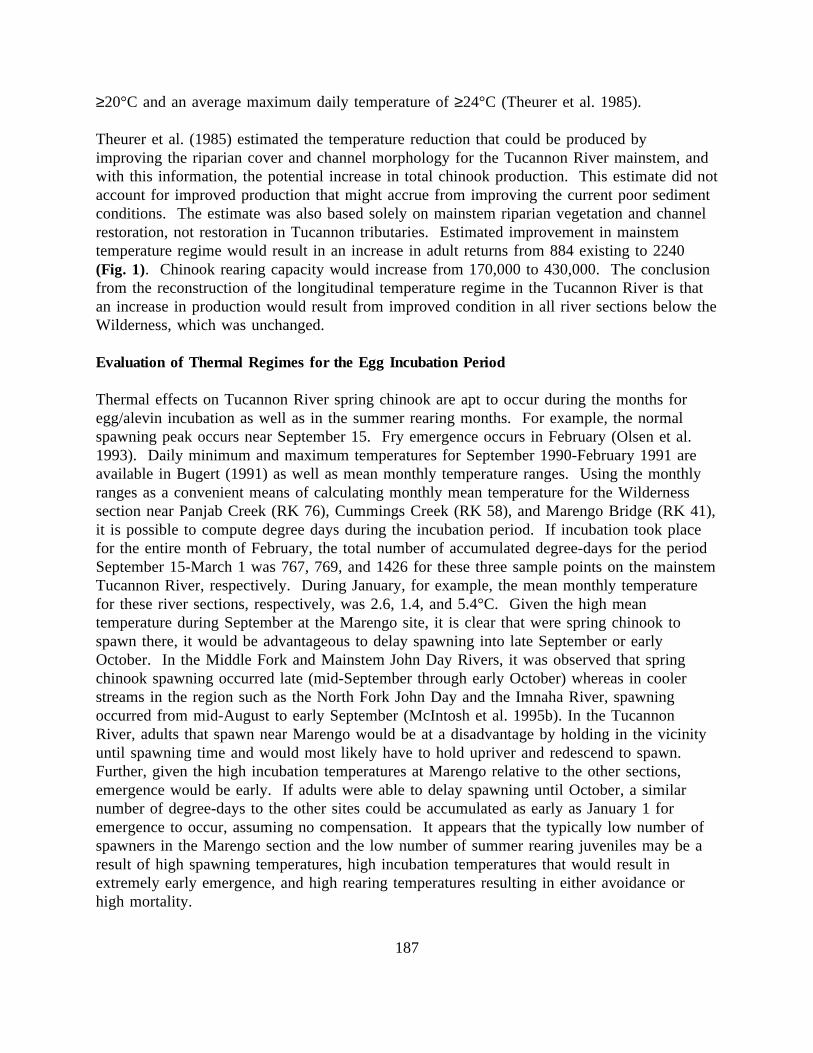
≥20°C and an average maximum daily temperature of ≥24°C (Theurer et al. 1985).

Theurer et al. (1985) estimated the temperature reduction that could be produced byimproving the riparian cover and channel morphology for the Tucannon River mainstem, andwith this information, the potential increase in total chinook production. This estimate did notaccount for improved production that might accrue from improving the current poor sedimentconditions. The estimate was also based solely on mainstem riparian vegetation and channelrestoration, not restoration in Tucannon tributaries. Estimated improvement in mainstemtemperature regime would result in an increase in adult returns from 884 existing to 2240(Fig. 1). Chinook rearing capacity would increase from 170,000 to 430,000. The conclusionfrom the reconstruction of the longitudinal temperature regime in the Tucannon River is thatan increase in production would result from improved condition in all river sections below theWilderness, which was unchanged.

Evaluation of Thermal Regimes for the Egg Incubation Period

Thermal effects on Tucannon River spring chinook are apt to occur during the months foregg/alevin incubation as well as in the summer rearing months. For example, the normalspawning peak occurs near September 15. Fry emergence occurs in February (Olsen et al.1993). Daily minimum and maximum temperatures for September 1990-February 1991 areavailable in Bugert (1991) as well as mean monthly temperature ranges. Using the monthlyranges as a convenient means of calculating monthly mean temperature for the Wildernesssection near Panjab Creek (RK 76), Cummings Creek (RK 58), and Marengo Bridge (RK 41),it is possible to compute degree days during the incubation period. If incubation took placefor the entire month of February, the total number of accumulated degree-days for the periodSeptember 15-March 1 was 767, 769, and 1426 for these three sample points on the mainstemTucannon River, respectively. During January, for example, the mean monthly temperaturefor these river sections, respectively, was 2.6, 1.4, and 5.4°C. Given the high meantemperature during September at the Marengo site, it is clear that were spring chinook tospawn there, it would be advantageous to delay spawning into late September or earlyOctober. In the Middle Fork and Mainstem John Day Rivers, it was observed that springchinook spawning occurred late (mid-September through early October) whereas in coolerstreams in the region such as the North Fork John Day and the Imnaha River, spawningoccurred from mid-August to early September (McIntosh et al. 1995b). In the TucannonRiver, adults that spawn near Marengo would be at a disadvantage by holding in the vicinityuntil spawning time and would most likely have to hold upriver and redescend to spawn. Further, given the high incubation temperatures at Marengo relative to the other sections,emergence would be early. If adults were able to delay spawning until October, a similarnumber of degree-days to the other sites could be accumulated as early as January 1 foremergence to occur, assuming no compensation. It appears that the typically low number ofspawners in the Marengo section and the low number of summer rearing juveniles may be aresult of high spawning temperatures, high incubation temperatures that would result inextremely early emergence, and high rearing temperatures resulting in either avoidance orhigh mortality.

187

Evaluation of the Relationship between Water Temperature, Air Temperature, and StreamDischarge

Water temperature is known to be correlated with air temperature. Stream discharge patternsalso affect the trends in water temperature. Periods of summer rainfall are associated withcloud cover and changes in air temperature and/or discharge. Changes in dischargecommonly produce opportunities for fish migration in various seasons. Data available fromthe Oregon Climate Service on air temperatures for LaGrande, Oregon were plotted withmaximum daily water temperatures for the Tucannon River at Cummings Creek for 1988 and1992. LaGrande is 125 km air distance from the Cummings Creek site. Periods of increasingair temperatures were typically linked with increasing water temperatures (Fig. 21). However,the rate of response to air temperature increases or decreases seems not to be the same duringall periods in the month examined.

For the year 1989, July-September maximum daily water temperatures were plotted in Figure22 along with the ratio of (maximum daily water temperature)÷(mean daily discharge). Again, air temperatures were those recorded for the LaGrande, Oregon station and watertemperatures were taken on the mainstem Tucannon River at the Cummings Creek site. These plots reveal a very close association between water temperature and the ratio. Thisrelationship appears to explain more of the variation in water temperature than is accountedfor by air temperature alone. It is interesting that a very substantial change in the T(air)/Qratio at day 54 in this 3-month period produced a corresponding change in water temperaturebut not as great as that produced by other smaller changes in the ratio. Despite thecorrelation between water temperature and air temperature and discharge, the key tomaintaining healthy salmon habitat is to delay the warming effect as far downstream aspossible. That is, one would expect a correlation between local water and regional airtemperature at all points down the river continuum. The correlation in the Wilderness reach,however, would be with a lower maximum daily temperature. In addition, one would expectthat local climatic (air temperature) conditions under the riparian canopy in this reach wouldbe responsible for the lower maximum daily temperature and would, itself, be correlated withthe regional air temperature.

188

RECOMMENDED STANDARDS

OVERVIEW OF THE PROBLEM

The process of developing temperature standards for salmonids in freshwater habitats is onerequiring great care and consideration. There are a variety of approaches that can be taken. For example, it is possible to base a standard or its application to a whole stream system on(1) the distribution of the species in its current range of habitats and the temperature limits todistribution, (2) suitable temperatures for what is considered to be the most sensitive lifestage, (3) suitable temperatures for single or multiple life stages, (4) effects on survival only,or (5) effects on a variety of life processes and activities such as avoidance, preference,growth, reproduction, migration, disease, feeding, territoriality, and aggressiveness, in additionto survival. These are all valid biological considerations. As matters of policy, there areseparate issues of whether (1) a species would be protected fully or partially throughout itsrange, (2) all native coldwater species would be protected on an ecosystem basis withinsubbasins designated as coldwater beneficial uses, and as a subset, or (3) whether native fishhabitats would be spatially linked or disconnected fragments. In response to both biologicalrequirements and policy decisionmaking, it is necessary to formulate a means of identifyinglevel of suitability or protection. Does full protection mean being able to fully occupy allhistoric habitats within the historic range of the species? Under these conditions, wouldsurvival be the optimum for a life stage under the dynamic geomorphic, vegetative, andclimatic processes that historically occurred? Would certain habitats be bottlenecks toproduction and population viability on account of quantity, quality, and spatial connectedness? As a matter of land management, will land management standards be developed so that watertemperature standards can be met? (See Rhodes et al. 1994 for an explanation of the linkagesbetween land management and stream processes and McCullough and Espinosa 1996 formonitoring protocols). In this process there are decisions to be made concerning whetherland management is to be conducted on an ecosystem basis or on a more reductionistic basis,such as focusing protection on key sites and dominant portions of the watershed (e.g., riparianzones). It must also be decided whether the standards that apply to biologic criteria and landmanagement practices would incorporate margins for error in estimation of biologic effectsand management outcomes and the natural stochasticity of environmental processes. Thealternative is that species' habitats would be managed as close to the brink of serious declineor extinction as possible to maximize all other resources having conflicting impacts to fishhabitat.

It could be instructive, in discussing all possible approaches to standards, to review the manyways in which freshwater temperature regimes have been perturbed in recent development ofColumbia River subbasins. The management activities (e.g., riparian harvest, wetlanddraining or filling, diversion of groundwater flows by road cuts) that have been responsiblefor the existing spatial patterns of alteration to thermal regimes suggest both the possible

189

mechanisms for impact to salmon populations and life histories (see Rhodes et al. 1994) butalso the logical means to monitor and summarize data on environmental quality (seeMcCullough and Espinosa 1996). It would also be worth reviewing our past processes formanaging land and monitoring and regulating water temperature to understand why theseactions have led to an ever shrinking quantity of available coldwater habitat for salmonids. The reasons for continued erosion in habitat quality undoubtedly are a combination of factors:complexity and difficulty in understanding all the biological effects involved, the tendency toallow degradation of water quality as a ready compromise in deriving non-aquatic benefitsfrom a watershed, and political difficulty in coming to grips with the geographic scope of theproblem, and resistance to fully believing or using what the scientific community hasprovided. Among the positions taken by various managers, regulators, the public, orsometimes by scientists themselves that have contributed to failure to halt the continuingthermal pollution problem are:

It is good to open up the canopy because the water temperature in streams of thePacific Northwest is too cold. Salmonid abundance and growth rate improve whenwater temperature increases.

Salmon endemic to streams of eastern Washington and Oregon are adapted to warmerwater temperatures than those endemic to streams west of the Cascade Mountainsbecause the climate is warmer on the eastside. These inherent differences in tolerancemake it ridiculous to apply a uniform standard state-wide.

Increasing the water temperature might be disadvantageous to one salmonid speciesbut it would merely improve conditions for other salmonids.

If water temperature in a stream reach attains upper lethal levels for a salmonid, this isnot a problem as long as the temperature cools off at night.

Salmonids have been observed in streams having very warm temperatures, proving thatin some locales these species have very different water temperature requirements.

As long as the mean daily temperature is within the range of temperatures that asalmonid species has been shown to tolerate in short-term laboratory tests, there willbe no effects on the individual or the population.

Laboratory tests on temperature preference or lethal limits do not apply under fieldconditions, so cannot be used to set temperature standards.

There are numerous thermal refugia in streams so there is seldom a problem for apopulation maintaining itself during warming periods.

Just because salmonids prefer cold water in thermal gradient experiments, that doesnot mean that they will not do well under warm water conditions. Densities of

190

salmonids appear to be high in warm water.

Much of the literature used to develop temperature standards is for salmon stocks notin the Columbia Basin, so is irrelevant. We need to do much more research beforeconsidering stringent standards.

You seldom see the dead carcasses of fish in the river so the importance of diseasesand other indirect sources of mortality must be overblown.

For a stream reach supporting steelhead, spring chinook, and bull trout, it is possibleto monitor only one species as a management indicator species. Steelhead are presentin sufficient numbers so will make a good choice for indicator species.

No matter what the condition of the stream, coldwater refuges exist where there isgroundwater entering a stream, and this will support fish throughout any summerperiod. The fish merely need to seek out these refugia.

Devise a temperature standard for maximum allowable temperature but also allowimpacts in the headwater riparian zones that progressively move the point where thestandard is exceeded in an upstream direction.

Select a standard that is in the resistance zone (i.e., where mortality is a function ofexposure time) because any lower standard might not appear to be linked to heat deathor might be judged a priori to be physically infeasible to attain.

Stream environments are naturally heterogeneous and salmon stocks have evolved insuch physical uncertainty and can cope with it. Salmon do not always have optimumconditions under natural conditions, so optimum should not be a management standard.

None of these approaches above can be considered to meet the biological needs of a speciesor to maintain health of the freshwater ecosystem. They are only mentioned becausesometimes it is easier to see how to do things right when contrasted with the voluminoustendencies to do the opposite, whether that be through sheer management convenience or lackof sufficient information to make a good decision.

As revealed in this review of thermal effects on salmonids, there are significant impacts tosurvival due to temperature regime worth considering in all life stages. In addition, there areother impacts considered to be sublethal on life processes such as growth, survival,reproductive success, migration success, disease, feeding, territoriality, aggressiveness,swimming, bioenergetics that cumulatively can result in diminished survival and production ofthe population. It is essential for anyone setting a temperature standard for any season orportion of a life history phase to thoroughly understand the breadth of control thattemperature exerts on population viability. When this is accomplished it is up to landmanagers to also fully consider the impact of their actions in an ecosystem context on the

191

temperature regimes found throughout a stream system from headwaters downstream. That is,freshwater habitat protection involves full protection and restoration of all riparian areas (fish-bearing, non-fish-bearing, intermittent) as well as the entire watershed so as to support allprocesses contributing to habitat quality and quantity (including water quality) (Rhodes et al.1994, Henjum et al. 1994, Reeves et al. 1997).

SELECTION OF A STANDARD FOR A RIVER CONTINUUM

All species encounter adverse environmental conditions at the limits of their range (e.g.,latitudinal or within a stream system) and periodically within their normal home range withannual or seasonal variation in climatic events. For example, yellow perch distribution inNorth America corresponds to the 15.6°C isotherm for mean July air temperature to the north(Ryder et al. 1964) and the 30°C isotherm for mean maximum midsummer air temperature(Weatherley 1963) to the south. The 20°C isotherm for annual air temperature establishes thesouthern limit to lamprey distribution (see references cited by Potter and Beamish 1975). Smallmouth bass are restricted in northward distribution by the 18°C isotherm for mean Julyair temperature (Inskip and Magnuson 1983). These air temperature indices correlate wellwith general fish distribution because of the linkage between air temperature and watertemperature (Hokanson (1977). However, within a river system, temperature regime varieslongitudinally with stream order (also correlated with width and elevation) and is modified bymanagement perturbations to channel width, riparian canopy cover, pool volume, watershedrunoff timing, and instream flow (Rhodes et al. 1994). Downstream limits to fish distributionhave often been linked to maximum temperature attained in the reach. For example, brooktrout are limited in downstream range to water temperatures <19°C (McCormick et al. 1972). The point in a stream system where this threshold is reached is, then, an outcome ofmanagement influence on the inherent temperature regime.

Maximum monthly or annual water temperature typically increases gradually in a downstreamdirection on a river continuum. Other key indices of the temperature regime likewise varylongitudinally. For example, the rate of degree day accumulation during the winter eggincubation period also changes in a downstream direction, leading to variation in emergencedate and duration of the emergence period. Timing of spawning must also coincide with theincubation temperature regime so that proper development time is allowed for emergence tooccur before adverse high springtime temperature. Salmonid species exhibit considerablevariation in life history patterns to accommodate the patterns of temperature regimes foundalong the river continuum. Management of the spatial array of thermal regimes found in thesystem of linked stream reaches can be simplified by ensuring that management impactsdistributed throughout a watershed do not interfere with the ability of coldwater fromheadwaters or from groundwater sources to flow downstream to the greatest extent beforereaching equilibrium with air temperature. A successful river management program wouldseek to provide optimum conditions to the extent that they are characteristic of theunmanaged, native state of the particular river segment. Obviously, not all reaches in a riversystem can be at optimum temperatures for every month for each fish species inhabiting thestream system. Summer months are vital to juvenile rearing and temperatures above the

192

optimum, which are increasingly found in downstream reaches, result in reduced individualgrowth rates, reduction in population net biomass gain, increased mortality rate, reduction inpopulation density, and eventual elimination of the species. Documenting the occurrence of afew individuals in a downstream reach does not allow concluding that the temperature regimefor the reach is adequate. Rather, if a threshold maximum temperature is exceeded, there isreason to determine whether all management actions upstream have been taken that wouldresult in restoration of natural cooling or thermal buffering processes.

In the management of coldwater fish species, the greatest degree of expression of life historyvariation by species is achieved by restoration of the thermal regime on a stream system-widebasis, along with other pre-management conditions of channel morphology and the watershed. Moving the summer maximum temperature threshold upstream constricts the availablespawning or rearing area of all coldwater fish species. Fish zonation from headwaters todownstream reaches in the Pacific Northwest can be characterized roughly as proceeding frombull trout/cutthroat trout to steelhead, to spring chinook/coho, to summer chinook, to fallchinook, to chum (Li et al. 1987). With the exception of bull trout, the other species do notvary substantially in their response to summer maximum temperature. However, they do varyin their preference for size of spawning and rearing stream, size of spawning gravel, andstream gradient tolerated. Increase in summer maximum temperature in headwater streamzones cannot occur without causing increase to downstream reaches. Constraining speciesmore and more to compete in high gradient streams that may provide suitable watertemperatures would severely limit production and impair survival in the majority of thehistoric habitat of each species, but further, it is not feasible energetically for large-streamspecies to occupy smaller, high gradient streams.

Ideally management of watersheds could be done in such a way that historic temperatureregimes would be restored in all stream reaches throughout each stream system. Theurer etal. (1985) demonstrated that, given a large modeling effort, the restored longitudinaltemperature profile for summer months could be estimated under restored riparian vegetationand channel width for the Tucannon River mainstem. This model demonstrated that throughrestoration efforts focused on the mainstem that the lower 40 km of river could be madeinhabitable by juveniles during summer. It is likely that full watershed restoration (restorationof tributaries and their watersheds) would result in even greater production potential. Taylorand Barton (1992) recommended that the ultimate management goal is to restore naturalfrequencies of temperature exceedences with no perturbation by management influence. Theystate that management of frequency of temperature exceedence is needed to ensure thatpopulations living in marginal habitat are not further stressed. Populations living in marginalhabitat suffer high frequencies of temperature exceedence; increases in their probability ofexperiencing stress from temperature exceedence results in greater acute mortality.

Although the ideal may be to determine an historic longitudinal temperature profile andmanage the watershed to recreate this condition on average, this approach is not practicable. The data requirements for reconstructing historical profiles for all streams in the ColumbiaRiver basin would be severe. Gathering information on historic riparian condition would be

193

challenging in itself, but many other factors such as historic channel morphology, channelvolume, drainage density, and hydrologic conditions (e.g., linkages to wetlands orgroundwater) contribute effects to the thermal regime. Even with adequate knowledge ofhistoric conditions, precise modeling of these effects is unlikely. If an ideal longitudinaltemperature profile were created, it would represent a long-term average condition that wouldhave to be bounded by a probability density function. The most reliable means ofdetermining this profile with its frequency distribution at each point along the curve is not bymodeling but by restoring the watershed and then monitoring the profile for several years.

If this ideal profile and its frequency distribution were available as a standard, how wouldfuture monitoring take place to identify violations of the standard. There are a number ofalternatives that could be proposed. In one scenario, several years of data at points along theprofile would have to be averaged before it could be determined whether a significantdeviation from the historic mean occurred for each selected point along the profile. And thiscomparison of recent condition with baseline years of record implies a stationary climaticregime.

Another alternative is to monitor the maximum temperature at a point on the profile anddetermine where that value falls in the frequency distribution. Values in the upper 5thpercentile could be considered to be a violation because they are so rare one would not expectthem. The "range of natural variability" is sometimes used to determine acceptability of aresource condition. That is, values that occur within the 5th and 95th percentile of historicnatural conditions could be considered normal. Unfortunately, this method is fraught withconceptual problems that render it unusable (Rhodes et al. 1994). If maximum watertemperature were at the 6th percentile level for annual maximum temperatures, one could notknow whether this occurrence reflects part of the natural historic distribution or a newdistribution shifted toward higher mean temperatures unless more years of data werecollected. At this point, unacceptable damage could be done. Ironically, another variation tothis theme proposed in the recent revision to the Oregon temperature standards was to excusethe extreme temperature values as basically acts of God. With these two concepts in tandem,one would accept the center of the distribution as within the range of natural variation and theextremes as acts of God.

One other alternative for determining temperature violations from a single year of data wouldbe to first assess where the maximum temperature occurs in the ideal distribution for aparticular point on the profile and then to determine whether this extreme was predictable. That is, if under the desired future watershed/riparian conditions it would take a high airtemperature, full sun, high humidity, low wind speed, and high maximum water temperaturefor the previous day to produce a 1°C temperature exceedance at a particular point on theideal profile, but under current conditions such an exceedance occurs under more benignconditions, one would conclude that management changes need to occur. Although thismethod would be effective, we do not typically have a complete knowledge of historicconditions, historic temperature profiles and their frequency distributions, or adequate currentenvironmental data with which to predict temperatures. Even with abundant data of this type,

194

predictions on a stream network basis are not highly accurate.

Use of a single maximum temperature standard for an entire watershed is often ridiculed as a"one size fits all" standard. Recommendation of such an approach though does not imply thatall watersheds are created equal but that each species that we manage has relatively uniformwater quality requirements. In practice, the management response to detecting a variationfrom the historic longitudinal profile would be the same as in managing according to a singlebasin maximum temperature standard. That is, if the recent multi-year mean of annualmaximum temperatures were greater than the historic mean of annual maximum temperatureswithin a particular reach, management actions within the reach and in the upstream watershedwould have to be modified. The minimum requirement for restoring the historic profilewould be to allow for passive restoration of all riparian zones and channel morphology in thestream network. To hold that less than full riparian restoration can be done means, as aminimum, that one is content with marginal improvement or a fraction of full fish productionand that the responsibility can be borne by some landowners but not all. Of course, simplyfocusing efforts on the riparian zone (and maybe even a small riparian buffer not functionallycapable of reducing solar input or shaping channel morphology) is not sufficient. Maintainingand restoring wetlands and other sources of cold water and rearing area are significant as arereduction in road density and other watershed measures. One thing that a well describedhistoric longitudinal temperature profile could do very well if it were ever feasible would beto alert regulators to local deviations from the desired profile, especially in the upperwatershed areas. This is the location where cold waters might be warmed significantly, but tolevels below optimal. It is important not to incur widespread warming of headwater streams. This effect would be detected at some point downstream, but then the task would be to takecorrective action later to address all cumulative upstream landscape alterations that led to thisproblem. Because the ideal profile tends to reach an asymptote far downstream whereequilibrium with air temperature is attained, this is not the most sensitive site for monitoringtemperature. The greatest deviations from the ideal profile occur upstream, and this is wherepreventive actions need to be taken.

Averaging annual maximum temperatures in a reach over a 20-year period to compare it withan ideal profile describing the historic mean would require too long a data collection periodbefore corrective actions could be taken. Any individual year could have an annual maximumtemperature that exceeds the long-term natural profile. It would not be feasible to determinewhether an annual exceedance is natural or has a management-related cause withoutattempting to correlate the annual maximum with annual air temperatures and account for allantecedent air and water temperatures, variations in groundwater input, etc. (see Stonemanand Jones 1996). Obtaining a long (e.g., 20-year) record of temperatures in order to estimatethe statistical likelihood that temperatures are attributable to natural rather than managementcauses does not allow timely adaptive management. It is far more direct to addressmanagement actions known to lead to temperature increases than to attempt temperaturereconstruction and estimations of probabilities.

195

In conclusion, use of a single maximum summertime water temperature as a management toolis as useful as knowing the historic longitudinal profile because the response to exceedence isthe same. That is, exceedence of the threshold maximum temperature would cause upstreammanagement actions to be modified if they were found to be impairing the ability of theriparian zone to achieve its natural vegetative cover and to control channel morphology. Aspreviously stated, other watershed functions must also operate so that natural water andsediment delivery regimes are maintained. Exceedance of the temperature standard is thetrigger to initiate adaptive watershed management. However, no temperature standard, evenone fully linked in technical documentation to its biological consequences, can force landmanagers to recognize or address the effects of management actions on water temperaturewhen there is an unwillingness to do so. Basically, the physical principles of stream heatingare well known. Actions that cause temperature increases are well documented (Rhodes et al.1994). Predicting the exact magnitude of increase is more difficult but it is seldom contestedthat cumulative reduction in riparian canopy cover for a stream system cumulatively warmsstreams.

If it is concluded that a single maximum summertime temperature should be the statistic usedto identify a potential stream temperature violation, one must decide what the exacttemperature should be. One alternative is to choose the temperature that finally results inelimination of the species from the stream. For a wide variety of salmonids, maximumtemperatures of approximately 22°C-24°C have been shown in the literature to result in alimit to distribution. Fish species are typically eliminated by temperatures less than theirUILT (Hokanson 1977). McCormick et al. (1972) found brook trout distribution to be limitedto temperatures <19°C. This threshold for species presence was also close to the zero netgrowth temperature of 17.9°C. It appears that the field limit to distribution is a temperaturebetween the ZNG temperature and the UILT. Setting this temperature (approximately 22°C-24°C for spring chinook) as a maximum instantaneous temperature standard would serve littlepurpose as a management tool. If all stream reaches were increased to the standard, thespecies would be eliminated throughout the stream system. It makes far more sense to set thegrowth optimum as the standard. For spring chinook this is approximately 15.6°C. Duringthe summer, temperatures less than this cause no reduction in survival, whereas temperaturesgreater than this begin to reduce growth and lead to increasing mortality rates. Monitoringstream temperature in stream orders 4-6 would allow comparison to the maximum allowabletemperature. Exceedance in any of these monitoring locations would require evaluation ofmanagement practices upstream. If maximum temperatures were limited using properwatershed management, amplitude of diel fluctuation would also be limited, as wouldfrequency of exceedence of the maximum. Restoration of stream temperatures in the springchinook zone would require restoration of conditions producing cold water throughout thedrainage; this should ensure that the even lower maximum temperature requirements for bulltrout are met in lower order streams. However, even though temperatures in the mainstemare influenced by cumulative impacts in headwater streams, significant biological damage canoccur in the headwaters before an increasing temperature trend is detectable in the mainstem. Consequently, for protection of the local bull trout/cutthroat trout populations to be full andfor cumulative effects to the mainstem fish populations to be minimized, full protection of all

196

processes delivering coldwater must be maintained. Assuming a longitudinal zonation frombull trout and cutthroat trout in headwater streams to spring chinook and steelhead in streamorders 4-6, it would be probable that in terms of temperature alone, if bull trout habitat is inoptimal condition throughout its range, the opportunity for spring chinook and steelheadhabitat to have optimal conditions is great. Such a management scenario would representecosystem management at its best.

197

SUMMARY

HISTORICAL BACKGROUND

The Federal Water Pollution Control Act, amended in 1965 as the Federal Water Quality Act,called for standards to be established for protection and enhancement of water quality inwaters of the US. In 1968 the Columbia River Thermal Effects Study was begun in responseto adoption of temperature standards by Oregon and Washington that were inconsistent withone another. This study was authorized by the US Secretary of the Interior. In 1970 theNational Marine Fisheries Service (NMFS) was created within NOAA to replace the Bureauof Commercial Fisheries in the Department of Interior (DOI). Also in 1970, EPA wascreated, replacing the former Federal Water Quality Administration and was given authorityfor overseeing environmental protection, including water quality. In January 1971 EPA incooperation with the Atomic Energy Commission (AEC, represented by Battelle Northwest)and NMFS released the publication entitled Columbia River Thermal Effects Study. Results of51 new studies on biological effects were reviewed in this publication in addition to muchsignificant past research. The studies completed for this review included research conductedby the Federal Water Quality Administration, NMFS, and the AEC.

Impetus for this review came also from perceived changes in the Columbia River system. The upriver runs of Columbia River fish resources have been reduced and endangeredby the physical alteration and blockage of migration routes by the Nation's largestsystem of dams and reservoirs. The quality of the aquatic environment has also beenmodified by the discharge of pollutants and impoundment of the river's flow in aseries of reservoir lakes reaching into Canada. Particularly regarding temperaturequality, the Columbia River temperatures have been both spatially and temporallyaltered by man's activities and use of the water resources of the Region.

There was at this time increasing concern for numerous point source discharges of heatedpower plant effluents.

Today, 27 years later it is clear that temperature control on the mainstem and tributaries ofthe Columbia River is of even greater concern. The historic thermal regimes have beenaltered on a geographically extensive basis by a history of land management decisions andland uses. Many ongoing activities continue to inhibit thermal restoration and new activitiesthreaten to worsen the thermal regime, moving the stream zone at which salmonids are finallydisplaced by high summertime water temperatures further and further in an upstreamdirection. In addition to point source discharges, it has become obvious that extensivenonpoint source thermal pollution is also a significant problem. Recent progress has beenmade in understanding the spatial distribution of temperature within the Columbia Riverreservoirs (Fryer et al. 1998) and the ability to modify reservoir temperatures through releasesof cold storage water (Karr et al. 1992). In 1971 the field of restoration biology was not

198

recognized, but today practical experience has been gained in bringing about basinwidereductions in stream temperature through riparian recovery (e.g., Hostetler 1991); predictionsof thermal recovery potential have also been made by use of stream temperature models ontributaries (Theurer et al. 1985, Chen and Chen 1993).

Monitoring of tributary water temperature today has become much easier with the advent ofcheap, digital thermographs whose data can be readily downloaded to computers. This hasincreased the spatial extent of monitoring and a greater appreciation of the magnitude ofthermal alterations to the region's waters. Increased monitoring of temperature of waters ofthe Pacific Northwest has led to listings of hundreds of streams as water quality limited, thatis, no longer fully providing beneficial uses. At the same numerous species have been listedas threatened or endangered under the ESA. Fish runs that are cause for concern, leading tothe EPA and NMFS report, are generally in far worse condition today. Although waterquality is not responsible for all listings, it is certainly influential as a factor limitingproduction potential, distribution, and survival in streams of the Columbia River Basin. Elevated water temperature is probably the single most significant water quality factorlimiting salmon survival.

In all temperature criteria adopted in the PNW, maximum upper limits were set for streams. Theoretical concepts of maximum thermal limits arose from pioneering work of Fry et al.(1946), Fry (1947), Hart (1947, 1952) and Brett (1952). This and other work was latersynthesized by Coutant (1972) in an EPA handbook that differentiated ideas about allowableshort-term exposure and long-term exposure. The methodology for estimating upper incipientlethal temperature (UILT) incorporated concerns about short-term exposure. Today, there isconsiderably more understanding of effects of long-term exposure, sublethal, indirect,cumulative, and synergistic effects, and the impacts of these effects throughout the salmon lifecycle.

The process of setting temperature criteria requires evaluation of the biological needs of allspecies utilizing a watershed. In the Columbia River Basin, streams in the current or historicrange of anadromous fish are designated as having a coldwater beneficial use (unless the usewas specifically downgraded), although there are also trout streams in non-anadromouswatersheds. Satisfying these uses involves satisfying the needs of the most sensitive species. Among the Salmonidae, the most valuable coldwater-dependent fish resource, there is a smallamount of variation in thermal sensitivity among species, with bull trout being highlycoldwater-dependent and the salmon being somewhat more tolerant of higher temperatures. Redband trout are considered to be the least dependent on cold water. Nonetheless, all thesesalmonids are coldwater species and their distributions generally follow longitudinal patternsof water temperature increase from headwaters downstream. This distribution pattern ofsalmonids is linked to the natural pattern of downstream warming of streams. In addition,distribution is related to the species' requirements for channel gradient, spawning substratesize and condition, pool frequency and quality. Abundance of a species tends to be related toall these factors, but is also influenced by numerous other habitat factors, such as waterchemistry, large woody debris frequency and abundance, bank condition, etc. Proper water

199

temperature, however, is a vital need for both distribution and abundance. If the water is toowarm in any stream reach, it does not matter how good any of the other habitat factors mightbe. In an ecological management sense, salmonids of all species would find the best matchbetween needs for cold water temperature and all other habitat factors mentioned providedthat the watershed is managed in such a manner to allow cold water to flow downstream tothe greatest extent before becoming too warm to be useful to salmonids.

The process of setting water temperature standards requires first identifying the most sensitivebeneficial use. Salmonid spawning and rearing tend to be uses that require water that is ascold as physically feasible from the watershed involved. Temperature criteria have been setutilizing various basic information, such as the UUILT, the optimum temperature, finalpreferred temperature. Criteria set by regulatory agencies have used formulas such as MWATthat incorporate policy decisions to allow a certain amount of warming beyond the optimaltemperature. They can also rely on assumptions that safety factors of a certain magnitude areadequate to keep a fish population from getting too close to a threshold temperature, beyondwhich negative effects become increasingly severe. Temperature criteria can also be basedupon optimal conditions, because it is known from experimentation that survival, growth,reproductive capacity, scope for activity, disease resistance, etc. are best under theseconditions. Because the effects of warm water are much more completely known today thanin 1971, especially of sublethal effects, there is today a more compelling basis for managingfor optimal conditions. In terms of providing a summary of this report, critical quantitativeinformation can be found in figures and tables, such as the figure illustrating the temperaturecriteria for spring chinook. Tables are also presented on UUILT and CTM values for variousspecies. The greatest value in this report, however, is not in statistical information but in theconcepts and their biological basis that can be used in conjunction with thermal responsestatistics to support maintenance and restoration of optimum conditions. A temperaturethreshold provides the target (e.g., an optimum temperature for an activity), but the conceptsstemming from all research available on biological effects provide the impetus for managingstreams and their watersheds to achieve the target, and to manage with clear conviction andintent.

THE CURRENT DOCUMENT

This document provided a review and analysis of thermal effects reported in recent literature,as well as some of the most significant older literature upon which most of our presentconcepts are still based. The 1971 Columbia River Thermal Effects Study provided a majorsynthesis of research available on effects to salmon in the Columbia River. The ideaspresented in this report were very comprehensive and could easily have been sufficientdocumentation to support stringent actions to control water temperature increases. Forwhatever reason the numerous concepts presented in this report did not appear to be takenseriously in the field of temperature regulation. Possibly the reason for this was apreoccupation with investigation of damaging effects of power plant effluents (point sources)or maybe because the emphasis was on the mainstem effects rather than tributaries it wasbelieved at the outset that little could be done to improve the thermal environment with the

200

system of dams in place. In any case, the current review substantiates the positions held inthe previous document, amplifies many of its points, and adds considerable new informationand conceptual material from the recent literature that makes the need for action even morecompelling.

The main messages in this document can be summarized in contrast to what was available ornot available in the Thermal Effects Study (TES). The TES had physical and biologicaleffects components. Physical measurement and analysis of river temperatures provide themonitoring data for expressing the state of the environment and indices to potential biologicalimpacts. In the TES water temperatures were measured with chart recorders. Currently, thecapability of monitoring water temperature has increased dramatically with inexpensive digitalrecorders that allow data downloading to computers for analysis at programmable timeintervals. A new device, forward looking infra-red (FLIR), allows thermal scanning of entirestream surfaces where not blocked by riparian canopy. These instruments working in tandemprovide a powerful means of performing rapid, extensive surveys. In 1971 the influence ofmainstem dams in altering the distribution of heated waters both spatially and temporally wasknown. Research indicated a shifting of high water temperature into the autumn period and aloss of the normal daily fluctuation with the reservoirs in place.

Prior to 1971 experiments were undertaken to release water from Grande Coulee to lowerHanford Reach water temperatures. In recent years releases from Dworshak Reservoir wereconducted to demonstrate a lowering of Snake River water temperature. The TES conductedmodeling of river temperature for water management. The recent development of numerousmainstem and tributary temperature models allows prediction of temperature under riveroperation conditions with expected tributary inputs and also tributary temperatures based onchannel morphology and riparian condition and other physical factors.

Biological effects were the main focus of this document and Volume 1 of the 1971 report. Numerous thermal effects on adults were recognized in the 1971 report. It was recognizedthat adults of any species have been observed to spawn within a fairly extensive temperaturerange but that for any species there is an upper and lower limit beyond which spawning isincreasingly inhibited. It was known that high water temperature subjects adults to increasedrate of disease and a higher metabolism that can easily deplete energy reserves. Adults enterthe Columbia River with an initial energy supply that is largely exhausted by the timespawning is complete. Adults were known to use thermal refuges to escape high watertemperature. Elevated water temperature can cause migration blockages. Sonic tagging offish indicated a complex migration pattern of individual fish, with actual distance travelledbeing much greater than the net distance to spawning grounds. The effects of disease onadults were studied intensively, especially the incidence and survival rates of columnarisinfections. It was known that warmwater diseases in general increased in terms of percentagemortality and virulence with temperatures beyond a threshold of approximately 15.6°C. Itwas also learned that adult salmon have a substantially lower thermal resistance (UILT of 21-22°C) to elevated temperatures than do the juveniles, making it dangerous to set temperaturestandards on the basis solely of juvenile exposure research.

201

Today bioenergetic studies are available that reveal energy allocation to growth, respiration,swimming, and other activities. Managing water temperature to provide optimal scope foractivity helps ensure that adults will not have stress levels so high that there is little energyavailable for disease resistance. It has been well documented that temperatures ofapproximately 21-22°C establish migration barriers to most adult salmonids. Delays inmigration that have been observed are significant enough so that the probability of survivingto spawn or to reach spawning grounds in time to spawn becomes low. The importance ofcoldwater refuges has been well documented using radiotracking devices. In addition, it hasbeen found that coldwater refuges themselves are typically small in surface area and theiravailability (frequency and size) can be compromised by management actions. For example,loss of LWD, sedimentation of primary pools, channel widening, increases in road density,and loss of wetland habitats can lead to reduced inflow and retention of cool groundwaterbottom areas of the channel. Migration patterns are increasingly well understood, usingradiotracking equipment. Complex migration routes are observed in different portions of arun. Adding thermal blockages imposes delays in migration and also tends to lengthen themigration paths by increasing exploration and retreat behavior in which fish seek cold refugesand avoid warm water zones, followed by attempts to seek natal spawning grounds later undercooler conditions. There is currently much greater understanding of the effects of elevatedtemperatures in controlling the infection rate and course of warmwater diseases. Thepercentage survival and the time to death from the point of infection both decrease withincreased temperature beyond the disease threshold. A great increase in understanding of theimportance of prespawning temperatures occurred after the TES study. Effects on adultsoccurred as thermal death, increased disease, inability to migrate, and inhibition of spawning. In addition, elevated temperatures cause reduction in gamete production and viability. Evenwhen fertilization occurs in warm waters (especially waters >16°C) delayed mortality isobserved as well as growth abnormalities.

The egg stage was known in 1971 to be a sensitive stage in development. As a general rule,salmonid eggs are sensitive to water temperatures <4°C and >14.4°C. It was found that eggscould withstand temperatures approaching 0°C if they were presented after the 128-cell stageof development. The ideal egg incubation temperature was considered to be approximately5.5-12.8°C for all salmon species, although tolerance to temperatures as high as 18°C wasthought to occur in some species in fluctuating temperature regimes. Diel temperaturefluctuations were thought to be beneficial during incubation as opposed to constanttemperature incubation.

Today a vast increase in information on the thermal effects on eggs is available. The rate ofegg development of all salmon species with temperature is highly predictable. In addition,data on survival rates for eggs incubated at temperatures <4°C and >14.4°C are available. For almost all salmonids these temperature thresholds remain as meaningful guidelines forobserving impacts of higher and lower incubation temperatures on survival. There are somestatistically significant differences among stocks and families within stocks in survival at lowand high temperature ranges. However, in terms of absolute degrees temperature thedifferences tend to be small. Salmon stocks from inland populations tend to be adapted to

202

colder winter conditions and those from coastal populations are better able to withstandwarmer winter incubation temperatures. This can be attributed to the more moderate thermalconditions in coastal streams than interior streams. Stocks that are more thermally tolerantthan others tend to have less capability for any further selection of tolerance characteristics.

In terms of egg incubation temperature it is reasonable to establish maximum allowabletemperatures at egg deposition stage. Excessive temperatures reduce egg viability andfertilizability. However, just as important as meeting critical threshold temperatures atdeposition is accumulating the required number of thermal units during development. Theentire thermal regime during the incubation phase is important to the proper timing of fryemergence. That is, even though temperatures of 10°C would provide high survival toemergence, the greater rate of development would lead to very early emergence. Development times under fluctuating thermal regimes during incubation can be estimatedfrom mean temperatures. However, compensation has been documented as a mechanism thattends to help maintain emergence at a prescribed number of days incubation, despite variationin temperature, within tolerance limits. Emergence times can be predicted by using meantemperatures for a sine wave thermocycle or also by using an egg development rate equationat each time increment during the cycle and calculating the percentage of a full developmentto emergence period that is completed at each increment.

In 1971 it was known that thermal effects to fish (and especially to juveniles, because mosttest fish were juveniles) were a function of thermal dose, which was related to time andtemperature of exposure. Also, the resistance time to constant temperature exposure is afunction of the prior acclimation temperature. In the field, fish are acclimatized to a certaintemperature regime and the thermal response to elevated temperatures depends on this historyof exposures and also on other factors, such as health, condition, size, age, etc. Upper andlower exposure limits were described for all salmon as well as preference temperatures in thework of Brett (1952). Studies of the effect of temperature on growth resulted in establishingoptimum growth ranges, beyond which growth rates decline significantly. Knowledge of theoptimum temperatures and the lethal limits led to establishing criteria to protect fish. Temperatures of >17°C were cited as leading to increased risk of disease. In addition, hightemperatures were discovered to be linked to increased predation risk. Thermal shocks alsowere found to produce greater predation risk. Repeated exposure to lethal temperatures forsublethal times were not considered to have an effect. However, exposure to multiple stress,such as temperature and heavy metal toxicants was found to reduce resistance times.

Since 1971 a great amount of new information has become available on juvenile effects. TheUUILT of most salmonids falls within the range 21-26°C. However, it seems clear that directmortality can be produced from single exposures or in cumulative exposures over a series of2-3 days, resulting cumulatively in 100% of a lethal dose. Temperatures above 24°C becomeincreasingly significant in adding to a lethal dose. Using constant temperature experimentalresults, the time to death can be predicted from increments of temperature above 24°C onsingle or multiple days exposure. Because fish in the field are acclimatized to temperaturesexperienced over days preceding a critical exposure, it is problematic to estimate what the

203

effective acclimation temperature is. Experimental work has revealed that effectiveacclimation temperature in a thermocycle tends to be equivalent to a temperature between themean and the maximum of the cycle. Most work indicates acclimation either to atemperature midway between the mean and the maximum or to the maximum.

Although salmonids can be excluded from a stream reach by lethal temperatures they can alsoleave voluntary due to thermal preference. Intrabasin migration has been well documented insalmonids and allows juveniles to move to temperatures more nearly meeting preferences. However, migration barriers, thermal barriers, limited area of coldwater refuges, or inability toswim the distances needed to retreat to cold water all can lead to exposing a portion of thepopulation to thermal death under warming stream conditions during the season. On a multi-annual basis continued riparian cover loss leads to overall restriction in productive capacity ofthe stream. Despite the upper lethal limits, fish tend to be limited in distribution to uppertemperatures in the range 22-24°C. That is, the downstream limit to distribution tends to be2-3°C less than the UILT. This temperature range establishes the point on the mainstem of atributary at which salmonids make the transition from present to absent. Population densitydeclines to zero in this zone. Upstream of this zone temperatures are typically colder, and astemperatures enter the optimal range under other optimum habitat conditions (e.g., gradient,pool frequency and quality, etc.), population density can reach an optimum (this is a highlysimplified concept because carrying capacity involves many more factors, see McCullough1996). Fish survival is not impaired by summer cold temperatures, but growth rates could below in certain streams, requiring an extra year of development to emigrate (anadromous) or tomature (resident).

Growth rates in the field are a useful index to optimal temperatures. Survival rates are highunder these temperatures, but at the growth limit, increasing stress occurs. Very significantinformation was provided in studies on sockeye by Brett (1971, 1983) and brown trout byElliott (1971, 1994), showing that as food becomes limiting, optimum growth temperaturesdecline. Typically under field conditions fish are not able to feed to satiation so growth ratesare seldom as high as might be predicted from constant temperature experiments undersatiation feeding. At the same time as food supply diminishes, loading stresses influencesurvival at lower temperatures. Many studies have related growth rates in the field underfluctuating temperatures with growth rates in the laboratory under constant temperatures equalto the mean temperature in the fluctuating regime. Some studies have concluded that there isno difference in growth rates among populations in different environments under similar meantemperatures in a fluctuating regime and consequently no genetic differences. Other researchimplies that growth rates in fluctuating temperature regimes are greater than under constanttemperature regimes.

Genetic differences in growth rates are sometimes demonstrated among stocks reared atconstant temperatures, but they are frequently only evident at the extremes in temperaturewithin the tolerance range of the species. Certain stocks are found to have somewhat greaterresistance times to extreme temperatures than other stocks, but most typically, whendifferences occur they are associated with morphological differences and with differentiation

204

as subspecies. The absolute differences in resistance times are small and do not ever result ina conclusion that higher critical levels should be established for certain stocks.

Bioenergetics and power budgeting are important new ways to view the energy allocationsmade by fish to accommodate their growth, metabolism, and activity needs. The scope foractivity is a function of acclimation and exposure temperatures in the same way as lethalresponses. The greater the scope for activity under a combination of acclimation andexposure temperatures, the greater is the ability of the fish to perform burst swimmingactivity to negotiate falls or escape predators. Also, if the fish is able to maintain a largescope given its exposure temperature regime, it is more able to resist disease. Powerbudgeting is energy allocation made under very short time periods (seconds to minutes). High levels of exertion requiring long periods of rest result in short-term inability to performother functions necessary to survival. Bioenergetics can be considered as the long-termallocation of energy resources to perform life functions, such as migration and spawning. Storage of fat and protein prior to migration is essential so that the migration distance can betraversed, holding occurs, and spawning activity and nest guarding take place.

Much has been learned in recent years about role of temperature in mediating the outcome ofcompetitive interactions between fish species. Overlap in habitat use is established bypreference for factors such as channel gradient, depth, substrate composition. Given aresource used in common, the outcome of competition is typically related to size andaggressiveness. This is frequently reported in studies of competition among salmonids. However, temperature is very important in shifting competitive dominance between twospecies having different thermal preferences. In competition between salmonids andcoolwater tolerant species, this transition in dominance occurs 2-4°C lower than the range ofmaximum temperatures that is usually associated with total elimination of salmonids in a rivercontinuum (i.e., 22-24°C).

Synergistic effects on salmonid survival are much more adequately understood today than in1971. Temperature combined with numerous other water quality factors, such as dissolvedoxygen, suspended sediment, heavy metals, and cyanide, effectively reduces the resistancetime to death at a certain temperature, or conversely results in 50% mortality within 24 h at alower temperature. Synergistic effects have been well studied on juvenile survival, but theirimpacts are also documented as causing migration delays in adults and egg mortality inspawning gravels.

The TES report provided some information on smolt migration under the influence of thermalexposure. It was known that due to the effect of dams the rate of migration to the ocean wasreduced. Premature or delayed entry to saltwater reduced survival. Warm water in reservoirswas known to inhibit migration, increase residualism, predation risk, and disease occurrence. Thermal shocks that occur within and do not exceed the range 5-23°C were thought not toimpair swimming performance. A temperature range of 5-17°C was considered acceptable forsmolt migration.

205

Since the TES report many new studies became available concerning the influence oftemperature on smoltification. Dynamics of smolting involve the interaction of temperature,photoperiod, and the trend in both temperature and photoperiod. However, under fieldconditions photoperiod and the direction of change in photoperiod are not subject tomodification and altered temperature conditions become the primary means of impact to thesmoltification process. It has been learned that temperatures that become inhibitory tosmoltification for certain species can be as low as 13°C. Incomplete smoltification ordesmoltification caused by elevated emigration temperatures reduces the saltwater readinessand impairs their marine growth and survival.

206

FIGURES

207

Figure 1. Effect of temperature profile in the Tucannon River on spring chinook rearingcapacity and adult returns based on three restoration scenarios. Taken from Theurer et al.(1985) and a calculation of Jon Rhodes, CRITFC hydrologist.

208

0

500

1000

1500

2000

2500

3000

3500

4000

4500

0

500

1000

1500

2000

2500

3000

3500

4000

4500

0

500

1000

1500

2000

2500

3000

3500

4000

4500

0

500

1000

1500

2000

2500

3000

3500

4000

4500

Juve

nile

Rea

rin

g C

apac

ity

(x10

0)

Nu

mb

er o

f R

etu

rnin

g A

du

lts

Restored Existing 1.1 C increase

Figure 1.

209

Figure 2. Spring chinook temperature requirements.

210

J F M A M J J A S O N D J F M A M J J A S O N D0

5

10

15

20

25

AD

ULT

HO

LDIN

G

SP

AW

NIN

G

EG

G IN

CU

BA

TIO

N

FR

Y E

ME

RG

EN

CE JU

VE

NIL

E R

EA

RIN

G

DISEASE SPAWNING15.5

13.3

4.5

12.0

15.6

14.8

10.0

16.0

12.8

14.0

19.1

4.5

12.5

8.0

5.6

OPTIMUM

PRODUCTION

POSITIVE GROWTH

21.0

3.3

12.2

SMOLT LETHAL + LOADING STRESS

+ A

LEV

IN IN

CU

BA

TIO

N

12.8

18.3

41

50

59

68

77

TEMPERATURE TOLERANCE >1.7

ADULT MIGRATION BLOCKAGE 22.0

AD

ULT

MIGRATION SPAWNING INCUBATION EMERGENCE REARINGHOLDING

SM

OLT

IFIC

AT

ION

+ O

UT

MIG

RA

TIO

N

Spring Chinook Temperature Requirements

MAXIM

UM GROW

TH

OPTIMUM

PRODUCTION

POSITIVE GROWTH

FIRST FEEDING

DISTRIBUTION LIMIT

ZNG

ZNG

ZERO INDIV. GROWTH

UUILT 25.1

oC Fo

Figure 2. 211

Figure 3. Days from fertilization to emergence for chinook, coho, and sockeye salmoncalculated from formulas of Beacham and Murray (1990).

212

50

100

150

200

250

300

350

DA

YS

2 4 6 8 10 12 14 16

TEMPERATURE (CELSIUS)

CHINOOK COHO SOCKEYE

DAYS TO EMERGENCE

Figure 3.

213

Figure 4. Reduction in number of days to emergence for each 1°C increase from a basetemperature of 2°C, calculated for chinook, coho, and sockeye. Calculated from data plottedin Figure 3.

214

0

10

20

30

40

50

60

DA

YS

2 4 6 8 10 12 14 16

BASE TEMPERATURE (CELSIUS)

CHINOOK COHO SOCKEYE

REDUCED NO. DAYS TO EMERGENCEFOR EACH 1 DEGREE INCREASE FROM BASE

Figure 4.

215

Figure 5. Cumulative thermal units (degree days for temperatures >0°C) for spring chinookincubation periods in the mainstem John Day (RK 422) and the North Fork John Day (RK97) for years 1980-81 and 1982-83. Thermal units are plotted against days from peakspawning on the mainstem John Day. Data taken from Lindsay et al. (1986).

216

0

2

4

6

8

10

12

14

16

The

rmal

Uni

ts (

days

x d

egre

es C

>0)

Hun

dred

s

0 28 56 84 112 140 168 196 224 252 280

Days from Peak Spawning on Mainstem

Mainstem Mainstem North Fork North Fork

Cumulative Thermal UnitsJohn Day River Spawning Areas

1980-81

1982-83

January 1, 1981

Figure 5.

217

Figure 6. Cumulative percentage of time from fertilization to emergence on the North ForkJohn Day for the 1980-81 incubation period estimated using the formula ln D = 10.404 -2.043ln(T + 7.575) from Beacham and Murray (1990), where days (D) are a function of incubationtemperature (T) and from the mean temperatures taken from Lindsay et al. (1986).

218

0

20

40

60

80

100

120

140

Cum

ulat

ive

% o

f Tim

e to

Em

erge

nce

0 28 56 84 112 140 168 196 224 252 280

Days from Peak Spawning on Mainstem

Cumulative % of Time to EmergenceNorth Fork John Day

1980-81

January 1, 1981

ln D = 10.404 -2.043 ln(T + 7.575)

Figure 6.

219

Figure 7. A thermal tolerance diagram for spring chinook, Oncorhynchus tshawytscha. Thisdiagram has UILT, UUILT, LILT, LULT lines taken from the work of Brett (1952). Thegrowth zone and spawning zone were modeled on Brett (1958) and Elliott (1981), but usingupper growth temperatures and upper optimal growth temperature taken from Armour (1990). Final preferendum and acute preference line were taken from Brett (1952). Resistance zonesare modeled on Elliott (1981). Critical thermal maximum (CTM) and chronic thermalmaximum (ChTM) were taken from results for brown trout at 15 and 20°C acclimation fromElliott and Elliott (1995). CTM and ChTM were estimated from heating rates of 18°C/h and0.01°C/h, respectively, in their study. The CTM line has also been considered to parallel theUILT line (Jobling 1981, Bennett et al. 1998), but Elliott and Elliott (1995) found the CTMvalues to be similar at the two acclimation temperatures used.

220

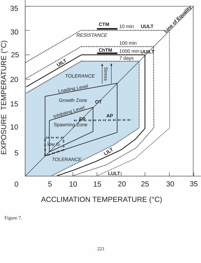
Figure 7.

5 10 15 20 25 30 35

5

10

15

20

25

30

35

0

ACCLIMATION TEMPERATURE (°C)

EX

PO

SU

RE

TE

MP

ER

AT

UR

E (

°C)

7 days1000 min

100 min

10 min UULT

LULT

LILT

UUILT

UILT

FP

Line o

f Equ

ality

OT

CTM

ChTM

TOLERANCE

RESISTANCE

TOLERANCE

Inhibiting Level

Loading Level

Growth Zone

Spawning Zone

low G

AP

Stress

221

Figure 8. The lower limit to distribution of spring chinook juveniles observed in the NorthFork John Day by Lindsay et al. (1986) in terms of mean maximum water temperature (°C).

222

0

20

40

60

80

100

Low

er D

istr

ibut

ion

Lim

it (R

iver

KM

)

8 12 16 20 24

Mean Max. Water Temp. at RK 71 (C)

Lower Limit of Chinook JuvenileDistribution--N.F. John Day River

Lower Spawning Limit

R =0.62Y= -26.8+4.31X p < 0.0012

Figure 8.

223

Figure 9. The maximum extent of distribution of spawning and rearing of spring chinook inthe John Day River, showing the mainstem John Day, North Fork John Day, Middle ForkJohn Day, and Upper Mainstem John Day as separate production units. Rearing area ismarked in dotted red; spawning are is marked in solid blue. Rearing can occur in spring tothe downstream extent indicated; below this point rearing is not feasible because of excessivetemperatures. Rearing, but not spawning, can also occur in certain headwater areas indicated. Based on information taken from Lindsay et al. (1986).

224

NORTH FORK JOHN DAY

MIDDLE FORK

Camas Cr.

Desolation Cr.

Camp Cr.

Spray

Kimberly

Prairie City

Dayville

Clarno

SO

UTH

FOR

K

Murderers Cr. Canyon Cr.

John Day

COLUMBIA RIVER

Granite Cr.

Clear Cr.

North Fork JDR

Oregon

John Day River Basin

N

30 600

KILOMETERS

Spawning (and rearing)

Rearing

Figure 9.

225

Figure 10. Times to 10, 50, and 90% mortality of chinook at test temperatures ranging from24°C to 29°C in 1°C increments based on a formula by Blahm and McConnell (1970) asreported in Coutant (1972).

226

1E-2

1E-1

1E0

1E1

1E2

1E3

Tim

e to

Dea

th (

hour

s)

0 20 40 60 80 100 Percent Mortality After 20C Acclim.

Times to Death at Test TemperaturesChinook (Blahm and McConnell 1970)

29

28

27

26

25

24

Figure 10.

227

Figure 11. Times to 50% mortality for juvenile spring chinook acclimated to either 20 or24°C. Data taken from Brett (1952).

228

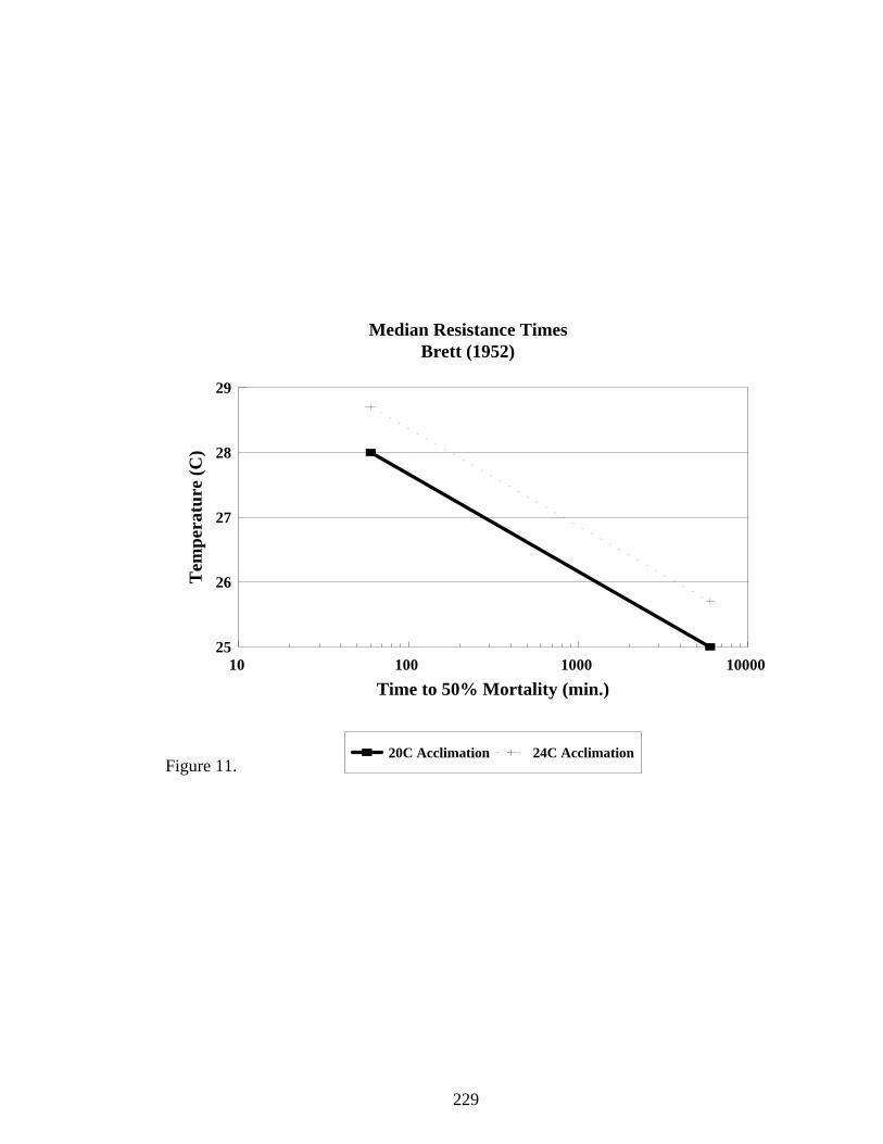
25

26

27

28

29

Tem

pera

ture

(C

)

10 100 1000 10000

Time to 50% Mortality (min.)

20C Acclimation 24C Acclimation

Median Resistance TimesBrett (1952)

Figure 11.

229

Figure 12. Tucannon River water temperatures (daily maximum, mean, and minimum) forAugust 1991 at the Marengo Bridge site (RK 41). The period of temperatures where themaximum daily temperature exceeded 23°C is highlighted.

230

16

18

20

22

24

26

28

0 5 10 15 20 25 30

Wat

er T

empe

ratu

re (

˚C)

August 1991

Maximum Minimum Mean

Tucannon River Temperaturesat Marengo Bridge (RK 41) for August 1991

Figure 12. 231

Figure 13. Tucannon River water temperatures (daily maximum, mean, and minimum) forAugust 1991 at the Deer Lake site (RK 62) as reported in Bugert et al. (1992).

232

1 2 3 4 5 6 7 8 9 10 11 12 13 14 15 16 17 18 19 20 21 22 23 24 25 26 27 28 29 30 31

12

14

16

18

20

22

24

26

Tem

per

atu

re (

C)

August 1991

Daily Max. Daily Mean Daily Min.

Figure 13.

233

Figure 14. Tucannon River maximum daily water temperatures for the period July 1-September 30 at Cummings Creek for years 1986-1997. Data provided courtesy of JosephBumgarner, WDFW, Dayton, Washington.

234

5

7

9

11

13

15

17

19

21

23

25W

ater

Tem

pera

ture

(˚C

)

Date

1986

1987

1988

1989

1990

1991

1992

1993

1994

1995

1996

1997

Tucannon River at Cummings CreekJuly 1-September 30

August 1 September 1July 1

Figure 14.

235

Figure 15. Tucannon River maximum daily water temperatures for the period July 1-September 30 at Marengo Bridge for years 1989-1997. Data provided courtesy of JosephBumgarner, WDFW, Dayton, Washington.

236

Tucannon River at Marengo BridgeJuly 1-September 30

August 1 September 1

10

12

14

16

18

20

22

24

26

28

30

Wat

er T

empe

ratu

re (

˚C)

Date

1989

1990

1991

1992

1993

1994

1995

1996

1997

July 1

Figure 15. 237

Figure 16. The percentage of days in July/August 1991 reaching maximum daily watertemperatures at Marengo Bridge, Tucannon River.

238

20 to

21

21 to

22

22 to

23

23 to

24

24 to

25

25 to

26

26 to

27

27 to

28

0

5

10

15

20

25

30

Per

cent

age

of D

ays

Daily Maximum Temperature (C)

Percentage of Days in July/August Period (1991)Reaching Maximum Daily Water Temperatures at Marengo Bridge

Figure 16.

239

Figure 17. Tucannon River water temperatures (daily maximum, mean, and minimum; also7-d moving mean of the maximum daily temperature and 7-d moving mean of the meandaily temperature) for July-August 1991 at the Marengo Bridge site (RK 41).

240

16.0

18.0

20.0

22.0

24.0

26.0

28.0

0 10 20 30 40 50 60

Tem

pera

ture

(o C

)

Days from July 1

Max (C) Min (C) Mean (C) 7-d mean of max (C) 7-d mean of mean (C)

Tucannon River Temperatures at Marengo BridgeJuly-August, 1991

Figure 17.241

Figure 18. Tucannon River water temperatures (daily maximum, mean, and minimum; also7-d moving mean of the maximum daily temperature and 7-d moving mean of the meandaily temperature) for September 1-30, 1991 at the Marengo Bridge site (RK 41).

242

10.0

12.0

14.0

16.0

18.0

20.0

22.0

24.0

0 5 10 15 20 25 30

Tem

pera

ture

(o C

)

September 1-30

Tucannon River Temperatures at Marengo BridgeSeptember, 1991

Max Min Mean 7-d Meanof Means

7-d Meanof Max

Figure 18. 243

Figure 19. Tucannon River water temperatures (daily maximum, mean, and minimum; also7-d moving mean of the maximum daily temperature and 7-d moving mean of the meandaily temperature) for September 1-30, 1991 at the Cummings Creek site.

244

10

12

14

16

18

20

22

0 5 10 15 20 25 30

Tem

pera

ture

(o C

)

September

Tucannon River Water TemperaturesMainstem near Cummings Creek, 1991

Max Min Mean

7-d Meanof Means

7-d Meanof Max

Figure 19. 245

Figure 20. Tucannon River average mean daily water temperatures for July estimated by useof stream segment temperature modeling (Theurer et al. 1985) for management alternativesranging from the current condition to restored mainstem conditions (restoration of riparianvegetation and channel morphology).

246

0

5

10

15

20

25

0 10 20 30 40 50 60 70 80 90 100

Wat

er T

empe

ratu

re (

˚C)

River Kilometer (Distance from mouth)

Restored

CurrentCondition

Tucannon River Water TemperaturesProfile of Average Mean Daily Temperature (July)

After Theurer et al. (1985)

Figure 20. 247

Figure 21. Maximum daily air temperature at LaGrande, Oregon and maximum daily watertemperature for the Tucannon River at Cummings Creek for August of 1988 and 1992.

248

10

15

20

25

30

35

40

0 5 10 15 20 25 30 35

Tem

pera

ture

(˚C

)

August

1988 (air) 1992 (air) 1988 (water) 1992 (water)

Maximum Daily Air Temperature (LaGrande, OR) and Maximum Daily WaterTemperature (Tucannon River at Cummings Cr.) for 1988 and 1992

Figure 21.249

Figure 22. Tucannon River (at Cummings Creek site) maximum daily water temperatures andthe ratio of maximum daily air temperature to mean daily stream discharge for the periodJuly-September, 1989. Air temperatures were taken from LaGrande, Oregon climatic stationwhich is 125 km air distance from Cummings Creek.

250

0

5

10

15

20

25

0

0.05

0.1

0.15

0.2

0.25

0.3

0.35

0.4

0.45

0 10 20 30 40 50 60 70 80 90 100

Max

imum

Dai

ly W

ater

Tem

pera

ture

(C

)

Max

. Dai

ly A

ir T

empe

ratu

re/M

ean

Dai

ly D

isch

arge

July-September Period1989 T(air)/Q

Tucannon River at Cummings Creek (Discharge, Water Temperature),Air Temperature at LaGrande, OR

Max. Daily Water Temperature

Figure 22. 251

LITERATURE CITED

Adams, B.L., W.S. Zaugg, and L.R. McLain. 1973. Temperature effect on parr-smolt transformation insteelhead trout (Salmo gairdneri) as measured by gill sodium-potassium stimulated adenosine triphosphatase. Comp. Biochem. Physiol. 44A:1333-1339.

Adams, B.L., W.S. Zaugg, and L.R. McLain. 1975. Inhibition of salt water survival and Na-K-ATPaseelevation in steelhead trout (Salmo gairdneri) by moderate water temperatures. Trans. Am. Fish. Soc. 104(4):766-769.

Alabaster, J.S. 1988. The dissolved oxygen requirements of upstream migrant chinook salmon, Oncorhynchustshawytscha, in the lower Willamette River, Oregon. J. Fish Biology 32:635-636.

Alabaster, J.S. 1989. The dissolved oxygen and temperature requirements of king salmon, Oncorhynchustshawytscha, in the San Joaquin delta, California. J. Fish Biol. 34(2):331-332.

Alabaster, J.S.and R. Lloyd. 1982. Water quality criteria for freshwater fish. 2nd edition. Food and AgricultureOrganization of the United Nations. Butterworths, London. 361 p.

Alcorn, S.R. 1976. Temperature tolerances and upper lethal limits of Salmo apache. Trans. Am. Fish. Soc.105(2):294-295.

Alderdice, D.F. and F.P.J. Velsen. 1978. Relation between temperature and incubation time for eggs of chinooksalmon (Oncorhynchus tshawytscha). J. Fish Res. Board Can. 35(1):69-75.

Andrew, F.J., and G.H. Geen. 1960. Sockeye and pink salmon production in relation to proposed dams in theFraser River system. Int. Pac. Salmon Fish. Comm. Bull. XI: 259 p.

Armour, C.L. 1990. Guidance for evaluating and recommending temperature regimes to protect fish. U.S. Fishand Wildlife Service. Fort Collins. Biological Report 90(22). 13 p.

Averett, R.C. 1969. Influence of temperature on energy and material utilization by juvenile coho salmon. Ph.D. Thesis, Oregon State Univ., Corvallis, Oregon. 74 p.

Bailey, J.E. and D.R. Evans. 1971. The low-temperature threshold for pink salmon eggs in relation to aproposed hydroelectric installation. Fish. Bull. 69:587-593.

Baker, P.F., T.P. Speed, and F.K. Ligon. 1995. Estimating the influence of temperature on the survival ofchinook salmon smolts (Oncorhynchus tshawytscha) migrating through the Sacramento-San Joaquin River Deltaof California. Can. J. Fish. Aquat. Sci. 52:855-863.

Barans, C.A. and R.A. Tubb. 1973. Temperatures selected seasonally by four fishes from western Lake Erie. J.Fish. Res. Board Can. 30:1697-1703.

Bartholow, J.M. 1989. Stream temperature investigations: field and analytic methods. Instream flow informationpaper no. 13. Biological Report 89(17). U.S. Fish and Wildlife Service. Fort Collins, Co. library> 4512McMurray Avenue, Fort Collins, CO 80525-3400

252

Bartholow, J.M. 1991. A modeling assessment of the thermal regime for an urban sport fishery. EnvironmentalManagement 15(6):833-845.

Barton, D.R., W.D. Taylor, and R.M. Biette. 1985. Dimensions of riparian buffer strips required to maintain trouthabitat in southern Ontario streams. N. Am. J. Fish. Manage. 5:364-378.

Beacham, T.D. 1988. A genetic analysis of early development in pink (Oncorhynchus gorbuscha) and chumsalmon (O. keta) at three different temperatures. Genome 30:89-96.

Beacham, T.D. and C.B. Murray. 1985. Effect of female size, egg size, and water temperature on developmentalbiology of chum salmon (Oncorhynchus keta) from the Nitinat River, British Columbia. Can. J. Fish. AquaticSci. 42(11):1755-1765.

Beacham, T.D. and C.B. Murray. 1986. Comparative developmental biology of chum salmon (Oncorhynchuskisutch) from the Fraser River, British Columbia. Can. J. Fish. Aquat. Sci. 43:252-262.

Beacham, T.D. and C.B. Murray. 1989. Variation in developmental biology of sockeye salmon (Oncorhynchusnerka) and chinook salmon (Oncorhynchus tshawytscha) in British Columbia. Can. J. Zool. 67:2081-2089.

Beacham, T.D. and C.B. Murray. 1990. Temperature, egg size, and development of embryos and alevins of fivespecies of Pacific salmon: a comparative analysis. Trans. Am. Fish. Soc 119(6):927-945.

Beacham, T.D. and T.P.T. Evelyn. 1992. Genetic variation in disease resistance and growth of chinook, coho,and chum salmon with respect to vibriosis, furunculosis, and bacterial kidney disease. Trans. Am. Fish. Soc.121:456-485.

Beacham, T.D. and R.E. Withler. 1991. Genetic variation in mortality of chinook salmon, Oncorhynchustshawytscha (Walbaum), challenged with high water temperatures. Aquacult. Fish. Manage. 22(2):125-133.

Beacham, T.D., R.E. Withler, C.B. Murray, and L.W. Barner. 1988. Variation in body size, morphology, eggsize, and biochemical genetics of pink salmon in British Columbia. Trans. Am. Fisheries Society 117(2):109-126.

Beamish, F.W.H. 1978. Swimming capacity. p. 101-187. In: Fish Physiology. Volume VII. Academic Press, Inc.

Becker, C.D. 1973. Columbia River thermal effects study: reactor effluent problems. Water Pollution ControlFederation 45(5):850-869.

Becker, C.D. and R.G. Genoway. 1979. Evaluation of the critical thermal maximum for determining thermaltolerance of freshwater fish. Environmental Biology of Fishes 4(3):245-256.

Becker, C.D. and M.G. Wolford. 1980. Thermal resistance of juvenile salmonids sublethally exposed to nickeldetermined by the critical thermal maximum method. Environmental Protection 21:181-189.

Becker, C.D., R.G. Genoway, and M.J. Schneider. 1977. Comparative cold resistance of three Columbia Riverorganisms. Trans. Am. Fish. Soc. 106(2):178-184.

Behnke, R.J. 1992. Native trout of western North America. American Fisheries Society Monograph 6. AmericanFisheries Society. Bethesda, Maryland. 275 p.

Bell, M.C. 1986. Fisheries handbook of engineering requirements and biological criteria. US Army Corps of

253

Engineers. Fish Passage Development and Evaluation Program, North Pacific Division, Portland, Oregon.

Bell, M.C. 1991. Fisheries handbook of engineering requirements and biological criteria. US Army Corps ofEngineers. Fish Passage Development and Evaluation Program, North Pacific Division, Portland, Oregon.

Bennett, D.H., M.H. Karr, and M.A. Madsen. 1997. Thermal and velocity characteristics in the Lower SnakeRiver reservoirs, Washington, as a result of regulated upstream water releases. U.S. Army Corps of Engineersfinal completion report. Project 14-16-0009-1579. 178 p.

Bennett, W.A., R.W. McCauley, and T.L. Beitinger. 1998. Rates of gain and loss of heat tolerance in channelcatfish. Trans. Am. Fish. Soc. 127:1051-1058.

Berman, C.H. 1990. The effect of elevated holding temperatures on adult spring chinook salmon reproductivesuccess. M.S. thesis. University of Washington. Seattle, WA.

Berman, C.H. and T.P. Quinn. 1990. The effect of elevated holding temperatures on adult spring chinooksalmon reproductive success. Submitted to TFW Cooperative Monitoring, Evaluation, and Research Committee,Center for Streamside Studies, Fisheries Research Institute, Seattle, Washington.

Berman, C.H. and T.P. Quinn. 1991. Behavioral thermoregulation and homing by spring chinook salmon,Oncorhynchus tshawytscha (Walbaum), in the Yakima River. J. Fish Biology 39:301-312.

Beschta, R.L., R.E. Bilby, G.W. Brown, L.B. Holtby, and T.D. Hofstra. 1987. Stream temperature and aquatichabitat: fisheries and forestry interactions. p. 191-231. In: E.O. Salo and T.W. Cundy, editors. Streamsidemangement: forestry and fishery interactions. College of Forest Resources, University of Washington, Seattle.Contribution No. 57. Proceedings of a Symposium held at University of Washington, February 12-14, 1986.

Bidgood, B.F. and A.H. Berst. 1969. Lethal temperatures for Great Lakes rainbow trout. J. Fisheries Res. BoardCan. 26:456-459.

Biesinger, K.E., R.P. Brown, C.R. Bernick, G.A. Flittner, and K.E.F. Hokanson. 1979. A national compendiumof freshwater fish and water temperature data. Volume I: Data management techniques, output examples andlimitations. EPA/600/3-79/056.

Biette, R.M. and G.H. Geen. 1980. Growth of underyearling sockeye salmon (Oncorhynchus nerka) underconstant and cyclic temperatures in relation to live zooplankton ration size. Can. J. Fish. Aquatic Sci. 37(2):203-210.

Bilby, R.E. 1984. Characteristics and frequency of cool-water areas in a western Washington stream. J.Freshwater Ecol. 2(6):593-602.

Billard, R. 1985. Environmental factors in salmonid culture and the control of reproduction. p. 70-87. In: R.N.Iwamoto and S. Sower (eds.). Salmonid reproduction: an international symposium. Washington Sea GrantProgram, Seattle, Washington.

Bilton, H.T. and H.D. Smith. 1973. Relationship between egg size and fish size in pink salmon (Oncorhynchusgorbuscha) from the lower Babine River in 1966 and 1967. Fish. Res. Board Can. Manuscr. Rep. No. 1235.

Binns, N.A. and F.E. Eiserman. 1979. Quantification of fluvial trout habitat in Wyoming. Trans. Am. Fish. Soc.108(3):215-228.

254

Biro, P.A. 1998. Staying cool: behavioral thermoregulation during summer by young-of-year brook trout in alake. Trans. Am. Fish. Soc. 127:212-222.

Bishai, H.M. 1960. Upper lethal temperatures for larval salmonids. J. Cons. Cons. Perm. Intern Explor. Mer25:129-133.

Bisson, P.A. and G.E. Davis. 1976. Production of juvenile chinook salmon, Oncorhynchus tshawytscha, in aheated model stream. NOAA Fish. Bull. 74(4):763-774.

Bisson, P.A., J.L. Nielson, and J.W. Ward. 1988. Summer production of coho salmon stocked in Mount St.Helens streams 3-6 years after the 1980 eruption. Trans. Am. Fish. Soc. 117:322-335.

Bjornn, T.C. and J. Mallet. 1964. Movements of planted and wild trout in an Idaho river system. Trans. Am.Fish. Soc. 93:70-76.

Bjornn, T.C. and D.W. Reiser. 1991. Habitat requirements of anadromous salmonids. Influences of forest andrangeland management on salmonid fishes and their habitats. Am. Fish. Soc. Special Publ. 19: 83-138.

Black, E.C. 1953. Upper lethal temperatures of some British Columbia fishes. J. Fish. Res. Board Can. 10:196-200.

Black, M.C., D.S. Millsap, and J.F. McCarthy. 1991. Effects of acute temperature change on respiration andtoxicant uptake by rainbow trout, Salmo gairdneri (Richardson). Physiol. Zool. 64(1):145-168.

Bouck, G.R., G.A. Chapman, P.W. Schneider, and D.G. Stevens. 1975. Effects of holding temperatures onreproductive development in adult sockeye salmon (Oncorhynchus nerka). p. 24-40. In: J.R. Donaldson (ed.)26th annual Northwest Fish Culture Conference, Otter Creek, Oregon.

Bowlby, J.N. and J.C. Roff. 1986. Trout biomass and habitat relationships in southern Ontario streams. Trans.Am. Fish. Soc. 115:503-514.

Brett, J.R. 1946. Rate of gain of heat tolerance in goldfish (Carassius auratus). Univ. Toronto Stud., Biol. Ser.No. 53, Publ. Ont. Fish Res. Lab. No. 64:9-28.

Brett, J.R. 1952. Temperature tolerance in young Pacific salmon, genus Oncorhynchus. J. Fish. Res. Bd. Can.9(6):265-323.

Brett, J.R. 1956. Some principles of the thermal requirements of fishes. Quarterly Review of Biology31(2):75-87.

Brett, J.R. 1958. Implications and assessments of environmental stress. p. 69-83. In: P.A. Larkin (ed).Investigations of fish-power problems. H.R. MacMillan Lectures in Fisheries, Univ. of British Columbia.

Brett, J.R. 1971. Energetic responses of salmon to temperature. A study of some thermal relations in thephysiology and freshwater ecology of sockeye salmon (Oncorhynchus nerka). Am. Zool. 11(1):99-113.

Brett, J.R. 1983. Life energetics of sockeye salmon, Oncorhynchus nerka. p. 29-63. In: W.P. Aspey and S.I.Lustick (eds.). Behavioral energetics: the cost of survival in vertebrates. Ohio State University Press.

Brett, J.R. and N.R. Glass. 1973. Metabolic rates and critical swimming speeds of sockeye salmon(Oncorhynchus nerka). J. Fish. Res. Bd. Can. 30:379-387.

255

Brett, J.R. and J.E. Shelbourn. 1975. Growth rate of young sockeye salmon, Oncorhynchus nerka, in relation tofish size and ration level. J. Fish. Res. Board Can. 32:2103-3110.

Brett, J.R., W.C. Clarke, and J.E. Shelbourn. 1982. Experiments on thermal requirements for growth and foodconversion efficiency of juvenile chinook salmon, Oncorhynchus tshawytscha. Can. Tech. Rep. Fish. Aquat. Sci.1127. 29 p.

Brett, J.R., M. Hollands, and D.F. Alderdice. 1958. The effect of temperature on the cruising speed of youngsockeye and coho salmon. J. Fish. Res. Board Can. 15(4):587-605.

Brett, J.R., J.E. Shelbourn, and C.T. Shoop. 1969. Growth rate and body composition of fingerling sockeyesalmon, Oncorhynchus nerka, in relation to temperature and ration size. J. Fish. Res. Bd. Can. 26(9):2363-2394.

Brown, L.R. 1989. Temperature preferences and oxygen consumption of three species of sculpin (Cottus) fromthe Pit River drainage, California. Environmental Biology of Fishes 26:223-226.

Brungs, W.A. and B.R. Jones. 1977. Temperature criteria for freshwater fish: protocol and procedures. EPA-600-3-77-061. Environmental Research Laboratory-Duluth, Office of Research and Development, US EnvironmentalProtection Agency. 136 p.

Bugert, R., C. Busack, G. Mendel, L. Ross, K. Petersen, D. Marbach, and J. Dedloff. 1991. Lower Snake RiverCompensation Plan. Tucannon River spring chinook salmon hatchery evaluation program. 1990 Annual report.Washington Department of Fisheries. Olympia, WA. AFF 1/LSR-91-14. 81 p.

Bugert, R., K. Petersen, G. Mendel, L. Ross, D. Milks, J. Dedloff, and M. Alexandersdottir. 1992. Lower SnakeRiver Compensation Plan. Tucannon River spring chinook salmon hatchery evaluation program. 1991 Annualreport. Washington Department of Fisheries. Olympia, WA. AFF 1/LSR-92-08. 91 p.

Bumgarner, J., G. Mendel, D. Milks, L. Ross, and J. Dedloff. 1995. Tucannon River spring chinook salmonhatchery evaluation program. 1994 Annual report. Washington Department of Fish and Wildlife, Olympia,Washington. Report H95-05 to US Fish and Wildlife Service, Cooperative Agreement 14-48-001-94544.

Bumgarner, J., G. Mendel, D. Milks, L. Ross, and J. Dedloff. 1996. Tucannon River spring chinook salmonhatchery evaluation. 1995 Annual report. Washington Department of Fish and Wildlife, Olympia, Washington.Report H96-07 to US Fish and Wildlife Service, Cooperative Agreement 14-48-0001-95572.

Bumgarner, J., G. Mendel, D. Milks, L. Ross, M. Varney, and J. Dedloff. 1997. Tucannon River springchinook hatchery evaluation. 1996 Annual report. Washington Department of Fish and Wildlife HatcheriesProgram Assessment and Development Division. Report #H97-07. Produced for US Fish and Wildlife Service,Cooperative Agreement 14-48-0001-96539.

Burck, W.A. 1994. Life history of spring chinook salmon in Lookingglass Creek, Oregon. Information Reports,Number 94-1. Oregon Department of Fish and Wildlife, Fish Division. 148 p.

Burck, W.A., R.B. Lindsay, B.J. Smith, and E.A. Olsen. 1980. Spring chinook studies in the John Day River.Federal Aid Progress Reports, Fisheries, Fish Research Project, Contract Number DEAC79-80BP18234. OregonDepartment of Fish and Wildlife. 69 p.

Burger, C.V., R.L. Wilmot, and D.B. Wangaard. 1985. Comparison of spawning areas and times for two runs ofchinook salmon (Oncorhynchus tshawytscha) in the Kenai River, Alaska. Can. J. Fish. Aquat. Sci. 42:693-700.

256

Burrows, R. 1963. Water temperature requirements for maximum productivity of salmon. p. 29-38. In: Watertemperature influences, effects, and control. Proc. 12th Northwest Symp. Water Pollution Research. U.S.Department of Health, Education, and Welfare, Public Health Service, Pacific Northwest Water Laboratory,Corvallis, Oregon.

Burton, G.W. and E.P. Odum. 1945. The distribution of stream fish in the vicinity of Mountain Lake, Virginia.Ecology 26:182-194.

Cada, G.F., J.M. Loar, and M.J. Sale. 1987. Evidence of food limitation of rainbow and brown trout insouthern Appalachian soft-water streams. Trans. Am. Fish. Soc. 116:692-702.

California Department of Water Resources (CDWR). 1988. Water temperature effects on chinook salmon(Oncorhynchus tshawytscha) with emphasis on the Sacramento River: a literature review. Northern District OfficeReport, Red Bluff, California. 42 p.

Calow, P. 1985. Adaptive aspects of energy allocation. p. 13-31. In: P. Tytler and P. Calow (ed.). Fishenergetics. Johns Hopkins University Press, Baltimore, Maryland.

Cech, J.J., Jr., S.J. Mitchell, D.T. Castleberry, and M. McEnroe. 1990. Distribution of California stream fishes:influence of environmental temperature and hypoxia. Env. Biol. Fishes 29:95-105.

Charlon, N., B. Barbier, and L. Bonnet. 1970. Résistance de la truite arc-en-ciel (Salmo gairdneri Richardson) ades variations brusques de température. Ann. Hydrobiol. 1(1):73-89.

Chen, Y.D. and H. Chen. 1993. Determining stream temperature changes caused by harvest of riparianvegetation: an overview. p. 313-323. In: Proceedings of the conference on riparian ecosystems in the humid U.S.:functions, values and management, Atlanta, GA, March 15-18, 1993.

Cherry, D.S., K.L. Dickson, and J. Cairns, Jr. 1975. Temperatures selected and avoided by fish at variousacclimation temperatures. J. Fish. Res. Board Can. 32(4):485-491.

Cherry, D.S., K.L. Dickson, J. Cairns Jr., and J.R. Stauffer. 1977. Preferred, avoided, and lethal temperatures offish during rising temperature conditions. J. Fish. Res. Board Can. 34:239-246.

Christie, G.C. and H.A. Regier. 1988. Measures of optimal thermal habitat and their relationship to yields forfour commercial fish species. Can. J. Fish. Aquat. Sci. 45:301-314.

Claire, E.W. and B.J. Smith. 1990. John Day fish district. Unpublished status report on wild spring chinook,wild summer steelhead, resident trout, smallmouth bass and channel catfish, bull trout, and cutthroat trout.Portland, Oregon.

Clapp, D.F., R.D. Clark, Jr., and J.S. Diana. 1990. Range, activity, and habitat of large, free-ranging browntrout in a Michigan stream. Trans. Am. Fish. Soc. 119:1022-1034.

Clarke, W.C. 1978. Growth of underyearling sockeye salmon (Oncorhynchus nerka) on diel temperature cycles.Fish . Environ. Can. Fish. Mar. Serv. Tech. Rep. 780. 19 p. fluctuating

Clarke, W.C. and J.E. Shelbourn. 1977. Effect of temperature photoperiod and salinity on growth and smoltingof underyearling coho salmon. Am. Zool. 17:957. Clarke, W.C. and J.E. Shelbourn. 1985. Growth and development of seawater adaptability by juvenile fall

257

chinook salmon (Oncorhynchus tshawytscha) in relation to temperature. Aquaculture 45:21-31.

Clarke, W.C., J.E. Shelbourn, and J.R. Brett. 1981. Effect of artificial photoperiod cycles, temperature, andsalinity on growth and smolting in underyearling coho (Oncorhynchus kisutch), chinook (O. tshawytscha), andsockeye (O. nerka) salmon. Aquaculture 22:105-116.

Cleland, B. 1997. Clean Water Act Section 303(d)/Water quality limited streams and temperature. Presentationgiven at the Columbia/Snake River mainstem water temperature workshop. Integrated ecosystem management ofthe Columbia River basin. November 6-7, 1997. Portland State University, Portland, OR.

Colgrove, D.J. and J.W. Wood. 1966. Occurrence and control of Chondrococcus columnaris as related to FraserRiver sockeye salmon. Progress report no. 15. International Pacific Salmon Fisheries Commission, BritishColumbia, Canada. 51 p.

Colwell, R.K. 1974. Predictability, constancy, and contingency of periodic phenomena. Ecology 55:1148-1153.

Combs, B.D. 1965. Effect of temperature on the development of salmon eggs. Prog. Fish-Cult. 27(3):134-137.

Combs, B.D. and R.E. Burrows. 1957. Threshold temperatures for the normal development of chinook salmoneggs. Prog. Fish Cult. 19:3-6.

Coutant, C.C. 1970. Thermal resistance of adult coho (Oncorhynchus kisutch) and jack chinook (O. tshawytscha)salmon, and adult steelhead trout (Salmo gairdneri) from the Columbia River. Battelle Memorial Inst., Pac.Northwest Lab., Richland, WA. Rep. No. BNWL-1508, UC-48. 24 p.

Coutant, C.C. 1972. Water quality criteria. A report of the committee on water quality criteria. p. 151-170 (text)and Appendix II-C (p. 410-419). In: National Academy of Sciences, National Academy of Engineers, EPA Ecol.Res. Series EPA-R3-73-033, US Environmental Protection Agency, Washington, D.C. 594 p.

Coutant, C.C. 1973. Effect of thermal shock on vulnerability of juvenile salmonids to predation. J. Fish. Res.Board Can. 30(7):965-973.

Coutant, C.C. 1977. Compilation of temperature preference data. J. Fish. Res. Board Can. 34:739-745.

Coutant, C.C. 1987. Thermal preference: when does an asset become a liability? Environmental Biology ofFishes 18(3):161-172.

Craigie, D.E. 1963. An effect of water hardness in the thermal resistance of the rainbow trout, Salmo gairdneriRichardson. Can. J. Zoology 41:825-831.

Craik, J.C.A. 1985. Egg quality and egg pigment content in salmonid fishes. Aquaculture 47:61-88.

Crisp, D.T. 1981. A desk study of the relationship between temperature and hatching time for the eggs of fivespecies of salmonid fishes. Freshwater Biology 11:361-368.

Crisp, D.T. 1990. Water temperature in a stream gravel bed and implications for salmonid incubation. FreshwaterBiology 23:601-612.

Crisp, D.T. and G. Howson. 1982. Effect of air temperature upon mean water temperature in streams in the northPennines and English Lake District. Freshwater Biol. 12:359-367.

258

CRITFC. 1995. Wy-Kan-Ush-Mi Wa-Kish-Wit, Spirit of the Salmon. The Columbia River anadromous fishrestoration plan of the Nez Perce, Umatilla, Warm Springs and Yakama Tribes. Volume I. Columbia River Inter-Tribal Fish Commission. Portland, OR.

Crone, R.A. and C.E. Bond. 1976. Life history of coho salmon, Oncorhynchus kisutch, in Sashin Creek,southeastern Alaska. National Marine Fisheries Service Fishery Bulletin 74:897-923.

Cunjak, R.A. and J.M. Green. 1986. Influence of water temperature on behavioural interactions between juvenilebrook charr, Salvelinus fontinalis, and rainbow trout, Salmo gairdneri. Can. J. Zool. 64(6):1288-1291.

Dahlberg, M.L., D.L. Shumway, and P. Doudoroff. 1968. Influence of dissolved oxygen and carbon dioxide onswimming performance of largemouth bass and coho salmon. J. Fish. Res. Board Can. 25:49-70.

Danzmann, R.G. and M.M. Ferguson. 1988a. Developmental rates of heterozygous and homozygous rainbowtrout reared at three temperatures. Biochem. Genet. 26(1/2):53-67.

Danzmann, R.G. and M.M. Ferguson. 1988b. Temperature-dependent genotypic selection and embryonic survivalof rainbow trout. Biochem. Genet. 26(1/2):69-81.

Dauble, D.D. and D.G. Watson. 1997. Status of fall chinook salmon populations in the mid-Columbia River,1948-1992. N. Am. J. Fisheries Management 17:283-300.

Daykin, P.N. 1965. Application of mass transfer theory to the problem of respiration of fish eggs. J. Fish. Res.Board Can. 22:159-171.

de Gaudemar, B. and E. Beall. 1998. Effects of overripening on spawning behaviour and reproductive successof Atlantic salmon females spawning in a controlled flow channel. J. Fish. Biol. 53:434-446.

DeHart, D.A. 1975. Resistance of three freshwater fishes to fluctuating thermal environments. M.S. Thesis.Oregon State University, Corvallis, Oregon.

DeLacy, A.C., S.P. Felton, and G.J. Paulik. 1956. A study to investigate the effects of fatigue and currentvelocities on adult salmon and steelhead trout. p. 126-138. In: Prog. Rep. on Fish. Eng. Res. Prog., N. Pac. Div.,US Army Corps Eng., Portland, OR.

DeVries, P. 1997. Riverine salmonid egg burial depths: review of published data and implications for scourstudies. Can. J. Fish. Aquat. Sci. 54:1685-1698.

Dickson, I.W. and R.H. Kramer. 1971. Factors influencing scope for activity and active standard metabolism ofrainbow trout (Salmo gairdneri). J. Fish. Res. board Can. 28:587-596.

Dimick, R.E. and F. Merryfield. 1945. The fishes of the Willamette River system in relation to pollution. OregonState College Engineering Experiment Station Bulletin Series 20:7-55. Oregon State College, Corvallis, Oregon.

Dingman, S.L. 1972. Equilibrium temperatures of water surfaces as related to air temperature and solar radiation.Wat. Resour. Res. 8:42-49.

Dockray, J.J., S.D. Reid, and C.M. Wood. 1996. Effects of elevated summer temperatures and reduced pH onmetabolism and growth of juvenile rainbow trout (Oncorhynchus mykiss) on unlimited ration. Can. J. Fish.Aquat. Sci. 53:2752-2763.

259

Donaldson, L.R. and F.J. Foster. 1941. Experimental study of the effect of various water temperatures on thegrowth, food utilization, and mortality rate, of fingerling sockeye salmon. Trans. Am. Fish. Soc. 70:339-346.

Dwyer, W.P. and R.H. Kramer. 1975. The influence of temperature on scope for activity in cutthroat trout,Salmo clarki. Trans. Am. Fish. Soc. 104:522-554.

Eaton, J.G., J.H. McCormick, B.E. Goodno, D.G. O'Brien, H.G. Stefany, M. Hondzo, and R.M. Scheller. 1995.A field information-based system for estimating fish temperature tolerances. Fisheries 20(4):10-18.

Edwards, R.W., J.W. Densen, and P.A. Russell. 1979. An assessment of the importance of temperature as afactor controlling the growth rate of brown trout in streams. J. Anim. Ecol. 48:501-507.

Elliott, J.M. 1975a. The growth rate of brown trout (Salmo trutta L.) fed on maximum rations. J. AnimalEcology 44:805-821.

Elliott, J.M. 1975b. The growth rate of brown trout, Salmo trutta L., fed on reduced rations. J. Animal Ecology44:823-842.

Elliott, J.M. 1981. Some aspects of thermal stress on freshwater teleosts. p. 209-245. In: Stress and fish. A.D.Pickering (ed.). Academic Press.

Elliott, J.M. 1994. Quantitative ecology and the brown trout. Oxford Series in Ecology and Evolution, Serieseditors R.M. May and P.H. Harvey. Oxford University Press, Oxford, England. 286 p.

Elliott, J.M. and J.A. Elliott. 1995. The effect of the rate of temperature increase on the critical thermalmaximum for parr of Atlantic salmon and brown trout. J. Fish Biol. 47:917-919.

Environmental Protection Agency and National Marine Fisheries Service (EPA and NMFS). 1971. ColumbiaRiver Thermal Effects Study. Volume 1. Biological Effects Study. U.S. Environmental Protection Agency andNational Marine Fisheries Service. 102 p.

Erman, D.C. and G.R. Leidy. 1975. Downstream movement of rainbow trout fry in a tributary of Sagehen Creek,under permanent and intermittent flow. Trans. Am. Fish. Soc. 104:467-473.

Espinosa, F.A., Jr., J.J. Rhodes, and D.A. McCullough. 1997. The failure of existing plans to protect salmonhabitat on the Clearwater National Forest in Idaho. J. Env. Management 49(2):205-230.

Evans, D.O. 1990. Metabolic thermal compensation by rainbow trout: effects on standard metabolic rate andpotential usable power. Trans. Am. Fish. Soc. 119:585-600.

Ewing, R.D., S.L. Johnson, H.J. Pribble, and J.A. Lichatowich. 1979. Temperature and photoperiod effects ongill (Na+K)-ATPase activity in chinook salmon (Oncorhynchus tshawytscha). J. Fish. Res. Board Can. 36:1347-1353.

Fausch, K.D. 1989. Do gradient and temperature affect distributions of, and interactions between, brook charr(Salvelinus fontinalis) and other resident salmonids in streams? Physiology and Ecology Japan, Special Volume1:303-322.

Fausch, K.D. and R.J. White. 1981. Competition between brook trout (Salvelinus fontinalis) and brown trout(Salmo trutta) for positions in a Michigan stream. Can. J. Fish. Aq. Sciences 38:1220-1227.

260

Fausch, K.D. and M.K. Young. 1995. Evolutionarily significant units and movement of resident stream fishes: acautionary tale. American Fisheries Society Symposium 17:360-370.

Fedorov, K.Ye. and L.S. Bogdanova. 1978. The growth and development of the larvae of the pink salmon,Oncorhynchus gorbuscha, under different temperature and feeding regimes. J. Ichthyol. 18(4):568-576.

Feldmeth, C.R. and C.H. Eriksen. 1978. A hypothesis to explain the distribution of native trout in a drainage ofMontana's Big Hole River. Internationale Vereinigung fur theroetische und angewandte LimnologieVerhandlungen 20:2040-2044.

FEMAT. 1993. Forest ecosystem management: an ecological, economic, and social assissment. USFS, NMFS,USBLM, USFWS, USNPS, and USEPA. US Forest Service PNW Region, Portland, Oregon.

Ferguson, H.W. 1981. The effects of water temperature on the development of proliferative kidney disease inrainbow trout, Salmo gairdneri Richardson. J. Fish Dis. 4(2):175-177.

Ferguson, R.G. 1958. The preferred temperatures of fish and their midsummer distribution in temperate lakes andstreams. J. Fish. Res. Board Can. 15:607-624.

Fields, R., S.S. Lowe, C. Kaminski, G.S. Whitt, and D.P. Philipp. 1987. Critical and chronic thermal maxima ofnorthern and Florida largemouth bass and their reciprocal F1 and F2 hybrids. Trans. Am. Fish. Soc. 116:856-863.

Fish, F.F. 1944. The retention of adult salmon with particular reference to the Grand Coulee Fish SalvageProgram. U.S. Fish and Wildlife Service Special Scientific Report No. 27.

Fish, F.F. 1948. The return of blueback salmon to the Columbia River. Scientific Monthly (Wash), 66:283-292.

Fish, F.F. and M.G. Hanavan. 1948. A report upon the Grand Coulee fish-maintenance project 1939-1947. U.S.Fish and Wildlife Service, Special Science Report 55. 63 p.

Fish, F.R. and R.R. Rucker. 1943. Columnaris as a disease of freshwater fishes. Trans. Am. Fisheries Society73:32-36.

Flett, P.A., K.R. Munkittrick, G. Van Der Kraak, and J.F. Leatherland. 1996. Overripening as the cause of lowsurvival to hatch in Lake Erie coho salmon (Oncorhynchus kisutch) embryos. Can. J. Zool. 74:851-857.

Folmar, L.C., W.W. Dickhoff, C.V.W. Mahnken, and F.W. Waknitz. 1982. Stunting and parr-reversion duringsmoltification of coho salmon (Oncorhynchus kisutch). Aquaculture 28:91-104.

Frissell, C.A., R.K. Nawa, and W.J. Liss. 1992. Water temperature and distribution and diversity of salmonidfishes in Sixes River Basin, Oregon, USA: changes since 1965-1972. p. 127-172. In: C.A. Frissell. 1992.Cumulative effects of land use on salmon habitat in southwest Oregon coastal streams. Ph.D. thesis, Oregon StateUniversity, Corvallis, Oregon.

Frost, W.E. and M.E. Brown. 1967. The trout. New Naturalist Series, Collins, St. James Place. London.

Fry, F.E.J. 1947. Effects of the environment on animal activity. Univ. Toronto Stud., Biol. Ser., No. 55. Pub.Ont. Fish. Res. Lab., No. 68. 62 p.

Fry, F.E.J. 1957. The lethal temperature as a tool in taxonomy. Ann. Biol. 33:205-219.

261

Fry, F.E.J. 1971. The effect of environmental factors on the physiology of fish. p. 1-98. In: W.S. Hoar and D.J.Randall (ed.). Fish physiology. Vol. VI: Environmental relations and behavior. Academic Press, Inc. San Diego,CA.

Fry, F.E.J. and M.B. Gibson. 1953. Lethal temperature experiments with speckled trout x lake trout hybrids. J.Hered. 44(2):56-57.

Fry, F.E.J., J.S. Hart, and N.F. Walker. 1946. Lethal temperature relations for a sample of young speckled trout,Salvelinus fontinalis. Univ. Toronto Studies, Biol. Ser. 54, Ontario Fish. Res. Lab. Publ. 66:9-35.

Fryer, J.L. and K.S. Pilcher. 1974. Effects of temperature on diseases of salmonid fishes. US EnvironmentalProtection Agency. Office of Research and Development, Ecological Research Series EPA-660/3-73-020. 114 p.

Fryer, J.L., K.S. Pilcher, J.E. Sanders, J. Rohovec, J.L. Zinn, W.J. Groberg, and R.H. McCoy. 1976.Temperature, infectious diseases, and the immune response in salmonid fish. U.S. Environ. Prot. Agency Ecol.Res. Ser. EPA-600/3-76-21. 70 p.

Fujihara, M.P. and F.P. Hungate. 1970. Seasonal distribution of Chondrococcus columnaris disease in riverfishes: a procedure using antibody synthesis in fishes as a survey technique. Battelle Northwest, BNWL-SA-3563. SH 177 .C49 F854 1970.

Fujihara, M.P. and R.E. Nakatani. 1970. Antibody production and immune response of rainbow trout and cohosalmon to Chondrococcus columnaris. October 1, 1970. Manuscript 43 prepared for Columbia River ThermalEffects Study by NMFS.

Fujihara, M.P., P.A. Olson, and R.E. Nakatani. 1971. Some factors in susceptibility of juvenile rainbow trout andchinook salmon to Chondrococcus columnaris. J. Fish. Res. Bd. Can. 28:1739-1743.

Gard, R. and G.A. Flittner. 1974. Distribution and abundance of fishes in Sagehen Creek, California. J. WildlifeManagement 38:347-358.

Garling, D.L. and M. Masterson. 1985. Survival of Lake Michigan chinook salmon egs and fry incubated at threetemperatures. Prog. Fish-Culturist 47:63-66.

Garside, E.T. and J.S. Tait. 1958. Preferred temperature of rainbow trout (Salmo gairdneri, Richardson) and itsunusual relationship to acclimation temperature. Can. J. Zool. 36:563-567.

Gibson, R.J. 1966. Some factors influencing the distributions of brook trout and young Atlantic salmon. J. Fish.Res. Board Can. 23:1977-1980.

Gilhousen, P. 1980. Energy sources and expenditures in Fraser River sockeye salmon during their spawningmigration. Int. Pac. Salmon Fish. Comm. Bull. XXII: 51p.

Gilhousen, P. 1990. Prespawning mortalities of sockeye salmon in the Fraser River system and possible causalfactors. Bull. Int. Pac. Salmon Fisheries Comm. 26: 62 p.

Goddard, C.I. and J.S. Tait. 1976. Preferred temperatures of F3 to F5 hybrids of Salvelinus fontinalis x S.namaycush. J. Fish. Res. Board Can. 33:197-202.

Godin, J-G. J. 1981. Migrations of salmonid fishes during early life history phases: daily and annual timing. p.22-50. In: E.L. Brannon and E.O. Salo (ed.). Proceedings of the salmon and trout migratory behavior

262

symposium. School of Fisheries, Univ. of Washington, Seattle, WA.

Golden, J.T. 1975. Immediate effects of logging on the freshwater environment salmonids: lethal temperatures forcoastal cutthroat trout under fluctuating temperature regimes: job progress report, 1974-1975. Oregon Dept. FishWildlf. Fed. Aid Prog. Rep. Anadrom. Fish Proj. AFS-585: 7 p.

Golden, J.T. 1976. Lethal temperatures for coastal cutthroat trout under fluctuating temperature regimes. FederalAid Progress Reports, Fisheries. Oregon Department of Fish and Wildlife. 14 p.

Golden, J.T. and C.B. Schreck. 1978. Effects of fluctuating temperatures on the thermal tolerance limits ofcoastal cutthroat trout Salmo clarki clarki). Unpublished m.s., Oregon Department of Fish and Wildlife.Corvallis, Oregon.

Grabowski, S.J. 1973. Effects of fluctuating and constant temperatures on some hematological characteristics,tissue glycogen levels, and growth of steelhead trout (Salmo gairdneri). Ph.D. dissertation, University of Idaho.77 p.

Grande, M. and S. Andersen. 1991. Critical thermal maxima for young salmonids. J. Freshwater Ecology6(3):275-279.

Graynoth, E. 1979. Effects of logging on stream environments and faunas in Nelson.New Zealand Journal Marine and Freshwater Research 13(1):79-109.

Gresswell, R.E. 1995. Yellowstone cutthroat trout. p. 36-54. In: M.K. Young (tech. ed.). Conservation assessmentfor inland cutthroat trout. USDA Forest Service, Gen. Tech. Report RM-GTR-256.

Griffiths, J.S. and D.F. Alderdice. 1972. Effects of acclimation and acute temperature experience on theswimming speed of juvenile coho salmon. J. Fish. Res. Board Can. 29(3):251-264.

Groberg, W.J., Jr., R.H. McCoy, K.S. Pilcher, and J.L. Fryer. 1978. Relation of water temperature to infectionsof coho salmon (Oncorhynchus kisutch), chinook salmon (O. tshawytscha), and steelhead trout (Salmo gairdneri)with Aeromonas salmonicida and A. hydrophila. J. Fish. Res. Board Can. 35(1):1-7.

Groberg, W.J., Jr., J.S. Rohovec, and J.L. Fryer. 1983. The effects of water temperature on infection andantibody formation induced by Vibrio anguillarum in juvenile coho salmon (Oncorhynchus kisutch). J. WorldMaricult. Soc. 14:240-248.

Hahn, P.K.J. 1977. Effects of fluctuating and constant temperatures on behavior of steelhead trout (Salmogairdneri). Ph.D. dissertation, University of Idaho. 142 p. Dissertation Abstracts Int. B Sci. Eng. 38(12):5668.

Hall, L.W., Jr., C.H. Hocutt, and J.R. Stauffer, Jr. 1978. Implication of geographic location on temperaturepreference of white perch, Morone americana. J. Fish. Res. Board Can. 35:1464-1468.

Hallock, R.J., R.F. Elwell, and D.H. Fry. 1970. Migrations of adult kind salmon Oncorhynchus tshawytscha inthe San Joaquin Delta as demonstrated by the use of sonic tags. California Dept. Fish Game Fish Bull. 151. 92 p.

Hart, J.S. 1947. Lethal temperature relations of certain fish of the Toronto region. Trans. Roy. Soc. Can. Sec.5(41):57-71.

Hart, J.S. 1952. Geographic variations of some physiological and morphological characters in certain freshwater

263

fish. University of Toronto biology series no. 60. The University of Toronto Press, Toronto. 79 p.

Hartman, G.F., L.B. Holtby, and J.C. Scrivener. 1984. Some effects of natural and logging-related winter streamtemperature changes on the early life history of the coho salmon (Oncorhynchus kisutch) in Carnation Creek,British Columbia. p. 141-149. In: W.R. Meehan, T.R. Merrell, Jr., and T.A. Hanley (eds.). Fish and wildliferelationships in old-growth forests; proceedings of a symposium. American Institute of Fishery ResearchBiologists, Morehead City, North Carolina.

Hartwell, S.I. and D.E. Hoss. 1979. Thermal shock resistance of spot (Leistomus xanthurus) after acclimation toconstant or cycling temperature. Trans. Am. Fisheries Soc. 108:397-400.

Hatch, D., A. Wand, A. Porter, and M. Schwartzberg. 1993. The feasibility of estimating sockeye salmonescapement at Zosel Dam using underwater video technology. 1992 Annual progress report prepared for PublicUtility District No. 1 of Douglas County. Columbia River Inter-Tribal Fish Commission, Portland, OR. 27 p.

Hawkins, C.P., M.L. Murphy, N.H. Anderson, and M.A. Wilzbach. 1983. Density of fish and salamanders inrelation to riparian canopy and physical habitat in streams of the northwestern United States. Canadian Journal ofFisheries and Aquatic Sciences 40:1173-1185.

Healey, M.C. 1991. Life history of chinook salmon (Oncorhynchus tshawytscha). p. 311-393. In: C. Groot and L.Margolis (ed.). Pacific salmon life histories. UBC Press, Vancouver. 564 p.

Healey, T. 1979. The effect of high temperature on the survival of Sacramento River chinook (king) salmon,Oncorhynchus tshawytscha), eggs and fry. California Department of Fish and Game, Anadromous FisheriesBranch, Administrative Report No. 79-10. 7 p.

Heath, W.G. 1963. Thermoperiodism in the sea-run cutthroat (Salmo clarki clarki). Science 142:486-488.

Hedrick, R.P., M.L. Kent, R. Rosemark, and D. Manzer. 1984. Proliferative kidney disease (PKD) in Pacificsalmon and steelhead trout. J. World Maricul. Soc. 15:318-325.

Heming, T.A. 1982. Effecs of temperature on utilization of yolk by chinook salmon (Oncorhynchustshawytscha) eggs and alevins. Can. J. Fish. Aquat. Sci. 39:184-190.

Henjum, M.G., J.R. Karr, D.L. Bottom, D.A. Perry, J.C. Bednarz, S.G. Wright, S.A. Beckwitt. 1994. Interimprotection for late successional forests, fisheries, and watersheds: national forests east of the Cascade Crest,Oregon and Washington. The Wildlife Society, Bethesda, MD.

Hetrick, F.M., J.L. Fryer, and M.D. Knittel. 1979. Effect of water temperature on the infection of rainbow troutSalmo gairdneri Richardson with infectious hematopoietic necrosis virus. J. Fish. Dis. 2(3):253-257.

Hoar, W.S. 1988. The physiology of smolting salmonids. In: W.S. Hoar and D.J. Randall (eds.). Fish physiology.Vol XIB. p. 275-343. Academic Press, New York, NY.

Hoffmaster, J.L., J.E. Sanders, J.S. Rohovec, J.L. Fryer, and D.G. Stevens. 1988. Geographic distribution of themyxosporean parasite, Ceratomyxa shasta Noble, 1950, in the Columbia River basin, USA. J. Fish Diseases11(1):97-100.

Hokanson, K.E.F. 1977. Temperature requirements of some percids and adaptations to seasonal temperaturecycle. J. Fisheries Research Board of Can. 34(10):1524-1550.

264

Hokanson, K.E.F., C.F. Kleiner, and T.W. Thorslund. 1977. Effects of constant temperatures and diel temperaturefluctuations on specific growth and mortality rates and yield of juvenile rainbow trout, Salmo gairdneri. J. Fish.Res. Board Can. 34(5):639-648.

Hokanson, K.E.F., J.H. McCormick, B.R. Jones, and J.H. Tucker. 1973. Thermal requirements for maturation,spawning, and embryo survival of the brook trout (Salvelinus fontinalis). J. Fish. Res. Board Can. 30:975-984.

Holt, R.A., J.E. Sanders, J.L. Zinn, J.L. Fryer, and K.S. Pilcher. 1975. Relation of water temperature toFlexibacter columnaris infection in steelhead trout (Salmo gairdneri), coho (Oncorhynchus kisutch) and chinook(O. tshawytscha) salmon. J. Res. Fish. Board Can. 32(9):1553-1559.

Holtby, B.L. 1988. Effects of logging on stream temperatures in Carnation Creek, British Columbia, andassociated impacts on the coho salmon (Oncorhynchus kisutch). Canadian Journal of Fisheries and AquaticScience 45:502-515.

Holtby, L.B., T.E. McMahon, and J.C. Scrivener. 1989. Stream temperatures and inter-annual variability in theemigration timing of coho salmon (Oncorhynchus kisutch) smolts and fry and chum salmon (O. keta) fry fromCarnation Creek, British Columbia. Can. J. Fish. Aquat. Sci. 46:1396-1405.

Holtby, L.B. and J.C. Scrivener. 1989. Observed and simulated effects of climatic variability, clear-cut loggingand fishing on the numbers of chum salmon (Oncorhynchus keta) and coho salmon (Oncorhynchus kisutch)returning to Carnation Creek, British Columbia. p. 62-81. In: C.D. Levings, L.B. Holtby, and M.A. Henderson(eds.). Proceedings of the national workshop on effects of habitat alterations on salmonid stocks. CanadianSpecial Publication of Fisheries and Aquatic Sciences 105, Ottawa, Ontario, Canada.

Horning, W.B. and R.E. Pearson. 1973. Growth temperature requirements and lower lethal temperatures forjuvenile small bass (Micropterus dolomieui). J. Fish. Res. Board Can. 30:1226-1230.

Hostetler, S.W. 1991. Analysis and modeling of long-term stream temperatures on the Steamboat Creek Basin,Oregon: implications for land use and fish habitat. Water Resources Bull. 27(4):637-647.

Hubert, W.A. and W.A. Gern. 1995. Influence of embryonic stage on survival of cutthroat trout exposed totemperature reduction. Prog. Fish-Culturist 57:326-328.

Hubert, W.A., R.W. Stonecypher, Jr., Gern, W.A., and J. Bobbit. 1994. Response of cutthroat trout embryos toreduced incubation temperatures at different developmental stages. Prog. Fish-Culturist 56:185-187.

Humpesch, U.H. 1985. Inter- and intra-specific variation in hatching success and embryonic development of fivespecies of salmonids and Thymallus thymallus. Arch. Hydrobiol. 104(1):129-144.

Hutchison, V.H. and J.D. Maness. 1979. The role of behavior in temperature acclimation and tolerance inectotherms. Am. Zool. 19:367-384.

Idler, D.R. and W.A. Clemens. 1959. The energy expenditures of Fraser River sockeye salmon during thespawning migration to Chilko and Stuart Lakes. Prog. Rep., Int. Pac. Salmon Fish. Comm. 80 p.

Inskip, P.D. and J.J. Magnuson. 1983. Changes in fish populations over an 80-year period: Big Pine Lake,Wisconsin. Trans. Am. Fish. Soc. 112:378-389.

Iron, J.G., III, S.R. Ray, L.K. Miller, and M.W. Oswood. 1989. Spatial and seasonal patterns of streambed watertemperatures in an Alaskan subarctic stream. p. 381-390. In: Headwaters Hydrology. American Water Resources

265

Association.

Jensen, A.J. 1990. Growth of young migratory brown trout Salmo trutta correlated with water temperature inNorwegian rivers. J. Anim. Ecol. 59(2):603-614.

Jensen, A.J., B.O. Johsen, and L. Saksgard. 1989. Temperature requirements in Atlantic salmon (Salmo salar),brown trout (Salmo trutta), and Arctic char (Salvelinus alpinus) from hatching to intitial feeding compared withgeographic distribution. Can. J. Fish. Aquat. Sci. 46:786-789.

Jobling, M. 1981. Temperature tolerance and final preferendum-rapid methods for the assessment of optimumgrowth temperatures. J. Fish Biology 19:439-455.

Jobling, M. 1993. Bioenergetics: feed intake and energy partitiioning. p. 1-43. In: J.C. Rankin and F.B. Jensen(ed.). Fish ecophysiology. Chapman and Hall. London.

Johnson, J. 1960. Sonic tracking of adult salmon at Bonneville Dam, 1957. U.S. Fish. Wildl. Serv., Fish. Bull.176:471-485.

Johnson, H.E. and R.F. Brice. 1953. Effects of transportation of green eggs, and of water temperature duringincubation, on the mortality of chinook salmon. Prog. Fish-Culturist 15:104-108.

Johnston, C.E. and R.L. Saunders. 1981. Parr-smolt transformation of yearling Atlantic salmon (Salmo salar) atseveral rearing temperatures. Can. J. Fish. Aquat. Sci. 38(10):1189-1198.

Jowett, J.G. 1990. Factors related to the distribution and abundance of brown and abundance of brown andrainbow trout in New Zealand clear-water rivers. N.Z. J. Mar. Freshwat. Res. 24(3):429-440.

Karr, M.H., J.K. Fryer, and P.R. Mundy. 1998. Snake River water temperature control project. Phase II.Methods for managing and monitoring water temperatures in relation to salmon in the lower Snake River. Columbia River Inter-Tribal Fish Commission, Prepared for U.S. Environmental Protection Agency, Region 10,Contract No. X-990375-01-1. 209 p.

Karr, M., B. Tanovan, R. Turner, and D. Bennett. 1992. Interim report: model studies and 1991 operations.Water temperature control project, Snake River. Columbia River Inter-Tribal Fish Commission, US Army Corpsof Engineers, and University of Idaho Fish and Wildlife Resources Department. 58 p.

Kaya, C.M. 1978. Thermal resistance of rainbow trout from a permanently heated stream, and of two hatcherystrains. Prog. Fish-Culturist 40(4):138-142.

Kaya, C.M., L.R. Kaeding, and D.E. Burkhalter. 1977. Use of a cold-water refuge by rainbow and brown trout ina geothermally heated stream. Prog. Fish-Culturist 39(1):37-39.

Keleher, C.J. and F.J. Rahel. 1996. Thermal limits to salmonid distributions in the Rocky Mountain Region andpotential habitat loss due to global warming: a geographic information system (GIS) approach. Trans. Am. Fish.Soc. 125(1):1-13.

Kellogg, R.L. and J.J. Gift. 1983. Relationship between optimum temperatures for growth and preferredtemperatures for the young of the four fish species. Trans. Am. Fish. Soc. 112:424-430.

Kelsch, S.W. 1996. Temperature selection and performance by bluegills: evidence for selection in response toavailable power. Trans. Am. Fish. Soc. 125:948-955.

266

Kelsch, S.W. and W.H. Neill. 1990. Temperature preference versus acclimation in fishes: selection for changingmetabolic optima. Trans. Am. Fish. Soc. 119:601-610.

Kilgour, D.M. and R.W. McCauley. 1986. Reconciling the two methods of measuring upper lethal temperaturesin fishes. Environmental Biology of Fishes 17(4):281-290.

King, W. 1937. Notes on the distribution of native speckled and rainbow trout in the streams at Great SmokyMountians National Park. J. Tenn. Acad. Sci. 12:351-361.

Konecki, J.T., C.A. Woody, and T.P. Quinn. 1993. Thermal adaptations of Washington coho salmon(Oncorhynchus kisutch)populations: incubation, preference and tolerance. School of Fisheries, Center forStreamside Studies, University of Washington WH-10, Seattle, WA. 34 p.

Konecki, J.T., C.A. Woody, and T.P. Quinn. 1995a. Critical thermal maxima of coho salmon (Oncorhynchuskisutch) fry under field and laboratory acclimation regimes. Can. J. Zool. 73:993-996.

Konecki, J.T., C.A. Woody, and T.P. Quinn. 1995b. Temperature preference in two populations of juvenilecoho salmon, Oncorhynchus kisutch. Env. Biol. Fishes 44:417-421.

Konstantinov, A.S., V.V. Zdanovich, and D.G. Tikhomirov. 1989. Effect of temperature oscillation on themetabolic rate and energetics of young fish. J. Ichthyology 29( 6):1019-1027.

Kovacs, T.G. and G. Leduc. 1982. Acute toxicity of cyanide to rainbow trout (Salmo gairdneri) acclimated atdifferent temperatures. Can. J. Fish. Aquat. Sci. 39:1426-1429.

Kwain, W. 1975. Effects of temperature on development and survival of rainbow trout, Salmo gairdneri, in acidwaters. J. Fish. Res. Board Can. 32(4):493-497.

Kwain, W. and R.W. McCauley. 1978. Effects of age and overhead illumination on temperatures preferred byunderyearling rainbow trout, Salmo gairdneri, in a vertical temperature gradient. J. Fish. Res. Board Can.35(11):1430-1433.

Lattenmaier, D.P. and T.Y. Gan.1990. Hydrologic sensitivities of the Sacramento-San-Joaquin River Basin,California, to global warming. Water Resources Res. 26(1):69-86.

Lee, R.M. and J.N. Rinne. 1980. Critical thermal maxima of five trout species in the southwestern United States.Trans. Am. Fish. Soc. 109(6):632-635.

Leitritz, E. and R.C. Lewis. 1976. Trout and salmon culture. California Department of Fish and Game. FishBulletin 164. 197 p.

Li, H.W., G.A. Lamberti, T.N. Pearsons, C.K. Tait, J.L. Li, and J.C. Buckhouse. 1994. Cumulative effects ofriparian disturbances along high desert trout streams of the John Day Basin, Oregon. Trans. Am. Fish. Soc.123:627-640.

Li, H.W., T.N. Pearsons, C.K. Tait, J.L. Li, and R. Gaither. 1992. Approaches to evaluate habitat improvementprograms in streams of the John Day Basin. Oregon Cooperative Fishery Research Unit, Department of Fisheriesand Wildlife, Oregon State University. Completion Report.

Li, H.W., C.B. Schreck, C.E. Bond, and E. Rexstad. 1987. Factors influencing changes in fish assemblages ofPacific Northwest streams. p. 193-202. In: Matthews, W.J. and D.C. Heins (eds.). Community and evolutionary

267

ecology of North American stream fishes. Univ. of Oklahoma Press. Norman and London.

Lindsay, R.B., B.C. Jonasson, R.K. Schroeder, and B.C. Cates. 1989. Spring chinook salmon in the DeschutesRiver, Oregon. Information Reports, No. 89-4. Oregon Department of Fish and Wildlife. 92 p.

Lindsay, R.B., W.J. Knox, M.W. Flesher, B.J. Smith, E.A. Olsen, and L.S. Lutz. 1986. Study of wild springchinook salmon in the John Day River system. 1985 Final Report. Oregon Department of Fish and Wildlife.Bonneville Power Administration, Division of Fish and Wildlife, Contract No. DE-A179-83BP39796, Project No.79-4.

Lohr, S.C., P.A. Byorth, C.M. Kaya, and W.P. Dwyer. 1996. High-temperature tolerances of fluvial Arcticgrayling and comparisons with summer river temperatures of the Big Hole River, Montana. Trans. Am. Fish.Soc. 125:933-939.

Lyons, J., and L. Wang, T.D. Simonson. 1996. Development and validation of an index of biotic integrity forcoldwater streams in Wisconsin. N. Am. J. Fisheries Management 16(2):241-256.

Mabbott, L.B. 1982. Density and habitat of wild and introduced juvenile steelhead trout in the Lochsa Riverdrainage, Idaho. Master's thesis. University of Idaho, Moscow.

Madison, D.M., R.M. Horrall, A.B. Stasko, and A.D. Hasler. 1972. Migrating movements of adult sockeyesalmon (Oncorhynchus nerka) in coastal British Columbia as revealed by ultrasonic tracking. J. Fish. Res. BoardCan. 29:1025-1033.

Magnuson, J.J., L.B. Crowder, and P.A. Medvick. 1979. Temperature as an ecological resource. Amer. Zool19:331-343.

Mahnken, C.V.W. and F.W. Waknitz. 1979. Factors affecting growth and survival of coho salmon(Oncorhynchus kisutch) and chinook salmon (O. tshawytscha) in saltwater net-pens in Puget Sound. Proc. WorldMaricul. Soc. 10:280-305.

Major, R.L. and J.L. Mighell. 1967. Influence of Rocky Reach Dam and the temperature of the Okanogan Riveron the upstream migration of sockeye salmon. Fishery Bull. 66(1):131-147.

Mantelman, I.I. 1960. Distribution of the young of certain species of fish in temperature gradients. FisheriesBoard of Canada Translation Series 257.

Margolis, L. and T.P.T. Evelyn. 1975. Ceratomyxa shasta (Myxosporida) disease in chum salmon (Oncorhynchusketa) in British Columbia. J. Fish. Res. Board Can. 32:1640-1643.

Margolis, L., T.E. McDonald, and D.J. Whitaker. 1992. Assessment of the impact of the myxosporean parasiteCeratomyxa shasta on survival of seaward migrating juvenile chinook salmon, Oncorhynchus tshawytscha, fromthe Fraser River, British Columbia. Can. J. Fish. Aquat. Sci. 49:1883-1889.

Marine, K.R. 1992. A background investigation and review of the effects of elevated water temperature onreproductive performance of adult chinook salmon (Oncorhynchus tshawytscha) with suggestions for approachesto the assessment of temperature induced reproductive impairment of chinook salmon stocks in the AmericanRiver, California. Unpublished manuscript, prepared for the American River Technical Advisory Committee.Department of Wildlife and Fisheries Biology, University of California, Davis, California.

Marine, K.R. and J.J. Cech, Jr. 1998. Effects of elevated water temperatuare on some aspects of the

268

physiological and ecological performance of juvenile chinook salmon (Oncorhynchus tshawytscha): implicationsfor management of California's chinook salmon stocks. Stream temperature monitoring and assessmentworkshop. January 12-14, 1998. Sacramento, California. Forest Science Project, Humboldt State University,Arcata, California.

Marr, D.H.A. 1966. Influence of temperatuare on the efficiency of growth of salmonid embryos. Nature(Lond.)212(5065):957-959.

Marten, P.S. 1992. Effect of temperature variation on the incubation and development of brook trout eggs. TheProgressive Fish-Culturist 54:1-6.

Martin, D.J., L.J. Wasserman, and V.H. Dale. 1986. Influence of riparian vegetation on posteruption survival ofcoho salmon fingerlings on the west-side streams of Mount St. Helens, Washington. N. Am. J. FisheriesManagement 6(1):1-8.

Mather, D. and C.A. Silver. 1980. Statistical problems in studies of temperature preference of fishes. Can. J.Fish. Aquat. Sci. 37:733-737.

Mathur, D., R.M. Schutsky, E.J. Purdy, Jr., and C.A. Silver. 1981. Similarities in acute temperature preferencesof freshwater fishes. Trans. Am. Fish. Soc. 110:1-13.

Mattax, B.L. and T.M. Quigley. 1989. Validation and sensitivity analysis of the stream network temperaturemodel on small watersheds in northeast Oregon. p. 391-400. In: Woessner, W.W. and D.F. Potts (eds.). Am.Water Resour. Ass., Proc. of the Symp. on Headwaters Hydrology.

Matthews, K.R. and N.H. Berg. 1997. Rainbow trout responses to water temperature and dissolved oxygenstress in two southern California stream pools. J. Fish Biology 50:50-67.

McCauley, R.W. 1958. Thermal relations of geographic races of Salvelinus. Can. J. Zool. 36(5):655-662.

McCauley, R.W. and W.L. Pond. 1971. Temperature selection of rainbow trout (Salmo gairdneri) fingerlings invertical and horizontal gradients. J. Fish. Res. Board Can. 28:1801-1804.

McCauley, R.W., J.R. Elliot, and A.L.A. Read. 1977. Influence of acclimation temperature on preferredtemperature in the rainbow trout, Salmo gairdneri. Trans. Am. Fish. Soc. 106:362-365.

McCormick, J.H. and J.A. Wegner. 1981. Responses of largemouth bass from different latitudes to elevated watertemperatures. Trans. Am. Fish. Soc. 110:417-429.

McCormick, J.H., K.E.F. Hokanson, and B.R. Jones. 1972. Effects of temperature on growth and survival ofyoung brook trout (Salvelinus fontinalis). J. Fish Res. Board Can. 29:1107-1112.

McCullough, D.A. 1975. Bioenergetics of three aquatic invertebrates determined by radioisotopic analyses. IdahoState University. 326 p.

McCullough, D.A. 1987. A systems classification of watersheds and streams. Ph.D. thesis. Oregon StateUniversity. 217 p.

McCullough, D.A. 1990. Classification of streams within a landscape perspective. 158 p. In: CoordinatedInformation System Project, Annual Progress Report, January 5, 1989- December 31, 1990. Prepared byColumbia River Inter-Tribal Fish Commission for Bonneville Power Commission.

269

McCullough, D.A. 1996. Stream carrying capacity and smolt production. p. 45-70. In: Proceedings from aworkshop on ecological carrying capacity of salmonids in the Columbia River Basin: Measure 7.1A of theNorthwest Power Planning Council's 1994 Fish and Wildlife Program. Report 3 of 4. Final report. USDepartment of Energy, Bonneville Power Administration. Project Number 93-012, Agreement Number DE-AI79-86BP62611.

McCullough, D.A. and F.A. Espinosa, Jr. 1996. A monitoring strategy for application to salmon-bearingwatersheds. Tech. Report 96-5. Columbia River Inter-Tribal Fish Commission, Portland, Oregon. 170 p. +appendices.

McCullough, D.A., G.W. Minshall, and C.E. Cushing. 1979. Bioenergetics of a stream "collector" organismTricorythodes minutus (Insecta: Ephemeroptera). Limnol. Oceanogr. 24(1):45-58.

McGeer, J.C., L. Baranyi, and G.K. Iwama. 1991. Physiological responses to challenge tests in six stocks of cohosalmon (Oncorhynchus kisutch). Can. J. Fish. Aquat. Sci. 48:1761-1771.

McIntosh, B.A., D.M. Price, C.E. Torgersen, and H.W. Li. 1995a. Distribution, habitat utilization, movementpatterns, and the use of thermal refugia by spring chinook in the Grande Ronde, Imnaha, and John Day Basins.Progress report to the Bonneville Power Administration, Project No. 88-108, FY-1995.

McIntosh, B.A., C.E. Torgersen, D.M. Price, and H.W. Li. 1995b. Distribution, habitat utilization, movementpatterns, and the use of thermal refugia by spring chinook in the Grande Ronde, Imnaha, and John Day Basins.Annual report to the Bonneville Power Administration, Project No. 93-7000, FY-1995.

McIntyre, J.D. and B.E. Rieman. 1995. Westslope cutthroat trout. p. 1-15. In: M.K. Young (tech. ed.).Conservation assessment for inland cutthroat trout. USDA Forest Service, Gen. Tech. Report RM-GTR-256.

McMahon, T.E. and G.F. Hartman. 1988. Variation in the degree of silvering of wild coho salmon,Oncorhynchus kisutch, smolts migrating seaward from Carnation Creek, British Columbia. J. Fish Biol. 32:825-833.

McMahon, T.E. and G.F. Hartman. 1989. Influence of cover complexity and current velocity on winter habitatuse by juvenile coho salmon (Oncorhynchus kisutch). Can. J. Fish. Aq. Sci. 46(9):1551-1557.

McRae, G. and C.J. Edwards. 1994. Thermal characteristics of Wisconsin headwater streams occupied by beaver:implications for brook trout habitat. Trans. Am. Fish. Soc. 123:641-656.

Meisner, J.D. 1990 . Potential loss of thermal habitat for brook trout, due to climatic warming, in two southernOntario streams. Trans. Am. Fish. Soc. 119:282-291.

Meisner, J.D., J.S. Rosenfeld, and H.A. Regier. 1988. The role of groundwater in the impact of climate warmingon stream salmonines. Fisheries 13(3):2-8.

Mesa, M.G., T.P. Poe, A.G. Maule, and C.B. Schreck. 1998. Vulnerability to predation and physiological stressresponses in juvenile chinook salmon (Oncorhynchus tshawytscha) experimentally infected with Renibacteriumsalmoninarum. Can. J. Fish. Aquat. Sci. 55:1599-1606.

Metcalfe, N.B. and J.E. Thorpe. 1992. Early predictors of life-history events: the link between first feeding date,dominance and seaward migration in Atlantic salmon, Salmo salar L. J. Fish Biol. 41(Suppl. B):93-99.

Moore, A.M. 1967. Correlation and analysis of water-termperature data for Oregon streams. U.S. Geological

270

Survey Water-Supply Paper 1819-K. 53 p.

Moyle, P.B. 1976. Inland fishes of California. University of California Press. Berkeley, California. 405 p.

Moyle, P.B. and D.M. Baltz. 1985. Microhabitat use by an assemblage of California stream fishes: developingcriteria for instream flow determinations. Trans. Am. Fish. Soc. 114:695-704.

Mullan, J.W., K.R. Williams, G. Rhodus, T.W. Hillman, and J.D. McIntyre. 1992. Production and habitat ofsalmonids in mid-Columbia River tributary streams. U.S. Fish and Wildlife Service, Monograph 1. 187 p. plusappendices.

Murphy, M.L. and J.D. Hall. 1981. Varied effects of clear-cut logging on predators and their habitat in smallstreams of the Cascade Mountains, Oregon. Canadian Journal of Fisheries and Aquatic Science 38:137-145.

Murray, C.B. 1980. Some effects of temperature on zygote and alevin survival, rate of development and size athatching and emergence of Pacific salmon and rainbow trout. M.S. thesis. University of British Columbia,Vancouver, B.C.

Murray, C.B. and T.D. Beacham. 1986. Effect of varying temperature regimes on the development of pinksalmon (Oncorhynchus gorbuscha) eggs and alevins. Can. J. Zool. 64:670-676.

Murray, C.B. and T.D. Beacham. 1987. The development of chinook (Oncorhynchus tshawytscha) and chumsalmon (Oncorhynchus keta) embryos and alevins under varying temperature regimes. Can. J. Zool. 65(11):2672-2681.

Murray, C.B., T.D. Beacham, and J.D. McPhail. 1990. Influence of parental stock and incubation temperature onthe early development of coho salmon (Oncorhynchus kisutch) in British Columbia. Can. J. Zool. 68:347-358.

Murray, C.B. and J.D. McPhail. 1988. Effect of incubation temperature on the development of five species ofPacific salmon (Oncorhynchus) embryos and alevins. Can. J. Zool. 66(1):266-273.

Murray, C.B., J.D. McPhail, and M.L. Rosenau. 1989. Reproductive and developmental biology of kokanee fromUpper Arrow Lake, British Columbia. Trans. Am. Fish. Soc. 118:503-509.

Nakamoto, R.J. 1994. Characteristics of pools used by adult summer steelhead oversummering in the NewRiver, California. Trans. Am. Fish. Soc. 123:757-765.

National Academy of Sciences (NAS). 1996. Upstream. Salmon and society in the Pacific Northwest.Committee on Protection and Management of Pacific Northwest Anadromous Salmonids. National AcademyPress.

National Academy of Sciences (NAS). 1972. Water quality criteria. Freshwater aquatic life and wildlife.Appendix II. EPA Ecol. Res. Series EPA-R3-73-033, US Environmental Protection Agency, Washington, D.C.594 p.

Neitzel, D.A., M.J. Scott, S.A. Shankle, and J.C. Chatters. 1991. The effect of climate change on streamenvironments: the salmonid resource of the Columbia River basin. Northwest Environmental Journal 7:271-293.

Newsome, G.E. and G. LeDuc. 1975. Seasonal changes of fat content in the yellow perch (Perca flavescens) oftwo Laurentian Lakes. J. Fish. Res. Board Can. 32:2214-2221.

271

Nielsen, J.L., T.E. Lisle, and V. Ozaki. 1994. Thermally stratified pools and their use by steelhead in northernCalifornia streams. Trans. Am. Fish. Soc. 123:613-626.

NMFS. 1998. Progress of species status reviews in NMFS Northwest Region. File 1pg898.pdf at NOAA websitehttp://www.nwr.noaa.gov.

Northwest Power Planning Council (NPPC). 1986. Council staff compilation of information on salmon andsteelhead losses in the Columbia River basin. NPPC, 850 S.W. Broadway, Suite 1100, Portland, Oregon 97205.252 p.

Norton, D.J., M.A. Flood, B.A. McIntosh, N.J. Poage, P.J. LaPlaca, J.P. Craig, R.S. Karalus, J.R. Sedell, C.E.Torgerson, Y.D. Chen, S.C. McCutcheon, V. Duong, H. Puffenberger, J. Moeller, V. Kelly, E. Porter, and L.Shoemaker. 1996. Modeling, monitoring and restoring water quality and habitat in Pacific Northwesternwatersheds. EPA GATF '95 Project. Abridged/unclassified version. April 1996.

Olsen, E., P. Pierce, M. McLean, and K. Hatch. 1993. Stock summary reports for Columbia River anadromoussalmonids. Vol. I: Oregon. Coordinated Information System. Prepared for U.S. Department of Energy, BonnevillePower Administration, Division of Fish and Wildlife, Contract No. 88-108. DOE/BP 94402-1 and 94402-2.

Olson, P.A. and R.F. Foster. 1955. Temperature tolerance of eggs and young of Columbia River chinook salmon.Trans. Am. Fish. Soc. 85:203-207.

Ordal, E.J. and R.E. Pacha. 1963. The effects of temperature on disease in fish. p. 39-56. Proc. Twelfth PacificNorthwest Symposium on water pollution research. Corvallis, Oregon.

Oregon Department of Environmental Quality (ODEQ). 1995. 1992-1994 Water quality standards review. Department of Environmental Quality, Standards and Assessment Section. Final issues papers. Portland,Oregon.

Pacha, R.E. 1961. Columnaris disease in fishes in the Columbia River Basin. Univ. of Washington, Ph.D.Thesis. 332 p.

Pacha, R.E. and E.J. Ordal. 1970. Myxobacterial diseases of salmonids. p. 243-257. In: S.F. Snieszko (ed.). Asymposium on diseases of fishes and shellfishes. Special Publication No. 5, American Fisheries Society,Washington, D.C.

Paladino, F.V., J.R. Spotila, J.P. Schubauer, and K.T. Kowalski. 1980. The critical thermal maximum: atechnique used to elucidate physiological stress and adaptation in fishes. Rev. Can. Biol. 39(2):115-122.

Parker, F.L. and P.A. Krenkel. 1969. Thermal pollution. Status of the art report. Report Number 3, Departmentof Environmental and Water Resources Engineering, Vanderbilt University, Nashville, Tennessee. Prepared forthe Federal Water Pollution Control Administration. Grant No. WP-01387-01.

Parrish, E.M. 1978. Evaluation of spring chinook salmon eigration, harvest and returns to Rapid River Hatchery,1977. Idaho Department of Fish and Game. Annual Performance Report, Project No. IPC-17 and IPC-13.

Paulik, G.J. 1960. The locomotive performance of salmonids during upstream migration. p. 41-42. In: T.S.Y.Koo (ed.). Research in fisheries...1959. Contrib. No. 77. Univ. Wash., College Fish., Seattle, WA.

Paulik, G.J. and A.C. DeLacy. 1958. Changes in the swimming ability of Columbia River sockeye salmonduring upstream migration. Univ. Wash., Sch. Fish., Tech. Rep. No. 46, p. 1-67.

272

Paulik, G.J., A.C. DeLacy, and E.F. Stacy. 1957. The effect of rest on the swimming performance of fatiguedadult silver salmon. Univ. Wash., Sch. Fish., Tech. Rep. No. 31, p. 1-24.

Peterson, R.H. and D.J. Martin-Robichaud. 1989. First feeding of Atlantic salmon (Salmo salar L.) fry asinfluenced by temperature regime. Aquaculture 78(1):35-53.

Peterson, R.H., H.C.E. Spinney, and A. Sreedharan. 1977. Development of Atlantic salmon (Salmo salar) eggsand alevins under varied temperature regimes. J. Fish. Res. Board Can. 34:31-43.

Peterson, R.H., A.M. Sutterlin, and J.L. Metcalfe. 1979. Temperature preference of several species of/ Salmo/and Salvelinus/ and some of their hybrids. J. Fish. Res. Board Can. 36(9):1137-1140.

Piper, R.G., I.B. McElwain, L.E. Orme, J.P. McCraren, L.G. Fowler, and J.R. Leonard. 1982. Fish hatcherymanagement. US Department of Interior. Fish and Wildlife Service. Washington, D.C. 517 p.

Platts, W.S. 1974. Geomorphic and aquatic conditions influencing salmonids and stream classification. SurfaceEnvironment and Mining Program. 199 p.

Poff, N.L. and J.V. Ward. 1989. Implications of streamflow variability and predictability for lotic communitystructure: a regional analysis of streamflow patterns. Can. J. Fish. Aq. Sci. 46:1805-1818.

Potter, I.C. and F.W.H. Beamish. 1975. Lethal temperatures in ammocoetes of four species of lampreys. ActaZoologica 56:85-91.

Power, M. and G. Power. 1994. Modeling the dynamics of smolt production in Atlantic salmon. Trans. Am. Fish.Soc. 123:535-548.

Pratt, K. 1984. Habitat use and species interaction of juvenile cutthroat trout (Salmo clarki lewisi) and bull trout(Salvelinus confluentus) in the upper Flathead River Basin. M.S. thesis, University of Idaho, Moscow, Idaho.

Preall, R.J. and N.H. Ringler. 1989. Comparison of actual and potential growth rates of brown trout (Salmotrutta) in natural streams based on bioenergetic models. Can. J. Fish. Aquat. Sci. 46:1067-1076.

Priede, I.G. 1985. Metabolic scope in fishes. p. 33-64. In: P. Tytler and P. Calow (eds.). Fish energetics newperspectives. The John Hopkins University Press, Baltimore, Maryland.

Quinn, T.P. and D.J. Adams. 1996. Environmental changes affecting the migratory timing of American shad andsockeye salmon. Ecology 77(4):1151-1162.

Quinn, T.P., S. Hodgson, and C. Peven. 1997. Temperature, flow, and the migration of adult sockeye salmon(Oncorhynchus kisutch) in the Columbia River. Can. J. Fish. Aquat. Sci. 54:1349-1360.

Rahel, F.J. and W.A. Hubert. 1991. Fish assemblages and habitat gradients in a Rocky Mountain-Great Plainsstream: biotic zonation and additive patterns of community change. Trans. Am. Fish. Soc. 120:319-332.

Raleigh, R.F., W.F. Miller, and P.C. Nelson. 1986. Habitat suitability index models and instream flow suitabilitycurves: chinook salmon. U.S. Fish Wildl. Service Biol. Rep. 82(10.122). 64 p.

Ratliff, D.E. 1981. Ceratomyxa shasta: epizootiology in chinook salmon of central Oregon. Trans. Am. FisheriesSoc. 110:507-513.

273

Ratliff, D.E. 1983. Ceratomyxa shasta: longevity, distribution, timing, and abundance of the infective stage incentral Oregon. Can. J. Fisheries and Aquatic Sciences 40:1622-1632.

Reeves, G.H., F.H. Everest, and J.D. Hall. 1987. Interaction between redside shiner (Richarsonius balteatus) andthe steelhead trout (Salmo gairdneri) in western Oregon: the influence of water temperature. Can. J. Fisheries andAquatic Sciences 44:1603-1613.

Reeves, G.H., J.D. Hall, and S.V. Gregory. 1997. The impact of land-management activities on coastal cutthroattrout and their freshwater habitats. p. 138-144. In: J.D. Hall, P.A. Bisson, and R.E. Gresswell (ed.). Sea-runcutthroat trout: biology, management, and future conservation. Oregon Chapter, American Fisheries Society,Corvallis.

Reiser, D.W. and T.C. Bjornn. 1979. Habitat requirements of anadromous salmonids. Gen. Tech. Rep. PNW-96.USDA Forest Service. Pacific Northwest Forest and Range Experiment Station. Portland, Oregon. 54 pp.

Reynolds, W.W. and M.E. Casterlin. 1979a. The role of temperature in the environmental physiology of fishes.In: M.A. Ali (ed.). Environmental physiology of fishes. Plenum Press, New York.

Reynolds, W.W. and M.E. Casterlin. 1979b. Behavioral thermal regulation and the 'final preferendum' paradigm.Amer. Zool 19:211-224.

Reynolds, W.W. and M.E. Casterlin. 1979c. Thermoregulatory behavior of brown trout, Salmo trutta. Hydrobiologia 62:79-80.

Rhodes, J.J., D.A. McCullough, and F.A. Espinosa, Jr. 1994. A coarse screening process for evaluation of theeffects of land management activities on salmon spawning and rearing habitat in ESA consultations. Tech. Report94-4. Columbia River Inter-Tribal Fish Commission, Portland, Oregon. 127 pp. + appendices.

Rice, G.V. 1960. Use of coldwater holding facilities in conjunction with king salmon spawning operations atNimbus Hatchery. Inland Fisheries Administrative Report Number 60-3.

Ricklefs, R.E. 1973. Ecology. Chiron Press, New York. 861 p.

Rodgers, D.W. and J.S. Griffiths. 1983. Effects of elevated thermal regimes on survival of rainbow trout (Salmogairdneri) alevins. J. Great Lakes Res. 9(3):421-424.

Ryder, R.A., W.B. Scott, and E.J. Crossman. 1964. Fishes of northern Ontario, north of the Albany River. R.Ont. Mus., Life. Sciences Contribution 60. 30 p.

Sadler, S.E., G.W. Friars, and P.E. Ihssen. 1986. The influence of temperature and genotype on the growth rateof hatchery-reared salmonids. Can. J. Anim. Sci. 66:599-606.

Sandercock, F.K. 1991. Life history of coho salmon (Oncorhynchus kisutch). p. 395-445. In: C. Groot and L.Margolis (ed.). Pacific salmon life histories. UBC Press, Vancouver. 564 p.

Sanders, J.E., K.S. Pilcher, and J.L. Fryer. 1978. Relation of water temperature to bacterial kidney disease incoho salmon (Oncorhynchus kisutch), sockeye salmon (O. nerka), and steelhead trout (Salmo gairdneri). J. Fish.Res. Board Can. 35(1):8-11.

Sauter, S.T. and A.G. Maule. 1997. The role of water temperature in the smolt physiology of chinook salmon.Presentation given at the Columbia/Snake River mainstem water temperature workshop. Integrated ecosystem

274

management of the Columbia River basin. November 6-7, 1997. Portland State University, Portland, OR.

Scarnecchia, D.L., A. Isaksson, and S.E. White. 1989. Oceanic and riverine influences on variations in yieldamong Icelandic stocks of Atlantic salmon. Trans. Am. Fish. Soc. 118:482-494.

Schreck, C.B., J.C. Snelling, R.E. Ewing, C.S. Bradford, L.E. Davis, and C.H. Slater. 1994. Migratory behaviorof adult spring chinook salmon in the Willamette River and its tributaries. Oregon Cooperative Fishery ResearchUnit, Oregon State University, Corvallis, Oregon. Project Number 88-160-3, Prepared for Bonneville PowerAdministration, Portland, Oregon.

Schurmann, H., J.F. Steffensen, and J.P. Lomholt. 1991. The influence of hypoxia on the preferred temperatureof rainbow trout Oncorhynchus mykiss. J. Exp. Biol. 157:75-86.

Scott, W.B. and E.J. Crossman. 1985. Freshwater fishes of Canada. Fisheries Research Board of Canada, Ottawa,1973. Bull. 184. The Bryant Press Limited. 966 p.

Servizi, J.A. and J.O.T. Jensen. 1977. Resistance of adult sockeye salmon to acute thermal shock. Progress reportno. 34. International Pacific Salmon Fisheries Commission, British Columbia, Canada. 51 p.

Servizi, J.A. and D.W. Martens. 1991. Effect of temperature, season, and fish size on acute lethality ofsuspended sediments to coho salmon (Oncorhynchus kisutch). Can. J. Fish. Aquat. Sci. 48:493-497.

Shepard, B.B., S.A. Leathe, T.M. Weaver, and M.D. Enk. 1984. Monitoring levels of fine sediment withintributaries to Flathead Lake and impacts of fine sediment on bull trout recruitment. Proceedings of the WildTrout III Symposium. Yellowstone Nat. Park, WY.

Shepherd, B.G., G.F. Hartman, and W.J. Wilson. 1986. Relationships between stream and intragraveltemperatures in coastal drainages, and some implications for fisheries workers. Can. J. Fisheries and AquaticSciences 43:1818-1822.

Slater, D.W. 1963. Winter-run chinook salmon in the Sacramento River, California with notes on watertemperature requirements at spawning. U.S. Fish and Wildlife Service, Special Scientific Report, Fisheries No.461. 9 p.

Smith, C.E., W.P. Dwyer, and R.G. Piper. 1983. Effect of water temperature on egg quality of cutthroat trout.Prog. Fish-Cult. 45(3):176-178.

Snake River Subbasin Plan. 1990. Snake River subbasin (Mainstem from mouth to Hells Canyon Dam). Salmonand steelhead production plan. September 1, 1990. Northwest Power Planning Council and Columbia Basin Fishand Wildlife Authority, Portland, Oregon.

Snieszko, S.F. 1964. Remarks on some facets of epizootiology of bacterial fish diseases. Devel. Indust.Microbiol. 5:97-100.

Snieszko, S.F. 1974. The effects of environmental stress on outbreaks of infectious diseases of fishes. J. Fish.Biol. 6:197-208.

Sonski, A.J. 1983a. Heat tolerance of redband trout. Annu. Proc. Tex. Chap. Am. Fish. Soc. 5:66-76.

Sonski, A.J. 1983b. Culture of redband trout at a warm-water hatchery. p. 21-40. Proceedings of Fish FarmingConference and Annual Convention of Catfish Farmers of Texas. Texas A&M University.

275

Sonski, A.J. 1984. Comparison of heat tolerances of redband trout, Firehole River rainbow trout, and Wythevillerainbow trout. Annu. Proc. Tex. Chap. Am. Fish. Soc. 6:27-35.

Spence, B.C., G.A. Lomnicky, R.M. Hughes, R.P. Novitzki. 1996. An ecosystem approach to salmonidconservation. TR-4501-96-6057. ManTech Environmental Research Services Corp., Corvallis, OR.

Spigarelli, S.A., M.M. Thommes, and W. Prepejchal. 1982. Feeding, growth, and fat deposition by brown trout inconstant and fluctuating temperatures. Trans. Am. Fish. Soc. 111(2):199-209.

Spigarelli, S.A., M.M. Thommes, W. Prepejchal, and R.M. Goldstein. 1983. Selected temperatures and thermalexperience of brown trout, Salmo trutta, in a steep thermal gradient in nature. Environ. Biol. Fishes.8(2):137-149.

Stabler, D.F. 1981. Effects of altered flow regimes, temperatures, and river impoundment on adult steelhead troutand chinook salmon. M.S. thesis, University of Idaho, Moscow, Idaho. 84 p.

Stauffer, J.R., Jr. 1980. Influence of temperature on fish behavior. p. 103-141. In: C.H. Hocutt, J.R. Stauffer, Jr.,J.E. Edinger, L.W. Hall, Jr., R.P. Morgan II. (eds.). 1980. Power plants. Effects on fish and shellfish behavior. Academic Press, New York.

Stauffer, J.R., J. Cairns, Jr., K.L. Dickson, and D.L. Cherry. 1976. The potential and realized influence oftemperature on the distribution of fishes in the New River, Glen Lyn, Va. Wildlife Monographs 50:1-40.6.

Stauffer, J.R., Jr., E.L. Melisky, and C.H. Hocutt. 1984. Interrelationships among preferred, avoided, and lethaltemperatures of three fish species. Arch. Hydrobiol. 100(2):159-169.

Stearns, S.C. 1981. On measuring fluctuating environments: predictability, constancy, and contingency. Ecology62:185-199.

Stefan, H.G. and E.B. Preud'homme. 1993. Stream temperature estimation from air temperature. Water Resour.Bull. 29:27-45.

Stonecypher, R.W., Jr., W.A. Hubert, and W.A. Gern. 1994. Effect of reduced incubation temperatures onsurvival of trout embryos. Prog. Fish-Culturist 56:180-184.

Stoneman, C.L. and M.L. Jones. 1996. A simple method to classify stream thermal stability with singleobservations of daily maximum water and air temperatures. N. Am. J. Fisheries Management 16:728-737.

Sullivan, K., J. Tooley, K. Doughty, J.E. Caldwell, and P. Knudsen. 1990. Evaluation of prediction models andcharacterization of stream temperature regimes in Washington. Timber/Fish/Wildlife Rep. No. TFW-WQ3-90-006. Washington Department of Natural Resources, Olympia, Washington. 224 p.

Sylvester, R.O. 1958. Water quality studies in the Columbia River Basin. U.S. Fish Wildlife Service Spec. Sci.Rep. Fish. No. 239. 134 p.

Tang, J., M.D. Bryant, and E.L. Brannon. 1987. Effect of temperature extremes on the mortality anddevelopment rates of coho salmon embryos and alevins. Prog. Fish-Cult. 49(3):167-174.

Taniguchi, R., F.J. Rahel, D.C. Novinger, and K.G. Gerow. 1998. Temperature mediation of competitiveinteractions among three fish species that replace each other along longitudinal stream gradients. Can. J. Fish.Aquat. Sci. 55:1894-1901.

276

Taylor, B.R. and B.A. Barton. 1992. Temperature and dissolved oxygen criteria for Alberta fishes in flowingwaters. Prepared for Alberta Fish and Wildlife Division, Edmonton, Alberta by Environmental ManagementAssociates, Calgary, Alberta. 72 p. Taylor, E.B. 1990. Environmental correlates of life-history variation in juvenile chinook salmon, Oncorhynchustshawytscha (Walbaum). J. Fish Biology 37:1-17.

Taylor, E.B. 1991. A review of local adaptation in Salmonidae, with particular reference to Pacific and Atlanticsalmon. Aquaculture 98:185-207.

Thedinga, J.F. and K.V. Koski. 1984. The production of coho salmon, Oncorhynchus kisutch, smolts and adultsfrom Porcupine Creek. p. 99-108. In: W.R. Meehan, T.R. Merrell, Jr., and T.A. Hanley (eds.). Fish and wildliferelationships in old-growth forests; proceedings of a symposium. Juneau, Alaska, 12-15 April 1982. AmericanInstitute of Fishery Research Biologists, Morehead City, North Carolina.

Theurer, F.D., I. Lines, and T. Nelson. 1985. Interaction between riparian vegetation, water temperature, andsalmonid habitat in the Tucannon River. Water Resources Bull. 21(1):53-64.

Thomas, R.E., J.A. Gharrett, M.G. Carls, S.D. Rice, A. Moles, and S. Korn. 1986. Effects of fluctuatingtemperature on mortality, stress, and energy reserves of juvenile coho salmon. Trans. Am. Fish. Soc. 15:52-59.

Thompson, K. 1974. Chapter 7: Salmonids. p. 85-103. In: K. Bayha and C. Koski. (ed.). Anatomy of a river.Pac. Northwest River Basins Comm., Vancouver, WA.

Threader, R.W. and A.H. Houston. 1983. Heat tolerance and resistance in juvenile rainbow trout acclimated todiurnally cycling temperatures. Comp. Biochem. Physiol. 75A:153-155.

Tiffan, K.F., R.D. Garland, and P.G. Wagner. 1996. Osmoregulatory performance, migration behavior, andmarking of subyearling chinook salmon at McNary Dam to estimate adult contribution. p. 99-128. In: D.W.Rondorf and K.F. Tiffan (ed.). Identification of the spawning, rearing, and migratory requirements of fall chinooksalmon in the Columbia River basin. 1994 Annual report to Bonneville Power Administration, Contract DE-AI79-91BP21708, Portland, Oregon.

Torgerson, C.E. 1997. Multiscale assessment of thermal patterns and the distribution of chinook salmon in theJohn Day River Basin, Oregon. M.S. thesis. Oregon State University, Corvallis, Oregon. 99 p.

Torgersen, C.E., D.M. Price, H.W. Li, and B.A. McIntosh. 1995. Thermal refugia and chinook salmon habitat inOregon: applications of airborne thermal videography. p. 167-171. In: Proceedings of the 15th biennial workshopon color photography and videography in resource assessment, May 1995, Terre Haute, Indiana. AmericanSociety for Photogrammetry and Remote Sensing.

Tucannon River Subbasin Plan (TSP). 1990. Salmon and steelhead production plan. Prepared by the WashingtonDepartment of Fisheries, Confederated Tribes of the Umatilla Indian Reservation, Nez Perce Tribe of Idaho, andWashington Department of Wildlife. Northwest Power Planning Council and Columbia Basin Fish and WildlifeAuthority. 98 p.

U.S. Environmental Protection Agency (USEPA) 1992. Columbia River Basin water quality summary report: anecosystem assessment. Prepared for the Northwest Power Planning Council, Portland, Oregon, by C. Kelly, J.Gabrielson, J. Malek, G. Hayslip. June 26, 1992.

Udey, L.R., J.L. Fryer, and K.S. Pilcher. 1975. Relation of water temperature to Ceratomyxosis in rainbow trout(Salmo gairdneri) and coho salmon (Oncorhynchus kisutch). J. Fish. Res. Board Can. 32(9):1545-1551.

277

U.S. Geological Survey (USGS). 1968. Water temperatures in the lower Columbia River. Geological SurveyCircular 551. 45 p.

van den Berghe and M.R. Gross. 1989. Natural selection resulting from female breeding competition in aPacific salmon (coho: Oncorhynchus kisutch). Evolution 43(1):125-140.

Vannote, R.L. and B.W. Sweeney. 1980. Geographic analysis of thermal equilibria: a conceptual model forevaluating the effect of natural and modified thermal regimes on aquatic insect communities. Am. Nat. 115:667-695.

Vannote, R.L., G.W. Minshall, K.W. Cummins, J.R. Sedell, and C.E. Cushing. 1980. The river continuumconcept. Canadian Journal of Fisheries and Aquatic Sciences 37:130-137.

Vaux, W.G. 1962. Interchange of stream and intragravel water in a salmon spawning riffle. US Fish Wild. Serv.Spec. Sci. Rep. Fish. No. 405. 11p.

Vigg, S. and D.L. Watkins. 1991. Temperature control and flow augmentation to enhance spawning migration ofsalmonids in the Snake River, especially fall chinook salmon. Manuscript. Bonneville Power Administration,Portland, Oregon. 11 p.

Vigg, S.C. and D.L. Koch. 1980. Upper lethal temperature range of Lahontan cutthroat trout in waters ofdifferent ionic concentration. Trans. Am. Fish. Soc. 109(3):336-339.

Vronskiy, B.B. 1972. Reproductive biology of the Kamchatka River chinook salmon [Oncorhynchus tshawytscha(Walbaum)]. J. Ichthyol. 12:259-273.

Wade, M. 1986. The relative effects of Ceratomyxa shasta on crosses of resistant and susceptible stocks ofsummer steelhead. Information Reports, Number 86-8. Oregon Department of Fish and Wildlife, Fish Division.

Wagner, H.H. 1974. Photoperiod and temperature regulation of smolting in steelhead trout (Salmo gairdneri). Can. J. Zool. 52:219-234.

Wangila, B.C.C. and T.A. Dick. 1988. Influence of genotype and temperature on the relationship betweenspecific growth rate and size of rainbow trout. Trans. Am. Fish. Soc. 117(6):560-564.

Warren, C.E. 1971. Biology and water pollution control. W.B. Saunders Co. Philadelphia. 434 p.

Warren, C.E. 1979. Toward classification and rationale for watershed management and stream protection.U.S.E.P.A. Corvallis, Oregon. EPA-600/3-79-059. 143 p.

Watenpaugh, D.E. and T.L. Beitinger. 1985. Temperature tolerance of nitrite-exposed channel catfish. Trans.Am. Fish. Soc. 114:274-278.

Weatherley, A.H. 1963. Zoogeography of Perca fluviatilis (Linnaeus) and Perca flavescens (Mitchill) withspecial reference to the effects of high temperature. Proc. Zool. soc. London 141:557-576.

Wedemeyer, G. 1973. Some physiological aspects of sublethal heat stress in the juvenile steelhead trout (Salmogairdneri) and coho salmon (Oncorhynchus kisutch). J. Fish. Res. Board Can. 30(6):831-834.

Wedemeyer, G.A. 1980. Effects of environmental stressors in aquacultural systems on quality, smoltificationand early marine survival of anadromous fish. Proc. No. Pac. Aquaculture Symp., Anchorage, Alaska.

278

Wedemeyer, G.A. and D.J. McLeay. 1981. Methods for determining the tolerance of fishes to environmentalstressors. p. 247-275. In: A.D. Pickering (ed.). Stress and fish. Academic Press, London.

Wedemeyer, G.A., R.L. Saunders, and W.C. Clarke. 1980. Environmental factors affecting smoltification andearly marine survival of anadromous salmonids. Mar. Fish. Rev. 42 (6):1-14.

White, D.S., C.H. Elzinga, and S.P. Hendricks. 1987. Temperature patterns within the hyporheic zone of anorthern Michigan river. J. North Am. Benthological Society 6:85-91.

Williams, I.V., U.H.M. Fagerlund, J.R. McBride, G.A. Strasdine, H. Tsuyuki, and E.J. Ordal. 1977. Investigationof prespawning mortality of 1973 Horsefly River sockeye salmon. Progress report no. 37. International PacificSalmon Fisheries Commission, British Columbia, Canada. 51 p.

Wilson, W.J., M.D. Kelley, and P.R. Meyer. 1987. Instream temperature modeling and fish impact assessmentfor a proposed large-scale Alaska hydro-electric project. p. 183-206. In. J.F. Craig and J.B. Kemper (eds.).Regulated streams. Plenum Press, New York. 431 p.

Wissmar, R.C., J.E. Smith, B.A. McIntosh, et al. 1994. A history of resource use and disturbance in riverinebasins of eastern Oregon and Washington (early 1800s-1900s). Northwest Science. Special 68:1-36.

Withler, R.E. and T.P.T. Evelyn. 1990. Genetic variation in resistance to bacterial kidney disease within andbetween two strains of coho salmon from British Columbia. Trans. Am. Fish. Soc. 119(6):1003-1009.

Wurtsbaugh, W.A. and G.E. Davis. 1977. Effects of temperature and ration level on the growth and foodconversion efficiency of Salmo gairdneri, Richardson. J. Fish. Biol. 11:87-98.

Young, M.K. 1994. Mobility of brown trout in south-central Wyoming streams. Can. J. Zoology 72(12):2078-2083.

Young, M.K. 1995. Colorado River cutthroat trout. p. 16-23. In: M.K. Young (tech. ed.). Conservationassessment for inland cutthroat trout. USDA Forest Service, Gen. Tech. Report RM-GTR-256.

Zaugg, W.S. and L.R. McLain. 1976. Influence of water temperature on gill sodium, potassium-stimulatedATPase activity in juvenile coho salmon (Oncorhynchus kisutch). Comp. Biochem. Physiol. 54A:419-421.

Zaugg, W.S. and H.H. Wagner. 1973. Gill ATPase activity related to parr-smolt transformation in steelhead troutSalmo gairdneri: influence of photoperiod and temperature. Comparative Biochemistry and Physiology 45:955-965.

Zinn, J.L., K.A. Johnson, J.E. Sanders, and J.L. Fryer. 1977. Susceptibility of salmonid species and hatcherystrains of chinook salmon (Oncorhynchus tshawytscha) to infections by Ceratomyxa shasta. J. Fish. Res. BoardCan. 34:933-936.

279

agency seattle wa 96101 washington a review and …

Documents