age and gender effects on perceptual colour scaling using

Age and gender effects on perceptual colour scaling using triadic comparisons

DAVID BIMLER,1* VALÉRIE BONNARDEL 2 1 School of Psychology, Massey University, Palmerston North, New Zealand 2 University of Winchester, Winchester, SO22 4NR, United Kingdom *Corresponding author: [email protected]

ABSTRACT

We examined age and gender as possible determinants of individual differences in triadic judgments of color dissimilarity. Seventy triads were constructed from 21 equal-lightness Munsell samples, at equal hue steps, forming a rough ellipse in the CIE-LAB plane, and presented to 51 males and 53 females (half young, half elderly adults) who indicated each triad’s “odd-one-out”. Principal Components Analysis, followed by MDS, revealed group differences in judgment reliability, with better performance for female and younger groups. Gender differences in color similarity were more pronounced with age, and specific to sectors of the color circle, arguably involving the use of conventional knowledge of color relationships. Maximum-Likelihood MDS and inspection of specific triads allowed a more detailed description of these differences. OCIS codes: (330.0330) Vision, color, and visual optics; (330.1690) Color: (330.1720) Color vision.

© 2017 Optical Society of America. One print or electronic copy may be made for personal use only. Systematic reproduction and distribution, duplication of any material in this paper for a fee or for commercial purposes, or modifications of the content of this paper are prohibited. Available at https://www.osapublishing.org/josaa/upcoming_pdf.cfm?id=312624

1. INTRODUCTION A long series of studies have applied multidimensional scaling (MDS) visualisation techniques to judgments of color dissimilarities and found inter-subject variations, in the form of relative weighting of the axes of uniform colour space: displacements along a green-red direction might contribute more to one subject’s perception of overall pairwise dissimilarity, while a second subject might attend more to blue-yellow displacements [1]. These variations persist across re-tests [2]. They can be modeled by representing hues as points in a consensus color space, which undergoes subject-specific compression or elongation, transforming the inter-point distances. Associations have been reported between these perceptual spacing variations and gender. Bimler et al. [3] asked participants (67 teenagers and 35 young adults) to choose the odd-one-out from triads composed of 32 Munsell chips, taken from the D15 and D15-DS panel tests. The results of analysis located the stimuli within a framework of the orthogonal Hering axes (an achromatic or ‘lightness’ axis and two chromatic axes of green-red and blue-yellow), with males tending to perceive green-red differences as less prominent. In effect, the males’ personal colour spaces were green-red compressed and stretched along the lightness axis. It must be stressed that these are group differences, statements about distributions, with many individual observers departing from male or female generalizations. In contrast, Bonnardel et al. [4] tested 77 Indian young adults with two sets of 21 Natural Colour System colour samples, forming saturated and desaturated hue circles, with 70 triads from each set. Although a preliminary and unpublished Principal Component Analysis (PCA) revealed individual differences attributable to uncharacterised individual variations in the salience of colour space, the main analysis using Maximum Likelihood MDS failed to reveal gender differences. In [5, Figure 5a and Table 3] PCA was used to compare subjects’ patterns of responses to 56 triads (all possible combinations of eight basic-colour stimuli specified in the OSA system). They concluded that males and females were tapping into a single ‘cultural consensus’ about the structural representation of colours, but female subjects showed higher loadings on the first component (i.e. more reliable access to the consensus), while there was a small but significant gender-specific departure from this implicit structure, evinced as mean male and female loadings on their PC2. Finally, Davies et al. [6] asked a total of 210 children to choose the most-similar pair in 4 triads of Munsell chips. Results showed a cultural difference between rural Africa and Great Britain, but no gender difference, although the presence of an obvious odd-one-out within each triad limited the test sensitivity. That lack of replicability across experimental results leaves the question of gender difference unresolved. However, in addition to colour similarity judgments, gender differences have been reported in a variety of colour cognition tasks. [5] found the same male / female difference in second-component loadings when they presented the corresponding colour-terms to elicit triadic comparisons of color concepts rather than percepts. [7] derived a spatial model for colour terms from triadic judgments and found that female subjects placed more emphasis on a red-to-yellow-to-green portion of the colour space. Using tetradic comparisons of colour terms, [8]

found males to be less accurate – in the sense that their responses showed more internal inconsistency – but their decisions could be derived from the same conceptual structure as females. In effect, male subjects were ‘noisy females’. Likewise, when 21 OSA colour samples rendered on a screen monitor and 21 color names were presented in the same 70 triads [9], Consensus Analysis indicated that females (N=36) were more consistant than Males (N=16) in their name-similarity judgments; however, their results were not integrated into a MDS solution. Women had significantly more accurate memory than men for pink and purple colors in simultaneous and delayed match-to-sample tasks [10]. Gender differences have also been reported in color preferences with a pink-purple preference specific to women reported cross-culturally [11]. A gender difference was noted in lexicalisation of color space in an online color-naming study, with a finer partitioning for the female synthetic observer in the pink-purple region [12]. Taken together, these results may be an expression of greater attunement among women to the nuances of hue and of colour-descriptive language. Indeed, studies in Western countries have consistently shown a gender difference in the use of the colour lexicon. Women access a larger repertoire of words when they describe standardized sets of colour stimuli [13-15], with greater willingness to increase the precision of their descriptions by using secondary terms [16] and modifiers [17]. Women are also better at the converse ability of picking colour samples to exemplify colour terms, and at glossing or defining terms [18]. Given a list of secondary and elaborate colour words, women are more likely to recognise the word most apposite to a sample. Women’s linguistic advantage is not unique to English-speakers (e.g. Caucasus ethnic groups: [19]; Nepalese: [20]), although they do not display a larger productive colour vocabulary in every language community [21]. The cognitive advantage is not simply a reflection of better colour discrimination among women (i.e. the capacity to recognize the just-noticeable difference between two colours). Hood et al. [22] found discrimination to be no better in women than in men, even with female carriers of colour deficiency excluded. In [23], male colour discrimination may be even outperform that of women. The question of gender differences in color cognition is relevant because of the influence of acquired knowledge upon perceptual relationships among colours (i.e. the conventional colour order of adjacent and diametrically opposite hues and the polar location of unique hues). As rainbow-sequence mnemonics and colour wheels, these relationships are entrenched aspects of culture and education in many English-speaking countries. Learned cultural conventions reveal themselves when colour-deficient observers judge colour-concept similarities [24], where they provide more normal-trichromatic patterns of responses in colour naming and color categorisation [25,26] than when judgments are made upon perceived similarity only. Interestingly, unless prompted by the task, color-deficient observers tend not to take advantage of their well-assimilated conceptual representations in their perceptual judgments, which exhibit typical confusions [9,27]. It is conceivable, then, that male and female subjects differ in the extent to which they base colour similarity comparisons upon a learned conventional model of colour space. The corollary follows that the difference could be culture-specific. Here we pursue this question further for English-speaking men and women, comparing two age cohorts (young and elderly adults) to examine the stability of gender differences across the


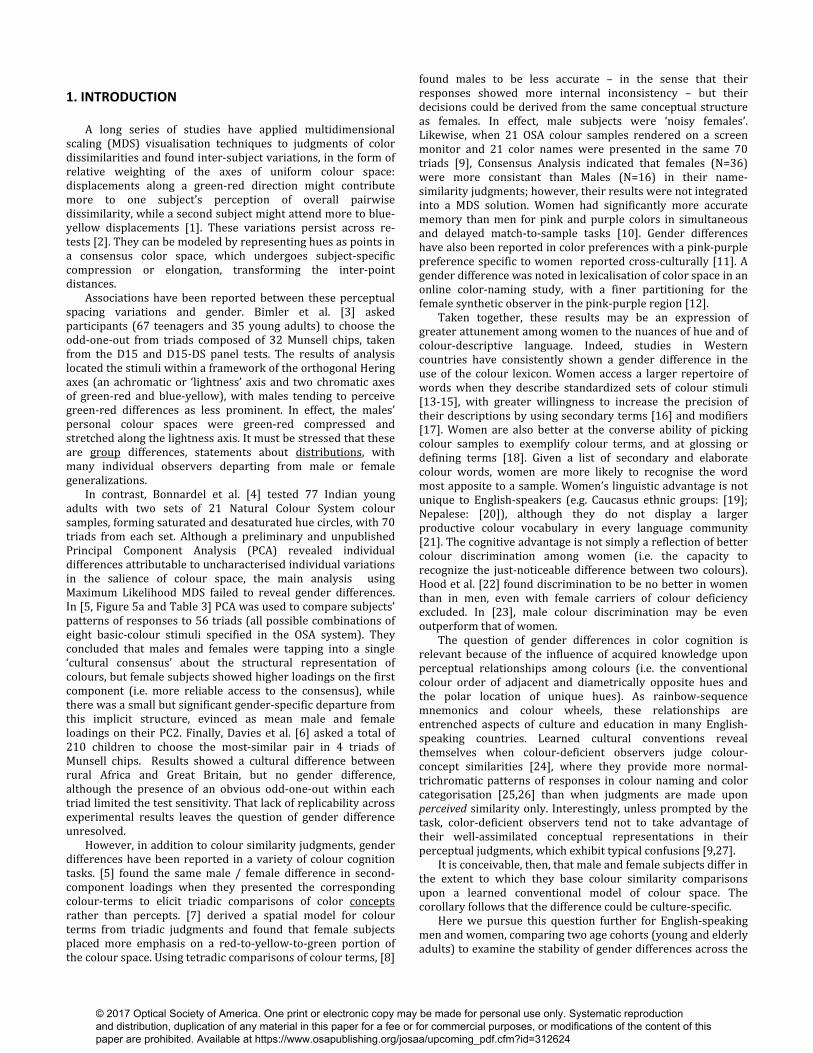
life-span. Stimuli were Munsell color samples at a constant lightness level, with the maximum chroma at each equally-spaced hue. Thus they form an oval rather than a circle in the CIELAB uniform-chromaticity scale diagram, with its major axis of elongation running from purple (smallest chroma) to yellow/green (highest chroma) (Figure 1). The color-space distance between some successive pairs are increased, either by an increment in saturation (e.g. between 2.5G / 8 and 7.5 GY / 10) or because both colors are saturated and far from the origin (e.g. 2.5Y / 12 and 7.5Y / 12). We speculate that in this task of judging dissimilarities, where difficulty is increased by a large scale of dissimilarities including more than one dimension, subjects may ignore these complications and augment their judgments with propositional knowledge that red and green are diametrical opposites, equal in dissimilarity to blue and yellow. To the extent that observers draw upon a simple colour-circle model, they will underestimate colour-space distances along the major axis of the CIELAB pseudo-ellipse, and exaggerate them along its minor axis. One can further speculate that stimuli including saturated, relatively namable colors might evoke conventional knowledge about their relationships. Data are processed with Principal Component Analysis and two forms of Multidimensional scaling to focus on the emergent consensus knowledge about colour space as such, and on departures from that consensus as functions of age and gender. 2. METHOD

A. Subjects Fifty younger subjects (25 F), aged between 18 and 30, were psychology students at the University of Sunderland. They received course credit for their participation. A total of 105 were recruited for this study. Fifty-four older subjects (28 F), aged between 70 and 84, were approached while registering to attend an open lecture at the University of Sunderland, or had previously taken part in a study at the University. A large proportion of them were members of the Sunderland Third Age University. Written informed consents were obtained in line with the Tenets of Helsinki, and the study had the approval of the Ethic Committee of the University of Sunderland. Participants’ colour vision was tested with Ishihara pseudo-isochromatic plates, and one male was classified as a colour deficient; his data were excluded from the results. Participants from the older age group were given a questionnaire about cataract affliction: 33 were unaffected; 11 reported a low level of cataract either mono or binocularly; one reported a medium level in one eye and nine had undergone cataract removal surgery.

Figure 1. Locations of the stimuli in the CIE-a*b* diagram. B. Stimuli

Twenty Munsell chips were taken from the Glossy edition, spaced at 20 equal steps around the colour circle, with two chips from each of the 10 sectors of the circle in the Munsell system (Hue designations 2.5 and 7.5 within each sector). 5PB was added as the 21st stimulus. All chips had the same lightness (Value = 8) but were selected with the highest available saturation for each hue, so they ranged in saturation from Chroma = 4 (for the purple and blue-green region) up to Chroma = 12 (for the yellow to green-yellow region). As noted, not all color categories were represented by ideal examples. A list of 70 triads was prepared, following a Balanced Incomplete Design or BID [28] with λ=1: that is, each pair of stimuli appeared in one and only one triad. The 70 triads thus include all 210 possible pairs. Each triad was three different stimuli and each stimulus appeared in 10 triads. C. Procedure Triads were displayed in a triangular arrangement on a large table of a uniform-grey surface (equivalent to Munsell Neutral N/5). A ceiling panel (Verivide luminaire 120) provided a D65 illuminant with a reflected light intensity of 150 cd/m2. Subjects indicated the least-similar or odd-one-out stimulus of the three, with one experimenter recording their choice, while a second experimenter prepared the stimuli for the next triad. Triads were presented in a randomised sequence, the same sequence for all subjects. No time constraint was imposed, and subjects generally performed the task within 15 minutes.


Using an index m to specify subjects, the m-th subject’s responses were encoded as the lower triangle of a 21-by-21 matrix of estimated similarities, Sm. A given matrix element smij was 1 if the i-th and j-th stimuli were most similar in the triad in which that pair appeared together, and 0 if either stimulus i or j was the odd-one-out in that triad. Thus each lower triangle contains 70 ‘1’ elements and 140 ‘0’ elements. D. Analysis We followed two complementary approaches to summarize the data. To examine the data for forms of systematic inter-subject variation (i.e. variations significantly associated with age or gender), we wrote each subject’s responses as a column of 1s and 0s – vectorising the lower half of the Sm matrix – and subjected the 210-by-104 data table to PCA. Here we follow [5] who applied PCA as the first stage of Cultural Consensus Theory [29]. Note that this is the ‘Q mode’ of PCA, in which subjects rather than items are the unit of analysis, so that each component is a prototypical pattern of responses from an idealized subject. If subjects converge upon a consensus about the perceptual structure (i.e. the relationships among the stimuli), so that any two subjects are closely correlated in their responses, this structure emerges from PCA (in its Q-mode) as the first unrotated component PC1, the ‘g-factor’. Each subject’s loading on PC1 measures his or her ‘competence’ or access to the consensus. Second, MDS was used to provide a geometrical framework in which to interpret any individual differences that might emerge. The outcomes of MDS are a collective spatial model with a specified number of dimensions, integrating similarity judgements from all participants, and also models for any given subgroup of subjects. MDS arranges points, representing the stimuli, so that the distances between them reflect the corresponding inter-stimulus similarities. If two colours in a triad are consistently chosen as the most similar pair, then those two points should be neighbors in the space, with the point for the odd-one-out located farther away. Classical MDS was used first, to visualize ‘synthetic similarity data’ derived from the components obtained in PCA (see result section); then a maximum-likelihood MDS algorithm (the MTRIAD program, as in [3,4]) was applied to the raw responses to provide a stable solution when classical MDS is impaired by the sparse nature of triads in the BID. An independent implementation, coded in the OpenSource statistical computing / graphics environment R, gave identical results (K. Knoblauch, pers. comm.). 3. RESULTS In the cultural consensus model [29], estimates of the individual subjects’ competence or knowledge are provided by their loading values on the first component extracted from their responses by Q-mode PCA. Here PC1 accounted for 59.6% of variance, while PC2 and PC3 were much smaller, accounting for 3.8% and 3.3% respectively (eigenvalues were almost identical to variance percentage). Subsequent components can be treated as noise; their contributions to variance dropped to 1.9% for PC4, then leveled off (the usual criteria for the significance of components assume data to be normally distributed and are not applicable to the present binary-encoded responses). The mean loading on PC1 was 0.767, reflecting the strength of the shared

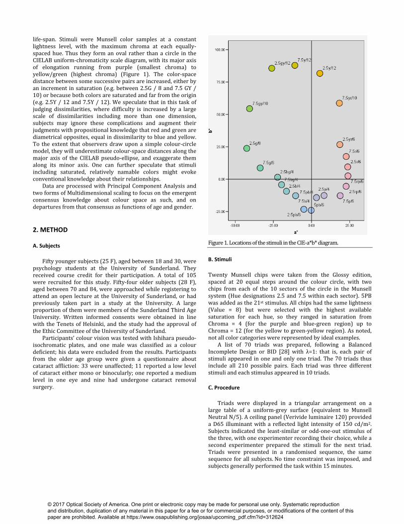
perceptual structure. That is, about 77% of the colour-similarity structure was shared across all participants. The remaining 23% consists of error variance, plus individual differences which could be unique to each subject, or could be systematic response styles, specific to age or sex or an interaction (or other variables not identified here). Three male subjects (one in the younger and two in the older age bands) departed from the consensus and had small or negative PC1 loadings; they were idiosyncratic or simply unreliable informants. Their data were excluded from subsequent analysis, after checking that statistical tests were not affected by the omission. An analysis of variance revealed that PC1 loadings were significantly higher in younger compared to older adults, with mean values 0.792 and 0.740 respectively (F[1,98] =9.19, p = .003, η2 = 0.087), and for females compared to males, with means 0.787 and 0.744 respectively (F[1,98] =6.35, p = .013, η2 = 0.062) (Figure 2a). That is, youth and femaleness both tended to make one a more reliable judge of colour similarity, with better access to the consensus. There was no significant interaction between Age and Gender. Male agreement was still relatively low as measured by their PC1 loadings from applying PCA to male data only. That is, they diverged not only from the combined consensus, but also from a gender-specific consensus.

Figure 2. Mean loadings on principal components PC1 (top) and PC3 (bottom) as a function of age band and gender. Error bars correspond to 95% confidence interval.

20+ 70+

Mea

n lo

adin

g PC

1

20+ 70+

Mea

n lo

adin

g PC

3


Figure 3. Distributions of PC1 vs. PC3 loadings per age group and gender. For PC3, females had significantly lower loadings than males, with means of -0.057 and 0.073 respectively (F[1.98] =14.90, p ≤ .001, η2 = 0.134). There was no significant age difference, but a significant interaction between Age and Gender (F[3,96] = 6.30, p = .014, η2 = 0.062) means that the gender difference was significant in the older adult (t (49) = -0.452 , p < 0.001) but not in the younger group, as if accentuated with age. These associations are evident in a plot of individual loadings on PC3 against PC1 (Figure 3). ANOVA of the PC2 loadings revealed no significant effect of age or gender.

Figure 4. Two-dimensional MDS solutions for synthetic similarity matrices S3- and S3+ corresponding to PC1 with negative (top) and positive (bottom) contributions of PC3. To determine the nature of this gender difference requires one to interpret PC3 itself. As noted, each component can be regarded as a prototypal or idealized pattern of estimated inter-colour similarities, with PC1 as the ‘cultural consensus’. We recovered and saved the scores comprising each component. Because each component is formatted in the same way as the individual columns of data (i.e. a 210-vector corresponding to the ‘unwrapped’ version of a similarity matrix), its scores can be treated as a matrix for analysis with standard non-metric MDS. Note that the ML-MDS algorithm (used below) operates on comparisons and so is not appropriate for the present purpose.

PC1

PC3


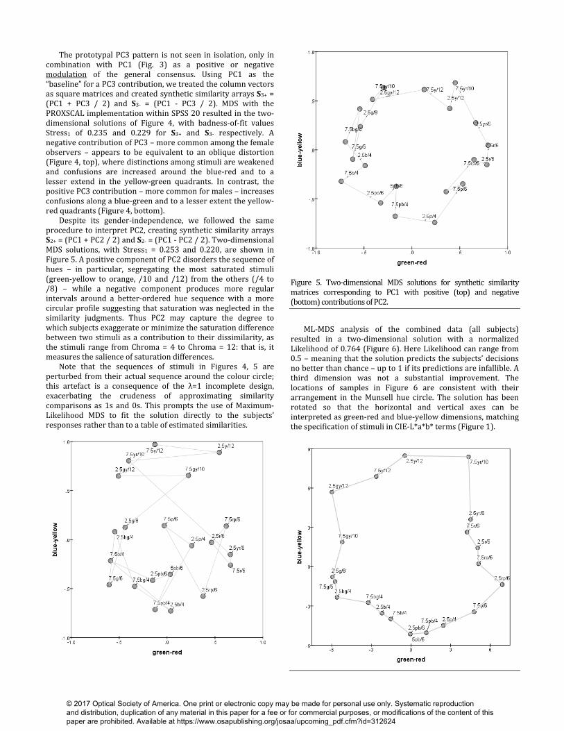
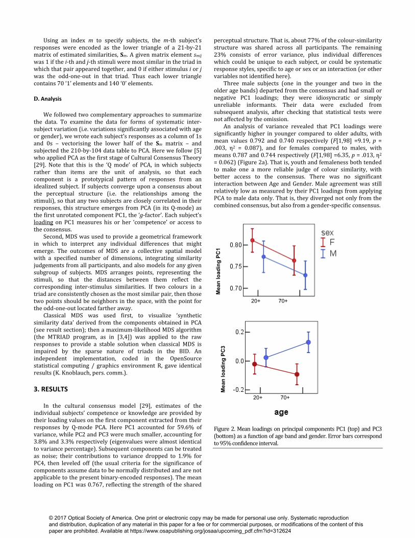
The prototypal PC3 pattern is not seen in isolation, only in combination with PC1 (Fig. 3) as a positive or negative modulation of the general consensus. Using PC1 as the “baseline” for a PC3 contribution, we treated the column vectors as square matrices and created synthetic similarity arrays S3+ = (PC1 + PC3 / 2) and S3- = (PC1 - PC3 / 2). MDS with the PROXSCAL implementation within SPSS 20 resulted in the two-dimensional solutions of Figure 4, with badness-of-fit values Stress1 of 0.235 and 0.229 for S3+ and S3- respectively. A negative contribution of PC3 – more common among the female observers – appears to be equivalent to an oblique distortion (Figure 4, top), where distinctions among stimuli are weakened and confusions are increased around the blue-red and to a lesser extend in the yellow-green quadrants. In contrast, the positive PC3 contribution – more common for males – increases confusions along a blue-green and to a lesser extent the yellow-red quadrants (Figure 4, bottom). Despite its gender-independence, we followed the same procedure to interpret PC2, creating synthetic similarity arrays S2+ = (PC1 + PC2 / 2) and S2- = (PC1 - PC2 / 2). Two-dimensional MDS solutions, with Stress1 = 0.253 and 0.220, are shown in Figure 5. A positive component of PC2 disorders the sequence of hues – in particular, segregating the most saturated stimuli (green-yellow to orange, /10 and /12) from the others (/4 to /8) – while a negative component produces more regular intervals around a better-ordered hue sequence with a more circular profile suggesting that saturation was neglected in the similarity judgments. Thus PC2 may capture the degree to which subjects exaggerate or minimize the saturation difference between two stimuli as a contribution to their dissimilarity, as the stimuli range from Chroma = 4 to Chroma = 12: that is, it measures the salience of saturation differences. Note that the sequences of stimuli in Figures 4, 5 are perturbed from their actual sequence around the colour circle; this artefact is a consequence of the λ=1 incomplete design, exacerbating the crudeness of approximating similarity comparisons as 1s and 0s. This prompts the use of Maximum-Likelihood MDS to fit the solution directly to the subjects’ responses rather than to a table of estimated similarities.

Figure 5. Two-dimensional MDS solutions for synthetic similarity matrices corresponding to PC1 with positive (top) and negative (bottom) contributions of PC2. ML-MDS analysis of the combined data (all subjects) resulted in a two-dimensional solution with a normalized Likelihood of 0.764 (Figure 6). Here Likelihood can range from 0.5 – meaning that the solution predicts the subjects’ decisions no better than chance – up to 1 if its predictions are infallible. A third dimension was not a substantial improvement. The locations of samples in Figure 6 are consistent with their arrangement in the Munsell hue circle. The solution has been rotated so that the horizontal and vertical axes can be interpreted as green-red and blue-yellow dimensions, matching the specification of stimuli in CIE-L*a*b* terms (Figure 1).


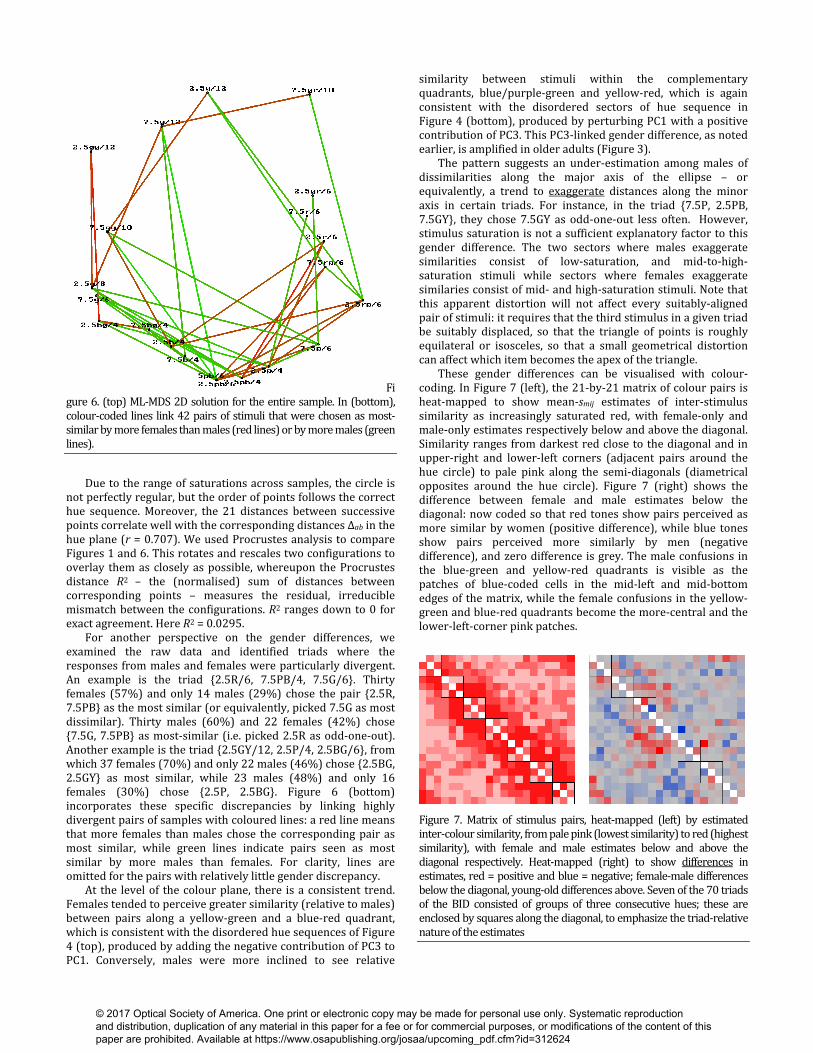
Figure 6. (top) ML-MDS 2D solution for the entire sample. In (bottom), colour-coded lines link 42 pairs of stimuli that were chosen as most-similar by more females than males (red lines) or by more males (green lines). Due to the range of saturations across samples, the circle is not perfectly regular, but the order of points follows the correct hue sequence. Moreover, the 21 distances between successive points correlate well with the corresponding distances Δab in the hue plane (r = 0.707). We used Procrustes analysis to compare Figures 1 and 6. This rotates and rescales two configurations to overlay them as closely as possible, whereupon the Procrustes distance R2 – the (normalised) sum of distances between corresponding points – measures the residual, irreducible mismatch between the configurations. R2 ranges down to 0 for exact agreement. Here R2 = 0.0295. For another perspective on the gender differences, we examined the raw data and identified triads where the responses from males and females were particularly divergent. An example is the triad {2.5R/6, 7.5PB/4, 7.5G/6}. Thirty females (57%) and only 14 males (29%) chose the pair {2.5R, 7.5PB} as the most similar (or equivalently, picked 7.5G as most dissimilar). Thirty males (60%) and 22 females (42%) chose {7.5G, 7.5PB} as most-similar (i.e. picked 2.5R as odd-one-out). Another example is the triad {2.5GY/12, 2.5P/4, 2.5BG/6}, from which 37 females (70%) and only 22 males (46%) chose {2.5BG, 2.5GY} as most similar, while 23 males (48%) and only 16 females (30%) chose {2.5P, 2.5BG}. Figure 6 (bottom) incorporates these specific discrepancies by linking highly divergent pairs of samples with coloured lines: a red line means that more females than males chose the corresponding pair as most similar, while green lines indicate pairs seen as most similar by more males than females. For clarity, lines are omitted for the pairs with relatively little gender discrepancy. At the level of the colour plane, there is a consistent trend. Females tended to perceive greater similarity (relative to males) between pairs along a yellow-green and a blue-red quadrant, which is consistent with the disordered hue sequences of Figure 4 (top), produced by adding the negative contribution of PC3 to PC1. Conversely, males were more inclined to see relative

similarity between stimuli within the complementary quadrants, blue/purple-green and yellow-red, which is again consistent with the disordered sectors of hue sequence in Figure 4 (bottom), produced by perturbing PC1 with a positive contribution of PC3. This PC3-linked gender difference, as noted earlier, is amplified in older adults (Figure 3). The pattern suggests an under-estimation among males of dissimilarities along the major axis of the ellipse – or equivalently, a trend to exaggerate distances along the minor axis in certain triads. For instance, in the triad {7.5P, 2.5PB, 7.5GY}, they chose 7.5GY as odd-one-out less often. However, stimulus saturation is not a sufficient explanatory factor to this gender difference. The two sectors where males exaggerate similarities consist of low-saturation, and mid-to-high-saturation stimuli while sectors where females exaggerate similaries consist of mid- and high-saturation stimuli. Note that this apparent distortion will not affect every suitably-aligned pair of stimuli: it requires that the third stimulus in a given triad be suitably displaced, so that the triangle of points is roughly equilateral or isosceles, so that a small geometrical distortion can affect which item becomes the apex of the triangle. These gender differences can be visualised with colour-coding. In Figure 7 (left), the 21-by-21 matrix of colour pairs is heat-mapped to show mean-smij estimates of inter-stimulus similarity as increasingly saturated red, with female-only and male-only estimates respectively below and above the diagonal. Similarity ranges from darkest red close to the diagonal and in upper-right and lower-left corners (adjacent pairs around the hue circle) to pale pink along the semi-diagonals (diametrical opposites around the hue circle). Figure 7 (right) shows the difference between female and male estimates below the diagonal: now coded so that red tones show pairs perceived as more similar by women (positive difference), while blue tones show pairs perceived more similarly by men (negative difference), and zero difference is grey. The male confusions in the blue-green and yellow-red quadrants is visible as the patches of blue-coded cells in the mid-left and mid-bottom edges of the matrix, while the female confusions in the yellow-green and blue-red quadrants become the more-central and the lower-left-corner pink patches.

Figure 7. Matrix of stimulus pairs, heat-mapped (left) by estimated inter-colour similarity, from pale pink (lowest similarity) to red (highest similarity), with female and male estimates below and above the diagonal respectively. Heat-mapped (right) to show differences in estimates, red = positive and blue = negative; female-male differences below the diagonal, young-old differences above. Seven of the 70 triads of the BID consisted of groups of three consecutive hues; these are enclosed by squares along the diagonal, to emphasize the triad-relative nature of the estimates © 2017 Optical Society of America. One print or electronic copy may be made for personal use only. Systematic reproduction and distribution, duplication of any material in this paper for a fee or for commercial purposes, or modifications of the content of this paper are prohibited. Available at https://www.osapublishing.org/josaa/upcoming_pdf.cfm?id=312624

When we fit ML-MDS solutions to the male and female responses separately (Figure 8), the normalised Likelihood values were 0.728 and 0.774 respectively, indicating greater internal consistency among females. The same general structure is present in both solutions. However, the female perceptual space displays less angularity and greater regularity, especially in the upper half, and this subjective impression is borne out by the correlation of r = 0.716 between the 21 distances between successive hues in the female solution and corresponding distances Δab(i,j) in Figure 1, compared to r = 0.647 for the male solution. The female solution was also a closer match to locations of stimuli in the CIEL*a*b* plane (R2 = 0.0266) than the male solution was (R2 = 0.0388), so by that standard female responses were collectively more veridical. Relative to the a*b* stimulus attributes, both solutions are distorted, but the male solution is more so.

Figure 8. Separate ML-MDS solutions for males (top) and females (bottom). Separate solutions for responses from younger and older adults are shown in Figure 9. The former group showed more internal consistency, with normalised Likelihoods of 0.775 and 0.729 respectively. Procrustes analysis indicated little difference between the solutions in how well they reproduce the arrangement of hues in colour space (R2 = 0.0334 and R2 = 0.0323 for younger and older adults). Compared to young adults, no impairment in older adult’s collective similarity judgements for supra-theshold colour as judged by inter-point distances. Successive distances around the hue sequence derived from younger adults’ data were less-well correlated with CIELAB colour-plane distances Δab(i, j) (r = 0.572) than in the older-adults solution (r = 0.714). If we interpret the slightly lower PC1 loadings among the older cohort as an index of increased fluctuation from the consensus, those increased errors have not reached the point of disordering the hue sequence, i.e. the group compromise from which they vary remains recognisable. The older adults’ space appears to show a relative compression along the green-red axis. This may be an illusion, however, with only one or two points (e.g. 7.5GY/10 and 7.5 R/ 6) displaced towards the centre. The dispersal of coordinates along the horizontal and vertical axes is the same in both solutions. We examined the raw data to identify the triads and stimulus pairs showing greatest young / old difference, but no systematic pattern emerged. Figure 7 (right) shows sporadic red and blue squares of differences above the diagonal, but no coherent structure. 4. DISCUSSION A preliminary note is in order about the forms of MDS analysis available to extract colour spaces from odd-one-out judgements. A standard practice is to treat the smij values as low-resolution estimates of inter-stimulus similarity, grist for the mill of MDS (e.g. [30]). This ignores the within-triad specificity of each comparison, and makes an implicit assumption that the 140 stimulus pairs with smij = 0 values (from subject m) are all more dissimilar than the 70 pairs with smij = 1: this assumption is not correct as each triad represents a different geometry in the colour plane. The problem is evident here when we took this approach to produce Figures 4 and 5, which interpret the principal components by combining them in synthetic similarity matrices. The resulting artifacts include the zig-zag ‘backtracking’ of the sequences of colours, and the displacement of some stimuli into the interiors of the solutions when they should lie on the pseudo-elliptical perimeter.


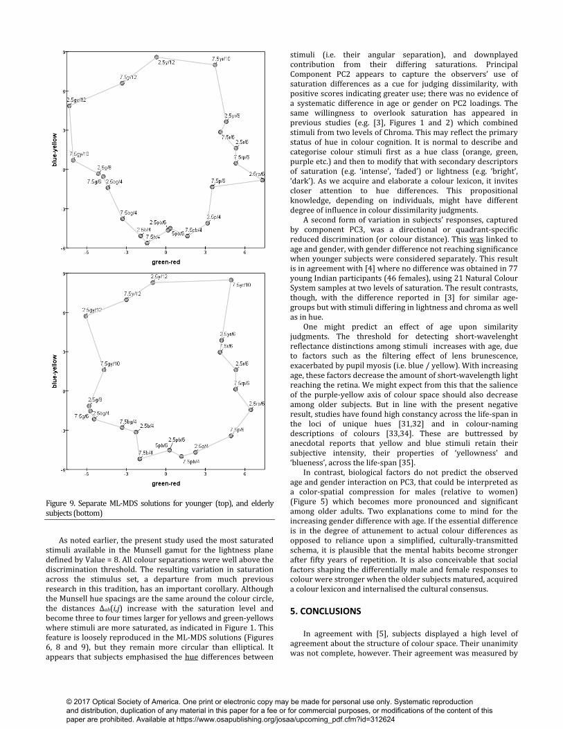
Figure 9. Separate ML-MDS solutions for younger (top), and elderly subjects (bottom) As noted earlier, the present study used the most saturated stimuli available in the Munsell gamut for the lightness plane defined by Value = 8. All colour separations were well above the discrimination threshold. The resulting variation in saturation across the stimulus set, a departure from much previous research in this tradition, has an important corollary. Although the Munsell hue spacings are the same around the colour circle, the distances Δab(i,j) increase with the saturation level and become three to four times larger for yellows and green-yellows where stimuli are more saturated, as indicated in Figure 1. This feature is loosely reproduced in the ML-MDS solutions (Figures 6, 8 and 9), but they remain more circular than elliptical. It appears that subjects emphasised the hue differences between

stimuli (i.e. their angular separation), and downplayed contribution from their differing saturations. Principal Component PC2 appears to capture the observers’ use of saturation differences as a cue for judging dissimilarity, with positive scores indicating greater use; there was no evidence of a systematic difference in age or gender on PC2 loadings. The same willingness to overlook saturation has appeared in previous studies (e.g. [3], Figures 1 and 2) which combined stimuli from two levels of Chroma. This may reflect the primary status of hue in colour cognition. It is normal to describe and categorise colour stimuli first as a hue class (orange, green, purple etc.) and then to modify that with secondary descriptors of saturation (e.g. ‘intense’, ‘faded’) or lightness (e.g. ‘bright’, ‘dark’). As we acquire and elaborate a colour lexicon, it invites closer attention to hue differences. This propositional knowledge, depending on individuals, might have different degree of influence in colour dissimilarity judgments. A second form of variation in subjects’ responses, captured by component PC3, was a directional or quadrant-specific reduced discrimination (or colour distance). This was linked to age and gender, with gender difference not reaching significance when younger subjects were considered separately. This result is in agreement with [4] where no difference was obtained in 77 young Indian participants (46 females), using 21 Natural Colour System samples at two levels of saturation. The result contrasts, though, with the difference reported in [3] for similar age-groups but with stimuli differing in lightness and chroma as well as in hue. One might predict an effect of age upon similarity judgments. The threshold for detecting short-wavelenght reflectance distinctions among stimuli increases with age, due to factors such as the filtering effect of lens brunescence, exacerbated by pupil myosis (i.e. blue / yellow). With increasing age, these factors decrease the amount of short-wavelength light reaching the retina. We might expect from this that the salience of the purple-yellow axis of colour space should also decrease among older subjects. But in line with the present negative result, studies have found high constancy across the life-span in the loci of unique hues [31,32] and in colour-naming descriptions of colours [33,34]. These are buttressed by anecdotal reports that yellow and blue stimuli retain their subjective intensity, their properties of ‘yellowness’ and ‘blueness’, across the life-span [35]. In contrast, biological factors do not predict the observed age and gender interaction on PC3, that could be interpreted as a color-spatial compression for males (relative to women) (Figure 5) which becomes more pronounced and significant among older adults. Two explanations come to mind for the increasing gender difference with age. If the essential difference is in the degree of attunement to actual colour differences as opposed to reliance upon a simplified, culturally-transmitted schema, it is plausible that the mental habits become stronger after fifty years of repetition. It is also conceivable that social factors shaping the differentially male and female responses to colour were stronger when the older subjects matured, acquired a colour lexicon and internalised the cultural consensus. 5. CONCLUSIONS In agreement with [5], subjects displayed a high level of agreement about the structure of colour space. Their unanimity was not complete, however. Their agreement was measured by


values on the first Principal Component of the responses, and showed effects of gender and age (Fig 2, top). Crucially, when the odd-one-out judgements of individual subjects departed from the broad cultural consensus, these deviations were not random fluctuations, but evinced an element of structure: sub-populations of subjects followed coherent trends, producing the second and third principal components of the PCA solution. The second component, for instance, can tentatively be attributed to a mode of variation in which subjects varied in the degree to which they attend to or ignore differences in the saturation of stimuli as a contribution to their pairwise dissimilarities. Another form of subject variation, captured by the third component, was associated with gender: evidence that it is not merely an artifact. The gender difference in perceived colour similarities can be described as a quadrant-specific distortion of distances in colour space, more apparent in some sectors of the colour plane than in others. Figures 6 and 7 indicate that relative to the consensus, the male observers collectively reported a reduction of numerous distances among an orange-red-purple range of hues, and (on the other side of the hue circle), among a green-cyan-blue range; conversely, females experienced contraction of dissimilarities among a blue-purple range, and among a chartreuse-yellow-orange range. That is, for each colour pair thus affected, one gender tended to choose the third colour in that triad as odd-one-out, more often than the other gender did, exaggerating the dissimilarity across the circle between it and the first two colours. This is apparent in responses to specific triads. One could also characterise this as an overall global compression of the colour plane relative to the CIELAB locations of the stimuli, so as to make their arrangement less elliptical, this expectation of a circular arrangement being stronger in males than in females. This is in keeping with the lower awareness among males of the actual nuances of colour (so their ML-MDS solution provides a poorer approximation of CIELAB locations) as well as their lower attunement to the colour-similarity consensus (i.e. their lower loadings on PC1). Thus rather than aligning with conventional or cardinal dimensions of colour description, the compression axes that generate individual solutions, and distinguish males from females, are determined by the major and minor axes of the ellipse of selected stimuli.This account predicts that subjects will not display the same gender-specific tendency to treat a color ellipse as circular if the convention of the schematic color circle or ‘compass’ is not as prominent in their cultural and educational background as it is in the UK (e.g. [4]). However, it does not accommodate the earlier report of red-green color-space compression among New Zealand males [3], where the veridical arrangement of hues was not notably elliptical, either in Munsell terms or in the CIELAB plane. If there is a single social-psychology phenomenon underlying all the observations, we are not yet in a position to describe it in detail. References

1. J.D. Carroll and J.-J. Chang, “Analysis of Individual Differences in Multidimensional scaling via an N-way generalization of ‘Eckart-Young’ Decomposition,” Psychometrika 35, 283–319 (1970).

2. G.V. Paramei, D. Bimler, and N.O. Mislavskaia, “Color perception in twins: individual variation beyond common genetic inheritance”, Clinical & Experimental Optometry, 87, 305-312 (2004).

3. D. Bimler, J. Kirkland, and Jameson, K., “Quantifying variations in personal color spaces: Are there sex differences in color vision?” Col.Res.Appl., 29, 128-134 (2004).

4. V. Bonnardel, S. Beniwal, N. Dubey, M. Pande, K. Knoblauch, and D. Bimler, “Perceptual color spacing derived from Maximum Likelihood multidimensional scaling,” JOSA A, 33, A30-36 (2016).

5. C.C. Moore, A.K. Romney, and T.-L. Hsia, “Cultural, gender, and individual differences in perceptual and semantic structures of basic colors in Chinese and English,” J. Cogn. Culture, 2, 1-28 (2002).

6. I.R. Davies, S.K. Boyles, and A. Franklin, “Men and women from ten language-groups weight colour cardinal axes the same,” Perception, 34, S158 (2005).

7. N.L. Furbee, K. Maynard, J.J. Smith, R.A. Benfer, S. Quick, and L. Ross, “The emergence of color cognition from color perception,” Journal of Linguistic Anthropology, 6, 223-240 (1997).

8. L.D. Griffin, “Males are ‘noisy females’ when it comes to reporting the psychological structure of the basic colours,” Perception, 32, S387 (2002).

9. B. Sayim, K.A. Jameson, N. Alvarado, and M.A. Szeszel, “Semantic and perceptual representations of color: Evidence of a shared color naming function,” J. Cogn. Culture, 5, 165-220 (2005).

10. V. Bonnardel & J. Herrero, “Memory for colours: a reaction time experiment,” Proceedings of the Third European Conference on Colour in Graphics, Imaging, and Vision, 110-115, Leeds, UK. (2006).

11. V. Bonnardel, S. Beniwal, N. Dubey, M. Pande, M., and D. Bimler, “Gender difference in color preference across cultures: An archetypal pattern modulated by a female cultural stereotype,” Col.Res. Appl. DOI 10.1002/col.22188 (2017).

12. G. V. Paramei, Y. A. Griber & D. Mylonas, “An online color naming experiment in Russian using Munsell color samples,” Col.Res. Appl. DOI 10.1002/col.22190 (2017).

13. E. Rich, “Sex-related differences in colour vocabulary,” Language & Speech, 20, 404-409 (1977).

14. J. Simpson and A.W.S. Tarrant, “Sex- and age-related differences in colour vocabulary,” Language & Speech, 34, 57-62 (1991).

15. D. Mylonas, G.V. Paramei, and L.MacDonald, “Gender differences in colour naming,” In Anderson, W., Biggam, C.P., Hough, C. & Kay, C. (Eds), Colour studies: A broad spectrum (pp. 225-239). Amsterdam: John Benjamins (2014).

16. K. Greene, and M. Gynther, “Blue versus periwinkle: Color identification and gender,” Perceptual & Motor Skills, 80, 27-32 (1995).

17. V. Bonnardel, S. Miller, L.Wardle & E. Drews “Gender differences in colour naming.,” Perception, 31, 71a. (2002).

18. R.H. Nowaczyk, “Sex-related differences in the color lexicon,” Language & Speech, 25, 257-265 (1982).

19. L.V.Samarina, “Gender, age and descriptive color terminology in some Caucasus cultures,” In MacLaury, R.E., Paramei, G.V., & Dedrick, D. (Eds), Anthropology of Color: Interdisciplinary Multilevel Modeling (pp. 257-266). Amsterdam: John Benjamins (2007).

20. L.L. Thomas, A.T. Curtis, and R. Bolton, “Sex differences in elicited color lexicon size,” Perceptual & Motor Skills, 47, 77-78 (1978).

21. D.L. Bimler and M. Uusküla, “From listing data to semantic maps: cross-linguistic commonalities in cognitive representation of colour,” Folklore: Electronic Journal of Folklore, 64. 57-90 (2016).

22. S.M. Hood, J.D. Mollon, L. Purves, and G. Jordan, “Color discrimination in carriers of color deficiency,” Vision Research, 26, 2894-2900 (2006).

23. Rodríguez-Camona, M., Sharpe, L.T., Harlow, J.A., and Barbur, J.L. (2008). Sex-related differences in chromatic sensitivity. Visual Neurosci., 25, 433-440.

24. R. N. Shepard, and L. A. Cooper, “Representation of colors in the blind, colorblind, and normally sighted,” Psychol. Sci., 3, 97-104 (1992).

25. V. Bonnardel, “Color naming and categorization in inherited color vision deficiencies,” Visual Neurosci., 23, 637-634 (2006).


26. J. Lillo, H. Moreira, L. Álvaro, and I. Davies, “Use of basic color terms by red-green dichromats: 1. General description,” Col. Res. & Appl., 39, 360-371 (2014).

27. D. Jameson and L. M. Hurvich, “Dichromatic color language: ‘Reds’ and ‘Greens’ don’t look alike but their colors do,” Sensory Processes, 2, 146-155 (1978).

28. M.L. Burton and S.B. Nerlove, “Balanced designs for triads tests: Two examples from English,” Social Science Research, 5, 247-267 (1976).

29. A. K. Romney, C. C. Moore, W. H. Batchelder, and T-L. Hsia, “Statistical methods for characterizing similarities and differences between semantic structures,” Proceedings of the National Academy of Sciences, 97, 518-523 (2000).

30. A.K. Romney, D.D. Brewer, and W.H. Batchelder, “Predicting clustering from semantic structure,” Psychol. Sci., 4, 28-34 (1993).

31. L. Beke, G. Kutas, Y. Kwak, G.Y. Sung, D.-S. Park, and P. Bodrogi, Color preference of aged observers compared to young observers. Col.Res.Appl., 33, 381-394 (2008).

32. B.E. Schefrin and J.S. Werner, “Loci of spectral unique hues throughout the life span,” JOSA A, 7, 305-311 (1990).

33. B.E. Schefrin and J.S. Werner, “Age-related changes in the colour appearance of broadband surfaces,” Col.Res.Appl., 18, 380-389 (1993).

34. J.L. Hardy, C.M. Frederick, P. Kay, and J.S. Werner, “Color naming, lens aging, and grue: What the optics of the aging eye can teach us about color,” Psychol.Sci., 16, 321-327 (2005).

35. W.D. Wright, “Talking about color,” Col.Res.Appl., 13, 138-139 (1988).


age and gender effects on perceptual colour scaling using

Documents