i n

Q-

BO o Q

<

<

D

AGARDograph 54

« • • *

r -: * •

AGARDograph

W 'V WIND TUNNEL

CALIBRATION TECHNIQUES

by

A. POPE

APRIL 1961

AGARDograph 54

NORTH ATLANTIC TREATY ORGANIZATION

ADVISORY GROUP FOR AERONAUTICAL RESEARCH AND DEVELOPMENT

WIND-TUNNEL CALIBRATION TECHNIQUES

by

Alan Pope

SANDIA CORPORATION

April 1961

SUMMARY

This paper discusses air-flow measuring instruments, their use, and the manner of working up and presenting the data obtained when calibra­ting low-speed, nearsonic, transonic, supersonic, and hypersonic wind tunnels.

SOMMAIRE

Cette etude analyse les instruments destines a la mesure de 1'ecoule­ment de 1'air, ainsi que leur emploi et la maniere d'exploiter et de presenter les renseignements obtenus lors de 1' etalonnage de souffleries a basse vitesse, en subsonique elev£, transonique, supersonique et hypersonique.

533.6.071.4 3b8c

ii

CONTENTS

Page

SUMMARY ii

LIST OF FIGURES

NOTATION

vi

xi

1. CALIBRATION OF WIND TUNNELS 1 1.1 Introduction 1 1.2 The Measurement of Pressures 2 1.3 Measuring the Temperature of an Airstream 3 1.4 Desirable Flow Quality 5 1.5 Effects of Errors in Measuring 6 1.6 Condensation of Moisture 8

2. CALIBRATION OF LOW-SPEED WIND TUNNELS 11 2.1 General 11 2.2 Speed Setting 11 2.3 Measuring Total Head in a Low-Speed Tunnel 12 2.4 Measuring Static Pressure in a Low-Speed Tunnel 12 2.5 Measuring Temperature in a Low-Speed Tunnel 13 2.6 Determining the Velocity Variation in the Test Section 13 2.7 Determining the Longitudinal Static Pressure Gradient 13 2.8 Determining the Flow Angularity 14 2.9 Turbulence 14 2.10 Large-Scale Flow Fluctuations 15

3. CALIBRATION OF NEARSONIC WIND TUNNELS 17 3.1 General 17 3.2 Setting Mach Number 17 3.3 Measuring Total Head in a Nearsonic Tunnel 18 3.4 Measuring Static Pressure in a Nearsonic Tunnel 18 3.5 Measuring Temperature in a Nearsonic Tunnel 18 3.6 Determining the Mach Number and its Distribution in a

Nearsonic Tunnel 18 3.7 Determining the Flow Angularity 19 3.8 Determining the Longitudinal Static-Pressure Gradient 19 3.9. Determining Turbulence in a Nearsonic Tunnel 19 3.10 Condensation of Moisture 19

4. CALIBRATION OF TRANSONIC WIND TUNNELS 21 4.1 General 21 4.2 Setting Mach Number in a Ventilated Tunnel 21 4.3 Measuring Total Head in a Transonic Tunnel 22 4.4 Measuring Pitot Pressure in a Transonic Tunnel 22 4.5 Measuring Static Pressure in a Transonic Tunnel 23 4.6 Measuring Temperature in a Transonic Tunnel 23

ill

Page

4.7 Determining the Mach Number and its Distribution In a Transonic Tunnel 24

4.8 Determining the Flow Angularity 24 4.9 Determining the Longitudinal Static Pressure Gradient 25 4.10 Determining Turbulence in a Transonic Tunnel 25 4.11 Condensation of Moisture 25 4.12 Wave Cancellation 25

5. CALIBRATION OF SUPERSONIC WIND TUNNELS 27 5.1 General 27 5.2 Setting Mach Number in a Supersonic Tunnel 28 5.3 Measuring Total Head in a Supersonic Tunnel 28 5.4 Measuring Pitot Pressure in a Supersonic Tunnel 28 5.5 Measuring Static Pressure in a Supersonic Tunnel 28 5.6 Measuring Temperature in a Supersonic Tunnel 30 5.7 Determining the Mach Number and its Distribution in a

Supersonic Tunnel 30 5.8 Determining the Flow Angularity 35 5.9 Combined Instruments and Rakes 36 5.10 Determining the Longitudinal Static-Pressure Gradient 36 5.11 Determining Turbulence in a Supersonic Wind Tunnel 37 5.12 Determining Test-Section Noise 39 5.13 Condensation of Moisture 40

6. CALIBRATION OF HYPERSONIC WIND TUNNELS 43 6.1 General 43 6.2 Heating and Liquefaction 44 6.3 Setting Mach Number in a Hypersonic Tunnel 45 6.4 Measuring Total Head in a Hypersonic Tunnel 45 6.5 Measuring the Pitot Pressure in a Hypersonic Tunnel 45 6.6 Measuring Static Pressure in a Hypersonic Tunnel 46 6.7 Measuring Temperature in a Hypersonic Tunnel 47 6.8 Determining Mach Number and its Distribution in a

Hypersonic Tunnel 47 6.9 Determining the Flow Angularity 48 6.10 Determining the Longitudinal Static-Pressure Gradient 49 6.11 Boundary-Layer Surveys 49 6.12 Condensation of Moisture 50

7. THE USE OF CALIBRATION MODELS 51 7.1 General 51 7.2 Model Mounting Effects 51 7.3 Comparison of Data from Several Tunnels 53 7.4 Effect of Errors in Model Dimensions 53 7.5 Comparison of Wind-Tunnel and Flight Data 54

ACKNOWLEDGMENT 54

REFERENCES 55

iv

Page

BIBLIOGRAPHY 60

FIGURES 63

DISTRIBUTION

LIST OF FIGURES

Page

Fig.1.1 Variation of specific gravity of alcohol with temperature 63

Fig.1.2 Variation of specific gravity with temperature of tetrabrome

ethane (TBE) and mercury 64

Pig.1,3 Static pressure for a range of stagnation pressures 65

Fig.1.4 Pitot pressures for a range of stagnation pressures 66

Fig.1.5 Design of stagnation-temperature probe 67

Pig.1.6 Effect of ratio of thermocouple length to diameter for a range

of Mach numbers from 4.90 to 7.60 68 Fig.1.7 Variation of probe temperature recovery factor with free-stream

Reynolds number at various free-stream Mach numbers 69

Fig.1.8 Fall-off of recovery factor with temperature and (secondarily) Mach number. Single-shielded probe, RN = 20,000 69

Pig.1.9 Calibration data for temperature probes to be used in high-temperature settling chambers 70

Pig.1.10 Amount of moisture in atmospheric air at various humidities 71

Pig.1.11 Variation of dewpoint with pressure 72

Fig.2.1 Performance of pitot tube at low Reynolds number. Cylindrical

tube with orifice diameter - 0,64 tube diameter 73

Pig.2.2 Velocity correction for a circular pitot tube near a wall 74

Pig.2.3 Dimensions of a 'standard' pi tot-static tube 75

Pig.2.4 Tip and stem static pressure errors 75

Pig.2,5 Errors in standard pitot-static tube readings produced by yaw 76

Pig.2.6 Static pressure error due to hole size and lip shape,

M = 0.4 to 0.8 77 Fig.2.7 Effect of Mach number on temperature recovery ratio of single-

shielded probe; pt = 2900 lb/in.2, Tt s 140°P; tube diameter =

0.12 inch 78

Pig.2.8 Effect of yaw on temperature recovery factor of single-shielded probe (Same conditions as Fig,2.6) 78

vl

Page

Pig.2.9 Static pipe installation in a subsonic tunnel (Photo by courtesy

ot University of Washington) 79

Pig.2.10 Spherical type yawmeter 80

Pig.2.11 Spherical yawmeter 80

Pig.2.12 Calibration curves for the yawmeter in Fig.2.11 81

Pig.2.13 Turbulence sphere and installation (Photo by courtesy of

University of Washington) 82

Pig.2.14 Turbulence sphere for a 100 m.p.h. tunnel 82

Pig.2.15 Relation between turbulence and turbulence factor 83

Pig.2.16 Chart for estimating most useful diameter for a turbulence

sphere 83 Pig.2.17 Vortex generators which greatly helped a diffusion problem

(Photo by courtesy of University of Wichita) 84 Pig.2.18 Tuft grid for studying large scale fluctuations (Photo by

courtesy of University of Wichita) 85

Pig.3.1 Sensitivities of claw and conical yawmeteps 86

Pig.4.1 Difference between plenum chamber static pressure pc and test

section static pressure p for a number of wall angles # w in minutes 87

Pig.4.2 Total-head tubes (four) and shielded stagnation-temperature

probe in a settling chamber 88

Pig.4.3 Pitot tube in transonic tunnel 89

Pig.4.4 Static pipe in the Sandia 12 inch x 12 inch transonic tunnel 90

Pig.4.5 Plight test data of static pressure probe shown in Pig.5.1 91

Pig.4.6 Calibration plots for a transonic tunnel 92

Fig.4.7 Transducer mounted flush with probe nose for measuring fluctua­tions in pitot pressure 93

Fig.4.8 Variation of stagnation pressure fluctuations, II = 1.1 94

Fig.5.1 Dimensions of supersonic static pressure probe 95

vii

Page

Pig.5.2 Error in Indicated static pressure pm measured in fraction of true static pressure p 96

Fig.5.3 Error in indicated static pressure p measured in fraction of

dynamic pressure q 96

Fig.5.4 Effect of shoulder distance on static pressure reading 97

Fig.5.5 Variation of centerline Mach number with Reynolds number,

40 inch tunnel 98

Fig.5.6 Calibration data from M = 2.0 nozzle 99

Fig.5.7 Contour plot of an M = 3.0 nozzle 100

Pig.5.8 Wave angles for a range of wedge semi-angles 100

Pig.5.9 Wedge dimensions and set-up for angularity measurements 101

Pig.5.10 Sensitivities of several yawmeters at supersonic speeds,

pressure ratio per degree 102 Pig.5.11 Maximum up and down flow in JPL 12-inch supersonic tunnel for

about 0.7 tunnel height up and downstream of resolving center 102

Pig.5.12 Calibration rake 103

Fig.5.13 Dimensions of JPL transition cone 104

Pig. 5.14 Typical determination of transition Reynolds number. Free-stream Reynolds number per foot, 4.31 x 106; transition Reynolds number 3.055 x 106 104

Pig.5.15 Transition Reynolds number on 5° and 10° cones as measured at

several facilities 105

Fig.5.16 Variation of source velocity with tunnel Mach number 106

Pig.5.17 Variation of pressure fluctuation coefficient with Mach number 106

Pig.5.18 Noise emanating from turbulent boundary layer on a missile

model. M = 3.5; RN = 2 x loVinch 107

Pig.6.1 Mach number for equilibrium condensation of air 108

Pig.6.2 Methods of detecting liquefaction in a hypersonic tunnel 109

Pig.6.3 The negligible effect of liquefaction on the normal force

coefficients of an AGARD Model B; M = 8.0 110 viii

Page

Pig.6.4 The negligible effect of liquefaction on the pitching-moment

coefficient of an AGARD Model B 111

Pig.6.5 Effect of Reynolds number on Mach number distribution 112

Pig,6.6 Pitot probe installed in hypersonic test section 113

Pig,6. 7 Summary of data on the effect of model size and shape on

starting 114

Pig.6.8 Static pressure rake with small error 115

Fig.6.9 Diagram of low-pressure manometer 116

Fig.6.10 Elements of McLeod gage 116

Pig.6.11 Measurements of the stagnation temperature along the axis of

the settling chamber of a 6 inch x 6 inch wind tunnel 117 Fig.6,12 Effect of caloric imperfections on total-pressure ratio across

a normal shock wave 118

Fig.6.13 Presentation of Mach number calibration in horizontal plane 119

Fig.6.14 Shadowgraph of flow angularity probe 120

Fig.6.15 Presentation of flow angularity data, M = 7.2 121

Fig.7.1 Typical curve of critical sting length vs. Reynolds number 122

Fig.7.2 The effect of Reynolds number on critical sting length 122

Fig.7.3 Effect of sting to model diameter ratio on base pressure of an ogive-cylinder model; RN = 15 x 106, turbulent boundary layer, M = 2.97 123

Pig,7.4 General configuration of RM-10 (AGARD Model A) research model 123

Fig.7.5 Wind tunnel tests of AGARD Model A under a wide range of

Reynolds numbers (from 4 to 29 x 10*) 124

Fig.7.6 Results from tests of the AGARD Model B in several wind tunnels 125

Fig.7.7 Drawing of AGARD calibration Model B 126

Fig.7.8 Comparison of AGARD Model A data from tests in several tunnels;

H = 1.6, fins off 127 Fig.7.9 Boeing Aircraft Corporation hypersonic research force model 128

ix

Page

Pig.7.10 Comparison of wind-tunnel tests of Boeing hypersonic glider model: slope of normal force curve 129

Fig.7.11 Comparison of wind-tunnel tests of Boeing hypersonic glider model: drag at zero lift 129

Pig.7.12 Comparison of wind-tunnel tests of Boeing hypersonic glider model: slope of drag polar 130

Pig.7.13 Comparison of wind tunnel tests of Boeing hypersonic glider model: slope of pitching-moraent curve 130

Pig.7.14 Comparison of wind-tunnel and flight drag data for AGARD Model A 131

NOTATION

H enthalpy, BTU per lb

M Mach number

Mx local centerline Mach number

M a v average centerline Mach number

Mj index Mach number

L,I length

D model diameter

dg sting diameter

A duct area

Ay vent area

Ae entrance area

p stream static pressure, lb/in 2

p average pressure, lb/in. ?

Pb base pressure, lb/in.2

p m measured pressure, lb/in.2

P r m s root-mean-square pressure, lb/in.2

Pt total or stagnation pressure, lb/in.2

Pt, total pressure ahead of a normal shock, lb/in.2

pt total pressure behind a normal shock, lb/in. 2

y ratio of specific heats

q dynamic pressure, lb/in.2

r recovery factor

Q heat, BTU per lb

Rx recovery factor

T stream static temperature, °R

xi

2

T w wall temperature, °R

Tftw adiabatic wall temperature, R

T measured temperature, °R

Tt total or stagnation temperature, °R

v average velocity, ft/sec.

v r m g root-mean-square velocity, ft/sec.

v„ source velocity, ft/sec.

xii

S E C T I O N 1

CALIBRATION OF WIND TUNNELS

1.1 INTRODUCTION

The calibration of a wind tunnel consists in determining the mean values and uni­formity of various flow parameters in the region to be used for model testing. The parameters basic to any wind-tunnel calibration are stagnation pressure and tempera­ture, velocity or Mach number, and flow angularity. Other flow conditions of interest include static pressure and temperature, turbulence, and the extent of condensation or liquefaction.

Experience over the years has proven that the nozzle to test section flow of air in wind tunnels from the low subsonic to the hypersonic range can be considered isen­tropic when no shock wave, condensation of water vapour, or liquefaction of air exists. This fact has made the job of the wind-tunnel calibrator much easier. By avoiding shocks, condensation and liquefaction, and thus achieving isentropic flow, the total pressure in the test section is equal to the corresponding value when the air is at rest, which can be measured with relative ease in the wind-tunnel settling chamber. Except for heated tunnels where convective losses in the settling chamber become severe, the same is true of temperature. Since the ratios of total pressure and tem­perature to stream quantities are unique functions of Mach number, once settling chamber conditions are known, the calibrator has the choice of measuring any one of the test-section parameters in order to define all the others. The existence of this choice is fortunate because, through the selection of specific parameters in particu­lar speed ranges, one can have superior results, as will be discussed in later sections. Also, no simple, direct method of measuring has been derived for certain of the para­meters such as velocity, static temperature, and Mach number.

Since the complete determination of flow properties in the test section by presently used techniques requires isentropic flow, one of the first problems facing the cali­brator is that of making certain that he has it. This problem is discussed in Section 1.6 and in relevant later pages.

The greatest part of calibration is accomplished through the measurement of pres­sures and temperatures, and general sections covering these measurements follow. However, both the most desirable instruments and the manner of using them change with the speed range of the tunnel and a natural separation for discussing them results, A further advantage of treating calibration by speed range is that this is how a user would want the data presented. The division used herein is as follows:

(a) Low-Speed Wind T u n n e l s . Low-speed tunnels are normally considered to be those which operate in the range where compressibility effects are unimportant, and Reynolds number is a more serious parameter than Mach number. This may be taken as below 300 m.p.h., very few tunnels having been built which go faster than this unless they continue right into the nearsonic (M = 0.95) range.

(b) N e a r s o n i c Wind T u n n e l s . Nearsonic tunnels are those which operate from about M = 0.5 to 0.95 , without ventilated boundaries. In this range (and above),

Mach number becomes a more useful parameter than Reynolds number, and *blocking', particularly near the upper Mach number limit, is of paramount importance. Indeed, few new nearsonic tunnels are expected to be built, due to their severe blocking limitations. However, they do represent a unique type of tunnel, and are hence included.

(c) T r a n s o n i c Wind T u n n e l s . Transonic wind tunnels operate in the range from M = 0.5 to about 1.4. They necessarily have ventilated test sections which ease the blocking problem and, to some extent, the problem of wall reflection of shock waves. Their air should preferably be dried.

(d) S u p e r s o n i c Wind T u n n e l s . Supersonic tunnels operate in the range 1.4 < M < 5.0. In this range, the tunnel air must be dry (dewpoint -40°F or lower); shock waves are usually attached, and their angle is a useful indication of Mach number. Supersonic tunnels cannot achieve a change of Mach number without a nozzle configuration change, usually accomplished by deflecting a flexible plate or changing nozzle blocks. Some stream heating may be necessary at the higher end of the range,

(e) H y p e r s o n i c Wind T u n n e l s . Hypersonic tunnels operate at speeds above M = 5.0. They, also, require a nozzle configuration change for each Mach number, but differ from supersonic tunnels in that considerable heating of the airstream is required if liquefaction of the air is to be avoided as it expands to high Mach number and its local stream temperature drops. Frequently hypersonic tunnels have axisymmetric nozzles.

1.2 THE MEASUREMENT OF PRESSURES

Possibly the most basic and useful tool in the calibration of wind tunnels is the measurement of pressures. The subject is large enough and important enough to justify a report by itself; indeed, there have been many. Accordingly, only a brief comment is included below. The reader is referred to the work of Huppert in Reference 1.1 which gives a summary of the present state of the art. Wind-tunnel pressure measure­ments are made both with fluid columns and with a variety of gages and transducers, with the selection of each determined by the pressure range, desired accuracy, and the response time. Some typical manometer fluids are given in the table below.

Fluid

Water

Alcohol

Dibutyl-phthalate

Tetrabrome ethane

Mercury

Manometer nominal speci f ic gravi ty

0.998 at 70°P

0.8

1.047

2.96

13.54

Remarks

-

See Figure 1.1 for temperature effects

Low boiling point

See Figure 1.2 for temperature effects

See Figure 1.2 for temperature effects

The profusion of gages and transducers defies any short summary, but an important practical suggestion should be noted as follows: in many cases commercial suppliers will select gages of higher than ordinary accuracy upon request. Thus, it may not be necessary to design and build a special instrument just because the ordinary products are not guaranteed to the needed accuracy.

Both static and pitot pressure probe design and calibrations differ with the speed ranges. Data are included in the appropriate sections.

In general probe work, there is a choice between using a single instrument or a rake. The rake has the advantage that all of the data are taken simultaneously - an important point if run time is short, and more data can be taken per run. On the other hand, the single instrument is cheaper and, as discussed later, many blocking problems are eliminated. In general, mutual interference or blocking makes the use of a rake inadvisable except in the transonic and supersonic ranges.

To provide an indication of the magnitude of pressures of concern to calibrators, Figures 1.3 and 1.4 have been prepared from the usual Mach number relations (Ref.1.2), assuming y - 1.4 and a perfect gas. Because of the wide range of pressure measure­ments indicated by the figures, it is clear that techniques useful to some tunnels are quite inapplicable to others.

1.3 MEASURING THE TEMPERATURE OF AN AIRSTREAM

Since any temperature-measuring device (or indeed any device) placed in an air­stream will have a boundary layer on it in which the air is slowed and its temperature raised above the stream temperature, a direct reading of stream static temperature is not possible. To determine the stream temperature, one endeavors to measure the stagnation temperature, Tt , and the stream temperature, T , is then computed from the energy equation*

T = TJ 1 + M2j (1.1)

A device for reading stagnation temperature (or close to it) is called a stagnation-temperature probe. In general, it consists of a thermocouple for reading the tempera­ture, plus an arrangement such that radiation and conduction losses are minimized or replaced. The final result usually takes the form of an open-ended tube somewhat like a pitot tube in which the thermocouple is contained (see Fig.1.5).

The success of a temperature probe is usually defined on the basis of a 'recovery factor', r , where

Tm - T r = -5 (1.2)

Tt - T

or as a simple recovery ratio, Tm/Tt . (Tm is the measured temperature).

•See Reference 1.2 for relations to be used when the gas is thermally perfect but calorically imperfect.

Despite the best current design procedure, unheated stagnation probes read less than the true stagnation temperature and, unfortunately, the correction varies sig­nificantly with temperature, Reynolds number and Mach number. Factors which reduce the heat losses have been discussed by Winkler in Reference 1.3, and a method of eliminating them is given by Wood in Reference 1.4. Wood, in addition, examines the heat losses from a theoretical standpoint and shows that the losses (which can be varied greatly through changes in probe design) are, in general: 80% conduction along and radiation from the shield, 15% conduction out of the base, 5% conduction out of the thermocouple support wires, and negligible loss from thermocouple radiation. Wood's conclusion, verified up to Tt = 325°P , may not hold at extremely high tem­peratures, particularly as regards 'negligible loss from radiation'.

The component parts of a stagnation probe are shown in Figure 1.5. Some factors governing their design are as follows:

(a) P r o b e S h a p e . The probe should be blunt to provide a strong shock wave having little sensitivity to angle of attack. The chamber for the thermocouple has a pitot-type opening in front and vent holes a little downstream of the thermo­couple. The walls surrounding the chamber constitute a shield which reduces radiation heat losses from the thermocouple juncture.

(b) Thermocouple and Conduc t ion L o s s e s . Any suitable thermocouple selected to withstand the temperature range may be used. The juncture should be well away from the support, leaving a long run of wire exposed to the hot chamber air to reduce conduction losses. This length is expressed as the ratio of length to diameter, L/D (see Fig. 1.6). The thermal capacity of the juncture should be as small as possible to reduce the amount' of heat which must be supplied to it.

(c) R a d i a t i o n L o s s . The first shield mentioned in requirement (a) forms the probe chamber but is not enough to keep radiation losses small in all cases, and several more may have to be employed. King (Ref.1.5) used four shields to get the small error of 20°F at 1800°F stagnation temperature, at a velocity of 400 ft/sec. One may balance adding shields against heating one shield as a pro­cedure for reducing radiation loss, heating normally being avoided if the probe is to be used in an intermittent tunnel. The shields should be glossy to reduce radiation loss and be made of a poor conducting material such as the silica in the probe of Figure 1.5.

(d) Vent Area . The vent is necessary in order to bring in hot air continually so that the heat losses to the base and to the shield may be replaced and, when temperature fluctuations are being measured, to avoid their being damped. Accordingly, the optimum value of (vent area/entrance area), Ay/Ae , is a function of the probe losses. Actually, if the probe is quite small, the dis­charge coefficient will change significantly with hole size so that a better parameter would be (vent mass flow/entrance mass flow). These effects are discussed in Reference 1.4 where, at M - 2.81 , the optimum Ay/A was 0.40 for four holes and 0.25 for one hole, dropping to 0.15 for one hole when the base was hea a new probe. base was heated. Probably a value of Ay/A of about 0.30 could be tried with

(e) Performance of Unheated P robes . Figure 1.7 illustrates the typical fall-off in recovery factor with diminished Reynolds number, increased temperature, and increased Mach number. A cross-plot of Figure 1.7 is shown in Figure 1.8, where a fairly sudden change in recovery factor is seen when the temperature exceeds 900°F under the conditions of the particular test. Since supersonic tunnels rarely exceed 250°P and Mach 5, one is justified in concluding that a single shielded probe will give very high recovery factors if the probe Reynolds number is above 20,000.

(f) Heated P r o b e s . The most accurate stagnation temperature probes have been developed through the use of small heating elements and thermocouples in the LTobe bases, with additional heaters on the shield with thermocouples on the in.ide side of the shields. Heating is thus provided to replace the losses. That is, one heats the base until it equals the main thermocouple reading, and then h^ats the shield until its inside is at thermocouple temperature. After

a further balance, all temperatures are equal and neither conduction nor radia­tion loss occurs at the juncture. A recovery factor of 1.00 has been measured with such probes, as shown by Wood in Reference 1.4.

(g) S e t t l i n g Chamber Measurements. Conditions in the tunnel settling chamber are such that temperature probes therein will be operating at very low Reynolds numbers and very high temperatures, two features which tend to reduce their recovery factors. The low Mach-number effect, while in the right direction, is overwhelmed by the other factors. As long as the local velocity is above 15 ft/sec or so (the exact value has not been defined), the normal single-shield probe works well but, for conditions which arise in some hypersonic tunnels where stagnation flow is around 1 ft/sec, a bare (unshielded) probe is the best. The thermocouple wire should then be as thin as possible to reduce conduction losses into the base. An additional benefit from the small-mass juncture is that the probe response is then increased.

Research covering this part of the temperature-measuring field has been pres­ented by Moeller in Reference 1.6, whose work is summarized in Figure 1.9. In the table in this figure, the three 'large' shields are 0.20 inch in diameter and the two smaller shields 0.16 inch. They were fabricated of 0.005-inch platinum-rhodium sheet. The mass flow was 0.22 lb per sec-sq ft, which yields Reynolds numbers of the order of a few hundred and velocities around 1 ft/sec. The 'time constant' mentioned in the figure is defined as the time for the thermocouple to measure 63.2% of a step temperature change.

The construction of temperature probes is beyond the scope of this paper but is thoroughly covered in Reference 1.4. Use of the probes in calibration work is discussed in relevant sections.

1.4 DESIRABLE FLOW QUALITY

Besides knowing the size of the quantities to be measured (Sec.1.2), it is desirable

both to understand what variations can be tolerated and, finally, how errors in meas­

uring the various flow quantities affect the end product. One approach to the former

problem is to select a representative model and consider the accuracies of the various

parameters one would desire from it. The accuracies selected by Morris and Winter (Ref.1,7) for an airplane model are as follows:

(a) Pressure coefficient error less than ±0.005

(b) Drag error less than 1%

(c) Pitching-moment error corresponding to less than 0.1 degree in tail setting to trim

(d) Neutral-point position error less than 1%.

For these selected conditions, the Mach number in the test section needs to be uni­form to about ±0.2% at M = 1.4 and to about ±0.3% at M = 3.0; the flow direction needs to be uniform to ±0.1 degree.

Many other testing conditions exist, some of which permit wide variation from the above. For instance, important flow considerations for specific tests might be cate­gorized as follows:

Type of t e s t

Dynamic stability and boundary-layer studies

Heat transfer tests

Inlet tests

Static probe calibrations

Tunnel cha rac t e r i s t i c s required

Low turbulence

Accurate calibration of temp­erature profile in settling chamber and test section, uni­form Mach number distribution, known turbulence level

Longitudinal static pressure gradient unimportant

Excellent flow and instrumenta­tion; probably must have flex­ible nozzle to obtain very uni­form flow

1.5 EFFECTS OF ERRORS IN MEASURING

In order to reduce the error in an empirically determined quantity, three items should be considered:

(1) If there is a choice of approaches, the one least sensitive to error should be selected;

(2) The capabilities of the instruments must meet the desired accuracies;

(3) The quantity being sensed by the instrument must not be altered from the true value by improper instrument design.

During calibration the Mach number is usually determined from the ratio of static to stagnation pressure (Eq.3.1) or the ratio of stagnation to pitot pressure (Eq.5.3). (Several alternative methods are given in Section 5.7).

Differentiating the relevant Mach number equations with respect to static and pitot pressure, we get the error equations

dM

M

1 + 7

yU*

M' r-dp t . . P (1.3)

and dM

Y

(7 - 1) M2 + [Zyu2 - (7 - 1)] r

47(M

dp. H -

dpt

Including the value of y as 1.4, Equations 1.3 and 1.4 become

dM

M

dM

M

M2 + 5

7M2 dpt! dp

Ptx P m

1 (M2 + 5)(7M2 - 1)

35 (M2 - I) 2

"dPtj

pt

dpt

Pt l2

(1.4)

(1.5)

(1.6)

Following a method presented by Thompson and Holder In Reference 5.8, and substitu­ting M = 1.4 and 3.0, we see that the first terms of the two equations become 0.5 and 2.6 at M = 1.4 , and 0.22 and 0.39 at M = 3.0. which tells us that, other things being equal, the minimum error in Mach number would result from using the static to stagnation pressure Equation (Eq.3.1).

Turning now to the effect of measuring-instrument errors, let us consider the com­bination of a stagnation pressure of 30 inches of mercury absolute, and a simple manometer whose reading accuracy is ±0.01 inch of mercury. Selecting the same Mach numbers as above, we find that the percentage Mach-number errors are ±0.08 and ±0.18 at M = 1.4 , and ±0.28 and ±0.05 at M = 3.0. The advantage of using the pitot to stagnation pressure ratio at the higher Mach numbers is apparent.

Finally, let us consider the errors introduced by the aerodynamic probes themselves. Here, for the small flow angularities usually found during calibration, the probe error for both stagnation and pitot pressures may be taken as negligible, but the static pressure probe may easily be off by ±0.5%. The corresponding error in Mach number is ±0.25% at M = 1.4 and ±0.1% at M = 3.0. Thus, for the assumed errors, the static pressure probe error is worse than the manometer error at M = 1.4.

The error in dynamic pressure becomes

dq

q

which may be written

or, for 7 = 1.4

dq

q

dM

M

7M' dp

1 + 7

(1.7)

2 -I

dq dp dM — = _ + 2 — q P M

(1.8)

dpt, 5(M2

Pt. M' + 5

2) dM

M (1.9)

From Equation (1.9), assuming errors in measuring the stagnation pressure to be very small, the error in dynamic pressure is about equal to the error in determining the Mach number around M = 1.0 , while, at M = 3.0 , a half-percent error in dynamic pressure requires that the Mach number be right to ±0.2%.

We may summarize by noting that careful measuring can yield accuracies adequate for normal requirements.

1.6 CONDENSATION OF MOISTURE

As the airstream expands through the wind-tunnel nozzle, there is a drop in stream temperature which may result in condensation of the moisture in the air. If this occurs, and if there is sufficient moisture in the stream, the condensation can result in significant changes in Mach number and other flow characteristics such that data taking is inadvisable.

The changes are, quite naturally, a function of the amount of heat released through

condensation of the moisture. They are given in Reference 1.8 as follows:

dM' 1 +7M' dQ

H

dA

A (1.10)

dp

P

7M'

1 - M'

where dQ = heat added through condensation

H = original enthalpy

A = duct area.

dQ dA

H A (1.11)

It will be seen that, supersonically, the Mach number reduces (quite abruptly in small tunnels, gradually in large tunnels - see Ref.1.12) while, subsonically, conden­sation causes an increase in Mach number which usually occurs gradually.

Conditions for condensation do not arise in wind tunnels until the nearsonic range is reached and a sufficient temperature drop occurs. Then, humid natural air at stagnation pressures of 1 to 2 atmospheres will expand and produce spectacular clouds rushing through the test section.

The type of moisture condensation that takes place in a tunnel has been studied by many. The work of Oswatitch discussed by Lukasiewicz in Reference 1.9 shows that the condensation of moisture in an air stream is the result of molecules colliding and combining and eventually building up into droplet size. This type of collision varies exponentially with the amount of adiabatic supercooling and is negligible for a super­cooling of less than 55°P; indeed, for a tunnel of 1-square-foot test section, con­densation remains small up to 90°P supercooling, and 180°P of supercooling has been reported by Lundquist in Reference 1,10 for a cooling rate of 180°F per centimeter.

It results that whether or not condensation takes place is a function of four para­meters: the stream pressure, the amount of moisture originally in the stream, the temperature of the stream, and the time during which the stream is at low temperature.

Changes in stream pressure are usually beyond the control of the tunnel engineer since they are limited by the performance of the tunnel. Fortunately, condensation is not a strong function of pressure.

The amount of moisture in the stream is controlled in most transonic, supersonic, and hypersonic tunnels by drying, and in some nearsonic tunnels as well. Others reduce the air exchange or cooling and permit the temperature of the stream to rise. No calibration should be attempted while visible condensation is taking place.

The time factor is a function of the tunnel size and can be changed but little, even though it turns out that the time required for condensation to occur is of the same order of magnitude as for the air to traverse the test section in some tunnels. Hence, in a particular tunnel, less dry air might be needed at high than at low Mach number, despite the greater temperature drop, and less air drying may be required for small tunnels than for large ones.

The mere presence of water vapor without any condensation is of no significance as far as its effect on temperature ratio, pressure ratio, and Mach number, as determined by the isentropic relations, are concerned. For instance, the error in pressure ratio due to 0.003 lb of moisture per lb of dry air (relative humidity of 60% at 40°P) is 0.3% (see Ref.1.11).

In the event that it is desired to know in advance whether condensation should be expected under particular conditions, the following computation may be made:

(a) Determine the atmospheric-pressure dewpoint for the expected relative humidity and air temperature in Figure 1.10;

(b) Read the dewpoint temperature, Td , at the expected stream pressure from Figure 1.11;

(c) Subtract 55°F supercooling from the temperature from Step (b);

10

(d) Compute the stream temperature, T . at the desired Mach number, using the desired stagnation temperature Tfc ;

(e) If T is not above Td - 55 , condensation is a possibility.

11

S E C T I O N 2

CALIBRATION OF LOW-SPEED WIND TUNNELS

2.1 GENERAL

Low-speed tunnels are those which operate in the low speed range, where Reynolds number effects are more important than those of Mach number (compressibility). In general, this means below 300 m.p.h. The calibration of these wind tunnels has been described in the literature for years, but is included here for completeness. The only new contribution which has come to the attention of the author is the use of tuft screens and movies to determine qualitatively the changes in large-scale fluctuations as tunnel improvements are incorporated (see Sec. 2.10).

Calibration of a subsonic tunnel is considered complete when the following are obtained:

(a) Velocity variation in the plane of the model supports. (Dynamic pressure vari­ation actually is more useful and is, of course, obtainable from the velocity variation);

(b) Longitudinal static pressure variation. Models for subsonic wind tunnels are customarily large and as a consequence longitudinal static pressure variations create a buoyancy effect which may indeed be significant;

(c) Flow angularity in the useful part of the test section;

(d) Turbulence (effective Reynolds number);

(e) Extent of large-scale fluctuations.

In addition to the above, it is prudent to survey the return passage to determine where the losses occur and to search out and cure any separation that might exist. In particular, a survey one-half tunnel diameter ahead of the fan is needed to insure an even velocity front entering the fan, and the comer vanes in the first and second corners should be adjusted until this is obtained. (An even velocity front reduces propeller vibration.) Screens in the settling chamber and in the return passage may be helpful in reducing surging. There are many advantages to having ambient pressure in the test section, and the breather should be adjusted until this is obtained. These steps may take as many as a hundred runs or more, depending on how many troubles develop and how completely they are to be eliminated. After they have been worked out satisfactorily, the final calibration in the test section may begin.

2.2 SPEED SETTING

Low-speed wind tunnels are almost always run at constant dynamic pressure. This is obtained by having a ring of static orifices (four to eight) in the settling chamber and another ring just upstream of the test section, and running the tunnel at a con­stant difference between the two values. Sometimes, to get a larger difference, the

12

orifices at the high-speed station are placed on top of hemispheres mounted on the tunnel walls. Decreases of density due to heating of the tunnel are automatically compensated for by increases in velocity, if the piezometer ring difference is held constant. Since the dynamic pressure for 100 m.p.h. is about 5 inches of water, and since the piezometer difference is approximately equal to the dynamic pressure, only a manometer with a height of a foot or so is needed. Alcohol as a fluid helps to yield a greater head. (See Figure 1.1 for the variation of the density of alcohol with temperature).

2.3 MEASURING TOTAL HEAD IN A LOW-SPEED TUNNEL

Total pressure of a subsonic airstream may be easily measured with an open-ended tube pointing into the airstream, as long as the Reynolds number is not too small, the flow angularity too great, or the lateral variation of total head too large. The tube may have essentially any nose shape: hemispherical, conical or cylindrical (see Ref.2.1), with the note being made that a small orifice in a hemispherical nose is quite sensitive to flow angle.

For tube Reynolds numbers above 1000* (based on orifice diameter and stream condi­tions), no corrections are needed. Figure 2.1 (from Ref.5.8) shows the calibration curve for the very low Reynolds-number range. For the flow inclinations expected in any reasonable wind tunnel, the errors due to angularity will be quite insignificant, the cylindrical tube being least affected. Lateral gradients in the boundary layer of the test section are usually such that calibration measurements taken therein do not require corrections to the indicated total head, either for wall proximity or for lateral gradients in total head. The wall-proximity effect is vanishingly small beyond 2 tube diameters from the wall (Fig.2.2).

2.4 MEASURING STATIC PRESSURE IN A LOW-SPEED TUNNEL

A static pressure probe (see Fig.2.3) consists of an arrangement of holes on a tube such that they indicate the stream static pressure or close to it. In subsonic flow, a probe is subjected to two effects: the crowding of the streamlines near the nose produces a lower than ambient pressure, while the 'air prow' of the rearward support or tube angle produces a higher than ambient pressure. One endeavors to balance the effects, netting a static pressure probe of zero or very small error.

Another approach, usually impractical, is to have the probe so long that the static orifices may be placed far enough away from each contributor that negligible error results. Still a third procedure is to use a static pipe as seen in Figure 2.9.

The design of a so-called 'NASA-standard' pitot-static tube is given in Figure 2.3, and the tip and stem errors to be compensated are shown in Figure 2.4. The performance of the standard pitot-static tube in yaw is given in Figure 2,5, where it will be seen that, for the small angles expected in wind-tunnel calibration work, the static pres­sure will read about Vff0 q low. A caution in subsonic static pressure measuring is to avoid the effects of large instrument supports.

*Many have used the number 200 (which corresponds to a Wflfe error) as a satisfactory minimum. At RN = 1000, there is no measurable error.

13

Static pressure measurements in subsonic flow are sensitive to hole size and edge shape (Ref.2.5), and it is important to keep the orifice diameter as small as possible (preferably less than 1/32 inch) and the lip square. The sizes of some errors are shown in Figure 2.6.

2.5 MEASURING TEMPERATURE IN A LOW-SPEED TUNNEL

To the accuracy ordinarily needed in low-speed work, a simple glass thermometer mounted on the tunnel wall will yield the stagnation temperature. For more accurate work. Chew (Ref.2.3) has shown that simple single-shielded temperature probes (Fig. 1.5) using a thermocouple unit will yield a recovery ratio of 0.997 in the moderate temperature range found in most subsonic, nearsonic and transonic tunnels. (See Figure 2.7 for this effect and Figure 2.8 for the effect of yaw).

2.6 DETERMINING THE VELOCITY VARIATION IN THE TEST SECTION

The velocity variation across the test section in the plane of the model supports may be obtained by any system which traverses the area with a pitot-static tube. Sometimes a rake of pitot-static tubes is employed, or even a grid. In either case, there is a real possibility of serious errors arising from constructional variations in particular pitot-static tubes. Many tunnel engineers who have used rakes or grids have spent several hours trying to correct a low-velocity area in the test section until the set-up was inverted and the 'low-velocity' region found to move with it. After this, the engineer usually goes back to a single pitot-static tube.

The velocity variation in the test section must be measured for a number of test speeds, particularly if a variable pitch fan is employed to drive the tunnel. The average velocity (and dynamic pressure) is then determined for particular settings of the piezometer ring difference and used for the clear jet values.

Since most low-speed tunnels have a modest contraction ratio (4 to 6), considerable velocity variation is often found in the test section. It may be smoothed out through the use of screens in the settling chamber or, for large models, the dynamic pressure may be weighted according to model chord for more accurate data reduction.

2.7 DETERMINING THE LONGITUDINAL STATIC PRESSURE GRADIENT

The longitudinal static pressure gradient is needed in order to compute the buoy­ancy (see pages 274 and 287 of Reference 2.2). It is simply determined by moving a static tube along the tunnel centerline or using a static pipe as shown in Figure 2.9. Since the walls of the test section are diverged to reduce this effect, no 'typical value' can be given except to say it is usually small, nearly linear, and may be either positive or negative, depending on the amount of correction.

14

2.8 DETERMINING THE FLOW ANGULARITY

The basic instruments for measuring the flow angle in a wind tunnel are called yawmeters. Usually they consist of some simple symmetric aerodynamic shape (sphere, cone, wedge) with orifices on opposite sides so that, if the flow is not along the body axis of symmetry, a pressure difference will exist between them and may be measured. They are calibrated by being pitched and yawed in an airstream and the pressure differentials across opposite holes recorded. Shapes which are amenable to aerodynamic theory have some slight advantage in that the experimental points can be compared to the theoretical values.

There are two choices in the manner in which a yawmeter may be used:

(a) It may be rotated in the stream until the pressure difference between opposite holes is zero. The axis of the yawmeter is then pointed in the direction of flow, to the extent possible by the accuracy of its construction. Constructional errors are removed by repeating the above run with yawhead inverted 180 degrees, the true flow angle lying midway between the two indicated directions.

(b) The differential pressure may be read and the angle corresponding to it deter­mined from the calibration curve.

Yawing and pitching a yawmeter at many stations in a wind tunnel is not often easily done, and in most cases the second method above is used.

The calibration curve for a spherical yawhead with four holes on the forward face, 90 degrees apart (Figs.2.10 and 2.11) is shown in Figure 2.12. A calibration slope of 0.079 Ap/q per degree was also obtained by Black (Ref.2.4) for a hemispherical nose with 90-degree holes.

For the tunnel calibration, the yawmeter is moved across the test section and the angles noted about every 0.1 tunnel width. A problem is to provide adequate mounting rigidity since measuring accuracy to 0.1 degree is desirable.

Small low-speed tunnels operating with their test sections at or close to ambient pressure may use a cylindrical yawmeter which spans the test section and, hence, may be easily pushed through the tunnel from one location to another. Holes 90 degrees apart are satisfactory.

It is not unusual to find angular variations of 1/2 to 1 degree in a low-speed tunnel, although the upper amount is to be deplored and can perhaps be adjusted out of the flow by moving the corner vanes in the settling chamber.

2.9 TURBULENCE

Although much more sophisticated methods have been developed for measuring turbu­lence than the turbulence sphere (see Fig.2.13), the sphere is still widely used in most low-speed tunnels (below M = 0.4) for its simplicity. The basic phenomenon employed is that the transition region occurs earlier with increasing turbulence and produces large changes in the pressure difference between the front and rear of the

15

sphere. The 'critical* Reynolds number of a sphere has been defined as occurring when the ratio of (nose-pressure-aft-pressure) to the dynamic pressure is 1.22. In turbulence-free air, this occurs at a Reynolds number of 385,000, and the turbulence factor is defined as the ratio of the Reynolds number at which 1.22 occurs in a tunnel to the free-air Reynolds number of 385,000. Turbulence factors vary from very slightly over 1,0 to 3.0, values above 1.4 being cause for considering the addition of screens in the settling chamber to reduce turbulence. The dimensions for a turbulence sphere are given in Figure 2.14 and the relation between turbulence factor and percent turbulence is in Figure 2.15. A chart for selecting sphere size is given in Figure 2.16. Use of the chart results in obtaining a critical Reynolds number within the speed range of the tunnel. Indeed, it is of interest to measure the turbulence with several spheres and thus determine the variation of turbulence with speed. Black, in Reference 2.4, found that the turbulence factor increased with speed in one tunnel, being 1.052 at 111 m.p.h. and 1.095 at 243 m.p.h. The percent turbulence is defined as:

fuz + vz + w. percent turbulence

100 V

where u , v and w are the velocity variations in the three directions and V is the average velocity in the axial direction.

2.10 LARGE-SCALE FLOW FLUCTUATIONS

Many tunnel engineers are quite unaware of the magnitude of the large-scale flow fluctuations which occur in their tunnels until a test is finally run in which the model is free to move. Such tests include dynamic stability models, towed models, or elementary directional stability tests.

These free-model tests frequently reveal large-scale, low-frequency (1- to 10-second period) fluctuations which are exceedingly hard to identify and remove. In some instances, diffuser changes (such as screens or flow vanes) have helped. The author is unaware of a case that has been helped by a nacelle change. Vortex generators which greatly helped a diffusion problem with a two-dimensional test section are shown in Figure 2.17,

A useful device for studying such fluctuations is a tuft grid in the test section. Improvements to the flow made through tunnel changes are identified by viewing movies taken of the tufts, using a camera looking upstream from the diffuser. For the University of Wichita set-up, illumination was furnished by three aircraft landing lights mounted in the ceiling of the test section; their lenses are sand-blasted to diffuse their light (see Pig.2.18). The camera lens should be protected from dust by a sheet of plate glass.

17

S E C T I O N 3

CALIBRATION OF NEARSONIC WIND TUNNELS

3.1 GENERAL

The nearsonic wind tunnel operates in the Mach-number range where compressibility effects first become important - from about M = 0.5 to M = 0.95 . Typical stagna­tion pressures are from 15 to 50 lb/in.2 absolute. In this region, shock waves occur on the models, sometimes causing separated flow, and many of the aerodynamic para­meters are changing at a rapid rate with Mach number, which becomes a very important parameter. Models to be tested at the higher end of the range typically have a frontal area of W% of the test-section area. As far as calibration is concerned, the major differences beyond those of calibrating a subsonic tunnel are as follows:

(a) The pressures to be measured are usually too large to be measured with water or alcohol for a manometer fluid. Mercury or tetrabrome-ethane will be needed or transducers may be used. (See Pig.1.2 for the variation of the specific gravity of these fluids with temperature.)

(b) The condensation of moisture may necessitate running the tunnel until it heats up sufficiently, or drying the air.

(c) The turbulence sphere is no longer useful as a device to determine the turbu­lence, and hot-wire anemometry may be required.

(d) At the higher end of the nearsonic range, model or probe blockage becomes a very severe problem.

(e) New difficulties in measuring some of the various flow quantities arise.

(f) The dynamic pressure and, hence, the loads on instrument rigs are very severe unless low air density can be employed.

(g) Buffeting is both common and severe.

(h) Mach-number setting and holding are very difficult.

3.2 SETTING MACH NUMBER

The Mach number is usually set in a nearsonic tunnel using a total-head probe mounted in the settling chamber or close to the front end of the test section and a piezometer ring fairly close to the front end of the test section. Sometimes a static-pressure device is employed which yields a lower station pressure at the high­est subsonic Mach numbers to increase the sensitivity of the Mach-number setting. A calibration using Equation 3.1 for Mach-number determination must be made.

18

3.3 MEASURING TOTAL HEAD IN A NEARSONIC TUNNEL

Since no bow shock wave forms on the front of a body until M = 1.0 is reached, the total head in a nearsonic tunnel may be read directly, using an open-ended total-head tube (see Sections 2.3 and 5.3).

3.4 MEASURING STATIC PRESSURE IN A NEARSONIC TUNNEL

The device of balancing the tip and stem errors of a static-pressure probe so that it reads the static pressure correctly (or at least with known error) is possible but more difficult (Ref.3.3) at nearsonic Mach numbers, and the usual procedure is to make the probe so long that neither tip nor stem errors appreciably affect the static-pressure readings. This can be accomplished according to References 3.1 and 3.3 by keeping the static orifices 20 tube diameters ahead of the stem and 12.5 diameters back of the 6-diameter ogival nose. Such a probe will read accurately up to M = 0.95, at least, but it has the disadvantage of being extremely fragile and easily bent.

In the wind tunnel, tip and stem errors are avoided through the use of a static pipe which has its forward end in the subsonic part of the nozzle, and its rearward end in the downstream part of the test section (see Fig.4.4). Orifices every 0.02 to 0.05 tunnel width or so provide the longitudinal distribution of static pressure.

3.5 MEASURING TEMPERATURE IN A NEARSONIC TUNNEL

As discussed in Section 1.3, the difficulties of measuring the stagnation tempera­ture are most severe when the stream stagnation temperature is far removed from the tunnel-wall temperature. This happily does not occur in normal nearsonic tunnel operation, and a simple single-shielded thermocouple will read the stagnation tempera­ture with a recovery factor of very close to 1.0 (see Sections 1.3 and 2.5, and Figures 2.7 and 2.8).

3.6 DETERMINING THE MACH NUMBER AND ITS DISTRIBUTION IN A NEARSONIC TUNNEL

In the nearsonic range, the primary parameter is Mach number rather than velocity, and its determination results from measuring the stagnation pressure in the settling chamber and the static pressure along the centerline of the test section with a static pipe, and using the relation

M = (3.1)

Wall Mach numbers may also be calculated using the stagnation pressure and wall pressures, and normally they are quite close to the centerline values, due primarily to the good flow resulting from the large contraction ratios that most nearsonic tunnels have. The procedure and presentation of the data are the same as for a transonic tunnel as described in Section 4,7.

19

3.7 DETERMINING THE FLOW ANGULARITY

Devices called yawmeters are the primary instrument employed to determine the dis­tribution of flow angle in a tunnel. Their design and general comments on their use have been given in Section 2.8. The discussion contained therein applies as well to nearsonic flow, except that one usually finds 'sharper' instruments instead of spheres.

Calibration curves for two types of yawmeters are shown in Figure 3.1. The sensi­tivity ordinate will enable preparations to be made for the proper manometers or trans­ducers.

The procedure for using a yawmeter in a nearsonic tunnel is the same as for a sub­sonic tunnel; that is, moving it across the test section in the plane of the model rotation and recording the local flow angles. The data may be presented as maxima and minima, plots of Aa against station, or isometric drawings as in Figure 6.13.

3.8 DETERMINING THE LONGITUDINAL STATIC-PRESSURE GRADIENT

The longitudinal static-pressure gradient is easily obtained in a nearsonic tunnel through the use of the static pipe employed for Mach-number determination. In most tunnels it is very small, the test section walls (or the corner fillets) having been adjusted to correct for boundary layer growth and to yield a constant Mach number along the test section.

3.9 DETERMINING TURBULENCE IN A NEARSONIC TUNNEL

As first pointed out by Liepmann and Ashkenas in Reference 3.2, there is normally a very high level of turbulence in a nearsonic tunnel. This comes about from the reflection of shock waves from the solid walls, the carry-upstream of the diffusion pulsations, the high level of power, and, in the case of the intermittent tunnels, the shock system from the pressure regulator. The turbulence may be measured using hot-wire anemometry, or the pressure fluctuations may be directly measured by mounting a transducer normal to the airstream.

The discussion of this pressure measuring is covered for the transonic case in Section 4.10. It applies directly to the nearsonic case.

3.10 CONDENSATION OF MOISTURE

Condensation of moisture in a wind tunnel is discussed in Section 1.4 and, as men­tioned therein, the nearsonic range is the regime in which condensation first gives trouble. Of the procedures available to reduce its effects, heating the tunnel through reduced cooling or restriction of the air exchange are both widely practiced. As far as calibration is concerned, no measurements should be taken while condensation occurs in the tunnel.

21

S E C T I O N 4

CALIBRATION OF TRANSONIC WIND TUNNELS

4.1 GENERAL

Transonic wind tunnels operate in the range 0.5 < M < 1.4 and have slotted or porous test-section walls. A plenum chamber surrounds the test section and the bleed-off air is either fed back into the stream at the downstream end of the test section or pumped externally to the tunnel. Stagnation pressures typically run from 15 to 50 lb/in.2 absolute. The slotted walls yield almost no blocking, making it possible to run the tunnel right through sonic speed. The porous walls do this also and, in addition, greatly diminish the reflection of shock or expansion waves. A model frontal area of 1% of the test-section area is customary.

The major differences in calibrating a transonic tunnel, as compared to a near­sonic one, include the following:

(a) Shock reflection, rather than blocking, becomes a major problem;

(b) Above M = 1 , even though the error is initially small, one can no longer measure the stagnation pressure in the test section directly;

(c) The many methods by which the Mach number or flow pattern may be changed (see below) lengthen the calibration procedure;

(d) Dryness of air is added to the problems needing solving and measuring;

(e) Besides determining the usual variation of flow parameters, the degree of de­blocking and wave cancellation must be determined.

In general, such ventilated tunnels are intended for transonic operation. However, they are used for the low-speed, nearsonic, and low-supersonic speed ranges as well and must be calibrated for them.

4.2 SETTING MACH NUMBER IN A VENTILATED TUNNEL

Most ventilated tunnels set their Mach number by one of, or a combination of, six devices:

(a) Changing the drive pressure ratio;

(b) Changing the position of the ejector flaps (these guide the flow of the air bled through the ventilation back into the main stream) which, in turn, vary the amount of mass flow through the ventilated walls;

(c) Changing the amount of air pumped out of the plenum chamber surrounding the test section through the use of auxiliary pumping;

22

(d) Changing the area of a second throat, i.e., using a 'choke';

(e) Changing the wall angle; this changes both the geometrical channel expansion and the flow through the ventilation;

(f) Changing the contour of a flexible nozzle, or changing fixed supersonic nozzle blocks.

Almost any combination of the first four parameters may be employed to set a particu­lar Mach number with sonic nozzle blocks, the choice being determined by a combination of which gives the best flow and which uses the least air. Since the ejectors influ­ence the division of main stream and bleed-off air, a choke is not the unique deter­miner of Mach number that it is in a solid-wall tunnel. In some ventilated tunnels, the choke is mostly used in the range 0.7 < M < 1.1. At the lower speeds, the pres­sure ratio is used to vary Mach number; at the higher ranges, the bleed-off (i.e., the flow expansion) has to be helped by pumping on the plenum chamber, or a nozzle change is made.

The actual Mach number is determined from the reading of a total-head tube either in the settling chamber or just upstream of the test section, and the static pressure reading from a number of static orifices manifolded together and located in the up­stream part of the plenum chamber. According to Reference 4.1. the Mach number in the test section will be unaffected by a model or rake up to ¥ff0 of the test-section areas as long as the plenum pressure is not measured near its downstream end. Depend­ing on the wall angle and plenum pumping, plenum pressure may be equal to, more than, or less than the test-section static pressure (see Fig.4.1). In some cases, rather than use the plenum static pressure, a ring of static orifices similar to those used in a subsonic tunnel is installed at the upstream end of the test section.

4.3 MEASURING TOTAL HEAD IN A TRANSONIC TUNNEL

Due to the loss that occurs through the shock wave which forms across the front face of a total-head tube, the total head is not directly measurable above M = 1.0 , although losses are initially small, being only 0.1% at M = 1.1 and 0.3% at M = 1.5 . It is the usual procedure to measure the total head in the settling chamber where the true value is available (see Pig.4.2, and Eq. 5.3).

4.4 MEASURING PITOT PRESSURE IN A TRANSONIC TUNNEL

The pressure measured by an open-ended tube facing into the airstream is the total pressure, as long as the stream Mach number is less than 1,0. Above that value, a shock forms across the front of the tube and the reading then becomes 'pitot pressure'*, equivalent to the total pressure less the normal shock loss.

•This value has been called 'impact pressure' by some. Since impact pressure has been frequently defined as (Pt2 - p) , perhaps the term *pitot pressure' is better for p . ,

23

The work done by Gracey in Reference 2.1 and Richardson and Pearson in Reference 4.2, shows that flow inclinations of the amount normally encountered in wind-tunnel calibration work (1 to 2 degrees) produce insignificant errors in pitot reading, and for calibration measurements the ratio of hole to tube diameter is not important.

In the transonic range, the pitot pressure is only slightly less than the total pressure. It is normally not used for Mach-number determinations, but may be measured for turbulence studies. Figure 4.3 shows a pitot tube mounted on a traversing rig.

4.5 MEASURING STATIC PRESSURE IN A TRANSONIC TUNNEL

As discussed in Section 3.4, for nearsonic flow, the device of balancing stem and tip errors for a static probe useful in subsonic flow is more difficult in transonic flow (see Ref,3.3). One may use long static probes, as discussed in References 3.1 and 3.3, with the static holes 8 diameters back of a 10-degree included-angle conical nose (or 12.5 diameters back of a 6-diameter ogival nose), and 20 diameters ahead of the stem or support, but such probes are very long and flexible. The addition of a pitot orifice on such static probes does not hurt the static pressure reading (Ref.3.3). It has been found that a static pipe, reaching all the way into the settling chamber and having orifices along its side (Fig.4.4) is very useful, as are wall pressures. The static pipe must be aligned with the airstream and have a smooth surface near its orifices. Since the static pipe is hard to move around, one almost never finds contour plots of test-section static pressure for a transonic tunnel.

As a matter of interest, transonic data for a probe which balances tip and shoulder errors in the s u p e r s o n i c range are shown in Figure 4.5. >The error produced as the shock moves over the static orifices in transonic flow is quite apparent. The probe and its supersonic performance are found in Figures 5.1, 5.2 and 5.3. Unpublished NASA data for probes of this type indicate that by reducing the taper of the probe and by locating the orifices closer to the nose, the pressure error at transonic speeds can be reduced to less than 1% without significantly changing the probe characteris­tics at supersonic speeds.

4.6 MEASURING TEMPERATURE IN A TRANSONIC TUNNEL

A fairly extensive discussion of temperature measuring is contained in Section 1.3, where it is pointed out that one cannot measure the stream static temperature directly because, as the air is slowed in the boundary layer on any measuring device, its temperature will rise towards the stagnation value. The answer is to reduce probe radiation and conduction losses in order to measure the true stagnation temperature and then, through the use of the energy equation (Eq.1.1), compute the stream static temperature. Another approach would be to use the settling-chamber stagnation tempera­ture and the local Mach number (from the Mach-number calibration) to compute the stream static temperature.

Should direct measurement of the stagnation temperature be desired, a single-shielded unheated stagnation-temperature probe such as shown in Figure 1.5 will, for the moderate temperatures usually found in transonic tunnels, yield the stagnation temperature with very small error (see also Section 2.5 and Figures 2.7 and 2.8).

24

4.7 DETERMINING THE MACH NUMBER AND ITS DISTRIBUTION IN A TRANSONIC TUNNEL

The determination of the Mach number in a transonic stream is best accomplished through the use of the ratio of static to stagnation pressure and Equation 3.1. This is because the difference between stagnation and pitot pressures is too small for good accuracy, using Equation 5.3, and the angle of bow waves, when they exist, are not useful as accurate Indicators of Mach number. An added difficulty is that static-pressure probes for the transonic range are very long and hard to use for calibration. The most satisfactory procedure is to use a tube sufficiently long that its upstream end is in the subsonic portion of the entrance cone where it can be supported, and its downstream end is somewhat downstream of the model location. Plush orifices are located about every 0.02 to 0.05 tunnel width, and their readings, along with the settling-chamber stagnation pressure, are used to compute the local Mach number. Mach numbers computed from wall pressure taps are also obtained. The calibration then consists of static-pipe and wall-pressure readings for a range of tunnel Mach numbers. Most of the time it is so difficult to locate the static pipe at other than the tunnel centerline that no further measurements are made. The assumption that no irregulari­ties exist between centerline and wall is strengthened by the fact that most transonic tunnels have large contraction ratios and hence good flow (see Ref.4.5).

Difficulties with the flow-spreading wide-angle diffuser in an intermittent tunnel may add to calibration troubles.

The specific calibration is accomplished by running the tunnel through a range of stagnation pressures and measuring the local centerline Mach number, M , using the settling-chamber stagnation pressure, the static-pipe local static pressure, and Equation 3.1. The values are plotted as Mx versus distance from an upstream refer­ence point (see Fig.4.6). Average centerline Mach numbers, M a y , are obtained from the above chart by averaging Mx along a selected testing distance. Values of May

are then plotted against the index Mach number, Mj , which is determined from the total pressure and the manifolded plenum static-pressure orifices.

The greater distance needed to develop the higher Mach numbers, as seen in Figure 4.6, is typical. The smoother distributions above M = 1.1 are due to employing a flexible nozzle.

4.8 DETERMINING THE FLOW ANGULARITY

The general discussion of yawmeters and flow angularity covered in Section 2.8 applies as well to transonic flow. The same simple shapes, which are calibrated by being rotated in a steady stream, work transonically too. The problem again is one of sensitivity, and Figure 3.1 illustrates the transonic calibration of two types of probes, both of which work well although having detached shock waves in the region near M = 1 . Serious angularity troubles may arise from ventilated wind tunnels whose top and bottom plenum chambers are not connected together, and such designs should be avoided.

25

4.9 DETERMINING THE LONGITUDINAL STATIC PRESSURE GRADIENT

The longitudinal static-pressure gradient is easily determined from the static-pipe data as discussed in Section 4.7.

4.10 DETERMINING TURBULENCE IN A TRANSONIC TUNNEL

Both hot-wire anemometry and direct-pressure transducers may be used to determine the turbulence in a transonic tunnel. The hot-wire data in many cases have the advantage of being amenable to component separation and analysis as discussed by Morkovin in Reference 5.17. The direct-pressure work discussed below is simple and seems to yield a parameter of use. The technique is as follows: a transducer is mounted flush with the surface of a supporting structure as shown in Figure 4.7 (lead-in pipes are subject to organ piping) and normal to the stream. The data taken are then expressed as a fraction of the stagnation pressure (Fig.4.8). The variation in stagnation pressure runs as high as 3% of the settling-chamber value in some tunnels; 1% is believed to be a more desirable limit.

4.11 CONDENSATION OF MOISTURE

The condensation of moisture is discussed in Section 1,4, where it is shown that tunnel heating to moderate levels (say 150°F) usually suffices to reduce greatly or even eliminate condensation in the nearsonic range. This procedure becomes border­line in a transonic tunnel, and all variable-pressure transonic tunnels with which the author is familiar dry the air rather than depend on heating. Since dewpoints of around -40°P are obtainable with commercial equipment, it is suggested that this criterion be met if tunnel leakage does not present a problem. If it does, a compre­hensive study of the errors due to varying amounts of moisture for the particular tunnel size and operating temperature must be made. Air-exchange tunnels do not have this ability, and the tunnel temperature must be permitted to rise.

4.12 WAVE CANCELLATION

Theory and experience have shown that optimum cancellation for a particular shock strength occurs with a porous wall only when the proper plenum suction is matched with a particular wall deflection angle. If the wall convergence is too large, or if the suction is too low, shock-wave cancellation is reduced. If the convergence is too little, or if the suction is too high, a shock can be 'reflected' as an expansion wave. The normal measuring procedure is to use the pressure distribution over a body whose free-air distribution is known or calculable, and to note when excessive size starts to produce unacceptable changes. Cone-cylinders are frequently employed, say of '/4%. Wo and 1% blockage.

Sometimes an indication of proper wave cancellation may be obtained with a schlieren or shadowgraph system, although the difficulty here is that, as the cancellation gets better, the optical system becomes less effective.

More suction is needed with a model in the test section than with a clear jet, so some reserve must be held during the free jet calibration.

27

S E C T I O N 5

CALIBRATION OF SUPERSONIC WIND TUNNELS

5.1 GENERAL

Supersonic wind tunnels are those which operate in the Mach-number range from 1.4 to around 5.0, usually having stagnation pressures from 14.7 to 300 lb/in.2 abs. and stagnation temperatures from ambient to 250°P. For this range of Mach numbers, a tunnel requires a contoured nozzle to produce a uniform stream, and the test section usually has solid walls. Model frontal areas run from 4% to 10% (or more) of the test-section area.

In general, the supersonic tunnel is easier to calibrate than the transonic one because:

(a) There are fewer variables (such as wall movement, changing bleed ratio, etc.);

(b) There is less buffeting;

(c) The dynamic pressures are usually no larger, making the instrument loads for the typically smaller tunnels easier to handle;

(d) Interference is less, and calibration probes or rakes can be proportionately larger.

The flow in a supersonic tunnel is normally free of large-scale fluctuations. Severe unsteadiness from upstream is squeezed out by the large contraction ratio, and diffuser fluctuations are unable to proceed upstream against the supersonic velocity. Even in continuous-flow tunnels, the pressure recovery is so low that diffuser fluc­tuations rarely affect the compressors. High-frequency pressure fluctuations (mostly from the boundary layer) probably exist in all supersonic tunnels.

The calibration of a supersonic wind tunnel is complete when the following quanti­ties are known:

(a) The distribution of Mach number in the test section for each of the available speeds

(b) The change of nominal Mach number with stagnation pressure

(c) The flow angularity

(d) The dryness needed for negligible measuring difficulties

(e) The longitudinal static-pressure gradient

(f) The turbulence level and cone-transition Reynolds number.

28

5.2 SETTING MACH NUMBER IN A SUPERSONIC TUNNEL

One does not adjust Mach number in a supersonic tunnel by changing drive-pressure ratio, as the test-section Mach number is determined by the nozzle-area ratio within the limitations of the small changes associated with changes in nozzle-boundary layer thickness (Reynolds number). The Mach number is hence 'set' by the tunnel geometry and turning on the drive.

However, one is interested in knowing that the tunnel has 'started'. By that it is meant that the starting normal shock has passed through the test section and supersonic flow now exists. Starting is accompanied by a large drop in test-section static pressure and may be so noted from wall pressure taps or using a flow visualiza­tion system to see the shock system pass. Over a period of time, the tunnel operators leam to recognize a change in tunnel noise level associated with establishing flow or simply learn typical pressure or rpm settings which insure starting at a particular Mach number.

5.3 MEASURING TOTAL HEAD IN A SUPERSONIC TUNNEL

The total head cannot be measured directly in a supersonic stream since the probe itself has a shock wave at its nose which reduces the measured total pressure. As previously discussed, the total head in the test section is the same as that in the settling chamber, where measurement requires a simple open-ended probe, as shown in Section 2.3.

5.4 MEASURING PITOT PRESSURE IN A SUPERSONIC TUNNEL

The pitot pressure, discussed in Section 4.4, for transonic conditions turns out to be a most valuable parameter for the calibration of supersonic tunnels and is almost exclusively used for Mach-number determinations (see Sec.5.7). It is also used directly in pressure fluctuation measurements. As seen in References 2.1 and 4.2, pitot tubes are both simple and error-free for the flow angularity normally found in supersonic tunnels.

Tunnels operating at low stagnation pressures may fall into the range where, for very small pitot probes, viscous effects can result in errors in the pitot readings. Figure 2.1 from Reference 5.8 illustrates the error involved.

5.5 MEASURING STATIC PRESSURE IN A SUPERSONIC TUNNEL

The presence of a probe in a supersonic stream will, of course, result in a bow wave on its nose such that there will be a static-pressure rise effect on the forward part of the probe. Two approaches exist for getting around this effect. The first is to use the probe described in Figure 5.1 and below, which balances off the pressure rise with an expansion to end up with very small error in static pressure; the second is to make the bow shock so weak and so far from the static holes that its effect is negligible. Considering the first approach, Vaughn (Ref.5.2) has developed a probe with a tapering body such that its rising pressure and that of the nose shock balances

29

the underpressure aft of the conical nose. The result is an accurate probe of moderate length, suitable for wind tunnel or flight.

The probe error in static pressure as a fraction of the static pressure is shown in Figure 5.2 and as a fraction of the dynamic pressure in Figure 5.3. One may use the calibration curves directly or the relation (based on the mean values) of

p = 0.992 pm (accuracy of 0.008 pm) (5.1)

or

p = pm - 0.002 q (accuracy of 0.002 q) (5.2)

where p = measured pressure, p = true pressure.

This probe should not be used below M = 1.1, as the shock-wave build-up is then passing over the static orifices and errors of several percent of the static pressure then develop (see Pig.4.5).

As reported by Vaughn, special techniques used in the probe development finally yielded wind-tunnel testing errors in static pressure of only 0.02% q. These tech­niques, useful in many pressure measuring situations, were as follows:

(a) All pressure lines were outgassed for 24 hours preceding a test, and tunnel measurements were taken only after the tunnel had run 10 to 20 minutes and had 'settled down';

(b) The Mach number assumed correct was computed using the wind-tunnel stagnation pressure measured in the settling chamber and the pitot pressure measured at a point on the tunnel centerline;

(c) The 'correct' static pressure was computed from the above Mach number and the settling-chamber stagnation pressure, using isentropic flow relations;

(d) It was found that serious errors arose if the tunnel was shut down to install the static probe (in the same location as the pitot probe in Step b) and then restarted and reset to supposedly the same stagnation pressure (and Mach number). Possibly the errors were associated with minute thermal distortions of the tunnel structure. To avoid these difficulties, a traversing gear was arranged which replaced the pitot probe with the static probe in a few seconds with the tunnel running, and the static pressure reading was then taken. Although no runs were made in intermittent tunnels, it is not believed that their pressure could be' held constant enough for measuring to the accuracy desired in these tests;

(e) Pressure measurements were made using precision micromanometers with mercury for a fluid;

(f) Experience with other similar probes through an angle-of-attack range indicated that the amount of flow angularity in the tunnel was of no consequence.

30

The other approach, that of using long tip and stem distances, has been discussed by Walter and Redman (Ref.5.3). They show that, for a probe with a 7-degree included-angle conical nose, static orifices 10 (or preferably more) diameters from the shoulder will produce very small error if used with a 30-diameter stem length (see Fig.5.4).

The use of a static pipe for determining static pressures, as discussed in Sections 3,6 and 4.7, for nearsonic and transonic tunnels is undesirable for small supersonic tunnels since:

(a) It is nearly impossible to obtain other than centerline calibrations;

(b) The pipe subtracts an equal area from both nozzle throat and test section, changing the area ratio;

(c) The presence of the static pipe can degrade the nozzle expansion and wave-cancellation procedure.

Arguments (b) and (c) may not be valid for large supersonic tunnels, or more precisely when the static pipe diameter can be kept very small relative to the throat diameter.

5.6 MEASURING TEMPERATURE IN A SUPERSONIC TUNNEL

The measurement of temperatures in an airstream is discussed in Section 1.3, where it is shown that stream temperature cannot easily be measured due to the boundary-layer temperature which arises, but that the stagnation temperature can be measured to an excellent degree of accuracy.

Single-shielded probes as discussed in Section 1.3 will give recovery factors of 0.997 for the range of Mach numbers and stagnation temperatures usually found in supersonic tunnels.

It is not customary to make either settling-chamber or test-section temperature surveys in supersonic tunnels, although it certainly would not hurt. The point is that, for moderate temperatures, very small heat loss will occur, and the gradients are rarely serious. Should a check run reveal gradations, (1) the cooler should be appropriately adjusted or (2) the settling-chamber size should be reduced to reduce free convection through an increase in stream speed.

Stagnation temperatures should be read at several axial stations approaching the nozzle throat. The value at the throat (measured or extrapolated) may be taken as the test-section stagnation value (see Fig.6.11).

5.7 DETERMINING THE MACH NUMBER AND ITS DISTRIBUTION IN A SUPERSONIC TUNNEL

Mach number, being the ratio of the stream velocity to the local speed of sound, is not measured directly but may be computed from flow conditions which depend on it. Five procedures are in common use. These involve the determination of:

31

(a) The ratio of settling-chamber stagnation pressure to test-section pitot pressure;

(b) The ratio of settling-chamber stagnation pressure to test-section static pressure;

(c) The ratio of test-section pitot pressure to test section static pressure;

(d) The ratio of some body-surface pressure to stagnation pressure;

(e) The wave angle off some body whose dimensions are known - usually a wedge or cone.

Features of each of these methods are discussed below. First, however, let us describe briefly the extent of the calibration needed. In general, the longitudinal and lateral extent of the zone of essentially constant Mach number are needed to determine the maximum desirable size of a model (excluding choking considerations). One must also search for random shocks which may arise from a nozzle imperfection or a structural joint. Knowledge of the boundary-layer thickness and possible irregu­larities is also informative. The variations of Mach number due to changes in Reynolds number for a 40-inch wind tunnel are shown in Figure 5.5 (from Ref,5.10). They closely follow theoretical values computed using the test-section area less the boundary-layer displacement thickness. The search for sharp discontinuities should be made with a moving probe, as a shock might easily lie between selected stations. The need for extremely smooth joints to avoid creating disturbances is illustrated by Morris, in Reference 5.21, who found a shock in a 3 x 3 foot tunnel due to a 0.003 inch window ledge. A 0.0025 inch tape in a 0.25 inch displacement-thickness boundary layer produced a similar disturbance.

Lee and Von Eschen (Ref.5.4) employed the following:

4a

(a) Static-pressure orifices along one contoured nozzle

(b) Static-pressure orifices along the horizontal centerlines of both side walls

(c) Static-pressure orifices along a vertical line on each side wall at selected stations

(d) Pitot pressures along the tunnel axis

(e) Pitot pressures across selected stations in the test area.

Prom these, a complete picture of the Mach-number distribution in the test rhombus was obtained.

The pitot pressure distribution was obtained with a traversing probe. During a mn, it was moved continuously while both pressure and position were recorded. The safe driving velocity was determined by driving the pitot tube through a shock wave. This was done at 80 inches per minute, the system response time being about 1/10 second. (Other tunnels have used driving speeds of from 90 to 240 inches per minute).

32

The results obtained by such a traversing pitot probe, plus side-wall and contour-wall orifices for a Mach =2.0 nozzle are shown in Figure 5.6. Of interest is the expected later realization of the design Mach number along the contoured walls as com­pared to centerline conditions and the small but definite variations from M = 1.0 at the throat side and contoured walls. The significance of the difference between wall and centerline distribution is, obviously, a gradient across the test section.

Static pressure readings in supersonic flow appear less sensitive to hole shape and size in supersonic flow than in subsonic flow. Indeed (Ref.2.5), using slots 0.032 inch x 0.228 inch either parallel or perpendicular to the air-stream produced less than 0.1% error in Ap/q .

The calibration was also attempted using a static pipe of 0.78% test-section area, but the presence of the pipe resulted in excessive flow changes.

A contour plot of the Mach-number distribution in the test section of an M = 3.0 tunnel is shown in Figure 5.7. Of interest is the variation in boundary-layer thick­ness.

Some comments on the various methods for determining Mach number follow.

(a) Mach Number from P i t o t to Stagnation-Pressure Ratio

The Mach number in a supersonic tunnel may be determined most accurately above a Mach number of about 1.6 by measuring the pitot pressure in the test section and the stagnation pressure in the settling chamber, computing their ratio, and determining the Mach number by the normal shock relation (Eq.5.3).

The pitot tubes are squared-off open-ended tubes which have negligible errors as long as the flow angularity is small - less than a degree or so.

The Mach number is then computed from

Pt2 (7 + DMJ

y -i7-i r

(7 - i)(iq + 2)

7 + 1

27M2 - (7 - 1)

r

(5.3)

which simplifies, for y - 1.4 , to

7/2

Ptg

Pt.

6M;

M2 + 5 7MJ - 1

5/2

(5.4)

These relations are taken from Reference 1.2.

Below M = 1.6 , the difference between pitot pressure and stagnation pressure becomes increasingly small (it is zero at M = 1.0 ). and an error in pressure reading

p

P t 2

2

7 + 2 y

M

- 1 m .

1 * 7 + 1 " 7 + 1 '

M2

2 1

1 / ( y - 1)

r / i y - i )

33

becomes a large percent of the ratio which, in turn, produces a large-error Mach number. The ratio of stagnation to static pressure is still large in this region and reading errors have less effect.

(b) Mach Number from S t a t i c to S t a g n a t i o n - P r e s s u r e R a t i o

Using the local static pressure, as measured with one of the static probes des­cribed in Section 5.5, and making the good assumption that the test-section stagnation pressure is the same as that in the settling chamber, the local Mach number may be computed from Equation 3.1. Equation 3.1 is also used for computing Mach numbers from wall or nozzle orifices.

(C) Mach Number from S t a t i c to P i t o t - P r e s s u r e R a t i o s

Equation 3.1 may be divided by Equation 5.3 to yield a relation for obtaining the Mach number from the test section static pressure p and the test section pitot pressure pt :

(5.5)

In practice, this relation is used less than Equations 3.1 and 5.3, which have better accuracy in their useful ranges.

(d) Mach Number from Body Sur face P r e s s u r e s

The body surface pressures from almost any body amenable to theory may be used along with the settling-chamber stagnation pressure to determine the Mach number. The difficulties of such a system include possible model inaccuracies and certain boundary-layer effects.

Reference 5.5 gives the method of reducing the data from a 40-degree included-angle cone having a total-head orifice in its nose and four static-pressure orifices 90 degrees apart on its surface. It should be noted that the presence of a total-head orifice in the nose of a cone affects its conic flow, the static pressures then read­ing as if the cone angle were slightly enlarged.

If a 'pressure' wedge is employed it is interesting to note that the free-stream Mach number may be obtained from the t a b l e s in the literature more accurately than by using the customary f low c h a r t s . The procedure is as follows, assuming that the stagnation pressure, pfc , the wedge surface pressure, p , and the wedge semi-angle are known:

(1) Compute P2/pt

(2) Estimate the stream Mach number, M , and, from oblique shock tables using M and b , find the shock angle, 6

34

(3) Compute the normal Mach number, MN = HI, sin 6

(4) Read the static pressure ratio for a normal shock at MN . P2/Px

(5) Read the isentropic expansion for M , P,/p. t j

(6) Compute

P, P P2

Pt. x _ L

trial pi pti

(7) Iterate the estimation of Mach number until the computed pressure ratio equals the measured one.

The above procedure, in a typical calibration, is made easier by the fact that Ml

will not vary much and will be known to a fair degree of accuracy from the tunnel design.

An example of using this method, but going the other way (determining wedge surface pressures rather than stream Mach numbers), is given below. (This procedure is much simpler than the determination of Mach number and can be used with a final crossplot to get the Mach number).

Example 5 . 1 : Determine the surface pressure on a 20-degree semi-angle wedge, knowing that the stream static pressure is 14.7 lb/in.2 and that the Mach number is 3.0, by using charts, and also by using tables only.

(1) From the table in Reference 1.2, p/pt = 0.02722, making pfc = 540.04

(2) Prom the charts of same reference for 8 = 20° and M = 3.0 , (P2 - Pt)/q = 0.440

(3) Prom the table at M = 3.0 , q/pt = 0.1715

(4) Using

P 2 - P, q

P 2 = -i i — Pt + Pi

q Pt

= 0.440 x 0.1715 x 540.04 + 14.7

= 55.5 lb/in.2 abs.

(5) From Reference 1.2, using 20-degree deflection and M = 3.0, 6 - 37.76°, and Mn = M sin 6 -P2/Pl = 3.757.

Mn = M sin 6 - 1.836. For this Mach number, the normal shock tables give

(6) p 2 = 3.757 x 14.7 = 55.23 lb/in.2 abs.

35

The figure of 55.23 is much more reliable, as no chart plotting or reading is involved.

A similar method using cone pressures and the tables of Reference 5.6 (or 5.7) is possible, subject to a larger error than using a wedge if crossflow is present.

(e) Mach Number from Wave Angles

The local Mach number may be determined by measuring the wave angle off a body of known dimensions from shadowgraph or schlieren photographs and reading the correspond­ing Mach number from tables of supersonic flow. This method is frequently used for quick and not-too-accurate values, but suffers from three substantial inaccuracies:

(1) The wave angle is hard to measure with a high degree of accuracy;

(2) Any picture is probably an average value across the test section, or, putting it differently, using wave angles over any reasonable distance assumes that the Mach number is uniform;

(3) Some optical distortion results from the three-dimensional density changes accompanying cone flow.

The wedge or cone employed to produce the wave to be measured will have a boundary layer on it, and hence should have an angle equal to the rate of growth of the boundary-layer displacement thickness added to the body angle (see Ref.5.1). If there is not time to determine this, adding 0.2° for a laminar-flow displacement thickness would be a good approximation for each side of a wedge.

Item 1 may be diminished as a complaint by selecting wedge angles that correspond closely to the shock-wave detachment value of the wedge or cone employed. In this range, as may be seen from Figure 5.8 or any chart of shock-wave angles versus deflec­tion angles for constant Mach numbers, the Mach number changes very slowly with wave angle, and reading errors have slight effect on the determined Mach number. On the other hand, variations in Mach number produce large changes in shock-wave angle.

Thus, in Figure 5.8, if we use a 21-degree wedge semi-angle and measure a wave angle of 62°, the Mach number is 1.895. A measurement of 61° (an error of -1°) yields a Mach number of 1.905 (error = 0.007AM). Using a 12-degree wedge semi-angle for the same Mach-number range yields 44.2-degrees wave angle for M - 1.895. A 43.2° wave angle (same error) corresponds to M = 1.925 (error, 0.03 AM). The properly selected wedge angle yields four times the sensitivity as the improperly selected one.

As for the actual measuring of the shock-wave angle, it seems to be most accurate to mark points in the wave and read the x , y , coordinates of the points, computing the slope of wave angle from basic line slope formulas than to attempt to draw a line on the picture and measure the angle with a protractor.

5.8 DETERMINING THE FLOW ANGULARITY

The principles of yawmeters for measuring the flow angularity in a subsonic wind tunnel described in Section 2.8 apply to supersonic tunnels as well as to subsonic

36

ones. Usually one finds 90-degree included-angle cones used Instead of spheres or bent tubes (see Figure 3.1 and References 5.8 and 6.3). The use of an 8-degree included-angle wedge (Fig.5.9) is reported in Reference 5.9. The rise of pressure differential is such that the sensitivity of an 8-degree included-angle wedge is roughly the same as that for a 30-degree included-angle cone in the range 2.5 < M < 5. Pressure differentials per degree of misalignment for several cones and a wedge are given in Figure 5.10. The work-up of cone pressures for a 40-degree included-angle cone to determine the flow angularity is given in Reference 5.5. Reference 5.22 illustrates the use of a telescope to measure wedge angles (accuracy ±0.05°), and notes that shock waves crossing the orifices do not seem to affect the calibration linearity. The procedure for use is the same as that described in Section 2.8, that is, readings are taken with the yawmeter both normal and inverted, the mid­point between the two runs indicating the true flow direction. Due to the peculiari­ties of supersonic flow, the angularity on the test-section centerline is apt to be better than off it.

Angularities in a supersonic stream are associated with changes in Mach number. It follows, then, that a tunnel with very small Mach-number variation will also have small angularities. A very acceptable flow variation of less than ±0.1° is possible, as seen in Figure 5.11. Many tunnels have as much as ±0.5°, believed to be close to the maximum variation permissible for high-quality work.

Many tunnels employ a rake of cones in order to get the maximum data per run, and sometimes the rake is movable. The difficulties to avoid with a rake include possible choking, failure to start the tunnel, and, at low supersonic Mach numbers, interfer­ence between cones.

5.9 COMBINED INSTRUMENTS AND RAKES

A total-head opening may be added to the front of a pressure cone to make a com­bined Mach number and angularity head, with a resulting saving in runs needed to cali­brate a tunnel. One may also make a rake of such heads to essentially calibrate a whole cross section simultaneously. The difficulties associated with such combined heads include the boundary-layer troubles mentioned in Section 5.7, and the added possibility of choking the tunnel.

Using a rake of total-head tubes is just as accurate as using one probe and moving it around the test section. A rake capable of a number of configuration changes is shown in Figure 5.12 (from Ref.5.10).

5.10 DETERMINING THE LONGITUDINAL STATIC-PRESSURE GRADIENT

In some supersonic tunnels, the longitudinal static-pressure gradient is large enough for corrections for buoyancy to have to be applied to the data. These correc­tions are described in Reference 2.2, page 287.

The longitudinal static-pressure gradient is usually obtained from the Mach-number distribution and the total pressure.

37

5.11 DETERMINING TURBULENCE IN A SUPERSONIC WIND TUNNEL

Measurements with a hot-wire anemometer demonstrate that there are high-frequency f luctuat ions in the airstream of supersonic tunnels that do not occur in free a i r . These f luctuat ions, broadly grouped under the heading of ' turbulence ' , consist of small o s c i l l a t i o n s in velocity, stream temperature (entropy), and s t a t i c pressure (sound). Values from one tunnel are given in Table 5 .1 :

TABLE 5.1

Turbulence in Settling Chamber and Test Section of a Supersonic Tunnel

Mach number

Sound, Apt/pt

Entropy, ATt/Tt

Vorticity, Av/V

S e t t l i n g chamber

All

less than 0.1%

less than 0.1%

0.5 to 1%

Test section

2.2

0.2

4.5

1%

less than 0.1%

less than 0.1%

The fluctuations arise from a variety of causes, mostly from the drive system, the radiator, and the test-section boundary layer. Velocity fluctuations emanating from upstream causes may be reduced at low and moderate Mach numbers by the addition of screens in the settling chamber. At high Mach numbers, upstream pressure and velocity effects are usually less, since the large nozzle contraction ratios damp them out. Temperature fluctuations are unaffected by the contraction ratio.

The existence of such fluctuations is, of course, of less interest than their effect. Here the calibration procedure has been to determine the transition Reynolds number on smooth 5- or 10-degree (included-angle) cones and to compare this with other tunnels. The procedure, described below, yields the fact that transition Reynolds number may vary in an unpredictable manner in a particular tunnel although, in general, there seems to be a general decrease with increasing Mach number.

In general, the procedure is to measure the transition Reynolds numbers with a transition cone over the range of the tunnel Mach numbers, Reynolds numbers, and drive combinations, and to compare the data with those from other tunnels. A decision may then be made as to whether or not additional screens or other tunnel alterations are called for. These steps are described below.

(a) The Transition Cone

By common usage, transition cones have either a 5- or 10-degree included angle, and transition is determined by optical methods, pitot pressure at a constant distance from the surface, cone surface temperatures, hot-wire surveys in the boundary layer, boundary-layer thickness measurements, or evaporation techniques. A discussion follows.

38

Cones with buried thermocouples are described in References 5.11, 5.12 and 5.13. In general, their size should be selected so that a local Reynolds number of from 2 to 7 x 106 can occur on the surface. Minimum heat-sink capacity and extreme sur­face smoothness are essential.

The cone of Reference 5.12 (see Pig.5.13) was hollow and constructed of fiberglass, except for a steel tip and a short micarta section back of the tip. Thirty copper-constantan thermocouples were located in the surface at 2-centimeter intervals. (Unless the cone transition number can be pretty well estimated, there does not seem to be much reason to group the thermocouples more closely in any particular region). The finished surface was obtained by applying several coats of a W.P.Fuller product known as 'Fullerplast' , machining the surface to a true conical shape, and polishing with a thin coat of wax. A heating coil was applied to the cone-support sting to reduce heat losses through the sting mount, since the sting would normally take longer to heat up than the cone.

(b) Testing Procedure

The transition cone is first calibrated in an oven to ascertain that the thermo­couples are working and that their readings agree. It is next mounted in the wind tunnel and mns made for the range of Mach numbers and Reynolds numbers of which the tunnel is capable. If alternative tunnel-drive combinations are available, they should be measured too. It should also be noted that transition can be caused by shock waves, thus leading to completely erroneous data. The existence of shock waves can be determined either by using an optical device or by placing the cone in another location. The change of transition Reynolds number from one point to another in a particular test section does not appear to be enough to justify such tests according to Franklin (Ref.5.12).

(c) Use of the Data

The thermocouple readings from a run may be plotted directly against local Reynolds number or converted into a 'recovery factor' using the stream and stagnation tempera­tures. The stream temperature is obtained from the stagnation temperature and the Mach number of the free stream. The recovery factor, Rx , is defined as

T - T RT = — (5.6) x Tt - T

where T a w - adiabatic wall temperature, °R

Tt = stream stagnation temperature, °R

T = stream static temperature, °R

A plot of the data from a typical run will appear as shown in Figure 5.14. There is first a laminar flow recovery value of around 0.85, then a transition to a maximum value, and finally a fall-off to the turbulent value. The determination of the transi­tion 'point' is shown on the Figure. It should also be noted that complete agreement as to the 'length' to use in computing the Reynolds number has not been reached. Some researchers use the end of the sharp rise in recovery factor, rather than the transi-

39

tion 'point'. Others use the start of boundary-layer thickening. The variation in methods can result in a variation of one to two million in Reynolds numbers and should be watched for.

Results from a number of transition-cone tests are presented in Figure 5.15 taken from Reference 5.13. They unfortunately include data using both transition-point construction and thickening of the boundary layer obtained optically. The current state of the art is not sufficient to assert that any particular transition Reynolds number indicates an excessive degree of turbulence.

(d) Hot-Wire Anemometry

While the above sections have dealt with determining the effect of turbulence, direct measurement of the type, frequency and magnitude can lead to a better under­standing of the fluctuations and possibly to their reduction if advisable. As is well known, the hot-wire anemometer is a device through which this may be accomplished. Basically, the system makes use of the varying electrical currents which occur in an electrically heated wire of small heat capacity when it is exposed to an oscillating airstream. This technique was developed for use in low-speed tunnels and was initially unavailable to supersonic researchers due to wire breakage, but increased wire strength, better removal of dust particles in the airstream, and the technique of translating the wire into the boundary layer to reduce starting loads on it have extended its use into the supersonic range. A full discussion may be found in 'Wind Tunnel T e c h n i q u e ', by Pankhurst and Holder, pages 469-480 (Ref.5.14). The set-up used in measuring the turbulence in the Co-operative Wind Tunnel at Mach numbers from 0.8 to 1.7 is described by Franklin in Reference 5.15 and that used by Laufer at the Jet Propulsion Laboratory for the range 1.6 < M < 5.0 is given in Reference 5.16. Laufer used hot wires made of 90% platinum and 10% rhodrura, with diameters of 0.00005 or 0.0001 inch and nominal lengths of 0.015 and 0.020 inch*. An amplifier with a frequency response of several hundred kilocycles was employed. Morkovin (Ref.5,17) developed methods of separating and quantitatively determining these various types of fluctuation under certain conditions.

An interesting comparison of hot-wire results may be made between the work of Laufer (Ref.5.16) and Franklin (Ref.5.15). Laufer explored pressure fluctuation caused by the test-section boundary layer while Franklin found the temperature oscilla­tions from the radiator to be of overwhelming magnitude.

The understanding of transition is still being actively pursued with both cone cooling and hot-wire anemometry being used as tools. Reference 5.18 adds the peculiar result that cooling does not necessarily stabilize the boundary layer and, in some instances, actually hastens transition. This effect has been called 'transition reversal'.

5.12 DETERMINING TEST-SECTION NOISE

The contribution of the pressure fluctuations due to wavelets from the boundary layer (called 'noise') may be determined through hot-wire measurements in the test

•These dimensions are unusually small.

40

section. The first step is to measure the fluctuations of temperature, velocity and pressure in the settling chamber. It is necessary that the temperature variations be small, and that the velocity variation be small enough not to mask the boundary-layer effects after passing through the contraction.

Measurements may then be taken in the test section. The contribution from the boundary layer is characterized by being from a moving source whose velocity, v , is given by (Ref.5.16):

Is_ . . . Prm3/Pav (5>7)

vav M (vrn.s/vav>

where v and p are velocity and static pressure, the subscripts 'rms' meaning root mean square, and 'av' meaning average.

Results published indicate that vg/vay will be about 0.5 and independent of Mach number (see Fig.5.16). The quantity V>lmsfP^y increased as Mu . The fluctuating pressure coefficient, PrmS/7Pav

M2 • remained more or less constant with Mach number (see Pig.5.17).

Willmarth (Ref.5.19) measured the pressure fluctuations on the wall of a wind tunnel, rather than in the stream, and also found the source moving. His value (0.8 v„„) was also constant with Mach number in the range of his experiments (up to M = 0.67).

Should it be desirable to reduce the fluctuation in the main stream due to the test-section boundary layer, flat plates may be mounted between the test model and the walls so that only the small contributions from the laminar boundary layer on the plates will strike the model. Such an experiment is reported by Laufer in Reference 5.16, where a flat plate was mounted horizontally from wall to wall on the tunnel centerline. The noise intensity as measured by the hot wire above the plate was reduced about 20%. Since emanations from the other three walls remained, one may con­clude that the shielding was effective, and that noise created upstream (and reflected) seems less important than that arising locally. Figure 5.18, taken from Reference 5.20, shows the same type of wavelets being created on a free-flight model.

Since n o i s e originates at the tunnel wall and attenuates with distance, one would expect large tunnels to have less turbulence than small ones. Sandbom and Wisniewski (Ref.5.18) corroborate this, reporting 0.5% Ap t/p t in a 6 x 6 inch tunnel; 0.3% in a 12 x 12 inch tunnel, and negligible noise in a 10 x 10 foot tunnel.

5.13 CONDENSATION OF MOISTURE

The discussion of condensation of moisture in an airstream in Section 1.6 pointed out that the expansion of the air as it proceeds to higher Mach numbers produces a drop in temperature which, in turn, lessens the air's ability to hold moisture. The moisture present then condenses out, leaving the airstream hotter and with discrete droplets in it. The hotter air is then at a lower Mach number and higher static pressure. To confuse the data further, there may be local areas in which condensation exists or re-evaporation can occur locally as the air changes speed near the model being tested.

41

Calculations such as are demonstrated in Section 1.6 illustrate the impracticabil­ity of using heat to avoid condensation in the supersonic range, even allowing for the supersaturation possible. The solution is drying the air to a dewpoint of around -40°F. Under this degree of dryness, condensation will not occur under most testing conditions but, if it does, the amount of moisture involved is too small to produce serious effects.

The dewpoint of the tunnel air is usually measured with a commercial dewpoint meter. Lacking one, since evaporation takes place when the airstream is brought to rest by a pitot tube, a difference between the Mach number measured by Pt2/Pt,

a"d Pt,/p may be used as an indication of condensation.

Since condensation effects at a particular Mach number are a function of stagnation temperature, stagnation pressure and specific humidity, and tunnel size, one cannot present typical condensation effects to be expected.

43

S E C T I O N 6

CALIBRATION OF HYPERSONIC WIND TUNNELS

6.1 GENERAL

Hypersonic tunnels are those that operate at Mach numbers in excess of 10, usually having stagnation pressures of from 150 to 1500 lb/in.2 abs. and stagnation tempera­tures from 150°P to 3500°P. Model frontal areas go up to 10% of the test-section area. The new problems - beyond those of calibrating a supersonic tunnel - are as follows:

(a) The air requires heating to avoid liquefaction; hence, ascertaining that the flow is liquefaction-free and determining that the test-section temperature gradients are added to the other necessary data. The gradients can be very large. Swirl devices or mixers work well in continuous tunnels but, with small mass flow, they frequently act as unacceptable heat sinks in intermittent tunnels, taking as much as several hundred degrees from the stream. (They can, of course, be heated). Thermal gradients are reduced by having the heater vertical.

(b) Even for relatively high stagnation pressures, the stream static pressure becomes exceedingly small. The difficulties of measuring such small pressures with high accuracy are enough without the fact that the probe accuracy is not yet defined.

(c) The use of wave angles for determining Mach number is less accurate than ever since, in this regime, wave angles are not sensitive to Mach number, varying only from 11.54° at M = 5.0 to 5.38° at M = 10.0 for 0-degree deflection (Mach wave).

(d) The fact that static pressures are extremely small and the errors of static probes are not completely defined, plus the fact that wave angles change slowly with Mach number in the hypersonic range, reduces the determination of Mach number to the single procedure of using the pitot to stagnation-pressure ratio. (Wall static pressures are satisfactory locally and for the purpose of seeing if the tunnel has started, but are of little use in determining the cross-sectional data).

(e) The great expansion of the airstream in accelerating to hypersonic Mach numbers results in low Reynolds numbers, with the effect that a very thick boundary layer exists. The following phenomena then occur:

(1) Pressure disturbances, such as shocks off the model, can feed forward and seriously distort the flow.

(2) Transition in the nozzle can yield a shock from the boundary-layer thickness change. One looks for the existence of a shock from nozzle transition with a schlleren, through observing sudden rises in the wall static pressures or sudden changes in the pitot pressure. A short nozzle is desirable because It reduces boundary-layer thickness.

44

(3) Changes in both stagnation temperature and pressure can result in large changes in Mach number. This effect is worse (for given conditions) in the smaller tunnels.

(f) Mach-number changes can also occur at constant Reynolds number but varying temperature through real-gas effects. (For example, for Tt = 3000°R , M = 9.0 , the area ratio is 405.5 for a real gas and 327.2 for a perfect gas).

(g) The large variation in mass flow can tax the drive system to the limit, leading to fluctuations in stagnation pressure. Accordingly, 'calibration' of the drive may become a necessity. In the event that the nozzles are not available when the drive is ready to be checked out, one can construct a set of simple sonic nozzles, each having the throat diameter for a particular Mach number later to be attained with a complete nozzle. These then control the mass flow and enable regulator calibration to proceed.

6.2 HEATING AND LIQUEFACTION

In a manner that parallels the condensation of moisture in an airstream cooled below its saturation point, the components of air finally liquefy when the proper tempera­ture and pressure conditions are met. Wegener (Ref.6.1) gives the conditions for static saturation as

-605.4 log10 p = + 4.114 (6.1)

where p = pressure in atmospheres T = temperature in degrees Rankine.

Values from Equation 6.1 are plotted in Figure 6.1, where it is seen that lique­faction troubles might start around M = 4.5 for high-pressure air expanded from room temperature, although somewhat higher Mach numbers may be used without difficulty if the stagnation pressure is lowered.

In an informal and preliminary series of papers presented at the 13th Meeting of the Supersonic Tunnel Association, Dayman, Goranson, Wood, and Douglas (Ref.6.2) dis­cussed both the determination of the existence of liquefaction and the surprisingly small effects it has on model force and pressure measurements.

The methods of detecting liquefaction are shown in Figure 6.2. The procedure is to progressively reduce the tunnel temperature while holding the stagnation pressure constant, and note:

(a) When the pitot pressure begins to fall,

(b) When the static pressure begins to rise, or

(c) When the fluctuations in pitot pressure begin to rise.

45

The three methods correlate well, although it is noted that the static-pressure method is least sensitive.

It is sometimes found that the over-all forces and moments and forebody pressures are surprisingly unaffected by liquefaction in the main stream, possibly because of a cancellation of opposing effects.

Thus, for instance, considerable liquefaction has essentially no effect on the normal-force and pitching moment coefficients of a typical model (AGARD Model B) if the data are reduced using the indicated Mach number from Equation 5.3 with no allow­ance for liquefaction. The tests encompassed a temperature range from 140°F to 1000°P at M = 8.0 and a stagnation pressure of about 350 lb/in.2 absolute. The small variations found may be noted in Figures 6.3 and 6.4. The negligible influence of moisture in these tests is indicated by the low humidity.

Similarly, pressure measurements on a blunt-nosed body of revolution showed essen­tially no effect of liquefaction upon the nose pressure throughout the entire testing range of 5 < M < 9.5 and 70°P < Tt < 1100°P . The afterbody pressures remained constant up to M = 7.5, but then gradually increased to a maximum value 20% higher as M = 9.5 was approached. (The pressure data are not presented here).

While no effort is made to claim that the above data are all-inclusive, they cer­tainly change a lot of ideas about the necessity of heating to avoid liquefaction troubles. Further data of a similar nature are to be found in Reference 6.9.

6.3 SETTING HACH NUMBER IN A HYPERSONIC TUNNEL

The Mach number in a hypersonic wind tunnel is set by the nozzle-area ratio and ascertaining that the tunnel has started. The Mach number is determined by the nozzle-area ratio although, in the smaller tunnels at least, the effective ratio is profoundly affected by changes of pressure and temperature. These changes alter the Reynolds number and, hence, the boundary-layer displacement thickness, and can cause Mach-number changes of as much as 0.5 for, say, a change of stagnation pressure of 100 lb/in.2 and a change of stagnation temperature of 500°P. Some smaller changes are shown in Figure 6,5.

6.4 MEASURING TOTAL HEAD IN A HYPERSONIC TUNNEL

In a manner similar to that occurring in supersonic flow, one cannot measure the total head in a hypersonic stream directly. After ascertaining that the nozzle flow is isentropic (free of shocks, condensation, or liquefaction), settling-chamber stagna­tion pressure may be used for test-section total head.

6.5 MEASURING THE PITOT PRESSURE IN A HYPERSONIC TUNNEL

Measuring pitot pressure in a hypersonic stream presents no more difficulty than at any other time; an open-ended tube (usually squared off) facing the stream possesses

46

no measurable error as long as the minimum Reynolds-number requirements are met (see Section 2.3). However, the previously mentioned effect of instrument shock waves on the boundary layer must be watched out for.

The rake shown in Figure 6.6 actually choked the tunnel shown and prevented starting at M = 9.0. Its (area ratio)1/2 value is about 0.3, placing it in a marginal region in Figure 6.7.

6.6 MEASURING STATIC PRESSURE IN A HYPERSONIC TUNNEL

While, theoretically, one cannot measure the stream static pressure at hypersonic speeds because the probe will have a rise in static pressure due to the bow shock wave, in practice the rise becomes very small for long, sharp probes of the type dis­cussed in Section 5.5. A further difficulty arises through the thicker boundary layer usually found in hypersonic tunnels which permits both mounting-bracket pressure effects to feed further forward (requiring in some instances a spacing of 30 diameters from static orifices to bracket) and shock effects from the nose of the probe to alter the tunnel-wall boundary layer and change the flow. As if these troubles were not enough, the static pressures usually found in a hypersonic tunnel are extremely small (see Fig.1.3), and special instrumentation is required. Some transducers are now being manufactured for the desired range and, after they are calibrated using McLeod gages or sensitive manometers, are very useful. Some comments about these instru­ments are given below. A static-pressure rake using a 10-degree included-angle conical nose, a tip distance of 16 diameters, and a stem distance of 24 diameters (Ref.6.4) is shown in Figure 6.8.

It is common to discuss the magnitude of low pressures in microns (fj.) of mercury (where 51,710 microns of mercury equal 1 pound per square inch).

(a) Measuring Pressures from 1 to 50,000 /j. Hg

Since 1 Hg corresponds to 0.0144 inch of water, a simple U-tube manometer poten­tially has the capability of being useful in the low-pressure region, provided the following precautions are taken (see Fig,6.9):

(1) In order to avoid boiling of the fluid, one should use a high-boiling-point liquid such as Di-butyl phthalate (specific gravity = 1.0465). Its boiling point is 340°F at atmospheric pressure and 204°P at 20 mm Hg, It is nontoxic.

(2) To avoid an excessive fluid head with a light fluid, the two branches of the U-tube should be connected by a passage such that the unknown pressure may be connected to both simultaneously through valves P and S. After ascertaining that the unknown pressure is less than the U-tube range (say 30 inches = 1 lb/in.2), the safety valve S may be closed and vacuum applied to the other arm. The difference in head is then read.

(3) The U-tube is readable to around a few microns, but should be calibrated by a McLeod gage (see (b) below) to determine the true fluid specific gravity which varies with temperature and age.

47

(b) Measuring Pressures from 1 to 2000 JJ. Hg

The McLeod gage is useful for measuring pressure in the range of from 1 to 2000 microns of mercury. It consists of an array of tubing (Fig.6.10) with a reservoir filled with mercury. Its action is as follows: valve E is opened and the unknown pressure, pu , fills the array at constant pressure. Higher pressure, p , is then bled in, pushing mercury up the main gage stem. When it reaches x , the unknown pressure is sealed into the chamber, C , and the tube above it. p is then increased until the mercury reaches point y in the inlet capillary and point z in the chamber capillary. Since the process takes place slowly, it is isothermal and. from the equation of state, we have

pu V(B+C) p2 VB

The volume, B + C . is measured when the gage is constructed; volume B is simply (y - z)77d2/4 , where d is the inside diameter of the capillary B , and pressure P2 is (y - z) . Thus,

77d2(y - z ) 2

p., = inches of mercury u 4V

4V(B+C) A reasonable value for d might be 0.125 inch and, for V,„+Cv , 35 cubic inches.

Tubes A and B have the same diameter to keep the capillary action identical.

6.7 MEASURING TEMPERATURE IN A HYPERSONIC TUNNEL

Temperature measurement is discussed in Section 1.3, where the impossibility of measuring the stream static temperature and the difficulties of measuring the stagna­tion temperature at very high Mach number and very high temperatures are discussed. In general, one must conclude that, while the maximum accuracy can be obtained with a base and shield-heated probe - and these should be used for a continuous tunnel - the time available in most intermittent tunnels normally prohibits their use, and a multi-shielded probe is then required.

Most of the calibration of temperature is performed in the settling chamber, where an insignificant gradient is accepted as evidence of an insignificant gradient in the test section. Several measurements are taken along the axis towards the nozzle throat, and the extrapolated value at the throat is taken as the test-section stagnation temperature (see Fig.6.11). Additional check values may be made in the test section.

Some temperature measurements should be made with quick-response thermocouples so that temperature fluctuations may be noted, although, at the present time, no data on their effect are available. In one small tunnel, fluctuations of ±150°F were noted in the settling chamber at 4 to 7 cycles per second at a stagnation temperature of 1500°F.

6.8 DETERMINING MACH NUMBER AND ITS DISTRIBUTION IN A HYPERSONIC TUNNEL

The problems with measuring the static pressure in a hypersonic tunnel (see Section 6.6), the fact that wave angles change slowly with Mach number in the hypersonic range,

48

and the thicker boundary layers which make cone or other body pressures less precise, all combine to reduce the determination of Mach number to the single procedure of measuring the pitot pressure and the settling-chamber stagnation pressure, and using Equation (5.3).

Above a stagnation temperature of about 1000°R, the situation is further complicated in that air then becomes calorically imperfect (although it remains thermally perfect). That is, the ratio of specific heat becomes a function of temperature. Then, although unique relations between Mach number and the various flow parameters still exist, they are no longer defined by closed-form equations (see Ref.1.2). A process of iteration is required for working out these relations for reduction of calibration data, as illustrated below in step form.

To determine the Mach number in a flow with real gas effects:

(a) Measure pt2 in the test section

(b) Measure pt: in the settling chamber

(c) Compute Pt2/Pt:

(d) Estimate the Mach number expected, M t

(e) Read Pt2/Pt. f°r a perfect gas from compressible flow tables using M e g t

(f) Read the ratio [(Pt2/Pt^thermal perf^ * ^Pt2/Pt1)perf] from Figure 6.12 at proper stagnation temperature and M e g t

(g) Compare value from Step (f) with number obtained by dividing Step (c) by Step (e), and iterate by varying M e s t until agreement is obtained.

The determination of the Mach-nuraber distribution consists in moving a pitot tube or, preferably, a rake of pitot tubes around in the useful part of the test section. Sivells (Ref.6,5) rotated a rake, taking measurements with the rake horizontal, ver­tical, and at 45 degrees. Many axial stations were measured. The results of these data are presented for the rake horizontal in Figure 6.13.

6.9 DETERMINING THE FLOW ANGULARITY

The principles and use of yawmeters as described in Section 2,8 for subsonic tunnels apply as well to hypersonic tunnels. In hypersonic work, however, the cone is almost universally employed rather than the various other configurations. Cone included angles have varied from 20 to 90 degrees (see Refs.6.3 and 6.5).

Lee (Ref.6,3) used a 90-degree cone for a tunnel operating up to pt = 300 lb/in.2

abs, and Tt = 1000°P . Pressures were measured with a silicon fluid manometer. Sivells (Ref.6.5) reported the use of a 20-degree included-angle cone for pt = 600 lb/in.2 abs. and Tt = 1300°R . The latter author found the usual mount not rigid enough for angularity work and used instead a bent sting which was rotatable and enabled the model to be swung in a circular path about the tunnel axis. Rather than

49

orifices on the cone surface, Sivells employed four total-head tubes, as seen in Figure 6.14, in order to reduce fill time and to gain greater sensitivity. Calcula­tions at M - 5.0 indicate that the pitot probes have 20 times the sensitivity of the cone surface pressures.

Flow angularity data from Reference 6.3 are shown in Figure 6.15.

6.10 DETERMINING THE LONGITUDINAL STATIC-PRESSURE

GRADIENT

At the time of writing, so many other troubles have arisen with hypersonic tunnels that the determination of the longitudinal static-pressure gradient has not received much attention. The simplest procedure would seem to be to use the Mach number (as determined from pitot and stagnation-pressure ratio) and the stagnation pressure to compute the local static pressure and, hence, the static-pressure gradient.

6. 11 BOUNDARY-LAYER SURVEYS

Since the boundary layer in a hypersonic tunnel is extremely thick and, hence, extensively affected by shock impingement, part of the calibration procedure should include boundary-layer measurements. An additional benefit arises through determina­tion of the boundary-layer displacement thickness which enables one to check the design of the nozzle and boundary-layer correction. Boundary-layer measurements are made as follows:

(a) Using a pitot tube, read the pitot pressure outside the boundary layer and

compute the Mach number from Equation (5.3), using the stagnation pressure in

the settling chamber for Ptj ;

(b) Using the Mach number from Step (a) and the stagnation pressure, compute the static pressure using Equation (3.1);

(c) Measure the pitot pressure on up to the wall* and, assuming that the static pressure is constant across the boundary layer, compute the local Mach number;

(d) Using the temperature outside the boundary layer and the wall temperature,

compute the temperature distribution in the boundary layer from Crocco' s quad­

ratic equation (Ref.6.8):

T T _ w

T T e e

T w 1

T..

u 7 - 1 , u — + M2 —

2 ue

u

where T = wall temperature, °R

() = local stream conditions just outside boundary layer

(e) From the Mach numbers in Step (c) and the temperatures from Step (d), compute the local speed of sound and then the velocity and density in the boundary layer to make the usual boundary-layer plots.

•A driving speed of 60 inches per minute has been found satisfactory at one tunnel.

50

6.12 CONDENSATION OF MOISTURE

The condensation of moisture in wind tunnels is covered in Section 1,4, where it is pointed out that the drop in stream temperature accompanying the acceleration to high speed can result in condensation of the moisture in the airstream. This is rarely a problem in hypersonic flow because moisture removal during the compression to the very high storage pressure normally employed is almost automatic, and the rem­nant may be easily removed using commercial driers. Engineers using hypersonic tunnels frequently consider dewpoints in the range -40°F to -60°P both easily attain­able and adequate to insure that there will be no condensation problems.

51

S E C T I O N 7

THE USE OF CALIBRATION MODELS

7 . 1 GENERAL

The final step in proving out the calibration and flow qualities of a high-speed wind tunnel frequently includes running models that have been tested elsewhere in tunnels or in flight and comparing information from the new tunnel with established data. Sometimes such models are merely selected on a basis of convenience; better still is to pick them for sensitivity to particular parameters such as Mach or Reynolds number. A series of calibration models for high-speed tunnels have been selected by AGARD, and often they may be borrowed from the various wind tunnels. Dimensions of these are given in Reference 7.1.

The situation is different in the case of low-speed tunnels. Here calibration models are rarely used. One reason is that the effects of the typical three-point mounting system are both relatively small and easily identified. A second is that low-speed testing techniques are perhaps better established.

7.2 MODEL MOUNTING EFFECTS

Models used in high-speed tunnels are almost always supported by a sting whose length and diameter can seriously affect the base pressure. From structural considera­tions the sting should have a large diameter and be short; from aerodynamic considera­tions the opposite should be the case. In some instances, a sting of diameter and length can be found which is structurally sound and yet produces either negligible or measurable aerodynamic effects; more frequently the opposite is the case. A discussion of these parameters follows:

(a) S t i n g l e n g t h . The sting length needed to produce negligible effect on base pres­sure for a particular model is a function of test Mach number, Reynolds number, boundary-layer condition at the base, model shape, and sting diameter. The curve of critical sting length (i.e., negligible effect on base pressure) typically assumes the shape shown in Figure 7.1, where the maximum length for laminar flow may be 12-15 body diameters, and the leveling out for turbulent boundary layer flow, 2 to 5 diameters. This wide variation makes the selection of sting length difficult, especially since laminar flow is ordinarily found in the wind tunnel.

Table 7.1 lists satisfactory sting lengths ( I ) for some specific models of diameter D, and a general conclusion may be drawn that with a turbulent boundary layer at the model base, the critical sting length f o r t h e s e models appears to be from 3 to 5 model diameters, and this is little affected by Reynolds number. With a laminar boundary-layer flow at the model base, a strong Reynolds-number effect arises, sometimes necessitating very long stings. A further illustration of this is given in Figure 7.2; a more thorough discussion is presented by Whitfield in Reference 7.2.

52

TABLE 7.1

Satisfactory Sting Lengths for a Number of Test Conditions (ds = sting diameter)

References

Perkins (7,3)

Chapman (7.4)

Reller &

Hamaker (7.5)

Kavanau (7.6)

Sevier & Bogdonoff (7.7)

Scheuler (7.8)

Kavanau (7,9)

M

1.5

1.5

2.73

3.49 to 4.48

5.0

2.1 to 4.0

2.97

2 to 4.0

2.84

RNL

0.5 to 5 x 10*

5 x 106

3 x 10*

3 x 106

0.9 x 106

300 to

10, 000

10 to

45 x 106

3.5 to

13.5 x 106

0.4 to 4.0 x 105

BL

turb. or lam.

turbulent

laminar

turbulent

turbulent

laminar

^/D>cr.

5.0

2.8

3.0

2.0

4.0

6.0

5.0

2.5

11.4 t,o

3.4

Body

ogive-cyl.

-

ogive-cyl.

ogive-cyl.

ogive-cyl.

cone-cyl.

ogive-cyl.

AGARD B

cone-cyl.

ds/D

0.3

-

0.375

0.375

0.375

0.167

0.250 &

0.375

0.3

0.167

A procedure for selecting a proper sting length is to provide lengths greater than those in Table 7.1 or Figure 7.2 and to employ a sliding sleeve to determine that the test is interference-free.

(b) Sting d i a m e t e r . Possibly the minimum sting diameter normally employable from a load consideration is around 0.25 model diameter. Since smaller diameters still pro­duce sizable changes in base pressure (see Pig.7.3), it may not be possible to employ a sting with negligible effect. At any rate, one must not make the mistake of varying sting diameter down to the minimum p e r m i t t e d , and then extrapolating the data on the basis of a plateau which frequently appears, as shown dashed in Figure 7.3.

A procedure for selecting a proper sting diameter is to provide an alternative model side mounting so that base pressures with and without the selected sting may be made. If this is not possible, several sting diameters may be employed and extrapola­tion attempted using the most pertinent data. Care should be taken during sting dia­meter selection tests to maintain the same boundary-layer conditions at the model base as will occur during the research program.

53

7.3 COMPARISON OF DATA FROM SEVERAL TUNNELS

The need for making tests of similar models has been dramatically demonstrated by Hills (Ref.7.10), who assembled data from a substantial number of tests of AGARD Model A (Pig.7.4). These data (shown in Pig.7.5) illustrate how widely data from different tunnels can vary, although, admittedly, variations in Reynolds number and transition are included. The difference in results - a factor of over 3 between the lowest and highest drag measurements at II = 1.7 - certainly shows the need for under­standing testing methods and calibration. When a model is run at one Reynolds number, the data normally correlate well, as seen in Figure 7.6 for AGARD Model B (Pig.7.7).

One of the most thorough studies of drag of a missile, as measured in several wind tunnels (and in flight), is that of Evans (Ref.7.11). Some of his results are pres­ented in Figure 7.8 for the AGARD Model A where the importance of proper transition is well illustrated. In the top block, we see a tremendous variation in total-drag coefficient, C D T , at low Reynolds number, according to whether or not the model has transition fixed by a strip of carborundum dust near the nose. At the higher Reynolds numbers, the agreement is excellent. The base-drag coefficient, C D B , shown in the next block, illustrates how excessive laminar flow results in excessively high base pressure (less base drag), accounting for 10 to 15% of the difference in C D T . In the third block, the forebody or pressure-drag coefficient, C D p , is not greatly affected by transition, except that the thicker turbulent boundary layer has a greater displacement thickness and the free stream accordingly sees a fatter body. The drag increase for this effect may be about 2% of the pressure drag for a body similar to the RM-10. Finally, the skin friction understandably changes greatly with transition, as seen in the bottom block.

In all the above comparisons, the variations from tunnel to tunnel at the same Reynolds number do not appear excessive.

Tests of a hypersonic winged vehicle (Fig.7.9) in several tunnels are reported in Reference 7.14. The report covers slope of the normal force curve (Fig.7.10), total drag at zero lift (Fig.7.11), slope of the drag polar (Fig.7.12), and slope of the pitching-moment curve (Pig.7.13). The tests were performed in the 12 inch x 12 inch tunnel at the Arnold Engineering Development Center, the 18 inch x 24 inch tunnel at the Naval Supersonic Laboratory, and the 12-inch hypersonic tunnel at the Boeing Air­craft Corporation. Except for the pitching-moment data, the agreement is quite satis­factory. Dimensions of the model are given in Reference 7.14.

7.4 EFFECT OF ERRORS IN MODEL DIMENSIONS

Many high-speed tunnels are small, as are the models to be tested in them, and model tolerances which seem reasonable at first glance can easily turn out to result in possible errors as big or bigger than the tunnel calibration errors. Calculations may be made for any particular conditions and should be made, both to substantiate the request made on the shop for very good accuracy and to satisfy the tunnel calibra­tor that his models are at least as accurate as his stream data. Some numerical values from a finned body of revolution to be tested in a 12 inch x 12 inch tunnel indicated that the 'normal' tolerances of a few thousandths of an inch could end up as errors in the moment coefficient of l'/4% and Vffio in dynamic stability. Force errors were

54

about 1%. These numbers indicate the need for quite close tolerances in model con­struction if maximum accuracy is desired.

7.5 COMPARISON OF WIND-TUNNEL AND FLIGHT DATA

Comparisons between wind-tunnel and flight data a t the same Reyno lds number are not nearly so common as those from different tunnels, for obvious reasons. Evans (Ref. 7.11) extends the tunnel test data to include some flight tests at overlapping Reynolds numbers for the AGARD Model A, as shown in Figure 7.14. At first glance, the differ­ences appear disconcertingly large, and no explanation is proffered. However, the possibility exists that the smaller flight models and the smaller tunnel models have excessive laminar boundary-layer flow and, consequently, lower base drag, while the larger flight and tunnel models have turbulent boundary layers and a higher base drag. Still unexplained is the fact that the small flight models and the large tunnel models are quite dissimilar in the same Reynolds-number range, unless tunnel turbulence makes a turbulent boundary layer and the cold flight model a laminar one. Hopefully, many more data of this type will become available in the near future.

In closing this section on flight and tunnel data comparison, one can at least hedge and point out that, while many discrepancies exist between the two methods of getting data, they are fortunately mostly in the regime of performance rather than safety. A new airplane, after tunnel tests, can be counted upon to be safe for the first flight, and the sizes of errors in static and dynamic stability and control surface hinge moments are not likely to be other than annoying.

ACKNOWLEDGMENT

The author is much indebted to his colleagues, Randall C, Maydew and Kenneth L. Coin, for suggestions which have greatly improved the usefulness of this paper, and to many members of the Supersonic Tunnel Association and other tunnel operators who have contributed calibration data.

55

REFERENCES

1.1 Huppert, Lawrence D. Resume of Present State-of- the-Art in the Measurement of Pressure in Modern High-Speed Wind Tunnels. Proceedings of the 6th Technical Conference of Rosemount Aeronautical Laboratories, 1959.

1.2 Ames Res. Staff Equations, Tables and Charts for Compressible Flow. NACA Report 1135, 1953.

1.3 Winkler, E.M. Stagnation Temperature Probes for use at High Supersonic Speeds and Elevated Temperatures. NAVORD Report 3834, 1954.

1.4 Wood, Richard D. An Experimental Invest igat ion of Hypersonic Stagnation Temperature P r o b e s . California Institute of Technology,

Hypersonic Research Project Memorandum 50, July 1959.

1.5 King, W.J. Measurement of High Temperature in High Velocity Gas St reams . Transactions of the ASME, Vol.65, 1943, p.421.

1.6 Moeller, C.E. The Dynamic Response of Shielded Fine-Wire Thermocouples to High Temperature Gases. Midwest Research I n s t i t u t e , Kansas City, Missouri, November 1959.

1.7 Morris, D.E. Winter, K.G.

Requirements for Uniformity of Flow in Supersonic Wind Tunnels. Royal Aircraft Establishment Tech. Note Aero. 2342, 1954.

1,8 Chambre. P. Lin, Chia-Chiao

On the Steady Flow of a Gas Through a Tube with Head Exchange or Chemical Reaction. Journal of the Aero­nautical Sciences, Vol.13, No,10, 1946, p.537,

1.9 Lukasiewicz, J. Effects of Air Humidity in Supersonic Wind Tunnels. R&M 2563. 1948.

1.10 Lundquist, G.A. Recent Experimental Work at NOL on Condensation in Com­p r e s s i b l e Flows. ARDC, Geophysical Research Paper No.

37, July 1955.

1.11 Head, Richard M. Invest igat ion of Spontaneous Condensation Phenomena. Doctoral Thesis, California Institute of Technology, 1949.

1.12 Ritchie, V.S. et alii

An 8-foot Axisymmetric Fixed Nozzle for Subsonic Mach Numbers Up to 0.99 and for a Supersonic Mach Number of 1.2. NASA RM L50A03a, 1950.

2.1 Gracey, William Wind Tunnel Invest igat ion of a Number of Total-Pressure Tubes at High Angles of Attack, Subsonic, Transonic and Supersonic Speeds. NASA Report 1303, 1957.

56

2.2 Pope, Alan

2.3 Chew, W.L.

2.4 Black. E.I.

2.5 Gracey, William

Wind Tunnel Testing. John Wiley and Sons, 1954, p.89.

Cal ibra t ion of Five Total-Pressure and Temperature-Survey Rakes a t Speeds from M - 0.2 to 1.0. AEDC TN 5937. 1959.

Chance Vought Aircraf t Low-Speed Wind-Tunnel Flow Cali­brat ion. Report No. 9529, February 1955.

Measurement of S t a t i c Pressure on Aircraf t . NACA TN 4184, 1957.

3.1 Lock, C.N.H, e t a l i i

3.2 Liepmann, H.W.

Ashkenas, Harry

3.3 Richie, Virgil S,

4.1 Squire, L.C. Stanbrook. A.

4.2 Richardson, Norman R. Pearson, Albin 0.

4.3 Kornowski, E.T.

4.4 Chew, William L., Jr.

4.5 Wright. R.H.

et alii

5.1 Hi l l , J.A.F. et a l i i

5.2 Vaughn, H.R.

The Effect of Compressibili ty on S t a t i c Heads. R&M 2386. 1945.

Shock-Wave Osc i l l a t ions in Wind Tunnels. Journal of the Aeronautical Sciences, May 1947, p.295.

Several Methods for Aerodynamic Reduction of S t a t i c -Pressure Sensing Errors for Aircraf t at Subsonic, Near­sonic, and Low Supersonic Speeds. NASA Tech Report R-18. 1959.

The Influence of a Model on Plenum Chamber Indicat ion of Mach Number in a S lo t t ed Wall Wind Tunnel. Royal Aircraf t Establishment Tech. Note No. Aero. 2541, February 1958.

Wind Tunnel Calibrat ion of a Combined P i t o t - S t a t i c Tube, Van Type Flow Direct ion Transmitter, and Stagnation Temperature Element at Mach Numbers from 0.6 to 2.87, NASA Tech. Note 0-122, 1959.

Sandia Corporation 12-inch Transonic Wind Tunnel Turbu­lence Study. Sandia Corporation Tech. Memo 212-56-51, 1956,

Determination of Optimum Operating Parameters for the 1-foot Transonic Tunnel U t i l i z i ng Cone-Cylinder Bodies of Revolution. AEDC TN-60-69.

Charac te r i s t i c s of the Langley 8-foot Transonic Tunnel with S lo t t ed Test Section. NASA Rept. 1389, 1958.

Mach Number Measurements in High-Speed Wind Tunnels. AGARDograph 22, October 1956.

A Direct-Reading S ta t i c -Pressure Probe for a Supersonic Stream. Let te r to the Editor, Journal of the Aerospace Sciences, July 1960.

57

5.3 Walter, L.W.

Redman, E.J.

Needle S t a t i c P r e s s u r e Probes I n s e n s i t i v e to Flow I n c l i n a ­t i o n in a Super son ic Stream. NAVORD Report 3694, 1954.

5.4 Lee. J.D. von Escheb, G.L.

C r i t i c a l Performance Paramete r s of an I n t e r m i t t e n t High-P r e s s u r e F r e e - J e t Super son ic Wind Tunnel . Ohio State University, Project 344, 1954.

5.5 Centolanzi, Frank J. C h a r a c t e r i s t i c s of a 40°-Cone f o r Measuring Mach Number, To ta l P r e s s u r e and Flow Angles a t Super son ic Speeds. NACA Tech, Note 3967, 1957.

5.6 NAVORD Handbook of Superson ic Aerodynamics. Vol.2. 1950.

NAVORD Report 1488,

5.7 Kopal, Zdenek Tables of Superson ic Flow Around Cones. MIT Department

of Electrical Engineering, Center of Analysis, 1947.

5.8 Thompson, J.S. Holder, D.W.

Notes on Wind Tunnel P r e s s u r e Measurements from the Operator 's Point of View. Royal Aircraft Establishment Tech. Note No. Aero. 2547, 1958.

5.9 Goranson, G.G. et alii

A Method fo r the C a l i b r a t i o n of F l e x i b l e P l a t e Super­son i c Wind Tunnels and C a l i b r a t i o n R e s u l t s fo r the 12-inch Wind Tunnel a t the J e t P r o p u l s i o n Labora to ry . Report No. 20-110, June 14, 1957.

5.10 Scheuler, C,J.

Strike, W.T.

C a l i b r a t i o n of a 40- inch Continuous-Flow Tunnel a t Mach Numbers 1.5 to 6. AEDC TN-59-136, November 1959.

5.11 Ross, A lbe r t 0. De te rmina t ion of Boundary-Layer T r a n s i t i o n Reynolds Numbers by Surface-Tempera ture Measurement of a ICP-Cone in Various NACA Superson ic Wind Tunnels . NACA Tech. Note 3020, October 1953.

5.12 Franklin, Hugh T r a n s i t i o n Reynolds Number Measurements in the CWT Supe r son i c Car t Using a 5-Degree Cone. Cooperative Wind

Tunnel Report K-329, July 1959.

5.13 Goin, K.L. Summary Report of the Ordnance Aerophysics Labora tory Supersonic Wind Tunnel. Ordnance Aerophysics Laboratory Report 340-2, Daingerfield, Texas.

5.14 Pankhurst, R.C. Holder. D.W.

Wind Tunnel Technique. Sir Isaac Pitman & Sons, 1952.

5.15 Franklin, Hugh Hot-Wire Free-St ream Turbulence Measurements in the CWT. Cooperative Wind Tunnel Report K-301, May 1958.

5.16 Laufer, John Aerodynamic Noise in Supe r son ic Wind Tunnels . Progress

Report 20-378, Jet Propulsion Laboratory, Pasadena,

California, February 1959.

58

5.17 Morkovin, M.V.

5.18 Sandborn, V.A. Wisniewski, R.J.

5.19 Willmarth, W.W.

Fluctuat ion and Hot-Wire Anemometry in Compressible Flows. AGARDograph 24, November 1956.

Hot-Wire Exploration of Transi t ion on Cones in Super­sonic Flow. Procedures of the 1960 Heat Transfer and Fluid Mechanics I n s t i t u t e , Stanford University, 1960.

Space-Time Correlat ions and Spectra of the Wall Pressure in a Turbulent Boundary Layer. Cal i fornia I n s t i t u t e of Technology Report, February 1958.

5.20 James, C.S,

5.21 Morris, D.E.

Observations of Turbulent-Burst Geometry and Growth in S u p e r s o n i c Flow. NASA Tech. Note 4235, April 1958.

Calibrat ion of the Flow in the Working Section of the 3 f t x 3 f t Tunnel . National Aeronautical Establishment, RAE Tech. Note 2336, 1954.

6.1 Wegener, P. On the Experimental Inves t iga t ion of Hypersonic Flow. Naval Ordnance Laboratory Report 9629, 1948.

6.2 Dayman, Bain et alii

6.3 Thomas, R.E,

Lee. J.D.

Observations of Air Condensation in Hypersonic Wind Tunnels . Informal paper presented at 13th Semi-annual

Meeting of the Supersonic Tunnel Association, April 1960.

Cal ibra t ions of the 12-inch No.2 Hypersonic Nozzle having I n t e r c h a n g e a b l e T h r o a t s . Ohio State University, TN(ALOSU)-

659-3, 1959.

6.4 McLellan, C.H.

et alii

6.5 Sivells, James C.

6.6 Alexander, Grover L.

Inves t iga t ion of the Flow through a Single-Stage Two-Dimensional Nozzle in the Langley 11-inch Hypersonic Tunnel . NASA Tech. Note 2223, 1950.

Operational Experience with a 50-inch Diameter Mach 8 Tunnel. AEDC paper presented at the Joint STA-AGARD

Meeting in Marseille, France, September 1959.

Development of Subsonic and Supersonic Total-Temperature Probes for a Blowdown-Type Wind Tunnel. ASTIA AD-126 456, June 1957.

6,7 Scheuler, C.J,

6.8

j4n Inves t iga t ion of the Model Blockage for Wind Tunnels at Mach Numbers 1.5 to 19.5. AEDC TN-59-165, February 1960.

High-Speed Aerodynamics and J e t Propulsion. Princeton University Press, 1954, p.382.

Vol.5,

6.9 Fitch, C.R.

et alii

Air Liquefaction Effects on the Aerodynamic Character is­t i c s of the AGARD Cal ibrat ion Model B at Mach Numbers 5 and 8. AEDC-TN-61-24, February 1961.

59

7.1 AGARD

7.2 Whitfield, Jack D.

7.3 Perkins, Edward W.

7.4 Chapman, Dean R. Perkins, Edward W.

7.5 Reller, John 0„ Jr.

Hamaker, Prank M.

7.6 Kavanau, L.L.

S p e c i f i c a t i o n fo r AGARD Wind-Tunnel C a l i b r a t i o n Models. AGARD Memo AGA/M3, Paris.

C r i t i c a l D i scus s ion of Experiments on Support I n t e r f e r ­ence a t Supe r son ic Speeds . AEDC TN-58-30, 1958.

Exper imenta l I n v e s t i g a t i o n of the E f f e c t s of Suppor t I n t e r f e r e n c e on the Drag of Bodies o f Revo lu t ion a t a Mach Number of 1.5. NACA TN-2292, 1951.

Exper imenta l I n v e s t i g a t i o n of the E f f e c t s o f V i s c o s i t y on the Drag and Base P r e s s u r e of Bodies o f Revo lu t ion at a Mach Number of 1.5. NACA Report 1036, 1951.

An Exper imenta l I n v e s t i g a t i o n of the B a s e - P r e s s u r e C h a r a c t e r i s t i c s of Non-L i f t i ng Bodies of Revo lu t ion a t Mach Numbers from 2 .73 to 4 .98 . NACA TN-3393. 1955.

B a s e - P r e s s u r e S t u d i e s in R a r e f i e d Supe r son ic Flows. University of California (Berkeley) Report HE-150-125, 1954.

7.7 Sivier, K.R. Bogdonoff, S.M.

7.8 Scheuler, C.J.

The E f f e c t of Support I n t e r f e r e n c e on the Base P r e s s u r e o f a Body of Revo lu t ion a t High Reynolds Numbers. Princeton University Report 332, 1955.

An I n v e s t i g a t i o n of Support I n t e r f e r e n c e on AGARD C a l i ­b r a t i o n Model B. AEDC TN-60-35, 1960.

7.9 Kavanau. L.L. Some B a s e - P r e s s u r e R e s u l t s a t I n t e r m e d i a t e Reynolds Numbers wi th M - 2.81.. Jou rna l of t h e Aero. Sc iences , V o l . 2 1 . No.4, 1954.

7.10 H i l l s , R.

7.11 Evans, Albert J.

A Review of Measurements on AGARD Models A, D, and E. Pre-publication Draft, Aircraft Research Association,

Bedford, U.K., May 1960.

The Z e r o - L i f t Drag of a S l e n d e r Body of Revo lu t ion (NACA RM-10 Research Model) as Determined from Tes t s in S e v e r a l Tunnels and in F l i g h t a t Super son ic Speeds . NACA Tech, Note 2944, 1953.

7.12 Scheuler, CJ. Strike, W.T.

7.13 Scheuler, C.J.

An I n v e s t i g a t i o n of the L i f t , Drag and P i t c h i n g Moment C h a r a c t e r i s t i c s of AGARD C a l i b r a t i o n Models A and B. AEDC TN-55-34, February 1956.

L i f t , Drag and P i t c h i n g Moment C h a r a c t e r i s t i c s of AGARD C a l i b r a t i o n Models A and B a t Mach Numbers 3 .98 and 4 .98 , AEDC TN-57-9, May 1957.

7.14 Hey, William A. Hammond, Robert E.

Hypersonic Research Models. Washington, April 1960.

Boeing Airplane Co., Seattle,

60

BIBLIOGRAPHY

Below are listed some papers which, while not directly referenced, are helpful in

the field of calibration. Their numbers correspond to chapter subject.

Bl.l Schulze, W.M.

et alii

Several Combination Probes for Surveying S t a t i c and Total Pressure and Flow Direction. NACA Tech. Note No. 2830, 1952.

B1.2 Hultberg, Dave

B1.3 Harkness, John L.

Axial Mach-Number Dis t r ibu t ions for the Subsonic Cart. Co-operative Wind Tunnel Report, K-356-I, May 1959.

Final Report on Heat-Transfer Inves t iga t ions in Super­s o n i c Flow. Defense Research Laboratory Report No.

429. March 1958.

B1.4 McAdams. W.H.

B1.5 Moffat, R.J.

Heat Transmiss ion . McGraw Hill, 1954, p.262.

Designing Thermocouples for Response Rate. Transactions of the ASNE. Vol.80. No.3. February 1958.

B1.6 Keppel, R.E.

Werner, P.D.

Total-Temperature Probes for Hypersonic Contract. WADC Tech. Note 55-507.

B1.7 Scadron, M.D. Warshawsky, I.

Experimental Determination of Time Constants and Nusselt Numbers for Bare-Wire Thermocouples in High-Velocity Air Streams and Analystic Approximation of Conduction and Radiation Errors . NASA Tech. Note 2599, 1952.

B1.8 Glawe, G.E. et a l i i

Radiation and Recovery Corrections and Time Constants of Several Chromel-Alumel Thermocouple Probes in High-Temperature High-Velocity Gas Streams. NASA Tech. Note 3766, 1956.

B4.1 Fraasch, Ken

B4.2 Fraasch, Ken

Transonic Cart Axial Mach-Number Dis t r ibu t ions for Testing Without Slo t F i l l e r . Co-operative Wind Tunnel Report K-302-I. February 1958.

Transonic Cart Axial Mach-Number Dis t r ibut ion for Testing With Slo t F i l l e r s . Co-operative Wind Tunnel Report K-303-I, 1959.

B4.3 Davis, M.W. Petersen, K.A.

B4.4 Czeck, E.A.

Airflow Cal ibrat ion of the Sandia Corporation 12-inch Transonic Wind Tunnel. Sandia Corporation Report SC-4104(TR), 1957.

Eight-Foot Transonic Tunnel Airflow Calibrat ion (Sting Cart I n s t a l l e d - Suction Off). Cornell Aeronautical Laboratory Report WTO-336, 1957.

/ 61

B4.5 LaPres, A.J. S t i n g Car t Airf low C a l i b r a t i o n . Cornell Aeronautical

Laboratory Report WTO-396, 1957.

B4.6 LaPres. A.J.

B4.7 Czeck, E.A,

B4.8 Pearson, Albin 0. Brown, H.A.

Phase IV A i r Flow C a l i b r a t i o n . Cornell Aeronautical

Laboratory Report WTO-414. 1957,

Eigh t -Foo t Transonic Tunnel Air f low C a l i b r a t i o n ( S t i n g Ca r t I n s t a l l e d - S u c t i o n On). Cornell Aeronautical

Laboratory Report WTO-401, 1956.

C a l i b r a t i o n o f a Combined P i t o t S t a t i c Tube and Vane Type Flow A n g u l a r i t y I n d i c a t o r a t Transonic Speeds and a t Large Angles o f At tack or Yaw. NACA RM L52F24, 1954.

B5.1 Barry, F. W,

B5.2 Kane, E.D.

Maslach, G.J.

B5.3 Franklin, Hugh

B5.4 Ross, A l b e r t 0.

De te rmina t ion of Mach Number from P r e s s u r e Measurements. T r a n s a c t i o n s of t h e ASME, Apr i l 1956.

I m p a c t - P r e s s u r e I n t e r p r e t a t i o n in a R a r e f i e d Gas a t Supe r son i c Speeds . NACA Tech. Note 2210, 1950.

T r a n s i t i o n Reynolds Number Measurements in the CWT Supe r son i c C a r t , Using a 5-degree Cone. C o - o p e r a t i v e Wind Tunnel Report K-329, 1958.

De te rmina t ion of Boundary-Layer T r a n s i t i o n Reynolds Numbers by Su r f ace Temperature Measurements of a 10°-Cone in Various NACA Supe r son i c Wind Tunnels . NACA Tech. Note 3020, October 1953.

B5.5 Laufer, John

Marten, Jack E.

R e s u l t s and a C r i t i c a l D i s c u s s i o n of T r a n s i t i o n -Reynolds Number Measurements on I n s u l a t e d Cones and F l a t P l a t e s in S u p e r s o n i c Wind Tunnels . Jet Propulsion Laboratory, California Institute of Technology, Report No. 20-96, November 30, 1955.

B5.6 Lange. A.H.

Gieseler, L.P.

B5.7 Sinclair, Archibald R.

Czarnecki, K.R.

B5.8 Cawthorn, J.A.

Measurement of Boundary-Layer T r a n s i t i o n on a S t a n d a r d Model to Determine the R e l a t i v e D i s tu rbance Level in Two S u p e r s o n i c Wind Tunnels . NAVORD Report 2572,

February 19, 1953.

I n v e s t i g a t i o n of Boundary-Layer T r a n s i t i o n on 10°-Cone in Langley Uft by Uft S u p e r s o n i c P r e s s u r e Tunnel a t Mach Numbers of I . h i , 1.61 and 2 . 0 1 . NACA Tech. Note

3648. May 1956.

R e s u l t s of Trans i t ion-Reynolds-Number Measurements on a S t a n d a r d Cone in the Ordnance Aerophys ics Labora to ry -Supersonic Wind Tunnel. Ordnance Aerophysics Laboratory Report 340-4, October 29, 1957.

62

B5.9 Evvard, J. C. e t a l i i

B5.10 Czarnecki, K.R. S inc la i r , Archibald R.

S t a t i s t i c a l Study of Transit ion-Point Fluctuat ions in Supersonic Flow. NACA Tech. Note 3100, March 1954.

Preliminary Inves t iga t ion of the Effects of Heat Trans­fer on Boundary-Layer Transi t ion on a Parabolic Body of Revolution (NACA RM-10) at a Mach Number of 1.61. NACA Tech. Note 3165, April 1954.

B5. l l Mehaffey. Harold A. Blocking in the Open-Jet Wind Tunnel. 388, 1959.

MIT Tech. Report

B5.12 Hultberg, Dave Supersonic Axial Mach-Number Dis t r ibu t ions for the S u p e r s o n i c C a r t . Co-operative Wind Tunnel Report K-372-IV. January 1960,

B5.13 Hultberg, Dave Subsonic and Supersonic Axial Mach-Number Dis t r ibut ions for the Supersonic Cart . Co-operative Wind Tunnel Report K-372-III, September 1959.

B5.14 Hultberg, Dave Supersonic Cart Upwash Dis t r ibu t ions . Co-operative Wind Tunnel Report K-313, January 1960.

B7.1 Perkins. Edward W. Experimental Inves t iga t ion of the Effects of Support Interference on the Drag of Bodies of Revolution at a Mach Number of 1 .5 . NACA Tech. Note 2292, 1951.

B7.2 Chapman, Dean R. An Analysis of Base Pressure at Supersonic Velocit ies and Comparison with Experiment. NACA Report 1051, 1951.

B7.3 Bromm, August P., Jr. Invest igat ion of L i f t , Drag and Pi tching Moment of a 60° Delta-Wing-Body Combination (AGARD Cal ibra t ion Model B) in the Langley 9-inch Wind Tunnel. NACA Tech. Note 3300. 1954.

B7.4 Scheuler, CJ. ,4M Inves t iga t ion of Support Interference on AGARD C a l i b r a t i o n Model B. AEDC TN-60-35, February 1960.

B7.5 Kayser, L.D.

Fitch, CR.

Force and Pressure Tests of an AGARD Calibrat ion Model B at a Mach Number of 8. AEDC TN-60-34, July 1960.

63

0.840

0.830

0.820

•f 0.810 (Z. » _ txo o

Q- 0.800

0.790

0.780

0.770

N^J x c

1 X. V N

^ i >

y U

\ K0^

^ i o

f ^ V

X*

) \

r

40 60 80 100 Temperature, °F

Fig.1.1 Variation of specific gravity of alcohol with temperature

64

2.98

2.97

m i—

*S 2.96 > 03 i _ CuO

o E 2.95 o CD Q .

00

2.94

2.93

T B E " /

-Mercury

13.56

60 70 80 90 Temperature, °F

13.55

3 O

13.54 j | o

> Cm.

i _ CuO

13.53 o > ^ o O) Q .

C/5

13.52

100 13.51

Fig.1.2 Variation of specific gravity with temperature of tetrabrome ethane (TBE) and mercury

65

10

5

1.0

0.5

o "u> Q.

* 0.1 9, mm

9 (0 (A £ U.UO Q.

o to

0.01

0.005

0.001

\

\

) 2

\ \

\ V

4

\

\

\

\° > \

€

V

X

> 8

V

10 Mach Number

Pig.1.3 Static pressure for a range of stagnation pressures

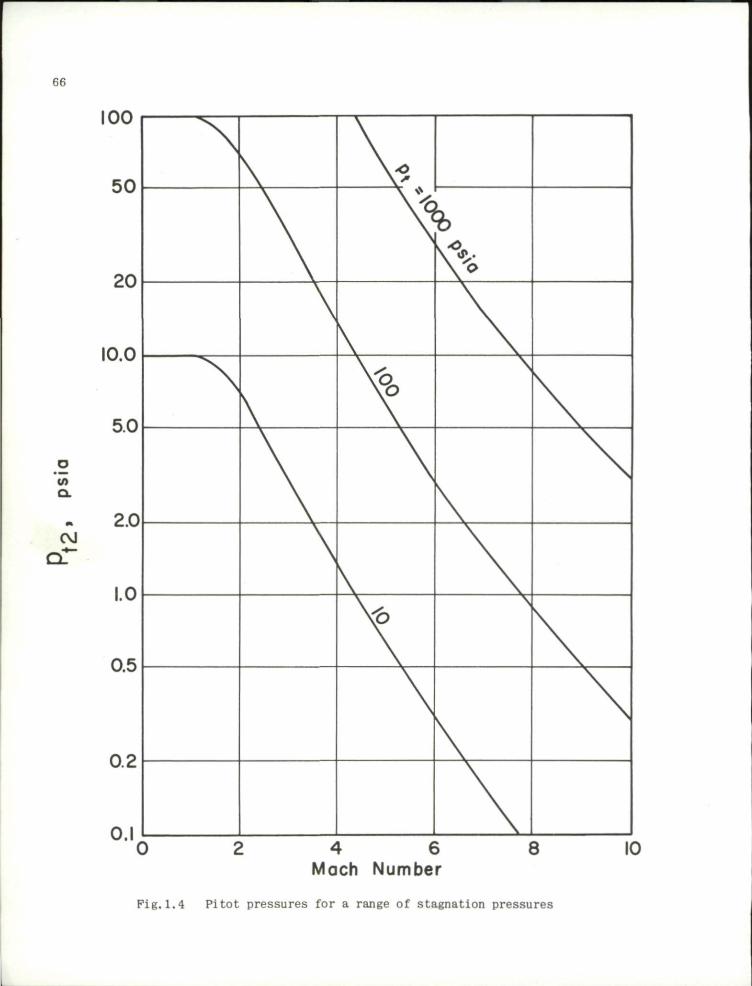
66

100

50

CL

20

10.0

5.0

2.0

1.0

0.5

0.2

0.1

N

\

\b

4 6 Mach Number

8 10

Pig.1.4 Pitot pressures for a range of stagnation pressures

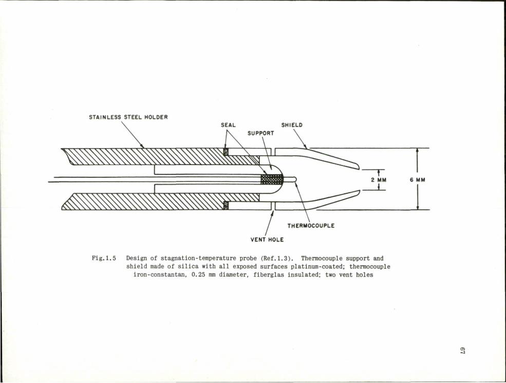
STAINLESS STEEL HOLDER SEAL SHIELD

SUPPORT

VENT HOLE

Fig.1.5 Design of stagnation-temperature probe (Ref.1.3). Thermocouple support and shield made of silica with all exposed surfaces platinum-coated; thermocouple

iron-constantan, 0.25 mm diameter, fiberglas insulated; two vent holes

cn CO

1.00

098

096

T t - T

0.94

0.92

0.90 "— 20 2.2

N U T * * I 0 3

kw

Fig.1.6 Effect of ratio of thermocouple length to diameter for a range of Mach num­bers from 4.90 to 7.60. Nu = Nusselt's number; k and kw = conductivity of

gas and wire. (From Ref.1.3)

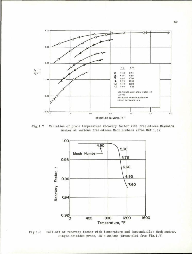
69

T, - T

-DO-

o • V • D

<

7.60

6 95

6 60

5 75

5 30

4 90

1174

1130

1094

1058

I0Z3

628

VENT/ENTRANCE AREA RATIO M5

L / D = I 0

REYNOLDS NUMBER BASED ON

PROBE ENTRANCE 0 .0

REYNOLDS NUMBER «10"

Fig.1.7 Variation of probe temperature recovery factor with free-stream Reynolds number at various free-stream Mach numbers (From Ref.1.3)

1.00

400 800 1200 Temperature, °F

600

Fig.1.8 Pall-off of recovery factor with temperature and (secondarily) Mach number. Single-shielded probe, RN = 20,000 (Cross-plot from Pig.1.7)

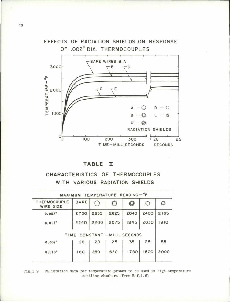
70

EFFECTS OF RADIATION SHIELDS ON RESPONSE

OF .002" DIA. THERMOCOUPLES

3 0 0 0

I Ul

% 2 0 0 0

< cc UJ CL

5 £ 1000

1 1 I I •• I

^ B A R E WIRES 8 A

1

m ^ — \

yy—

/f^\c \E

r ^

<

1

r ]

- f A - O

B - ©

c - © RADIATION

1 L-X t

T T

•

D — O

E — 0

SHIELDS

100 2 0 0 3 0 0

T IME-MILL ISECONDS

2 0

SECONDS

25

TABLE I

CHARACTERISTICS OF THERMOCOUPLES

WITH VARIOUS RADIATION SHIELDS

MAXIMUM TEMPERATURE R E A D I N G - F

THERMOCOUPLE WIRE SIZE

BARE o o o 0.002"

0.013"

0.002"

0.013"

2 7 0 0

2 2 4 0

2655

2 2 0 0

2625

2075

2 0 4 0

1 8 4 5

T I M E CONSTANT - MILLISECONDS

35 20

160

2 0

230

2 5

6 2 0 1 7 5 0

2 4 0 0

2 0 3 0

2 5

1800

2 185

1910

55

2 0 0 0

Pig.1.9 Calibration data for temperature probes to be used in high-temperature sett l ing chambers (From Ref.1.6)

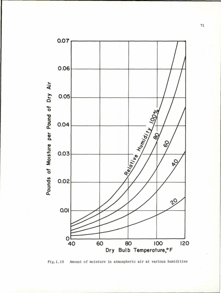
71

0.07

0.06

<

2T 0.05 o

o 0.04

H 0.03

tn T3 0.02

QOI

*v / /

V / / v / /

I . §

i

/ f

&y

40 60 80 100 120 Dry Bulb Temperature,0F

Pig.1.10 Amount of moisture in atmospheric air at various humidities

- J t o

I

8

t l H"

r-rm

rm r -

< p -. r a ­

ft — mm.

c a o

—

1 « I - " . r^

~ — 5 CTJ

09 c -! cr.

T}

ft) V) w c - 1

Q

^ $ 3 | o ZJ

O

o 3 ""m'

o o

- cn

Q

n

ro O

.). o

o

(n O

0)

o

- N I

o

I

o I

Oi o

I ro o

Dew Point Temperature, °F

o o o o OJ

o o Ul O

CD

o - J o

1

o 1

8

\

\ \ ro

i

8

| |

\

\ \

5 5

i v\ V

I

6

<.r

'o

\

\

V o

3**0 ^ f c

~--Osi ^ « 0 "

Nominal Dew Point, Atmospheric Pressure, °F

73

CL I

« CL

i r.Q\

i r.a. i .Ub

CT 1.03

1.00

r . CmaT

20 50 100 200 500 1000 2000 Reynolds Number (Log Scale)

Fig.2,1 Performance of pitot tube at low Reynolds number. Cylindrical tube with orifice diameter = 0.64 tube diameter (A 0.74 orifice produces a slightly

smaller error than shown)

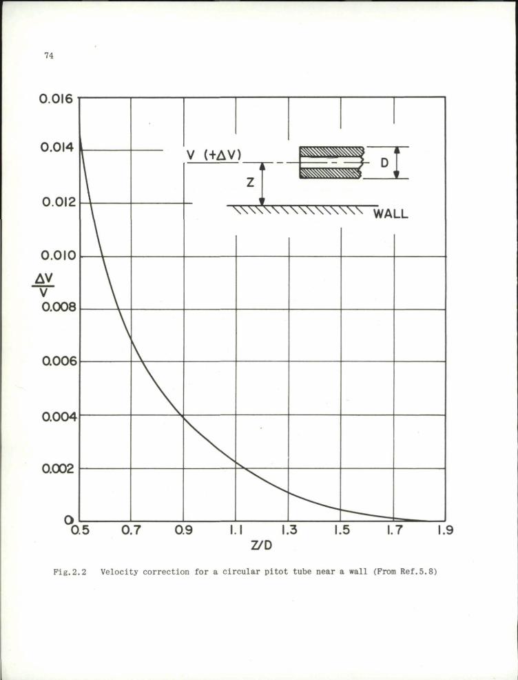
74

u.u ib

0.014

0 012

0.010

AV V 0008

n n n f i U U U D

0.004

0.002

O

V (+AV^ » \ I / U w A

z " V

s \ \ \ \ \ \

sssssssm: ^ D

* W $ S S m ^

vwwv w WA

. i ~

V

LL

0.5 0.7 0.9 I.I 1.3 Z/D

1.5 1.7 1.9

Pig.2.2 Velocity correction for a circular pitot tube near a wall (Prom Ref.5.8)

75

.Static connection

16D B

>|<

Eight holes equally j spaced on periphery

Total-head connection

8D A

Velocity

Fig.2.3 Dimensions of a 'standard' p i t o t - s t a t i c tube

4 8 12 16 20

Static orifice distance from tip base or from stem centerline, diameters. (AB and BC in Pig.2.3).

Fig.2.4 Tip and stem static pressure errors

76

+ 6

+4

2. +2

to

o 1 Cm, c >.

• o

o i—

o5 -t—i

0) CJ

i _

cu

- 2

- 4

- 6

- 8

^ . ^ - - " " " " " • > <

1

^ N

"otal h

-S ta l

s

\ 1

e a d -

ic head

•Dyne

\ \ \ \ \ \

\

A

mic h ead

8 12 Degrees of yaw

16 20

Pig.2.5 Errors in standard pitot-static tube readings produced by yaw

As. 0.02

^yy 0.04 O.OS 0. 2 0.16

M 0.4 o.e

ORIFICE DIAMETER, INCHES

77

FLOW

0.032'^-J d (•— r = d/4

A p . 0.002

r «d

0.011

Ld /S

-0.001

Pig.2.6 Static pressure error due to hole size and lip shape, M = 0.4 to 0.8 (Redrawn from Ref.2.5)

78

£ CO O CD

E

1.00

0.99

I 0 0- 3>

0.98, 0.2 0.4 0.6 0.8

Mach Number 1.0

Pig. 2. 7 Effect of Mach number on temperature recovery ratio of single-shielded probe; pt = 2900 lb/in.

2, Tt = 140°F; tube diameter = 0.12 inch (Redrawn from Ref.2.3)

1.00

T3 CD

CO

o 0)

E

>- 0.99

0.98

• o — $

-30 - 2 0 -10 0 10 20 Yaw Angle, Degrees

30

Pig.2.8 Effect of yaw on temperature recovery factor of single-shielded probe (Same conditions as Fig.2.6) (Redrawn from Ref.2.3)

Fig.2.9 Static pipe installation in a subsonic tunnel (Photo by courtesy of Univer­sity of Washington)

80

Pig.2.10 Spherical type yawmeter

Sphere

Fig.2.11 Spherical yawmeter

81

- 2 . 0

-1.6

-1.2

«?

-0 .8

- 0 . 4

Practice-

-Theory

10 15 20

Angle of yaw, #, degrees

25

Fig.2.12 Calibration curves for the yawmeter in Fig.2.11

82

Fig.2.13 Turbulence sphere and installation (Photo by courtesy of University of Washington)

Four holes evenly spaced

T 22 f

Fig.2.14 Turbulence sphere for a 100 m.p.h. tunnel

83

2.0

1.6 0) o c 0)

1 B 1.2

s 0.8

0.4

n 1.0 1.4 1.8 2.2

Turbulence factor 2.6 3.0

Pig.2.15 Relation between turbulence and turbulence factor

10 e. 11 o tn 0)

• E 4 w" 8 <D

E A3

| 2 c <u

.£= C L

C O

Turbulenc e factor I.. 1.' 1.1

- / f ^ y m

50 90 130 170 Testing velocity, mph (true)

210

Pig.2.16 Chart for estimating most useful diameter for a turbulence sphere

84

• V'i

Fig.2.17 Vortex generators which greatly helped a diffusion problem (Photo by courtesy of University of Wichita)

85

Pig.2.18 Tuft grid for studying large scale fluctuations (Photo by courtesy of University of Wichita)

Differential Pressure Across Yawmeter

o cn

A p Pt-degree

-tl I-1-TS

OO

r—

m 3X3 3

n

< I-1-r t M. a ill o

0 1—'

p 3=

P

C^

8 3

P

^ P

1 s rt 1 DO

^ -n g o 3

33

s

-n n> a> I

CO -^ a> a 3 S Q O 3 "

-z.

3 cr a> ^

O ^1

O 00

o CO

— O

— ^_

ro

OJ

ya

0.012

o.oo8

ft°

1

p.

Jl

mf

0.004

0

-0.004

-0.008

-0.012

e v -50

0.6 0.7 0.8 0.9 1.0 L.l 1.2 1.3 I-1* 1.5 "co

1. 6

Fig.4.1 Difference between plenum chamber static pressure pc and test section static pressure p for a number of wall angles #w in minutes. Nega­tive angles correspond to an expanding section as one proceeds down­

stream (From Ref.4.4)

-I

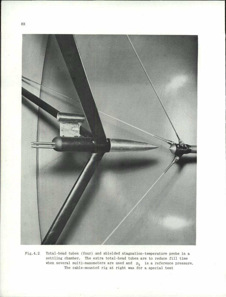
88

Pig.4.2 Total-head tubes (four) and shielded stagnation-temperature probe in a settling chamber. The extra total-head tubes are to reduce fill time when several multi-manometers are used and pt is a reference pressure.

The cable-mounted rig at right was for a special test

Ill - 63 A MACH 1.5 & MACH 2.0 CALIBRATION STATION 22.25

• • B ^ -~

Pig.4.3 Pitot tube in transonic tunnel. Offset is to enable pitot tube to reach into the boundary layer

33

to

CD O

Fig.4.4 Static pipe in the Sandia 12 inch x 12 inch transonic tunnel

Q. \

U.UO

0.04

0 •

• •• • •* •

s

• t

• •

s

• •

« •

• •

4 •

• • .

• •

•

•

\ H » s

mm H « * '

0.5 0.6 0.7 0.8 0.9 1.0 Mach Number

I.I 1.2 1.3 1.4

Pig. 4.5 Plight test data of static pressure probe shown in Fig.5.1; these data read about 0.01 low due to lag

9 2

1.5

1.4

1 .3

1.2

1 .1

SB 1 . 0 •

S

0.9

0.8

0.7

0.6

0.5

OC

trcxn

o o

^ ^

•XJ

^ 3 - _61c ^ O L f f l o - d - Q j

O O Q C

M*^^°^"afcfa'k' ' S ^

xrro

O-CCD-

«,

• ( V C a

cWE^-%

e^^b

c -ax -tpc -o-c d>tio-e -°i5 -%- •%

Croxrxpcre

^a-GcMD-

o n

^ £ x 3>4>£ ° x ^fic j g L r £ 5

<S ^ ih j iJo-G-Q-cx^.

<n

x3La^a|!o-g-o-Q jSkmVS-ip-o &-o

t o

O C e n t e r Line 0 Top Mall

cpogo d

O-O^rCDCn; OCf

t S H ^ - c

<JB -6U3SLO o>C

i3K3 5 K A O - 0 - O - O -q^o -ei-tjo-c OJ-J.

tne ^nsrcOj

-8 -4 8 12 16 20 2** 28 32 36

DISTANCE FROM NOZZLE EXIT, INCHES

Fig.4.6 Calibration plots for a transonic tunnel. The circles are from the static pipe readings; squares are from wall pressure taps (From Ref.4.4)

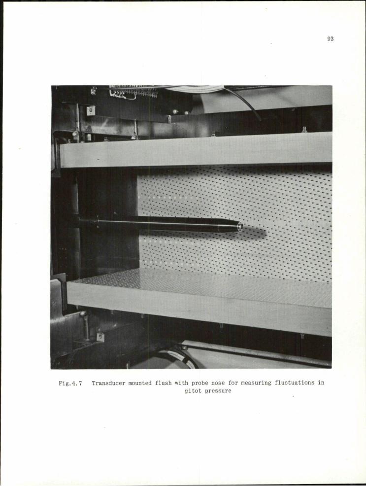
Fig.4.7 Transducer mounted flush with probe nose for measuring fluctuations in pitot pressure

94

o X

£

i.o

0.9

c 0.8 c o

> 0.7 <D

Q

c <D

O 0)

a.

0.6

0.5

O

o o

o ° o

° o o

o

14 15 16 Mean Stagnation Pressure, psia

17

Fig.4.8 Variation of stagnation pressure fluctuations, M = 1.1 (From Ref.4.3)

HOLE PATTERN MUST BE PER­PENDICULAR TO THE TUBE <j SO

THAT THE PLANE OF THE HOLE ( j

WILL SHOW NO MORE THAN .003 TI.R

8°(REF)

i.ooi ,—.117 DIA.

rV <!>

3.65 1.840

V l v r DRILL NO. 56-0465 DIA 24 HOLES EXTERNAL 8 INTERNAL SURFACES MUST BE BURR FREE EXTERNAL EDGES MUST BE SHARP

.281 DIA-<£> tooi

6 , <JV249°DiA

U ^ fl 1° TAPER (REF)

.250 -J 125

1.50

7 0 0 ^ - - 4.650

7.190 (REF)

i r toio

.171 DIA

-.223 DIA.

A

1.

•

* \ '~ 093

<j) THESE DIAMETERS MUST BE CONCENTRIC TO .002 TI.R.

-.020 DIA

Pig.5.1 Dimensions of supersonic static pressure probe (From Ref.5.2)

to

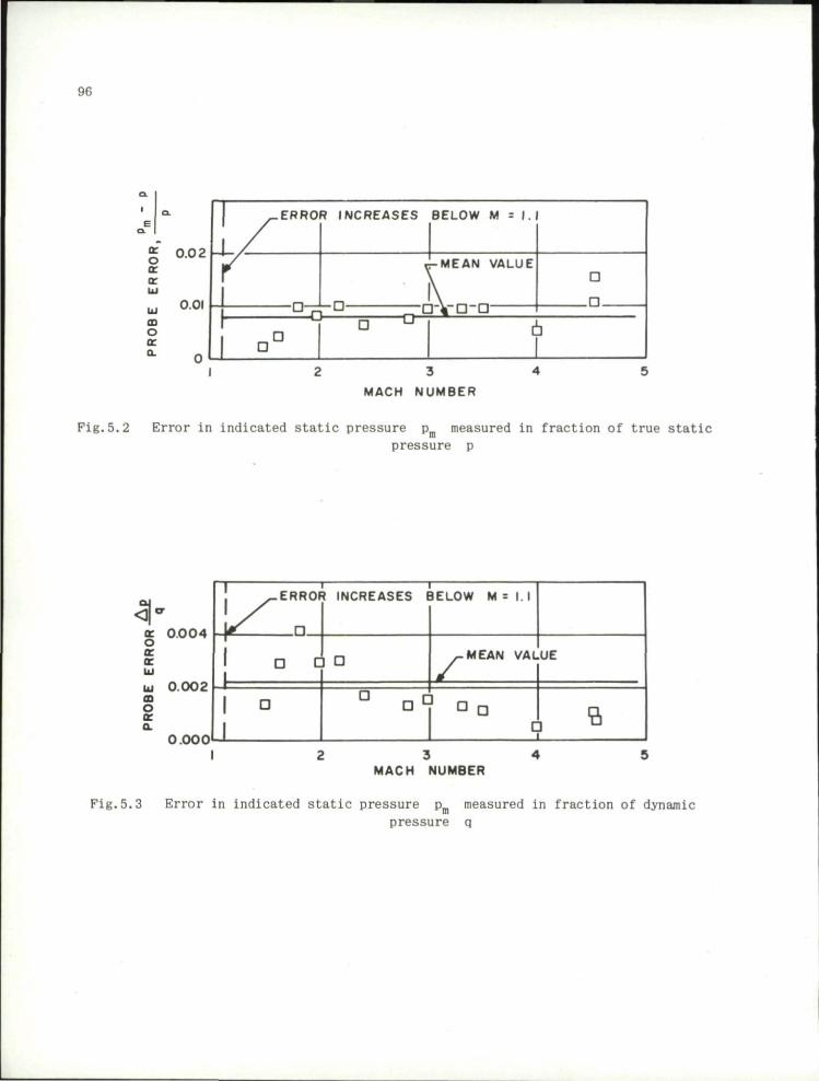
on

ERROR INCREASES BELOW M = I.I

MEAN VALUE

TJ

K Q V D - Q

D

. D .

MACH NUMBER

Fig.5 .2 Error in indicated s t a t i c pressure pm measured in fract ion of t rue s t a t i c pressure p

* a. 0.004 o or

UJ 0.002 a. o a:

0.000

I 1 .ERROR INCREASES BELOW M = 1.1

D • ° z MEAN VALUE

o° a a a

_ i _

s i

MACH NUMBER

Fig.5.3 Error in indicated static pressure pm measured in fraction of dynamic pressure q

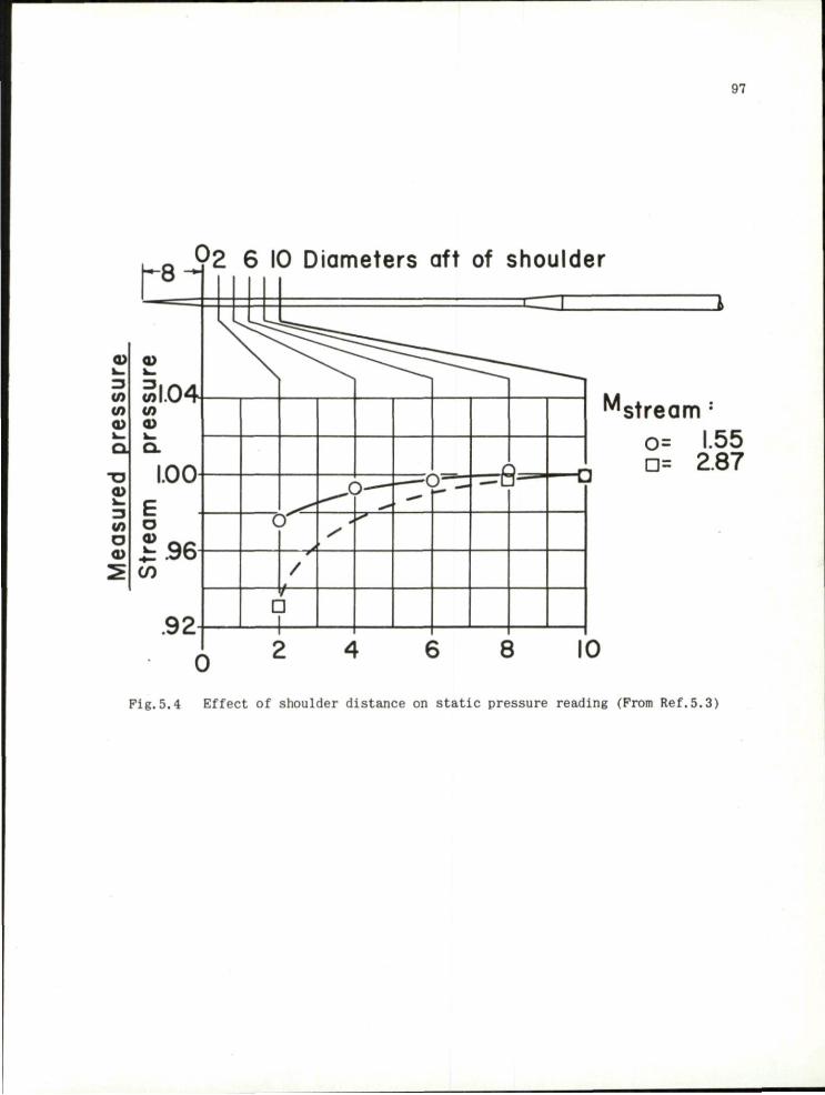
97

J?2 6 10 Diameters aft of shoulder F 8 1

a> J V .

</> V) a>

a o. 0) ) J W

V)

a

M stream :

o= I.55 n= 2.87

Fig.5.4 Effect of shoulder distance on static pressure reading (From Ref.5.3)

98

-0.04

<

c o • H

+•>

•H > 0) Q

U OS S

-0 08

-0.12

-0.16

-0.20

—6 Reynolds Number Per Inch x 10~

0.1 0.2 0.3 0.

-0.24

Fig.5.5 Variation of centerline Mach number with Reynolds number, 40 inch tunnel (From Ref.5.10)

£.*t

2.0

1.6

E 3 z 1.2 c u o 5 " 0.8

0.4

0

my b^ 1 o

JZ

1 1 1 t

Tunne Side Wal l -

Axis -

-Contoui -ed Wall

24 22 20 18 16 14 12 10 8 6

Distance Upstream From Nozzle Exit, Inches

Fig.5.6 Calibration data from M = 2.0 nozzle (Redrawn from Ref.5.4)

s

100

Approximate Edge of Boundary Layer

o <

c o

- 6 - 4 - 2 0 2 4 6 Distance to Right of Observer Looking Upstream,

Inches

Pig.5.7 Contour plot of an M = 3.0 nozzle (Redrawn from Ref.5.4)

3 U

80

. A

ng

le,

De

gre

i

5 3

> o

mt JC u o t% 50

40

^

^ ' »

^

Vx1 \ 1

• & - <

f /

v.

TJ 7 *>

^ \ \ 1

8 12 16 20 Deflection Angle, Degrees

24

Fig.5.8 Wave angles for a range of wedge semi-angles

101

Pig.5.9 Wedge dimensions and set-up for angularity measurements (From Ref.5.9)

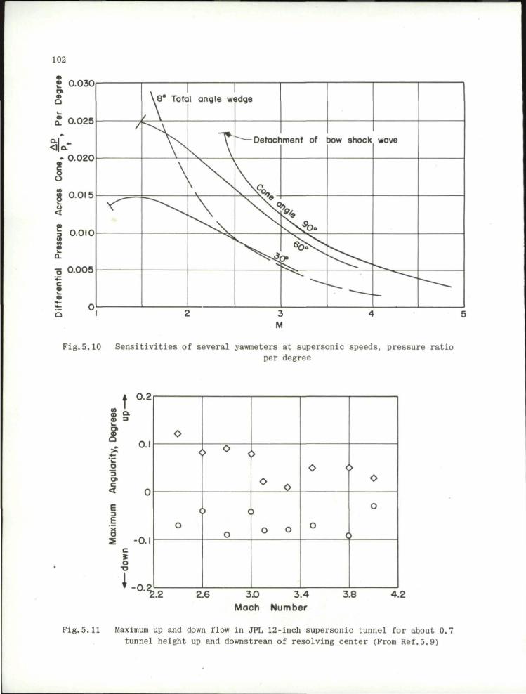
102

Pig.5.10 Sensitivities of several yawmeters at supersonic speeds, pressure ratio per degree

0.2

0.1

o

E E X O 2 -0.1

c i o TJ

l-o. £

o

T ^ r o i

y ^ . L_! I I ° 0 o o ° r i

2.6 3.0 3.4 Mach Number

3.8 4.2

Pig.5.11 Maximum up and down flow in JPL 12-inch supersonic tunnel for about 0.7 tunnel height up and downstream of resolving center (Prom Ref.5.9)

O r i f i c e Diam 0.050 Four S t a t i c

O r i f i c e s 0.035 Diam

Fig.5.12 Calibration rake (Prom Ref.5.10) s

i.ssT" 24.07"

30 Equally Spaced Thermocouples 2.164" Dia.

0.75 Dia

2

Fig.5.13 Dimensions of JPL transition cone (Prom Ref.5.12)

o?

o •p o a

>3.

o o o fj

ts U

*J t u

s I

.90

.80

.06

.04

Lam Inar z 3116 6 '

/

V /

1 1 1 Turbulent zone

i- Transition length » 8. 5 in.

i 6 8 10 Distance along cone, in.

12 14 16

Fig.5.14 Typical determination of transition Reynolds number. Free-stream Reynolds number per foot, 4.31 x 106; transition Reynolds number 3.055 x 106

(Prom Ref. 5.11)

105

Mach Number

Fig.5.15 Transition Reynolds number on 5° and 10° cones as measured at several facilities (From Ref.5.13)

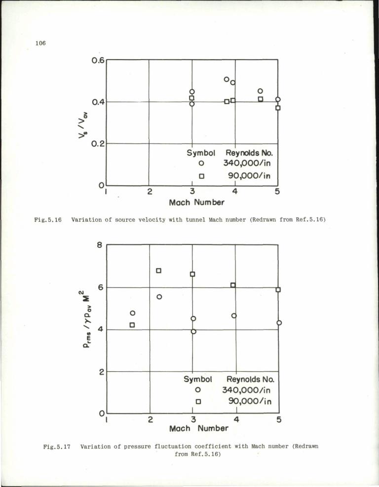
106

0.6

0.4

>

0.2

-oc-o

i

Symbol Reynolds No. O 340,000/in

D 90,000/ in

1 2 3 4 5 Mach Number

Pig.5.16 Variation of source velocity with tunnel Mach number (Redrawn from Ref.5.16)

8

CJ

> o

Q.

E

o D

•

O

c

<

<

i

)

c

c

p

Symbol O

a i

u

()

Reynolds No. 3 4 0 , 0 0 0 / i n

9 0 , 0 0 0 / i n 1

3 4 Mach Number

Fig.5.17 Variation of pressure fluctuation coefficient with Mach number (Redrawn from Ref.5.16)

Pig.5.18 Noise emanating from turbulent boundary layer on a missile model. M = 3.5; RN = 2 x lOVinch. Note the diminution of wavelet strength as the distance

from the source is increased (From Fig.4(y) of Ref.5.20)

108

12.0

10.0

£ 8.0

E 3

S 6.0 5

4.0

2.0

Stagnation PS

Pressure IA ^Sso.o

^^ •100 .0

-e^ -6000 ^Ibooo

500 700 900 1100 1300 1500 Stagnation Temperature,°R

1700 1900

Fig. 6.1 Mach number for equilibrium condensation of air (Prom Ref.6.1)

109

M

lOO-ZOo'F.

St

Po

Tft

•*- MO MIR CONDENSATION

ABOVE PRE EXRMPLES or CLOSE-COUPLED PITOT TUBE RND TRANSDUCER TRBCE5 ON M O S L E Y PLOTTER

Fig.6.2 Methods of detecting liquefaction in a hypersonic tunnel (From Ref.6.2)

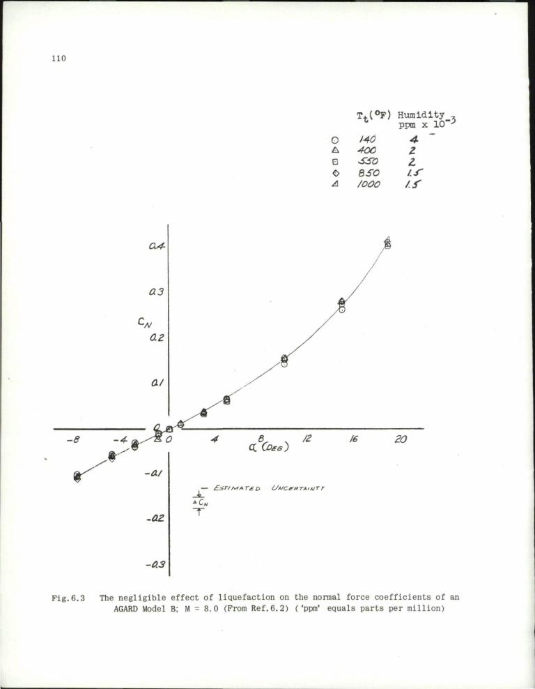
no

0 A E 0 at.

T t ( ° F )

140 40C .SSO 8SO /OOO

Humidity , ppm x lO"-3

-4 Z z /mmT

f f

- 8 - 4 -

Mr - A /

-az

-0 .3

fl, . /2

— £sr/fa**r£CJ UfJceRTAiurr

Fig.6.3 The negligible effect of liquefaction on the normal force coefficients of an AGARD Model B; M = 8.0 (From Ref.6.2) ('ppm' equals parts per million)

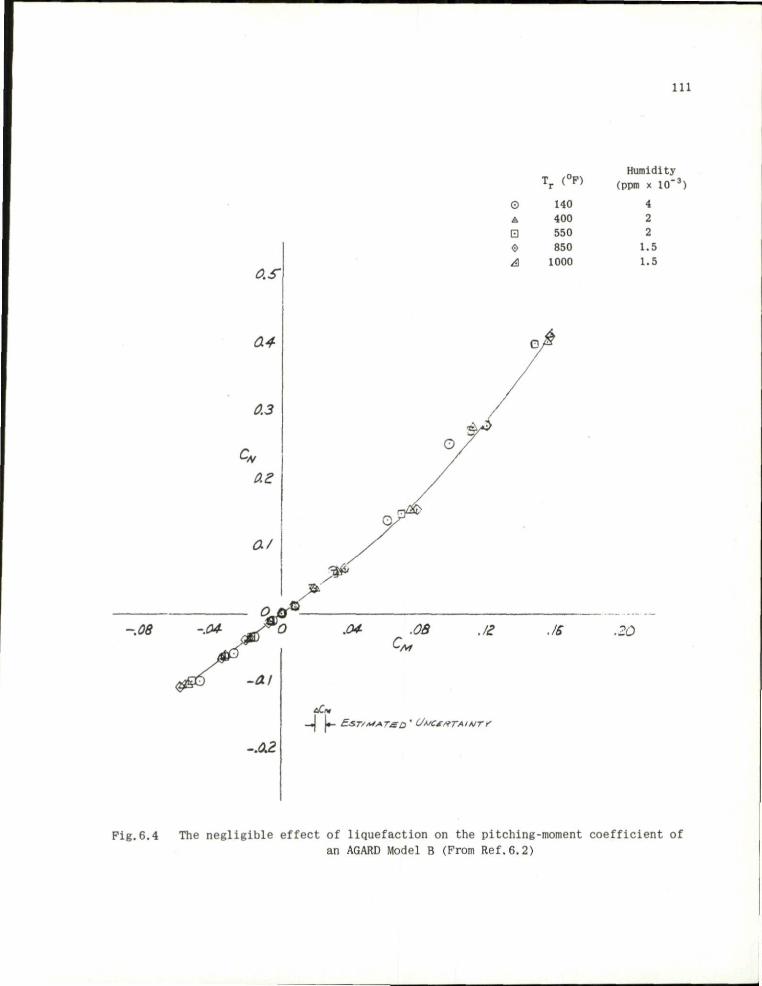
I l l

Humidity

0 A

• 0 A

T r (°P)

140 400 550 850

1000

(ppm x 10"3)

4 2 2

1.5 1.5

-.0.2

www

.20

Pig.6.4 The negligible effect of liquefaction on the pitching-moment coefficient of an AGARD Model B (From Ref.6.2)

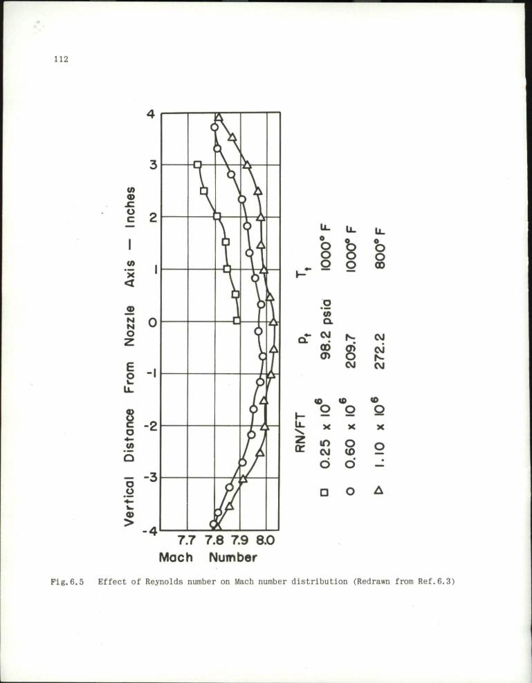
112

<m Q O

o o o 00

*• Q.

\— U-•^ z or

v> a.

CM

cn

<D o ~~ X

m CvJ

o

i ^

s CVJ

<0 O X

O

O

CO CVJ

CM

<0 O X

O

•

7.7 7.8 7.9 8.0 Mach Number

Pig.6.5 Effect of Reynolds number on Mach number distribution (Redrawn from Ref. 6.3)

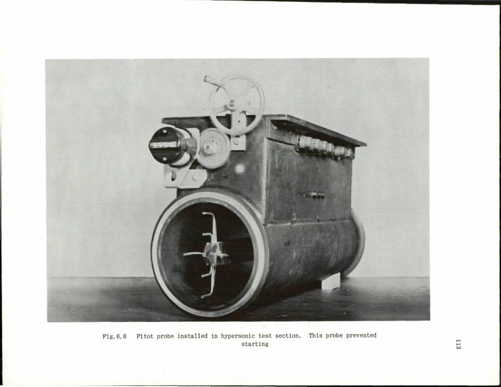
Fig.6.6 Pitot probe installed in hypersonic test section. This probe prevented starting

u

0.7 -

0.6 -

0.5 -

0.4

y*F or 0.3

0.2

0.1

Limit Based on Entropy Change One Dimensional Normal Shock Theory

<o3

4

9 .o

Open Solid Flagged

Tunnel Start Marginal

Tunnel Started Tunnel Blocked

1 •

0 D O Cm

lm

A

1 2 - i n . 1 2 - i n . 2 0 - i n . 1 2 - i n . 5 0 - i n . 1 6 - i n .

Tunnel

s q , s u p e r s o n i c , AEDC s q , s u p e r s o n i c , JPL

s u p e r s o n i c , JPL sq , h y p e r s o n i c , AEDC diam, h y p e r s o n i c , AEDC diam, h y p e r v e l o c i t y , AEDC

8 10 Mach Number

12 14 16 18 20

Fig. 6.7 Summary of data on the effect of model size and shape on starting; d is model diameter, A is test section geometric area, and A_ is test section geometric

area less the boundary layer displacement thickness area (From Ref.6.7)

T O D , - . D

3" 2"—1

* ' 0 <

i 4" 4

4-0 .025"d iamefer holes

Fig.6.8 Static pressure rake with small error

[, Vacuum

AP

r i E

Y 1

a B

Mercury

Fig.6.9 Diagram of low-pressure manometer Fig.6.10 Elements of McLeod gage

117

1000 0 0 20 30 40 50 60

AXIAL DISTANCE FROM THROAT-INCHES NOZZLE THROAT

Pig.6.11 Measurements of the stagnation temperature along the axis of the settling chamber of a 6 inch x 6 inch wind tunnel; the solid circles are from measurements in the test section, not the throat as shown (Ref.6.6)

u 0)

~ p. m. 0)

J 3 +J

j m .

m •M

a. - V (N «JJ

a

V l i -ai a .mm

n * J

a M •M

a • ^

I.I

_

•jjj tHs, S s ^ s

; : : : : : : : : : : S J ; : : S ; : ; ; : : : : : : : : : : : : 5 s v _

S " Q S ^ fc

L 5 * . 1 1

> 5 5 5

C T"^, ^ _ S * r s . _ M - .

^ ___ 5 Q 5

S ^ \^ ^ k

j .

_ „ _ v __\

. __ s t _ _ 5S 7 ^

0 7; = l 0 0 o R

6

ure, / / • 1000 n | | | 1 1 | I I I | 1 t - H - P " = = = = = = = = = = = = = = = = = = = = = = = = = = = = = =

I ! 2 0 0 0 ° R

: 3 0 0 0 ' R : : : : : : :

= W = -I—i—1—1— = = = = = = = =

4 5 6 Moch number, M,

10

Fig.6.12 Effect of caloric imperfections on total-pressure ratio across a normal

shock wave (From Ref.1,2)

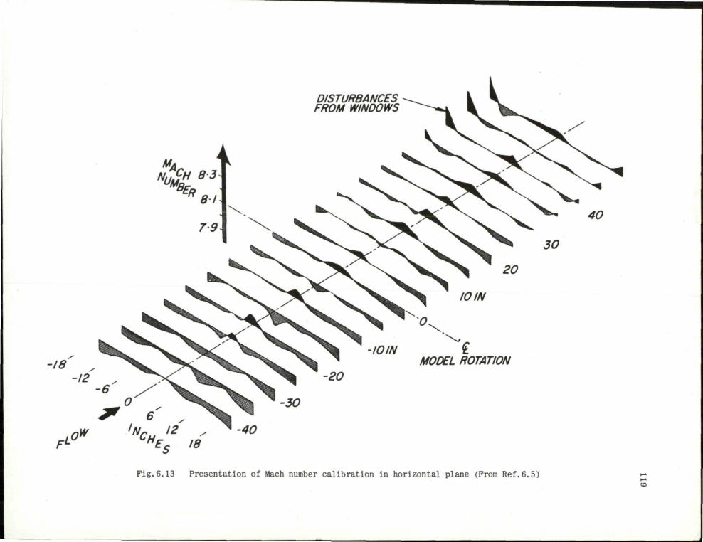
N U M " 8 3

DISTURBANCES FROM WINDOWS

MODEL ROTATION

Pig. 6.13 Presentation of Mach number calibration in horizontal plane (From Ref.6.5)

to O

Fig.6.14 Shadowgraph of flow angularity probe (From Ref.6.5)

121

4

•a

• 3

O

o c

0 s*

<D 1 N '

8 z

1 ° u_ <D O 1 C ' o to o

tm.

Ve

rtic

al

OJ

r

4

o v^

_J

i

i

1 f\ t \J

o

1 D

^ y r x

1/1 ,

-1.0 1.0

Flow Angle, Degrees

Pig.6.15 Presentation of flow angularity data, M - 7.2 (Redrawn from Ref.6.3)

122

TRANSITION IN WAKE (LAMINAR FLOW)

x i -o z UJ

z

(/)

TRANSITION ON MODEL • (TURBULENT FLOW)

REYNOLDS NUMBER

Fig .7 .1 Typical curve of c r i t i c a l s t ing length vs. Reynolds number (From Ref.7.2)

RN,

Fig.7.2 The effect of Reynolds number on critical sting length (From Refs.7.2 and 7.6)

123

0.45

0.40

0.35

0.30

1 \ m .

^ ^ J T

0.2 0.4

d/D

0.6

Fig.7.3 Effect of sting to model diameter ratio on base pressure of an ogive-cylinder model; RN = 15 x 10*. turbulent boundary layer, M = 2.97

(Redrawn from Ref.7.7)

. Circular-ore profile. Maximum diom. -r= t / c * 0 . i 0 *v,

10 0.0997*.

Pig.7.4 General configuration of RM-10 (AGARD Model A) research model (From Ref.7.11)

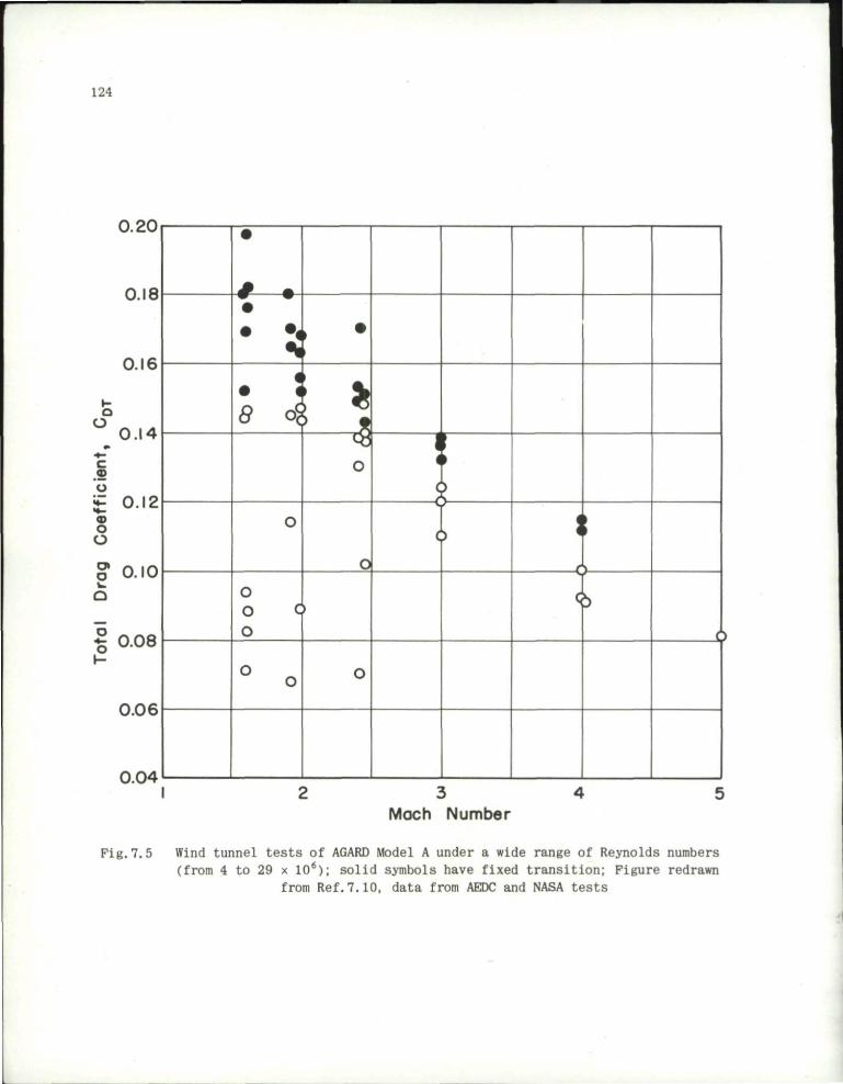
124

0.20

0.18 4-

0.16

O

5

0.14

u £ 0.12 8 01 0.10 2

I 0.08

8 d?

o o o

4-

I 4

-0

0.06

0.04

Mach Number

Fig.7.5 Wind tunnel tests of AGARD Model A under a wide range of Reynolds numbers (from 4 to 29 x 106); solid symbols have fixed transition; Figure redrawn

from Ref.7.10, data from AEDC and NASA tests

125

0.04

0.03 -CL,

R - 8 x 10 O Tunnel E-l (Ref. 7.12)

D Tunnel E-l (Ref.7.13)

• Tunnel A

np

gg •M

a 0)

9 o u gj a

s

0.05

0.04 -

0.03

0.02

0.01 -

D,T

D,b

L i f t Cu rve S l o p * , N e u t r a l P o i n t L o c a t i o n , and D rag C o e f f i c i e n t s (or A G A R D C a l i b r a t i o n Mode l B

Fig.7.6 Results from tests of the AGARD Model B in several wind tunnels; CLa is the slope of the lift curve, CD b the base drag coefficient; CD T the total drag coefficient; x the distance from the nose to the neutral point in body

diameters (From Ref.5.10)

Location of transition strips when installed

to mT3

Pig.7.7 Drawing of AGARD calibration Model B. Equation of nose contour:

r = — 3

l/x\2 l/xx3

9\d/ 54\d ; all dimensions are in inches unless

otherwise noted; airfoil 4% circular arc (From NACA TN 3300)

127

.20

CDrj - 1 0

,10

'°B

8

o

S C D P

.10

.20

.10

8 16 24 32 Reynolds Number, R

40x10*

Fig. 7.8 Comparison of AGARD Model A data from tests in several tunnels; M - 1.6, fins off (From Ref.7.11)

128

Fig.7.9 Boeing Aircraft Corporation hypersonic research force model

UJ UJ

cc <mO

UJ o

or UJ CL

0 .025

0 . 0 2 0

0.015

o

0.010

0 . 0 0 5

FACILITY M R N / F T X I O ' 6

o AEDC E-l 2.50 2 . 9 6 o AEDC E-l 3.49 4 . 2 5 o AEDC E-l 4.98 2 . 7 4 a NSL, MIT 2.51 2 . 8 3 • NSL, MIT 3.56 4. 14 A BOEING 6.07 12 .60

4 5 Mach Number

0 . 0 2 5

o Q

O 0 .020

o mm 0 . 0 1 5 N

£ o.oio

o o

a> o

0 . 0 0 5

o o 0

D

D

A

FACILITY

AEDC E-l AEDC E-l AEDC E-l N S L , MIT NSL , M I T BOEING

M

2 .50 3.49 4 .98 2.51 3,56 6 .07

• / RN/FTx 10

2 . 9 6 4 . 2 5 2 . 7 4 2. 83 4. 14

12 .60

>T

8

Mach Number

Fig.7.10 Comparison of wind-tunnel tests of Boeing hypersonic glider model: slope of normal force

curve (From Ref.7.14)

Pig.7.11 Comparison of wind-tunnel tests of Boeing hypersonic glider model: drag at zero lift

(From Ref. 7.14) to

o

o

o o

o

tv Q. o

co

1.4

1.2

1.0

0 . 8

o o 0 . 6 a.

0 . 4

0 .2

FACILITY M R N / F T X I O " 6

AEDC E-l 2.50 2 . 9 6 AEDC E-l 3.49 4 . 2 5 AEDC E-l 4 .98 2 .74 N S L , M I T 2.51 2 . 8 3 N S L , M I T 3.56 4 . 1 4 BOEING 6 .07 12 .60

00

o

0.05

a>* - 0 . 0 4

o

c 0J E o E i

cn c

•0 .03

•0 .02

•s -o .o i a> Q. O

CO

FACILITY M R N / F T X I 0 ' 6

o AEDC E-l 2 .50 2 . 9 6 0 AEDC E-l 3,49 4 . 2 5 0 AEDC E-l 4 .98 2 . 7 4 a NSL, MIT 2.51 2 . 8 3 D NSL, MIT 3 .56 4 . 14 A BOEING 6 . 0 7 1 2 . 6 0

D

O

D

O

o

4 5 6 Mach Number

4 5

Mach Number

Fig.7.12 Comparison of wind-tunnel tests of Boeing hypersonic glider model: slope of drag polar

(Prom Ref. 7.14)

Fig.7.13 Comparison of wind-tunnel tests of Boeing hypersonic glider model: slope of pitching-

moment curve (From Ref.7.14)

E-

H o H

o o o

1.6 TUT Mach Number, M

Fig. 7.14 Comparison of wind-tunnel and f l ight drag data for AGARD Model A (From Ref. 7.11)

DISTRIBUTION

Copies of AGARD publications may be obtained in the various countries at the addresses given below.

On peut se procurer des exeraplaires des publications de 1'AGARD aux adresses suivantes.

BELGIUM BELGIQUE

Centre National d' Etudes et de Recherches Aeronautiques 11, rue d'Egmont, Bruxelles

CANADA Director of Scientific Information Service Defense Research Board Department of National Defense 'A' Building, Ottawa, Ontario

DENMARK DANEMARK

Military Research Board Defense Staff Kastellet, Copenhagen 0

FRANCE O.N.E.R.A. (Direction) 25, Avenue de la Division Leclerc Chatillon-sous-Bagneux (Seine)

GERMANY ALLEMAGNE

Wissenschaftliche Gesellschaft fur Luftfahrt Zentralstelle der Luftfahrtdokumentation Munchen 64, Flughafen Attn: Dr. H.J. Rautenberg

GREECE GRECE

Greek National Defense General Staff B. MEO Athens

ICELAND ISLANDE

Director of Aviation c/o Flugrad Reykjavik

ITALY ITALIE

Ufficio del Generale Ispettore del Genio Aeronautico Ministero Difesa Aeronautica Roma

LUXEMBURG LUXEMBOURG

Obtainable through Belgium

NETHERLANDS PAYS BAS

Netherlands Delegation to AGARD Michiel de Ruyterweg 10 Delft

NORWAY

NORVEGE

Mr. 0. Blichner Norwegian Defence Research Establishment

Kjeller per Lillestrom

PORTUGAL Col. J.A. de Almeida Viama (Delegado Nacional do 'AGARD') Direcc,ao do Servico de Material da F.A. Rua da Escola Politecnica, 42 Lisboa

TURKEY TURQUIE

Ministry of National Defence

Ankara Attn. AGARD National Delegate

UNITED KINGDOM

ROYAUME UNI

Ministry of Aviation

T.I.L., Room 009A

First Avenue House

High Holborn

London W.C.I

UNITED STATES ETATS UN IS

National Aeronautics and Space Administration (NASA) 1520 H Street. N.W.

Washington 25, D.C.

* Printed by Technical Editing and Refiroduction Ltd

95 Great Portland S t . London, V. l .