against poverty s c · pdf file1578 quarterly journal of economics poverty lines than poor...
TRANSCRIPT

THE DEVELOPING WORLD IS POORER THAN WETHOUGHT, BUT NO LESS SUCCESSFUL IN THE FIGHT
AGAINST POVERTY∗
SHAOHUA CHEN AND MARTIN RAVALLION
A new data set on national poverty lines is combined with new price dataand almost 700 household surveys to estimate absolute poverty measures for thedeveloping world. We find that 25% of the population lived in poverty in 2005, asjudged by what “poverty” typically means in the world’s poorest countries. Thisis higher than past estimates. Substantial overall progress is still indicated—thecorresponding poverty rate was 52% in 1981—but progress was very uneven acrossregions. The trends over time and regional profile are robust to various changesin methodology, though precise counts are more sensitive.
I. INTRODUCTION
When the extent of poverty in a given country is assessed,a common (real) poverty line is typically used for all citizenswithin that country, such that two people with the same standardof living—measured in terms of current purchasing power overcommodities—are treated the same way in that both are eitherpoor or not poor. Similarly, for the purpose of measuring povertyin the world as a whole, a common standard is typically appliedacross countries. This assumes that a person’s poverty status de-pends on his or her own command over commodities, and not onwhere he or she lives independently of that.1
In choosing a poverty line for a given country one naturallylooks for a line that is considered appropriate for that country,while acknowledging that rich countries tend to have higher real
∗A great many colleagues at the World Bank helped us in obtaining the nec-essary data for this paper and answered our many questions. An important ac-knowledgement goes to the staff of over 100 governmental statistics offices whocollected the primary household and price survey data. Our thanks go to PremSangraula, Yan Bai, Xiaoyang Li, and Qinghua Zhao for their invaluable help insetting up the data sets we use here. The Bank’s Development Data Group helpedus with our many questions concerning the 2005 ICP and other data issues; we areparticularly grateful to Yuri Dikhanov and Olivier Dupriez. We have also benefitedfrom the comments of Francois Bourguignon, Gaurav Datt, Angus Deaton, Mas-soud Karshenas, Aart Kraay, Peter Lanjouw, Rinku Murgai, Ana Revenga, LuisServen, Merrell Tuck, Dominique van de Walle, Kavita Watsa, and the journal’seditors, Robert Barro and Larry Katz, and anonymous referees. We are especiallygrateful to Angus Deaton, whose comments prompted us to provide a more com-plete explanation of why we obtain a higher global poverty count with the newdata. These are our views and should not be attributed to the World Bank or anyaffiliated organization. [email protected]; [email protected].
1. For further discussion of this assumption, see Ravallion (2008b) and Raval-lion and Chen (2010).C© 2010 by the President and Fellows of Harvard College and the Massachusetts Institute ofTechnology.The Quarterly Journal of Economics, November 2010
1577

1578 QUARTERLY JOURNAL OF ECONOMICS
poverty lines than poor ones. (Goods that are luxuries in rural In-dia, say, are considered absolute necessities in the United States.)There must, however, be some lower bound, because the cost of anutritionally adequate diet (and even of social needs) cannot fallto zero. Focusing on that lower bound for the purpose of measur-ing poverty in the world as a whole gives the resulting povertymeasure a salience in characterizing “extreme poverty,” thoughhigher lines are also needed to obtain a complete picture of thedistribution of levels of living.
This reasoning led Ravallion, Datt, and van de Walle (RDV)(1991)—in background research for the 1990 World DevelopmentReport (World Bank 1990)—to propose two international lines: thelower one was the predicted line for the poorest country and thehigher one was a more typical line amongst low-income countries.The latter became known as the “$1-a-day” line. In 2004, aboutone in five people in the developing world—close to one billionpeople—were poor by this standard (Chen and Ravallion 2007).
This paper reports on the most extensive revision yet of theWorld Bank’s estimates of poverty measures for the developingworld.2 In the light of a great deal of new data, the paper estimatesthe global poverty count for 2005 and updates all past estimatesback to 1981.
New data from three sources make the need for this revisioncompelling. The first is the 2005 International Comparison Pro-gram (ICP). The price surveys done by the ICP have been the maindata source for estimating PPPs, which serve the important role oflocating the residents of each country in the “global” distribution.Prior to the present paper, our most recent global poverty mea-sures had been anchored to the 1993 round of the ICP. A betterfunded round of the ICP in 2005, managed by the World Bank,took considerable effort to improve the price surveys, includingdeveloping clearer product descriptions. A concern about the 1993and prior ICP rounds was a lack of clear standards in defining in-ternationally comparable commodities. This is a serious concernin comparing the cost of living between poor countries and richones, given that there is likely to be an economic gradient in thequality of commodities consumed and (relatively homogeneous)“name brands” are less common in poor countries. Without strictstandards in defining the products to be priced, there is a risk
2. By the “developing world” we mean all low- and middle-income countries—essentially the Part 2 member countries of the World Bank.

POVERTY IN THE DEVELOPING WORLD 1579
that one will underestimate the cost of living in poor countriesby confusing quality differences with price differences. The newICP data imply some dramatic revisions to past estimates, consis-tent with the view that the old ICP data had underestimated thecost-of-living in poor countries (World Bank 2008b).
The second data source is a new compilation of poverty lines.The original “$1-a-day” line was based on a compilation of nationallines for only 22 developing countries, mostly from academic stud-ies in the 1980s. Although this was the best that could be doneat the time, the sample was hardly representative of developingcountries even in the 1980s. Since then, national poverty lineshave been developed for many other countries. Based on a newcompilation of national lines for 75 developing countries providedby Ravallion, Chen, and Sangraula (2009), this paper implementsupdated international poverty lines, in the spirit of the aim of theoriginal $1-a-day line, namely to measure global poverty by thestandards of the poorest countries.
The third data source is the large number of new householdsurveys now available. We draw on 675 surveys, spanning 115countries and 1979–2006. (In contrast, the original RDV estimatesused 22 surveys, one per country; Chen and Ravallion [2004] used450 surveys.) Each of our international poverty lines at PPP isconverted to local currencies in 2005 and then is converted to theprices prevailing at the time of the relevant household survey us-ing the best available Consumer Price Index (CPI). (Equivalently,the survey data on household consumption or income for the sur-vey year are expressed in the prices of the ICP base year, and thenconverted to PPP dollars.) Then the poverty rate is calculated fromthat survey. All intertemporal comparisons are real, as assessedusing the country-specific CPI. We make estimates at three-yearintervals over the years 1981–2005. Interpolation/extrapolationmethods are used to line up the survey-based estimates with thesereference years, including 2005. We also present a new method ofmixing survey data with national accounts (NAS) data to try toreduce survey-comparability problems. For this purpose, we treatthe national accounts data on consumption as the data for predict-ing a Bayesian prior for the survey mean and the actual survey asthe new information. Under log-normality with a common vari-ance, the mixed posterior estimator is the geometric mean of thesurvey mean and its predicted value based on the NAS.
These new data call for an upward revision of our past es-timates of the extent of poverty in the world, judged by the
1580 QUARTERLY JOURNAL OF ECONOMICS
standards of the world’s poorest countries. The new PPPs im-ply that the cost of living in poor countries is higher than wasthought, implying greater poverty at any given poverty line. Work-ing against this effect, the new PPPs also imply a downward revi-sion of the international value of the national poverty lines in thepoorest countries. On top of this, we also find that an upward re-vision to the national poverty lines is called for, largely reflectingsample biases in the original data set used by RDV. The balance ofthese data revisions implies a higher count of global poverty by thestandards of the world’s poorest countries. However, we find thatthe poverty profile across regions and the overall rate of progressagainst absolute poverty are fairly robust to these changes, andto other variations on our methodology.
II. PURCHASING POWER PARITY EXCHANGE RATES
International economic comparisons have long recognizedthat market exchange rates are deceptive, given that some com-modities are not traded internationally; these include services butalso many goods, including some food staples. Furthermore, thereis likely to be a systematic effect, stemming from the fact that lowreal wages in developing countries entail that nontraded goodstend to be relatively cheap. In the literature, this is known asthe “Balassa–Samuelson effect” (Balassa 1964; Samuelson 1964),which is the most widely accepted theoretical explanation for anempirical finding known as the “Penn effect”—that richer coun-tries tend to have higher price indices, as given by the ratios oftheir PPPs to the market exchange rate.3 Thus GDP comparisonsbased on market exchange rates tend to understate the real in-comes of developing countries. Similarly, market exchange ratesoverstate the extent of poverty in the world when judged relativeto a given US$ poverty line. Global economic measurement, in-cluding poverty measurement, has relied instead on PPPs, whichgive conversion rates for a given currency with the aim of en-suring parity in terms of purchasing power over commodities,both internationally traded and nontraded. Here we only pointto some salient features of the new PPPs relevant to measur-ing poverty in the developing world.4 We focus on the PPP for
3. The term “Penn effect” stems from the Penn World Tables (Summers andHeston 1991).
4. Broader discussions of PPP methodology can be found in Ackland, Dowrick,and Freyens (2007), World Bank (2008b), Deaton and Heston (2010), and Ravallion(2010).
POVERTY IN THE DEVELOPING WORLD 1581
individual consumption, which we use later in constructing ourglobal poverty measures.5
The 2005 ICP is the most complete and thorough assessmentto date of how the cost of living varies across the world, with146 countries participating.6 The world was divided into six re-gions (Africa, Asia–Pacific, Commonwealth of Independent States,South America, Western Asia, and Eurosat–OECD) with differ-ent product lists for each. The ICP collected primary data on theprices for 600–1,000 (depending on the region) goods and servicesgrouped under 155 “basic headings” corresponding to the expen-diture categories in the national accounts; 110 of these relate tohousehold consumption. The price surveys covered a large sam-ple of outlets in each country and were done by the governmentstatistics offices in each country, under supervision from regionaland World Bank authorities.
The price surveys for the 2005 ICP were done on a more sci-entific basis than prior rounds. Following the recommendations ofthe Ryten Report (United Nations 1998), stricter standards wereused in defining internationally comparable qualities of the goods.Region-specific detailed product lists and descriptions were de-veloped, involving extensive collaboration amongst the countriesand the relevant regional ICP offices. Not having these detailedproduct descriptions, it is likely that the 1993 ICP used lowerqualities of goods in poor countries than would have been foundin (say) the U.S. market.7 This is consistent with the findings ofRavallion, Chen, and Sangraula (RCS) (2009) suggesting that asizable underestimation of the 1993 PPP is implied by the 2005data. Furthermore, the extent of this underestimation tends to begreater for poorer countries.
The regional PPP estimates were linked through a commonset of global prices collected in 18 countries spanning the regions,giving what the ICP calls “ring comparisons.” The design of thesering comparisons was also a marked improvement over past ICProunds.8
5. This is the PPP for “individual consumption expenditure by households” inWorld Bank (2008b). It does not include imputed values of government services tohouseholds.
6. As compared to 117 in the 1993 ICP; the ICP started in 1968 with PPPestimates for just 10 countries, based on rather crude price surveys.
7. See Ahmad (2003) on the problems in the implementation of the 1993 ICPround.
8. The method of deriving the regional effects is described in Diewert (2008).Also see the discussion in Deaton and Heston (2010).

1582 QUARTERLY JOURNAL OF ECONOMICS
The World Bank uses a multilateral extension of Fisher priceindices, known as the EKS method, rather than the Geary–Khamis (GK) method used by the Penn World Tables. The GKmethod overstates real incomes in poor countries (given that theinternational prices are quantity-weighted), imparting a down-ward bias to global poverty measures, as shown by Ackland,Dowrick, and Freyens (2007).9 There were other differences withpast ICP rounds, though they were less relevant to poverty mea-surement.10
Changes in data and methodology are known to confound PPPcomparisons across benchmark years (Dalgaard and Sørensen2002; World Bank 2008a). It can also be argued that poverty com-parisons over time for a given country should respect domesticprices.11 We follow standard practice in doing the PPP conversiononly once, in 2005, for a given country; all estimates are then re-vised back in time consistently with the CPI for that country. Weacknowledge, however, the national distributions formed this waymay well lose purchasing power comparability as one goes furtherback in time from the ICP benchmark year.
Some dramatic revisions to past PPPs are implied by the 2005ICP, not least for the two most populous developing countries,China and India—neither of which actually participated in theprice surveys for the 1993 ICP.12 The 1993 consumption PPP usedfor China (estimated from non-ICP sources) was 1.42 yuan tothe US$ in 1993, whereas the new estimate based on the 2005ICP is 3.46 yuan (4.09 if one excludes government consumption).The corresponding price index level (US$ = 100) went from 25%in 1993 to 52% in 2005. So the Penn effect is still evident, butit has declined markedly relative to past estimates, with a newPPP at about half the market exchange rate rather than one-fourth. Adjusting solely for the differential inflation rates in theUnited States and China, one would have expected the 2005 PPP
9. Though this problem can be fixed; see Ikle (1972). In the 2005 ICP, theAfrica region chose to use Ikle’s version of the GK method (African DevelopmentBank 2007).
10. New methods for measuring government compensation and housing wereused. Adjustments were also made for the lower average productivity of publicsector workers in developing countries (lowering the imputed value of the servicesderived from public administration, education, and health).
11. Nuxoll (1994) argues that the real growth rates measured in domesticprices better reflect the trade-offs facing decision makers at country level, andthus have a firmer foundation in the economic theory of index numbers.
12. In India’s case, the 1993 PPP was an extrapolation from the 1985 PPPbased on CPIs, whereas in China’s case the PPP was based on non-ICP sourcesand extrapolations using CPIs.

POVERTY IN THE DEVELOPING WORLD 1583
to be 1.80 yuan, not 3.46. Similarly, India’s 1993 consumption PPPwas Rs 7.0, whereas the 2005 PPP is Rs 16, and the price levelindex went from 23% to 35%. If one updated the 1993 PPP forinflation one would have obtained a 2005 PPP of Rs 11 rather thanRs 16.
Although there were many improvements in the 2005 ICP, thenew PPPs still have some problems. Four concerns stand out in thepresent context. First, making the commodity bundles more com-parable across countries (within a given region) invariably entailsthat some of the reference commodities are not typically consumedin certain countries, and prices are then drawn from untypicaloutlets such as specialist stores, probably at high prices. How-ever, the expenditure weights are only available for the 115 basicheadings (corresponding to the national accounts). So the pricesfor uncommonly consumed goods within a given basic headingmay end up getting undue weight. This problem could be avoidedby only pricing representative country-specific bundles, but thiswould reintroduce the quality bias discussed above, which hasplagued past ICP rounds. Using region-specific bundles helps getaround the problem, though it also arises in the ring comparisonsused to compare price levels in different regions.13 Second, thereis a problem of “urban bias” in the ICP surveys for some coun-ties; the next section describes our methods of addressing thisproblem. Third, as was argued in RDV, the weights attached todifferent commodities in the conventional PPP rate may not beappropriate for the poor; Section VII examines the sensitivity ofour results to the use of alternative “PPPs for the poor” availablefor a subset of countries from Deaton and Dupriez (2009). Fourth,the PPP is a national average. Just as the cost of living tends tobe lower in poorer countries, one expects it to be lower in poorerregions within one country, especially in rural areas. Ravallion,Chen, and Sangraula (2007) have allowed for urban–rural cost-of-living differences facing the poor, and provided an urban–ruralbreakdown of our prior global poverty measures using the 1993PPP. We plan to update these estimates in future work.
What do these revisions to past PPPs imply for measuresof global extreme poverty? Given that the bulk of the PPPs haverisen for developing countries, the poverty count will tend to rise atany given poverty line in PPP dollars. However, the story is more
13. The OECD and Eurostat have used controls for “representativeness”(based on the price survey), following Cuthbert and Cuthbert (1988). This hasnot been done for developing countries.
1584 QUARTERLY JOURNAL OF ECONOMICS
complex, given that the same changes in the PPPs alter the (en-dogenous) international poverty line, which is anchored to thenational poverty lines in the poorest countries in local currencyunits. Next we turn to the poverty lines, and then the householdsurveys, after which we will be able to put the various data to-gether to see what they suggest about the extent of poverty in theworld.
III. NATIONAL AND INTERNATIONAL POVERTY LINES
We use a range of international lines, representative of thenational lines found in the world’s poorest countries. For this pur-pose, RCS compiled a new set of national poverty lines for de-veloping countries drawn from the World Bank’s country-specificPoverty Assessments (PAs) and the Poverty Reduction StrategyPapers (PRSP) done by the governments of the countries con-cerned. These documents provide a rich source of data on povertyat the country level, and almost all include estimates of nationalpoverty lines. The RCS data set was compiled from the most re-cent PAs and PRSPs over the years 1988–2005. In the source docu-ments, each poverty line is given in the prices for a specific surveyyear (for which the subsequent poverty measures are calculated).In most cases, the poverty line was also calculated from the samesurvey (though there are some exceptions, for which preexistingnational poverty lines, calibrated to a prior survey, were updatedusing the consumer price index). About 80% of these reports useda version of the “cost of basic needs” method in which the food com-ponent of the poverty line is the expenditure needed to purchasea food bundle specific to each country that yields a stipulated foodenergy requirement.14 To this is added an allowance for nonfoodspending, which is typically anchored to the nonfood spending ofpeople whose food spending, or sometimes total spending, is nearthe food poverty line.
There are some notable differences between the old (RDV)and new (RCS) data sets on national poverty lines. The RDV datawere for the 1980s (with a mean year of 1984), whereas the newand larger compilation in RCS is post-1990 (mean of 1999); in nocase do the proximate sources overlap. The RCS data cover 75 de-veloping countries, whereas the earlier data included only 22. The
14. This method, and alternatives, are discussed in detail in Ravallion (1994,2008c).

POVERTY IN THE DEVELOPING WORLD 1585
RDV data set used rural poverty lines when there was a choice,whereas the RCS data set estimated national average lines. Andthe RDV data set was unrepresentative of the poorest region, Sub-Saharan Africa (SSA), with only four countries from that region(Burundi, South Africa, Tanzania, and Zambia), whereas the RCSdata set has a good spread across regions. The sample bias in theRDV data set was unavoidable at the time (1990), but it can nowbe corrected.
Although there are similarities across countries in howpoverty lines are set, there is considerable scope for discretion.National poverty lines must be considered socially relevant in thespecific country.15 If a proposed poverty line is widely seen astoo frugal by the standards of a society, then it will surely be re-jected. Nor will a line that is too generous be easily accepted. Thestipulated food-energy requirements are similar across countries,but the food bundles that yield a given nutritional intake can varyenormously (as in the share of calories from course starchy staplesrather than more processed food grains, and the share from meatand fish). The nonfood components also vary. The judgments madein setting the various parameters of a poverty line are likely toreflect prevailing notions of what poverty means in each country.
There must be a lower bound to the cost of the nutritional re-quirements for any given level of activity (with the basal metabolicrate defining an absolute lower bound). The cost of the (food andnonfood) goods needed for social needs must also be bounded be-low (as argued by Ravallion and Chen [2010]). The poverty linesfound in many poor countries are certainly frugal. For example,the World Bank (1997) gives the average daily food bundle con-sumed by someone living in the neighborhood of India’s nationalpoverty in 1993. The daily food bundle comprised 400 g of coarserice and wheat and 200 g of vegetables, pulses, and fruit, plusmodest amounts of milk, eggs, edible oil, spices, and tea. Afterbuying such a food bundle, one would have about $0.30 left (at1993 PPP) for nonfood items. India’s official line is frugal by inter-national standards, even among low-income countries (Ravallion2008a). To give another example, the daily food bundle used byBidani and Ravallion (1993) to construct Indonesia’s poverty linecomprises 300 g of rice, 100 g of tubers, and amounts of vegetables,
15. This is no less true of the poverty lines constructed for World Bank PovertyAssessments, which emerge out of close collaboration between the technical team(often including local statistical staff and academics) and the government of thecountry concerned.

1586 QUARTERLY JOURNAL OF ECONOMICS
FIGURE INational Poverty Lines Plotted against Mean Consumption at 2005 PPP
Bold symbols are fitted values from a nonparametric regression.
fruits, and spices similar to those in the India example but alsoincludes fish and meat (about 140 g in all per day).
Such poverty lines are clearly too low to be acceptable in richcountries, where much higher overall living standards mean thathigher standards are also used for identifying the poor. For exam-ple, the U.S. official poverty line in 2005 for a family of four was $13per person per day (http://aspe.hhs.gov/poverty/05poverty.shtml).Similarly, we can expect middle-income countries to have higherpoverty lines than low-income countries.
The expected pattern in how national poverty lines vary isconfirmed by Figure I, which plots the poverty lines compiled byRCS in 2005 PPP dollars against log household consumption percapita, also in 2005 PPP dollars, for the 74 countries with com-plete data. The figure gives a nonparametric regression of thenational poverty lines against log mean consumption. Above acertain point, the poverty line rises with mean consumption. Theoverall elasticity of the poverty line to mean consumption is about0.7. However, the slope is essentially zero among the poorest 20 orso countries, where absolute poverty clearly dominates. The gradi-ent evident in Figure I is driven more by the nonfood component of

POVERTY IN THE DEVELOPING WORLD 1587
FIGURE IIComparison of New and Old National Poverty Lines at 1993 PPP
Bold symbols are fitted values from a nonparametric regression.
the poverty lines (which accounts for about 60% of the overall elas-ticity) than the food component, although there is still an apprecia-ble share attributable to the gradient in food poverty lines (RCS).
To help see how this new compilation of national povertylines compares to those used to set the original “$1-a-day” line,Figure II gives both the RCS and RDV lines evaluated at 1993prices and converted to dollars using the 1993 PPPs; both sets ofnational poverty lines are plotted against consumption per capitaat 1993 PPP. The relationship between the RCS national povertylines and consumption per capita (at 1993 PPP) looks similarto Figure I, although the 1993 PPPs suggest a slightly steepergradient amongst the poorest countries. But the more importantobservation from Figure II is that the RDV lines are lower at givenmean consumption; the absolute gap diminishes as consumptionfalls, but still persists among the poorest countries. For the poorestfifteen countries ranked by consumption per capita at 1993 PPP,the mean poverty line in the RCS data set is $43.92 ($1.44 aday16) versus $33.51 ($1.10 a day) using the old (RDV) series
16. Note that this is at 1993 PPP; $1.44 in 1993 prices represents $1.95 a dayat 2005 U.S. prices.

1588 QUARTERLY JOURNAL OF ECONOMICS
for eight countries with consumption below the upper bound ofconsumption for those fifteen countries. The RCS sample is morerecent, and possibly there has been some upward drift in nationalpoverty lines over time, although that does not seem very likelygiven that few growing developing countries have seen an upwardrevision to their poverty lines, which can be politically difficult.(Upward revisions have a long cycle; for example, China and Indiaare only now revising upward their official poverty lines, whichstood for 30–40 years.) The other differences in the two samplesnoted above may well be more important in explaining the upwardshift seen in Figure II in moving from the RDV to RCS samples.For example, there is some evidence that poverty lines for SSAtend to be higher than for countries at similar mean consumptionlevels (RCS), and (as noted above) SSA was underrepresented inthe original RDV data set of national poverty lines.17
We use five international poverty lines at 2005 PPP: (i) $1.00 aday, which is very close to India’s national poverty line;18 (ii) $1.25,which is the mean poverty line for the poorest fifteen countries;19
(iii) $1.45, obtained by updating the 1993 $1.08 line used by Chenand Ravallion (2001, 2004, 2007) for inflation in the United States;(iv) $2.00, which is the median of the RCS sample of nationalpoverty lines for developing and transition economies and is alsoapproximately the line obtained by updating the $1.45 line at 1993PPP for inflation in the United States; and (v) $2.50, twice the$1.25 line, which is also the median poverty line of all except thepoorest fifteen countries in the RCS data set of national povertylines. The range from $1.00 to $1.45 is roughly the 95% confidence
17. The residuals in Figure I are about $0.44 per day higher for SSA onaverage, with a standard error of $0.27.
18. India’s official poverty lines for 2004/2005 were Rs 17.71 and Rs 11.71 perday for urban and rural areas. Using our urban and rural PPPs for 2005, theserepresent $1.03 per day (Ravallion 2008a). An Expert Group constituted by thePlanning Commission (2009) has recently recommended a higher rural povertyline, although retaining the prior official line for urban areas. The implied newnational line is equivalent to $1.17 per day for 2005 when evaluated at our impliciturban and rural PPPs. Note that the Expert Group does not claim that the higherline is a “relative poverty” effect, but rather that it corrects for claimed biases inpast price deflators.
19. The fifteen countries are mostly in SSA and comprise Malawi, Mali,Ethiopia, Sierra Leone, Niger, Uganda, Gambia, Rwanda, Guinea-Bissau, Tan-zania, Tajikistan, Mozambique, Chad, Nepal, and Ghana. Their median povertyline is $1.27 per day. Note that this is a set of reference countries different fromthose used by RDV. Deaton (2010) questions this change in the set of referencecountries. However, it would be hard to justify keeping the reference group fixedover time, given what we now know about the bias in the original RDV sample ofnational lines.

POVERTY IN THE DEVELOPING WORLD 1589
interval for the mean poverty line for the poorest fifteen countries(RCS). To test the robustness of qualitative comparisons, we alsoestimate the cumulative distribution functions (CDFs) up to amaximum poverty line, which we set at the U.S. line of $13 perday.20
Although we present results for multiple poverty lines, weconsider the $1.25 line the closest in sprit to the original idea ofthe “$1-a-day” line. The use of the poorest fifteen countries as thereference group has a strong rationale. The relationship betweenthe national poverty lines and consumption per person can bemodeled very well (in terms of goodness of fit) by a piecewiselinear function that has zero slope up to some critical level ofconsumption, and rises above that point. The econometric testsreported in RCS imply that national poverty lines tend to rise withconsumption per person when it exceeds about $2 per day, whichis very near the upper bound of the consumption levels foundamong these fifteen countries.21 Of course, there is still variancein the national poverty lines at any given mean, including amongthe poorest countries; RCS estimate the robust standard error ofthe $1.25 line to be $0.10 per day.
We use the same PPPs to convert the international lines tolocal currency units (LCUs). Three countries were treated differ-ently, China, India, and Indonesia. In all three we used separateurban and rural distributions. For China, the ICP survey was con-fined to 11 cities, and the evidence suggests that the cost of livingis lower for the poor in rural areas (Chen and Ravallion 2010). Wetreat the ICP PPP as an urban PPP for China and use the ratio ofurban to rural national poverty lines to derive the correspondingrural poverty line in local currency units. For India, the ICP in-cluded rural areas, but they were underrepresented. We derivedurban and rural poverty lines consistent with both the urban–rural differential in the national poverty lines and the relevant
20. First-order dominance up to a poverty line of zmax implies that all stan-dard (additively separable) poverty measures rank the distributions identicallyfor all poverty lines up to zmax; see Atkinson (1987). (When CDFs intersect, unam-biguous rankings may still be possible for a subset of poverty measures.)
21. RCS use a suitably constrained version of Hansen’s (2000) method forestimating a piecewise linear (“threshold”) model. (The constraint is that the slopeof the lower linear segment must be zero and there is no potential discontinuity atthe threshold.) This method gave an absolute poverty line of $1.23 (t = 6.36) anda threshold level of consumption (above which the poverty line rises linearly) veryclose to the $60 per month figure used to define the reference group. Ravallionand Chen (2010) use this piecewise linear function in measuring “weakly relativepoverty” in developing countries.

1590 QUARTERLY JOURNAL OF ECONOMICS
features of the design of the ICP samples for India; further detailscan be found in Ravallion (2008a). For Indonesia, we convertedthe international poverty line to LCUs using the official consump-tion PPP from the 2005 ICP. We then unpack that poverty line toderive implicit urban and rural lines that are consistent with theratio of the national urban-to-rural lines for Indonesia.
IV. HOUSEHOLD SURVEYS AND POVERTY MEASURES
We have estimated all poverty measures ourselves from theprimary sample survey data, rather than relying on preexistingpoverty or inequality measures of uncertain comparability. Theprimary data come in various forms, ranging from micro data(the most common) to specially designed grouped tabulations fromthe raw data, constructed following our guidelines.22 All our pre-vious estimates have been updated to ensure internal consistency.
We draw on 675 nationally representative surveys for 115countries.23 Taking the most recent survey for each country, about1.23 million households were interviewed in the surveys used forour 2005 estimate. The surveys were mostly done by governmen-tal statistics offices as part of their routine operations. Not allavailable surveys were included; a survey was dropped if therewere known to be serious problems of comparability with the restof the data set.24
IV.A. Poverty Measures
Following past practice, poverty is assessed using house-hold expenditure on consumption per capita or household in-come per capita as measured from the national sample surveys.25
Households are ranked by consumption (or income) per person.
22. In the latter case we use parametric Lorenz curves to fit the distributions.These provide a more flexible functional form than the log-normality assumptionused by (inter alia) Bourguignon and Morrisson (2002) and Pinkovskiy and Sala-i-Martin (2009). Log-normality is a questionable approximation; the tests reportedin Lopez and Serven (2006) reject log-normality of consumption, though it performsbetter for income. Note also that the past papers in the literature have appliedlog-normality to distributional data for developing countries that have alreadybeen generated by our own parametric Lorenz curves, as provided in the WorldBank’s World Development Indicators. This overfitting makes the fit of log-normaldistribution to these secondary data look deceptively good.
23. A full listing is found in Chen and Ravallion (2009).24. Also, we have not used surveys for 2006 or 2007 when we already have a
survey for 2005—the latest year for which we provide estimates in this paper.25. The use of a “per capita” normalization is standard in the literature on
developing countries. This stems from the general presumption that there is ratherlittle scope for economies of size in consumption for poor people. However, thatassumption can be questioned; see Lanjouw and Ravallion (1995).

POVERTY IN THE DEVELOPING WORLD 1591
The distributions are weighted by household size and sample ex-pansion factors. Thus our poverty counts give the number of peopleliving in households with per capita consumption or income belowthe international poverty line.
When there is a choice we use consumption rather than in-come, in the expectation that consumption is the better measureof current economic welfare.26 Although intertemporal credit andrisk markets do not appear to work perfectly, even poor householdshave opportunities for saving and dissaving, which they can useto protect their living standards from income fluctuations, whichcan be particularly large in poor agrarian economies. A fall in in-come due to a crop failure in one year does not necessarily meandestitution. There is also the (long-standing) concern that mea-suring economic welfare by income entails double counting overtime; saving (or investment) is counted initially in income andthen again when one receives the returns from that saving. Con-sumption is also thought to be measured more accurately thanincome, especially in developing countries. Of the 675 surveys,417 allow us to estimate the distribution of consumption; this istrue of all the surveys used in the Middle East and North Africa(MENA), South Asia, and SSA, although income surveys are morecommon in Latin America.
The measures of consumption (or income, when consumptionis unavailable) in our survey data set are reasonably comprehen-sive, including both cash spending and imputed values for con-sumption from own production. But we acknowledge that eventhe best consumption data need not adequately reflect certain“nonmarket” dimensions of welfare, such as access to certain pub-lic services, or intrahousehold inequalities. Furthermore, with theexpansion in government spending on basic education and healthin developing countries, it can be argued that the omission of theimputed values for these services from survey-based consumptionaggregates will understate the rate of poverty reduction. Howmuch so is unclear, particularly in the light of mounting evidencefrom micro studies on absenteeism of public teachers and health-care workers in a number of developing countries.27 However,
26. See Ravallion (1994), Slesnick (1998), and Deaton and Zaidi (2002). Con-sumption may also be a better measure of long-term welfare, though this is lessobvious (Chaudhuri and Ravallion 1994).
27. See Chaudhury et al. (2006). Based on such evidence, Deaton and Heston(2010, p. 44) remark that “To count the salaries of AWOL government employeesas ‘actual’ benefits to consumers adds statistical insult to original injury.”

1592 QUARTERLY JOURNAL OF ECONOMICS
there have clearly been some benefits to poor people from higherpublic spending on these services. Our sensitivity tests in SectionVII, in which we mix survey means with NAS consumption aggre-gates (which, in principle, should include the value of governmentservices to households), will help address this concern. These andother limitations of consumption as a welfare metric also suggestthat our poverty measures need to be supplemented by other data,such as on education attainments and infant and child mortality,to obtain a complete picture of how living standards are evolving.
We use standard poverty measures for which the aggregatemeasure is the (population-weighted) sum of individual measures.In this paper we report three such poverty measures.28 The firstmeasure is the headcount index given by the percentage of thepopulation living in households with consumption or income perperson below the poverty line. We also give estimates of the num-ber of poor, as obtained by applying the estimated headcount indexto the population of each region under the assumption that thecountries without surveys are a random subsample of the region.Our third measure is the poverty gap index, which is the mean dis-tance below the poverty line as a proportion of the line where themean is taken over the whole population, counting the nonpoor ashaving zero poverty gaps.
Having converted the international poverty line at PPP tolocal currency in 2005, we convert it to the prices prevailing ateach survey date using the most appropriate available country-specific CPI.29 The weights in this index may or may not accordwell with consumer budget shares at the poverty line. In peri-ods of relative price shifts, this will bias our comparisons of theincidence of poverty over time, depending on the extent of (utility-compensated) substitution possibilities for people at the povertyline.
In the aggregate, 90% of the population of the developingworld is represented by surveys within two years of 2005.30 Surveycoverage by region varies from 74% of the population of the MENA
28. The website we have created to allow replication of these estimates,PovcalNet, provides a wider range of measures from the literature on povertymeasurement.
29. Note that the same poverty line is generally used for urban and ruralareas. There are three exceptions, China, India, and Indonesia, where we estimatepoverty measures separately for urban and rural areas and use sector-specificCPIs.
30. Some countries have graduated from the set of developing countries; weapply the same definition over time to avoid selection bias. In this paper ourdefinition is anchored to 2005.

POVERTY IN THE DEVELOPING WORLD 1593
to 98% of the population of South Asia. Some countries have moresurveys than others; for the 115 countries, 14 have only one survey,17 have two, and 14 have three, whereas 70 have four or more overthe period, of which 23 have 10 or more surveys. Naturally, thefurther back we go, the smaller the number of surveys—reflectingthe expansion in household survey data collection for developingcountries since the 1980s. Because the PPP conversion is onlydone in 2005, estimates may well become less reliable earlier intime, depending on the quality of the national CPIs. Coverage alsodeteriorates in the last year or two of the series, given the lags insurvey processing. We made the judgment that there were too fewsurveys prior to 1981 or after 2005. The working paper version(Chen and Ravallion 2009) gives further details, including thenumber of surveys by year, the lags in survey availability, and theproportion of the population represented by surveys by year.
Most regions are quite well covered from the latter half ofthe 1980s (East and South Asia being well covered from 1981onward).31 Unsurprisingly, we have weak coverage in EasternEurope and Central Asia (EECA) for the 1980s; many of thesecountries did not officially exist then, so we have to rely heavilyon back projections. More worrying is the weak coverage for SSAin the 1980s; indeed, our estimates for the early 1980s rely heavilyon projections based on distributions around 1990.
IV.B. Heterogeneity and Measurement Errors in Surveys
Survey instruments differ between countries, including howthe questions are asked (such as recall periods), response rates,whether the surveys are used to measure consumption or income,and what gets included in the survey’s aggregate for consumptionor income. These differences are known to matter to the statisticscalculated from surveys, including poverty and inequality mea-sures. It is questionable whether survey instruments should beidentical across countries; some adaptation to local circumstancesmay well make the results more comparable even though the sur-veys differ. Nonetheless, the heterogeneity is a concern.
The literature on measuring global poverty and inequalityhas dealt with this concern in two ways. The first makes an effortto iron out obvious comparability problems using the micro data,
31. China’s survey data for the early 1980s are probably less reliable thanin later years, as discussed in Chen and Ravallion (2004), where we also describeour methods of adjusting for certain comparability problems in the China data,including changes in valuation methods.

1594 QUARTERLY JOURNAL OF ECONOMICS
either by reestimating the consumption/income aggregates or bythe more radical step of dropping a survey. It is expected that ag-gregation across surveys will help reduce the problem. But beyondthis, the problem is essentially ignored. This is the approach wehave taken in the past, and for our benchmark estimates below.We call this the “survey-based method.”
The second approach rescales the survey means to be con-sistent with the national accounts (NAS) but assumes that thesurveys get the relative distribution (“inequality”) right. Thus alllevels of consumption or income in the survey are multiplied bythe ratio of the per capita NAS aggregate (consumption or GDP)to the survey mean.32 We can call this the “rescaling method.”
The choice depends in part on the data and application. Thefirst method is far more data-intensive, as it requires the pri-mary data, which rules it out for historical purposes (indeed, forestimates much before 1980). For example, Bourguignon and Mor-risson (2002) had no choice but to use the rescaling method, giventhat they had to rely on secondary sources (notably prior inequal-ity statistics) to estimate aggregate poverty and inequality mea-sures back to 1820.
Arguments can also be made for and against each approach.It is claimed by proponents of the rescaling method that it cor-rects for survey mismeasurement. In this view, NAS consumptionis more accurate because it captures things that are often missingfrom surveys, such as imputed rents for owner-occupied housingand government-provided services to households. Although thisis true in principle, compliance with the UN Statistical Division’sSystem of National Accounts (SNA) is uneven across countriesin practice. Most developing countries still have not fully imple-mented SNA guidelines, including those for estimating consump-tion, which is typically calculated residually at the commoditylevel. In this and other respects (including how output is mea-sured) the NAS is of questionable reliability in many low-incomecountries.33 Given how consumption is estimated in practice in theNAS in most low-income countries, we would be loath to assumeit is more accurate than a well-designed survey.
32. In one version of this method, Bhalla (2002) replaces the survey mean byconsumption from the NAS. Instead, Bourguignon and Morrisson (2002), Sala-i-Martin (2006), and Pinkovskiy and Sala-i-Martin (2009) anchor their measures toGDP per capita rather than to consumption.
33. As Deaton and Heston (2010, p. 5) put it, “The national income accountsof many low-income countries remain very weak, with procedures that have some-times not been updated for decades.”

POVERTY IN THE DEVELOPING WORLD 1595
Proponents of the survey-based method acknowledge thatthere are survey measurement errors but question the assump-tions of the rescaling method that the gaps between the surveymeans and NAS aggregates are due solely to underestimation inthe surveys and that the measurement errors are distribution-neutral, such that the surveys get inequality right. The discrep-ancy between the two data sources reflects many factors, includingdifferences in what is included.34 Selective compliance with therandomized assignment in a survey and underreporting is alsoplaying a role. Survey statisticians do not generally take the viewthat nonsampling errors affect only the mean and not inequal-ity. More plausibly, underestimation of the mean by surveys dueto selective compliance comes with underestimation of inequal-ity.35 For instance, high-income households might be less likely toparticipate because of the high opportunity cost of their time orconcerns about intrusion in their affairs.36
Naturally evidence on this is scarce, but in one study ofcompliance with the “long form” of the U.S. Census, Groves andCouper (1998, Chapter 5) found that higher socioeconomic statustended to be associated with lower compliance. Estimates byKorinek, Mistiaen, and Ravallion (2007) of the microcompliancefunction (the individual probability of participating in a surveyas a function of own income) for the Current Population Surveyin the United States suggest a steep economic gradient, withvery high compliance rates for the poor, falling to barely 50% forthe rich. Korinek, Mistiaen, and Ravallion (2006) examine theimplications of selective compliance for inequality and povertymeasurement and find little bias in the poverty measures butsizable underestimation of inequality in the United States. Inother words, their results suggest that the surveys underestimateboth the mean and inequality but get poverty roughly right;
34. For example, NAS private consumption includes imputed rents for owner-occupied housing, imputed services from financial intermediaries, and the ex-penditures of nonprofit organizations; none of these are included in consumptionaggregates from standard household surveys. Surveys, on the other hand, areprobably better at picking up consumption from informal-sector activities. For fur-ther discussion, see Ravallion (2003) and Deaton (2005). In the specific case ofIndia (with one of the largest gaps between the survey-based estimates of meanconsumption and that from the NAS), see Central Statistical Organization (2008).
35. Although the qualitative implications for an inequality measure of evena monotonic income effect on compliance are theoretically ambiguous (Korinek,Mistiaen, and Ravallion 2006).
36. Groves and Couper (1998) provide a useful overview of the arguments andevidence on the factors influencing survey compliance.

1596 QUARTERLY JOURNAL OF ECONOMICS
replacing the survey mean with consumption from the NASwould underestimate poverty.
This may be a less compelling argument for some othersources of divergence between the survey mean and NSS con-sumption per person. Suppose, for example, that the surveysexclude imputed rent for owner-occupied housing (practices areuneven in how this is treated) and that this is a constant pro-portion of expenditure. Then the surveys get inequality right andthe mean wrong. Similarly, the private consumption aggregatein the NAS should include government expenditures on servicesconsumed by households, which are rarely valued in surveys. Ofcourse, it is questionable whether these items could be treated asa constant proportion of expenditure.
The implications of measurement errors also depend on howthe poverty line is set. Here it is important to note that the un-derlying national poverty lines were largely calibrated to the sur-veys. Measurement errors will be passed on to the poverty linesin a way that attenuates the bias in the final measure of poverty.By the most common methods of setting poverty lines, underes-timation of nonfood spending in the surveys will lead to under-estimation of the poverty line, which is anchored to the spendingof sampled households living near the food poverty line (or withfood-energy intakes near the recommended norms). Correcting forunderestimation of nonfood spending in surveys would then re-quire higher poverty lines. The poverty measures based on thesepoverty lines will then be more robust to survey measurementerrors than would be the case if the line was set independent ofthe surveys.
IV.C. A Mixed Method
Arguably the more important concern here is the heterogene-ity of surveys, given that the level of the poverty line is alwayssomewhat arbitrary. In an interesting variation on the rescalingmethod, Karshenas (2003) replaces the survey mean by its pre-dicted value from a regression on NAS consumption per capita.So Karshenas uses a stable linear function of NAS consumption,with mean equal to the overall mean of the survey means. Thisassumes that national accounts consumption data are comparableand ignores the country-specific information on the levels in sur-veys. As noted above, that is a questionable assumption. However,unlike other examples of rescaling methods, Karshenas assumesthat the surveys are correct on average and focuses instead on the

POVERTY IN THE DEVELOPING WORLD 1597
problem of survey comparability, for which purpose the povertymeasures are anchored to the national accounts data.
Where we depart from the Karshenas method is that we donot ignore the country-specific survey means. When one has twoless-than-ideal measures of roughly the same thing, it is naturalto combine them. For virtually all developing countries, surveysare far less frequent than NAS data. Because one is measuringpoverty at the survey date, the survey can be thought of as theBayesian posterior estimate, whereas NAS consumption is theBayesian prior. A result from Bayesian statistics then provides aninterpretation of a mixing parameter under the assumption thatconsumption is log-normally distributed with a common variancein the prior distribution as in the new survey data. That assump-tion is unlikely to hold; log-normality of consumption can be re-jected statistically (Lopez and Serven 2006), and (as noted) it isunlikely that the prior based on the NAS would have the same rel-ative distribution as the survey. However, this assumption doesat least offer a clear conceptual foundation for a sensitivity test,given the likely heterogeneity in surveys. In particular, it canthen be shown readily that if the prior is the expected value of thesurvey mean, conditional on national accounts consumption, andconsumption is log-normally distributed with a common variance,then the posterior estimate is the geometric mean of the surveymean and its expected value.37 Over time, the relevant growthrate is the (arithmetic) mean of the growth rates from the twodata sources.
V. BENCHMARK ESTIMATES
We report aggregate results for nine “benchmark years,” atthree-yearly intervals over 1981–2005, for the regions of the de-veloping world and (given their populations) China and India.38
Jointly with this paper, we have updated the PovcalNet websiteto provide public access to the underlying country-level data set,so that users can replicate these calculations and try differentassumptions, including different poverty measures, poverty lines,and country groupings, including deriving estimates for individ-ual countries. The PovcalNet site will also provide updates as newdata come in.
37. The working paper version (Chen and Ravallion 2009) provides a proof.38. Chen and Ravallion (2004) describe our interpolation and projection meth-
ods to deal with the fact that national survey years differ from our benchmarkyears.

1598 QUARTERLY JOURNAL OF ECONOMICS
TABLE IHEADCOUNT INDICES OF POVERTY (% BELOW EACH LINE)
1981 1984 1987 1990 1993 1996 1999 2002 2005
(a) Aggregate for developing world$1.00 41.4 34.4 29.8 29.5 27.0 23.1 22.8 20.3 16.1$1.25 51.8 46.6 41.8 41.6 39.1 34.4 33.7 30.6 25.2$1.45 58.4 54.4 49.9 49.4 47.2 42.6 41.6 38.1 32.1$2.00 69.2 67.4 64.2 63.2 61.5 58.2 57.1 53.3 47.0$2.50 74.6 73.7 71.6 70.4 69.2 67.2 65.9 62.4 56.6
(b) Excluding China$1.00 29.4 27.6 26.9 24.4 23.3 22.9 22.3 20.7 18.6$1.25 39.8 38.3 37.5 35.0 34.1 33.8 33.1 31.3 28.2$1.45 46.6 45.5 44.5 42.3 41.6 41.4 40.8 38.9 37.0$2.00 58.6 58.1 57.2 55.6 55.6 55.9 55.6 54.0 50.3$2.50 65.9 66.7 67.3 65.4 66.0 67.9 67.4 66.0 62.9
Note. The headcount index is the percentage of the relevant population living in households with con-sumption per person below the poverty line.
V.A. Aggregate Measures
Table I gives our new estimates for a range of lines from $1.00to $2.50 in 2005 prices. Table II gives the corresponding counts ofthe number of poor. We calculate the global aggregates under theassumption that the countries without surveys have the povertyrates of their region. The following discussion will focus more onthe $1.25 line, though we test the robustness of our qualitativepoverty comparisons to that choice.
We find that the percentage of the population of the develop-ing world living below $1.25 per day was halved over the 25-yearperiod, falling from 52% to 25% (Table I). (Expressed as a propor-tion of the population of the world, the decline is from 42% to 21%;this assumes that there is nobody living below $1.25 per day inthe developed countries.39) The number of poor fell by slightly over500 million, from 1.9 billion to 1.4 billion over 1981–2005 (TableII). The trend rate of decline in the $1.25 a day poverty rate over1981–2005 was 1% per year; when the poverty rate is regressedon time the estimated trend is −0.99% per year with a standarderror of 0.06% (R2 = .97). This is slightly higher than the trend wehad obtained using the 1993 PPPs, which was −0.83% per year(standard error = 0.11%). When this trend is simply projected
39. The population of the developing world in 2005 was 5,453 million, rep-resenting 84.4% of the world’s total population; in 1981, it was 3,663 million, or81.3% of the total.

POVERTY IN THE DEVELOPING WORLD 1599
TA
BL
EII
NU
MB
ER
SO
FP
OO
R(M
ILL
ION
S)
1981
1984
1987
1990
1993
1996
1999
2002
2005
(a)
Agg
rega
tefo
rde
velo
pin
gw
orld
$1.0
01,
515.
01,
334.
71,
227.
21,
286.
71,
237.
91,
111.
91,
145.
61,
066.
687
6.0
$1.2
51,
896.
21,
808.
21,
720.
01,
813.
41,
794.
91,
656.
21,
696.
21,
603.
11,
376.
7$1
.45
2,13
7.7
2,11
1.5
2,05
1.7
2,15
3.5
2,16
5.0
2,04
8.1
2,09
5.7
1,99
7.9
1,75
1.7
$2.0
02,
535.
12,
615.
42,
639.
72,
755.
92,
821.
42,
802.
12,
872.
12,
795.
72,
561.
5$2
.50
2,73
1.6
2,85
8.7
2,94
4.6
3,07
1.0
3,17
6.7
3,23
1.4
3,31
6.6
3,27
0.6
3,08
4.7
(b)
Exc
ludi
ng
Ch
ina
$1.0
078
4.5
786.
281
4.9
787.
679
3.4
823.
284
3.2
821.
976
9.9
$1.2
51,
061.
11,
088.
31,
134.
31,
130.
21,
162.
31,
213.
41,
249.
51,
240.
01,
169.
0$1
.45
1,24
4.0
1,29
3.2
1,34
8.9
1,36
5.3
1,41
8.9
1,48
8.1
1,54
1.7
1,54
3.5
1,53
5.2
$2.0
01,
563.
01,
652.
11,
732.
71,
795.
11,
895.
22,
009.
92,
101.
92,
140.
82,
087.
9$2
.50
1,75
9.5
1,89
5.4
2,03
7.6
2,11
0.2
2,25
0.4
2,43
9.2
2,54
6.4
2,61
5.6
2,61
1.0

1600 QUARTERLY JOURNAL OF ECONOMICS
forward to 2015, the estimated headcount index for that year is16.6% (standard error of 1.5%).
Given that the 1990 poverty rate was 41.6%, the new esti-mates indicate that the developing world as a whole is on trackto achieving the Millennium Development Goal (MDG) of halvingthe 1990 poverty rate by 2015. The 1% per year rate of decline inthe poverty rate also holds if one focuses on the period since 1990(not just because this is the base year for the MDG but also re-calling that the data for the 1980s are weaker). The $1.25 povertyrate fell 10% in the ten years of the 1980s (from 52% to 42%) anda further 17% in the 16 years from 1990 to 2005.
It is notable that 2002–2005 suggests a higher (absolute andproportionate) drop in the poverty rate than other periods. Giventhat lags in survey data availability mean that our 2005 estimateis more heavily dependent on nonsurvey data (notably the ex-trapolations based on NAS consumption growth rates), there isa concern that this sharper decline over 2002–2005 might be ex-aggerated. However, that does not seem likely. The bulk of thedecline is in fact driven by countries for which survey data areavailable close to 2005. The region for which nonsurvey datahave played the biggest role for 2005 is SSA. If instead we assumethat there was in fact no decline in the poverty rate over 2002–2005 in SSA, then the total headcount index (for all developingcountries) for the $1.25 line in 2005 is 26.2%—still suggesting asizable decline relative to 2002.
China’s success against absolute poverty has clearly played amajor role in this overall progress. The lower panels of Tables Iand II repeat the calculations excluding China. The $1.25 a daypoverty rate falls from 40% to 28% over 1981–2005, with a rate ofdecline that is less than half the trend including China; the regres-sion estimate of the trend falls to −0.43% per year (standard errorof 0.03%; R2 = .96), which is almost identical to the rate of declinefor the non-China developing world that we had obtained usingthe 1993 PPPs (which gave a trend of −0.44% per year, standarderror = 0.01%). Based on our new estimates, the projected valuefor 2015 is 25.1% (standard error = 0.8%), which is well over halfthe 1990 value of 35%. So the developing world outside China isnot on track to reach the MDG for poverty reduction.
Our estimates suggest less progress (in absolute and propor-tionate terms) in getting above the $2 per day line than the $1.25line. The poverty rate by this higher standard has fallen from 70%

POVERTY IN THE DEVELOPING WORLD 1601
FIGURE IIICumulative Distributions for the Developing World
in 1981 to 47% in 2005 (Table I). The trend is about 0.8% per year(a regression coefficient on time of −0.84; standard error = 0.08);excluding China, the trend is only 0.3% per year (a regressioncoefficient of −0.26; standard error = 0.05%). This has not beensufficient to bring down the number of people living below $2 perday, which was about 2.5 billion in both 1981 and 2005 (Table II).Thus the number of people living between $1.25 and $2 a day hasrisen sharply over these 25 years, from about 600 million to 1.2billion. This marked “bunching up” of people just above the $1.25line suggests that the poverty rate according to that line couldrise sharply with aggregate economic contraction (including realcontraction due to higher prices).
The qualitative conclusions that poverty measures havefallen over 1981–2005 and 1990–2005 are robust to the choiceof poverty line over a wide range (and robust to the choice ofpoverty measure within a broad class of measures). Figure IIIgives the cumulative distribution functions up to $13 per day,which is the official poverty line per person for a family of four inthe United States in 2005. First-order dominance is indicated. In2005, 95.7% of the population of the developing world lived belowthe U.S. poverty line; 25 years earlier it was 96.7%.

1602 QUARTERLY JOURNAL OF ECONOMICS
V.B. Regional Differences
Table III gives the estimates over 1981–2005 for four lines,$1.00, $1.25, $2.00, and $2.50. There have been notable changesin regional poverty rankings over this period. Looking back to1981, East Asia had the highest incidence of poverty, with 78%of the population living below $1.25 per day and 93% below the$2 line. South Asia had the next highest poverty rate, followed bySSA, LAC, MENA, and lastly EECA. Twenty years later, SSA hadswapped places with East Asia, where the $1.25 headcount indexhad fallen to 17%, with South Asia staying in second place. EECAhad overtaken MENA. The regional rankings are not robust tothe poverty line. Two changes are notable. At lower lines (under$2 per day) SSA has the highest incidence of poverty, but thisswitches to South Asia at higher lines. (Intuitively, this differencereflects the higher inequality found in Africa than in South Asia.)Second, MENA’s poverty rate exceeds LAC’s at $2 or higher, butthe ranking reverses at lower lines.
The composition of world poverty has changed noticeably overtime. The number of poor has fallen sharply in East Asia butrisen elsewhere. For East Asia, the MDG of halving the 1990“$1-per-day” poverty rate by 2015 was already reached a little af-ter 2002. Again, China’s progress against absolute poverty was akey factor; looking back to 1981, China’s incidence of poverty (mea-sured by the percentage below $1.25 per day) was roughly twicethat for the rest of the developing world; by the mid-1990s, theChinese poverty rate had fallen well below average. There wereover 600 million fewer people living under $1.25 per day in Chinain 2005 than 25 years earlier. Progress was uneven over time,with setbacks in some periods (the late 1980s) and more rapidprogress in others (the early 1980s and mid 1990s). Ravallion andChen (2007) identify a number of factors (including policies) thataccount for this uneven progress against poverty over time (andspace) in China.
Over 1981–2005, the $1.25 poverty rate in South Asia fellfrom almost 60% to 40%, which was not sufficient to bring downthe number of poor (Table IV). If the trend over this period inSouth Asia were to continue until 2015, the poverty rate wouldfall to 32.5% (standard error = 1.2%), which is more than half its1990 value. So South Asia is not on track to attaining the MDGwithout a higher trend rate of poverty reduction. Note, however,that this conclusion is not robust to the choice of the poverty line.

POVERTY IN THE DEVELOPING WORLD 1603
TA
BL
EII
IR
EG
ION
AL
BR
EA
KD
OW
NO
FH
EA
DC
OU
NT
IND
EX
FO
RIN
TE
RN
AT
ION
AL
PO
VE
RT
YL
INE
SO
F$1
.00–
$2.5
0A
DA
YO
VE
R19
81–2
005
Reg
ion
1981
1984
1987
1990
1993
1996
1999
2002
2005
(a)
%li
vin
gbe
low
$1.0
0a
day
Eas
tA
sia
and
Pac
ific
66.8
49.9
38.9
39.1
35.4
23.4
23.5
17.8
9.3
Of
wh
ich
Ch
ina
73.5
52.9
38.0
44.0
37.7
23.7
24.1
19.1
8.1
Eas
tern
Eu
rope
and
Cen
tral
Asi
a0.
70.
60.
50.
92.
12.
53.
12.
72.
2L
atin
Am
eric
aan
dC
arib
bean
7.7
9.2
8.9
6.6
6.0
7.3
7.4
7.7
5.6
Mid
dle
Eas
tan
dN
orth
Afr
ica
3.3
2.4
2.3
1.7
1.5
1.6
1.7
1.4
1.6
Sou
thA
sia
41.9
38.0
36.6
34.0
29.3
29.1
26.9
26.5
23.7
Of
wh
ich
Indi
a42
.137
.635
.733
.331
.128
.627
.026
.324
.3S
ub-
Sah
aran
Afr
ica
42.6
45.2
44.1
47.5
46.4
47.6
47.0
43.8
39.9
Tot
al41
.434
.429
.829
.527
.023
.122
.820
.316
.1
(b)
%li
vin
gbe
low
$1.2
5a
day
Eas
tA
sia
and
Pac
ific
77.7
65.5
54.2
54.7
50.8
36.0
35.5
27.6
16.8
Of
wh
ich
Ch
ina
84.0
69.4
54.0
60.2
53. 7
36.4
35.6
28.4
15.9
Eas
tern
Eu
rope
and
Cen
tral
Asi
a1.
71.
31.
12.
04.
34.
65.
14.
63.
7L
atin
Am
eric
aan
dC
arib
bean
11.5
13.4
12.6
9.8
9.1
10.8
10.8
11.0
8.2
Mid
dle
Eas
tan
dN
orth
Afr
ica
7.9
6.1
5.7
4.3
4.1
4.1
4.2
3.6
3.6
Sou
thA
sia
59.4
55.6
54.2
51.7
46.9
47.1
44.1
43.8
40.3
Of
wh
ich
Indi
a59
.855
.553
.651
.349
.446
.644
.843
. 941
.6S
ub-
Sah
aran
Afr
ica
53.7
56.2
54.8
57.9
57.1
58.7
58.2
55.1
50.9
Tot
al51
.846
.641
.841
.639
.134
.433
.730
.625
.2

1604 QUARTERLY JOURNAL OF ECONOMICS
TA
BL
EII
I( C
ON
TIN
UE
D)
Reg
ion
1981
1984
1987
1990
1993
1996
1999
2002
2005
(c)
%li
vin
gbe
low
$2.0
0a
day
Eas
tA
sia
and
Pac
ific
92.6
88.5
81.6
79.8
75.8
64.1
61.8
51.9
38.7
Of
wh
ich
Ch
ina
97.8
92.9
83.7
84.6
78.6
65.1
61.4
51.2
36.3
Eas
tern
Eu
rope
and
Cen
tral
Asi
a8.
36.
55.
66.
910
.311
.914
.312
.08.
9L
atin
Am
eric
aan
dC
arib
bean
22.5
25.3
23.3
19.7
19.3
21.8
21.4
21.7
16.6
Mid
dle
Eas
tan
dN
orth
Afr
ica
26.7
23.1
22.7
19.7
19.8
20.2
19.0
17.6
16.9
Sou
thA
sia
86.5
84.8
83.9
82.7
79.7
79.9
77.2
77.1
73.9
Of
wh
ich
Indi
a86
.684
.883
.882
.681
.779
.878
.477
.575
.6S
ub-
Sah
aran
Afr
ica
74.0
75.7
74.2
76.2
76.0
77.9
77.6
75.6
73.0
Tot
al69
.267
.464
.263
.261
.558
.257
.153
.347
.0
(d)
%li
vin
gbe
low
$2.5
0a
day
Eas
tA
sia
and
Pac
ific
95.4
93.5
89.7
87.3
83.7
74.9
71.7
62.6
50.7
Of
wh
ich
Ch
ina
99.4
97.4
92.4
91.6
86. 5
76.4
71.7
61.6
49.5
Eas
tern
Eu
rope
and
Cen
tral
Asi
a15
.212
.511
.212
.015
.118
.321
.417
.812
.9L
atin
Am
eric
aan
dC
arib
bean
29.2
32.4
29.6
26.0
25.9
28.8
28.0
28.4
22.1
Mid
dle
Eas
tan
dN
orth
Afr
ica
39.0
34.8
34.6
31.2
31.4
32.5
30.8
29.5
28.4
Sou
thA
sia
92.6
91.5
90.8
90.3
88.6
88.5
86.7
86.5
84.4
Of
wh
ich
Indi
a92
.591
.590
.890
.289
.988
.787
.686
. 985
.7S
ub-
Sah
aran
Afr
ica
81.0
82.3
81.0
82.5
82.5
84.2
83.8
82.5
80.5
Tot
al74
.673
.771
.670
.469
.267
.265
.962
.456
.6

POVERTY IN THE DEVELOPING WORLD 1605
TA
BL
EIV
RE
GIO
NA
LB
RE
AK
DO
WN
OF
NU
MB
ER
OF
PO
OR
(MIL
LIO
NS)
FO
RIN
TE
RN
AT
ION
AL
PO
VE
RT
YL
INE
SO
F$1
.00–
$2.5
0A
DA
YO
VE
R19
81–2
005
Reg
ion
1981
1984
1987
1990
1993
1996
1999
2002
2005
(a)
Nu
mbe
rli
vin
gbe
low
$1.0
0a
day
Eas
tA
sia
and
Pac
ific
921.
772
1.8
590.
262
3.4
588.
740
4.9
420.
832
6.8
175.
6O
fw
hic
hC
hin
a73
0.4
548.
541
2.4
499.
144
4.4
288.
730
2.4
244.
710
6.1
Eas
tern
Eu
rope
and
Cen
tral
Asi
a3.
02.
42.
14.
110
.111
.714
.412
.610
.2L
atin
Am
eric
aan
dC
arib
bean
28.0
35.8
36.9
29.0
27.6
35.6
37.8
40.7
30.7
Mid
dle
Eas
tan
dN
orth
Afr
ica
5.6
4.6
4.7
3.8
3.7
4.1
4.7
3.9
4.7
Sou
thA
sia
387.
337
4.3
384 .
438
1.2
348.
836
8.0
359.
537
2.5
350.
5O
fw
hic
hIn
dia
296.
128
2.2
285.
328
2.5
280.
127
1.3
270.
127
6.1
266.
5S
ub-
Sah
aran
Afr
ica
169.
419
5.9
209.
024
5.2
259.
028
7.6
308.
431
0.1
304.
2T
otal
1,51
5.0
1,33
4.7
1,22
7.2
1,28
6.7
1,23
7.9
1,11
1.9
1,14
5.6
1,06
6.6
876.
0
(b)
Nu
mbe
rli
vin
gbe
low
$1.2
5a
day
Eas
tA
sia
and
Pac
ific
1,07
1.5
947.
382
2.4
873.
384
5.3
622.
363
5.1
506.
831
6.2
Of
wh
ich
Ch
ina
835.
171
9.9
585.
768
3.2
632.
744
2.8
446.
736
3.2
207.
7E
aste
rnE
uro
pean
dC
entr
alA
sia
7.1
5.7
4.8
9.1
20.1
21.8
24.3
21.7
17.3
Lat
inA
mer
ica
and
Car
ibbe
an42
.052
.352
.342
.941
.852
.254
.858
.446
.1M
iddl
eE
ast
and
Nor
thA
fric
a13
.711
.611
.99.
79.
810
.611
.510
.311
.0S
outh
Asi
a54
8.3
547.
656
9.1
579.
255
9.4
594.
458
8.9
615.
959
5.6
Of
wh
ich
Indi
a42
0.5
416.
042
8.0
435.
544
4.3
441.
844
7.2
460.
545
5.8
Su
b-S
ahar
anA
fric
a21
3.7
243.
825
9.6
299.
131
8.5
355.
038
1.6
390 .
039
0.6
Tot
al1,
896.
21,
808.
21,
720.
01,
813.
41,
794.
91,
656.
21,
696.
21,
603.
11,
376.
7

1606 QUARTERLY JOURNAL OF ECONOMICS
TA
BL
EIV
( CO
NT
INU
ED
)
Reg
ion
1981
1984
1987
1990
1993
1996
1999
2002
2005
(c)
Nu
mbe
rli
vin
gbe
low
$2.0
0a
day
Eas
tA
sia
and
Pac
ific
1,27
7.7
1,28
0.2
1,23
8.5
1,27
3.7
1,26
2.1
1,10
8.1
1,10
4.9
954.
172
8.7
Of
wh
ich
Ch
ina
972.
196
3.3
907.
196
0.8
926.
379
2.2
770.
265
4.9
473.
7E
aste
rnE
uro
pean
dC
entr
alA
sia
35.0
28.4
25.1
31.9
48.6
56.2
67.6
56.8
41.9
Lat
inA
mer
ica
and
Car
ibbe
an82
.398
.896
.386
.388
.910
5.7
108.
511
4.6
91.3
Mid
dle
Eas
tan
dN
orth
Afr
ica
46.3
43.9
47.1
44.4
48.0
52.2
51.9
50.9
51.5
Sou
thA
sia
799.
583
5.9
881.
592
6.0
950.
01,
008.
81,
030.
81,
083.
71,
091.
5O
fw
hic
hIn
dia
608.
963
5.6
669.
070
1.6
735.
075
7.1
782.
881
3.1
827.
7S
ub-
Sah
aran
Afr
ica
294.
232
8.3
351.
339
3.6
423.
847
1.1
508.
553
5.6
556.
7T
otal
2,53
5.1
2,61
5.4
2,63
9.7
2,75
5.9
2,82
1.4
2,80
2.1
2,87
2.1
2,79
5.7
2,56
1.5
(d)
Nu
mbe
rli
vin
gbe
low
$2.5
0a
day
Eas
tA
sia
and
Pac
ific
1,31
5.8
1,35
2.8
1,36
1.9
1,39
3.7
1,39
3.7
1,29
3.9
1,28
2.8
1,15
0.5
955.
2O
fw
hic
hC
hin
a98
7.5
1,00
9.8
1,00
1.7
1,04
0.4
1,01
9.0
930.
289
9.2
788.
864
5.6
Eas
tern
Eu
rope
and
Cen
tral
Asi
a64
.354
.450
.255
.771
.086
.410
1.2
84.0
61.0
Lat
inA
mer
ica
and
Car
ibbe
an10
6.9
126.
312
2.6
113.
911
9.5
139.
514
2.1
150.
512
1.8
Mid
dle
Eas
tan
dN
orth
Afr
ica
67.6
66.1
71.8
70.3
75.9
83.8
84.2
85.2
86.7
Sou
thA
sia
855.
090
2.1
954.
61,
011.
01,
056.
11,
118.
51,
156.
81,
216.
31,
246.
2O
fw
hic
hIn
dia
650.
368
6.1
725.
076
6.5
808.
884
1.1
875.
291
1.4
938.
0S
ub-
Sah
aran
Afr
ica
322.
035
6.9
383.
542
6.4
460.
650
9.4
549.
558
4.0
613.
7T
otal
2,73
1.6
2,85
8.7
2,94
4.6
3,07
1.0
3,17
6.7
3,23
1.4
3,31
6.6
3,27
0.6
3,08
4.7

POVERTY IN THE DEVELOPING WORLD 1607
If instead we use a lower line of $1.00 per day at 2005 prices,then the poverty rate would fall to 15.7% (standard error = 1.3%)by 2015, which is less than half the 1990 value of 34.0%. Notsurprisingly (given its population weight), the same observationshold for India, which is not on track for attaining the MDG usingthe $1.25 line but is on track using the $1.00 line, which is alsocloser to the national poverty line in India.40 The extent of the“bunching up” that has occurred between $1.25 and $2 per day isparticularly striking in both East and South Asia, where we finda total of about 900 million people living between these two lines,roughly equally split between the two sides of Asia. Although thispoints again to the vulnerability of the poor, by the same tokenit also suggests that substantial further impacts on poverty canbe expected from economic growth, provided that it does not comewith substantially higher inequality.
We find a declining trend in LAC’s poverty rate but not enoughto reduce the count of the number of poor over the 1981–2005period as a whole, though with more encouraging signs of progresssince 1999. MENA has experienced a fairly steady decline in thepoverty rate, though (again) not sufficient to avoid a rising countof poor in that region.
We find generally rising poverty in EECA using the lowerlines ($1.00 and $1.25 a day) though there are very few peoplewho are poor by this standard in EECA. The $2.50-a-day line ismore representative of the poverty lines found in the relativelypoorer countries of EECA. By this standard, the poverty rate inEECA has shown little clear trend over time in either direction,though there are encouraging signs of a decline in poverty sincethe late 1990s. The paucity of survey data for EECA in the 1980sshould also be recalled. Thus our estimates are heavily based onextrapolations, which do not allow for any changes in distribution.One would expect that distribution was better from the point ofview of the poor in EECA in the 1980s, in which case povertywould have been even lower than we estimate—and the increaseover time even larger.
The incidence of poverty in SSA fell only slightly over theperiod as a whole, from 54% of the population living under $1.25 aday in 1981 to 51% in 2005. The number of poor by our new $1.25-a-day standard has almost doubled in SSA over 1981–2005, from
40. The corresponding poverty rates for the $1.00 line in India are 42.1%(1981), 37.6%, 35.7%, 33.3%, 31.1%, 28.6%, 27.0%, 26.3%, and 24.3% (2005).

1608 QUARTERLY JOURNAL OF ECONOMICS
214 million to over 390 million. The share of the world’s poor bythis measure living in Africa has risen from 11% in 1981 to 28% in2005. The trend increase in SSA’s share of poverty is 0.67% pointsper year (standard error = 0.04% points), implying that one-thirdof the world’s poor will live in this region by 2015 (more precisely,the projected poverty rate for that year is 33.7%, with a standarderror of 0.8%).
However, there are signs of progress against poverty in SSAsince the mid-1990s. The $1.25-a-day poverty rate for SSA peakedat 59% in 1996 and fell steadily after, though not enough to bringdown the count of poor given population growth. The decline isproportionately higher the lower the poverty line; for the $1-a-dayline, the poverty rate in 2005 is 16% lower than its 1996 value.
V.C. Poverty Gaps
Table V gives the PG indices for $1.25 and $2.00 a day. Theaggregate PG for 2005 is 7.6% for the $1.25 line and 18.6% for the$2 line. The GDP per capita of the developing world was $11.30per day in 2005 (at 2005 PPP). The aggregate poverty gap for the$1.25 line is 0.84% of GDP, whereas it is 3.29% for the $2 line.World (including the OECD countries) GDP per capita was $24.58per day, implying that the global aggregate PG was 0.33% of globalGDP using the $1.25 line and 1.28% using $2.41
Comparing Tables III and V, it can be seen that the regionalrankings in terms of the poverty gap index are similar to thosefor the headcount index, and the changes over time follow similarpatterns. The PG measures magnify the interregional differencesseen in the headcount indices. The most striking feature of theresults in Table III is the depth of poverty in Africa, with a $1.25-per-day poverty gap index of almost 21%—roughly twice that forthe next poorest region by this measure (South Asia). For the$1.25 line, Africa’s aggregate poverty gap represents 3.2% of theregion’s GDP; for the $2 line, it is 9.0%.42
Table VI gives the mean consumption of the poor.43 For 2005,those living below the $1.25-a-day line had a mean consumption
41. This assumes that nobody lives below our international poverty line inthe OECD countries. Under this assumption, the aggregate poverty gap as a per-centage of global GDP is PG · (z/y) · (N/NW), where PG is the poverty gap index(in %), z is the poverty line, y is global GDP per capita, N is the population of thedeveloping world, and NW is world population.
42. The GDP per capita of SSA in 2005, at 2005 PPP, was $8.13 per day.43. The mean consumption of the poor is (1 − PG/H)z, where PG is the poverty
gap index, H is the headcount index, and z is the poverty line.
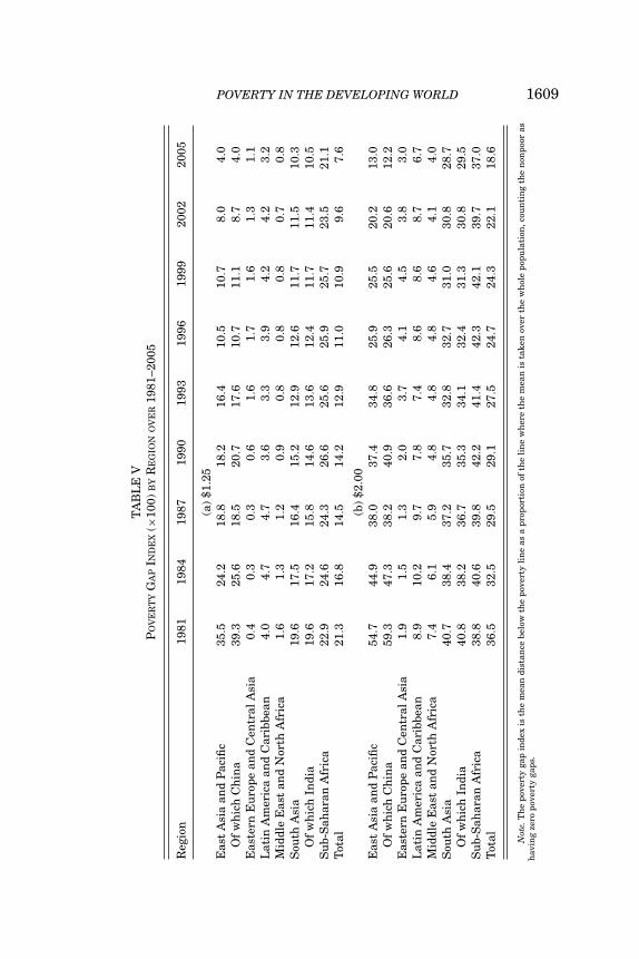
POVERTY IN THE DEVELOPING WORLD 1609
TA
BL
EV
PO
VE
RT
YG
AP
IND
EX
(×10
0)B
YR
EG
ION
OV
ER
1981
–200
5
Reg
ion
1981
1984
1987
1990
1993
1996
1999
2002
2005
(a)
$1.2
5E
ast
Asi
aan
dP
acifi
c35
.524
.218
.818
.216
.410
.510
.78.
04.
0O
fw
hic
hC
hin
a39
.325
.618
.520
.717
.610
.711
.18.
74.
0E
aste
rnE
uro
pean
dC
entr
alA
sia
0.4
0.3
0.3
0.6
1.6
1.7
1.6
1.3
1.1
Lat
inA
mer
ica
and
Car
ibbe
an4.
04.
74.
73.
63.
33.
94.
24.
23.
2M
iddl
eE
ast
and
Nor
thA
fric
a1.
61.
31.
20.
90.
80.
80.
80.
70.
8S
outh
Asi
a19
.617
.516
.415
.212
.912
.611
.711
.510
.3O
fw
hic
hIn
dia
19.6
17.2
15.8
14.6
13.6
12.4
11.7
11.4
10.5
Su
b-S
ahar
anA
fric
a22
.924
.624
.326
.625
.625
.925
.723
.521
.1T
otal
21.3
16.8
14.5
14.2
12.9
11.0
10.9
9.6
7.6
(b)
$2.0
0E
ast
Asi
aan
dP
acifi
c54
.744
.938
.037
.434
.825
.925
.520
.213
.0O
fw
hic
hC
hin
a59
.347
.338
.240
.936
. 626
.325
.620
.612
.2E
aste
rnE
uro
pean
dC
entr
alA
sia
1.9
1.5
1.3
2.0
3.7
4.1
4.5
3.8
3.0
Lat
inA
mer
ica
and
Car
ibbe
an8.
910
.29.
77.
87.
48.
68.
68.
76.
7M
iddl
eE
ast
and
Nor
thA
fric
a7.
46.
15.
94.
84.
84.
84.
64.
14.
0S
outh
Asi
a40
.738
.437
.235
.732
.832
.731
.030
.828
.7O
fw
hic
hIn
dia
40.8
38.2
36.7
35.3
34.1
32.4
31.3
30. 8
29.5
Su
b-S
ahar
anA
fric
a38
.840
.639
.842
.241
.442
.342
.139
.737
.0T
otal
36.5
32.5
29.5
29.1
27.5
24.7
24.3
22.1
18.6
Not
e.T
he
pove
rty
gap
inde
xis
the
mea
ndi
stan
cebe
low
the
pove
rty
lin
eas
apr
opor
tion
ofth
eli
ne
wh
ere
the
mea
nis
take
nov
erth
ew
hol
epo
pula
tion
,cou
nti
ng
the
non
poor
ash
avin
gze
ropo
vert
yga
ps.

1610 QUARTERLY JOURNAL OF ECONOMICS
TA
BL
EV
IM
EA
NC
ON
SU
MP
TIO
NO
FT
HE
PO
OR
($P
ER
DA
Y)
BY
RE
GIO
NO
VE
R19
81–2
005
Reg
ion
1981
1984
1987
1990
1993
1996
1999
2002
2005
(a)
$1.2
5E
ast
Asi
aan
dP
acifi
c0.
680.
790.
810.
830.
850.
880.
870.
890.
95O
fw
hic
hC
hin
a0.
670.
790.
820.
820.
840.
880.
860.
870.
94E
aste
rnE
uro
pean
dC
entr
alA
sia
0.97
0.95
0.95
0.84
0.79
0.78
0.86
0.91
0.89
Lat
inA
mer
ica
and
Car
ibbe
an0.
820.
820.
780.
790.
800.
790.
770.
780.
77M
iddl
eE
ast
and
Nor
thA
fric
a0.
990.
990.
990.
991.
011.
011.
001.
010.
98S
outh
Asi
a0.
840.
860.
870.
880.
910.
910.
920.
920.
93O
fw
hic
hIn
dia
0.84
0.86
0.88
0.89
0.91
0.92
0.92
0.93
0.93
Su
b-S
ahar
anA
fric
a0.
720.
700.
700.
680.
690.
700.
700.
720.
73T
otal
0.74
0.80
0.82
0.82
0.84
0.85
0.85
0.86
0.87
(b)
$2.0
0E
ast
Asi
aan
dP
acifi
c0.
800.
971.
061.
051.
071.
181.
171.
201.
31O
fw
hic
hC
hin
a0.
790.
981.
091.
031.
071.
191.
171.
191.
33E
aste
rnE
uro
pean
dC
entr
alA
sia
1.55
1.56
1.57
1.51
1.38
1.37
1.31
1.29
1.25
Lat
inA
mer
ica
and
Car
ibbe
an1.
221.
221.
201.
231.
211.
211.
211.
241.
26M
iddl
eE
ast
and
Nor
thA
fric
a1.
441.
471.
461.
481.
491.
501.
481.
501.
50S
outh
Asi
a1.
051.
101.
111.
141.
191.
181.
201.
201.
22O
fw
hic
hIn
dia
1.06
1.10
1.12
1.15
1.17
1.19
1.20
1.21
1.22
Su
b-S
ahar
anA
fric
a0.
980.
940.
940.
910.
920.
890.
920.
950.
99T
otal
0.94
1.03
1.08
1.08
1.11
1.14
1.15
1.16
1.21

POVERTY IN THE DEVELOPING WORLD 1611
FIGURE IVPoverty Rates Using Old and New Poverty Lines
of $0.87 (about 3.5% of global GDP per capita). The overall meanconsumption of the poor tended to rise over time, from $0.74 perday in 1981 to $0.87 in 2005 by the $1.25 line, and from $0.94 to$1.21 for the $2 line. Over time, poverty has become shallower inthe world as a whole.
The mean consumption of Africa’s poor not only is lower thanthat for other regions, but also has shown very little increase overtime (Table VI). The same persistence in the depth of poverty isevident in MENA and LAC, though the poor have slightly higheraverage levels of living in both regions. The mean consumption ofEECA’s poor has actually fallen since the 1990s, even though theoverall poverty rate was falling.
VI. COMPARISONS WITH PAST ESTIMATES
Both the $1.25 and $1.45 lines indicate a substantially higherpoverty count in 2005 than obtained using our old $1.08 line in1993 prices; Figure IV compares the poverty rates estimated usingthe latter line with those obtained using either the $1.00- or $1.25-a-day lines at 2005 PPP. Focusing on the $1.25 line, we find that25% of the developing world’s population in 2005 is poor, versus17% using the old line at 1993 PPP—representing an extra 400million people living in poverty. (As can be seen in Figure IV, theseries for $1.00 a day at 2005 PPP tracks closely that for $1.08 at1993 PPP.)
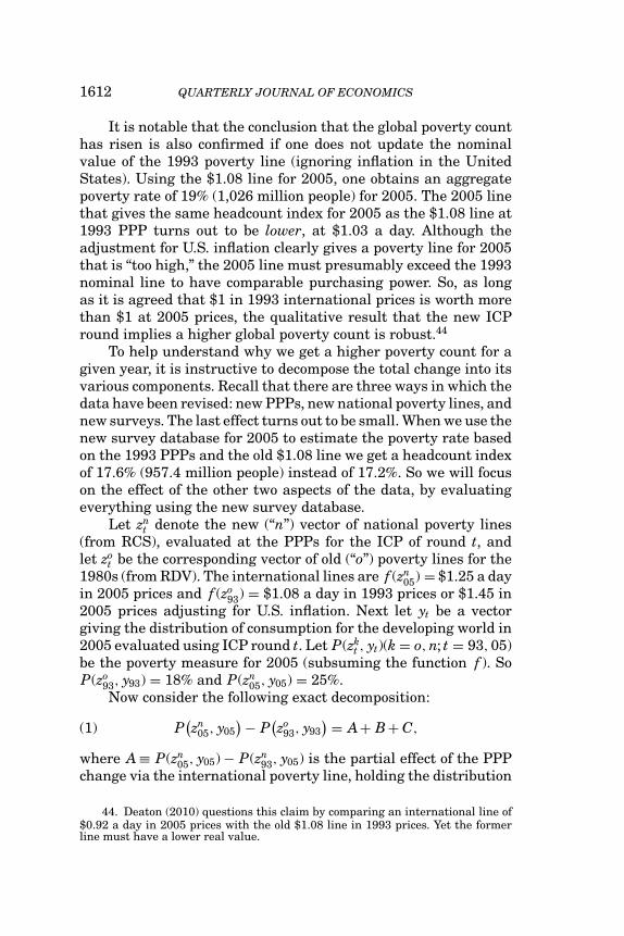
1612 QUARTERLY JOURNAL OF ECONOMICS
It is notable that the conclusion that the global poverty counthas risen is also confirmed if one does not update the nominalvalue of the 1993 poverty line (ignoring inflation in the UnitedStates). Using the $1.08 line for 2005, one obtains an aggregatepoverty rate of 19% (1,026 million people) for 2005. The 2005 linethat gives the same headcount index for 2005 as the $1.08 line at1993 PPP turns out to be lower, at $1.03 a day. Although theadjustment for U.S. inflation clearly gives a poverty line for 2005that is “too high,” the 2005 line must presumably exceed the 1993nominal line to have comparable purchasing power. So, as longas it is agreed that $1 in 1993 international prices is worth morethan $1 at 2005 prices, the qualitative result that the new ICPround implies a higher global poverty count is robust.44
To help understand why we get a higher poverty count for agiven year, it is instructive to decompose the total change into itsvarious components. Recall that there are three ways in which thedata have been revised: new PPPs, new national poverty lines, andnew surveys. The last effect turns out to be small. When we use thenew survey database for 2005 to estimate the poverty rate basedon the 1993 PPPs and the old $1.08 line we get a headcount indexof 17.6% (957.4 million people) instead of 17.2%. So we will focuson the effect of the other two aspects of the data, by evaluatingeverything using the new survey database.
Let znt denote the new (“n”) vector of national poverty lines
(from RCS), evaluated at the PPPs for the ICP of round t, andlet zo
t be the corresponding vector of old (“o”) poverty lines for the1980s (from RDV). The international lines are f (zn
05) = $1.25 a dayin 2005 prices and f (zo
93) = $1.08 a day in 1993 prices or $1.45 in2005 prices adjusting for U.S. inflation. Next let yt be a vectorgiving the distribution of consumption for the developing world in2005 evaluated using ICP round t. Let P(zk
t , yt)(k = o, n; t = 93, 05)be the poverty measure for 2005 (subsuming the function f ). SoP(zo
93, y93) = 18% and P(zn05, y05) = 25%.
Now consider the following exact decomposition:
(1) P(zn
05, y05) − P
(zo
93, y93) = A+ B+ C,
where A ≡ P(zn05, y05) − P(zn
93, y05) is the partial effect of the PPPchange via the international poverty line, holding the distribution
44. Deaton (2010) questions this claim by comparing an international line of$0.92 a day in 2005 prices with the old $1.08 line in 1993 prices. Yet the formerline must have a lower real value.

POVERTY IN THE DEVELOPING WORLD 1613
and national poverty lines constant at their new values; B ≡P(zn
93, y05) − P(zn93, y93) is the partial effect of the change in distri-
bution due to the change in PPPs; and C ≡ P(zn93, y93) − P(zo
93, y93)is the partial effect of updating the data set on national povertylines. Note that A+ B is the total effect (on both the poverty linesand the distribution) of the PPP revisions, holding the data onnational poverty lines constant at their new values.
There are two counterfactual terms in the decomposition in(1), namely P(zn
93, y05) and P(zn93, y93). To evaluate these terms we
need to use the $1.44-a-day line at 1993 PPP (Section III), ratherthan the $1.08 line, which was based on the old RDV compila-tion of poverty lines. In applying this line to the 2005 distributionwe need to update for U.S. inflation, giving zn
93 = $1.95 in 2005prices. We then obtain P(zn
93, y05) = 46% and P(zn93, y93) = 29%.
Comparing these it can be seen that, holding the 1993 interna-tional poverty line constant (in real terms in the United States),the change in the PPPs added 17% to the poverty rate; this re-sults from the higher cost of living in developing countries impliedby the 2005 ICP results. (If instead one makes the comparisonusing the RDV data set on national poverty lines, one obtainsP(zo
93, y05) − P(zo93, y93) = 14%.)
We find that the partial effect of the PPP revisions via theinternational poverty line is to bring the headcount index downsubstantially from 46% to 25% (A = −21%). But there is a largeand almost offsetting upward effect of the change in distribution(B = 17%). On balance the net effect of the change in the PPPs isto bring the poverty rate down from 29% to 25% (A+ B = −4%).The fact that the PPP revisions on their own bring down theoverall poverty count relative to a fixed set of national lines isnot surprising, given that the poverty line is set at the mean oflines for the poorest countries and that the proportionate revisionsto the PPPs tend to be greater for poorer countries. It can beshown that if the international poverty line is that of the poorestcountry, which also has the largest upward revision to its PPP,then the aggregate poverty rate will automatically fall, given thatthe national poverty lines are fixed in local currency units. Theworking paper version provides a proof of this claim (Chen andRavallion 2009). Working against this downward effect of the newPPPs, there is an upward adjustment to the poverty count comingfrom the new data on national poverty lines, which (as we haveseen in Figure II) tend to be higher for the poorest countries thanthose used by RDV for the 1980s. The updating of the data on
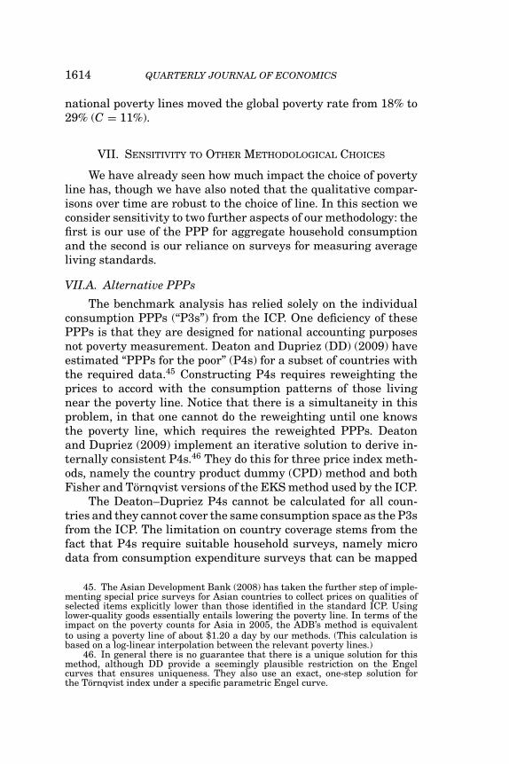
1614 QUARTERLY JOURNAL OF ECONOMICS
national poverty lines moved the global poverty rate from 18% to29% (C = 11%).
VII. SENSITIVITY TO OTHER METHODOLOGICAL CHOICES
We have already seen how much impact the choice of povertyline has, though we have also noted that the qualitative compar-isons over time are robust to the choice of line. In this section weconsider sensitivity to two further aspects of our methodology: thefirst is our use of the PPP for aggregate household consumptionand the second is our reliance on surveys for measuring averageliving standards.
VII.A. Alternative PPPs
The benchmark analysis has relied solely on the individualconsumption PPPs (“P3s”) from the ICP. One deficiency of thesePPPs is that they are designed for national accounting purposesnot poverty measurement. Deaton and Dupriez (DD) (2009) haveestimated “PPPs for the poor” (P4s) for a subset of countries withthe required data.45 Constructing P4s requires reweighting theprices to accord with the consumption patterns of those livingnear the poverty line. Notice that there is a simultaneity in thisproblem, in that one cannot do the reweighting until one knowsthe poverty line, which requires the reweighted PPPs. Deatonand Dupriez (2009) implement an iterative solution to derive in-ternally consistent P4s.46 They do this for three price index meth-ods, namely the country product dummy (CPD) method and bothFisher and Tornqvist versions of the EKS method used by the ICP.
The Deaton–Dupriez P4s cannot be calculated for all coun-tries and they cannot cover the same consumption space as the P3sfrom the ICP. The limitation on country coverage stems from thefact that P4s require suitable household surveys, namely microdata from consumption expenditure surveys that can be mapped
45. The Asian Development Bank (2008) has taken the further step of imple-menting special price surveys for Asian countries to collect prices on qualities ofselected items explicitly lower than those identified in the standard ICP. Usinglower-quality goods essentially entails lowering the poverty line. In terms of theimpact on the poverty counts for Asia in 2005, the ADB’s method is equivalentto using a poverty line of about $1.20 a day by our methods. (This calculation isbased on a log-linear interpolation between the relevant poverty lines.)
46. In general there is no guarantee that there is a unique solution for thismethod, although DD provide a seemingly plausible restriction on the Engelcurves that ensures uniqueness. They also use an exact, one-step solution forthe Tornqvist index under a specific parametric Engel curve.
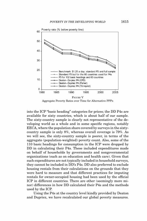
POVERTY IN THE DEVELOPING WORLD 1615
FIGURE VAggregate Poverty Rates over Time for Alternative PPPs
into the ICP “basic heading” categories for prices; the DD P4s areavailable for sixty countries, which is about half of our sample.The sixty-country sample is clearly not representative of the de-veloping world as a whole and in some specific regions, notablyEECA, where the population share covered by surveys in the sixty-country sample is only 8%, whereas overall coverage is 79%. Aswe will see, the sixty-country sample is poorer, in terms of theaggregate (population-weighted) poverty count. Also, some of the110 basic headings for consumption in the ICP were dropped byDD in calculating their P4s. These included expenditures madeon behalf of households by governments and nongovernmentalorganizations (such as on education and health care). Given thatsuch expenditures are not typically included in household surveys,they cannot be included in DD’s P4s. DD also preferred to excludehousing rentals from their calculations on the grounds that theywere hard to measure and that different practices for imputingrentals for owner-occupied housing had been used by the officialICP in different countries. There are other (seemingly more mi-nor) differences in how DD calculated their P4s and the methodsused by the ICP.
Using the P4s at the country level kindly provided by Deatonand Dupriez, we have recalculated our global poverty measures.

1616 QUARTERLY JOURNAL OF ECONOMICS
TA
BL
EV
IIA
GG
RE
GA
TE
PO
VE
RT
YR
AT
EA
ND
RE
GIO
NA
LP
RO
FIL
EF
OR
2005
UN
DE
RA
LTE
RN
AT
IVE
PP
PS
(1)
(2)
(3)
(4)
(5)
(6)
(7)
PP
PP
3P
3P
3P
3P
4:C
PD
P4:
Fis
her
P4:
Tor
nqv
ist
No.
cou
ntr
ies
for
pove
rty
mea
sure
s11
511
560
6060
6060
No.
cou
ntr
ies
for
pove
rty
lin
e15
1514
1414
1414
Pov
erty
lin
e(p
erm
onth
)$3
8.00
$33.
34$3
7.41
$32.
88R
s.57
6.86
Rs.
557.
00R
s.54
7.83
No.
basi
ch
eadi
ngs
110
102
110
102
102
102
102
Hea
dcou
nt
inde
x(%
ofpo
pula
tion
)E
ast
Asi
aan
dP
acifi
c16
.813
.416
.112
.913
.212
.712
.5E
aste
rnE
uro
pean
dC
entr
alA
sia
3.7
3.75
7.1
8.1
4.8
4.1
4.6
Lat
inA
mer
ica
and
Car
ibbe
an8.
27.
18.
47.
68.
88.
57.
9M
iddl
eE
ast
and
Nor
thA
fric
a3.
62.
28.
74.
94.
24.
24.
2S
outh
Asi
a40
.335
.139
.134
.037
.935
.634
.0S
ub-
Sah
aran
Afr
ica
50.9
50.4
49.9
49.6
50.4
50.9
49.8
Tot
al(f
orsa
mpl
edco
un
trie
s)25
.222
.428
.325
.126
.725
.724
.9
Not
e.T
he
Dea
ton
–Du
prie
zP
4ca
lcu
lati
ons
are
only
poss
ible
for
abou
th
alf
the
cou
ntr
ies
inth
efu
llsa
mpl
e,gi
ven
that
con
sum
ptio
nex
pen
ditu
resu
rvey
sar
ere
quir
ed.A
lso,
one
cou
ntr
ydr
ops
out
ofth
ere
fere
nce
grou
pfo
rca
lcu
lati
ng
the
pove
rty
lin
e.T
he
pove
rty
lin
esfo
rco
lum
n(5
)–(7
)P
4sar
eD
eato
n–D
upr
iez
“wor
ldru
pees
.”

POVERTY IN THE DEVELOPING WORLD 1617
In all cases we recalculate the international poverty line under thenew PPPs, as well as (of course) the poverty measures. Table VIIgives the results by region for 2005, whereas Figure V plots the es-timates by year. In both cases we give our benchmark estimates forthe official ICP PPP for individual consumption using all 110 basicheadings for consumption and results for the 102 basic headingscomprising those that can be matched to surveys less the extra fewcategories that DD chose not to include. Because the sixteen coun-tries used by DD did not include one of the fifteen countries in ourreference group, the poverty line is recalculated for fourteen coun-tries, giving a line of $1.23 a day ($37.41 per month). With the helpof the World Bank’s ICP team, we also recalculated the official P3sfor consumption using the set of basic headings chosen by DD. Col-umn (1) reproduces the estimates from Table III, whereas column(2) gives the corresponding estimates for the full sample of coun-tries using P3s calibrated to the 102 basic headings used by DD.Columns (3) and (4) give the results corresponding to columns (1)and (2) using the sixty-country subsample used by DD. Columns(5)–(7) give our estimates of the poverty measures using the P4sfrom DD, for each of their three methods. We give (population-weighted) aggregate results for the sample countries.47
It can be seen from Table VII that the switch from 110 to102 basic headings reduces the aggregate poverty measures byabout three percentage points, whereas switching from the 115-country sample to the 60-country sample has the opposite effect,adding three points. The pure effect of switching from P3 to P4is indicated by comparing column (4) with columns (5)–(7). Thischange has only a small impact using the EKS method (for eitherthe Fischer or Tornqvist indices), though it has a slightly largereffect using the CPD method.
On balance, the aggregate poverty count turns out to be quitesimilar between the P4s and our main estimates using standardP3s on the full sample. If one assumes that the countries with-out household surveys have the regional average poverty rates,then the Fisher P4 gives a count of 1,402 million for the numberof poor, whereas the CPD and Tornqvist P4s give counts of 1,454and 1,359 million, respectively, as compared to 1,377 million using
47. Note that this is a slightly different aggregation method from our earlierresults, which assumed that the sample was representative at regional level. Thatis clearly not plausible for the sixty-country sample used by DD. We have recalcu-lated the aggregates for the 115-country sample under the same basis as for the60-country sample.
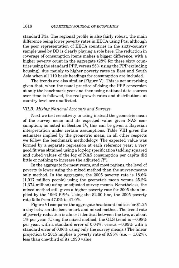
1618 QUARTERLY JOURNAL OF ECONOMICS
standard P3s. The regional profile is also fairly robust, the maindifference being lower poverty rates in EECA using P4s, althoughthe poor representation of EECA countries in the sixty-countrysample used by DD is clearly playing a role here. The reduction incoverage of consumption items makes a bigger difference, with ahigher poverty count in the aggregate (28% for these sixty coun-tries using the standard PPP, versus 25% using the PPP excludinghousing), due mainly to higher poverty rates in East and SouthAsia when all 110 basic headings for consumption are included.
The trends are also similar (Figure V). This is not surprisinggiven that, when the usual practice of doing the PPP conversionat only the benchmark year and then using national data sourcesover time is followed, the real growth rates and distributions atcountry level are unaffected.
VII.B. Mixing National Accounts and Surveys
Next we test sensitivity to using instead the geometric meanof the survey mean and its expected value given NAS con-sumption; as noted in Section IV, this can be given a Bayesianinterpretation under certain assumptions. Table VIII gives theestimates implied by the geometric mean; in all other respectswe follow the benchmark methodology. The expected value wasformed by a separate regression at each reference year; a verygood fit was obtained using a log-log specification (adding squaredand cubed values of the log of NAS consumption per capita didlittle or nothing to increase the adjusted R2).
In the aggregate for most years, and most regions, the level ofpoverty is lower using the mixed method than the survey-meansonly method. In the aggregate, the 2005 poverty rate is 18.6%(1,017 million people) using the geometric mean versus 25.2%(1,374 million) using unadjusted survey means. Nonetheless, themixed method still gives a higher poverty rate for 2005 than im-plied by the 1993 PPPs. Using the $2.00 line, the 2005 povertyrate falls from 47.0% to 41.0%.
Figure VI compares the aggregate headcount indices for $1.25a day between the benchmark and mixed method. The trend rateof poverty reduction is almost identical between the two, at about1% per year. (Using the mixed method, the OLS trend is −0.98%per year, with a standard error of 0.04%, versus −0.99% with astandard error of 0.06% using only the survey means.) The linearprojection to 2015 implies a poverty rate of 9.95% (s.e. = 1.02%),less than one-third of its 1990 value.

POVERTY IN THE DEVELOPING WORLD 1619
TABLE VIIIHEADCOUNT INDEX USING MIXED METHOD (%)
1981 1984 1987 1990 1993 1996 1999 2002 2005
(a) $1.25 a dayEast Asia and Pacific 67.1 57.4 49.4 48.5 40.6 28.4 26.5 20.3 12.1
Of which China 73.0 62.3 51.9 55.5 45.0 30.6 29.0 22.4 12.1Europe and Central Asia 1.9 1.7 1.7 2.6 4.8 6.1 5.7 3.8 3.1Latin America 13.9 16.3 16.7 18.0 15.0 15.8 14.0 15.3 9.8
and CaribbeanMiddle East 7.6 6.5 6.4 5.0 5.0 5.4 5.4 4.4 4.4
and North AfricaSouth Asia 42.7 39.3 39.0 33.6 30.4 28.1 28.1 26.2 21.6
Of which India 42.3 38.7 38.0 32.2 30.4 26.4 26.4 25.1 20.3Sub-Saharan Africa 51.9 54.0 53.7 55.6 55.9 56.5 56.9 55.3 51.0Total 43.6 39.6 36.6 35.3 31.7 27.2 26.5 23.7 18.6
(b) $2.00 a dayEast Asia and Pacific 89.8 86.0 81.4 78.6 73.0 59.6 56.2 46.6 34.0
Of which China 95.4 91.6 85.7 85.4 78.4 63.0 58.8 48.8 33.9Europe and Central Asia 6.9 6.4 5.8 7.4 11.8 14.7 14.8 10.8 8.2Latin America 26.5 30.3 29.2 31.8 28.2 29.3 26.4 28.7 19.6
and CaribbeanMiddle East 26.7 24.4 24.0 20.7 20.5 20.7 19.8 17.5 15.8
and North AfricaSouth Asia 77.4 75.0 74.7 70.1 67.9 65.4 64.5 62.6 56.8
Of which India 77.0 74.6 74.2 69.3 68.4 64.2 63.9 62.4 57.0Sub-Saharan Africa 73.1 74.8 74.2 75.2 75.2 76.6 76.9 76.0 73.4Total 66.0 64.4 62.5 60.7 58.4 53.7 52.2 48.2 41.0
The mixed method gives a higher poverty rate for LAC andMENA and makes negligible difference for SSA. Other regionssee a lower poverty rate. The $1.25-a-day rate for East Asia in2005 falls from 17% to 12%. The largest change is for South Asia,where by 2005 the poverty rate for India falls to about 20% usingthe mixed method versus 42% using the unadjusted survey means;the proportionate gap was considerable lower in 1981 (42% usingthe mixed method versus 60% using the survey mean alone).
India accounts for a large share of the discrepancies be-tween the levels of poverty between the benchmark and the mixedmethod, reflecting both the country’s population weight and thelarge gap that has emerged in recent times between the survey-based and national accounts consumption aggregates for India.Figure VI also gives the complete series for $1.25 a day excludingIndia; it can be seen that the gap between the two methods nar-rows over time. If we focus on the poverty rates for the developing
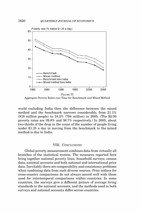
1620 QUARTERLY JOURNAL OF ECONOMICS
FIGURE VIAggregate Poverty Rates over Time for Benchmark and Mixed Method
world excluding India then the difference between the mixedmethod and the benchmark narrows considerably, from 21.1%(918 million people) to 18.2% (794 million) in 2005. (The $2.00poverty rates are 39.8% and 36.7% respectively.) In 2005, abouttwo-thirds of the drop in the count of the number of people livingunder $1.25 a day in moving from the benchmark to the mixedmethod is due to India.
VIII. CONCLUSIONS
Global poverty measurement combines data from virtually allbranches of the statistical system. The measures reported herebring together national poverty lines, household surveys, censusdata, national accounts and both national and international pricedata. Inevitably there are comparability and consistency problemswhen combining data from such diverse sources. Price indices forcross-country comparisons do not always accord well with thoseused for intertemporal comparisons within countries. In somecountries, the surveys give a different picture of average livingstandards to the national accounts, and the methods used in bothsurveys and national accounts differ across countries.

POVERTY IN THE DEVELOPING WORLD 1621
However, thanks to the efforts and support of governmen-tal statistics offices and international agencies, and improvedtechnologies, the available data on the three key ingredients ininternational poverty measurement—national poverty lines, rep-resentative samples of household consumption expenditures (orincomes) and data on prices—have improved greatly since globalpoverty monitoring began. The expansion of country-level povertyassessments since the early 1990s has greatly increased the dataavailable on national poverty lines. Side-by-side with this, thecountry coverage of credible household survey data, suitable formeasuring poverty, has improved markedly, the frequency of datahas increased, public access to these data has improved, and thelags in data availability have been reduced appreciably. And withthe substantial global effort that went into the 2005 InternationalComparison Program we are also in a better position to assurethat the poverty lines used in different countries have similarpurchasing power, so that two people living in different countriesbut with the same real standard of living are treated the sameway. The results of the 2005 ICP imply a higher cost of livingin developing countries than past ICP data have indicated; the“Penn effect” is still evident, but it has been overstated.
We have combined the new data on prices from the 2005 ICPand household surveys with a new compilation of national povertylines, which updates (by fifteen years on average) the old nationallines used to set the original $1-a-day line. Importantly, the newcompilation of national lines is more representative of developingcountries, given that the sample size is larger and it corrects thesample biases in the old data set. The pure effect of the PPPrevisions is to bring the poverty count down but this is outweighedby the higher level of the national poverty lines in the poorestcountries, as used to determine the international line.
Our new calculations using the 2005 ICP and new interna-tional poverty line of $1.25 a day imply that 25% of the populationof the developing world, 1.4 billion people, were poor in 2005,which is 400 million more for that year 2005 than implied by ourold international poverty line based on national lines for the 1980sand the 1993 ICP. In China alone, which had not previously par-ticipated officially in the ICP, the new PPP implies that an extra10% of the population is living below our international povertyline. But the impact is not confined to China; there are upwardrevisions to our past estimates for all regions. The higher globalcount is in no small measure the result of correcting the sample
1622 QUARTERLY JOURNAL OF ECONOMICS
bias in the original compilation of national poverty lines used toset the old “$1-a-day” line.
Although there are a number of data and methodologicalissues that caution against comparisons across different sets ofPPPs, it is notable that our poverty count for 2005 is quite robustto using alternative PPPs anchored to the consumption patternsof those living near the poverty line. Of course, different meth-ods of determining the international poverty line give differentpoverty counts. If we use a line of $1.00 a day at 2005 PPP (almostexactly India’s official poverty line) then we get a poverty rate of16%—slightly under 900 million people—whereas if we use themedian poverty line for all developing countries in our poverty-line sample, namely $2.00 a day, then the poverty rate rises to50%, slightly more than two billion people.
As a further sensitivity test we have proposed a simpleBayesian method of mixing the data on consumption from thenational accounts consumption with that from survey means,whereby the survey mean is replaced by the geometric mean ofthe survey mean and its predicted value based on prior nationalaccounts data. This is justified only under potentially strong as-sumptions, notably that consumption is identically log-normallydistributed between the (national-accounts-based) prior and thesurveys. These assumptions can be questioned, but they do atleast provide a clear basis for an alternative hybrid estimator.This gives a lower poverty count for 2005, namely 19% living be-low $1.25 a day rather than 25%. A large share of this gap—two-thirds of the drop in the count of the number of poor in switching tothe mixed method—is due to India’s (unusually large) discrepancybetween consumption measured in the national accounts and thatmeasured by surveys.
Although the new data suggest that the developing world ispoorer than we thought, it has been no less successful in reducingthe incidence of absolute poverty since the early 1980s. Indeed,the overall rate of progress against poverty is fairly similar topast estimates and robust to our various changes in methodology.The trend rate of global poverty reduction of 1% per year turnsout to be slightly higher than we had estimated previously, duemainly to the higher weight on China’s remarkable pace of povertyreduction. The trend is even higher if we use our Bayesian mixed-method. The developing world as a whole is clearly still on trackto attaining the first Millennium Development Goal of halvingthe 1990s “extreme poverty” rate by 2015. China attained the

POVERTY IN THE DEVELOPING WORLD 1623
MDG early in the millennium, almost 15 years ahead of the targetdate.
However, the developing world outside China will not attainthe MDG without a higher rate of poverty reduction than we haveseen over 1981–2005. The persistently high incidence and depthof poverty in SSA are particularly notable. There are encouragingsigns of progress in this region since the late 1990s, although lagsin survey data availability and problems of comparability andcoverage leave us unsure about how robust this will prove to be.
DEVELOPMENT RESEARCH GROUP, WORLD BANK
DEVELOPMENT RESEARCH GROUP, WORLD BANK
REFERENCES
Ackland, Robert, Steve Dowrick, and Benoit Freyens, “Measuring Global Poverty:Why PPP Methods Matter,” Australian National University, Canberra, Mimeo,2007.
African Development Bank, Comparative Consumption and Price Levels in AfricanCountries (Tunis, Tunisia: African Development Bank, 2007).
Ahmad, Sultan, “Purchasing Power Parity for International Comparison ofPoverty: Sources and Methods,” Development Data Group, World Bank, 2003.
Asian Development Bank, Comparing Poverty Across Countries: The Role of Pur-chasing Power Parities (Manila, the Philippines: Asian Development Bank,2008).
Atkinson, Anthony B., “On the Measurement of Poverty,” Econometrica, 55 (1987),749–764.
Balassa, Bela, “The Purchasing Power Parity Doctrine: A Reappraisal,” Journal ofPolitical Economy, 72 (1964), 584–596.
Bhalla, Surjit, Imagine There’s No Country: Poverty, Inequality and Growth in theEra of Globalization (Washington, DC: Institute for International Economics,2002).
Bidani, Benu, and Martin Ravallion, “A New Regional Poverty Profile for Indone-sia,” Bulletin of Indonesian Economic Studies, 29 (1993), 37–68.
Bourguignon, Francois, and Christian Morrisson, “Inequality among World Citi-zens: 1820–1992,” American Economic Review, 92 (2002), 727–744.
Central Statistical Organization, Report of the Group for Examining Discrepancyin PFCE Estimates from NSSO Consumer Expenditure Data and EstimatesCompiled by National Accounts Division (New Delhi: Central Statistical Or-ganization, Ministry of Statistics, Government of India, 2008).
Chaudhuri, Shubham, and Martin Ravallion, “How Well Do Static Indicators Iden-tify the Chronically Poor?” Journal of Public Economics, 53 (1994), 367–394.
Chaudhury, Nazmul, Jeffrey Hammer, Michael Kremer, Karthik Muralidharan,and F. Halsey Rogers, “Missing in Action: Teacher and Health Worker Absencein Developing Countries,” Journal of Economic Perspectives, 20 (2006), 91–116.
Chen, Shaohua, and Martin Ravallion, “How Did the World’s Poor Fare in the1990s?” Review of Income and Wealth, 47 (2001), 283–300.
——, “How Have the World’s Poorest Fared since the Early 1980s?” World BankResearch Observer, 19 (2004), 141–70.
——, “Absolute Poverty Measures for the Developing World, 1981–2004,” Proceed-ings of the National Academy of Sciences, 104 (2007), 16,757–16,762.
——, “The Developing World Is Poorer Than We Thought, But No Less Successfulin the Fight against Poverty,” World Bank Policy Research Working Paper4703, 2009.

1624 QUARTERLY JOURNAL OF ECONOMICS
——, “China Is Poorer Than We Thought, But No Less Successful in the Fightagainst Poverty,” in Debates on the Measurement of Poverty, Sudhir Anand,Paul Segal, and Joseph Stiglitz, eds. (Oxford, UK: Oxford University Press,2010).
Cuthbert, James R., and Margaret Cuthbert, “On Aggregation Methods of Pur-chasing Power Parities,” Working Paper 56, Department of Economics andStatistics, OECD, Paris, 1988.
Dalgaard, Esben, and Henrik Sørensen, “Consistency between PPP Benchmarksand National Price and Volume Indices,” Paper Presented at the 27th Gen-eral Conference of the International Association for Research on Income andWealth, Sweden, 2002.
Deaton, Angus, “Measuring Poverty in a Growing World (or Measuring Growth ina Poor World),” Review of Economics and Statistics, 87 (2005), 353–378.
——, “Price Indexes, Inequality, and the Measurement of World Poverty,” Presi-dential Address to the American Economics Association, Atlanta, GA, 2010.
Deaton, Angus, and Olivier Dupriez, “Global Poverty and Global Price Indices,”Development Data Group, World Bank, Mimeo, 2009.
Deaton, Angus, and Alan Heston, “Understanding PPPs and PPP-Based NationalAccounts,” American Economic Journal: Macroeconomics, forthcoming, 2010.
Deaton, Angus, and Salman Zaidi, “Guidelines for Constructing Consumption Ag-gregates for Welfare Analysis,” World Bank Living Standards MeasurementStudy Working Paper 135, 2002.
Diewert, Erwin, “New Methodology for Linking Regional PPPs,” InternationalComparison Program Bulletin, 5 (2008), 10–14.
Groves, Robert E., and Mick P. Couper, Nonresponse in Household Interview Sur-veys (New York: Wiley, 1998).
Hansen, Bruce E., “Sample Splitting and Threshold Estimation,” Econometrica,68 (2000), 575–603.
Ikle, Doris, “A New Approach to the Index Number Problem,” Quarterly Journalof Economics, 86 (1972), 188–211.
Karshenas, Massoud, “Global Poverty: National Accounts Based versus SurveyBased Estimates,” Development and Change, 34 (2003), 683–712.
Korinek, Anton, Johan Mistiaen, and Martin Ravallion, “Survey Nonresponse andthe Distribution of Income,” Journal of Economic Inequality, 4 (2006), 33–55.
——, “An Econometric Method of Correcting for Unit Nonresponse Bias in Sur-veys,” Journal of Econometrics, 136 (2007), 213–235.
Lanjouw, Peter, and Martin Ravallion, “Poverty and Household Size,” EconomicJournal, 105 (1995), 1415–1435.
Lopez, Humberto, and Luis Serven, “A Normal Relationship? Poverty, Growth andInequality,” World Bank Policy Research Working Paper 3814, 2006.
Nuxoll, Daniel A., “Differences in Relative Prices and International Differences inGrowth Rates,” American Economic Review, 84 (1994), 1423–1436.
Pinkovskiy, Maxim, and Xavier Sala-i-Martin, “Parametric Estimations of theWorld Distribution of Income,” NBER Working Paper 15433, 2009.
Planning Commission, Report of the Expert Group to Review the Methodologyfor Estimation of Poverty (New Delhi: Planning Commission, Government ofIndia, 2009).
Ravallion, Martin, Poverty Comparisons (Chur, Switzerland: Harwood AcademicPress, 1994).
——, “Measuring Aggregate Economic Welfare in Developing Countries: How WellDo National Accounts and Surveys Agree?” Review of Economics and Statis-tics, 85 (2003), 645–652.
——, “A Global Perspective on Poverty in India,” Economic and Political Weekly,43 (2008a), 31–37.
——, “On the Welfarist Rationale for Relative Poverty Lines,” in Social Welfare,Moral Philosophy and Development: Essays in Honour of Amartya Sen’s Sev-enty Fifth Birthday, Kaushik Basu and Ravi Kanbur, eds. (Oxford: OxfordUniversity Press, 2008b).
——, “Poverty Lines,” in The New Palgrave Dictionary of Economics, Larry Blumeand Steven Durlauf, eds. (London: Palgrave Macmillan, 2008c).
——, “Understanding PPPs and PPP-Based National Accounts: A Comment,”American Economic Journal: Macroeconomics, forthcoming, 2010.

POVERTY IN THE DEVELOPING WORLD 1625
Ravallion, Martin, and Shaohua Chen, “China’s (Uneven) Progress againstPoverty,” Journal of Development Economics, 82 (2007), 1–42.
——, “Weakly Relative Poverty,” Review of Economics and Statistics, in press,2010.
Ravallion, Martin, Shaohua Chen, and Prem Sangraula, “New Evidence on the Ur-banization of Global Poverty,” Population and Development Review, 33 (2007),667–702.
——, “Dollar a Day Revisited,” World Bank Economic Review, 23 (2009), 163–184.Ravallion, Martin, Gaurav Datt, and Dominique van de Walle, “Quantifying Ab-
solute Poverty in the Developing World,” Review of Income and Wealth, 37(1991), 345–361.
Sala-i-Martin, Xavier, “The World Distribution of Income: Falling Poverty and . . .Convergence. Period,” Quarterly Journal of Economics, 121 (2006), 351–397.
Samuelson, Paul, “Theoretical Notes on Trade Problems,” Review of Economicsand Statistics, 46 (1964), 145–154.
Slesnick, Daniel, “Empirical Approaches to Measuring Welfare,” Journal of Eco-nomic Literature, 36 (1998), 2108–2165.
Summers, Robert, and Alan Heston, “The Penn World Table (Mark 5): An Ex-tended Set of International Comparisons, 1950–1988,” Quarterly Journal ofEconomics, 106 (1991), 327–368.
United Nations, Evaluation of the International Comparison Programme (NewYork: UN Statistics Division, 1998).
World Bank, World Development Report: Poverty (New York: Oxford UniversityPress, 1990).
——, India: Achievements and Challenges in Reducing Poverty, Report No. 16483-IN, 1997.
——, Comparisons of New 2005 PPPs with Previous Estimates (Revised AppendixG to World Bank [2008b]) (www.worldbank.org/data/icp, 2008a).
——, Global Purchasing Power Parities and Real Expenditures. 2005 InternationalComparison Program (www.worldbank.org/data/icp, 2008b).