aftermath issue 5 1 - university of western...

AfterMath Issue 5 1

Contributors

Editors: Wilson Ong, Minh Van Nguyen (typesetter for this issue)

Writers for this issue: Mark Ioppolo, Alasdair McAndrew, Minh Van Nguyen, WilsonOng

If you wish to contribute to the next issue of AfterMath, please email Wilson Ong(ongw03[at]student.uwa.edu.au).

Website: http://www.maths.uwa.edu.au/~MSMailing list: [email protected]

AfterMath Issue 5 2

Contents

The Hairy Ball Theorem 3Mark Ioppolo

Differential Inequalities 6Wilson Ong

A Morsel of Maxima 8Alasdair McAndrew

Number Theory and Cryptography using PARI/GP 21Minh Van Nguyen

Jokes Corner 30

Problems Section 31

AfterMath Issue 5 3

The Hairy Ball TheoremMark Ioppolo

1 Introduction

The surface of the earth is almost spherical. At any point close to the Earth’s surface,we can measure the velocity of the wind at that point. In other words, we can definea vector field corresponding to a velocity field at any point close to the Earth. I nowclaim that at any point in time, there is at least one point on the Earth where there isno wind. Moreover, surrounding this point will be a cyclone (not necessarily a large one,perhaps just a twist in the wind). This strange claim can be verified via one of the mostcommonly stated theorems of topology, the Hairy Ball Theorem (HBT). I came acrossthis result whilst working on an assignment with fellow undergraduate Chris Mofflin. Ourtask was to explain in depth and prove the HBT, along with the closely related Brouwerfixed point theorem. In this article, I will discuss only the former.

2 What is the Hairy Ball Theorem?

The Hairy Ball Theorem was first conjectured by Frenchman Henri Poincare in the late19th century. The version conjectured by Poincare states that there is no continuousnon-zero tangential vector field on a two dimensional sphere. We can see where the namecomes from by thinking of each vector as a “hair” growing out of some point on thesphere. For this reason, the theorem is commonly stated as “you can’t comb the hairson a hairy ball flat without creating a cowlick” or “you can’t comb the hair on a billiardball,” as the act of combing the ball is equivalent to defining a vector field on its surface.While Poincare [3] was able to prove his version of the theorem, it was not until 1912 thatthe general case was proved by the Dutch mathematician L.E.J Brouwer [1]. Brouwerwas able to demonstrate that Poincare’s theorem was not only true for a two dimensionalsphere, but indeed it holds true for any even dimensional sphere.

3 So how about a proof?

The HBT is not very difficult to prove via orthodox methods. However, one needs to havealgebraic or differential topology or advanced calculus on their tool belt to understand it.For this reason, I would like to present a very clever proof suggested by John Milnor [2]that uses ideas that are more accessible to a non-mathematician. Milnor relies on twosimple lemmas to prove a special case of the theorem, from which the general case is aresult.

3.1 Milnor’s lemmas

Lemma 1. Let A be a compact region in Rn and let V (x) be a continuously differentiable

vector field which is defined throughout a neighbourhood of A. For each t ∈ R, defineft(x) = x + tV (x). If the parameter t is sufficiently small, then the mapping ft is one-to-one and transforms the region A onto a nearby region ft(A) whose volume can beexpressed as a polynomial function of t.

AfterMath Issue 5 4

Lemma 2. If the parameter t is sufficiently small, then the transformation x 7→ x+tV (x)(where |V (x)| = 1) maps the unit sphere in R

n onto the sphere of radius r =√

1 + t2.

The proofs of Lemmas 1 and 2 have been omitted. However, I encourage the reader torefer to [2]. Not only are they fundamental in understanding the material, but they arealso very interesting.

3.2 A proof of the Hairy Ball Theorem

Theorem 1. (HBT: weak version) An even-dimensional sphere does not possess anycontinuously differentiable field of non-zero unit tangent vectors.

Proof. Let A be a region between two concentric spheres defined by

A = {x ∈ Rn | a ≤ ‖x‖ ≤ b}

We extend the vector field V through this region by setting

V (rx) = rV (x)

for r ∈ [a, b]. It follows that the mapping ft(x) = x + tV (x) is defined throughout A andmaps the sphere of radius r onto the sphere of radius r

√1 + t2, provided t is sufficiently

small. Hence, it maps A onto the region between two spheres of radius a√

1 + t2 andb√

1 + t2. Then we can state the volume of the transformed region as

Vol(ft(A)) = (√

1 + t2)nVol(A) (1)

We next prove equation (1).

Clearly, (1) follows from a change of variable of integration. As mentioned above, ft(x)maps A = {x ∈ R

n | a ≤ ‖x‖ ≤ b} onto A′ = {x ∈ Rn | a

√1 + t2 ≤ ‖x‖ ≤

b√

1 + t2}. Hence ft(A) = A′. Define the bijection ψ : A −→ A′ via ψ(x) =√

1 + t2x =√1 + t2In×nx. Also, observe that A′ =

√1 + t2A. Thus

Vol(A′) =

∫

· · ·∫

A′

1 dV =

∫

· · ·∫

A

1 |det(Jψ)| dV

=

∫

· · ·∫

A

1(√

1 + t2)n dV = (√

1 + t2)n∫

· · ·∫

A

1 dV

= (√

1 + t2)nVol(A)

where the second equality follows from the change of variables formula for multiple inte-grals with Jψ =

√1 + t2In×n, and the integral is n dimensional. Hence

Vol(ft(A)) = Vol(A′) = (√

1 + t2)nVol(A)

For n odd, this volume is not a polynomial function of t, which contradicts Lemma 1.

Theorem 2. (HBT: strong version) An even-dimensional sphere does not possessany continuous field of non-zero tangent vectors.

AfterMath Issue 5 5

Proof. Suppose we can define a continuous non-zero vector field V (u) on Sn−1. Since allof the vectors defined on Sn−1 are non-zero, there must be a vector of minimum length. Solet m > 0 be the minimum of ‖V (u)‖. Then by the Weierstrass Approximation Theorem,there exists a polynomial mapping p : Sn−1 −→ R

n such that

‖p(u)− V (u)‖ <m

2(2)

for all vectors u. We define another vector field W (u) by the formula

W (u) = p(u)− (p(u) · u)u

for all u. The computation W (u) ·u = 0 shows that W (u) is tangent to Sn−1 at u, whilethe computation

‖W (u)− p(u)‖ = |p(u) · u| < m

2(3)

together with the triangle inequality show that W (u) 6= 0.

Adding (2) and (3) yields

‖W (u)− V (u)‖ ≤ ‖p(u)− V (u)‖+ ‖W (u)− p(u)‖ < m ≤ ‖V (u)‖

where the last inequality follows by definition of m. Now assuming W (u) = 0 yields a

contradiction. Then by definition, the quotient W (u)‖W (u)‖ is an infinitely differential field of

unit tangent vectors on Sn−1. If n is even, this is impossible by Theorem 1.

Notice that the strong form does not require the vector field to be differentiable or consistof unit vectors. At this point, Milnor goes on to prove Brouwer’s fixed point theoremwith relative ease. However, this result is saved for another day.

I will finish off by pointing out that the Hairy Ball Theorem can be applied to anyobject homeomorphic to an even-dimensional sphere, i.e. objects that can be continu-ously deformed into an even-dimensional sphere. More information can be found in mostintroductory topology textbooks.

References

[1] L. E. J. Brouwer. Uber Abbildung von Mannigfaltigkeiten. Math. Ann., pages 97–115, 1912.[2] J. Milnor. Analytic proofs of the “Hairy Ball Theorem” and the Brouwer Fixed Point

Theorem. The American Mathematical Monthly, 85(7):521–524, 1978.[3] H. Poincare. Sur les courbes definies par les equations differentielles. J. Math. Pures. Appl.,

4(1):167–244, 1885.

AfterMath Issue 5 6

Differential InequalitiesWilson Ong

Consider the ordinary differential equation

F (x, y, y, . . . , y(n)) = 0 (1)

Suppose that the y(i)’s are subject to certain conditions so that (1) has unique solutiony(t) = f(t). This article examines some simple cases where we can replace the equalitysign in both (1) and it’s solution with an inequality sign.

1 Gronwall’s inequality

Let y(t) and c(t) be functions defined on [a, b), with c(t) continuous. Then the ho-mogeneous first order linear ODE y(t) = c(t)y(t) with y(a) = A, has unique solution

y(t) = AeR

t

ac(u) du.

Gronwall’s inequality asserts that if

y(t) ≤ c(t)y(t) (2)

with y(a) = A, then

y(t) ≤ AeR

t

ac(u) du (3)

The proof of Gronwall’s inequality is analogous to solving the corresponding differentialequation using integrating factors.

By (2), we have

d

dty(t)e−

R

t

ac(u) du = y(t)e−

R

t

ac(u) du − c(t)y(t)e−

R

t

ac(u) du ≤ 0

Here we use the continuity of c(t) to ensure ddt

∫ t

ac(u) du = c(t) by the Fundamental

Theorem of Calculus. Integrating over [a, v],

∫ v

a

d

dty(t)e−

R

t

ac(u) du dt = y(v)e−

R

v

ac(u) du − y(a) ≤ 0

for v ∈ [a, b), and the result follows. It is clear from the proof that the ≤ in (2) and (3)may be replaced by ≥, < or >.

2 A second order differential inequality

Consider the homogeneous second order linear ODE y(t) + y(t) = 0. This has generalsolution y(t) = c1 cos t + c2 sin t. Imposing the initial conditions y(0) = 0 and y(0) = A

yields the unique solution y(t) = A sin t.

Let y(t) be a function on [0, π2). We can show that if

y(t) + y(t) ≥ 0 (4)

AfterMath Issue 5 7

with y(0) = 0 and y(0) = A, then

y(t) ≥ A sin t (5)

Let x(t) = y(t)sin t

= y(t) csc t for t ∈ (0, π2). Now

x(t) = y(t) csc t+ y(t)(− csc t cot t) = (y(t)− y(t) cot t) csc t

and

x = (y(t)− y(t) cot t) (− csc t cot t) +(y(t)− y(t) cot t− y(t)(− csc2 t)

)csc t

= y(t) csc t− 2y(t) csc t cot t+ y(t) csc t(csc2 t+ cot2 t

)

≥− 2y(t) csc t cot t+ y(t) csc t(csc2 t− 1 + cot2 t

)[as y(t) csc t ≥ −y(t) csc t by (4)]

= −2 (y(t)− y(t) cot t) csc t cot t[since csc2 t− 1 ≡ cot2 t

]

= −2x(t) cot t

So x(t) satisfies x(t) ≥ −2x(t) cot t⇐⇒ −x(t) sin t ≤ 2x(t) cos t for t ∈ (0, π2).

Now consider z(t) = x(t) sin2 t = y(t) sin t− y(t) cos t. We have

z(t) = x(t) sin2 t+ 2x(t) sin t cos t ≥ x(t) sin2 t− x(t) sin2 t = 0

wherelimt→0+

z(t) = 0 =⇒ z(t) ≥ 0

Thus x(t) ≥ 0. Now y(0) = 0, so by L’Hopital’s rule, limt→0+ x(t) = y(0)cos 0

= A. Hencex(t) ≥ A =⇒ y(t) ≥ A sin t for t ∈ [0, π

2).

Again this proof shows that the ≥ sign in (4) and (5) may be replaced by ≤, < or >.

The converse is false if A > 0, as shown by the following counterexample. Considery(t) = A

(sin t− t2(t− π

2))≥ A sin t on [0, π

2). Then we have

y(0) = 0

y(t) = A(cos t− 3t2 + πt

)=⇒ y(0) = A

y(t) = A (− sin t− 6t+ π)

y(t) + y(t) = A(

−t3 +π

2t2 − 6t+ π

)

= A

(

−7 +3π

2

)

< A

(

−7 +3(4)

2

)

< 0

when t = 1. So here (5) holds with y(0) = 0 and y(0) = A, but (4) does not hold. Thecase for A ≤ 0 is left as an exercise for the reader.

AfterMath Issue 5 8

A Morsel of MaximaAlasdair McAndrew

[email protected]

This article is an abridged version of the information presented to the RGMIA group [7]at a seminar titled “Maxima: An Open-Source Computer Algebra System”, given on26 March 2007. We’ll first provide a brief history of Maxima (section 1) and then sketchthe state of this software as of March 2007 (section 2). Section 3 contains a discussion ofinterfaces for working with Maxima, whereas section 4 surveys some of the features thatare useful for beginners. The remaining sections briefly evaluate Maxima and concludethis article.

1 A bit of history

Maxima [5] is a descendant of the computer algebra system (CAS) Macsyma, which wasinitially developed at Massachusetts Institute of Technology as part of Project MAC inthe late 1960s. By the mid 1980s, although early versions of Mathematica and Maple werethen gaining market share, Macsyma was clearly the strongest such system, with robustsymbolics, excellent interfaces, and a fine hypertext help system. Macsyma was writtenin the Maclisp dialect of lisp, a language which many considered perfect for mathematicalcomputations.

In 1982, William Schelter, of the University of Texas at Austin, had managed to acquirethe source code to a version of Macsyma which had been licensed to the US Department ofEnergy; this version was known as DOE Macsyma. The source code, adapted by Schelterfor common lisp, was released under the GNU General Public License (GPL) by Schelterin 1998. Schelter maintained this version of Macsyma (renamed GNU Maxima) until hisdeath from a heart attack in 2001, at the untimely age of 52. Since then, Maxima hasbeen maintained by an enthusiastic group of developers, including several of the originaldevelopers of Macsyma.

The original Macsyma, although sold as a commercial package until the mid 1990s, lostground to Maple and Mathematica partly because of some poor business decisions, andpartly because of some of its weaknesses—in particular its numerics. However, such wasthe power and strength of Macsyma that some commentators believe that Maple andMathematica have taken decades to get to the stage where Macsyma was.

As of 2007, Macsyma still exists, and has been acquired by a holding company Tene-dos LLC; this company had previously bought Symbolics, the distributor of Macsyma.Tenedos LLC has not released Macsyma again, or resold it. Symbolics still officially sellMacsyma.

2 Maxima now

To all intents and purposes, Macsyma is now unobtainable and the best current versionof this once-great CAS is Maxima. Maxima has several points in its favour:

AfterMath Issue 5 9

• it is licensed under the GPL; it is now, and always will be, free.

• it is being actively developed.

• the Maxima mailing list [4] is extremely active.

• because Maxima is being developed by its users, it is very attuned to its usercommunity.

• Maxima, in its current form, has excellent calculus, linear algebra, and generalsymbolic capabilities.

However, being based on an early version of Macsyma, many of the later refinements ofMacsyma—believed to be in the order of 50 man-years of work—have not made it as faras Maxima (yet). So Maxima is deficient in some areas:

• its interface is non-standard, a bit clunky and described as “something out of the1970s”.

• it is very weak in discrete mathematics.

• its numerics are still weak—there is still no robust solid method for finding numericroots of (systems of) nonlinear equations.

• its plotting is based on Gnuplot, which is good at plotting functions y = f(x) orz = f(x, y) and for plotting data sets, but not for much else. It can’t, for example,plot two surfaces at once and so show their intersections.

• Maxima does not have a Package system, such as Maple and MuPAD; individualfiles can be loaded into a running session, and a single file may contain one or moreMaxima commands.

• in its current form, Maxima is unsuitable as a teaching tool.

Maxima’s home on the Web is at

http://maxima.sourceforge.net

and this page should provide a jumping off point for any investigations into it. There arescreenshots, tutorials, other documentation, and links to related projects such as otherCASs or Maxima interfaces.

3 Interfaces

Maxima has several interfaces, from plain console, to some reasonable full featured win-dow applications. The main difference between them is their ability to output typesetmathematics.

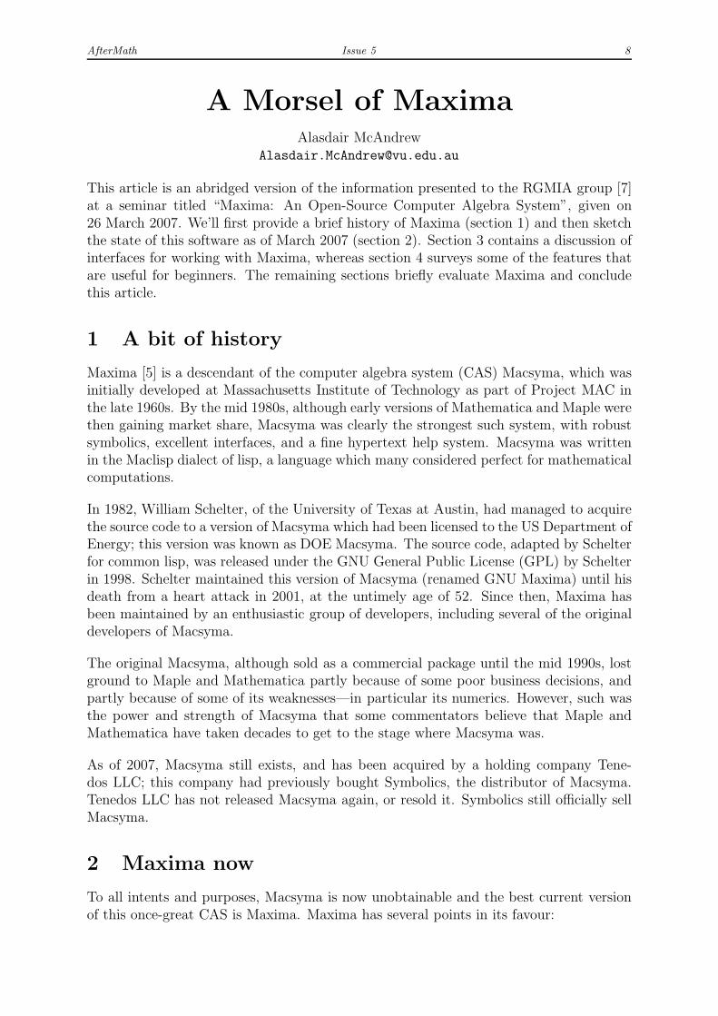
Figure 1 shows input and output taken from a window running Maxima in console mode.The result, typeset in ASCII, although readable, is not pleasant.

A slightly better interface, in that it allows cutting and pasting between commands,and incorporates a help browser, is Xmaxima, which comes standard with the software.

AfterMath Issue 5 10

Figure 1: Maxima running in console mode.

Xmaxima also allows included graphics and provides a sort of very cut-down windowinginterface.

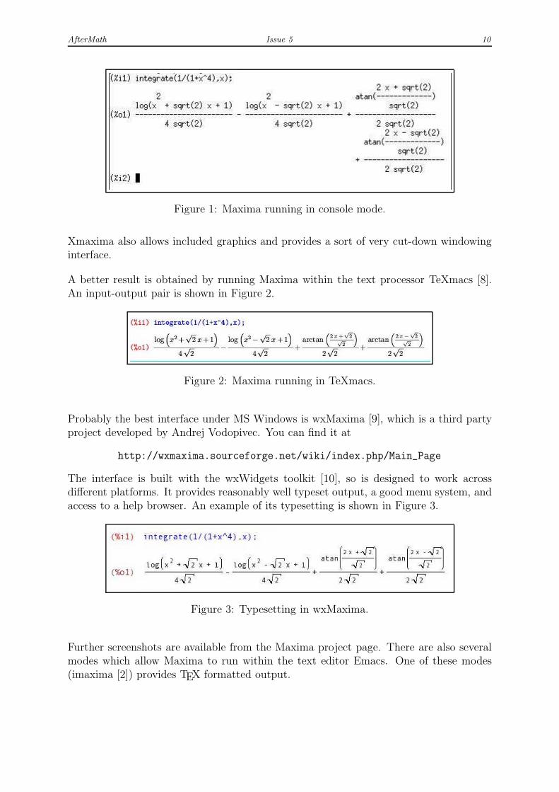
A better result is obtained by running Maxima within the text processor TeXmacs [8].An input-output pair is shown in Figure 2.

Figure 2: Maxima running in TeXmacs.

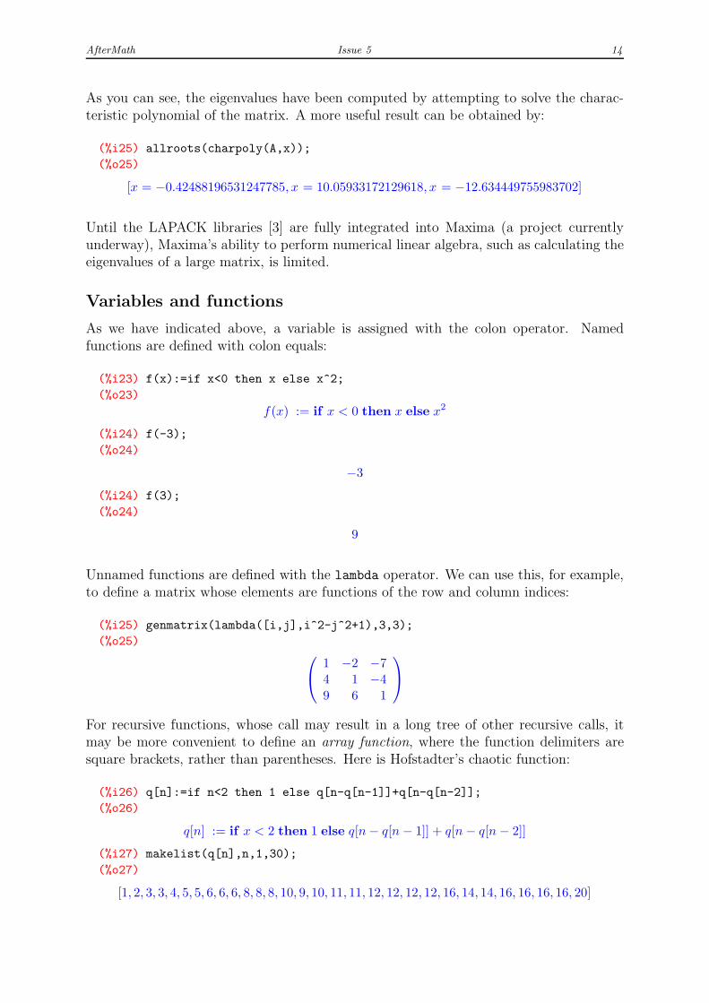
Probably the best interface under MS Windows is wxMaxima [9], which is a third partyproject developed by Andrej Vodopivec. You can find it at

http://wxmaxima.sourceforge.net/wiki/index.php/Main_Page

The interface is built with the wxWidgets toolkit [10], so is designed to work acrossdifferent platforms. It provides reasonably well typeset output, a good menu system, andaccess to a help browser. An example of its typesetting is shown in Figure 3.

Figure 3: Typesetting in wxMaxima.

Further screenshots are available from the Maxima project page. There are also severalmodes which allow Maxima to run within the text editor Emacs. One of these modes(imaxima [2]) provides TEX formatted output.


4 Some examples of Maxima in use

Arithmetic

Maxima can, as all good CASs can, perform arithmetic to arbitrary precision:

(%i3) sum(1/n,n,1,100);

(%o3)

14466636279520351160221518043104131447711

2788815009188499086581352357412492142272

(%i4) fpprec:80$

(%i5) bfloat(%pi);

(%o5)

3.141592653589793238462643383279502884197169399375105820974944592307816406286209b0

Polynomials and rational functions

We can expect the usual things: expansion and factorization, division with remainder,partial fractions. Maxima in fact has a suite of commands to enable efficient handlingof such expressions. For example, we can use factor to factor polynomials over a fieldextended by an element whose minimal polynomial is given:

(%i9) factor(x^4+1,a^2+2);

(%o9)

(x2 − ax− 1)(x2 + ax− 1)

And of course partial fractions:

(%i10) expand((x^3/(x^2+1))^4);

(%o10)

x12

x8 + 4x6 + 6x4 + 4x2 + 1

(%i11) partfrac(%,x);

(%o11)

− 20

x2 + 1+

15

(x2 + 1)2− 6

(x2 + 1)3+

1

(x2 + 1)4+ x4 − 4x2 + 10


Calculus

As you would expect, limits (directionless, or with a direction given), differentiation,integration, Taylor series:

(%i13) k(x):=(3*x-15)/(x^2-10*x+25)^(1/2);

(%o13)

k(x) :=3x− 15

(x2 − 10x + 25)1

2

(%i14) limit(k(x),x,5,plus);

(%o14)

3

(%i15) limit(k(x),x,5,minus);

(%o15)

−3

(%i12) diff(bessel_i(0,x),x,4)$

(%i13) radcan(%);

(%o13)

bessel i(4, x) + 4 bessel i(2, x) + 3 bessel i(0, x)

8

(%i14) integrate(1/(x^5+1),x);

(%o14)

(√

5− 3) log(2x2 + (√

5− 1)x + 2)

10− 10√

5− (√

5 + 3) log(2x2 + (−√

5− 1)x + 2)

10√

5 + 10

+

(√

5 + 1) arctan

(

4x+√

5−1√(2√

5+10)

)

√5√

(2√

5 + 10)+

(√

5− 1) arctan

(

4x−√

5−1√(10−2

√5)

)

(√

5√

(10 − 2√

5))+

log(x + 1)

5

(%i15) t:taylor(sqrt(x^2+1),x,0,10);

(%o15)

1 +x2

2− x4

8+

x6

16− 5x8

128+

7x10

256+ · · ·

(%i16) pade(t,6,6);

(%o16)

[

− 70x4 + 224x2 + 160

x6 − 18x4 − 144x2 − 160,x6 + 18x4 + 48x2 + 32

6x4 + 32x2 + 32

]


Linear algebra

We’ll create a few matrices and play with them:

(%i17) A:matrix([1,2,3],[4,5,6],[7,8,-9]);

(%o17)

1 2 34 5 67 8 −9

(%i18) B:matrix([1,-2,3],[-4,5,-6],[7,8,9]);

(%o18)

1 −2 3−4 5 −6

7 8 9

(%i19) A.B;

(%o19)

14 32 1826 65 36−88 −46 −108

(%i20) invert(A);

(%o20)

−3118

79 − 1

18

139 −5

919

− 118

19 − 1

18

(%i21) charpoly(B,alpha)$

(%i22) expand(%);

(%o22)

−α3 + 15α2 − 78α − 96

We can also compute eigenvalues:

(%i23) eigenvalues(A);

(%o24)

(

−(√

3 i)

/2− 1

2

) (

3√

8682 i− 37) 1

3

+43

((√3 i

)/2− 1

2

)

(3√

8682 i− 37) 1

3

− 1,

((√3 i

)

/2− 1

2

) (

3√

8682 i− 37) 1

3

+43

(−

(√3 i

)/2− 1

2

)

(3√

8682 i− 37) 1

3

− 1,

(

3√

8682 i− 37) 1

3

+ 43/

((

3√

8682 i− 37) 1

3

)

− 1

, [1, 1, 1]


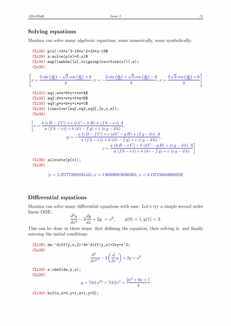
As you can see, the eigenvalues have been computed by attempting to solve the charac-teristic polynomial of the matrix. A more useful result can be obtained by:

(%i25) allroots(charpoly(A,x));

(%o25)

[x = −0.42488196531247785, x = 10.05933172129618, x = −12.634449755983702]

Until the LAPACK libraries [3] are fully integrated into Maxima (a project currentlyunderway), Maxima’s ability to perform numerical linear algebra, such as calculating theeigenvalues of a large matrix, is limited.

Variables and functions

As we have indicated above, a variable is assigned with the colon operator. Namedfunctions are defined with colon equals:

(%i23) f(x):=if x<0 then x else x^2;

(%o23)

f(x) := if x < 0 then x else x2

(%i24) f(-3);

(%o24)

−3

(%i24) f(3);

(%o24)

9

Unnamed functions are defined with the lambda operator. We can use this, for example,to define a matrix whose elements are functions of the row and column indices:

(%i25) genmatrix(lambda([i,j],i^2-j^2+1),3,3);

(%o25)

1 −2 −74 1 −49 6 1

For recursive functions, whose call may result in a long tree of other recursive calls, itmay be more convenient to define an array function, where the function delimiters aresquare brackets, rather than parentheses. Here is Hofstadter’s chaotic function:

(%i26) q[n]:=if n<2 then 1 else q[n-q[n-1]]+q[n-q[n-2]];

(%o26)

q[n] := if x < 2 then 1 else q[n− q[n− 1]] + q[n− q[n− 2]]

(%i27) makelist(q[n],n,1,30);

(%o27)

[1, 2, 3, 3, 4, 5, 5, 6, 6, 6, 8, 8, 8, 10, 9, 10, 11, 11, 12, 12, 12, 12, 16, 14, 14, 16, 16, 16, 16, 20]


Solving equations

Maxima can solve many algebraic equations, some numerically, some symbolically:

(%i28) p(x):=3*x^3-18*x^2+33*x-19$

(%i29) s:solve(p(x)=0,x)$

(%i30) map(lambda([x],trigsimp(rectform(x))),s);

(%o30)

[

x =3 sin

(π18

)−√

3 cos(π18

)+ 6

3, x = −3 sin

(π18

)+√

3 cos(π18

)− 6

3, x =

2√

3 cos(π18

)+ 6

3

]

(%i31) eq1:a*x+b*y+c*z=A$

(%i32) eq2:d*x+e*y+f*z=B$

(%i33) eq3:g*x+h*y+i*z=C$

(%i34) linsolve([eq1,eq2,eq3],[x,y,z]);

(%o34)

[

x =b (iB − f C) + c (eC − hB) + (f h− e i) A

a (f h− e i) + b (d i− f g) + c (e g − dh),

y = −a (iB − f C) + c (dC − g B) + (f g − d i) A

a (f h− e i) + b (d i− f g) + c (e g − dh),

z =a (hB − eC) + b (dC − g B) + (e g − dh) A

a (f h− e i) + b (d i− f g) + c (e g − dh)

]

(%i35) allroots(p(x));

(%o35)

[x = 1.257772801031441, x = 1.605069156365301, x = 3.137158042603259]

Differential equations

Maxima can solve many differential equations with ease. Let’s try a simple second orderlinear ODE:

d2y

dx2− 3

dy

dx+ 2y = x2, y(0) = 1, y(1) = 3.

This can be done in three steps: first defining the equation, then solving it, and finallyentering the initial conditions:

(%i28) de:’diff(y,x,2)-3*’diff(y,x)+2*y=x^2;

(%o28)

d2

dx2y − 3

(d

dxy

)

+ 2y = x2

(%i29) s:ode2(de,y,x);

(%o29)

y = %k1 e2x + %k2 ex +2x2 + 6x + 7

4

(%i30) bc2(s,x=0,y=1,x=1,y=3);


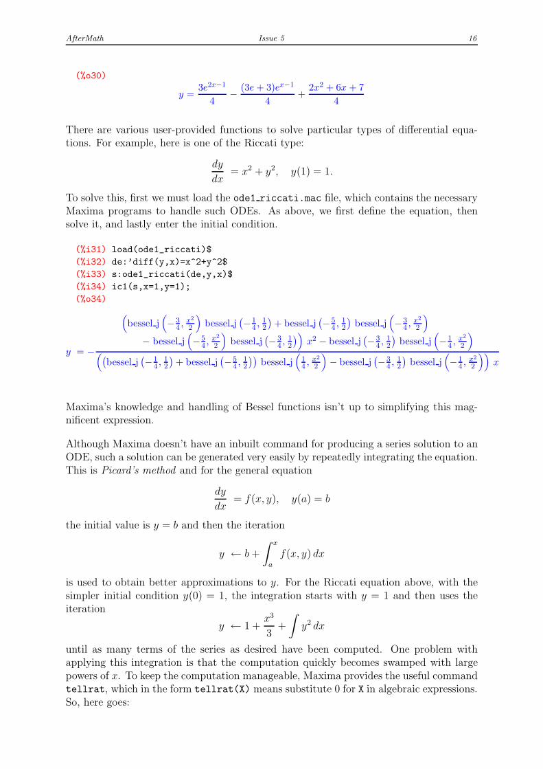
(%o30)

y =3e2x−1

4− (3e + 3)ex−1

4+

2x2 + 6x + 7

4

There are various user-provided functions to solve particular types of differential equa-tions. For example, here is one of the Riccati type:

dy

dx= x2 + y2, y(1) = 1.

To solve this, first we must load the ode1 riccati.mac file, which contains the necessaryMaxima programs to handle such ODEs. As above, we first define the equation, thensolve it, and lastly enter the initial condition.

(%i31) load(ode1_riccati)$

(%i32) de:’diff(y,x)=x^2+y^2$

(%i33) s:ode1_riccati(de,y,x)$

(%i34) ic1(s,x=1,y=1);

(%o34)

y = −

(

bessel j(

−34 , x

2

2

)

bessel j(−1

4 , 12

)+ bessel j

(−5

4 , 12

)bessel j

(

−34 , x

2

2

)

− bessel j(

−54 , x

2

2

)

bessel j(−3

4 , 12

))

x2 − bessel j(−3

4 , 12

)bessel j

(

−14 , x

2

2

)

((bessel j

(−1

4 , 12

)+ bessel j

(−5

4 , 12

))bessel j

(14 , x

2

2

)

− bessel j(−3

4 , 12

)bessel j

(

−14 , x

2

2

))

x

Maxima’s knowledge and handling of Bessel functions isn’t up to simplifying this mag-nificent expression.

Although Maxima doesn’t have an inbuilt command for producing a series solution to anODE, such a solution can be generated very easily by repeatedly integrating the equation.This is Picard’s method and for the general equation

dy

dx= f(x, y), y(a) = b

the initial value is y = b and then the iteration

y ← b+

∫ x

a

f(x, y) dx

is used to obtain better approximations to y. For the Riccati equation above, with thesimpler initial condition y(0) = 1, the integration starts with y = 1 and then uses theiteration

y ← 1 +x3

3+

∫

y2 dx

until as many terms of the series as desired have been computed. One problem withapplying this integration is that the computation quickly becomes swamped with largepowers of x. To keep the computation manageable, Maxima provides the useful commandtellrat, which in the form tellrat(X) means substitute 0 for X in algebraic expressions.So, here goes:


(%i35) tellrat(x^11)$

(%i36) algebraic:true$

(%i37) for i : 1 thru 12 do y : rat(1+x^3/3+integrate(y^2,x))$

(%i38) expand(y);

(%o38)

1961x10

1400+

428x9

315+

369x8

280+

404x7

315+

37x6

30+

6x5

5+

7x4

6+

4x3

3+ x2 + x + 1

Plotting

Maxima’s plotting is based on the Gnuplot [1] software, which allows for plotting of twoand three dimensional functions, and datasets. So a plot2d or plot3d command collectsthe functions and parameters, and passes them all to Gnuplot for plotting. Gnuplot isbundled with Maxima, so there is no need to install it separately.

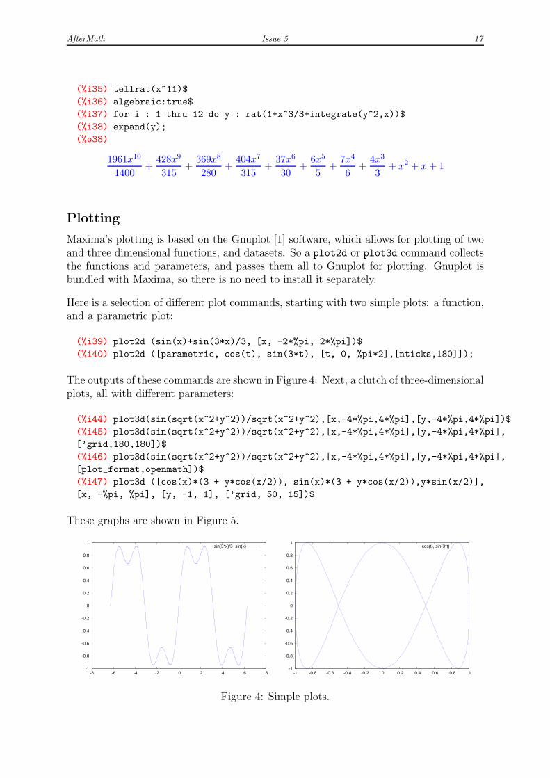
Here is a selection of different plot commands, starting with two simple plots: a function,and a parametric plot:

(%i39) plot2d (sin(x)+sin(3*x)/3, [x, -2*%pi, 2*%pi])$

(%i40) plot2d ([parametric, cos(t), sin(3*t), [t, 0, %pi*2],[nticks,180]]);

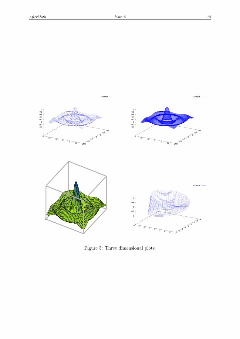
The outputs of these commands are shown in Figure 4. Next, a clutch of three-dimensionalplots, all with different parameters:

(%i44) plot3d(sin(sqrt(x^2+y^2))/sqrt(x^2+y^2),[x,-4*%pi,4*%pi],[y,-4*%pi,4*%pi])$

(%i45) plot3d(sin(sqrt(x^2+y^2))/sqrt(x^2+y^2),[x,-4*%pi,4*%pi],[y,-4*%pi,4*%pi],

[’grid,180,180])$

(%i46) plot3d(sin(sqrt(x^2+y^2))/sqrt(x^2+y^2),[x,-4*%pi,4*%pi],[y,-4*%pi,4*%pi],

[plot_format,openmath])$

(%i47) plot3d ([cos(x)*(3 + y*cos(x/2)), sin(x)*(3 + y*cos(x/2)),y*sin(x/2)],

[x, -%pi, %pi], [y, -1, 1], [’grid, 50, 15])$

These graphs are shown in Figure 5.

-1

-0.8

-0.6

-0.4

-0.2

0

0.2

0.4

0.6

0.8

1

-8 -6 -4 -2 0 2 4 6 8

sin(3*x)/3+sin(x)

-1

-0.8

-0.6

-0.4

-0.2

0

0.2

0.4

0.6

0.8

1

-1 -0.8 -0.6 -0.4 -0.2 0 0.2 0.4 0.6 0.8 1

cos(t), sin(3*t)

Figure 4: Simple plots.


-15-10

-5 0

5 10

15-15-10

-5 0

5 10

15

-0.4-0.2

0 0.2 0.4 0.6 0.8

1

Function

-15-10

-5 0

5 10

15-15-10

-5 0

5 10

15

-0.4-0.2

0 0.2 0.4 0.6 0.8

1

Function

-4 -3 -2 -1 0 1 2 3 4-4-3

-2-1

0 1

2 3

4

-1

-0.5

0

0.5

1

Function

Figure 5: Three dimensional plots.


5 Help and documentation

Plenty of help is provided. Its main fault is that it is not properly typeset: all themathematical material is presented as ASCII. Here, for example, is a snippet from thehelp section on integration:

(%i1) assume(a > 0)$

(%i2) ’integrate (%e**sqrt(a*y), y, 0, 4);

4

/

[ sqrt(a) sqrt(y)

(%o2) I %e dy

]

/

0

The advantage of using ASCII though, means that Maxima’s help can be read on manysystems and interfaces, from plain console mode to a PDF file (in which the math stillappears as ASCII). So a loss, possibly, of typesetting elegance may be compensatedby flexibility. Many users, however, will consider the slightly clunky appearance as anegative.

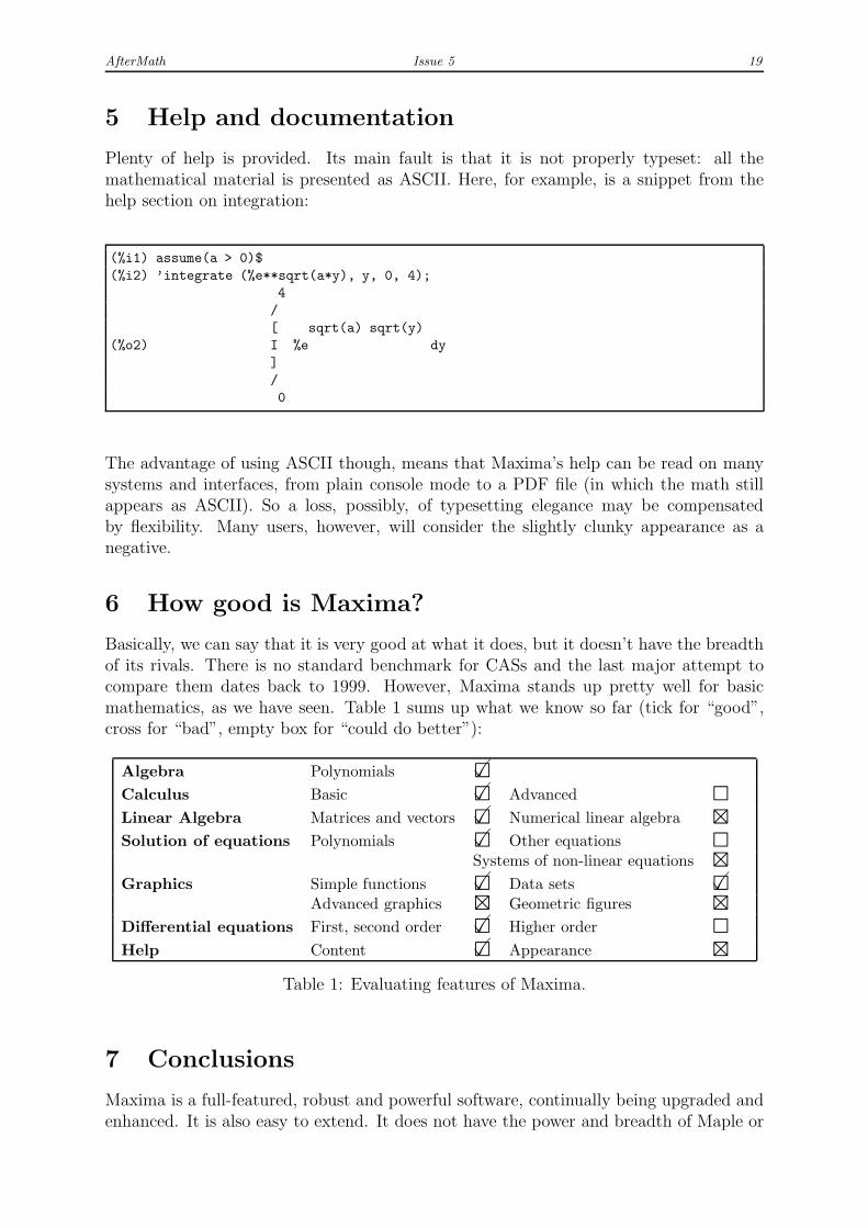
6 How good is Maxima?

Basically, we can say that it is very good at what it does, but it doesn’t have the breadthof its rivals. There is no standard benchmark for CASs and the last major attempt tocompare them dates back to 1999. However, Maxima stands up pretty well for basicmathematics, as we have seen. Table 1 sums up what we know so far (tick for “good”,cross for “bad”, empty box for “could do better”):

Algebra Polynomials 2�

Calculus Basic 2� Advanced 2

Linear Algebra Matrices and vectors 2� Numerical linear algebra 4

Solution of equations Polynomials 2� Other equations 2Systems of non-linear equations 4

Graphics Simple functions 2� Data sets 2�Advanced graphics 4 Geometric figures 4

Differential equations First, second order 2� Higher order 2

Help Content 2� Appearance 4

Table 1: Evaluating features of Maxima.

7 Conclusions

Maxima is a full-featured, robust and powerful software, continually being upgraded andenhanced. It is also easy to extend. It does not have the power and breadth of Maple or


Mathematica (yet!), but it is a very clean system, elegantly programmed, and of courseavailable on many platforms—even online [6]. As to whether Maxima will suit your needs,the only way to find out is to test it: download it, play with it, investigate it.

Over to you!

References

[1] Gnuplot Team. Gnuplot (version 4.2.3), 10 September 2008.http://www.gnuplot.info.

[2] Y. Honda. Imaxima: GUI for Maxima/Macsyma computer algebra system in Emacs (ver-sion 1.0b), 10 September 2008.http://members3.jcom.home.ne.jp/imaxima/Site/Welcome.html.

[3] LAPACK Team. LAPACK – Linear Algebra PACKage (version 3.1.1), 10 September 2008.http://www.netlib.org/lapack.

[4] Maxima. Maxima mailing list, 09 September [email protected]

http://www.math.utexas.edu/mailman/listinfo/maxima.[5] Maxima. Maxima (version 5.16.3), 09 September 2008.

http://maxima.sourceforge.net.[6] MaximaPHP. MaximaPHP – Maxima online, 10 September 2008.

http://www.my-tool.com/mathematics/maximaphp.[7] RGMIA. Research group in mathematical inequalities and applications, 10 September

2008.http://www.staff.vu.edu.au/rgmia.

[8] J. van der Hoeven. GNU TeXmacs: a WYSIWIG technical editor (version 1.0.6),10 September 2008.http://www.texmacs.org.

[9] A. Vodopivec. wxMaxima (version 0.7.6), 10 September 2008.http://wxmaxima.sourceforge.net/wiki/index.php/Main_Page.

[10] wxWidgets Team. wxWidgets cross-platform GUI library (version 2.8.8), 10 September2008.http://www.wxwidgets.org.


Number Theory and Cryptographyusing PARI/GP

Minh Van [email protected]

This article uses PARI/GP to study elementary number theory and the RSA publickey cryptosystem. Various PARI/GP commands will be introduced that can help us toperform basic number theoretic operations such as greatest common divisor and Euler’sphi function. We then introduce the RSA cryptosystem and use PARI/GP’s built-incommands to encrypt and decrypt data via the RSA algorithm. It should be noted thatour brief exposition on RSA and cryptography is for educational purposes only. Readerswho require further detailed discussions are encouraged to consult specialized texts suchas [2, 5, 6].

1 What is PARI/GP?

PARI/GP [3] is a computer algebra system that is geared towards research in numbertheory. It can be used as a powerful desktop calculator, as a tool to help undergraduatestudents study number theory, or as a programming environment for studying numbertheoretic cryptosystems. PARI/GP is available free of charge and can be downloadedfrom the following website:

http://pari.math.u-bordeaux.fr

The default interface to PARI/GP is command line based, but there are graphical userinterfaces to the software as well. Figure 6 shows sample PARI/GP sessions under Linuxand Windows.

2 Elementary number theory

This section reviews basic concepts from elementary number theory, including the notionof primes, greatest common divisors, congruences and Euler’s phi function. The num-ber theoretic concepts and PARI/GP commands introduced will be referred to in latersections when we present the RSA algorithm.

Prime numbers

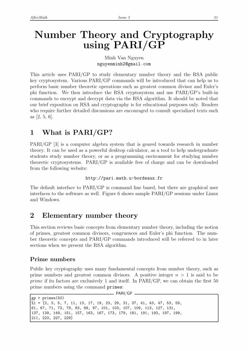
Public key cryptography uses many fundamental concepts from number theory, such asprime numbers and greatest common divisors. A positive integer n > 1 is said to beprime if its factors are exclusively 1 and itself. In PARI/GP, we can obtain the first 50prime numbers using the command primes:

PARI/GPgp > primes(50)

%1 = [2, 3, 5, 7, 11, 13, 17, 19, 23, 29, 31, 37, 41, 43, 47, 53, 59,

61, 67, 71, 73, 79, 83, 89, 97, 101, 103, 107, 109, 113, 127, 131,

137, 139, 149, 151, 157, 163, 167, 173, 179, 181, 191, 193, 197, 199,

211, 223, 227, 229]


Figure 6: PARI/GP sessions under Linux (top) and Windows (bottom).


Greatest common divisors

Let Z be the set of integers. If a, b ∈ Z, then the greatest common divisor (GCD) of aand b is the largest positive factor of both a and b. We use gcd(a, b) to denote this largestpositive factor. The GCD of any two distinct primes is 1, and the GCD of 18 and 27 is9. We can use the command gcd to compute the GCD of any two integers:

PARI/GPgp > gcd(3, 59)

%2 = 1

gp > gcd(18, 27)

%3 = 9

If gcd(a, b) = 1, we say that a is coprime (or relatively prime) to b. In particular,gcd(3, 59) = 1 so 3 is coprime to 59.

Congruences

When one integer is divided by a non-zero integer, we usually get a remainder. Forexample, upon dividing 23 by 5, we get a remainder of 3; when 8 is divided by 5, theremainder is again 3. The notion of congruence helps us to describe the situation in whichtwo integers have the same remainder upon division by a non-zero integer. Let a, b, n ∈ Z

such that n 6= 0. If a and b have the same remainder upon division by n, then we saythat a is congruent to b modulo n and denote this relationship by

a ≡ b (mod n)

This definition is equivalent to saying that n divides the difference of a and b, that is,n | (a− b). Thus 23 ≡ 8 (mod 5) because when both 23 and 8 are divided by 5, we endup with a remainder of 3. The command Mod allows us to compute such a remainder:

PARI/GPgp > Mod(23, 5)

%4 = Mod(3, 5)

gp > Mod(8, 5)

%5 = Mod(3, 5)

Euler’s phi function

Consider all the integers from 1 to 20, inclusive. List all those integers that are coprimeto 20. In other words, we want to find those integers n, where 1 ≤ n ≤ 20, suchthat gcd(n, 20) = 1. The latter task can be easily accomplished with some PARI/GPprogramming:

PARI/GPgp > for (n = 1, 20, if (gcd(n,20) == 1, print1(n, " ")))

1 3 7 9 11 13 17 19

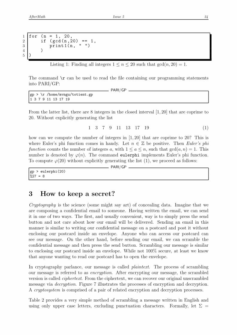
The above programming statement can be saved into a text file named, for example,/home/mvngu/totient.gp, organizing it as in Listing 1 to enhance readability.


1 for (n = 1, 20,2 if (gcd(n,20) == 1,3 print1(n, " ")4 )5 )

Listing 1: Finding all integers 1 ≤ n ≤ 20 such that gcd(n, 20) = 1.

The command \r can be used to read the file containing our programming statementsinto PARI/GP:

PARI/GPgp > \r /home/mvngu/totient.gp

1 3 7 9 11 13 17 19

From the latter list, there are 8 integers in the closed interval [1, 20] that are coprime to20. Without explicitly generating the list

1 3 7 9 11 13 17 19 (1)

how can we compute the number of integers in [1, 20] that are coprime to 20? This iswhere Euler’s phi function comes in handy. Let n ∈ Z be positive. Then Euler’s phifunction counts the number of integers a, with 1 ≤ a ≤ n, such that gcd(a, n) = 1. Thisnumber is denoted by ϕ(n). The command eulerphi implements Euler’s phi function.To compute ϕ(20) without explicitly generating the list (1), we proceed as follows:

PARI/GPgp > eulerphi(20)

%27 = 8

3 How to keep a secret?

Cryptography is the science (some might say art) of concealing data. Imagine that weare composing a confidential email to someone. Having written the email, we can sendit in one of two ways. The first, and usually convenient, way is to simply press the sendbutton and not care about how our email will be delivered. Sending an email in thismanner is similar to writing our confidential message on a postcard and post it withoutenclosing our postcard inside an envelope. Anyone who can access our postcard cansee our message. On the other hand, before sending our email, we can scramble theconfidential message and then press the send button. Scrambling our message is similarto enclosing our postcard inside an envelope. While not 100% secure, at least we knowthat anyone wanting to read our postcard has to open the envelope.

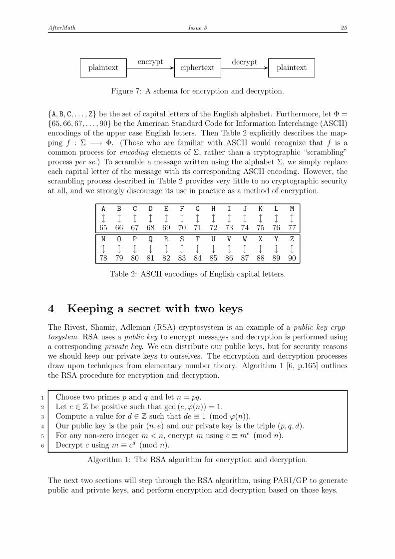
In cryptography parlance, our message is called plaintext. The process of scramblingour message is referred to as encryption. After encrypting our message, the scrambledversion is called ciphertext. From the ciphertext, we can recover our original unscrambledmessage via decryption. Figure 7 illustrates the processes of encryption and decryption.A cryptosystem is comprised of a pair of related encryption and decryption processes.

Table 2 provides a very simple method of scrambling a message written in English andusing only upper case letters, excluding punctuation characters. Formally, let Σ =


plaintext ciphertext plaintextencrypt decrypt

Figure 7: A schema for encryption and decryption.

{A, B, C, . . . , Z} be the set of capital letters of the English alphabet. Furthermore, let Φ ={65, 66, 67, . . . , 90} be the American Standard Code for Information Interchange (ASCII)encodings of the upper case English letters. Then Table 2 explicitly describes the map-ping f : Σ −→ Φ. (Those who are familiar with ASCII would recognize that f is acommon process for encoding elements of Σ, rather than a cryptographic “scrambling”process per se.) To scramble a message written using the alphabet Σ, we simply replaceeach capital letter of the message with its corresponding ASCII encoding. However, thescrambling process described in Table 2 provides very little to no cryptographic securityat all, and we strongly discourage its use in practice as a method of encryption.

A B C D E F G H I J K L M

l l l l l l l l l l l l l65 66 67 68 69 70 71 72 73 74 75 76 77

N O P Q R S T U V W X Y Z

l l l l l l l l l l l l l78 79 80 81 82 83 84 85 86 87 88 89 90

Table 2: ASCII encodings of English capital letters.

4 Keeping a secret with two keys

The Rivest, Shamir, Adleman (RSA) cryptosystem is an example of a public key cryp-tosystem. RSA uses a public key to encrypt messages and decryption is performed usinga corresponding private key. We can distribute our public keys, but for security reasonswe should keep our private keys to ourselves. The encryption and decryption processesdraw upon techniques from elementary number theory. Algorithm 1 [6, p.165] outlinesthe RSA procedure for encryption and decryption.

Choose two primes p and q and let n = pq.1

Let e ∈ Z be positive such that gcd (e, ϕ(n)) = 1.2

Compute a value for d ∈ Z such that de ≡ 1 (mod ϕ(n)).3

Our public key is the pair (n, e) and our private key is the triple (p, q, d).4

For any non-zero integer m < n, encrypt m using c ≡ me (mod n).5

Decrypt c using m ≡ cd (mod n).6

Algorithm 1: The RSA algorithm for encryption and decryption.

The next two sections will step through the RSA algorithm, using PARI/GP to generatepublic and private keys, and perform encryption and decryption based on those keys.


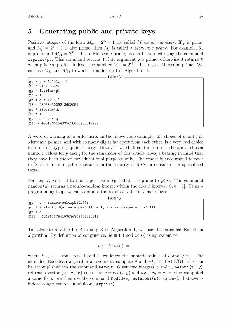
5 Generating public and private keys

Positive integers of the form Mm = 2m − 1 are called Mersenne numbers. If p is primeand Mp = 2p − 1 is also prime, then Mp is called a Mersenne prime. For example, 31is prime and M31 = 231 − 1 is a Mersenne prime, as can be verified using the commandisprime(p). This command returns 1 if its argument p is prime; otherwise it returns 0

when p is composite. Indeed, the number M61 = 261 − 1 is also a Mersenne prime. Wecan use M31 and M61 to work through step 1 in Algorithm 1:

PARI/GPgp > p = (2^31) - 1

%6 = 2147483647

gp > isprime(p)

%7 = 1

gp > q = (2^61) - 1

%8 = 2305843009213693951

gp > isprime(q)

%9 = 1

gp > n = p * q

%10 = 4951760154835678088235319297

A word of warning is in order here. In the above code example, the choice of p and q asMersenne primes, and with so many digits far apart from each other, is a very bad choicein terms of cryptographic security. However, we shall continue to use the above chosennumeric values for p and q for the remainder of this article, always bearing in mind thatthey have been chosen for educational purposes only. The reader is encouraged to referto [2, 5, 6] for in-depth discussions on the security of RSA, or consult other specializedtexts.

For step 2, we need to find a positive integer that is coprime to ϕ(n). The commandrandom(n) returns a pseudo-random integer within the closed interval [0, n− 1]. Using aprogramming loop, we can compute the required value of e as follows:

PARI/GPgp > e = random(eulerphi(n));

gp > while (gcd(e, eulerphi(n)) != 1, e = random(eulerphi(n)))

gp > e

%12 = 4048613754158036308925952619

To calculate a value for d in step 3 of Algorithm 1, we use the extended Euclideanalgorithm. By definition of congruence, de ≡ 1 (mod ϕ(n)) is equivalent to

de− k · ϕ(n) = 1

where k ∈ Z. From steps 1 and 2, we know the numeric values of e and ϕ(n). Theextended Euclidean algorithm allows us to compute d and −k. In PARI/GP, this canbe accomplished via the command bezout. Given two integers x and y, bezout(x, y)

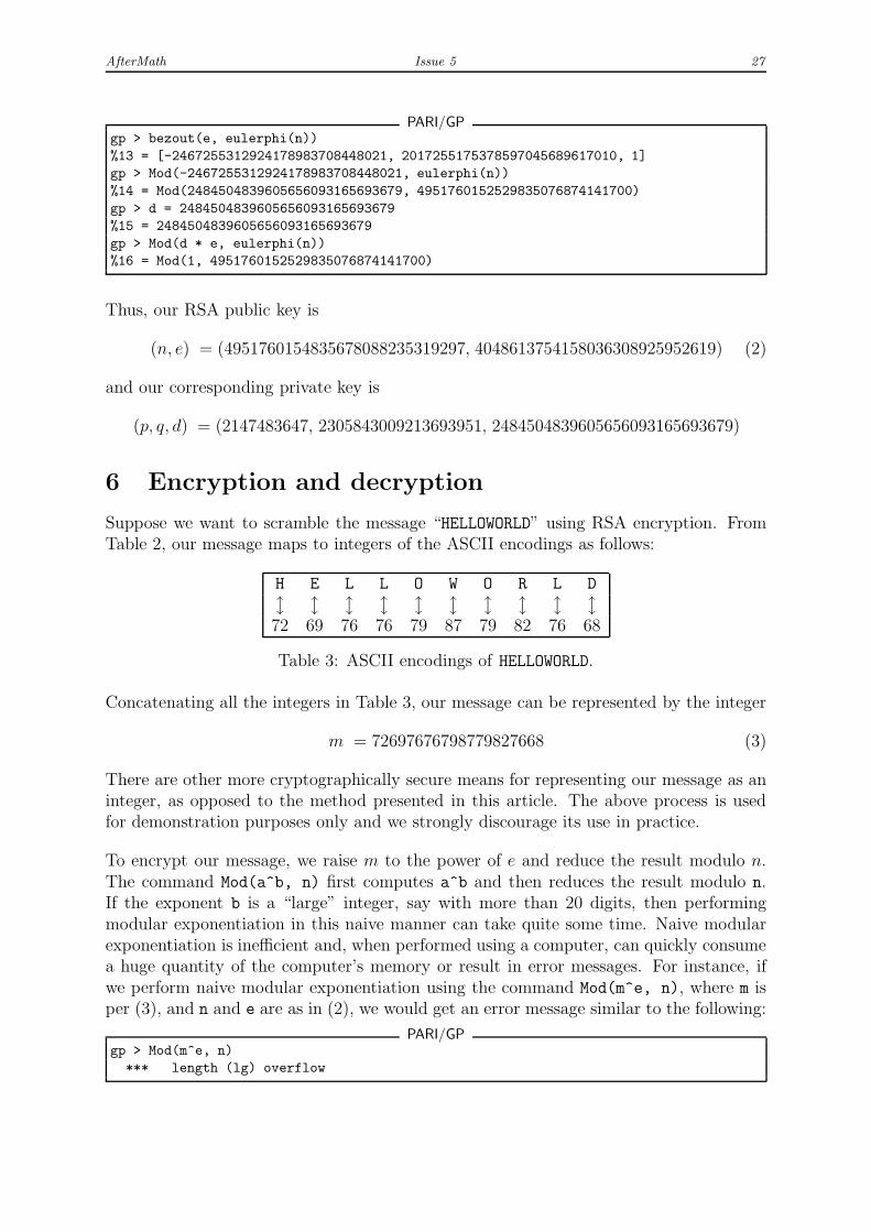
returns a vector [u, v, g] such that g = gcd(x, y) and ux+ vy = g. Having computeda value for d, we then use the command Mod(d*e, eulerphi(n)) to check that d*e isindeed congruent to 1 modulo eulerphi(n):


PARI/GPgp > bezout(e, eulerphi(n))

%13 = [-2467255312924178983708448021, 2017255175378597045689617010, 1]

gp > Mod(-2467255312924178983708448021, eulerphi(n))

%14 = Mod(2484504839605656093165693679, 4951760152529835076874141700)

gp > d = 2484504839605656093165693679

%15 = 2484504839605656093165693679

gp > Mod(d * e, eulerphi(n))

%16 = Mod(1, 4951760152529835076874141700)

Thus, our RSA public key is

(n, e) = (4951760154835678088235319297, 4048613754158036308925952619) (2)

and our corresponding private key is

(p, q, d) = (2147483647, 2305843009213693951, 2484504839605656093165693679)

6 Encryption and decryption

Suppose we want to scramble the message “HELLOWORLD” using RSA encryption. FromTable 2, our message maps to integers of the ASCII encodings as follows:

H E L L O W O R L D

l l l l l l l l l l72 69 76 76 79 87 79 82 76 68

Table 3: ASCII encodings of HELLOWORLD.

Concatenating all the integers in Table 3, our message can be represented by the integer

m = 72697676798779827668 (3)

There are other more cryptographically secure means for representing our message as aninteger, as opposed to the method presented in this article. The above process is usedfor demonstration purposes only and we strongly discourage its use in practice.

To encrypt our message, we raise m to the power of e and reduce the result modulo n.The command Mod(a^b, n) first computes a^b and then reduces the result modulo n.If the exponent b is a “large” integer, say with more than 20 digits, then performingmodular exponentiation in this naive manner can take quite some time. Naive modularexponentiation is inefficient and, when performed using a computer, can quickly consumea huge quantity of the computer’s memory or result in error messages. For instance, ifwe perform naive modular exponentiation using the command Mod(m^e, n), where m isper (3), and n and e are as in (2), we would get an error message similar to the following:

PARI/GPgp > Mod(m^e, n)

*** length (lg) overflow


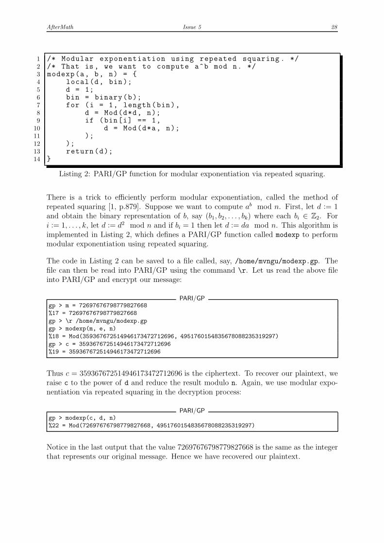
1 /* Modular exponentiation using repeated squaring . */2 /* That is , we want to compute a^b mod n. */3 modexp(a, b, n) = {4 local(d, bin);5 d = 1;6 bin = binary(b);7 for (i = 1, length(bin),8 d = Mod(d*d, n);9 if (bin[i] == 1,

10 d = Mod(d*a, n);11 );12 );13 return(d);14 }

Listing 2: PARI/GP function for modular exponentiation via repeated squaring.

There is a trick to efficiently perform modular exponentiation, called the method ofrepeated squaring [1, p.879]. Suppose we want to compute ab mod n. First, let d := 1and obtain the binary representation of b, say (b1, b2, . . . , bk) where each bi ∈ Z2. Fori := 1, . . . , k, let d := d2 mod n and if bi = 1 then let d := da mod n. This algorithm isimplemented in Listing 2, which defines a PARI/GP function called modexp to performmodular exponentiation using repeated squaring.

The code in Listing 2 can be saved to a file called, say, /home/mvngu/modexp.gp. Thefile can then be read into PARI/GP using the command \r. Let us read the above fileinto PARI/GP and encrypt our message:

PARI/GPgp > m = 72697676798779827668

%17 = 72697676798779827668

gp > \r /home/mvngu/modexp.gp

gp > modexp(m, e, n)

%18 = Mod(359367672514946173472712696, 4951760154835678088235319297)

gp > c = 359367672514946173472712696

%19 = 359367672514946173472712696

Thus c = 359367672514946173472712696 is the ciphertext. To recover our plaintext, weraise c to the power of d and reduce the result modulo n. Again, we use modular expo-nentiation via repeated squaring in the decryption process:

PARI/GPgp > modexp(c, d, n)

%22 = Mod(72697676798779827668, 4951760154835678088235319297)

Notice in the last output that the value 72697676798779827668 is the same as the integerthat represents our original message. Hence we have recovered our plaintext.


7 What’s next?

This article has demonstrated that the computer algebra system PARI/GP can be usedto study undergraduate number theory and cryptography. As the reader delves furtherinto number theory or its application to cryptography, software tools such as PARI/GPwould be handy in the learning process. Further information about PARI/GP can beobtained from its website at http://pari.math.u-bordeaux.fr.

The structure of this article closely follows the tutorial Number Theory and the RSAPublic Key Cryptosystem, written by the same author for the Sage [4] documentationproject. That tutorial can be found online at

http://wiki.sagemath.org/DocumentationProject

Many of the invaluable feedbacks by Martin Albrecht and William Stein to that tutorialhave been incorporated into this article.

References

[1] T. H. Cormen, C. E. Leiserson, R. L. Rivest, and C. Stein. Introduction to Algorithms. TheMIT Press, USA, 2nd edition, 2001.

[2] A. J. Menezes, P. C. van Oorschot, and S. A. Vanstone. Handbook of Applied Cryptography.CRC Press, Boca Raton, FL, USA, 1996.

[3] PARI Group. PARI/GP (version 2.3.4), July 2008.http://pari.math.u-bordeaux.fr.

[4] W. Stein. Sage: Open Source Mathematics Software (version 3.1.4). The Sage Group,03 November 2008.http://www.sagemath.org.

[5] D. R. Stinson. Cryptography: Theory and Practice. Chapman & Hall/CRC, Boca Raton,USA, 3rd edition, 2006.

[6] W. Trappe and L. C. Washington. Introduction to Cryptography with Coding Theory. Pear-son Prentice Hall, Upper Saddle River, New Jersey, USA, 2nd edition, 2006.


Jokes Corner• 2 lemmas = 1 dilemma

• A digraph is a directed graph. A dilemma is a directed lemma.

• Polytheist: There are many gods.Monotheist: There is only one god.Mathematician: There’s only one god up to isomorphism.

• Introduction to graph theory.Definition 1: A dag is a directed acyclic graph.Definition 2: A dagger is a dag with sharp edges.

• There are Lie groups, Lie algebras, and there’s statistics.


Problems Section1. It is a well known fact that 0.999 . . . :=

∞∑

i=0

(0.9)10−i = 0.91−10−1 = 1. Show by

induction that 0. 999 . . .9︸︷︷︸

n times

< 1. Why does this not contradict 0.999 . . . = 1?

2. Show that√

2 is irrational by assuming√

2 = p

q(where p, q have only 1 as a common

factor) and deriving a contradiction.

3. Show that an irrational number raised to the power of an irrational number is notnecessarily irrational. Hint: Use the result of the previous question.

aftermath issue 5 1 - university of western...

Documents