Northwestern University Prosthetics-Orthotics Center

AFO 3D: User's Manual

Kerice-Ahmun Tucker 2013

680 N. Lake Shore Drive, Suite 1100 Chicago, IL 60611

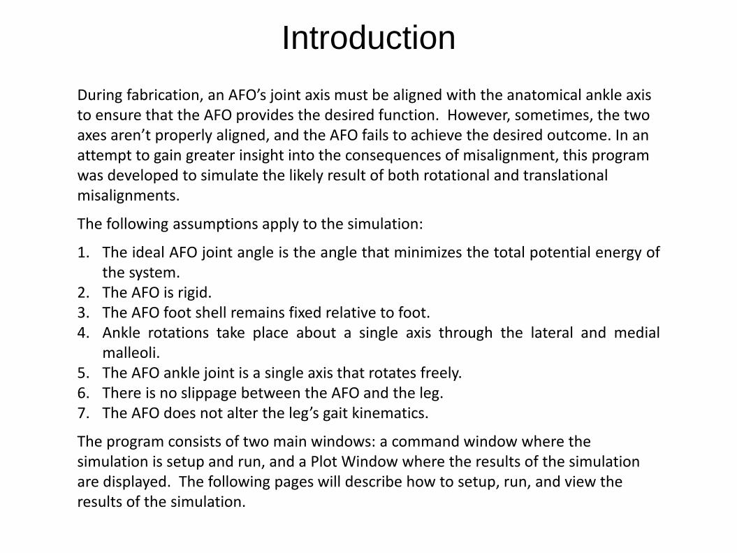
During fabrication, an AFO’s joint axis must be aligned with the anatomical ankle axis to ensure that the AFO provides the desired function. However, sometimes, the two axes aren’t properly aligned, and the AFO fails to achieve the desired outcome. In an attempt to gain greater insight into the consequences of misalignment, this program was developed to simulate the likely result of both rotational and translational misalignments.

The following assumptions apply to the simulation:

1. The ideal AFO joint angle is the angle that minimizes the total potential energy of the system.

2. The AFO is rigid. 3. The AFO foot shell remains fixed relative to foot. 4. Ankle rotations take place about a single axis through the lateral and medial

malleoli. 5. The AFO ankle joint is a single axis that rotates freely. 6. There is no slippage between the AFO and the leg. 7. The AFO does not alter the leg’s gait kinematics.

The program consists of two main windows: a command window where the simulation is setup and run, and a Plot Window where the results of the simulation are displayed. The following pages will describe how to setup, run, and view the results of the simulation.

Introduction

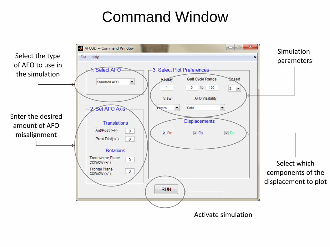
Select the type of AFO to use in the simulation

Enter the desired amount of AFO misalignment

Select which components of the

displacement to plot

Simulation parameters

Activate simulation

Command Window

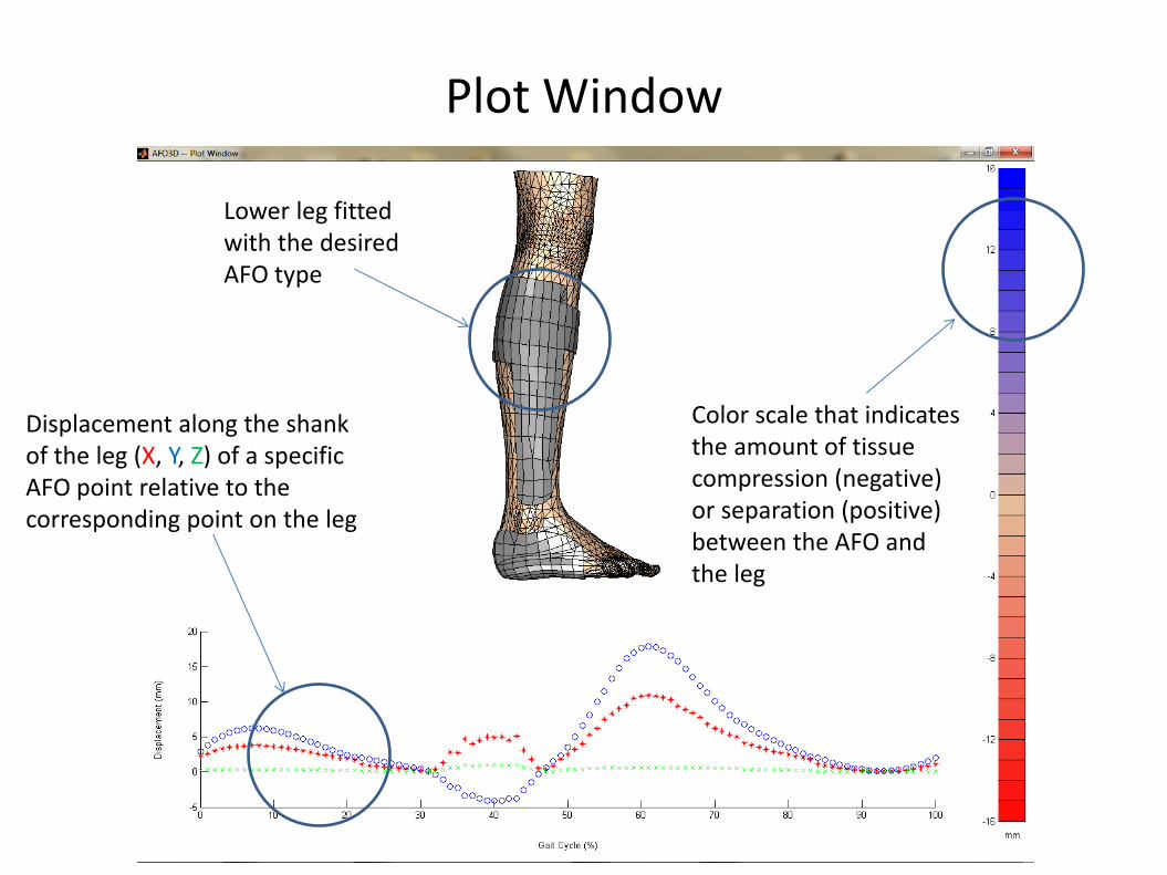
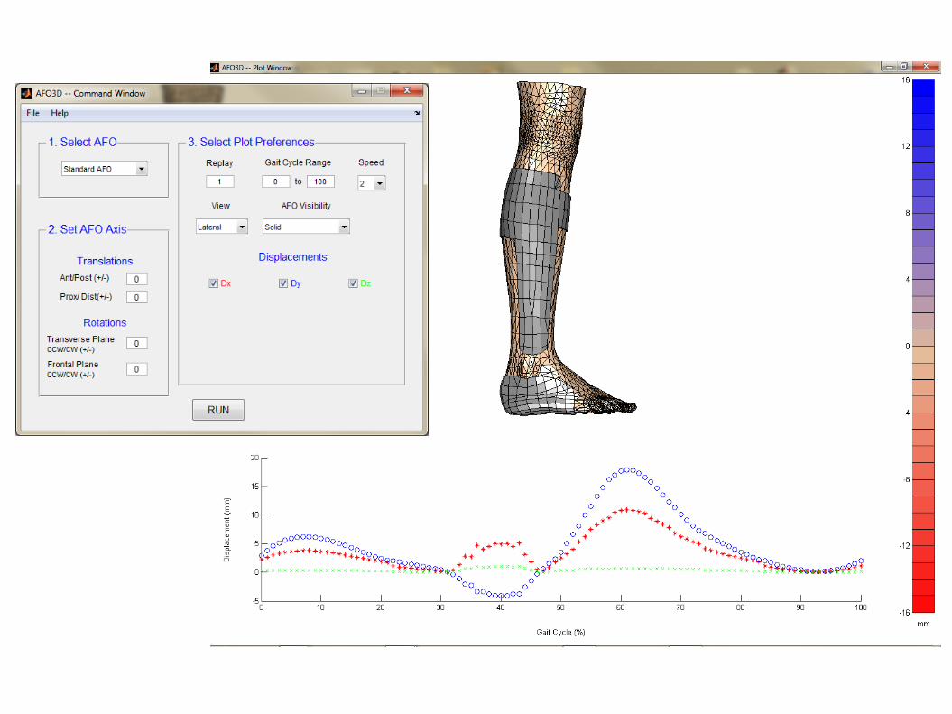
Displacement along the shank of the leg (X, Y, Z) of a specific AFO point relative to the corresponding point on the leg

Color scale that indicates the amount of tissue compression (negative) or separation (positive) between the AFO and the leg

Lower leg fitted with the desired AFO type

Plot Window

The Command Window is divided into three sections: Select AFO, Set AFO Axis, and Select Plot Preferences.

1. Select AFO

This drop-down menu item provides access to the available AFO types that can be run in the simulation. Click the down arrow in the right corner to display all types.

Note: The simulation must be run (press ‘Run’ button) prior to viewing the AFO from different views.

Available Styles: Standard AFO, Open Achilles AFO, AFO with Lateral Flange, PTB Height Bivalve AFO, and Conventional AFO

2. Set AFO Axis

This section allows the user to define the desired AFO joint axis misalignment. Both translations and rotations are available. Translations are restricted to the sagittal plane, and rotations are only available in the transverse and coronal planes. Slides #6-9 define the directions of translation and rotation.

Initially, the AFO axis and anatomical ankle axis are coincident. Any misalignments are defined relative to the anatomical ankle axis.

The maximum input for all fields is +/- 20. Units: translations – millimeters; rotations -degrees.

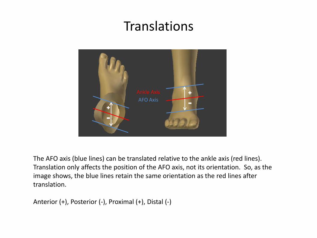
Translations

Ankle Axis

AFO Axis

The AFO axis (blue lines) can be translated relative to the ankle axis (red lines). Translation only affects the position of the AFO axis, not its orientation. So, as the image shows, the blue lines retain the same orientation as the red lines after translation. Anterior (+), Posterior (-), Proximal (+), Distal (-)

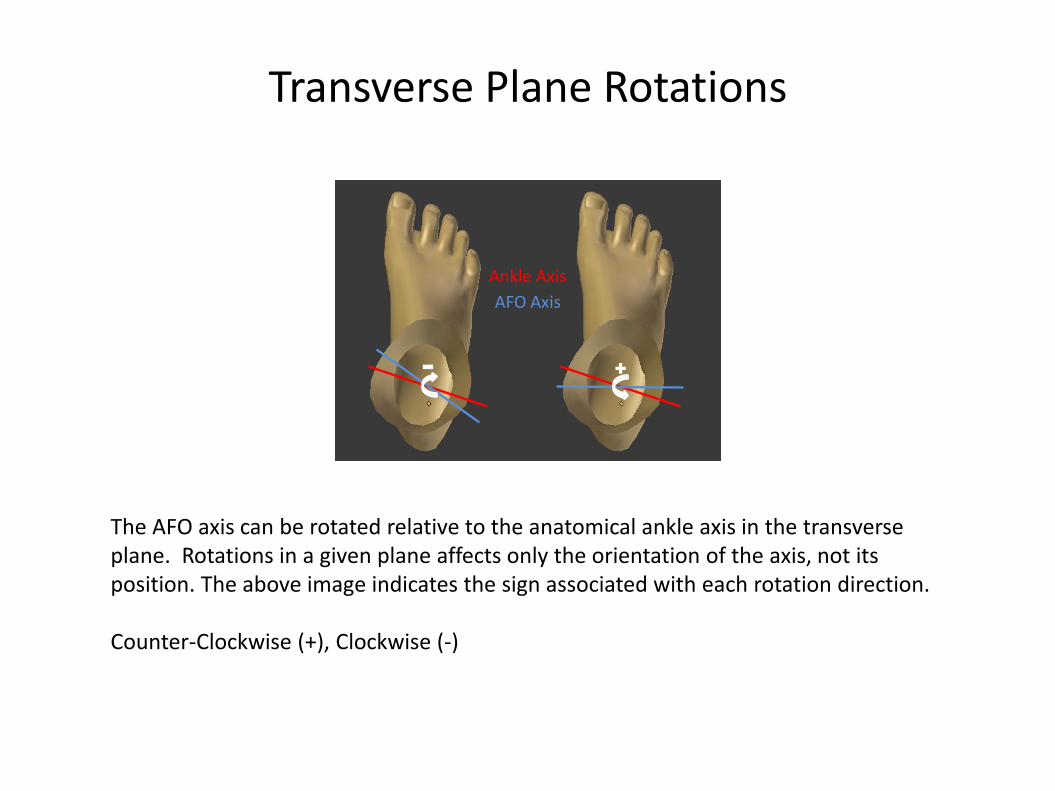
Transverse Plane Rotations

Ankle Axis

AFO Axis

The AFO axis can be rotated relative to the anatomical ankle axis in the transverse plane. Rotations in a given plane affects only the orientation of the axis, not its position. The above image indicates the sign associated with each rotation direction. Counter-Clockwise (+), Clockwise (-)

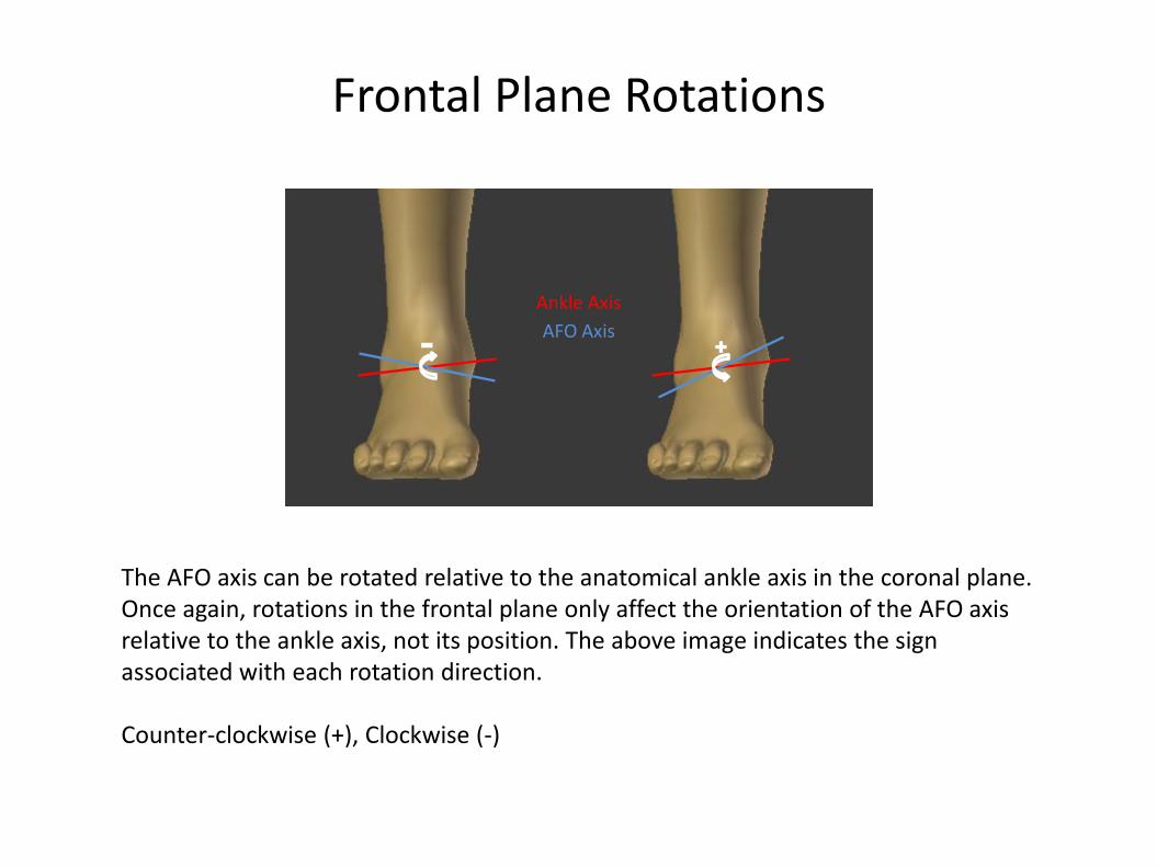
Frontal Plane Rotations

Ankle Axis

AFO Axis

The AFO axis can be rotated relative to the anatomical ankle axis in the coronal plane. Once again, rotations in the frontal plane only affect the orientation of the AFO axis relative to the ankle axis, not its position. The above image indicates the sign associated with each rotation direction. Counter-clockwise (+), Clockwise (-)

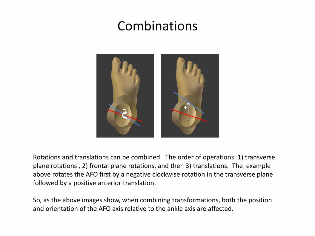
Combinations

Rotations and translations can be combined. The order of operations: 1) transverse plane rotations , 2) frontal plane rotations, and then 3) translations. The example above rotates the AFO first by a negative clockwise rotation in the transverse plane followed by a positive anterior translation. So, as the above images show, when combining transformations, both the position and orientation of the AFO axis relative to the ankle axis are affected.

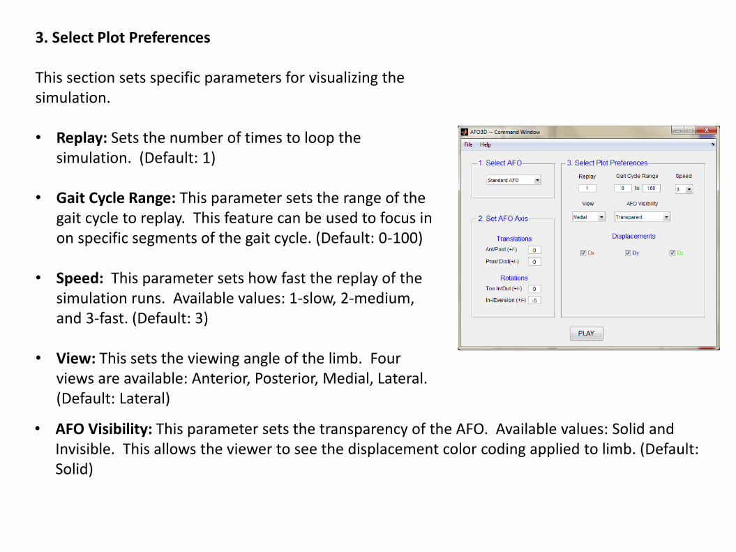
3. Select Plot Preferences This section sets specific parameters for visualizing the simulation. • Replay: Sets the number of times to loop the

simulation. (Default: 1)

• Gait Cycle Range: This parameter sets the range of the gait cycle to replay. This feature can be used to focus in on specific segments of the gait cycle. (Default: 0-100)

• Speed: This parameter sets how fast the replay of the simulation runs. Available values: 1-slow, 2-medium, and 3-fast. (Default: 3)

• View: This sets the viewing angle of the limb. Four views are available: Anterior, Posterior, Medial, Lateral. (Default: Lateral)

• AFO Visibility: This parameter sets the transparency of the AFO. Available values: Solid and Invisible. This allows the viewer to see the displacement color coding applied to limb. (Default: Solid)

• Displacements: This parameter sets which components of the tracked point’s displacement relative to the shank-based coordinate system are plotted. (Default: All selected)

1) Dx: displacements along x-axis (red plotted line) 2) Dy: displacements along y-axis (blue plotted line) 3) Dz: displacements along z-axis (green plotted line) Note: The point being tracked is fixed and is set at three-quarters of the shank length. It is located along the z-axis of the shank-based coordinate system, which passes through the ankle and knee centers.

Tracked Point

X

Z

Displacement plots of tracked point

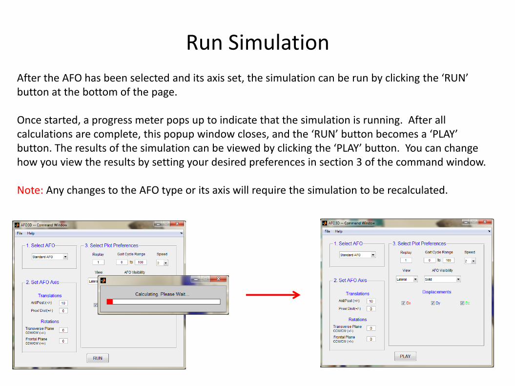
Run Simulation

After the AFO has been selected and its axis set, the simulation can be run by clicking the ‘RUN’ button at the bottom of the page. Once started, a progress meter pops up to indicate that the simulation is running. After all calculations are complete, this popup window closes, and the ‘RUN’ button becomes a ‘PLAY’ button. The results of the simulation can be viewed by clicking the ‘PLAY’ button. You can change how you view the results by setting your desired preferences in section 3 of the command window. Note: Any changes to the AFO type or its axis will require the simulation to be recalculated.

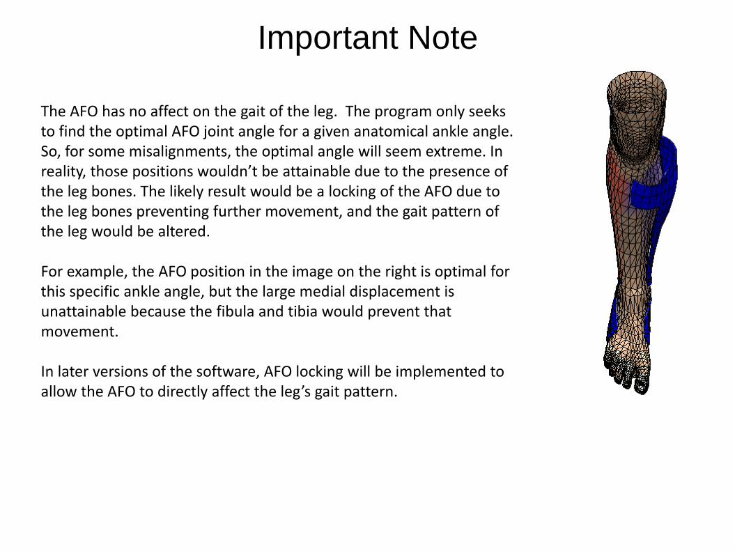
The AFO has no affect on the gait of the leg. The program only seeks to find the optimal AFO joint angle for a given anatomical ankle angle. So, for some misalignments, the optimal angle will seem extreme. In reality, those positions wouldn’t be attainable due to the presence of the leg bones. The likely result would be a locking of the AFO due to the leg bones preventing further movement, and the gait pattern of the leg would be altered. For example, the AFO position in the image on the right is optimal for this specific ankle angle, but the large medial displacement is unattainable because the fibula and tibia would prevent that movement. In later versions of the software, AFO locking will be implemented to allow the AFO to directly affect the leg’s gait pattern.

Important Note

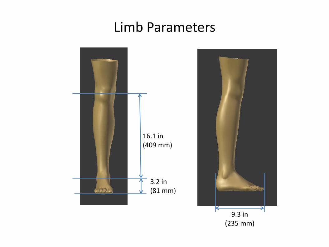
Limb Parameters

16.1 in (409 mm)

3.2 in (81 mm)

9.3 in (235 mm)