afghanistan transportation geohazard risk management … · user manual for the afghanistan...
TRANSCRIPT

JUNE
29,
201
7
U S E R M A N U A L
H T T P : / / S P A T I A L . M T R I . O R G / W B D S S
Afghanistan Transportation Geohazard Risk
Management Decision Support System

User Manual for theAfghanistan Transportation Geohazard Risk Management Decision Support SystemJune 29, 2017
H T T P : / / S P A T I A L . M T R I . O R G / W B D S S
Table of Contents1. Executive Summary …………………………………………………………………………………………………………………………………………………………………………………………………………………………………… 6
1.a. DSS Overview ……………………………………………………………………………………………………………………………………………………………………………………………………………………………………………… 7
2. User’s Manual ……………………………………………………………………………………………………………………………………………………………………………………………………………………………………………… 11
2. a. Landslide Analysis ……………………………………………………………………………………………………………………………………………………………………………………………………………………………… 11
2. b. Avalanche Analysis …………………………………………………………………………………………………………………………………………………………………………………………………………………………… 12
3. Web DSS Interface ………………………………………………………………………………………………………………………………………………………………………………………………………………………………… 13
3. a. Overview Window User Interface ……………………………………………………………………………………………………………………………………………………………………………………… 13
3. a. i. Displaying Hazard and Mitigation Analyses ………………………………………………………………………………………………………………………………………………………… 14
3. a. ii. Critical Location Assessment …………………………………………………………………………………………………………………………………………………………………………………………… 14
3. a. iii. Map Options ……………………………………………………………………………………………………………………………………………………………………………………………………………………………………… 15
3. b. Analysis Window User Interface ………………………………………………………………………………………………………………………………………………………………………………………… 15
3. b. i. Accessing the Analysis Window ……………………………………………………………………………………………………………………………………………………………………………………… 16
3. b. ii. Using the Analysis Window ………………………………………………………………………………………………………………………………………………………………………………………………… 16
3. b. iii. Interpreting the Analysis Window Plots ………………………………………………………………………………………………………………………………………………………………… 17
3. c. WMS and GIS Integration …………………………………………………………………………………………………………………………………………………………………………………………………………… 18
4. Tutorials ……………………………………………………………………………………………………………………………………………………………………………………………………………………………………………………………… 19
4. a. Interpretation of the factor of safety ……………………………………………………………………………………………………………………………………………………………………………… 19
4. b. Determine an optimal mitigation strategy ………………………………………………………………………………………………………………………………………………………………… 19
4. c. Integrating model results with GeoNode …………………………………………………………………………………………………………………………………………………………………… 23
5. Troubleshooting ………………………………………………………………………………………………………………………………………………………………………………………………………………………………………… 25
6. Appendix. Landslide hazard modeling: theory and implementation. …………………………………………………………………………………………………… 26
6.a. Models and theoretical background. ……………………………………………………………………………………………………………………………………………………………………………… 26
6.b. Model inputs and data. …………………………………………………………………………………………………………………………………………………………………………………………………………………… 28
7. References ……………………………………………………………………………………………………………………………………………………………………………………………………………………………………………………… 30

Table of FiguresFigure 1. DSS region of interest in Afghanistan …………………………… 6
Figure 2. DSS showing corridor level
earthquake-induced landslide risk. ………………………………………………………… 7
Figure 3. Comparisons of hazard maps with the application
of three mitigation strategies. ……………………………………………………………………… 8
Figure 4. Hazard zone calculated for the Profile-3 critical
location………………………………………………………………………………………………………………………………… 9
Figure 5. Hazard zone summary calculations ……………………………… 9
Figure 6. Avalanche hazard assessment ………………………………………… 10
Figure 7. The corridor-wide Hazard Analysis dashboard
menu …………………………………………………………………………………………………………………………………… 11
Figure 8. The 100-year return earthquake-induced shallow
landslide hazard West of Doshi ……………………………………………………………… 11
Figure 9. Comparison of a region without (left) and with
mitigation (right). ……………………………………………………………………………………………………… 12
Figure 10. McClung and Schaerer’s 1981 classification
system for avalanche size. …………………………………………………………………………… 12
Figure 11. Anatomy of the DSS overview window. ………………… 13
Figure 12. Hazard zone created on the fly for a user-
defined point along the corridor. …………………………………………………………… 14
Figure 13. Statistics calculated for a hazard zone for 10-
year earthquake-induced landslides. ………………………………………………… 15
Figure 14. Left: anatomy of the DSS analysis window. Right:
a fully populated analysis window. ……………………………………………………… 16
Figure 15. Hazard layer with a mitigation are identified
using a drawn polygon overlay. ……………………………………………………………… 17
Figure 16. Mitigation layer with a mitigation area identified
using a drawn polygon overlay. ……………………………………………………………… 17
Figure 17. Pixel statistics for unmitigated hazard and
mitigated hazard. …………………………………………………………………………………………………… 18
Figure 18. A custom critical location added to the overview
window. …………………………………………………………………………………………………………………………… 19
Figure 19. A hazard region generated by the DSS at a
custom critical location. ……………………………………………………………………………………20
Figure 20. An unmitigated hazard layer shown with a
custom critical location and hazard region generated by
the DSS in the overview window. ……………………………………………………………20
Figure 21. Pixel statistics for the hazard region identified at
a custom critical location. ……………………………………………………………………………… 21
Figure 22. Figures generated by the analysis window. ……… 22
Figure 23. Geonotelanding page …………………………………………………………… 23
Figure 24. Geonote Map for Schools ………………………………………………… 24
Figure 25. Illustration of source and propagation (runout)
of landslides. ………………………………………………………………………………………………………………26
Figure 26. Illustration of the infinite slope model for
landslides. …………………………………………………………………………………………………………………… 27
Figure 27. Illustration of the three-dimensional rotational
model for landslides. ………………………………………………………………………………………… 27
C O N T A C TThis Decision Support System was developed by Michigan Technological University and the Michigan Tech Research
Institute under World Bank Project P160578. The project was led by principal investigator Dr. Robert Shuchman and Dr.
Thomas Oommen. The science team members are Dr. Rudiger Escobar Wolf, Michael Battaglia, and Samuel Aden.

6
1. Executive Summary
The Afghanistan Transportation Geohazard Risk
Management Decision Support System (DSS) was
created for stakeholders to identify geohazards along
transportation corridors in northeastern Afghanistan, and
to evaluate the effectiveness of investments in geohazard
mitigation. The DSS was developed specifically for the
Baghlan to Bamiyan (B2B) Road and the Salang Highway,
two stretches of road that are particularly susceptible to
landslides and other geohazards (see Figure 1).
F I G U R E 1 . D S S R E G I O N O F I N T E R E S T I N A F G H A N I S T A N
The DSS allows users to visualize geohazards and extreme
weather risk, including landslides and avalanches, under
a variety of potential scenarios. It also enables users to
simulate mitigation techniques to quantify how hazard
severity could be reduced if such mitigation techniques
are utilized. The DSS incorporates tools to compare and
relate the effectiveness of various mitigation procedures
for each location along the road. Relative cost estimates
for mitigation scenarios are also provided.
These functionalities enable the DSS to be integrated
into the normal transport process decision cycles in
Afghanistan, from feasibility study to detailed design,
as well as operations and maintenance. The DSS can be
accessed from the following web link:
http://spatial.mtri.org/wbdss

7
1 . A . D S S O V E R V I E WThe Salang highway, which connects Kabul to the
northern regions of Afghanistan, provides one of the two
major land transportation routes through the Hindukush
region. The highway reaches elevations of 3400 m and is
susceptible to interference and damages resulting from
geological and water related hazards. Landslides and
avalanches have killed hundreds on the highway over the
last several decades. The alternative route for overland
travel through the Hindukush is the Baghlan to Bamiyan
(B2B) road, which is located at lower altitudes and is
generally less susceptible to emergencies related to slope
instability and extreme weather. However, B2B is unpaved
and almost twice the length of the Salang pass. Travel
delays and limitations along these roadways have severe
economic implications for Northeastern Afghanistan and
Kabul’s residents in particular. The DSS was created for
the purpose of aiding transportation officials’ efforts to
plan and mitigate the effects of costly geohazards in the
context of normal transport process. Presented in this
report is an executive summary and overview of the DSS,
followed by a detailed User’s Manual.
The DSS is scalable from the transportation corridor level
down to local levels at any point on the road network.
Transportation officials can easily visualize corridor-wide
geohazard assessments to evaluate large-scale mitigation
and investment plan. For example, Figure 2 is a screenshot
from the DSS that shows an earthquake-induced hazard
for a 100 year return period. On the figure 2, green
represents low hazard, yellow represents moderate
hazard, and red represents high hazard. This particular
analysis allows users to immediately assess where there
is a need for large scale mitigation efforts. In the figure
below, roughly 100 kilometers of the ~250 kilometer
corridor is classified as “low” hazard for an earthquake
magnitude that has a 100-year return period thus requires
little or no mitigation.
F I G U R E 2 . A S C R E E N S H O T O F T H E D S S S H O W I N G E A R T H Q U A K E - I N D U C E D L A N D S L I D E R I S K A T T H E C O R R I D O R L E V E L .
Utilization of the best available landscape data coupled
with a variety of geohazard modelling techniques
enabled the production of hazard maps for multiple
geohazard scenarios likely to occur in Afghanistan.
The DSS parameters can be set for a variety of hazard
types (shallow earthquake-induced landslides, deep
earthquake-induced landslide, rainfall-induced landslides)
and return periods (10-year, 50-year, 100-year, 500-year,
& 100-year). For each hazard scenario, users can assess
the change in hazard level with the implementation of
the three mitigation strategies: slope modification, soil
strength increase through mitigation measures such as

8
shortcrete, and ground water table reduction. Figure
3 shows the DSS with the 50-year deep earthquake-
induced hazard assessment displayed, followed by the
same assessment with each of the mitigation strategies
implemented. Note that lowering groundwater or soil
strength increase have minimal effect in this area
considering the fact that the landslide is caused by
earthquake. The slope modification mitigation is the most
effective in risk reduction, but it also is the most costly
to implement. This functionality will help transportation
officials find an appropriate balance between cost and
effectiveness when allocating resources to specific
remediation efforts during the course of normal
transportation corridor feasibility studies, detailed designs,
and maintenance.
F I G U R E 3 . C O M P A R I S O N S O F H A Z A R D M A P S W I T H T H E A P P L I C A T I O N O F T H R E E M I T I G A T I O N S T R A T E G I E S .
High resolution digital elevation models (DEM) were
used to calculate the hazard and mitigation along the
corridor within the DSS. This enables users to view hazard
assessments for specific localized areas of interest
anywhere along the corridor, in addition to the corridor-
wide scale in Figure 2. In Figure 4 the polygon outlined in
blue is the area on both sides of the road that is affecting
the location represented by the blue pin marker. This
region is approximately 5 square kilometers. In this way
users are able to compute hazard zones for specific points
anywhere along the road which can be added to the map
interactively.
50-year deep seismic-induced hazard assessment (no mitigation)
50-year deep seismic-induced hazard assessment (Mitigation type: slope-modification)
50-year deep seismic-induced hazard assessment (Mitigation type: Soil strength increase)
50-year deep seismic-induced hazard assessment (Mitigation type: reducing groundwater level)

9
F I G U R E 4 . H A Z A R D Z O N E C A L C U L A T E D F O R T H E P R O F I L E - 3 C R I T I C A L L O C A T I O N
The DSS has the capacity of calculating a summary for
the hazard severities within each local hazard zones. In
the example provided in the Figure 5 below, 33% of the
region is classified with high hazard pixels while 51% is
moderate hazard and 15% is low hazard. At this location
along the road over half of the area requires mitigation.
Selection and application of the various mitigation
strategies will allow transportation officials to assess how
those strategies will reduce risk. When slope modification
is applied to the area in Figure 5, high hazard is reduced to
3% while moderate and low hazard areas have increased.
F I G U R E 5 . H A Z A R D Z O N E S U M M A R Y C A L C U L A T I O N S F O R 5 0 - Y E A R E A R T H Q U A K E I N D U C E D L A N D S L I D E W I T H N O M I T I G A T I O N ( L E F T ) A N D S L O P E M O D I F I C A T I O N ( R I G H T )
10
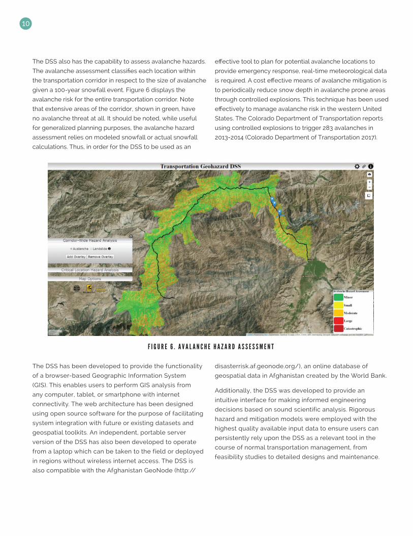
The DSS also has the capability to assess avalanche hazards.
The avalanche assessment classifies each location within
the transportation corridor in respect to the size of avalanche
given a 100-year snowfall event. Figure 6 displays the
avalanche risk for the entire transportation corridor. Note
that extensive areas of the corridor, shown in green, have
no avalanche threat at all. It should be noted, while useful
for generalized planning purposes, the avalanche hazard
assessment relies on modeled snowfall or actual snowfall
calculations. Thus, in order for the DSS to be used as an
effective tool to plan for potential avalanche locations to
provide emergency response, real-time meteorological data
is required. A cost effective means of avalanche mitigation is
to periodically reduce snow depth in avalanche prone areas
through controlled explosions. This technique has been used
effectively to manage avalanche risk in the western United
States. The Colorado Department of Transportation reports
using controlled explosions to trigger 283 avalanches in
2013-2014 (Colorado Department of Transportation 2017).
F I G U R E 6 . A V A L A N C H E H A Z A R D A S S E S S M E N T
The DSS has been developed to provide the functionality
of a browser-based Geographic Information System
(GIS). This enables users to perform GIS analysis from
any computer, tablet, or smartphone with internet
connectivity. The web architecture has been designed
using open source software for the purpose of facilitating
system integration with future or existing datasets and
geospatial toolkits. An independent, portable server
version of the DSS has also been developed to operate
from a laptop which can be taken to the field or deployed
in regions without wireless internet access. The DSS is
also compatible with the Afghanistan GeoNode (http://
disasterrisk.af.geonode.org/), an online database of
geospatial data in Afghanistan created by the World Bank.
Additionally, the DSS was developed to provide an
intuitive interface for making informed engineering
decisions based on sound scientific analysis. Rigorous
hazard and mitigation models were employed with the
highest quality available input data to ensure users can
persistently rely upon the DSS as a relevant tool in the
course of normal transportation management, from
feasibility studies to detailed designs and maintenance.
11
2. User’s Manual
B elow is a detailed description of the specific
hazard and mitigation assessments within the DSS,
as well as a step by step description of the DSS’s
functionality.
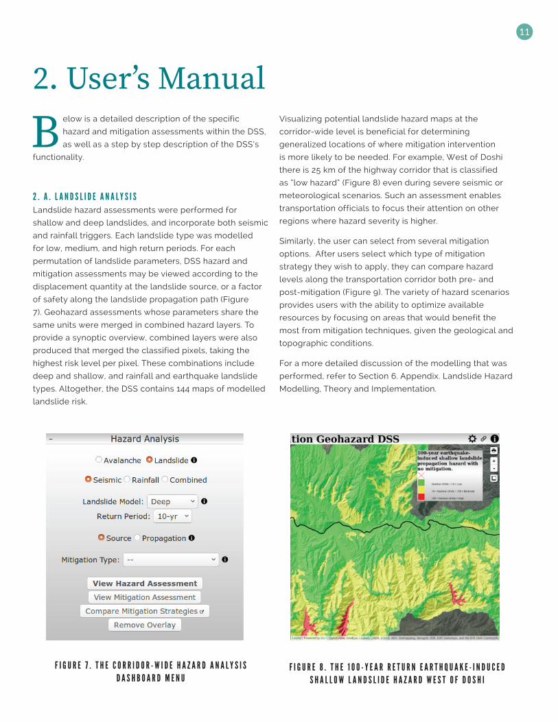
2 . A . L A N D S L I D E A N A L Y S I SLandslide hazard assessments were performed for
shallow and deep landslides, and incorporate both seismic
and rainfall triggers. Each landslide type was modelled
for low, medium, and high return periods. For each
permutation of landslide parameters, DSS hazard and
mitigation assessments may be viewed according to the
displacement quantity at the landslide source, or a factor
of safety along the landslide propagation path (Figure
7). Geohazard assessments whose parameters share the
same units were merged in combined hazard layers. To
provide a synoptic overview, combined layers were also
produced that merged the classified pixels, taking the
highest risk level per pixel. These combinations include
deep and shallow, and rainfall and earthquake landslide
types. Altogether, the DSS contains 144 maps of modelled
landslide risk.
Visualizing potential landslide hazard maps at the
corridor-wide level is beneficial for determining
generalized locations of where mitigation intervention
is more likely to be needed. For example, West of Doshi
there is 25 km of the highway corridor that is classified
as “low hazard” (Figure 8) even during severe seismic or
meteorological scenarios. Such an assessment enables
transportation officials to focus their attention on other
regions where hazard severity is higher.
Similarly, the user can select from several mitigation
options. After users select which type of mitigation
strategy they wish to apply, they can compare hazard
levels along the transportation corridor both pre- and
post-mitigation (Figure 9). The variety of hazard scenarios
provides users with the ability to optimize available
resources by focusing on areas that would benefit the
most from mitigation techniques, given the geological and
topographic conditions.
For a more detailed discussion of the modelling that was
performed, refer to Section 6. Appendix. Landslide Hazard
Modelling, Theory and Implementation.
F I G U R E 7 . T H E C O R R I D O R - W I D E H A Z A R D A N A L Y S I S D A S H B O A R D M E N U
F I G U R E 8 . T H E 1 0 0 - Y E A R R E T U R N E A R T H Q U A K E - I N D U C E D S H A L L O W L A N D S L I D E H A Z A R D W E S T O F D O S H I

12
F I G U R E 9 . C O M P A R I S O N O F A R E G I O N W I T H O U T ( L E F T ) A N D W I T H M I T I G A T I O N ( R I G H T ) .
2 . B . A V A L A N C H E A N A L Y S I SIn addition to landslide hazards, users are able to view an
analysis of avalanche hazards in the region. The avalanche
assessment, completed for a previously completed World
Bank funded effort, shows avalanche runout areas and
their associated avalanche pressure (in kPa) for a 100-year
return period snow event. The results have been classified
using a Canadian schema for classifying avalanche
severity (Figure 10, McClung and Schaerer 1981).
F I G U R E 1 0 . M C C L U N G A N D S C H A E R E R ’ S 1 9 8 1 C L A S S I F I C A T I O N S Y S T E M F O R A V A L A N C H E S I Z E .

13
3. Web DSS Interface
T he Afghanistan Transportation Geohazard DSS is
live on the web at http://spatial.mtri.org/wbdss.
This web interface provides a browser-based
environment for viewing geohazard model assessments
and comparing the effectiveness of modelled mitigation
strategies.
The model data are organized using a Geoserver instance
(http://geoserver.org/) that makes the data available as a
WMS service which may be ingested by any web-enabled
GIS (See section 3.c.).
The DSS web framework is served from an Apache server
(https://www.apache.org/) located at Michigan Tech
Research Institute in Ann Arbor, Michigan, USA. This server
hosts all website source code and handles all the web
traffic related to DSS access.
The DSS website is built around a Leaflet map viewer
(http://leafletjs.com/) with a variety of HTML widgets that
are driven by Javascript. Javascript must be enabled in
web browser settings to use the DSS.
The DSS consists of two HTML templates: an overview
window, and an analysis window. Each page’s contents
are customized to suit an analysis region. The following
sections will cover each window’s functionality in detail.
3 . A . O V E R V I E W W I N D O W U S E R I N T E R F A C E The goal of the overview window is to provide a corridor-
scale view of the risk assessment that was produced for
this decision support system. Users may browse model
results by toggling between hazard and mitigation
assessments, zooming and panning around the region,
and customizing their view of the data with various
basemaps, ancillary datasets, and user annotations. The
purpose of this design is to provide an intuitive web
environment to contextualize hazard analysis raster
layers with local geography, topology, and infrastructure.
With this visualization of the local environment, project
managers can better understand the extent of geohazards
across the entire transportation corridor region.
The interactive regions in the DSS overview window are
displayed in red in Figure 11.
• TOP BAR governs page functions.
• DASHBOARD governs map layer functions.
• LEGEND is populated when a geohazard layer is
added to the map.
• Hovering the mouse over will display tooltips
containing user assistance and item descriptions.
Clicking the in the top bar will open a copy of this
manual. When in doubt, consult the closest
F I G U R E 1 1 . A N A T O M Y O F T H E D S S O V E R V I E W W I N D O W .
TOP BAR
DASHBOARD
LEGEND

14
3. a. i. Displaying Hazard and Mitigation Analyses
DSS map and layer functionality is provided through a
dashboard interface.
The dashboard floats over the map and may be positioned
anywhere by dragging it with the mouse. It can be hidden
by clicking and restored by clicking in the top bar.
To display hazard and mitigation assessments, select
the first dashboard section and identify the desired layer
parameters. Figure 7 shows the parameters that users may
add to the map. Selecting a layer from the dashboard will
display the corridor-wide hazard or mitigation layer.
3. a. ii. Critical Location Assessment
Critical locations are named points of interest that can be
added to the map viewer for geographic reference, or to
compute the hazard areas directly threatening that point.
Users may drop custom pins anywhere on the map for
reference. In the critical locations dashboard menu, enter a
unique name and then either click the desired location
on the map, or enter known latitude and longitude
coordinates (Figure 12). To delete a critical location, click .
Once a critical location is added to the DSS, it can be
managed from the Critical Locations dashboard menu. In
the Critical Locations dashboard menu, all critical locations
are listed in a table format. The ROI column allows users
to identify a region of interest that meets DSS criteria for
geohazard threats. The DSS criteria identifies any area
whose ratio of horizontal distance to vertical elevation
exceeds a threshold value of 0.4 (Appendix 7, Figure 4).
Slopes within the identified region of interest have a high
likelihood of interfering with the critical location if they
fail. Associating these regions of interest with areas that
are classified as High- or Moderate-risk in the geohazard
modelling can provide crucial information in supporting
roadway management decisions.
Points at which detailed geohazard profiles have been
drafted are preloaded on the map. Links to reports are
contained in popups that are accessed by clicking their
icon ( ). Geohazard regions of interest may also be
requested from a critical location’s popup dialog.
F I G U R E 1 2 . H A Z A R D Z O N E C R E A T E D O N T H E F L Y F O R A U S E R - D E F I N E D P O I N T A L O N G T H E C O R R I D O R .
Once a critical location and region of interest are created,
users may request a breakdown of the geohazard risk
levels within the region of interest. If a region of interest
is requested when a hazard or mitigation layer has
already been added to the map then the statistics will be
displayed automatically. If a hazard or mitigation is added
after the region of interest is computed, then the user will
need to refresh the statistics from within the popup, by
clicking . New statistics will be appended at the bottom
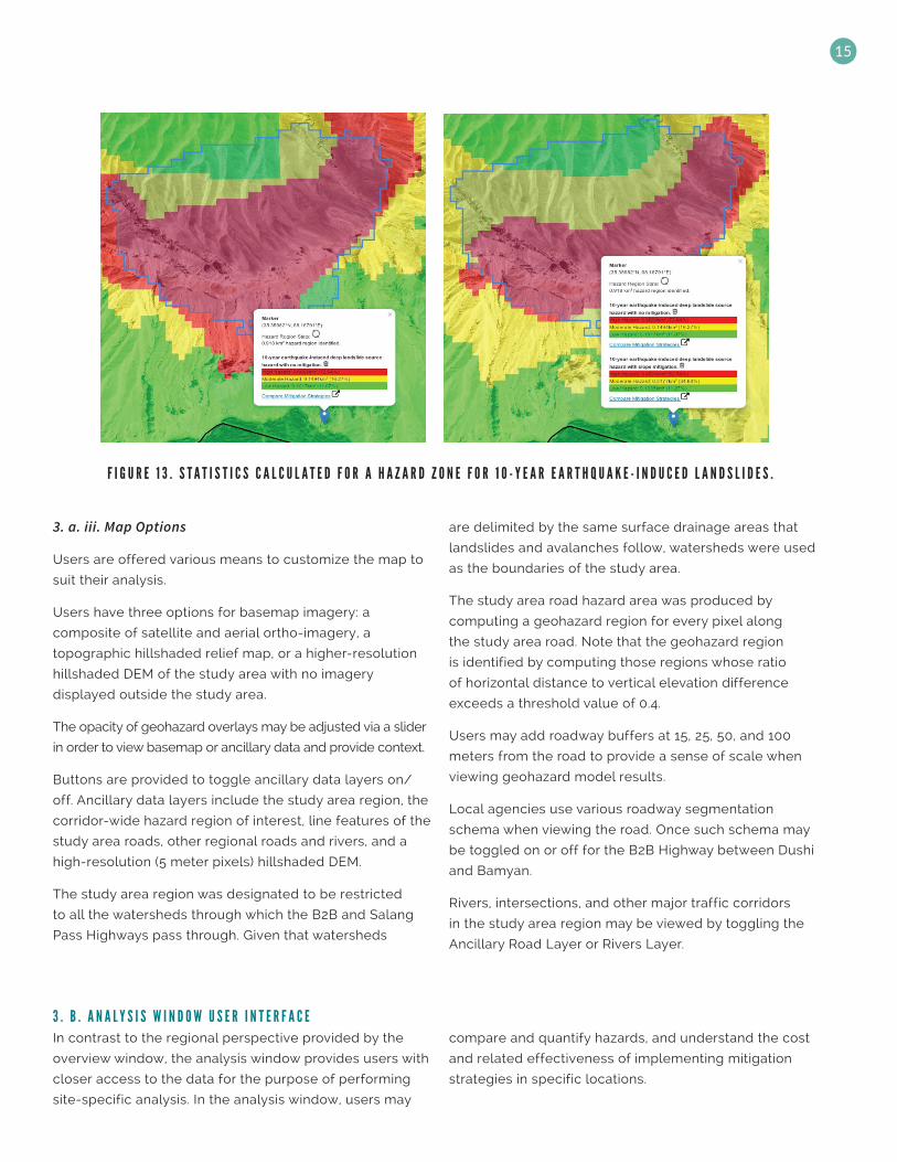
of the popup, as shown in Figure 13.
15
F I G U R E 1 3 . S T A T I S T I C S C A L C U L A T E D F O R A H A Z A R D Z O N E F O R 1 0 - Y E A R E A R T H Q U A K E - I N D U C E D L A N D S L I D E S .
3. a. iii. Map Options
Users are offered various means to customize the map to
suit their analysis.
Users have three options for basemap imagery: a
composite of satellite and aerial ortho-imagery, a
topographic hillshaded relief map, or a higher-resolution
hillshaded DEM of the study area with no imagery
displayed outside the study area.
The opacity of geohazard overlays may be adjusted via a slider
in order to view basemap or ancillary data and provide context.
Buttons are provided to toggle ancillary data layers on/
off. Ancillary data layers include the study area region, the
corridor-wide hazard region of interest, line features of the
study area roads, other regional roads and rivers, and a
high-resolution (5 meter pixels) hillshaded DEM.
The study area region was designated to be restricted
to all the watersheds through which the B2B and Salang
Pass Highways pass through. Given that watersheds
are delimited by the same surface drainage areas that
landslides and avalanches follow, watersheds were used
as the boundaries of the study area.
The study area road hazard area was produced by
computing a geohazard region for every pixel along
the study area road. Note that the geohazard region
is identified by computing those regions whose ratio
of horizontal distance to vertical elevation difference
exceeds a threshold value of 0.4.
Users may add roadway buffers at 15, 25, 50, and 100
meters from the road to provide a sense of scale when
viewing geohazard model results.
Local agencies use various roadway segmentation
schema when viewing the road. Once such schema may
be toggled on or off for the B2B Highway between Dushi
and Bamyan.
Rivers, intersections, and other major traffic corridors
in the study area region may be viewed by toggling the
Ancillary Road Layer or Rivers Layer.
3 . B . A N A L Y S I S W I N D O W U S E R I N T E R F A C EIn contrast to the regional perspective provided by the
overview window, the analysis window provides users with
closer access to the data for the purpose of performing
site-specific analysis. In the analysis window, users may
compare and quantify hazards, and understand the cost
and related effectiveness of implementing mitigation
strategies in specific locations.

16
The separate sections of the analysis window are displayed in red in Figure 14.
F I G U R E 1 4 . L E F T : A N A T O M Y O F T H E D S S A N A L Y S I S W I N D O W . R I G H T : A F U L L Y P O P U L A T E D A N A L Y S I S W I N D O W .
3. b. i. Accessing the Analysis Window
The analysis window is accessed from the overview
window in two ways:
1. When a hazard layer is added to the map,
will appear in the hazard
analysis dashboard menu. Clicking on this button will
open the analysis window in a new tab.
2. When a critical location is selected,
will appear in the critical
location’s popup as a button or hyperlinked text.
Selecting this will open the analysis window in a new
tab.
3. b. ii. Using the Analysis Window
The analysis window provides users with tools to identify
and analyze specific hazard regions and mitigation sites in
the study area region.
The analysis window’s map viewer contains all the
standard panning and zooming capabilities, and provides
the study area DEM hillshade as a basemap. The map
viewer also contains a slider, which allows users to view
hazard and mitigation assessments side-by-side and to
move the slider to change which assessment is shown in a
given area.
The spatial analysis performed by the analysis window
requires a region to be identified for analysis. This can
be the hazard region computed in the overview window,
or a drawn polygon overlay. If the analysis window was
accessed via the a critical location’s popup (option 2 in
Section 3. b. i.) and a geohazard region of interest has
been computed for that critical location, then the region
will appear in the analysis window’s map. Alternatively, the
measure tool in the analysis window’s hazard map ( )
can be used to draw a polygon for analysis. Please specify
your choice in the “Select mitigation area:” drop down
menu.
Mitigation layers may be added to the map by selecting
a mitigation strategy from the “Select mitigation type:”
drop down menu. This will also fill the “Unit Cost:” field
with a default value to be used in estimating the cost
for implementing the chosen mitigation strategy in the
designated region. These default costs are $US dollar
amounts for known Afghanistan market values from
May 2017. “Units” refer to 30 by 30 meter pixels used in
geohazard modelling. Costing may be adjusted to match
other known assessments.
Analysis can be further constrained to only consider a region
within a certain fixed distance from the roadway. These fixed
distances correspond to the DSS buffer distances of 15, 25,
50, and 100 meters. Selecting a buffer distance will display
the roadway buffer in the map viewer.
Screenshots and downloads are encouraged in the analysis
window. To download plots, right-click on the image and
select the desired function to print. URLs to generated plots
are not permanent, so exporting copies is the recommended
method to archive and distribute DSS materials.

17
3. b. iii. Interpreting the Analysis Window Plots
The analysis window provides tools to quantify hazard
and evaluate mitigation strategies in regions of interest.
If there are values or figures that are of interest that are
not directly provided by the DSS tools, those values and
figures may still be interpreted from what is available.
For example, the overview window provides users with the
area and proportion of each risk class within geohazard
regions computed according to an algorithm described
in Section 3. a. iii. If those area and proportion statistics
are desired for a drawn polygon overlay in the analysis
window, then those values may be calculated according
to the following procedure:
1. First draw a polygon to indicate your region of interest and note the total area (848,830 square meters = .85 square
km, see Figure 15). In this example, the following mountain top is used:
2. Choosing slope modification as a mitigation strategy will display the mitigation assessment with a polygon
indicating the designated region of interest (Figure 16):
F I G U R E 1 5 . H A Z A R D L A Y E R W I T H A M I T I G A T I O N A R E A I D E N T I F I E D U S I N G A D R A W N P O L Y G O N O V E R L A Y .
F I G U R E 1 6 . M I T I G A T I O N L A Y E R W I T H A M I T I G A T I O N A R E A I D E N T I F I E D U S I N G A D R A W N P O L Y G O N O V E R L A Y .

18
3. Clicking GO beneath the mitigation parameters will generate the following plots:
4. By looking at the CDF curve we can interpret the proportions. For the plot (Figure 17) with no mitigation applied
on the left, 15.86% of the pixels are classified as High hazard, 21.1% (36.96-15.86 = 21.1) are Moderate hazard, and
48.18% are Low hazard. These can be multiplied by the total area to obtain values of 134,624 square meters for High
hazard, 179,103 square meters for Moderate hazard, 408,966 square meters for Low hazard. For the plot with slope
modification applied on the right, 2.19% of the pixels are classified as High hazard, 21.31% are Moderate hazard, and
76.9% are Low hazard. The total area for each hazard class in the mitigation assessment is therefore 18,589 square
meters for High hazard, 180,885 square meters for Moderate hazard, and 652,750 square meters for Low hazard.
5. The unit cost can be applied to the total area to obtain a cost estimate for achieving this geohazard risk reduction.
In this example, using the default slope modification cost value (US$7010) across the entire mitigation area of
848,830 square meters (.85 square kilometers), would yield an estimate of US$6,611,442.
3 . C . W M S A N D G I S I N T E G R A T I O NGeohazard assessment data layers are stored using
Geoserver software (http://geoserver.org), and may be
viewed in web GIS environments.
To view DSS data layers in any internet-connected GIS,
use the following as the WMS Server URL:
http://geoserver2.mtri.org/geoserver/WBDSS/
wms?request=GetCapabilities
All model results and ancillary data products are
persistently available via the above link as a WMS service.
F I G U R E 1 7 . P I X E L S T A T I S T I C S F O R U N M I T I G A T E D H A Z A R D ( L E F T , F I G U R E 1 5 ) A N D M I T I G A T E D H A Z A R D ( R I G H T , F I G U R E 1 6 ) .
19
4. Tutorials4 . A . I N T E R P R E T A T I O N O F T H E F A C T O R O F S A F E T YThe factor of safety (Fs) is the ratio of resisting to
destabilizing forces acting on a slope, such that when the
Fs value is larger than 1 the slope is stable, and when the
Fs value is less than 1 the slope is unstable (Chowdhury
et al. 2010). Given the uncertainty in modeling results, it
is commonly assumed that values of Fs above but close
to 1 are not entirely stable but rather “marginally stable”,
and could become unstable if conditions changed slightly
or the input data to the model were slightly inaccurate. It
is common practice to consider the minimum acceptable
factor of safety FS = 1 for pseudo-static seismic slope
stability analysis, whereas a slightly larger minimum factor
of safety (e. g. FS = 1.25) is used for other conditions, e.
g. shear-friction method (e. g. Association of State Dam
Safety Officials, 2017). For each modelling method applied
the factor of safety can be interpreted in slightly different
way, depending on the model reliability and the level of
uncertainty in the model inputs.
For the precipitation triggered landslides, the modeled
results include the estimated factor of safety at each
location (pixel) in the area analyzed, as described in more
detailed in the appendix and the references cited in it. The Fs
values are highly sensitive to the inputs (e. g. Soil cohesion,
friction angle, water table depth, water table depth, hydraulic
conductivity, and hydraulic diffusivity) and can rapidly
change in some cases, even if the input parameters only
change slightly. For this reason we recommend using a
minimum Fs value of 1.25 when considering what areas
may be unstable, to account for the multiple, and probably
interacting uncertainties in the modeling process.
The seismic triggered instability modeling is based on
standard limit equilibrium (e. g. extension of Bishop’s
method to three-dimensional cases) and Newmark
displacement analyses (Chowdhury et al. 2010). The limit
equilibrium analysis performed here for deep rotational
slope failure considers worst case scenario input
parameters (e. g. relatively low strength parameters) and
we consider it’s not necessary to be additionally cautious
about the obtained Fs values. A similar rationale applies to
the Newmark displacement analysis for shallow landslides
triggered by earthquakes, particularly since we took a
relatively conservative approach when converting the
Newmark displacement values to equivalent Fs values;
displacement values of only 5 and 15 cm where chosen
for the limits between stable and marginally stable, and
marginally stable and unstable classes, respectively,
which in some cases (see Jibson et al., 2000) could
correspond to only ~ 10 % and ~ 30 % probability of failure.
For these reasons, we recommend using a minimum Fs
value of 1 when considering what areas may be unstable.
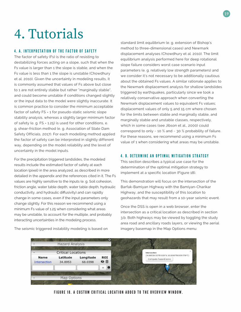
4 . B . D E T E R M I N E A N O P T I M A L M I T I G A T I O N S T R A T E G YThis section describes a typical use case for the
determination of the optimal mitigation strategy to
implement at a specific location (Figure 18).
This demonstration will focus on the intersection of the
Barfak-Bamiyan Highway with the Bamiyan-Charikar
Highway, and the susceptibility of this location to
geohazards that may result from a 10-year seismic event.
Once the DSS is open in a web browser, enter the
intersection as a critical location as described in section
3.b. Both highways may be viewed by toggling the study
area road and ancillary roads layers, or viewing the aerial
imagery basemap in the Map Options menu:
F I G U R E 1 8 . A C U S T O M C R I T I C A L L O C A T I O N A D D E D T O T H E O V E R V I E W W I N D O W .
20
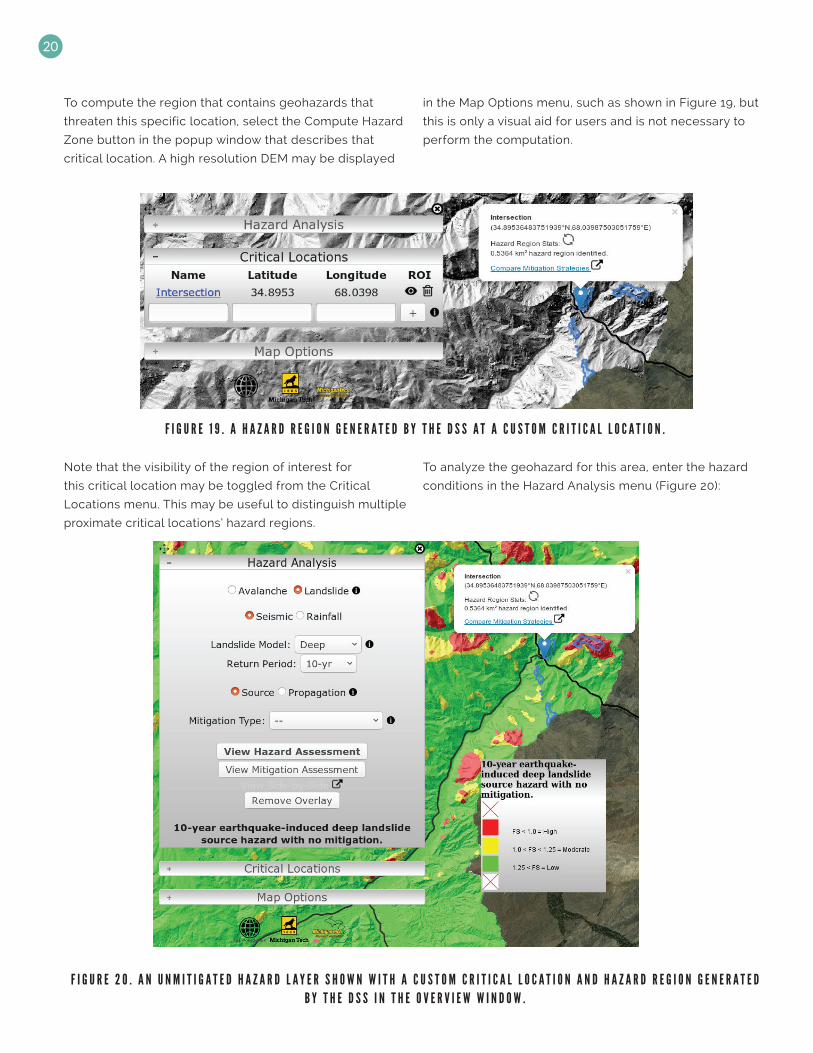
To compute the region that contains geohazards that
threaten this specific location, select the Compute Hazard
Zone button in the popup window that describes that
critical location. A high resolution DEM may be displayed
in the Map Options menu, such as shown in Figure 19, but
this is only a visual aid for users and is not necessary to
perform the computation.
F I G U R E 1 9 . A H A Z A R D R E G I O N G E N E R A T E D B Y T H E D S S A T A C U S T O M C R I T I C A L L O C A T I O N .
Note that the visibility of the region of interest for
this critical location may be toggled from the Critical
Locations menu. This may be useful to distinguish multiple
proximate critical locations’ hazard regions.
To analyze the geohazard for this area, enter the hazard
conditions in the Hazard Analysis menu (Figure 20):
F I G U R E 2 0 . A N U N M I T I G A T E D H A Z A R D L A Y E R S H O W N W I T H A C U S T O M C R I T I C A L L O C A T I O N A N D H A Z A R D R E G I O N G E N E R A T E D B Y T H E D S S I N T H E O V E R V I E W W I N D O W .

21
To view a summary of the hazard levels in the region
identified as posing a threat to the highway intersection,
refresh the hazard region statistics in the popup window
(Figure 21):
F I G U R E 2 1 . P I X E L S T A T I S T I C S F O R T H E H A Z A R D R E G I O N I D E N T I F I E D A T A C U S T O M C R I T I C A L L O C A T I O N . W H E N A N E W H A Z A R D L A Y E R I S S E L E C T E D , N E W P I X E L S T A T I S T I C S A R E A P P E N D E D T O T H E P O P U P ( L E F T ) .
Note that adding a new hazard or mitigation assessment
layer will allow users to refresh the summary statistics
in the popup window. New summary statistics will be
appended to the popup window, so that users can make
preliminary comparisons between hazard conditions and
mitigation assessments. In this example, the difference
between 10-year and 100-year seismic events is minor.
To determine the optimal mitigation strategy to reduce
the geohazard risk at this location, click the Compare
Mitigation Strategies link below the summary statistics for
the particular geohazard assessment to be mitigated. This
will open a new window.
In this new window, the hazard assessment is displayed
on the left, and mitigation assessments will be displayed
on the right. A plot on the left is generated that displays
a histogram and cumulative density distribution of the
actual numeric geohazard magnitudes in the region
identified by the DSS (Figure 22). This demonstrates the
severity of risk within the region more precisely than the
low/moderate/high classification provided in the previous
corridor-wide view.
On the right, there is a drop-down menu that allows
users to select between mitigation strategies whose
effectiveness has been modeled using the specified
conditions. Once the user selects a mitigation assessment,
the data is displayed on the right side of the map viewer
at the top of the page under a slider that users may slide
back and forth, comparing the hazard and mitigation
assessments. The histogram and cumulative density
distribution for the mitigation layer will also be plotted for
the mitigation layer’s data, below the map viewer, and to
the right of the hazard data plot.

22
The figure 22 shows the material generated when slope modification is applied to these hazard conditions.
F I G U R E 2 2 . F I G U R E S G E N E R A T E D B Y T H E A N A L Y S I S W I N D O W . T O P M A P S H O W S U N M I T I G A T E D H A Z A R D A N A L Y S I S , B O T T O M M A P S H O W S S L O P E M I T I G A T E D H A Z A R D A N A L Y S I S . L E F T P L O T S H O W S U N M I T I G A T E D P I X E L S T A T S , R I G H T P L O T S H O W S P I X E L
S T A T S O N C E S L O P E M O D I F I C A T I O N H A S B E E N I M P L E M E N T E D .

23
4 . C . I N T E G R A T I N G M O D E L R E S U L T S W I T H G E O N O D EThe World Bank Group has collected several national
datasets for Afghanistan that have been made available
at http://disasterrisk.af.geonode.org/. As of June 2017,
GeoNode contains 93 unique geospatial datasets that
comprise 11 maps that are used in regional analyses of
various disaster risks.
F I G U R E 2 3 . G E O N O D E L A N D I N G P A G E .
Model results that are used in the DSS may also be
viewed in GeoNode maps. For example, figure 23 displays
the GeoNode map for “Schools, landslides, and floods,”
which consists of geohazard assessments of flood hazard
and landslide susceptibility, overlaid with national data
representing the locations and sizes of universities, high
schools, secondary schools, and primary schools.

24
F I G U R E 2 4 . G E O N O D E M A P F O R S C H O O L S , L A N D S L I D E S , A N D F L O O D S , D I S P L A Y I N G U N I V E R S I T I E S A N D B O T H R I S K A S S E S S M E N T S .
To add DSS modelling products to GeoNode maps, we will
be using the WMS service described in section 3. c.
Clicking in the top left of the window allows users to
“Add layers”. In the drop-down menu that appears, select
“Add a new server…”. Ensure the server “Type” is “Web Map
Service (WMS)”, and enter the DSS model results’ WMS
URL:
http://geoserver2.mtri.org/geoserver/WBDSS/
wms?request=GetCapabilities
Once the WMS URL is entered, clicking will show a list
of all the layers available to be used as hazard layers,
mitigation layers, or ancillary data layers in the DSS.
25
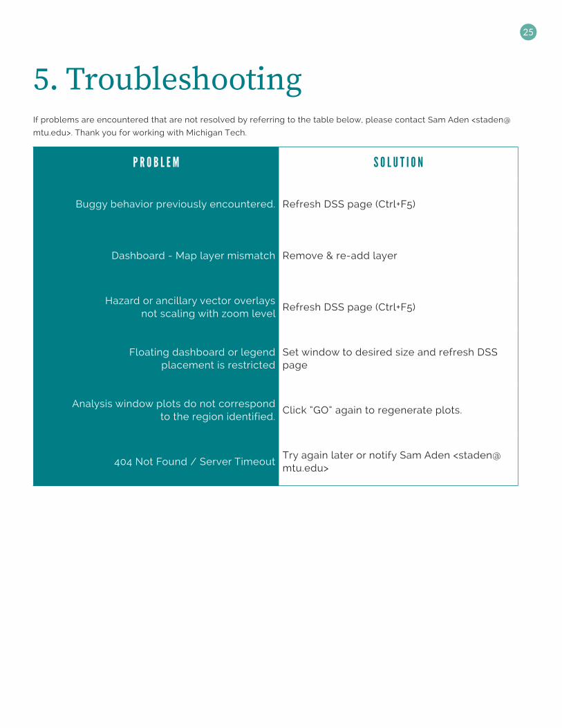
5. TroubleshootingIf problems are encountered that are not resolved by referring to the table below, please contact Sam Aden <staden@
mtu.edu>. Thank you for working with Michigan Tech.
P R O B L E M S O L U T I O N
Buggy behavior previously encountered. Refresh DSS page (Ctrl+F5)
Dashboard - Map layer mismatch Remove & re-add layer
Hazard or ancillary vector overlays not scaling with zoom level
Refresh DSS page (Ctrl+F5)
Floating dashboard or legend placement is restricted
Set window to desired size and refresh DSS page
Analysis window plots do not correspond to the region identified.
Click “GO” again to regenerate plots.
404 Not Found / Server TimeoutTry again later or notify Sam Aden <[email protected]>

26
6. Appendix. Landslide hazard modeling: theory and implementation.6 . A . M O D E L S A N D T H E O R E T I C A L B A C K G R O U N D .Landslide hazard was assessed for a variety of potential
future hazard conditions. Although landslides can happen
independently of the occurrence of any obvious triggers,
most landslides are triggered by external environmental
factors. Our initial assessment of the conditions for the
B2B and Salang Pass roads suggested that two main
processes may be the main landslides triggers in the
area: water infiltration in the soil due to precipitation
(as both rainfall and, snow and ice water melting), and
ground shaking due to earthquakes. A variety of landslide
mechanisms and types have been established (Hungr et
al. 2014 and references therein), but here we consider
only two main types of landslides that we estimate cover
most cases that we would expect to encounter in the
terrain being analyzed: shallow translation landslides, and
deep rotational landslides. Assessing the landslide hazard
involves determining the areas that could potentially
become unstable, and if such instabilities occurred,
how far would the sliding material move. Therefore,
two processes associated with the hazard need to be
assessed, the sources process and the propagation
process (see Figure 25).
F I G U R E 2 5 . I L L U S T R A T I O N O F S O U R C E A N D P R O P A G A T I O N ( R U N O U T ) O F L A N D S L I D E S . M O D I F I E D F R O M H T T P : / / P U B S . U S G S . G O V / F S / 2 0 0 4 / 3 0 7 2 / P D F / F S 2 0 0 4 - 3 0 7 2 . P D F

27
The first step in assessing the landslides hazard was to
model the conditions that would lead to slope instability
and landslide initiation. In shallow landslides the unstable
portion of the slope is confined to a zone close to surface
and it is usually assumed that its geometry is rather
simple (the failure surface extends parallel to the surface).
Our models for this type of instability are based on the
“infinite slope” (see figure 26) concept (Chowdhury et al.
2010), modified for rainfall induced landslides (Baum et
al, 2002) and earthquake triggered landslides (Jibson,
2007). For shallow landslides triggered by precipitation
the TRIGRS model was used (Baum et al, 2002), shallow
landslides triggered by earthquakes were modeled with
the Newmark displacement method (Jibson, 2007), and
deep landslides triggered by earthquakes were modeled
with the Scoops3D model (Reid et al. 2015). The triggering
of deep rotational landsides by water infiltration is less
common, but is also less well understood, in this work we
did not directly account for such cases in our modeling.
The inclusion of the other cases should in any case be
extensive enough that areas that could potentially fail as
deep landslides triggered by water infiltration are for the
most cases already covered by the other cases.
F I G U R E 2 6 . I L L U S T R A T I O N O F T H E I N F I N I T E S L O P E M O D E L F O R L A N D S L I D E S . M O D I F I E D F R O M U S G S H T T P S : / / P U B S . U S G S .G O V / O F / 2 0 0 8 / 1 1 5 9 / D O W N L O A D S / P D F / O F 0 8 - 1 1 5 9 . P D F
In deep landslides the unstable portion of the slope can extend further down and have a much more complex
geometry. Our models are based on the three dimensional rotational landslide model (Reid et al. 2015) (see Figure 27).
F I G U R E 2 7 . I L L U S T R A T I O N O F T H E T H R E E - D I M E N S I O N A L R O T A T I O N A L M O D E L F O R L A N D S L I D E S . M O D I F I E D F R O M U S G S H T T P S : / / P U B S . U S G S . G O V / T M / 1 4 / A 0 1 / P D F / T M 1 4 - A 1 . P D F

28
After the sources area for a landslide has become
unstable, the landslide mass moves downslope,
potentially reaching areas where population and
infrastructure may be exposed. Therefore, additionally
to the generation of the landslide by slope instability
processes it is also necessary to assess the landslide
mass propagation process, to evaluate what areas may
be exposed to the hazard. To model the propagation the
height to length concept, also know as energy line (or
cone, in three dimensions) was used (Hunter and Fell,
2003; Finlay et al. 1999).
Models assess slope stability through the infinite slope
model for shallow translational landslides, and by the Bishop
circular failure models for deep rotational landslides. Water
infiltration (rainfall and snowmelt) triggered landslides is
modeled in detail using the TRIGRS software published
by Baum et al. (2009) from the Unites States Geological
Survey (USGS), which combines the infinite slope model
with saturated (suction reduction) and non-saturated (pore
pressure increase) reduction of soil strength in response to
the water infiltration. This model predicts the factor of safety
of points on the landscape subject to a given rainfall intensity
and duration (Baum et al, 2002).
The seismic ground motion triggering effect was
modeled through pseudo-static analysis incorporating
Newmark displacement analysis for critical peak ground
acceleration (PGA) levels. For shallow slopes we use
the infinite slope model, coupled with a Newmark
seismic displacement model (Jibson, 2007), which
considers the stability of the slope in terms of the slope
deformation. The output of the model is not an Fs value,
but a deformation, to make this deformation compatible
with other hazard assessment outputs we converted
the displacement values to equivalent Fs. For the deep
seismic triggered landslide modeling we used the
SCOOPS3D computer program published by the Unites
States Geological Survey (USGS) (Reid et al. 2015), which
outputs results as Fs value maps.
Selection of infiltration (from rainfall and snowmelt)
events scenarios and probabilities was guided by the
prior analysis on flooding hazard, which will also allow for
consistency of our work with the results from previous
work components. The database on rainfall events
compiled for the GeoNode portal was used for this
analysis for five return periods: 10, 50, 100, 500, and 1000
years. Ground shaking intensities (PGA) from the same
source and for the same return periods was also used.
The potential propagation of the landslides was assessed
considering the height to runout ratio approach (Hunter
and Fell, 2003; Finlay et al. 1999). This approach considers
how far a landslide mass will reach from its source location,
by taking into account how much elevation it loses along
its trajectory. This roughly corresponds with the physical
concepts of driving energy, i.e. the potential gravitational
energy that allows the landslide to move in the first place
(represented by the elevation drop), and resistive frictional
energy, i.e. the energy dissipation that the landslide mass
experiences as it moves along its trajectory (represented by
the distance traveled). The ratio between the height drop
(H) and runout distance (L), H/L then becomes a measure
of the landslide’s mobility that can be applied to different
topographic settings. Although limited in many aspects,
this mobility measure is relatively easy to evaluate, as it
only depends on the topography, and it has been found
that it correlates with the landslide volume. For our analysis
purpose we used a constant value for the H/L ratio of 0.4,
representing typical landslides in the range of 104 – 105 m3,
a range of values expected to be an average for landslides
in the analyzed area.
6 . B . M O D E L I N P U T S A N D D A T A .The input data for the models used in our analysis include
data on topography, soil and rock properties, and potential
triggering events (rainfall and earthquakes). Topography
was represented through digital elevation models (DEMs)
from which slope inclination values used in the shallow
landslide models were derived. Analyses were performed
on DEMs of different resolutions, mainly a 5 m resolution
local DEM for Afghanistan, and the 30 m resolution SRTM
DEM (USGS, 2017). The final aggregated results are
presented in the 30 m resolution to precisely represent
the limiting resolution in our analysis.
Physical processes based models for slope stability
analysis require the strength properties of the slope
materials as an input into the model. Commonly the
materials’ strength is characterized through the internal
friction angle (φ) and the cohesion (c). These values are
usually obtained from laboratory tests on samples of slope
material, but can also be estimated from proxies in the field.
In this case, soil and rock properties (strength parameters,
densities and weights, grainsize distributions) were based
on a sample of geotechnical testing data provided by the
Afghan counterparts for a limited number of sampling sites
along the B2B road. Other material physical parameters

29
used by the models (e. g. rock, soil and regolith unit
weights) are less critical to know with precision and were
estimated from the same geotechnical reports.
Knowing the hydrologic properties (such as diffusivity,
saturated conductivity, etc.) of the slope materials is
also necessary for applying the models we used. Such
properties were derived based on grainsize distribution
and its relationship to geotechnical properties. Estimates of
the water table level for some wells in the area have been
reported by the USGS (Mack et al. 2014). A global water
table model was also used (Fan and Miguez-Macho, 2013)
and refined to a higher resolution to match the resolution
of the other datasets, using the height above drainage
concept (Nobre et al, 2011). Similarly, a global dataset on
soil and regolith (Pelletier et al., 2016) depth was used and
refined using a correlation with terrain slope.
The same models were used with modified input
parameters to simulate the effect of different mitigation
strategies. Slope terrain modification was modeled
by representing terrain with lower slope values in all
models, but only for the highest slope values. The
lower slope terrain model was used for input in all
modelling programs, with all other input parameters held
constant, to evaluate the effect on the model outputs,
and take those differences as the terrain performance
improvement under the landslide triggering conditions. In
practice a similar effect could be attained through cut-
and-fill techniques of the potentially unstable slopes,
complemented by some minor retaining structures and
erosion control measures. A similar approach was used to
model the effect of increasing the soil strength, changing
the value of cohesion in the inputs for the models. The
increase in cohesion could be equivalent to the effect
that some simple slope stabilization techniques could
have (e. g. minor retaining structures and erosion control
measures). In the case of drainage improvement, the
effect was modeled by accounting for a deepening of the
water table, as such could be the effect of improving the
drainage on the slopes.
30
7. ReferencesAssociation of State Dam Safety Officials, “State Seismic
Criteria. From ASDSO Survey on State-of-Practice
References and Issues, November 1999. Association of
State Dam Safety Officials” 2017. Visited online (June
2017): http://www.damsafety.org/media/Documents/
Surveys/1999SeismicCriteria.pdf
Baum, Rex L., William Z. Savage, and Jonathan W.
Godt. “TRIGRS—a Fortran program for transient rainfall
infiltration and grid-based regional slope-stability
analysis.” US geological survey open-file report 424 (2002):
38.
Chowdhury, Robin, Phil Flentje, and Gautam Bhattacharya.
Geotechnical slope analysis. Vol. 737. Balkema: Crc Press,
2010.
Colorado Department of Transportation. 2017. “Avalanche
Control”. https://www.codot.gov/travel/winter-driving/
AvControl.html. Accessed April 22, 2017.
Fan, Ying, H. Li, and Gonzalo Miguez-Macho. “Global
patterns of groundwater table depth.” Science 339.6122
(2013): 940-943.
Finlay, P. J., G. R. Mostyn, and R. Fell. “Landslide risk
assessment: prediction of travel distance.” Canadian
Geotechnical Journal 36.3 (1999): 556-562.
Hungr, Oldrich, Serge Leroueil, and Luciano Picarelli.
“The Varnes classification of landslide types, an update.”
Landslides 11.2 (2014): 167-194.
Hunter, Gavan, and Robin Fell. “Travel distance angle for”
rapid” landslides in constructed and natural soil slopes.”
Canadian Geotechnical Journal 40.6 (2003): 1123-1141.
Jibson, Randall W. “Regression models for estimating
coseismic landslide displacement.” Engineering Geology
91.2 (2007): 209-218.
Nobre, A. D., et al. “Height Above the Nearest Drainage–a
hydrologically relevant new terrain model.” Journal of
Hydrology 404.1 (2011): 13-29.
McClung, David M., and Peter A. Schaerer. 1980.”Snow
avalanche size classification.” Proceedings of Avalanche
Workshop. Vol. 3. No. 5.
Pelletier, Jon D., et al. “A gridded global data set of soil,
intact regolith, and sedimentary deposit thicknesses for
regional and global land surface modeling.” Journal of
Advances in Modeling Earth Systems (2016).
Reid, Mark E., et al. “Scoops3D—Software to Analyze
Three-Dimensional Slope Stability Throughout a Digital
Landscape.” Tech. Rep. US Geological Survey Techniques
and Methods, book 14. 2015. 218.
USGS, 2017. Shuttle Radar Topography Mission (SRTM)
1 Arc-Second Global. https://lta.cr.usgs.gov/SRTM1Arc
(accessed, May 2017).

31

32
JUNE
29,
201
7
H T T P : / / S P A T I A L . M T R I . O R G / W B D S S