AEROSOL REMOTE SENSING OVER OCEAN IN GLINT CONTAMINATED REGIONS USING AATSR AND MERIS

Rene Preusker, Juergen Fischer

Freie Universität Berlin, Carl-Heinrich-Becker-Weg 6-10, 12165 Berlin, Germany

1. INTRODUCTION

The Medium Resolution Imaging Spectrometer MERIS and the Advanced Along-Track Scanning Radiometer

AATSR instruments, both onboard ESA’s Environmental Satellite ENVISAT, provide similar spatial resolution

and swath, but complementary information, encompassing different spectral domains and viewing geometries.

Recent geophysical algorithms do not take advantage of a synergetic use of the measurements of both

instruments, although the benefits in cloud and aerosol retrieval are obvious. This paper presents one example for

a synergistic use of MERIS and AATSR imagery: The retrieval of aerosol optical thickness and Angstroem

coefficient over the ocean, in particular in sun glint contaminated regions. Later we will extend the focus on the

potential of the estimation of aerosol absorption by means of its single scattering albedo.

2. MERIS AND AATSR IN SHORT

MERIS is an imaging spectrometer with 15 programmable spectral bands in the range 400nm – 1050nm. The

operational band setting positions of the 15 bands are between 412.5nm and 900nm, including one narrow

channel at 761.375nm in the O2 A-band absorption band, two bands to estimate the integrated water vapour

content, and three bands to the retrieve aerosol properties. The MERIS swath covers 1150km across track. The

original pixel size is 260m x 300m in nadir with a slight increase towards the edge of the swath. The full

resolution data (FR) are spatially integrated (4x4 pixel) to the reduced resolution (RR) pixel with a 1040m x

1200m pixel size.

AATSR is a scanning radiometer with 7 spectral channels at visible, reflected infra-red and thermal infrared

wavelengths with two ~500 km wide curved swaths, with 555 pixels across the nadir swath and 371 pixels across

the forward swath. The nominal pixel size is 1km2 at the centre of the nadir swath and 1,5 km2 at the centre of the

forward swath. This unique feature provides two views of the surface and improves the capacity for atmospheric

correction and enables observations of the ocean surface under a tilt angle of ~46.9° in forward direction. The

first 3 AATSR bands cover MERIS channels, however, the bandwidth of the AATSR channels is significantly

larger.

2. THE ALGORITHM IN SHORT

The aerosol retrieval algorithm consists of three parts. The first part is the estimation of the ocean specular

reflection at 3.7 micron, whereby an estimation of the thermally emitted part at 3.7 from the brightness

temperatures at 11 and 12 micron is used. The thermal emitted radiance is subtracted from the top of atmosphere

radiance and corrected for water vapour, resulting in the specular reflectance at 3.7 micron. The second part is

the propagation of this reflectance a) to the MERIS channel wavelength (taken into account the wavelength

dependence of the water refractive index) and b) to the corresponding MERIS observation geometry, which is

necessary to account for the different scanning methods of MERIS (line scanner) and AATSR (conical scanner).

The third part is the estimation of the aerosol optical properties (AOT at 550nm and Angstroem coefficient)

utilizing the sea surface reflection as the lower boundary condition in a physical inversion.

2.1. Solar portion and specular reflection at 3.7 m

The top of atmosphere radiance at AATSR channel at 3.7 m top of atmosphere radiance consists of reflected

and scattered solar radiation as well as emitted radiation from the atmosphere and the surface. For cloud free

conditions the amount of molecular scattering is negligible ( < 0.00005), the amount of aerosol scattering is very

small and, compared to the amount of reflected and emitted radiation, negligible as well. (Under special

conditions, in particular for high aerosol loadings due to desert outbreaks or for undetected clouds, this may be

different, but it is not considered here). Therefore we can assume the following equation:

LTOA = Lsurf,E + Latm,E + Lsurf,S

With LTOA,E = Lsurf,E + Latm,E , the top of atmosphere radiance without any solar radiation, as it is observed e.g.

during night, the sum can be further simplified and the equation can be rearranged to:

Lsurf,S = LTOA - LTOA,E .

The estimation of LTOA,E is done by a linear regression of the measured brightness temperature at 11 m and

12 m (BT11 and BT12) to the brightness temperature at 3.7 m (BT3.7):

BT3.7 = a + b • BT11 + c • (BT11 - BT12)

The regression coefficients are: a = 4.91348 b = 0.978489 c = 1.37919. The coefficients have been found by

analyzing cloud free sea surface night scenes. The intensive quantity BT3.7 is converted into the extensive

radiance LTOA,E. by a simple linear interpolation in an appropriate look up table LTOA,E = LUT [BT3.7]. Finally

Lsurf,S is corrected for water vapor transmission T3.7 and solar irradiation to obtain the bottom of atmosphere

reflectance at γ3.7.=Lsurf,S / (E0 T3.7)

2.2. Geometrical and spectral conversion of the glint at 3.7 m

The glint at MERIS wavelengths and MERIS viewing geometry is not equal to γ3.7 because i) the refractive

index of water is different at the visible and 3.7 micron and more important and more difficult to solve ii) the

azimuth difference of the AATSR observation is different to the azimuth difference of the MERIS. The main

quantity for this geometrical conversion is the effective wind-speed ws. It is assumed that there exists a unique

relationship CM between the glint γ at a specific wavelength λ, the observation geometry (ϑsun , ϑview , diff), the

refractive index of sea water at that wavelength n and the wind-speed ws.

= CM (ϑsun , ϑview , diff ,n, ws)

But studies have shown, that this relation does not exist, at least not precisely. In particular the wind direction,

existing (cross) swell and the history of the waves modulate the relationship and lead to different

parameterizations of sea surface roughness. The task of the wind-speed ws is solely to act as a consistent

parameter for the sea surface glint. Since ws is the only unknown in the upper simplified relationship, there could

be an unique inverse solution:

ws = CM-1 (ϑsun , ϑview , diff ,n, γ)

Under the assumption that the unique inverse CM-1 exists, the geometrical conversion is straight forward and

consists of the following two steps:

i) Calculation of the effective wind-speed

ws = CM-1 (ϑsun , ϑview , AATSR ,n3.7, γ3.7)

ii) Calculation of the glints γMERIS

γMERIS = CM (ϑsun , ϑview , MERIS ,nMERIS, ws)

The forward operator CM is implemented and approximated by a look up table. The inverse operator CM-1

could not be approximated by an analytic function, because under some conditions or geometries it is not unique,

but twofold (two effective wind-speeds can produce the same sun glints). Instead a simple and fast search

algorithm was implemented, that gives the possible wind-speeds.

2.3. Estimation of aerosol properties

The estimation of the aerosol optical properties (AOT at 550nm and Angstroem coefficient α) is a physical

inversion using the estimated sea surface reflection as the lower boundary condition. Eventually it is a simple

LUT search where AOT and α are the search dimensions. The LUT was filled with radiative transfer calculations

using the radiative transfere code MOMO (Fell and Fischer 2003).

From theoretical investigations we know that for high and medium glint situations (see e.g Kaufmann et al

2003) the aerosol absorption is to some extend separable from aerosol optical thickness and aerosol asymmetry.

We will search for a quantitative measure to identify such situations and apply an absorption retrieval (extension

of the LUT search dimension to single scattering albedo) to these situations. However, this is not implemented

yet (writing this extended abstract).

3. EXAMPLES

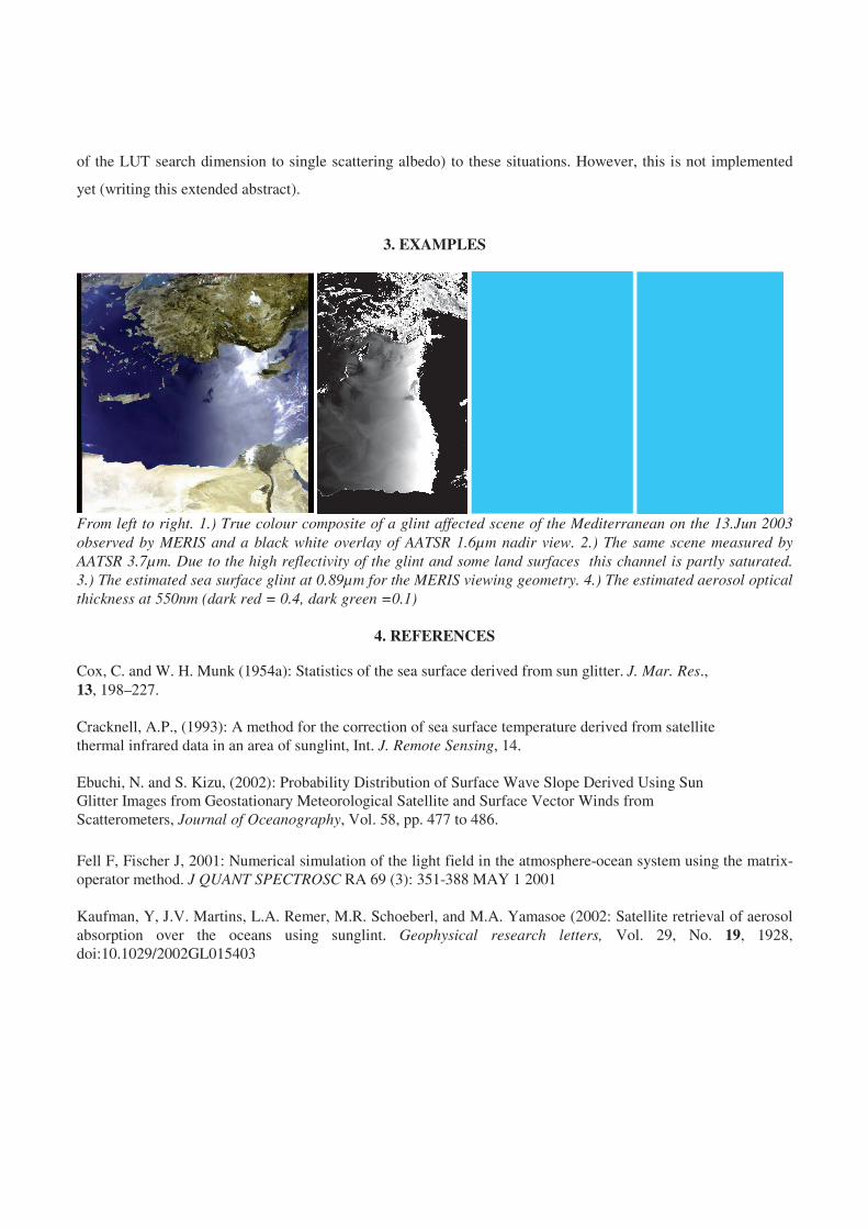
From left to right. 1.) True colour composite of a glint affected scene of the Mediterranean on the 13.Jun 2003 observed by MERIS and a black white overlay of AATSR 1.6 m nadir view. 2.) The same scene measured by AATSR 3.7 m. Due to the high reflectivity of the glint and some land surfaces this channel is partly saturated. 3.) The estimated sea surface glint at 0.89 m for the MERIS viewing geometry. 4.) The estimated aerosol optical thickness at 550nm (dark red = 0.4, dark green =0.1)

4. REFERENCES

Cox, C. and W. H. Munk (1954a): Statistics of the sea surface derived from sun glitter. J. Mar. Res., 13, 198–227.

Cracknell, A.P., (1993): A method for the correction of sea surface temperature derived from satellitethermal infrared data in an area of sunglint, Int. J. Remote Sensing, 14.

Ebuchi, N. and S. Kizu, (2002): Probability Distribution of Surface Wave Slope Derived Using Sun Glitter Images from Geostationary Meteorological Satellite and Surface Vector Winds from Scatterometers, Journal of Oceanography, Vol. 58, pp. 477 to 486.

Fell F, Fischer J, 2001: Numerical simulation of the light field in the atmosphere-ocean system using the matrix-operator method. J QUANT SPECTROSC RA 69 (3): 351-388 MAY 1 2001

Kaufman, Y, J.V. Martins, L.A. Remer, M.R. Schoeberl, and M.A. Yamasoe (2002: Satellite retrieval of aerosol absorption over the oceans using sunglint. Geophysical research letters, Vol. 29, No. 19, 1928, doi:10.1029/2002GL015403