aerodynamics for engineers 5th edition
TRANSCRIPT


Conversion Factors
Density:
1.00 kg/rn3 1.9404 X slug/ft3 6.2430 X ibm/ft3
1.00 ibm/ft3 3.1081 X slug/ft3 = 16.018 kg/rn3
Energy or work:
1.00 cal = 4.187 J = 4.187 N rn1.00 Btu = 778.2 ft lbf 0.2520 kcal = 1055 J
1.00 kW h = 3.600 x j
Flow rates:
Force:
1.00 gal/mm = 6.309 X m3/s = 2.228 X ft3/s
Length:
Mass:
Power:
1.00 N
1.00 lbf
1.00 lhf
1.00 U.S. ton
1.00 W/cm2
= 3.170 x
1.OOm
1.00 km
1.00 ft
1.00 ft
1.00 mile =
1.00 kg
1.00 slug =
1.00kW
1.00 kW
1.00 hp
1.00 Btu/s
1.00 Btu/h
= dyne = 0.2248 lbf
= 4.4482 N
16.0 oz
= 2000 lbf 2.0 kip
0,2388 cal/s cm2 = 0.8806 Btu/ft2. s
But/ft2. h
= 3.2808 ft = 39.37 in.
= 0.6214 mile = 1093.6 yd
= 0.3048 m = 30.48 cm
= 12 in = 0.333 yd
5280 ft 1760yd = 1609.344m
1000 g = 2.2047 ibm
32,174 ibm 14.593 kg
= 1000.0 W = 1000.0 N rn/s = 0.2388 kcal/s
= 1.341 hp
550 ft lbf/s = 0.7457 kW
= 1.415 hp
= 0.29307 W
Heat flux:
Pressure:
1.00 N/rn2 = 1.4504 X lbf/in.2 2.0886 X 10² lbf/ft21.00 bar = N/rn2 = Pa1.00 lbf/in.2 = 6.8947 X N/rn2
1.00 lbf/in.2 = 144.00 lbf/ft2
Specific enthalpy:
1.00 N rn/kg = 1.00 J/kg 1.00 rn2/s2
1.00 rn/kg = 4.3069 X Btu/lbm = 1.0781 ft lbf/slug1.00 Btu/lbrn = 2.3218 X N rn/kg
Specific heat:
1.00 N rn/kg. K = 1.00 J/kg - K = 2.388)< Btu/lbm °R= 5.979 ft . lbf/slug
1.00 Btu/lbm = 32.174 Btu/slug- = 4.1879 X N rn/kg. K= 4.1879 X 3/kg K
Temperature:The temperature of the ice point is 273.15 K (491.67°R).1.00 K = 1.80°R
K = °C + 273.15°R =°F+45967T°F = 1.8(T°C) + 32T°R = 1.8(T K)
Velocity:
1.00 rn/s = 3.60 km/h1.00 km/h = 0.2778 rn/s = 0.6214 mile/h = 0.9113 ft/s1.00 ft/s = 0.6818 mile/h = 0.59209 knot1.00 mile/h = 1.467 ft/s 1.609 km/h 0.4470 rn/s1.00 knot = 1.15155 mile/h
Viscosity:
1.00 kg/rn - s = 0.67197 ibm/ft s = 2.0886 X lbf- s/ft21.00 ibm/ft. s = 3.1081 X lbf' s/ft2 = 1.4882 kg/rn . s
1.00 lbf s/ft2 = 47.88 N - s/rn2 = 47.88 Pa s1.00 centipoise = 0.001 Pa s = 0.001 kg/rn. s = 6.7 197 X ibm/ft s1.00 stoke = 1.00 x rn2/s(kinematic viscosity)
Volume:
1.00 liter = 1000.0 crn3
1.00 barrel = 5.6146 ft3
1.00 ft3 = 1728 in.3 = 0.03704 yd3 = 7.481 gal= 28.32 liters
1.00 gal = 3.785 liters = 3.785 x m3
1.00 bushel = 3.5239 x 10⁻² rn3

AERODYNAMICSFOR ENGINEERS
Fifth Edition
JOHN J. BERTINProfessor Emeritus, United States Air Force Academy
and
RUSSELL M. CUMMINGSProfessor, United States Air Force Academy
PEARSON
Prentice
Pearson Education International

If you purchased this book within the United States or Canada you should be aware that it has been wrongfullyimported without the approval of the Publisher or the Author.
Vice President and Editorial Director, ECS: Marcia .1. HortonAcquisitions Editor: Tacy QuinnAssociate Editor: Dee BetnhardManaging Editor: Scott DisannoProduction Editor: Rose KernanArt Director: Kenny BeckArt Editor: Greg DuIlesCover Designer: Kristine CarneySenior Operations Supervisor: Alexis Heydt-LongOperations Specialist: Lisa McDowellMarketing Manager: Tim Galligan
Cover images left to right: Air Force B-lB Lancer Gregg Stansbery photo I Boeing Graphic based on photo and dataprovided by Lockheed Martin Aeronautics F-iS I NASA.
p EARSO N
Prentice© 2009,2002,1998,1989,1979 by Pearson Education, Inc.Pearson Prentice-HallUpper Saddle River, NJ 07458
All rights reserved. No part of this book may be reproduced in any form or by any means, without permission in writingfrom the publisher.The author and publisher of this book have used their best efforts in preparing this book.These effortsinclude the development, research, and testing of the theories and programs to determine their effectiveness. The authorand publisher make no warranty of any kind, expressed or implied, with regard to these programs or the documentationcontained in this book.The author and publisher shall not be liable in any event for incidental or consequential damagesin connection with, or arising out of these programs.
ISBN-10: 0-13-235521-3ISBN-13:Printed in the United States of America10 9 8 7 6 5 4 3 2 1
Pearson Education Ltd., LondonPearson Education Singapore, Pte. LtdPearson Education Canada, Inc.Pearson Education—JapanPearson Education Australia PTY, LimitedPearson Education North Asia, Ltd., Hong KongPearson Educación de Mexico, S.A. de CV.Pearson Education Malaysia, Pte. Ltd.Pearson Education Upper Saddle River, New Jersey
Contents
PREFACE TO THE FIFTH EDITION 15PREFACE TO THE FOURTH EDITION 17
CHAPTER 1 WHY STUDY AERODYNAMICS? 21
1.1 The Energy-Maneuverability Technique 211.1.1 Specific Excess Power 241.1.2 Using Specific Excess Power to Change
the Energy Height 251.1.3 John K Boyd Meet Harry Hillaker 26
1.2 Solving for the AerothermodynamicParameters 261.2.1 Concept of a Fluid 271.2.2 Fluid as a Continuum 271.23 Fluid Properties 281.2.4 Pressure Variation in a Static Fluid Medium 341.2.5 The Standard Atmosphere 39
1.3 Summary 42
Problems 42References 47
CHAPTER 2 FUNDAMENTALS OF FLUID MECHANICS 48
2.1 Introduction to Fluid Dynamics 492.2 Conservation of Mass 512.3 Conservation of Linear Momentum 542.4 Applications to Constant-Property Flows 592.5 Reynolds Number and Mach Number as
Similarity Parameters 652.6 Concept of the Boundary Layer 692.7 Conservation of Energy 722.8 First Law of Thermodynamics 722.9 Derivation of the Energy Equation 74
2.9.1 Integral Form of the Energy Equation 772.9.2 Energy of the System 78
5
Contents
2.9.3 Flow Work 782.9.4 Viscous Work 792.9.5 Shaft Work 802.9.6 Application of the Integral Form
of the Energy Equation 80
2.10 Summary 82
Problems 82Ref erences 93
CHAPTER 3 DYNAMICS OF AN INCOMPRESSIBLE,INVISCID FLOW FIELD 94
3.1 Inviscid Flows 943.2 Bernoulli's Equation 953.3 Use of Bernoulli's Equation
to Determine Airspeed 983.4 The Pressure Coefficient 1013.5 Circulation 1033.6 Irrotational Flow 1053.7 Kelvin's Theorem 106
3.7.1 Implication of Kelvin Theorem 107
3.8 Incompressible, Irrotational Flow 1083.&1 Boundary Conditions 108
3.9 Stream Function in a Two-Dimensional,Incompressible Flow 108
3.10 Relation Between Streamlines and EquipotentialLines 110
3.11 Superposition of Flows 1133.12 Elementary Flows 113
3.12.1 Uniform Flow 1133.12.2 Source or Sink 1143.12.3 Doublet 1163.12.4 Potential Vortex 1173.12.5 Summary of Stream Functions
and of Potential Functions 119
3.13 Adding Elementary Flows to Describe FlowAround a Cylinder 1193.13.1 Velocity Field 1193.13.2 Pressure Distribution 1223.13.3 Lift and Drag 125
3.14 Lift and Drag Coefficients as DimensionlessFlow-Field Parameters 128
3.15 Flow Around a Cylinder with Circulation 1333.15.1 Velocity Field 1333.15.2 Lift and Drag 133
Contents
3.16 Source Density Distributiononthe Body Surface 135
3.17 Incompressible, Axisymmetric Flow 1403.17.1 Flow around a Sphere 141
3.18 Summaiy 143
Problems 144References 157
CHAPTER 4 VISCOUS BOUNDARY LAYERS 158
4.1 Equations Governing the Boundary Layerfor a Steady, Two-Dimensional, IncompressibleFlow 159
4.2 Boundary Conditions 1624.3 Incompressible, Laminar Boundary Layer 163
4.3.1 Numerical Solutions for the Falkner-SkanProblem 166
4.4 Boundary-Layer Transition 1804.5 Incompressible, Turbulent Boundary Layer 183
4.5.1 Derivation of the Momentum Equationfor Turbulent Boundary Layer 184
4.5.2 Approaches to Turbulence Modeling 187Turbulent Boundary Layer for a Flat Plate 188
4.6 Eddy Viscosity and Mixing Length Concepts 1914.7 Integral Equations for a Flat-Plate Boundary
Layer 1934.7.1 Application of the Integral Equations of Motion
to a Turbulent, Flat-Plate Boundary Layer 1964.7.2 Integral Solutions for a Turbulent Boundary
Layer with a Pressure Gradient 202
4.8 Thermal Boundary Layer for Constant-PropertyFlows 2034.8.1 Reynolds Analogy 2054.8,2 Thermal Boundary Layer for Pr 1 206
4.9 Summary 210
Problems 210References 214
CHAPTER 5 CHARACTERISTIC PARAMETERS FOR AIRFOILAND WING AERODYNAMICS 215
5.1 Characterization of Aerodynamic Forcesand Moments 2155.1.1 General Comments 2155.1.2 Parameters That Govern Aerodynamic Forces 218
Contents
5.2 Airfoil Geometry Parameters 2195.2.1 Airfoil-Section Nomenclature 2195.2.2 Leading-Edge Radius and Chord Line 2205.2.3 Mean Camber Line 2205.2,4 Maximum Thickness and Thickness
Distribution 2215.2.5 Trailing-Edge Angle 222
5.3 Wing-Geometry Parameters 2225.4 Aerodynamic Force and Moment
Coefficients 2295.4.1 Lift Coefficient 2295.4.2 Moment Coefficient 2345.4.3 Drag Coefficient 2365.4.4 Boundary-Layer Transition 2405.4.5 Effect of Surface Roughness on
the Aerodynamic Forces 2435.4.6 Method for Predicting Aircraft Parasite
Drag 246
5.5 Wings of Finite Span 2565.5.1 Lift 2575.5.2 Drag 2605.5.3 Lift/Drag Ratio 264
Problems 269References 273
CHAPTER 6 INCOMPRESSIBLE FLOWS AROUND AIRFOILSOF INFINITE SPAN 275
6.1 General Comments 2756.2 Circulation and the Generation of Lift 276
6.2.1 Starting Vortex 277
6.3 General Thin-Airfoil Theory 2786.4 Thin, Flat-Plate Airfoil (Symmetric Airfoil) 2816.5 Thin, Cambered Airfoil 285
6.5.1 Vorticity Distribution 2866.5.2 Aerodynamic Coefficients for a Cambered
Airfoil 287
6.6 Laminar-Flow Airfoils 2946.7 High-Lift Airfoil Sections 2996.8 Multielement Airfoil Sections for Generating
High Lift 3046.9 High-Lift Military Airfoils 312
Problems 314References 316
Contents
CHAPTER 7 INCOMPRESSIBLE FLOW -
ABOUT WINGS OF FINITE SPAN 319
7.1 General Comments 3197.2 Vortex System 3227.3 Lifting-Line Theory for Unswept Wings 323
7.3.1 TrailingVortices and Down wash 3267.3.2 Case of Elliptic Spanwise circulation
Distribution 3287.3.3 Technique for General Spanwise Circulation
Distribution 3337.3.4 LiftontheWing 3397.3.5 Vortex-Induced Drag 339Z3.6 Some Final Comments on Lifting-Line Theory 346
7.4 Panel Methods 3497.4.1 Boundary Conditions 3507.4.2 Methods 351
7.5' Vortex Lattice Method 3527.5.1 Velocity Induced by a General Horseshoe
Vortex 3567.5.2 Application of the Boundary Conditions 3607.5.3 Relations for a Planar Wing 362
7.6 Factors Affecting Drag Due-to-Lift at SubsonicSpeeds 374
7.7 Delta Wings 3777.8 Leading-Edge Extensions 3877.9 Asymmetric Loads on the Fuselage at High
Angles of Attack 3917.9.1 Asymmetric Vortex Shedding 3927.9.2 Wakelike Flows 394
7.10 Flow Fields For Aircraft at High Anglesof Attack 394
7.11 Unmanned Air Vehicle Wings 3967.12 Summary 398
Problems 399References 400
CHAPTER 8 DYNAMICS OF A COMPRESSIBLE FLOW FIELD 404
8.1 Thermodynamic Concepts 4058.1.1 Specific Heats 4058.1.2 Additional Relations 407&1.3 Second Law of Thermodynamics
and Reversibility 4088.1.4 Speed of Sound 410
8.2 Adiabatic Flow in a Variable-AreaStreamtube 412
Contents
8.3 Isentropic Flow in a Variable-AreaStreamtube 417
8.4 Characteristic Equations and Prandtl-MeyerFlows 422
8.5 Shock Waves 4308.6 Viscous Boundary Layer 440
8.6.1 Effects of Compressibility 442
8.7 The Role of Experiments for GeneratingInformation Defining the Flow Field 4468.7.1 Ground-Based Tests 4468.7.2 Flight Tests 450
8.8 Comments About The Scaling/CorrectionProcess(Es) For Relatively Clean CruiseConfigurations 455
8.9 Shock-Wave/Boundary-Layer Interactions 455
Problems 457References 464
CHAPTER 9 COMPRESSIBLE, SUBSONIC FLOWSAND TRANSONIC FLOWS 467
9.1 compressible, Subsonic Flow 468.1.1 Linearized Theory for Compressible Subsonic
Flow About a Thin Wing at Relatively SmallAngles of Attack 468
9.2 Transonic Flow Past Unswept Airfoils 4739.3 Wave Drag Reduction by Design 482
9.3.1 Airfoil Contour Wave Drag Approaches 4829.3.2 Supercritical Airfoil Sections 482
9.4 Swept Wings at Transonic Speeds 4849.4.1 Wing—Body Interactions and the "Area Rule" 4869.4.2 Second-Order Area-Rule 4949.4.3 Forward Swept Wing 497
9.5 Transonic Aircraft 5009.6 Summary 503
Problems 503References 504
CHAPTER 10 TWO-DIMENSIONAL, SUPERSONIC FLOWSAROUND THIN AIRFOILS 507
10.1 Linear Theory 50810.1.1 Lift 50910.1.2 Drag 51210.1.3 Pitching Moment 513
Contents
10.2 Second-Order Theory (Busemann's Theory) 51610.3 Shock-Expansion Technique 519
Problems 524References 527
CHAPTER 11 SUPERSONIC FLOWS OVER WINGS AND AIRPLANECONFIGURATIONS 528
11.1 General Remarks About Lift and Drag 53011.2 General Remarks About Supersonic Wings 53111.3 Governing Equation and Boundary
Conditions 53311.4 Consequences of Linearity 53511.5 Solution Methods 53511.6 Conical-Flow Method 536
11.6.1 Rectangular Wings 53711.6.2 Swept Wings 54211.6.3 Delta and Arrow Wings 546
11.7 Singularity-Distribution Method 54811.7.1 Find the Pressure Distribution Given the
configuration sso11.7.2 Numerical Method for Calculating the Pressure
Distribution Given the Configuration 55911.7.3 Numerical Method for the Determination of
Camber Distribution 572
11.8 Design Considerations for SupersonicAircraft 575
11.9 Some-Comments About the Design of the SSTand of the HSCT 5791L9.1 The Supersonic Transport
the Concorde 57911.9.2 The High-Speed civil Transport (HSCT) 58011.9.3 Reducing the Sonic Boom 58011.9.4 Classifying High-Speed Aircraft Designs 582
11.10 Slender Body Theory 58411.11 Aerodynamic Interaction 58711.12 Aerodynamic Analysis for Complete
Configurations in a Supersonic Stream 590
Problems 591References 593
CHAPTER 12 HYPERSONIC FLOWS 596
12.1 Newtonian Flow Model 59712.2 Stagnation Region Flow-Field Properties 600
Contents
12.3 Modified Newtonian Flow 60512.4 High LID Hypersonic Configurations —
Waveriders 62112.5 Aerodynamic Heating 628
12.5.1 Similarity Solutions for Heat Transfer 632
12.6 A Hypersonic Cruiser for the Twenty-FirstCentury? 634
12.7 Importance of Interrelating CFD, Ground-TestData, and Flight-Test Data 638
12.8 Boundary-Layer Transition Methodology 640
Problems 644References 646
CHAPTER 13 AERODYNAMIC DESIGN CONSIDERATIONS 649
13.1 High-Lift Configurations 64913.1.1 Increasing the Area 65013.1.2 Increasing the Lift Coefficient 65113.1.3 Flap Systems 65213.1.4 Multielement Airfoils 65613.1.5 Power-Augmented Lift 659
13.2 Circulation Control Wing 66313.3 Design Considerations For Tactical Military
Aircraft 66413.4 Drag Reduction 669
13.4.1 Variable- Twist, Variable-Camber Wings 66913.4.2 Laminar-Flow Control 67013.4.3 Wingtip Devices 67313.4.4 Wing Planform 676
13.5 Development of an Airframe Modificationto Improve the Mission Effectiveness ofan Existing Airplane 67813.5.1 The EA-6B 67813.12 The Evolution of the F-16 68113.5.3 External Carriage of Stores 68913.5.4 Additional Comments 694
13.6 Considerations for Wing/Canard, Wing/Tail,and Tailless Configurations 694
13.7 Comments on the F-iS Design 69913.8 The Design of the F-22 70013.9 The Design of the F-35 703
Problems 706References 708
Contents 13
CHAPTER 14 TOOLS FOR DEFININGTHE AEROD YNA MI C ENVIRONMENT 711
14.1 CFD Tools 71314.1.1 Semiempirical Methods 71314.1.2 Surface Panel Methods for Inviscid Flows 71414.1.3 Euler Codes for Inviscid Flow Fields 71514.1.4 Two-LayerFlowModels 71514.1.5 Computational Techniques that Treat the Entire
Flow Field in a Unified Fashion 71614.1.6 Integrating the Diverse CFD Tools 717
14.2 Establishing the Credibility of CFDSimulations 718
14.3 Ground-Based Test Programs 72014.4 Flight-Test Programs 72314.5 Integration of Experimental and Computational
Tools: The Aerodynamic Design Philosophy 724
References 725
APPENDIX A THE EQUATIONS OF MOTION WRITTENIN CONSERVATION FORM 728
APPENDIX B A COLLECTION OF OFTEN USED TABLES 734
INDEX 742

Preface to theFifth Edition
There were two main goals for writing the Fifth Edition of Aerodynamics for Engineers:1) to provide readers with a motivation for studying aerodynamics in a more casual, en-joyable, and readable manner, and 2) to update the technical innovations and advance-ments that have taken place in aerodynamics since the writing of the previous edition.
To help achieve the first goal we provided readers with background for the truepurpose of aerodynamics. Namely, we believe that the goal of aerodynamics is to pre-dict the forces and moments that act on an airplane in flight in order to better under-stand the resulting performance benefits of various design choices. In order to betteraccomplish this, Chapter 1 begins with a fun, readable, and motivational presentation onaircraft performance using material on Specific Excess Power (a topic which is taughtto all cadets at the U.S. Air Force Academy). This new introduction should help to makeit clear to students and engineers alike that understanding aerodynamics is crucial to un-derstanding how an airplane performs, and why one airplane may 'be better than an-other at a specific task.
Throughout the remainder of the fifth edition we have added new and emerging air-craft technologies that relate to aerodynamics. These innovations include detailed dis-cussion about laminar flow and low Reynolds number airfoils, as well as modern high-liftsystems (Chapter 6); micro UAV and high altitude/lông endurance wing geometries(Chapter 7); the role of experimentation in determining aerodynamics, including the im-pact of scaling data for full-scale aircraft (Chapter 8); slender-body theory and sonicboom reduction '(Chapter 11); hypersonid transition (Chapter 12); and wing-tip devices,as well as modern wing planforms (Chapter 13). Significant new material on practicalmethods for estimating aircraft drag have also been incorporated into Chapters 4 and 5,including methods for' estimating skin friction, form' factor, roughness effects, and the im-pactof boundary-layer transition. Of special interest in the fifth edition is a descriptionof the aerodynamic design of the F-35, now included in Chapter 13.
In addition, there are 32 new figures containing updated and new information, aswell as numerous, additional up-to-date references throughout the book. New problemshave been added to almost every chapter, as well as example problems showing studentshow the theoretical concepts can be applied to practical problems. Users of the fourth edi-tion of the book will find that all material included in that edition is still included in the
15
Preface to the Fifth Edition
fifth edition, with the new material added throughout the book to bring a real-world fla-vor to the concepts being developed. We hope that readers will find the incluslon of allof this additional material helpful and informative.
In order to help accomplish these goals a new co-author, Professor Russell M.Cummings of the U.S. Air Force Academy, has been added for the fifth edition ofAerodynamics for Engineers. Based on his significant contributions to both the writingand presentation of new and updated material, he makes a welcome addition to thequality and usefulness of the book.
Finally, no major revision of a book like Aerodynamics for Engineers can takeplace without the help of many people. The authors are especially indebted to everyonewho aided in collecting new materials for the fifth edition. We want to especially thankDoug McLean, John McMasters, and their associates at Boeing; Rick Baker, Mark Buch-holz, and their associates from Lockheed Martin; Charles Boccadoro, David Graham,and their associates of Northrop Grumman; Mark Drela, Massachusetts Institute ofTechnology; Michael Seig, University of Illinois; and Case van Darn, University of Cal-ifornia, Davis. In addition, we are very grateful for the excellent suggestions and com-ments made by the reviewers of the fifth edition: Doyle Knight of Rutgers University,Hui Hu of Iowa State University, and Gabriel Karpouzian of the U.S. Naval Academy.Finally, we also want to thank Shirley Orlofsky of the U.S. Air Force Academy for herunfailing support throughout this project.
Preface to theFourth Edition
This text is designed for use by undergraduate students in intermediate and advancedclasses in aerodynamics and by graduate students in mechanical engineering andaerospace engineering. Basic fluid mechanic principles are presented in the first fourchapters. Fluid properties and a model for the standard atmosphere are discussed inChapter 1, "Fluid Properties." The equations governing fluid motion are presented inChapter 2, "Fundamentals of Fluid Mechanics." Differential and integral forms ofthe continuity equation (based on the conservation of mass), the linear momentumequation (based on Newton's law of motion), and the energy equation (based on thefirst law of thermodynamics) are presented. Modeling inviscid, incompressible flowsis the subject of Chapter 3, "Dynamics of an Incompressible, Inviscid Flow Field."Modeling viscous boundary layers, with emphasis on incompressible flows, is the subjectof Chapter 4, "Viscous Boundary Layers." Thus, Chapters 1 through4 present mate-rial that covers the principles upon which the aerodynamic applications are based. Forthe reader who already has had a course (or courses) in fluid mechanics, these fourchapters provide a comprehensive review of fluid mechanics and an introduction tothe nomenclature and style of the present text.
At this point, the reader is ready to begin material focused on aerodynamic applica-tions. Parameters that characterize the geometry of aerodynamic configurations andparameters that characterize aerodynamic performance are presented in Chapter 5, "Char-acteristic Parameters for Airfoil and Wing Aerodynamics." Techniques for modeling theaerodynamic performance of two-dimensional airfoils and of finite-span wings at lowspeeds (where variations in density are negligible) are presented in Chapters 6 and7,respectively. Chapter 6 is titled "Incompressible Flows around Wings of Infinite Span,"and Chapter 7 is titled "Incompressible Flow about Wings of Finite Span."
The next five chapters deal with compressible flow fields. To provide the readerwith the necessary background for high-speed aerodynamics, the basic fluid mechanicprinciples for compressible flows are discussed in Chapter 8, "Dynamics of a Com-pressible Flow Field." Thus, from a pedagogical point of view, the material presented inChapter 8 complements the material presented in Chapters 1 through4. Techniques formodeling high-speed flows (where density variations cannot be neglected) are presentedin Chapters 9 throughl2. Aerodynamic performance for compressible, subsonic flows
17
Preface to the Fourth Edition
through transonic speeds is the subject of Chapter 9, "Compressible Subsonic Flowsand Transonic Flows." Supersonic aerodynamics for two-dimensional airfoils is thesubject of Chapter 10, "Two-Dimensional Supersonic Flows about Thin Airfoils" andfor finite-span wings in Chapter 11,"Supersonic Flows over Wings and Airplane Con-figurations." Hypersonic flowsare the subject of Chapter 12.
At this point, chapters have been dedicated to the development of basic models forcalculating the aerodynamic performance parameters for each of the possible speed ranges.The assumptions and, therefore, the restrictions incorporated into the development ofthe theory are carefully noted. The applications of the theory are illustrated by workingone or more problems. Solutions are obtained using numerical techniques in order to applythe theory for those flows where closed-form solutions are impractical or impossible. Ineach of the the computed aerodynamic parameters are compared with experi-mental data from the open literature to illustrate both the validity of the theoretical analy-sis and its limitations (or, equivalently, the range of conditions for which the theory isapplicable). One objective is to use the experimental data to determine the limits of applic-ability for the proposed models.
Extensive discussions of the effects of viscosity, compressibility, shock/boundary-layer interactions, turbulence modeling, and other practical aspects of contemporaryaerodynamic design are also presented. Problems at the end of each chapter are designedto complement the material presented within the chapter and to develop the student'sunderstanding of the relative importance of various phenomena. The text emphasizespractical problems and the techniques through which solutions to these problems canbe obtained. Because both the International System of Units (Système Internationald'Unitès, abbreviated SI) and English units are commonly used in the aerospace indus-try, both are used in this text. Conversion factors between SI units and English units arepresented on the inside covers.
Advanced material relating to design features of aircraft over more than a cen-tury and to the tools used to define the aerodynamic parameters are presented inChapters 13 andl4. Chapter 13 is titled "Aerodynamic Design Considerations," andChapter 14 is titled "Tools for Defining the Aerodynamic Environment." Chapter 14presents an explanation of the complementary role of experiment and of computa-tion in defining the aerodynamic environment. Furthermore, advantages, limita-tions, and roles of computational techniques of varying degrees of rigor are discussed.The material presented in Chapters 13 andl4 not only should provide interestingreading for the student but, should be useful to professionals long after they havecompleted their academic training.
COMMENTS ON THE FIRST THREE EDITIONS
The author would like to thank Michael L. Smith for his significant contributions toAerodynamics for Engineers. Michael Smith's contributions helped establish the quali-ty of the text from the outset and the foundation upon which the subsequent editionshave been based. For these contributions, he was recognized as coauthor of the firstthree editions.
The author is indebted to his many friends and colleagues for their help in preparingthe first three editions of this text. I thank for their suggestions, their support, and for
Preface to the Fourth Edition
copies of photographs, illustrations, and reference documents. The author is indebtedto L. C. Squire of Cambridge University; V. G. Szebehely of the University of Texas atAustin; F. A. Wierum of the Rice University; T. J. Mueller of the University of NotreDame; R. G. Bradley and C. Smith of General Dynamics; 0. E. Erickson of Northrop;L. E. Ericsson of Lockheed Missiles and Space; L. Lemmerman and A. S. W. Thomas ofLockheed Georgia; J. Periaux of Avions Marcel Dassault; H. W. Carison, M. L. Spearman,and P. E Covell of the Langley Research Center; D. Kanipe of the Johnson Space Center;R. C. Maydew, S. McAlees, and W H. Rutledge of the Sandia National Labs; M. J. Nipperof the Lockheed Martin Tactical Aircraft Systems; H. J. Hillaker (formerly) of GeneralDynamics; R. Chase of the ANSER Corporation; and Lt. Col. S. A. Brandt, Lt. Col.W. B. McClure, and Maj. M. C. Towne of the U.S. Air Force Academy. F. R. DeJarnetteof North Carolina State University, and J. F. Marchman III, of Virginia Polytechnic Insti-tute and State University provided valuable comments as reviewers of the third edition.
Not only has T. C. Valdez served as the graphics artist for the first three editionsof this text, but he has regularly located interesting articles on aircraft design thathave been incorporated into the various editions.
THE FOURTH EDITION
Rapid advances in software and hardware have resulted in the ever-increasing use ofcomputational fluid dynamics (CFD) in the design of aerospace vehicles. The increasedreliance on computational methods has led to three changes unique to the fourth edition.
1. Some very sophisticated numerical solutions for high alpha flow fields(Chapter 7), transonic flows around an NACA airfoil (Chapter 9), and flowover the SR-71 at three high-speed Mach numbers (Chapter 11) appear forthe first time in Aerodynamics for Engineers. Although these results haveappeared in the open literature, the high-quality figures were provided byCobalt Solutions, LLC, using the postprocessing packages Fieldview andEnSight. Captain J. R. Forsythe was instrumental in obtaining the appro-priate graphics.
2. The discussion of the complementary use of experiment and computation astools for defining the aerodynamic environment was the greatest single changeto the text. Chapter 14 was a major effort, intended to put in perspective thestrengths and limitations of the various tools that were discussed individuallythroughout the text.
3. A CD with complementary homework problems and animated graphics isavailable to adopters. Please contact the author at USAFA.
Major D. C. Blake, Capt. J. R. Forsythe, and M. C. Towne were valuable contribu-tors to the changes that have been made to the fourth edition.They served as soundingboards before the text was written, as editors to the modified text, and as suppliers ofgraphic art. Since it was the desire of the author to reflect the current role of computa-tions (limitations, strengths, and usage) and to present some challenging applications, theauthor appreciates the many contributions of Maj. Blake, Capt. Forsythe, and Dr. Towne,who are active experts in theuse and in the development of CFD in aerodynamic design.
20 Preface to the Fourth Edition
The author would also like to thank M. Gen. E. R. Bracken for supplying in-formation and photographs regarding the design and operation of military aircraft.G. E. Peters of the Boeing Company and M. C. Towne of Lockheed Martin Aero-nautics served as points of contact with their companies in providing material new tothe fourth edition.
The author would like to thank John Evans Burkhalter of Auburn University,Richard S. Figliola of Clemson University, Marilyn Smith of the Georgia Institute ofTechnology, and Leland A. Carlson of Texas A & M University, who, as reviewers of adraft manuscript, provided comments that have been incorporated either into the textor into the corresponding CD.
The author would also like to thank the American Institute of Aeronautics andAstronautics (AJAA), the Advisory Group for Aerospace Research and Development,North Atlantic Treaty Organization (AGARD/NATO),1 the Boeing Company, and theLockheed Martin Tactical Aircraft System for allowing the author to reproduce sig-nificant amounts of archival material. This material not only constitutes a critical partof the fourth edition, but it also serves as an excellent foundation upon which the readercan explore new topics.
Fmally, thank you Margaret Baker and Shirley Orlofsky.
JOHN J. BERTINUnited States Air Force Academy
1The AGARD/NATO material was first published in the following publications: Conf Proc. High LiftSystem Aerodynamics, CP-515, Sept. 1993; Gonf Proc. Vèilidation of ('omputational Fluid Dynamics, CV-437,vol.1, Dec.1988; Report, Special Course on Aerothermodynamics of Hypersonic Vehicles, R-761, June 1989.
1 WHY STUDY
AERODYNAMICS?
1.1 THE ENERGY-MANEUVERABILITY TECHNIQUE
Early in the First World War, fighter pilots (at least those good enough to survive theirfirst engagements with the enemy) quickly developed tactics that were to serve themthroughout the years. German aces, such as Oswald Boelcke and Max Immelman, real-ized that, if they initiated combat starting from an altitude that was greater than that oftheir adversary, they could dive upon their foe, trading potential energy (height) for ki-netic energy (velocity). Using the greater speed of his airplane to close from the rear (i.e.,from the target aircraft's "six o'clock position"), the pilot of the attacking aircraft coulddictate the conditions of the initial phase of the air-to-air combat. Starting from a supe-rior altitude and converting potential energy to kinetic energy, the attacker might beable to destroy his opponent on the first pass. These tactics were refined, as the suc-cessful fighter aces gained a better understanding of the nuances of air combat by build-ing an empirical data base through successful air-to-air battles. A language grew up tocodify these tactics: "Check your six."
This data base of tactics learned from successful combat provided an empiricalunderstanding of factors that are important to aerial combat. Clearly, the sum of the po-tential energy plus the kinetic energy (i.e., the total energy) of the aircraft is one of thefactors.
21
22 Chap. '1 / Why Study Aerodynamics?
EXAMPLE Li: The total energy
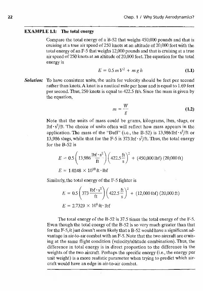
Compare the total energy of a B-52 that weighs 450,000 pounds and that iscruising at a true air speed of 250 knots at an altitude of 20,000 feet with thetotal energy of an F-S that weighs 12,000 pounds and that is cruising at a trueair speed of 250 knots at an altitude of 20,000 feet. The equation for the totalenergy is
E = 0.5mV2 + mgh
Solution: To have consistent units, the units for velocity should be feet per secondrather than knots. A knot is a nautical mile per hour and is equal to 1.69 feetper second. Thus, 250 knots is equal to 422.5 ft/s. Since the mass is given bythe equation,
wg
Note that the units of mass could be grams, kilograms, ibm, slugs, ors2/ft. The choice of units often will reflect how mass appears in the
application. The mass of the "Buff" (i.e., the B-52) is 13,986 lbf s2/ft or13,986 slugs, while that for the F-S is 373 lbf- s2/ft. Thus, the total energyfor the B-52 is
E = 0.5(139861bf.s2)
+ (450,000 lbf) (20,000ft)
E = 1.0248 X 1010 ft ibf
Similarly, the total energy of the F-S fighter is
= 0.5 (373 lbf s2)(422.5 + (12,000 lbf) (20,000
E = 2.7329 x 108 ft lbf
The total energy of the B-52 is 37.5 times the total energy of the F-S.Even though the total energy of the B-52 is so very much greater than thatfor the F-5, it just doesn't seem likely that a B-52 would have a significant ad-vantage in air-to-air combat with an F-S. Note that the two aircraft are cruis-ing at the same ifight condition (velocity/altitude combination). Thus, thedifference in total energy is in direct proportion to the difference in theweights of the two aircraft. Perhaps the specific energy (i.e., the energy perunit weight) is a more realistic parameter when trying to predict which air-craft would have an edge in air-to-air combat.
Sec. Li I The Energy-Maneuverability Technique 23
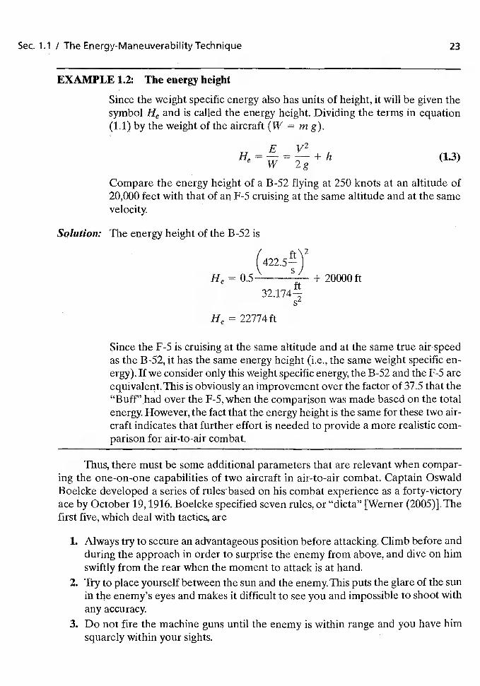
EXAMPLE 1.2: The energy height
Since weight specific energy also has units of height, it will be given thesymbol and is called the energy height. Dividing the terms in equation(1.1) by the weight of the aircraft (W in g).
E v2W 2g
Compare the energy height of a B-52 flying at 250 knots at an altitude of20,000 feet with that of an F-5 cruising at the same altitude and at the samevelocity.
Solution: The energy height of the B-52 is
(422.5
He = 0.5 + 20000 ft
He = 22774 ft
Since the F-5 is cruising at the same altitude and at the same true air speedas the B-52, jt has the same energy height (i.e., the same weight specific en-ergy). If we consider only this weight specific energy, the 18-52 and the F-S areequivalent. This is obviously an improvement over the factor of 37.5 that the"Buff" had over the F-5,when the comparison was made based on the totalenergy. However, the fact that the energy height is the same for these two air-craft indicates that further effort is needed to provide a more realistic com-parison for air-to-air combat.
Thus, there must be some additional parameters that are relevant when compar-ing the one-on-one capabilities of two aircraft in air-to-air combat. Captain OswaldBoelcke developed a series of rules: based on his combat experience as a forty-victoryace by October 19, 1916. Boelcke specified seven rules, or "dicta" [Werner (2005)]. Thefirst five, which deal with tactics, are
1. Always try to secure an advantageous position before attacking. Climb before andduring the approach in order to surprise the enem.y from above, and dive on himswiftly from the rear when the moment to attack is at hand.
2. Try to place yourself between the sun and the enemy. This puts the glare of the sunin the enemy's eyes and makes it difficult to see you and impossible to shoot withany accuracy.
3. Do not fire the machine guns until the enemy is within range and you have himsquarely within your sights.
24 Chap. 1 / Why Study Aerodynamics?
4. Attack when the enemy least expects it or when he is preoccupied with otherduties, such as observation, photography, or bombing.
5. Never turn your back and try to run away from an enemy fighter. If you are sur-prised by an attack on your tail, turn and face the enemy with your guns.
Although Boelcke's dicta were to guide fighter pilots for decades to come, they wereexperienced-based empirical rules. The first dictum deals with your total energy, thesum of the potential energy plus the kinetic energy. We learned from the first two ex-ample calculations that predicting the probable victor in one-on-one air-to-air com-bat is not based on energy alone.
Note that the fifth dictum deals with maneuverability. Energy AND Maneuverability!The governing equations should include maneuverability as well as the specific energy.
It wasn't until almost half a century later that a Captain in the U.S. Air Forcebrought the needed complement of talents to bear on the problem [Coram (2002)]. Cap-tain John R. Boyd was an aggressive and talented fighter pilot who had an insatiable in-tellectual curiosity for understanding the scientific equations that had to be the basis ofthe "Boelcke dicta". John R. Boyd was driven to understand the physics that was thefoundation of the tactics that, until that time, had been learned by experience for thefighter pilot lucky enough to survive his early air-to-air encounters with an enemy. In hisrole as Director of Academics at the U.S. Air Force Fighter Weapons School, it becamenot only his passion, but his job.
Air combat is a dynamic ballet of move and countermove that occurs over a contin-uum of time. Thus, Boyd postulated that perhaps the time derivatives of the energy heightare more relevant than the energy height itself. How fast can we, in the target aircraft, withan enemy on our six, quickly dump energy and allow the foe to pass? Once the enemy haspassed, how quickly can we increase our energy height and take the offensive? John R.Boyd taught these tactics in the Fighter Weapons School. Now he became obsessed with thechallenge of developing the science of fighter tactics.
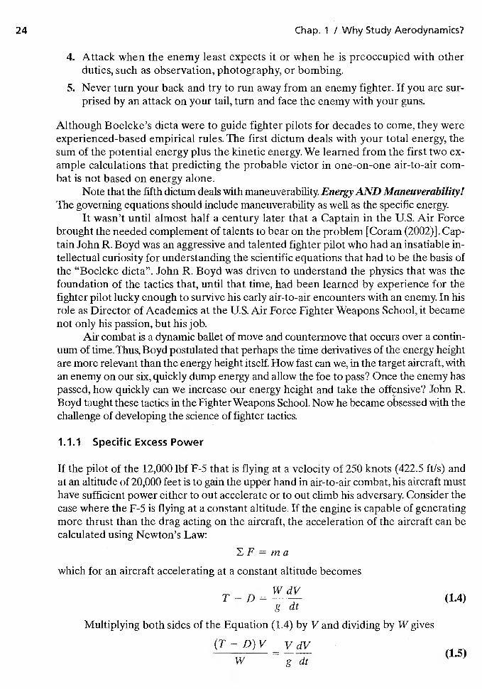
1.1.1 Specific Excess Power
If the pilot of the 12,000 lbf F-5 that is flying at a velocity of 250 knots (422.5 ft/s) andat an altitude of 20,000 feet is to gain the upper hand in air-to-air combat, his aircraft musthave sufficient power either to out accelerate or to out climb his adversary. Consider thecase where the F-5 is flying at a constant altitude. If the engine is capable of generatingmore thrust than the drag acting on the aircraft, the acceleration of the aircraft can becalculated using Newton's Law:
F ru a
which for an aircraft accelerating at a constant altitude becomes
(1.4)g dt
Multiplying both sides of the Equation (1.4) by V and dividing by W gives
(T—D)VVdV15
W gdt (.)
Sec. 1.1 / The Energy-Maneuverability Technique 25
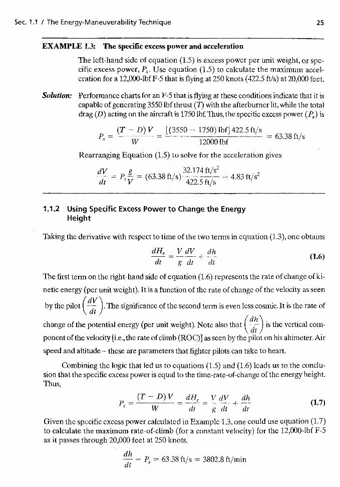
EXAMPLE 1.3: The specific excess power and acceleration
The left-hand side of equation (1.5) is excess power per unit weight, or spe-cific excess power, Use equation (1.5) to calculate the maximum accel-eration for a 12,000-lbf F-5 that is flying at 250 knots (422.5 ft/s) at 20,000 feet.
Performance charts for an F-S that is flying at these conditions indicate that it iscapable of generating 3550 lbf thrust (I) with the afterburner lit, while the totaldrag (D) acting on the aircraft is 1750 lbf.Thus, the specific excess power (Ps) is
(T — D) V [(3550 — 1750) lbf] 422.5 ft/s
= W 12000 lbf= 63.38 ft/s
Rearranging Equation (1.5) to solve for the acceleration gives
dV 32.174 ft/s2= = (63.38 ft/s)
422.5 ft/s= 4.83 ft/s
1.1.2 Using Specific Excess Power to Change the EnergyHeight
Taking the derivative with respect to time of the two terms in equation (1.3), one obtains
dHeVdV dhdt — g di' + dt
The first term on the right-hand side of equation (1.6) represents the rate of change of ki-
netic energy (per unit weight). It is a function of the rate of change of the velocity as seen
(dV'\ .by the pilot The significance of the second tenn is even less cosmic. It is the rate of
change of the potential energy (per unit weight). Note also that is the vertical com-
ponent of the velocity [i.e., the rate of climb (ROC)] as seen by the pilot on his altimeter. Air
speed and altitude — these are parameters that fighter pilots can take to heart.
Combining the logic that led us to equations (1.5) and (1.6) leads us to the conclu-sion that the specific excess power is equal to the time-rate-of-change of the energy height.Thus,
(T—D)V dHe VdV dhPs= =—=-——+—
W dt gdt di'
Given the specific excess power calculated in Example 1.3, one could use equation (1.7)to calculate the maximum rate-of-climb (for a constant velocity) for the 12,000-lbf F-Sas it passes through 20,000 feet at 250 knots.
= = 63.38 ft/s = 3802.8 ft/mm
26 Chap. 1 I Why Study Aerodynamics?
Clearly, to be able to generate positive values for the terms in equation (1.7), weneed an aircraft with excess power (i.e., one for Which the thrust exceeds the drag).Weight is another important factor, since the lighter the aircraft, the greater the bene-fits of the available excess power.
"Boyd, as a combat pilot in Korea and as a tactics instructor at Nellis AFB in theNevada desert, observed, analyzed, and assimilated the relative energy states of his aircraftand those of his opponent's during air combat engageinents... He also noted that, whenin a position of advantage, his energy was higher than that of his opponentand that he lostthat advantage when he allowed his energy to decay to less than that of his opponent."
"He knew that, when turning from a steady—state flight condition, the airplaneunder a given power setting would either slow down, lose altitude, or both. The resultmeant he was losing energy (the drag exceeded the thrust available from the engine).From these observations, he conclUded that maneuvering for position was basically anenergy problem. Winning required the proper management of energy available at theconditions existing at any point during a combat engagement." [Hillaker (1997)]
In the mid 1960s, Boyd had gathered energy-maneuverability data on all of thefighter aircraft in the U.S. Air Force inventory and on their adversaries. He sought to un-derstand the intricacies of maneuvering flight. What was it about the airplane that wouldlimit or prevent him from making it do what he wanted it to do?
1.1.3 John R. Boyd Meet Harry Hillaker
The relation between John R. Boyd and Harry Hillaker "dated from an evening in themid-1960s when a General Dynamics engineer named Harry Hillaker was sitting in theOfficer's Club at Eglin AFB, Florida, having an after dinner drink. Hillaker's host in-troduced him to a tall, blustery pilot named John R. Boyd, who immediately launcheda frontal attack on GD's F-ill fighter. Hillaker was annoyed but bantered back." [Grier(2004)] Hillaker countered that the F-ill was designated a fighter-bomber.
"A few days later, he (Hillaker) received a call—Boyd had been impressed byHillaker's grasp of aircraft conceptual design and wanted to know if Hillaker was in-terested in more organized meetings."
"Thus was born a group that others in the Air Force dubbed the 'fightcr mafia.'Their basic belief was that fighters did not need to overwhelm opponents with speedand size. Experience in Vietnam against nimble Soviet-built MiGs had convinced themthat technology had not yet turned air-to-air combat into a long-range shoot-out."[Grier (2004)]
The fighter mafia knew that a small aircraft could enjoy a high thrust-to-weightratio. Small aircraft have less drag. "The original F-16 design had about one-third the dragof an F-4 in level flight and one-fifteenth the drag of an F-4 at a high angle-of-attack."
1.2 SOLVING FOR THE AEROTHERMODYNAMIC PARAMETERS
A fundamental problem facing the aerodynamicist is to predict the aerodynamic forcesand moments and the heat-transfer rates acting on a vehicle in flight. In order to pre-dict these aerodynamic forces and moments with suitable accuracy, it is necessary to be
Sec. 1.2 / Solving for the Aerothermodynamic Parameters 27
able to describe the pattern of flow around the vehicle. The resultant flow pattern de-pends on the geometry of the vehicle, its orientation with respect to the undisturbedfree stream, and the altitude and speed at which the vehicle is traveling. In analyzing thevarious flows that an aerodynamicist may encounter, assumptions aboutthe fluid prop-erties may be introduced. In some applications, the temperature variations are so smallthat they do not affect the velocity field. In addition, for those applications where the tem-perature variations have a negligible effect on the flow field, it is often assumed thatthe density is essentially constant. However, in analyzing high-speed flows, the densityvariations cannot be neglected. Since density is a function of pressure and temperature,it may be expressed in terms of these two parameters. In fact, for a gas in thermody-namic equilibrium, any thermodynamic property may be expressed as a function of twoother independent, thermodynamic properties. Thus, it is possible to formulate the gov-erning equations using the enthalpy and the entropy as the flow properties instead of thepressure and the temperature.
1.2.1 Concept of a Fluid
From the point of view of fluid mechanics, matter can be in one of two states, eithersolid or fluid. The technical distinction between these two states lies in their response toan applied shear, or tangential, stress. A solid can resist a shear stress by a static defor-mation; a fluid cannot. A fluid is a substance that deforms continuously under the actionof shearing forces. An important corollary of this definition is that there can be no shearstresses acting on fluid particles if there is no relative motion within the fluid; that is, suchfluid particles are not deformed. Thus, if the fluid particles are at rest or if they are allmoving at the same velocity, there are no shear stresses in the fluid, This zero shear stresscondition is known as the hydrostatic stress condition.
A fluid can be either a liquid or a gas. A liquid is composed of relatively closelypacked molecules with strong cohesive forces. As a result, a given mass of liquid will oc-cupy a definite volume of space. If a liquid is poured into a container, it assumes theshape of the container up to the volume it occupies and will form a free surface in agravitational field if unconfined from above. The upper (or free) surface is planar andperpendicular to the direction of gravity. Gas molecules are widely spaced with rela-tively small cohesive forces. Therefore, if a gas is placed in a closed container, it will ex-pand until it fills the entire volume of the container. A gas has no definite volume. Thus,if it is unconfined, it forms an atmosphere that is essentially hydrostatic.
1.2.2 Fluid as a Continuum
When developing equations to describe the motion of a system of fluid particles, one caneither define the motion of each and every molecule or one can define the average be-havior of the molecules within a given elemental volume. The size of the elemental vol-ume is important, but only in relation to the number of fluid particles contained in thevolume and to the physical dimensions of the flow field. Thus, the elemental volumeshould be large compared with the volume occupied by a single molecule so that it con-tains a large number of molecules at any instant of time. Furthermore, the number of
28 Chap. 1 / Why Study Aerodynamics?
molecules within the volume will remain essentially constant even though there is a con-tinuous flux of molecules through the boundaries. If the elemental volume is too large,there could be a noticeable variation in the fluid properties determined statistically atvarious points in the volume.
In problems of interest to this text, our primary concern is not with the motion ofindividual molecules, but with the general behavior of the fluid.Thus, we are concernedwith describing the fluid motion in spaces that are very large compared to moleculardimensions and that, therefore, contain a large number of molecules.The fluid in theseproblems may be considered to be a continuous material whose properties can be de-termined from a statistical average for the particles in the volume, that is, a macro-scopic representation. The assumption of a continuous fluid is valid when the smallestvolume of fluid that is of interest contains so many molecules that statistical averagesare meaningful.
The number of molecules in a cubic meter of air at room temperature and at sea-level pressure is approximately 2.5 X 1025. Thus, there are 2.5 X 10¹⁰ molecules in acube 0.01 mm on a side. The mean free path at sea level is 6.6 x m. There are suf-ficient molecules in this volume for the fluid to be considered a continuum, and the fluidproperties can be determined from statistical averages. However, at an altitude of 130km, there are only 1.6 x molecules in a cube 1 m on a side. The mean free path atthis altitude is 10.2 m.Thus, at this altitude the fluid cannot be considered a continuum.
A parameter that is commonly used to identify the onset of low-density effects isthe Knudsen number, which is the ratio of the mean free path to a characteristic di-mension of the body. Although there is no definitive criterion, the continuum flow modelstarts to break down when the Knudsen number is roughly of the order of 0.1.
1.2.3 Fluid Properties
By employing the concept of a continuum, we can describe the gross behavior of the fluidmotion using certain properties. Properties used to describe ageneral fluid motion include the temperature, the pressure, the density, the viscosity,and the speed of sound.
Temperature. We are all familiar with temperature in qualitative terms; that is,an object feels hot (or cold) to the touch. However, because of the difficulty in quanti-tatively defining the temperature, we define the equality of temperature. Two bodieshave equality of temperature when no change in any observable property occurs whenthey are in thermal contact. Further, two bodies respectively equal in temperature to athird body must be equal in temperature to each other. It follows that an arbitrary scaleof temperature can be defined in terms of a convenient property of a standard body.
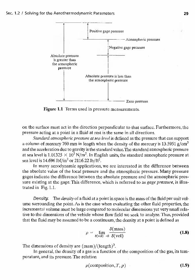
Pressure. Because of the random motion due to their thermal energy, the indi-vidual molecules of a fluid would continually strike a surface that is placed in the fluid.These collisions occur even though the surface is at rest relative to the fluid. By Newton'ssecond law, a force is exerted on the surface equal to the time rate of change of the mo-mentum of the rebounding molecules. Pressure is the magnitude of this force per unitarea of surface. Since a fluid that is at rest cannot sustain tangential forces, the pressure
Sec. 1.2 / Solving for the Aerothermodynamic Parameters 29
Positive gage pressure
Atmospheric pressure
Negative gage pressure
Absolute pressureis greater than
the atmosphericpressure
Absolute pressure is less thanthe atmospheric pressure
Zero pressure
Figure 1.1 Terms used in pressure measurements.
on the surface must act in the direction perpendicular to that surface. Furthermore, thepressure acting at a point in a fluid at rest is the same in all directions.
Standard atmospheric pressure at sea level is defined as the pressure that can supporta column of mercury 760 mm in length when the density of the mercury is 13.595 1 g/cm3and the acceleration due to gravity is the standard value. The standard atmospheric pressureat sea level is 1.01325 x N/rn2. In English units, the standard atmospheric pressure atsea level is 14.696 lbf/in2 or 2116.22 lb/ft2.
In many aerodynamic applications, we are interested in the difference betweenthe absolute value of the local pressure and the atmospheric pressure. Many pressuregages indicate the difference between the absolute pressure and the atmospheric pres-sure existing at the gage. This difference, which is referred to as gage pressure, is illus-trated in Fig. 1.1.
Density. The density of a fluid at a point in space is the mass of the fluid per unit vol-ume surrounding the point. As is the case when evaluating the other fluid properties, theincremental volume must be large compared to molecular dimensions yet very small rela-tive to the dimensions of the vehicle whose flow field we seek to analyze. Thus, providedthat the fluid may be assumed to be a continuum, the density at a point is defined as
8(mass)p lim (1.8)
The dimensions of density are (mass)/(length)3.In general, the density of a gas is a function of the composition of the gas, its tem-
perature, and its pressure. The relation
p(composition, T, p) (1.9)
30 Chap. 1 I Why Study Aerodynamics?
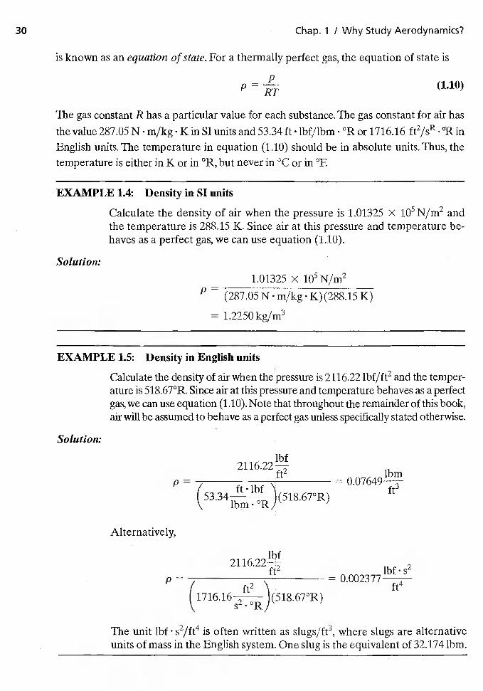
is known as an equation of state. For a thermally perfect gas, the equation of state is
P = (1.10)
The gas constant R has a particular value for each substance. The gas constant for air has
the value 287.05 N rn/kg K in SI units and 53.34 ft lbf/lbm °R or 1716.16 ft2/sR . °R in
English units. The temperature in equation (1.10) should be in absolute units. Thus, thetemperature is either in K or in °R, but never in °C or in °F.
EXAMPLE 14: Density in SI units
Calculate the density of air when the pressure is 1.01325 x i05 N/rn2 andthe temperature is 288.15 K. Since air at this pressure and temperature be-haves as a perfect gas, we can use equation (1.10).
Solution:
1.01325 X N/rn2
(287.05 N rn/kg. K)(288.15 K)
= 1.2250 kg/rn3
EXAMPLE 15: Density in English units
Calculate the density of air when the pressure is 2116.22 lbf/ft2 and the temper-ature is 518.67°R. Since air at this pressure and temperature behaves as a perfectgas, we can use equation (1.10).Note that throughout the remainder of this book,air will be assumed to behave as a perfect gas unless specifically stated otherwise.
Solution:
2116.22—ft2
=ft3
Alternatively,
2116.22— 2ft2 =
/ ft2 \. ft4I 1716.16 I(51867°R)
s2°RJ
The unit lbf s2/ft4 is often written as slugs/ft3, where slugs are alternativeunits of mass in the English systern. One slug is the equivalent of 32.174 Ibm.
Sec. 1.2 / Solving for the Aerothermodynamic Parameters
For vehicles that are flying at approximately 100 mIs (330 ftls), or less, the den-sity of the air flowing past the vehicle is assumed constant when obtaining a solu-tion for the flow field. Rigorous application of equation (1.10) would require thatthe pressure and the temperature remain constant (or change proportionally) inorder for the density to remain constant throughout the flow field. We know that thepressure around the vehicle is not constant, since the aerodynamic forces and mo-ments in which we are interested are the result of pressure variations associatedwith the flow pattern. However, the assumption of constant density for velocitiesbelow 100 rn/s is a valid approximation because the pressure changes that occurfrom one point to another in the flow field are small relative to the absolute valueof the pressure.
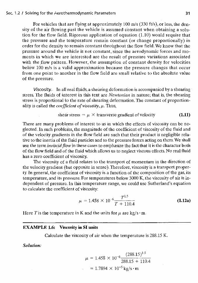
Viscosity.. In all real fluids, a shearing deformation is accompanied by a shearingstress. The fluids of interest in this text are Newtonian in nature; that is, the shearingstress is proportional to the rate of shearing deformation. The constant of proportion-ality is called the coefficient of viscosity, Thus,
shear stress X transverse gradient of velocity (1.11)
There are many problems of interest to us in which the effects of viscosity can be ne-glected. In such problems, the magnitude of the coefficient of viscosity of the fluid andof the velocity gradients in the flow field are such that their product is negligible rela-tive to the inertia of the fluid particles and to the pressure forces acting on them. We shalluse the term inviscid flow in these cases to emphasize the fact that it is the character bothof the flow field and of the fluid which allows us to neglect viscous effects. No real fluidhas a zero coefficient of viscosity.
The viscosity of a fluid relates to the transport of momentum in the direction ofthe velocity gradient (but opposite in sense). Therefore, viscosity is a transport proper-ty. In general, the coefficient of viscosity is a function of the composition of the gas, itstemperature, and its pressure. For temperatures below 3000 K, the viscosity of air is in-dependent of pressure. In this temperature range, we could use Sutherland's equationto calculate the coefficient of viscosity:
= 1.458 x 10⁻⁶T ±110.4
(1.12a)
Here T is the temperature in K and the units for are kg/s m.
EXAMPLE 1.6: Viscosity in SI units
Calculate the viscosity of air when the temperature is 288.15 K.
Solution:
(288.15)i5= 1.458 x 10—6
288.15 + 110.4
= 1.7894 x i05 kg/s m
32 Chap. 11 Why Study Aerodynamics?
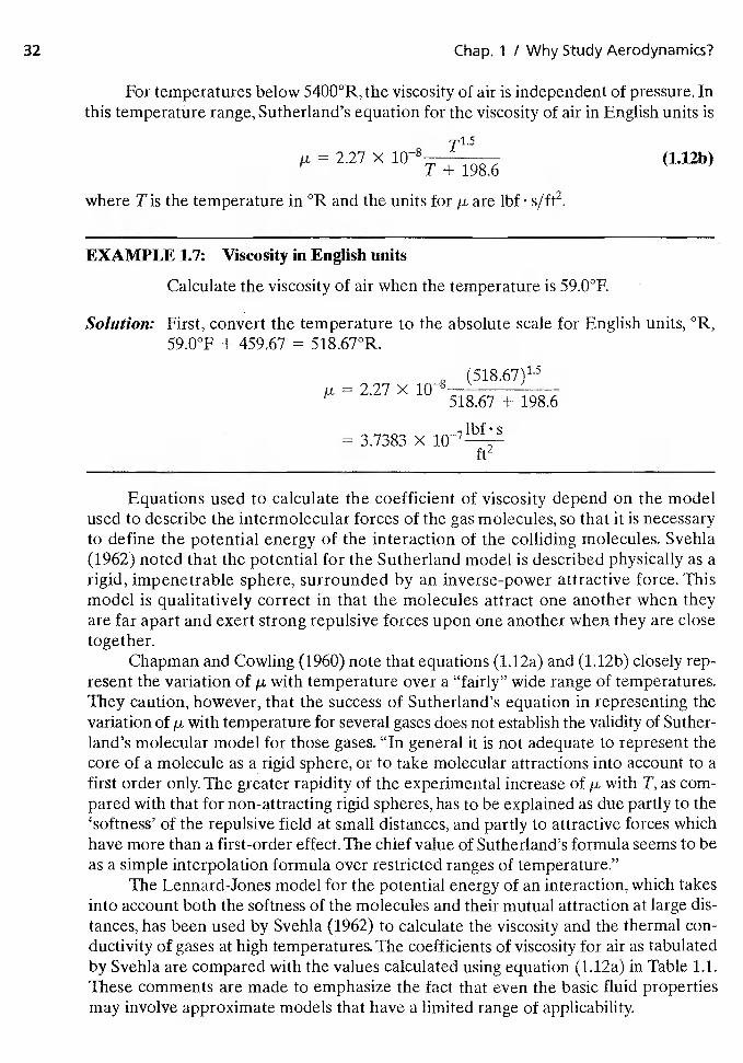
For temperatures below 5400°R, the viscosity of air is independent of pressure. Inthis temperature range, Sutherland's equation for the viscosity of air in English units is
= 2.27 X 10⁸T ±198.6
where T is the temperature in °R and the units for are lbf s/ft2.
EXAMPLE 1.7: Viscosity in English units
Calculate the viscosity of air when the temperature is 59.0°F.
Solution: First, convert the temperature to the absolute scale for English units, °R,59.0°F + 459.67 = 518.67°R.
2.27 x 108518.67 ± 198.6
= 3.7383 x1071bfs
ft2
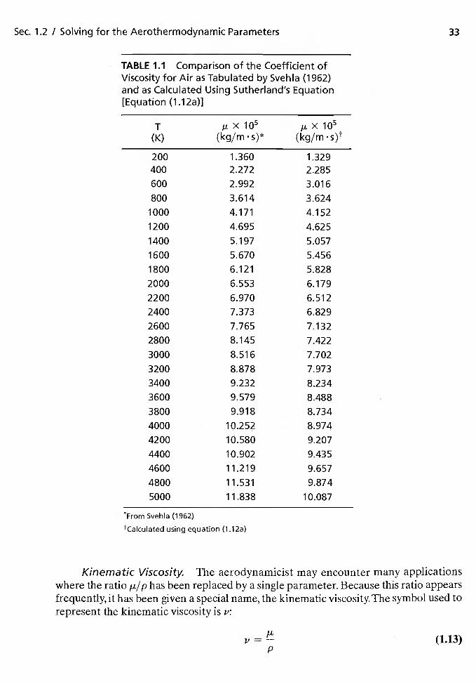
Equations used to calculate the coefficient of viscosity depend on the modelused to describe the intermolecular forces of the gas molecules, so that it is necessaryto define the potential energy of the interaction of the colliding molecules. Svehla(1962) noted that the potential for the Sutherland model is described physically as arigid, impenetrable sphere, surrounded by an inverse-power attractive force. Thismodel is qualitatively correct in that the molecules attract one another when theyare far apart and exert strong repulsive forces upon one another when they are closetogether.
Chapman and Cowling (1960) note that equations (1.12a) and (1.12b) clOsely rep-resent the variation of jt with temperature over a "fairly" wide range of temperatures.They caution, however, that the success of Sutherland's equation in representing thevariation of j.t with temperature for several gases does not establish the validity of Suther-land's molecular model for those gases. "In general it is not adequate to represent thecore of a molecule as a rigid sphere, or to take molecular attractions into account to afirst order only. The greater rapidity of the experimental increase of with T, as com-pared with that for non-attracting rigid spheres, has to be explained as due partly to the'softness' of the repulsive field at small distances, and partly to attractive forces whichhave more than a first-order effect. The chief value of Sutherland's formula seems to beas a simple interpolation formula over restricted ranges of temperature."
The Lennard-Jones model for the potential energy of an interaction, which takesinto account both the softness of the molecules and their mutual attraction at large dis-tances, has been used by Svehla (1962) to calculate the viscosity and the thermal con-ductivity of gases at high temperatures. The coefficients of viscosity for air as tabulatedby Svehla are compared with the values calculated using equation (1.12a) in Table 1.1.These comments are made to emphasize the fact that even the basic fluid propertiesmay involve approximate models that have a limited range of applicability.
Sec. 1.2 I Solving for the Aerothermodynamic Parameters 33
TABLE 1.1 Comparison of the Coefficient ofViscosity for Air as Tabulated by Svehla (1962)and as Calculated Using Sutherland's Equation[Equation (1.12a)]
T(K) (kg/m.s)* (kg/m.s)t
200 1.360 1.329400 2.272 2.285
600 2.992 3.016
800 3.614 3.624
1000 4.171 4.152
1200 4.695 4.625
1400 5.057
1600 5.670 5.456
1800 6.121 5.828
2000 6.553 6.179
2200 6.970 6.512
2400 7.373 6.829
2600 7.765 7.132
2800 8.145 7.422
3000 8.516 7.702
3200 8.878 7.973
3400 9.232 8.234
3600 9.579 8.4883800 9.918 8.734
4000 10.252 8.974
4200 10.580 9.207
4400 10.902 9.435
4600 11.219 9.657
4800 11.531 9.874
5000 11.838 10.087
From Svehla (1962)
tCalculated using equation (1.1 2a)
Kinematic Viscosity. The aerodynamicist may encounter many applicationswhere the ratio p,/p has been replaced by a single parameter. Because this ratio appearsfrequently, it has been given a special name, the kinematic viscosity. The symbol used torepresent the kinematic viscosity is v:
1) = (1.13)p
34 Chap. 1 / Why Study Aerodynamks?
In this ratio, the force units (or. equivalently, the mass units) canceL Thus, v has the dimen-sions of L2/T (e.g., square meters per second or square feet per second).
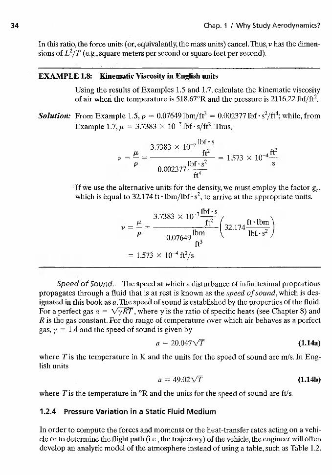
EXAMPLE 1.8: Kinematic Viscosity in English units
Using the results of Examples 1.5 and 1.7, calculate the kinematic viscosityOf air when the temperature is 518.67°R and the pressure is 2116.22 lbf/ft2.
Solution: From Example 1.5, p = 0.07649 lbm/ft3 = 0.002377 lbf s2/ft4; while, fromExample 1.7, p. = 3.7383 X lbf s/ft2. Thus,
3.7383p. = ft2
= 1.573 x 10-p S
0.002377ft4
If we use the alternative units fr the density, we must employ the factorWhich is equal to 32.174 ft lbm/lbf s2, to arrive at the appropriate units.
3.7383 x= p. = ft2 (32. 174ft lbm
pft3
= 1.573 x 104ft2/s
Speed of Sound. The speed at which a disturbance of infinitesimal proportionspropagates through a fluid that is at rest is known as the speed of sound, which is des-ignated in this book as a. The speed of sound is established by the properties of the fluid.For a perfect gas a = where yis the ratio of specific heats (see Chapter 8) andR is the gas constant. For the range Of temperature over which air behaves as a perfectgas, y = 1.4 and the speed of sound is given by
a = 20.047VT (1.14a)
where T is the temperature in K and the units for the speed of sound are rn/s. In Eng-lish units
a 49.02 VT (L14b)
where T is the temperature in °R and the units for the speed of sound are ft/s.
1.2.4 PressUre Variation in a Static Fluid Medium
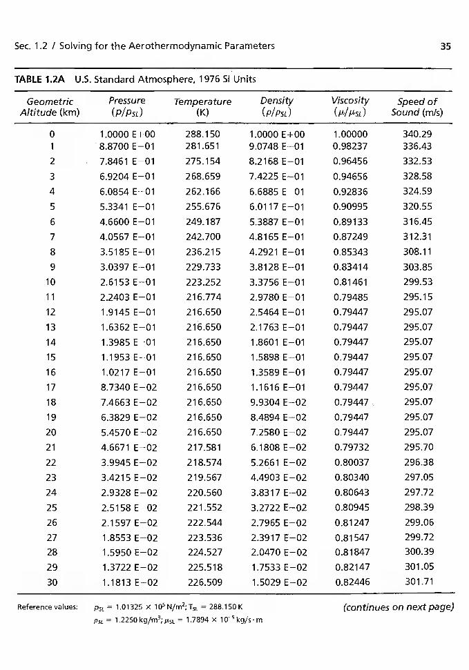
In order to compute the forces and moments or the heat-transfer rates acting on a vehi-cle or to determine the flight path (i.e., the trajectory) of the vehicle, the engineer will oftendevelop an analytic model of the atmosphere instead of using a table,such as Table 1.2.
Sec. 1.2 1 Solving for the Aerothermodynamic Parameters 35
TABLE 1.2A U.S. Standard Atmosphere, 1976 SI Units
GeometricAltitude (km)
Pressure(PIPSL)
Temperature(K)
Density(P/PsL)
Viscosity Speed ofSound (mis)
0 1.0000E+00 288.150 1.0000E+00 1.00000 340.291 '8.8700 E—01 281 .651 9.0748 E—01 0.98237 336.43
2 7.8461 E—O1 275.154 8.2168 E—01 0.96456 332.53
3 6.9204 E—01 268.659 7.4225 E—01 0.94656 328.58
4 6.0854 E—01 262.166 6.6885 E—01 0.92836 324.59
5 5.3341 E—01 255.676 6.0117 E—01 0.90995 320.55
6 4.6600E—01 249.187 5.3887E—01 0.89133 316.45
7 4.0567 E—01 242.700 4.81 65 E—01 0.87249 312.31
8 3.5185 E—'-Ol 236.215 4.2921 E—01 0.85343 308.11
9 3.0397 E—01 229.733 3.8128 E—01 0.83414 303.85
10 2.61 53 E—01 223.252 3.3756 E—01 0.81461 299.53
11 2.2403 E—01 216.774 2.9780 E—01 0.79485 295.15
12 1.9145E—01 216.650 2.5464E—01 0.79447 295.07
13 1.6362 E—01 216.650 2.1763 E—01 0.79447 295.07
14 1.3985 E—01 216.650 1.8601 E—01 0.79447 295.07
15 1.1953 E—01 21 6.650 1.5898 E—01 0.79447 295.07
16 1.0217 E—01 21 6.650 1.3589 E—01 0.79447 295.07
17 8.7340 E—02 21 6.650 1.1616 E—01 0.79447 295.07
18 7.4663 E—02 21 6.650 9.9304 E—02 0.79447 295.07
19 6.3829 E—02 21 6.650 8.4894 E—02 0.79447 295.07
20 5.4570 E—02 216.650 7.2580 E—02 0.79447 295.07
21 4.6671 E—02 217.581 6.1808 E—02 0.79732 295.70
22 3.9945 E—02 218.574 5.2661 E—02 0.80037 296.38
23 3.4215 E—02 219.567 4.4903 E—02 0.80340 297.05
24 2.9328 E—02 220.560 3.8317 E--02 0.80643 297.72
25 2.5158 E—02 221.552 3.2722 E—02 0.80945 298.39
26 2.1597 E—02 222.544 2.7965 E—02 0.81247 299.06
27 1.8553 E—02 223.536 2.3917 E—02 0.81 547 299.72
28 1.5950 E—02 224.527 2.0470 E—02 0.81847 300.39
29 1.3722E—02 225.518 1.7533E—02 0.82147 301.05
30 1.1813E—02 226.509 1.5029E—02 0.82446 301.71
Reference values: = 1.01325 x N/m2;T51 288.150 K (continues on next page)PSL 1.2258 kg/rn3; = 13894 x 1 kg/s. rn
36 Chap. 1 / Why Study Aerodynamics?
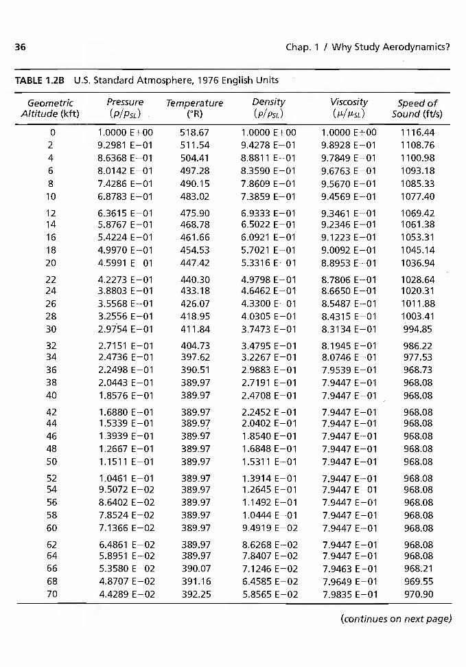
TABLE 1.2B U.S. Standard Atmosphere, 1976 English Units
GeometricAltitude (kft)
Pressure
(P/PSL)Temperature
(°R)
Density(P/PsL)
Viscosity(/1'//l'SL)
Speed ofSound (ft/s)
0 1.0000 E+00 518.67 1.0000 E+OO 1.0000 E+OO 1116.442 9.2981 E—01 511.54 9.4278E—01 9.8928E—01 1108.764 8.6368E—01 504.41 8.8811 E—01 9.7849E—01 1100.986 8.0142 E—01 497.28 8.3590 E—01 9.6763 [—01 1093.188 7.4286 E—01 490.15 7.8609 E—01 9.5670 E—01 1085.3310 6.8783 E—O1 483.02 7.3859 E—O1 9.4569 [—01 1077.40
12 6.3615 E—O1 475.90 6.9333 E—01 9.3461 E—01 1069.4214 5.8767 [—01 468.78 6.5022 E—01 9.2346 E—01 1061.3816 5.4224 [—01 461.66 6.0921 E—01 9.1223 [—01 1053.31
18 4.9970 E—01 454.53 5.7021 E—01 9.0092 [—01 1045.1420 4.5991 E—01 447.42 5.3316 E—01 8.8953 [—01 1036.94
22 4.2273 E—01 440.30 4.9798 E—01 8.7806 E—01 1028.6424 3.8803 [—01 433.18 4.6462 E—01 8.6650 [—01 1020.31
26 3.5568 [—01 426.07 4.3300 E—01 8.5487 E—01 1011.8828 3.2556 E—01 418.95 4.0305 E—01 8.4315 [—01 1003.41
30 2.9754 E—01 411.84 3.7473 E—01 8.3134 E—01 994.85
32 2.7151 [—01 404.73 3.4795 E—01 8.1945 E—01 986.2234 2.4736 E—O1 397.62 3.2267 E—01 8.0746 [—01 977.5336 2.2498 [—01 390.51 2.9883 E—01 7.9539 [—01 968.7338 2.0443 E—01 389.97 2.7191 E—01 7.9447 E—01 968.0840 1.8576 E—01 389.97 2.4708 E—01 7.9447 E—01 968.08
42 1.6880 [—01 389.97 2.2452 E—01 7.9447 [—01 968.0844 1.5339 [—01 389.97 2.0402 E—01 7.9447 [—01 968.0846 1.3939 [—01 389.97 1.8540 E—01 7.9447 [—01 968.0848 1.2667 E—01 389.97 1.6848 E—01 7.9447 E—01 968.0850 1.1511 E—01 389.97 1.5311 E—01 7.9447 E—01 968.08
52 1.0461 E—01 389.97 1.3914 E—01 7.9447 E—01 968.0854 9.5072 E—02 389.97 1.2645 E—01 79447 E—01 968.0856 8.6402 [—02 389.97 1.1492 E—01 7.9447 E—01 968.0858 7.8524 E—02 389.97 1.0444 E—01 7.9447 E—01 968.0860 7.1366 E—02 389.97 9.4919 E—02 7.9447 E—01 968.08
62 6.4861 E—02 389.97 8.6268 E—02 7.9447 E—01 968.0864 5.8951 E—02 389.97 7.8407 E—02 7.9447 [—01 968.0866 5.3580 E—02 390.07 7.1246 E—02 7.9463 E—01 968.21
68 4.8707 [—02 391.16 6.4585 E—02 7.9649 E—01 969.5570 4.4289 E—02 392.25 5.8565 E—02 7.9835 E—01 970.90
(continues on next page)
Sec. 1.2 / Solving for the Aerothermodynamic Parameters 37
TABLE 1.2B U.S. Standard Atmosphere, 1976 English Units (continued)
GeometricAltitude (kft)
Pressure
(P/PSL)Temperature
(CR)
Density(P/PsL)
Viscosity Speed ofSound (ft/s)
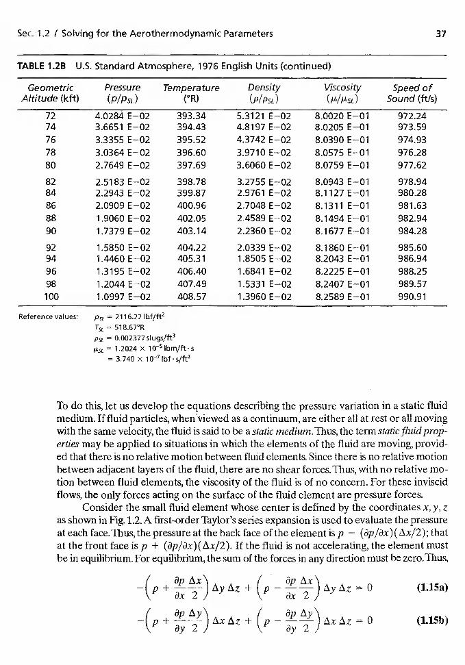
72 4.0284 E—02 393.34 5.3121 E—02 8.0020 E—O1 972.2474 3.6651 E—02 394.43 4.8197 E—02 8.0205 E—01 973.5976 3.3355 E—02 395.52 4.3742 E—02 8.0390 E—01 974.9378 3.0364 E—02 396.60 3.9710 E—02 8.0575 E—01 976.2880 2.7649 E—02 397.69 3.6060 E—02 8.0759 E—01 977.62
82 2.5183 E—02 398.78 3.2755 E—02 8.0943 E—01 978.9484 2.2943 E—02 399.87 2.9761 E—02 8.1127 E—01 980.2886 2.0909E—02 400.96 2.7048E—02 8.1311 E—01 981.6388 1.9060 E—02 402.05 2.4589 E—02 8.1494 E—01 982.9490 1.7379 E—02 403.14 2.2360 E—02 8.1677 E—01 984.28
92 1.5850 E—02 404.22 2.0339 E—02 8.1860 E—01 985.6094 1.4460 E—02 405.31 1.8505 8.2043 E—01 986.9496 1.3195 E-02 406.40 1.6841 E—02 8.2225 E—-01 988.2598 1.2044E—02 407.49 1.5331 E—02 8.2407E—01 989.57100 1.0997 E—02 408.57 1.3960 E—02 8.2589 990.91
Reference values: PSL = 2116.22 tbf/ft2= 518.67°R
PSL = 0.002377 slugs/ft3
= 1.2024 x iCY5= 3.740 X 1 lbf s/ft2
To do this, let us develop the equations describing the pressure variation in a static fluidmedium. If fluid particles, as a continuum, are either all at rest or all movingwith the same velocity, the fluid is said to be a static 1'nediun2.Thus, the term static fluid prop-erties may be applied to situations in which the elements of the fluid are moving, provid-ed that there is no relative motion between fluid elements. Since there is no relative motionbetween adjacent layers of the fluid, there are no shear forces. Thus, with no relative mo-tion between fluid elements, the viscosity of the fluid is of no concern. For these inviscidflows, the only forces acting on the surface of the fluid element are pressure forces.
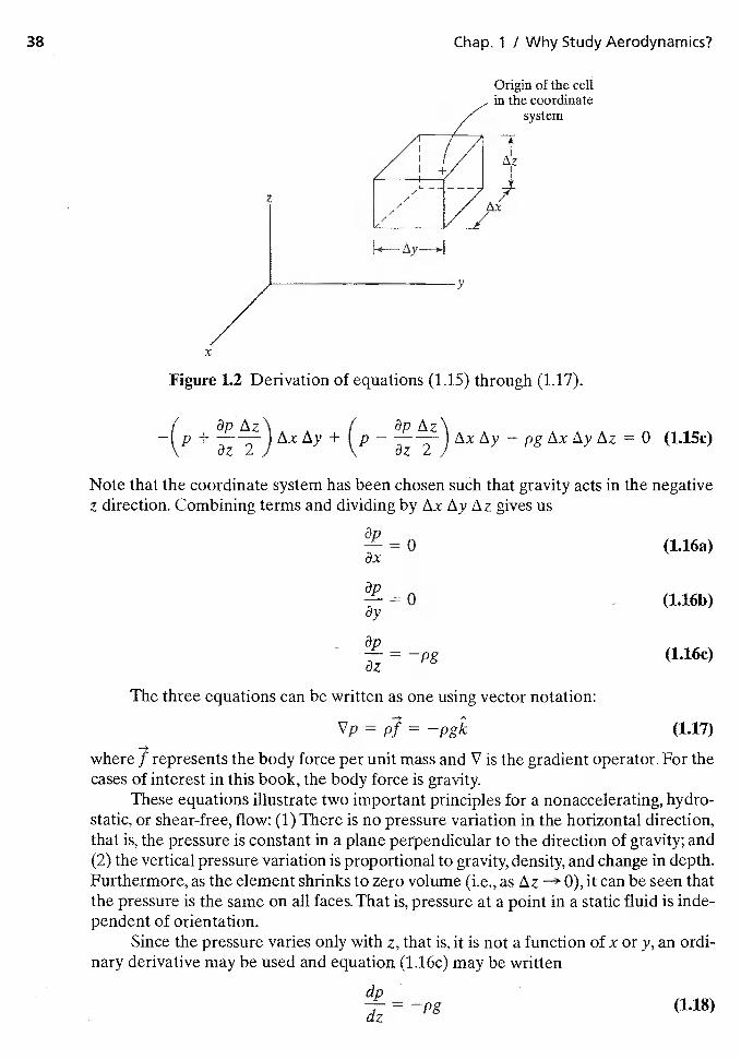
Consider the small fluid element whose center is defined by the coordinates x, y, zas shown in Fig. 1.2. A first-order Taylor's series expansion is used to evaluate the pressureat each face.Thus, the pressure at the back face of the element is p — ( thatat the front face is p + If the fluid is not accelerating, the element mustbe in equilibrium. For equilibrium, the sum of the forces in any direction must be zero. Thus,
I' I 3pLIx\ (LiSa)\ \( ( (L15b)
38 Chap. 1 I WhyStudy Aerodynamics?
z
/Origin of the cellin the coordinate
system
Figure 1,2 Derivation of equations (1.15) through (1.17).
ay
ap
—(p + + (p — — = 0 (1.15c)
Note that the coordinate system has been chosen such that gravity acts in the negativez direction. Combining terms and dividing by txz gives us
(1.16a)
- (1.16b)
(li6c)
The three equations can be written as one using vector notation:
Vp = p7 = —pgk (1.17)
where 7 represents the body force per unit mass and V is the gradient operator. For thecases of interest in this book, the body force is gravity.
These equations illustrate two important principles for a nonaccelerating, hydro-static, or shear-free, flow: (1) There is no pressure variation in the horizontal direction,that is, the pressure is constant in a plane perpendicular to the direction of gravity; and(2) the vertical pressure variation is proportional to gravity, density, and change in depth.Furthermore, as the element shrinks to zero volume (i.e., as —* 0), it can be seen thatthe pressure is the same on all faces. That is, pressure at a point in a static fluid is inde-pendent of orientation.
Since the pressure varies only with z, that is, it is not a function of x or y, an ordi-nary derivative may be used and equation (1.16c) may be written
dp(1.18)
Sec. 1.2 / Solving for the Aerothermôdynamic Parameters 39
Let us assume that the air behaves as a perfect gas. Thus, the expression for den-sity given by equation (1.10) can be substituted into equation (1.18) to give
dp pg= —pg = — (1.19)
In those regions where the temperature can be assumed to constant, separating the vari-ables and integrating between two points yields
fdp P2 g [ gj — = in — = — j dz — — Zi)
where the integration reflects the fact that the temperature has been assumed constant.Rearranging yields
[g(zi — z2)p2piexp[RT
The pressure variation described by equation (1.20) is a reasonable approximation of thatin the atmosphere near the earth's surface.
An improved correlation for pressure variation in the earth's atmosphere can be obtainedif one accounts for the temperature variation with altitude. The earth's mean atmospherictemperature decreases almost linearly with z up to an altitude of nearly 11,000 m.That is,
T=Th-Bzwhere T0 is the sea-level temperature (absolute) and B is the lapse rate, both of which varyfrom day to day.The following standard values will be assumed to apply from 0 to 11,000 m:
T9 = 288.15 K and B = 0.0065 K/rn
Substituting equation (1.21) into the relation
[dp [gdzJp JRT
and integrating, we obtain
/ Bz\g/RBP =
—
(1.22)
The exponent g/RB, which is dimensionless, is equal to 5.26 for air.
1.2.5 The Standard Atmosphere
In order to correlate flight-test data with wind-tunnel data acquired at different timesat different conditions or to compute flow fields, it is important to have agreed-upon stan-dards of atmospheric properties as a function of altitude. Since the earliest days of aero-nautical research, "standard" atmospheres have been developed based on the knowledgeof the atmosphere at thô time. The one used in this text is the 1976 U.S. Standard At-mosphere. The atmospheric properties most commonly used in the analysis and designof ifight vehicles, as taken from the U.S. Standard Atmosphere (1976), are reproducedin Table 1.2. These are the properties used in the examples in this text.
40 Chap. 1 I Why Study Aerodynamics?
The basis for establishing a standard atmosphere is a defined variation of tempera-ture with altitude. This atmospheric temperature profile is developed from measurementsobtained from balloons, from sounding rockets, and from aircraft at a variety of locationsat various times of the year and represents a mean expression of these measurements. Areasonable approximation is that the temperature varies linearly with altitude in some re-gions and is constant in other altitude regions. Given the temperature profile, the hydro-static equation, equation (1.17), and the perfect-gas equation of state, equation (1.10), areused to derive the pressure and the density as functions of altitude. Viscosity and the speedof sound can be determined as functions of altitude from equations such as equation (1.12),Sutherland's equation, and equation (1.14), respectively. In reality, variations would existfrom one location on earth to another and over the seasons at a given location. Never-theless, a standard atmosphere is a valuable tool that provides engineers with a standardwhen conducting analyses and performance comparisons of different aircraft designs.
EXAMPLE 1.9: Properties of the standard ahnosphere at 10 km
Using equations (1.21) and (1.22), calculate the temperature and pressureof air at an altitude of 10 km. Compare the tabulated values with those pre-sented in Table 1.2.
Solution: The ambient temperature at 10,000 mis
T = T0 — Bz = 288.15 — 223.15 K
The tabulated value from Table 1.2 is 223 .252 K.The calculated value for theambient pressure is
I
J 0.0065(104)15.26= 1.01325 x
— 288.15 j= 1.01325 X = 2.641 X N/rn2
The comparable value in Table 1.2 is 2.650 X N/rn2.
EXAMPLE 1.10: Properties of the standard atmosphere in Englishunits
Develop equations for the pressure and for the density as a function of alti-tude from 0 to 65,000 ft.The analytical model of the atmosphere should makeuse of the hydrostatic equations [i.e., equation (1.18)J, for which the densityis eliminated through the use of the equation of state for a thermally perfectgas. Assume that the temperature of air from 0 to 36,100 ft is given by
T = 518.67 — 0.0O3565z
and that the temperature from 36,100 to 65,000 ft is constant at 389.97°R.
Sec. 12 I Solving for the Aerothermodynamic Parameters 41
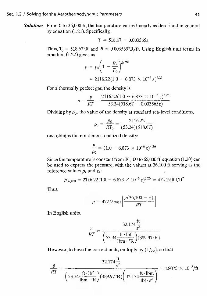
Solution: From 0 to 36,000 ft, the temperature varies linearly as described in generalby equation (1.21). Specifically,
T = 518.67 — 0.003565z
Thus, T0 = 518.67°R and B = 0.003565°R/ft. Using English unit terms inequation (1.22) gives us
I
= 2116.22(1.0 — 6.873 >< z)526
For a thermally perfect gas, the density is
— p — 2116.22(1.0 — 6.873 X z)526
— RT 53.34(518.67 — 0.003S6Sz)
Dividing by p0. the value of the density at standard sea-level conditions,
— — 2116.22Po
RI'0 — (53.34)(518.67)
one obtains the nondimensionalized density:
= (1.0 — 6.873 X 10⁻⁶ z)426Po
Since the temperature is constant from 36,100 to 65,000 ft, equation (1.20) canbe used to express the pressure, with the values at 36,100 ft serving as thereference values Pi and zi:
P36,loo = 2116.22(1.0 6.873 X 10—6 472.19 lbf/ft2
Thus,
Ig(36,100 — z)P=472.9exp[
RI'
In English units,
g s2
RT — ( ft•lbf '\OR)(389.97R)
However, to have the correct units, multiply by (1/ge), so that
32.174g = S = 4.8075 X 10⁵/ft
RT ftlbf /(53.34
lbrn lbf
42 Chap. 1 / Why Study Aerodynamics?
Thus,
= 0.2231 exp (1.7355 — 4.8075 X z)Po
The nondimensionalized density is
p — p T0
p0p0TSince T = 389.97°R = 0.7519T0,
0.2967exp(1.7355 — 4.8075 X 10⁵z)Po
1.3 SUMMARY
Specific values and equations for fluid properties (e.g., viscosity, density, and speed ofsound) have been presented in this chapter. The reader should note that it may be nec-essary to use alternative relations for calculating fluid properties. For instance, for therelatively high temperatures associated with hypersonic flight, it may be necessary to ac-count for real-gas effects (e.g., dissociation). Numerous references present the thermo-dynamic properties and transport properties of gases at high temperatures and pressures[e.g., Moeckel and Weston (1958), Hansen (1957), and Yos (1963)].
PROBLEMS
Problems 1.1 through 1.5 deal with the Energy-Maneuverability Technique for aT-38A thatis powered by two J85-GE-5A enginea Presented in Hg. P1.1 are the thrust available and thethrust required for the T-38A that is cruising at 20,000 feet. The thrust available is presentedas a function of Mach number for the engines operating at military power ("Mit") or oper-ating with the afterburner ("Max"). More will be said about such curves in Chapter 5. Withthe aircraft cruising at a constant altitude (of 20,000 feet), the speed of sound is constant forFig. P1.1 and the Mach number could be replaced by the i.e., by the true air speed.
When the vehicle is cruising at a constant altitude and at a constant attitude, the totaldrag is equal to the thrust required and the lift balances the weight. As will be discussedin Chapter 5, the total drag is the sum of the induced drag, the parasite drag, and thewave drag. Therefore, when the drag (or thrust required) curves are presented for aircraftweights of 8,000 lbf, 10,000 lbf, and 12,000 lbf, they reflect the fact that the induced dragdepends on the lift. But the lift is equal to the weight. Thus, at the lower velocities, wherethe induced drag dominates, the drag is a function of the weight of the aircraft.1.1. The maximum velocity at which an aircraft can cruise occurs when the thrust available with
the engines operating with the afterburner lit ("Max") equals the thrust required, whichare represented by the bucket shaped curves. What is the maximum cruise velocity that alO,000-lbf T-38A can sustain at 20,000 feet?As the vehicle slows down, the drag acting on the vehicle (which is equal to the thrust requiredto cruise at constant velocity and altitude) reaches a minimum (Dmjn). The lift-to-drag ratio
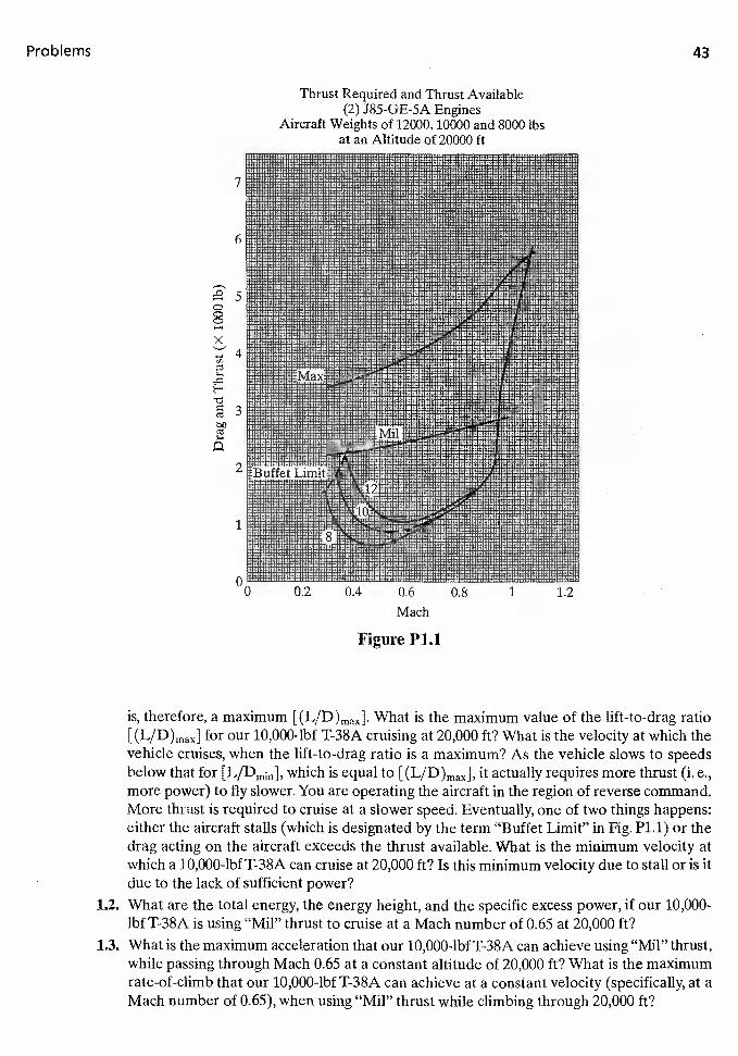
Problems 43
'-'4
><
I-,
C
Thrust Required and Thrust Available(2) J85-GE-5A Engines
Aircraft Weights of 12000, 10000 and 8000 lbsat an Altitude of 20000 ft
is, therefore, a maximum [(LID )max]. What is the maximum value of the lift-to-drag ratio[(L/D)max] for our 10,000-lbf T-38A cruising at 20,000 It? What is the velocity at which thevehicle cruises, when the lift-to-drag ratio is a maximum? As the vehicle slows to speedsbelow that for [L/Dmju], which is equal to [(L/D )max]' it actually requires more thrust (i. e.,more power) to fly slower. You are operating the aircraft in the region of reverse command.More thrust is required to cruise at a slower speed. Eventually, one of two things happens:either the aircraft stalls (which is designated by the term "Buffet Limit" in Fig. P1.1) or thedrag acting on the aircraft exceeds the thrust available. What is the minimum velocity atwhich a 10,000-lbfT-38A can cruise at 20,000 ft? Is this minimum velocity due to stall or is itdue to the lack of sufficient power?
1.2. What are the total energy, the energy height, and the specific excess power, if our 10,000-lbf T-38A is using "Mil" thrust to cruise at a Mach number of 0,65 at 20,000 It?
1.3. What is the maximum acceleration that our 10,000-lbfT-38A can achieve using "Mil" thrust,while passing through Mach 0.65 at a constant altitude of 20,000 It? What is the maximumrate-of-climb that our 10,000-lbfT-38A can achieve at a constant velocity (specifically, at aMach number of 0.65), when using "Mu" thrust while climbing through 20,000 ft?
Mach
Figure P1.1
44 Chap. 1 / Why Study Aerodynamics?
1.4. Compare the values of (L/D)max for aircraft weights of 8,000 lbf, 10,000 Ibf, and 12,000 lbf,when ourT-38A aircraft cruises at 20,000 ft. Compare the velocity that is required to cruiseat (L/D)max for each of the three aircraft weights.
iS. Compare the specific excess power for a 10,000-lbf T-38A cruising at the Mach numberrequired for while operating at "Mit" thrust with that for the aircraft cruising ata Mach number of 0.35 and with that for the aircraft cruising at a Mach number of 0.70.
1.6. Nitrogen is often used in wind tunnels as the test gas substitute for air. Compare the valueof the kinematic viscosity
(1.6)
for nitrogen at a temperature of 350°F and at a pressure of 150 psia with that for air at thesame conditions.
The constants for Sutherland's equation to calculate the coefficient of viscosity, i.e.,Eqn. 1.12b, are:
C1 = 2.27 x and C2 = 198.6°R
for air. Similarly,
C1 2.16 x 10⁻⁸ and C2 = 183.6°R
for nitrogen. The gas constant, which is used in the calculation of the density for a thermallyperfect gas,
(1.10)
ftlbf .
is equal to°R
for air and to 55.15thm• °R
for nitrogen.
1.7. Compare the value of the kinematic viscosity for nitrogen in a wind-tunnel test, where thefree-stream static pressure is 586 N/m2 and the free-stream static temperature is 54.3 K, withthe value for air at the same conditions.
The constants for Sutherland's equation to calculate the coefficient of viscosity, i.e.,Eqn. 1.12a, are:
kgC1 = 1.458 x and C2 = 110.4K
s • K05
f or air. Similarly,
kaC1 1.39 X 10_6 b
and C2 = 102Ks m K°5
for nitrogen. The gas constant, which is used in the calculation of the density for a thermallyperfect gas,
p = (1.10)
Problems 45
is equal to 287.05 for air and to 297 for nitrogen. What would be the advan-
tage(s) of using nitrogen as the test gas instead of air?1.8. A perfect gas undergoes a process whereby the pressure is doubled and its density is de-
creased to three-quarters of its original value. If the initial temperature is 200°F, what is thefinal temperature in in °C?
1.9. The isentropic expansion of perfect helium takes place such that is a constant. If thepressure decreases to one-half of its original value, what happens to the temperature? Ifthe initial temperature is 20° C, what is the final temperature?
1.10. Using the values for the pressure and for the temperature given in Table 1.2, calculate thedensity [equation (1.10)] and the viscosity [equation (1.12a)] at 20 km. Compare the calcu-lated values with those given in Table 1.2. What is the kinematic viscosity at this altitude[equation (1.13)]?
1.11. Using the values for the pressure and for the temperature given in Table 1.2, calculate thedensity [equation (1.10)] and the viscosity [equation (1.12b)] at 35,000 ft. Compare the cal-culated values with those given in Table 1.2. What is the kinematic viscosity at this altitude[equation (1.13)]?
1.12. The conditions in the reservoir (or stagnation chamber) of Tunnel B at the Arnold Engi-neering Development Center (AEDC) are that the pressure (Pti) is 5.723 X 10⁶ N/rn2 andthe temperature (TA) is 750 K. Using the perfect-gas relations, what are the density and theviscosity in the reservoir?
1.13. The air in Tunnel B is expanded through a convergent/divergent nozzle to the test section,where the Mach number is 8, the free-stream static pressure is 586 N/rn2, and the free-stream temperature is 54.3 K. Using the perfect-gas relations, what are the correspondingvalues for the test-section density, viscosity, and velocity? Note that =
1.14. The conditions in the reservoir (Or stagnation chamber) of Aerothermal Tunnel C at theArnold Engineering Development Center (AEDC) are that the pressure (Psi) is 24.5 psiaand the temperature (Ti) is 1660°R. Using the perfect-gas relations, what are the density andthe viscosity in the reservoir?
1.15. The air in Tunnel C accelerates through a convergent/divergent nozzle until the Machnumber is 4 in the test section. The corresponding values for the free-stream pressure andthe free-stream temperature in the test section are 23.25 lbf/ft2 abs. and —65°F, respec-tively. What are the corresponding values for the free-stream density, viscosity, and ve-locity in the test section? Note that = Using the values for the static pressuregiven in Table 1.2, what is the pressure altitude simulated in the wind tunnel by this testcondition?
1.16. The pilot announces that you are flying at a velocity of 470 knots at an altitude of 35,000 ft.What is the velocity of the airplane in km/h? In ft/s?
1.17. Using equations (1.21) and (1.22), calculate the temperature and pressure of the atmos-phere at 7000 m. Compare the tabulated values with those presented in Table 1.2.
1.18. Using an approach similar to that used in Example 1.7, develop metric-unit expres-sions for the pressure, the temperature, and the density of the atmosphere from 11,000to 20,000 m. The temperature is constant and equal to 216.650 K over this range ofaltitude.
1.19. Using the expressions developed in Problem 1.18, what are the pressure, the density, theviscosity, and the speed of sound for the ambient atmospheric air at 18 km? Compare thesevalues with the corresponding values tabulated in Table 1.2.
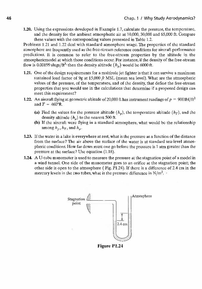
46 Chap. 1 / Why Study Aerodynamics?
1.20. Using the expressions developed in Example 1.7, calculate the pressure, the temperature,and the density for the ambient atmospheric air at 10,000, 30,000 and 65,000 ft. Comparethese values with the corresponding values presented in Table 1.2.
Problems 1.21 and 1.22 deal with standard atmosphere usage. The properties of the standardatmosphere are frequently used as the free-stream reference conditions for aircraft performancepredictions. It is common to refer to the free-stream properties by the altitude in theatmosphericmodel at which those conditions occur. For instance, if the density of the free-streamflow is 0.00199 slugs/It3' then the density altitude (ha) would be 6000 ft.
1.21. One of the design requirements for a multirole jet fighter is that it can survive a maximumsustained load factor of 9g at 15,000 ft MSL (mean sea level). What are the atmosphericvalues of the pressure, of the temperature, and of the density, that define the free-streamproperties that you would use in the calculations that determine if a proposed design canmeet this requirement?
1.22. An aircraft flying at geometric altitude of 20,000 ft has instrument readings of p = 900 lbf/ft2andT = 460°R.
(a) Find the values for the pressure altitude (hr), the temperature altitude (hT), and thedensity altitude (ha) to the nearest 500 ft.
(b) If the aircraft were flying in a standard atmosphere, what would be the relationshipamong hT, and
1.23. If the water in a lake is everywhere at rest, what is the pressure as a function of the distancefrom the surface? The air above the surface of the water is at standard sea-level atmos-pheric conditions. How far down must one go before the pressure is 1 atm greater than thepressure at the surface? Use equation (1.18).
1.24. A U-tube manometer is used to measure the pressure at the stagnation point of a model ina wind tunnel. One side of the manometer goes to an orifice at the stagnation point; theother side is open to the atmosphere (Fig. P1.24). If there is a difference of 2.4 cm in themercury levels in the two tubes, what is the pressure difference in N/rn2.
AtmosphereStagnation
point
Figure P1.24
References 47
1.25. Consult a reference that contains thermodynamic charts for the properties of air, e.g., Hansen(1957), and delineate the temperature and pressure ranges for which air behaves:
p(1) as a thermally perfect gas, i.e., = 1 and
(2) as a calorically perfect gas, i.e., h = cDT, where ci,, is a constant.
1.26. A fairing for an optically perfect window for an airborne telescope is being tested in a windtunnel. A manometer is connected to two pressure ports, one on the inner side of the win-dow and the other port on the outside. The manometer fluid is water. During the testing atthe maximum design airspeed, the column of water in the tube that is connected to the out-side pressure port is 30 cm higher that the column of water in thetube that is connected tothe inside port.(a) What is the difference between the pressure that is acting on the inner surface of the
window relative to the pressure acting on the outer surface of the window?(b) If the window has a total area of 0.5m2, what is the total force acting on the window due
to the pressure difference?
REFERENCES
Chapman S, Cowling TG. 1960. The Mathematical Theory of Non-uniform Gases. Cam-bridge: Cambridge University Press
Coram R. 2002. Boyd, The Fighter Pilot Who Changed the Art of War. Boston: Little Brown
Grier P. 2004. The Viper revolution. Air Force Magazine 87(1):64—69
Hansen CF. 1957. Approximations for the thcrmodynamic properties of air in chemicalequilibrium. NACA Tech. Report R-50
Hillaker H. 1997. Tribute to John R. Boyd. Code One Magazine 12(3)
Moeckel WE, Weston KC. 1958. Composition and thermodynamic properties of air inchemical equilibrium. NACA Tech. Note 4265
Svehla RA.1962. Estimated viscosities and thermal conductivities of gases at high temper-atures. NASA Tech.Report R-132
1976. U. S. Standard Atmospher& Washington, DC: U.S. Government Printing Office
Werner J. 2005. Knight of Germany: Oswald Boelcke — German Ace. Mechanicsburg: Stack-pole Books
Yos 3M. 1963. Transport properties of nitrogen, hydrogen, oxygen, and air to 30,000 K.AVCO Corp. RAD-TM-63-7
2 FUNDAMENTALS OF FLUID
MECHANICS
As noted in Chapter 1, to predict accurately the aerodynamic forces and moments thatact on a vehicle in flight, it is necessary to be able to describe the pattern of flow aroundthe configuration. The resultant flow pattern depends on the geometry of the vehicle, itsorientation with respect to the undisturbed free stream, and the altitude and speed atwhich the vehicle is traveling. The fundamental physical laws used to solve for the fluidmotion in a general problem are
1. Conservation of mass (or the continuity equation)2. Conservation of linear momentum (or Newton's second law of motion)3. Conservation of energy (or the first law of thermodynamics)
Because the flow patterns are often very complex, it may be necessary to use experi-mental investigations as well as theoretical analysis to describe the resultant flow. Thetheoretical descriptions may utilize simplifying approximations in order to obtain anysolution at aH,The validity of the simplifying approximations for a particular applicationshould be verified experimentally. Thus, it is important that we understand the funda-mental laws that govern the fluid motion so that we can relate the theoretical solutionsobtained using approximate flow models with the experimental results, which usually in-volve scale models.
48
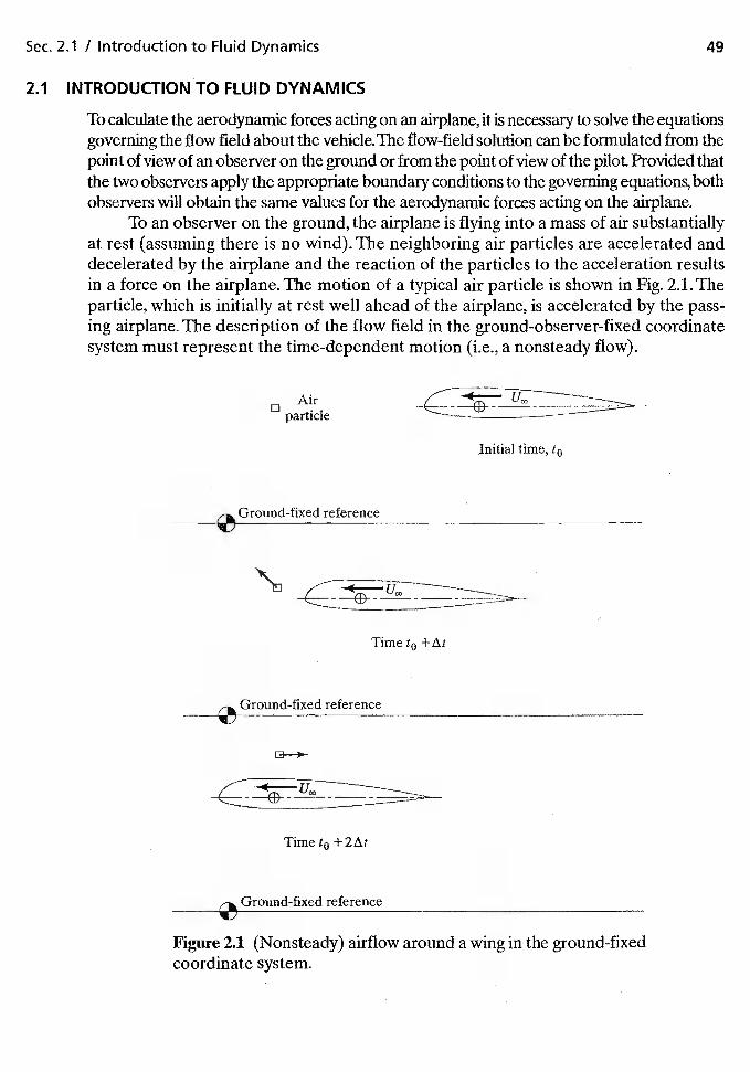
Sec. 2.1 / Introduction to Fluid Dynamics 49
2.1 INTRODUCTION TO FLUID DYNAMICS
To calculate the aerodynamic forces acting on an airplane, it is necessary to solve the equationsgoverning the flow field about the vehicle. The flow-field solution can be formulated from thepoint of view of an observer on the ground or from the point of view of the pilot Provided thatthe two observers apply the appropriate boundary conditions to the governing equations, bothobservers will obtain the same values for the aerodynamic forces acting on the airplane.
To an observer on the ground, the airplane is flying into a mass of air substantiallyat rest (assuming there is no wind). The neighboring air particles are accelerated anddecelerated by the airplane and the reaction of the particles to the acceleration resultsin a force on the airplane. The motion of a typical air particle is shown in Fig. 2.1. Theparticle, which is initially at rest well ahead of the airplane, is accelerated by the pass-ing airplane. The description of the flow field in the ground-observer-fixed coordinatesystem must represent the time-dependent motion (i.e., a nonsteady flow).
°particle
Initial time, t0
Ground-fixed reference
\Time
Ground-fixed reference
Time +2k:
Ground-fixed reference
Figure 2.1 (Nonsteady) airflow around a wing in the ground-fixedcoordinate system.

50 Chap. 2 / Fundamentals of Fluid Mechanics
As viewed by the pilot, the air is flowing past the airplane and moves in response tothe geometry of the vehiclé. If the airplane is flying at constant altitude and constant velocity,the terms of the flow-field equations that contam partial denvatives with respect to timeare zero in the vehicle-fixed coordinate system. Thus, as shown in rig. 2.2, the velocity andthe flow properties of the air particles that pass through a specific location relative to thevehicle are independent of time.The flow field is steady relative to a set of axes fixed to thevehicle (or pilot). Therefore, the equations are usually easier to solve in the vehicle (orpilot)-fixed coordinate system than in the ground-observer-fixed coordinate Becauseof the resulting simplification of the mathematics through Galhlean transformationfrom the grouiid-flxed-reference coordinate system to the vehicle-fixed-reference coordi-nate system, many problems in aerodynamics are formulated as the flow of a stream offluid past a body at rest. Note that the subsequent locations the air particle which passedthrough our control volume at time t0 are mcluded for comparison with Fig 22
In this text we shall use the vehicle (or pilot)-fixed coordinate system. Thus, insteadof descnbmg the fluid motion around a vehicle flying through the air, we will examme air
Vehicle-fixed reference
Initial time, t0
w
)
Controlvolume - Fluid particle which passed
through control volume at time t0
Time t0 +At
w
U.0
ITime t0 +
wFigure 2.2 (Steady) airflow around a wing in a vehicle-fixed coor-dinate system.
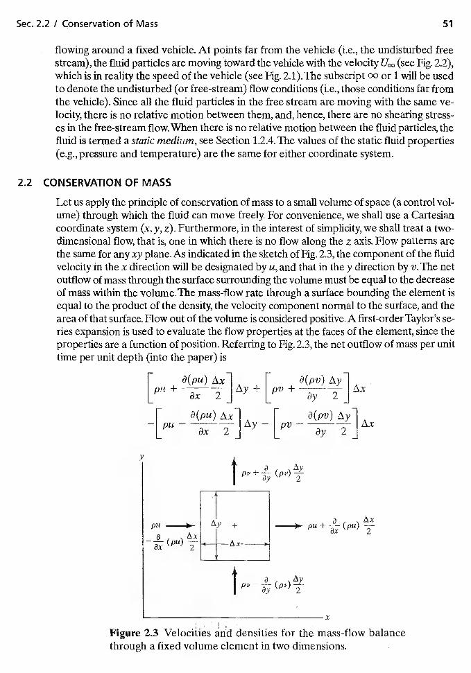
Sec. 2.2 I Conservation of Mass 51
flowing around a fixed vehicle. At points far from the vehicle (i.e., the undisturbed freestream), the fluid particles are moving toward the vehicle with the velocity (see Fig. 2.2),which is in reality the speed of the vehicle (see Fig. 2.1).The subscript 00 or 1 will be usedto denote the undisturbed (or free-stream) flow conditions (i.e., those conditions far fromthe vehicle). Since all the fluid particles in the free stream are moving with the same ve-locity, there is no relative motion between them, and, hence, there are no shearing stress-es in the free-stream flow. When there is no relative motion between the fluid particles, thefluid is termed a static medium, see Section 1.2.4. The values of the static fluid properties(e.g., pressure and temperature) are the same for either coordinate system.
2.2 CONSERVATION OF MASS
Let us apply the principle of conservation of mass to a small volume of space (a control vol..ume) through which the fluid can move freely. For convenience, we shall use a Cartesiancoordinate system (x, y, z). Furthermore, in the interest of simplicity, we shall treat a two-dimensional flow, that is, one in which there is no flow along the z axis. Flow patterns arethe same for any xy plane. As indicated in the sketch of Fig. 2.3, the component of the fluidvelocity in the x direction will be designated by u, and that in the y direction by v. The netoutflow of mass through the surface surrounding the volume must be equal to the decreaseof mass within the volume. The mass-flow rate through a surface bounding the element isequal to the product of the density, the velocity component normal to the surface, and thearea of that surface. Flow out of the volume is considered positive. A first-order Taylor's se-ries expansion is used to evaluate the flow properties at the faces of the element, since theproperties are a function of position. Referring to Fig. 2.3, the net outflow of mass per unittime per unit depth (into the paper) is
[ F r3(pv) zxylpu + + pv +
[ a(pu) F 3(pv)—[Pu
— ax — LPV —
y
PU r
a
x
Figure 2.3 Velociiies and densities for the mass-flow balancethrough a fixed volume element in two dimensions.
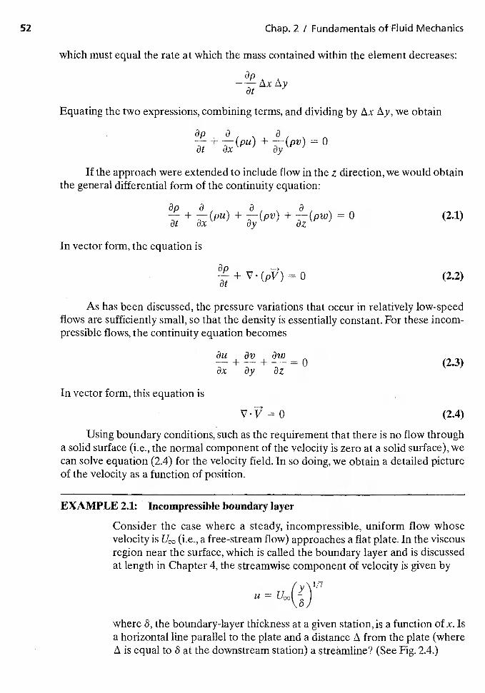
Chap. 2 / Fundament&s of Fluid Mechanics
which must equal the rate at which the mass contained within the element decreases:
— — tXxat
Equating the two expressions, combining terms, and dividing by we obtain
3p a a
lithe approach were extended to include flow in the z direction, we would obtainthe general differential fonn of the continuity equation:
ap a a a+ + + = 0
In vector form, the equation is
+ V (pV) 0 (2.2)
As has been discussed, the pressure variations that occur in relatively low-speedflows are sufficiently small, so that the density is essentially constant. For these incom-pressible flows, the continuity equation becomes
au i3v 8w—+—+-—=O (2.3)ax 8y 8z
In vector form, this equation is
(2.4)
Using boundary conditions, such as the requirement that there is no flow througha solid surface (i.e., the normal component of the velocity is zero at a solid surface), wecan solve equation (2.4) for the velocity field. In so doing, we obtain a detailed pictureof the velocity as a function of position.
EXAMPLE 2.1: Incompressible boundary layer
Consider the case where a steady, incompressible, uniform flow whosevelocity is (i.e., a free-stream flow) approaches a flat plate. In the viscousregion near the surface, which is called the boundary layer and is discussedat length in Chapter 4, the streamwise component of velocity is given by
\ 1/7u =
where 6, the boundary-layer thickness at a given station, is a function of x. Isa horizontal line parallel to the plate and a distance from the plate (where
is equal to 6 at the downstream station) a streamline? (See Fig. 2,4.)
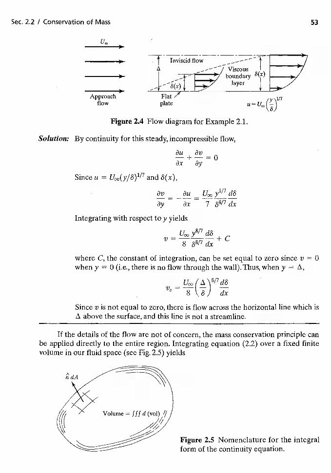
Sec. 2.2 I Conservation of Mass
— 0u —
3y ax — 7
Integrating with respect to y yields
y8"7 d6V = + C
8 dx
where C, the constant of integration, can be set equal to zero since v = 0when y = 0 (i.e., there is no flow through the wall).Thus, when y =
Since v is not equal to zero, there is flow across the horizontal line which isabove the surface, and this line is not a streamline.
If the details of the flow are not of concern, the mass conservation principle canbe applied directly to the entire region. Integrating equation (2.2) over a fixed finitevolume in our fluid space (see Fig. 2.5) yields
Figure 2.5 Nomenclature for the integralform of the continuity equation.
Uco
53
Approachflow (Yplate
Figure 2.4 Flow diagram for Example 2.1.
Solution: By continuity for this steady, incompressible flow,
8u äv—+—=0ax 3y
Since u = and 6(x),
54 Chap. 2 / Fundamentals of Fluid Mechanics
'3p d(vol)+
fff V. (pV)d(vol) = 0
vol VOl
The second volume integral can be transformed into a surface integral using Gauss'stheorem, which is
=
where it dA is a vector normal to the surface dA which is positive when pointing outwardfrom the enclosed volume and which is equal in magnitude to the surface area. The cir-cle through the integral sign for the area indicates that the integration is to be performedover the entire surface bounding the volume. The resultant equation is the general in-tegral expression for the conservation of mass:
+ JpV.itdA = 0 (2.5)
In words, the time rate of change of the mass within the volume plus the net efflux (out-flow) of mass through the surface bounding the volume must be zero.
The volumetric flux Q is the flow rate through a particular surface and is equal toif V•itdA.
For a sample problem using the integral form of the continuity equation, seeExample 2.3.
2.3 CONSERVATION OF LINEAR MOMENTUM
The equation for the conservation of linear momentum is obtained by applying Newton'ssecond law: The net force acting on a fluid particle is equal to the time rate of change ofthe linear momentum of the fluid particle. As the fluid element moves in space, its ve-locity, density, shape, and volume may change, but its mass is conserved. Thus, using a co-ordinate system that is neither accelerating nor rotating, which is called an inertialcoordinate system, we may write
-4
(2.6)
The velocity V of a fluid particle is, in general, an explicit function of time t as well as ofits position x,y, z. Furthermore, the position coordinates x,y, z of the fluid particle arethemselves a function of time. Since the time differentiation of equation (2.6) follows agiven particle in its motion, the derivative is frequently termed the particle, total, orsubstantial derivative of V. Since V(x, y, z, t) and x(t),y(t), and z(t),
dV dx 0V dy aV dz av(2.7)
dt ax dt äy dt az dt at
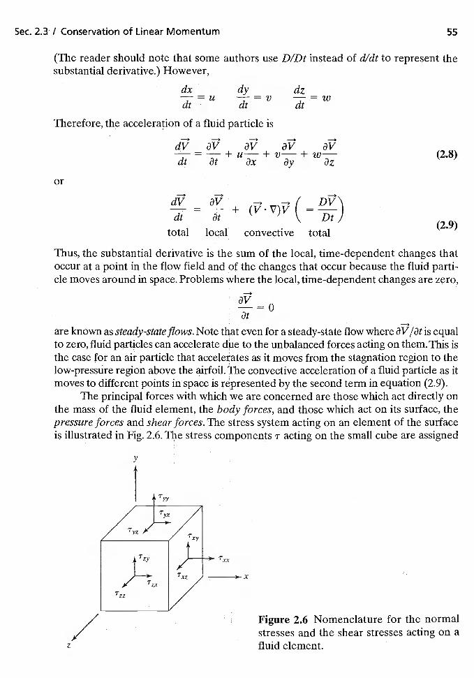
-3 -3 -3dV av au aV aV—=—+u——+v—-+w——dt at ax ay az
dt — at
-3 -* DV
total local convective total
(2.8)
(2.9)
at
Sec. 2.3 I Conservation of Linear Momentum 55
(The reader should note that some authors use D/Dt instead of d/dt to represent thesubstantial derivative.) However,
dx dy dz— = U — = V = Wdt dt dt
Therefore, the acceleration of a fluid particle is
or
Thus, the substantial derivative is the sum of the local, time-dependent changes thatoccur at a point in the flow field and of the changes that occur because the fluid parti-cle moves around in space. Problems where the local, time-dependent changes are zero,
are known as steady-state flows. Note that even for a steady-state flow where ar/at is equalto zero, fluid particles can accelerate due to the unbalanced forces acting on them, This isthe case for an air particle that accelerates as it moves from the stagnation region to thelow-pressure region above the airfoil. The convective acceleration of a fluid particle as itmoves to different points in space is by the second term in equation (2.9).
The principal forces with which we are concerned are those which act directly onthe mass of the fluid element, the body forces, and those which act on its surface, thepressure forces and shear forces. The stress system acting on an element of the surfaceis illustrated in Fig. 2.6. The stress components T acting on the small cube are assigned
Figure 2.6 Nomenclature for the normalstresses and the shear stresses acting on afluid element.
y
/z
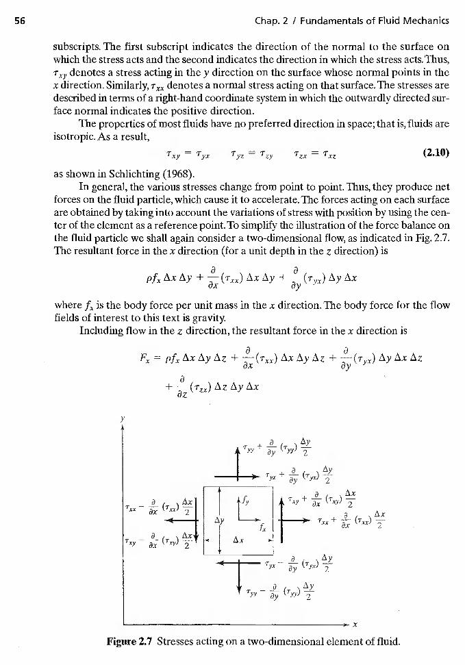
56 Chap. 2 I Fundamentals of Fluid Mechanics
subscripts. The first subscript indicates the direction of the normal to the surface onwhich the stress acts and the second indicates the direction in which the stress acts. Thus,Txy denotes a stress acting in the y direction on the surface whose normal points in thex direction. Similarly, denotes a normal stress acting on that surface. The stresses aredescribed in terms of a right-hand coordinate system in which the outwardly directed sur-face normal indicates the positive direction.
The properties of most fluids have no preferred direction in space; that is, fluids areisotropic. As a result,
'Txy = Tyx Tyz = Tzy Tzx = 'Txz (2.1.0)
as shown in Schlichting (1968).In general, the various stresses change from point to point. Thus, they produce net
forces on the fluid particle, which cause it to accelerate. The forces acting on each surfaceare obtained by taking into account the variations of stress with position by using the cen-ter of the element as a reference point. To simplify the illustration of the force balance onthe fluid particle we shall again consider a two-dimensional flow, as indicated in Fig. 2.7.The resultant force in the x direction (for a unit depth in the z direction) is
+ +
where is the body force per unit mass in the x direction. The body force for the flowfields of interest to this text is gravity.
Including flow in the z direction, the resultant force in the x direction is
+
y
+ (Tyv)
f )i +
a Ax
T_ —+
I Txx +
( — i-.- (Ti)
3'Tyy
Figure 2.7 Stresses acting on a two-dimensional element of fluid.
Sec. 2.3 -I Conservation of Linear Momentum 57
which, by equation (2.6), is equal to
du —+(V.V)u
Equating the two and dividing by the volume of the fluid particle Ax AyAz yields thelinear momentum equation for the x direction:
du a= + + Tyx + Tzx (2.lla)
Similarly, we obtain the equation of motion for the y direction:
dv a a a= + + + (2.1Th)
and for the z direction:
dw a a a= + + Tyz + (2.llc)
Next, we need to relate the stresses to the motion of the fluid. For a fluid at rest or for aflow for which all the fluid particles are moving at the same velocity, there is no shearingstress, and the normal stress is in the nature of a pressure. For fluid particles, the stress isrelated to the rate of strain by a physical law based on the following assumptions:
1. Stress components may be expressed as a linear function of the components ofthe rate of strain. The friction law for the flow of a Newtonian fluid whereT = JL(8u/8y) is a special case of this linear stress/rate-of-strain relation. The vis-cosity /L is more precisely called the first viscosity coefficient. in a more rigorousdevelopment, one should include the second viscosity coefficieni (A), which wouldappear in the normal stress terms. The term involving A disappears completelywhen the flow is incompressible, since V V = 0 by continuity. For other flows,Stokes's hypothesis (A = is presumed to apply See Schlichting (1968).Thesecond viscosity coefficient is of significance in a few specialized problems, such asthe analysis of the shockwave structure, where extremely large changes in pressureand in temperature take place over very short distances.
2. The relations between the stress components and the rate-of-strain componentsmust be invariant to a coordinate transformation consisting of either a rotation ora mirror reflection of axes, since a physical law cannot depend upon the choice ofthe coordinate system.
3. When all velocity gradients are zero (i.e., the shear stress vanishes), the stress com-ponents must reduce to the hydrostatic pressure,p.
For a fluid that satisfies these criteria,
LV +
= —p — +
2 awTzz = — +
3 az
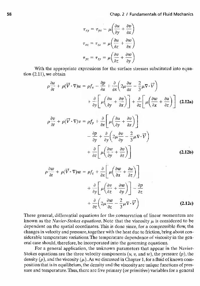
58 Chap. 2 / Fundamentals of Fluid Mechanics
(3u 8v= Tyx +
3W= Tzx = +
/3v 3wTyz = Tzy = +
With the appropriate expressions for the surface stresses substituted into equa-tion (2.11), we obtain
3p 31 3u 2
3 [ (3u 3v\1 3 [ 13w 3u'\1+—l I (2.12a)L \ ay 3x) J i3z [ \ 3x 3z I J
+ p(V V)v + + —
3p 0( äv 2
0y 3y\ äy 3
afl (3w+ —l I (2.12b)
azL \3Y 0z1j
3w ô[f'äw 3u+ p(V V)w +
+
0 [ /Ov Ow\l Op+—lp,(—+—}'——
0YL \Oz Oy)J Oz
3/' Ow 2+ — 2,a— — V ) (2.12c)
OZ\ Oz 3 /These general, differential equations for the conservation of linear momentum areknown as the Navier-Stokes equations. Note that the viscosity is considered to bedependent on the spatial coordinates. This is done since, for a compressible flow, thechanges in velocity and pressure, together with the heat due to friction, bring about con-siderable temperature variations. The temperature dependence of viscosity in the gen-eral case should, therefore, be incorporated into the governing equations.
For a general application, the unknown parameters that appear in the Navier-Stokes equatiOns are the three velocity components (u, v, and w), the pressure (p), thedensity (p), and the viscosity we discussed in Chapter 1, for a fluid of known com-position that is in equilibrium, the density and the viscosity are unique functions of pres-sure and temperature. Thus, there are five primary (or primitive) variables for a general
Sec. 2.4 I Applications to Constant-Property Flows 59
flow problem: the three velocity components, the pressure, and the temperature. How-ever, at present we have only four equations: the continuity equation, equation (2.2), andthe three components of the momentum equation, equations (2.12a) through (2.12c).Tosolve for a general flow involving all five variables, we would need to introduce theenergy equation.
Since equations (2.12a) through (2.12c) are the general differential equations forthe conservation of linear momentum, the equations for a static medium can be obtainedby neglecting the tenns relating to the acceleration of the fluid particles and to the vis-cous forces. Neglecting these terms in equations (2.12a) through (2.12c) and assumingthat the body force is gravity and that it acts in the z direction, the reader would obtainequations (1.16a) through (1.16c).
The integral form of the momentum equation can be obtained by returning toNewton's law. The sum of the forces acting on a system of fluid particles is equal to therate of change of momentum of the fluid particles. Thus, the sum of the body forces andof the surface forces equals the time rate of change of momentum within the volume plusthe net efflux of momentum through the surface bounding the volume. In vector form,
a+ Fsurface = pV d(vol) + J V(pV ii dA) (2.13)
This equation can also be obtained by integrating equation (2.12) over a volume andusing Gauss's Theorem.
2.4 APPUCATIONS TO CONSTANT-PROPERTY FLOWS
For many flows, temperature variations are sufficiently small that the density and vis-cosity may be assumed constant throughout the flow field. Such flows will be termedconstant-property flows in this text. The terms low-speed and/or incompressible flowswill also be used in the description of these flows. A gas flow is considered incompress-ible if the Mach number is less than 0.3 to 0.5, depending upon the application. For theseflows, there are only four unknowns: the three velocity components (u, v, and w), andthe pressure (p). Thus, we have a system of four independent equations that can besolved for the four unknowns; that is, the energy equation is not needed to obtain thevelocity components and the pressure of a constant-property flow.
Let us consider two flows, one for which the solution will beobtained using differential equations and one for which the integral equations are used.
EXAMPLE 2.2: Poiseuille flow
Consider a steady, low-speed flow of a viscous fluid in an infinitely long, two-dimensional channel of height h (Fig. 2.8). This is known as Poiseuille flow.Since the flow is low speed, we will assume that the viscosity and the densityare constant. Because the channel is infinitely long, the velocity componentsdo not change in the x direction. In this text, such a flow is termed a fullydevel aped flow. Let us assume that the body forces are negligible. We are todetermine the velocity profile and the shear-stress distribution.
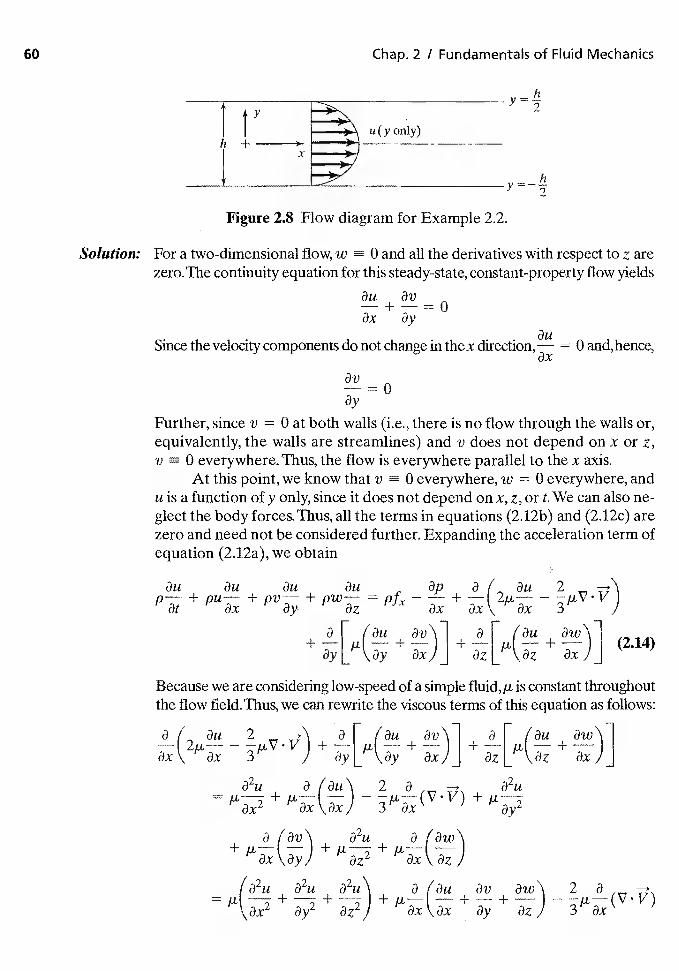
60 Chap. 2 / Fundamentals of Fluid Mechanics
tyI u(yonly)
+
h
Figure 2.8 Flow diagram for Example 2.2.
Solution. For a two-dimensional flow, w 0 and all the derivatives with respect to z arezero.The continuity equation for this steady-state, flow yields
au avax 3y
Smce the velocity components do not change m thex direction, = 0 and, hence,
ay
Further, since v = 0 at both walls (i.e., there is no flow through the walls or,equivalently, the walls are streamlines) and v does not depend on x or z,v 0 everywhere. Thus, the flow is everywhere parallel to the x axis.
At this point, we know that v 0 everywhere, w = 0 everywhere, andu is a function of y only, since it does not depend on x, z, or t. We can also ne-glect the body forces. Thus, all the terms in equations (2.12b) and (2.12c) arezero and need not be considered further. Expanding the acceleration term ofequation (2.12a), we obtain
au au au au ap a I 3u 2
a [ (3u av\1 a r au aw'\1l+—l J.LI—+-—J I (2.14)ay L ay ax)] az L az ax)]
Because we are considering low-speed of a simple is constant throughoutthe flow field. Thus, we can rewrite the viscous terms of this equation as follows:
a / äu 2 —\ a [ lau av'\l a E lau awl+—lpJ—+-—ax 8x 3 1 ay [ \. ay ax!] az [ \. az ax
a2u a /au\ 2 a a2u=+
- +
a a
a2u a a
ay ax
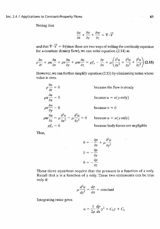
Sec. 2.4/ Applications to Constant-Property Flows
Noting that
3u 8v 8w
3x tOy 8z
and that V V = 0 (since these are two ways of writing the continuity equationfor a constant density flow), we can write equation (2.14) as
tOp (82u 82u 02u\+ + + = — + +
+(2.15)
However, we can further simplify equation (2.15) by eliminating terms whosevalue is zero.
= 0 because the flow is steady
= 0 because a = u(yonly)
= 0 because v 0tOy
t3u 82upw— = = = 0 because u = u(y only)
8x
= 0 because body forces are negligible
Thus,
tOp 82uo = —— + /L—
tOy
tOy
0=——-tOz
These three equations require that the pressure is a function of x only.Recall that a is a function of y only. These two statements can be trueonly if
d2u dp= — = constantdy dx
Integrating twice gives
I dpa = + C1y + C2
aX
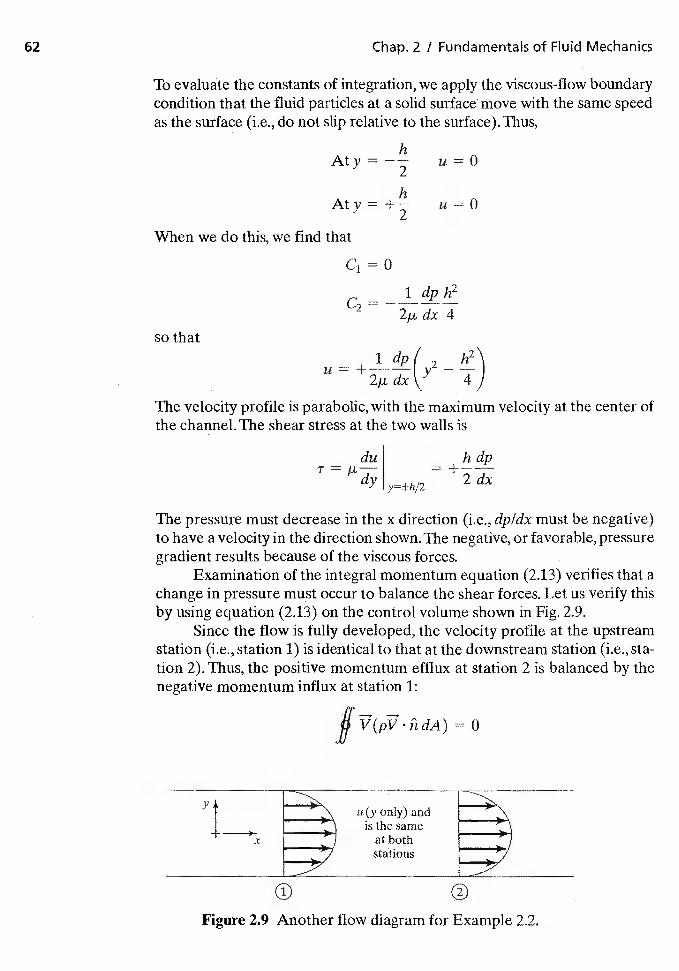
62 Chap. 2 I Fundamentals of Fluid Mechanics
To evaluate the constants of integration, we apply the viscous-flow boundarycondition that the fluid particles at a solid surface move with the same speedas the surface (i.e., do not slip relative to the surface). Thus,
h
u=O
When we do this, we find that
ldph2C2 -
dx 4so that
ldp( h2
2p,dx\\ 4
The velocity profile is parabolic, with the maximum velocity at the center ofthe channel. The shear stress at the two walls is
dudy y=±h/2
The pressure must decrease in the x direction (i.e., dp/dx must be negative)to have a velocity in the direction shown. The negative, or favorable, pressuregradient results because of the viscous forces.
Examination of the integral momentum equation (2.13) verifies that achange in pressure must occur to balance the shear forces. Let us verify thisby using equation (2.13) on the control volume shown in Fig. 2.9.
Since the flow is fully developed, the velocity profile at the upstreamstation (i.e., station 1) is identical to that at the downstream station (i.e., sta-tion 2). Thus, the positive momentum efflux at station 2 is balanced by thenegative momentum influx at station 1:
if =
h dp
©Figure 2.9 Another flow diagram for Example 2.2.
Sec. 2.4 / Applicatiohs to Constant-Property Flows 63
Thus, for this steady flow with negligible body forces,
= 0
or
where the factor of 2 accounts for the existence of shear forces at the upper andlower walls. Finally, as shown in the approach using the differential equation,
p2—p1h dphT-Note, as discussed previously, that there are subtle implications regardingthe signs in these terms. For the velocity profile shown, the shear acts toretard the. fluid motion and the pressure must decrease in the x direction(i.e., dp/dx < 0).
EXAMPLE 2i: Drag on a airfoil
A steady, (V 1L01), low-speed flow approaches a very thin, flat-plate "airfoil" whose length is c. Because of viscosity, the flow near the plateslows, such that velocity measurements at the trailing edge of the plate indi-cate that the x component of the velocity (above the plate) varies as
(y\1/7U —
Below the plate, the velocity is a mirror image of this profile. The pressure is uni-form over the entire cOntrol surface. Neglecting the body forces, what is the dragcoefficient fOr this flow if <3 The drag coefficient is the drag per unitspan (unit depth into the page) divided by the free-stream dynamic pressure
times the reference area per unit span (which is the chord length c):
dCd=
Solution: Let us apply the integral form of the momentum equation [i.e., euation(2.13)] to this flow; Noting that the momentum equation is a vector equation,let us cOnsider thex component only, since that is the direction in which thedrag force acts. Furthermore, since the flow is planar symmetric, only the con-trol volume the plate will be considered (i.e., from y 0 to y = 3).Since the pressure is uniform over the control surface and since the bodyforces are negligible, the only force acting on the fluid in the control volumeis the retarding fOrce of the plate on the fluid, which is —d/2.
Because the flow is steady, the first term on the right-hand side ofequation (2.13) is zero. Thus,
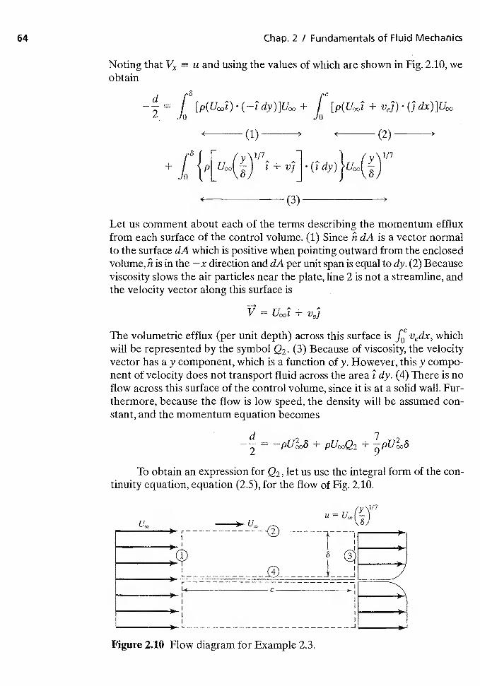
64 Chap. 2 / Fundamentals of Fluid Mechanics
Noting that u and using the values of which are shown in Fig. 2.10, weobtain
d
= J + J +2
(1) (2)
r 1/7 1 ) 1/7
+ I(3)
Let us comment about each of the terms describing the momentum effluxfrom each surface of the control volume. (1) Since dA is a vector normalto the surface dA which is positive when pointing outward from the enclosedvolume, ii is in the —x direction and dA per unit span is equal to dy. (2) Becauseviscosity slows the air particles near the plate, line 2 is not a streamline, andthe velocity vector along this surface is
The volumetric efflux (per unit depth) across this surface is VedX, whichwill be represented by the symbol Q2. (3) Because of viscosity, the velocityvector has a y component, which is a function of y. However, this y compo-nent of velocity does not transport fluid across the area I dy. (4) There is noflow across this surface of the control volume, since it is at a solid wall. Fur-thermore, because the flow is low speed, the density will be assumed con-stant, and the momentum equation becomes
= + +
To obtain an expression for let us use the integral form of the con-tinuity equation, equation (2.5), for the flow of Fig. 2.10.
(y \117
IL0
F
Figure 2.10 Flow diagram for Example 2.3.
Sec. 2.5 / Reynolds Number and Mach Number as Similarity Parameters 65
a
= f+ + fa
+ vJ}(Idy)} =
+ p f VedX + 0 Q2
Substituting this expression into the momentum equation yields
d2
1 2 7d = -
d (0.Olc)Cd = = = 0.00389
1 1 Ti2
2.5 REYNOLDS NUMBER AND MACH NUMBER ASSIMILARITY PARAMETERS
Because of the difficulty of obtaining theoretical solutions of the flow field around avehicle, numerous experimental programs have been conducted to measure directly theparameters that define the flow field. Some of the objectives of such test programs areas follows:
1. To obtain information necessary to develop a flow model that could be used innumerical solutions
2. To investigate the effect of various geometric parameters on the flow field (suchas determining the best location for the engines on a supersonic transport)
3. To verify numerical predictions of the aerodynamic characteristics for a particularconfiguration
4. To measure directly the aerodynamic characteristics of a complete vehicle
Usually, either scale models of the complete vehicle or large-scale simulations ofelements of the vehicle (such as the wing section) have been used in these wind-tunnelprograms. Furthermore, in many test programs, the free-stream conditions (such as thevelocity, the static pressure, etc.) for the wind-tunnel tests were not equal to the valuesfor the flight condition that was to be simulated.
It is important, then, to determine under what conditions the experimental resultsobtained for one flow are applicable toanother flow which is confined by boundaries
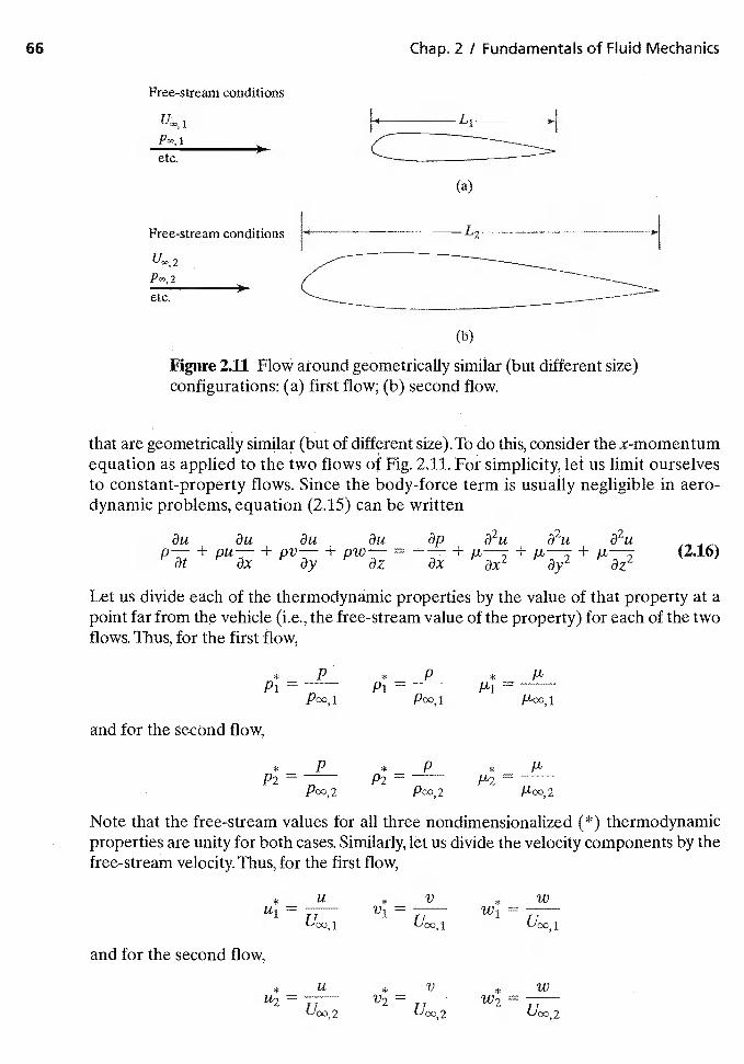
66 Chap. 2 / Fundamentals of Fluid Mechanics
Free-stream conditions
L1
(a)
Free-stream conditions
(ti)
Figure 2.11 Flow around geometrically similar (but different size)configurations: (a) first flow; (b) second flow.
that are geometrically similar (but of different size).To do this, consider the x-momentumequation as applied to the two flows of Fig. 2.11. For simplicity, let us limit ourselvesto constant-property flows. Since the body-force term is usually negligible in aero-dynamic problems, equation (2.15) can be written
8u 8u 3p a2u a2u a2u(2.16)
az ax ax2 3y2 az2
Let us divide each of the thermodynamic properties by the value of that property at apoint far from the vehicle (i.e., the free-stream value of the property) for each of the twoflows. Thus, for the first flow,
* P * P * /1.
Pco,i JLoo 1
and for the second flow,
* P * P */i2—Poo,2 Poo,2
Note that the free-stream values for all three nondimensionalized (*) thermodynamicproperties are unity for both cases. Similarly, let us divide the velocity components by thefree-stream velocity. Thus, for the first flow,
* U * V * wU1= V1= w1=
U00,1 U001
and for the second flow,
* U * V * wU2= V2= w2=
U00,2 U00,2
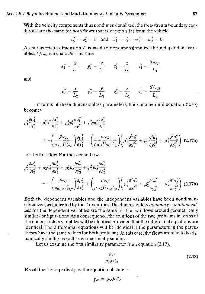
Sec. 2.5 / Reynolds Number and Mach Number as Similarfty Parameters 67
With the velocity components thus nondimensionalized, the free-stream boundary con-ditions are the same for both flows: that is, at points far from the vehicle
and
A characteristic dimension L is used to nondimensionalize the independent vari-ables. L/UOO is a characteristic time.
* x * y * z *tU00,1
x y z *tU03,2
= Y2 = L2 = L2
In terms of these dimensionless parameters, the x-momentum equation (2.16)becomes
* * * ** * *+ + +
at1 3x1 8Yi az1
I POO,i I '\( *2 1* + t J( + p1—7 + (2.17a)
\pooiU00iJ8xi \poo,iUoo,iLiJ\ ax1 3y1 3z1 I
for the first flow. For the second flow,
* *+ + +at2 ax2 ay2 az2
( P00,2\\
ap, ( '\(2 I
Both the dependent variables and the independent variables have been nondimen-sionalized, as indicated by the * quantities. The dimensionless boundary-condition val-ues for the dependent variables are the same for the two flows around geometricallysimilar configurations. As a consequence, the solutions of the two problems in terms ofthe dimensionless variables will be identical provided that the differential equations areidentical. The differential equations will be identical if the parameters in the paren-theses have the same values for both problems. In this case, the flows are said to be dy-namically similar as well as geometrically similar.
Let us examine the first similarity parameter from equation (2.17),
(2.18)p00U00
Recall that for a perfect gas, the equation of state is
p00 p00RT00
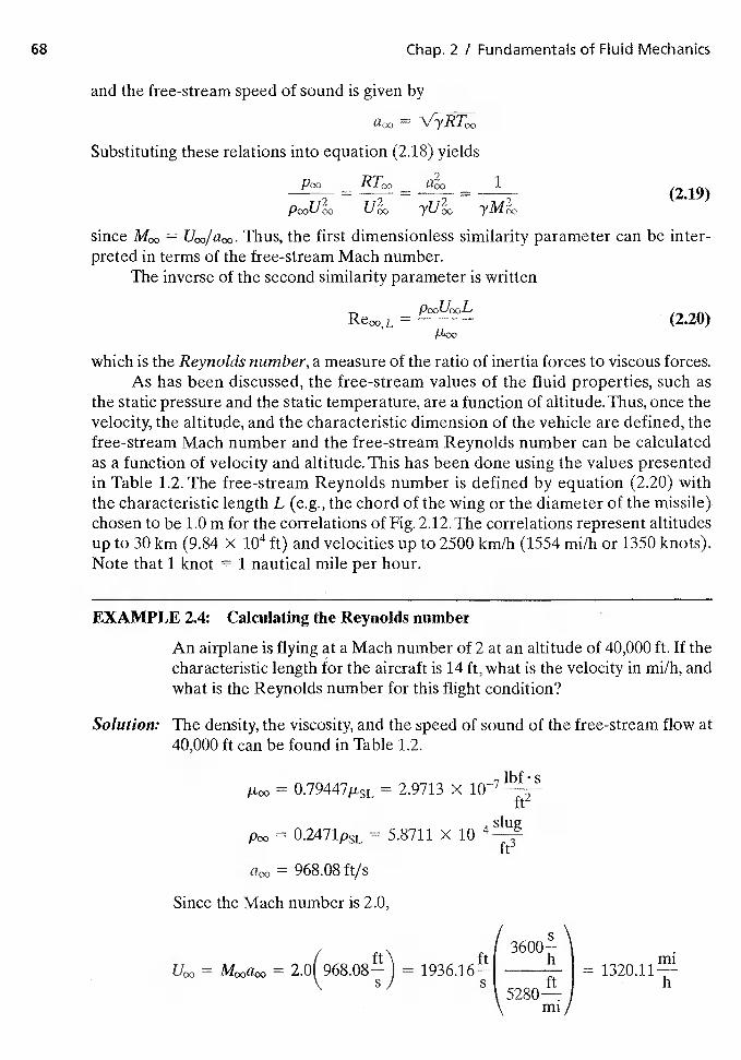
68 Chap. 2 I Fundamentals of Fluid Mechanics
and the free-stream speed of sound is given by
=
Substituting these relations into equation (2.18) yields
1
since = Thus, the first dimensionless similarity parameter can be inter-preted in terms of the free-stream Mach number.
The inverse of the second similarity parameter is written
L
=(2.20)
which is the Reynolds number, a measure of the ratio of inertia forces to viscous forces.As has been discussed, the free-stream values of the fluid properties, such as
the static pressure and the static temperature, are a function of altitude.Thus, once thevelocity, the altitude, and the characteristic dimension of the vehicle are defined, thefree-stream Mach number and the free-stream Reynolds number can be calculatedas a function of velocity and altitude. This has been done using the values presentedin Table 1.2. The free-stream Reynolds number is defined by equation (2.20) withthe characteristic length L (e.g., the chord of the wing or the diameter of the missile)chosen to be 1.0 m for the correlations of Fig. 2,12.The correlations represent altitudesup to 30km (9.84 X i04 ft) and velocities up to 2500 km/h (1554 mi/h or 1350 knots).Note that 1 knot 1 nautical mile per hour.
EXAMPLE Calculating the Reynolds number
An airplane is flying at a Mach number of 2 at an altitude of 40,000 ft. If thecharacteristic length for the aircraft is 14 ft, what is the velocity in mi/h, andwhat is the Reynolds number for this flight condition?
Solution: The density, the viscosity, and the speed of sound of the free-stream flow at40,000 ft can be found in Table 1.2.
= = 2.9713 x
= °.2471PsL = 5.8711 ><
= 968.08 ft/s
Since the Mach number is 2.0,
3600-p-
= =h
=S
5280-p-h
mi
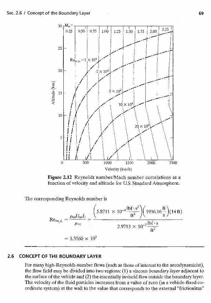
Sec. 2.6 1 Concept of the Boundary Layer
I
Figure 2.12 Reynolds number/Mach number correlations as afunction of velocity and altitude for U.S. Standard Atmosphere.
The corresponding Reynolds number is
69
/-too
lbf.s2\/(5.8711 x iO-4
ft4
2.9713 xft2
= 5.3560 x i07
2.6 CONCEPT OF THE BOUNDARY LAYER
For many high-Reynolds-number flows (such as those of interest to the aerodynamicist),the flow field may be divided into two regions: (1) a viscous boundary layer adjacent tothe surface of the vehicle and (2) the essentially inviscid flow outside the boundary layer.The velocity of the fluid particles increases from a value of zero (in a vehicle-fixed co-ordinate system) at the wall to the value that corresponds to the external "frictionless"
Velocity (kmlh)
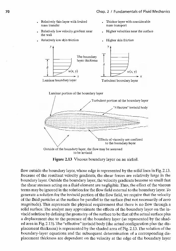
Chap. 2 / Fundamentals of Fluid Mechanics
• Relatively thin layer with limitedmass transfer
• Relatively low velocity gradient nearthe wall
Relatively low skin friction
The boundarylayer thickness
x
• Thicker layer with considerablemass transport
• Higher velocities near the surface
Higher skin friction
Turbulent boundary layerx
Laminar portion of the boundary layer
Outside of the boundary layer, the flow may be assumedto be inviscid
Figure 2.13 Viscous boundary layer on an airfoil.
flow outside the boundary layer, whose edge is represented by the solid lines in Fig. 2.13.Because of the resultant velocity gradients, the shear forces are relatively large in theboundary layer. Outside the boundary layer, the velocity gradients become so small thatthe shear stresses acting on a fluid element are negligible. Thus, the effect of the viscousterms may be ignored in the solution for the flow field external to the boundary layer. Togenerate a solution for the inviscid portion of the flow field, we require that the velocityof the fluid particles at the surface be parallel to the surface (but not necessarily of zeromagnitude). This represents the physical requirement that there is no flow through asolid surface. The analyst may approximate the effects of the boundary layer on the in-viscid solution by defining the geometry of the surface to be that of the actual surface plusa displacement due to the presence of the boundary layer (as represented by the shad-ed area in Fig. 2.13).The "effective" inviscid body (the actual configuration plus the dis-placement thickness) is represented by the shaded area of Fig. 2.13. The solution of theboundary-layer equations and the subsequent determination of a corresponding dis-placement thickness are dependent on the velocity at the edge of the boundary layer
y y
ILaminar boundary layer
Turbulent portion of the boundary layer
"Effective" inviscid body
'Effects of viscosity are confinedto the boundary layer
Sec. 2.6 / Concept of the Boundary Layer 71
(which is, in effect, the velocity at the surface that corresponds to the inviscid solution).The process of determining the interaction of the solutions provided by the inviscid-f lowequations with those for the boundary-layer equations requires a thorough understand-ing of the problem [e.g., refer to Brune et aL, (1974)j.
For many problems involving flow past streamlined shapes such as airfoils andwings (at low angles of attack), the presence of the boundary layer causes the actualpressure distribution to be only negligibly different from the inviscid pressure distribu-tion. Let us consider this statement further by studying the x andy components of equa-tions (2.12) for a two-dimensional incompressible flow. The resultant equations, whichdefine the flow in the boundary layer shown in Fig. 2.13, are
3u 9u au 32u
3x äy 0x 3x2 3y2
and
32v
at ax ay ay ax2 ay2
where the x coordinate is measured parallel to the airfoil surface and the y coordinateis measured perpendicular to it. Solving for the pressure gradients gives us
ä1D ( a a a— — + Pu - + pv - - —i - 1a
aplaProviding that the boundary layer near the solid surface is thin, the normal componentof velocity is usually much less than the streamwise component of velocity (i.e., v < u).Thus, the terms on the right-hand side of the equation in the second line are typicallysmaller than the term in the first line. We conclude, then, that
As a result, the pressure gradient normal to the surface is negligible:
3y
which is verified by experiment. Since the static pressure variation across the boundarylayer is usually negligible, the pressure distribution around the airfoil is essentially thatof the inviscid flow (accounting for the displacement effect of the boundary layer).
The assumption that the static pressure variation across the boundary layer is negli-gible breaks down for turbulent boundary layers at very high Mach numbers. Bushnell et aL,(1977) cite data for which the wail pressure is significantly greater than the edge value forturbulent boundary layers where the edge Mach number is approximately 20. The charac-teristics distinguishing laminar and turbulent boundary layers are discussed in Chapter 4.
72 Chap. 2 / Fundamentals of Fluid Mechanics
When the combined action of an adverse pressure gradient and the viscous forcescauses the boundary layer to separate from the vehicle surface (which may occur forblunt bodies or for streamlined shapes at high angles of attack), the flow field is very sen-sitive to the Reynolds number. The Reynolds number, therefore, also serves as an indi-cator of how much of the flow can be accurately described by the inviscid-flow equations.For detailed discussions of the viscous portion of the flow field, the reader is referred toChapter 4 and to Schlichting (1979), White (2005), Schetz (1993), and Wilcox (1998).
2.7 CONSERVATION OF ENERGY
There are many flows that involve sufficient temperature variations so that convective heattransfer is important, but for which the constant-property assumption is reasonable. An ex-ample is flow in a heat exchanger. For such flows, the temperature field is obtained by solv-ing the energy equation after the velocity field has been determined by solving the continuityequation and the momentum equation. This is because, for this case, the continuity equationand the momentum equation are independent of the energy equation, but not vice versa.
We must also include the energy equation in the solution algorithm for com-pressible flows. Compressible flows are those in which the pressure and temperaturevariations are sufficiently large that we must account for changes in the other fluid prop-erties (e.g., density and viscosity). For compressible flows, the continuity equation, themomentum equation, and the energy equation must be solved simultaneously. Recall thediscussion relating to equations (2.12a) through (2.12c).
In the remainder of this chapter, we derive the energy equation and discuss its ap-plication to various flows.
2.8 FIRST LAW OF THERMODYNAMICS
Consider a system of fluid particles. Everything outside the group of particles is calledthe surroundings of the system. The first law of thermodynamics results from the fun-damental experiments of James Joule. Joule found that, for a cyclic process, that is, onein which the initial state and the final state of the fluid are identical,
— = 0 (2.21)
Thus, Joule has shown that the heat transferred from the surroundings to the systemless the work done by the system on its surroundings during a cyclic process is zero.In equation (2.21), we have adopted the convention that heat transfer to the systemis positive and that work done by the system is positive. The use of lower case symbolsto represent the parameters means that we are considering the magnitude of the pa-rameter per unit mass of the fluid. We use the symbols 8q and &w to designate that theincremental heat transfer to the system and the work done by the system are not exactdifferentials but depend on the process used in going from state 1 to state 2. Equation(2.21) is true for any and all cyclic processes. Thus, if we apply it to a process that takesplace between any two states (1 and 2), then
— 6w = de e2 — e1 (2.22)
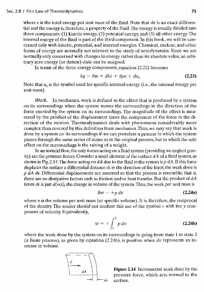
Sec. 2.8 I First Law of Thermodynamics 73
where e is the total energy per unit mass of the fluid. Note that de is an exact differen-tial and the energy is, therefore, a property of the fluid. The energy is usually divided intothree components: (1) kinetic energy, (2) potential energy, and (3) all other energy. Theinternal energy of the fluid is part of the third component. In this book, we will be con-cerned only with kinetic, potential, and internal energies. Chemical, nuclear, and otherforms of energy are normally not relevant to the study of aerodynamics. Since we arenormally only concerned with changes in energy rather than its absolute value, an arbi-trary zero energy (or datum) state can be assigned.
In terms of the three energy components, equation (2.22) becomes
6q — dke + dpe + dUe (2.23)
Note that Ue is the symbol used for specific internal energy (i.e., the internal energy perunit mass).
Work. In mechanics, work is defined as the effect that is produced by a systemon its surroundings when the system moves the surroundings in the direction of theforce exerted by the system on its surroundings. The magnitude of the effect is mea-sured by the product of the displacement times the component of the force in the di-rection of the motion. Thermodynamics deals with phenomena considerably morecomplex than covered by this definition from mechanics. Thus, we may say that work isdone by a system on its surroundings if we can postulate a process in which the systempasses through the same series of states as in the original process, but in which the soleeffect on the surroundings is the raising of a weight.
In an inviscid flow, the only forces acting on a fluid system (providing we neglect grav-ity) are the pressure forces. Consider a small element of the surface dA of a fluid system, asshown in Fig. 2.14. The force acting on dA due to the fluid in the system isp dA. If this forcedisplaces the surface a differential distance dg in the direction of the force, the work done isp dA ds. Differential displacements are assumed so that the process is reversible; that is,there are no dissipative factors such as friction and/or heat transfer. But the product of dAtimes is just d(vol), the change in volume of the system. Thus, the work per unit mass is
= +p dv (2.24a)
where v is the volume per unit mass (or specific volume). It is, therefore, the reciprocalof the density. The reader should not confuse this use of the symbol v with the y com-ponent of velocity. Equivalently,
w =+ j.2
p dv (2.24b)
where the work done by the system on its surroundings in going from state 1 to state 2(a finite process), as given by equation (2.24b), is positive when dv represents an in-crease in volume.
Figure 2.14 Incremental work done by thepressure force, which acts normal to thesurface.
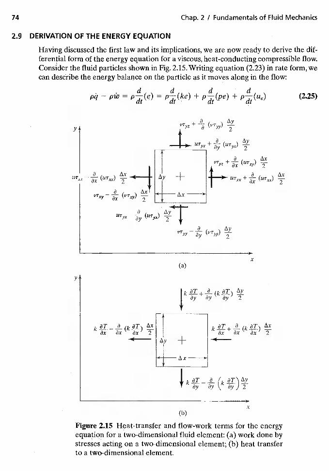
74 Chap. 2 I Fundamentals of Fluid Mechanics
2.9 DERIVATION OF THE ENERGY EQUATION
Having discussed the first law and its implications, we are now ready to derive the dif-ferential foñn of the energy equation for a viscous, heat-conducting compressible flow.Consider the fluid particles shown in Fig. 2.15. Writing equation (2.23) in rate form, wecan describe the energy balance on the particle as it moves ajong in the flow:
d d dpq — pw = = + +
V ay)T
(b)
Figure 2.15 Heat-transfer and flow-work terms for the energyequation for a two-dimensional fluid element: (a) work done bystresses acting on a two-dimensional element; (b) heat transferto a two-dimensional element.
(2.25)
2
a+ -b---- T
avrxy —
2
y
—.
y
a+ T
a—
2
(a)x
ax ax ax 2 ax ax ax 24y+
x
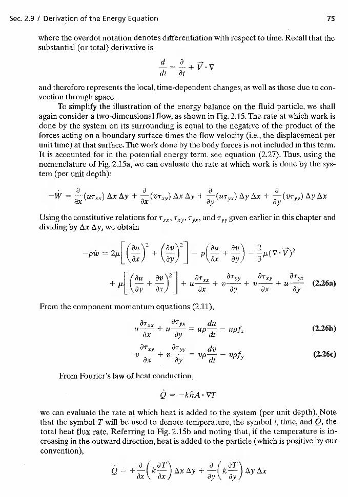
Sec. 2.9 / Derivation of the Energy Equation 75
where the overdot notation denotes differentiation with respect to time. Recall that thesubstantial (or total) derivative is
d 0 —*
dt dt
and therefore represents the local, time-dependent changes, as well as those due to con-vection through space.
To simplify the illustration of the energy balance on the fluid particle, we shallagain consider a two-dimensional flow, as shown in Fig. 2.15. The rate at which work isdone by the system on its surrounding is equal to the negative of the product of theforces acting on a boundary surface times the flow velocity (i.e., the displacement perunit time) at that surface. The work done by the body forces is not included in this term.It is accounted for in the potential energy term, see equation (2.27). Thus, using thenomenclature of Fig. 2.15a, we can evaluate the rate at which work is done by the sys-tem (per unit depth):
—* = + + + iXy
Using the constitutive relations for Txy, Tyx, and given earlier in this chapter anddividing by we obtain
IOu dv\ 2—pw =
+ u—) j —+
—
[IOU dv\21 dTyy dTxy OTyx(226a)
L \ 3y Ox I J dx Oy dx
From the component momentum equations (2.11),
t3Tyx duu— + ii— = up— — (2.26b)dx dt
OTyy dvv + v— vp— — vpf, (2.26c)
dx di'
From Fourier's law of heat conduction,
Q——khA•VT
we can evaluate the rate at which heat is added to the system (per unit depth). Notethat the symbol T will be used to denote temperature, the symbol t, time, and Q, thetotal heat flux rate. Referring to Fig. 2.15b and noting that, if the temperature is in-creasing in the outward direction, heat is added to the particle (which is positive by ourconvention),
of aT\ al aT\0 = +—( k— JtIxAy + —1k-—dx! OyJ
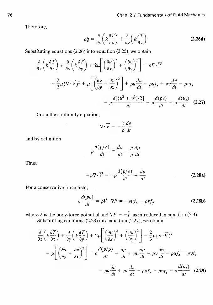
76 Chap. 2 I Fundamentals of Fluid Mechanics
Therefore,
= + (2.26d)t3x) ayJ
Substituting equations (2.26) into equation (2.25), we obtain
a / 3T\ a / aT\ I7au\2 (av\21—lk—)+-—lk-—--J+2p1 (—I +1—Iax) ay) [\t3xJ J
2 2 F/au av\21 du dv
d[(u2 + v2)/2] d(pe) d(iie)= dt
+dt + dt
(2.27)
From the continuity equation,
ldpv.v=-------p dt
and by definition
d(p/p) dp pdpdt dtpdt
Thus,
d(p/p) dp—pV V = —p
dt +(2.28a)
For a conservative force field,
d(pe)= pV VF — (2.28b)
where Fis the body-force potential and VF = —f, as introduced in equation (3.3).Substituting equations (2.28) into equation (2.27), we obtain
++ + -
ax\ ax) ayj [\axl j 3
[(au av\21 d(p/p) dp du dvdt +d+pud+PvdPuhPvfY
du dv d(Ue)= Pu + — — +
dt(2.29)
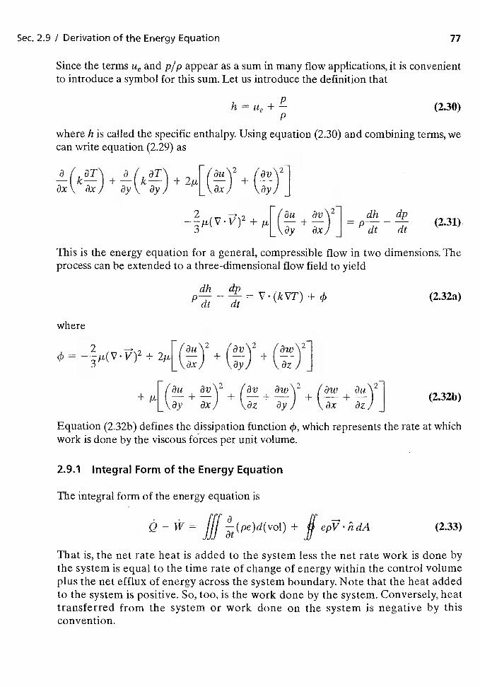
Sec. 2.9 / Derivation of the Energy Equation 77
Since the terms Ue and p/p appear as a sum in many flow applications, it is convenientto introduce a symbol for this sum. Let us introduce the definition that
h = tie + (2.30)p
where h is called the specific enthalpy. Using equation (2.30) and combining terms, wecan write equation (2.29) as
a 7 aT\ a I aT'\ /av\2I—I +1—ax \. 8x) ay \ äy I L \äy
++
= — (2.31).
This is the energy equation for a general, compressible flow in two dimensions. Theprocess can be extended to a three-dimensional flow field to yield
p-—-V(kVT)+çb (2.32a)
where
4) = ++ +
[/'ati av\2 lay aw'\2 I&wI
(232b)L ay az I J
Equation (2.32b) defines the dissipation function 4), which represents the rate at whichwork is done by the viscous forces per unit volume.
2.9.1 Integral Form of the Energy Equation
The integral form of the energy equation is
— =+ if epV.hdA (2.33)
That is, the net rate heat is added to the system less the net rate work is done bythe system is equal to the time rate of change of energy within the control volumeplus the net efflux of energy across the system boundary. Note that the heat addedto the system is positive. So, too, is the work done by the system. Conversely, heattransferred from the system or work done on the system is negative by thisconvention.
Chap. 2 I Fundamentals of Fluid Mechanics
2.9.2 Energy of the System
As noted earlier, the energy of the system can take a variety of forms. They are usuallygrouped as follows:
1. Kinetic energy (ke): energy associated with the directed motion of the mass2. Potential energy (pe): energy associated with the position of the mass in the ex-
ternal field
3. Internal energy (ue): energy associated with the internal fields and the randommotion of the molecules
Thus, the energy of the system may be written as
e = ke + pe + ite (2.34a)
Let us further examine the terms that comprise the energy of the system. The kinetic en-ergy per unit mass is given by
ke = V2 (2.34b)
Note that the change in kinetic energy during a process clearly depends only on the ini-tial velocity and final velocity of the system of fluid particles. Assuming that the exter-nal force field is that of gravity, the potential energy per unit mass is given by
pe = gz (2.34c)
Note that the change in the potential energy depends only on the initial and final ele-vations. Furthermore, the change in internal energy is a function of the values at theendpoints only.
Substituting equations (2.34) into equation (2.33), we obtain
— = + gz + ue)d(vol)
+ if + gz + (2.35)
It should be noted that, whereas the changes in the energy components are a functionof the states, the amount of heat transferred and the amount of work done during aprocess are path dependent. That is, the changes depend not only on the intial and finalstates but on the process that takes place between these states.
Let us consider further the term for the rate at which work is done, W. For conve-nience, the total work rate is divided into flow work rate (Wf), viscous work rate (Wv),and shaft work rate (Wa).
2.9.3 Flow Work
Flow work is the work done by the pressure forces on the surroundings as the fluidmoves through space. Consider flow through the streamtube shown in Fig. 2.16. The
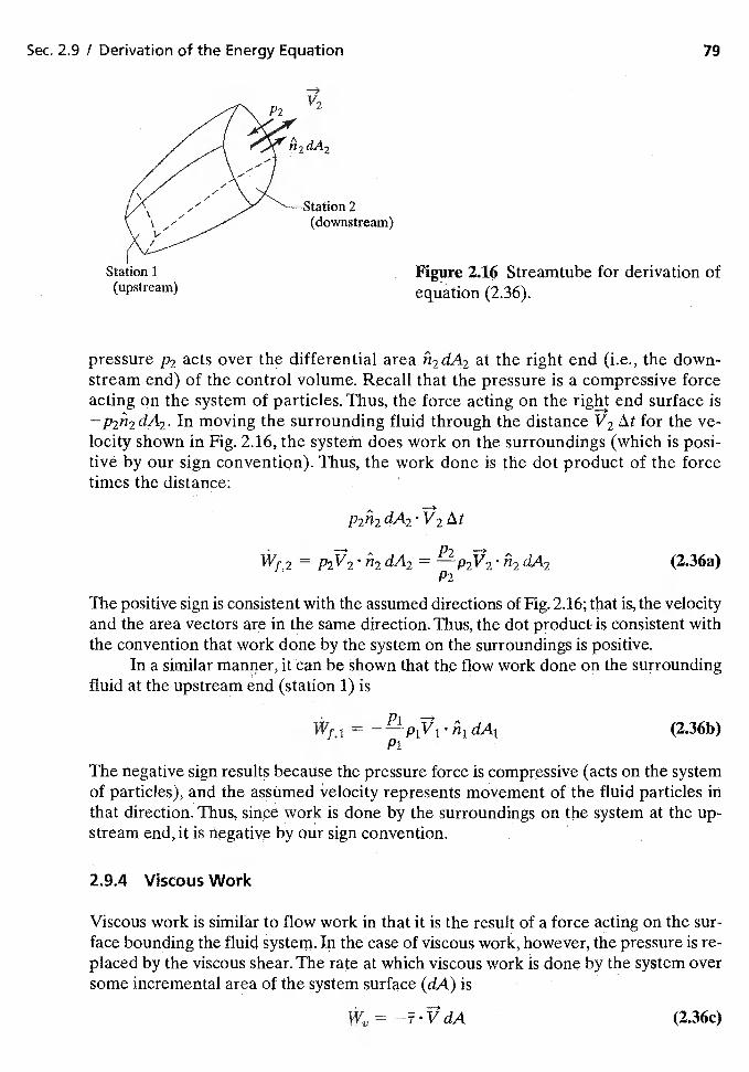
Sec. 2.9 / Derivation of the Energy Equation 79
(downstream)
Figure 2.16 Streamtube for derivation ofequation (2.36).
pressure P2 acts over the differential area ii2dA2 at the right end (i.e., the down-stream end) of the control volume. Recall that the pressure is a compressive forceacting cm the system of particles. Thus, the force acting on the right end surface is—p2n2 dA2. In moving the surrounding fluid through the distance V2 At for the ve-locity shown in Fig. 2.16, the system does work on the surroundings (which is posi-live by our sign convention). Thus, the work done is the dot product of the forcetimes the distance:
p2ii2dA2'V2At
Wf,2 = P2V2 fl2 dA2 = —p2V2 fl2 dA2P2
(2.36a)
The positive sign is consistent with the assumed directions of Fig. 2.16; that is, the velocityand the area vectors are in the same direction. Thus, the dot product is consistent withthe convention that work done by the system on the surroundings is positive.
In a similar manner, it can be shown that the flow work done on the surroundingfluid at the upstream end (station 1) is
P1Wjç1 ——-p1Vj.IuidA1 (2.36b)
The negative sign results because the pressure force is compressive (acts on the systemof particles), and the assumed velocity represents movement of the fluid particles inthat direction. Thus, since work is done by the surroundings on the system at the up-stream end, it is negative by our sign convention.
2.9.4 Viscous Work
Viscous work is similar to flow work in that it is the result of a force acting on the sur-face bounding the fluid system. In the case of viscous work, however, the pressure is re-placed by the viscous shear. The rate at which viscous work is done by the system oversome incremental area of the system surface (dA) is
= —i•VdA (2.36c)
V2P2
(upstream)
80 Chap. 2 / Fundamentals of F'uid Mechanics
2.9.5 Shaft Work
Shaft work is defined as any other work done by the system other than the flow workand the viscous work. This usually enters or leaves the system through the action of ashaft (from which the term originates), which either takes energy out of or puts ener-gy into the system. Since a turbine extracts energy from the system, the system does workon the surroundings and W5 is positive. In the case where the shaft is that of a pump,the surroundings are doing work on the system and is negative.
2.9.6 Application of the Integral Form of the EnergyEquation
Thus, the energy equation can be written
— = Jf/ + gz + Ue)d(VOl)
+ + gz + Ue + (2.37)
Note that the flow work, as represented by equation (2.36), has been incorporated intothe second integral of the right-hand side of equation (2.37).
For a steady, adiabatic flow (Q = 0) with no shaft work (W3 = 0) and with no vis-cous work = 0), equation (2.37) can be written
if p(3- + gz + = 0 (2.38)
where the definition for the enthalpy has been used.
EXAMPLE 2.5: A flow where the energy equation is Bernoulli'sequation
Consider the steady, inviscid, one-dimensional flow of water in the curved pipeshown in Fig. 2.17. If water drains to the atmosphere at station 2 at the rate of0.OOlir m3/s what is the static pressure at station 1? There is no shaft work orheat transfer, and there are no perceptible changes in the internal energy.
Solution: We will apply equation (2.37) to the control volume that encloses the fluidin the pipe between stations 1 and 2. Applying the conditions and assump-tions in the problem statement,
No heat transfer Q = 0
No shaft work = 0
No viscous work = 0
Steady flow = 0at
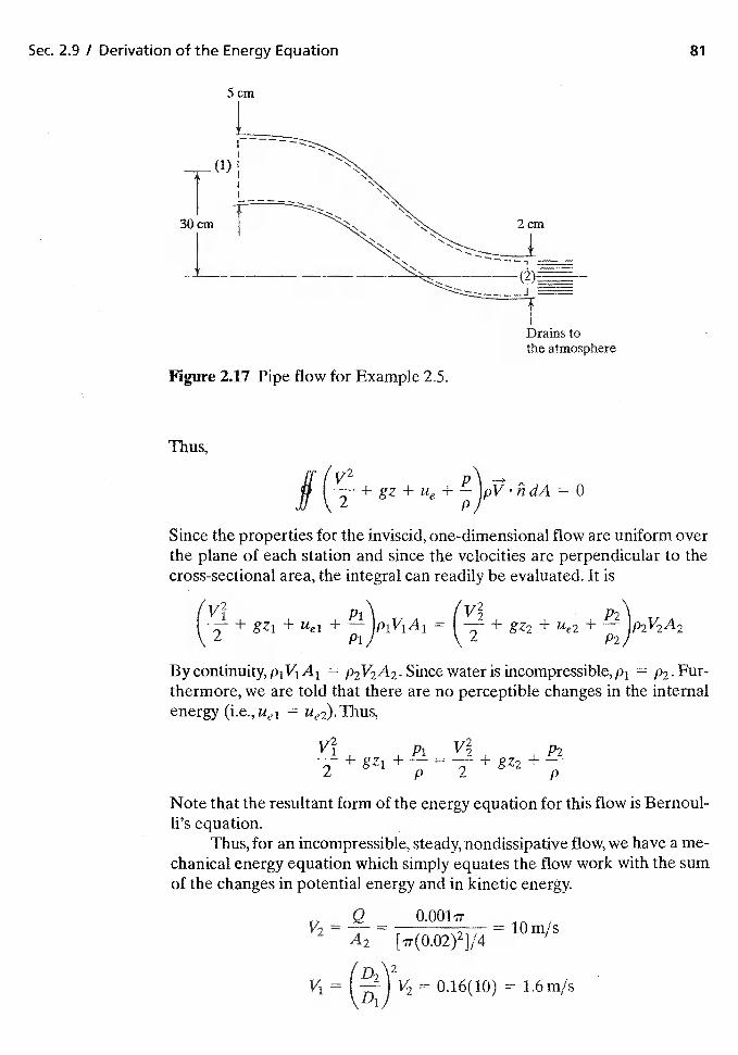
Sec. 2.9 I Derivation of the Energy Equation
5 cm
Drains tothe atmosphere
fff'v2if
Since the properties for the inviscid, one-dimensional flow are uniform overthe plane of each station and since the velocities are perpendicular to thecross-sectional area, the integral can readily be evaluated. It is
/112+ + Uel + )P1V1A1 + gz2 + Ue2 +
2 P1 2 P2
By continuity, p1V1A1 p2V2A2. Since water is incompressible, Pi = P2• Fur-thermore, we are told that there are no perceptible changes in the internalenergy (i.e.,uei = Ue2).ThUS,
Ti2Pi V2 P2
Note that the resultant form of the energy equation for this flow is Bernoul-li's equation.
Thus, for an incompressible, steady, nondissipative flow, we have a me-chanical energy equation which simply equates the flow work with the sumof the changes in potential energy and in kinetic energy.
(D2\2V1 = V2 = 0.16(10) = 1.6 rn/s
\ '-'11
(1)
I30cm
Figure 217 Pipe flow for Example 2.5.
Thus,
QV2 10 rn/s
{ir(0.02)2]/4
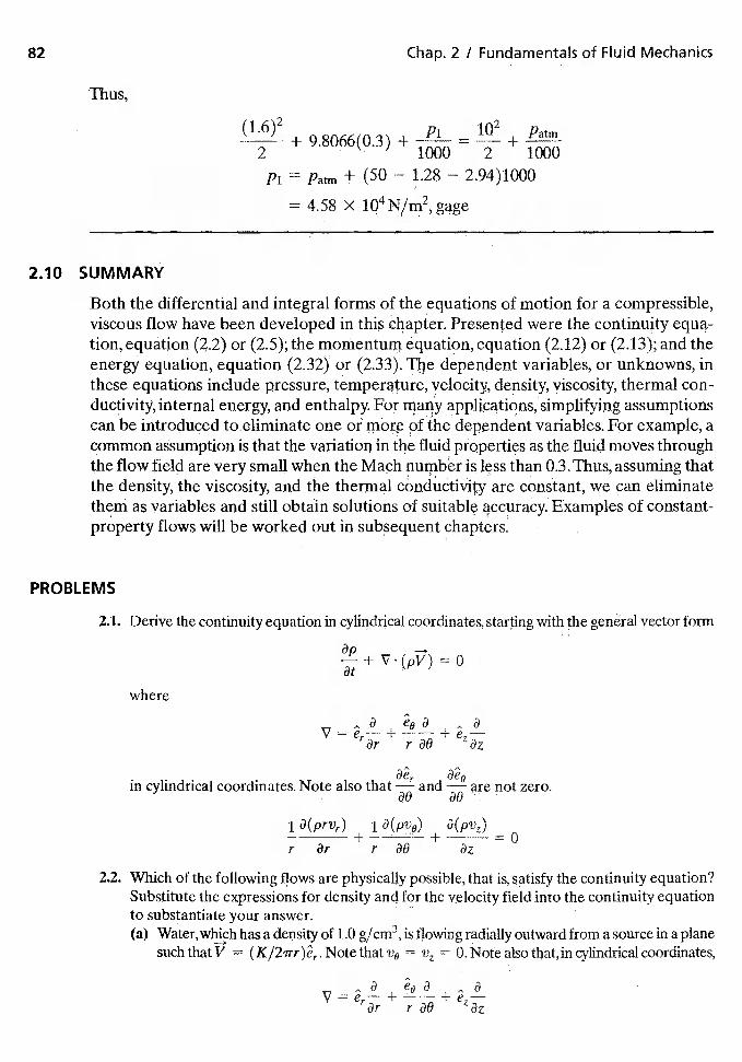
82 Chap. 2 / Fundamentals of Fluid Mechanics
Thus,
11 i\2 2
+ 9 8066(0 3\ + Pi = + Patm
2 ' 1000 2 1000
P1 = Patrn ± (50 — 1.28 2.94)1000
4.58 X N/rn2, gage
2.10 SUMMARY
Both the differential and integral forms of the equations of motion for a compressible,viscous flow have been developed in this chapter. Presented were the continuity equa-tion, equation (2.2) or (2.5); the momentum equation, equation (2.12) or (2.13); and theenergy equation, equation (2.32) or (2.33). T11e dependent variables, or unknowns, inthese equations include pressure, temperature, velocity, density, viscosity, thermal con-ductivity, internal energy, and enthalpy For many applications, simplifying assumptionscan be introduced to ehminate one or more of the dependent variables For example, acommon assumption is that the in the fluid properties as the fluid moves throughthe flow field are very small when the Mach number is less than 0.3.Thus, assuming thatthe density, the viscosity, and the thermal conductivity are constant, we can eliminatethem as variables and still obtain solutions of suitable accuracy Examples of constant-property flows will be worked out in subsequent chapters.
PROBLEMS
2.1. Derive the continuity equation in cylh!drical coordinates, starting with the general vector form
t3p —.+ V.(pV) 0
where
V = er— +3r az
in cylindrical coordinates. Note also that and are not zero.
1 a(prvr) 1 a(pv0)+— + =0r r
2.2. Which of the following flows are physically possible, that is, satisfy the continuity equation?Substitute the expressions for density and for the velocity field into the continuity equationto substantiate your answer.(a) Water,which has a density of 1.0 g,/cm3, is flowing radially outward from a source in a plane
such that V = Note that V9 = = 0. Note also that, in cylindrical coordinates,
V = + -u——- +43r rao az
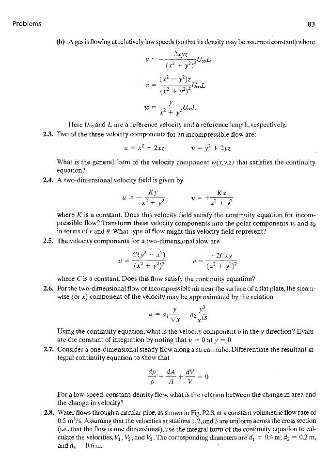
Prob'ems 83
(b) A gas is flowing at relatively low speeds (so that its density may be assumed constant) where
2xyz2U00L
(x2 + y2)
(x2 — y2)z
2x +yHere and L are a reference velocity and a reference length, respectively.
2.3. Two of the three velocity components for an incompressible flow are:
u=x2+2xz v=y2+2yz
What is the general form of the velocity component w(x,y,z) that satisfies the continuityequation?
2.4. A two-dimensional velocity field is given by
Ky KxU—2 2 2x+y x+ywhere K is a constant. Does this velocity field satisfy the continuity equation for incom-pressible flow? Transform these velocity components into the polar components Vr and v8in terms of r and 0. What type of flow might this velocity field represent?
2.5. The velocity components for a two-dimensional flow are
C(y2 — x2) — —2CxyU
(x2 + y2)2V
— (x2 + y2)2
where C is a constant. Does this flow satisfy the continuity equation?2.6. For the two-dimensional flow of incompressible air near the surface of a flat plate, the steam-
wise (or x) component of the velocity may be approximated by the relation
y y3U = —
Using the continuity equation, what is the velocity component v in the y direction? Evalu-ate the constant of integration by noting that v = 0 at y 0.
2.7. Consider a one-dimensional steady flow along a streamtube. Differentiate the resultant in-tegral continuity equation to show that
dp dA dV
p A V
For a low-speed, constant-density flow, what is the relation between the change in area andthe change in velocity?
2.8. Water flows through a circular pipe, as shown in Fig. P2.8, at a constant volumetric flow rate of0.5 m3/s, Assuming that the velocities at stations 1,2, and 3 are uniform across the cross section(i.e., that the flow is one dimensional), use the integral form of the continuity equation to cal-culate the velocities, V1, V2, and V3. The corresponding diameters are d1 = 0.4 m, d2 = 0.2 m,andd3 = O.6m.
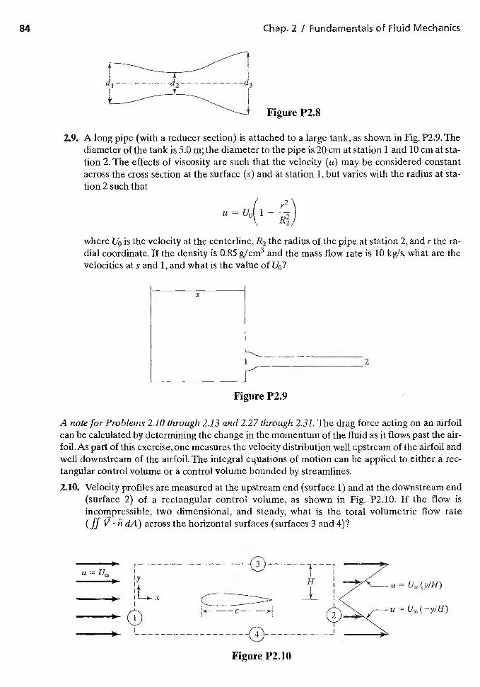
Chap. 2 / Fundamentals of Fluid Mechanics
d3
Figure P2.8
2.9. A long pipe (with a reducer section) is attached to a large tank, as shown in Fig. P2.9.Thediameter of the tank is 5.0 m; the diameter to the pipe is 20 cm at station 1 and 10 cm at sta-tion 2. The effects of viscosity are such that the velocity (it) may be considered constantacross the cross section at the surface (s) and at station 1, but varies with the radius at sta-tion 2 such that
= u0(i—
where U0 is the velocity at the centerline, R2 the radius of the pipe at station 2, and r the ra-dial coordinate. If the density is 0.85 g/cm3 and the mass flow rate is 10 kg/s, what are thevelocities at s and 1, and what is the value of U0?
S
1 2
Figure P2.9
A note for Problems 2.10 through 2.13 and 2.27 through 2.31. The drag force acting on an airfoilcan be calculated by determining the change in the momentum of the fluid as it flows past the air-foil. As part of this exercise, one measures the velocity distribution well upstream of the airfoil andwell downstream of the airfoil. The integral equations of motion can be applied to either a rec-tangular control volume or a control volume bounded by streamlines.
2.10. Velocity profiles are measured at the upstream end (surface 1) and at the downstream end(surface 2) of a rectangular control volume, as shown in Fig. P2.10. If the flow isincompressible, two dimensional, and steady, what is the total volumetric flow rate(if V - del) across the horizontal surfaces (surfaces 3 and 4)?
Kc
I
Figure P2.19
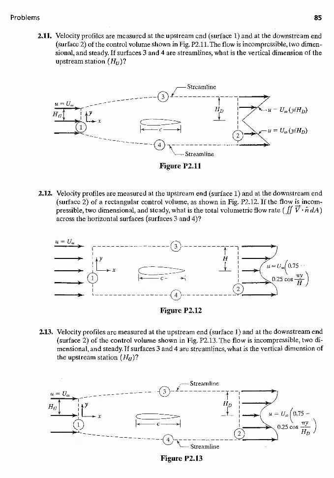
Problems 85
2.11. Velocity profiles are measured at the upstream end (surface 1) and at the downstream end(surface 2) of the control volume shown in Fig. P2.11. The flow is incompressible, two dimen-sional, and steady. If surfaces 3 and 4 are streamlines, what is the vertical dimension of theupstream station (He)?
=U(/HD
)
Streamline
Figure P2.11
2.12. Velocity profiles are measured at the upstream end (surface 1) and at the downstream end(surface 2) of a rectangular control volume, as shown in Fig. P2.12. If the flow is incom-pressible, two dimensional, and steady, what is the total volumetric flow rate (if V ci dA)across the horizontal surfaces (surfaces 3 and 4)?
U =
Figure P2.12
2.13. Velocity profiles are measured at the upstream end (surface 1) and at the downstream end(surface 2) of the control volume shown in Fig. P2.13. The flow is incompressible, two di-mensional, and steady. If surfaces 3 and 4 are streamlines, what is the vertical dimension ofthe upstream station (He)?
Streamline
U = - I
C
C
k c
Figure P2.13
)
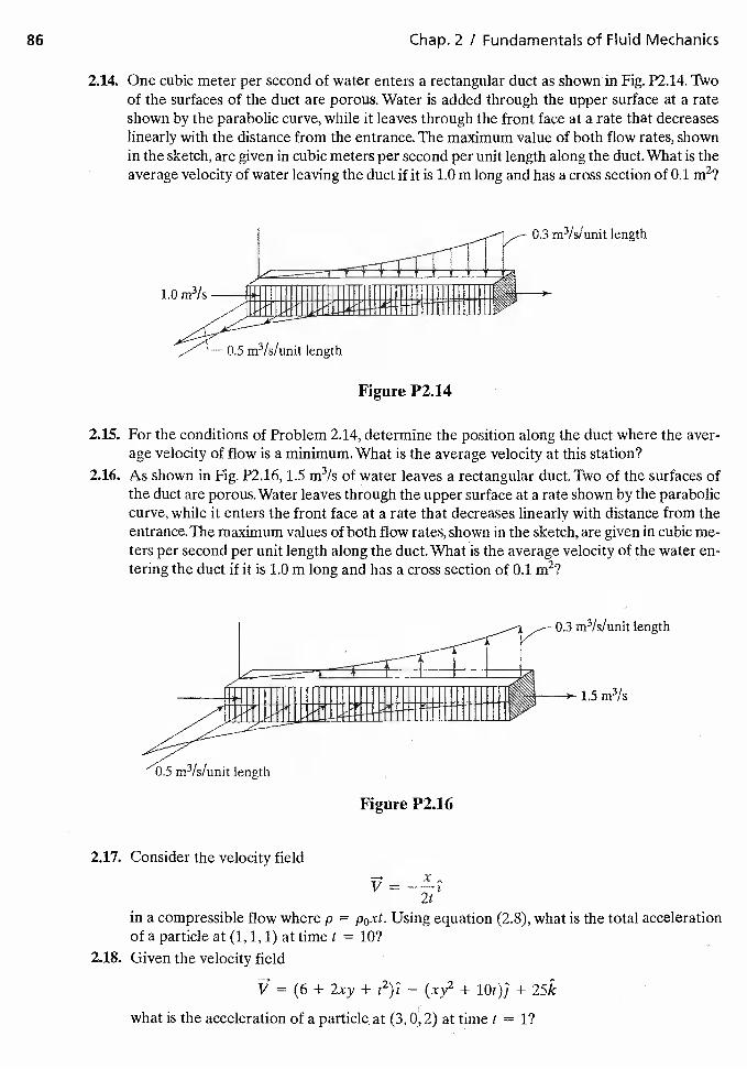
86 Chap. 2 I Fundamentals of Fluid Mechanics
2.14. One cubic meter per second of water enters a rectangular duct as shown in Fig. P2.14. Twoof the surfaces of the duct are porous. Water is added through the upper surface at a rateshown by the parabolic curve, while it leaves through the front face at a rate that decreaseslinearly with the distance from the entrance. The maximum value of both flow rates, shownin the sketch, are given in cubic meters per second per unit length along the duct. What is theaverage velocity of water leaving the duct if it is 1.0 m long and has a cross section of 0.1 m2?
ft3 m3/s/unit length
2.15. For the conditions of Problem 2.14, determine the position along the duct where the aver-age velocity of flow is a minimum. What is the average velocity at this station?
2.16. As shown in Fig. P2.16, 1.5 m3Is of water leaves a rectangular duct. Two of the surfaces ofthe duct are porous. Water leaves through the upper surface at a rate shown by the paraboliccurve, while it enters the front face at a rate that decreases linearly with distance from theentrance. The maximum values of both flow rates, shown in the sketch, are given in cubic me-ters per second per unit length along the duct. What is the average velocity of the water en-tering the duct if it is 1,0 m long and has a cross section of 0,1 m2?
2.17. Consider the velocity field
V=---iin a compressible flow where p = p0xt. Using equation (2.8), what is the total accelerationof a particle at (1,1, 1) at time t = 10?
2.18. Given the velocity field
V = (6 + 2xy + — (xy2 + lOt)j + 25k
what is the acceleration of a particle at (3, 2) at time t = 1?
1.0 m3/s
0.5 m3/s/unit length
Figure P2.14
m3lslunit length
1.5 ni3ls
Figure P2.16
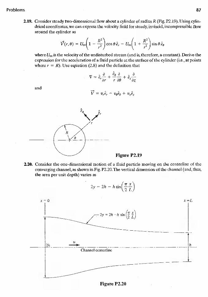
Problems 87
2.19. Consider steady two-dimensional flow about a cylinder of radius R (Fig. P2.19). Using cylin-drical coordinates, we can express the velocity field for steady, inviscid, incompressible flowaround the cylinder as
f R2\ / R2\V(r,O) = U00( 1 )coSOer — 1 + Jsinoè9
" TI TIwhere is the velocity of the undisturbed stream (and is, therefore, a constant). Derive theexpression for the acceleration of a fluid particle at the surface of the cylinder (i.e., at pointswhere T = R). Use equation (2.8) and the definition that
and
V = + —— +ar T80
V = + +
Figure P2.19
2.20. Consider the one-dimensional motion of a fluid particle moving on the centerline of theconverging channel, as shown in Fig. P2.20.The vertical dimension of the channel (and, thus,the area per unit depth) varies as
2y = 2/i
Figure P2.20
x=O x =L
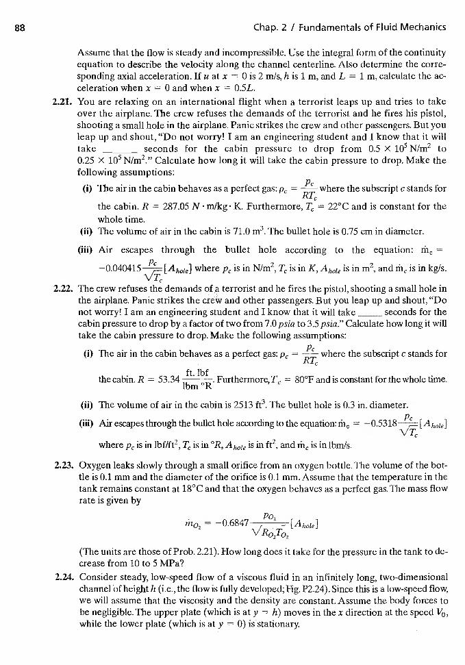
88 Chap. 2 / Fundamentals of Fluid Mechanics
Assume that the flow is steady and incompressible. Use the integral form of the continuityequation to describe the velocity along the channel centerline. Also determine the corre-sponding axial acceleration. If u at x = 0 is 2 mIs, h is 1 m, and L = 1 m, calculate the ac-celeration when x 0 and when x = Q.5L.
2.21. You are relaxing on an international flight when a terrorist leaps up and tries to takeover the airplane. The crew refuses the demands of the terrorist and he fires his pistol,shooting a small hole in the airplane. Panic strikes the crew and other passengers. But youleap up and shout, "Do not worry! I am an engineering student and I know that it willtake
_______
seconds for the cabin pressure to drop from 0.5 X N/rn2 to0.25 X N/rn2." Calculate how long it will take the cabin pressure to drop. Make thefollowing assumptions:
(i) The air in the cabin behaves as a perfect gas: Pc = where the subscript c stands for
the cabin. R = 287.05 N . m/kg K. Furthermore, = 22°C and is constant for thewhole time.
(ii) The volume of air in the cabin is 71.0 m3. The bullet hole is 0.75 cm in diameter.
(iii) Air escapes through the bullet hole according to the equation: =
where Pc is in N/rn2, is in K, is in m2, and is in kg/s.
2.22. The crew refuses the demands of a terrorist and he fires the pistol, shooting a small hole inthe airplane. Panic strikes the crew and other passengers. But you leap up and shout, "Donot worry! I am an engineering student and I know that it will take seconds for thecabin pressure to drop by a factor of two from 7.0 psia to 3.5 psia." Calculate how long it willtake the cabin pressure to drop. Make the following assumptions:
(i) The air in the cabin behaves as a perfect gas: where the subscript c stands for
ft. lbfthe cabm. R = 53.34 . Furthermore, = 80°F and is constant for the whole time.
ibm °R
(ii) The volume of air in the cabin is 2513 ft3. The bullet hole is 0.3 in. diameter.
(iii) Air escapes through the bullet hole according to the equation: = {Aho!e]
where is in lbf/ft2, is in °R, A hole is in ft2. and is in lbmls.C
2.23. Oxygen leaks slowly through a small orifice from an oxygen bottle. The volume of the bot-tle is 0.1 mm and the diameter of the orifice is 0.1 mm. Assume that the temperature in thetank remains Constant at 18°C and that the oxygen behaves as a perfect gas. The mass flowrate is given by
Po2m02 = —0.6847 ,-_____{Ah018]
V R02T0,
(The units are those of Prob. 2.21). How long does it take for the pressure in the tank to de-crease from 10 to 5 MPa?
2.24. Consider steady, low-speed flow of a viscous fluid in an infinitely long, two-dimensionalchannel of height h (i.e., the flow is fully developed; Fig. P2.24). Since this is a low-speed flow,we will assume that the viscosity and the density are constant. Assume the body forces tobe negligible. The upper plate (which is at y = h) moves in the x direction at the speed V0,while the lower plate (which is at y = 0) isstationary.
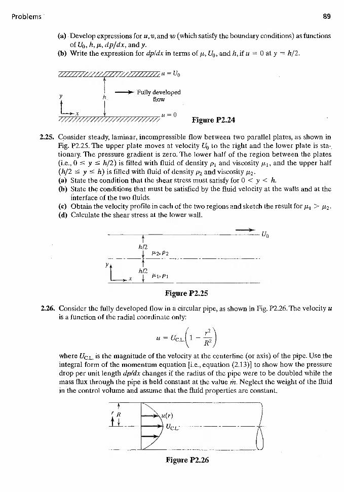
Problems 89
(a) Develop expressions for u, v, and w (which satisfy the boundary conditions) as functionsof U0, h, p., dp/dx, andy.
(b) Write the expression for dp/dx in terms of p., U0, and h, if u = 0 at y = h/2,
U = U0
) Fully developed
2.25. Consider steady, laminar, incompressible flow between two parallel plates, as shown inFig. P2.25. The upper plate moves at velocity U0 to the right and the lower plate istionary. The pressure gradient is zero. The lower half of the region between the plates.(i.e., 0 � y � h/2) is filled with fluid of density P1 and viscosity and the upper half(h/2 � y � h) is filled with fluid of density P2 and viscosity p.2.(a) State the condition that the shear stress must satisfy for 0 < y < h.(b) State the conditions that must be satisfied by the fluid velocity at the walls and at the
interface of the two fluids.(c) Obtain the velocity profile in each of the two regions and sketch the result for >(d) Calculate the shear stress at the lower wall.
th/2
t___h/2
y
Figure P2.25
2.26. Consider the fully developed flow in a circular pipe, as shown in Fig. P2.26. The velocity uis a function of the radial coordinate only:
= uCL(1—
where UCL is the magnitude of the velocity at the centerline (or axis) of the pipe. Use theintegral form of the momentum equation [i.e., equation (2.13)] to show how the pressuredrop per unit length dp/dx changes if the radius of the pipe were to be doubled while themass flux through the pipe is held constant at the value rh. Neglect the weight of the fluidin the control volume and assume that the fluid properties are constant.
Figure P2.26
y
Figure P2.24
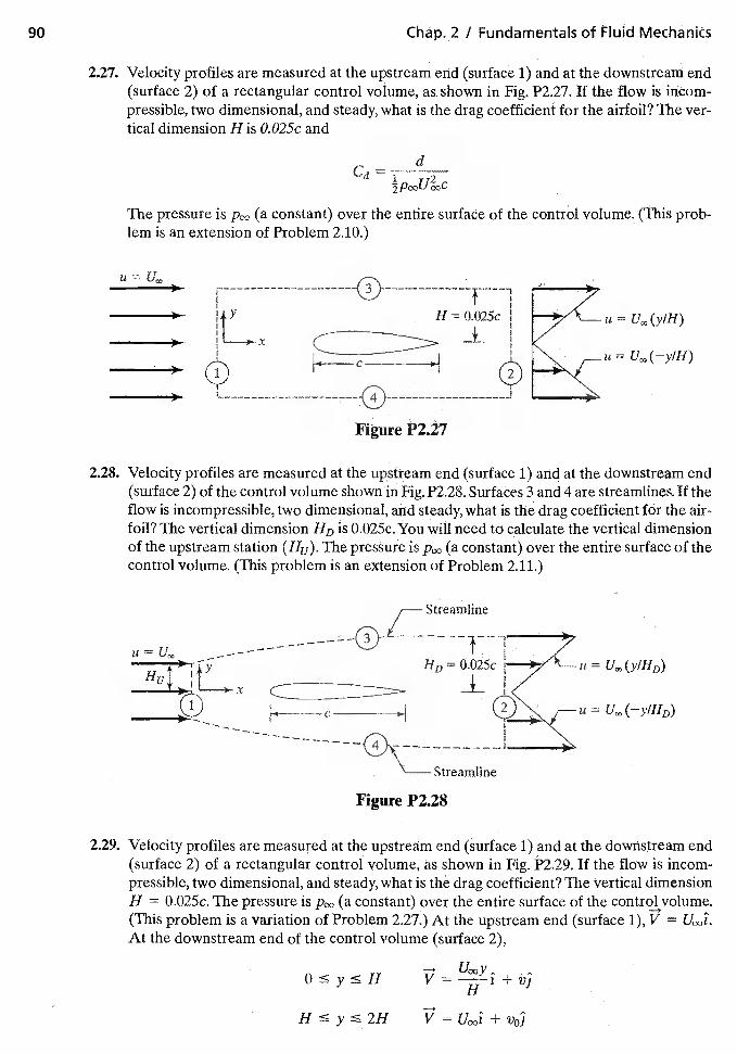
90 Chap. 2 I Fundamentals of Fluid Mechanics
2.27. Velocity profiles are measured at the upstream (surface 1) and at the downstream end(surface 2) of a rectangular control volume, as. shown in Fig. P2.27. If the flow is incom-pressible, two dimensional, and steady, what is the drag coefficient for the airfoil? The ver-tical dimension H is O.025c and
dCd—
The pressure is (a constant) over the entire surface of the control volume. (This prob-lem is an extension of Problem 2.10.)
II F1 IY H = O.025c u = U0, (ytH)
I K.. - U - /H0,( )
Figure P2.27
2.28. Velocity profiles are measured at the upstream end (surface 1) and at the downstream end(surface 2) of the control volume shown in Fig. P2.28. Surfaces 3 and 4 are streamlines. If theflow is incompressible, two dimensional, and steady, what is the drag coefficient fOr the air-foil? The vertical dimension HD is 0.025c. You will need to calculate the vertical dimensionof the upstream station (Hu). The pressure is (a constant) over the entire surface of thecontrol volume. (This problem is an extension of Problem 2.11.)
Streamline
:1.:.
U0,(—y/HD)
j___Streamline
Figure P2.28
2.29. Velocity profiles are measured at the upstream end (surface 1) and at the downstream end(surface 2) of a rectangular control volume, as shown in Fig. P2,29. If the flew is incom-pressible, two dimensional, and steady, what is the drag coefficient? The vertical dimensionH = 0.025c. The pressure is (a constant) over the entire surface of the(This problem is a variation of Problem 2.27.) At the upstream end (surface 1), VAt the downstream end of the control volume (surface 2),
0cy�H
H
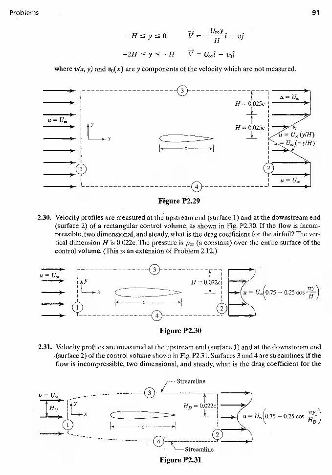
Problems 91
where v(x, y) and v0(x) are y components of the velocity which are not measured.
)r I H=0.025c
p H=0.025c
C
Figure P2.29
2.30. Velocity profiles are measured at the upstream end (surface 1) and at the downstream end(surface 2) of a rectangular control volume, as shown in Fig. P2.30. If the flow is incom-pressible, two dimensional, and steady, what is the drag coefficient for the airfoil? The ver-tical dimension H is 0.022c. The pressure is (a constant) over the entire surface of thecontrol volume. (This is an extension of Problem 2.12.)
U = [ ®- II Y H=0022c
) x — 0.25
c(1)
-0-Figure P2.30
2.31. Velocity profiles are measured at the upstream end (surface 1) and at the downstream end(surface 2) of the control volume shown in Fig. P2.31. Surfaces 3 and 4 are streamlines. If theflow is incompressible, two dimensional, and steady, what is the drag coefficient for the
i— Streamline
U =
t11 P /u 1
= — 0.25 cos
1 C
i"— Streamline
Figure P2.31
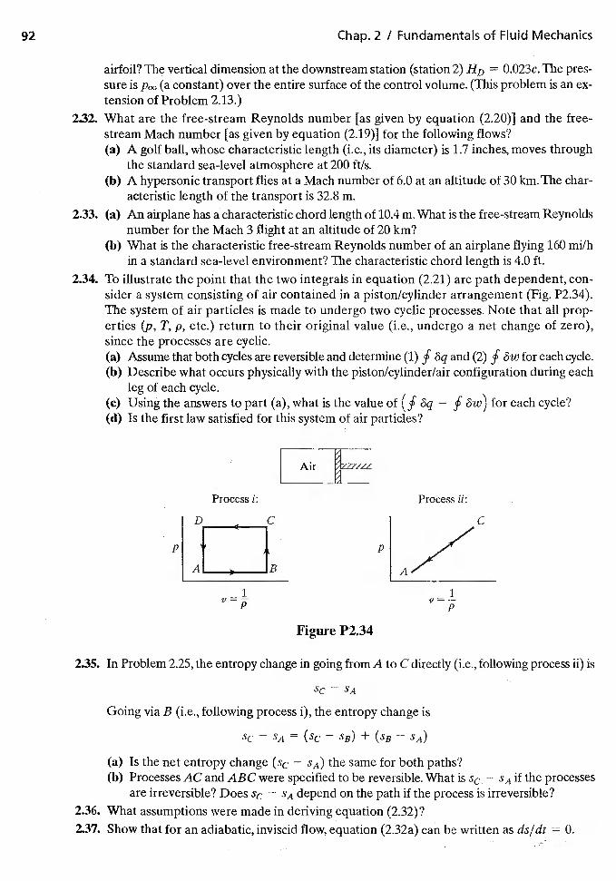
92 Chap. 2 / Fundamentals of Fluid Mechanics
airfoil? The vertical dimension at the downstream station (station 2) HD = 0.023c. The pres-sure is (aconstant) over the entire surface of the control volume. (This problem is an ex-tension of Problem 2.13.)
2.32. What are the free-stream Reynolds number [as given by equation (2.20)] and the free-stream Mach number [as given by equation (2.19)] for the following flows?(a) A golf ball, whose characteristic length (i.e., its diameter) is 1.7 inches, moves through
the standard sea-level atmosphere at 200 ft/s.(b) A hypersonic transport flies at a Mach number of 6.0 at an altitude of 30 km. The char-
acteristic length of the transport is 32.8 m.
2.33. (a) An airplane has a characteristic chord length of 10.4 m. What is the free-stream Reynoldsnumber for the Mach 3 flight at an altitude of 20 km?
(b) What is the characteristic free-stream Reynolds number of an airplane flying 160 mi/hin a standard sea-level environment? The characteristic chord length is 4.0 ft.
2.34. To illustrate the point that the two integrals in equation (2.21) are path dependent, con-sider a system consisting of air contained in a piston/cylinder arrangement (Fig. P2.34).The system of air particles is made to undergo two cyclic processes. Note that all prop-erties (p. T, p, etc.) return to their original value (i.e., undergo a net change of zero),since the processes are cyclic.(a) Assume that both cycles are reversible and determine (1) 6q and (2) f 6w for each cycle.(b) Describe what occurs physically with the piston/cylinder/air configuration during each
leg of each cycle.(c) Using the answers to part (a), what is the value of (j 6q — j for each cycle?(d) Is the first law satisfied for this system of air particles?
Air
Process i: Process ii:
Figure P2.34
235. In Problem 2.25, the entropy change in going from A to C directly (i.e., following process ii) is
SC SA
Going via B (i.e., following process i), the entropy change is
SCSA(SCSB)+(SBSA)(a) Is the net entropy change (SC — SA) the same for both paths?(ii) Processes AC and ABC were specified to be reversible. What is se-. — SA if the processes
are irreversible? Does SC — 5A depend on the path if the process is irreversible?2.36. What assumptions were made in deriving equation (2.32)?2.37. Show that for an adiabatic, inviscid flow, equation (2.32a) can be written as ds/dt = 0.
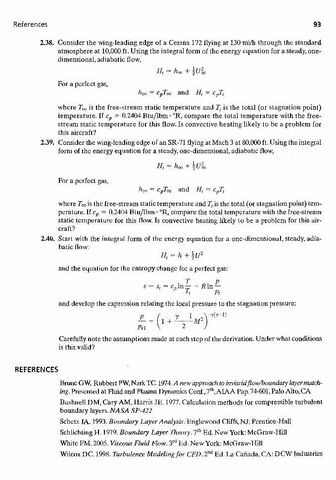
References 93
2.38. Consider the wing-leading edge of a Cessna 172 flying at 130 mi/h through the standardatmosphere at 10,000 ft. Using the integral form of the energy equation for a steady, one-dimensional, adiabatic flow,
For a perfect gas,= and H1
where is the free-stream static temperature and T1 is the total (or stagnation point)temperature. If cAf, = 0.2404 Btu/lbm °R, compare the total temperature with the free-stream static temperature for this flow. Is convective heating likely to be a problem forthis aircraft?
2,39. Consider the wing-leading edge of an SR-71 flying at Mach 3 at 80,000 ft. Using the integralform of the energy equation for a steady, one-dimensional, adiabatic flow,
H1 = +
For a perfect gas,= and H1 =
where is the free-stream static temperature and is the total (or stagnation point) tem-perature. If = 0.2404 Btu/lbm °R, compare the total temperature with the free-streamstatic temperature for this flow. Is convective heating likely to be a problem for this air-craft?
2.40. Start with the integral form of the energy equation for a one-dimensional, steady, adia-batic flow:
H1 = h +
and the equation for the entropy change for a perfect gas:
T ps — = — Rln—
T1 Pt
and develop the expression relating the local pressure to the stagnation pressure:
P / -y 1—=(1+ M2Pti \. 2
Carefully note the assumptions made at each step of the derivation. Under what conditionsis this valid?
REFERENCES
Brune GW, Rubbert PW, NarkTC. 1974. A new approach to inviwidflow/boundaiy layer match-ing. Presented at Fluid and Plasma Dynamics Conf., 7th, AIAA Pap. 74-601, Palo Alto, CA
Bushnell DM, Cary AM, Harris JE. 1977. Calculation methods for compressible turbulentboundary layers. NASA SP-422
Schetz JA. 1993. Boundary Layer Analysis. Englewood Cliffs, NJ: Prentice-Hall
Schlichting H. 1979. Boundary Layer Theory. 7th Ed. New York: McGraw-Hill
White FM. 2005. Viscous Fluid Flow. Ed. New York: McGraw-Hill
Wilcox DC. 1998. Turbulence Modeling for CFD. Ed. La Canada, CA: DCW Industries
3 DYNAMICS OFANINCOMPRESSIBLE,
INVISCID FLOW FIELD
As will be discussed in Chapter 14, for many applications, solutions of the inviscid regioncan provide important design information. Furthermore, once the inviscid flow field hasbeen defined, it can be used as boundary conditions for a thin, viscous boundary layeradjacent to the surface. For the majority of this text, the analysis of the flow field willmake use of a two-region flow model (one region in which the viscous forces are negli-gible, i.e., the inviscid region, and one in which viscous forces cannot be neglected, i.e.,the viscous boundary layer near the surface).
3.1 INVISCID FLOWS
As noted in Chapter 2, the shearing stresses may be expressed as the product of theviscosity times the shearing stress velocity gradient. There are no real fluids for whichthe viscosity is zero. However, there are many situations where the product of theviscosity times the shearing velocity gradient is sufficiently small that the shear-stressterms may be neglected when compared to the other terms in the governing equations.Let us use the term inviscid flow to describe the flow in those regions of the flow fieldwhere the viscous shear-stresses are negligibly small. By using the term inviscid flowinstead of inviscid fluid, we emphasize that the viscous shear stresses are small becausethe combined product of viscosity and the shearing velocity gradients has a small effecton the flow field and not that the fluid viscosity is zero. In fact, once the solution for the
94
Sec. 3.2 I Bernoufli's Equation 95
inviscid flow fIeld is Obtained, the eiigineer may want to solve the boundary-layerequations and calculate the skin friction drag on the configuration.
Inregions of the flow field where the viscOus shear stresses are negligibly small (i.e.,in regions where the flow is inviscid), equation (2.12) becomes
du apph — (3la)
= — (3.lb)
dw 3p— — (3.lc)
In vector form, the equatiOn is
—, 1(3.2)
No assumption has been made about density, so these equations apply to a com-pressible flow as well as to an incompressible one. These equations, derived in 1755by Eulef, are called the Euler equations.
In this chapter we develop fundamental conCepts for describing the flow aroundconfigurations in a low-speed stream. Let us assume that the viscous boundary layer isthin and thetefore has a negligible influence on the inviscid flow field. (The effect ofviolating this assumpiioh will be discussed when we compare theoretical results with
We will seek the solution for the inviscid portion of the flow field (i.e., the flowoutside the boundary layer). The momentum equation is Euler's equation.
3.2 BERNOULLI'S EQUATION
As has been discussed, the density is essentially constant when the gas particles in theflow field move at relatively low speeds or when the fluid is a liquid. Further, let usconsider only body forces that are cOnservative (such as is the case for gravity),
f=—VF (3.3)
and flows that are steady (or steady state):
Using the vector identity that
(U2\
equation (3.2) becomes (for these assumptions)
(3.4)
96 Chap. 3 / Dynamics of an Incompressible, Inviscid Flow Field
In these equations U is the scalar magnitude of the velocity V. Consideration of thesubsequent applications leads us to use U (rather than V).
Let us calculate the change in the magnitude of each of these terms along an arbitrarypath whose length and direction are defined by the vector ds. To do this, we take the dotproduct of each term in equation (3.4) and the vector ds. The result is
/ 2\I (4i+ dF+ — V X (V X V).ds = 0 (3.5)
Note that, since V x (V x V) is a vector perpendicular to V, the last term is zero(1) for any displacement if the flow is irrotational (i.e., where V x V = 0), or (2) fora displacement along a streamline if the flow is rotational. Thus, for a flow that is
1. Inviscid,2. Incompressible,3. Steady, and4. Irrotational (or, if the flow is rotational, we consider only displacements along a
streamline), and for which5. The body forces are conservative,
the first integral of Euler's equation is
f ± f dF + / = constant (3.6)
Since each term involves an exact differential,
u2 p+ F + constant (3.7)
2 p
The force potential most often encountered is that due to gravity. Let us take the z axisto be positive when pointing upward and normal to the surface of the earth. The forceper unit mass due to gravity is directed downward and is of magnitude g. Therefore,referring to equation (3.3),
soF = gz (3.8)
The momentum equation becomes
u2+ gz + constant (3.9)
2 p
Equation (3.9) 'is known as Bernoulli's equation.Because the density has been assumed constant, it is not necessary to include
the energy equation in the procedure to solve for the velocity and pressure fields. Infact, equation (3.9), which is a form of the momentum equation, can be derived from
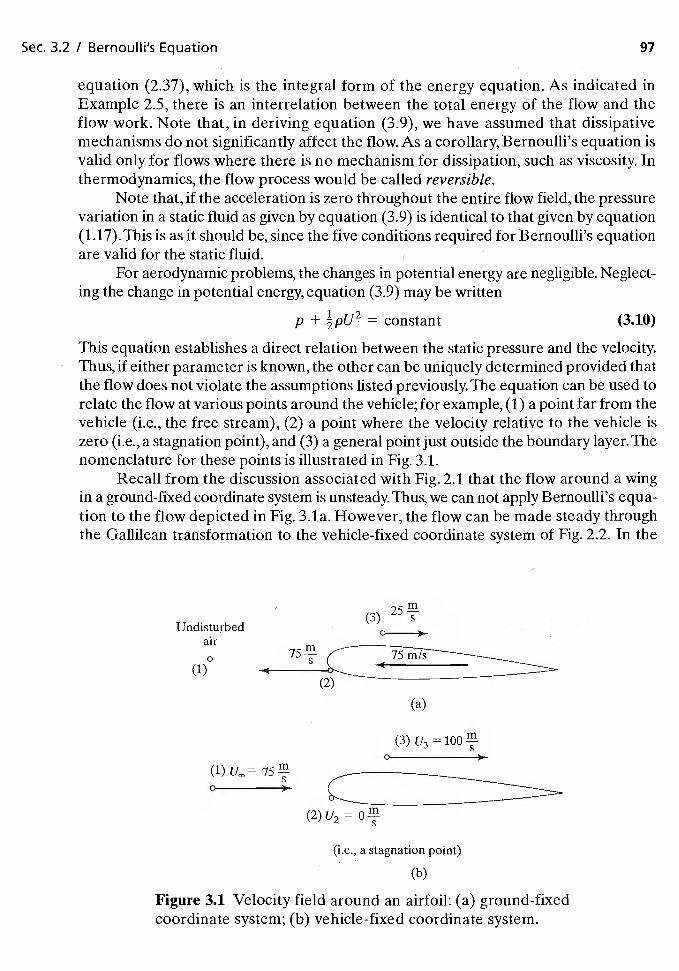
Sec. 3.2 / Bernoulli's Equation 97
equation (2.37), which is the integral form of the energy equation. As indicated inExample 2.5, there is an interrelation between the total energy of the flow and theflow work. Note that, in deriving equation (3.9), we have assumed that dissipativemechanisms do not significantly affect the flow. As a corollary, Bernoulli's equation isvalid only for flows where there is no mechanism for dissipation, such as viscosity. Inthermodynamics, the flow process would be called reversible.
Note that, if the acceleration is zero throughout the entire flow field, the pressurevariation in a static fluid as given by equation (3.9) is identical to that given by equation(1.17).This is as it should be, since the five conditions required for Bernoulli's equationare valid for the static fluid.
For aerodynamic problems, the changes in potential energy are negligible. Neglect-ing the change in potential energy, equation (3.9) may be written
p + = constant (3.10)
This equation establishes a direct relation between the static pressure and the velocity.Thus, if either parameter is known, the other can be uniquely determined provided thatthe flow does not violate the assumptions listed previously. The equation can be used torelate the flow at various points around the vehicle; for example, (1) a point far from thevehicle (i.e., the free stream), (2) a point where the velocity relative to the vehicle iszero (i.e., a stagnation point), and (3) a general point just outside the boundary layer. Thenomenclature for these points is illustrated in Fig. 3.1.
Recall from the discussion associated with Fig. 2.1 that the flow around a wingin a ground-fixed coordinate system is unsteady.Thus, we can not apply Bernoulli's equa-tion to the flow depicted in Fig. 3.la. However, the flow can be made steady throughthe Gallilean transformation to the vehicle-fixed coordinate system of Fig. 2.2. In the
(3)Undisturbed
_______
(1)°
(a)
U3
(1)U,,=75!'!
(2)U2 =
(i.e., a stagnation point)
(b)
Figure 3.1 Velocity field around an airfoil: (a) ground-fixedcoordinate system; (b) vehicle-fixed coordinate system.
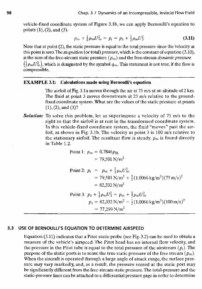
98 Chap. 3 I Dynamics of an Incompressible, lnvisdd Flow Field
vehicle-fixed coordinate system of Figure 3.lb, we can apply Bernoulli's equation topoints (1), (2), and (3).
1 — — I rr2
Note that at.point (2), the static pressure is equal to the total pressure since the velocity atthis point is zero.The stagnation (ortotal)pressure,which is the constant of equation (3.10),is the sum of the free-stream static pressure and the free-stream dynamic pressure
which is designated by the symbol This statement is not true, if the flow iscompressible.
EXAMPLE 3.1: Calculations made using Bernoulli's equation
The airfoil of Fig. 3.la moves through the air at 75 mIs at an altitude of 2 km.The flUid at point 3 moves downstream at 25 rn/s relative to the ground-fixed coordinate system. What are the values of the static pressure at points(1), (2), and (3)?
Solution: To solve this problem, let us superimpose a velocity of 75 m/s to theright so that the airfoil is at rest in the transformed coordinate system.In this vehicle-fixed coordinate system, the fluid "moves" past the air-foil, as shown in 3.lb. The velocity at point 3 is 100 m/s relative tothe stationary airfoil. The resultant flow is steady. is found directlyin Table 1.2.
Point 1: pc,o = °.7846P5L
79,501 N/rn2
Point 2: = +
= 79,501 N/rn2 + (1.0066 kg/m3)(75 m/s)2
= 82,332 N/rn2
- 1 rr2 — 1 rT2romLJ. P3 2P00U13 m
p3 = 82,332N/m2 —
= 77,299 N/rn2
3.3 USE OF BERNOULLI'S EQUATION TO DETERMINE AIRSPEED
Equation (3.11) indicates that a Pitot-static probe (see Fig. 3.2) can be used to obtain ameasure of the vehicle's airspeed. The Pitot head has no internal flow velocity, andthe pressure in the Pitot ttibe is equal to the total pressure of the airstrearn (p,). Thepurpose of the static ports is to sense the true static pressure of the free streamWhen the aircraft is operated through a large angle of attack range, the surface pres-sure may vary markedly, and, as a result, the pressure sensed at the static port maybe significantly different from the free-stream static pressure. The total-pressure and thestatic-pressure lines can be attached to a differential pressure gage in order to determine
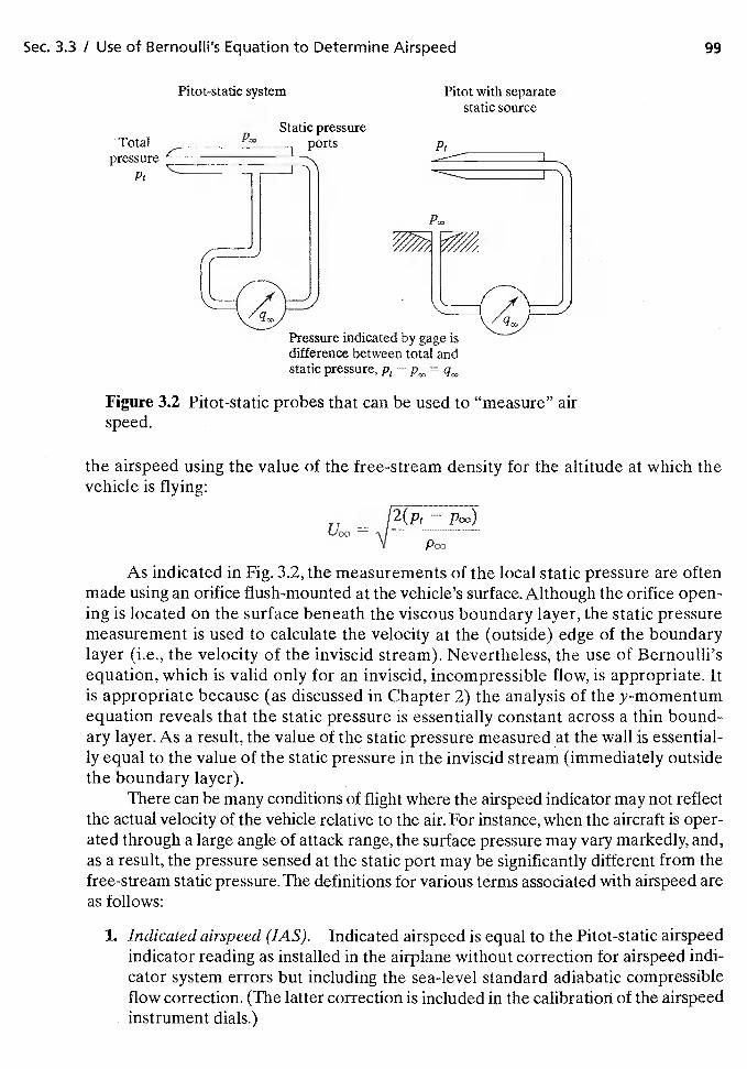
Sec. 3.3 I Use of Bernoulti's Equation to Determine Airspeed 99
Pitot-static system Pitot with separatestatic source
Static pressureTotal ports
pressurePt
Pressure indicated by gage isdifference between total andstatic pressure, — =
Figure 3.2 Pitot-static probes that can be used to "measure" airspeed.
the airspeed using the value of the free-stream density for the altitude at which thevehicle is flying:
As indicated in Fig. 3.2, the measurements of the local static pressure are oftenmade using an orifice flush-mounted at the vehicle's surface. Although the orifice open-ing is located on the surface beneath the viscous boundary layer, the static pressuremeasurement is used to calculate the velocity at the (outside) edge of the boundarylayer (i.e., the velocity of the inviscid stream). Nevertheless, the use of Bernoulli'sequation, which is valid only for an inviscid, incompressible flow, is appropriate. Itis appropriate because (as discussed in Chapter 2) the analysis of the y-momentumequation reveals that the static pressure is essentially constant across a thin bound-ary layer. As a result, the value of the static pressure measured at the wall is essential-ly equal to the value of the static pressure in the inviscid stream (immediately outsidethe boundary layer).
There can be many conditions of flight where the airspeed indicator may not reflectthe actual velocity of the vehicle relative to the air. For instance, when the aircraft is oper-ated through a large angle of attack range, the surface pressure may vary markedly, and,as a result, the pressure sensed at the static port may be significantly different from thefree-stream static pressure. The definitions for various terms associated with airspeed areas follows:
1. Indicated airspeed (lAS). Indicated airspeed is equal to the Pitot-static airspeedindicator reading as installed in the airplane without correction for airspeed indi-cator system errors but including the sea-level standard adiabatic compressibleflow correction. (The latter correction is included in the calibration of the airspeedinstrument dials.)
Pt
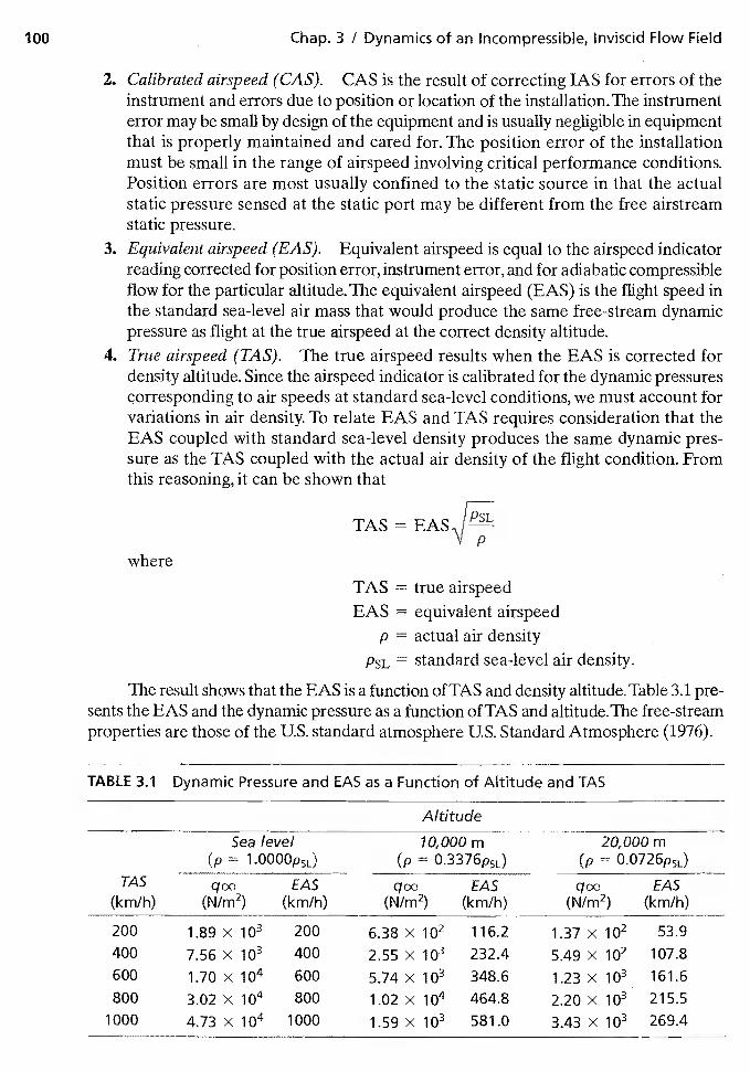
Chap. 3 / Dynamics of an Incompressible, Inviscid Flow Field
2. Calibrated airspeed (CAS). CAS is the result of correcting lAS for errors of theinstrument and errors due to position or location of the installation. The instrumenterror may be small by design of the equipment and is usually negligible in equipmentthat is properly maintained and cared for. The position error of the installationmust be small in the range of airspeed involving critical performance conditions.Position errors are most usually confined to the static source in that the actualstatic pressure sensed at the static port may be different from the free airstreamstatic pressure.
3. Equivalent airspeed (EAS). Equivalent airspeed is equal to the airspeed indicatorreading corrected for position error, instrument error, and for adiabatic compressibleflow for the particular altitude. The equivalent airspeed (EAS) is the flight speed inthe standard sea-level air mass that would produce the same free-stream dynamicpressure as flight at the true airspeed at the correct density altitude.
4. True airspeed (TAS). The true airspeed results when the EAS is corrected fordensity altitude. Since the airspeed indicator is calibrated for the dynamic pressurescorresponding to air speeds at standard sea-level conditions, we must account forvariations in air density. To relate EAS and TAS requires consideration that theEAS coupled with standard sea-level density produces the same dynamic pres-sure as the TAS coupled with the actual air density of the flight condition. Fromthis reasoning, it can be shown that
TAS =
EAS = airspeedair density
PSL = standard sea-level air density.
The result shows that the EAS is a function of TAS and density altitude. Table 3.1 pre-sents the EAS and the dynamic pressure as a function of TAS and altitude.The free-streamproperties are those of the U.S. standard atmosphere U.S. Standard Atmosphere (1976).
TABLE 3.1 Dynamic Pressure and EAS as a Function of Altitude and TAS
Altitude
Sea level(p = l.0000psi)
10,000 m(p =
20,000 m(p =
TAS
(km/h)qcx EAS
(N/rn2) (km/h)qco EAS
(N/rn2) (km/h)qcx EAS
(N/rn2) (km/h)
200 1.89 x 200 6.38 X 116.2 1.37 x 53.9400 7.56 x 400 2.55 x i03 232.4 5,49 x 107.8
600800
1.70 x i04 600
3.02 x 8005.74 x i03 348.6
1.02 x 464,81.23 x 161.6
2.20 >< 215.51000 4.73 x 1000 1.59 >< io3 581.0 3,43 x iQ3 269.4
Sec. 3.4 / The Pressure Coefficient
3.4 THE PRESSURE COEFFICIENT
The engineer often uses experimental data or theoretical solutions for one flow condi-tion to gain insight into the flow field which exists at another flow condition. Wind-tun-nel data, where scale models are exposed to flow conditions that simulate the designflight environment, are used to gain insight to describe the full-scale flow field at otherflow conditions. Therefore, it is most desirable to present (experimental or theoretical)correlations in terms of dimensionless coefficients which depend only upon the config-uration geometry and upon the angle of attack. One such dimensionless coefficient is thepressure coefficient, which is defined as
1 ir2 (.In flight tests and wind-tunnel tests, pressure orifices, which are located flush mountedin the surface, sense the local static pressure at the wall [p in equation (3.12)]. Never-theless, these experimentally determined static pressures, which are located beneaththe viscous boundary layer, can be presented as the dimensionless pressure coefficientusing equation (3.12).
If we consider those flows for which Bernoulli's equation applies, we can expressthe pressure coefficient in terms of the nondimensionalized local velocity. Rearrangingequation (3.11),
1
Treating point 3 as a general point in the flow field, we can write the pressure coef-ficient as
(3.13)
Thus, at the stagnation point, where the local velocity is zero, = = 1.0 for an in-compressible flow. Note that the stagnation-point value is independent of the free-streamflow conditions or the configuration geometry.
EXAMPLE 3.2: Flow in an open test-section wind tunnel
Consider flow in a subsonic wind tunnel with an open test section; that is,the region where the model is located is open to the room in which the tun-nel is located. Thus, as shown in Fig. 3.3, the air accelerates from a reservoir(or stagnation chamber) where the velocity is essentially zero, through aconverging nozzle, exhausting into the room (i.e., the test section) in a uni-form, parallel stream of velocity Using a barometer located on the wallin the room where the tunnel is located, we know that the barometric pres-sure in the room is 29.5 in Hg.
The model is a cylinder of infinite span (i.e., the dimension normalto the paper is infinite).There are two pressure orifices flush with the wind-tunnel walls and two orifices flush with the model surface, as shown inFigure 3.3. The pressure sensed at orifice 3, which is at the stagnation point
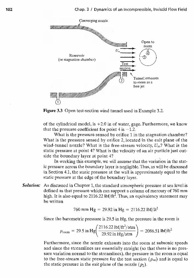
102 Chap. 3 / Dynamics of an Incompressible, Inviscid Flow Field
Converging nozzle
OoReservoir
(or stagnation chamber)
_________
Testsection
a Tunnel exhausts2 toroomasa
free jet
Figure 3.3 Open test-section wind tunnel used in Example 3.2.
of the cylindrical model, is +2.0 in of water, gage. Furthermore, we knowthat the pressure coefficient for point 4 is —1.2.
What is the pressure sensed by orifice 1 in the stagnation chamber?What is the pressure sensed by orifice 2, located in the exit plane of thewind-tunnel nozzle? What is the free-stream velocity, What is thestatic pressure at point 4? What is the velocity of an air particle just out-side the boundary layer at point 4?
In working this example, we will assume that the variation in the stat-ic pressure across the boundary layer is negligible. Thus, as will be discussedin Section 4.1, tl1e static pressure at the wall is approximately equal to thestatic pressure at the edge of the boundary layer.
Solution: As discussed in Chapter 1, the standard atmospheric pressure at sea level isdefined as that pressure which can support a column of mercury of 760 mmhigh. It is also equal to 2116.22 lbf/ft2. Thus, an equivalency statement maybe written
760 mm Hg 29.92 in Hg = 2116.22 lbf/ft2
Since the barometric pressure is 29.5 in Hg, the pressure in the room is
(2116.22 lbf/ft2/atm\Prnorn = 29.5 in
29.92 in Hg/atm )= 2086.51 lbf/ft2
Furthermore, since the nozzle exhausts into the room at subsonic speedsand since the streamlines are essentially straight (so that there is no pres-sure variation normal to the streamlines), the pressure in the room is equalto the free-stream static pressure for the test section and is equal tothe static pressure in the exit plane of the nozzle (p2).
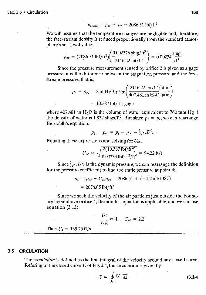
Sec. 3.5 / Circulation 103
Proorn = Pcx P2 2O86.51 Ibf/ft2
We will assume that the temperature changes are negligible and, therefore,the free-stream density is reduced proportionally from the standard atmos-phere's sea-level value:
(0.002376 slug/ft3\ slu= (2086.51 lbf/ft2)( I = 0.00234—
\ 2116.22 lbf/ft2 J ft3
Since the pressure measurement sensed by orifice 3 is given as a gagepressure, it is the difference between the stagnation pressure and the free-stream pressure, that is,
(2116.22 lbf/ft2/atm— 2 in H20,
gage
in H20 is the column of water equivalent to 760 mm Hg ifthe density of water is 1.937 slugs/ft3. But since = Pt' we can rearrangeBernoulli's equation:
P3 P Pt PaEquating these expressions and solving for
T2(1o.387 lbf/ft2)= I = 94.22 ft/s
V 0.00234 lbf• s2/ft4
Since is the dynamic pressure, we can rearrange the definitionfor the pressure coefficient to find the static pressure at point 4:
+ = 2086.51 + (—1.2)(10.387)
= 2074.05 lbf/ft2
Since we seek the velocity of the air particles just outside the bound-ary layer above orifice 4, Bernoulli's equationis applicable, and we can useequation (3.13):
Thus, U4 = 139.75 ft/s.
3.5 CIRCULATION
The circulation is defined as the line integral of the velocity around any closed curve.Refering to the closed curve C of Fig. 3.4, the circulation is given by
-T (3.14)
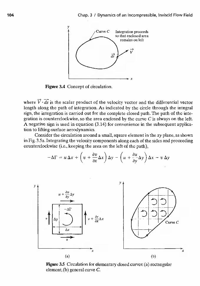
Curve C Integration proceedsso that enclosed area
remains on left
Figure 34 Concept of circulation.
—where V ds is the scalar product of the velocity vector and the differential vectorlength along the path of integration. As indicated by the circle through the integralsign, the integration is carried out for the complete closed path. The path of the inte-gration is counterclockwise, so the area enclosed by the curve C is always on the left.A negative sign is used in equation (3.14) for convenience in the subsequent applica-tion to lifting-surface aerodynamics.
Consider the circulation around a small, square element in the xy plane, as shownin Fig. 3.5a. Integrating the velocity components along each of the sides and proceedingcounterclockwise (i.e., keeping the area on the left of the path),
—IXI' + (v + —
U +
Figure 3.5 Circulation for elementary closed curves: (a) rectangularelement; (b) general curve C.
104 Chap. 3 / Dynamics of an Incompressible, Invisdd Flow Field
y
V
x
yy
Vt4-
f +Curve C
(a)
x
(b)
x
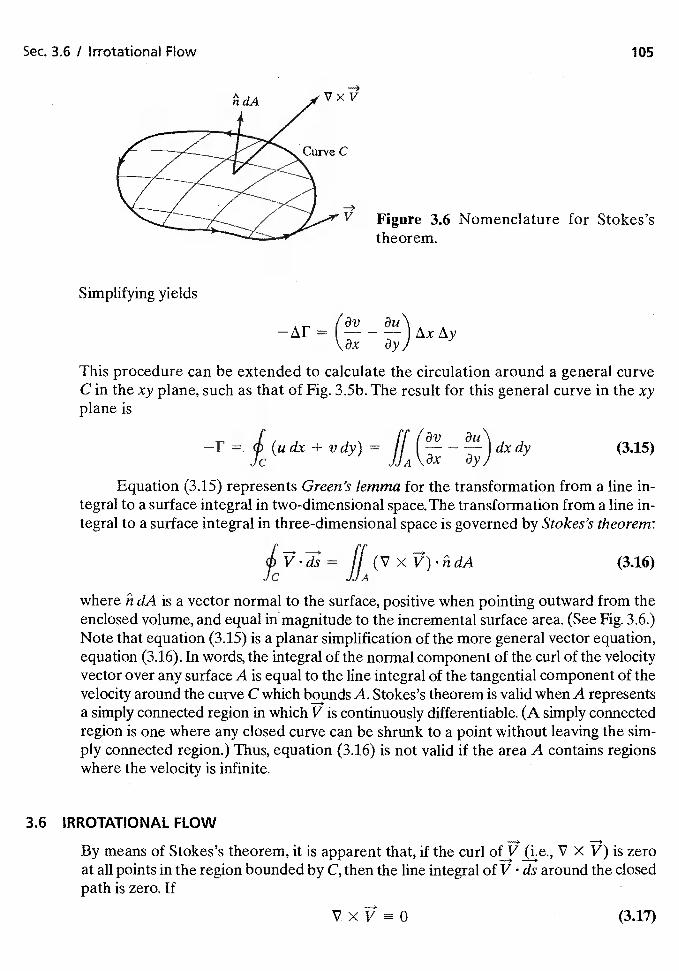
Sec. 3.6 / Irrotational Flow 105
Figure 3.6 Nomenclature for Stokes'stheorem.
= —\\ax t9yJ
This procedure can be extended to calculate the circulation around a general curveC in the xy plane, such as that of Fig. 3.5b. The result for this general curve in the xyplane is
(3.15)
Equation (3.15) represents Green's lemma for the transformation from a line in-tegral to a surface integral in two-dimensional space. The transformation from a line in-tegral to a surface integral in three-dimensional space is governed by Stokes's theorem:
= ff (V x i7) dA (3.16)
where h dA is a vector normal to the surface, positive when pointing outward from theenclosed volume, and equal in magnitude to the incremental surface area. (See Fig. 3.6.)Note that equation (3.15) is a planar simplification of the more general vector equation,equation (3.16). In words, the integral of the normal component of the curl of the velocityvector over any surface A is equal to the line integral of the tangential component of thevelocity around the curve C which bounds A. Stokes's theorem is valid when A representsa simply connected region in which V is continuously differentiable. (A simply connectedregion is one where any closed curve can be shrunk to a point without leaving the sim-ply connected region.) Thus, equation (3.16) is not valid if the area A contains regionswhere the velocity is infinite.
3.6 IRROTATIONAL FLOW
By means of Stokes's theorem, it is apparent that, if the curl of V X V) is zeroat all points in the region bounded by C, then the line integral of V ds around the closedpath is zero. If
(3.17)
vxv
-4V
Simplifying yields
106 Chap. 3 I Dynamics of an Incompressible, Inviscid Flow Field
and the flow contains no singularities, the flow is said to be irrotational. Stokes's theo-rem leads us to the conclusion that
For this irrotational velocity field, the line integral
is independent of path. A necessary and sufficient condition that
be independent of path is that the curl of V is everywhere zero. Thus, its value dependsonly on its limits. However, a line integral can be independent of the path of integrationonly if the integrand is an exact differential. Therefore,
= d4) (3.18)
where d4) is an exact differential. Expanding equation (3.18) in Cartesian coordinates,
84) 84) 84)udx + vdy + wdz = —dx + —dy + —dz
It is apparent that
(3.19)
Thus, a velocity potential 4)(x, y, z) exists for this flow such that the partial derivativeof 4) in any direction is the velocity component in that direction. That equation (3.19)is a valid representation of the velocity field for an irrotational flow can be seen bynoting that
Vx (3.20)
That is, the curl of any gradient is necessarily zero, Thus, an irrotational flow is termeda potential flow.
3.7 KELVIN'S THEOREM
Having defined the necessary and sufficient condition for the existence of a flow that hasno circulation, let us examine a theorem first demonstrated by Lord Kelvin. For an in-viscid, barotropic flow with conservative body forces, the circulation around a closedfluid line remains constant with respect to time. A barotropic flow (sometimes called ahomogeneous flow) is one in which the density depends only on the pressure.
The time derivative of the circulation along a closed fluid line (i.e., a fluid line thatis composed of the same fluid particles) is

Sec. 3.7 / Kelvin's Theorem 107
dr dl=
V ds) ds + V (ds) (3.21)
Again, the negative sign is used for convenience, as discussed in equation (3.14). Euler'sequation, equation (3.2), which is the momentum equation for an inviscid flow, yields
Using the constraint that the body forces are conservative (as is true for gravity, thebody force of most interest to the readers of this text), we have
f=—VFand
= —VF — (3.22)
where Fis the body-force potential. Since we are following a particular fluid particle, theorder of time and space differentiation does not matter.
/ds\= dV (3.23)
Substituting equations (3.22) and (3.23) into equation (3.21) yields
d I IdpV ds = — dF — + V dV (3.24)Ic Jc P Ic
Since the density is a function of the pressure only, all the terms on the right-hand sideinvolve exact differentials. The integral of an exact differential around a closed curve iszero. Thus,
( .
= 0 (3.25)
Or, as given in the statement of Kelvin's theorem, the circulation remains constant alongthe closed fluid line for the conservative flow.
3.7.1 Implication of Kelvin's Theorem
If the fluid starts from rest, or if the velocity of the fluid in some region is uniform andparallel, the rotation in this region is zero. Kelvin's theorem leads to the important con-clusion that the entire flow remains irrotational in the absence of viscous forces and ofdiscontinuities provided that the flow is barotropic and the body forces can be describedby a potential function.
In many flow problems (including most of those of interest to the readers of thistext), the undisturbed, free-stream flow is a uniform parallel flow in which there are noshear stresses. Kelvin's theorem implies that, although the fluid particles in the subsequent
108 Chap. 3 I Dynamics of an Incompressible, Inviscid Flow Field
flow patterns may follow curved paths, the flow remains irrotational except in those re-gions where the dissipative viscous forces are an important factor.
3.8 INCOMPRESSIBLE, IRROTATIONAL FLOW
Kelvin's theorem states that for an inviscid flow having a conservative force field, thecirculation must be constant around a path that moves so as always to touch the sameparticles and which contains no singularities. Thus, since the free-stream flow is irrota-tional, a barotropic flow around the vehicle will remain irrotational provided that vis-cous effects are not important. For an irrotational flow, the velocity may be expressedin terms of a potential function;
V = (3.19)
For relatively low speed flows (i.e., incompressible flows), the continuity equation is
(2.4)
Note that equation (2.4) is valid for a three-dimensional flow as well as a two-dimensionalflow.
Combining equations (2.4) and (3.19), one finds that for an incompressible, irro-tational flow,
V24) = 0 (3.26)
Thus, the governing equation, which is known as Laplace's equation, is a linear, second-order partial differential equation of the elliptic type.
3.8.1 Boundary Conditions
Within certain constraints on geometric slope continuity, a bounded, simply connectedvelocity field is uniquely determined by the distribution on the flow boundaries eitherof the normal component of the total velocity V4) or of the total potential 4). Theseboundary-value problems are respectively designated Neumann or Dirichlet problems. Forapplications in this book, the Neumann formulation will be used since most practical casesinvolve prescribed normal velocity boundary conditions. Specifically, the flow tangencyrequirement associated with inviscid flow past a solid body is expressed mathematically as
because the velocity component normal to the surface is zero at a solid surface.
3.9 STREAM FUNCTION IN A TWO-DIMENSIONAL,INCOMPRESSIBLE FLOW
Just as the condition of irrotationality is the necessary and sufficient condition for theexistence of a velocity potential, so the equation of continuity for an incompressible,two-dimensional flow is the necessary and sufficient condition for the existence of astream function.The flow need be two dimensional only in the sense that it requires only
Sec. 3.9 / Stream Function in a Two-Dimensional, Incompressible Flow
two spatial coordinates to describe the motion. Therefore, stream functions exist bothfor plane flow and for axially symmetric flow. The reader might note, although it is notrelevant to this chapter, that stream functions exist for compressible, two-dimensionalflows, if they are steady.
Examining the continuity equation for an incompressible, two-dimensional flow inCartesian coordinates,
—p du dvv,v = + = 0dx 3y
It is obvious that the equation is satisfied by a stream function for which the velocitycomponents can be calculated as
(3.27a)
ml,v = (3.27b)
dx
A corollary to this is the existence of a stream function is a necessary condition for a phys-ically possible flow (i.e., one that satisfies the continuity equation).
Since i,li is a point function,
dcli = +dx
so that
thji = —v dx + u dy (3.28a)
Since a streamline is a curve whose tangent at every point coincides with the directionof the velocity vector, the definition of a streamline in a two-dimensional flow is
dx — dv
U — V
Rearranging, it can be seen that
udy—vdx——0 (3.28b)
along a streamline. Equating equations (3.28a) and (3.28b), we find that
dcli = 0
along a streamline. Thus, the change in cli is zero along a streamline or, equivalently, i/i isa constant along a streamline. A corollary statement is that lines of constant cl are stream-lines of the flow. It follows, then, that the volumetric flow rate (per unit depth) betweenany two points in the flow is the difference between the values of the stream functionat the two points of interest.
Referring to Fig. 3.7, it is clear that the product v(—dx) represents the volumetricflow rate per unit depth across AG and the product u dy represents the volumetric flow rateper unit depth across GB. By continuity, the fluid crossing lines AG and GB must cross the
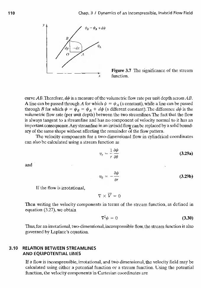
vxV=o
I/lB I/IA +dI/J
A
Chap. 3 / Dynamics of an Incompressible, Inviscid Flow Field
y
________________________
Figure 3.7 The significance of the streamx function.
curve AB.Therefore, is a measure of the volumetric flow rate per unit depth across AB.A line can be passed through A for which = (a constant), while a line can be passedthrough B for which = = + dt/i (a different constant).The difference dtfi is thevolumetric flow rate (per unit depth) between the two streamlines. The fact that the flowis always tangent to a and has no component of velocity normal to it has animportant consequence. Any streamline in an inviscid can be replaced by a solid bound-ary of the same shape without affecting the remainder of the flow pattern.
The velocity components for a two-dimensional flow in cylindrical coordinatescan also be calculated using a stream function as
Vr = (3.29a)
and
VU = — (3.29b)
If the flow is irrotational,
Then writing the velocity components in terms of the stream function, as defined inequation (3.27), we obtain
= 0 (3.30)
Thus, for an irrotational, two-dimensional, incompressible flow, the stream function is alsogoverned by Laplace's equation.
3.10 RELATION BETWEEN STREAMLINESAND EQUIPOTENTIAL LINES
If a flow is incompressible, irrotational, and two dimensional, the velocity field may becalculated using either a potential function or a stream function. Using the potentialfunction, the velocity components in Cartesian coordinates are
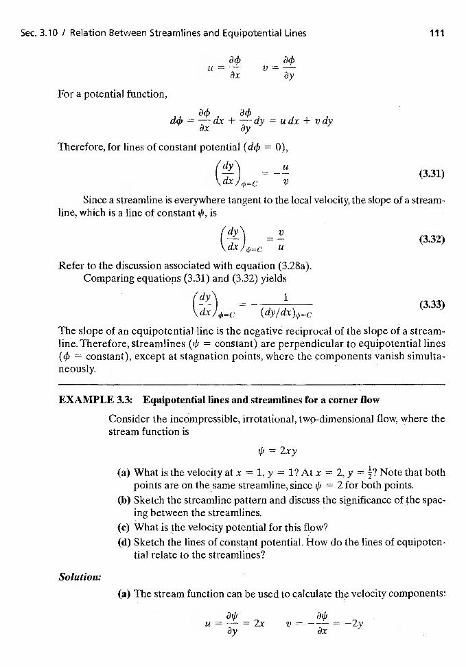
Sec. 3.10 / Relation Between Streamlines and Equipotential Lines
34) 34)u=—3y
For a potential function,
34) 34)dçb = —dx + —dy = udx + vdy
3y
Therefore, for lines of constant potential (d4) 0),
(dy'\ u1—J =—— (331)
V
Since a streamline is everywhere tangent to the local velocity, the slope of a stream-line, which is a line of constant 4), is
=(3.32)
U
Refer to the discussion associated with equation (3.28a).Comparing equations (3.31) and (3.32) yields
(dy\ 11—) = — (3.33)
The slope of an equipotential line is the negative reciprocal of the slope of a stream-line. Therefore, streamlines (4' = constant) are perpendicular to equipotential lines(4) = constant), except at stagnation points, where the components vanish simulta-neously.
EXAMPLE 3.3: Equipotential lines and streamlines for a corner flow
Consider the incompressible, irrotational, two-dimensional flow, where thestream function is
4) = 2xy
(a) What is the velocity at x =1, y = 1? At x 2, y = Note that bothpoints are on the same streamline, since 4) = 2 for both points.
(b) Sketch the streamline pattern and discuss the significance of the spac-ing between the streamlines.
(c) What is the velocity potential for this flow?(d) Sketch the lines of constant potential. How do the lines of equipoten-
tial relate to the streamlines?
Solution:
(a) The stream function can be used to calculate the velocity components:
34' 34)u = — = 2x v —---- —2y
dx
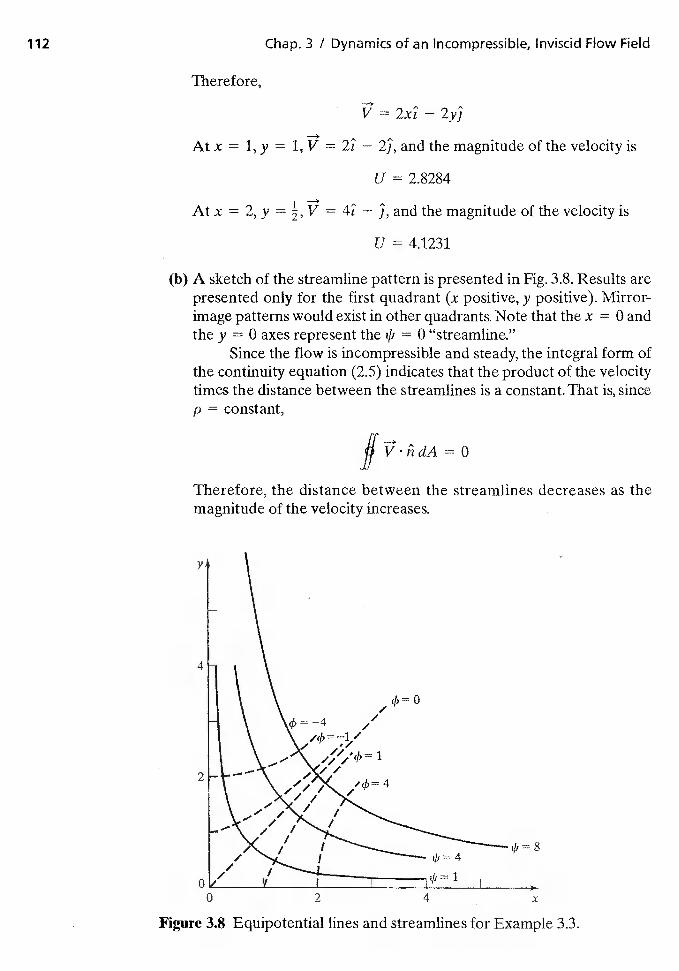
Therefore,
Chap. 3 I Dynamics of an Incompressible, Inviscid Flow Field
V 2x1 — 2yj
At x = 1, y = 1, V = 21 — 21, and the magnitude of the velocity is
U = 2.8284
At x = 2, y = V = 41 — and the magnitude of the velocity is
U = 4.1231
(b) A sketch of the streamline pattern is presented in Fig. 3.8. Results arepresented only for the first quadrant (x positive, y positive). Mirror-image patterns would exist in other quadrants. Note that the x 0 andthe y = 0 axes represent the = 0 "streamlineS"
Since the flow is incompressible and steady, the integral form ofthe continuity equation (2.5) indicates that the product of the velocitytimes the distance between the streamlines is a constant. That is, sincep = constant,
0
Therefore, the distance between the streamlines decreases as themagnitude of the velocity increases.
Figure 3.8 Equipotential lines and streamlines for Example 3.3.
y
4
2
8
0 2 4 x
Sec. 3.12 I Elementary Flows 113
(c) Since u = and v =
= f 2xdx + g(y)
Also,
= fvdy + f(x)= —f 2ydy + f(x)
The potential function which would satisfy both of these equations is
— x2 — y2 + C
where C is an arbitrary constant.(d) The equipotential lines are included in Fig. 3.8, where C, the arbitrary
constant, has been set equal to zero. The lines of equipotential areperpendicular to the streamlines.
3.11 SUPERPOSITION OF FLOWS
Since equation (3.26) for the potential function and equation (3.30) for the stream func-tion are linear, functions that individually satisfy these (Laplace's) equations may beadded together to describe a desired, complex flow. The boundary conditions are suchthat the resultant velocity is equal to the free-stream value at points far from the solidsurface and that the component of the velocity normal to the solid surface is zero (i.e.,the surface is a streamline). There are numerous two-dimensional and axisymmetric solu-tions available through "inverse" methods. These inverse methods do not begin with aprescribed boundary surface and directly solve for the potential flow, but instead assumea set of known singularities in the presence of an onset flow. The total potential function(or stream function) for the singularities and the onset flow are then used to determinethe streamlines, any one of which may be considered to be a "boundary surface." If theresultant boundary surface corresponds to the shape of interest, the desired solutionhas been obtained. The singularities most often used in such approaches, which weresuggested by Rankine in 1871, include a source, a sink, a doublet, and a vortex.
For a constant-density potential flow, the velocity field can be determined usingonly the continuity equation and the condition of irrotationality. Thus, the equationof motion is not used, and the velocity may be determined independently of the pres-sure. Once the velocity field has been determined, Bernoulli's equation can be usedto calculate the corresponding pressure field. It is important to note that the pressuresof the component flows cannot be superimposed (or added together), since they arenonlinear functions of the velocity. Referring to equation (3.10), the reader can seethat the pressure is a quadratic function of the velocity.
3.12 ELEMENTARY FLOWS
3.12.1 Uniform Flow
The simplest flow is a uniform stream moving in a fixed direction at a constant speed.Thus, the streamlines are straight and parallel to each other everywhere in the flow field
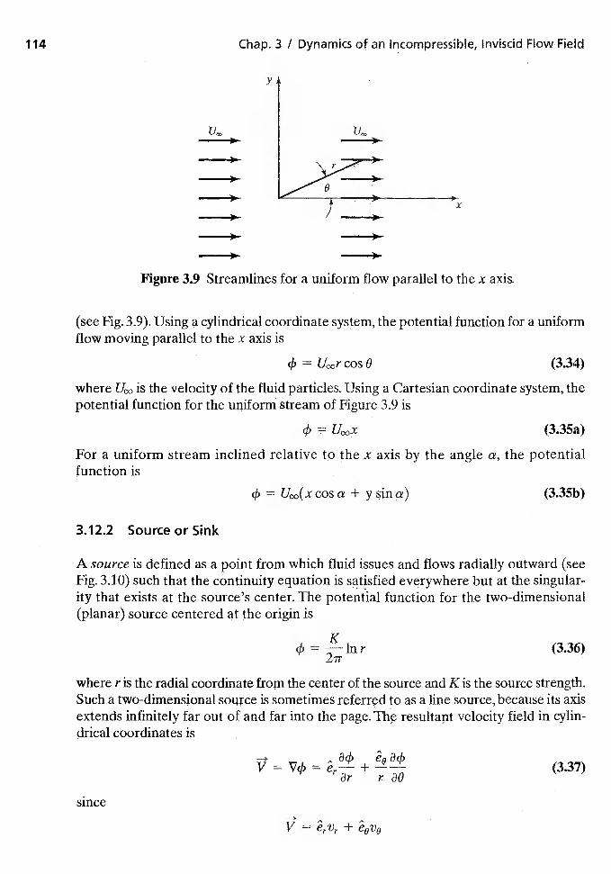
Chap. 3 I Dynamics of an Incompressible, Inviscid Flow Field
y
Figure 3.9 Streamlines for a uniform flow parallel to the x axis.
(see Fig. 3.9). Using a cylindrical coordinate system, the potential function for a uniformflow moving parallel to the x axis is
4) cos 0 (3.34)
where is the velocity of the fluid particles. Using a Cartesian coordinate system, thepotential function for the uiiiforrn stream of Figure 3.9 is
4) (335a)
For a uniform stream inclined relative to the x axis by the angle a, the potentialfunction is
4) = cos a + y sin a) (3.35b)
3.12.2 Source or Sink
A source is defined as a point from which fluid issues and flows radially outward (seeFig. 3.10) such that the continuity equation is satisfied everywhere but at the singular-ity that exists at the source's center. The potential function for the two-dimensional(planar) source centered at the origin is
4) = (336)2ir
where r is the radial coordinate from the center of the source and K is the source strength.Such a two-dimensional souTce is sometimes referred to as a line source, because its axisextends infinitely far out of and far into the page. The velocity field in cylin-drical coordinates is
V = + (3.37)ar r30
since
V ervr + eove
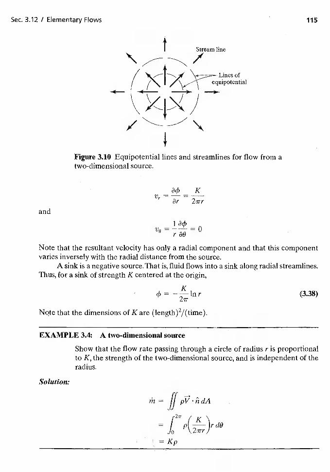
Sec. 312 I Elementary Flows 115
t Stream line/
Figure 310 Equipotential lines and streamlines for flow from atwo-dimensional source.
K
and
r öO
Note that the resultant velocity has only a radial component and that this componentvaries inversely with the radial distance from the source.
A sink is a negative source. That is, fluid flows into a sink along radial streamlines.Thus, for a sink of strength K centered at the origin,
4> = (3.38)2'n-
Note that the dimensions of K are (length)2/(time).
EXAMPLE 3.4: A two-dimensional source
Show that the flow rate passing through a circle of radius r is proportionalto K, the strength of the two-dimensional source, and is independent of theradius.
Solution:
th
/ KI p(—)rdo
Jo \271rJ
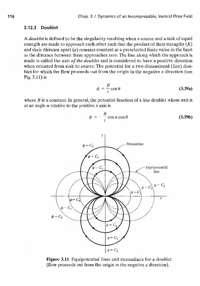
3.123 Doublet
Chap. 3 / Dynamics of an Incompressible, Inviscid Flow Field
A doublet is defined to be the singularity resulting when a source and a sink of equalstrength are made to approach each other such that the product of their strengths (K)and their distance apart (a) remains constant at a preselected finite value in the limitas the distance between them approaches zero. The line along which the approach ismade is called the axis of the doublet and is considered to have a positive directionwhen oriented from sink to source. The potential for a two-dimensional (line) dou-blet for which the flow proceeds out from the origin in the negative x direction (seeFig. 3.11) is
B4' = —cosO
r(3.39a)
where B is a constant. In general, the potential function of a line doublet whose axis isat an angle a relative to the positive x axis is
Figure 3.11 Equipotential lines and streamlines for a doublet(flow proceeds out from the origin in the negative x direction).
(3.39b)B
4, = ——cosacosOr
y
'I' = C3 Streamline
= C3
= C6
x
= C6
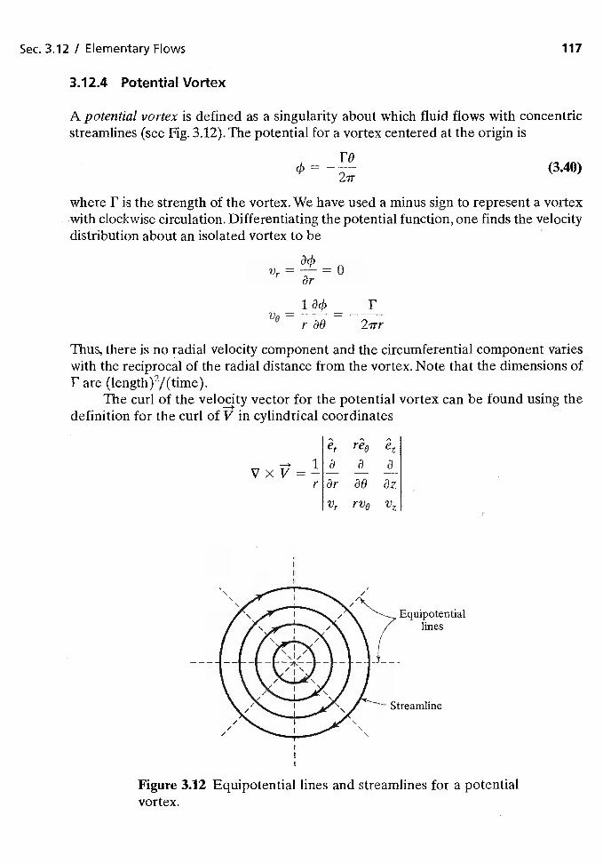
Sec. 3.12 I Elementary Flows 117
3.12.4 Potential Vortex
A potential vortex is defined as a singularity about which fluid flows with concentricstreamlines (see Fig. 3.12). The potential for a vortex centered at the origin is
= (3.40)2ir
where F is the strength of the vortex. We have used a minus sign to represent a vortexwith clockwise circulation. Differentiating the potential function, one finds the velocitydistribution about an isolated vortex to be
Vr — 03r
134" F
Thus, there is no radial velocity component and the circumferential component varieswith the reciprocal of the radial distance from the vortex. Note that the dimensions ofF are (length)2/(time).
The curl of the velocity vector for the potential vortex can be found using thedefinition for the curl of V in cylindrical coordinates
VxV=——r 9r
VT
Figure 3.12 Equipotential lines and streamlines for a potentialvortex.
a a
ao az
rv0 Vz
Equipotentiallines
Streamline
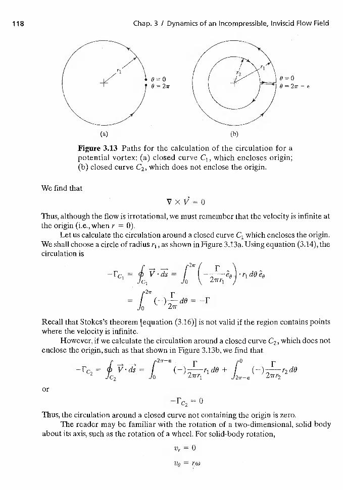
Chap. 3 / Dynamics of an Incompressible, Iriviscid Flow Field
9=0
Figure 3.13 Paths for the calculation of the circulation for apotential vortex: (a) closed curve C1, which encloses origin;(b) closed curve C2, which does not enclose the origin.
We find that
vxV=oThus, although the flow is irrotational, we must remember that the velocity is infinite atthe origin (i.e., when r = 0).
Let us calculate the circulation around a closed curve C1 which encloses the origin.We shall choose a circle of radius r1, as shown in Figure 3.13a. Using equation (3.14), thecirculation is
= = I I r1d0e0C1 Jo \ j
= I (—)—dO = —I'Jo 2ir
Recall that Stokes's theorem [equation (3.16)1 is not valid if the region contains pointswhere the velocity is infinite.
However, if we calculate the circulation around a closed curve C2, which does notenclose the origin, such as that shown in Figure 3.13b, we find that
2ir—€ 0
c2 o 2irr1 27r—E 2iir2
or
= 0
Thus, the circulation around a closed curve not containing the origin is zero.The reader may be familiar with the rotation of a two-dimensional, solid body
about its axis, such as the rotation of a wheel. For solid-body rotation,
VI = 0
V6 = rw
(a) (b)
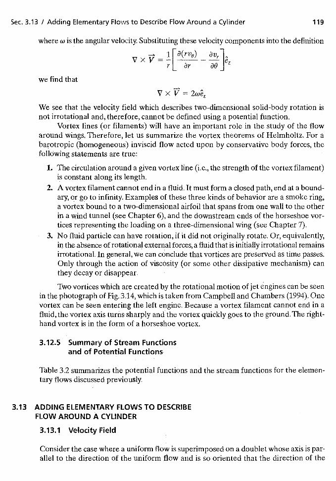
Sec. 3.13 / Adding Elementary Flows to Describe Flow Around a Cylinder 119
where is the angular velocity. Substituting these velocity components into the definition
rL 3rwe find that
We see that the velocity field which describes two-dimensional solid-body rotation isnot irrotational and, therefore, cannot be defined using a potential function.
Vortex lines (or filaments) will have an important role in the study of the flowaround wings. Therefore, let us summarize the vortex theorems of Helmholtz. For abarotropic (homogeneous) inviscid flow acted upon by conservative body forces, thefollowing statements are true:
1. The circulation around a given vortex line (i.e., the strength of the vortex filament)is constant along its length.
2. A vortex filament cannot end in a fluid. It must form a closed path, end at a bound-ary, or go to infinity. Examples of these three kinds of behavior are a smoke ring,a vortex bound to a two-dimensional airfoil that spans from one wall to the otherin a wind tunnel (see Chapter 6), and the downstream ends of the horseshoe vor-tices representing the loading on a three-dimensional wing (see Chapter 7).
3. No fluid particle can have rotation, if it did not originally rotate. Or, equivalently,in the absence of rotational external forces, a fluid that is initially irrotational remainsirrotational. In general, we can conclude that vortices are preserved as time passes.Only through the action of viscosity (or some other dissipative mechanism) canthey decay or disappear.
Two vortices which are created by the rotational motion of jet engines can be seenin the photograph of Fig. 3.14, which is taken from Campbell and Chambers (1994). Onevortex can be seen entering the left engine. Because a vortex filament cannot end in afluid, the vortex axis turns sharply and the vortex quickly goes to the ground. The right-hand vortex is in the form of a horseshoe vortex.
3.12.5 Summary of Stream Functionsand of Potential Functions
Table 3.2 summarizes the potential functions and the stream functions for the elemen-tary flows discussed previously.
3.13 ADDING ELEMENTARY FLOWS TO DESCRIBEFLOW AROUND A CYLINDER
3.13.1 Velocity Field
Consider the case where a uniform flow is superimposed on a doublet whose axis is par-allel to the direction of the uniform flow and is so oriented that the direction of the
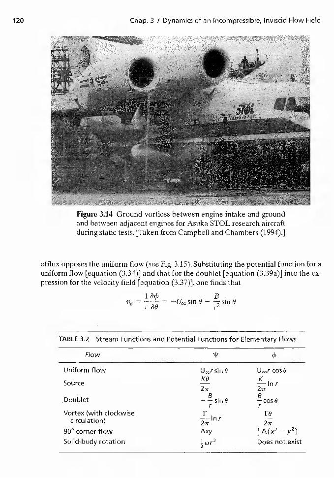
120 Chap. 3 / Dynamics of an Incompressible, Inviscid Flow Field
Figure 3.14 Ground vortices between engine intake and groundand between adjacent engines for Asuka STOL research aircraftduring static tests. [Taken from Campbell and Chambers (1994).]
efflux opposes the uniform flow (see Fig. 3.15). Substituting the potential function for auniform flow [equation (3.34)] and that for the doublet [equation (3.39a)] into the ex-pression for the velocity field [equation (3.37)], one finds that
= = —
TABLE 3.2 Stream Functions and Potential Functions for Elementary Flows
Flow 4
Uniform flow
Source
Doublet
Vortex (with clockwisecirculation)
90°cornerflowSolid-body rotation
sin 0KO
2ir
F
Axy
lwr2
cosO
K—mr2w
FO
—i—:
Does not exist
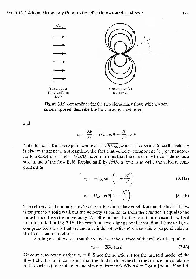
Sec. 113 I Adding Elementary Flows to Describe Flow Around a Cylinder 121
U0.
Streamlinesfor a uniform
flow
Figure 3.15 Streamlines for the two elementary flows which, whensuperimposed, describe the flow around a cylinder.
and
Bv, = — = —
0r r
Note that 0 at every point where r = which is a constant. Since the velocityis always tangent to a streamline, the fact that velocity component (vt) perpendicu-lar to a circle of r = R is zero means that the circle may be considered as astreamline of the flow field. Replacing B by R2UcYJ allows us to write the velocity com-ponents as
R2V0 = sin
+(3.41a)
7yr = cos o( 1
}(3.41b)
\\ TJThe velocity field not only satisfies the surface boundary condition that the inviscid flowis tangent to a solid wall, but the velocity at points far from the cylinder is equal to theundisturbed free-stream velocity Streamlines for the resultant inviscid flow fieldare illustrated in Fig. 3.16. The resultant two-dimensional, irrotational (inviscid), in-compressible flow is that around a cylinder of radius R whose, axis is perpendicular tothe free-stream direction.
Setting r = R, we see that the velocity at the surface of the cylinder is equal to
v0 = sin 0 (3.42)
Of course, as noted earlier, = 0. Since the solution is for the inviscid model of theflow field, it is not inconsistent that the fluid particles next to the surface move relativeto the surface (i.e., violate the no-slip requirement). When B = 0 or ir (points B and A,
Streamlines fora doublet
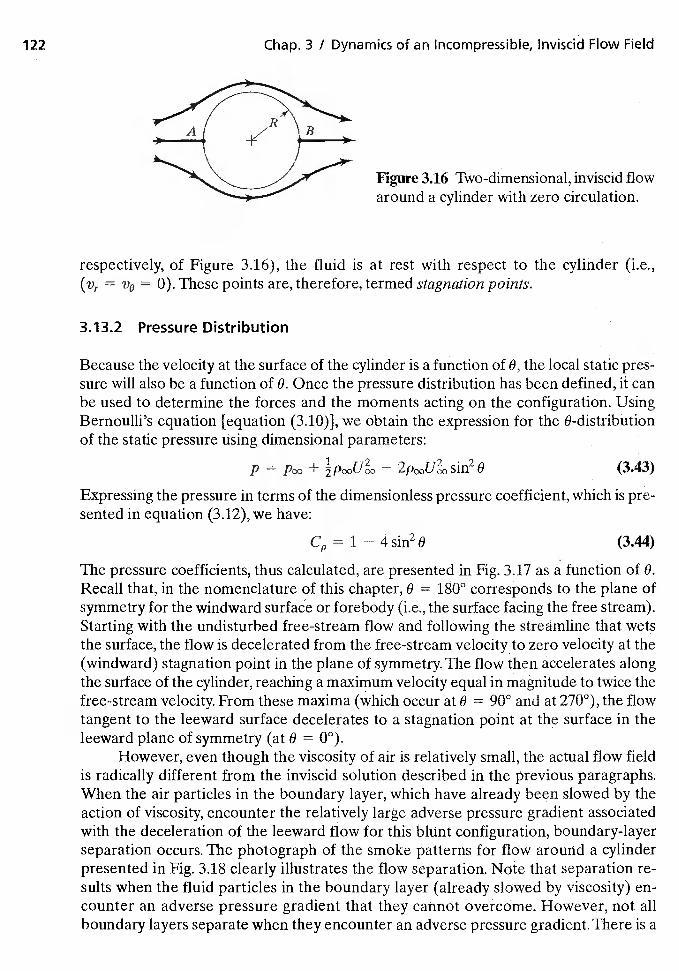
122 Chap. 3 / Dynamics of an Incompressible, Inviscid Flow Field
Figure 3.16 Two-dimensional, inviscid flowaround a cylinder with zero circulation.
respectively, of Figure 3.16), the fluid is at rest with respect to the cylinder (i.e.,(Vr = V0 = 0). These points are, therefore, termed stagnation points.
3.13.2 Pressure Distribution
Because the velocity at the surface of the cylinder is a function of 0, the local static pres-sure will also be a function of 8. Once the pressure distribution has been defined, it canbe used to determine the forces and the moments acting on the configuration. UsingBernoulli's equation [equation (3.10)], we obtain the expression for the 0-distributionof the static pressure using dimensional parameters:
p = + — sin2 0 (3.43)
Expressing the pressure in terms of the dimensionless pressure coefficient, which is pre-sented in equation (3.12), we have:
C,L, 1 — 4 sin2 0 (3.44)
The pressure coefficients, thus calculated, are presented in Fig. 3.17 as a function of 0.Recall that, in the nomenclature of this chapter, 0 = 180° corresponds to the plane ofsymmetry for the windward surface or forebody (i.e., the surface facing the free stream).Starting with the undisturbed free-stream flow and following the streamline that wetsthe surface, the flow is decelerated from the free-stream velocity to zero velocity at the(windward) stagnation point in the plane of symmetry. The flow then accelerates alongthe surface of the cylinder, reaching a maximum velocity equal in magnitude to twice thefree-stream velocity. From these maxima (which occur at 0 = 90° and at 270°), the flowtangent to the leeward surface decelerates to a stagnation point at the surface in theleeward plane of symmetry (at 8 = 0°).
However, even though the viscosity of air is relatively small, the actual flow fieldis radically different from the inviscid solution described in the previous paragraphs.When the air particles in the boundary layer, which have already been slowed by theaction of viscosity, encounter the relatively large adverse pressure gradient associatedwith the deceleration of the leeward flow for this blunt configuration, boundary-layerseparation occurs. The photograph of the smoke patterns for flow around a cylinderpresented in Fig. 3.18 clearly illustrates the flow separation. Note that separation re-suits when the fluid particles in the boundary layer (already slowed by viscosity) en-counter an adverse pressure gradient that they cannot overcome. However, not allboundary layers separate when they encounter an adverse pressure gradient. There is a
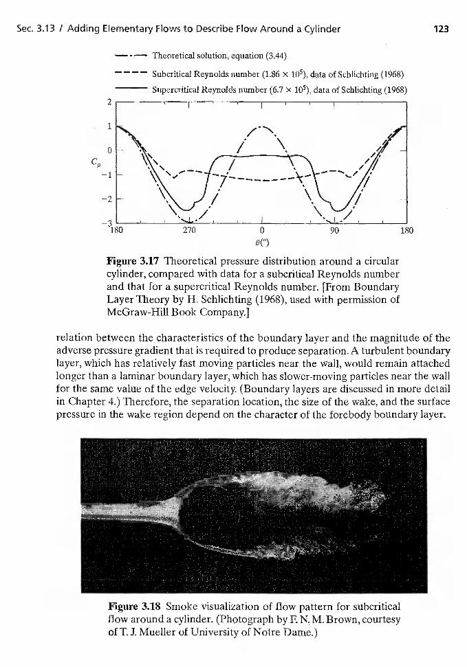
Sec. 3.13 / Adding Elementary Flows to Describe Flow Around a Cylinder 123
cp
2
1
0
—1
—2
— - — Theoretical solution, equation (3.44)
— — — — Subcritical Reynolds number (1.86 X data of Schlichting (1968)
Supercritical Reynolds number (6.7 x data of Schlichting (1968)
Figure 3.17 Theoretical pressure distribution around a circularcylinder, compared with data for a subcritical Reynolds numberand that for a supercritical Reynolds number. [From BoundaryLayer Theory by H. Schlichting (1968), used with permission ofMcGraw-Hill Book Company.]
relation between the characteristics of the boundary layer and the magnitude of theadverse pressure gradient that is required to produce separation. A turbulent boundarylayer, which has relatively fast moving particles near the wall, would remain attachedlonger than a laminar boundary layer, which has slower-moving particles near the wallfor the same value of the edge velocity. (Boundary layers are discussed in more detailin Chapter 4.) Therefore, the separation location, the size of the wake, and the surfacepressure in the wake region depend on the character of the forebody boundary layer.
Figure 3.18 Smoke visualization of flow pattern for subcriticalflow around a cylinder. (Photograph by F. N. M. Brown, courtesyofT. J. Mueller of University of Notre Dame.)
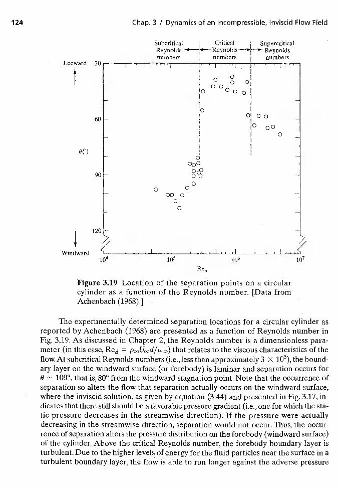
124 Chap. 3 / Dynamics of an Incompressible, Inviscid Flow Field
Subcritical Critical SupercriticalReynolds ( 4 Reynolds ) Reynoldsnumbers numbers numbers
30I i
t
60- I 0100I 10 00
0
0
0
00
00
120
1I I
106
Red
Figure 3.19 Location of the separation points on a circularcylinder as a function of the Reynolds number. [Data fromAchenbach (1968).]
The experimentally determined separation locations for a circular cylinder asreported by Achenbach (1968) are presented as a function of Reynolds number inFig. 3.19. As discussed in Chapter 2, the Reynolds number is a dimensionless para-meter (in this case, Red = that relates to the viscous characteristics of theflow. At subcritical Reynolds numbers (i.e., less than approximately 3 x the bound-ary layer on the windward surface (or forebody) is laminar and separation occurs foro 1000, that is, 800 from the windward stagnation point. Note that the occurrence ofseparation so alters the flow that separation actually occurs on the windward surface,where the inviscid solution, as given by equation (3.44) and presented in Fig. 3.17, in-dicates that there still should be a favorable pressure gradient (i.e., one for which the sta-tic pressure decreases in the streamwise direction). If the pressure were actuallydecreasing in the streamwise direction, separation would not occur. Thus, the occur-rence of separation alters the pressure distribution on the forebody (windward surface)of the cylinder. Above the critical Reynolds number, the forebody boundary layer isturbulent. Due to the higher levels of energy for the fluid particles near the surface in aturbulent boundary layer, the flow is able to run longer against the adverse pressure
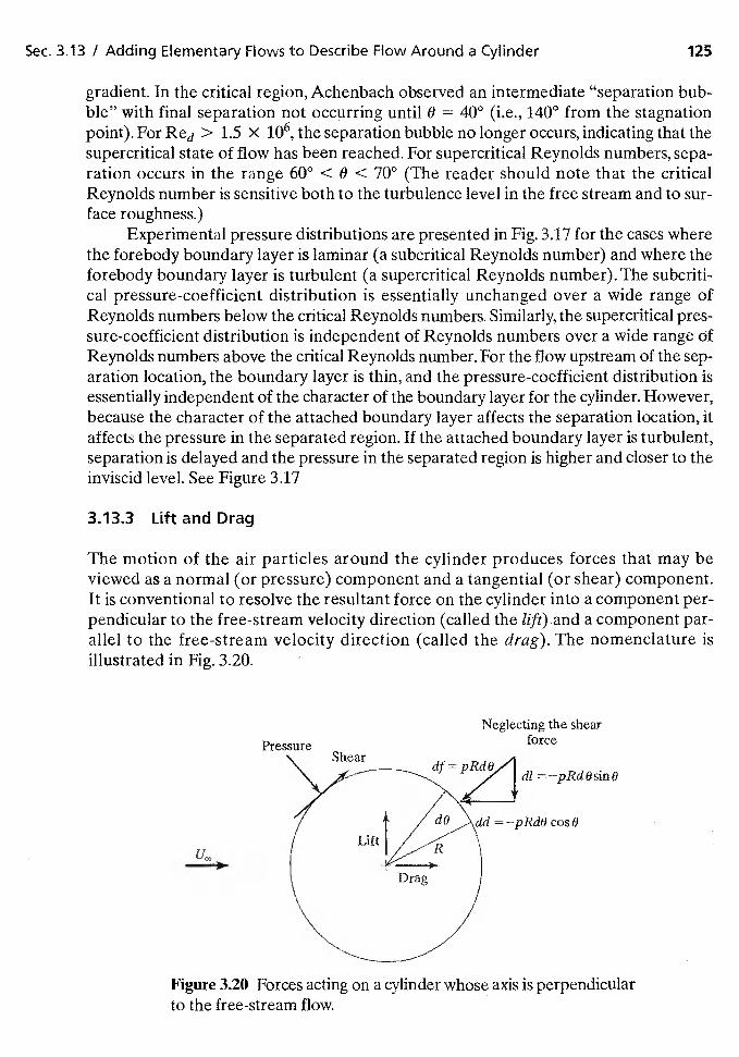
Sec. 3.13 / Adding Elementary Flows to Describe Flow Around a Cylinder 125
gradient. In the critical region, Achenbach observed an intermediate "separation bub-ble" with final separation not occurring until 8 = 400 (i.e., 140° from the stagnationpoint). For Red> 1.5 x 10⁶, the separation bubble no longer occurs, indicating that thesupercritical state of flow has been reached. For supercritical Reynolds numbers, sepa-ration occurs in the range 60° < 0 < 70° (The reader should note that the criticalReynolds number is sensitive both to the turbulence level in the free stream and to sur-face roughness.)
Experimental pressure distributions are presented in Fig. 3.17 for the cases wherethe forebody boundary layer is laminar (a subcritical Reynolds number) and where theforebody boundary layer is turbulent (a supercritical Reynolds number). The subcriti-cal pressure-coefficient distribution is essentially unchanged over a wide range ofReynolds numbers below the critical Reynolds numbers. Similarly, the supercritical pres-sure-coefficient distribution is independent of Reynolds numbers over a wide range OfReynolds numbers above the critical Reynolds number. For the flow upstream of the sep-aration location, the boundary layer is thin, and the pressure-coefficient distribution isessentially independent of the character of the boundary layer for the cylinder. However,because the character of the attached boundary layer affects the separation location, itaffects the pressure in the separated region. If the attached boundary layer is turbulent,separation is delayed and the pressure in the separated region is higher and closer to theinviscid level. See Figure 3.17
3.13.3 Lift and Drag
The motion of the air particles around the cylinder produces forces that may beviewed as a normal (or pressure) component and a tangential (or shear) component.It is conventional to resolve the resultant force on the cylinder into a component per-pendicular to the free-stream velocity direction (called the lift) and a component par-allel to the free-stream velocity direction (called the drag). The nomenclature isillustrated in Fig. 3.20.
Neglecting the shearforce
dl —pRdOsinO
=—pRdO cosO
U00
Figure 3.20 Forces acting on a cylinder whose axis is perpendicularto the free-stream flow.
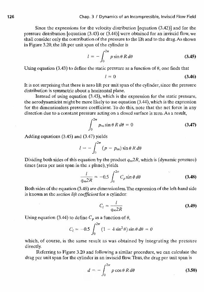
126 Chap. 3 I Dynamics of an Incompressible, Inviscid Flow Field
Since the expressions for the velocity distribution [equation (3.42)] and for thepressure distribution [equation (3.43). or (3.44)] were obtained for an inviscid flow, weshall consider only the contribution of the pressure to the lift and to the drag. As shownin Figure 3.20, the lift per Unit span of the cylinder is
p2ir
1 = — I p sin 6 R dO (345)Jo
Using equation (3.43) to define the static pressure as a function of 0, one finds that
/ = 0 (3.46)
It is not surprising that there is zero lift per unit span of the cylinder, since the pressuredistribution is symmetric about a horizontal plane.
Instead of using equation (3.43), which is the expression for the static pressure,the aerodynamicist might be more likely to use equation (3.44), which is the expressionfor the dimensionless pressure coefficient. To do this, note that the net force in anydirection due to a constant pressure acting on a closed surface is zero. As a result,
p2w
I sin 0 R dO 0 (3.47)Jo
Adding equations (3.45) and (3.47) yieldsp21T
1 = — I —
Jo
Dividing both sides of this equation by the product which is (dynamic pressure)times (area per unit span in the x plane), yields
ip2ir
—0.5 / sin 0 dO (3.48)Jo
Both sides of the equation (3.48) are dimensionless. The expression of the left-hand sideis known as the section lift coefficient for a cylinder:
C1=
(349)
Using equation (3.44) to define C,, as a function of 0,p2w
—0.5 I (1 — 4 sin2 6) sin 0 dO = 0Jo
which, of course, is the same result as was obtained by integrating the pressuredirectly.
Referring to Figure 3.20 and following a similar procedure, we can calculate thedrag per unit span for the cylinder in an inviscid flow. Thus, the drag per unit span is
d — / p cos 0 R dO (3.50)Jo
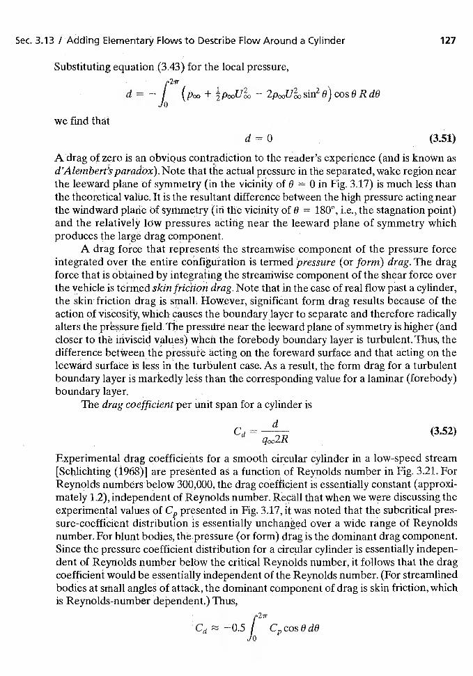
Sec. 3.13 / Adding Elementary Flows to Describe Flow Around a Cylinder 127
Substituting equation (3.43) for the local pressure,
d =—f + — sin2 o) cos 0 R dO
we find that
d=0 (3.51)
A drag of zero is an obvious contradiction to the reader's experience (and is known asd'Alembert'sparadóx). Note that the actual pressure in the separated, wake region nearthe leeward plane of symmetry (in the vicinity of 0 = 0 in Fig. 3.17) is much less thanthetheoretical value. It is the resultant difference between the high pressure acting nearthe windward plane of sythmetry (in the vicinity of 0 = 1800, i.e., the stagnation point)and the relatively 10w pressuresacthig near the leeward plane of symmetry whichproduces the large drag component.
A drag force that represents the streamwise component of the pressure forceintegrated over the entire configuration is termed pressure (or form) drag. The dragforce that is obtained by integraiing the streamwise component of the shear force overthe vehicle is termed skin friction drag. Note that in the case of real flow past a cylinder,the friction drag is small; However, significant form drag results because of theaction of viscosity, which causes the boundary layer to separate and therefore radicallyalters the pressure field. The pressure near the leeward plane of symmetry is higher (andcloser to the inviscid values) when the forebody boundary layer is turbulent. Thus, thedifference betiveen the on the foreward surface and that acting on theleeward surface is less turbulent case. As a result, the form drag for a turbulentboundary layer is markedly less than the corresponding value for a laminar (forebody)boundary layer.
The drag coefficient per unit span for a cylinder is
Cd= d
(3.52)
Experimental drag coefficients for a smooth circular cylinder in a low-speed stream[Schlichting (1968)] are presented as a function of Reynolds number in Fig. 3.21. ForReynolds numbers below 300,000, the drag coefficient is essentially constant (approxi-mately 1.2), independent of Reynolds number. Recall that when we were discussing theexperimental values of presented in Fig. 3.17, it was noted that the subcritical pres-sure-coefficient distribution is essentially unchanged over a wide range of Reynoldsnumber. For blunt bodies, the pressure (or form) drag is the dominant drag component.Since the pressure coefficient distribution for a circular cylinder is essentially indepen-dent of Reynolds number belOw the critical Reynolds number, it follows that the dragcoefficient would be essentially independent of the Reynolds number. (For streamlinedbodies at small angles of attaék, the dominant component of drag is skin friction, whichis Reynolds-number dependent.) Thus,
Cd
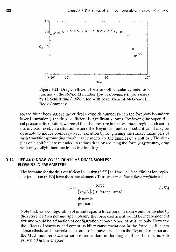
128 Chap. 3 / Dynamics of an Incompressible, inviscid Flow Field
2.0 I
1.0 000 000c000 00000 00000dD
0
Cd 0.5 -0
0000
tilt) II I I I I
4 x 10⁶
ReD
Figure 3.21 Drag coefficient for a smooth circular cylinder as afunction of the Reynolds number. [From Boundary Layer Theoryby H. Schlichting (1968), used with permission of McGraw-HillBook Company.]
for the blunt body. Above the critical Reynolds number (when the forebody boundarylayer is turbulent), the drag coefficient is significantly lower. Reviewing the supercriti-cal pressure distribution, we recall that the pressure in the separated region is closer tothe inviscid level. In a situation where the Reynolds number is subcritical, it may bedesirable to induce boundary-layer transition by roughening the surface. Examples ofsuch transition-promoting roughness elements are the dimples on a golf ball. The dim-ples on a golf ball are intended to reduce drag by reducing the form (or,pressure) dragwith only a slight increase in the friction drag.
3.14 LiFT AND DRAG COEFFiCIENTS AS DIMENSiONLESSFLOW-FIELD PARAMETERS
The formulas for the drag coefficient [equation (3.52)] and for the lift coefficient for a cylin-der [equation (3.49)] have the same elements. Thus, we can define a force coefficient as
CFforce
(353)area)
dynamicpressure
Note that, for a configuration of infinite span, a force per unit span would be divided bythe reference area per unit span. Ideally, the force coefficient would be independent ofsize and would be a function of configuration geometry and of attitude only. However,the effects of viscosity and compressibility cause variations in the force coefficients.These effects can be correlated in terms of parameters, such as the Reynolds number andthe Mach number. Such variations are evident in the drag coefficient measurementspresented in this chapter.
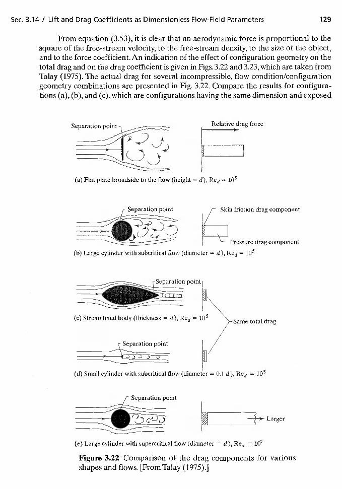
Sec. 3.14 / Lift and Drag Coefficients as Dimensionless Flow-Field Parameters 129
From equation (3.53), it is clear that an aerodynamic force is proportional to thesquare of the free-stream velocity, to the free-stream density, to the size of the object,and to the force coefficient. An indication of the effect of configuration geometry on thetotal drag and on the drag coefficient is given in Figs. 3.22 and 3.23, which are taken fromTalay (1975). The actual drag for several incompressible, flow condition/configurationgeometry combinations are presented in Fig. 3.22. Compare the results for configura-tions (a), (b), and (c), which are configurations having the same dimension and exposed
Relative drag force
,,r Separation point
(b) Large cylinder with subcritical flow (diameter = d), Rea =
(e) Large cylinder with supercritical flow (diameter = d), Red =
Figure 3.22 Comparison of the drag components for variousshapes and flows. [From Talay (1975).]
Separation point
(a) Flat plate broadside to the flow (height d), Red = i05
Skin friction drag component
Pressure drag component
point
(c) Streamlined body (thickness = d), Re1 = Same total drag
(ci) Small cylinder with subcritical flow (diameter = d), Red = i05
Separation point
Separation point
Larger
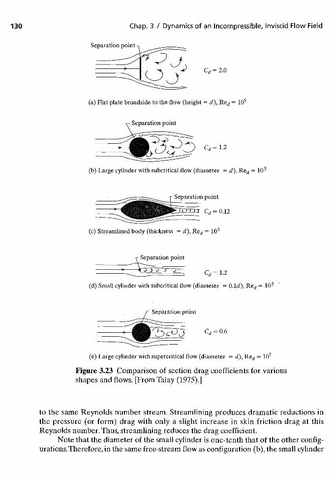
130 Chap. 3 / Dynamics of an Incompressible, Inviscid Flow Field
Cd = 2.0
(a) Flat plate broadside to the flow (height = d), Red =
\Separation point
I Cd=l.2
(b) Large cylinder with subcritical flow (diameter = d), Red
point
(c) Streamlined body (thickness = d), Red =
Separation point
Cd = 1.2
(d) Small cylinder with subcritical flow (diameter = 0.ld), Red = -
Separation point
I
(e) Large cylinder with supercritical flow (diameter = d), Red =
Figure 3.23 comparison of section drag coefficients for variousshapes and flows. [From Talay (1975).]
to the same Reynolds number stream. Streamlining produces dramatic reductions inthe pressure (or form) drag with only a slight increase in skin friction drag at thisReynolds number. Thus, streamlining reduces the drag coefficient.
Note that the diameter of the small cylinder is one-tenth that of the other config-urations. Therefore, in the same free-stream flow as configuration (b), the small cylinder
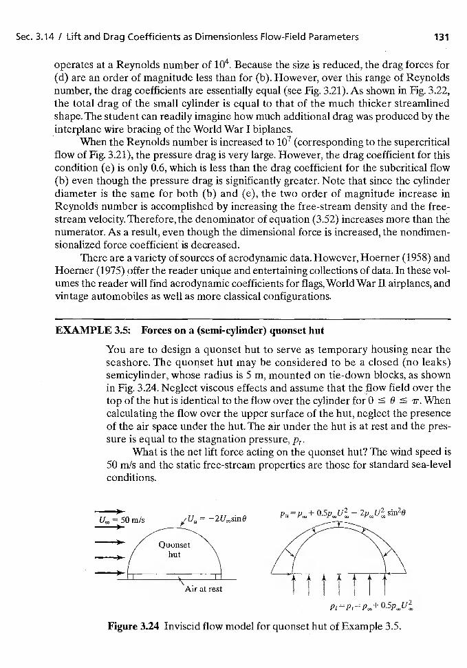
Sec. 3.14 / Lift and Drag Coefficients as Dimensionless Flow-Field Parameters 131
operates at a Reynolds number of i04. Because the size is reduced, the drag forces for(d) are an order of magnitude less than for (b). However, over this range of Reynoldsnumber, the drag coefficients are essentially equal (see Fig. 3.21). As shown in Fig. 3.22,the total drag of the small cylinder is equal to that of the much thicker streamlinedshape. The student can readily imagine how much additional drag was produced by theinterplane wire braëing of the World War I biplanes.
When the Reynolds number is increased to (corresponding to the supercriticalflow of Fig. 3.21), the pressure drag is very large. However, the drag coefficient for thiscondition (e) is only 0.6, which is less than the drag coefficient for the subcritical flow(b) even though the pressure drag is significantly greater. Note that since the cylinderdiameter is the same for both (b) and (e), the two order of magnitude increase inReynolds number is accomplished by increasing the free-stream density and the free-stream velocity. Therefore, the denominator of equation (3.52) increases more than thenumerator. As a result, even though the dimensional force is increased, the nondimen-sionalized force coefficient is decreased.
There are a variety of sources of aerodynamic data. However, Hoerner (1958) andHoerner (1975) offer the reader unique and entertaining collections of data. In these vol-umes the reader will find aerodynamic coefficients for flags, World War II airplanes, andvintage automobiles as well as more classical configurations.
EXAMPLE 3.5: Forces on a (semi-cylinder) quonset hut
You are to design a quonset hut to serve as temporary housing near theseashore. The quonset hut may be considered to be a closed (no leaks)semicylinder, whose radius is 5 m, mounted on tie-down blocks, as shownin Fig. 3.24. Neglect viscous effects and assume that the flow field over thetop of the hut is identical to the flow over the cylinder for 0 � 8 � ir. Whencalculating the flow over the upper surface of the hut, neglect the presenceof the air space under the hut. The air under the hut is at rest and the pres-sure is equal to the stagnation pressure,
What is the net lift force acting on the quonset hut? The wind speed is50 rn/s and the static free-stream properties are those for standard sea-levelconditions.
50 mIs =
hut
Air at rest
Figure 3.24 Inviscid flow model for quonset hut of Example 3.5.
I .1Pu —
Pi
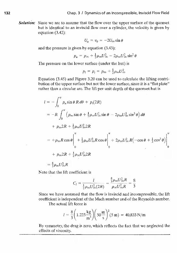
132 Chap. 3 I Dynamics of an Incompressible, Inviscid Flow Field
Solutiän: Since we are to assume that the flow over the upper surface of the quonsethut is identical to an inviscid flow over a cylinder, the velocity is given byequation (3.42):
= =
and the pressure is given by equation (3.43):
= + — sin2 0
The pressure on the lower surface (under the hut) is
Equation (3.45) and Figure 3.20 can be used to calculate the lifting contri-bution of the upper surface but not the lower surface, since it is a "flat plate"rather than a circular arc. The lift per unit depth of the quonset hut is
fir=
— I +Jo
= —R f sin 0 + sin 0 — sin3 o) dO
+ +
= + +
+
2=
Note that the lift coefficient is
i1 - — - 3
Since we have assumed that the flow is inviscid and incompressible, the liftcoefficient is independent of the Mach number and of the Reynolds number.
The actual lift force is
kg"7I = (5rn) = 40,833 N/rn
3 m 5
By symmetry, the drag is zero, which reflects the fact that we neglected theeffects of viscosity.
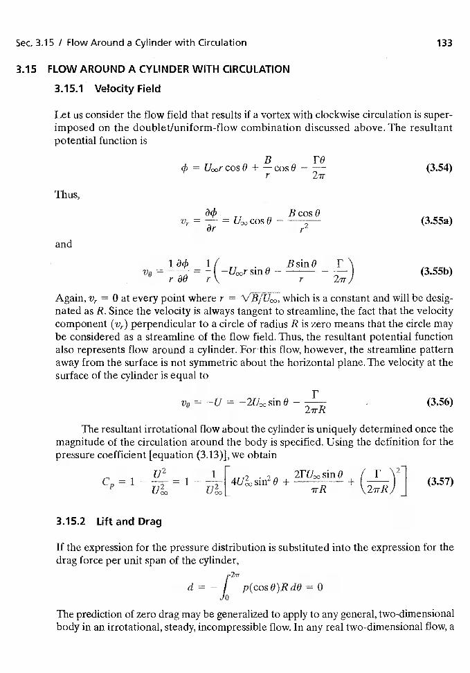
Sec. 3.15 / Flow Around a Cylinder with Circulation 133
3.15 FLOW AROUND A CYLINDER WITH CIRCULATION
3.15.1 Velocity Field
Let us consider the flow field that results if a vortex with clockwise circulation is super-imposed on the doublet/uniform-flow combination discussed above. The resultantpotential function is
= + — (3.54)r 2ir
Thus,
Bcos0Vr = cos 0
— 2(3.55a)
rand
1ä4' 11 . Bsin0 F\= = —t sin 0 — — j (3.55b)räO r 2irj
Again, = 0 at every point where r = which is a constant and will be desig-nated as R. Since the velocity is always tangent to streamline, the fact that the velocitycomponent (vi) perpendicular to a circle of radius R is zero means that the circle maybe considered as a streamline of the flow field. Thus, the resultant potential functionalso represents flow around a cylinder. Forthis flow, however, the streamline patternaway from the surface is not symmetric about the horizontal plane. The velocity at thesurface of the cylinder is equal to
v0 —U =— I'
(3.56)
The resultant irrotational flow about the cylinder is uniquely determined once themagnitude of the circulation around the body is specified. Using the definition for thepressure coefficient [equation (3.13)], we obtain
1 = 1 +0 + (2FR)2]
3.15.2 Liftand Drag
If the expression for the pressure distribution is substituted into the expression for thedrag force per unit span of the cylinder,
d I p(cos6)RdO 0Jo
The prediction of zero drag may be generalized to apply to any general, two-dimensionalbody in an irrotational, steady, incompressible flow. In any real two-dimensional flow, a
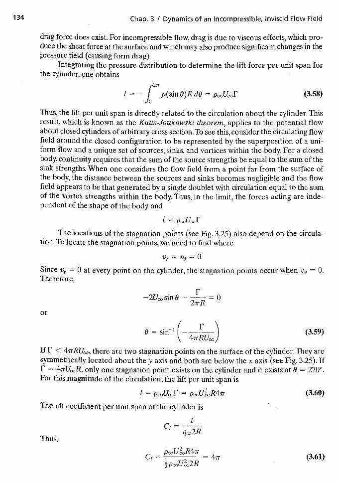
134 Chap. 3 I Dynamics of an Incompressible, Inviscid Flow Field
drag force does exist. For incompressible flow, drag is due to viscous effects, which pro-duce the shear force at the surface and which may also produce significant changes in thepressure field (causing form drag).
Integrating the pressure distribution to detennine the lift force per unit span forthe cylinder, one obtains
p2ir
1
= —Jp(sinO)RdO (3.58)
0
Thus, the lift per unit span is directly related to the circulation about the cylinder. Thisresult, which is known as the Kutta-Joukowskj theorem, applies to the potential flowabout closed cylinders of arbitrary cross section. To see this, consider the circulating flowfield around the closed configuration to be represented by the superposition of a uni-form flow and a unique set of sources, sinks, and vortices within the body. For a closedbody, continuity requires that the sum of the source strengths be equal to the sum of thesink strengths. When one considers the flow field from a point far from the surface ofthe body, the distance between the sources and sinks becomes negligible and the flowfield appears to be that generated by a single doublet with circulation equal to the sumof the vortex strengths within the body. Thus, in the limit, the forces acting are inde-pendent of the shape of the body and
I
The locatious of the stagnation points (see Fig. 3.25) also depend on the circula-tion. To locate the stagnation points, we need to find where
Vr = V0 = 0
Since Vr = 0 at every point on the cylinder, the stagnation points occur when v9 = 0.Therefore,
I, =0or
= sin1(—
(3.59)
If I' there are two stagnation points on the surface of the cylinder. They aresymmetrically located about the y axis and both are below the x axis (see Fig. 3.25). IfF = only one stagnation point exists on the cylinder and it exists at 0 2700.For this magnitude of the circulation, the lift per unit span is
7 — ir r — Yr2L — Iiooi_iooi — Poou
The lift coefficient per unit span of the cylinder is
IC1
Thus,
== (3.61)
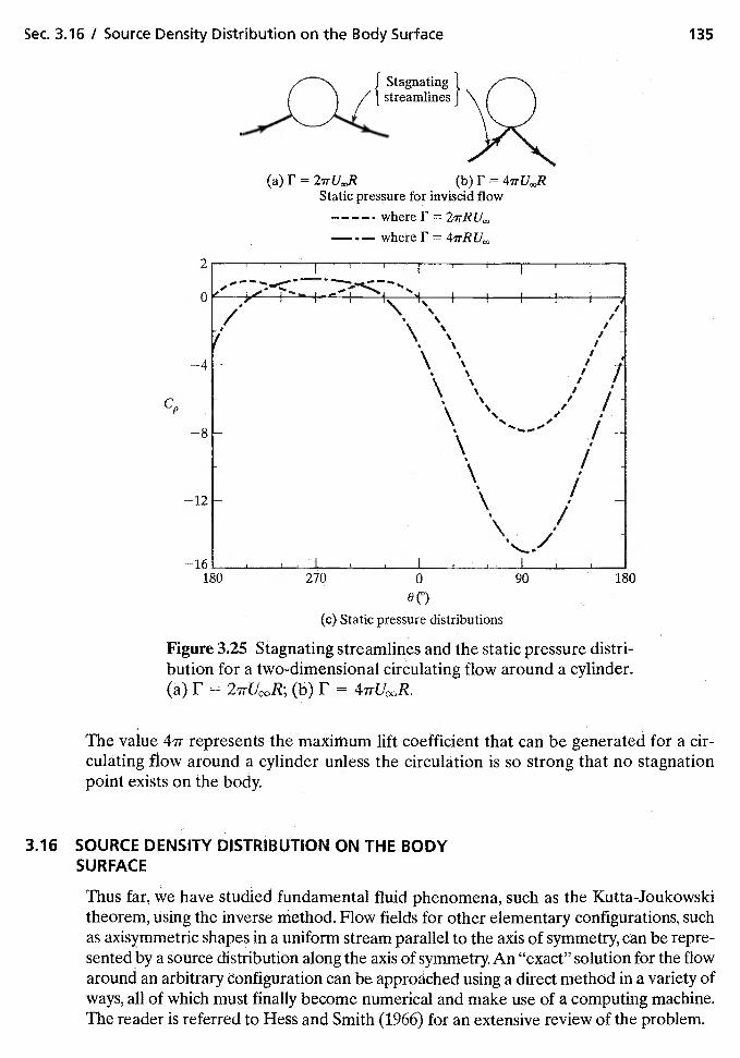
6(0)
(c) Static pressure distributions
Figure Stagnating streamlines and the static pressure distri-bution for a two-dimensional circulating flow around a cylinder.(a) F = (b) F =
The value 4ir represents the maximum lift coefficient that can be generated for a cir-culating flow around a cylinder unless the circulation is so strong that no stagnationpoint exists on the body.
3.16 SOURCE DENSITY DISTRIBUTION ON THE BODYSURFACE
Thus far, we have studied fundamental fluid phenomena, such as the Kutta-Joukowskitheorem, using the inverse method. Flow fields for other elementary configurations, suchas axisymmetric shapes in a uniform stream parallel to the axis of symmetry, can be repre-sented by a source distribution along the axis of symmetry. An "exact" solution for the flowaround an arbitrary configuration can be approached using a direct method in a variety ofways, all of which must finally become numerical and make use of a computing machine.The reader is referred to Hess and Smith (1966) for an extensive review of the problem.
Sec. 3.16 / Source Density Distribution on the Body Surface 135
(b)F=4irlJJ?Static pressure for inviscid flow
— — — —- where r = 2irR
I
,.---(1 '—I
Ce
—4 -
—8 -
—12
—16180 270
I I I
0 90 180
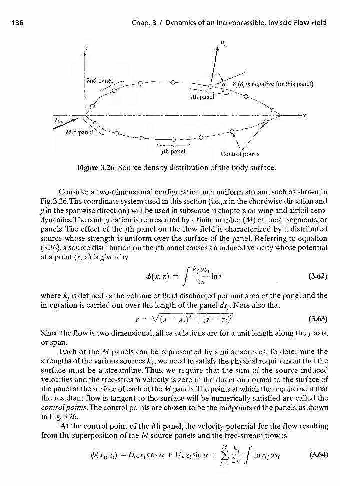
136 Chap. 3 / Dynamics of an Incompressible, lnviscid Flow Field
Figure 3.26 Source density distribution of the body surface.
Consider a two-dimensional configuration in a uniform stream, such as shown inFig. 3.26.The coordinate system used in this section (i.e., x in the chordwise direction andy in the spanwise direction) will be used in subsequent chapters on wing and airfoil aero-dynamics. The configuration is represented by a finite number (M) of linear segments, orpanels. The effect of the jth panel on the flow field is characterized by a distributedsource whose strength is uniform over the surface of the panel. Referring to equation(3.36), a source distribution on the jth panel causes an induced velocity whose potentialat a point (x, z) is given by
ç k ds14(x,z) = I mr (3.62)
where is defined as the volume of fluid discharged per unit area of the panel and theintegration is carried out over the length of the panel ds1. Note also that
r = \/(x — x1)2 + (z — z1)2 (3.63)
Since the flow is two dimensional, all calculations are for a unit length along the y axis,or span.
Each of the M panels can be represented by similar sources. To determine thestrengths of the various sources k1, we need to satisfy the physical requirement that thesurface must be a streamline. Thus, we require that the sum of the source-inducedvelocities and the free-stream velocity is zero in the direction normal to the surface ofthe panel at the surface of each of theM panels. The points at which the requirement thatthe resultant flow is tangent to the surface will be numerically satisfied are called thecontrol points.The control points are chosen to be the midpoints of the panels, as shownin Fig. 3.26.
At the control point of the ith panel, the velocity potential for the flow resultingfrom the superposition of the M source panels and the free-stream flow is
M k P= cos a + sin a +
Jin ds1 (3.64)
j=1 L.IT
zfli
for this panel)
jth panel Control points
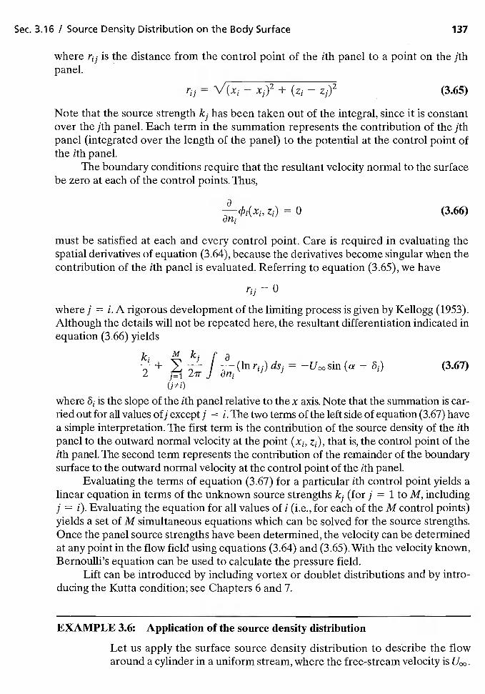
Sec. 3.16 / Source Density Distribution on the Body Surface 137
where is the distance from the control point of the ith panel to a point on the jthpanel.
= — x1)2 + (z1 — (3.65)
Note that the source strength k1 has been taken out of the integral, since it is constantover the jth panel. Each term in the summation represents the contribution of the jthpanel (integrated over the length of the panel) to the potential at the control point ofthe ith panel.
The boundary conditions require that the resultant velocity normal to the surfacebe zero at each of the control points. Thus,
= 0 (3.66)
must be satisfied at each and every control point. Care is required in evaluating thespatial derivatives of equation (3.64), because the derivatives become singular when thecontribution of the ith panel is evaluated. Referring to equation (3.65), we have
rj3 = 0
where j = i. A rigorous development of the limiting process is given by Kellogg (1953).Although the details will not be repeated here, the resultant differentiation indicated inequation (3.66) yields
/c M k1(3.67)
j=1 IT flj
where is the slope of the ith panel relative to the x axis. Note that the summation is car-ried out for all values of j except j = i. The two terms of the left side of equation (3.67) havea simple interpretation. The first term is the contribution of the source density of the ithpanel to the outward normal velocity at the point (xi, z1), that is, the control point of theith panel. The second term represents the contribution of the remainder of the boundarysurface to the outward normal velocity at the control point of the ith panel.
Evaluating the terms of equation (3.67) for a particular ith control point yields alinear equation in terms of the unknown source strengths k3 (for j = 1 to M, includingj = i). Evaluating the equation for all values of i (i.e., for each of the M control points)yields a set of M simultaneous equations which can be solved for the source strengths.Once the panel source strengths have been determined, the velocity can be determinedat any point in the flow field using equations (3.64) and (3.65). With the velocity known,Bernoulli's equation can be used to calculate the pressure field.
Lift can be introduced by including vortex or doublet distributions and by intro-ducing the Kutta condition; see Chapters 6 and 7.
EXAMPLE 3.6: Application of the source density distribution
Let us apply the surface source density distribution to describe the flowaround a cylinder in a uniform stream, where the free-stream velocity is
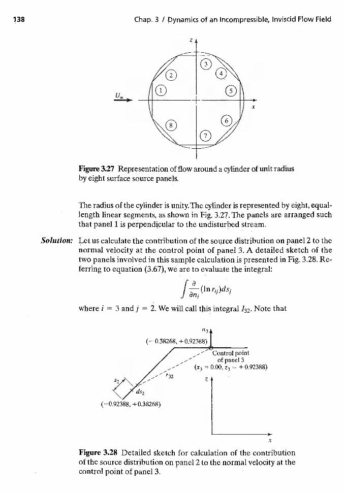
Figure 3.27 Representation of flow around a cylinder of unit radiusby eight surface source panels.
The radius of the cylinder is unity. The cylinder is represented by eight, equal-length linear segments, as shown in Fig. 3.27. The panels are arranged suchthat panel 1 is perpendicular to the undisturbed stream.
Solution: Let us calculate the contribution of the source distribution on panel 2 to thenormal velocity at the control point of panel 3. A detailed sketch of thetwo panels involved in this sample calculation is presented in Fig. 3.28. Re-ferring to equation (3.67), we are to evaluate the integral:
(in
where i 3 and j = 2. We will call this integral 132,Note that
— Control pointof panel3
(x3 0.00, z3 = ± 0.92388)
z
Figure 3.28 Detailed sketch for calculation of the contributionof the source distribution on panel 2 to the normal velocity at thecontrol point of panel 3.
138 Chap. 3 / Dynamics of an Incompressible, Inviscid Flow Field
U0.
x
fl3
(— 0.38268, + 0.92388)/ —/ ,..— r32
(—0.92388, +0.38268)
x
Sec. 316 I Source Density Distribution on the Body Surface 139
a tar32—
0n3 r32 an3
8x3 az3(x3 — x2)— + (z3 — Z2)
an3 8n3= (368)
(x3 — x2)2 + (z3 — z2)2
where x3 = 0.00 and Z3 0.92388 are the coordinates of the control pointof panel 3. Note also that
ax3 az3= 0.00, = 1.00
an3 0n3
Furthermore, for the source line represented by panel 2,
= —0.92388 + 0.70711s2
= +0.38268 + 0.70711s2
and the length of the panel is
12 = 0.76537
Combining these expressions, we obtain[0.76537 (0.92388 — 0.38268 — 0.70711s2) ds2
'32— Jo (0.92388 — 0.70711s2)2 + (0.92388 — 0.38268 — 0.70711s2)2
This equation can be rewritten0.76537 ds
'32 = 0.541202
o 1.14645 — 2.07195s2 +
J0.76537 s2as2
—0.707110 1.14645 — 2.07195s2 +
Using the integral tables to evaluate these expressions, we obtain
'32 = — 2.07195s2 +
[ — (2s2 — 2.07195\132=0.76537—0.70711' tan I[ \/0.29291 —320
Thus,
'32 = 0.3528
In a similar manner, we could calculate the contributions of source pan-els 1,4, 5,6,7, and 8 to the normal velocity at the control point of panel 3. Sub-stituting the values of these integrals into equation (3.67), we obtain a linearequation of the form
131k1 + 1321c2 + irk3 + + 133k5 + 136k6 + 137k7 + 138k8 = 0.00 (3.69)
The right-hand side is zero since a 0 and = 0.
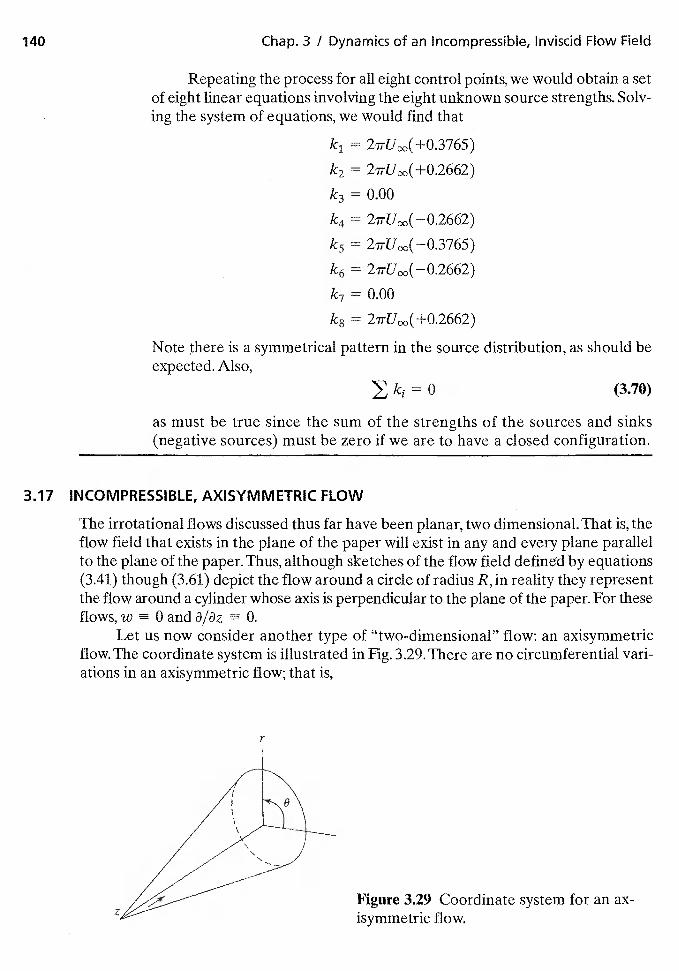
Chap. 3 / Dynamics of an Incompressible, Inviscid Flow Field
Repeating the process for all eight control points, we would obtain a setof eight linear equations involving the eight unknown source strengths. Solv-ing the system of equations, we would find that
k1 = 2ITUc,o(+0.3765)
k2 =
k3 = 0,00
k5 =
=
= 0.00
k8 =
Note there is a symmetrical pattern in the source distribution, as should beexpected. Also,
(370)
as must be true since the sum of the strengths of the sources and sinks(negative sources) must be zero if we are to have a closed configuration.
3.17 INCOMPRESSIBLE, AXISYMMETRIC FLOW
The irrotational flows discussed thus far have been planar, two dimensional. That is, theflow field that exists in the plane of the paper will exist in any and every plane parallelto the plane of the paper. Thus, although sketches of the flow field defined by equations(3.41) though depict the flow around a circle of radius R, in reality they representthe flow around a cylinder whose axis is perpendicular to the plane of the paper. For theseflows, w 0 and 3/0z 0.
Let us now consider another type of "two-dimensional" flow: an axisymmetricThe coordinate system is illustrated in Fig. 3.29. There are no circumferential vari-
ations in an axisymmetric flow; that is,
Figure 3.29 Coordinate system for an ax-isymmetric flow.
Sec. 3.17 / Incompressible, Axisymmetric Flow 141
v0—0 and
Thus, the incompressible, continuity equation becomes
—+—+—=o3r r 3z
Noting that r and z are the independent coordinates (i.e., variables), we can rewrite thisexpression as
+ = 0 (3.71)
As has been discussed, a stream function will exist for an incompressible, two-dimen-sional flow. The flow need be two dimensional only in the sense that it requires onlytwo spatial coordinates to describe the motion, The stream function that identically sat-isfies equation (3.71) is
—=rv,. and3z
Thus, in the coordinate system of Fig. 3.29,
'Or = and v = (3.72)r3z Z r3r
Note that = constant defines a stream surface.
3.17.1 Flow around a Sphere
To describe a steady, inviscid,, incompressible flow around a sphere, we will add theaxisymmetric potential functions for a uniform flow and for a point doublet. We willfirst introduce the necessary relations in spherical coordinates. For a spherical coordi-nate system,
1v,. = — v0 = , (3.73)
3r r 3w rsina 30
for an irrotational flow where V = V4. In equation (3.73), f represents the potentialfunction, and r, 0, and w represent the independent coordinates. By symmetry,
v0=0 and
The velocity potential for an axisymmetric doublet is
B4=+
where the doublet is so oriented that the source is placed upstream and the doublet axisis parallel to the uniform flow. The potential function for a uniform flow is
142 Chap. 3 / Dynamics of an Incompressible, Inviscid Flow Field
4) cos
Thus, the sum of the potential functions is
4) = +B
4'n-r
The velocity components for this potential function are
aq5 B= — 3cosw (3.75a)
aT 2irrand
B.= = — ,sinw (3.75b)r 3w
As we did when modeling the inviscid flow around a cylinder, we note that
VT = 0when
Br3 = constant = R3
Thus, if B = we can use the potential function described by equation(3.74) to describe steady, inviscid, incompressible flow around a sphere of radius R. Forthis flow,
= 1 — —i- jcosw (3.76a)rJand
_uoo(i + (3.76b)2r
On the surface of the sphere (i.e., for r = R), the resultant velocity is given by
U = 1171 = = — sin w (3.77)
The static pressure acting at any point on the sphere can be calculated using equa-tion (3.77) to represent the local velocity in Bernoulli's equation:
p = + — sin2 (0) (3.78)
Rearranging the terms, we obtain the expression for the pressure coefficient for steady,inviscid, incompressible flow around a sphere:
= I — (3.79)
Compare this expression with equation (3.44) for flow around a cylinder of infinite spanwhose axis is perpendicular to the free-stream flow:
= I — 4sin2O
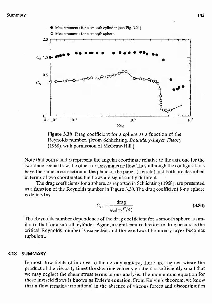
Summary 143
* Measurements for a smooth cylinder (see Fig. 3.21)
o Measurements for a smooth sphere2.0
I
•• •****•.s..Cdl.0
0.5
0.1 I
4x10³ 106
Figure 3.30 Drag coefficient for a sphere as a function of theReynolds number. [From Schlichting, Boundary-Layer Theory(1968), with permission of McGraw-HilL]
Note that both 0 and o represent the angular coordinate relative to the axis, one for thetwo-dimensional flow, the other for axisymmetric flow. Thus, although the configurationshave the same cross section in the plane of the paper (a circle) and both are describedin terms of two coordinates, the flows are significantly different.
The drag coefficients for a sphere, as reported in Schlichting (1968), are presentedas a function of the Reynolds number in Figure 3.30. The drag coefficient for a sphereis defined as
CD= drag
(3.80)/4)
The Reynolds number dependence of the drag coefficient for a smooth sphere is sim-ilar to that for a smooth cylinder. Again, a significant reduction in drag occurs as thecritical Reynolds number is exceeded and the windward boundary layer becomesturbulent.
3.18 SUMMARY
In most flow fields of interest to the aerodynamicist, there are regions where theproduct of the viscosity times the shearing velocity gradient is sufficiently small thatwe may neglect the shear stress terms in our analysis. The momentum equation forthese inviscid flows is known as Euler's equation. From Kelvin's theorem, we knowthat a flow remains irrotational in the absence of viscous forces and discontinuities
S
Red
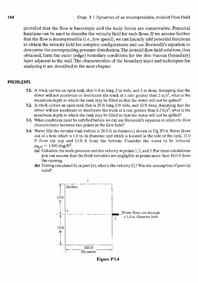
144 Chap. 3 / Dynamics of an Incompressible, Inviscid Flow Field
provided that the flow is barotropic and the body forces are conservative. Potentialfunctions can be used to describe the velocity field for such flows. If we assume furtherthat the flow is incompressible (i.e., low speed), we can linearly add potential functionsto obtain the velocity field for complex configurations and use Bernouffi's equation todetermine the corresponding pressure distribution. The inviscid flow field solutions, thusobtained, form the outer (edge) boundary conditions for the thin viscous (boundary)layer adjacent to the walLThe characteristics of the boundary layer and techniques foranalyzing it are described in the next chapter.
PROBLEMS
3.1. A truck carries an open tank, that is 6 m long, 2 m wide, and 3 m deep. Assuming that thedriver will not accelerate or decelerate the truck at a rate greater than 2 m/s2, what is themaximum depth to which the tank may be filled so that the water will not be spilled?
3.2. A truck carries an open tank that is 20 ft long, 6 ft wide, and 10 ft deep. Assuming that thedriver will not accelerate or decelerate the truck at a rate greater than 6.3 ft/s2, what is themaximum depth to which the tank may be filled so that the water will not be spilled?
3.3. What conditions must be satisfied before we can use Bernoulli's equation to relate the flowcharacteristics between two points in the flow field?
3.4. Water fills the circular tank (which is 20.0 ft in diameter) shown in Fig. P3.4. Water flowsout of a hole which is 1.0 in. in diameter and which is located in the side of the tank, 15.0ft from the top and 15.0 ft from the bottom. Consider the water to be inviscid.PH20 = 1.940 slug/ft3.(a) Calculate the static pressure and the velocity at points 1,2, and 3. For these calculations
you can assume that the fluid velocities are negligible at points more than 10.0 ft fromthe opening.
(b) Having calculated U3 in part (a), what is the velocity U1? Was the assumption of part (a)valid?
Surface
1
15.0ft
—2 - — - - - — - — - flows out through
a 1.0 in, diameter hole
110
20.0 ftDiameter
Figure P3.4
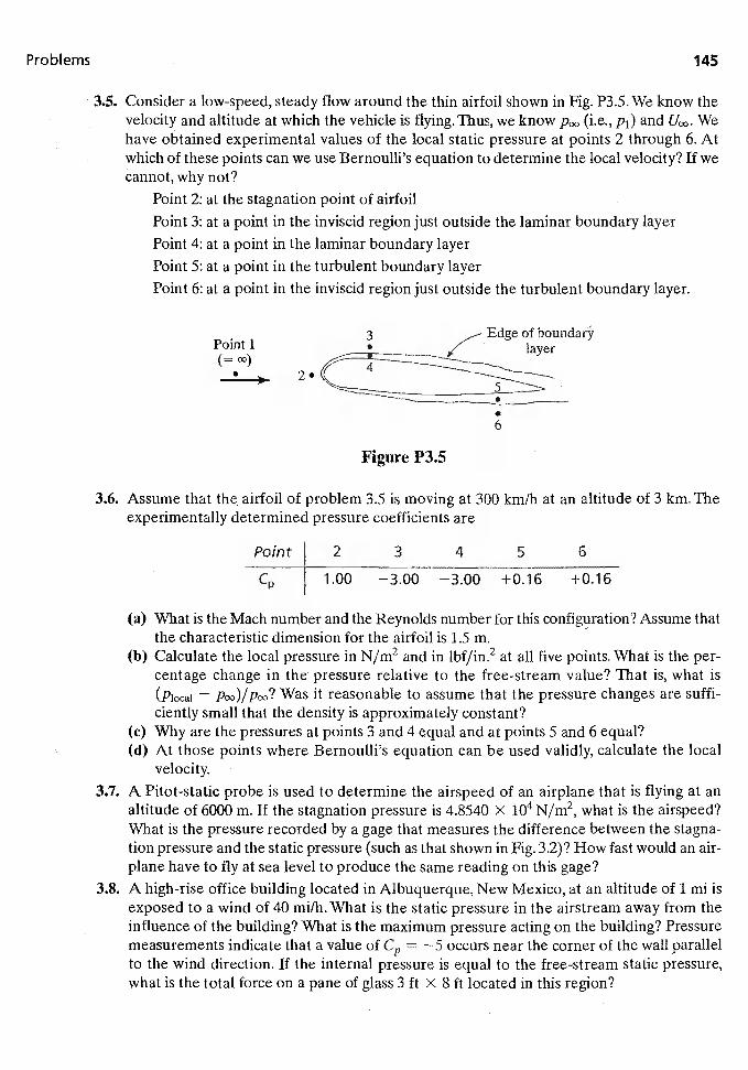
Problems 145
3.5. Consider alow-speed, steady flow around the thin airfoil shown in Fig. P35. We know thevelocity and altitude at which the vehicle is flying. Thus, we know (i.e., Pi) and Wehave obtained experimental values of the local static pressure at points 2 through 6. Atwhich of these points can we use Bernoulli's equation to determine the local velocity? If wecannot, why not?
Point 2: at the stagnation point of airfoilPoint 3: at a point in the inviscid region just outside the laminar boundary layerPoint 4: at a point in the laminar boundary layerPoint 5: at a point in the turbulent boundary layerPoint 6: at a point in the inviscid region just outside the turbulent boundary layer.
2'
of boundary
Figure P3.5
3.6. Assume that the airfoil of problem 3.5 is moving at 300 km/h at an altitude of 3 km. Theexperimentally determined pressure coefficients are
Point 2 3 4 5 6
1.00 —3.00 —3.00 +0.16 +0.16
(a) What is the Mach number and the Reynolds number for this configuration? Assume thatthe characteristic dimension for the airfoil is 1.5 rn.
(b) Calculate the local pressure in N/rn2 and in lbf/in.2 at all five points. What is the per-centage change in the pressure relative to the free-stream value? That is, what is(Piocai — Was it reasonable to assume that the pressure changes are suffi-ciently small that the density is approximately constant?
(c) Why are the pressures at points 3 and 4 equal and at points 5 and 6 equal?(ci) At those points where Bernoulli's equation can be used validly, calculate the local
velocity.
3.7. A Pitot-static probe is used to determine the airspeed of an airplane that is flying at analtitude of 6000 m. If the stagnation pressure is 4.8540 X N/rn2, what is the airspeed?What is the pressure recorded by a gage that measures the difference between the stagna-tion pressure and the static pressure (such as that shown in Fig. 3.2)? How fast would an air-plane have to fly at sea level to produce the same reading on this gage?
3.8. A high-rise office building located in Albuquerque, New Mexico, at an altitude of 1 mi isexposed to a wind of 40 mi/h. What is the static pressure in the airstream away from theinfluence of the building? What is the maximum pressure acting on the building? Pressuremeasurements indicate that a value of = —5 occurs near the corner of the wall parallelto the wind direction. If the internal pressure is equal to the free-stream static pressure,what is the total force on a pane of glass 3 ft X 8 ft located in this region?
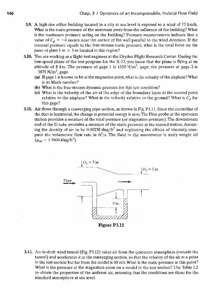
146 Chap. 3 / Dynamics of an Incompressible, Inviscid Flow Field
3.9. A high-rise office building located in a city at sea level is exposed to a wind of 75 km/h.What is the static pressure of the airstream away from the influence of the building? Whatis the maximum pressure acting on the building? Pressure measurements indicate that avalue of = —4 occurs near the corner of the wall parallel to the wind direction. If theinternal pressure equals to the free-stream static pressure, what is the total force on thepane of glass 1 m X 3 m located in this region?
3.10. You are working as a flight-test engineer at the Flight Research Center. During thelow-speed phase of the test program for the X-37, you know that the plane is flying at analtitude of 8 km. The pressure at gage 1 is 1550 N/rn2, gage; the pressure at gage 2 is—3875 N/rn2, gage.(a) If gage 1 is known to be at the stagnation point, what is the velocity of the airplane? What
is its Mach number?(b) What is the free-stream dynamic pressure for this test condition?(c) What is the velocity of the air at the edge of the boundary layer at the second point
relative to the airplane? What is the velocity relative to the ground? What is forthis gage?
3.11. Air flows through a converging pipe section, as shown in Fig. P3.11. Since the centerline ofthe duct is horizontal, the change in potential energy is zero. The Pitot probe at the upstreamstation provides a measure of the total pressure (or stagnation pressure). The downstreamend of the U-tube provides a measure of the static pressure at the second station. Assum-ing the density of air to be 0.00238 slug/ft3 and neglecting the effects of viscosity, com-pute the volumetric flow rate in ft3/s. The fluid in the manometer is unity weight oil
= 1.9404 slug/ft3).
Flow
3.12. An in-draft wind tunnel (Fig. P3J2) takes air from the quiescent atmosphere (outside thetunnel) and accelerates it in the converging section, so that the velocity of the air at a pointin the test section but far from the model is 60 rn/s. What is the static pressure at this point?What is the pressure at the stagnation point on a model in the test section? Use Table 1.2to obtain the properties of the ambient air, assuming that the conditions are those for thestandard atmosphere at sea level.
Figure P3.11
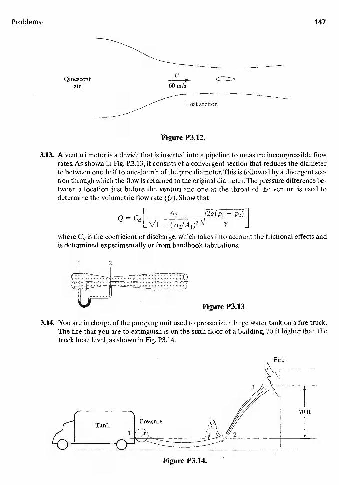
QuiescentU
68 rn/s
Figure P3.12.
3.13. A venturi meter is a device that is inserted into a pipeline to measure incompressible flowrates. As shown in Fig. P.3.13, it consists of a convergent section that reduces the diameterto between one-half to one-fourth of the pipe diameter. This is followed by a divergent sec-tion through which the flow is returned to the original diameter. The pressure difference be-tween a location just before the venturi and one at the throat of the venturi is used todetermine the volumetric flow rate (Q). Show that
— [ A2 /2g(p1 — P2)
[Vi — (AilA1)2where Cd is the coefficient of discharge, which takes into account the frictional effects andis determined experimentally or from handbook tabulations.
Figure P3.13
3.14. You are in charge of the pumping unit used to pressurize a large water tank on a fire truck.The fire that you are to extinguish is on the sixth floor of a building, 70 ft higher than thetruck hose level, as shown in Fig. P3.14.
Problems 147
air
Fire
3
Pressure
70 ft
Figure P3.14.
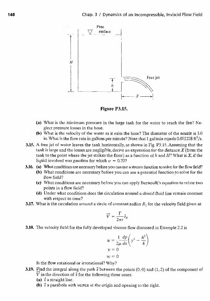
148 Chap. 3 I Dynamics of an Incompressible, Inviscid Flow Field
Freesurface
I
IF X____
Figure P3.15.
(a) What is the minimum pressure in the large tank for the water to reach the fire? Ne-glect pressure losses in the hose.
(b) What is the velocity of the water as it exits the hose? The diameter of the nozzle is 3.0in. What is the flow rate in gallons per minute? Note that 1 gallmin equals 0.002228 ft3/s.
3.15. A free jet of water leaves the tank horizontally, as shown in Fig. P3.15. Assuming that thetank is large and the losses are negligible, derive an expression for the distance X (from thetank to the point where the jet strikes the floor) as a function of h and H? What is X, if theliquid involved was gasoline for which o = 0,70?
3.16. (a) What conditions are necessary before you can use a stream function to solve for the flow field?(b) What conditions are necessary before you can use a potential function to solve for the
flow field?(c) What conditions are necessary before you can apply Bernoulli's equation to relate two
points in a flOw field?(il) Under what conditions does the circulation around a closed fluid line remain constant
with respect to time?3.17. What is the circulation around a circle of constant radius R1 for the velocity field given as
-+V = —e0
2'irr
3.18. The velocity field for the fully developed viscous flow discussed in Example 2.2 is
idp(2 h2U = y — *4v=0w = 0
Is the flow rotational or irrotational? Why?3.19. Find the integral along the path between the points (0,0) and (1,2) of the component of
V in the direction of for the following three cases:(a) a straight line.(b) a parabola with vertex at the origin and opening to the right.
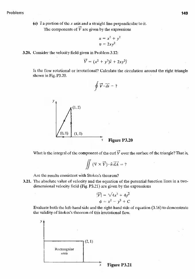
Problems 149
(c) a portion of the x axis and a straight line perpendicular to it.The components of V are given by the expressions
U = X2 + y2
v = 2xy2
3.20. Consider the velocity field given in Problem 3.12:
(x2 + y2)I + 2xy2]
Is the flow rotational or irrotational? Calculate the circulation around the right triangleshown in Fig. P3.20.
y
(1,2)
(1,0)
Figure P3.20
What is the integral of the component of the curl over the surface of the triangle? That is,
Are the results consistent with Stokes's theorem?3.21. The absolute value of velocity and the equation of the potential function lines in a two-
dimensional velocity field (Fig. P3.21) are given by the expressions
JVJ = \/4x2 + 4y2
= — y2 + cEvaluate both the left-hand side and the right-hand side of equation (3.16) to demonstratethe validity of Stokes's theorem of this irrotational flow.
y
(2, 1)
Rectangulararea
Figure P3.21
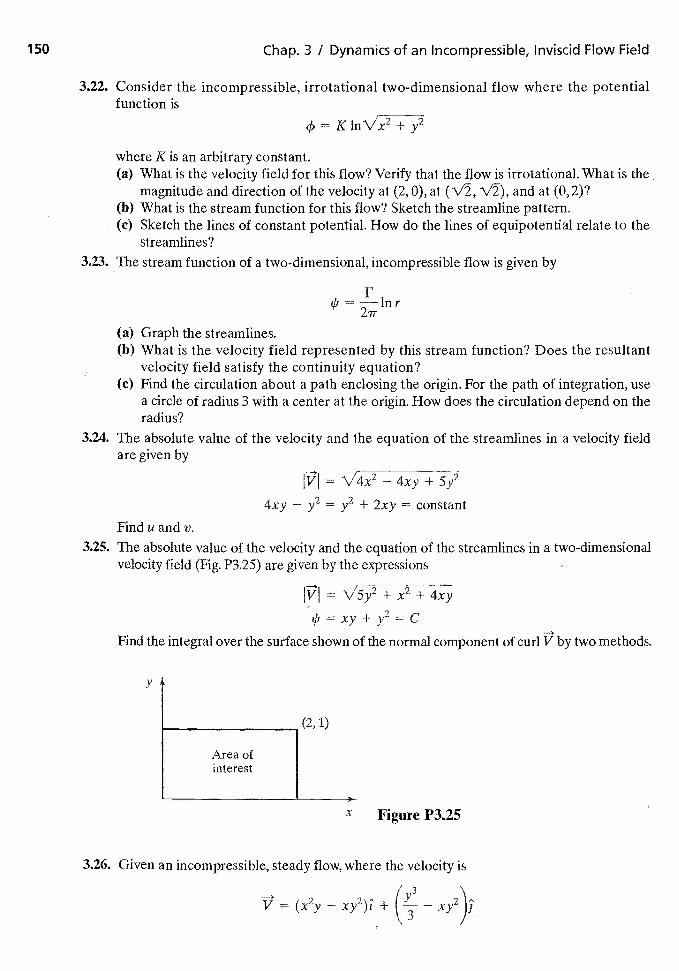
Chap. 3 / Dynamics of an Incompressible, Inviscid Flow Field
3.22. Consider the incompressible, irrotational two-dimensional flow where the potentialfunction is
=
K is an arbitrary constant.(a) What is the velocity field for this flow? Verify that the flow is irrotational. What is the
magnitude and direction of the velocity at (2,0), at and at (0,2)?(b) What is the stream function for this flow? Sketch the streamline pattern.(c) Sketch the lines of constant potential. How do the lines of equipotential relate to the
streamlines?3.23. The stream function of a two-dimensional, incompressible flow is given by
cli =
(a) Graph the streamlines.(b) What is the velocity field represented by this stream function? Does the resultant
velocity field satisfy the continuity equation?(c) Find the circulation about a path enclosing the origin. For the path of integration, use
a circle of radius 3 with a center at the origin. How does the circulation depend on theradius?
3.24. The absolute value of the velocity and the equation of the streamlines in a velocity fieldare given by
IT/I = V4x2 — 4xy + 5y2
4xy — y2 = y2 + 2xy = constant
Find uandv.3.25, The absolute value of the velocity and the equation of the streamlines in a two-dimensional
velocity field (Fig. P3.25) are given by the expressions
= + x2 + 4xy
= xy + = C
Find the integral over the surface shown of the normal component of curl by two methods.
y
(2,1)
Area ofinterest
X Figure P3.25
3.26. Given an incompressible, steady flow, where the velocity is
= - xy2)I+
—
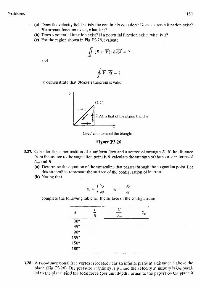
Problems
(a) Does the velocity field satisfy the continuity equation? Does a stream function exist?If a stream function exists, what is it?
(b) Does a potential function exist? If a potential function exists, what is it?(c) For the region shown in Fig. P3.26, evaluate
and
Circulation around the triangle
Figure P3,26
3.27. Consider the superposition of a uniform flow and a source of strength K. If the distancefrom the source to the stagnation point is R, calculate the strength of the source in terms of
and R.(a) Determine the equation of the streamline that passes through thestagnation point. Let
this streamline represent the surface of the configuration of interest.(b) Noting that
1
complete the following table for the surface of the configuration.
0r—R
UC'°
30°450
90°1350
1500
1800
3.28. A two-dimensional free vortex is located near an infinite plane at a distance h above theplane (Fig, P3.28). The pressure at infinity is and the velocity at infinity is paral-lel to the plane. Find the total force (per unit depth normal to the paper) on the plane if
to demonstrate that Stokes's theorem is valid.
y
(1,1)
dA is that of the planar triangle
x
V0 =ar
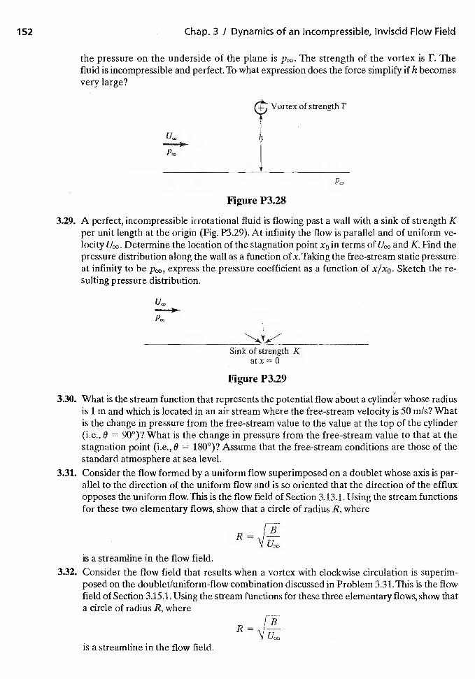
152 Chap. 3 / Dynamics of an Incompressible, Iriviscid Flow Field
the pressure on the underside of the plane is The strength of the vortex is r. Thefluid is incompressible and perfect. To what expression does the force simplify if h becomesvery large?
+ Vortex of strength I'
h
PC,,
Figure P3,28
3.29. A perfect, incompressible irrotational fluid is flowing past a wall with a sink of strength Kper unit length at the origin (Fig. P3.29). At infinity the flow is parallel and of uniform ve-locity Determine the location of the stagnation point x0 in terms of and K. Find thepressure distribution along the wall as a function of x. Taking the free-stream static pressureat infinity to be express the pressure coefficient as a function of x/xo. Sketch the re-sulting pressure distribution.
U,0
Sink of strength Katx=O
Figure P3.29
330. What is the stream function that represents the potential flow about a cylinder whose radiusis 1 m and which is located in an air stream where the free-stream velocity is 50 mIs? Whatis the change in pressure from the free-stream value to the value at the top of the cylinder(i.e., 6 = 90°)? What is the change in pressure from the free-stream value to that at thestagnation point (i.e., 0 = 180°)? Assume that the free-stream conditions are those of thestandard atmosphere at sea level.
3.31. Consider the flow formed by a uniform flow superimposed on a doublet whose axis is par-allel to the direction of the uniform flow and is so oriented that the direction of the effluxopposes the uniform flow. This is the flow field of Section 3.13.1. Using the stream functionsfor these two elementary flows, show that a circle of radius R, where
is a streamline in the flow field.3.32. Consider the flow field that results when a vortex with clockwise circulation is superim-
posed on the doublet/uniform-flow combination discussed in Problem 3.31.This is the flowfield of Section 3.15.1. Using the stream functions for these three elementary flows, show thata circle of radius R, where
is a streamline in the flow field.
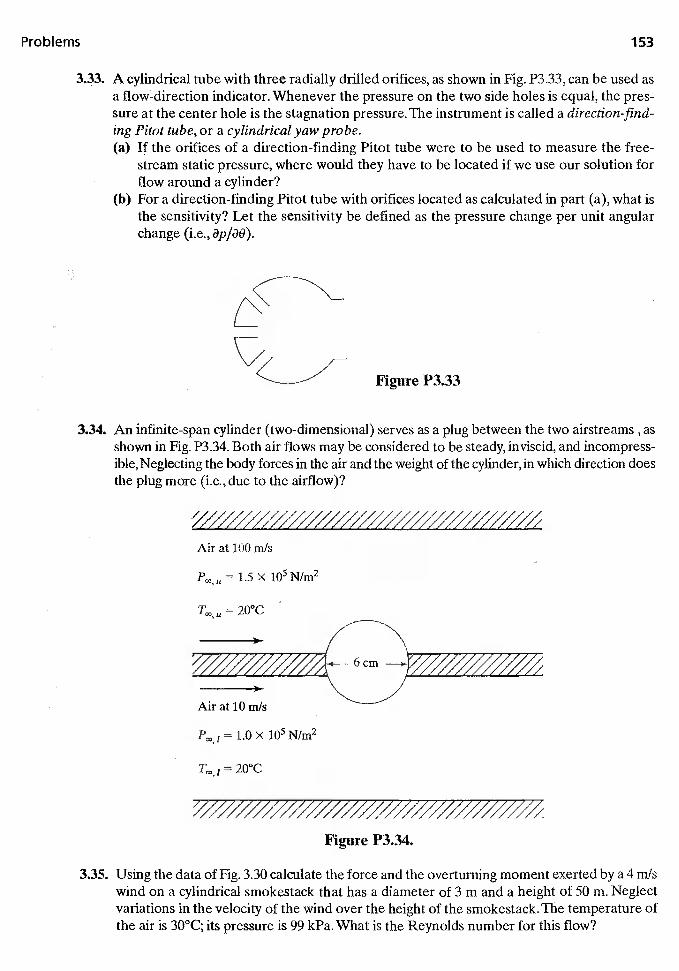
Problems 153
3.33. A cylindrical tube with three radially drilled orifices, as shown in Fig. P3.33, can be used asa flow-direction indicator. Whenever the pressure on the two side holes is equal, the pres-sure at the center hole is the stagnation pressure. The instrument is called a direction-find-ing Pitot tube, or a cylindrical yaw probe.(a) If the orifices of a direction-finding Pitot tube were to be used to measure the free-
stream static pressure, where would they have to be located if we use our solution forflow around a cylinder?
(b) For a direction-finding Pitot tube with orifices located as calculated in part (a), what isthe sensitivity? Let the sensitivity be defined as the pressure change per unit angularchange (i.e.,
Figure P3.33
3.34. An infinite-span cylinder (two-dimensional) serves as a plug between the two airstreams , as
shown in Fig. P3.34. Both air flows may be considered to be steady, inviscid, and incompress-ible, Neglecting the body forces in the air and the weight of the cylinder, in which direction doesthe plug more (i.e., due to the airflow)?
Air at 100 rn/s
= 1.5 X N/rn2
Air at 10 rn/s
F0,, = 1.0 X N/rn2
T0,,,=20°C
Figure P3.34.
335. Using the data of Fig. 3.30 calculate the force and the overturning moment exerted by a 4 rn/swind on a cylindrical smokestack that has a diameter of 3 m and a height of 50 m. Neglectvariations in the velocity of the wind over the height of the smokestack. The temperature ofthe air is 30°C; its pressure is 99 kPa. What is the Reynolds number for this flow?
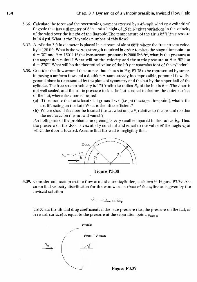
154 Chap. 3 I Dynamics of an Incompressible, Inviscid Flow Field
3.36. Calculate the force and the overturning moment exerted by a 45-mph wind on a cylindricalflagpole that has a diameter of 6 in. and a height of 15 ft. Neglect variations in the velocityof the wind over the height of the flagpole. The temperature of the air is 85°F; its pressureis 14.4 psi. What is the Reynolds number of this flow?
3.37. A cylinder 3 ft in diameter is placed in a stream of air at 68°F where the veloc-ity is 120 ft/s. What is the vortex strength required in order to place the stagnation points atO = 300 and 0 = 1500? If the free-stream pressure is 2000 lbf/ft2, what is the pressure atthe stagnation points? What will be the velocity and the static pressure at 0 = 90°? ato = 270°? What will be the theoretical value of the lift per spanwise foot of the cylinder?
3.38. Consider the flow around the quonset hut shown in Fig. P3.38 to be represented by super-imposing a unifonn flow and a doublet. Assume steady, incompressible, potential flow. Theground plane is represented by the plane of symmetry and the hut by the upper half of thecylinder. The free-stream velocity is 175 km/h; the radius R0 of the hut is 6 m. The door isnot well sealed, and the static pressure inside the hut is equal to that on the outer surfaceof the hut, where the door is located.(a) If the door to the hut is located at ground level (i.e., at the stagnation point), what is the
net lift acting on the hut? What is the lift coefficient?(b) Where should the door be located (i.e., at what angle relative to the ground) so that
the net force on the hut will vanish?For both parts of the problem, the opening is very small compared to the radius Thus,the pressure on the door is essentially constant and equal to the value of the angle 0o atwhich the door is located. Assume that the wall is negligibly thin.
= 175
3.39. Consider an incompressible flow around a semicylinder, as shown in Figure. P3.39. As-sume that velocity distribution for the windward surface of the cylinder is given by theinviscid solution
V = sin
Calculate the lift and drag coefficients if the base pressure (i.e., the pressure on the flat, orleeward, surface) is equal to the pressure at the separation point,
Pcomer
Pbase = Pcomer
Figure P3.39
Door
Figure P3.38
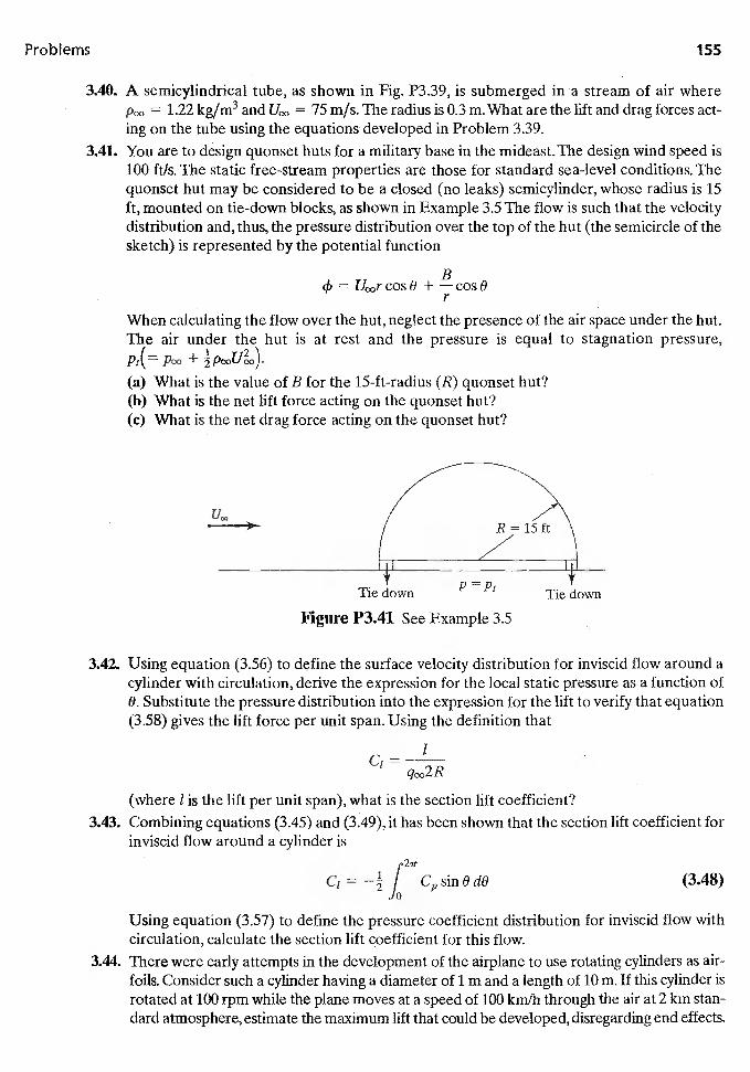
2ir
ci=
Problems
3.40. A semicylindrical tube, as shown in Fig. P3.39, is submerged in a stream of air where= 1.22 kg/rn3 and = 75 rn/s. The radius is 0.3 m.What are the lift and drag forces act-
ing on the tube using the equations developed in Problem 3.39.3.41. You are to design quonset huts for a military base in the mideast. The design wind speed is
100 ft/s. The static free-stream properties are those for standard sea-level conditions. Thequonset hut may be considered to be a closed (no leaks) semicylinder, whose radius is 15ft, mounted on tie-down blocks, as shown in Example 3.5 The flow is such that the velocitydistribution and, thus, the pressure distribution over the top of the hut (the semicircle of thesketch) is represented by the potential function
+
When calculating the flow over the hut, neglect the presence of the air space under the hut.The air under the hut is at rest and the pressure is equal to stagnation pressure,Pt(=(a) What is the value of B for the 15-ft-radius (R) quonset hut?(b) What is the net lift force acting on the quonset hut?(c) What is the net drag force acting on the quonset hut?
U..
Tie down Tie downp =p1
Figure P3.41 See Example 3.5
3.42. Using equation (3.56) to define the surface velocity distribution for inviscid flow around acylinder with circulation, derive the expression for the local static pressure as a function of0. Substitute the pressure distribution into the expression for the lift to verify that equation(3.58) gives the lift force per unit span. Using the definition that
C1=
(where 1 is the lift per unit span), what is the section lift coefficient?3.43. Combining equations (3.45) and (3.49), it has been shown that the section lift coefficient for
inviscid flow around a cylinder is
(3.48)
Using equation (3.57) to define the pressure coefficient distribution for inviscid flow withcirculation, calculate the section lift coefficient for this flow.
3.44. There were early attempts in the development of the airplane to use rotating cylinders as air-foils. Consider such a cylinder having a diameter of 1 m and a length of 10 m. If this cylinder isrotated at 100 rpm while the plane moves at a speed of 100 kmlh through the air at 2 km stan-dard atmosphere, estimate the maximum lift that could be developed, disregarding end effects.
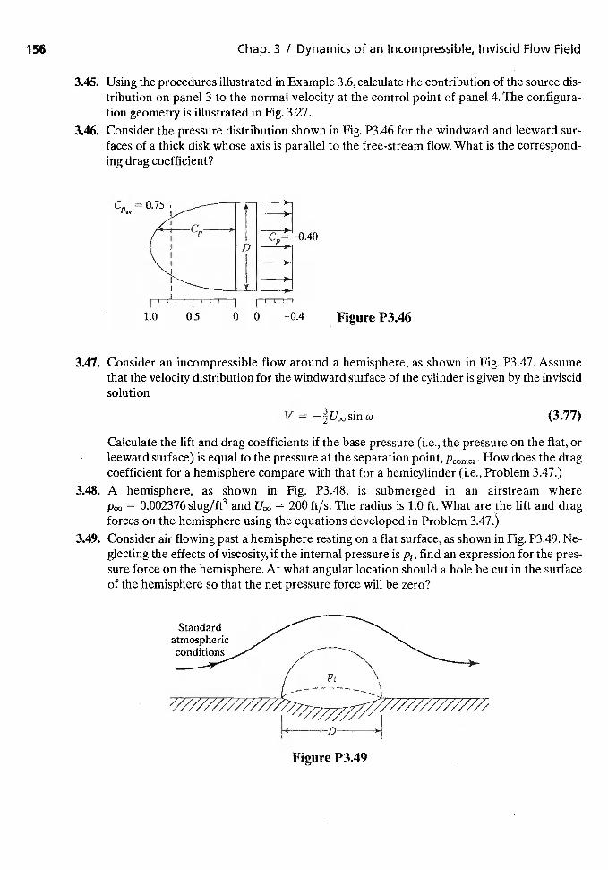
156 Chap. 3 / Dynamics of an Incompressible, Inviscid Flow Field
3.45. Using the procedures illustrated in Example 3.6, calculate the contribution of the. source dis-tribution on panel 3 to the normal velocity at the control point of panel 4. The configura-tion geometry is illustrated in Fig. 3.27.
3.46. Consider the pressure distribution shown in Fig. P3.46 for the windward and leeward sur-faces of a thick disk whose axis is parallel to the free-stream flow. What is the correspond-ing drag coefficient?
= 0.75 :I I
Figure P3.46
3.47. Consider an incompressible flow around a hemisphere, as shown in Fig. P3.47. Assumethat the velocity distribution for the windward surface of the cylinder is given by the inviscidsolution
V = (3.77)
Calculate the lift and drag coefficients if the base pressure (i.e., the pressure on the flat, orleeward surface) is equal to the pressure at the separation point, How does the dragcoefficient for a hemisphere compare with that for a hemicylinder (i.e., Problem 3.47.)
3.48. A hemisphere, as shown in Fig. P3.48, is submerged in an airstream where= 0.002376 slug/ft3 and = 200 ft/s. The radius is 1.0 ft. What are the lift and drag
forces on the hemisphere using the equations developed in Problem 3.47.)3.49. Consider air flowing past a hemisphere resting on a flat surface, as shown in Fig. P3.49. Ne-
glecting the effects of viscosity, if the internal pressure is find an expression for the pres-sure force on the hemisphere. At what angular location should a hole be cut in the surfaceof the hemisphere so that the net pressure force will be zero?
Figure P3.49
Standardatmospheric
D
References 157
3.50. A major league pitcher is accused of hiding sandpaper in his back pocket in order to scuffup an otherwise "smooth" basebalL Why would he do this? To estimate the Reynolds num-ber of the baseball, assume its speed to be 90 mi/h and its diameter 2.75 in.
3.51. Derive the stream functions for the elementary flows of Table 3.2.3.52. What condition(s) must prevail in order for a velocity potential to exist? For a stream func-
tion to exist?
REFERENCES
Achenbach E. 1968. Distributions of local pressure and skin friction around a circular cylin-der in cross flow up to Re = 5 X 10⁶. J, Fluid Mechanics 34:625—639
Campbell J, Chambers JR. 1994. Patterns in the sky: natural visualization of aircraft flowfields. NASA SP-514
Hess JL, Smith AMO. 1967. Calculations of potential flow about arbitrary bodies. Progr.Aeronaut. Sci. 8:1-138
Hoerner SF. 1958. Fluid Dynamic Drag. Midland Park, NJ: published by the author
Hoerner SF, Borst liv. 1975. Fluid Dynamic Lift. Midland Park, NJ: published by theauthorsKellogg OD. 1953. Fundamentals of Potential Theory. New York: Dover
Schlichting H. 1968. Boundary Layer Theory. 6th Ed. New York: McGraw-Hill
Talay TA. 1975. Introduction to the aerodynamics of flight. NASA SP-367
1976. U.S. Standard Atm osphere. Washington, DC: U.S. Government Printing Office
4 VISCOUS BOUNDARY
LAYERS
The equation for the conservation of linear momentum was developed in Chapter 2 byapplying Newton's law, which states that the net force acting on a fluid particle is equalto the time rate of change of the linear momentum of the fluid particle. The principalforces considered were those that act directly on the mass of the fluid element (i.e., thebody forces) and those that act on its surface (i.e., the pressure forces and shear forces).The resultant equations are known as the Navier-Stokes equations. Even today, there areno general solutions for the complete Navier-Stokes equations. Nevertheless, reason-able approximations can be introduced to describe the motion of a viscous fluid if theviscosity is either very large or very small. The latter case is of special interest to us, sincetwo important fluids, water and air, have very small viscosities. Not only is the viscosityof these fluids very small, but the velocity for many of the practical applications relevantto this text is such that the Reynolds number is very large.
Even in the limiting case where the Reynolds number is large, it is not permissiblesimply to omit the viscous terms completely, because the solution of the simplified equa-tion could not be made to satisfy the complete boundary conditions. However, for manyhigh Reynolds number flows, the flow field may be divided into two regions: (1) a viscousboundary layer adjacent to the surface of the vehicle and (2) the essentially inviscid flowOutside the boundary layer, The velocity of the fluid particles increases from a value ofzero (in a vehicle-fixed coordinate system) at the wall to the value that corresponds tothe external "frictionless" flow outside the boundary layer. Outside the boundary layer,
Sec. 4.1 I Equations Governing the Boundary Layer for a Incompressible How 159
the transverse velocity gradients become so small that the shear stresses acting on a fluidelement are negligibly small. Thus, the effect of the viscous terms may be ignored whensolving for the flow field external to the boundary layer.
When using the two-region flow model to solve for the flow field, the first step isto solve for the iñviscid portion of the flow field. The solution for the inviscid portion ofthe flow field must satisfy the boundary conditions: (1) that the velocity of the fluid par-ticles far from the body be equal to the free-stream value and (2) that the velocity of thefluid particles adjacent to the body parallel to the "surface." The second boundarycondition represents the physical requirement that there is no flow through a solid sur-face. However, since the flow is iñviscid, the velocity component parallel to the surfacedoes not have to be zero. Having solved for the inviscid flow field, the second step is tocalculate the boundary layer using the inviscid flow as the outer boundary condition.
If the boundary layer is relatively thick, it may be necessary to use an iterative processfor calculating the flow field. To start the second iteration, the inviscid flow field is recal-culated, replacing the actual configuration by the "effective" configuratiOn, which is deter-mined by adding the displacerne it thickness of the boundary layer from the first iterationto the surface coordinate of the actual configuration. See Fig. 2.13. The boundary layer isrecalculated using the second-iterate inviscid flow as the boundary condition.As discussedin DeJarnette and Ratcliffe (1996), the iterative procedure required to converge to a solu-tion requires an understanding of each region of the flow field and their interactions.
In Chapter 3; we generated solutions for the inviscid flow field for a variety of con-figurations. In this chapter we examine the viscous region in detail, assuming that the in-viscid flow field is known.
4.1 EQUATIONS GOVERNING THE BOUNDARY LAYERFOR A STEADY, TWO-DIMENSIONAL,INCOMPRESSIBLE FLOW
In this chapter, we discuss techniques by which we can obtain engineering solutionswhen the boundary layer is either laminar or tUrbulent. Thus, for the purpose of thistext, we shall assume that we know whether the boundary layer is laminar or turbulent.The transition process through which the boundary layer "transitions" from a laminarstate to a turbulent state is quite complex and depends on many parameters (e.g., sur-face roughness, surface temperature, pressure gradient, and Mach number). A brief sum-mary of the factors affecting transition is presented later in this chapter. For a moredetailed discussion of the parameters that affect transition, the reader is referred toSchlichting (1979) and White (2005).
To simplify the development of the solution techniques, we will consider the flowto be steady, two-dimensional, and constant property (or, equivalently, incompressiblefor a gas flow). By restricting ourselves to such flows, we can concentrate on the devel-opment of the solution techniques themselves. As shown in Fig. 4.1, the coordinate sys-tem is fixed to the surface of the, body. The x coordinate is measured in the streamwisedirection along the surface of the configuration. The stagnation point (or the leadingedge if the configuration is a sharp object) is at x = 0. The y coordinate is perpendicu-lar to the surface. This coordinate system is used throughout this chapter.
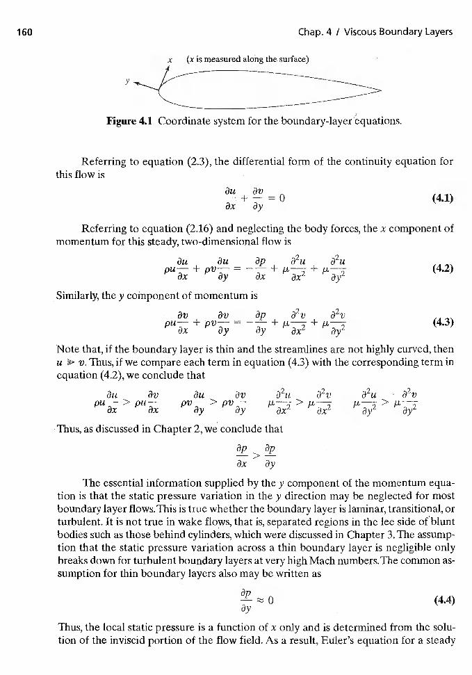
160 Chap. 4 I Viscous Boundary Layers
x is measured along the surface)
Figure 4.1 Coordinate system for the boundary-layer equations.
Referring to equation (2.3), the differential form of the continuity equation forthis flow is
(4.1)ax 8y
Referring to equation (2.16) and neglecting the body forces, the x component ofmomentum for this steady, two-dimensional flow is
au a2u(4.2)
äx ay
Similarly, the y component of momentum is
t3V 3p(4.3)
ax ay
Note that, if the boundary layer is thin and the streamlines are not highly curved, thenu v. Thus, if we compare each term in equation (4.3) with the corresponding term inequation (4.2), we conclude that
au au a2v 82vPu— > pu— pV > pV—
ax äy 3y 8x c3y
Thus, as discussed in Chapter 2, we conclude that
ax ay
The essential information supplied by the y component of the momentum equa-tion is that the static pressure variation in the y direction may be neglected for mostboundary layer flows. This is true whether the boundary layer is laminar, transitional, orturbulent. It is not true in wake flows, that is, separated regions in the lee side of bluntbodies such as those behind cylinders, which were discussed in Chapter 3.The assump-tion that the static pressure variation across a thin boundary layer is negligible onlybreaks down for turbulent boundary layers at very high Mach numbers. The common as-sumption for thin boundary layers also may be written as
(4.4)
Thus, the local static pressure is a function of x only and is determined from the solu-tion of the inviscid portion of the flow field. As a result, Euler's equation for a steady
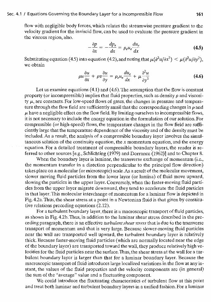
Sec. 4.1 / Equations Governing the Boundary Layer for a Incompressible Flow 161
flow with negligible body forces, which relates the streamwise pressure gradient to thevelocity gradient for the inviscid flow, can be used to evaluate the pressure gradient inthe viscous region, also.
dUe—— = = PeUeT (45)ax ax
Substituting equation (4.5) into equation (4.2), and noting that <we obtain
t3u äu dUe 32uPu— + pV = + (4.6)
dx
Let us examine equations (4.1) and (4.6).The assumption that the flow is constantproperty (or incompressible) implies that fluid properties, such as density p and viscosi-ty are constants. For low-speed flows of gases, the changes in pressure and tempera-ture through the flow field are sufficiently small that the corresponding changes in p and1a have a negligible effect on the flow field. By limiting ourselves to incompressible flows,it is not necessary to include the energy equation in the formulation of our solution. Forcompressible (or high-speed) flows, the temperature changes in the flow field are suffi-ciently large that the temperature dependence of the viscosity and of the density must beincluded. As a result, the analysis of a compressible boundary layer involves the simul-taneous solution of the continuity equation, the x momentum equation, and the energyequation. For a detailed treatment of compressible boundary layers, the reader is re-ferred to other sources [e.g., Schlichting (1979) and Dorrance (1962)3 and to Chapter 8.
When the boundary layer is laminar, the transverse exchange of momentum (i.e.,the momentum transfer in a direction perpendicular to the principal flow direction)takes place on a molecular (or microscopic) scale. As a result of the molecular movement,slower moving fluid particles from the lower layer (or lamina) of fluid move upward,slowing the particles in the upper layer. Conversely, when the faster-moving fluid parti-cles from the upper layer migrate downward, they tend to accelerate the fluid particlesin that layer. This molecular interchange of momentum for a laminar flow is depicted inFig. 4.2a. Thus, the shear stress at a point in a Newtonian fluid is that given by constitu-tive relations preceding equations (2.12).
For a turbulent boundary layer, there is a macroscopic transport of fluid particles,as shown in Fig. 4.2b. Thus, in addition to the laminar shear stress described in the pre-ceding paragraph, there is an effective turbulent shear stress that is due to the transversetransport of momentum and that is very large. Because slower-moving fluid particlesnear the wall are transported well upward, the turbulent boundary layer is relativelythick. Because faster-moving fluid particles (which are normally located near the edgeof the boundary layer) are transported toward the wall, they produce relatively high ye-locities for the fluid particles near the surface.Thus, the shear stress at the wall for a tur-bulent boundary layer is larger than that for a laminar boundary layer. Because themacroscopic transport of fluid introduces large localized variations in the flow at any in-stant, the values of the fluid properties and the velocity components are (in general)the sum of the "average" value and a fluctuating component.
We could introduce the fluctuating characteristics of turbulent flow at this pointand treat both laminar and turbulent boundary layers in a unified fashion. For a laminar
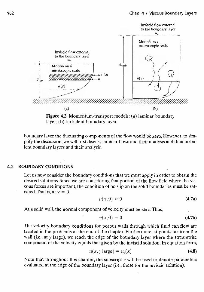
162 Chap. 4 I Viscous Boundary Layers
Inviscid flow externalto the boundary layer
__________
Ue
Motion on amacroscopic scale
Inviscid flow externalto the boundary layer
iLe
F MotiononalmicrOscopic scale
-u u(y)
(a) (b)
Figure 4.2 Momentum-transport models: (a) laminar boundarylayer; (b) turbulent boUndary layer.
boundary layer the fluctuating components of the flow would be zero. However, to sim-plify the discussion, we will first discuss laminar flOws and their analysis and then turbu-lent boundary layers and their analysis.
4.2 BOUNDARY CONDITIONS
Let us now consider the boundary conditions that we must apply in order to obtain thedesired solutions. Since we are considering that portion of the flow field where the vis-cous forces are important, the condition of no slip on the solid boundaries must be sat-isfied.Thatis,aty = 0,
u(x,0) = 0 (4.7a)
At a solid wall, the normal component of velocity must be zero. Thus,
v(x,O) 0 (4.7b)
The velocity boundary conditions for porous walls through which fluid can flow aretreated in the problems at the end of the chapter. Furthermore, at points far from thewall (i.e., at y large), we reach the edge of the boundary layer where the streamwisecomponent of the velocity equals that given by the inviscid solution. In equation form,
u(x,ylarge) Ue(X) (4.8)
Note that throughout this chapter, the subscript e will be used to denote parametersevaluated at the edge of the boundary layer (i.e., those for the inviscid solution).
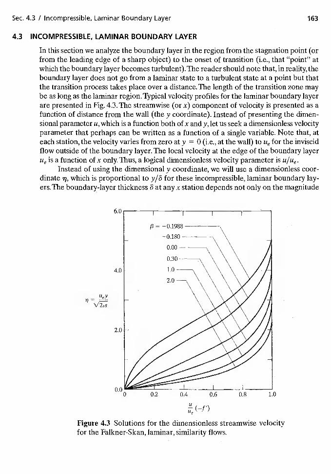
Sec. 4.3 I Incompressible, Laminar Boundary Layer 163
43 INCOMPRESSIBLE, LAMINAR BOUNDARY LAYER
In this section we analyze the boundary layer in the region from the stagnation point (orfrom the leading edge of a sharp object) to the onset of transition (i.e., that "point" atwhich the boundary layer becomes turbulent).The reader should note that, in reality, theboundary layer does not go from a laminar state to a turbulent state at a point but thatthe transition process takes place over a distance. The length of the transition zone maybe as long as the laminar region. Typical velocity profiles for the laminar boundary layerare presented in Fig. 4.3. The streamwise (or x) component of velocity is presented as afunction of distance from the wall (the y coordinate). Instead of presenting the dimen-sional parameter u, which is a function both of x and y, let us seek a dimensionless velocityparameter that perhaps can be written as a function of a single variable. Note that, ateach station, the velocity varies from zero at y = 0 (i.e., at the wall) to Ue for the inviscidflow outside of the boundary layer. The local velocity at the edge of the boundary layerUe is a function of x only. Thus, a logical dimensionless velocity parameter is U/Ue.
Instead of using the dimensional y coordinate, we will use a dimensionless coor-dinate which is proportional to y/6 for these incompressible, laminar boundary lay-ers.The boundary-layer thickness 6 at any x station depends not only on the magnitude
—11
Figure 4.3 Solutions for the dimensionless streamwise velocityfor the Falkner-Skan, laminar, similarity flows.
0 0.2 0.4 0.6 0.8 1.0
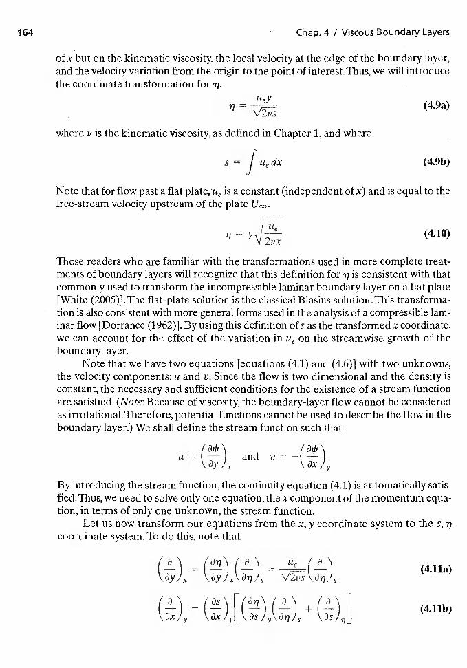
164 Chap. 4 / Viscous Boundary Layers
of x but on the kinematic viscosity, the local velocity at the edge of the boundary layer,and the velocity variation from the origin to the point of interest.Thus, we will introducethe coordinate transformation for
UeY77
=(49a)
where i' is the kinematic viscosity, as defined in Chapter 1, and where
s= f dx (4..9b)
Note that for flow past a flat plate;ue is a constant (independent of x) and is equal to thefree-stream velocity upstream of the plate
= (4.10)
Those readers who are familiar with the transformations used in more complete treat-ments of boundary layers will recognize that this definition for is consistent with thatcommonly used to transform the incompressible laminar boundary layer on a flat plate[White (2005)]. The flat-plate solution is the classical Blasius solution. Thistion is also consistent with more general forms used in the analysis of a compressible lam-inar flow {Dorrance (1962)]. By using this definition of s as the transformed x coordinate,we can account for the effect of the variation in Ue on the streamwise growth of theboundary layer.
Note that we have two equations [equations (4.1) and (4.6)] with two unknowns,the velocity components: u and v. Since the flow is two dimensional and the density isconstant, the necessary and sufficient conditions for the existence of a stream functionare satisfied. (Note: Because of viscosity, the boundary-layer flow cannot be consideredas irrotationaL Therefore, potential functions cannot be used to describe the flow in theboundary layer.) We shall define the stream function such that
u=t—I and v=—I------'\ax
By introducing the stream function, the continuity equation (4.1) is automatically satis-fied.Thus,we need to solve only one equation, thex component of the momentum equa-tion, in terms of only one unknown, the stream function.
Let us now transform our equations from the x, y coordinate system to the s,coordinate system. To do this, note that
= e (4.lla)\'ayJx \\aYJ'X'\aTlJS
+ 1 (4.llb)
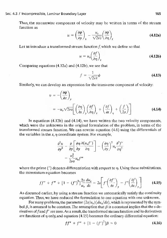
Sec. 4.3 1 Incompressible, Laminar Boundary Layer 165
Thus, the streamwise component of velocity may be written in terms of the streamfunction as
==
(4.12a)
Let us introduce a transformed stream function f, which we define so that
u = (4.12b)&y1 S
Comparing equations (4.12a) and (4J2b), we see that
1(4.13)
Similarly, we can develop an expression for the transverse component of velocity:
V = —t —
+ + (4.14)
In equations (4.12b) and (4.14), we have written the two velocity components,which were the unknowns in the original formulation of the problem, in terms of thetransformed stream function. We can rewrite equation (4.6) using the differentials ofthe variables in the s, 1) coordinate system. For example,
82u a [aiia(uef')l= = ( I
äy2 J2
=2vs
where the prime (') denotes differentiation with respect to vj. Using these substitutions,the momentum equation becomes
ff" + f" + [1 - (f1)21 - (4.15)
As discussed earlier, by using a stream function we automatically satisfy the continuityequation. Thus, we have reduced the formulation to one equation with one unknown.
For many problems, the parameter (2S/Ue) ( due/ds), which is represented by the sym-bol /3, is assumed to be constant. The assumption that /3 is a constant implies that the s de-rivatives of f and f' are zero.As a result, the transformed stream function and its derivativesare functions of only, and equation (4.15) becomes the ordinary differential equation:
+ fill + [1 — (f')2]/3 = 0 (4.16)
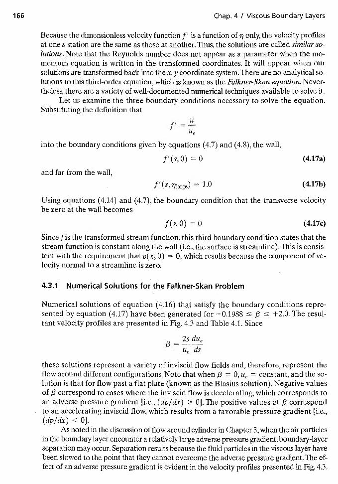
166 Chap. 4 / Viscous Boundary Layers
Because the dimensionless velocity function f' is a function of ij only, the velocity profilesat one s station are the same as those at another. Thus, the solutions are called similar so-lutions. Note that the Reynolds number does not appear as a parameter when the mo-mentum equation is written in the transformed coordinates. It will appear when oursolutions are transformed back into the x, y coordinate system. There are no analytical so-lutions to this third-order equation, which is known as the Falkner-Skan equation. Never-theless, there are a variety of well-documented numerical techniques available to solve it.
Let us examine the three boundary conditions necessary to solve the equation.Substituting the definition that
Ue
into the boundary conditions given by equations (4.7) and (4.8), the wall,
f'(s,O) = 0 (4.17a)
and far from the wall,
= 1.0 (4.17b)
Using equations (4.14) and (4.7), the boundary condition that the transverse velocitybe zero at the wall becomes
f(s,0) = 0 (4.17c)
Since f is the transformed stream function, this third boundary condition states that thestream function is constant along the wall (i.e., the surface is streamline).This is consis-tent with the requirement that v(x, 0) = 0, which results because the component of ve-locity normal to a streamline is zero.
4.3.1 Numerical Solutions for the Falkner-Skan Problem
Numerical solutions of equation (4.16) that satisfy the boundary conditions repre-sented by equation (4.17) have been generated for —0.1988 � � +2.0. The resul-tant velocity profiles are presented in Fig. 4.3 and Table 4.1. Since
= 2s dUe
ds
these solutions represent a variety of inviscid flow fields and, therefore, represent theflow around different configurations. Note that when f3 = 0, Ug = constant, and the so-lution is that for flow past a flat plate (known as the Blasius solution). Negative valuesof /3 correspond to cases where the inviscid flow is decelerating, which corresponds toan adverse pressure gradient [i.e., (dp/dx) > 0]. The positive values of /3 correspondto an accelerating inviscid flow, which results from a favorable pressure gradient [i.e.,(dp/dx) <0].
As noted in the discussion of flow around cylinder in Chapter 3, when the air particlesin the boundary layer encounter a relatively large adverse pressure gradient, boundary-layerseparation may occur. Separation results because the fluid particles in the viscous layer havebeen slowed to the point that they cannot overcome the adverse pressure gradient. The ef-fect of an adverse pressure gradient is evident in the velocity profiles presented in Fig. 4.3.
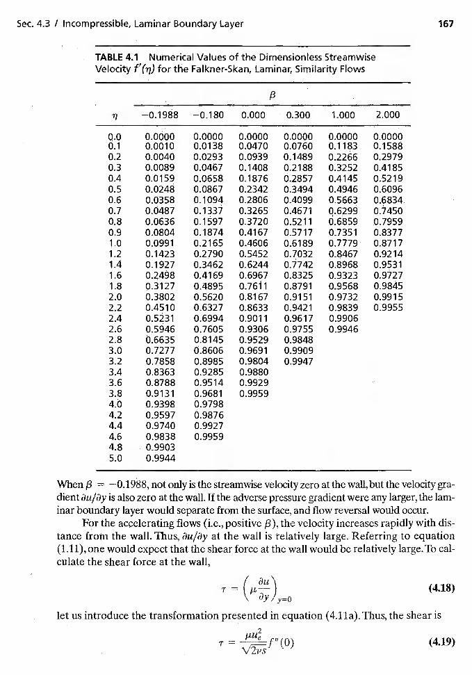
Sec. 4.3 I incompressible, Laminar Boundary Layer 167
TABLE 4.1 Nurnerica I Values of the Dimensionless StreamwiseVelocity f'(n) for the Falkner-Skan, Laminar, Similarity Flows
/3
—0.1988 —0.180 0.000 0.300 1.000 2.000
0.0 0.0000 0.0000 0.0000 0.0000 0.0000 0.00000.1 0.0010 0.0138 0.0470 0.0760 0.1183 0.15880.2 0.0040 0.0293 0.0939 0.1489 0.2266 0.29790.3 0.0089 0.0467 0.1408 0.2188 0.3252 0.41850.4 0.0159 0.0658 0.1876 0.2857 0.4145 0.52190.5 0.0248 0.0867 0.2342 0.3494 0.4946 0.60960.6 0.0358 0.1094 0.2806 0.4099 0.5663 0.6834.0.7 0.0487 0.1337 0.3265 0.4671 0.6299 0.74500.8 0.0636 0.1597 0.3720 0.5211 0.6859 0.79590.9 0.0804 0.1874 0.4167 0.5717 0.7351 0.83771.0 0.0991 0.2165 0.4606 0.6189 0.7779 0.87171.2 0.1423 0.2790 0.5452 0.7032 0.8467 0.92141.4 0.1927 0.3462 0.6244 0.7742 0.8968 0.95311.6 0.2498 0.4169 0.6967 0.8325 0.9323 0.97271.8 0.3127 0.4895 0.7611 0.8791 0.9568 0.98452.0 0.3802 0.5620 0.8167 0.9151 0.9732 0.99152.2 0.4510 0.6327 0.8633 0.9421 0.9839 0.99552.4 0.5231 0.6994 0.9011 0.9617 0.99062.6 0.5946 0.7605 0.9306 0.9755 0.99462.8 0.6635 0.8145 0.9529 0.98483.0 0.7277 0.8606 0.969 1 0.99093.2 0.7858 0.8985 0.9804 0.99473.4 0.8363 0.9285 0.98803.6 0.8788 0.9514 0.99293.8 0.9131 0.9681 0.99594.0 0.9398 0.97984.2 0.9597 0.98764.4 0.9740 0.99274.6 0.9838 0.99594.8 0.99035.0 0.9944
When /3 = —0.1988, not only is the streamwise velocity zero at the wall, but the velocity gra-dient au/ay is also zero at the wall. If the adverse pressure gradient were any larger, the lam-inar boundary layer would separate from the surface, and flow reversal would occur.
For the accelerating flows (i.e., positive /3), the velocity increases rapidly with dis-tance from the wall. Thus, au/ay at the wall is relatively large. Referring to equation(1.11), one would expect that the shear force at the wall would be relatively large.To cal-culate the shear force at the wall,
T=
(4.18)dy
let us introduce the transformation presented in equation (4.lla).Thus, the shear is
T=
(4.19)
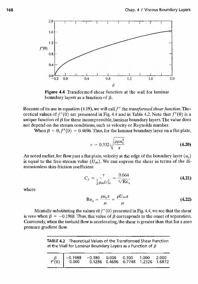
Figure 4.4 Transformed shear function at the wall for laminarboundary layers as a function of f3.
2.0
TABLE 4.2 Theoretical Values of the Transformed Shear Functionat the Walt for Laminar Boundary Layers as a Function of
$ —0.1988 —0.180 0.000 0.300 1.000 2.000f"(O) 0.000 0.1286 0.4696 0.7748 1.2326 1.6872
168 Chap. 4 I Viscous Boundary Layers
f "(0)
13
Because of its use in equation (4.19), we will call f" the transformed shear function.The-oretical values of f" (0) are presented in Fig. 4.4 and in Table 4.2. Note that f" (0) is aunique function of /3 for these incompressible, laminar boundary layers. The value doesnot depend on the stream conditions, such as velocity or Reynolds number.
When /3 = 0, f" (0) = 0.4696. Thus, for the laminar boundary layer on a flat plate,
T = (4.20)
As noted earlier, for flow past a flat plate, velocity at the edge of the boundary layer (tie)is equal to the free-stream value We can express the shear in terms of the di-mensionless skin-friction coefficient
T 0.664
=(4.21)
where
=(4.22)
Mentally substituting the values off" (0) presented in Fig. 4.4, we see that the shearis zero when /3 = —0.1988. Thus, this value of /3 corresponds to the onset of separation.Conversely, when the inviscid flow is accelerating, the shear is greater than that for a zeropressure gradient flow.
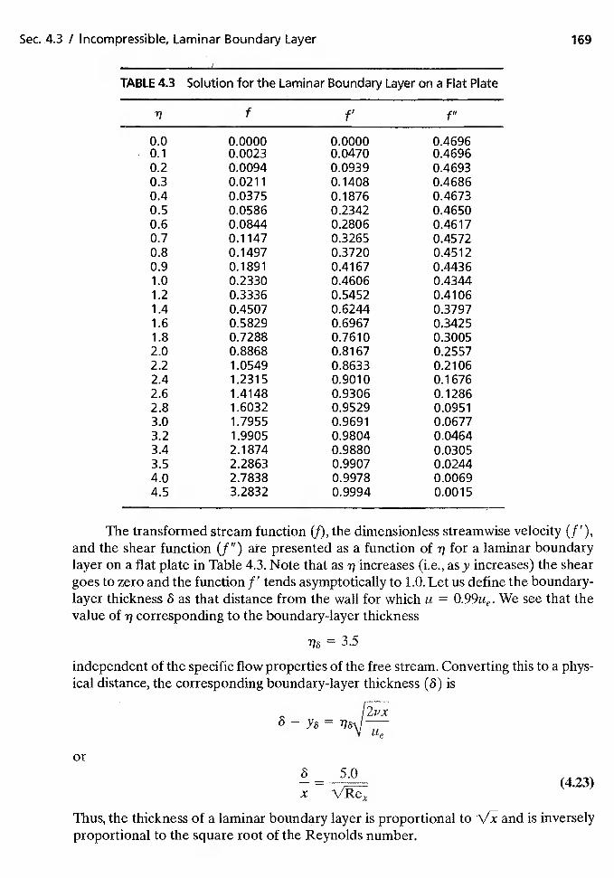
Sec. 4.3 / Incompressible, Laminar Boundary Layer 169
TAB LE 4.3 Solution for the Lammar Boundary Layer on a Flat Plate
lj f f' f"
0.0 0.0000 0.0000 0.4696• 0.1 0.0023 0.0470 0.4696
0.2 0.0094 0.0939 0.46930.3 0.0211 0.1408 0.46860.4 0.0375 0.1876 0.46730.5 0.0586 0.2342 0.46500.6 0.0844 0.2806 0.46170.7 0.1 147 0.3265 0.45720.8 0.1497 0.3720 0.45120.9 0.1891 0.4167 0.44361.0 0.2330 0.4606 0.43441.2 0.3336 0.5452 0.41061.4 0.4507 0.6244 0.37971.6 0.5829 0.6967 0.34251.8 0.7288 0.7610 0.30052.0 0.8868 0.8167 0.25572.2 1.0549 0.8633 0.21062.4 1.2315 0.9010 0.16762.6 1.4148 0.9306 0.12862.8 1.6032 0.9529 0.09513.0 1.7955 0.9691 0.06773.2 1.9905 0.9804 0.04643.4 2.1874 0.9880 0.03053.5 2.2863 0.9907 0.02444.0 2.7838 0.9978 0.00694.5 3.2832 0.9994 0.0015
The transformed stream function (f), the dimensionless streamwise velocity (f'),and the shear function (f") are presented as a function of for a laminar boundarylayer on a flat plate in Table 4.3. Note that as increases (i.e., as y increases) the sheargoes to zero and the function f' tends asymptotically to 1.0. Let us define the boundary-layer thickness 6 as that distance from the wall for which u = O.99Ue. We see that thevalue of q corresponding to the boundary-layer thickness
independent of the specific flow properties of the free stream. Converting this to a phys-ical distance, the corresponding boundary-layer thickness (6) is
6 = =
or6 5.0— — (4.23)
Thus, the thickness of a laminar boundary layer is proportional to and is inverselyproportional to the square root of the Reynolds number.
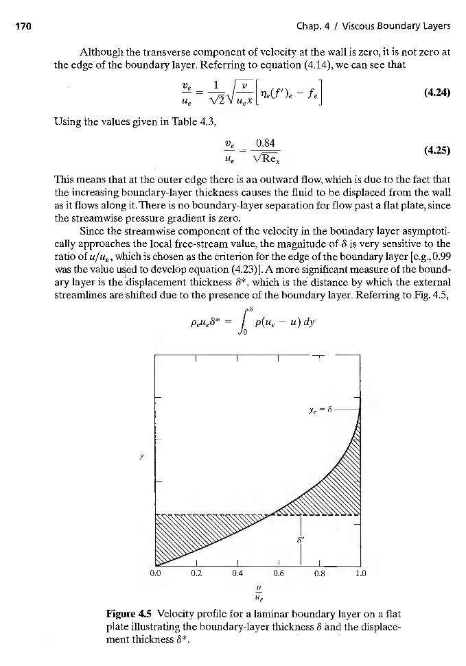
Ve 1 - fe]
U
1te
Figure 4.5 Velocity profile for a laminar boundary layer on a flatplate illustrating the boundary-layer thickness 6 and the displace-ment thickness
170 Chap. 4 / Viscous Boundary Layers
Although the transverse component of velocity at the wall is zero, it is not zero atthe edge of the boundary layer. Referring to equation (4.14), we can see that
(4.24)
Using the values given in Table 4.3,
Ve 0.84425
This means that at the outer edge there is an outward flow, which is due to the fact thatthe increasing boundary-layer thickness causes the fluid to be displaced from the wallas it flows along it. There is no boundary-layer separation for flow past a flat plate, sincethe streamwise pressure gradient is zero.
Since the streamwise component of the velocity in the boundary layer asymptoti-cally approaches the local free-stream value, the magnitude of 8 is very sensitive to theratio of U/tie, which is chosen as the criterion for the edge of the boundary layer [e.g., 0.99was the value used to develop equation (4.23)].A more significant measure of the bound-ary layer is the displacement thickness 8*, which is the distance by which the externalstreamlines are shifted due to the presence of the boundary layer. Referring to Fig. 4.5,
y
p8
Petie6*= J
p(Ue — u) dy0
0.0
Sec. 4.3 / Incompressible, Laminar Boundary Layer 171
Thus, for any incompressible boundary layer,
6*=
—
dy (4.26)
Note that, since the integrand is zero for any point beyond 8, the upper limit for the in-tegration does not matter providing it is equal to (or greater than) 6. Substituting thetransformation of equation (4.10) for the laminar boundary layer on a flat plate,
6* = —
Using the values presented in Table 4.3, we obtain
6* = — fe) 1.72(4.27)
Thus, for a flat plate at zero incidence in a uniform stream, the displacement thickness6* is on the order of one-third the boundary-layer thickness 6.
The momentum thickness, 0, for an incompressible boundary layer is given by
o = dy (4.28)O Ue\
The momentum thickness represents the height of the free-stream flow which would beneeded to make up the deficiency in momentum flux within the boundary layer due tothe shear force at the surface. For an incompressible, laminar boundary layer,
o — 0.664429
Another convenient formulation for skin-friction on a flat plate is found by inte-grating the "local" skin-friction coefficient, Cf, found in equation (4.21) to obtain a"total" or "average" skin-friction drag coefficient on the flat plate [White (2005)]. Theuse of the total skin-friction drag coefficient avoids performing the same integrationnumerous times with different flat-plate lengths accounting for different results, Thetotal skin-friction coefficient is defined as
Cf (4.30)
where D1 is the friction drag on the plate and 5wet is the wetted area of the plate (thewetted area is the area of the plate in contact with the fluid—for one side of the plate,Swet = Lb).The total skin-friction coefficient for laminar boundary layers becomes
1 b1.L
Cf= bJ rdx=o o
1 0.664 28= 2Cf(L) = 7 (4.31)
172 Chap. 4 / Viscous Boundary Layers
which is just twice the value of the local skin-friction coefficient evaluated at x = L.The total skin-friction coefficient for laminar flow simply becomes
— 1.328C1
=(4.32)
where ReL is the Reynolds number evaluated at x = L, which is the end of the flatplate.
Since drag coefficients are normally nondimensionalized by a reference area ratherthan a wetted area [see equation (3.53)], the drag coefficient due to skin-friction is ob-tained from equation (4.30) as
Df SCD = = (4.33)
-'ref
It can be tempting to add together the total skin-friction coefficients for variousflat plates in order to obtain a total skin-friction drag—this must never be done! Sinceeach total skin-friction coefficient is defined with a different wetted area, doing thiswould result in an incorrect result. In other words,
N
Cfi= 1
Always convert total skin-friction coefficients into drag coefficients (based on a singlereference area) and then add the drag coefficients to obtain a total skin-friction dragcoefficient:
N
CD = CD. (4.34)i=1
EXAMPLE 4.1:
A rectangular plate, whose streamwise dimension (or chord c) is 0.2 rn andwhose width (or span b) is 1.8 rn,is mounted in a wind tunnel.The free-streamvelocity is 40 rn/s. The density of the air is 1.2250 kg/rn3, and the absolute vis-cosity is 1.7894 >< kg/rn. s. Graph the velocity profiles at x = 0.0 m,x = 0.05 m, x = 0.10 m, and x = 0.20 m. Calculate the chordwise distribu-tion of the skin-friction coefficient and the displacement thickness. What is thedrag coefficient for the plate?
Solution: Since the span (or width) of the plate is 9.0 times the chord (or streamwisedimension), let us assume that the flow is two dimensional (i.e., it is inde-pendent of the spanwise coordinate). The maximum value of the localReynolds number, which occurs when x = c, is
(1.225 kg/m3)(40m/s)(0.2 m)= 5.477 X
(1.7894 X105kg/m.s)
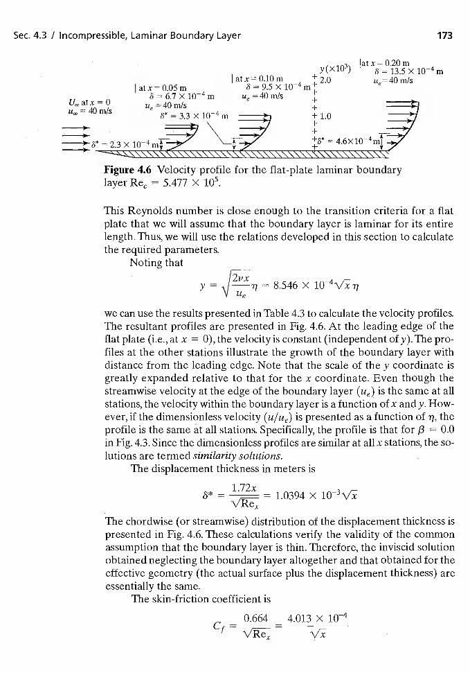
Sec. 4.3 / Incompressible, Laminar Boundary Layer 173
Iatx=O.20my(X1O) 13.5 X 10⁴mIatx=O.lOm u =40m/s
Iatx=O.05m8=6.7X1O4m ue=40m/s +
U00=40fl1/S
+
2.3 x
Figure 4.6 Velocity profile for the laminar boundarylayer = 5.477 X i05.
This Reynolds number is close enough to the transition criteria for a flatplate that we will assume that the boundary layer is laminar for its entirelength. Thus, we will use the relations developed in this section to calculatethe required parameters.
Noting that
y = = 8.546 xtIe
we can use the results presented in Table 4.3 to calculate the velocity profiles.The resultant profiles are presented in Fig. 4.6. At the leading edge of theflat plate (i.e., at x = 0), the velocity is constant (independent of y).The pro-files at the other stations illustrate the growth of the boundary layer withdistance from the leading edge. Note that the scale of the y coordinate isgreatly expanded relative to that for the x coordinate. Even though thestreamwise velocity at the edge of the boundary layer (ue) is the same at allstations, the velocity within the boundary layer is a function of x and y. How-ever, if the dimensionless velocity (U/tie) is presented as a function of theprofile is the same at all stations. Specifically, the profile is that for /3 = 0.0in Fig. 4.3. Since the dimensionless profiles are similar at all x stations, the so-lutions are termed similarity solutions.
The displacement thickness in meters is
= 1.72x= L0394 x
The chordwise (or streamwise) distribution of the displacement thickness ispresented in Fig. 4.6. These calculations verify the validity of the commonassumption that the boundary layer is thin. Therefore, the inviscid solutionobtained neglecting the boundary layer altogether and that obtained for theeffective geometry (the actual surface plus the displacement thickness) areessentially the same.
The skin-friction coefficient is
0.664 4.013 x
+++ 1.0+
174 Chap. 4 / Viscous Boundary Layers
Let us now calculate the drag coefficient for the plate. Obviously, thepressure contributes nothing to the drag. Therefore, the drag force acting onthe flat plate is due only to skin friction. Using general notation, we see that
PC
D = 2b / TdX (4.35)
We need integrate only in the x direction, since by assuming the flow to betwo dimensional, we have assumed that there is no spanwise variation in theflow. In equation (4.35), the integral, which represents the drag per unit width(or span) of the plate, is multiplied by b (the span) and by 2 (since frictionacts on both the top and bottom surfaces of the plate). Substituting the ex-pression for the laminar shear forces, given in equation (4.20),
D
= (4.36)
Since the edge velocity (ue) is equal to the free-stream velocity thedrag coefficient for the plate is, therefore,
D 2.656CD
=(437)
For the present problem, CD = 3.589 X
Alternatively, using the total skin-friction coefficient equation (4.32)and computing drag on the top and bottom of the plate,
1.328 2Lb —CD—Cf —3.589x10Sref Lb
EXAMPLE 4.2:
The streamwise velocity component for a laminar boundary layer is some-times assumed to be roughly approximated by the linear relation
yU =
where = 1.25 x 10_2 Assume that we are trying to approximate theflow of air at standard sea-level conditions past a flat plate whereUe = 2.337 rn/s. Calculate the streamwise distribution of the displacementthickness the velocity at the edge of the boundary layer (ye), and theskin-friction coefficient (Cf). Compare the values obtained assuming a lin-ear velocity profile with the more exact solutions presented in this chapter.
Solution: As given in Table 1.2, the standard atmospheric conditions at sea level include
= 1.2250 kg/rn3 and = 1.7894 X kg/s .
Sec. 4.3 I Incompressible, Laminar Boundary Layer 175
Thus, for constant-property flow past a flat plate,
== 1.60 x 10⁵x
Using the definition for the displacement thickness of an incompress-ible boundary layer, equation (4.26),
8*= f8
—
dy 8/1(1
—
Notice that, since we have U/lie jil terms of y/8, we have changed our inde-pendent variable from yto y/8. We must also change the upper limit on ourintegral from 8 to 1. Thus, since
= and S = 1.25 x 10⁻²Ue 8
then
3* = 1.25 x 10⁻²f1 — = 0.625 x 10⁻²
for the linear profile.Using the equation for the more exact formulation [equation (4.27)],
and noting that = 1.60 X 10⁵x, we find that
3* = 0.430 X 10—2
Using the continuity equation, we would find that the linear approxi-mation gives a value for Ve of
3.125 xVe= r lievx
Using the more exact formulation of equation (4.25) yields
0.84 — 2.10 xVe —
—Ue
Finally, we find that the skin friction for the linear velocity approxi-mation is given by
(9u'\ ILUeT/Lt1\&y
Thus, the skin-friction coefficient is
c— T 2I
— — PooUeS — 1.60 X X 102
— 1.00 x
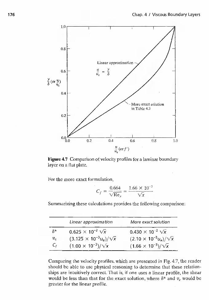
176 Chap. 4 / Viscous Boundary Layers
(or !i)
to
Figufe 4.7 Comparison of velocity profiles for a laminar boundarylayer on a flat plate.
For the more exact formulation,
0.664 1.66 x
Summarizing these calculations provides the following comparison:
Linear approximation
0.625 X
More
0.430
ex
x
act solution
Ve (3.125 X (2.10 X
Cf (1.00 x (1.66 x
Comparing the velocity profiles, which are presented in Fig. 4.7, the readershould be able to use physical reasoning to determine that these relation-ships are intuitively correct. That is, if one uses a linear profile, the shearwould be less than that for the exact solution, where 8* and Ve would begreater for the linear profile.
1
0.8
0.6
0.4
0.2 0.4 0.6 0.8
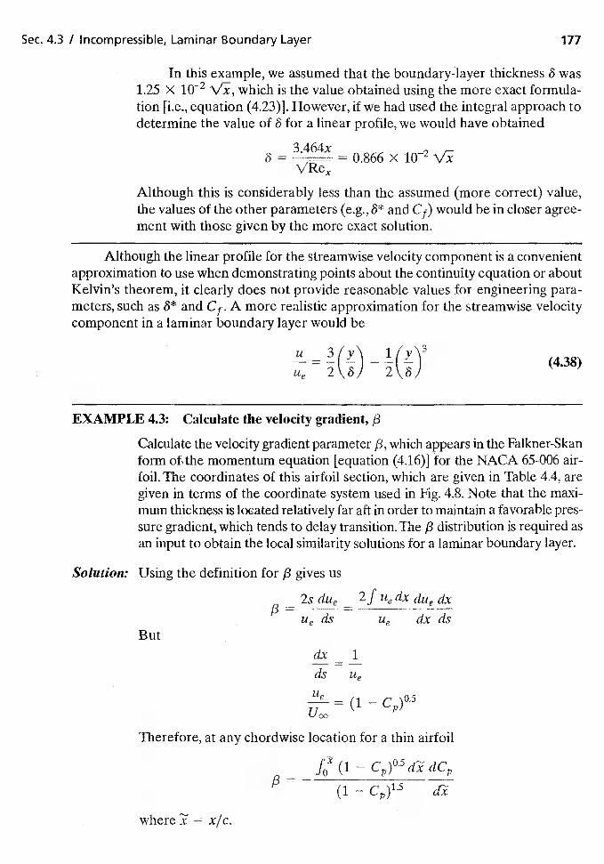
Sec. 4.3 / Jncompressible, Laminar Boundary Layer 177
In this example, we assumed that the boundary-layer thickness 6 was1.25 x 10—2 which is the value obtained using the more exact formula-tion [i.e., equation (4.23)]. However, if we had used the integral approach todetermine the value of 6 for a linear profile, we would have obtained
3.464x= 0.866 X
Although this is considerably less than the assumed (more correct) value,the values of the other parameters (e.g., 8* and Cf) would be in closer agree-ment with those given by the more exact solution.
Although the linear profile for the streamwise velocity component is a convenientapproximation to use when demonstrating points about the continuity equation or aboutKelvin's theorem, it clearly does not provide reasonable values for engineering para-meters, such as 6* and Cf. A more realistic approximation for the streamwise velocitycomponent in a laminar boundary layer would be
= 4(f)—
(4.38)
EXAMPLE 4.3: Calculate the velocity gradient, /3
Calculate the velocity gradient parameter /3, which appears in the Falkner-Skanform momentum equation [equation (4.16)] for the NACA 65-006 air-foil. The coordinates of this airfoil section, which are given in Table 4.4, aregiven in terms of the coordinate system used in Fig. 4,8. Note that the maxi-mum thickness is located relatively far aft in order to maintain a favorable pres-sure gradient, which tends to delay transition. The /3 distribution is required asan input to obtain the local similarity solutions for a laminar boundary layer.
Solution: Using the definition for /3 gives us
— 2s due — 2f tte dx due dx
— (Is — dx dsBut
dx = 1
ds
— (1 —
Therefore, at any chordwise location for a thin airfoil
— —
(1 —
where = x/c.
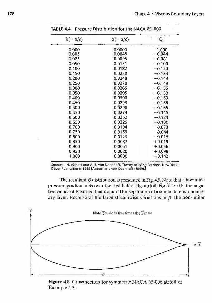
178 Chap. 4 / Viscous Boundary Layers
TABLE 4.4 Pressure Distribution for the NAcA 65--006
C,,
0.000 0.0000 1.0000.0050.025
0.00480.0096
—0.044—0.08 1
0.050 0.0131 —0.1000.100 0.0182 —0.1200.1500.2090.250
0.02480.0270
—0.134—0.143—0.149
0.300 0.0285 —0.1550.350 0.0295 —0.1590.400 0.0300 —0.1630.4500.500 0.0290
—0.166—0.165
0.550 0.0274 —0.1450.600 0.0252 —0.1240.650 —0.1000.700 0.0194 —0.0730.750 0.01 59 —0.0440.800 0.0123 —0.0130.850 +0.0190.900 0.0051 +0.0560.950 0.0020 +0.0981.000 0.0000 +0.142
Source: I. H. Abbott and A. E. von Doenhoff, Theory of Wing Sections. New York:Dover Publications, 1949 [Abbott and von Doenhoff (1949).]
The resultant /3 distribution is presented in Fig. 4.9. Note that a favorablepressure gradient acts over thO first half of the airfoil. � 0.6, the nega-tive values of /3 exceed that required for separation of a similar laminar bound-ary layer. Because of the large streamwise variations in /3, the nonsimilar
Figure 4.8 Cross section for symmetric NACA 65-006 airfoil ofExample 4.3.
x
Note is five times the
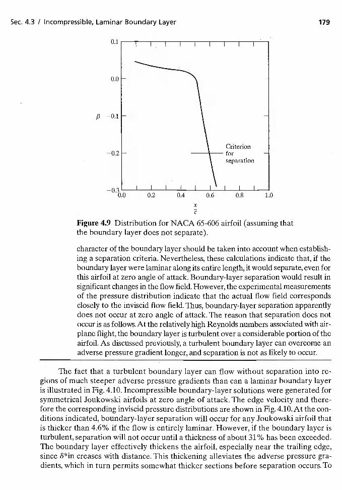
Sec. 4.3 / Incompressible, Laminar Boundary Layer 179
/3
1.0
xC
Figure 4.9 Distribution for NACA 65-606 airfoil (assuming thatthe boundary layer does not separate).
character of the boundary layer should be taken into account when establish-ing a separation criteria. Nevertheless, these calculations indicate that, if theboundary layer were laminar along its entire length, it would separate, even forthis airfoil at zero angle of attack. Boundary-layer separation would result insignificant changes in the flow field. However, the experimental measurementsof the pressure distribution indicate that the actual flow field correspondsclosely to the inviscid flow field. Thus, boundary-layer separation apparentlydoes not occur at zero angle of attack. The reason that separation does notoccur is as follows. At the relatively high Reynolds numbers associated with air-plane flight, the boundary layer is turbulent over a considerable portion of theairfoil. As discussed previously, a turbulent boundary layer can overcome anadverse pressure gradient longer, and separation is not as likely to occur.
The fact that a turbulent boundary layer can flow without separation into re-gions of much steeper adverse pressure gradients than can a laminar boundary layeris illustrated in Fig. 4.10. Incompressible boundary-layer solutions were generated forsymmetrical Joukowski airfoils at zero angle of attack. The edge velocity and there-fore the corresponding inviscid pressure distributions are shown in Fig. 4.10. At the con-ditions indicated, boundary-layer separation will occur for any Joukowski airfoil thatis thicker than 4.6% if the flow is entirely laminar. However, if the boundary layer isturbulent, separation will not occur until a thickness of about 31% has been exceeded.The boundary layer effectively thickens the airfoil, especially near the trailing edge,since creases with distance. This thickening alleviates the adverse pressure gra-dients, which in turn permits somewhat thicker sections before separation occurs. To
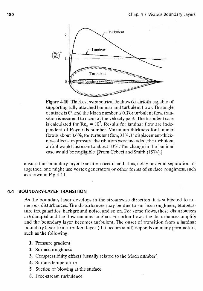
180 Chap. 4 / Vkcous Boundary Layers
2
(Ue\2
1
a
Figure 4.10 Thickest symmetrical Joukowski airfoils capable ofsupporting fully attached laminar and turbulent flows. The angleof attack is ØO, and the Mach number is 0. For turbulent flow, tran-sition is assumed to occur at the velocity peak.The turbulent caseis calculated for = 1O7. Results for laminar flow are inde-pendent of Reynolds number. Maximum thickness for laminarflow is about 4.6%,for turbulent flow, 31%. If displacement-thick-ness effects on pressure distribution were included, the turbulentairfoil would increase to about 33%. The change in the laminarcase would be negligible. [From Cebeci and Smith (1974).]
ensure that boundary-layer transition occurs and, thus, delay or avoid separation al-together, one might use vortex generators or other forms of surface roughness, suchas shown in Fig. 4.11.
4.4 BOUNDARY-LAYER TRANSITION
As the boundary layer develops in the streamwise direction, it is subjected to nu-merous disturbances. The disturbances may be due to surface roughness, tempera-ture irregularities, background noise, and so on. For some flows, these disturbancesare damped and the flow remains laminar. For other flows, the disturbances amplifyand the boundary layer becomes turbulent. The onset of transition from a laminarboundary layer to a turbulent layer (if it occurs at all) depends on many parameters,such as the following:
1. Pressure gradient2. Surface roughness3. Compressibility effects (usually related to the Mach number)4. Surface temperature5. Suction or blowing at the surface
6. Free-stream turbulence
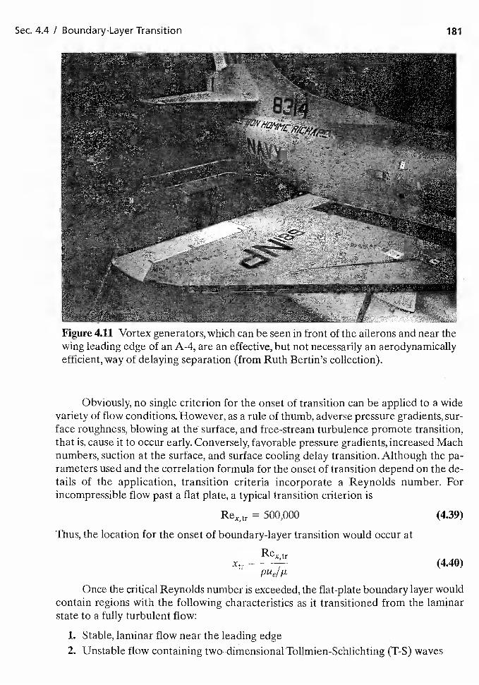
RextrXtr =
Sec. 4.4 / Boundary-Layer Transition 181
Figure 4.11 Vortex generators, which can be seen in front of the ailerons and near thewing leading edge of an A-4, are an effective, but not necessarily an aerodynamicallyefficient, way of delaying separation (from Ruth Bertin's collection).
Obviously, no single criterion for the onset of transition can be applied to a widevariety of flow conditions. However, as a rule of thumb, adverse pressure gradients, sur-face roughness, blowing at the surface, and free-stream turbulence promote transition,that is, cause it to occur early. Conversely, favorable pressure gradients, increased Machnumbers, suction at the surface, and surface cooling delay transition. Although the pa-rameters used and the correlation formula for the onset of transition depend on the de-tails of the application, transition criteria incorporate a Reynolds number. Forincompressible flow past a flat plate, a typical transition criterion is
= 500,000
Thus, the location for the onset of boundary-layer transition would occur at
(439)
(4.40)
Once the critical Reynolds number is exceeded, the flat-plate boundary layer wouldcontain regions with the following characteristics as it transitioned from the laminarstate to a fully turbulent flow:
1. Stable, laminar flow near the leading edge2. Unstable flow containing two-dimensional Tollmien-Schlichting (T-S) waves
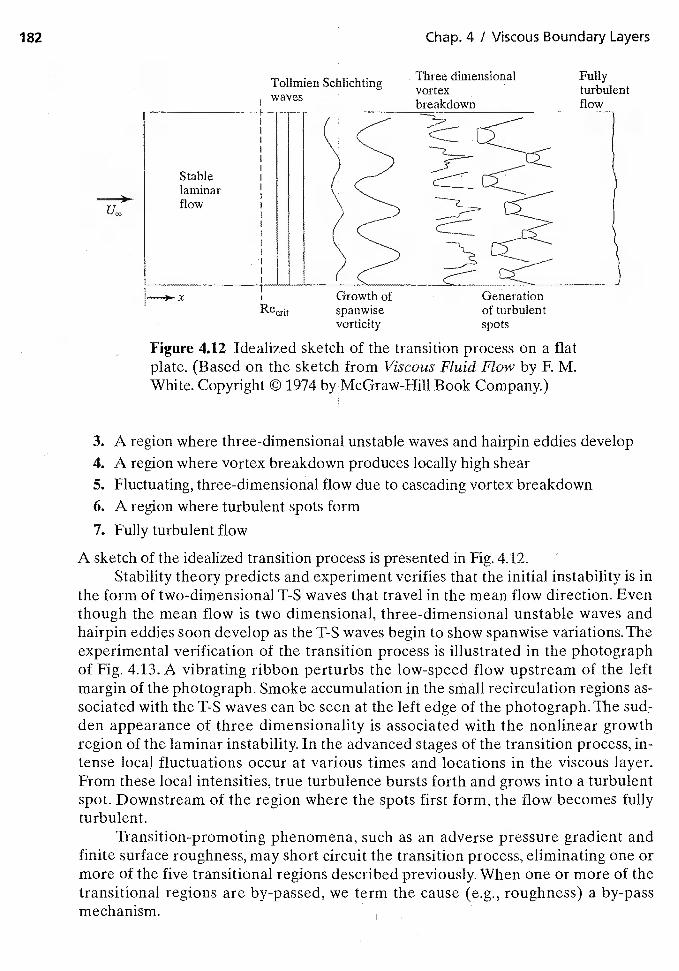
182 Chap. 4 / Viscous Boundary Layers
Figure 4.12 Idealized sketch of the transition process on a flatplate. (Based on the sketch from Viscous Fluid Flow by F. M.White. Copyright © 1974 by McGraw-Hill Book Company.)
A region where three-dimensional unstable waves and hairpin eddies developA region where vortex breakdown produces locally high shearFluctuating, three-dimensional flow due to cascading vortex breakdownA region where turbulent spots form
Fully turbulent flow
A sketch of the idealized transition process is presented in Fig. 4.12.Stability theory predicts and experiment verifies that the initial instability is in
the form of two-dimensional T-S waves that travel in the mean flow direction. Eventhough the mean flow is two dimensional, three-dimensional unstable waves andhairpin eddies soon develop as the T-S waves begin to show spanwise variations. Theexperimental verification of the transition process is illustrated in the photographof Fig. 4.13. A vibrating ribbon perturbs the low-speed flow upstream of the leftmargin of the photograph. Smoke accumulation in the small recirculation regions as-sociated with the T-S waves can be seen at the left edge of the photograph. Theden appearance of three dimensionality is associated with the nonlinear growthregion of the laminar instability. In the advanced stages of the transition process, in-tense local fluctuations occur at various times and locations in the viscous layer.From these local intensities, true turbulence bursts forth and grows into a turbulentspot. Downstream of the region where the spots first form, the flow becomes fullyturbulent.
Transition-promoting phenomena, such as an adverse pressure gradient andfinite surface roughness, may short circuit the transition process, eliminating one ormore of the five transitional regions described previously. When one or more of thetransitional regions are by-passed, we term the cause (e.g., roughness) a by-passmechanism.
Toilmien Schlichtingwaves
Three dimensionalvortexbreakdown
Fullyturbulentflow
Growth ofspanwisevorticity
Generationof turbulentspots
3.
4.
5*
6.
7.
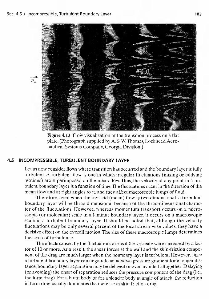
Sec. 4.5 / Incompressible, Turbu'ent Boundary Layer 183
Figure 4.13 Flow visualization of the transition process on a flatplate. (Photograph supplied by A. S. W. Thomas, Lockheed Aero-nautical Systems Company, Georgia Division.)
4.5 INCOMPRESSIBLE, TURBULENT BOUNDARY LAYER
Let us now consider flows where transition has occurred and the boundary layer is fullyturbulent. A turbulent flow is one in which irregular fluctuations (mixing or eddyingmotions) are superimposed on the mean flow. Thus, the velocity at any point in a tur-bulent boundary layer is a function of time.The fluctuations occur in the direction of themean flow and at right angles to it, and they affect macroscopic lumps of fluid.
Therefore, even when the inviscid (mean) flow is two dimensional, a turbulentboundary layer will be three dimensional because of the three-dimensional charac-ter of the fluctuations. However, whereas momentum transport occurs on a micro-scopic (or molecular) scale in a laminar boundary layer, it occurs on a macroscopicscale in a turbulent boundary layer. It should be noted that, although the velocityfluctuations may be only several percent of the local streamwise values, they have adecisive effect on the overall motion.The size of these macroscopic lumps determinesthe scale of turbulence.
The effects caused by the fluctuations are as if the viscosity were increased by a fac-tor of 10 or more. As a result, the shear forces at the wall and the skin-friction compo-nent of the drag are much larger when the boundary layer is turbulent. However, sincea turbulent boundary layer can negotiate an adverse pressure gradient for a longer dis-tance, boundary-layer separation may be delayed or even avoided altogether. Delaying(or avoiding) the onset of separation reduces the pressure component of the drag (i.e.,the form drag). For a blunt body or for a slender body at angle of attack, the reductionin form drag usually dominates the increase in skin friction drag.
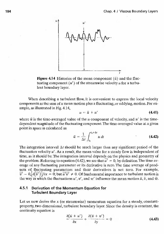
184 Chap. 4 / Viscous Boundary Layers
U
I
Figure 4.14 Histories of the mean component (n) and the fluc-tuating component (u') of the streamwise velocity ii for a turbu-lent boundary layer.
When describing a turbulent flow, it is convenient to express the local velocitycomponents as the sum of a mean motion plus a fluctuating, or eddying, motion. For ex-ample, as illustrated in Fig. 4.14,
u = + ii' (4.41)
where Li is the time-averaged value of the u component of velocity, and u' is the time-dependent magnitude of the fluctuating component. The time-averaged value at a givenpoint in space is calculated as
1udt (4.42)
The integration interval should be much larger than any significant period of thefluctuation velocity u'. As a result, the mean value for a steady flow is independent oftime, as it should be. The integration interval depends on the physics and geometry ofthe problem. Referring to equation (4.42), we see that U' = 0, by definition. The time av-erage of any fluctuating parameter or its derivative is zero. The time average of prod-ucts of fluctuating parameters and their derivatives is not zero. For example,
= 0,[a(v')]/ax 0; but u'v' 0.01 fundamental importance to turbulent motion isthe way in which the fluctuations u', v', and w' influence the mean motion ü, 13, and ü'.
4.5.1 Derivation of the Momentum Equation forTurbulent Boundary Layer
Let us now derive the x (or streamwise) momentum equation for a steady, constant-property, two-dimensional, turbulent boundary layer. Since the density is constant, thecontinuity equation is
+ u') 3(13 + v')+ 0 (4.43)
3v
Sec. 4.5 I Incompressible, Turbulent Boundary Layer 185
Expanding yieldsan au' äv'
(4.44)ax 3y ax äy
Let us take the time-averaged value for each of these terms. The first two terms alreadyare time-averaged values. As noted when discussing equation (4.42), the time-averagedvalue of a fluctuating component is zero; that is,
ax ay
Thus, for a turbulent flow, we learn from the continuity equation that
+ 0 (4.45a)ax ay
and thata' a'
(4.45b)ax 3y
Substituting the fluctuating descriptions for the velocity components into the xmomentum equation (4.6), we have
+ u') + u') du a2(u + u')p(ü + it')
ax+ P(V + v')
ay= +
ay2
Expanding gives us
_au _an an an au' au' Bu' _au'Pu— + Pv— + Pu'— + Pv'— + Pu'— + pv'— + pu— + pv—ax ay ax ay ax ax ay
dUe a2u a2u'= + +
Taking the time average of the terms in this equation, the terms that contain only onefluctuating parameter vanish, since their time-averaged value is zero. However, the timeaverage of terms involving the product of fluctuating terms is not zero. Thus, we obtain
_au _an ,au' ,au' dUe a2u(4.46)
ay ax ay dx ay
Let us now multiply the fluctuating portion of the continuity equation (4.45b) byp(i + u').We obtain
_au' au' av' av'pit— + pu'— + pü— + pu'— = 0ax ax ay ay
Taking the time average of these terms, we find that
au' av'pit'— + pu'—— 0 (4.47)
ay
186 Chap. 4 I Viscous Boundary Layers
Adding equation (4.47) to (4.46) and rearranging the terms, we obtain
due 8 2+ = + — — (4.48)
We will neglect the streamwise gradient of the time-averaged value of the square of thefluctuating velocity component, that is, (ä/äx)(u')2 as compared to the transverse gra-dient. Thus, the momentum equation becomes
a+ 0V = + — p—(u'v') (4.49)
8x 8y dx 8y
Let us further examine the last two terms,
—
(4.50)
Recall that the first term is the laminar shear stress. To evaluate the second term, let usconsider a differential area dA such that the normal to dA is parallel to the y axis, andthe directions x and z are in the plane of dA. The mass of fluid passing through this areain time dt is given by the product (pv)(dA)(dt). The flux of momentum in the x direc-tion is given by the product (u)(pv)(dA)(dt). For a constant density flow, the time-av-eraged flux of momentum per unit time is
dA = + dA
Since the flux of momentum per unit time through an area is equivalent to an equal-and-opposite force exerted on the area by the surroundings, we can treat the term —pu'v' asequivalent to a "turbulent" shear stress. This "apparent," or Reynolds; stress can beadded to the stresses associated with the mean flow. Thus, we can write
Txy = — (4.51)
Mathematically, then, the turbulent inertia terms behave as if the total stress on the sys-tem were composed of the Newtonian viscous stress plus an apparent turbulent stress.
The term —pu'v' is the source of considerable difficulties in the analysis of a tur-bulent boundary layer because its analytical form is not known a priori. It is related notonly to physical properties of the fluid but also to the local flow conditions (velocity,geometry, surface roughness, upstream history, etc.). Furthermore, the magnitude of—pu'v' depends on the distance from the wall. Because the wall is a streamline, there isno flow through it. Thus, and v' go to zero at the wall, and the flow for y isbasically laminar.
The term —pu'v' represents the turbulent transport of momentum and is knownas the turbulent shear stress or Reynolds stress. At points away from the wall, —pu'v' isthe dominant term. The determination of the turbulent shear-stress term is the criticalproblem in the analysis of turbulent shear flows. However, this new variable can be de-fined only through an understanding of the detailed turbulent structure. These termsare related not only to physical fluid properties but also to local flow conditions. Since
Sec. 4.5 / Incompressible, Turbulent Boundary Layer 187
there are no further physical laws available to evaluate these terms, empirically basedcorrelations are introduced to model them. There is a hierarchy of techniques for closure,which have been developed from models of varying degrees of rigor.
4.5.2 Approaches to Turbulence Modeling
For the flow fields of practical interest to this text, the boundary layer is usually tur-bulent. As discussed by Spalart (2000), current approaches to turbulence modeling in-clude direct numerical simulations (DNS), large-eddy simulations (LES), andReynolds-averaged Navier-Stokes (RANS).The direct numerical simulation approachattempts to resolve all scales of turbulence. Because DNS must model all scales fromthe largest to the smallest, the grid resolution requirements are very stringent and in-crease dramatically with Reynolds number. Large-eddy simulations attempt to modelthe smaller, more homogeneous scales while resolving the larger, energy containingscales, This makes LES grid requirements less stringent than those for DNS. The RANSapproach attempts to solve for the time-averaged flow, such as that described in equa-tion (4.49).This means that all scales of turbulence must be modeled. Recently, hybridapproaches that combine RANS and LES have been proposed in an attempt to com-bine the best features of these two approaches.
For the RANS approach, quantities of interest are time averaged. When this aver-aging process is applied to the Navier-Stokes equations (such as was done in Section4.5.1), the result is an equation for the mean quantities with extra term(s) involving thefluctuating quantities, the Reynolds stress tensor (e.g., Reynolds stress ten-sor takes into account the transfer of momentum by the turbulent fluctuations. It is oftenwritten that the Reynolds stress tensor is proportional to the mean strain-rate tensor[i.e., is known as the Boussinesq eddy-viscosity approximation, whereis the unknown turbulent eddy viscosity. The turbulent eddy viscosity is determined usinga turbulence model. The development of correlations in terms of known parameters is usu-ally termed as the closure problem. Closure procedures for the turbulent eddy viscosityare generally categorized by the number of partial differential equations that are solved,with zero-equation, one-equation, and two-equation models being the most popular.
Zero-equation models use no differential equations and are commonly known asalgebraic models. Zero-equation models are well adapted to simple, attached flowswhere local turbulence equilibrium exists (i.e., the local production of turbulence is bal-anced by the local dissipation of turbulence). Smith (1991) noted, "For solutions of ex-ternal flows around full aircraft configurations, algebraic turbulence models remain themost popular choice due to their simplicity." However, he further noted, "In general,while algebraic turbulence models are computationally simple, they are more difficultfor the user to apply. Since algebraic models are accurate for a narrow range of flows,different algebraic models must be applied to the different types of turbulent flows ina single flow problem. The user must define in advance which model applies to whichregion, or complex logic must be implemented to automate this process .... Differentresults can be obtained with different implementation of the same turbulence model."
By solving one or more differential equations, the transport of turbulence canbe included. That is, the effect of flow history on the turbulence can be modeled. Oneexample where modeling the flow history of turbulence is crucial is in the calculation
188 Chap. 4 / Viscous Boundary Layers
of turbulent flow over a multielement airfoil. One equation models are perhaps thesimplest way to model this effect. Wilcox (1998), when discussing the one-equationmodel of Spalart-Allmaras (1992), noted that "it is especially attractive for airfoiland wing applications, for which it has been calibrated." As a result, the Spalart-All-
• maras model, which solves a single partial differential equation for a variable that isrelated to the turbulent kinematic eddy viscosity, is one of the most popular turbu-lence models.
• In the two-equation models, one transport equation is used for the computationof the specific turbulence kinetic energy (k) and a second transport equation is used todetermine the turbulent length scale (or dissipation length scale). A variety of trans-port equations have been proposed for determining the turbulent length scale, includ-ing k-c, k-w, and k-kl models. Again, the reader is referred to Wilcox (1998) for detaileddiscussions of these models.
Smith (1991) notes," For a two equation model, the normal Reynolds stress com-ponents are assumed to be equal, while for algebraic models the normal stresses are en-tirely neglected. Experimental results show the streamwise Reynolds stress componentto be two to three times larger than the normal component. For shear flows with onlygradual variations in the streamwise direction, the Reynolds shear stress is the domi-
• nant stress term in the momentum equations and the two equation models are rea-sonably accurate. For more complex strain fields, the errors can be significant."
Neumann (1989) notes, "Turbulence models employed in computationalschemes to specify the character of turbulent flows are just that ... models, non-physical ways of describing the character of the physical situation of turbulence.The models are the result of generalizing and applying fundamental experimentalobservations; they are not governed by the physical principles of turbulence andthey are not unique."
In evaluating computations for the flow over aircraft at high angles of attack,Smith (1991) notes that "at higher angles of attack, turbulence modeling becomes moreof a factor in the accuracy of the solution." The advantage of the RANS models is thatthey are relatively cheap to compute and can provide accurate solutions to many en-gineering flows. However, RANS models lack generality. The coefficients in the vari-ous models are usually determined by matching the computations to simplebuilding-block experimental flows (e.g., zero-pressure-gradient (flat-plate) boundarylayers.) Therefore, when deciding which turbulence model to use, the user should takecare to insure that the selected turbulence model has been calibrated using measure-ments from relevant flow fields. Furthermore, the model should have sufficient accu-racy and suitable numerical efficiency for the intended applications.
For an in-depth review of turbulence models and their applications, the reader isreferred to Wilcox (1998).
4.5.3 Turbulent Boundary Layer for a Flat Plate
Since is a constant for a flat plate, the pressure gradient term is zero. Even with thissimplification, there is no exact solution for the turbulent boundary layer. Very near thewall, the viscous shear dominates. Ludwig Prandtl deduced that the mean velocity inthis region must depend on the wall shear stress, the fluid's physical properties, and the
Sec. 4.5 I Incompressible, Turbulent Boundary Layer 189
distance y from the wall. Thus, ü is a function of (Tm, p, y). To a first order, the veloc-ity profile in this region is linear; that is, ü is proportional to y. Thus,
= = (4.52)y
Let us define
= (4.53a)
andyu*
(4.53b)V
where is called the wall-friction velocity and is defined as
=(4.53c)
Note that has the form of a Reynolds number.Substituting these definitions into equation (4.52), we obtain
+*uu + ++
(y v)/u*
Introducing the definition of the wall-friction velocity, it is clear that
= (454)
for the laminar sublayer. In the laminar sublayer, the velocities are so small that viscousforces dominate and there is no turbulence. The edge of the laminar sublayer corre-sponds to a of 5 to 10.
In 1930, Theodor von Kármán deduced that, in the outer region of a turbulent bound-ary layer, the mean velocity ills reduced below the free-stream value (Ue) in a manner thatis independent of the viscosity but is dependent on the wall shear stress and the distancey over which its effect has diffused. Thus, the velocity defect (ue — Il) for the outer regionis a function of (Tm, p, y, 6). For the outer region, the velocity-defect law is given by
Ue= (4.55)
The outer region of a turbulent boundary layer contains 80 to 90% of the boundary-layerthickness 6.
In 1933, Prandtl deduced that the mean velocity in the inner region must dependon the wall shear stress, the fluid physical properties, and the distance y from the wall.Thus, Il is a function of (Tm, p, y). Specifically,
= (4.56)
for the inner region.
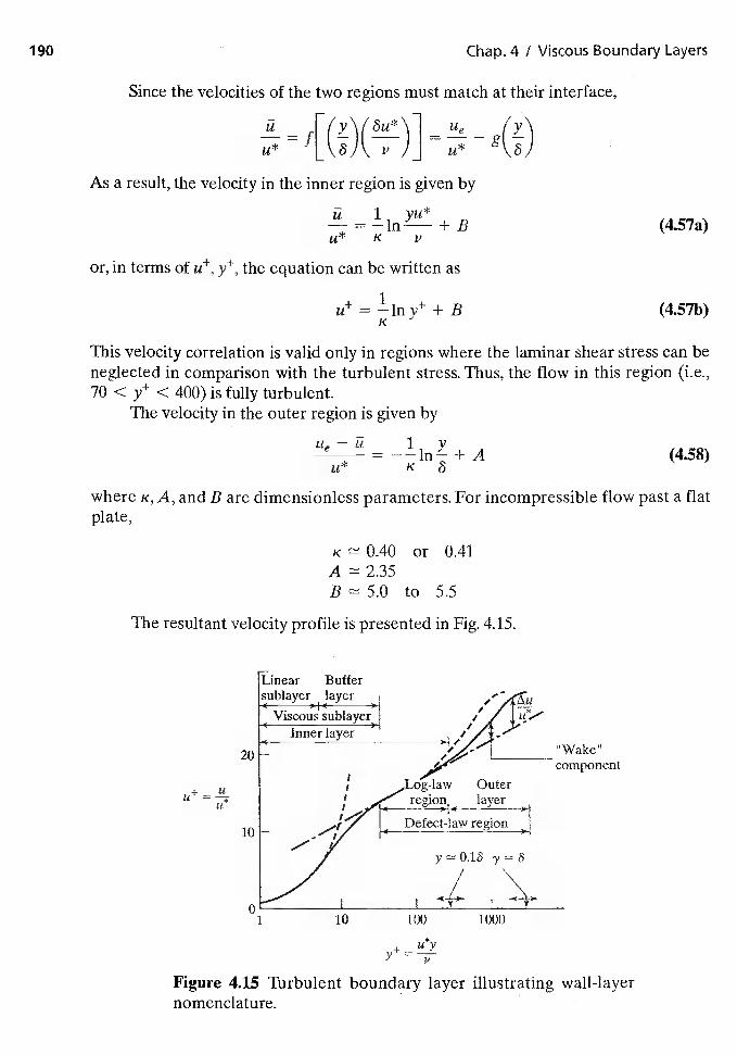
Chap. 4 I Viscous Boundary Layers
Since the velocities of the two regions must match at their interface,
U Ue (Y
As a result, the velocity in the inner region is given by
= + B (4.57a)
or, in terms of y+ the equation can be written as
= + B (4.5Th)
This velocity correlation is valid only in regions where the laminar shear stress can beneglected in comparison with the turbulent stress. Thus, the flow in this region (i.e.,70 < <400) is fully turbulent.
The velocity in the outer region is given by
Ue = —in + A (4.58)
where K, A, and B are dimensionless parameters. For incompressible flow past a flatplate,
K 0.40 or 0.41
to 5.5
The resultant velocity profile is presented in Fig. 4.15.
Linear Buffersublayer layer
Viscous sublayer I20
Inner layerWake"
/ component
÷ u g Log-law Outer= region1 layer
10 - Defect-law region
I
1 10 100 1000
+ — u*yy—p
Figure 4.15 Turbulent boundary layer illustrating wall-layernomenclature.
Sec. 4.6 / Eddy Viscosity and Mixing Length Concepts 191
The computation of the turbulent skin-friction drag for realistic aerodynamic ap-plications presents considerable challenges to the analyst, both because of grid generationconsiderations and because of the need to develop turbulence models of suitable accura-cy for the complex flow-field phenomena that may occur (e.g., viscous/inviscid interac-tions). In order to determine accurately velocity gradients near the wall, the computationalgrid should include points in the.ltiniinar sublayer. Referring to Fig. 4.15, the computa-tional grid shohid, therefore, contain points at a of 5, or less, While there are many tur-buletice models of suitable engineering accuracy available in the literature, the analystsshould calibrate the partictilar model to be used in their codes against a relevant data baseto insure that the model provides results of suitable accuracy for the applications of interest.
4.6 EDDY VISCOSITY AND MIXING LENGTH CONCEPTS
In the late nineteenth century, Boussinesq introduced the concept of eddy viscosity tomodel the Reynolds shear stress. It was assumed that the Reynolds stresses act like theviscous (laminar) shear stresses and are proportional to the transverse gradient of the(mean) streamwise velocity component. The coefficient of the proportionality is calledthe eddy viscosity and is defined as
—p=
(4.59)
Having introduced the concept of eddy viscosity, equation (4.51) for the total shearstress may be written
(au\T = T1 + Tt = + (4.60)
Like the kinematic viscosity ii, has the Units of L2/T. However, whereas v is a prop-erty of the fluid and is defined once the pressure and the temperature are known, 8mis a function of the flow field (including such factors as surface roughness, pressuregradients, etc.).
In an attempt to obtain a more generally applicable relation, Prandtl proposedthe mixing length concept, whereby the shear stress is given as
p12 (4.61)
Equating the expressions for the Reynolds stress, given by equations (4.59) and (4.61),we can now write a relation between the eddy Viscosity and the mixing length:
= (4.62)3)'
From this point on, we will use only the time-average (or mean-flow) properties. Thus,we will drop the overbar notation in the subsequent analysis.
The distributions of Cm and of 1 across the boundary layer are based on experi-mental data. Because the eddy viscosity and the mixing length concepts are based on
192 Chap. 4 / Viscous Boundary Layers
local equilibrium ideas, they provide only rough approximations to the actual flow andare said to lack generality. In fact, the original derivations included erroneous physicalarguments. However, they are relatively simple to use and provide reasonable values ofthe shear stress for many engineering applications.
A general conclusion that is drawn from the experimental evidence is that the tur-bulent boundary layer should be treated as a composite layer consisting of an inner re-gion and an outer region. For the inner region, the mixing length is given as
= Ky[(I — exp (—y/A)] (4.63)
where,< = 0.41 (as discussed earlier) and A, the van Driest damping parameter, is
A26v
(4.64a)Nu*
where is the wall friction velocity as defined by equation (4.53c)
N = (1 — (4.64b)
and
(4.64c)(u*) dx
Thus, the eddy viscosity for the inner region becomes
(Ky)2[1 - exp (4.65)
For the outer region, the eddy viscosity is given as
= aIte8* (4.66)
where is the displacement thickness as defined by equation (4.26),
0.02604a = (4.67a)1+1-I
LI 0.55[1 — exp — 0.298z1)] (4.6Th)
and
— 1 (4.67c)
where Re6 is the Reynolds number based on momentum thickness, that is, the character-istic dimension in the expression for Re0 is the momentum thickness, see equation (4.28).
The y coordinate of the interface between the inner region and the outer regionis determined by the requirement that the y distribution of the eddy viscosity be con-tinuous. Thus, the inner region expression, equation (4.65), is used to calculate the eddyviscosity until its value becomes equal to that given by the outer region expression,equation (4.66). The y coordinate, where the two expressions for the eddy viscosity areequal [i.e., when (Cm)oI,15 the interface value, y � the eddy viscos-ity is calculated using the outer region expression, equation (4.66).
Sec. 4.7 / Integral Equations for a Flat-Plate Boundary Layer 193
Recall that the transition process occurs over a finite length; that is, the boundarylayer does not instantaneously change from a laminar state to a fully turbulent profile.For most practical boundary-layer calculations, it is necessary to calculate the viscous flowalong its entire length. That is, for a given pressure distribution (inviscid flow field) andfor a given transition criterion, the boundary-layer calculation is started at the leadingedge or at the forward stagnation point of the body (where the boundary layer is lami-nar) and proceeds downstream through the transitional flow into the fully turbulent re-gion. To treat the boundary layer-in the transition zone, the expressions for the eddyviscosity are multiplied by an intermittency factor, Ytr
exp[
G(x — Xtr) (4.68a)
where Xtr is the x coordinate for the onset of transition and3
G = 8.35 X (4.68b)
The intermittency factor varies from 0 (in the laminar region and at the onset of tran-sition) to 1 (at the end of the transition zone and for fully turbulent flow). Thus, in thetransition zone,
(Ky)2[1 — exp (4.69a)
and(Sm)0 (4.69b)
Solutions have been obtained using these equations to describe the laminar, transi-tional, and turbulent boundary layer for flow past a flat plate. The results are presented inFig. 4,16,
4.7 INTEGRAL EQUATIONS FOR A FLAT-PLATEBOUNDARY LAYER
The eddy viscosity concept or one of the higher-order methods are used in developingturbulent boundary-layer solutions using the differential equations of motion. Althoughapproaches using the differential equations are most common in computational fluiddynamics, the integral approach can also be used to obtain approximate solutions for aturbulent boundary layer. Following a suggestion by Prandtl, the turbulent velocity pro-file will be represented by a power-law approximation.
We shall use the mean-flow properties in the integral form of the equation of mo-tion to develop engineering correlations for the skin-friction coefficient and the bound-ary-layer thickness for an incompressible, turbulent boundary layer on a flat plate.Since we will use only the time-averaged (or mean-flow) properties in this section, wewill drop the overbar notation. Consider the control volume shown in Fig. 4.17. Notethat the free-stream velocity of the flow approaching the plate and the velocityof the flow outside of the boundary layer adjacent to the plate (Ue) are equal and are
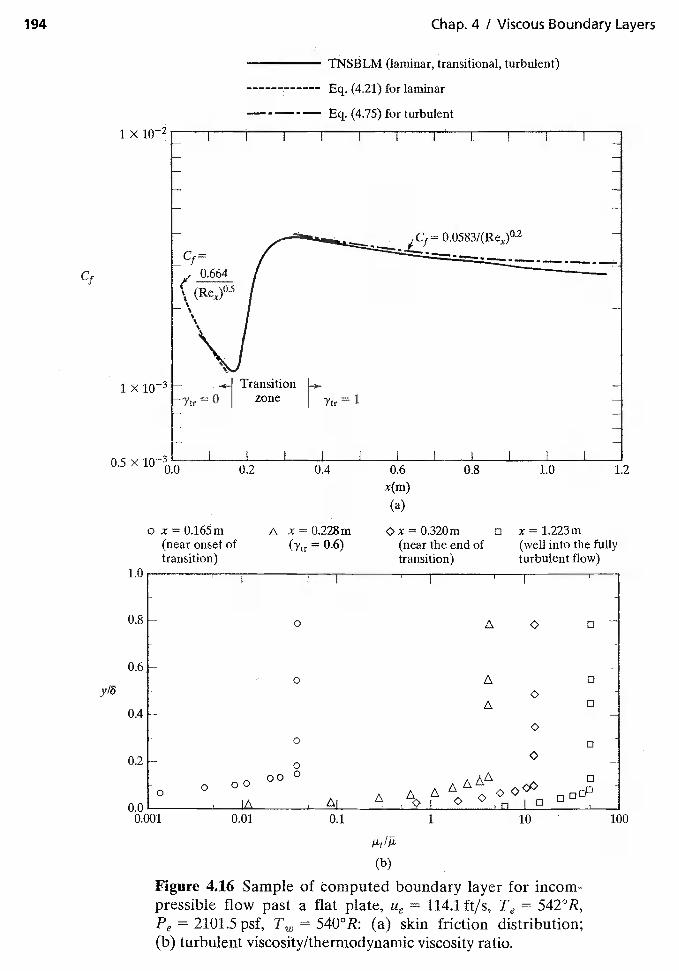
194
Cf
1 x
1 x
0.5 X
Chap. 4 / Viscous Boundary Layers
TNSBLM (laminar, transitional, turbulent)
Eq. (4.21) for laminar
— - — - — Eq. (4.75) for turbulent
0.6
x(m)
o x = 0,165m(near onset oftransition)
0,01
o x1.223m(well into the fullyturbulent flow)
(b)
Figure 4.16 Sample of computed boundary layer for incom-pressible flow past a flat plate, tie 114,1 ft/s, Te = 542°R,
= 2101.5 psI, 540°R: (a) skin friction distribution;(b) turbulent viscosity/thermodynamic viscosity ratio.
I I I I I I
Cf ==
Transition
hytrzone
0.2 0.4I I I I I I I I
0.8 1.0 1.2
(a)
x=0.228m Ox=0.320m0.6) (near the end of
transition)1.0
0.8
0.6 -
0.4 -
0.2
yrn
a00
0 Q 0
., 0 0
0
0 0
8
DO
0.1 :1 10 100
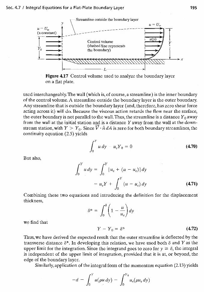
Sec. 4.7 / Integral Equations for a Flat-Plate Boundary Layer 195
x
used interchangeably. The wall (which is, of course, a streamline) is the inner boundaryof the control volume. A streamline outside the boundary layer is the outer boundary.Any streamline that is outside the boundary layer (and, therefore, has zero shear forceacting across it) will do. Because the viscous action retards the flow near the surface,the outer boundary is not parallel to the wall. Thus, the streamline is a distance Y0 awayfrom the wall at the initial station and is a distance Y away from the wall at the down-stream station, with Y > Y0. Since V. Fl dA is zero for both boundary streamlines, thecontinuity equation (2.5) yields
I u dy UeY0 = 0 (4.70)Jo
But also,
J udYJ [Ue+(uue)]dy0. 0
p1'= UeY + I (u — lie) dy (4.71)
Jo
Combining these two equations and introducing the definition for the displacementthickness,
= —
we find thaty — = (4.72)
Thus, we have derived the expected result that the outer streamline is deflected by thetransverse distance In developing this relation, we have used both 6 and Y as theupper limit for the integration. Since the integrand goes to zero for y � 6, the integralis independent of the upper limit of integration, provided that it is at, or beyond, theedge of the boundary layer.
Similarly, application of the integral form of the momentum equation (2.13) yields
ry rYo
—d= / u(pudy) — IJo Jo
Figure 4.17 Control volume used to analyze the boundary layeron a flat plate.
196 Chap. 4 1 Viscous Boundary Layers
Note that the lowercase letter designates the drag per unit span (d). Thus,ry
d = — I (pu2 dy) (4.73)Jo
Using equation (4.70), we find that1Y
d PUe I udy — I pu2dyJO Jo
This equation can be rewritten in terms of the section drag coefficient as
dCd=
/ 22 u u= —( / —dy
— J(4.74)L\Jo Ue 0
Recall that the momentum thickness for an incompressible flow is
=(1
-dy (4.28)
Ue
Note that the result is independent of the upper limit of integration provided that theupper limit is equal to or greater than the boundary-layer thickness. Thus, the drag co-efficient (for one side of a flat plate of length L) is
Cd = (4.75)
The equations developed in this section are valid for incompressible flow past a flatplate whether the boundary layer is laminar or turbulent.The value of the integral tech-nique is that it requires only a "reasonable" approximation for the velocity profile [i.e.,u(y)} in order to achieve "fairly accurate" drag predictions, because the integration oftenaverages out positive and negative deviations in the assumed velocity function.
4.7.1 Application of the Integral Equations of Motion toa Turbulent, Flat-Plate Boundary Layer
Now let us apply these equations to develop correlations for a turbulent boundary layeron a flat plate. As discussed earlier, an analytical form for the turbulent shear is not knowna priori. Therefore, we need some experimental information. Experimental measure-ments have shown that the time-averaged velocity may be represented by the power law,
u—=(—) (4.76)Ue \6J
when the local Reynolds number Re,, is in the range 5 x 1 x i07. However, notethat the velocity gradient for this profile,
t3UUe 1 1
ay — 7 6l/7y6/7
Sec. &7 / Integral Equations for a Flat-Plate Boundary Layer 197
goes to infinity at the wall. Thus, although the correlation given in equation (4.76) pro-vides a reasonable representation of the actual velocity profile, we need another pieceof experimental data: a correlation for the shear at the wall. Blasius found that the skinfriction coefficient for a turbulent boundary layer on a flat plate where the local Reynoldsnumber is in the range 5 X i05 to 1 X i07 is given by
7Cf = 1 2
0.0456(1
(4.77)\Ue81
Differentiating equation (4.69) gives us
= (4.78)dx Ue 8
Substituting equations (4.76) and (4.77) into equation (4.78), we obtain
=fl - (x)hhl]d(x)}
which becomes/ \o.25
6°25d6 0.23451 dx,J
If we assume that the boundary-layer thickness is zero when x = 0, we find that
8 =
Rearranging, the thickness of a turbulent boundary layer on a flat plate is given by
8 — 0.3747
x (Rex)
Comparing the turbulent correlation given by equation (4.79) with the laminarcorrelation given by equation (4.23), we see that a turbulent boundary layer grows at afaster rate than a laminar boundary layer subject to the same conditions. Furthermore,at a given x station, a turbulent boundary layer is thicker than a laminar boundary layerfor the same stream conditions.
Substitution of equation (4.79) into equation (4.77) yields
= 0.0583(4.80)
As with the laminar skin-friction coefficient found in Sec. 4.3.1, a total skin-frictioncoefficient can be found for turbulent flow by integrating equation (4.80) over the lengthof a flat plate:
— 1 11L
0.0583Cf = I C1 (x)dx = I dxU0 U0
= 0.074(4.81)' (ReL)°2
Chap. 4 I Viscous Boundary Layers
This formula, known as the Prandtl formula, is an exact theoretical representation of theturbulent skin-friction drag. However, when compared with experimental data, it isfound to be only ±25% accurate. A number of other empirical and semi-empirical tur-bulent skin-friction coefficient relations also have been developed, some of which areconsiderably more accurate than the Prandtl formula [White (2005)1:
Prandtl-Schlichting:
C ±3% accurate (4.82)(log10 Rei )2.58
Karman-Schoenherr:
4.13 log18 (ReL ±2% accurate (4.83)VCf
Schultz-Grunow:
— 0,427Cf ±7% accurate (4.84)
(log10 ReL — 0.407)2.64
While the Karman-Schoenherr relation is the most accurate of these relationships, it re-quires an iterative solution method to obtain a result, since the drag coefficient is not ex-plicitly represented. Therefore, the most accurate relation which is also straight-forwardto use is the Prandtl-Schlichting relation, which should usually be used instead of thePrandtl theoretical relation, equation (4.81).
The calculation of the skin-friction drag for a flat plate with transition theoreticallywould require using the local skin-friction coefficients, equation (4.21) for the laminarportion of the flow and equation (4.80) for the turbulent part of the care toonly integrate each relation over the laminar and turbulent lengths, respectively.
111'tr )CD = / Cf1 dx + / C1
bdx (4.85)
)
Another approach is to use the total skin-friction coefficients, which are equation (4.32)for the laminar portion of the flow and equation (4.82) for the turbulent part of the flow. Caremust be taken, however, when using the total skin-friction coefficients, since they already rep-resent the integrated skin friction over the entire plate from x = 0 to x = L. In order toproperly simulate a flat plate with transitional flow present, the process shown in Fig. 4.18should be used. Since you want to simulate the plate with both laminar and turbulent bound-ary layers present, you start by evaluating the entire plate by assuming that the boundarylayer is turbulent along the entire length of the plate. Since the distance from the leading edgeof the plate to the transition location should be evaluated with laminar flow, that portion ofthe plate should be evaluated with the turbulent-flow skin-friction relation and also with thelaminar-flow skin-friction relation by subtracting the turbulent-flow drag from the total plateturbulent results and adding the laminar-flow portion. In equation form, this would be:
— Lb — — XtrbCD = — + (4.86)
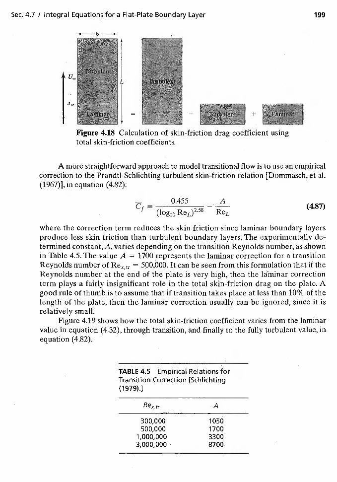
Sec. 4.7 / integral Equations for a Flat-Plate Boundary Layer 199
— 0.455 Acf=_
(log10 ReL
TABLE 4.5 EmpiricalTransition COrrection
Relations for[Sch I ichti ng
(1979).]
Rextr A
300,000 1050500,000 1700
1,000,000 33003,000,000 8700
b
+
Figure 4.18 Calculation of skin-friction drag coefficient usingtotal skin-friction coefficients.
A more straightforward approach to model transitional flow is to use an empiricalcorrection to the Prándtl-Schlichting turbulent skin-friction relation [Dommasch, et a!.(1967)], in equation (4.82):
(4.87)
where the correction term reduces the skin friction since laminar boundary layersproduce less skin friction than turbulent boundary layers. The experimentally de-termined constant,A, varies depending on the transition Reynolds number, as shownin Table 4.5. The value A = 1700 represents the laminar correction for a transitionReynolds number of Rextr = 500,000. It can be seen from this formulation that if theReynolds number at the end of the plate is very high, then the laTminar correctionterm plays a fairly insignificant role in the total skin-friction drag on the plate. Agood rule of thumb is to assume that if transition takes place at less than 10% of thelength of the plate, then the laminar correction usually can be ignored, since it isrelatively small.
Figure 4.19 shows how the total skin-friction coefficient varies from the laminarvalue in equation (4.32), through transition, and finally to the fully turbulent value, inequation (4.82).
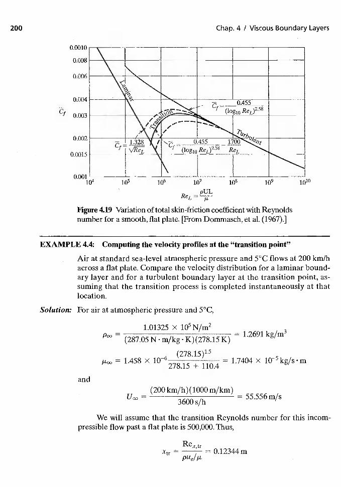
200 Chap. 4 / Viscous Boundary Layers
Cf
Figure 4.19 Variation of total skin-friction coefficient with Reynoldsnumber for a smooth, flat plate. [From Dommasch, et al. (1967).]
EXAMPLE 4.4: Computing the velocity profiles at the "transition point"
Air at standard sea-level atmospheric pressure and 5°C flows at 200 km/hacross a flat plate. Compare the velocity distribution for a laminar bound-ary layer and for a turbulent boundary layer at the transition point, as-suming that the transition process is completed instantaneously at thatlocation.
Solution: For air at atmospheric pressure and 5°C,
and
1.01325 X N/rn2
== 1.2691 kg/rn3
(278.15)1.5= 1.458 x 10627815 + 110.4
= 1.7404 X
tr= 0.12344m
0.001106
pULReL =
108 1010
(200 km/h) (1000 m/km)UOO
= 3600s/h= 55.556 rn/s
We will assume that the transition Reynolds number for this incom-pressible flow past a flat plate is 500,000. Thus,
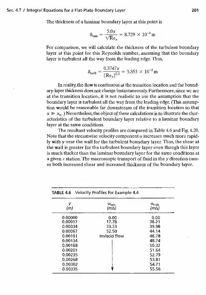
Sec. 4.7 / Integral Equations for a Flat-Plate Boundary Layer 201
The thickness of a laminar boundary layer at this point is
5.Ox 4= 8.729 x mv
For comparison, we will calculate the thickness of the turbulent boundarylayer at this point for this Reynolds number, assuming that the boundarylayer is turbulent all the way from the leading edge. Thus,
8turb0.374
= 3.353 x m
In reality, the flow is continuous at the transition location and the bound-ary-layer thickness does not change instantaneously. Furthermore, since we areat the transition location, it is not realistic to use the assumption that theboundary layer is turbulent all the way from the leading edge. (This assump-tion would be reasonable far downstream of the transition location so thatx Nevertheless, the object of these calculations is to illustrate the char-acteristics of the turbulent boundary layer relative to a laminar boundarylayer at the same conditions.
The resultant velocity profiles are compared in Table 4.6 and Fig. 4.20.Note that the streamwise velocity component u increases much more rapid-ly with y near the wall for the turbulent boundary layer. Thus, the shear atthe wall is greater for the turbulent boundary layer even though this layeris much thicker than the laminar boundary layer for the same conditions ata given x station. The macroscopic transport of fluid in the y direction caus-es both increased shear and increased thickness of the boundary layer.
TABLE 4.6 Velocity Profiles for Example 4.4
V(m) (mis)
Uturb(mis)
0.00000 0.00 0.000.00017 17.78 36.210.00034 33.33 39.980.00067 52.50 44.140.00101 Inviscid flow 46.780.00134 48.740.00168 50.320.00201 51.640.00235 52.790.00268 53.810.00302 54.710.00335 55.56
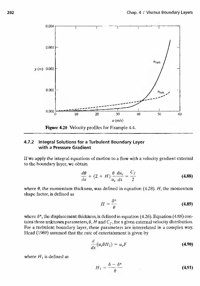
dx Ue dx 2
6*H=—0
H1 = 6 3*(4.91)
202 Chap. 4 / Viscous Boundary Layers
0.004
0.003
y(m) 0.002
0.001
0.000
u (mis)
Figure 4.20 Velocity profiles for Example 4.4.
10 20 30 40 50 60
4.7.2 Integral Solutions for a Turbulent Boundary Layerwith a Pressure Gradient
If we apply the integral equations of motion to a flow with a velocity gradient externalto the boundary layer, we obtain
(4.88)
where 8, the momentum thickness, was defined in equation (4.28). H, the momentumshape factor, is defined as
(4.89)
where 8*, the displacement thickness, is defined in equation (4.26). Equation (4.88) con-tains three unknown parameters, 0, H and Cf, for a given external velocity distribution.For a turbulent boundary layer, these parameters are interrelated in a complex way.Head (1969) assumed that the rate of entertainment is given by
where H1 is defined as
(4.90)
Sec. 4.8 I Thermal Boundary Layer for Constant-Property Flows 203
Head also assumed that H1 is a function of the shape factor H, that is, H1 = G(H). Cor-relations of several sets of experimental data that were developed by Cebeci and Brad-shaw (1979) yielded
F = 0.0306(H1 — 30)_06169 (4.92)
and
G — J0.8234(H — + 3.3 forH 1.6
—— O.6778)_3.0M + 3.3 forH � 1.6
Equations (4.90) through (4.93) provide a relationship between 0 and H. A rela-tion between Cf, 0, and H is needed to complete our system of equations. A curvefitformula given in White (2005) is
Cf= (log
(4.94)
where Re0 is the Reynolds number based on the momentum thickness:
Re9 = (4.95)
We can numerically solve this system of equations for a given inviscid flow field.To start the calculations at some initial streamwise station, such as the transition loca-tion, values for two of the three parameters, 0, H, and Cf, must be specified at this sta-tion.The third parameter is then calculated using equation (4.94). Using this method, theshape factor H can be used as a criterion for separation. Although it is not possible todefine an exact value of H corresponding to the separation, the value of H for separa-tion is usually in the range 1.8 to 2.8.
4.8 THERMAL BOUNDARY LAYER FOR CONSTANT-PROPERTY FLOWS
As noted earlier, there are many constant-property flows for which we are interested incalculating the convective heat transfer. Thus, the temperature variations in the flowfield are sufficiently large that there is heat transfer to or from a body in the flow butare small enough that the corresponding variations in density and viscosity can be ne-glected. Let us examine one such flow, the thermal boundary layer for a steady, low-speed flow past a flat plate. We will consider flows where the boundary layer is laminar.The solution for the velocity field for this flow has been described earlier in this chap-ter; see equations (4.6) through (4.27).
We will now solve the energy equation (2.32), in order to determine the temper-ature distribution. For a low-speed, constant-property, laminar boundary layer, the vis-cous dissipation is negligible (i.e., 4 = 0). For flow past a flat plate, dp/dt = 0. Thus, fora calorically perfect gas, which will be defined in Chapter 8, equation (2.32) becomes
aT 32T+ = (4,96)
204 Chap. 4 / VIscous Boundary Layers
Note that we have already neglected k(82T/8x2) since it is small compared to k(32T/3y2).We made a similar assumption about the corresponding velocity gradients when workingwith the momentum equation; see equation (4.6).
Let us now change the dependent variable from T to the dimensionless parame-ter 0, where
TeTwNote that 0 = 0 at the wall (i.e., at y = 0), and 0 1 at the edge of the thermal boundarylayer. Using 0 as the dependent variable, the energy equation becomes
80 80 k820pu — + pv— = (4.97)
8x 8y Ce 8y2
Since the pressure is constant along the flat plate, the velocity at the edge of theboundary layer (Ue) is constant, and the momentum equation becomes
82upu— + pv— (4.98)
3y
Let us replace u in the derivatives by the dimensionless parameter, where
U= —
Thus, equation (4.98) becomes
02u*+ pv— = (4.99)
Note that 0 at the wall (i.e., at y = 0), and 1 at the edge of the velocityboundary layer.
Compare equations (4.97) and (4.98). Note that the equations are identical ifk/cr = Furthermore, the boundary conditions are identical: 0 = 0 and = 0 at thewall, and 0 = 1 and = 1 at the edge of the boundary layer. Thus, if
k
the velocity and the thermal boundary layers are identical. This ratio is called the Prandtlnumber (Pr) in honor of the German scientist:
j-tCPr = (4.100)
The Prandtl number is an important dimensionless parameter for problems involving con-vective heat transfer where one encounters both fluid motion and heat conduction.
Sec. 4.8 / Thermal Boundary Layer for Constant-Property Flows 205
4.8.1 Reynolds Analogy
The shear at the wall is defined as
IT/L\ ay
Therefore, the skin-friction coefficient for a flat plate is
— T 2,Läu*— 1 2 = (4.101)
The rate at which heat is transferred to the surface is defined as
= (4.102)y=o
The Stanton number (designated by the symbols St or C,1), which is a dimensionlessheat-transfer coefficient, is defined as
St Ch = (4.103)PLteCp(Te T20)
Combining these last two expressions, we find that the Stanton number is
St = (4.104)PUeCp ay
Relating the Stanton number, as given by equation (4.104), tO the skin-frictioncoefficient, as defined by equation (4.101), we obtain the ratio
Cf au*/ay= (4.105)
St k ao/ay
Note that if = Pr = 1, then
— 80
3y
Thus, if the Prandtl number is 1,
C
2(4.106)
This relation between the heat-transfer coefficient and the skin-friction coefficient isknown as the Reynolds analogy.
206 Chap. 4 / Viscous Boundary Layers
EXAMPLE 4.5: Calculating the thermal properties of air
The thermal conductivity of air can be calculated using the relation
k = 4.76 X 10⁶T +112cal/cm s K (4.107)
over the range of temperatures below those for which oxygen dissociates,that is, approximately 2000 K at atmospheric pressure. What is the Prandtlnumber for air at 15°C, that is, at 288.15 K?
Solution: Using the results from Example 1.3, the viscosity is 1.7894 X kg/s m.The specific heat is 1004.7 J/kg K. Using the equation to calculate the ther-mal conductivity,
(288.15)15k = 4.76 X
400.15= 5.819 X 10⁵ca1/cmsK
Noting that there are 4.187 J/cal, the thermal conductivity is
k = 2.436 X
Thus,
= = (1.7894 X 10⁵kg/s.m)(1004.7J/kg.K)= 0.738
k 2.436 >< 102J/m•s•K
Note that, as a rule of thumb, the Prandtl number for air is essentially con-stant (approximately 0.7) over a wide range of flow conditions.
4.8.2 Thermal Boundary Layer for Pr 1
To solve for the temperature distribution for the laminar, flat-plate boundary layer, letus introduce the transformation of equation (4.10):
Using the transformed stream function f, as defined by equation (4.13), equation (4.85)becomes
+ (Pr)fO' = 0 (4.108a)
where the ' denotes differentiation with respect to 17. But we have already obtainedthe solution for the stream function. Referring to equation (4.16) for a flat plate (i.e.,13 = 0),we have
'F,
f = — (4.108b)
Sec. 4.8 / Thermal Boundary Layer for Constant-Property Flows 207
Combining equations (4.108a) and (4.108b) and rearranging, we obtain
Integrating twice yields
8 = C f (fll)Prd + (4.109)
where C and 0o are constant of integration. They can be evaluated by applying the bound-ary conditions (1) at = 0,0 = 0, and (2) for large, 0 1.
00 ,, Prj (f)8 = = 1— (4.110)TeTw fOo(flP)Prdfl
The rate at which heat is transferred to the wall can be calculated using
= = k(Te —• ay
Using the values of Pohihausen, we find that
= 0.4696(Pr)°333
Combining these two relations, the rate at which heat is transferred from a laminarboundary layer to the wall is given by the relation
O.332k(Te — (4.111)
The heat transfer can be expressed in terms of the Stanton number using equation(4.103). Thus,
St =/LCp PUeX
Using the definitions for the Reynolds number and Prandtl number, the Stantonnumber is
0.332St = • (4.112)
Another popular dimensionless heat-transfer parameter is the Nusselt number.The Nusselt number is defined as
(4.113a)
In this equation, Ii is the local heat-transfer coefficient, which is defined as
hTe
(4.113h)
208 Chap. 4 / Viscous Boundary Layers
Combining this definition with equation (4.111) and (4J13a) gives us
= (Pr)°333 (4.114)
By dividing the expression for the Stanton number, equation (4.112), by that for theskin-friction coefficient, equation (4,21), we obtain
CfSt
2(Pr)°667(4.115)
Because of the similarity between this equation and equation (4.106), we shall call thisthe modified Reynolds analogy.
EXAMPLE 4.6: Calculating the heat-transfer rate for a turbulentboundary layer on a flat plate
Using the modified Reynolds analogy, develop relations for the dimensionlessheat-transfer parameters, St and for a turbulent flat-plate boundary layer.
Solution: Referring to the discussion of turbulent boundary layers, we note that
C0.0583
(4.80)
Thus, using equation (4.115) for the mOdified Reynolds analogy, we canapproximate the Stanton number as
0. 0292St = (4.116)
Comparing equations (4.112) and (4.114), we can see that the is given as
=
Thus, the Nusselt number for turbulent flow past a flat plate can be approx-imated as
(4.117)
EXAMPLE 4.7: Calculating the heat transfer
The radiator systems on many of the early racing aircraft were flush mountedon the external surface of the airplane. Let us assume that the local heat-transfer rate can be estimated using the flat-plate relations. What is the localheating rate for x = 3.0 m when the airplane is flying at 468 km/h at analtitude of 3 km? The surface temperature is 330 K.
Solution: Using Table 1.2 to find the free-stream flow properties,
= 7.012 X N/rn2 = 268.659 K
= 0.9092 kg/rn3 = 1.6938 X kg/s 'm
Sec. 4.8 / Thermal Boundary Layer for Constant-Property Flows 209
Since we have assumed that the flow corresponds to that for a flat plate,these values are also the local properties at the edge of the boundary layerat x = 3.0m. Note that
Ue = = 468 km/h = 130 rn/s
To determine whether the boundary layer is laminar or turbulent, letus calculate the local Reynolds number:
= PeUeX = (0.9092)(130)(3.O)= 2.093 x i07
1.6938 X
This is well above the transition value. In fact, if the transition Reynoldsnumber is assumed to be 500,000, transition would occur at a point
500,000Xtr 0,072 m
from the leading edge. Thus, the calculation of the heating will be based onthe assumption that the boundary layer is turbulent over its entire length.
Combining equations (4.113a) and (4.113b),
NUxk(Te
where the is given by equation (4.117).Thus,
0.0292(Rex)°'8(Pr)°'333k(Te —q=x
To calculate the thermal conductivity for air,
Ti.5k 4.76 X 10*6 = 5.506 X cal/cm s KT+112
= 2.306 X 10²J/msKSince 1 W 1 J/s,
k = 2.306 x 10⁻² W/m ' K
Furthermore, the Prandtl number is
Pr = 0.738
Thus,
(0.0292)(2.093 X 10⁷)0.8(0.738)0.333(2.306 X 10²W/mK)(268.659 — 330)K
3.Om
= —8.944 X i03 W/m2 = —8.944 kW/m2
The minus sign indicates that heat is transferred from the surface to the airflowing past the aircraft. This is as it should be, since the surface is hotterthan the adjacent air. Furthermore, since the problem discusses a radiator,proper performance would produce cooling. Since there are 1.341 hp/kW,the heat transfer rate is equivalent to 1.114 hp/ft2.
210 Chap. 4 / Viscous Boundary Layers
4.9 SUMMARY
In this chapter we have developed techniques by which we can obtain solutions for a thin,viscous boundary layer near the surface. Techniques have been developed both for alaminar and for a turbulent boundary layer using both integral and differential ap-proaches. We now have reviewed the basic concepts of fluid mechanics in Chapters 1through 4 and are ready to apply them to aerodynamic problems.
PROBLEMS
4.1. A very thin, "flat-plate" wing of a model airplane moves through the air at standard sea-levelconditions at a velocity of 15 m/s. The dimensions of the plate are such that its chord (stream-wise dimension) is 0.5 m and its span (length perpendicular to the flow direction) is 5 m.Whatis the Reynolds number at the trailing edge (x = 0.5 m)? Assume that the boundary layeris laminar in answering the remaining questions. What are the boundary-layer thicknessand the displacement thickness at the trailing edge? What are the local shear at the wall andthe skin-friction coefficient at x = 0.5 m? Calculate the total drag on the wing (both sides).Prepare a graph of It as a function of y, where It designates the x component of velocityrelative to a point on the ground, at x = 0.5 m.
4.2. Assume that the inviscid external flow over a configuration is given by
ue = Ax
Thus, the stagnation point occurs at the leading edge of the configuration (i.e., at x =0).Obtain the expression for /3. Using Fig. 4.4 and assuming that the boundary layer is lami-nar, determine the value of f"(O), that is, the value of the shear function at the wall. Whatis the relation between the shear at a given value of x this flow and that for a flat plate?
4.3. Consider two-dimensional, incompressible flow over a cylinder, For ease of use with thenomenclature of the current chapter, we will assume that the windward plane of symmetry(i.e., the stagnation point) is 6 0 and that 6 increases in the streamwise direction. Thus,
Ue = sin 6 and x = RO
Determine the values of /3, at 0 = 30°, at 0 = 45°, and at 6 = 90°.
4.4. Assume that the wall is porous so that there can be flow through the wall; that is,v(x, 0) = 0. Using equation (4.14), show that
— f(°)
in order to have similarity solutions; that is, = 0 for steady, incompressible flowpast a flat plate,
4.5. We plan to use suction through a porous wall as a means of boundary-layer control. Usingthe equation developed in Problem 4.4, determine f(0) if = for steady flowpast a flat plate where tie = 10 rn/s at standard sea-level conditions. What are the remain-ing two boundary conditions?
4.6. Transpiration (or injecting gas through a porous wall into the boundary layer) is to be usedto reduce the skin-friction drag for steady, laminar flow past a flat plate. Using the equationdeveloped in Problem 4.4, determine if f(0) = —0.25. The inviscid velocity (Ue) is 50ft/s with standard atmospheric conditions.
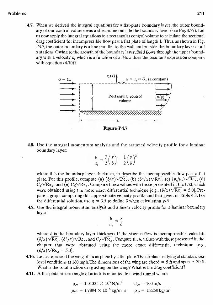
Problems
4.7. When we derived the integral equations for a flat-plate boundary layer, the outer bound-ary of our control volume was a streamline outside the boundary layer (see Fig. 4.17). Letus now apply the integral equations to a rectangular control volume to calculate the sectionaldrag coefficient for incompressible flow past a flat plate of length L. Thus, as shown in Fig.P4.7, the outer boundary is a line parallel to the wall and outside the boundary layer at allx stations. Owing to the growth of the boundary layer, fluid flows through the upper bound-ary with a velocity Ve which is a function of x, How does the resultant expression comparewith equation (4.70)?
U Uc,,
4.8. Use the integral momentum analysis and the assumed velocity profile for a laminarboundary layer:
u 3(y'\ 1(y'\32U)
where 8 is the boundary-layer thickness, to describe the incompressible flow past a flatplate. For this profile, compute (a) (b) (c) (d)
and (e) Compare these values with those presented in the text, whichwere obtained using the more exact differential technique [e.g., = 5.0]. Pre-pare a graph comparing this approximate velocity profile and that given in Table 4.3. Forthe differential solution, use 7) = 3.5 to define 6 when calculating y/6.
4.9. Use the integral momentum analysis and a linear velocity profile for a laminar boundarylayer
U _YUe6
where 8 is the boundary layer thickness. If the viscous flow is incompressible, calculate(8*/x) and Compare these values with those presented in the
chapter that were obtained using the more exact differential technique [e.g.,= 5.0].
4.10. Let us represent the wing of an airplane by a flat plate. The airplane is flying at standard sea-level conditions at 180 mph.The dimensions of the wing are chord = 5 ft and span = 30 ft.What is the total friction drag acting on the wing? What is the drag coefficient?
4.11. A fiat plate at zero angle of attack is mounted in a wind tunnel where
= 1.01325 x N/rn2 = 100 m/s
= 1.7894 X kg/rn s = 1.2250 kg/rn3
U = Ue = (a constant)
Figure P4.7
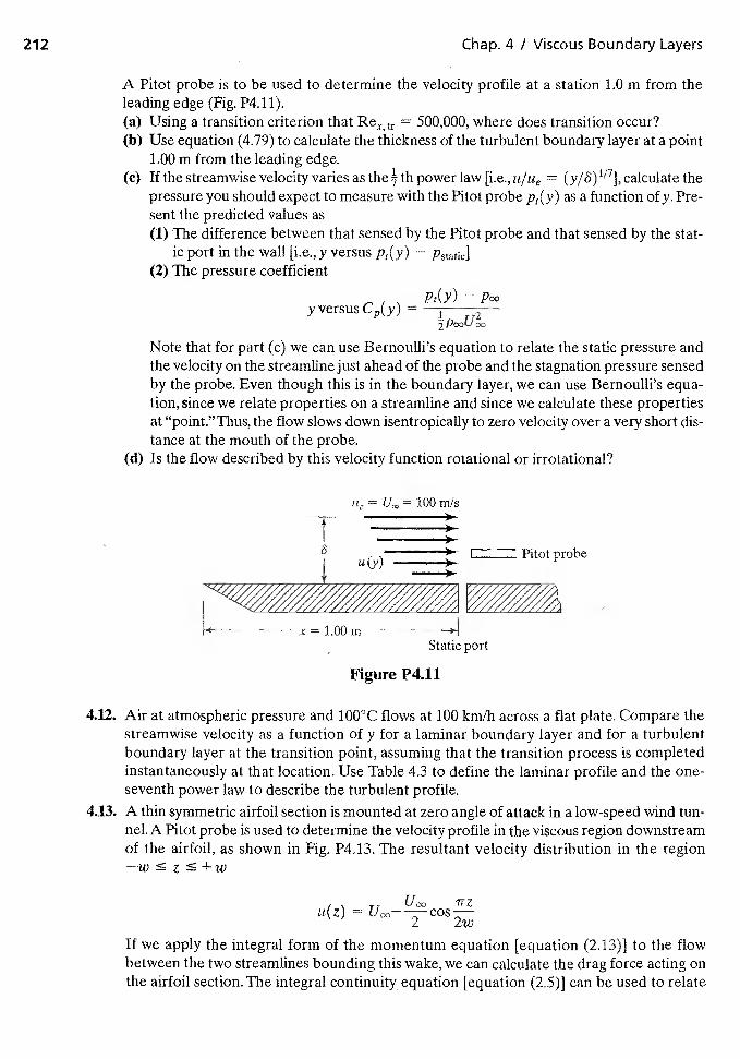
212 Chap. 4 / Viscous Boundary Layers
A Pitot probe is to be used to determine the velocity profile at a station 1.0 m from theleading edge (Fig. P4.11).(a) Using a transition criterion that = 500,000, where does transition occur?(b) Use equation (4.79) to calculate the thickness of the turbulent boundary layer at a point
1.00 m from the leading edge.(c) If the streamwise velocity varies as the th power law [i.e., u/Ue = (y/6)117], calculate the
pressure you should expect to measure with the Pitot probe Pt(Y) as a function of y. Pre-sent the predicted values as(1) The difference between that sensed by the Pitot probe and that sensed by the stat-
ic port in the wall [i.e.,y versus Pt(Y) — pstatic](2) The pressure coefficient
Pt(Y) —1
Note that for part (c) we can use Bernoulli's equation to relate the static pressure andthe velocity on the streamline just ahead of the probe and the stagnation pressure sensedby the probe. Even though this is in the boundary layer, we can use Bernoulli's equa-tion, since we relate properties on a streamline and since we calculate these propertiesat "point." Thus, the flow slows down isentropically to zero velocity over a very short dis-tance at the mouth of the probe.
(d) Is the flow described by this velocity function rotational or irrotational?
= = 100 rn/S
__
I Pitot probeu(y)I—
x=1.OOrnStatic port
Figure P4.11
4.12. Air at atmospheric pressure and 100° C flows at 100 km/h across a flat plate. Compare thestreamwise velocity as a function of y for a laminar boundary layer and for a turbulentboundary layer at the transition point, assuming that the transition process is completedinstantaneously at that location. Use Table 4.3 to define the laminar profile and the one-seventh power law to describe the turbulent profile.
4.13. A thin symmetric airfoil section is mounted at zero angle of attack in a low-speed wind tun-nel. A Pitot probe is used to determine the velocity profile in the viscous region downstreamof the airfoil, as shown in Fig. P4.13. The resultant velocity distribution in the region—w � z +w
Uc,ou(z) =
If we apply the integral form of the momentum equation [equation (2.13)1 to the flowbetween the two streamlines bounding this wake, we can calculate the drag force acting onthe airfoil section. The integral continuity equation [equation (2.5)] can be used to relate
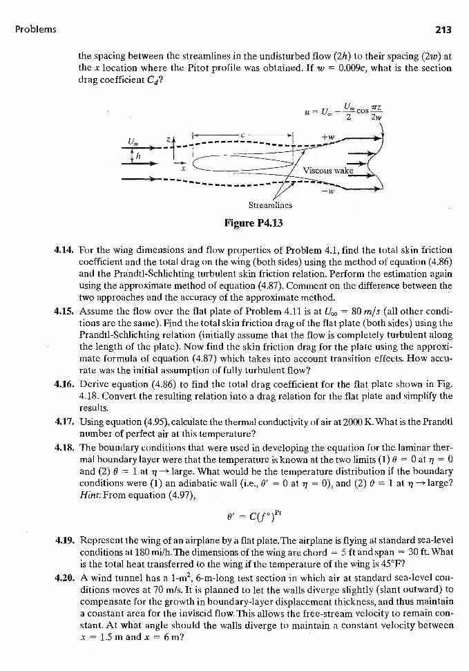
Problems 213
the spacing between the streamlines in the undisturbed flow (2h) to their spacing (2w) atthe x location where the Pitot profile was obtained. If w = O.009c, what is the sectiondrag coefficient Cd?
4.14. For the wing dimensions and flow properties of Problem 4.1, find the total skin frictioncoefficient and the total drag on the wing (both sides) using the method of equation (4.86)and the Prandtl-Schlichting turbulent skin friction relation. Perform the estimation againusing the approximate method of equation (4.87). Comment on the difference between thetwo approaches and the accuracy of the approximate method.
4.15. Assume the flow over the flat plate of Problem 4.11 is at = 80 rn/s (all other condi-tions are the same). Find the total skin friction drag of the flat plate (both sides) using thePrandtl-Schlichting relation (initially assume that the flow is completely turbulent alongthe length of the plate). Now find the skin friction drag for the plate using the approxi-mate formula of equation (4.87) which takes into account transition effects. How accu-rate was the initial assumption of fully turbulent flow?
4.16. Derive equation (4.86) to find the total drag coefficient for the flat plate shown in Fig.4.18. Convert the resulting relation into a drag relation for the flat plate and simplify theresults.
4.17. Using equation (4.95), calculate the thermal conductivity of air at 2000 K. What is the Prandtlnumber of perfect air at this temperature?
4.18. The boundary conditions that were used in developing the equation for the laminar ther-mal boundary layer were that the temperature is known at the two limits (1) 0 = 0 at = 0and (2) 0 = 1 at —+ large. What would be the temperature distribution if the boundaryconditions were (1) an adiabatic wall (i.e., 8' = 0 at rj = 0), and (2) 0 = 1 at ij large?Hint: From equation (4.97),
0' =
4.19. Represent the wing of an airplane by a flat plate. The airplane is flying at standard sea-levelconditions at 180 mi/h. The dimensions of the wing are chord = 5 ft and span = 30 ft. Whatis the total heat transferred to the wing if the temperature of the wing is 45°F?
4.20. A wind tunnel has a 1-rn2, 6-rn-long test section in which air at standard sea-level con-ditions moves at 70 rn/s. It is planned to let the walls diverge slightly (slant outward) tocompensate for the growth in boundary-layer displacement thickness, and thus maintaina constant area for the inviscid flow. This allows the free-stream velocity to remain con-stant. At what angle should the walls diverge to maintain a constant velocity betweenx = 1.5 m and x = 6 m?
U,,.,
I
x)r
Streamlines
Figure P4.13

Chap. 4 / Viscous Boundary Layers
REFERENCES
Abbott IH, von Doenhoff AE. 1949. Theory of Wing Sections. New York: Dover
CebeciT,Bradshaw P.1979. Momentum Transfer in Boundary Layers. NewYork: McGraw-Hill
CebeciT, Smith AMO. 1974.Analysis of Turbulent Boundary Layers. Orlando:Academic Press
DeJarnette FR, Ratciffe RA. 1996. Matching inviscid/boundary layer flowfields. AIAA .1.34:35—42
Dommasch DO, Sherby SS, Connolly TF. 1967. Airplane Aerodynamics. Ed. New York:Pitman
Dorrance WH. 1962. Viscous Hypersonic Flow. New York: McGraw-Hill
Head MR. 1969. work on entrainment. In Proceedings, Computation of TurbulentBoundary Layers—1968 AFOSR-IFP-Stanford Conference, Vol. 1. Stanford: StanfordUniversity Press
Neumann RD. 1989. Defining the aerothermodynamic environment. In Hypersonics, Vol I:Defining the Hypersonic Environment, Ed. Bertin 33, Glowinski R, Periaux 3. Boston:Birkhauser BostonSchlichting H. 1979. Boundary Layer Theory. 7th Ed. New York: McGraw-Hill
Smith BR. 1991. Application of turbulence modeling to the design of military aircraft.Presented at AIAA Aerosp. Sci. Meet., 29th, AIAA Pap. 91-0513, Reno, NV
Spalart PR, Alimaras SR.; 1992. A one-equation turbulence model for aerodynamic flows.Presented at AIAA Aerosp. Sci. Meet., 30th, AIAA Pap. 92-0439, Reno, NV
Spalart PR. 2000. Trends in turbulence treatments. Presented at Fluids 2000 Conf.,AIAA Pap.2000-2306, Denver, CO
White FM. 2005. Viscous Fluid Flow. Ed. New York: McGraw-Hill
Wilcox DC. 1998. Turbulence Modeling for CFD. Ed. LaCañada, CA: DCW Industries
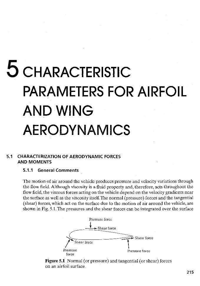
5 CHARACTERISTIC
PARAMETERS FOR AIRFOIL
AND WINGAERODYNAMICS
5.1 CHARACTERIZATION OF AERODYNAMIC FORCESAND MOMENTS
5.1.1 General Comments
The motion of air around the vehicle produces pressure and velocity variations throughthe flow field. Although viscosity is a fluid property and, therefore, acts throughout theflow field, the viscous forces acting on the vehicle depend on the velocity gradients nearthe surface as well as the viscosity itself. The normal (pressure) forces and the tangential(shear) forces, which act on the surface due to the motion of air around the vehicle, areshown in Fig. 5.1. The pressures and the shear forces can be integrated over the surface
Pressure force
Shear force
Shear forceShear force
Pressure Pressure forceforce
Figure 5.1 Normal (or pressure) and tangential (or shear) forceson an airfoil surface.
215
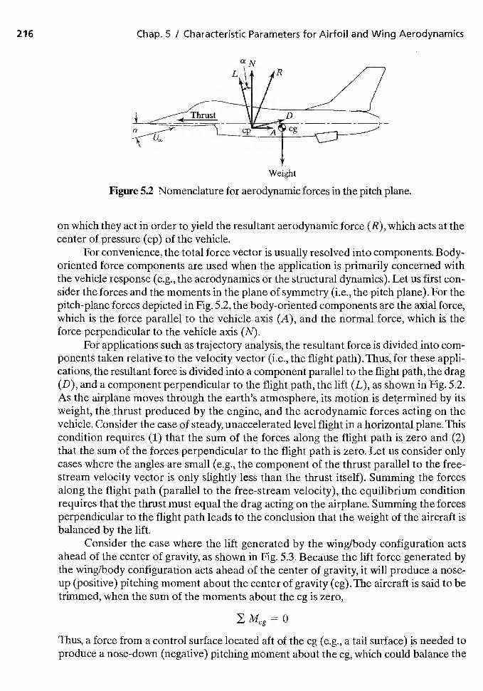
216 Chap. 5 / Characteristic Parameters for Airfoil and Wing Aerodynamics
Figure 5.2 Nomenclature for aerodynamic forces in the pitch plane.
on which they act in order to yield the resultant aerodynamic force (R), which acts at thecenter of pressure (cp) of the vehicle.
For convenience, the total force vector is usually resolved into components. Body-oriented force components are used when the application is primarily concerned withthe vehicle response (e.g., the aerodynamics or the structural dynamics). Let us first con-sider the forces and the moments in the plane of symmetry (i.e., the pitch plane). For thepitch-plane forces depicted in Fig. 5.2, the body-oriented components are the axial force,which is the force parallel to the vehicle axis (A), and the normal force, which is theforce perpendicular to the vehicle axis (N).
For applications such as trajectory analysis, the resultant force is divided into com-ponents taken relative to the velocity vector (i.e., the flight path).Thus, for these appli-cations, the resultant force is divided into a component parallel to the flight path, the drag(D), and a component perpendicular to the flight path, the lift (L), as shown in Fig. 5.2.As the airplane moves through the earth's atmosphere, its motion is determined by itsweight, the thrust produced by the engine, and the aerodynamic forces acting on thevehicle. Consider the case of steady, unaccelerated level flight in a horizontal plane. Thiscondition requires (1) that the sum of the forces along the flight path is zero and (2)that the sum of the forces perpendicular to the flight path is zero, Let us consider onlycases where the angles are small (e.g., the component of the thrust parallel to the free-stream velocity vector is only slightly less than the thrust itself). Summing the forcesalong the flight path (parallel to the free-stream velocity), the equilibrium conditionrequires that the thrust must equal the drag acting on the airplane. Summing the forcesperpendicular to the flight path leads to the conclusion that the weight of the aircraft isbalanced by the lift.
Consider the case where the lift generated by the wing/body configuration actsahead of the center of gravity, as shown in Fig. 5.3. Because the lift force generated bythe wing/body configuration acts ahead of the center of gravity, it will produce a nose-up (positive) pitching moment about the center of gravity (cg).The aircraft is said to betrimmed, when the sum of the moments about the cg is zero,
Thus, a force from a control surface located aft of the cg (e.g., a tail surface) is needed toproduce a nose-down (negative) pitching moment about the cg, which could balance the
Weight
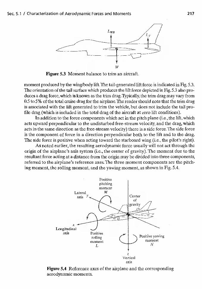
Sec. 5.1 / Characterization of Aerodynamic Forces and Moments 217
Figure 5.3 Moment balance to trim an aircraft.
moment produced by the wing/body lift.The tail-generated lift force is indicated in Fig. 5.3.The orientation of the tail surface which produces the lift force depicted in Fig. 5.3 also pro:duces a drag force, which is known as the trim drag. Typically, the trim drag may vary from0.5 to 5% ofthe total cruise drag for the airplane.The reader should note that the trim dragis associated with the lift generated to trim the vehicle, but does not include the tail pro-file drag (which is included in the total drag of the aircraft at zero lift conditions).
In addition to the force components which act in the pitch plane (i.e., the lift, whichacts upward perpendicular to the undisturbed free-stream velocity, and the drag, whichacts in the same direction as the free-stream velocity) there is a side force. The side forceis the component of force in a direction perpendicular both to the lift and to the drag.The side force is positive when acting toward the starboard wing (i.e., the pilot's right).
As noted earlier, the resulting aerodynamic force usually will not act through theorigin of the airplane's axis system (i.e., the center of gravity). The moment due to theresultant force acting at a distance from the origin may be divided into three components,referred to the airplane's reference axes. The three moment components are the pitch-ing moment, the rolling moment, and the yawing moment, as shown in Fig. 5.4.
xLongitudinal
axis
axis
Figure 5.4 Reference axes of the airplane and the correspondingaerodynamic moments.
w
Positivepitchingmoment
Lateral P4
axis Y. Center
Positiverolling
momentL
Positive yawingmoment
N
Vertical
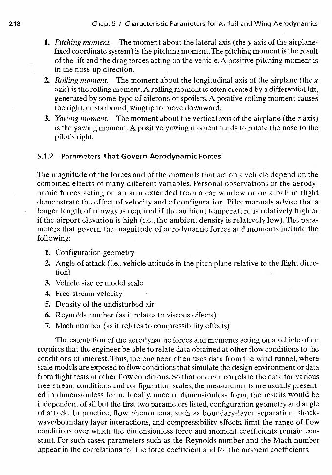
218 Chap. 5 I Characteristic Parameters for Airfoil and Wing Aerodynamics
1. Pitching moment. The moment about the lateral axis (the y axis of the airplane-fixed coordinate system) is the pitching moment. The pitching moment is the resultof the lift and the drag forces acting on the vehicle. A positive pitching moment isin the nose-up direction.
2. Rolling moment. The moment about the longitudinal axis of the airplane (the xaxis) is the rolling moment. A rolling moment is often created by a differential lift,generated by some type of ailerons or spoilers. A positive rolling moment causesthe right, or starboard, wingtip to move downward.
3. Yawing moment. The moment about the vertical axis of the airplane (the z axis)is the yawing moment. A positive yawing moment tends to rotate the nose to thepilot's right.
5.1.2 Parameters That Govern Aerodynamic Forces
The magnitude of the forces and of the moments that act on a vehicle depend on thecombined effects of many different variables. Personal observations of the aerody-namic forces acting on an arm extended from a car window or on a ball in flightdemonstrate the effect of velocity and of configuration. Pilot manuals advise that alonger length of runway is required if the ambient temperature is relatively high orif the airport elevation is high (i.e., the ambient density is relatively low). The para-meters that govern the magnitude of aerodynamic forces and moments include thefollowing:
1. Configuration geometry2. Angle of attack (i.e., vehicle attitude in the pitch plane relative to the flight direc-
tion)3. Vehicle size or model scale4. Free-stream velocity5. Density of the undisturbed air6. Reynolds number (as it relates to viscous effects)7. Mach number (as it relates to compressibility effects)
The calculation of the aerodynamic forces and moments acting on a vehicle oftenrequires that the engineer be able to relate data obtained at other flow conditions to theconditions of interest. Thus, the engineer often uses data from the wind tunnel, wherescale models are exposed to flow conditions that simulate the design environment or datafrom flight tests at other flow conditions. So that one can correlate the data for variousfree-stream conditions and configuration scales, the measurements are usually present-ed in dimensionless form. Ideally, once in dimensionless form, the results would beindependent of all but the first two parameters listed, configuration geometry and angleof attack. In practice, flow phenomena, such as boundary-layer separation, shock-wave/boundary-layer interactions, and compressibility effects, limit the range of flowconditions over which the dimensionless force and moment coefficients remain con-stant. For such cases, parameters such as the Reynolds number and the Mach numberappear in the correlations for the force coefficient and for the moment coefficients.
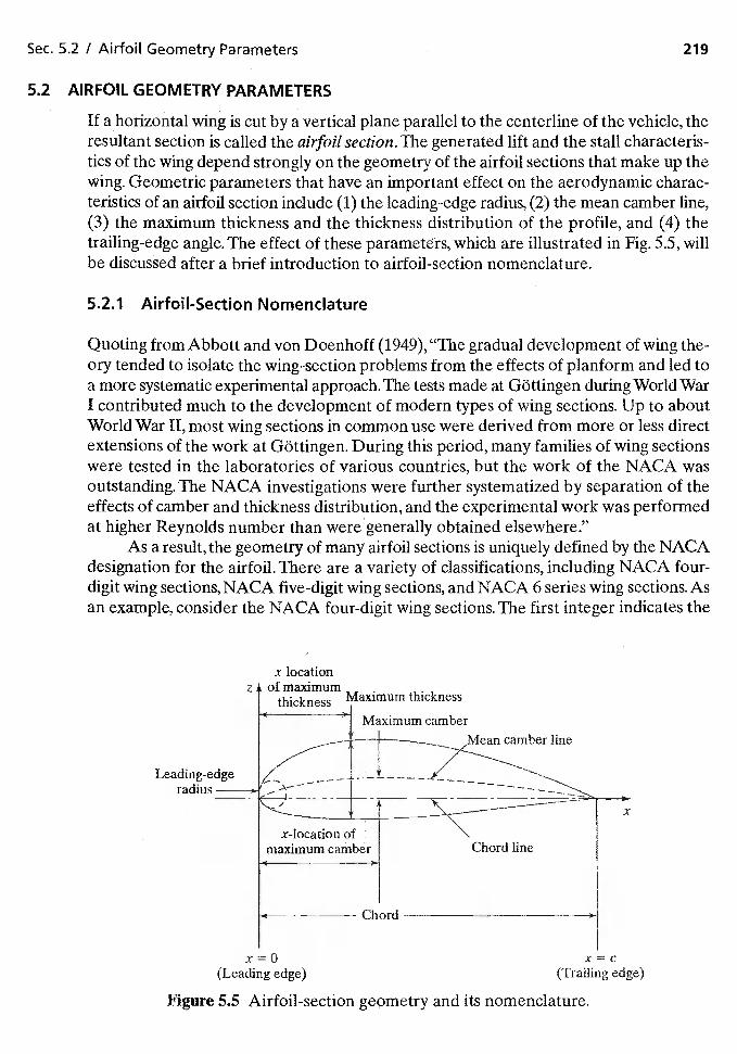
Sec. 5.2 / Airfoil Geometry Parameters 219
5.2 AIRFOIL GEOMETRY PARAMETERS
If a horizontal wing is cut by a vertical plane parallel to the centerline of the vehicle, theresultant section is called the airfoil section.The generated lift and the stall characteris-tics of the wing depend strongly on the geometry of the airfoil sections that make up thewing. Geometric parameters that have an important effect on the aerodynamic charac-teristics of an airfoil section include (1) the leading-edge radius, (2) the mean camber line,(3) the maximum thickness and the thickness distribution of the profile, and (4) thetrailing-edge angle. The effect of these parameters, which are illustrated in Fig. 5.5, willbe discussed after a brief introduction to airfoil-section nomenclature.
5.2.1 Airfoil-Section Nomenclature
Quoting from Abbott and von Doenhoff (1949), gradual development of wing the-ory tended to isolate the wing-section problems from the effects of planform and led toa more systematic experimental approach. The tests made at Gottingen during World WarI contributed much to the development of modern types of wing sections. Up to aboutWorld War II, most wing sections in common use were derived from more or less directextensions of the work at Gottingen. During this period, many families of wing sectionswere tested in the laboratories of various countries, but the work of the NACA wasoutstanding. The NACA investigations were further systematized by separation of theeffects of camber and thickness distribution, and the experimental work was performedat higher Reynolds number than were generally obtained elsewhere."
As a result, the geometry of many airfoil sections is uniquely defined by the NACAdesignation for the airfoil. There are a variety of classifications, including NACA four-digit wing sections, NACA five-digit wing sections, and NACA 6 series wing sections. Asan example, consider the NACA four-digit wing sections. The first integer indicates the
x=c(Trailing edge)
Figure 53 Airfoil-section geometry and its nomenclature.
x-locationz of maximum
thickness Maximum thickness
Maximum camber
x
Chord line
x0(Leading edge)
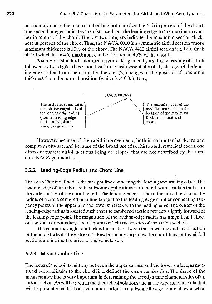
220 Chap. 5 / Characteristic Parameters for Airfoit and Wing Aerodynamics
maximum value of the mean camber-line ordinate (see Fig. 5.5) in percent of the chord.The second integer indicates the distance from the leading edge to the maximum cam-ber in tenths of the chord. The last two integers indicate the maximum section thick-ness in percent of the chord.Thus, the NACA 0010 is a symmetric airfoil section whosemaximum thickness is 10% of the chord. The NACA 4412 airfoil section is a 12% thickairfoil which has a 4% maximum camber located at 40% of the chord.
A series of "standard" modifications are designated by a suffix consisting of a dashfollowed by two digits. These modifications consist essentially of (1) changes of the lead-ing-edge radius from the normal value and (2) changes of the position of maximumthickness from the normal position (which is at 0.3c). Thus,
The first integer indicatesthe relative magnitude ofthe leading-edge radius(normal leading-edgeradius is "6"; sharpleading edge is "0").
NACA
The second integer of themodification indicates thelocation of the maximumthickness in tenths ofchord.
However, because of the rapid improvements, both in computer hardware andcomputer software, and because of the broad use of sophisticated numerical codes, oneoften encounters airfoil sections being developed that are not described by the Stan-dard NACA geometries.
5.2.2 Leading-Edge Radius and Chord Line
The chord line is defined as the straight line connecting the leading and trailing edges. Theleading edge of airfoils used in subsonic applications is rounded, with a radius that is onthe order of 1% of the chord length. The leading-edge radius of the airfoil section is theradius of a circle centered on a line tangent to the leading-edge camber connecting tan-gency points of the upper and the lower surfaces with the leading edge.The center of theleading-edge radius is located such that the cambered section projects slightly forward ofthe leading-edge point.The magnitude of the leading-edge radius has a significant effecton the stall (or boundary-layer separation) characteristics of the airfoil section.
The geometric angle of attack is the angle between the chord line and the directionof the undisturbed, "free-stream" flow. For many airplanes the chord lines of the airfoilsections are inclined relative to the vehicle axis.
5.2.3 Mean Camber Line
The locus of the points midway between the upper surface and the lower surface, as mea-sured perpendicular to the chord line, defines the mean camber line. The shape of themean camber line is very important in determining the aerodynamic characteristics of anairfoil section.As will be seen in the theoretical solutions and in the experimental data thatwill be presented in this book, cambered airfoils in a subsonic flow generate lift even when
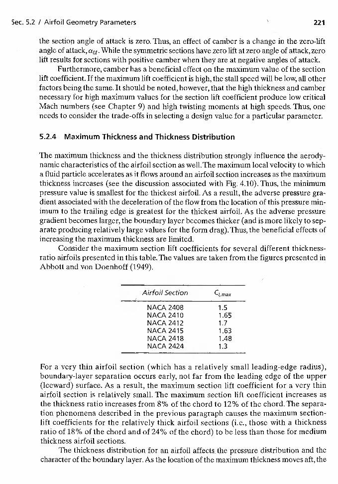
Sec. 5.2 / Airfoil Geometry Parameters 221
the section angle of attack is zero. Thus, an effect of camber is a change in the zero-liftangle of attack, aw. While the symmetric sections have zero lift at zero angle of attack, zerolift results for sections with positive camber when they are at negative angles of attack.
Furthermore, camber has a beneficial effect on the maximum value of the sectionlift coefficient. If the maximum lift coefficient is high, the stall speed will be low, all otherfactors being the same. It should be noted, however, that the high thickness and cambernecessary for high maximum values for the section lift coefficient produce low criticalMach numbers (see Chapter. 9) and high twisting moments at high speeds. Thus, oneneeds to consider the trade-offs in selecting a design value for a particular parameter.
5.2.4 Maximum Thickness and Thickness Distribution
The maximum thickness and the thickness distribution strongly influence the aerody-namic characteristics of the airfoil section as well. The maximum local velocity to whicha fluid particle accelerates as it flows around an airfoil section increases as the maximumthickness increases (see the discussion associated with Fig. 4.10). Thus, the minimumpressure value is smallest for the thickest airfoil. As a result, the adverse pressure gra-dient associated with the deceleration of the flow from the location of this pressure min-imum to the trailing edge is greatest for the thickest airfoil. As the adverse pressuregradient becomes larger, the boundary layer becomes thicker (and is more likely to sep-arate producing relatively large values for the form drag). Thus, the beneficial effects ofincreasing the maximum thickness are limited.
Consider the maximum section lift coefficients for several different thickness-ratio airfoils presented in this table. The values are taken from the figures presented inAbbott and von Doenhoff (1949).
Airfoil Section Cimax
NACA 2408 1.5NACA241O 1.65NACA 2412 1.7NACA 2415 1.63NACA 2418 1.48NACA 2424 1.3
For a very thin airfoil section (which has a relatively small leading-edge radius),boundary-layer separation occurs early, not far from the leading edge of the upper(leeward) surface. As a result, the maximum section lift coefficient for a very thinairfoil section is relatively small. The maximum section lift coefficient increases asthe thickness ratio increases from 8% of the chord to 12% of the chord. The separa-tion phenomena described in the previous paragraph causes the maximum section-lift coefficients for the relatively thick airfoil sections (i.e., those with a thicknessratio of 18% of the chord and of 24% of the chord) to be less than those for mediumthickness airfoil sections.
The thickness distribution for an airfoil affects, the pressure distribution and thecharacter of the boundary layer. As the location of the maximum thickness moves aft, the
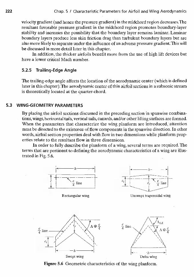
222 Chap. 5 / Characteristic Parameters for AfrfoU and Wing Aerodynamics
velocity gradient (and hence the pressure gradient) in the midchord region decreases. Theresultant favorable pressure gradient in the midchord region promotes boundary-layerstability and increases the possibility that the boundary layer remains laminar. Laminarboundary layers produce less skin friction drag than turbulent boundary layers but arealso more likely to separate under the influence of an adverse pressure gradient. This willbe discussed in more detail later in this chapter.
In addition, the thicker airfoils benefit more from the use of high lift devices buthave a lower critical Mach number.
5.2.5 Trailing-Edge Angle
The trailing-edge angle affects the location of the aerodynamic center (which is definedlater in this chapter).The aerodynamic center of thin airfoil sections in a subsonic streamis theoretically located at the quarter-chord.
5.3 WING-GEOMETRY PARAMETERS
By placing the airfoil sections discussed in the preceding section in spanwise combina-tions, wings, horizontal tails, vertical tails, canards, and/or other lifting surfaces are formed.When the parameters that characterize the wing planform are introduced; attentionmust be directed to the existence of flow components in the spanwise direction. In otherwords, airfoil section properties deal with flow in two dimensions while planform prop-erties relate to the resultant flow in three dimensions.
In order to fully describe the planform of a wing, several terms are required. Theterms that are pertinent to defining the aerodynamic characteristics of a wing are illus-trated in Fig. 5.6.
Li b
lane Cr line
Rectangular wing Unswept trapezoidal wing
line
Delta wing
Figure 5.6 Geometric characteristics of the wing planform.
Swept wing
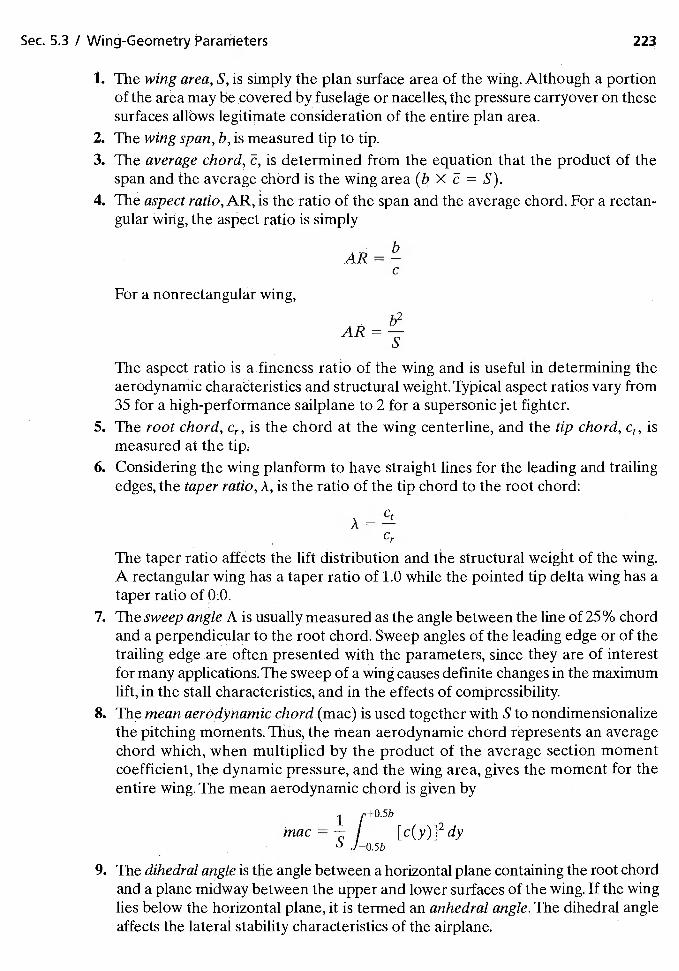
Sec. 5.3 I Wing-Geometry Parameters 223
1. The wing area, S, is simply the plan surface area of the wing. Although a portionof the area may be covered by fuselage or nacelles, the pressure carryover on thesesurfaces allows legitimate consideration of the entire plan area.
2. The wing span, b, is measured tip to tip.3. The average chord, is determined from the equation that the product of the
span and the average chord is the wing area (b X = S).4. The aspect ratio, AR, is the ratio of the span and the average chord. For a rectan-
gular wing, the aspect ratio is simply
C
For a nonrectangular wing,
b2
The aspect ratio is a fineness ratio of the wing and is useful in determining theaerodynamic characteristics and structural weight. Typical aspect ratios vary from35 for a high-performance sailplane to 2 for a supersonic jet fighter.
5. The root chord, is the chord at the wing centerline, and the tip chord, ismeasured at the tip.
6. Considering the wing planform to have straight lines for the leading and trailingedges, the taper ratio, A, is the ratio of the tip chord to the root chord:
Ct
Cr
The taper ratio affects the lift distribution and the structural weight of the wing.A rectangular wing has a taper ratio of 1.0 while the pointed tip delta wing has ataper ratio of 0.0.
7. The sweep angle A is usually measured as the angle between the line of 25% chordand a perpendicular to the root chord. Sweep angles of the leading edge or of thetrailing edge are often presented with the parameters, since they are of interestfor many applications. The sweep of a wing causes definite changes in the maximumlift, in the stall characteristics, and in the effects of compressibility.
8. The mean aerodynamic chord (mac) is used together with S to nondimensionalizethe pitching moments. Thus, the mean aerodynamic chord represents an averagechord which, when multiplied by the product of the average section momentcoefficient, the dynamic pressure, and the wing area, gives the moment for theentire wing. The mean aerodynamic chord is given by
1ç+O.5b
mac = — I [c(y)]2dyS J-O.5b
9. The dihedral angle is the angle between a horizontal plane containing the root chordand a plane midway between the upper and lower surfaces of the wing. If the winglies below the horizontal plane, it is termed an anhedral angle. The dihedral angleaffects the lateral stability characteristics of the airplane.
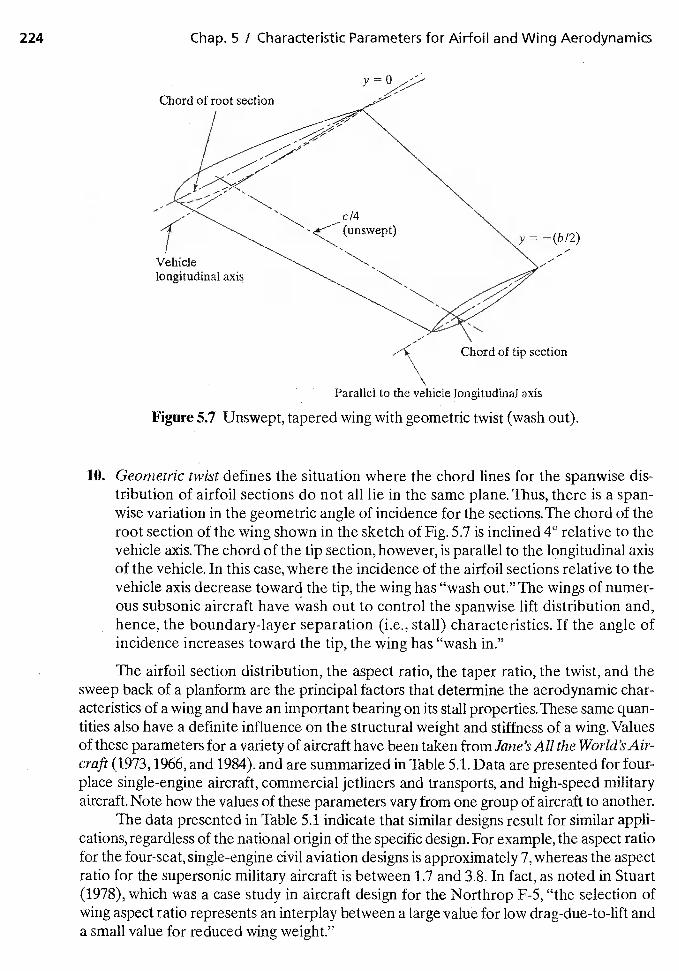
224 Chap. S / Characteristic Parameters for Airfoil and Wing Aerodynamics
Figure 5.7 Unswept, tapered wing with geometric twist (wash out).
10. Geometric twist defines the situation where the chord lines for the spanwise dis-tribution of airfoil sections do not all lie in the same plane. Thus, there is a span-wise variation in the geometric angle of incidence for the sections. The chord of theroot section of the wing shown in the sketch of Fig. 5.7 is inclined 4° relative to thevehicle axis. The chord of the tip section, however, is parallel to the longitudinal axisof the vehicle. In this case, where the incidence of the airfoil sections relative to thevehicle axis decrease toward the tip, the wing has "wash out." The wings of numer-ous subsonic aircraft have wash out to control the spanwise lift distribution and,hence, the boundary-layer separation (i.e., stall) characteristics. If the angle ofincidence increases toward the tip, the wing has "wash in."
The airfoil section distribution, the aspect ratio, the taper ratio, the twist, and thesweep back of a planform are the principal factors that determine the aerodynamic char-acteristics of a wing and have an important bearing on its stall properties. These same quan-tities also have a definite influence on the structural weight and stiffness of a wing. Valuesof these parameters for a variety of aircraft have been taken from Jane s All the World's Air-craft (1973,1966, and 1984). and are summarized in Table 5.1. Data are presented for four-place single-engine aircraft, commercial jetliners and transports, and high-speed militaryaircraft. Note how the values of these parameters vary from one group of aircraft to another.
The data presented in Table 5.1 indicate that similar designs result for similar appli-cations, regardless of the national origin of the specific design. For example, the aspect ratiofor the four-seat, single-engine civil aviation designs is approximately 7, whereas the aspectratio for the supersonic military aircraft is between 1.7 and 3.8. In fact, as noted in Stuart(1978), which was a case study in aircraft design for the Northrop F-5, "the selection ofwing aspect ratio represents an interplay between a large value for low drag-due-to-lift anda small value for reduced wing weight."
Chord of root section
Vehiclelongitudinal axis
Chord of tip section
Parallel to the vehicle longitudinal axis
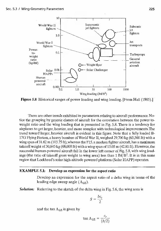
Sec. 53 / Wing-Geometry Parameters 225
Power-to-
weightratio
(hp/lbf)
Supersonicjet fighters
Wing loading (lbflft2)
Figure 5.8 Historical ranges of power loading and wing loading. [From Hall (1985).]
There are other trends exhibited in parameters relating to aircraft performance. No-tice the grouping by generic classes of aircraft for the correlation between the power-to-weight ratio and the wing loading that is presented in Fig. 5.8. There is a tendency forairplanes to get larger, heavier, and more complex with technological improvements. Thetrend toward larger, heavier aircraft is evident in this figure. Note that a fully loaded B-17G Flying Fortess, a heavy bomber of World War II, weighed 29,700 kg (65,500 lb) with awing span of 31.62 m (103.75 ft),'whereas the F15, a modem fighter aircraft, has a maximumtakeoff weight of 30,845 kg (68,000 ib) with a wing span of 13.05 m (42.81 ft). Howeyer, thesuccessful human-powered aircraft fall in the lower left corner of Fig. 5,8, with wing load-ings (the ratio of takeoff gross weight to wing area) less than 1 lbf/ft2. It is in this sameregion that Lockheed's solar high-altitude powered platform (Solar HAPP) operates.
EXAMPLE 5.1: Develop an expression for the aspect ratio
Develop an expression for the aspect ratio of a delta wing in terms of theleading edge sweep angle (ALE).
Solution: Referring to the sketch of the delta wing in Fig. 5.6, the wing area is
and the tan ALE is given by
bc
tan ALE= (b/2)
10
World War IIfighters
1.0
World War Ifighters
0.1
Wright flyer
Solar 0.01 Solar ChallengerHAPPs
Humanpowered
aircraft
Subsonic— jet
fighters
Jettransports
— Turboprops
Generalaviationaircraft
0.001 -0.1 1.0 10 100 1000
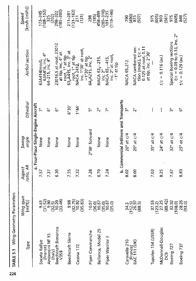
NT
AB
LE
5.1
Win
g-G
eom
etry
Par
amet
ers
Soc
ata
Ral
lye
(Fra
nce)
Am
bros
ini N
F 1
5(I
taly
)B
eech
craf
t Bon
anza
.V
35 B
Bee
chcr
aft S
ierr
a
Ces
sna
172
63A
41 4
(mod
),63
A41
6, in
c. 4
°64
—21
5, in
c. 4
°
2301
6.5
at r
oot,
2301
2at
tip,
inc.
4°
atro
ot, 1
°atti
p63
2A41
5, in
c. 3
0 at
root
, 1°a
t tip
NA
CA
241
2,in
c. 1
°30'
at r
oot,
—1°
30' a
t tip
642A
215,
inc.
20
NA
CA
inc.
2°
NA
CA
652
—41
5,in
c. 2
° at
roo
t,—
1°
at ti
p
173—
245
(108
—i 5
2)32
5(2
02)
2 98
—3
2 2
(185
—20
0)
21 1
—28
1(1
31—
162)
211
(131
)
298
(185
)45
8—49
9(2
85—
310)
191—
235
(119
—14
6)
Car
avel
le 2
10(F
ranc
e)B
AC
111
(U
K)
Tup
olev
154
(U
SS
R)
McD
onne
ll-D
ougl
asD
C9
Boe
ing
727
Boe
ing
737
34.3
(112
.5)
26.9
7(8
8.5)
37.5
5(1
23.2
)27
.25
(89.
42)
32.9
2(1
08.0
)28
.35
(93.
0)
b. C
omm
erci
al J
etlin
ers
and
Tra
nspo
rts
790
(490
)81
5(5
07)
975
(605
)90
3(5
61)
975
(605
)84
8(5
27)
Win
g sp
anA
spec
tS
wee
pS
peed
Typ
e[m
(ft)
]ra
tio, A
Ran
gle
Dih
edra
lA
irfoi
l sec
tion
[km
/h(m
i/h)]
9.61
(31.
52)
9.90
(32.
5)10
.20
(33.
46)
9.98
(32.
75)
10.9
2(3
5.83
)
10.9
7(3
6.0)
10.6
7(3
5.0)
10.6
7(3
5.0)
a. F
our-
Pla
ce S
ingl
e-E
ngin
e A
ircra
ft7.
57N
one
7°
7.37
Non
e6°
6.30
Non
e6°
7.35
Non
e6°
30'
7.32
Non
e1°
44'
2°30
' for
war
d5°
6.70
Non
e2°
7.24
Non
e70
Pip
er C
omm
anch
e
Bel
lanc
a, M
odel
25
Pip
er W
arrio
r II
8.02
20°
at ç
/43°
NA
CA
8.00
20°
at c
/42°
NA
CA
cam
bere
dtio
n (m
od.)
, t/c
=0.
125
at r
oot,
0.11
at ti
p, In
c. 2
°30'
7.03
35°
at c
/4
8.25
24°
at c
/4t/c
= 0
.116
(av
.)
7.67
32°
at c
/43°
Spe
cial
Boe
ing
sect
ions
tic =
0.0
9 to
0.1
3, in
c.2°
8.83
25°
at c
/46°
t/c =
0.1
29 (
av.)
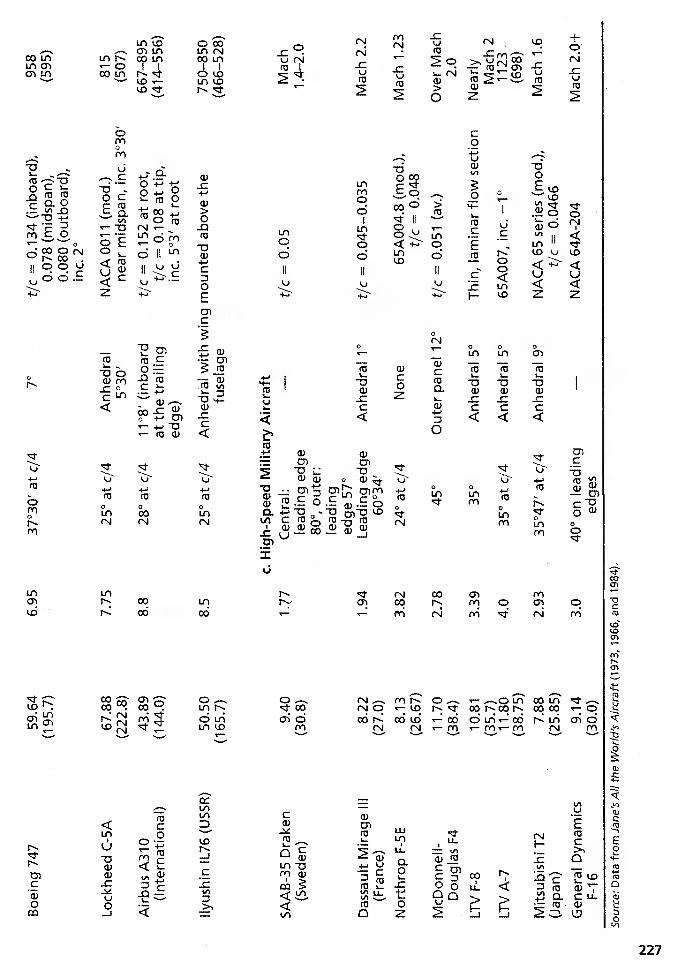
Boe
ing
747
59.6
46.
9537
°30'
at c
/47°
t/c =
0.1
34 (
inbo
ard)
,95
8(1
95.7
)0.
078
(mid
span
),(5
95)
0.08
0 (o
utbo
ard)
,in
c. 2
0
Lock
heed
C-5
A67
.88
7.75
25°
at c
/4A
nhed
ral
NA
CA
001
1 (m
od.)
815
(222
.8)
5°30
'ne
ar m
idsp
an, i
nc. 3
°30'
(507
)
Airb
us A
310
43.8
928
° at
c/4
1108
1 (in
boar
dt/c
= 0
.152
at r
oot,
667—
895
(Int
erna
tiona
l)(1
44.0
)at
the
trai
ling
t/c =
0.1
08 a
t tip
,(4
14—
556)
edge
)in
c. 5
°3' a
t roo
t
llyus
hin
1L76
(U
SS
R)
50.5
08.
525
° at
c/4
Anh
edra
l with
win
g m
ount
ed a
bove
the
750—
850
(165
,7)
fuse
lage
(466
—52
8)
c.H
igh-
Spee
d M
ilita
ry A
ircr
aft
SAA
B-3
5D
rake
n9.
401.
77C
entr
al:
t/c =
0.0
5M
ach
(Sw
eden
)(3
0.8)
lead
ing
edge
1.4—
2.0
80°,
out
er:
lead
ing
edge
57°
Das
saul
t Mira
ge II
I8.
221.
94Le
adin
g ed
geA
nhed
ral 1
°tIc
= 0
.045
—0.
035
Mac
h 2.
2(F
ranc
e)(2
7.0)
60°3
4'
Nor
thro
p F
-5E
8.13
3.82
24°
at c
/4N
one
65A
004.
8 (m
od.)
,M
ach
1.23
(26.
67)
tIc =
0.0
48
McD
onne
ll-11
.70
2.78
45°
Out
er p
anel
12°
t/c0.
051
(av.
)O
ver
Mac
hD
ougl
as F
4(3
8.4)
2.0
LTV
F-8
10.8
13.
3935
°A
nhed
ral5
°T
hin,
lam
inar
flow
sec
tion
Nea
rly(3
5.7)
Mac
h 2
LTV
A-7
11.8
04.
035
° at
c/4
Anh
edra
l5°
65A
007,
inc.
—1°
1123
(38.
75)
(698
)
Mits
ubis
hi 1
27.
882.
9335
°47'
at c
/4A
nhed
ral 9
°N
AC
A 6
5 se
ries
(mod
.),
Mac
h 1.
6(J
apan
)(2
5.85
)t/c
= 0
.046
6
Gen
eral
Dyn
amic
s9.
143.
040
° on
lead
ing
NA
CA
64A
-204
Mac
h 2.
0+F
-16
(30.
0)ed
ges
Sou
rce:
Dat
a fr
om J
ane'
s A
ll th
e W
orld
's A
ircra
ft (1
973,
196
6, a
nd 1
984)
.
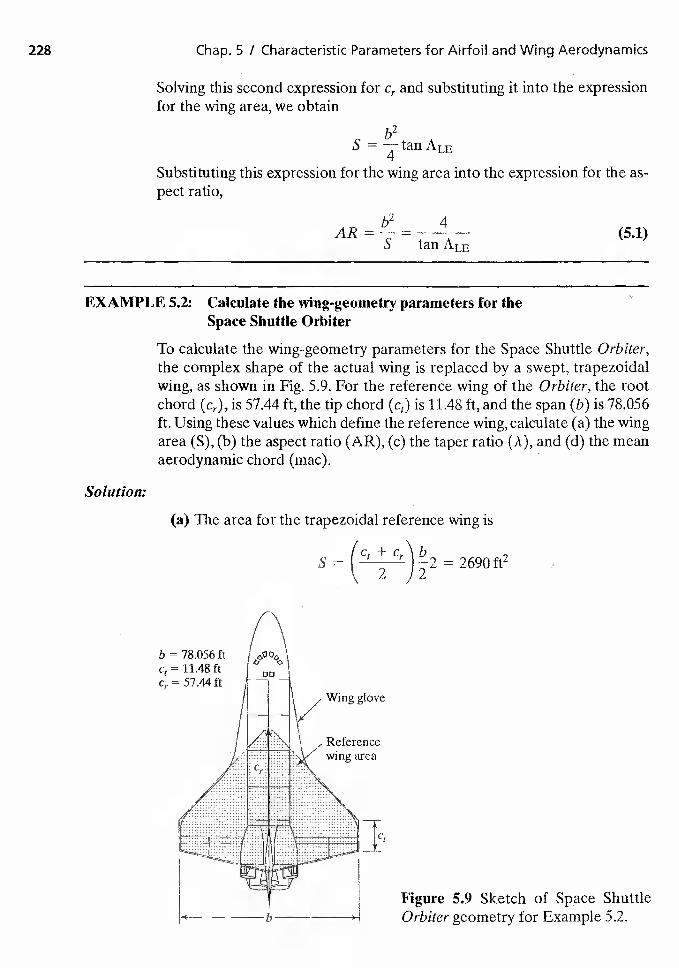
228 Chap. 5 / Characteristic Parameters for and Wing Aerodynamics
Solving this second expression for c,. and substituting it into the expressionfor the wing area, we obtain
b2S = —h-tan ALE
Substituting this expression for the wing area into the expression for the as-pect ratio,
AR— S — tanALE
EXAMPLE 5.2:
Solution:
Calculate the wing-geometry parameters for theSpace Shuttle Orbiter
To calculate the wing-geometry parameters for the Space Shuttle Orbiter,the complex shape of the actual wing is replaced by a swept, trapezoidalwing, as shown in Fig. 5.9. For the reference wing of the Orbiter, the rootchord (ci), is 57.44 It, the tip chord (ce) is 11.48 ft, and the span (b) is 78.056ft. Using these values which define the reference wing, calculate (a) the wingarea (5), (b) the aspect ratio (AR), (c) the taper ratio (A), and (d) the meanaerodynamic chord (mac).
(a) The area for the trapezoidal reference wing is
'Cf
Figure 5.9 Sketch of Space ShuttleOrbiter geometry for Example 5.2.
= cr)b= 2690ft2
b = 78.056 ft
57.44 ftWing glove
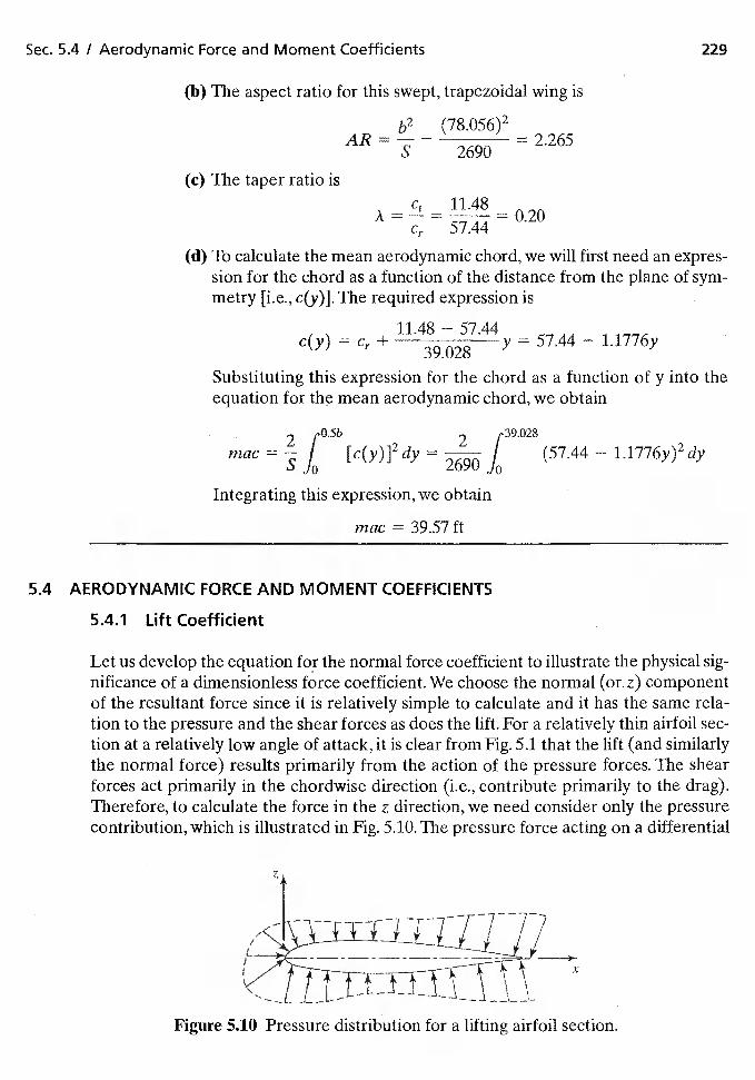
Sec. 5.4 / Aerodynamic Force and Moment Coefficients 229
(b)The aspect ratio for this swept, trapezoidal wing is
b2 (78.056)2AR
= = 2690= 2.265
(c) The taper ratio is11.48
=0.20Cr 57.44
(d) To calculate the mean aerodynamic chord, we will first need an expres-sion for the chord as a function of the distance from the plane of sym-metry [i.e., c(y)].The required expression is
11.48 — 57.44c(y) Cr
+ 39.02857.44 l.1776y
Substituting this expression for the chord as a function of y into theequation for the mean aerodynamic chord, we obtain
0.5b .39.028
mac f [c(y)]2dy2690!
(57.44 1.1776y)2dy
Integrating this expression, we obtain
mac = 39.57 ft
5.4 AERODYNAMIC FORCE AND MOMENT COEFFICIENTS
5.4.1 Lift Coefficient
Let us develop the equation for the normal force coefficient to illustrate the physical sig-nificance of a dimensionless force coefficient. We choose the normal z) componentof the resultant force since it is relatively simple to calculate and it has the same rela-tion to the pressure and the shear forces as does the lift. For a relatively thin airfoil sec-tion at a relatively low angle of attack, it is clear from Fig. 5.1 that the lift (and similarlythe normal force) results primarily from the action of the pressure forces. The shearforces act primarily in the chordwise direction (i.e., contribute primarily to the drag).Therefore, to calculate the force in the z direction, we need consider only the pressurecontribution, which is illustrated in Fig. 5.10. The pressure force acting on a differential
Figure 5.10 Pressure distribution for a lifting airfoil section.
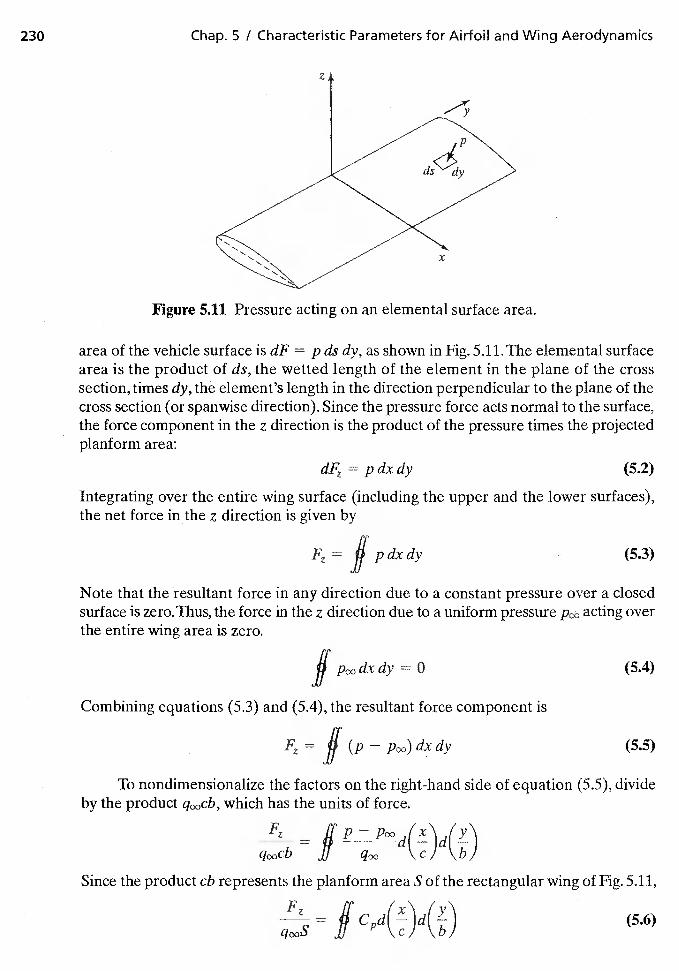
230 Chap. 5 / Characteristic Parameters for Airfoil and Wing Aerodynamics
Figure 5.11 Pressure acting on an elemental surface area.
area of the vehicle surface is dF = p ds dy, as shown in Fig. 5.1t The elemental surfacearea is the product of ds, the wetted length of the element in the plane of the crosssection, times dy, the element's length in the direction perpendicular to the plane of thecross section (or spanwise direction). Since the pressure force acts normal to the surface,the force component in the z direction is the product of the pressure times the projectedplanform area:
= p dx dy (5.2)
Integrating over the entire wing surface (including the upper and the lower surfaces),the net force in the z direction is given by
J pdxdy (5.3)
Note that the resultant force in any direction due to a constant pressure over a closedsurface is zero. Thus, the force in the z direction due to a uniform pressure acting overthe entire wing area is zero.
if (5.4)
Combining equations (5.3) and (5.4), the resultant force component is
= if (p - (5.5)
To nondimensionalize the factors on the right-hand side of equation (5.5), divideby the product which has the units of force.
=jj q00 \CJ \b
Since the product eb represents the planform area S of the rectangular wing of Fig. 5.11,
= if (5.6)
z
x
Sec. 5.4 / Aerodynamic Force and Moment Coefficients 231
When the boundary layer is thin, the pressure distribution around the airfoil is essentiallythat of an inviscid flow. Thus, the pressure distribution is independent of Reynoldsnumber and does not depend on whether the boundary layer is laminar or turbulent.When the boundary layer is thin, the pressure coefficient at.a particular location on thesurface given by the dimensionless coordinates (x/c, y/b) is independent of vehicle scaleand of the flow conditions. Over the range of flow conditions for which the pressurecoefficient is a unique function of the dimensionless coordinates (x/c, y/b), the value ofthe integral in equation (5.6) depends only on the configuration geometry and on theangle of attack. Thus, the resulting dimensionless force parameter, or force coefficient(in this case, the normal force coefficient), is independent of model scale and of flowconditions.
A similar analysis can be used to calculate the lift coefficient, which is defined as
CL = —f-— (5.7)
Data are presented in Fig. 5.12 for a NACA 23012 airfoil; that is, the wind-tunnelmodel represented a wing of infinite span. The lift acting on a wing of infinite span doesnot vary in the y direction. For this two-dimensional flow, we are interested in deter-mining the lift acting on a unit width of the wing [i.e., the lift per unit span (1)]. Thus, thelift measurements are presented in terms of the section lift coefficient C1. The sectionlift coefficient is the lift per unit span (1) divided by the product of the dynamic pressuretimes the plan area per unit span, which is the chord length (c).
C1 = —f--- (5.8)
The data from Abbott and von Doenhoff (1949) were obtained in a wind tunnel thatcould be operated at pressures up to 10 atm. As a result, the Reynolds number rangedfrom 3 X 10⁶ to 9 x 10⁶ at Mach numbers less than 0.17. In addition to the measure-ments obtained with a smooth model, data are presented for a model that had "standard"surface roughness applied near the leading edge. Additional comments will be madeabout surface roughness later in this chapter.
The experimental section lift coefficient is independent of Reynolds number andis a linear function of the angle of attack from —10° to + 10°. The slope of this linear por-tion of the curve is called the two-dimensional lift-curve slope. Using the experimentaldata for this airfoil,
dC1= = 0.104 per degree
Note that equations to be developed in Chapter 6 will show that the theoretical valuefor the two-dimensional lift-curve slope is per radian (0.1097 per degree).
Since the NACA 23012 airfoil section is cambered (the maximum camber is approx-imately 2% of the chord length), lift is generated at zero angle of attack. In fact, zero liftis obtained at —1.2°, which is designated or the section angle of attack for zero lift.As the angle of attack is increased above 10°, the section lift coefficient continues toincrease (but not linearly with angle of attack) until a maximum value, C1, max, is reached.Referring to Fig. 5.12, C1 max is 1.79 and occurs at an angle of attack of 18°. Partly because
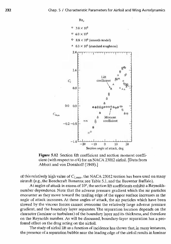
232 Chap. 5 / Characteristic Parameters for Airfoil and Wing Aerodynamics
o 3.0X10⁶
6.0x10⁶
8.8 X 10⁶ (smooth model)
6.0 X 10⁶ (standard roughness)
2.1
1.6
Lift -
C, coefficient o
0.8 \;
0.0 0.0 - -
C /Moment
o ci coefficient—0.2 —0.8 -
*DO
—1.6 liii I
—20 —10 0 10 20Section angle of attack, deg
Figure 5.12 Section lift coefficient and section moment coeffi-cient (with respect to c14) for an NACA 23012 airfoil. [Data fromAbbott and von Doenhoff (1949).]
of this relatively high value of C1 max' the NACA 23012 section has been used on manyaircraft (e.g., the Beechcraft Bonanza; see Table 5.1, and the Brewster Buffalo).
At angles of attack in excess of 10°, the section lift coefficients exhibit a Reynolds-number dependence. Note that the adverse pressure gradient which the air particlesencounter as they move toward the trailing edge of the upper surface increases as theangle of attack increases. At these angles of attack, the air particles which have beenslowed by the viscous forces cannot overcome the relatively large adverse pressuregradient, and the boundary layer separates. The separation location depends on thecharacter (laminar or turbulent) of the boundary layer and its thickness, and thereforeon the Reynolds number. As will be discussed, boundary-layer separation has a pro-found effect on the drag acting on the airfoil.
The study of airfoil lift as a function of incidence has shown that, in many instances,the presence of a separation bubble near the leading edge of the airfoil results in laminar
Sec. 5.4 / Aerodynamic Force and Moment Coefficients 233
section stall. Experimental data on two-dimensional "peaky" airfoil sections indicatethat as limited by laminar stall, is strongly dependent on the leading-edge shapeand on the Reynolds number. If the laminar boundary layer, which develops near theleading edge of the upper surface of the airfoil, is subjected to a relatively high adversepressure gradient, it will separate because the relatively low kinetic energy level of theair particles 'near the wall is insufficient to surmount the "pressure hill" of the adversepressure gradient. The separated shear layer that is formed may curve back onto thesurface within a very short distance. This is known as short bubble separation. Theseparated viscous layer near the pressure peak may not reattach to the surface at all, orit may reattach within 0.3 chord length or more downstream. This extended separationregion is known as long bubble separation.
The separation bubble may not appear at all on relatively thick, strongly camberedprofiles operating at high Reynolds numbers. The reason for this is that the Reynoldsnumber is then large enough for a natural transition to a turbulent boundary layer tooccur upstream of the strong pressure rise. The relatively high kinetic energy of the airparticles in a turbulent boundary layer permits them to climb the "pressure hill," andboundary-layer separation occurs only a short distance upstream of the trailing edge(trailing-edge stall).The separation point moves upstream continuously with increasingangle of attack, and the lift does not drop abruptly after Cimax but decreases gradually.
EXAMPLE 5.3: Calculate the lift per unit span on a NACA 23012 airfoilsection
Consider tests of an unswept wing that spans the wind tunnel and whoseairfoil section is NACA 23012. Since the wing model spans the test section,we will assume that the flow is two dimensional. The chord of the model is1.3 m. The test section conditions simulate a density altitude of 3 km. Thevelocity in the test section is 360 km/h.
What is the li.ft per unit span (in N/rn) that you would expect to measurewhen the angle of attack is 4°? What would be the corresponding section liftcoefficient?
Solution: First, we need to calculate the section lift coefficient. We will assume that thelift is a linear function of the angle of attack and that it is independent of theReynolds number (i.e., the viscous effects are negligible) at these test con-ditions. That these are reasonable assumptions can be seen by referring toFig. 5.12. Thus, the section lift coefficient is
C1 = Gia(a aol) (5.9)
Using the values presented in the discussion associated with Fig. 5.12,
C1 = 0.104(4.0 — (—1.2)) = 0.541
At an angle of attack of 4°, the experimental values of the section lift coef-ficient for an NACA 23012 airfoil section range from 0.50 to 0.57.
To calculate the conesponding lift force per unit span, we rearrangeequation (5.8) to obtain
/ =
234 Chap. 5 / Characteristic Parameters for Airfoil and Wing Aerodynamics
To calculate the dynamic pressure we need the velocity in rn/s andthe density in kg/m3.
kml000m h m360 100
h km 3600s S
Given the density altitude is 3 km, we refer to Table 1.2 to find that
= 0.74225PSL
(Note: The fact that we are given the density altitude as 3 km does notprovide specific information either about the temperature or about thepressure.)
p = =m m
Thus, the lift per unit span is
1 = ](1.3 m)
1 = (0.541)[4546.5-](1.3m) =
5.4.2 Moment Coefficient
The moment created by the aerodynamic forces acting on a wing (or airfoil) is deter-mined about a particular reference axis. The reference axis may be the leading edge,the quarter-chord location, the aerodynamic center, and so on. The significance ofthese reference axes in relation to the coefficients for thin airfoils will be discussed insubsequent chapters.
The procedure used to nondimensionalize the moments created by the aerody-namic forces is similar to that used to nondimensionalize the lift. To demonstrate thisnondimensionalization, the pitching moment about the leading edge due to the pres-sures acting on the surface will be calculated (refer again to Fig. 5.11).The contributionof the chordwise component of the pressure force and of the skin friction force to thepitching moment is small and is neglected.Thus, the pitching moment about the leadingedge due to the pressure force acting on the surface element whose area is ds times dyand which is located at a distance x from the leading edge is
dM0 = p dx dy x (5.10)
where dx dy is the projected area. Integrating over the entire wing surface, the net pitch-ing moment is given by
M0= J px dx dy (5.11)
When a uniform pressure acts on any closed surface, the resultant pitching moment dueto this constant pressure is zero. Thus,
Sec. 5.4 / Aerodynamic Force and Moment Coefficients 235
if (5.12)
Combiningequations (5.11) and (5.12), the resulting pitching moment about the leadingedge is
M0 if (p — (5.13)
To nondimensionalize the factors on the right-hand side of equation (5.13), divideby which has the units of force times length:
M0—
q00c2b — if c '\b
Since the product of cb represents the planform area of the wing 5,
If x/x\/y'\= if (5.14)
Thus, the dimensionless moment coefficient is
CM0M0
(5.15)
Since the derivation of equation (5.15) was for the rectangular wing of Fig. 5.11, the chordc is used. However, as noted previously in this chapter, the mean aerodynamic chord isused together with S to nondimensionalize the pitching moment for a general wing.
The section moment coefficient is used to represent the dimensionless momentper unit span (mo):
m0Cm0 (5.16)
since the surface area per unit span is the chord length c. The section pitching momentcoefficient depends on the camber and on the thickness ratio. Section pitching momentcoefficients for a NACA 23012 airfoil section with respect to the quarter chord and withrespect to the aerodynamic center are presented in Figs. 5.12 and 5.13, respectively. Theaerodynamic center is that point about which the section moment coefficient is inde-pendent of the angle of attack. Thus, the aerodynamic center is that point along thechord where all changes in lift effectively take place. Since the moment about the aero-dynamic center is the product of a force (the lift that acts at the center of pressure) anda lever arm (the distance from the aerodynamic center to the center of pressure), thecenter of pressure must move toward the aerodynamic center as the lift increases. Thequarter-chord location is significant, since it is the theoretical aerodynamic center forincompressible flow about a two-dimensional airfoil.
Note that the pitching moment coefficient is independent of the Reynolds number(for those angles of attack where the lift coefficient is independent of the Reynoldsnumber), since the pressure coefficient depends only on the dimensionless space coor-dinates (x/c, y/b) {see equation (5.14)}. One of the features of the NACA 23012 sectionis a relatively high Cj,max with only a small
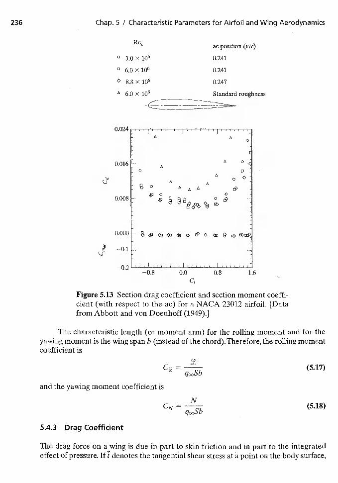
236 Chap. 5 / Characteristic Parameters for Airfoil and Wing Aerodynamics
ac position (xlc)
o 3.0 x 10⁶ 0.241
6.0 x 10⁶ 0.241
<> 8.8 X 10⁶ 0.247
A 6.0 x 10⁶ Standard roughness
III,A
0.016- A
0 UA
0A0 A A A
00.008-
—0.1 - -
—0.2 11111 I II 1111110.0 0.8 1.6
Cl
Figure 5.13 Section drag coefficient and section moment coeffi-cient (with respect to the ac) for a NACA 23012 airfoil. [Datafrom Abbott and von Doenhoff (1949).]
The characteristic length (or moment arm) for the rolling moment and for theyawing moment is the wing span b (instead of the chord).Therefore, the rolling momentcoefficient is
= (5.17)
and the yawing moment coefficient is
NCN = (5.18)
5.4.3 Drag Coefficient
The drag force on a wing is due in part to skin friction and in part to the integratedeffect of pressure. If t denotes the tangential shear stress at a point on the body surface,
Sec. 5.4 / Aerodynamic Force and Moment Coefficients 237
p the static pressure, and the external normal to the element of surface dS, the dragcan be formally expressed as
D = if (5.19)
where is a unit vector parallel to the free stream and the integration takes place overthe entire wetted surface. The first integral represents the friction component and thesecond integral represents the pressure drag.
The most straightforward approach to calculating the pressure drag is to perform thenumerical integration indicated by the second term in equation (5.19). This approach isknown as the near-field method of drag computation. Unfortunately, this can be a relativelyinaccurate procedure for streamlined configurations at small angles of attack. The inac-curacy results because the pressure drag integral is the difference between the integra-tion on forward-facing and rearward-facing surface elements, this difference being asecond-order quantity for slender bodies. Furthermore, the reader should realize that sub-tle differences between the computed pressure distribution and the actual pressure distri-bution can have a significant effect on the validity of the drag estimates, depending uponwhere the differences occur. If the pressure difference is near the middle of the aerodynamicconfiguration, where the local slope is roughly parallel to the free-stream direction, it willhave a relatively small effect on the validity of the estimated drag. However, if the pressuredifference is near the aft end of the configuration (for instance, on a nozzle boattail), evena small difference between the computed pressure and the actual pressure can have asignificant effect on the accuracy of the predicted drag.
In Chapter 3 we learned that zero drag results for irrotational, steady, incom-pressible flow past a two-dimensional body. For an airfoil section (i.e., a two-dimensionalgeometry) which is at a relatively low angle of attack so that the boundary layer is thinand does not separate, the pressure distribution is essentially that for an inviscid flow.Thus, skin friction is a major component of the chordwise force per unit span (fr).Referring to Figs. 5.1 and 5.10, can be approximated as
rdx (5.20)
where is the chordwise force per unit span due to skin friction. Dividing both sidesof equation (5.20) by the product yields an expression for the dimensionless forcecoefficient:
sf ICfd( —) (5.21)
j \cJCf, the skin friction coefficient, is defined as
Cf=12
(5.22)
As was stated in the general discussion of the boundaiy-layer characteristics in Chapter 4(see Fig. 4.18), skin friction for a turbulent boundary layer is much greater than thatfor a laminar boundary layer for given flow conditions. Equations for calculating the
238 Chap. 5 / Characteristic Parameters for Airfoil and Wing Aerodynamics
skin friction coefficient were developed in Chapter 4. However, let us introduce the cor-relations for the skin friction coefficient for incompressible flow past a flat plate to gaininsight into the force coefficient of equation (5.21). Of course, the results for a flat plateonly approximate those for an airfoil. The potential function given by equation (3.35a)shows that the velocity at the edge of the boundary layer and, therefore, the local stat-ic pressure, is constant along the plate. Such is not the case for an airfoil section, forwhich the flow accelerates from a forward stagnation point to a maximum velocity, thendecelerates to the trailing edge. Nevertheless, the analysis will provide useful insights intothe section drag coefficient,
Cd = (5.23)
for an airfoil at relatively low angles of attack.Referring to Chapter 4, when the boundary layer is laminar,
= 0.664(5.24)
(Re1)°'5
If the boundary layer is turbulent,
= 0.0583(5.25)
For equations (5.24) and (5.25), the local Reynolds number is defined as
Re1 (5.26)JLoo
Also, as was shown in Chapter 4, total skin-friction coefficients can be deflned.The totalskin-friction coefficient for laminar flow is given by
— 1.328Cf = (5.27)
and the total skin-friction coefficient for turbulent flow is
= 0.074(5.28)
which is the Prandtl formulation; although the Prandtl-Schlichting formulation is moreaccurate:
C0.455
258 (5.29)
These total skin-friction coefficients use the length-based Reynolds number given by
Rer= pcxUooL
(5.30)
where L is the length of a flat plate.
Sec. 5.4 / Aerodynamic Force and Moment Coefficients 239
EXAMPLE 54: Calculate the local skin friction
Calculate the local skin friction at a point 0.5 m from the leading edge of aflat-plate airfoil flying at 60 mIs at a height of 6 km.
Solution: Refer to Table 1.2 to obtain the static properties of undisturbed air at 6 km:
= 0.6601 kg/rn3
= 1.5949 X 10⁵kg/s'm
Thus, using equation (5.26),
(0.6601 kg/m3)(60 m/s)(0.5 m)
1.5949 x 10 5kg/s'm
= 1.242 X 10⁶
If the boundary layer is laminar,
Cf= 0.664
= 5.959 X
i—. (1 TT2 \ — 2T —
If the boundary layer is turbulent,
Cf = 0.0583= 3.522 x
(Ret )02
T = = 4.185 N/rn2
As discussed in the text of Chapter 2 and in the homework problems of Chapters2 and 4, the integral form of the momentum equation can be used to determine the dragacting on an airfoil section. This approach is known as the far-field method of dragdetermination. Wing-section profile-drag measurements have been made for the Boe-ing 727 in flight using the Boeing Airborne Traversing Probe, examples of which arepresented in Fig. 5. The probe consists of four main components: (1) flow sensors, (2)a rotating arm, (3) the drive unit, and (4) the mounting base. As reported by Bowes(1974), "The measured minimum section profile drag at M = .73 was about 15 percenthigher than predicted from wind-tunnel test data for a smooth airfoil. The wind-tunneldata used in this correlation were also from wake surveys on the 727 wing. The datawere adjusted to fully turbulent flow and extrapolated to flight Reynolds numbers. Thisquite sizeable difference between the measured and extrapolated values of Cd,mjn hasbeen attributed to surface roughness and excrescences on the airplane wing, althoughthe 15-percent increase in wing-section profile drag is larger than traditionally allottedin airplane drag estimates. The wing section where this survey was performed wasinspected and had numerous steps and bumps due to control devices and manufactur-ing tolerances which would account for this local level of excrescence drag. This is notrepresentative of the entire wing surface."
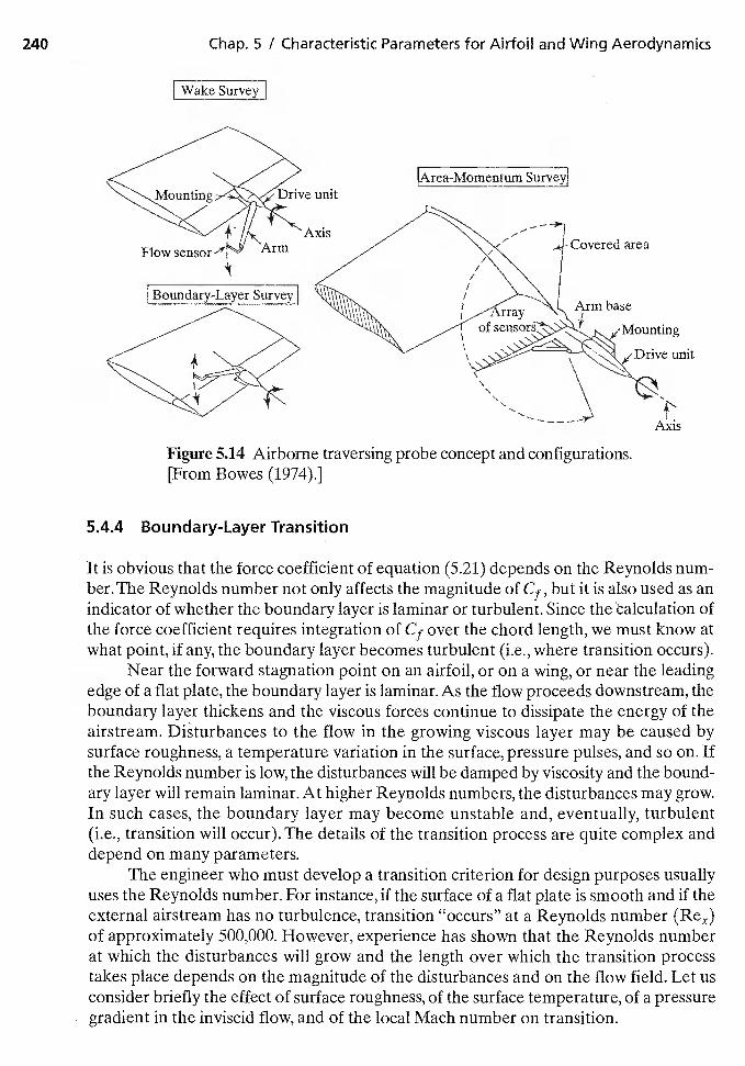
240 Chap. 5 / Characteristic Parameters for Airfoi' and Wing Aerodynamics
Wake Survey
lArea-Momentum Surveyj
Figure 5.14 Airborne traversing probe concept and configurations.[From B owes (1974).]
5.4.4 Boundary-Layer Transition
it is obvious that the force coefficient of equation (5.21) depends on the Reynolds num-ber. The Reynolds number not oniy affects the magnitude of Cf, but it is also used as anindicator of whether the boundary layer is laminar or turbulent. Since the calculation ofthe force coefficient requires integration of Cf over the chord length, we must know atwhat point, if any, the boundary layer becomes turbulent (i.e., where transition occurs).
Near the forward stagnation point on an airfoil, or on a wing, or near the leadingedge of a flat plate, the boundary layer is laminar. As the flow proceeds downstream, theboundary layer thickens and the viscous forces continue to dissipate the energy of theairstream. Disturbances to the flow in the growing viscous layer may be caused bysurface roughness, a temperature variation in the surface, pressure pulses, and so on. ifthe Reynolds number is low, the disturbances will be damped by viscosity and the bound-ary layer will remain laminar. At higher Reynolds numbers, the disturbances may grow.in such cases, the boundary layer may become unstable and, eventually, turbulent(i.e., transition will occur). The details of the transition process are quite complex anddepend on many parameters.
The engineer who must develop a transition criterion for design purposes usuallyuses the Reynolds number. For instance, if the surface of a flat plate is smooth and if theexternal airstream has no turbulence, transition "occurs" at a Reynolds number (Rex)of approximately 500,000, However, experience has shown that the Reynolds numberat which the disturbances will grow and the length over which the transition processtakes place depends on the magnitude of the disturbances and on the flow field. Let usconsider briefly the effect of surface roughness, of the surface temperature, of a pressuregradient in the inviscid flow, and of the local Mach number on transition.
Mounting Drive unit
4: AxisFlow sensor Arm area
Arm base
'Drive unit
\
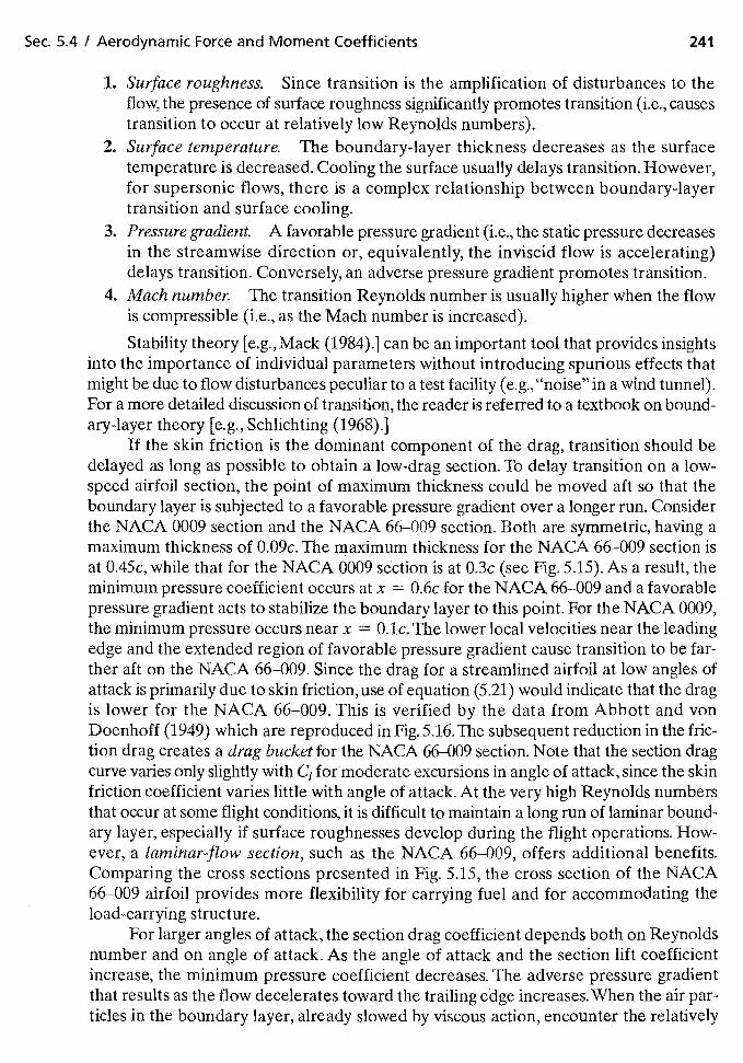
Sec. 5.4 / Aerodynamic Force and Moment Coefficients 241
1. Surface roughness. Since transition is the amplification of disturbances to theflow, the presence of surface roughness significantly promotes transition (i.e., causestransition to occur at relatively low Reynolds numbers).
2. Surface temperature. The boundary-layer thickness decreases as the surfacetemperature is decreased. Cooling the surface usually delays transition. However,for supersonic flows, there is a complex relationship between boundary-layertransition and surface cooling.
3. Pressure gradient. A favorable pressure gradient (i.e., the static pressure decreasesin the streamwise direction or, equivalently, the inviscid flow is accelerating)delays transition. Conversely, an adverse pressure gradient promotes transition.
4. Mach number. The transition Reynolds number is usually higher when the flowis compressible (i.e., as the Mach number is increased).
Stability theory [e.g., Mack (1984).] can be an important tool that provides insightsinto the importance of individual parameters without introducing spurious effects thatmight be due to flow disturbances peculiar to a test facility (e.g., "noise" in a wind tunnel).For a more detailed discussion of transition, the reader is referred to a textbook on bound-ary-layer theory [e.g., Schlichting (1968).]
If the skin friction is the dominant component of the drag, transition should bedelayed as long as possible to obtain a low-drag section, To delay transition on a low-speed airfoil section, the point of maximum thickness could be moved aft so that theboundary layer is subjected to a favorable pressure gradient over a longer run. Considerthe NACA 0009 section and the NACA 66—009 section. Both are symmetric, having amaximum thickness of 0.09c. The maximum thickness for the NACA 66—009 section isat 0.45c, while that for the NACA 0009 section is at 0.3c (see Fig. 5.15). As a result, theminimum pressure coefficient occurs at x = 0.6c for the NACA 66—009 and a favorablepressure gradient acts to stabilize the boundary layer to this point. For the NACA 0009,the minimum pressure occurs near x = 0.lc.The lower local velocities near the leadingedge and the extended region of favorable pressure gradient cause transition to be far-ther aft on the NACA 66—009. Since the drag for a streamlined airfoil at low angles ofattack is primarily due to skin friction, use of equation (5.21) would indicate that the dragis lower for the NACA 66—009. This is verified by the data from Abbott and vonDoenhoff (1949) which are reproduced in Fig. 5.16.The subsequent reduction in the fric-tion drag creates a drag bucket for the NACA 66—009 section. Note that the section dragcurve varies only slightly with C1 for moderate excursions in angle of attack, since the skinfriction coefficient varies little with angle of attack. At the very high Reynolds numbersthat occur at some flight conditions, it is difficult to maintain a long run of laminar bound-ary layer, especially if surface roughnesses develop during the flight operations. How-ever, a laminar-flow section, such as the NACA 66—009, offers additional benefits.Comparing the cross sections presented in Fig. 5.15, the cross section of the NACA66—009 airfoil provides more flexibility for carrying fuel and for accommodating theload-carrying structure.
For larger angles of attack, the section drag coefficient depends both on Reynoldsnumber and on angle of attack. As the angle of attack and the section lift coefficientincrease, the minimum pressure coefficient decreases. The adverse pressure gradientthat results as the flow decelerates toward the trailing edge increases, When the air par-ticles in the boundary layer, already slowed by viscous action, encounter the relatively
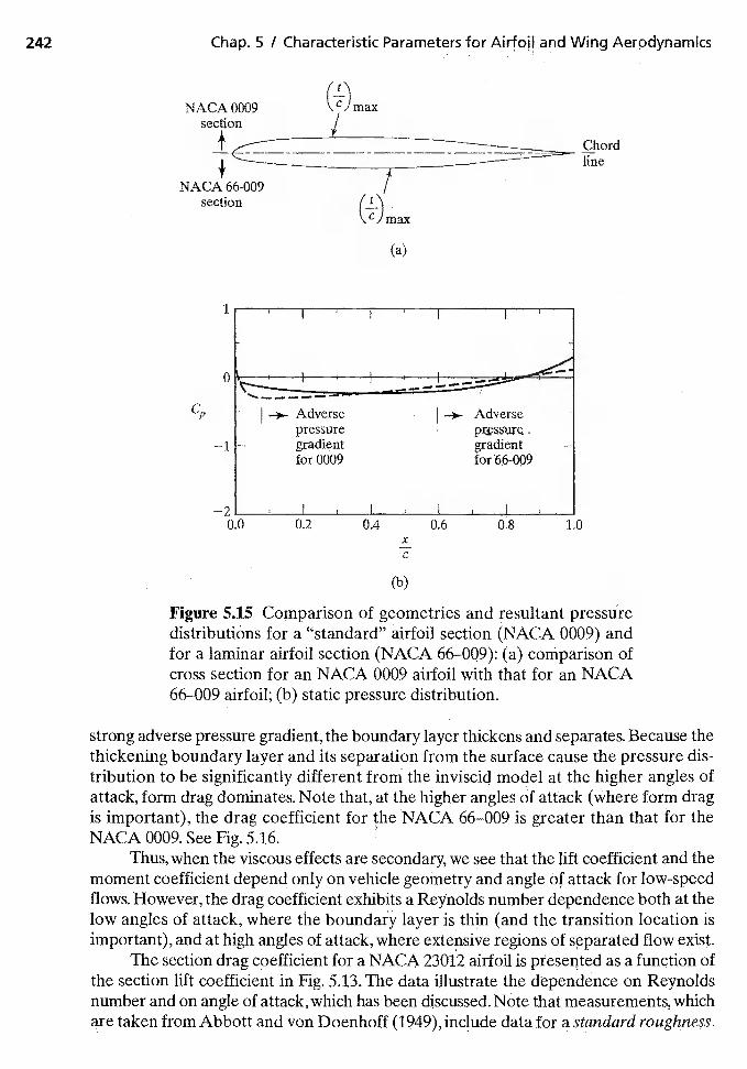
242 Chap. 5 / Characteristic Parameters for Airfol! and Wing Aerodynamics
NACA
section
(a)
11I
o
Cp—*.- Adverse Adverse
pressure—i gradient gradient
for 0009 for 66-009
—2 I I
0.0 0.2 0.4 0.6 0.8 1.0xC
(b)
Figure 5.15 Comparison of geometries and resultant pressuredistributions for a "standard" airfoil section (NACA 0009) andfor a laminar airfoil section (NACA 66—009): (a) comparison ofcross section for an NACA 0009 airfoil with that for an NACA66—009 airfoil; (b) static pressure distribution.
strong adverse pressure gradient, the boundary layer thickens and separates. Because thethickening boundary layer and its separation from the surface cause the pressure dis-tribution to be significantly different from the inviscid model at the higher angles ofattack, form drag dominates, Note that, at the higher angles of attack (where form dragis important), the drag coefficient for the NACA 66—009 is greater than that for theNACA 0009. See Fig. 5.16.
Thus, when the viscous effects are secondary, we see that the lift coefficient and themoment coefficient depend only on vehicle geometry and angle Of attack for low-speedflows. However, the drag coefficient exhibits a Reynolds number dependence both at thelow angles of attack, where the boundary layer is thin (and the transition location isimportant), and at high angles of attack, where extensive regions of separated flow exist.
The section drag coefficient for a NACA 23012 airfoil is presented as a function ofthe section lift coefficient in Fig. 5.13. The data illustrate the dependence on Reynoldsnumber and on angle of attack, which has been discussed. Note that measurements, whichare taken from Abbott and von Doenhoff (1949), include data for a standard roughness.
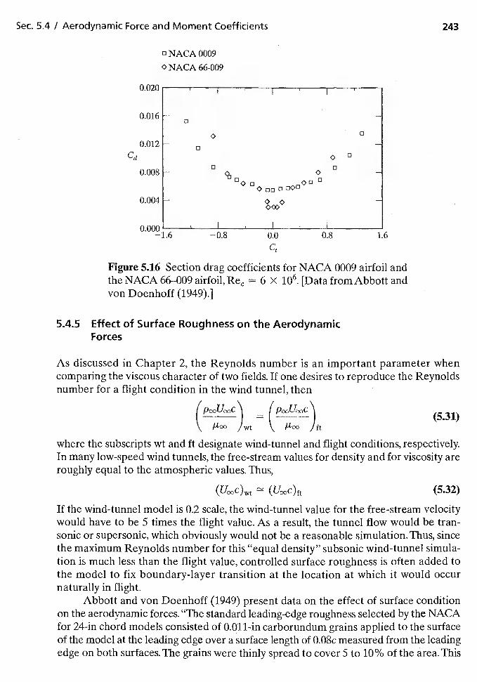
Sec. 54 / Aerodynamic Force and Moment Coefficients 243
ONACA 0009
O NACA 66-009
0.020
0.016ci
0 a
0.012—
Cd a
0,008- a
ODD0 00
0.004 -
0.000—1.6 —0.8 0.0 0.8 1.6
Cl
Figure 5.16 Section drag coefficients for NACA 0009 airfoil andthe NACA 66—009 airfoil, = 6 X 10⁶. [Data from Abbott andvon Doenhoff (1949).]
5.4.5 Effect of Surface Roughness on the AerodynamicForces
As discussed in Chapter 2, the Reynolds number is an important parameter whencomparing the viscous character of two fields. If one desires to reproduce the Reynoldsnumber for a flight condition in the wind tunnel, then
(5.31)\ /wt lit
where the subscripts wt and ft designate wind-tunnel and flight conditions, respectively.In many low-speed wind tunnels, the free-stream values for density and for viscosity areroughly equal to the atmospheric values. Thus,
(5.32)
If the wind-tunnel model is 0.2 scale, the wind-tunnel value for the free-stream velocitywould have to be 5 times the flight value. As a result, the tunnel flow would be tran-sonic or supersonic, which obviously would not be a reasonable simulation. Thus, sincethe maximum Reynolds number for this "equal density" subsonic wind-tunnel simula-tion is much less than the flight value, controlled surface roughness is often added tothe model to fix boundary-layer transition at the location at which it would occurnaturally in flight.
Abbott and von Doenhoff (1949) present data on the effect of surface conditionon the aerodynamic forces. "The standard leading-edge roughness selected by the NACAfor 24-in chord models consisted of 0.011-in carborundum grains applied to the surfaceof the model at the leading edge over a surface length of 0.08c measured from the leadingedge on both surfaces. The grains were thinly spread to coverS to 10% of the área.This
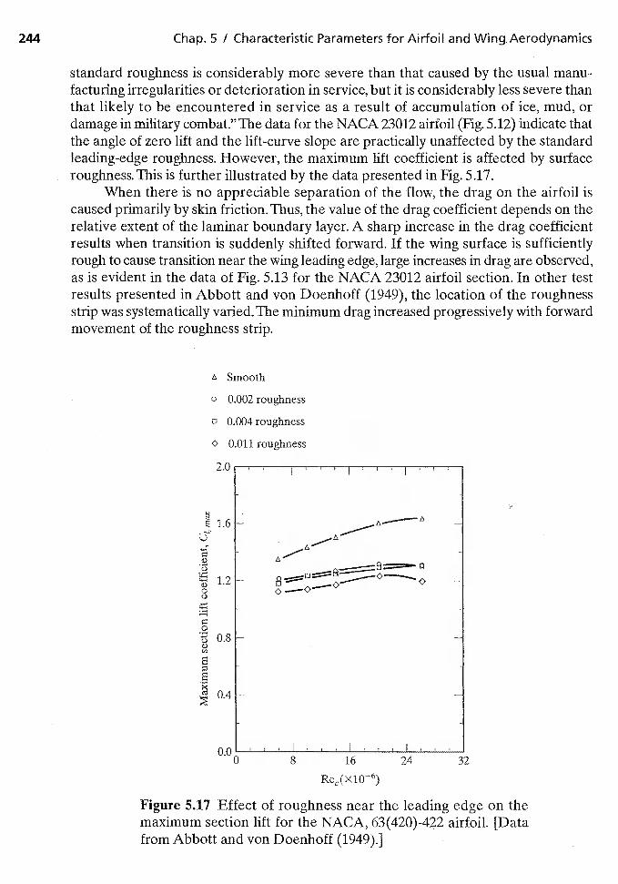
244 Chap. 5 / Characteristic Parameters for Airfoil and Wing Aerodynamics
standard roughness is considerably more severe than that caused by the usual manu-facturing irregularities or deterioration in service, but it is considerably less severe thanthat likely to be encountered in service as a result of accumulation of ice, mud, ordamage in military combat." The data for the NACA 23012 airfoil (Fig. 5.12) indicate thatthe angle of zero lift and the lift-curve slope are practically unaffected by the standardleading-edge roughness. However, the maximum lift coefficient is affected by surfaceroughness. This is further illustrated by the data presented in Fig. 5.17.
When there is no appreciable separation of the flow, the drag on the airfoil iscaused primarily by skin friction. Thus, the value of the drag coefficient depends on therelative extent of the laminar boundary layer. A sharp increase in the drag coefficientresults when transition is suddenly shifted forward. If the wing surface is sufficientlyrough to cause transition near the wing leading edge, large increases in drag are observed,as is evident in the data of Fig. 5.13 for the NACA 23012 airfoil section. In other testresults presented in Abbott and von Doenhoff (1949), the location of the roughnessstrip was systematically varied. The minimum drag increased progressively with forwardmovement of the roughness strip.
Smooth
o 0.002 roughness
o 0.004 roughness
O 0.011 roughness
I I I
16 —
1.2 -
00.8 -
I I I
0 8 16 24 32
Figure 5.17 Effect of roughness near the leading edge on themaximum section lift for the NACA, 63(420)-422 airfoil. [Datafrom Abbott and von Doenhoff (1949).]
Sec. 5.4 / Aerodynamic Force and Moment Coeffidents 245
Scaling effects between model simulations and flight applications (as they relateto the viscous parameters) are especially important when the flow field includes aninteraction between a shock wave and the boundary layer. The transonic flow field foran airfoil may include a shock-induced separation, a subsequent reattachment to theairfoil surface, and another boundary-layer separation near the trailing edge. Accordingto Pearcey, et al. (1968), the prime requirements for correct simulation of these tran-sonic shock/boundary-layer interactions include that the boundary layer is turbulent atthe point of interaction and that the thickness of the turbulent boundary layer for themodel flow is not so large in relation to the full-scale flow that a rear separation wouldoccur in the simulation that would not occur in the full-scale flow.
Braslow, et a!. (1966) provide some general guidelines for the use of grit-typeboundary-layer transition trips. Whereas it is possible to fix boundary-layer transition farforward on wind-tunnel models at subsonic speeds using grit-type transition tripsing little or no grit drag, the roughness configurations that are required to fix transitionin a supersonic flow often cause grit drag. Fixing transition on wind-tunnel models becomesincreasingly difficult as the Mach number is increased. Since roughness heights severaltimes larger than the boundary-layer thickness can be required to fix transition in ahypersonic flow, the required roughness often produces undesirable distortions of theflow. Sterret, et al. (1966) provides some general guidelines for the use of boundary-layer trips for hypersonic flows. Data are presented to illustrate problems that can arisefrom poor trip designs.
The comments regarding the effects of surface roughness were presented for tworeasons. (1) The reader should note that, since it is impossible to match the Reynolds num-ber in many scale-model simulations, surface roughness (in the form of boundary-layertrips) is often used to fix transition and therefore the relative extent of the laminar bound-ary layer. (2) When surface roughness is used, considerable care should be taken to prop-erly size and locate the roughness elements in order to properly simulate the desired flow.
The previous discussion in this section has focused on the effects of roughnesselements that have been intentionally placed on the surface to fix artificially the loca-tion of transition. As discussed, the use of boundary-layer trips is intended to compen-sate for the inability to simulate the Reynolds number in ground-test facilities. However,surface roughness produced by environmental "contamination" may have a significant(and unexpected) effect on the transition location. As noted by van Dam and Holmes(1986), loss of laminar flow can be caused by surface contamination such as insect debris,ice crystals, moisture due to mist or rain, surface damage, and "innocent" modificationssuch as the addition of a spanwise paint stripe.
As noted by van Dam and Holmes (1986), "The surface roughness caused by suchcontamination can lead to early transition near the leading edge. A turbulent boundarylayer which originates near the leading edge of an airfoil, substantially ahead of thepoint of minimum pressure, will produce a thicker boundary layer at the onset of thepressure recovery as compared to the conditions produced by a turbulent boundarylayer which originates further downstream. With sufficiently steep pressure gradientsin the recovery region, a change in the turbulent boundary layer conditions ... can leadto premature turbulent separation ..., thus affecting the aerodynamic characteristicsand the effectiveness of trailing-edge control surfaces. .. Also, forward movement oftransition location and turbulent separation produce a large increase in section drag."
246 Chap. 5 I Characteristic Parameters for Airfoil and Wing Aerodynamics
5.4.6 Method for Predicting Aircraft Parasite Drag
As you can imagine, total aircraft parasite drag is a complex combination of aircraftconfiguration, skin friction, pressure distribution, interference among aircraft compo-nents, and flight conditions (among other things). Accurately predicting parasite dragwould seem an a]most impossible task, especially compared with predicting lift.To makematters even more difficult, there are a variety of terms associated with drag, all of whichadd confusion about drag and predicting drag. Some of the common terms used todescribe drag are [Mccormick (1979)11:
• Induced (or vortex) drag—drag due to the trailing vortex system
• Skin friction drag—due to viscous stress acting on the surface of the body
• Form (or pressure) drag—due to the integrated pressure acting on the body, causedby flow separation
• Interference drag—due to the proximity of two (or more) bodies (e.g., wing andfuselage)
• Trim drag—due to aerodynamic forces required to trim the airplane about thecenter of gravity
• Profile drag—the sum of skin-friction and pressure drag for an airfoil section
• Parasite drag—the sum of skin-friction and pressure drag for an aircraft
• Base drag—the pressure drag due to a blunt base or afterbody
• Wave drag—due to shockwave energy losses
In spite of these complexities, numerous straightforward estimation methods exist forpredicting the parasite drag of aircraft, most of which use a combination of theoretical,empirical, and semi-empirical approaches.
While the building block methods for predicting skin-friction drag have beenpresented in Section 4.7.1 and 5.4.3, there are a variety of methods for applying skin-friction prediction methods to determine total aircraft drag. Every aerodynamicsgroup at each aircraft manufacturer has different methods for estimating subsonicaircraft drag. The basic approaches, however, are probably quite similar:
1. Estimate an equivalent flat-plate skin-friction coefficient for each component ofthe aircraft (wing, fuselage, stabilizers, etc.)
2. correct the skin-friction coefficient for surface roughness
3. Apply a form factor correction to each component's skin-friction coefficient totake into account supervelocities (velocities greater than free stream around thecomponent) as well as pressure drag due to flow separation to obtain a parasite-drag coefficient
4. convert each corrected skin-friction coefficient into an aircraft drag coefficientfor that component
5. Sum all aircraft parasite-drag coefficients to obtain a total aircraft drag coefficient
Sec. .4 I Aerodynamic Force and Moment Coefficients 247
Of course, this approach does not take into account a variety of sources of aircraft drag,including:
• Interference drag• Excrescence drag (the drag due to various small drag-producing protuberances,
including rivets, bolts, wires, etc.)
• Engine installation drag
• Drag due to control surface gaps
• Drag due to fuselage upsweep
• Landing gear drag
The total aircraft drag coefficient is defined as
__
DfCD = (5.33)
where is usually the wing planform area for an airplane. When the airplane dragcoefficient is 'defined in this way, the term "drag count" refers to a drag coefficient ofCD = 0.0001 (a drag cOefficient of CD = 0.0100 would be 100 drag counts); many aero-dynamicists refer to drag counts rather than the drag coefficient.
The following approach to determining subsonic aircraft parasite drag is due toShevell (1989) and also is presented in Schaufele (2000). This approach assumes thateach component of the aircraft contributes to the total drag without interfering witheach other. While this is not true, the approach provides a good starting point for theestimation of drag. The zero-lift drag coefficient for subsonic flow is obtained by:
N KiC1.Swet,CD0 = (5.34)
i1where N is the total number of aircraft components making up the aircraft (wing, fuse-lage, stabilizers, nacelles, pylons, etc.), is the form factor for each component, is thetotal skin-friction coefficient for each component, Swet. is the wetted area of each com-ponent, afld Srei is the aircraft reference area (there is only one reference area for theentire aircraft, which is usually the wing planform area).
Most aircraft components fall into one of two geometric categories: (1) wing-likeshapes and (2) body-like shapes. Because of this, there are two basic ways to find theequivalent flat-plate skin-friction coefficient for the various aircraft components.
Wing Method. A wing with a trapezoidal planform (as shown in Fig. 5.18) canbe defined by a root chord Cr, a tip chord a leading-edge sweep A, and a semi-span,b/2.The difficulty comes in applying the flat-plate skin-friction analysis to a wing with vari-able chord lengths along the span. Since the total skin-friction coefficient is a function ofthe Reynolds number at the "end of the plate", each spanwise station would have adifferent Reynolds number, and hence, a different total skin-friction coefficient.
It would be possible to perform a double integration along the chord and span ofthe wing to obtain a total skin-friction coefficient for the wing, however, an easier approach
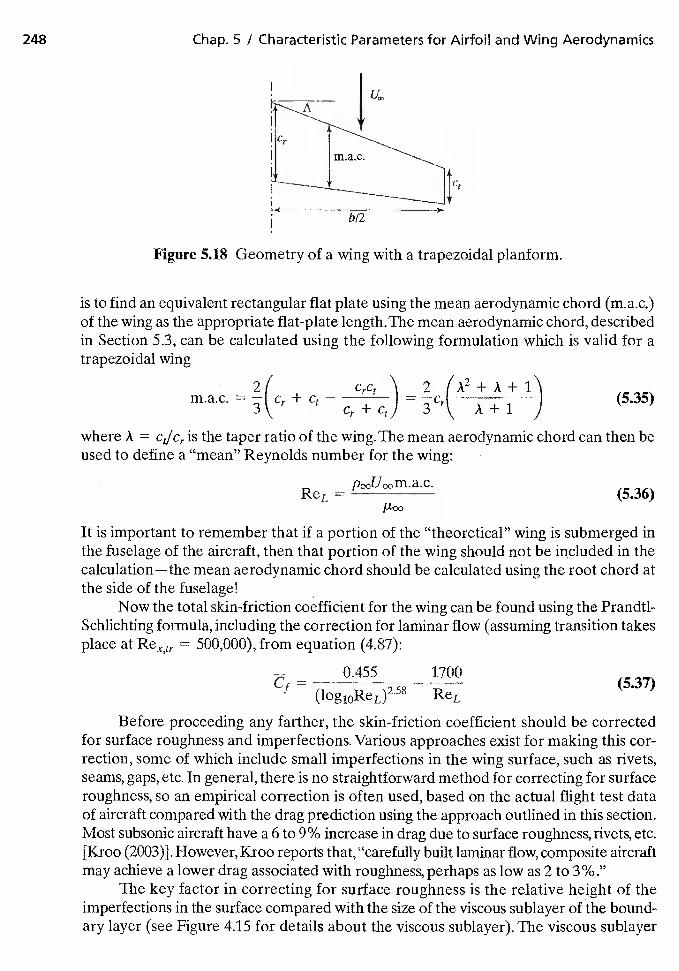
248 Chap. 5 / Characteristic Parameters for Airfoil and Wing Aerodynamics
Figure 5.18 Geometry of a wing with a trapezoidal planform.
is to find an equivalent rectangular flat plate using the mean aerodynamic chord (m.a.c.)of the wing as the appropriate flat-plate length. The mean aerodynamic chord, describedin Section 5.3, can be calculated using the following formulation which is valid for atrapezoidal wing
21 CrCt \ 2 (A2+A+1\m.a.c. = I Cr + Ct 1 = 1 (535)3\ Cr+CtJ 3 j
where A = Ct/Cr is the taper ratio of the wing. The mean aerodynamic chord can then beused to define a "mean" Reynolds number for the wing:
ReL = (5.36)
It is important to remember that if a portion of the "theoretical" wing is submerged inthe fuselage of the aircraft, then that portion of the wing should not be included in thecalculation mean aerodynamic chord should be calculated using the root chord atthe side of the fuselage!
Now the total skin-friction coefficient for the wing can be found using the Prandtl-Schlichting formula, including the correction for laminar flow (assuming transition takesplace at = 500,000), from equation (4.87):
— 0.455 1700C1 = — (5.37)
ReL
Before proceeding any farther, the skin-friction coefficient should be correctedfor surface roughness and imperfections. Various approaches exist for making this cor-rection, some of which include small imperfections in the wing surface, such as rivets,seams, gaps, etc. In general, there is no straightforward method for correcting for surfaceroughness, so an empirical correction is often used, based on the actual flight test dataof aircraft compared with the drag prediction using the approach outlined in this section.Most subsonic aircraft have a 6 to 9% increase in drag due to surface roughness, rivets, etc.{Kroo (2003)]. However, Kroo reports that, "carefully built laminar flow, composite aircraftmay achieve a lower drag associated with roughness, perhaps as low as 2 to 3%."
The key factor in correcting for surface roughness is the relative height of theimperfections in the surface compared with the size of the viscous sublayer of the bound-ary layer (see Figure 4.15 for details about the viscous sublayer). The viscous sublayer
b12
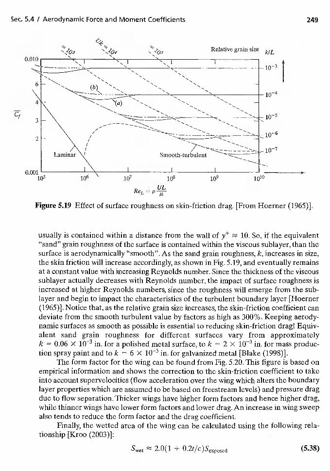
Sec. 5.4 / Aerodynamic Force and Moment Coefficients 249
I
10—6
1010
Figure 5.19 Effect of surface roughness on skin-friction drag. [From Hoerner (1965)].
usually is contained within a distance from the wall of 10. So, if the equivalent"sand" grain roughness of the surface is contained within the viscous sublayer, than thesurface is aerodynamically "smooth". As the sand grain roughness, k, increases in size,the skin friction will increase accordingly, as shown in Fig. 5.19, and eventually remainsat a constant value with increasing Reynolds number. Since the thickness of the viscoussublayer actually decreases with Reynolds number, the impact of surface roughness isincreased at higher Reynolds numbers, since the roughness will emerge from the sub-layer and begin to impact the characteristics of the turbulent boundary layer [Hoerner(1965)]. Notice that, as the relative grain size increases, the skin-friction coefficient candeviate from the smooth turbulent value by factors as high as 300%. Keeping aerody-namic surfaces as smooth as possible is essential to reducing skin-friction drag! Equiv-alent sand grain roughness for different surfaces vary from approximatelyk = 0.06 x in. for a polished metal surface, to k = 2 X in. for mass produc-tion spray paint and to k = 6 X in. for galvanized metal [Blake (1998)}.
The form factor for the wing can be found from Fig. 5.20. This figure is based onempirical information and shows the correction to the skin-friction coefficient to takeinto account supervelocities (flow acceleration over the wing which alters the boundarylayer properties which are assumed to be based on freestream levels) and pressure dragdue to flow separation. Thicker wings have higher form factors and hence higher drag,while thinner wings have lower form factors and lower drag. An increase in wing sweepalso tends to reduce the form factor and the drag coefficient.
Finally, the wetted area of the wing can be calculated using the following rela-tionship [Kroo (2003)]:
Swet 2.0(1 + O.2t/C)Sexposed (5.38)
0.010
Relative grain size kIL
0.001
ULReL = P
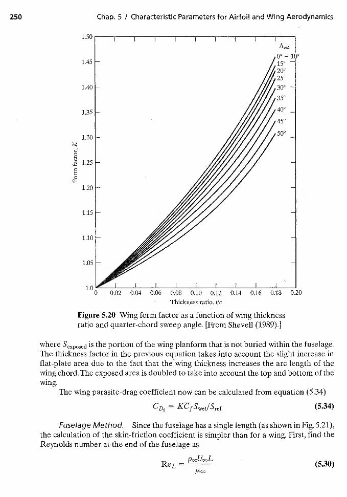
CD0 = KCfSwet/Sref
I I I
0° — 100
15° —20°25°
1.35 -
1.30 -
1.25-
40°
,450
50°
1.20 -
250 Chap. 5 / Characteristic Parameters for Airfoil and Wing Aerodynamics
1,50
1.45
1,40 -
00
EI-,0
1.15 -
1.10
1.05
100 0.20
Figure 5.20 Wing form factor as a function of wing thicknessratio and quarter-chord sweep angle. [From Shevell (1989).]
where Sexposed is the portion of the wing planform that is not buried within the fuselage.The thickness factor in the previous equation takes into account the slight increase inflat-plate area due to the fact that the wing thickness increases the arc length of thewing chord.The exposed area is doubled to take into account the top and bottom of thewing.
The wing parasite-drag coefficient now can be calculated from equation (5.34)
(5.34)
Fuselage Method. Since the fuselage has a single length (as shown in Fig. 5.21),the calculation of the skin-friction coefficient is simpler than for a wing. First, find theReynolds number at the end of the fuselage as
ReL = (5.30)
0.02 0.04 0.06 0.08 0.10 0.12 0.14 0.16 0.18
Thickness ratio, tic
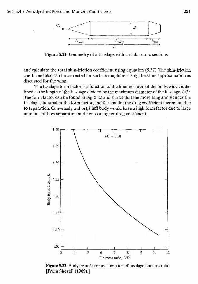
Sec. 5.4 I Aerodynamic Force and Moment Coefficients
I..0U
g
0
251
ID'•
L
Figure 5.21 Geometry of a fuselage with circular cross sections.
and calculate the total skin-friction coefficient using equation (5.37). The skin-frictioncoefficient also can be corrected for surface roughness using the same approximation asdiscussed for the wing.
The fuselage form factor is a function of the fineness ratio of the body, which is de-fmed as the length of the fuselage divided by the maximum diameter of the fuselage, LID.The form factor can be found in Fig. 5.22 and shows that the more long and slender thefuselage, the smaller the form factor, and the smaller the drag coefficient increment dueto separation. Conversely, a short, bluff body would have a high form factor due to largeamounts of flow separation and hence a hither drag coefficient.
1.40 —
1.35 -
1.30 -
1.25 -
1.20
1.15 —
1.10 -
1.05
1 I I
= 0.50
I I I I —
3 4 5 6 7 8 9 10 11
Fineness ratio, LID
Figure 5.22 Body form factor as a function of fuselage fineness ratio.[From Shevell (1989).]
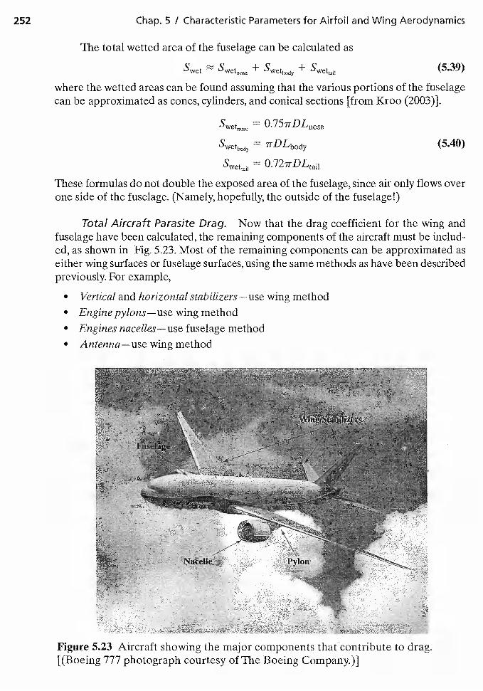
252 Chap. 5 I Characteristic Parameters for Airfoil and Wing Aerodynamics
The total wetted area of the fuselage can be calculated as
+ Swet + Swet (5.39)
where the wetted areas can be found assuming that the various portions of the fuselagecan be approximated as cones, cylinders, and conical sections [from Kroo (2003)].
Swet = O.75lrDLnose
lrDLbody (5.40)
O.72lrDLtaii
These formulas do not double the exposed area of the fuselage, since air only flows overone side of the fuselage. (Namely, hopefully, the outside of the fuselage!)
Total Aircraft Parasite Drag. Now that the drag coefficient for the wing andfuselage have been calculated, the remaining components of the aircraft must be includ-ed, as shown in Fig. 5.23. Most of the remaining components can be approximated aseither wing surfaces or fuselage surfaces, using the same methods as have been describedpreviously. For example,
• Vertical and horizontal stabilizers — use wing method• Engine pylons—use wing method• Engines nacelles —use fuselage method• Antenna—use wing method
Figure 5.23 Aircraft showing the major components that contribute to drag.[(Boeing 777 photograph courtesy of The Boeing Company.)]
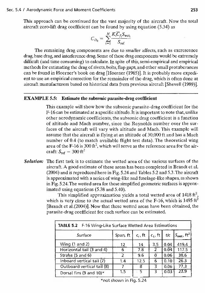
Sec. 5.4 / Aerodynamic Force and Moment Coefficients 253
This approach can be continued for the vast majority of the aircraft. Now the totalaircraft zero-lift drag coefficient can be found by using equation (5.34) as
N KiCfSwet.
i=1
The remaining drag components are due to smaller affects, such as excrescencedrag, base drag, and interference drag. Some of these drag components would be extremelydifficult (and time consuming) to calculate. In spite of this, semi-empirical and empiricalmethods for estimating the drag of rivets, bolts, flap gaps, and other small protuberancescan be found in Hoerner's book on drag [Hoerner (1965)]. It is probably more expedi-ent to use an empirical correction for the remainder of the drag, which is often done ataircraft manufacturers based on historical data from previous aircraft [Shevell (1989)].
EXAMPLE 5.5: Estimate the subsonic parasite-drag coefficient
This example will show how the subsonic parasite-drag coefficient for theF-16 can be estimated at a specific altitude. It is important to note that, unlikeother aerodynamic coefficients, the subsonic drag coefficient is a functionof altitude and Mach number, since the Reynolds number over the sur-faces of the aircraft will vary with altitude and Mach. This example willassume that the aircraft is flying at an altitude of 30,000 ft and has a Machnumber of 0.4 (to match available flight test data). The theoretical wingarea of the F-16 is 300 ft2, which will serve as the reference area for the air-craft: Sref = 300 ft2
Solution: The first task is to estimate the wetted area of the various surfaces of theaircraft. A good estimate of these areas has been completed in Brandt et al.(2004) and is reproduced here in Fig. 5.24 and Tables 5.2 and 5.3.The aircraftis approximated with a series of wing-like and fuselage-like shapes, as shownin Fig. 5.24. The wetted area for these simplified geometric surfaces is approx-imated using equations (5.38 and 5.40).
This simplified approximation yields a total wetted area of 1418 ft2,which is very close to the actual wetted area of the F-16, which is 1495 ft2[Brandt et al.(2004)]. Now that these wetted areas have been obtained, theparasite-drag coefficient for each surface can be estimated.
TABLE 5.2 F-16 Wing-Like Surface Wetted Area Estimations
Surface Span, ft Cr, ft Ct, ft tic 112
Wing (1 and 2) '12 14 3.5 0.04 419.4Horizontal tail (3 and 4) 6 7.8 2 0.04 117.5
Strake (5 and 6) 2 9.6 0 0.06 38.6Inboard vertical tail (7) '1.4 12.5 6 0.10 26.3
Outboard vertical tail (8) 7 8 3 0.06 77.3
Dorsal fins (9 and 1O)* 1.5 5 3 23.9
*not snown in Fig. 5.24
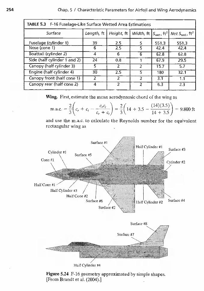
254 Chap. 5 / Characteristic Parameters for Airfoil and Wing Aerodynamics
TABLE 5,3 F-16 Fuselage-Like Surface Wetted Area Estimations
Surface Length, ft Height, ft width, ft 5wet, ft2 Net ft2
Fuselage (cylinder 1) 39 2.5 5 551.3 551.3Nose (cone 1) 6 2.5 5 42.4 42.4Boattail (cylinder 2) 4 6 6 62.8 62.8Side (half cylinder 1 and 2) 24 0.8 1 67.9 29.5Canopy(halfcylinder3) 5 2 2 15.7 5.7
Engine (half cylinder4) 30 2.5 5 180 32.1
Canopyfront(half cone 1) 2 2 2 3.1 1.1
Canopy rear (half cone 2) 4 2 2 6.3 2.3
Wing. First, estimate the mean aerodynamic chord of the wing as
21 cc \ 2/ (14)(3.5)\TI 1(14+353\\ 3\ 14+3.5)
and use the m.a,c. to calculate the Reynolds number for the equivalentrectangular wing as
Surface #3
VCylinder #2
Half Cylinder #2 Surface #4
Figure 5.24 F-16 geometry approximated by simple shapes.[From Brandt et al. (2004).I
Half Cylinder #1Surface #1
Cylinder #1Surface #5
Cone #1
Half Cone #1
Half Cylinder #3
Half Cone #2#6
Surface #2
Surface #8
Surface #7
Half Cylinder #4
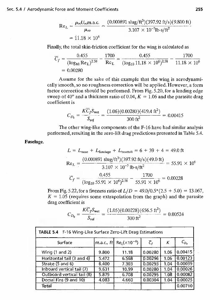
Sec. 5.4 / Aerodynamic Force and Moment Coefficients 255
(0.000891 slug/ft3)(397.92 ft/s)(9.800 ft)ReL= —
1107 X
= 11.18 X 10⁶
Finally, the total skin-friction coefficient for the wing is calculated as
— 0.455 1700 0.455 1700Cf
— (log10 ReL)258 — ReL — (log10 11.18 X 10⁶)2.58 — 11.18 X
= 0.00280
Assume for the sake of this example that the wing is aerodynami-cally smooth, so no roughness correction will be applied. However, a formfactor correction should be performed. From Fig. 5.20, for a leading edgesweep of 40° and a thickness ratio of 0.04, K 1.06 and the parasite dragcoefficient is
KCfSwet (1.06)(0.00280)(419.4 ft2)CD = = =0.00415
o
5ref 300 ft2
The other wingLlike components of the F-16 have had similar analysisperformed, resulting in the zero-lift drag predictions presented in Table 5.4.
Fuseiage.
L = Lnose + + Lboattail 6 + 39 + 4 = 49.0 ft
(0.000891 slug/ft3) (397.92 ft/s)(49.0 ft)ReL = = 55.91 ><
3.107 X lb-s/ft2
— 0.455 1700Cf = — = 0.00228
(log10 55.91 X 10⁶)2.58 55.91 X
From ratio of L/D = 49.0/0.5*(2.5 + 5.0) = 13.067,K = 1.05 (requires some extrapolation from the graph) and the parasitedrag coefficient is
KCfSwet (1.05)(0.00228) (656.5 ft2)CD = = 0.00524
Sref 300 ft2
TABLE 5.4 F-16 Wing-Like Surface Zero-Lift Drag Estimations
Surface m.a.c., ft ReL(x106) Cf K C00
Wing (1 and 2) 9.800 11.18 0.00280 1.06 0.00415
Horjzontal tail (3 and 4) 5.472 6.568 0.00296 1.06 0.00123Strake (5 and 6) 6.400 7.303 0.00293 1.04 0.00039Inboard vertical tail (7) 9.631 10.99 0.00280 1.04 0.00026Outboard vertical tail (8) 5.879 6.708 0.00295 1.08 0.00082Dorsal Fins (9 and 4.083 4.660 0.00304 1.04 0.00025Total 0.00710
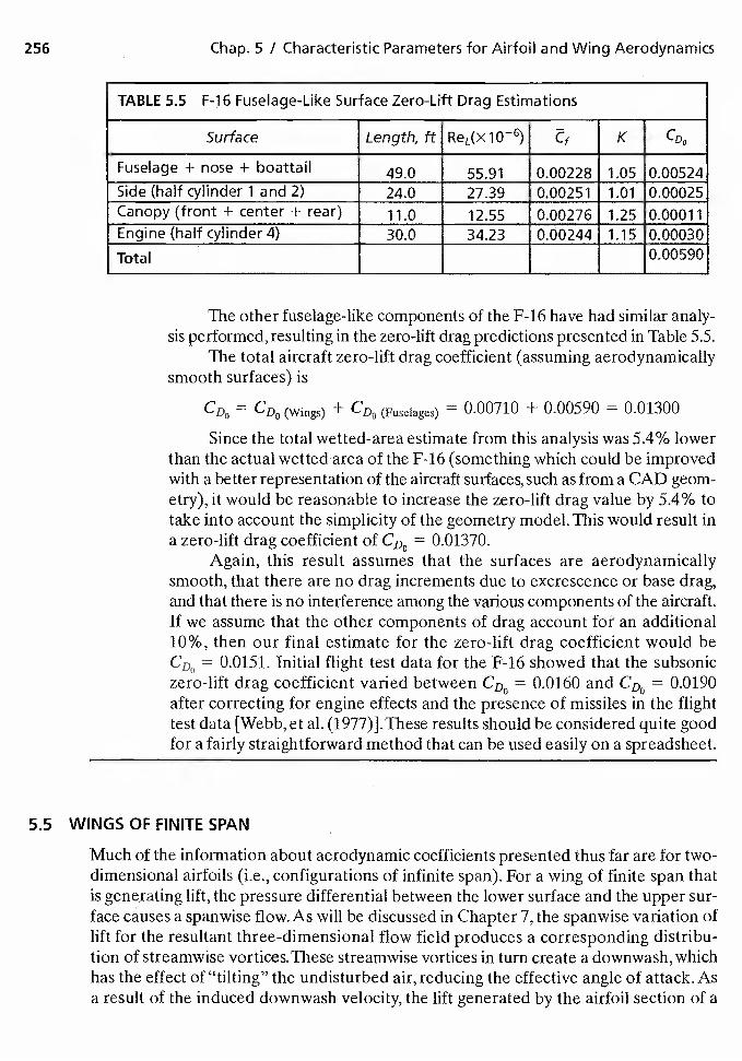
256 Chap. 5 / Characteristic Parameters for Airfoil and Wing Aerodynamics
TABLE 5.5 F-16 Fuselage-Like Surface Zero-Lift Drag Estimations
Surface Length, ft ReL(X106) K CD0
Fuselage + nose + boattail 49.0 55.91 0.00228 1.05 0.00524Side (half cylinder 1 and 2) 24.0 27.39 0.00251 1.01 0.00025Canopy (front + center + rear) 11.0 12.55 0.00276 1.25 0.00011Engine (half cylinder 4) 30.0 34.23 0.00244 1.15 0.00030
Total 0.00590
The other fuselage-like components of the F-16 have had similar analy-sis performed, resulting in the zero-lift drag predictions presented in Table 5.5.
The total aircraft zero-lift drag coefficient (assuming aerodynamicallysmooth surfaces) is
CD0 CD0 (Wings) + CD0 (Fuselages) = 0.00710 + 0.00590 = 0.01300
Since the total wetted-area estimate from this analysis was 5.4% lowerthan the actual wettedarea of the F-16 (something which could be improvedwith a better representation of the aircraft surfaces, such as from a CAD geom-etry), it would be reasonable to increase the zero-lift drag value by 5.4% totake into account the simplicity of the geometry model.This would result ina zero-lift drag coefficient of CD0 = 0.01370.
Again, this result assumes that the surfaces are aerodynamicallysmooth, that there are drag increments due to excrescence or base drag,and that there is no interference among the various components of the aircraft.If we assume that the other components of drag account for an additional10%, then our final estimate for the zero-lift drag coefficient would beCD0 = 0.0151. Initial flight test data for the F-16 showed that the subsoniczero-lift drag coefficient varied between CD0 = 0.0160 and CD0 = 0.0190after correcting for engine effects and the presence of missiles in the flighttest data [Webb, et al. (1977)].These results should be considered quite goodfor a fairly straightforward method that can be used easily on a spreadsheet.
5.5 WINGS OF FINITE SPAN
Much of the infonnation about aerodynamic coefficients presented thus far are for two-dimensional airfoils (i.e., configurations of infinite span). For a wing of finite span thatis generating lift, the pressure differential between the lower surface and the upper sur-face causes a spanwise flow. As will be discussed in Chapter 7, the spanwise variation oflift for the resultant three-dimensional flow field produces a corresponding distribu-tion of streamwise vortices.These streamwise vortices in turn create a downwash, whichhas the effect of "tilting" the undisturbed air, reducing the effective angle of attack. Asa result of the induced downwash velocity, the lift generated by the airfoil section of a
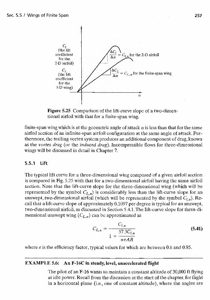
Sec. 5.5 / Wings of Finite Span 257
Cl(the lift
coefficientfor the
2-D airfoil)
CL(the lift wing
coefficientfor the
3-D wing)
Figure 5.25 Comparison of the lift-curve slope of a two-dimen-sional airfoil with that for a finite-span wing.
finite-span wing which is at the geometric angle of attack a is less than that for the sameairfoil section of an infinite-span airfoil configuration at the same angle of attack. Fur-thermore, the trailing vortex system produces an additional component of drag, knownas the vortex drag (or the induced drag). Incompressible flows for three-dimensionalwings will be discussed in detail in Chapter 7.
5.5.1 Lift
The typical lift curve for a three-dimensional wing composed of a given airfoil sectionis compared in Fig, 5.25 with that for a two-dimensional airfoil having the same airfoilsection. Note that the lift-curve slope for the three-dimensional wing (which will berepresented by the symbol CLif) is considerably less than the lift-curve slope for anunswept, two-dimensional airfoil (which will be represented by the symbol C/,if). Re-call that a lift-curve slope of approximately 0.1097 per degree is typical for an unswept,two-dimensional airfoil, as discussed in Section 5.4.1.The lift-curve slope for three-di-mensional unswept wing (CL,if) can be approximated as
C/if
= 57.3c1(5.41)
1+ireAR
where e is the efficiency factor, typical values for which are between 0.6 and 0.95.
EXAMPLE 5.6: An F-16C in steady, level, unaccelerated flight
The pilot of an F-16 wants to maintain a constant altitude of 30,000 ft flyingat idle power. Recall from the discussion at the start of the chapter, for flightin a horizontal plane (i.e., one of constant altitude), where the angles are
for the 2-D airfoil
a
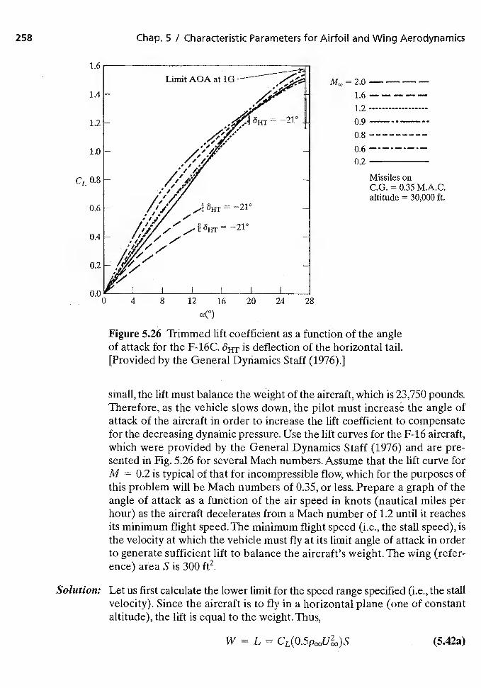
Figure 5.26 Trimmed lift coefficient as a function of the angleof attack for the F-16C, 6HT is deflection of the horizontal tail.[Provided by the General Dynamics Staff (1976).]
small, the lift must balance the weight of the aircraft, which is 23,750 pounds.Therefore, as the vehicle slows down, the pilot must increase the angle ofattack of the aircraft in order to increase the lift coefficient to compensatefor the decreasing dynamic pressure. Use the lift curves for the F-16 aircraft,which were provided by the General Dynamics Staff (1976) and are pre-sented in Fig. 5.26 for several Mach numbers. Assume that the lift curve forM = 0.2 is typical of that for incompressible flow, which for the purposes ofthis problem will be Mach numbers of 0.35, or less. Prepare a graph of theangle of attack as a function of the air speed in knots (nautical miles perhour) as the aircraft decelerates from a Mach number of 1.2 until it reachesits minimum flight speed. The minimum flight speed (i.e., the stall speed), isthe velocity at which the vehicle must fly at its limit angle of attack in orderto generate sufficient lift to balance the aircraft's weight. The wing (refer-ence) area S is 300 ft2.
Solution: Let us first calculate the lower limit for the speed range specified (i.e., the stallvelocity). Since the aircraft is to fly in a horizontal plane (one of constantaltitude), the lift is equal to the weight.Thus,
W = L = (5.42a)
1
1.
1.2
258 Chap. 5 / Characteristic Parameters for Airfoil and Wing Aerodynamics
M0. = 2.0 — — — —1.6
1.2
0.9—---————--
0.8
0.6 — - —. — — —
0.2
c Missiles onL C.G. = 0.35 M.A.C.
altitude = 30,000 ft.
0 4 8 12 16 20 24 28
a(°)
Sec. 5.5 I Wings of Finite Span 259
In order to compensate for the low dynamic pressure that occurs whenflying at the stall speed (Ustaii), the lift coefficient must be the maximumattainable value, CL Thus,
— r — r' IA ITT \2— —
Solving for Usta11,/2W
Ustati'I PooCi.,maxS
Referring to Fig. 5.26, the maximum value of the lift coefficient (assuming itoccurs at an incompressible flow condition) is 1.57, which corresponds to thelimit angle of attack. From Table 1.2b, the free-stream density at 30,000 ft is0.0008907 slugs/ft3, or 0.0008907 lbf s2/ft4. Thus,
— / 2(237501bf)stall
— (0.0008907 lbfs2/ft4)(1.57)(300ft2)
Ustaii = 336.5 ft/s = 199.2 knots
Thus, the minimum velocity at which the weight of the F-16 is balanced bythe lift at 30,000 ft is 199.2 knots with the aircraft at an angle of attack of27.50. The corresponding Mach number is
336.5 ft/s
= a 994.85 ft/s= 0.338
To calculate the lift coefficient as a function of Mach number from = 1.2
down to the stall value for the Mach number,
= 2W2
(5.42b)S
The velocity in knots is given by
=
where has the units of knots. The values obtained using these equationsand using the lift curves presented in Fig. 5.26 to determine the angle ofattack required to produce the required lift coefficient at a given Machnumber are presented in the following table.
(—)
CL
(—) (°)
Uc,c,
(ftls)Uco
(knots)
1.2 0.125 1.9 1193.82 706.80.9 0.222 2.4 895.37 530.10.8 0.281 3.5 795.88 471.20.6 0.499 6.2 596.91 353.40.338 1.57 27.5 336.50 199.2
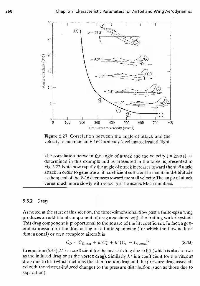
Figure 5.27 Correlation between the angle of attack and thevelocity to maintain an F-16C in steady, level unaccelerated flight.
The correlation between the angle of attack and the velocity (in knots), asdetermined in this example and as presented in the table, inFig. 5.27. Note how rapidly the angle of attack increases toward the stall angleattack in order to generate a lift coefficient sufficient to maintain the altitudeas the speed of the F-16 decreases toward the stall velocity. The angle of attackvaries much more slowly with velocity at transonic Mach numbers.
As noted at the start of this section, the three-dimensional flow past a finite-span wingproduces an additional component of drag associated with the trailing vortex system.This drag component is proportional to the square of the lift coefficient. In fact, a gen-eral expression for the drag acting on a finite-span wing (for which the flow is threedimensional) or on a complete aircraft is
— C + 'r2 + 5 43D,mrn "- '—L '—L,min)
In equation (5.43), k' is a coefficient for the inviscid drag due to lift (which is also knownas the induced drag or as the vortex drag). Similarly, k" is a coefficient for the viscousdrag due to lift (which includes the skin friction drag and the pressure drag associat-ed with the viscous-induced changes to the pressure distribution, such as those due toseparation).
260 Chap. S I Characteristic Parameters for Airfoil and Wing Aerodynamks
I)
0
00 100 200 300 400 500 600
Free-stream velocity (knots)700 800
5.52 Drag
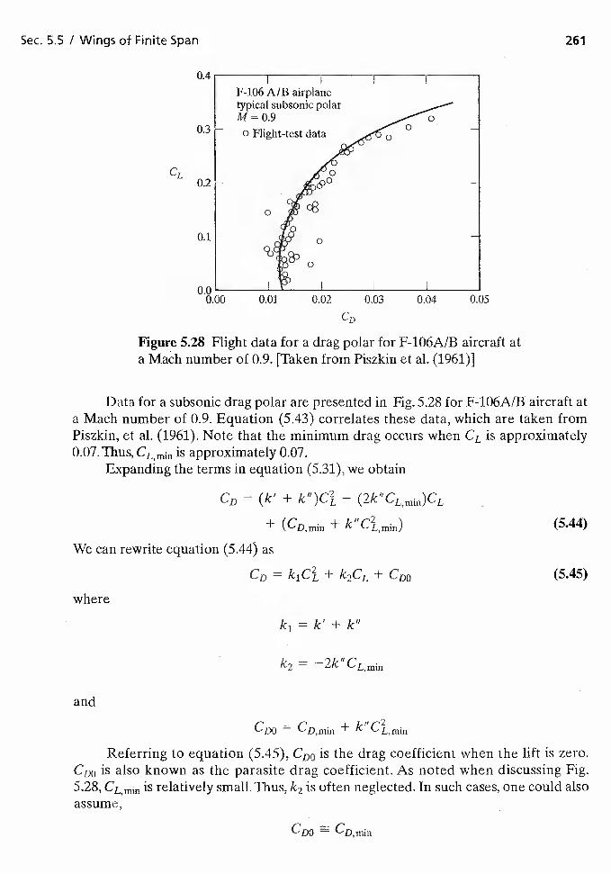
Sec. 5.5 I Wings of Finite Span 261
CL
0.4
0.3
0.2
0.1
0.00.00
Figure 5.28 Flight data for a drag polar for F-106A/B aircraft ata Mach number of 0.9. [Taken from Piszkin et al. (1961)]
Data for a subsonic drag poiar are presented in Fig. 5.28 for F-106A/B aircraft ata Mach number of 0.9. Equation (5.43) correlates these data, which are taken fromPiszkin, et a!. (1961). Note that the minimum drag occurs when CL is approximately0.07. Thus, CL mm is approximately 0.07.
Expanding the terms in equation (5.31), we obtain
CD = (k' + —
+ (CDmin +
We can rewrite equation (5.44) as
(5.44)
where
and
CD = k1C3. + k2CL + CDO
= k' + k"
I — "r"2 — '-"'
C —DO L,min
(5.45)
Referring to equation (5.45), CDO is the drag coefficient when the lift is zero.CDO is also known as the parasite drag coefficient. As noted when discussing Fig.5.28, CLmm is relatively small. Thus, k2 is often neglected. In such cases, one could alsoassume,
CDO CDrnin
0.01 0.02 0.03 0.04 0.05
CD
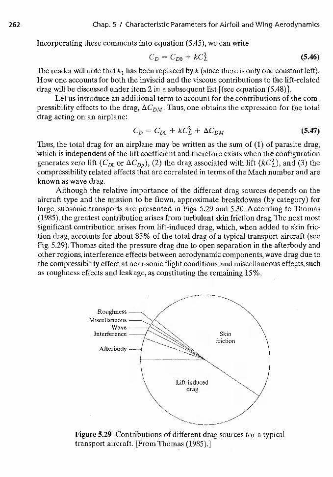
262 Chap. S / Characteristic Parameters for Airfoil and Wing Aerodynamics
Incorporating these comments into equation (5.45), we can write
CD + (5.46)
The reader will note that k1 has been replaced by k (since there is only one constant left).How one accounts for both the inviscid and the viscous contributions to the lift-relateddrag will be discussed under item 2 in a subsequent list [(see equation (5.48)].
Let us introduce an additional term to account for the contributions of the com-pressibility effects to the drag, Thus, one obtains the expression for the totaldrag acting on an airplane:
— + r''—DO
Thus, the total drag for an airplane may be written as the sum of (1) of parasite drag,which is independent of the lift coefficient and therefore exists when the configurationgenerates zero lift (CDO or (2) the drag associated with lift and (3) thecompressibility related effects that are correlated in terms of the Mach number and areknown as wave drag.
Although the relative importance of the different drag sources depends on theaircraft type and the mission to be flown, approximate breakdowns (by category) forlarge, subsonic transports are presented in Figs. 5.29 and 5.30. According to Thomas(1985), the greatest contribution arises from turbulent skin friction drag. The next mostsignificant contribution arises from lift-induced drag, which, when added to skin fric-tion drag, accounts for about 85% of the total drag of a typical transport aircraft (seeFig. 5.29). Thomas cited the pressure drag due to open separation in the afterbody andother regions, interference effects between aerodynamic components, wave drag due tothe compressibility effect at near-sonic flight conditions, and miscellaneous effects, suchas roughness effects and leakage, as constituting the remaining 15%.
RoughnessMiscellaneous
WaveInterference
Afterbody
Figure 5.29 Contributions of different drag sources for a typicaltransport aircraft. [From Thomas (1985).]
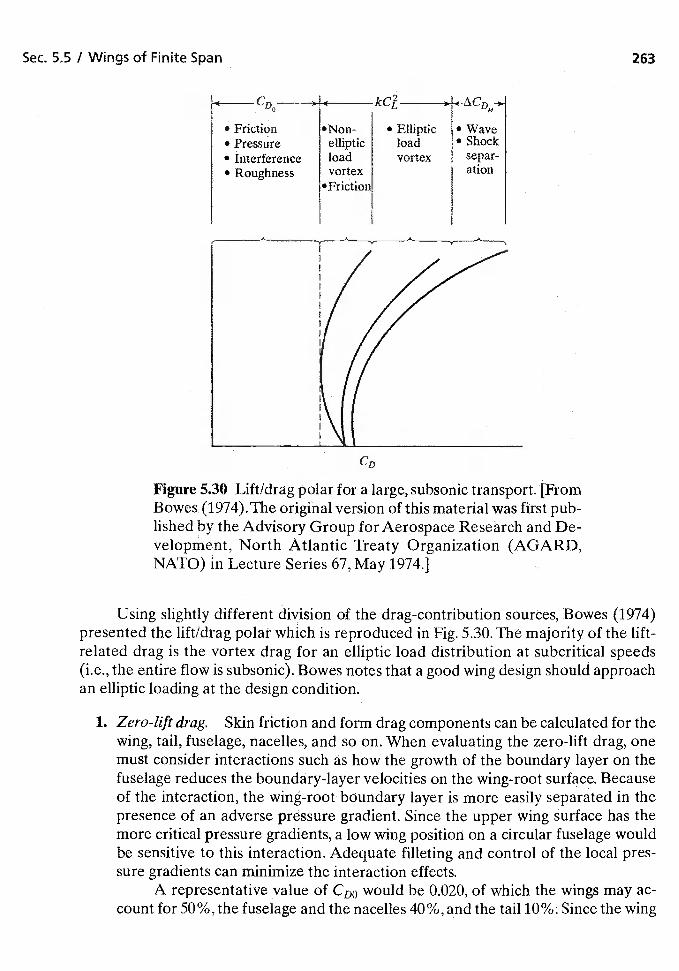
Sec. 5.5 I Wings of Finite Span 263
Figure 5.30 Lift/drag.polar for a large, subsonic transport. [FromBowes(1974).The original version of this material was first pub-lished by the Advisory Group for Aerospace Research and De-velopment, North Atlantic Treaty Organization (AGARD,NATO) in Lecture Series 67, May 1974.]
Using slightly different division of the drag-contribution sources, Bowes (1974)presented the lift/drag polar which is reproduced in Fig. 5.30. The majority of the lift-related drag is the vortex drag for an elliptic load distribution at subcritical speeds(i.e., the entire flow is subsonic). Bowes notes that a good wing design should approachan elliptic loading at the design condition.
1. Zero-lift drag. Skin friction and form drag components can be calculated for thewing, tail, fuselage, nacelles, and so on. When evaluating the zero-lift drag, onemust consider interactions such as how the growth of the boundary layer on thefuselage reduces the boundary-layer velocities on the wing-root surface. Becauseof the interaction, the wing-root boundary layer is more easily separated in thepresence of an adverse pressure gradient. Since the upper wing surface has themore critical pressure gradients, a low wing position on a circular fuselage wouldbe sensitive to this interaction. Adequate filleting and control of the local pres-sure gradients can minimize the interaction effects.
A representative value of CDO would be 0.020, of which the wings may ac-count for 50%, the fuselage and the nacelles 40%, and the tail 10%. Since the wing
• Friction• Pressure• Interference• Roughness
KLL
•Non- • Ellipticelliptic loadload vortexvortex
'Friction
• Wave• Shock
separ-ation
CL,
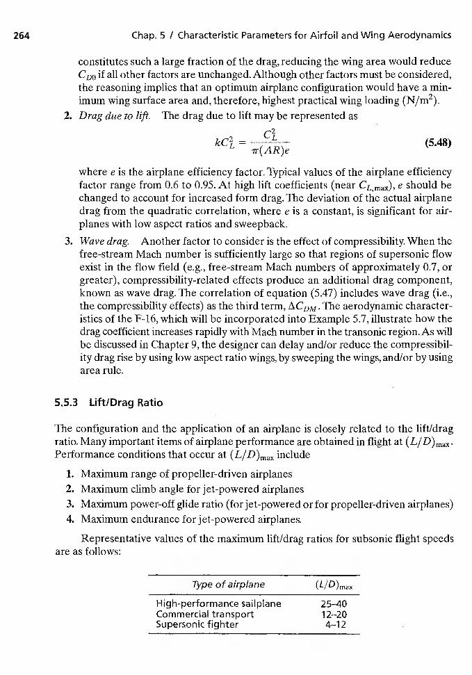
264 Chap. 5 / Characteristic Parameters for Airfoil and Wing Aerodynamics
constitutes such a large fraction of the drag, reducing the wing area would reduceCDO if all other factors are unchanged. Although other factors must be considered,the reasoning implies that an optimum airplane configuration would have a min-imum wing surface area and, therefore, highest practical wing loading (N/rn2).
2. Drag due to lift. The drag due to lift may be represented as
C2= L (548)'Tr(AR)e
where e is the airplane efficiency factor. Typical values of the airplane efficiencyfactor range from 0.6 to 0.95. At high lift coefficients (near CL,max), e should bechanged to account for increased form drag. The deviation of the actual airplanedrag from the quadratic correlation, where e is a constant, is significant for air-planes with low aspect ratios and sweepback.
3. Wave drag. Another factor to consider is the effect of compressibility. When thefree-stream Mach number is sufficiently large so that regions of supersonic flowexist in the flow field (e.g., free-stream Mach numbers of approximately 0.7, orgreater), compressibility-related effects produce an additional drag component,known as wave drag. The correlation of equation (5.47) includes wave drag (i.e.,the compressibility effects) as the third term, The aerodynamic character-istics of the F46, which will be incorporated into Example 5.7, illustrate how thedrag coefficient increases rapidly with Mach number in the transonic region. As willbe discussed in Chapter 9, the designer can delay and/or reduce the compressibil-ity drag rise by using low aspect ratio wings, by sweeping the wings, and/or by usingarea rule.
5.5.3 Lift/Drag Ratio
The configuration and the application of an airplane is closely related to the lift/dragratio. Many important items of airplane performance are obtained in flight atPerformance conditions that occur at (L/D)max include
1. Maximum range of propeller-driven airplanes2. Maximum climb angle for jet-powered airplanes3. Maximum power-off glide ratio (for jet-powered or for propeller-driven airplanes)4. Maximum endurance for jet-powered airplanes.
Representative values of the maximum lift/drag ratios for subsonic flight speedsare as follows:
Type of airplane (L/D)max
High-performance sailplane 25-40Commercial transportSupersonic fighter
12-204—12
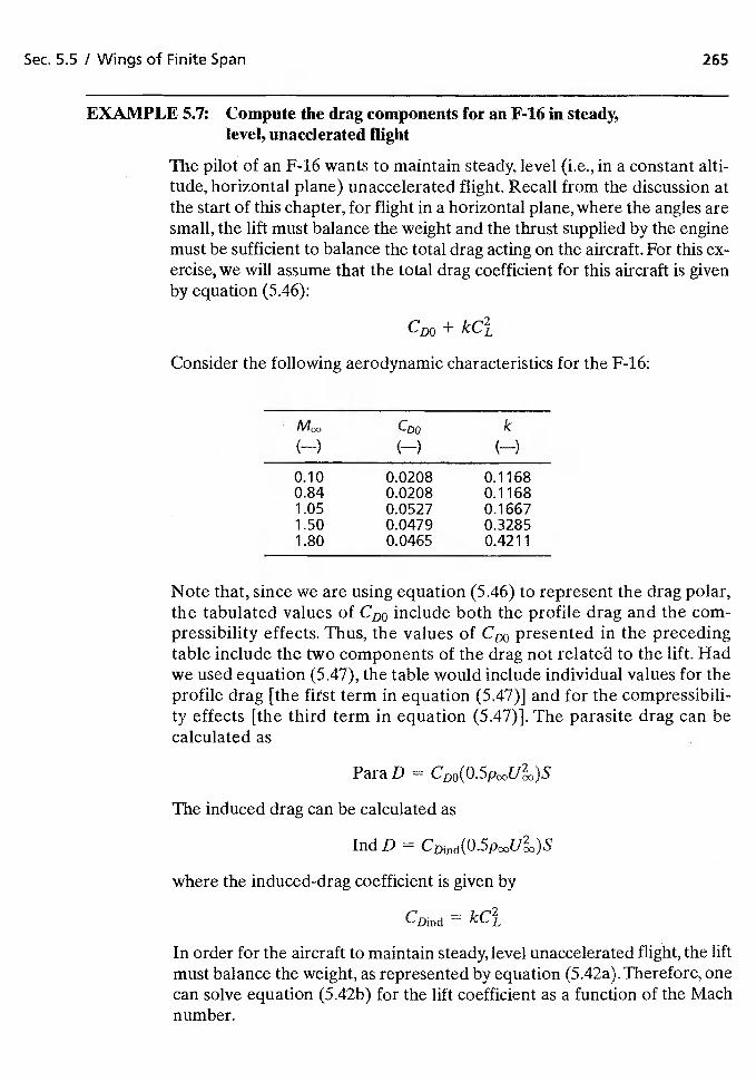
Sec. 5.5 / Wings of Finite Span 265
EXAMPLE 5.7: Compute the drag components for an F-16 in steady,level, unaccierated flight
The pilot of an F-16 wants to maintain steady, level (i.e., in a constant alti-tude, horizontal plane) unaccelerated flight. Recall from the discussion atthe start of this chapter, for flight in a horizontal plane, where the angles aresmall, the lift must balance the weight and the thrust supplied by the enginemust be sufficient to balance the total drag acting on the aircraft. For this ex-ercise, we will assume that the total drag coefficient for this aircraft is givenby equation (5.46):
ç00 +
Consider the following aerodynamic characteristics for the F-16:
(—)
C00
(—)
k(—)
0.10 0.0208 0.11680.84 0.0208 0.11681.05 0.0527 0.16671.50 0.0479 0.32851.80 0.0465 0.4211
Note that, since we are using equation (5.46) to represent the drag polar,the tabulated values of CDO include both the profile drag and the com-pressibility effects. Thus, the values of presented in the precedingtable include the two components of the drag not related to the lift. Hadwe used equation (5.47), the table would include individual values for theprofile drag [the first term in equation (5.47)] and for the compressibili-ty effects [the third term in equation (5.47)]. The parasite drag can becalculated as
Para D =
The induced drag can be calculated as
md D =
where the induced-drag coefficient is given by
'-'Dirid
In order for the aircraft to maintain steady, level unaccelerated flight, the liftmust balance the weight, as represented by equation (5.42a).Therefore, onecan solve equation (5.42b) for the lift coefficient as a function of the Machnumber.
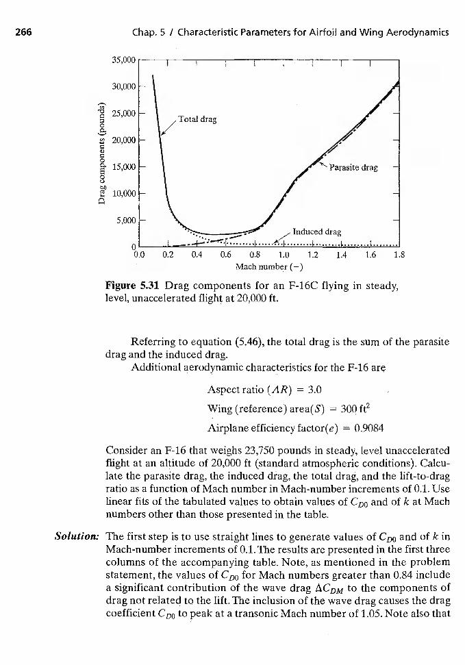
266 Chap. 5 / Characteristic Parameters for Airfoil and Wing Aerodynamics
C,,
C
C',
Q)
C
J
Figure 5.31 Drag components for an F-16Clevel, unaccelerated flight at 20,000 ft.
1.2 1.4 1.6 1.8
flying in steady,
Referring to equation (5.46), the total drag is the sum of the parasitedrag and the induced drag.
Additional aerodynamic characteristics for the F46
Aspect ratio (AR) = 3.0
Wing (reference) area(S) = 300 ft2
Airplane efficiency factor(e) = 0.9084
Consider an F-16 that weighs 23,750 pounds in steady, level unacceleratedflight at an altitude of 20,000 ft (standard atmospheric conditions). Calcu-late the parasite drag, the induced drag, the total drag, and the lift-to-dragratio as a function of Mach number in Mach-number increments of 0.1. Uselinear fits of the tabulated values to obtain values of CDO and of k at Machnumbers other than those presented in the table.
Solution: The first step is to use straight lines to generate values of CDO and of k inMach-number increments of 0.1.The results are presented in the first threecolumns of the accompanying table. Note, as mentioned in the problemstatement, the values of for Mach numbers greater 0.84 includea significant contribution of the wave drag to the components ofdrag not related to the lift. The inclusion of the wave drag causes the dragcoefficient CDO to peak at a transonic Mach number of 1.05. Note also that
o0.0 0.2 0.4 0.6 0.8 1.0
Mach number (—)
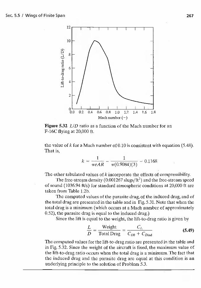
n
0
0
00.0 0.2 0.4 0.6 0.8 1.0 1.2 1.4
Mach number (—)
1 1k
= 7reAR == 0.1168
Sec. 5.5 I Wings of Finite Span 267
12
10
8
6
__
4
2
1.6 1.8
Figure 5.32 LID ratio as a function of the Mach number for anF-16C flying at 20,000 ft.
the value of k for a Mach number of 0.10 is consistent with equation (5.48).That is,
The other tabulated values of k incorporate the effects of compressibility.The free-stream density (0.001267 slugs/ft3) and the free-stream speed
of sound (1036.94 ft/s) for standard atmospheric conditions at 20,000 ft aretaken from Table 1.2b.
The computed values of the parasite drag, of the induced drag, and ofthe total drag are presented in the table and in Fig. 5.31. Note that when thetotal drag is a minimum (which occurs at a Mach number of approximately0.52), the parasite drag is equal to the induced drag.)
Since the lift is equal to the weight, the lift-to-drag ratio is given by
L — Weight — CL 549D — Total Drag — +
The computed values for the lift-to-drag ratio are presented in the table andin Fig. 5.32. Since the weight of the aircraft is fixed, the maximum value ofthe lift-to-drag ratio occurs when the total drag is a minimum. The fact thatthe induced drag and the parasite drag are equal at this condition is anunderlying principle to the solution of Problem 5.3.
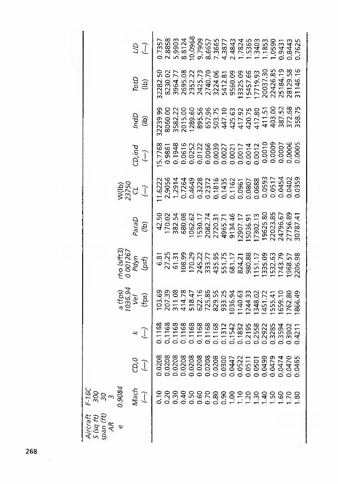
Airc
raft
F-1
6CS
(sq
ft)
300
span
(ft)
30A
R3
e0.
9084
a (f
ps)
1036
.94
rho
(s/ft
3)0.
0012
67W
(Ib)
2375
0M
ach
CD
,0k
Vel
Pdy
nP
araD
CL
CD
,ind
IndD
Tot
DLI
D
(—)
(—)
(—)
(fps
)(p
sf)
(Ib)
(—)
(—)
(Ib)
(Ib)
(—)
0.10
0.02
080.
1168
103.
696.
8142
.50
11.6
222
15.7
768
3223
9.99
3228
2.50
0.73
570.
200.
0208
0.11
6820
7.39
27.2
517
0.02
2.90
560.
9861
8060
.00
8230
.02
2.88
580.
300.
0208
0.11
6831
1.08
61.3
138
2.54
1.29
140.
1948
3582
.22
3964
.77
5.99
030.
400.
0208
0.11
6841
4.78
108.
9968
0.08
0.72
640.
0616
2015
.00
2695
.08
8.81
240.
500.
0208
0.11
6851
8.47
170.
2910
62.6
20.
4649
0.02
5212
89.6
023
52.2
210
.096
80.
600.
0208
0.11
6862
2.16
245.
2215
30.1
70.
3228
0.01
2289
5.56
2425
.73
9.79
090.
700.
0208
0.11
6872
5.86
333.
7720
82.7
40.
2372
0.00
6665
7.96
2740
.70
8.66
570.
800.
0208
0.11
6882
9.55
435.
9527
20.3
10.
1816
0.00
3950
3.75
3224
.06
7.36
650.
900.
0300
0.13
1293
3.25
551.
7549
65.7
10.
1435
0.00
2744
7.10
5412
.81
4.38
771.
000.
0447
0.15
4210
36.9
468
1.17
9134
.46
0.11
620.
0021
425.
6395
60.0
92.
4843
1.10
0.05
220.
1832
1140
.63
824.
2112
907.
170.
0961
0.00
1741
7.92
1332
5.09
1.78
241.
200.
0511
0.21
9512
44.3
398
0.88
1503
6.91
0.08
070.
0014
420.
7515
457.
661.
5365
1.30
0.05
010.
2558
1348
.02
1151
.17
1730
2.13
0.06
880.
0012
417.
8017
719.
931.
3403
1.40
0.04
900.
2922
1451
.72
1335
.09
1962
5.80
0.05
930.
0010
411.
5120
037.
301.
1853
1.50
0.04
790.
3285
1555
.41
1532
.63
2202
3.85
0.05
170.
0009
403.
0022
426.
851.
0590
1.60
0.04
740.
3594
1659
.10
1743
.79
2479
6.67
0.04
540.
0007
387.
5225
184.
190.
9431
1.70
0.04
700.
3902
1762
.80
2775
6.89
0.04
020.
0006
372.
6828
129.
580.
8443
1.80
0.04
650.
4211
1866
.49
2206
.98
3078
7.41
0.03
590.
0005
358.
7531
146.
160.
7625
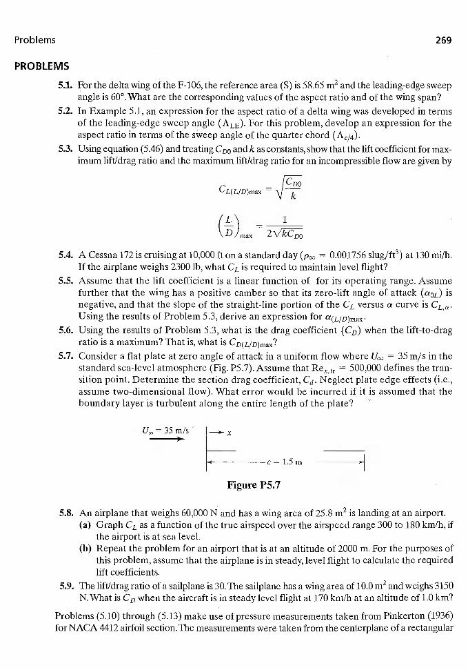
Problems 269
PROBLEMS
5.1. For the delta wing of the F-106, the reference area (S) is 58.65 m2 and the leading-edge sweepangle is 60°. What are the corresponding values of the aspect ratio and of the wing span?
5.2. In Example 5.1, an expression for the aspect ratio of a delta wing was developed in termsof the leading-edge sweep angle (ALE). For this problem, develop an expression for theaspect ratio in terms of the sweep angle of the quarter chord
5.3. Using equation (5.46) and treating CDO and k as constants, show that the lift coefficient for max-imum lift/drag ratio and the maximum lift/drag ratio for an incompressible flow are given by
CL(L/D)max=
—
5.4. A Cessna 172 is cruising at 10,000 ft on a standard day = 0.001756 slug/ft3) at 130 mi/h.If the airplane weighs 2300 lb, what CL is required to maintain level flight?
5.5. Assume that the lift coefficient is a linear function of for its operating range. Assumefurther that the wing has a positive camber so that its zero-lift angle of attack (aoL) isnegative, and that the slope of the straight-line portion of the CL versus a curve is CL,a.Using the results of Problem 5.3, derive an expression for
5.6. Using the results of Problem 5.3, what is the drag coefficient (CD) when the lift-to-dragratio is a maximum? That is, what is CD(L/D)max?
5.7. Consider a flat plate at zero angle of attack in a uniform flow where = 35 rn/s in thestandard sea-level atmosphere (Fig. P5.7).Assume that Rextr = 500,000 defines the tran-sition point. Determine the section drag coefficient, Cd. Neglect plate edge effects (i.e.,assume two-dimensional flow). What error would be incurred if it is assumed that theboundary layer is turbulent along the entire length of the plate?
= 35 rn/s
5.8. An airplane that weighs 60,000 N and has a wing area of 25.8 m2 is landing at an airport.(a) Graph CL as a function of the true airspeed over the airspeed range 300 to 180 km/h, if
the airport is at sea level.(b) Repeat the problem for an airport that is at an altitude of 2000 m. For the purposes of
this problem, assume that the airplane is in steady, level flight to calculate the requiredlift coefficients.
5.9. The lift/drag ratio of a sailplane is 30. The sailplane has a wing area of 10.0 m2 and weighs 3150N. What is CD when the aircraft is in steady level flight at 170 km/h at an altitude of 1.0 km?
Problems (5.10) through (5.13) make use of pressure measurements taken from Pinkerton (1936)for NACA 4412 airfoil section.The measurements were taken from the centerplane of a rectangular
x
Figure P5.7
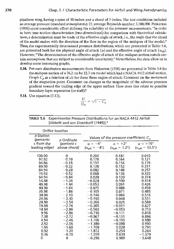
270 Chap. 5 I Characteristic Parameters for Airfoil and Wing Aerodynamics
planform wing, having a span of 30 inches and a chord of 5 inches. The test conditions includedan average pressure (standard atmospheres): 21; average Reynolds number: 3,100,000. Pinkerton(1936) spent considerable effort defining the reliability of the pressure measurements. "In orderto have true section characteristics (two-dimensional) for comparison with theoretical calcula-tions, a determination must be made of the effective angle of attack, i.e., the angle that the chordof the model makes with the direction of the flow in the region of the midspan of the model."Thus, the experimentally determined pressure distributions, which are presented in Table 5.6,are presented both for the physical angle of attack (a) and the effective angle of attackHowever, "The determination of the effective angle of attack of the midspan section entails cer-tain assumptions that are subject to considerable uncertainty?' Nevertheless, the data allow us todevelop some interesting graphs.5.10. Pressure distribution measurements from Pinkerton (1936) are presented in Table 5.6 for
the midspan section of a 76.2 cm by 12.7 cm model which had a NACA 4412 airfoil section.Graph as a function of x/c for these three angles of attack. Comment on the movementof the stagnation point. Comment on changes in the magnitude of the adverse pressuregradient toward the trailing edge of the upper surface. How does this relate to possibleboundary-layer separation (or stall)?
5.11. Use equation (3.13),
TABLE 5.6 Experimental Pressure Distributions for an NJACA 4412 Airfoil[Abbott and von Doenhoff
Orifice locationx-Station(percentc z-Ordinate
c from the (percent c
Values of the pressure coefficient, Ci,,
a = —4° a = +2° a = +16°leading edge) above chord) (cxeff = 4°) = 1.2°) (aeff = 13.5°)
100.00 0 0.204 0.181 0.01097.92 —0.10 0.178 0.164 0.12194.86 —0.16 0.151 0.154 0.17989.90 —0.22 0.128 0.152 0.23184.94 —0.28 0.082 0.148 0.25774.92 —0.52 0.068 0.136 0.32264.94 —0.84 0.028 0.120 0.37454.48 —1.24 —0.024 0.100 0.41449.98 —1.44 —0.053 0.091 0.42644.90 —1.64 —0.075 0.088 0.45939.98 —1.86 —0.105 0.071 0.48534.90 —2.10 —0.146 0.066 0.51629.96 —2.30 —0.190 0.048 0.55124.90 —2.54 —0.266 0.025 0.58919.98 —2.76 —0.365 —0.011 0.62714.94 —2.90 —0.502 —0.053 0.7139.96 —2.86 —0.716 —0.111 0.8187.38 —2.72 —0.867 —0.131 0.8964.94 —2.46 —1.106 —0.150 0.9802.92 —2.06 —1.380 —0.098 0.9931.66 —1.60 —1.709 0.028 0.7910.92 —1.20 —1.812 0.254 0.2640.36 —0.70 —1.559 0,639 —1.3790 0 —0.296 0.989 —3.648
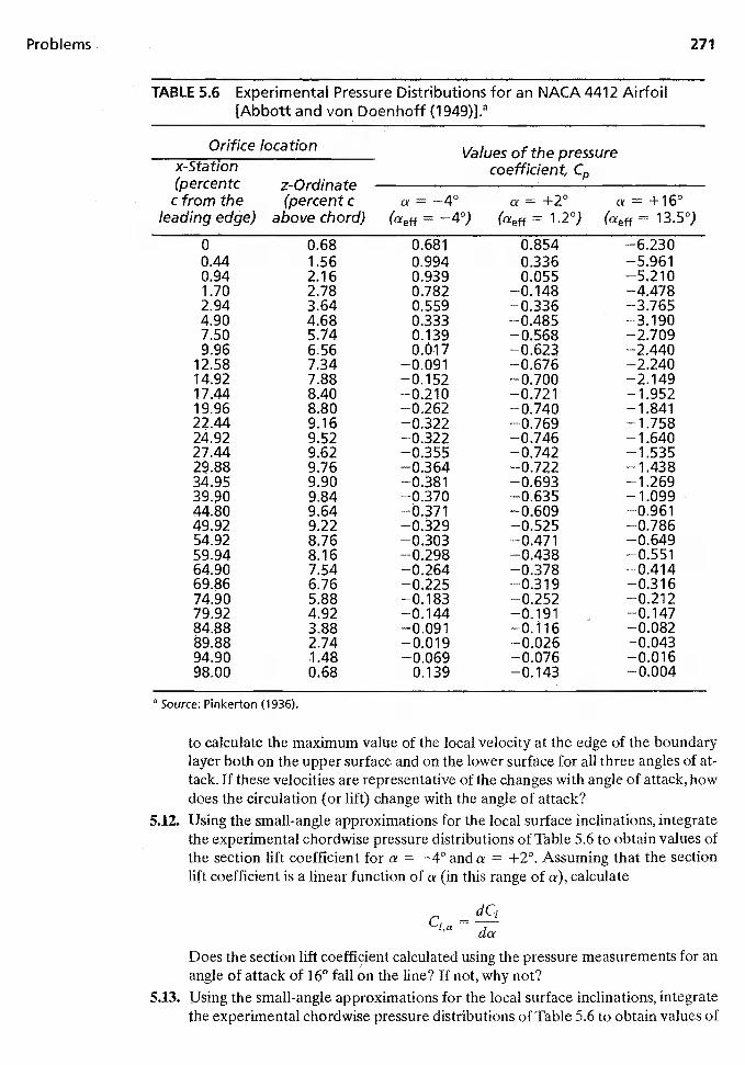
Problems 271
TABLE 5.6 Experimental Pressure Distributions for an NACA 4412 Airfoil[Abbott and von Doenhoff (1949)1.a
Orifice locationVa lues of the pressure
coeffident,x-Station('percentccfromthe
z-Ordinate(percentc a—4° a+2° a+16°
leading edge) above chord) (aeff 4°) (aeff = 1.2°) (aeff 13.50)
0 0.68 0.681 0.854 —6.2300.44 1.56 0.994 0.336 —5.9610.94 2.16 0.939 0.055 —5.2101.70 2.78 0.782 —0.148 —4.4782.94 3.64 0.559 —0.336 —3.7654.90 4.68 0.333 —0.485 —3.1907.509.96
5.746.56
0.1390.017
—0.568—0.623
—2.709—2.440
12.58 7.34 —0.091 —0.676 —2.24014.92 7.88 —0.152 —0.700 —2.14917.44 8.40 —0.210 —0.721 —1.95219.96 8.80 —0.262 —0.740 —1.84122.44 9.16 —0.322 —0.769 —1.75824.92 9.52 —0.322 —0.746 —1.64027.44 9.62 —0.355 —0.742 —1.53529.88 9.76 —0.364 —0.722 —1.43834.95 9.90 —0.381 —0.693 —1.26939.9044.80
9.849.64
—0.370—0.371
—0.635—0.609
—1.099—0.961
49.92 9.22 —-0.329 —0.525 —0.78654.92 8.76 —0.303 —0.471 —0.64959.94 8.16 —0.298 —0.438 —0.55164.90 7.54 —0.264 —0.378 —0.41469.86 6.76 —0.225 —0.319 —0.31674.90 5.88 —0.183 —0.252 —0.21279.92 4.92 —0.144 —0.191 —0.14784.88 3.88 —0.091 —0.116 —0.08289.88 2.74 —0.019 —0.026 —0.04394.90 1.48 —0.069 —0.076 —0.01698.00 0.68 0.139 —0.143 —0.004
Source: Pinkerton (1935).
to calculate the maximum value of the local velocity at the edge of the boundarylayer both on the upper surface and on the lower surface for all three angles of at-tack. If these velocities are representative of the changes with angle of attack, howdoes the circulation (or lift) change with the angle of attack?
5.12. Using the small-angle approximations for the local surface inclinations, integratethe experimental chordwise pressure distributions of Table 5.6 to obtain values ofthe section lift coefficient for a —4° and a = +2°. Assuming that the sectionlift coefficient is a linear function of a (in this range of a), calculate
dC1a = da
Does the section lift coefficient calculated using the pressure measurements for anangle of attack of 16° fall on the line? If not, why not?
5.13. Using the small-angle approximations for the local surface inclinations, integratethe experimental chordwise pressure distributions of Table 5.6 to obtain values of
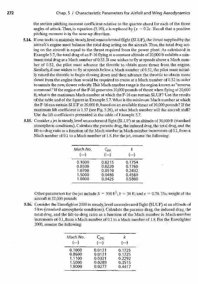
272 Chap. 5 / Characteristic Parameters for Airfoil and Wing Aerodynamics
the section pitching moment coefficient relative to the quarter chord for each of the threeangles of attack. Thus, in equation (5.10), x is replaced by (x — 0.2c. Recall that a positivepitching moment is in the nose-up direction.
5.14. If one seeks to maintain steady, level unaccelerated flight (SLUF), the thrust supplied by theaircraft's engine must balance the total drag acting on the aircraft. Thus, the total drag act-ing on the aircraft is equal to the thrust required from the power plant. As calculated inExample 5.7, the total drag of an F-16 flying at a constant altitude of 20,000 ft exhibits a min-imum total drag at a Mach number of 0.52. If one wishes to fly at speeds above a Mach num-ber of 0.52, the pilot must advance the throttle to obtain more thrust from the engine.Similarly, if one wishes to fly at speeds below a Mach number of 0.52, the pilot must initial-ly retard the throttle to begin slowing down and then advance the throttle to obtain morethrust from the engine than would be required to cruise at a Mach number of 0.52 in orderto sustain the new, slower This Mach number range is the region known as "reversecommand." If the engine of the F-16 generates 10,000 pounds of thrust when flying at 20,000ft, what is the maximum Mach number at which the F-i 6 can sustain SLUF? Use the resultsof the table and of the figures in Example 5.7.What is the minimum Mach number at whichthe F-i6 can sustain SLUF at 20,000 ft, based on an available thrust of 10,000 pounds? If themaximum lift coefficient is 1.57 (see Fig. 5.26), at what Mach number will the aircraft stall?Use the lift coefficients presented in the table of Example 5.7.
5.15. Consider a jet in steady, level unaccelerated flight (SLUF) at an altitude of 30,000 ft (standardatmospheric conditions). Calculate the parasite drag, the induced drag, the total drag, and thelift-to-drag ratio as a function of the Mach number in Mach-number increments of 0.1, from aMach number of 0.1 to a Mach number of 1.8. For the jet, assume the following:
Mach No.
(..—)
CDO
(—)
k
(—)
0.1000 0.0215 0.17540.8500 0.0220 0.1 7601.0700 0.0510 0.24321.5000 0.0486 0.45601.8000 0.042 5 0.5800
Other parameters for the jet include S = 500 ft2; b = 36 ft; and e = 0.70. The weight of theaircraft is 32,000 pounds.
5.16. Consider the Eurofighter 2000 in steady, level unaccelerated flight (SLUF) at an altitude of5 km (standard atmospheric conditions), Calculate the parasite drag, the induced drag, thetotal drag, and the lift-to-drag ratio as a function of the Mach number in Mach-numberincrements of 0.1, from a Mach number of 0.1 to a Mach number of 1.8. For the Eurofighter2000, assume the following:
Mach No.
(—)
C00
(—)
k(—)
0.1000 0.0131 0.17250.8600 0.0131 0.17251.1 100 0.0321 0.22921.5000 0.0289 0.35151.8000 0.0277 0.4417
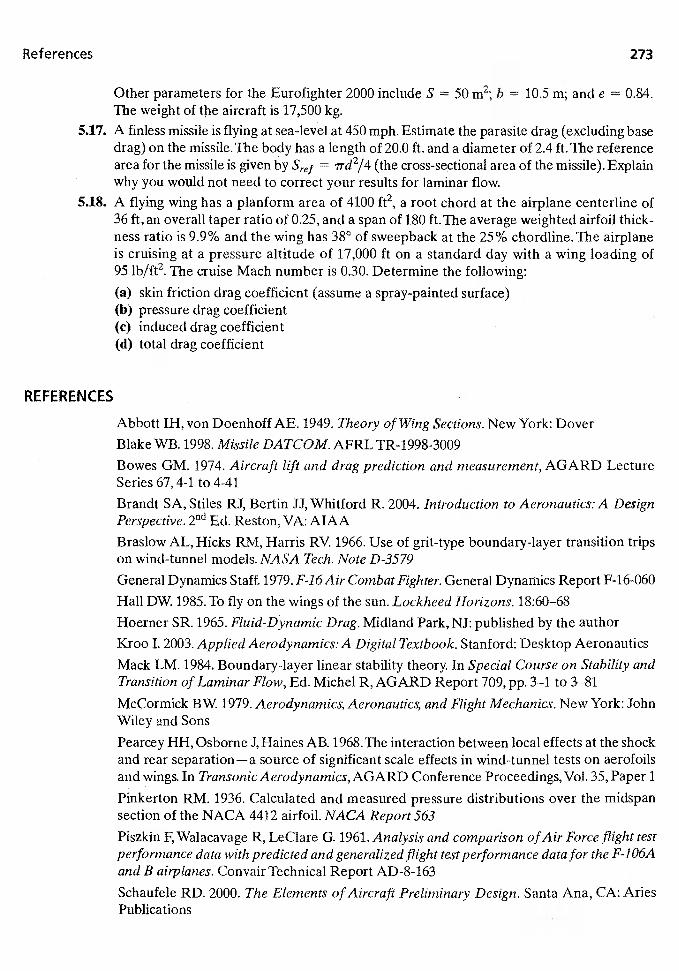
References 273
Other parameters for the Eurofighter 2000 include S = 50 m2; b = 10.5 m; and e = 0.84.The weight of the aircraft is 17,500 kg.
5.17. A finless missile is flying at sea-level at 450 mph. Estimate the parasite drag (excluding basedrag) on the missile.The body has a length of 20.0 ft. and a diameter of 2,4 ft.The referencearea for the missile is given by = lTd2/4 (the cross-sectional area of the missile). Explainwhy you would not need to correct your results for laminar flow.
5.18. A flying wing has a planform area of 4100 It2, a root chord at the airplane centerline of36 It, an overall taper ratio of 0.25, and a span of 180 ft.The average weighted airfoil thick-ness ratio is 9.9% and the wing has 38° of sweepback at the 25% chordline. The airplaneis cruising at a pressure altitude of 17,000 ft on a standard day with a wing loading of95 lb/ft2. The cruise Mach number is 0.30. Determine the following:
(a) skin friction drag coefficient (assume a spray-painted surface)(b) pressure drag coefficient(c) induced drag coefficient(d) total drag coefficient
REFERENCES
Abbott IH, von Doenhoff AE. 1949. Theory of Wing Sections. New York: Dover
Blake WB. 1998. Missile DATCOM. AFRL TR-1998-3009
Bowes GM. 1974. Aircraft lift and drag prediction and measurement, AGARD LectureSeries 67,4-ito 4-41Braridt SA, Stiles RJ, Bertin JJ, Whitford R. 2004. Introduction to Aeronautics: A DesignPerspective. 2nd Ed. Reston, VA: AIAA
Braslow AL, Hicks RM, Harris RV. 1966. Use of grit-type boundary-layer transition tripson wind-tunnel models. NASA Tech. Note D-3579
General Dynamics Staff. 1979. F-16 Air Combat Fighter. General Dynamics Report F-16-060
Hall DW. 1985. To fly on the wings of the sun. Lockheed Horizons. 18:60—68
Hoerner SR. 1965. Drag. Midland Park, NJ: published by the author
Kroo I. 2003. Applied Aerodynamics:A Digital Textbook. Stanford: Desktop Aeronautics
Mack LM. 1984. Boundary-layer linear stability theory. In Special Course on Stability andTransition of Laminar Flow, Ed. Michel R, AGARD Report 709, pp.3—i to 3—81
McCormick BW. 1979. Aerodynamics, Aeronautics, and Flight Mechanics. New York: JohnWiley and Sons
Pearcey HH, Osborne J, Haines AB. 1968. The interaction between local effects at the shockand rear separation—a source of significant scale effects in wind-tunnel tests on aerofoilsand wings. In Transonic Aerodynamics, AGARD Conference Proceedings, Vol. 35, Paper 1
Pinkerton RM. 1936. Calculated and measured pressure distributions over the midspansection of the NACA 4412 airfoil. NACA Report 563
Piszkin F,Walacavage R, LeClare G. 1961. Analysis and comparison ofAir Force flight testperformance data with predicted and generalized flight test performance data for the F-106Aand B airplanes. Convair Technical Report AD-8-163
Schaufele RD. 2000. The Elements of Aircraft Preliminary Design. Santa Ana, CA: AriesPublications
274 Chap. 5 / Characteristic Parameters for Airfoil and Wing Aerodynamics
Schlichting H. 1979. Boundary Layer Theory. 7th Ed. New York: McGraw-Hill
Shevell RS. 1989. Fundamentals of Flight. Ed. Englewood Cliffs, NJ: Prentice Hall
Sterret JR, Morrisette EL, Whitehead AH, Hicks RM. 1966. Transition fixing for hyper-sonic flow. NASA Tech. Note D-4129
Stuart WG. 1978. Northrop F-5 Case Study in Aircraft Design. Washington, DC: AIAA
Taylor JWR, ed. 1973. Jane's All the World's Aircraft, 1973—1974. London: Jane's Yearbooks
Taylor JWR, ed. 1966. Jane's All the World's Aircraft, 1966-1967. London: Jane's Yearbooks
Taylor JWR, ed. 1984. Jane's All the World'sAircraft, 1984—1985. London: Jane's Yearbooks
Thomas ASW. 1985. Aircraft viscous drag reduction technology, Lockheed Horizons19:22—32
Van Dam CP, Holmes BJ. 1986. Boundary-layer transition pifects on airplane stability andcontrol. Presented at Atmospheric Flight Mech. Couf., AIA4 Pap. 86-2229, Williamsburg,VA
Webb TS, Kent DR, Webb JB. 1977. Correlation of F-16 aerodynamics and performancepredictions with early flight test results. In Performance Prediction Methods, AGARDConference Proceeding, Vol. 242, 19
6 INCOMPRESSIBLE FLOWS
AROUND AIRFOILS OF
INFINITE SPAN
6.1 GENERAL COMMENTS
Theoretical relations that describe an inviscid, low-speed flow around a thin airfoil willbe developed in this chapter. To obtain the governing equations, it is assumed that theairfoil extends to infinity in both directions from the plane of symmetry (i.e., that the air-foil is a wing of infinite aspect ratio). Thus, the flow field around the airfoil is the samefor any cross section perpendicular to the wing span and the flow is two dimensional,
For the rest of this book, the term airfoil will be used when the flow field is twodimensional. Thus, it will used for the two-dimensional flow fields that would exist whenidentical airfoil sections are placed side by side so that the spanwise dimension of theresultant configuration is infinite. But the term airfoil will also be used when a finite-spanmodel with identical cross sections spans a wind tunnel from wall-to-wall and is per-pendicular to the free-stream flow. Neglecting interactions with the tunnel-wall bound-ary layer, the flow around the model does not vary in the spanwise direction. For manyapplications (see Chapter 7), these two-dimensional airfoil flow fields will be applied toa slice of a wing flow field. That is, they approximate the flow per unit width (or per unitspan) around the airfoil sections that are elements of a finite-span wing. For the rest ofthis book, the term wing will be used when the configuration is of finite span.
The flow around a two-dimensional airfoil can be idealized by superimposing a trans-lational flow past the airfoil section, a distortion of the stream that is due to the airfoilthickness, and a circulatory flow that is related to the lifting characteristics of the airfoil.
275
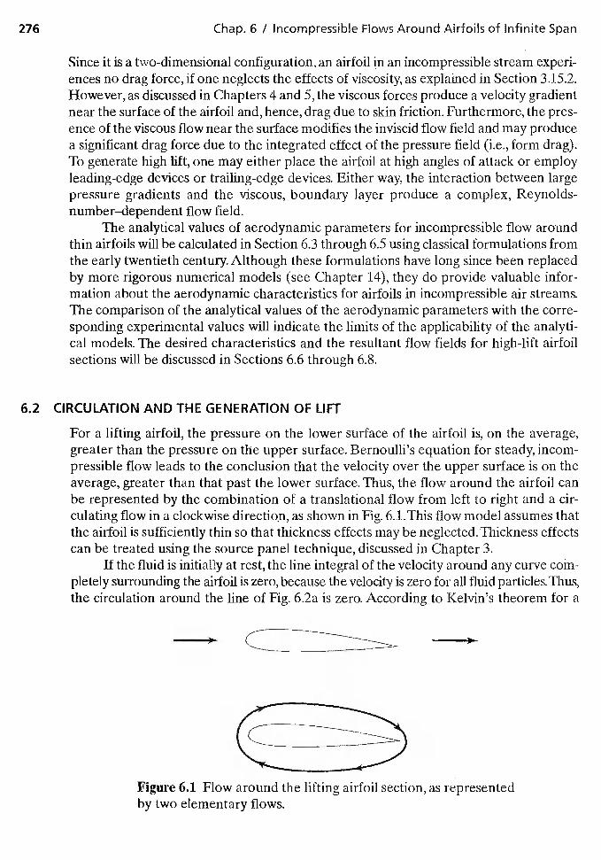
276 Chap. 6 / Incompressible Flows Around Airfoils of Infinite Span
Since it is a two-dimensional configuration, an airfoil jn an incompressible stream experi-ences no drag force, if one neglects the effects of viscosity, as explained in Section 3.15.2.However, as discussed in Chapters 4 and 5, the viscous forces produce a velocity gradientnear the surface of the airfoil and, hence, drag due to skin friction. Furthermore, the pres-ence of the viscous flow near the surface modifies the inviscid flow field and may producea significant drag force due to the integrated effect of the pressure field (i.e., form drag).To generate high lift, one may either place the airfoil at high angles of attack or employleading-edge devices or trailing-edge devices. Either way, the interaction between largepressure gradients and the viscous, boundary layer produce a complex, Reynolds-number—dependentflow field.
The analytical values of aerodynamic parameters for incompressible flow aroundthin airfoils will be calculated in Section 6,3 through 6.5 using classical formulations fromthe early twentieth century. Although these formulations have long since been replacedby more rigorous numerical models (see Chapter 14), they do provide valuable infor-mation about the aerodynamic characteristics for airfoils in incompressible air streams.The comparison of the analytical values of the aerodynamic parameters with the corre-sponding experimental values will indicate the limits of the applicability of the analyti-cal models. The desired characteristics and the resultant flow fields for high-lift airfoilsections will be discussed in Sections 6.6 through 6.8.
6.2 CIRCULATION AND THE GENERATION OF LIFT
For a lifting airfoil, the pressure on the lower surface of the airfoil is, on the average,greater than the pressure on the upper surface. Bernoulli's equation for steady, incom-pressible flow leads to the conclusion that the velocity over the upper surface is on theaverage, greater than that past the lower surface. Thus, the flow around the airfoil canbe represented by the combination of a translational flow from left to right and a cir-culating flow in a clockwise direction, as shown in Fig. 6.1.This flow model assumes thatthe airfoil is sufficiently thin so that thickness effects may be neglected.Thickness effectscan be treated using the source panel technique, discussed in Chapter 3.
If the fluid is initially at rest, the line integral of the velocity around any curve com-pletely surrounding the airfoil is zero, because the velocity is zero for all fluid particles. Thus,the circulation around the line of Fig. 6.2a is zero. According to Kelvin's theorem for a
Figure 6.1 Flow around the lifting airfoil section, as representedby two elementary flows.
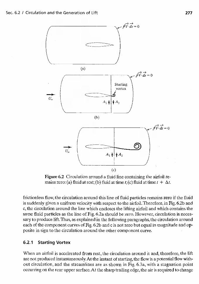
A1+$A2
(c)
Figure 6.2 Circulation around a fluid line containing the airfoil re-mains zero: (a) fluid at rest; (b) fluid at time t, (c) fluid at time t + t.
frictionless flow, the circulation around this line of fluid particles remains zero if the fluidis suddenly given a uniform velocity with respect to the airfoil. Therefore, in Fig. 6.2b andc, the circulation around the line which encloses the lifting airfoil and which contains thesame fluid particles as the line of Fig. 6.2a should be zero. However, circulation is neces-sary to produce lift. Thus, as explained in the following paragraphs, the circulation aroundeach of the component curves of Fig. 6.2b and c is not zero but equal in magnitude and op-posite in sign to the circulation around the other component curve.
6.2.1 Starting Vortex
When an airfoil is accelerated from rest, the circulation around it and, therefore, the liftare not produced instantaneously At the instant of starting, the flow is a potential flow with-out circulation, and the streamlines are as shown in Fig. 6.3a, with a stagnation pointoccurring on the rear upper surface. At the sharp trailing edge, the air is required to change
Sec. 6.2 I Circulation and the Generation of Lift 277
=0
(a)
Startingvortex
A14 tA2
(b)
fv. ds =0
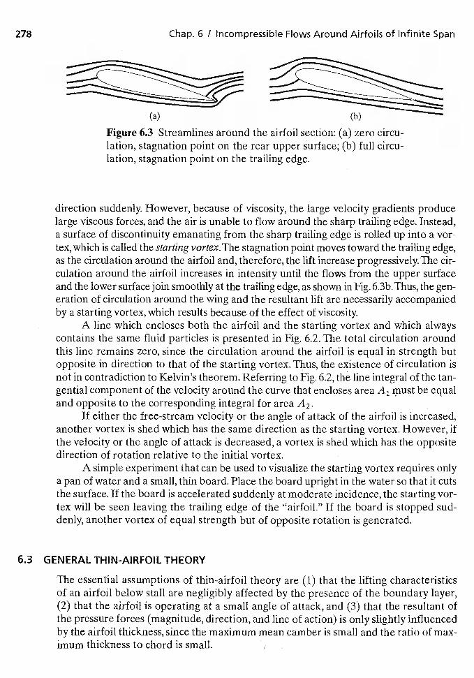
278 Chap. 6 I Incompressible Flows Around Airfoils of Infinite Span
(a) (b)
Figure 6,3 Streamlines around the airfoil section: (a) zero circu-lation, stagnation point on the rear upper surface; (b) full circu-lation, stagnation point on the trailing edge.
direction suddenly. However, because of viscosity, the large velocity gradients producelarge viscous forces, and the air is unable to flow around the sharp trailing edge. Instead,a surface of discontinuity emanating from the sharp trailing edge is rolled up into a vor-tex, which is called the starting vortex. The stagnation point moves toward the trailing edge,as the circulation around the airfoil and, therefore, the lift increase progressively. The cir-culation around the airfoil increases in intensity until the flows from the upper surfaceand the lower surface join smoothly at the trailing edge, as shown in Fig. 6.3b.Thus, the gen-eration of circulation around the wing and the resultant lift are necessarily accompaniedby a starting vortex, which results because of the effect of viscosity.
A line which encloses both the airfoil and the starting vortex and which alwayscontains the same fluid particles is presented in Fig. 6,2. The total circulation aroundthis line remains zero, since the circulation around the airfoil is equal in strength butopposite in direction to that of the starting vortex. Thus, the existence of circulation isnot in contradiction to Kelvin's theorem. Referring to Fig. 6.2, the line integral of the tan-gential component of the velocity around the curve that encloses area A1 must be equaland opposite to the corresponding integral for area A2.
If either the free-stream velocity or the angle of attack of the airfoil is increased,another vortex is shed which has the same direction as the starting vortex. However, ifthe velocity or the angle of attack is decreased, a vortex is shed which has the oppositedirection of rotation relative to the initial vortex.
A simple experiment that can be used to visualize the starting vortex requires onlya pan of water and a small, thin board. Place the board upright in the water so that it cutsthe surface, If the board is accelerated suddenly at moderate incidence, the starting vor-tex will be seen leaving the trailing edge of the "airfoil." If the board is stopped sud-denly, another vortex of equal strength but of opposite rotation is generated.
6.3 GENERAL THIN-AIRFOIL THEORY
The essential assumptions of thin-airfoil theory are (1) that the lifting characteristicsof an airfoil below stall are negligibly affected by the presence of the boundary layer,(2) that the airfoil is operating at a small angle of attack, and (3) that the resultant ofthe pressure forces (magnitude, direction, and line of action) is only slightly influencedby the airfoil thickness, since the maximum mean camber is small and the ratio of max-imum thickness to chord is small.
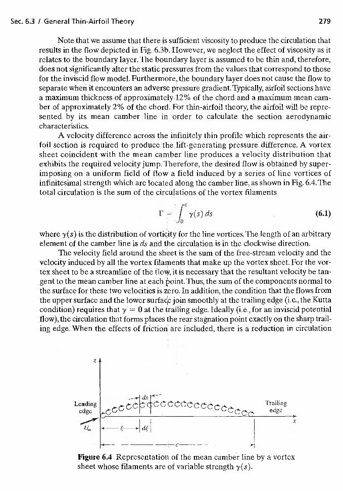
Sec. 6.3 / General Thin-Airfoil Theory 279
Note that we assume that there is sufficient viscosity to produce the circulation thatresults in the flow depicted in Fig. 6.3b. However, we neglect the effect of viscosity as itrelates to the boundary layer. The boundary layer is assumed to be thin and, therefore,does not significantly alter the static pressures from the values that correspond to thosefor the inviscid flow model. Furthermore, the boundary layer does not cause the flow toseparate when it encounters an adverse pressure gradient. Typically, airfoil sections havea maximum thickness of apprOximately. 12% of the chord and a maximum mean cam-ber of approximately 2% of the chord. For thin-airfoil theory, the airfoil will be repre-sented by its mean camber line in order to calculate the section aerodynamiccharacteristics.
A velocity difference across the infinitely thin profile which represents the air-foil section is required to produce the lift-generating pressure difference. A vortexsheet coincident with the mean camber line produces a velocity distribution thatexhibits the required velocity jump. Therefore, the desired flow is obtained by super-imposing on a uniform field of flow a field induced by a series of line vortices ofinfinitesimal strength which are located along the camber line, as shown in Fig. 6.4. Thetotal circulation is the sum of the circulations of the vortex filaments
F.= / y(s)ds (6.1)JO
where y(s) is the distribution of vortiqity for the line vortices. The length of an arbitraryelement of the camber line is ds and the circulation is in the clockwise direction.
The velocity field around the sheet is the sum of the free-stream velocity and thevelocity induced by all the vortex filaments that make up the vortex sheet. For the vor-tex sheet to be a streamline of the flow, it is necessary that the resultant velocity be tan-gent to the mean camber line at each point. Thus, the sum of the components normal tothe surface for these two velocities is zero. In addition, the condition that the flows fromthe upper surface and the lower join smoothly at the trailing edge (i.e., the Kuttacondition) requires that 'y 0 at the trailing edge. Ideally for an inviscid potentialflow), the circulation that forms places the rear stagnation point exactly on the sharp trail-ing edge. When the effects of friction are included, there is a reduction in circulation
Leadingedge
Figure 6.4 Representation of the mean camber line by a vortexsheet whose filaments are of variable strength 'y(s).
z
Trailing
x
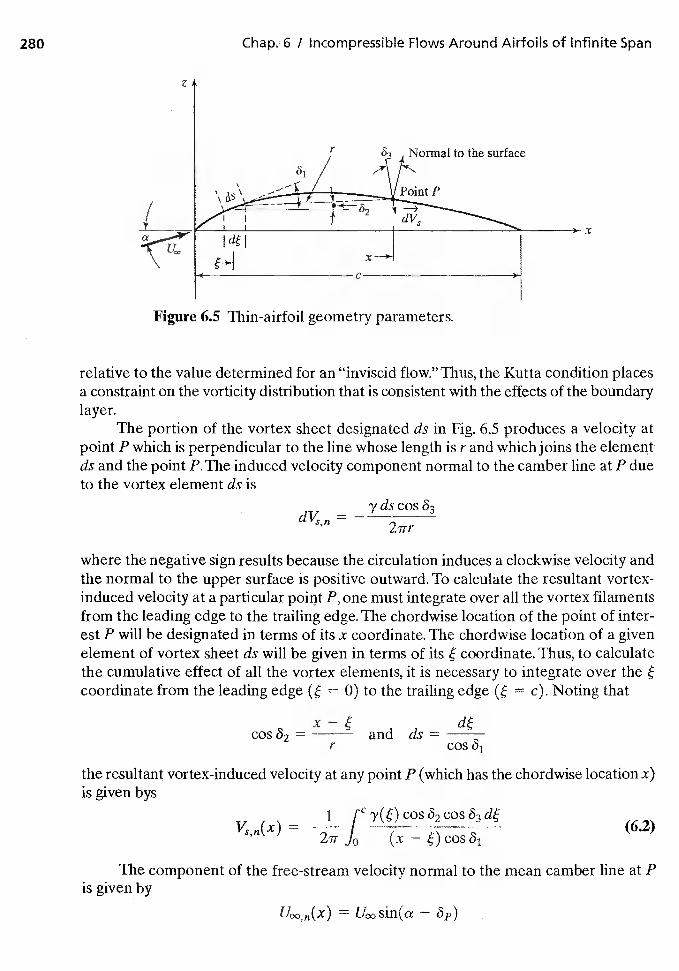
280 6 I Incompressible Flows Around Airfoils of Infinite Span
x
relative to the value determined for an "inviscid flow." Thus, the Kutta condition placesa constraint on the vorticity distribution that is consistent with the effects of the boundarylayer.
The portion of the vortex sheet designated ds in Fig. 6.5 produces a velocity atpoint P which is perpendicular to the line whose length is r and which joins the elementds and the point P.The induced velocity component normal to the camber line at P dueto the vortex element ds is
uvsn2'rr
where the negative sign results because the circulation induces a clockwise velocity andthe normal to the upper surface is positive outward. To calculate the resultant vortex-induced velocity at a particular point P, one must integrate over all the vortex filamentsfrom the leading edge to the trailing edge. The chordwise location of the point of inter-est P will be designated in terms of its x coordinate. The chordwise location of a givenelement of vortex sheet ds will be given in terms of its coordinate. Thus, to calculatethe cumulative effect of all the vortex elements, it is necessary to integrate over thecoordinate from the leading edge = 0) to the trailing edge = c). Noting that
cosf52 = and dsr cos61
the resultant vortex-induced velocity at any point P (which has the chordwise location x)is given bys
1= —---— I (6.2)
The component of the free-stream velocity normal to the mean camber line at Pis given by
= — 8p)
z
Normal to the surface
Figure 6.5 Thin-airfoil geometry parameters.
Sec. 6.4 I Thin, Flat-Plate Airfoil (Symmetric Airfoil) 281
where a is the angle of attack and Op is the slope of the camber line at the point of in-terest P. Thus,
dz—j—ax
where z(x) describes the mean camber line. As a result,
uco sin(a — tan1 (6.3)
Since the sum of the velocity components normal to the surface must be zero atall points along the vortex sheet,
1 cos 02 COS 03 /1
dz'\I = sin! a — J (6.4)
2ir j0 (x — dxj
The vorticity distribution that satisfies this integral equation makes the vortexsheet (and, therefore, the mean camber line) a streamline of the flow. The desired vor-ticity distribution must also satisfy the Kutta condition that y(c) 0.
Within the assumptions of thin-airfoil theory, the angles 82, 03, and a are small.Using the approximate trigonometric relations for small angles, equation (6.4) becomes
1 ( dz\I (6.5)
\. dxi
6.4 THIN, FLAT-PLATE AIRFOIL (SYMMETRIC AIRFOIL)
The mean camber line of a symmetric airfoil is coincident with the chord line. Thus,when the profile is replaced by its mean camber line, a flat plate with a sharp leadingedge is obtained. For subsonic flow past a flat plate even at small angles of attack, aregion of dead air (or stalled flow) will exist over the upper surface. For the actualairfoil, the rounded nose allows the flow to accelerate from the stagnation point ontothe upper surface without separation. Of course, when the angle of attack is suffi-ciently large (the value depends on the cross-section geometry), stall will occur forthe actual profile. The approximate theoretical solution for a thin airfoil with twosharp edges represents an irrotational flow with finite velocity at the trailing edge butwith infinite velocity at the leading edge. Because it does not account for the thicknessdistribution nor for the viscous effects, the approximate solution does not describethe chordwise variation of the flow around the actual airfoil. However, as will be dis-cussed, the theoretical values of the lift coefficient (obtained by integrating the cir-culation distribution along the airfoil) are in reasonable agreement with theexperimental values.
For the camber line of the symmetric airfoil, dzidx is everywhere zero. Thus, equa-tion (6.5) becomes
fc= (6.6)
282 Chap. 6 / Incompressible Flows Around Airfoils of Infinite Span
It is convenient to introduce the coordinate transformation
= — cos0) (6.7)
Similarly, the x coordinate transforms to 0o using
x = — cos0o)
The corresponding limits of integration are
and
Equation (6.6) becomesi y(0)sin0d0
I = (6.8)21Tj0 cos0—cos00
The required vorticity distribution, y(O), must not only satisfy this integral equation,but must satisfy the Kutta condition, y(ir) = 0. The solution is
1 + cos 0'y(O) = . (6.9)
sin 0
That this is a valid solution can be seen by substituting the expression for 'y(O) given byequation (6.9) into equation (6.8). The resulting equation,
'IT j0 cos0—cosO0
can be reduced to an identity using the relation
nO dO = sin nO0(6.10)
Jo COS 0 — COS sin 0o
where n assumes only integer values. Using l'Hospital's rule, it can be readily shownthat the expression for 'y(O) also satisfies the Kutta condition.
The Kutta-Joukowski theorem for steady flow about a two-dimensional body ofany cross section shows that the force per unit span is equal to and acts per-pendicular to Thus, for two-dimensional inviscid flow, an airfoil has no drag but ex-periences a lift per unit span equal to the product of free-stream density, the free-streamvelocity, and the total circulation. The lift per unit span is
= J(6.11)
0
Using the circulation distribution of equation (6.9) and the coordinate transformationof equation (6.7), the lift per unit span is
=
f (1 + cos 0) dO
— ( . )
Sec. 6.4 / Thin, Flat-Plate Airfoil (Symmetric Airfoil) 283
To determine the section lift coefficient of the airfoil, note that the reference area perunit span is the chord. The section lift coefficient is
C1 = 22'ira (6.13)
where a is the angle of attack in radians. Thus, thin-airfoil theory yields a section liftcoefficient for a symmetric airfoil that is directly proportional to the geometric angle ofattack.The geometric angle of attack is the angle between the free-stream velocity and thechord line of the airfoil. The theoretical relation is independent of the airfoil thickness.
However, because the airfoil thickness distribution and the boundary layer affectthe flow field, the actual two-dimensional lift curve slope will be less than 2ir per radian.See the discussion in Section 5.4.1.
It may seem strange that the net force for an inviscid flow past a symmetric airfoilis perpendicular to the free-stream flow rather than perpendicular to the airfoil (i.e.,that the resultant force has only a lift component and not both a lift and a drag compo-nent). As noted in Section 3.15.2, the prediction of zero drag may be generalized to anygeneral, two-dimensional body in an irrotational, steady, incompressible flow. Consideran incompressible, inviscid flow about a symmetric airfoil at a small angle of attack.There is a stagnation point on the lower surface of the airfoil just downstream of the lead-ing edge. From this stagnation point, flow accelerates around the leading edge to theupper surface. Referring to the first paragraph in this section, the approximate theoret-ical solution for a thin, symmetric airfoil with two sharp edges yields an infinite veloci-ty at the leading edge. The high velocities for flow over the leading edge result in lowpressures in this region, producing a component of force along the leading edge, knownas the leading-edge suction force, which exactly cancels the streamwise component of thepressure distribution acting on the rest of the airfoil, resulting in zero drag.
As noted by Carison and Mack (1980), "Linearized theory places no bounds on themagnitude of the peak suction pressure, which, therefore, can become much greaterthan practically realizable values." However, "limitations imposed by practically realiz-able pressures may have a relatively insignificant effect on the normal force but could,at the same time, severely limit the attainment of the thrust force."
The pressure distribution also produces a pitching moment about the leading edge(per unit span), which is given by
=— J
(6.14)0
The lift-generating circulation of an element produces an upward force that acts a dis-tance downstream of the leading edge. The lift force, therefore, produces a nose-downpitching moment about the leading edge. Thus, the negative sign is used in equation(6.14) because nose-up pitching moments are considered positive. Again, using the co-ordinate transformation [equation (6.7)] and the circulation distribution [equation (6.9)],the pitching moment (per unit span) about the leading edge is
m0 = f (1 — cos2 0) dO
— (6.15)
284 Chap. 6 / Flows Around Airfoils of Infinite Span
The section moment coefficient is given by
= m02
(6.16)°
Note that the reference area per unit span for the airfoil is the chord and the referencelength for the pitching moment is the chord. For the symmetric airfoil,
Cl= — — (6.17)
The center of pressure is the x coordinate, where the resultant lift force couldbe placed to produce the pitching moment m0. Equating the moment about the lead-ing edge [equation (6.15)] to the product of the lift [equation (6.12)] and the center ofpressure yields
2 2 2— =
Solving for xq,, one obtains
= (6.18)
The result is independent of the angle of attack and is therefore independent of the sec-tion lift coefficient.
EXAMPLE 6.1: Theoretical aerodynamic coefficients for a symmetricairfoil
The theoretical aerodynamic coefficients calculated using the thin-airfoil re-lations are compared with the data of Abbottand von Doenhoff (1949) inFig. 6.6. Data are presented for two different airfoil sections. One, the NACA0009, has a maximum thickness which is 9% of chord and is located atx = 0.3c. The theoretical lift coefficient calculated using equation (6.13) is inexcellent agreement with the data for the NACA 0009 airfoil up to an angleof attack of 12°. At higher angles of attack, the viscous effects significantlyalter the flow field and hence the experimental lift coefficients. Thus, theo-retical values would not be expected to agree with the data at high angles ofattack. Since the theory presumes that viscous effects are small, it is valid onlyfor angles of attack below stall. According to thin-airfoil theory, the momentabout the quarter chord is zero. The measured moments for the NACA 0009are also in excellent agreement with theory prior to stall. The correlation be-tween the theoretical values and the experimental values is not as good for theNACA 0012—64 airfoil section. The difference in the correlation between the-ory and data for these two airfoil sections is attributed to viscous effects. Themaximum thickness of the NACA 0012—64 is greater and located farther aft.Thus, the adverse pressure gradients that cause separation of the viscousboundary layer and thereby alter the flow field would be greater for theNACA 0012—64.
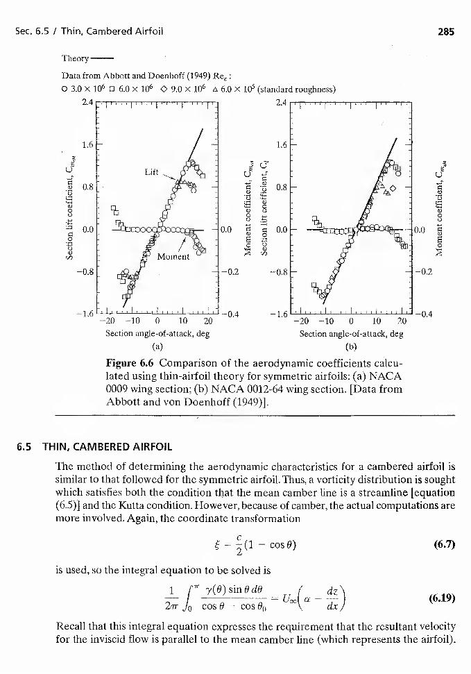
Sec. 6.5 I Thin, Cambered Airfoil
Theory
Data from Abbott and Doenhoff (1949) Ret:0 3.0 X 10⁶ 0 6.0 x 10⁶ 9.0 X 10⁶ 6.0 X (standard roughness)
2.4 11t!.JiI11r1I,.. 2.4
1.6- 1.6
Lift
a.) 08— —
0,0-0
a)
—0.8—
285
C
a)a)
a)0a)
0.8
L
a)0
o °a)
0.0 0.0
—0.2 —0.8
0.0
—0.2
—20 —10 0 10 20
Section angle-of-attack, deg
—0.4 —1.6
(a)
—20 —10 0 10 20
Section angle-of-attack, deg
—0.4
(b)
Figure 6.6 Comparison of the aerodynamic coefficients calcu-lated using thin-airfoil theory for symmetric airfoils: (a) NACA0009 wing section; (b) NACA 0012-64 wing section. [Data fromAbbott and von Doenhoff (1949)J.
6.5 THIN, CAMBERED AIRFOIL
The method of determining the aerodynamic characteristics for a cambered airfoil issimilar to that followed for the symmetric airfoil. Thus, a vorticity distribution is soughtwhich satisfies both the condition that the mean camber line is a streamline [equation(6.5)1 and the Kutta condition. However, because of camber, the actual computations aremore involved. Again, the coordinate transformation
= — cosO) (6.7)
is used, so the integral equation to be solved is
if1Ty(O)sinOdO
—
(6.19)2ir cosO — cosO0 dx
Recall that this integral equation expresses the requirement that the resultant velocityfor the inviscid flow is parallel to the mean camber line (which represents the airfoil).
286 Chap. 6 / Incompressible Flows Around Airfoils of Infinite Span
The vorticity distribution y(0) that satisfies the integral equation makes the vortex sheet(which is coincident with the mean camber line) a streamline of the flow.
6.51 Vorticity Distribution
The desired vorticity distribution, which satisfies equation (6.19) and the Kutta condi-tion, may be represented by the series involving
1. A term of the form for the vorticity distribution for a symmetric airfoil,
1 + cos82UcoA0
srn 8
2. A Fourier sine series whose terms automatically satisfy the Kutta condition,
The coefficients of the Fourier series depend on the shape of the camber line.Thus,
7(0) = + (6.20)sin0 n=1
Since each term is zero when B = the Kutta condition is satisfied [i.e., = 01.
Substituting the vorticity distribution [equation (6.20)1 into equation (6.19) yields
1 A0(1 + cos0) dO + j. = —(6.21)
Jo cosO — cosO0 ir Jo cos8 cos00 dx
This integral equation can be used to evaluate the coefficients A0, A1, A2, ... , interms of the angle of attack and the mean camber-line slope, which is known for a givenairfoil section. The first integral on the side of equation (6.21) can be readilyevaluated using equation (6.10). To evaluate the series of integrals represented by thesecond term, one must use equation (6.10) and the trigonometric identity:
(sinn0)(sin0) = 0.5[cos(n — 1)0 — cos(n + 1)8]
Equation (6.21) becomes
= a — A0 + cos nO (6.22)
which applies to any chordwise station. Since we are evaluating both dz/dx and cos nO0at the general point (i.e.,x), we have dropped the subscript 0 from equation (6.22) andfrom all subsequent equations. Thus, the coefficients A0, A1, A2,. .., must satisfyequation (6.22) if equation (6.20) is to represent the vorticity distribution which satis-fies the condition that the mean camber line is a streamline. Since the geometry of themean camber line would be known for the airfoil of interest, the slope is a known func-tion of 0. One can, therefore, determine the values of the coefficients.
Sec. 6.5 / Thin) Cambered Airfoil 287
To evaluate A0, note thatfir
/JO
thr any value of n. Thus, by algebraic manipulation of equation (6.22),
'.ir1 j dz
A0 a — j — dOdx
Multiplying both sides of equation (6.22) by cos mO, where m is an unspecified integer,and integratihg frdni 0 to ir, one obtains
IT IT ITOO
f cos mO dO / (a — A0) cos mO dO + / A,, cos nO cos mO dOJO X .10 JO
The first term on the right-hand side is zero for any value of m. Note that
P1T
/ A,, cos nO cos mU dO 0 when n inJO
butfir
/ A,, cos nO cos mU dO TA,, when n m2
Thus,2fdz
A,, — j — cos nO dO (6.24)1Tj0 dx
Using equations (6.23) and (6.24) to define the coefficients, equation (6.20) can be usedto evaluate the vorticity distribution for a cambered airfoil in terms of the geometricangle of attack and the shape of the mean line. Note that, for a symmetric air-foil, A0 = a, A1 = A2 = A,, = 0. Thus, the vorticity distribution for a symmetricairfOil, as determined using equation (6.20), is
1 + cos 0y(O) =
This is identical to equation (6.9). Therefore, the general expression for the camberedairfoil includes the symmetric airfoil as a special case.
6.S.2 Aerodynamic Coefficients for a Cambered Airfoil
The lift and the moment coefficients for a cambered airfoil are found in the same manneras for the symmetric airfoil. The section lift coefficient is given by
1=- 2 I
Jo
Using the coordinate transformation [equation (6.7)] and the expression for y [equation(6,20)] gives us
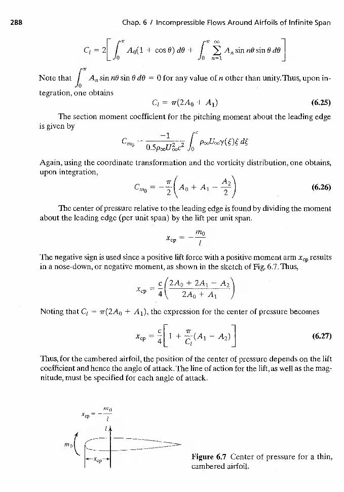
288 Chap. 6 / Incompressible Flows Around Airfoils of Infinite Span
C1 = 21] A0( 1 + cos 0) dO+ J
sin nO sin 0 dOL 0 0 n1
'IT
Note that I sin nO sin 0 dO = 0 for any value of n other than unity. Thus, upon in-Jo
tegration, one obtainsC1 = + A1) (6.25)
The section moment coefficient for the pitching moment about the leading edgeis given by
-1C,fl0
2 2 /Jo
Again, using the coordinate transformation and the vorticity distribution, one obtains,upon integration,
Cm0 = — + A1—
(6.26)
The center of pressure relative to the leading edge is found by dividing the momentabout the leading edge (per unit span) by the lift per unit span.
'noxcp
The negative sign is used since a positive lift force with a positive moment arm resultsin a nose-down, or negative moment, as shown in the sketch of Fig. 6.7. Thus,
cf2Ao + 2A1 A2
2A0+A1
Noting that C1 = ?r(2A0 + A1), the expression for the center of pressure becomes
= + — A2)] (6.27)
Thus, for the cambered airfoil, the position of the center of pressure depends on the liftcoefficient and hence the angle of attack, The line of action for the lift, as well as the mag-nitude, must be specified for each angle of attack.
xcp = —
mo(
Figure 6.7 Center of pressure for a thin,cambered airfoil.
Sec. 6.5 / Thin, Cambered Airfoil 289
If the pitching moment per unit span produced by the pressure distribution isreferred to a point O.25c downstream of the leading edge (i.e., the quarter chord), themoment is given by
O.25c c
= f - - -Again, the signs are chosen so that a nose-up moment is positive. Rearranging the rela-tion yields
pC
= £ j — J0
The first integral on the right-hand side of this equation represents the lift per unit span,while the second integral represents the moment per unit span about the leading edge. Thus,
mo2SC = + rn0 (6.28)
The section moment coefficient about the quarter-chord point is given by
Cm025 = + Cm0 (A2 — A1) (6.29)
Since A1 and A2 depend on the camber only, the section moment coefficient about thequarter-chord point is independent of the angle of attack. The point about which the sec-tion moment coefficient is independent of the angle of attack is called the aerodynamiccenter of the section. Thus, according to the theoretical relations for a thin-airfoil section,the aerodynamic center is at the quarter-chord point.
In order for the section pitching moment to remain constant as the angle of attackis increased, the product of the moment arm (relative to the aerodynamic center) andC1 must remain constant.Thus, the moment arm (relative to the aerodynamic center) de-creases as the lift increases. This is evident in the expression for the center of pressure,which is given in equation (6.27). Alternatively, the aerodynamic center is the point atwhich all changes in lift effectively take place. Because of these factors, the center ofgravity is usually located near the aerodynamic center. If we include the effects of vis-cosity on the flow around the airfoil, the lift due to angle of attack would not necessar-ily be concentrated at the exact quarter-chord point. However, for angles of attack belowthe onset of stall, the actual location of the aerodynamic center for the various sectionsis usually between the 23% chord point and the 27% chord point.Thus, the moment co-efficient about the aerodynamic center, which is given the symbol is also given byequation (6.29). If equation (6.24) is used to define A1 and A2, then becomes
Cm = (cos 20 cos 0) dO (6.30)ac 2 dX
Note, as discussed when comparing theory with data in the preceding section, the Cmacis zero for symmetric airfoil.
290 Chap. 6 / Incompressible Flows Around Airfoils of Infinite Span
EXAMPLE 62 Theoretical aerodynamic coefficients for a cambered airfoil
The relations developed in this section will nOw be used to calculate the aero-dynamic coefficients for a representative airfoil section. The airfoil sectionselected for use in this sample problem is the NACA 2412. As discussed in Ab-bott and Doenhoff (1949) the first digit defines the maximum camber in per-cent of chord, the second digit defines the location of the maximum camberin tenths of chord, and the last two digits represent the thickness ratio (i.e., themaximum thickness in percent of chord). The equation for the mean camberline is defined in terms of the maximum camber and its location. Forward ofthe maxtmum camber position, the equation of the mean camber line is
=—
C fore L C C
while aft of the maximum camber position,
= 0.0555[0.2 + 0.8(i) —
Solution: To calculate the section lift coefficient and the section moment coefficient,it is necessary to evaluate the coefficients A0, A1, and A2. To evaluate thesecoefficients it is necessary to integrate an expression involving the functionwhich defines the slope of the mean camber line. Therefore, the slope of themean camber line will be expressed in terms of the 8 coordinate, which isgiven in equation (6.7). Forward of the maximum camber location, the slopeis given by
0.1 — = 0.125 cos 8 — 0.025\dXJfore C
Aft of the maximum camber location, the slope is given by
(—n 0.0444 — = 0.0555cos0 — 0.0111c
Since the maximum camber location serves as a limit for the integrals, it isnecessary to convert the x coordinate, which is 0.4ç, to the corresponding 0coordinate. To do this,
— cos8) = 0.4c
Thus, the location of the maximum camber is 0 = 78.463° = 1.3694 rad.Referring to equations (6.23) and (6.24), the necessary coefficients are
1 r pl.3694A0 = a — / (0.125 cos 0 — 0.025) dO + / (0.0555 cos 0 0.0111) dO
.11.3694
a — 0.004517
Sec. 6.5 / Thin, Cambered Airfoil 291
2 1 c'-3694A1 = —I I (0.125cos28 — 0.O2ScosO)dO
L Jo
+ f (0.0555cos29 — 0.0111 cosO) do]13694
= 0.08146
2A2 = —I I (0.l2ScosOcos2O — 0.025 cos 20) dO
L JopIT
+ (0.OS5ScosOcos2O — 0.0111 cos2O) dO113694
= 0.01387
The section lift coefficient is
C1 = 2ir A0 + = 2ira + 0,2297
Solving for the angle of attack for zero lift, we obtain
= — 0.2297rad = —2.095°
2ir
According to thin-airfoil theory, the aerodynamic center is at the quar-ter-chord point. Thus, the section moment coefficient for the moment aboutthe quarter chord is equal to that about the aerodynamic center. The two co-efficients are given by
Cm = = —A1) = —0.05309
The theoretical values of the section lift coefficient and of the section moment co-efficients are compared with the measured values from Abbott and Doenhoff (1949) inFigs. 6.8 and 6.9, respectively. Since the theoretical coefficients do not depend on theairfoil section thickness, they will be compared with data from Abbott and Doenhoff(1949) for a NACA 2418 airfoil as well as for a NACA 2412 airfoil. For both airfoil sec-tions, the maximum camber is 2% of the chord length and is located at x = 0.4c. Themaximum thickness is 12% of chord for the NACA 2412 airfoil section and is 18% ofthe chord for the NACA 2418 airfoil section.
The correlation between the theoretical and the experimental values of lift is sat-isfactory for both airfoils (Fig. 6.8) until the angle of attack becomes so large that vis-cous phenomena significantly affect the flow field. The theoretical value for the zero liftangle of attack agrees very well with the measured values for the two airfoils. The the-oretical value of Cj,a is 217- per radian. Based on the measured lift coefficients for anglesof attack for 0° to 10°, the experimental value of Cia is approximately 6.0 per radian forthe NACA 2412 airfoil and approximately 5.9 per radian for the NACA 2418 airfoil.
The experimental values of the moment coefficient referred to the aerodynamiccenter (approximately —0.045 for the NACA 2412 section and —0.050 for the NACA
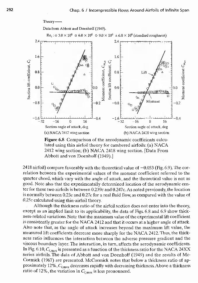
—16 0 16
Section angle of attack, deg
(a) NACA 2412 wing section
Figure 6.8 Comparison of the aerodynamic coefficients calcu-lated using thin airfoil theory for cambered airfoils: (a) NACA2412 wing section; (b) NACA 2418 wing section. [Data FromAbbott and von Doenhoff (1949).]
2418 airfoil) compare favorably with the theoretical value of —0.053 (Fig. 6.9). The cor-relation between the experimental values of the moment coefficient referred to thequarter chord, which vary with the angle of attack, and the theoretical value is not asgood. Note also that the experimentally determined location of the aerodynamic cen-ter for these two airfoils is between 0.239c and 0,247c. As noted previously, the locationis normally between 0.23c and 0.27c for a real fluid flow, as compared with the value ofO.25c calculated using thin-airfoil theory.
Although the thickness ratio of the airfoil section does not enter into the theory,except as an implied limit to its applicability, the data of Figs. 6.8 and 6.9 show thick-ness-related variations. Note that the maximum value of the experimental lift coefficientis consistently greater for the NACA 2412 and that it occurs at a higher angle of attack.Also note that, as the angle of attack increases beyond the maximum lift value, themeasured lift coefficients decrease more sharply for the NACA 2412. Thus, the thick-ness ratio influences the interaction between the adverse pressure gradient and theviscous boundary layer. The interaction, in turn, affects the aerodynamic coefficients.In Fig. 6.10, C1 max is presented as a function of the thickness ratio for the NACA 24XXseries airfoils. The data of Abbott and von Doenhoff (1949) and the results of Mc-Cormick (1967) are presented. McCormick notes that below a thickness ratio of ap-proximately 12%, Ci,max decreases rapidly with decreasing thickness. Above a thicknessratio of 12%, the variation in C1 max is less pronounced.
0
a)0U
0Ua)
292 Chap. 6 / Incompressible Flows Around Airfoils of Infinite Span
Theory—
Data from Abbott and Doenhoff (1949).
: o 3.0 x 10⁶ o 6.0 x 10⁶ 9.0 x 10⁶ 6.0 x 10⁶ (standard roughness)
2.4
1.6
0.8
U
0.0 0.0'U 0
0 'U
—0.2 —0.8
0
1.6
0.8
0.0
—0.8
—1.6—32
c-)
I)U
V0U
V
0
I I... —1.6—32 —16 0 16
Section angIe of attack, deg
(b) NACA 2418 wing section
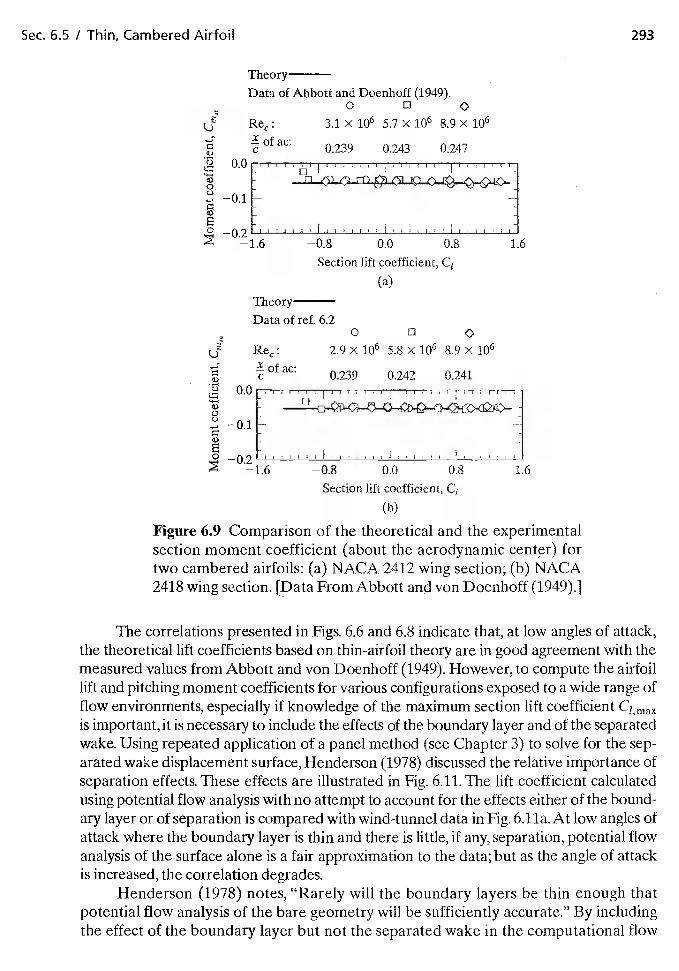
Sec. 6.5 I Thin, Cambered Airfoil 293
Theory
Data of Abbott and Doenhoff (1949).0 0
Ret:of ac:
C
3.1 x 10⁶ 5.7 x 8.9 x 106
.9 0.0
0-0.1
'1)
0—1.6
0.239 0.243 0.247
—0.8 0.0
Section lift coefficient, C1
(a)
0 02.9 X 10⁶ 5.8 x 10⁶ 8.9 x 10⁶
0.239 0.242 0,241
TheoryData of ref. 6,2
ç Ret:
C
0.0
0•-0.1
o —0.2—1.6 —0.8 0.0 0.8 1.6
Section lift coefficient, C1
(b)
Figure 6.9 Comparison of the theoretical and the experimentalsection moment coefficient (about the aerodynamic fortwo cambered airfoils: (a) NACA 2412 wing section; (b) NACA2418 wing section. [Data From Abbott and von Doenhoff (1949).]
The correlations presented in Figs. 6.6 and 6.8 indicate that, at low angles of attack,the theoretical lift coefficients based on thin-airfoil theory are in good agreement with themeasured values from Abbott and von Doenhoff (1949). However, to compute the airfoillift and pitching moment coefficients for various configurations exposed to a wide range offlow environments, especially if knowledge of the maximum section lift coefficient Ci,maxis important, it is necessary to include the effects of the boundary layer and of the separatedwake. Using repeated application of a panel method (see Chapter 3) to solve for the sep-arated wake displacement surface, Henderson (1978) discussed the relative importance ofseparation effects. These effects illustrated in Fig. 6.11. The lift coefficient calculatedusing potential flow analysis with no attempt to account for the effects either of the bound-ary layer or of separation is compared with wind-tunnel data in Fig. 6.1 la. At low angles ofattack where the boundary layer is thin and there is little, if any, separation, potential flowanalysis of the surface alone is a fair approximation to the data; but as the angle of attackis increased, the correlation degrades.
Henderson (1978) notes, "Rarely will the boundary layers be thin enough thatpotential flow analysis of the bare geometry will be sufficiently accurate." By includingthe effect of the boundary layer but not the separated wake in the computational flow
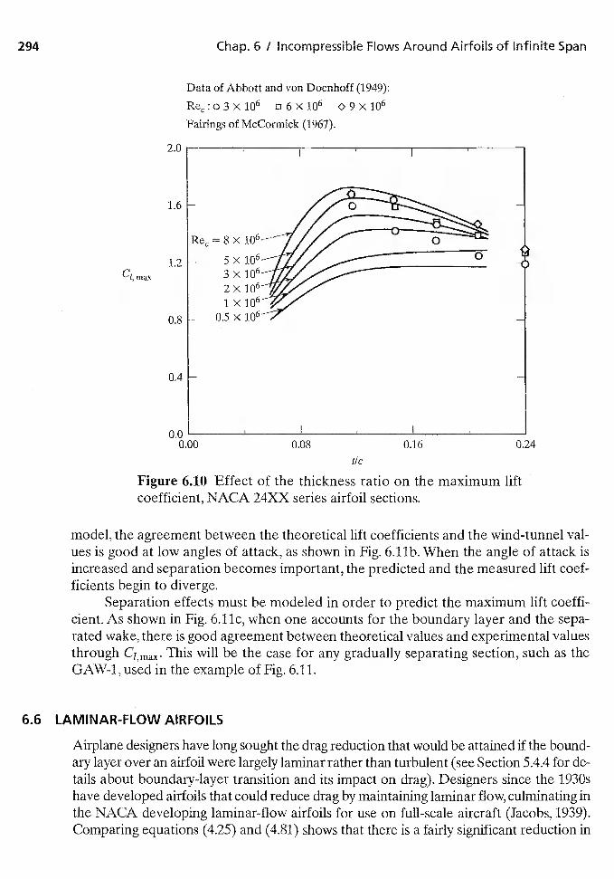
0.8 -
0.4 —
0.0 —0,00
294 Chap. 6 / Incompressible Flows Around Airfoils of Infinite Span
Data of Abbott and von Doenhoff (1949):
06X106Fairings of McCormick (1967).
2.0
1.6 -
= 8 X
1.2 5xCimax 3x
2Xlx
0.5 x
tic
Figure 6.10 Effect of the thickness ratio on the maximum liftcoefficient, NACA 24XX series airfoil sections.
model, the agreement between the theoretical lift coefficients and the wind-tunnel val-ues is good at low angles of attack, as shown in Fig. 6.llb. When the angle of attack isincreased and separation becomes important, the predicted and the measured lift coef-ficients begin to diverge.
Separation effects must be modeled in order to predict the maximum lift coeffi-cient. As shown in Fig. 6.llc, when one accounts for the boundary layer and the sepa-rated wake, there is good agreement between theoretical values and experimental valuesthrough C1, max' Thjs will be the case for any gradually separating section, such as theGAW-1, used in the example of Fig. 6.11.
6.6 LAMINAR-FLOW AIRFOILS
Airplane designers have long sought the drag reduction that would be attained if the bound-ary layer over an airfoil were largely laminar rather than turbulent (see Section 5.4.4 for de-tails about boundary-layer transition and its impact on drag). Designers since the 1930shave developed airfoils that could reduce drag by maintaining laminar flow, culminating inthe NACA developing laminar-flow airfoils for use on full-scale aircraft (Jacobs, 1939).Comparing equations (4.25) and (4.81) shows that there is a fairly significant reduction in
0.08 0.16 0.24
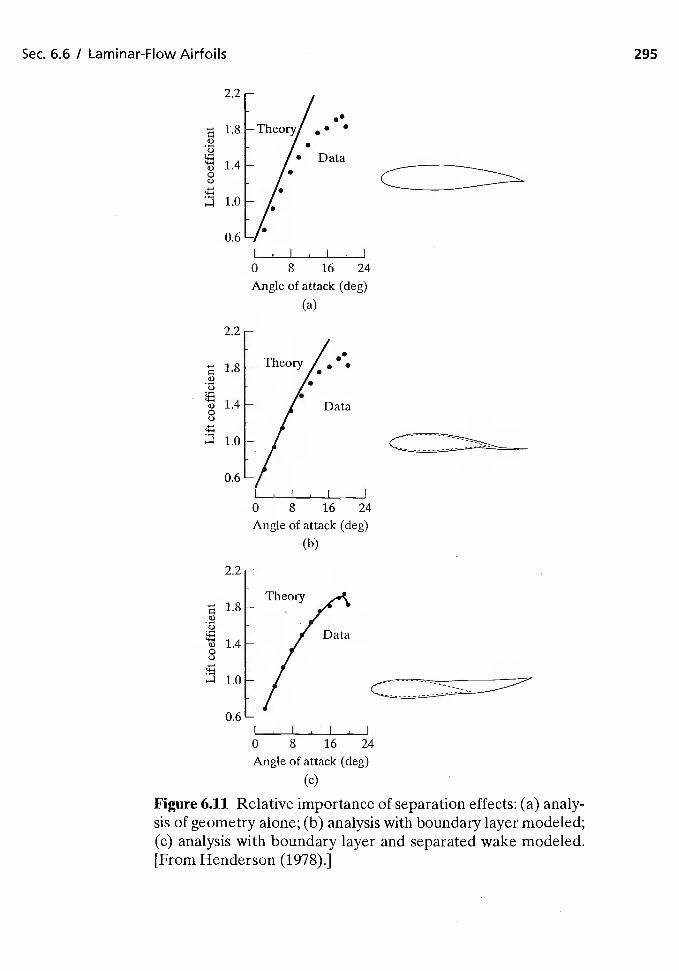
Sec. 6.6 / Laminar-Flow Airfoils 295
1.8a)C-)
a)0C-)
a)C-)
a)0
••
• Data
I I I
0 8 16 24
Angle of attack (deg)(a)
• .
2.2
1.8
1.4
1.0
a)
a)0 Data
0.6I I I
0 8 16 24
Angle of attack (deg)(b)
1.8
1.4
1.0
0.6I I I I
0 8 16 24
Angle of attack (deg)(c)
Figure 6.11 Relative importance of separation effects: (a) analy-sis of geometry alone; (b) analysis with boundary layer modeled;(c) analysis with boundary layer and separated wake modeled.[From Henderson (1978).]
2.2
Theory
Data
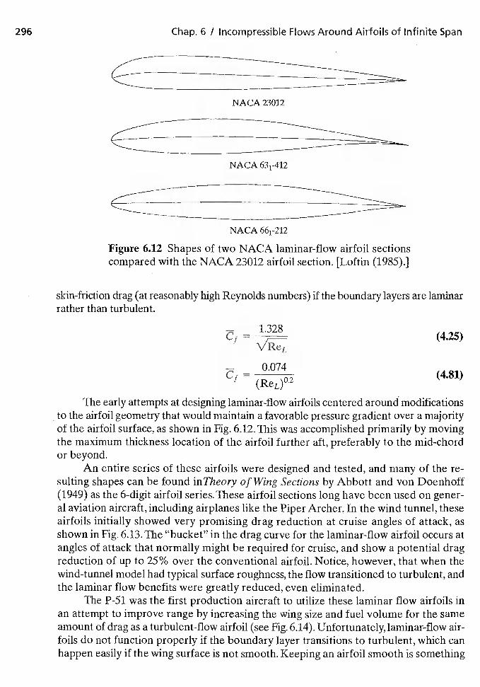
296 Chap. 6 / Incompressible F'ows Around Airfoils of Infinite Span
NACA 23012
NACA
NACA
Figure 6.12 Shapes of two NACA laminar-flow airfoil sectionscompared with the NACA 23012 airfoil section. [Loftin (1985).]
skin-friction drag (at reasonably high Reynolds numbers) if the boundary layers are laminarrather than turbulent.
— 1.328C1
=(4.25)
C = 0.074(4.81)
(ReL)°'2
The early attempts at designing laminar-flow airfoils centered around modificationsto the airfoil geometry that would maintain a favorable pressure gradient over a majorityof the airfoil surface, as shown in Fig. 6.12. This was accomplished primarily by movingthe maximum thickness location of the airfoil further aft, preferably to the mid-chordor beyond.
An entire series of these airfoils were designed and tested, and many of the re-sulting shapes can be found in Theory of Wing Sections by Abbott and von Doenhoff(1949) as the 6-digit airfoil series. These airfoil sections long have been used on gener-al aviation aircraft,including airplanes like the Piper Archer. In the wind tunnel, theseairfoils initially showed very promising drag reduction at cruise angles of attack, asshown in Fig. 6.13,The "bucket" in the drag curve for the laminar-flow airfoil occurs atangles of attack that normally might be required for cruise, and show a potential dragreduction of up to 25% over the conventional airfoil. Notice, however, that when thewind-tunnel model had typical surface roughness, the flow transitioned to turbulent, andthe laminar flow benefits were greatly reduced, even eliminated.
The P-Si was the first production aircraft to utilize these laminar flow airfoils inan attempt to improve range by increasing the wing size and fuel volume for the sameamount of drag as a turbulent-flow airfoil (see Fig. 6.14). Unfortunately, laminar-flow air-foils do not function properly if the boundary layer transitions to turbulent, which canhappen easily if the wing surface is not smooth. Keeping an airfoil smooth is something
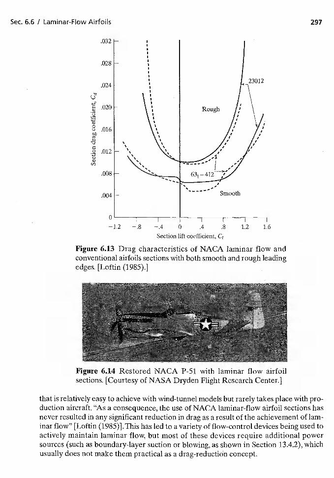
C
0
00
C00
Sec. 6.6 / Laminar-Flow Airfoils 297
.032
.028
.024
.020
23012
.016
Rough
.012
.008
.004
—1.2 —.8 —.4 0 .4 .8
Section lift coefficient, C,
1.2 1.6
Figure 6.13 Drag characteristics of NACA laminar flow andconventional airfoils sections with both smooth and rough leadingedges. [Loftin (1985).]
Figure 6.14 Restored NACA P-51 with laminar flow airfoilsections. [Courtesy of NASA Dryden Flight Research Center.]
that is relatively easy to achieve with wind-tunnel models but rarely takes place with pro-duction aircraft, "As a consequence, the use of NACA laminar-flow airfoil sections hasnever resulted in any significant reduction in drag as a result of the achievement of lam-inar flow" [Loftin (1985)].This has led to a variety of flow-control devices being used toactively maintain laminar flow, but most of these devices require additional powersources (such as boundary-layer suction or blowing, as shown in Section 13.4.2), whichusually does not make them practical as a drag-reductiOn concept.
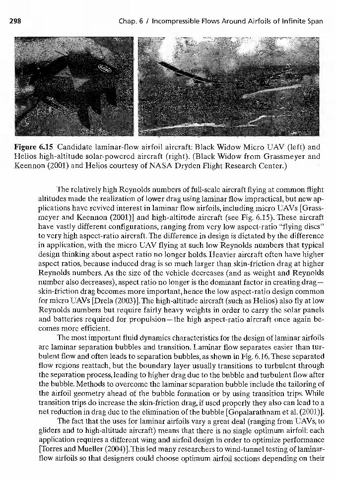
298 Chap. 6 I Incompressible Flows Around Airfoils of Infinite Span
Figure 6.15 Candidate laminar-flow airfoil aircraft:Black Widow Micro UAV (left) andHellos high-altitude solar-powered aircraft (right). (Black Widow from Grassmeyer andKeennon (2001) and Helios courtesy of NASA Dryden Flight Research Center.)
The relatively high Reynolds numbers of full-scale aircraft flying at common flightaltitudes made the realization of lower drag using laminar flow impractical, but new ap-plications have revived interest in laminar flow airfoils, including micro UAVs {Grass-meyer and Keennon (2001)] and high-altitude aircraft (see Fig. 6.15). These aircrafthave vastly different configurations, ranging from very low aspect-ratio "flying discs"to very high aspect-ratio aircraft. The difference in design is dictated by the differencein application, with the micro UAV flying at such low Reynolds numbers that typicaldesign thinking about aspect ratio no longer holds. Heavier aircraft often have higheraspect ratios, because induced drag is so much larger than skin-friction drag at higherReynolds numbers. As the size of the vehicle decreases (and as weight and Reynoldsnumber also decreases), aspect ratio no longer is the dominant factor in creating drag—skin-friction drag becomes more important, hence the low aspect-ratio design commonfor micro UAVs (2003)].The high-altitude aircraft (such as Hellos) also fly at lowReynolds numbers but require fairly heavy weights in order to carry the solar panelsand batteries required for propulsion—the high aspect-ratio aircraft once again be-comes more efficient.
The most important fluid dynamics characteristics for the design of laminar airfoilsare laminar separation bubbles and transition. Laminar flow separates easier than tur-bulent flow and often leads to separation bubbles, as shown in Fig. 6.16. These separatedflow regions reattach, but the boundary layer usually transitions to turbulent throughthe separation process, leading to higher drag due to the bubble and turbulent flow afterthe bubble. Methods to overcome the laminar separation bubble include the tailoring ofthe airfoil geometry ahead of the bubble formation or by using transition trips. Whiletransition trips do increase the skin-friction drag, if used properly they also can lead to anet reduction in drag due to the elimination of the bubble [Gopalarathnam et ad. (2001)].
The fact that the uses for laminar airfoils vary a great deal (ranging from UAVs, togliders and to high-altitude aircraft) means that there is no single optimum airfoil: eachapplication requires a different wing and airfoil design in order to optimize performance[Tortes and Mueller (2004)J.This led many researchers to wind-tunnel testing of laminar-flow airfoils so that designers could choose optimum airfoil sections depending on their
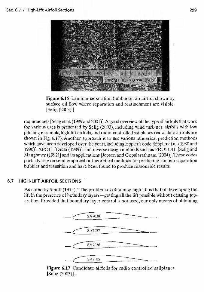
Sec. 6.7 / High-Lift Airfoil Sections 299
Figure 6.16 Laminar separation bubble on an airfoil shown bysurface oil flow where separation and reattachment are visible.[Selig (2003).]
requirements [Selig et al. (1989 and 2001)]. A good overview of the type of airfoils that workfor various uses is presented by Selig (2003), including wind turbines, airfoils with lowpitching moments, high-lift airfoils, and radio-controlled sailplanes (candidate airfoils areshown in Fig. 6.17). Another approach is to use various numerical prediction methodswhich have been developed over the years, including Eppler's code [Eppler et al. (1980 and1990)],XFOIL [Drela (1989)], and inverse design methods such as PROFOIL [Selig andMaughmer (1992)] and its applications [Jepson and Gopalarathnam (2004)].These codespartially rely on semi-empirical or theoretical methods for predicting laminar separationbubbles and transition and have been found to produce reasonable results.
6.7 HIGH-LIFT AIRFOIL SECTIONS
As noted by Smith (1975), "The problem of obtaining high lift is that of developing thelift in the presence of boundary layers—getting all the lift possible without causing sep-aration. Provided that boundary-layer control is not used, our only means of obtaining
Figure 6.17 Candidate airfoils for radio controlled sailpianes.[Selig (2003)].
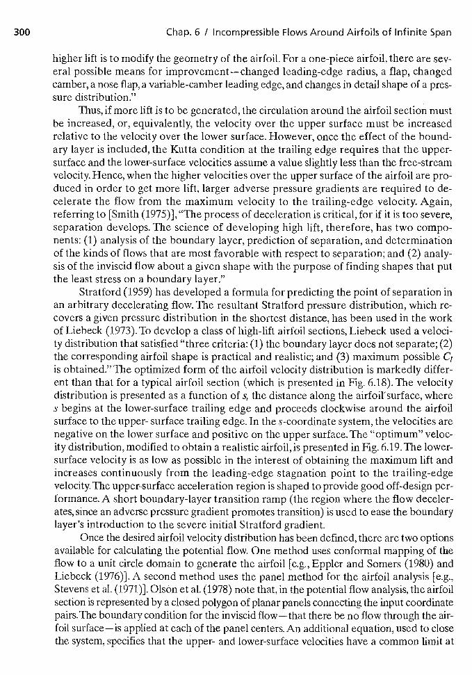
Chap. 6 / Incompressible Flows Around Airfoils of Infinite Span
higher lift is to modify the geometry of the airfoiL For a one-piece airfoil, there are sev-eral possible means for improvement—changed leading-edge radius, a flap, changedcamber, a nose flap, a variable-camber leading edge, and changes in detail shape of a pres-sure distribution."
Thus, if more lift is to be generated, the circulation around the airfoil section mustbe increased, or, equivalently, the velocity over the upper surface must be increasedrelative to the velocity over the lower surface. However, once the effect of the bound-ary layer is included, the Kutta condition at the trailing edge requires that the upper-surface and the lower-surface velocities assume a value slightly less than the free-streamvelocity. Hence, when the higher velocities over the upper surface of the airfoil are pro-duced in order to get more lift, larger adverse pressure gradients are required to de-celerate the flow from the maximum velocity to the trailing-edge velocity. Again,referring to [Smith (1975)], "The process of deceleration is critical, for if it is too severe,separation develops. The science of developing high lift, therefore, has two compo-nents: (1) analysis of the boundary layer, prediction of separatiQn, and determinationof the kinds of flows that are most favorable with respect to separation; and (2) analy-sis of the inviscid flow about a given shape with the purpose of finding shapes that putthe least stress on a boundary layer."
Stratford (1959) has developed a formula for predicting the point of separation inan arbitrary decelerating flow. The resultant Stratford pressure distribution, which re-covers a given pressure distribution in the shortest distance, has been used in the workof Liebeck (1973). To develop a class of high-lift airfoil sections, Liebeck used a veloci-ty distribution that satisfied "three criteria: (1) the boundary layer does not separate; (2)the corresponding airfoil shape is practical and realistic; and (3) maximum possible C1is obtained." The optimized form of the airfoil velocity distribution is markedly differ-ent than that for a typical airfoil section (which is presented in Fig. 6.18). The velocitydistribution is presented as a function of s, the distance along the airfoiY surface, wheres begins at the lower-surface trailing edge and proceeds clockwise around the airfoilsurface to the upper- surface trailing edge. In the s-coordinate system, the velocities arenegative on the lower surface and positive on the upper surface. The "optimum" veloc-ity distribution, modified to obtain a realistic airfoil, is presented in Fig. 6.19.The lower-surface velocity is as low as possible in the interest of obtaining the maximum lift andincreases continuously from the leading-edge stagnation point to the trailing-edgevelocity. The upper-surface acceleration region is shaped to provide good off-design per-formance. A short boundary-layer transition ramp (the region where the flow deceler-ates, since an adverse pressure gradient promotes transition) is used to ease the boundarylayer's introduction to the severe initial Stratford gradient.
Once the desired airfoil velocity distribution has been defined, there are two optionsavailable for calculating the potential flow. One method uses conformal mapping of theflow to a unit circle domain to generate the airfoil [e.g., Eppler and Somers (1980) andLiebeck (1976)], A second method uses the panel method for the airfoil analysis [e.g.,Stevens et al. (1971)]. OlsOn et al. (1978) note that, in the potential flow analysis, the airfoilsection is represented by a closed polygon of planar panels connecting the input coordinatepairs. The boundary condition for the inviscid flow—that there be no flow through the air-foil surface—is applied at each of the panel centers. An additional equation, used to closethe system, specifies that the upper- and lower-surface velocities have a common limit at
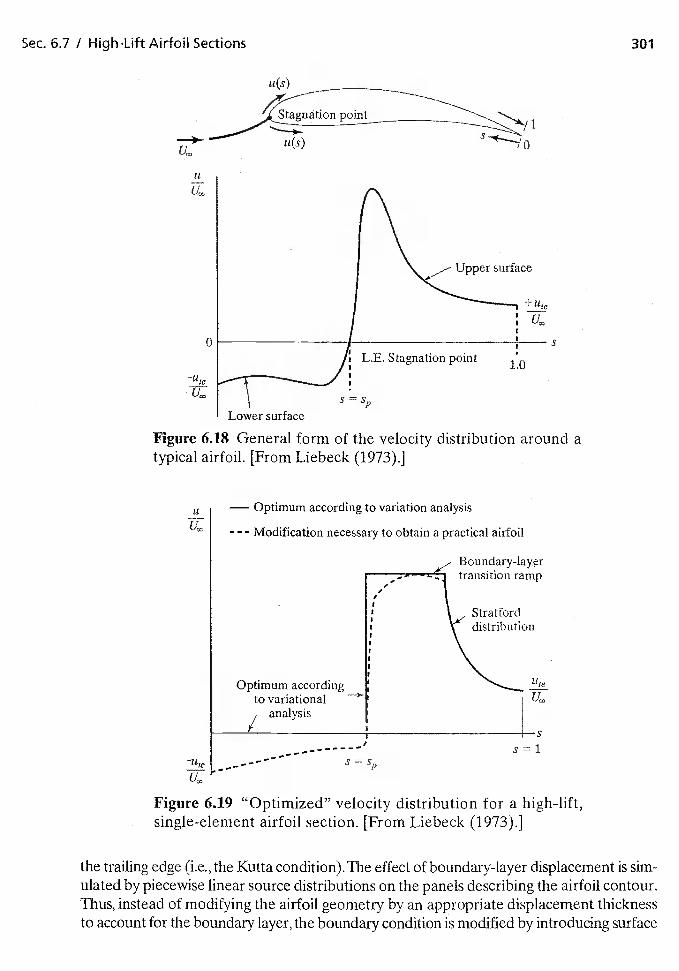
— Optimum according to variation analysis
- -. Modification necessary to obtain a practical airfoil
transition ramp
Upper surface
L.E. Stagnation point
Lower surfaceS =
Sec. 6.7 / High-Lift Airfoil Sections 301
u(s)
S
Ute
Figure 6.18 General form of the velocity distribution around atypical airfoil. [From Liebeck (1973).]
U
,-*—*—-——- s=sp
Figure 6.19 "Optimized" velocity distribution for a high-lift,single-element airfoil section. [From Liebeck (1973).]
the trailing edge (i.e., the Kutta condition). The effect of boundary-layer displacement is sim-ulated by piecewise linear source distributions on the panels describing the airfoil contour.Thus, instead of modifying the airfoil geometry by an appropriate displacement thicknessto account for the boundary layer, the boundary condition is modified by introducing surface
Stratforddistribution
Optimum accordingto variational
/ analysis
tile
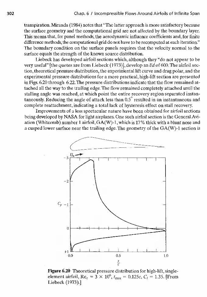
302 Chap. 6 I Incompressible Flows Around Airfoils of Infinite Span
transpiration. Miranda (1984) notes that "The latter approach is more satisfactory becausethe surface geometry and the computational grid are not affected by the boundary layer.This means that, for panel methods, the aerodynamic influence coefficients and, for finitedifference methods, the computational grid do not have to be recomputed at each iteration."The boundary condition on the surface panels requires that the velocity normal to thesurface equals the strength of the known source distribution.
Liebeck has developed airfoil sections which, although they "do not appear to bevery useful" [the quotes are from Liebeck (1973)1, develop an lid of 600.The airfoil sec-tion, theoretical pressure distribution, the experithental lift curve and drag polar, and theexperimental pressure distributions for a more practical, high-lift section are presentedin Figs. 6.20 through 6.22.The pressure distributions indicate that the flow remained at-tached all the way to the trailing edge. The flow remained completely attached until thestalling angle was reached, at which point the entire recovery region separated instan-taneously. Reducing the angle of attack less than 0.5° resulted in an instantaneous andcomplete reattachment, indicating a total lack of hysteresis effect on stall recovery.
Improvements of a less spectacular nature have been obtained for airfoil sectionsbeing developed by NASA for light airplanes. One such airfoil section is the General Avi-ation (Whitcomb) number 1 airfoil, GA(W)-1, which is 17% thick with a blunt nose anda cusped lower surface near the trailing edge. The geometry of the GA(W)-1 section is
—3
—2
—1
0
+10.0 0.5 1.0
xC
Figure 620 Theoretical pressure distribution for high-lift, single-element airfoil, = 3 X tmax = 0.125c, C1 = 1.35. [FromLiebeck (1973).]
U,0
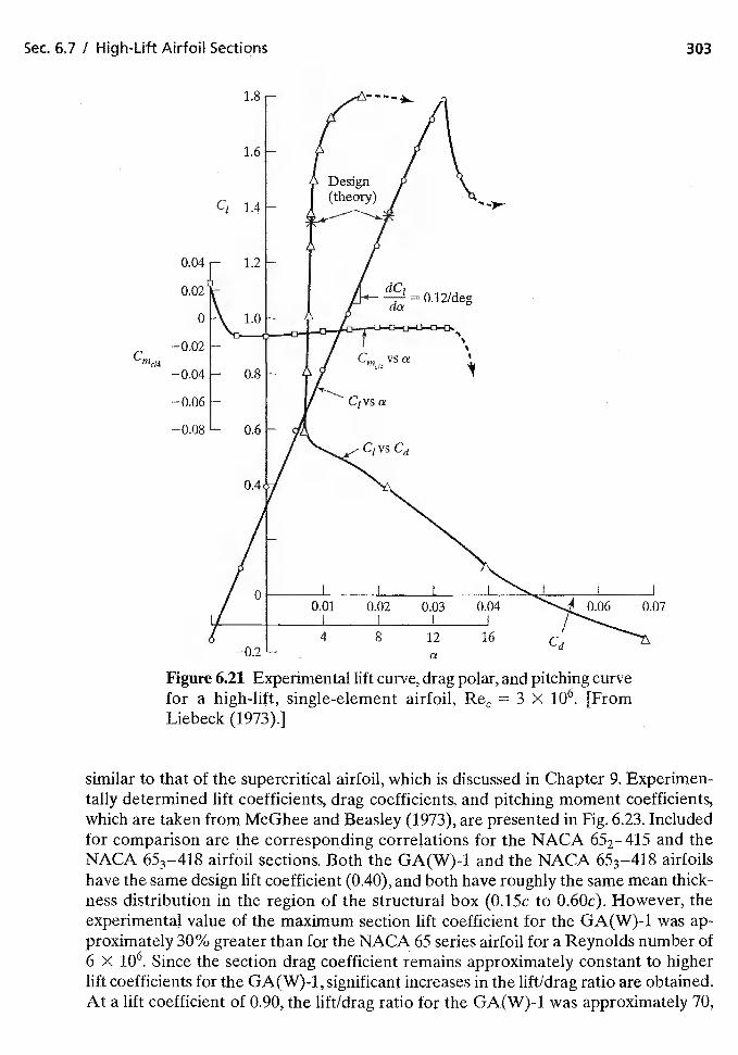
similar to that of the supercritical airfoil, which is discussed in Chapter 9. Experimen-tally determined lift coefficients, drag coefficients, and pitching moment coefficients,which are taken from McGhee and Beasley (1973), are presented in Fig. 6.23. Includedfor comparison are the corresponding correlations for the MACA 652—415 and theNACA 653—418 airfoil sections. Both the GA(W)-1 and the NACA 653—418 airfoilshave the same design lift coefficient (0.40), and both have roughly the same mean thick-ness distribution in the region of the structural box (0.15c to 0.60c). However, theexperimental value of the maximum section lift coefficient for the GA(W)4 was ap-proximately 30% greater than for the NACA 65 series airfoil for a Reynolds number of6 X 106, Since the section drag coefficient remains approximately constant to higherlift coefficients for the GA(W)-1, significant increases in the lift/drag ratio are obtained.At a lift coefficient of 0.90, the lift/drag ratio for the GA(W)-1 was approximately 70,
1.8
1.6
Cl 1,4
Sec. 6.7 / High-LiftAirfoil Sections 303
0.04
0.02
0
—0.02Cm
—0.04
—0.06
—0.08
0.12/deg
C vSa
C1vs a
C1 vs Cd
4
0.03I8 12
a16 Cd
—0.2
Figure 6.21 Experimental lift curve, drag polar, and pitching curvefor a high-lift, single-element airfoil, = 3 X 10⁶. [FromLiebeck (1973).]
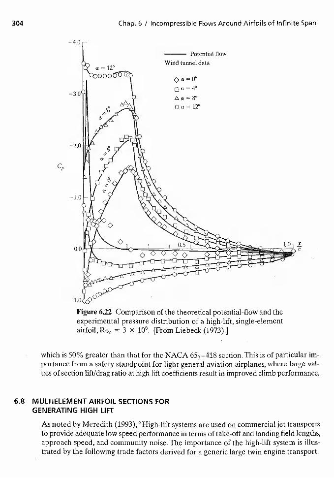
304 Chap. 6 / Incompressible Flows Around Airfoils of Infinite Span
cp
Figure 6.22 Comparison of the theoretical potential-flow and theexperimental pressure distribution of a high-lift, single-elementairfoil, = 3 X 10⁶. [From Liebeck (1973).1
which is 50% greater than that for the NACA 653—418 section. This is of particular im-portance from a safety standpoint for light general aviation airplanes, where large val-ues of section lift/drag ratio at high lift coefficients result in improved climb performance.
6.8 MULTIELEMENT AIRFOIL SECTiONS FORGENERATING HIGH LIFT
As noted by Meredith (1993),"I-Iigh-lift systems are used on commercial jet transportsto provide adequate low speed performance in terms of take-off and landing field lengths,approach speed, and community noise. The importance of the high-lift system is illus-trated by the following trade factors derived for a generic large twin engine transport.
—
—3.0
Potential flow
Wind tunnel data
= 0"
o =4°a = 80
o a 120
xC
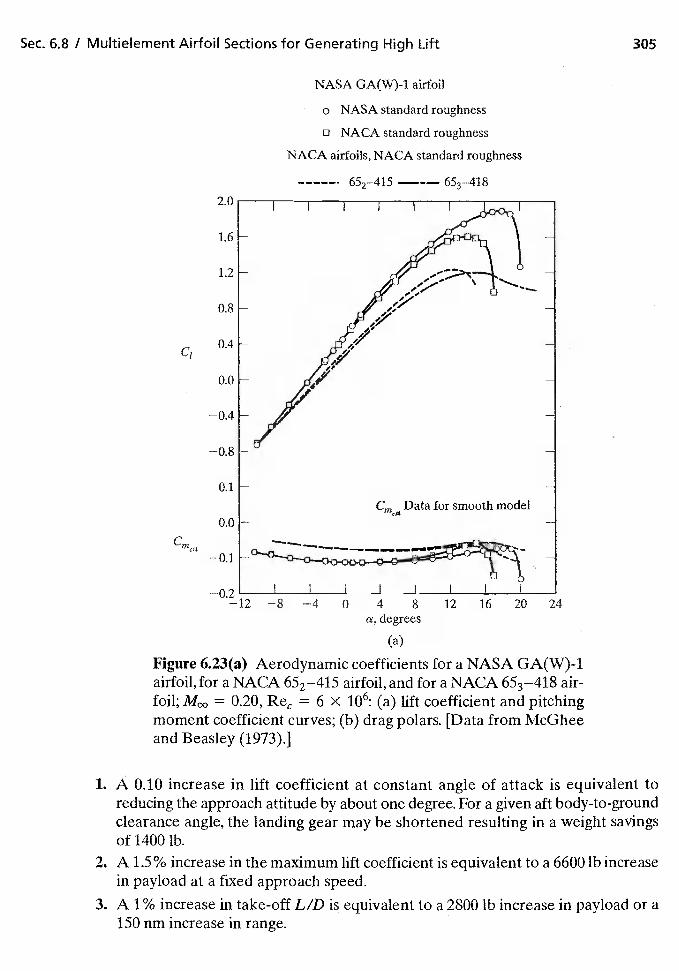
Sec. I Multielement Airfoil Sections for Generating High Lift 305
Cl
NASA GA(W)-1 airfoil
o NASA standard roughness
o NACA standard roughness
NACA airfoils, NACA standard roughness
(a)
Figure 6.23(a) Aerodynamic coefficients for a NASA GA(W)-1airfoil, for a NACA 652—415 airfoil, and for a NACA 653—418 air-foil; = 0.20, = 6 X 10⁶: (a) lift coefficient and pitchingmoment coefficient curves; (b) drag polars. [Data from McGheeand Beasley (1973).]
1. A 0.10 increase in lift coefficient at constant angle of attack is equivalent toreducing the approach attitude by about one degree. For a given aft body-to-groundclearance angle, the landing gear may be shortened resulting in a weight savingsof 1400 lb.
2. A 1,5% increase in the maximum lift coefficient is equivalent to a 6600 lb increasein payload at a fixed approach speed.
3. A 1% increase in take-off LID is equivalent to a 2800 lb increase in payload or a150 nm increase in range.
. 652—415 653—418
a, degrees
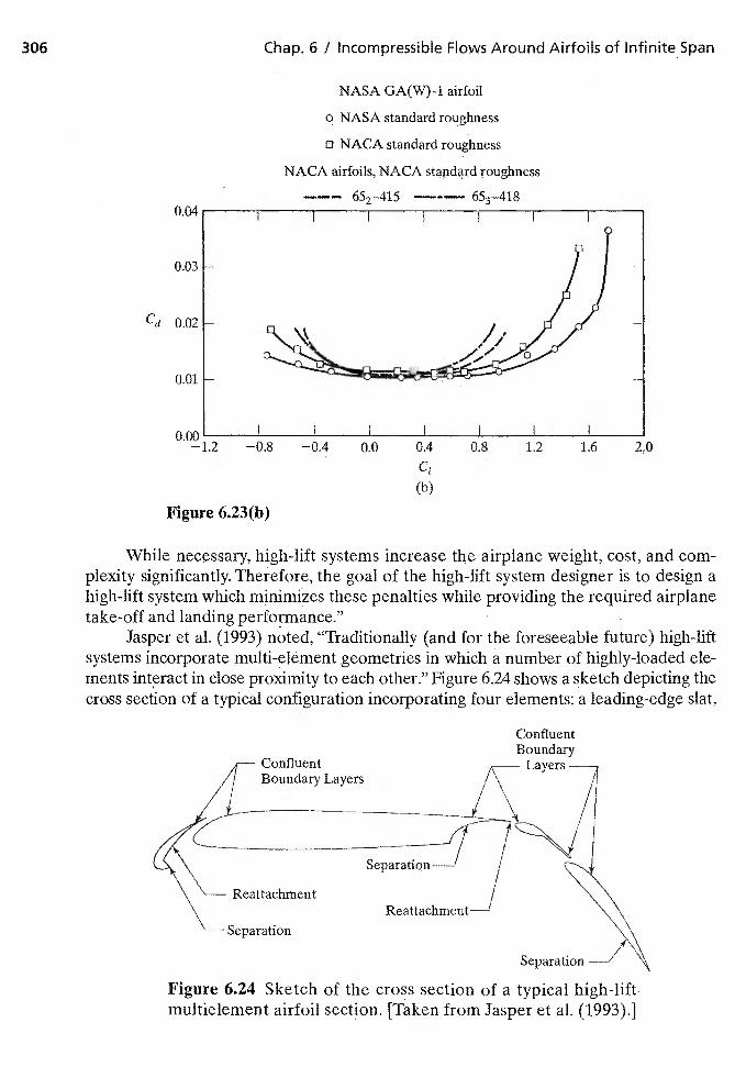
306 Chap. 6 1 Incompressible Flows Around Airfoils of Infinite Span
Figure 6.23(b)
NASA GA(W)-1 airfoil
o NASA standard roughness
o NACA standard roughness
NACA airfoils, NACA standard roughness
652—415 ——— 653—418
0.0 0.4
Cl
(b)
While necessary, high-lift systems increase the airplane weight, cost, and com-plexity significantly. Therefore, the goal of the high-lift system designer is to design ahigh-lift system which minimizes these penalties while providing the required airplanetake-off and landing performance."
Jasper et a!. (1993) noted, "Traditionally (and for the foreseeable future) high-liftsystems incorporate multi-element in which a number of highly-loaded ele-ments interact in close proximity to each other." Figure 6.24 shows a sketch depicting thecross section of a typical configuration incorporating four elements: a leading-edge slat,
Separation
Figure 6.24 Sketch of the cross section of a typical high-liftmultielement airfoil section. [Taken from Jasper et al. (1993).]
0,04 —
0.03 —
Cd 0.02 —
0.01 —
0.00 ——1.2 —0.8 —0.4
I I I I
0.8 1.2 1.6 2,0
ConfluentBoundary Layers
ConfluentBoundary
Layers
Reattachmen t
Separatiqn
Separation
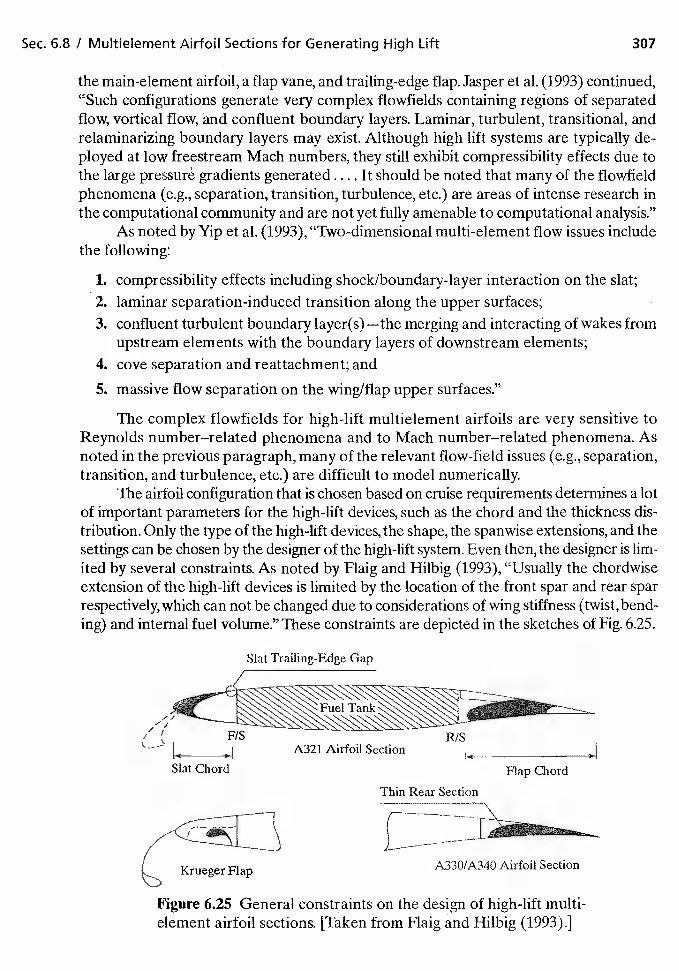
Sec. 6.8 [Multielernent Airfoil Sections for Generating High Lift 307
the main-element airfoil, a flap vane, and trailing-edge flap. Jasper et al. (1993) continued,"Such configurations generate very complex flowfields containing regions of separatedflow, vortical flow, and confluent boundary layers. Laminar, turbulent, transitional, andrelaminarizing boundary layers may exist. Although high lift systems are typically de-ployed at low freestream Mach numbers, they still exhibit compressibility effects due tothe large gradients generated. .. . It should be noted that many of the flowfieldphenomena (e.g., separation, transition, turbulence, etc.) are areas of intense research inthe computational community and are not yet fully amenable to computational analysis."
As noted by Yip eta!. (1993), "Two-dimensional multi-element flow issues includethe following:
1. compressibility effects including shock/boundary-layer interaction on the slat;2. laminar separation-induced transition along the upper surfaces;3. confluent turbulent boundary layer(s) —the merging and interacting of wakes from
upstream elements with the boundary layers of downstream elements;4. cove separation and reattachment; and
S. massive flow separation on the wing/flap upper surfaces."
The complex flowfields for high-lift multielement airfoils are very sensitive toReynolds number—related phenomena and to Mach number—related phenomena. Asnoted in the previous paragraph, many of the relevant flow-field issues (e.g., separation,transition, and turbulence, etc.) are difficult to model numerically.
The airfoil configuration that is chosen based on cruise requirements determines a lotof important parameters for the high-lift devices, such as the chord and the thickness dis-tribution. Only the type of the high-lift devices, the shape, the spanwise extensions, and thesettings can be chosen by the designer of the high-lift system. Even then, the designer is lim-ited by several constraints. As noted by Flaig and Hilbig (1993), "Usually the chordwiseextension of the high-lift devices is limited by the location of the front spar and rear sparrespectively, which can not be changed due to considerations of wing stiffness (twist, bend-ing) and internal fuel volume." These constraints are depicted in the sketches of Fig. 6.25.
Thin Rear Section
A330/A340 Airfoil Section
Figure 6.25 General constraints on the design of high-lift multi-element airfoil sections. [Taken from Flaig and Hilbig (1993) .1
Slat Trailing-Edge Gap
F/SA321 Airfoil Section
R'S
Slat Chord Flap Chord
Krueger Flap
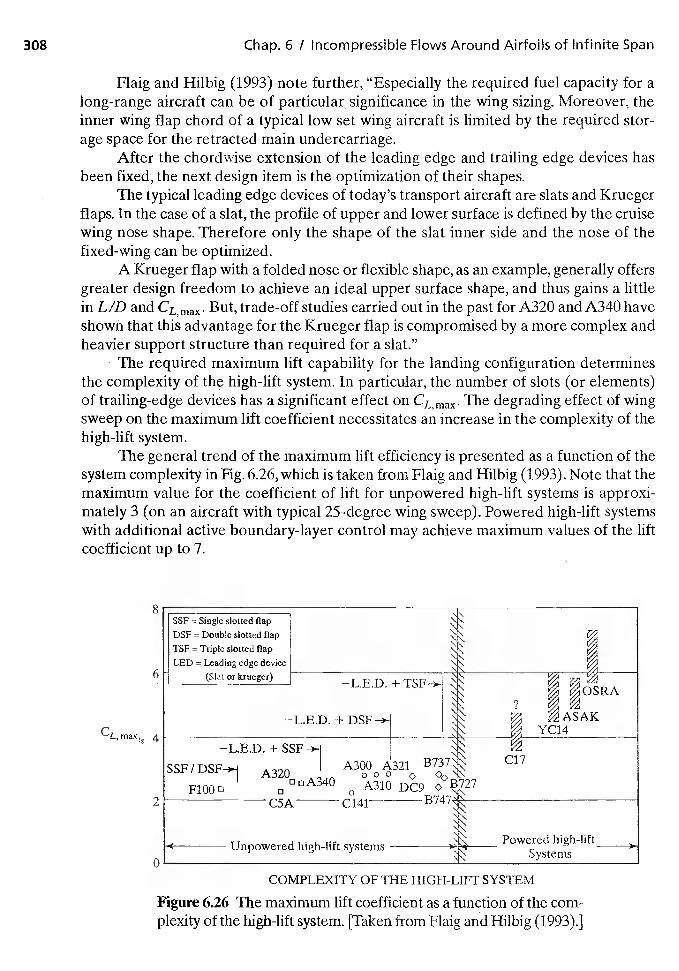
308 Chap. 6 / Incompressible Flows Around Airfoils of Infinite Span
Flaig and Hilbig (1993) note further, "Especially the required fuel capacity for along-range aircraft can be of particular significance in the wing sizing. Moreover, theinner wing flap chord of a typical low set wing aircraft is limited by the required stor-age space for the retracted main undercarriage.
After the chordwise extension of the leading edge and trailing edge devices hasbeen fixed, the next design item is the optimization of their shapes.
The typical leading edge devices of today's transport aircraft are slats and Kruegerflaps. In the case of a slat, the profile of upper and lower surface is defined by the cruisewing nose shape. Therefore only the shape of the slat inner side and the nose of thefixed-wing can be optimized.
A Krueger flap with a folded nose or flexible shape, as an example, generally offersgreater design freedom to achieve an ideal upper surface shape, and thus gains a littlein LID and CL,max. But, trade-off studies carried out in the past for A320 and A340 haveshown that this advantage for the Krueger flap is compromised by a more complex andheavier support structure than required for a slat."
The required maximum lift capability for the landing configuration determinesthe complexity of the high-lift system. In particular, the number of slots (or elements)of trailing-edge devices has a significant effect on CL max The degrading effect of wingsweep on the maximum lift coefficient necessitates an increase in the complexity of thehigh-lift system.
The general trend of the maximum lift efficiency is presented as a function of thesystem complexity in Fig. 6.26, which is taken from Flaig and Hilbig (1993). Note that themaximum value for the coefficient of lift for unpowered high-lift systems is approxi-mately 3 (on an aircraft with typical 25-degree wing sweep). Powered high-lift systemswith additional active boundary-layer control may achieve maximum values of the liftcoefficient up to 7.
8SSF = Single slotted flapDSF = Double slotted flapTSF = Tnple slotted flapLED — Leading edge device
— (Slat or krueger)
—L
—L.E.D. ±
SSF I DSF-*] A320ooA34OFlOOD 0
Unpowered high-hf
+
A300 A321° °A310 DC9
C141
t systems
727
?
C17
4
2
F'
COMPLEXITY OF THE SYSTEM
Figure 6.26 The maximum lift coefficient as a function of the com-plexity of the high-lift system. [Taken from Flaig and Hilbig
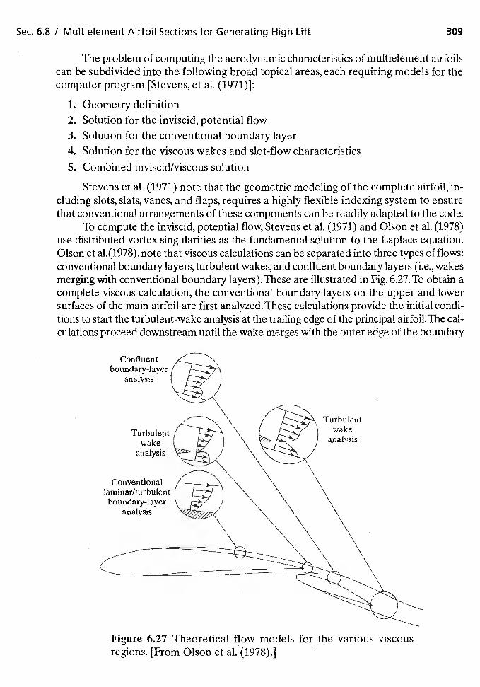
Sec. 6.8 / Multielement Airfoil Sections for Generating High Lift 309
The problem of computing the aerodynamic characteristics of multielement airfoilscan be subdivided into the following broad topical areas, each requiring models for thecomputer program [Stevens, et al. (1971)1:
1. Geometry definition2. Solution for the inviscid, potential flow3. Solution for the conventional boundary layer4. Solution for the viscous wakes and slot-flow characteristics5. Combined inviscid/viscous solution
Stevens et al. (1971) note that the geometric modeling of the complete airfoil, in-cluding slots, slats, vanes, and flaps, requires a highly flexible indexing system to ensurethat conventional arrangements of these components can be readily adapted to the code.
To compute the inviscid, potential flow, Stevens et a!. (1971) and Olson et al. (1978)use distributed vortex singularities as the fundamental solution to the Laplace equation.Olson et al.(1 978), note that viscous calculations can be separated into three types of flows:conventional boundary layers, turbulent wakes, and confluent boundary layers (i.e., wakesmerging with conventional boundary layers).These are illustrated in Fig. 6.27. To obtain acomplete viscous calculation, the conventional boundary layers on the upper and lowersurfaces of the main airfoil are first analyzed, These calculations provide the initial condi-tions to start the turbulent-wake analysis at the trailing edge of the principal airfoil.The cal-culations proceed downstream until the wake merges with the outer edge of the boundary
Figure 6.27 Theoretical flow models for the various viscousregions. [From Olson et al. (1978).]
Confluentboundary-layer
analysis
Turbulentwake
analysis
Conventionallaminar/turbulentboundary-layer
analysis
Turbulentwake
analysis
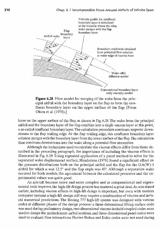
310 Chap. 6 / Incompressible Flows Around Airfoils of Infinite Span
Velocity profile for confluentboundary layer is initializedat the location where the wingwake merges with the flapboundary layer
Boundary conditions obtainedfrom potential-flow solutionat outer edge of viscous zone
Wake eddydiffusion model
Conventional boundary-layereddy viscosity model
Figure 6.28 Flow model for merging of the wake from the prin-cipal airfoil with the boundary layer on the flap to form the con-fluent boundary layer on the upper surface of the flap. [FromOlson et al. (1978).]
layer on the upper surface of the flap, as shown in Fig. 6.28. The wake from the principalairfoil and the boundary layer of the flap combine into a single viscous layer at this point,a so-called confluent boundary layer. The calculation procedure continues stepwise down-stream to the flap trailing edge. At the flap trailing edge, this confluent boundary-layersolution merges with the boundary layer from the lower surface of the flap. The calculationthen continues downstream into the wake along a potential-flow streamline.
Although the techniques used to calculate the viscous effects differ from those de-scribed in the preceding paragraph, the importance of including the viscous effects isillustrated in Fig. 6.29. Using repeated application of a panel method to solve for theseparated wake displacement surface, Henderson (1978) found a significant effect onthe pressure distributions both on the principal airfoil and the flap for the GA(W)-1airfoil for which was 12.5° and the flap angle was 400. Although a separation wakeoccured for both models, the agreement between the calculated pressures and the ex-perimental values was quite good.
As aircraft become more and more complex and as computational and experi-mental tools improve, the high-lift design process has matured a great deal. As was statedearlier, including viscous effects in high-lift design is important, but even with moderncomputer systems a high-lift design still may require a combination of viscous and invis-cid numerical predictions. The Boeing 777 high-lift system was designed with variouscodes at different phases of the design process: a three-dimensional lifting surface codewas used during preliminary design, two-dimensional viscous-inviscid coupled codes wereused to design the multielement airfoil sections, and three-dimensional panel codes wereused to evaluate flow interactions, Navier-Stokes and Euler codes were not used during
Airfoil
N
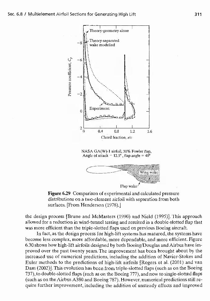
NASA GA(W)-1 airfoil, 30% Fowler flap,Angle of attack = 12.5° , flap angle = 40°
Sec. .6.8 / Multielement Airfoil Sections for Generating High Lift
Theory-geometry alone
Theory-separatedmodelled
0
'1)00
0)
—8
—6
—4
—2
0
20 0.4 0.8 1.2 1.6
Chord fraction, x/c
Flap
Figure 6.29 comparison of experimental and calculated pressuredistributions on a two-element airfoil with separation from bothsurfaces. [From Henderson (1978).]
the design process [Brune and McMasters (1990) and Nield (1995)]. This approachallowed for a reduction in wind-tunnel testing and resulted in a double-slotted flap thatwas more efficient than the triple-slotted flaps used on previous Boeing aircraft.
In fact, as the design process for high-lift systems has matured, the systems havebecome less complex, more affordable, more dependable, and more efficient. Figure6.30 shows how high-lift airfoils designed by both Boeing/Douglas and Airbus have im-proved over the past twenty years. The improvement has been brought about by theincreased use of numerical predictions, including the addition of Navier-Stokes andEuler methods to the predictions of high-lift airfoils [Rogers et al. (2001) and vanDam (2002)].This evolution has been from triple-slotted flaps (such as on the Boeing737), to double-slotted flaps (such as on the Boeing 777), and now to single-slotted flaps(such as on the Airbus A380 and Boeing 787). However, numerical predictions still re-quire further improvement, including the addition of unsteady effects and improved
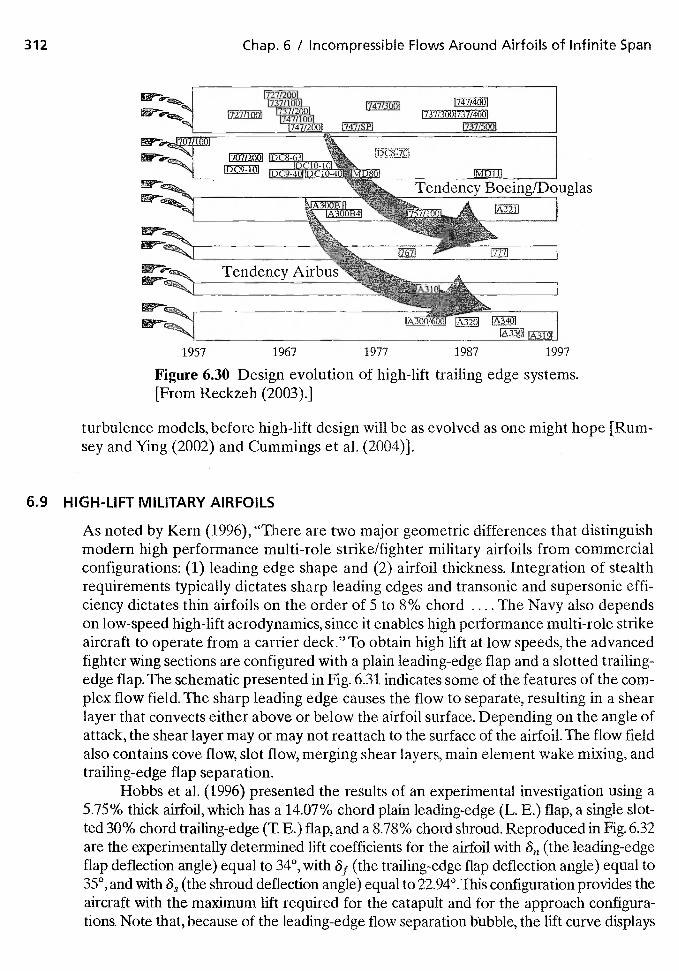
Tendency Boeing/Douglas
1997
Figure 6.30 Design evolution of high-lift trailing edge systems.[From Reckzeh (2003).]
turbulence models, before high-lift design will be as evolved as one might hope [Rum-sey and Ying (2002) and Cummings et al. (2004)].
6.9 HIGH-LIFT MILITARY AIRFOILS
As noted by Kern (1996), "There are two major geometric differences that distinguishmodern high performance multi-role strike/fighter military airfoils from commercialconfigurations: (1) leading edge shape and (2) airfoil thickness. Integration of stealthrequirements typically dictates sharp leading edges and transonic and supersonic effi-ciency dictates thin airfoils on the order of 5 to 8% chord .. . . The Navy also dependson low-speed high-lift aerodynamics, since it enables high performance multi-role strikeaircraft to operate from a carrier deck." To obtain high lift at low speeds, the advancedfighter wing sections are configured with a plain leading-edge flap and a slotted trailing-edge flap. The schematic presented in Fig. 6.31 indicates some of the features of the com-plex flow field. The sharp leading edge causes the flow to separate, resulting in a shearlayer that convects either above or below the airfoil surface. Depending on the angle ofattack, the shear layer may or may not reattach to the surface of the airfoil. The flow fieldalso contains cove flow, slot flow, merging shear layers, main element wake mixing, andtrailing-edge flap separation.
Hobbs et al. (1996) presented the results of an experimental investigation using a5.75% thick airfoil, which has a 14.07% chord plain leading-edge (L. F.) flap, a single slot-ted 30% chord trailing-edge (T. F.) flap, and a 8.78% chord shroud. Reproduced in Fig. 6.32are the experimentally determined lift coefficients for the airfoil with (the leading-edgeflap deflection angle) equal to 34°, with (the trailing-edge flap deflection angle) equal to35°, and with (the shroud deflection angle) equal to 22.94°.This configuration provides theaircraft with the maximum lift required for the catapult and for the approach configura-tions. Note that, because of the leading-edge flow separation bubble, the lift curve displays
312 Chap. 6 / Incompressible Flows Around Airfoils of Infinite Span
r741L300] 1747/400!
!737/300!7371400!
737/500!
Tendency Airbus
1957 1967 1977 1987
A330 !A319!
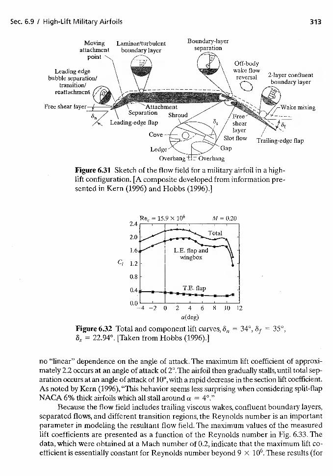
Sec. 6.9 / High-Lift Military Airfoils 313
Overhang tt Overhang
Figure 6.31 Sketch of the flow field for a military airfoil in a high-lift configuration. [A composite developed from information pre-sented in Kern (1996) and Hobbs (1996).]
a(deg)
Figure 6.32 Total and component lift curves, = 34°, 35°,= 22.94°. [Taken from Hobbs (1996).]
no "linear" dependence on the angle of attack. The maximum lift coefficient of approxi-mately 2.2 occurs at an angle of attack of 2°.The airfoil then gradually stalls, until total sep-aration occurs at an angle of attack of 10°, with a rapid decrease in the section lift coefficient.As noted by Kern (1996), "This behavior seems less surprising when considering split-flapNACA 6% thick airfoils which all stall around a = 4°."
Because the flow field includes trailing viscous wakes, confluent boundary layers,separated flows, and different transition regions, the Reynolds number is an importantparameter in modeling the resultant flow field. The maximum values of the measuredlift coefficients are presented as a function of the Reynolds number in Fig. 6.33. Thedata, which were obtained at a Mach number of 0.2, indicate that the maximum lift co-efficient is essentially constant for Reynolds number beyond 9 X 10⁶. These results (for
Moving Laminar/turbulentattachment boundary layer
point
Leading edgebubble separation!
transition!reattachment
Free shear
Off-bodywake flowreversal 2-layer confluent
boundary layer
Attachmentation Shroud
Leading-edge flap
Cove
Ledge
shearlayer
Slot flow
Gap
Wake mixing
Trailing-edge flap
= 15.9>< 106 M = 0.202.4
2.0
1.6
1.2wingbox
_____
T.E. flap0.4 •
0.0 I I I I
—4 —2 0 2 4 6 8 10 12
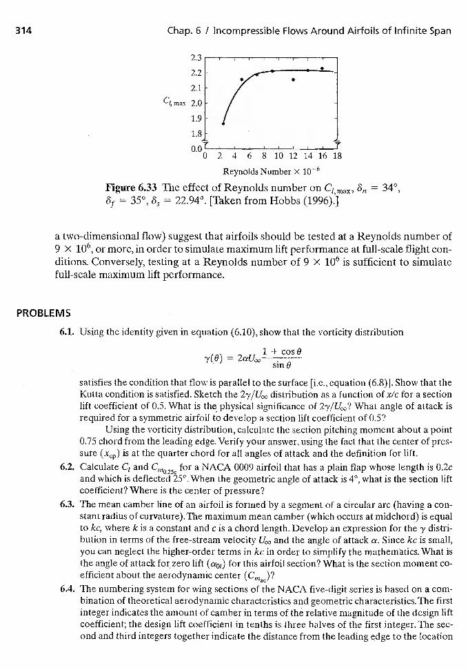
314 Chap. 6 / Incompressible Flows Around Airfoils of Infinite Span
2.0
0 2 4 6 8 10 12 14 16 18
Reynolds Number X
Figure 6.33 The effect of Reynolds number on Cimax, 5,, 34°,= 35°, = 22.94°. [Taken from Hobbs (1996).]
a two-dimensional flow) suggest that airfoils should be tested at a Reynolds number of9 X 106, or more, in order to simulate maximum lift performance at full-scale flight con-ditions. Conversely, testing at a Reynolds number of 9 X 10⁶ is sufficient to simulatefull-scale maximum lift performance.
PROBLEMS
6.1. Using the identity given in equation (6.10), show that the vorticity distribution
1 + cosOy(9) =
sin 0
satisfies the condition that flow is parallel to the surface [i.e., equation (6.8)]. Show that theKutta condition is satisfied. Sketch the distribution as a function of x/c for a sectionlift coefficient of 0,5. What is the physical significance of What angle of attack isrequired for a symmetric airfoil to develop a section lift coefficient of 0.5?
Using the vorticity distribution, calculate the section pitching moment about a point0.75 chord from the leading edge. Verify your answer, using the fact that the center of pres-sure is at the quarter chord for all angles of attack and the definition for lift.
6.2. Calculate C, and Cm025c
for a NACA 0009 airfoil that has a plain flap whose length is O.2cand which is deflected 25°. When the geometric angle of attack is 4°, what is the section liftcoefficient? Where is the center of pressure?
6.3. The mean camber line of an airfoil is formed by a segment of a circular arc (having a con-stant radius of curvature). The maximum mean camber (which occurs at midchord) is equalto kc, where k is a constant and c is a chord length. Develop an expression for the y distri-bution in terms of the free-stream velocity and the angle of attack a. Since kc is small,you can neglect the higher-order terms in kc in order to simplify the mathematics. What isthe angle of attack for zero lift (ao,) for this airfoil section? What is the section moment co-efficient about the aerodynamic center
6.4. The numbering system for wing sections of the NACA five-digit series is based on a com-bination of theoretical aerodynamic characteristics and geometric characteristics. The firstinteger indicates the amount of camber in terms of the relative magnitude of the design liftcoefficient; the design lift coefficient in tenths is three halves of the first integer. The sec-ond and third integers together indicate the distance from the leading edge to the location
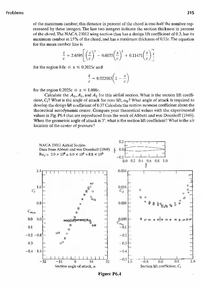
ProHems 315
of the maximum camber; this distance in percent of the chord is one-half the number rep-resented by these integers. The last two integers indicate the section thickness in percentof the chord. The NACA 23012 wing section thus has a design lift coefficient of 0.3, has itsmaximum camber at 15% of the chord, and has a maximum thickness of 0.12c. The equationfor the mean camber line is
= 2.6595[(±) — + 0.11471(i)]
for the region 0.Oc � x � 0.2025c and
= 0.022083(1 —C \. C
for the region O.2025c x � 1.000c.Calculate the A0, A1, and A2 for this airfoil section. What is the section lift coeffi-
cient, C1? What is the angle of attack for zero lift, a01? What angle of attack is required todevelop the design lift coefficient of 0.3? Calculate the section moment coefficient about thetheoretical aerodynamic center. Compare your theoretical values with the experimentalvalues in Fig. P6.4 that are reproduced from the work of Abbott and von Doenhoff (1949).When the geometric angle of attack is 3°,what is the section lift coefficient? What is the x/ciocation of the center of pressure?
NACA 23012 Airfoil SectionData from Abbott and von Doenhoff (1949) 0.0
3.0 X 10⁶ o 6.0 x 10⁶ o 8.8 X 10⁶—0.2
0.0 0.2 0.4 0.6 0.8 1.0xC
2.4 0.024I
-1.6 0.016 °—
C1 C(j 0
0.8 0.008ii
Cm,4
0.0 0.0 .000 B a a
—0.1
00—0.2 —0.8 --0.2
8—0.3 00
—0.4 —1.6 —0.4
—32 —16 16 32 —0.8 0.0 0.8 1.6
Section angle of attack, a Section lift coefficient, C1
Figure P6.4
316 Chap. 6 / Incompressible Flows Around Airfoils of infinite Span
6.5. Look at the three airfoil geometries shown in Fig. 6.12. Discuss the geometric modificationsto the laminar flow airfoils that make them distinct from the typical airfoil (NACA 23012).Include in your description airfoil geometric parameters such as camber, thickness, loca-tion of maximum camber, location of maximum thickness, leading edge radius, and trailingedge shape. Why were these modifications successful in creating a laminar flow airfoil?
6.6. What is a laminar separation bubble? What impact does it have on airfoil aerodynamics?What airfoil design features could be changed to eliminate (or largely reduce) the separa-tion bubble?
6.7. What has enabled the evolution of commercial aircraft high-lift systems from triple-slottedto double- or even single-slotted geometries (see Fig. 6.30)? What are the advantages ofthese changes to aircraft design?
REFERENCES
Abbott IH, von Doenhoff AE. 1949. Theory of Wing Sections. New York: Dover
Brune GW,McMasters JH. 1990. Computational aerodynamics applied to high-lift systems.In ComputationalAerodynamics, Ed. Henne PA. Washington, DC: AIAA
Carison HW, Mack RJ. 1980. Studies of leading-edge thrust phenomena. J. Aircraft17:890—897
Cummings RM, MOrton SA, Forsythe JR. 2004. Detached-eddy simulation of slat and flapaerodynamics for a high-lift wing. Presented at AIAA Aerosp. Sci. Meet., 42nd AIAA Pap.2004—1233, Reno, NV
Drela M. 1989. XFOIL:An analysis and design system for low Reynolds number airfoils. InLow Reynolds Number Aerodynamics, Ed. Mueller TJ. New York: Springer-Verlag
Drela M, Protz JM, Epstein AR 2003. The role of size in the future of aeronautics. Presentedat Infi. Air and Space Symp., AIAA Pap. 2003—2902, Dayton, OH
Eppler R, Somers DM. 1980.A computer program for the design and analysis of low-speedairfoils. NASA Tech. Mem. 80210
Eppler R. 1990. Airfoil Design arid. Data. New York: Springer-Verlag
Flaig A, Hilbig R. 1993. High-lift design for large civil aircraft. In High-Lift System Aero-dynamics, AGARD CP 515
Gopalaratimam A, Broughton BA, McGranahan BD, Selig MS. 2001. Design of low Reynoldsnumber airfoils with trips. Presented at Appi. Aerodyn. Conf., l9th,AIAA Pap. 2001—2463,Anaheim, CA
Grassmeyer JM, Keennon MT. 2001. Development of the Black Widow micro air vehicle.Presented at AIAA Aerosp. Sci. Meet., 39th AIAA Pap. 2001—0127, Reno, NV
Henderson ML. 1978. A solution to the 2-D separated wake modeling problem and its useto predict CLmax of arbitrary airfoil sections. Presented at AIAA Aerosp. Sci. Meet,, 16th,
AIAA Pap. 78—156, Huntsville, AL
Hobbs CR, Spaid FW, Ely WL, Goodman WL. 1996. High lift research program for a fight-er-type, multi-element airfoil at high Reynolds numbers. Presented at AIAA Aerosp. Sci.Meet., AIAA Pap. 96—0057, Reno, NV
Jacobs EN. 1939. Preliminary report on laminar-flow airfoils and new methods adopted forairfoil and boundary-layer investigation. NACA WR L—345
References 317
Jasper DW, Agrawal S, Robinson BA. 1993. Navier-Stokes calculations on multi-elementairfoils using a chimera-based solver. In High-Lift System Aerodynamics, AGARD CF 515
Jepson JK, Gopalarathnam A. 2004. Inverse design of adapative airfoils with aircraft per-formance consideration. Presented at AIAA Aerosp. Sci. Meet., Pap. 2004—0028,Reno, NV
Kern S. 1996. Evaluation of turbulence models for high lift military airfoil flowfields. Pre-sented at AIAA Aerosp. Sci. Meet., 34th, AIAA Pap. 96—0057, Reno, NV
Liebeck RH. 1973. A class of airfoils designed for high lift in incompressible flows. J. Air-craft 10:610—617
Liebeck RH. 1976. On the design of subsonic airfoils for high lift. Presented at Fluid and Plas-ma Dyn. Conf., AIAA Pap. 76—406, San Diego, CA
Loftin LK. 1985. Quest for performance: the evolution of modern aircraft. NASA SP-468
McCormick BW. 1967. Aerodynamics of V/S TO L Flight. New York: Academic Press
McGhee RJ, Beasley WD. 1973. Low-speed aerodynamic characteristics of a 17-percent-thick section designed for general aviation applications. NASA Tech. Note D-7428
Meredith PT. 1993.Viscous phenomena affecting high-lift systems and suggestions for futureCFD Ddevelopment. In High-Lift System Aerodynamics, AGARD CF 515
Miranda LR. 1984. Application of computational aerodynamics to airplane design. J. Air-craft 21:355—369
Nield BN. 1995. An overview of the Boeing 777 high lift aerodynamic design. The Aero-naut. J. 99:361—371
Olson LE, James WD, McGowan PR. 1978. Theoretical and experimental study of thedrag of multieleinent airfoils. Presented at Fluid and Plasma Dyn. Conf., 1 1th, AIAA Pap.78—1223, Seattle, WA
Reckzeh D. 2003.Aerodynamic design of the high-lift wing for a megaliner aircraft.Aerosp.Sci. Tech. 7:107—119
Rogers SE, Roth K, Cao HV, Slotnick JP, Whitlock M, Nash SM, Baker D. 2001. Com-putation of viscous flow for a Boeing 777 aircraft in landing configuration. J. Aircraft38: 1060—1068
Rumsey CL,Ying SX. 2002. Prediction of high lift: review of present CFD capability. Progr.Aerosp. Sci. 38:145—180
Selig MS, Donovan JF, Fraser DB. 1989. Airfoils at Low Speeds. Virginia Beach, VA: HAStokely
Selig MS, Maughmer MD. 1992, A multi-point inverse airfoil design method based on con-formal mapping. AIAA J. 30:1162—1170
Selig MS, Gopalaratham A, Giguére P, Lyon CA. 2001. Systematic airfoil design studies atlow Reynolds number. Jn Fixed and Flapping Wing Aerodynamics for Micro Air VehicleApplications, Ed. Mueller TJ. New York: AIAA, pp. 143—167
Selig MS. 2003. Low Reynolds number airfoil design. In Low Reynolds Number Aerody-namics of Aircraft, VKI Lecture SeriesSmith AMO. 1975. High-lift aerodynamics. J. Aircraft 12:501—530
Stevens WA, Goradia SH, Braden JA. 1971. Mathematical model for two-dimensional multi-component airfoils in viscous flow. NASA CR 1843
318 Chap. 6 / Incompressible Flows Around Airfoils of Infinite Span
Stratford BS. 1959. The prediction of separation of the turbulent boundary layer. J. FluidMech. 5:1-16
Torres GE, Mueller Ti 2004. Low-aspect ratio wing aerodynamics at low Reynolds num-ber. AIAA I. 42:865—873
Van Dam CE 2002.The aerodynamic design of multi-element high-lift systems for transportairplanes. Progr. Aerosp. Sd. 38:101-444
Yip LP,Vijgen PMHW, Hardin JD, van Dam CR 1993. In-flight pressure distributions andskin-friction measurements on a subsonic transport high-lift wing section. In High-Lift Sys-temAerodynamics,AGARD CP515
7 INCOMPRESSIBLE FLOW
ABOUT WINGS
OF FINITE SPAN
7.1 GENERAL COMMENTS
The aerodynamic characteristics for subsonic flow about an unswept airfoil have beendiscussed in Chapters 5 and 6. Since the span of an airfoil is infinite, the flow is identi-cal for each spanwise station (i.e., the flow is two dimensional). The lift produced by thepressure differences between the lower surface and the upper surface of the airfoil sec-tion, and therefore the circulation (integrated along the chord length of the section),does not vary along the span. Foi a wing of finite span, the high-pressure air beneath thewing spills out around the wing tips toward the low-pressure regions above the wing. Asa consequence of the tendency of the pressures acting on the top surface near the tip ofthe wing to equalize with those on the bottom surface, the lift force per unit spandecreases toward the tips. A sketch of a representative aerodynamic load distribution ispresented in Fig. 7.1. As indicated in Fig. 7.la, there is a chordwise variation in the pres-sure differential between the lower surface and the upper surface. The resultant lift forceacting on a section (i.e., a unit span) is obtained by integrating the pressure distributionover the chord length. A procedure that can be used to determine the sectional liftcoefficient has been discussed in Chapter 6.
As indicated in the sketch of Fig. 7.lb, there is a spanwise variation in the lift force.As a result of the spanwise pressure variation, the air on the upper surface flows inboardtoward the root. Similarly, on the lower surface, air will tend to flow outward toward thewing tips. The resultant flow around a wing of finite span is three dimensional, having both
319
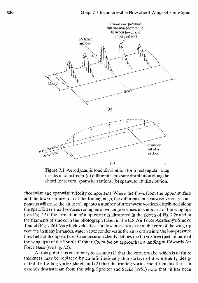
320 Chap. 7 I Incompressible Flow about Wings of Finite Span
Chordwise pressuredistribution (differential
between lower andupper surface)
Figure 71 Aerodynamic load distribution for a rectangular wingin subsonic airstream: differential pressure distribution along thechord for several spanwise stations; (b) spanwise lift distribution.
chordwise and spanwise velocity components. Where the flows from the upper surfaceand the lower surface join at the trailing edge, the difference in spanwise velocity com-ponents will cause the air to roll up into a number of streamwise vortices, distributed alongthe span.These small vortices roll up into two large vortices just inboard of the wing tips(see Fig. 7.2). The formation of a tip vortex is illustrated in the sketch of Fig. 7.2c and inthe filaments of smoke in the photograph taken in the U.S. Air Force Academy's SmokeTunnel (Fig. 7.2d).Very high velocities and low pressures exist at the core of the wing-tipvortices, In many instances, water vapor condenses as the air is drawn into the low-pressureflow field of the tip vortices. Condensation clearly defines the tip vortices (just inboard ofthe wing tips) of the Shuttle Orbiter Columbia on approach to a landing at Edwards AirForce Base (see Fig. 7.3).
At this point, it is customary to assume (1) that the vortex wake, which is of finitethickness, may be replaced by an infinitesimally thin surface of discontinuity, desig-nated the trailing vortex sheet, and (2) that the trailing vortex sheet remains flat as itextends downstream from the wing. Spreiter and Sacks (1951) note that "it has been
Relativeairflow
(a)
(b)
lift at asection
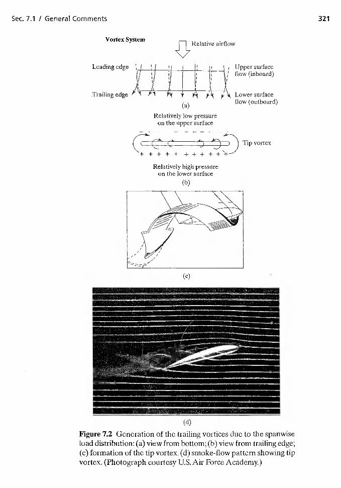
Sec. 7.1 I General Comments 321
Vortex SystemRelative airflow
Leading edge
Trailing edge
Relatively high pressureon the lower surface
(b)
Upper surfaceflow (inboard)
Lower surfaceflow (outboard)
(a)
Relatively low pressureon the upper surface
A—(
)Tip vortex
+ + + + + + + +
(c)
Figure 72 Generation of the trailing vortices due to the spanwiseload distribution: (a) view from bottom; (b) view from trailing edge;(c) formation of the tip vortex. (d) smoke-flow pattern showing tipvortex. (Photograph courtesy U.S. Air Force Academy.)

322 Chap. 7 / Incompressible Flow about Wings of Finite Span
firmly established that these assumptions are sufficiently valid for the prediction of theforces and moments on finite-span wings."
Thus, an important difference in the three-dimensional flow field around a wing(as compared with the two-dimensional flow around an airfoil) is the variationin lift. Since the lift force acting on the wing section at a given spanwise location is relatedto the strength of the circulation, there is a corresponding spanwise variation in circu-lation, such that the circulation at the wing tip is zero. Procedures that can be used todetermine the vortex-strength distribution produced by the flow field around a three-dimensional lifting wing are presented in this chapter.
7.2 VORTEX SYSTEM
A solution is sought for the vortex system which would impart to the surrounding air amotion similar to that produced by a lifting wing. A suitable distribution of vorticeswould represent the physical wing in every way except that of thickness. The vortexsystem consists of
1. The bound vortex system2. The trailing vortex system3. The "starting" vortex
As stated in Chapter 6, the "starting" vortex is associated with a change in circulationand would, therefore, relate to changes in lift that might occur at some time.
Figure 7.3 Condensation marks the wing-tip vortices of the SpaceShuttle Orbiter Columbia. (Courtesy NASA.)
Sec. 7.3 I Lifting-Line Theory for Unswept Wings 323
The representation of the wing by a bound vortex system is not to be interpretedas a rigorous flow model. However, the idea allows a relation to be established between
1. The physical load distribution for the wing (which depends on the wing geometryand on the aerodynamic characteristics of the wing sections)
2. The trailing vortex system
7.3 LIFTING-UNE THEORY FOR UNSWEPT WINGS
For this section, we are interested in developing a model that can be used to estimatethe aerodynamic characteristics of a wing, which is unswept (or is only slightly swept)and which has an aspect ratio of 4.0, or greater. The spanwise variation in lift, 1(y), issimilar to that depicted in Fig. 7.ib. Prandtl and Tietjens (1957) hypothesized that eachairfoil section of the wing acts as though it is an isolated two-dimensional section, pro-vided that the spanwise flow is not too great. Thus, each section of the finite-span winggenerates a section lift equivalent to that acting on a similar section of an infinite-spanwing having the same section circulation. We will assume that the lift acting on anincremental spanwise element of the wing is related to the local circulation through theKutta-Joukowski theorem (see Section 3.15.2).That is,
1(y) = (7.1)
Orloff (1980) showed that the spanwise lift distribution could be obtained from flowfield velocity surveys made behind an airfoil section of the wing only and related to thecirculation around a loop containing that airfoil section.The velocity surveys employedthe integral form of the momentum equation in a manner similar to that used to estimatethe drag in Problems 2.18 through 2.22.
Thus, we shall represent the spanwise lift distribution by a system of vortex fil-aments, the axis of which is normal to the plane of symmetry and which passesthrough the aerodynamic center of the lifting surface. Since the theoretical relationsdeveloped in Chapter 6 for inviscid flow past a thin airfoil showed that the aerody-namic center is at the quarter chord, we shall place the bound-vortex system at thequarter-chord line. The strength of the bound-vortex system at any spanwise loca-tion I(y) is proportional to the local lift acting at that location 1(y). However, asdiscussed in Chapter 3, the vortex theorems of Helrnholtz state that a vortex filamentcannot end in a fluid. Therefore, we shall model the lifting character of the wing bya large number of vortex filaments (i.e., a large bundle of infinitesimal-strength fil-aments) that lie along the quarter chord of the wing. This is the bound-vortex sys-tem, which represents the spanwise loading distribution, as shown in Fig. 7.4(a). Atany spanwise location y, the sum of the strengths of all of the vortex filaments inthe bundle at that station is F(y). When the lift changes at some spanwise location[i.e., the total strength of the bound-vortex system changes proportionally[i.e., But vortex filaments cannot end in the fluid.Thus, the change isrepresented in our model by having some of the filaments from our bundle of fila-ments turn 90° and continue in the streamwise direction (i.e., in the x direction).The strength of the trailing vortex at any y location is equal to the change in thestrength of the bound-vortex system. The strength of the vortex filaments continuing
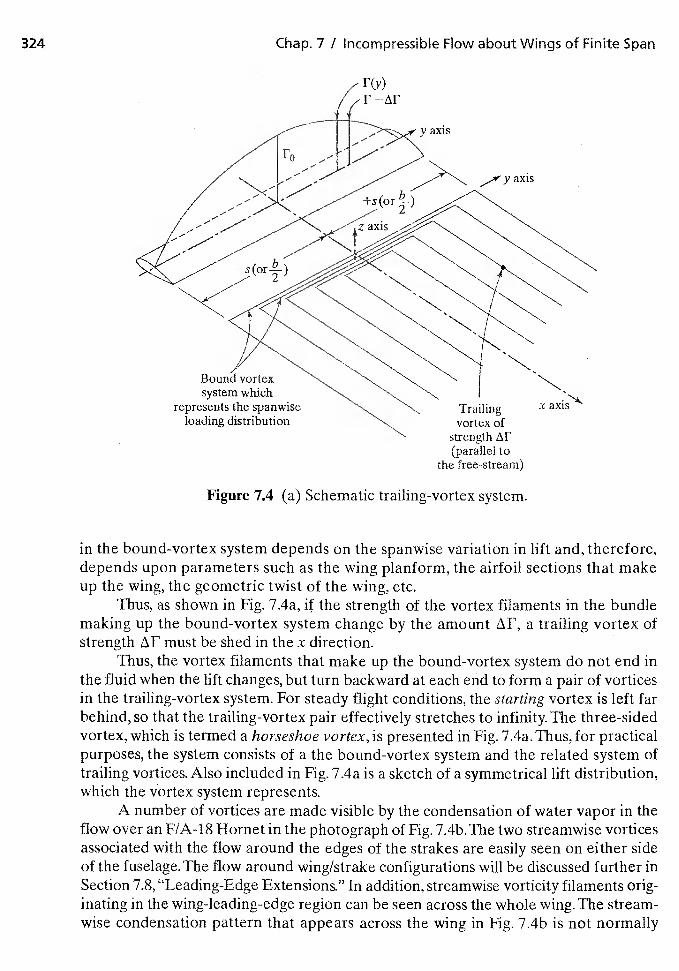
324 Chap. 7 I Incompressible Flow about Wings of Finite Span
Figure 7.4 (a) Schematic trailing-vortex system.
in the bound-vortex system depends on the spanwise variation in lift and, therefore,depends upon parameters such as the wing planform, the airfoil sections that makeup the wing, the geometric twist of the wing, etc.
Thus, as shown in Fig. 7.4a, if the strength of the vortex filaments in the bundlemaking up the bound-vortex system change by the amount a trailing vortex ofstrength must be shed in the x direction.
Thus, the vortex filaments that make up the bound-vortex system do not end inthe fluid when the lift changes, but turn backward at each end to form a pair of vorticesin the trailing-vortex system. For steady flight conditions, the starting vortex is left farbehind, so that the trailing-vortex pair effectively stretches to infinity. The three-sidedvortex, which is termed a horseshoe vortex, is presented in Fig. 7.4a.Thus, for practicalpurposes, the system consists of a the bound-vortex system and the related system oftrailing vortices. Also included in Fig. 7.4a is a sketch of a symmetrical lift distribution,which the vortex system represents.
A number of vortices are made visible by the condensation of water vapor in theflow over an F/A-18 Hornet in the photograph of Fig. 7.4b.The two strearnwise vorticesassociated with the flow around the edges of the strakes are easily seen on either sideof the fuselage. The flow around wing/strake configurations will be discussed further inSection 7.8, "Leading-Edge Extensions." In addition, streamwise vorticity filaments orig-inating in the wing-leading-edge region can be seen across the whole wing. The stream-wise condensation pattern that appears across the wing in Fig. 7.4b is not normally
r(y)r
y axis
axis
vortexsystem which
represents the spanwiseloading distribution
xTrailingvortex of
strength(parallel to
the free-stream)
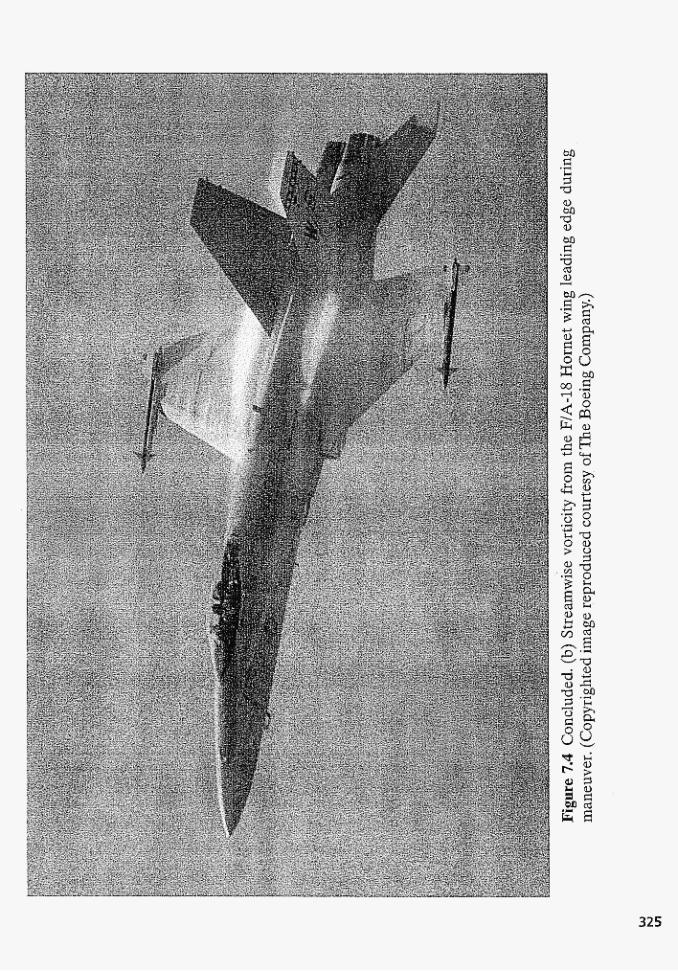
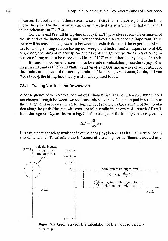
326 Chap. 7 / Incompressible Flow about Wings of Finite Span
observed. It is believed that these streamwise vorticity filaments correspond to the trail-ing vortices shed by the spanwise variation in vorticity across the wing that is depictedin the schematic of Fig. 7.4a.
Conventional Prandtl lifting-line theory (PLLT) provides reasonable estimates ofthe lift and of the induced drag until boundary-layer effects become important. Thus,there will be reasonable agreement between the calculations and the experimental val-ues for a single lifting surface having no sweep, no dihedral, and an aspect ratio of 4.0,or greater, operating at relatively low angles of attack. Of course, the skin friction com-ponent of drag will not be represented in the PLLT calculations at any angle of attack.
Because improvements continue to be made in calculation procedures [e.g., Ras-mussen and Smith (1999) and and Snyder (2000)] and in ways of accounting forthe nonlinear behavior of the aerodynamic coefficients [e.g., Anderson, Corda, and VanWie (1980)], the lifting-line theory is still widely used today.
73.1 Trailing Vortices and Downwash
A consequence of the vortex theorems of Helmholtz is that a bound-vortex system doesnot change strength between two sections unless a vortex filament equal in strength tothe change joins or leaves the vortex bundle. If denotes the strength of the circula-tion along they axis (the spanwise coordinate), a semiinfinite vortex of strength trailsfrom the segment as shown in Fig. 7.5.The strength of the trailing vortex is given by
-
It is assumed that each spanwise strip of the wing (ay) behaves as if the flow were locallytwo dimensional. To calculate the influence of a trailing vortex filament located at y,
yaxisA yaxisf
y =
y=y1 -
Semiinfinite trailing vortex+
I
dFof strength
1
dF is negative in this region for theuy r-distribution of Fig 7.4)
Velocity inducedat y1 by the
trailing vortex/aty
I/
z axis
y = —s
x axis
Figure 7.5 Geometry for the calculation of the induced velocityaty=y1.
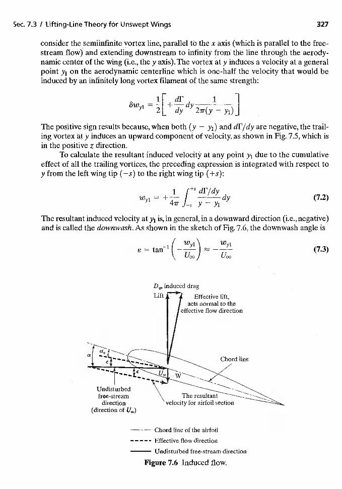
ir 1=[
+ -a-- dy— Yi)
The resultantvelocity for airfoil section
Sec. 7.3 / Lifting-Line Theory fOr Unswept Wings 327
consider the semiinfinite vortex line, parallel to the x axis (which is parallel to the free-streám.flow) and extending downstream to infinity from the line through the aerody-namic center of the wing (i.e., they axis).The vortex at y induces a velocity at a generalpoint y1 on the aerodynamic centerline which is one-half the velocity that would beinduced by an iiifiiiitely long vortex filament of the same strength:
The positive sign results because, when both (y — Yi) and dT'/dy are negative, the trail-ing Vortex at y induces an upward component of velocity, as shown in Fig. 7.5, which isin the positive z direction.
To calculate the resultant induced velocity at any point y1 due to the cumulativeeffect of all the trailing vortices, the preceding expression is integrated with respect toy from the left wing tip (—s) to the right wing tip (+s):
1 dF/dy= +— I dy (7.2)YYi
The resultant induced velocity at y1 is, in general, in a downward direction (i.e., negative)and is called the downwash. As shown in the sketch of Fig. 7.6, the downwash angle is
/ w,1\=
( —(7.3)
induced drag
Lift Effective lift,acts normal to the
effective flow direction
Chord line
Undisturbedfree-stream
direction(direction of U,,,)
— - — Chord line of the airfoil— — — — - Effective flow direction
Undisturbed free-stream direction
Figure 7.6 Induced flow.
328 Chap. 7 I incompressible Flow about Wings of Finite Span
The downwash has the effect of "tilting" the undisturbed air, so the effective angle ofattack at the aerodynamic center (i.e., the quarter chord) is
(7.4)
Note that, if the wing has a geometric twist, both the angle of attack (a) and the down-wash angle (s) would be a function of the spanwise position. Since the direction of theresultant velocity at the aerodynamic center is inclined downward relative to the directionof the undisturbed free-stream air, the effective lift of the section of interest is inclined aftby the same amount. Thus, the effective lift on the wing has a component of force paral-lel to the undisturbed free-stream air (refer to Fig. 7.6). This drag force is a consequenceof the lift developed by a finite wing and is termed vortex drag (or the induced drag or thedrag-due-to-lift). Thus, for subsonic flow past a finite-span wing, in addition to the skinfriction drag and the form (or pressure) drag, there is a drag component due-to-lift. As aresult of the induced downwash velocity, the lift generated by a finite-span wing composedof a given airfoil section, which is at the geometric angle of attack, a, is less than that foran infinite-span airfoil composed of the same airfoil section and which is at the same angleof attack a. See Fig. 5.25. Thus, at a given a, the three-dimensional flow over a finite-spanwing generates less lift than the two-dimensional flow over an infinite-span airfoil.
Based on the Kutta-Joukowski theorem, the lift on an elemental airfoil section ofthe wing is
1(y) = (7.1)
while the vortex drag is(7.5)
The minus sign results because a downward (or negative) value of w produces a posi-tive drag force. Integrating over the entire span of the wing, the total lift is given by
+s
L L dy (7.6)
and the total vortex drag is given by
—f(7.7)
Note that for the two-dimensional airfoil (i.e., a wing of infinite span) the circulationstrength I' is constant across the span (i.e., it is independent of y) and the induced down-wash velocity is zero at all points. Thus, = 0, as discussed in Chapter 6. As a conse-quence of the trailing vortex system, the aerodynamic characteristics are modifiedsignificantly from those of a two-dimensional airfoil of the same section.
7.3.2 Case of Elliptic Spanwise Circulation Distribution
An especially simple circulation distribution, which also has significant practical impli-cations, is given by the elliptic relation (see Fig. 7.7).
F(y) = - (Y)2 (7.8)
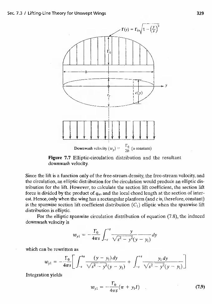
Sec. 7.3 I Lifting-Line Theory for Unswept Wings 329
I H
V
Downwash velocity (wy) = — (a constant)
Figure 7.7 Elliptic-circulation distribution and the resultantdownwash velocity.
Since the lift is a function only of the free-stream density, the free-stream velocity, andthe circulation, an elliptic distribution for the circulation would produce an elliptic dis-tribution for the lift. However, to calculate the section lift coefficient, the section liftforce is divided by the product of and the local chord length at the section of inter-est. Hence, only when the wing has a rectangular planform (and c is, therefore, constant)is the spanwise section lift coefficient distribution (C1) elliptic when the spanwise liftdistribution is elliptic.
For the elliptic spanwise circulation distribution of equation (7.8), the induceddownwash velocity is
WY1=
— Y2(Y — Yi)dy
which can be rewritten as
y1dy
]+ Is Vs2
— y2(Y — Yi)
r(y) =
r [ (y-y1)dy— Li-s Vs2 y2(y — Yl)
Integration yields
F0= —(IT + yi') (7.9)
330 Chap. 7 / Incompressible Flow about Wings of Finite Span
wherep+5j dy
I
_J-s vs—y(y—y1)
Since the elliptic loading is symmetric about the pitch plane of the vehicle (i.e., y = 0),the velocity induced at a point Yi = +a should be equal to the velocity at a point
= —a. Referring to equation (7.9), this can be true if I = 0. Thus, for the elliptic loaddistribution
Wyl = w(y) = (7.10)
The induced velocity is independent of the spanwise coordinate.The total lift for the wing is
L = -
Using the coordinate transformation
y = —scos4
the equation for lift becomes
L f pooUcj0\/1 — cos2 s sin
Thus,
L = = (7.11)
The lift coefficient for the wing is
L ithF0— I c = ')TT
(7.12)
Similarly, we can calculate the total vortex (or induced) drag for the wing.
=-
Introducing the coordinate transformation again, we have
r2 pIT
= JVI — cos2 4 s sin dçb
=(7.13)
and the drag coefficient for the induced component is
r'2I-, — ITI o
1 TT2 ArT2
Sec. 7.3 / Lifting-Line Theory for Unswept Wkigs 331
Rearranging equation (7.12) to solve for gives
(7.15)
Thus,— (2CLUo0S\2
I
'zrb
or
Since the aspect ratio is defined as
b2
C2= L(7.16)irAR
Note that once again we see that the induced drag is zero for a two-dimensional airfoil(i.e., a wing with an aspect ratio of infinity). Note also that the trailing vortex drag foran inviscid flow around a wing is not zero but is proportional to
The induced drag coefficient given by equation (7.16) and the measurements fora wing whose aspect ratio is 5 are compared in Fig. 7.8. The experimental values of theinduced drag coefficient, which were presented by Schlichting and Truckenbrodt (1969),closely follow the theoretical values up to an angle of attack of 20°. The relativelyconstant difference between the measuredvalues and the theoretical values is due tothe influence of skin friction, which was not included in the development of equation(7.16). Therefore, as noted in Chapter 5, the drag coefficient for an incompressible flowis typically written as
CD = CDO + (7.17)
where is the drag coefficient at zero lift and is the lift-dependent drag coeffi-cient. The lift-dependent drag coefficient includes that part of the viscous drag and ofthe form drag, which results as the angle of attack changes from
These relations describing the influence of the aspect ratio on the lift and the draghave been verified experimentally by Prandtl and Betz. If one compares the drag polarsfor two wings which have aspect ratios of AR1 and AR2, respectively, then for a givenvalue of the lift coefficient,
= CD,1 +— AR1)
(7.18)
where CDO,1 has been assumed to be equal to CDO,2. The data from Prandtl (1921) fora series of rectangular wings are reproduced in Fig. 7.9. The experimentally deter-mined drag polars are presented in Fig. 7.9a. Equation (7.18) has been used to con-vert the drag polars for the different aspect ratio wings to the equivalent drag polarfor a wing whose aspect ratio is 5 (i.e., AR2 = 5). These converted drag polars, which
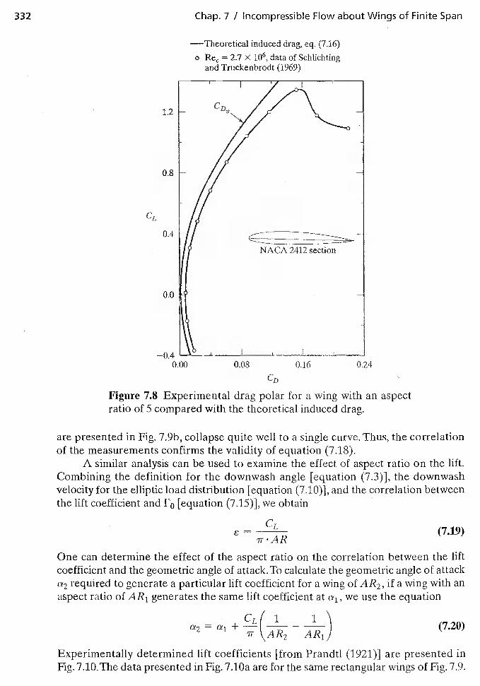
332 Chap. 7 I Incompressible Flow about Wings of Finite Span
—Theoretical induced drag, eq. (7.16)
= 2.7 X 10⁶, data of Schlichtingand Truckenbrodt (1969)
1.2
0.8
CL
0.4
0.0
—0.40.00 0.24
Figure 7.8 Experimental drag polar for a wing with an aspectratio of 5 compared with the theoretical induced drag.
are presented in Fig. 7.9b, collapse quite well to a single curve. Thus, the correlationof the measurements confirms the validity of equation (7.18).
A similar analysis can be used to examine the effect of aspect ratio on the lift.Combining the definition for the downwash angle [equation (7.3)], the downwashvelocity for the elliptic load distribution [equation (7.10)], and the correlation betweenthe lift coefficient and [equation (7.15)], we obtain
CL (719)ir'AR
One can determine the effect of the aspect ratio on the correlation between the liftcoefficient and the geometric angle of attack.To calculate the geometric angle of attacka2 required to generate a particular lift coefficient for a wing of AR2, if a wing with anaspect ratio of AR1 generates the same lift coefficient at a1, we use the equation
a2 = ai + — (7.20)AR1)
Experimentally determined lift coefficients [from Prandtl (1921)] are presented inFig. 7.10. The data presented in Fig. 7.lOa are for the same rectangular wings of Fig. 7.9.
0.08 0.16
CD
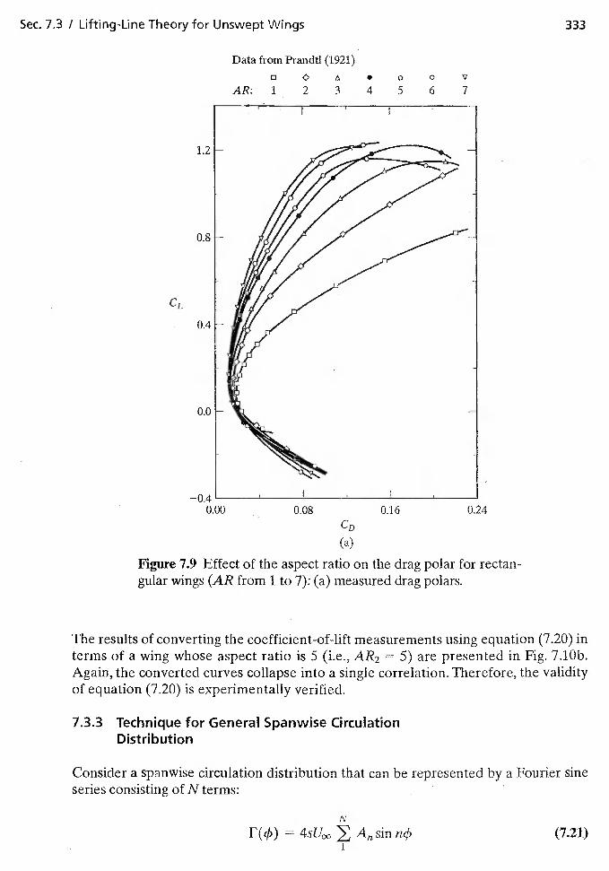
Sec. 7.3 / Lifting-Line Theory for Unswept Wings 333
Data from Prandtl (1921)a
AR: 1 2 3
The results of converting the coefficient-of-lift measurements using equation (7.20) interms of a wing whose aspect ratio is 5 (i.e., AR2 = 5) are presented in Fig. 7.1Db.Again, the converted curves collapse into a single correlation. Therefore, the validityof equation (7.20) is experimentally verified.
7.3.3 Technique for General Spanwise CirculationDistribution
Consider a spanwise circulation distribution that can be represented by a Fourier sineseries consisting of N terms:
N
F(4)
4 5 6
V
7
1.2
0.8 -
0.4 -
CL
—0.4 —0.00
CD
(a)
Figure 7.9 Effect of the aspect ratio on the drag polar for rectan-gular wings (AR from 1 to 7): (a) measured drag polars.
0.08 ft16 0.24
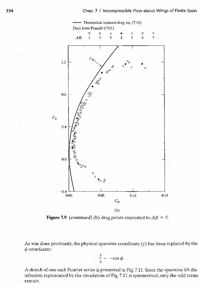
As was done previously, the physical spanwise coordinate (y) has been replaced by the4) coordinate:
y—-=—cos4
A sketch of one such Fourier series is presented in Fig. 7.11. Since the spanwise lift dis-tribution represented by the circulation of Fig. 7.11 is symmetrical, only the odd termsremain.
334 Chap. 7 / Incompressible Flow about Wings of Finite Span
— Theoretical induced drag, eq. (7.16)Data from Prandtl (1921)
0 A • 0 0 V
AR: 1 2 3 4 5 6 7
1.2
0.8
CL
0.4
0.0
—0.40.00 0.08 0.16
CD
0.24
(b)
Figure 7.9 (continued) (b) drag polars converted to AR = 5.
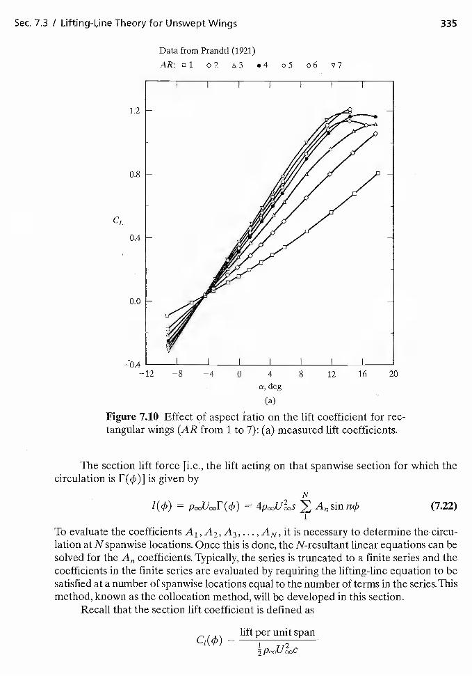
Sec. 7.3 / Lifting-Line Theory for Unswept Wings 335
Data from Prandtl (1921)
AR: ol o2
CL
—0.4 ——12
.4 05 o6 v7
I I
1.2
0.8
0.4
0.0
I I I I I I
—8 —4 0 4 8 12 16 20
a, deg
(a)
Figure 7.10 Effect of aspect ratio on the lift coefficient for rec-tangular wings (AR from 1 to 7): (a) measured lift coefficients.
The section lift force [i.e., the lift acting on that spanwise section for which thecirculation is F(4)] is given by
= sin (7.22)
To evaluate the coefficients A1, A2, A3, . . . ,AN, it is necessary to determine the circu-lation at N spanwise locations. Once this is done, the N-resultant linear equations can besolved for the coefficients. Typically, the series is truncated to a finite series and thecoefficients in the finite series are evaluated by requiring the lifting-line equation to besatisfied at a number of spanwise locations equal to the number of terms in the series.Thismethod, known as the collocation method, will be developed in this section.
Recall that the section lift coefficient is defined as
— lift per unit spanC1(4)—
1 2
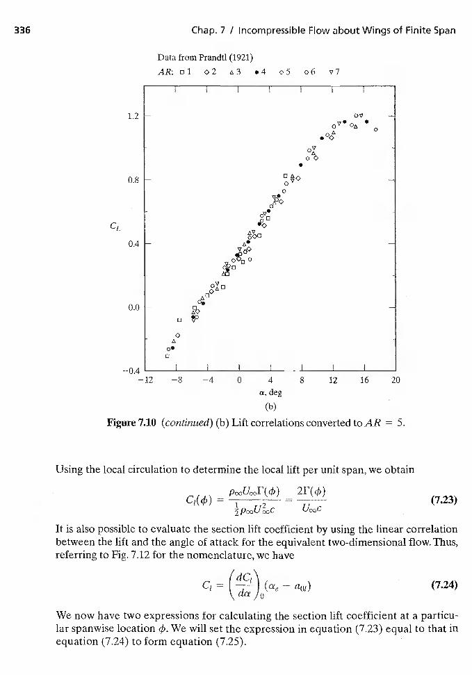
336 Chap. 7 / Incompressible Flow about Wings of Finite Span
Data from Prandtl (1921)
AR: ol o2 .4 o5 o6 v7
I I
1.2 - . .0
.0OX
S
0.8
V5d
CL
0.4V
0
0
0.0—
0
0
——0.4
—12 —8 —4 0 4 8 12 16 20-
(b)
Figure 7.10 (continued) (b) Lift correlations converted to AR = 5.
Using the local circulation to determine the local lift per unit span, we obtain
C1(çb)=
(7.23)
It is also possible to evaluate the section lift coefficient by using the linear correlationbetween the lift and the angle of attack for the equivalent two-dimensional flow. Thus,referring to Fig. 7.12 for the nomenclature, we have
= a01) (7.24)
We now have two expressions for calculating the section lift coefficient at a particu-lar spanwise location We will set the expression in equation (7.23) equal to that inequation (7,24) to form equation (7.25).
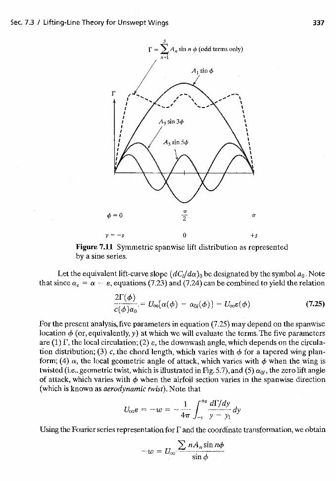
Sec. 7.3 / Lifting-Line Theory for Unswept Wings 337
F = sin n (odd terms only)
y—s 0 +s
Figure 7.11 Symmetric spanwise lift distribution as representedby a sine series.
Let the equivalent lift-curve slope (dC,/da)o be designated by the symbol a0. Notethat since ae = cx — equations (7.23) and (7.24) can be combined to yield the relation
2F(4))/ * aoj(4))] — U00c(4)) (7.25)
For the present analysis, five parameters in equation (7.25) may depend on the spanwiselocation 4) (or, equivalently, y) at which we will evaluate the terms. The five parametersare (1) F, the local circulation; (2) e, the downwash angle, which depends on the circula-tion distribution; (3) c, .the chord length, which varies with 4) for a tapered wing plan-form; (4) a, the local geometric angle of attack, which varies with 4) when the wing istwisted (i.e., geometric twist, which is illustrated in Fig. 5.7), and (5) a01, the zero lift angleof attack, which varies with 4) when the airfoil section varies in the spanwise direction(which is known as aerodynamic twist). Note that
1 dF/dydy
..v — Yi
Using the Fourier series representation for F and the coordinate transformation, we obtain
sin nçb
sm4)
ITIT
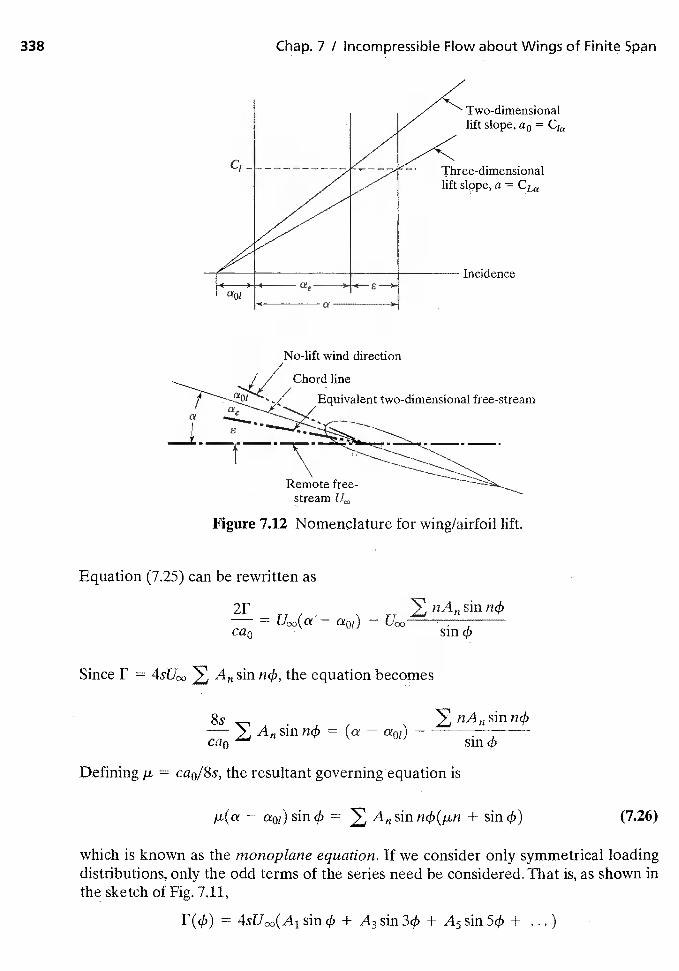
338 Chap. 7 / Incompressible Flow about Wings of Finite Span
Figure 7.12 Nomenclature for wing/airfoil lift.
Equation (7.25) can be rewritten as
21T
ca0
sin n4', the equation becomes
8s .
A,, sin n4sin
Defining p. = cao/8s, the resultant governing equation is
a01) sin A,, sin ncb(/Ln + sin (7.26)
which is known as the monoplane equation. If we consider only symmetrical loadingdistributions, only the odd terms of the series need be considered. That is, as shown inthe sketch of Fig. 7.11,
= + A3 sin 34) + A5 sin 54) +
Cl
Two-dimensionallift slope, a0 = Cia
Incidence
Equivalent two-dimensional free-stream
Remote free-stream
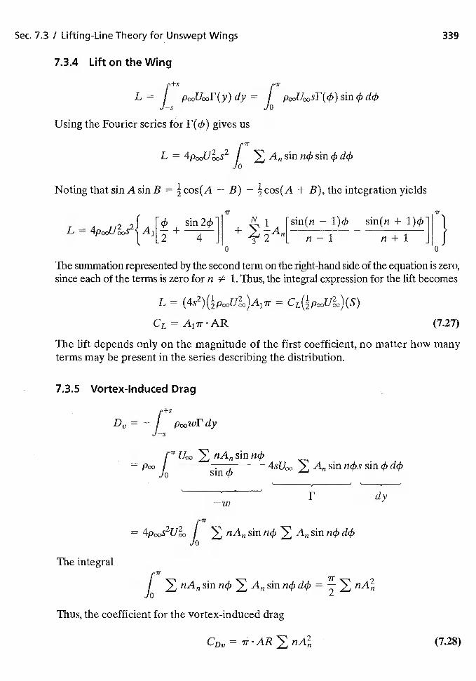
Sec. 7.3 / Lifting-Line Theory for Unswept Wings 339
7.3.4 Lift on the Wing
tIT
L= J J—s 0
Using the Fourier series for F(4) gives us
L = fA sin B = cos(A — B) — cos(A + B), the integration yields
L = + +-
The summation represented by the second term on the right-hand side of the equation is zero,since each of the terms is zero for n 1. Thus, the integral expression for the lift becomes
L = =
CL = A1ir AR (7.27)
The lift depends only on the magnitude of the first coefficient, no matter how manyterms may be present in the series describing the distribution.
7.3.5 Vortex-Induced Drag
f+S
Dv_j pcyjwPdy—S
sin nq5PooJ
F dy
= f sin sin nç& dçb
The integral
fThus, the coefficient for the vortex-induced drag
= 7nAR (7.28)
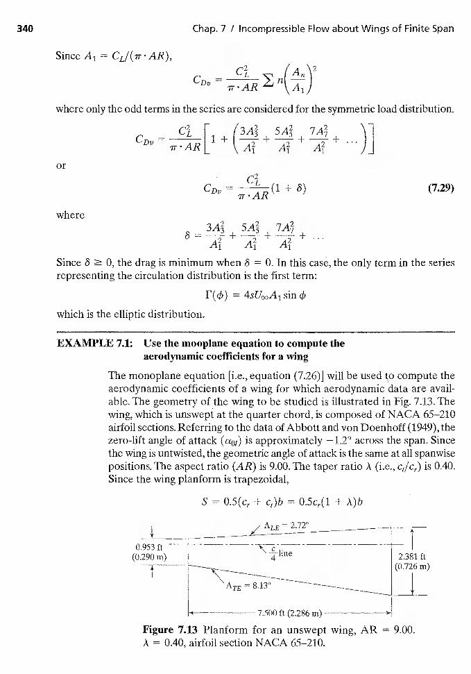
340 Chap. 7 / Incompressible Flow about Wings of Finite Span
Since A1 CL/(ITAR),
CDV=
where only the odd terms in the series are considered for the symmetric load distribution.
[CDV=
7r.ARLor
C2=•AR
(1 + 6) (7.29)
where
42 42 42P11 111
Since 6 � 0, the drag is minimum when 6 0. In this case, the only term in the seriesrepresenting the circulation distribution is the first term:
=
which is the elliptic distribution.
EXAMPLE 7.1: Use the mooplane equation to compute theaerodynamic coefficients for a wing
The monoplane equation [i.e., equation (7.26)] will be used to compute theaerodynamic coefficients of a wing for which aerodynamic data are avail-able. The geometry of the wing to be studied is illustrated in Fig. 7.13. Thewing, which is unswept at the quarter chord, is composed of NACA 65—210airfoil sections. Referring to the data of Abbott and von Doenhoff (1949), thezero-lift angle of attack (a01) is approximately —1.2° across the span. Sincethe wing is untwisted, the geometric angle of attack is the same at all spanwisepositions. The aspect ratio (AR) is 9.00. The taper ratio A (i.e., Ct/Cr) is 0.40.Since the wing planform is trapezoidal,
S = 0.5(Cr + c,)b 0.5Cr(1 + A)b
ALE = 2.720
1
(0290 2381 ft
7.500 ft (2.286 m)
Figure 7.13 Planform for an unswept wing, AR = 9.00.A = 0.40, airfoil section NACA 65—210.
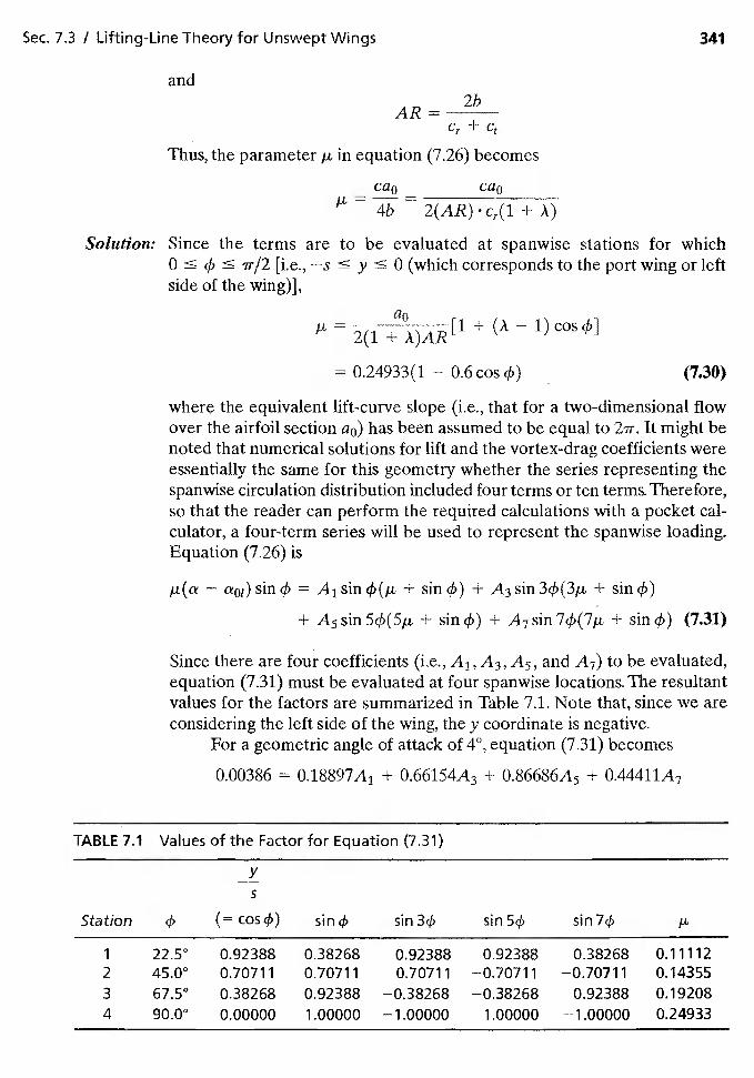
Sec. 7.3 / Lifting-Line Theory for Unswept Wings 341
and
AR= 2b
Cr +
Thus, the parameter in equation (7.26) becomes
Ca0 Ca0
= 4b = 2(AR)Cr(1 + A)
Solution: Since the terms are to be evaluated at spanwise stations for whicho � � ir/2 [i.e., —s < y 0 (which corresponds to the port wing or leftside of the wing)J,
= 2(1+ (A — 1)cos4)]
= 0.24933(1 — 0.6cos4)) (7.30)
where the equivalent lift-curve slope (i.e., that for a two-dimensional flowover the airfoil section a0) has been assumed to be equal to 2ir. It might benoted that numerical solutions for lift and the vortex-drag coefficients wereessentially the same for this geometry whether the series representing thespanwise circulation distribution included four terms or ten terms. Therefore,so that the reader can perform the required calculations with a pocket cal-culator, a four-term series will be used to represent the spanwise loading.Equation (7.26) is
— = + sin4)) + + sin4))
+ A5 sin 54)(Sji + sin 4)) + A7 sin + sin 4)) (731)
Since there are four coefficients (i.e., A1, A3, A5, and A7) to be evaluated,equation (7.31) must be evaluated at four spanwise locations. The resultantvalues for the factors are summarized in Table 7.1. Note that, since we areconsidering the left side of the wing, the y coordinate is negative.
For a geometric angle of attack of 40, equation (7.31) becomes
0.00386 = 0.18897A1 + 0.66154A3 + 0.86686A5 + 0.44411A7
TABLE 7.1 Values of the Factor for Equation (7.31)
yS
Station (/1 (= cos4)) sin4) sin 34) sin 54) sin 74)
1 22.5° 0.92388 0.38268 0.92388 0.92388 0.38268 0.111122 45.0° 0.70711 0.70711 0.70711 —0.70711 —0.70711 0.143553 67.5° 0.38268 0.92388 —0.38268 —0.38268 0.92388 0.192084 90.0° 0.00000 1.00000 — 1.00000 1.00000 1.00000 0.24933
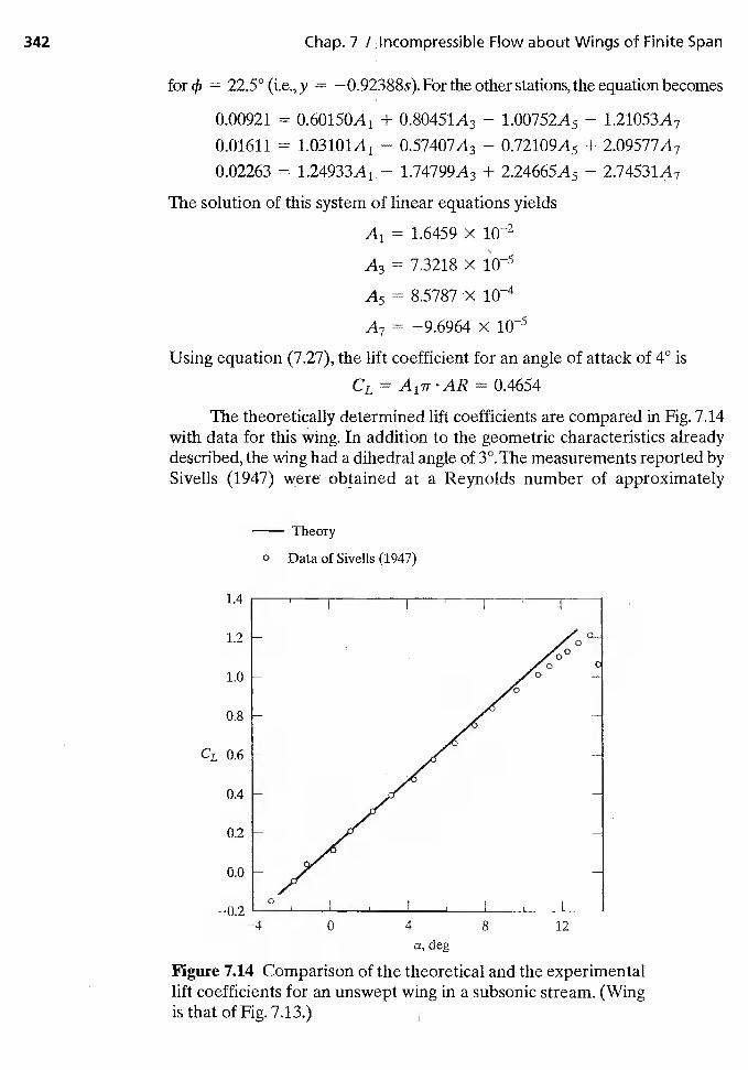
342 Chap. 7 / Incompressible Flow about Wings of Finite Span
for = 22.5° (i.e., y = —0.92388s). For the other stations, the equation becomes
0.00921 = 0.60150A1 + 0.80451A3 — 1.00752A5 — 1.21053A7
0.01611 = 1.03101A1 — 0.57407A3 — 0.72109A5 + 2.09577A7
0.02263 = 1.24933A1 1,74799A3 + 2.24665A5 — 2.74531A7
The solution of this system of linear equations yields
A1 = 1.6459 x
A3 = 7.3218 x
A5 = 8.5787
x
Using equation (7.27), the lift coefficient for an angle of attack of 4° is
CL A1Tr AR = 0.4654
The theoretically determined lift coefficients are compared in Fig. 7.14with data for this wing. In addition to the geometric characteristics alreadydescribed, the wing had a dihedral angle of 3°, The measurements reported bySivells (1947) were obtained at a Reynolds number of approximately
—0.2
— Theory0 Data of Sivells (1947)
a, deg
Figure 714 Comparison of the theoretical and the experimentallift coefficients for an unswept wing in a subsonic stream. (Wingis that of Fig. 7.13.)
0
1.4
1.2 —
1.0 -
0.8
CL 0.6
0.4
0.2
0.0
0
0
—4 0 4 8 12
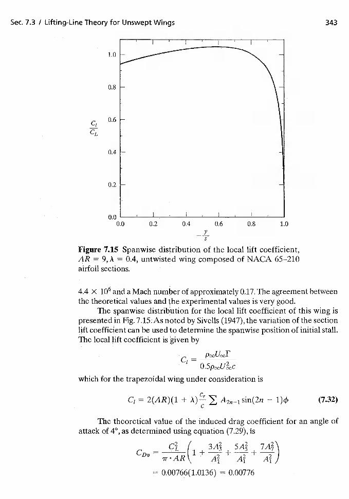
0.4 0.6 0.8 1.0
Figure 7.15 Spanwise distribution of the local lift coefficient,AR = 9, A = 0.4, untwisted wing composed of NACA 65--210airfoil sections.
4.4 X 10⁶ and a Mach number of approximately 0.17. The agreement betweenthe theoretical values and the experimental values is very good.
The spanwise distribution for the local lift coefficient of this wing ispresented in Fig. 7.15:As noted by Sivells (1947), the variation of the sectionlift coefficIent can be used to determine the spanwise position of initial stall.The local lift coefficient is given by
Cl—
which for the trapezoidal wing under consideration is
2(AR)(1 + sin(2n — (7.32)
The theoretical value of the induced drag coefficient for an angle ofattack of 4°, as determined using equation (7.29), is
/CDV=
= 0.00766(1.0136) = 0.00776
343Sec. 7.3 / Lifting-Line Theory for Unswept Wings
1.0
0.8
0.6
CL
0.4
0.2
0.00.0 0.2
yS
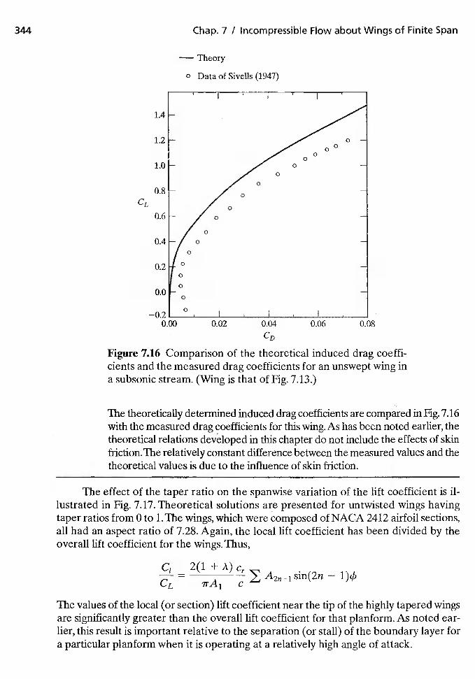
344 Chap. 7 / Incompressible Flow about Wings of Finite Span
CL
— Theory
0 Data of Sivells (1947)
Figure 7.16 Comparison of the theoretical induced drag coeffi-cients and the measured drag coefficients for an unswept wing ina subsonic stream. (Wing is that of Fig. 7.13.)
The theoretically determined induced drag coefficients are compared in Fig. 7.16with the measured drag coefficients for this wing. As has been noted earlier, thetheoretical relations developed in this chapter do not include the effects of skinfriction. The relatively constant difference between the measured values and thetheoretical values is due to the influence of skin friction.
The effect of the taper ratio on the spanwise variation of the lift coefficient is ii-lustrated in Fig. 7.17. Theoretical solutions are presented for untwisted wings havingtaper ratios from 0 to 1.The wings, which were composed of NACA 2412 airfoil sections,all had an aspect ratio of 7.28. Again, the local lift coefficient has been divided by theoverall lift coefficient for the wings. Thus,
C1 2(1+A)c=
sin(2n — 1)4
The values of the local (or section) lift coefficient near the tip of the highly tapered wingsare significantly greater than the overall lift coefficient for that planform. As noted ear-lier, this result is important relative to the separation (or stall) of the boundary layer fora particular planform when it is operating at a relatively high angle of attack.
0.04
CD
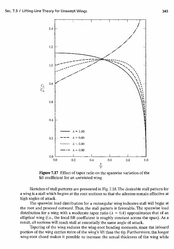
Figure 7.17 Effect of taper ratio on the spanwise variation of thelift coefficient for an untwisted wing.
Sketches of stall patterns are presented in Fig. 7.18. The desirable stall pattern fora wing is a stall which begins at the root sections so that the ailerons remain effective athigh angles of attack.
The spanwise load distribution for a rectangular wing indicates stall will begin atthe root and proceed outward. Thus, the stall pattern is favorable. The spanwise loaddistribution for a wing with a moderate taper ratio (A = 0.4) approximates that of anelliptical wing (i.e., the local lift coefficient is roughly constant across the span). As aresult, all sections will reach stall at essentially the same angle of attack.
Tapering of the wing reduces the wing-root bending moments, since the inboardportion of the wing carries more of the wing's lift than the tip. Furthermore, the longerwing-root chord makes it possible to increase the actual thickness of the wing while
Sec. 7.3 I Lifting-Line Theory for Unswept Wings 345
1.4
1.2
1.0
0.8Cl
CL
0.6
0.4
0.2
0.00.0 0.2 0.4 0.6 0.8
yS
1.0
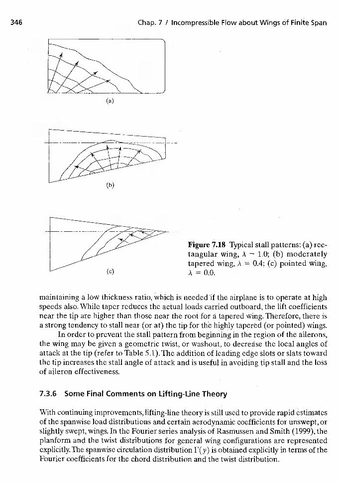
346 Chap. 7 / Incompressible Flow about Wings of Finite Span
Figure 7.18 Typical stall patterns: (a) rec-tangular wing, A = 1.0; (b) moderatelytapered wing, A = 0.4; (c) pointed wing,A = 0.0,
maintaining a low thickness ratio, which is needed if the airplane is to operate at highspeeds also. While taper reduces the actual loads carried outboard, the lift coefficientsnear the tip are higher than those near the root fOr a tapered wing. Therefore, there isa strong tendency to stall near (or at) the tip for the highly tapered (or pointed) wings.
In order to prevent the stall pattern from beginning in the region of the ailerons,the wing may be given a geometric twist, Or washout, to decrease the local angles ofattack at the tip (refer to Table 5.1).The addition of leading edge slots or slats towardthe tip increases the stall angle of attack and is useful in avoiding tip stall and the lossof aileron effectiveness.
7.3.6 Some Final Comments on Lifting-Line Theory
With continuing improvements, lifting-line theory is still used to provide rapid estimatesof the spanwise load distributions and certain aerodynamic coefficients for unswept, orslightly swept, wings. In the Fourier series analysis of Rasmussen and Smith (1999), theplanform and the twist distributions for general wing configurations are representedexplicitly. The spanwise circulation distributiOn F(y) is obtained explicitly in terms of theFourier coefficients for the chord distribution and the twist distribution.
(a)
(b)
(c)
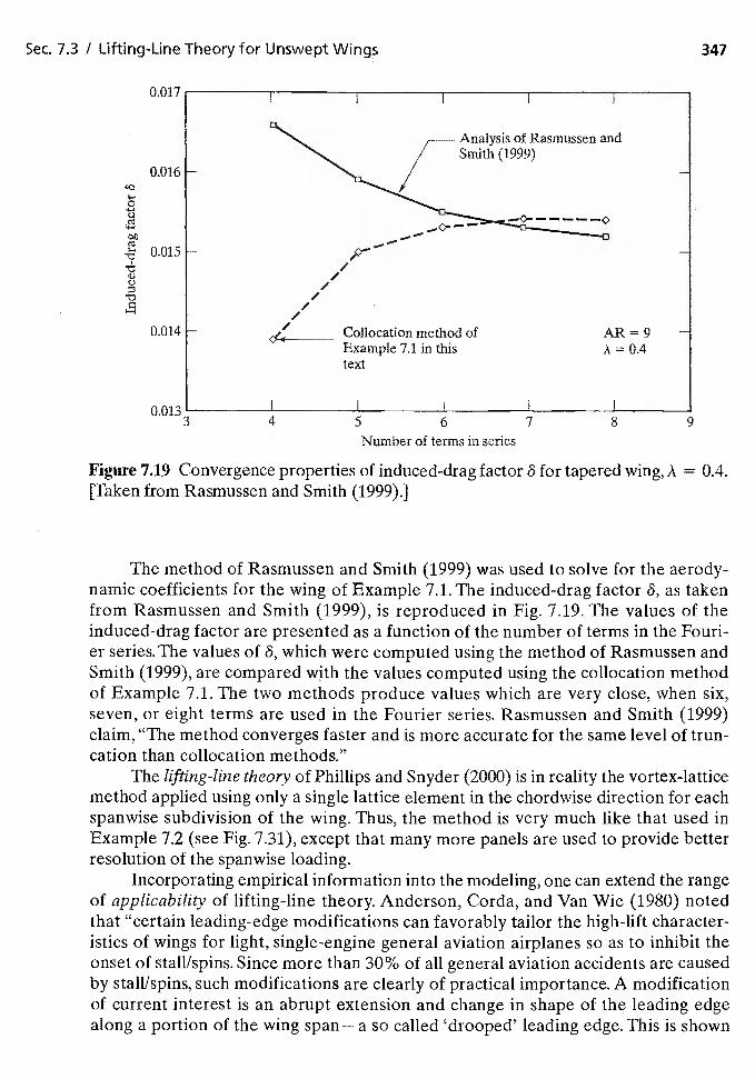
Sec. 7.3 I Lifting-Line Theory for Unswept Wings 347
0,017
0.016 —
0U
:1
0.015
0.014 —
0.013 I
3 4 6 8 9
Number of terms in series
Figure 7.19 Convergence properties of induced-drag factor 8 for tapered wing, A = 0.4.[Taken from Rasmussen and Smith (1999).]
The method of Rasmussen and Smith (1999) was used to solve for the aerody-namic coefficients for the wing of Example 7.1. The induced-drag factor 8, as takenfrom Rasmussen and Smith (1999), is reproduced in Fig. 7.19. The values of theinduced-drag factor are presented as a function of the number of terms in the Fouri-er series. The values of 6, which were computed using the method of Rasmussen andSmith (1999), are compared with the values computed using the collocation methodof Example 7.1. The two methods produce values which are very close, when six,seven, or eight terms are used in the Fourier series. Rasmussen and Smith (1999)claim, "The method converges faster and is more accurate for the same level of trun-cation than collocation methods."
The lifting-line theory of Phillips and Snyder (2000) is in reality the vortex-latticemethod applied using only a single lattice element in the chordwise direction for eachspanwise subdivision of the wing. Thus, the method is very much like that used inExample 7.2 (see Fig. 7.31), except that many more panels are used to provide betterresolution of the spanwise loading.
Incorporating empirical information into the modeling, one can extend the rangeof applicability of lifting-line theory. Anderson, Corda, and Van Wie (1980) notedthat "certain leading-edge modifications can favorably tailor the high-lift character-istics of wings for light, single-engine general aviation airplanes so as to inhibit theonset of stall/spins. Since more than 30% of all general aviation accidents are causedby stall/spins, such modifications are clearly of practical importance. A modificationof current interest is an abrupt extension and change in shape of the leading edgealong a portion of the wing span — a so called 'drooped' leading edge. This is shown
— .-7---///
//Collocation method ofExample 7.1 in thistext
AR = 9A = 0.4
5 7
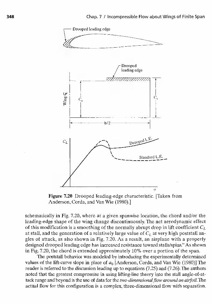
348 Chap. 7 / Incompressible Flow about Wings of Finite Span
Drooped leading edge
Droopedleading edge
Cr II
Figure 7.20 Drooped leading-edge characteristic. [Taken fromAnderson, Corda, and Van Wie (1980).]
schematically in Fig. 7.20, where at a given spanwise location, the chord and/or theleading-edge shape of the wing change discontinuously. The net aerodynamic effectof this modification is a smoothing of the normally abrupt drop in lift coefficient CLat stall, and the generation of a relatively large value of CL at very high poststall an-gles of attack, as also shown in Fig. 7.20. As a result, an airplane with a properlydesigned drooped leading edge has increased resistance toward stalls/spins." As shownin Fig. 7.20, the chord is extended approximately 10% over a portion of the span.
The poststall behavior was modeled by introducing the experimentally determinedvalues of the lift-curve slope in place of a0 [Anderson, Corda, and Van Wie (1980)] Thereader is referred to the discussion leading up to equations (7.25) and (7.26).The authorsnoted that the greatest compromise in using lifting-line theory into the stall angle-of-at-tack range and beyond is the use of data for the two-dimensional flow around an airfoil.Theactual flow for this configuration is a complex, three-dimensional flow with separation.
CL
Standard L.E.
a
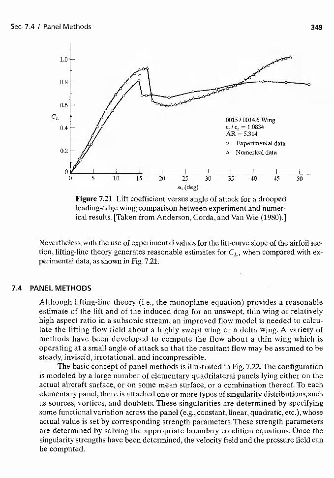
Sec. 7.4 / Panel Methods 349
CL
a, (deg)
Figure 7.21 Lift coefficient versus angle of attack for a droopedleading-edge wing; comparison between experiment andical results. [Taken from Anderson, Corda, and Van Wie (1980).]
Nevertheless, with the use of experimental values for the lift-curve slope of the airfoil sec-tion, lifting-line theory generates reasonable estimates for CL, when compared with ex-perimental data, as shown in Fig. 7.21.
7.4 PANEL METHODS
Although lifting-line theory (i.e., the monoplane equation) provides a reasonableestimate of the lift and of the induced drag for an unswept, thin wing of relativelyhigh aspect ratio in a subsonic stream, an improved flow model is needed to calcu-late the lifting flow field about a highly swept wing or a delta wing. A variety ofmethods have been developed to compute the flow about a thin wing which isoperating at a small angle of attack so that the resultant flow may be assumed to besteady, inviscid, irrotational, and incompressible.
The basic concept of panel methods is illustrated in Fig. 7.22. The configurationis modeled by a large number of elementary quadrilateral panels lying either on theactual aircraft surface, or on some mean surface, or a combination thereof. To eachelementary panel, there is attached one or more types of singularity distributions, suchas sources, vortices, and doublets. These singularities are determined by specifyingsome functional variation across the panel (e.g., constant, linear, quadratic, etc.), whoseactual value is set by corresponding strength parameters. These strength parametersare determined by solving the appropriate boundary condition equations. Once thesingularity strengths have been determined, the velocity field and the pressure field canbe computed.
1.0
0.8
0.6
c14
00 5
0015 / 0014.6 Wing1.0834
AR = 5.314
o Experimental dataix Numerical data
10 15 20 25 30 35 40 45
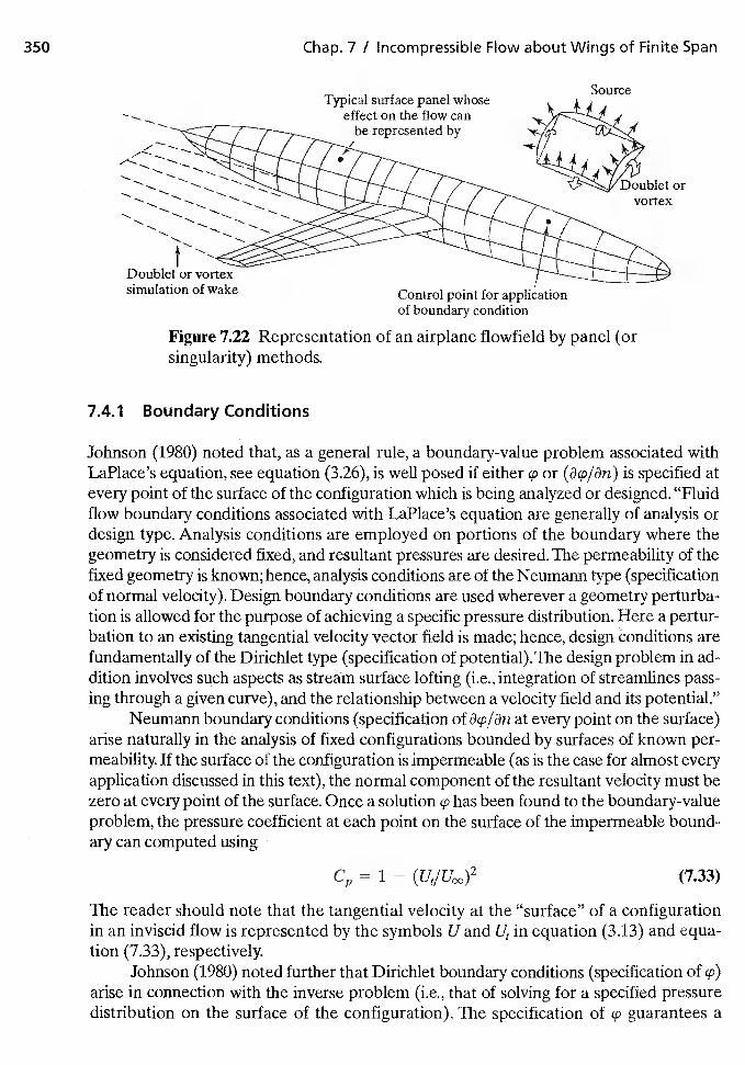
350 Chap. 7 I Incompressible Flow about Wings of Finfte Span
or
Figure 722 Representation of an airplane flowfield by panel (orsingularity) methods.
7.4.1 Boundary Conditions
Johnson (1980) noted that, as a general rule, a boundary-value problem associated withLaPlace's equation, see equation (3.26), is well posed if either q' or (acp/an) is specified atevery point of the surface of the configuration which is being analyzed or designed. "Fluidflow boundary conditions associated with LaPlace's equation are generally of analysis ordesign type. Analysis conditions are employed on portions of the boundary where thegeometry is considered fixed, and resultant pressures are desired. The permeability of thefixed geometry is known; hence, analysis conditions are of the Neumann type (specificationof normal velocity). Design boundary conditions are used wherever a geometry perturba-tion is allowed for the purpose of achieving a specific pressure distribution. Here a pertur-bation to an existing tangential velocity vector field is made; hence, design conditions arefundamentally of the Dirichiet type (specification of potential).The design problem in ad-dition involves such aspects as stream surface lofting (i.e., integration of streamlines pass-ing through a given curve), and the relationship between a velocity field and its potential."
Neumann boundary conditions (specification of at every point on the surface)arise naturally in the analysis of fixed configurations bounded by surfaces of known per-meability. If the surface of the configuration is impermeable (as is the case for almost everyapplication discussed in this text), the normal component of the resultant velocity must bezero at every point of the surface. Once a solution has been found to the boundary-valueproblem, the pressure coefficient at each point on the surface of the impermeable bound-ary can computed using
= 1 (733)
The reader should note that the tangential velocity at the "surface" of a configurationin an inviscid flow is represented by the symbols U and in equation (3.13) and equa-tion (7.33), respectively.
Johnson (1980) noted further that Dirichlet boundary conditions (specification of q')arise in connection with the inverse problem (i.e., that of solving for a specified pressuredistribution on the surface of the configuration). The specification of cp guarantees a
Typical surface panel whoseeffect on the flow can
be represented by
Source
Doublet or vortexsimulation of wake Control point for application
of boundary condition
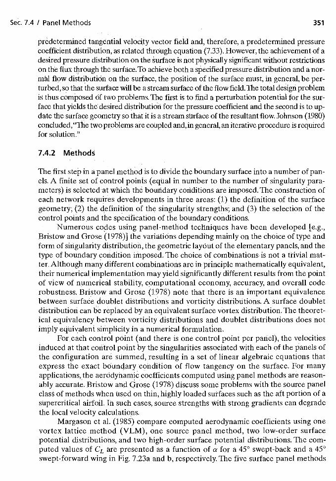
Sec. 7.4 / Panel Methods 351
predetermined tangential velocity vector field and, therefore, a predetermined pressurecoefficient distribution, as related through equation (7.33). However, the achievement of adesired pressure distribution on the surface is not physically signfficant without restrictionson the flux through the surface.To achieve both a specified pressure distribution and a nor-mM flow distributiOn on the surface, the position of the surface must, in general, be per-turbed, so that the surface will be a stream surface of the flow The total design problem
thus composed Of two problems. The first is to find a perturbation potential for the sur-face that yields the desired distribution for the pressure coefficient and the second is to up-date the surface geonietry so that it is a stream surface of the resultant flow. Johnson (1980)concluded, "The two problems are coupled and, in general, an iterative procedure is requiredfor solution."
7.4.2 Methods
The first step in a panel method is to divide the boundary surface into a number of pan-els. A finite set of control points (equal in number to the number of singularity para-meters) is selected at which the boulidary conditions are imposed. The construction ofeach network requires developments in three areas: (1) the definition of the surfacegeometry; (2) the definition of the singularity strengths; and (3) the selection of thecontrol points and the specification of the boundary conditions.
Numerous codes using panel-method techniques have been developed [e.g.,Bristow and Grose (1978)] the variations depending mainly on the choice of type andform of singularity distribution, the geOmetric layout of the elementary panels, and thetype of boundary condition imposed. The choice of combinations is not a trivial mat-ter. Although many different combinations are in principle mathematically equivalent,their numerical implementation may yield significantly different results from the pointof view of numerical stability, computational economy, accuracy, and overall coderobustness. Bristow and Grose (1978) note that there is an important equivalencebetween surface doublet distributions and vorticity distributions. A surface doubletdistribution can bè•ràplaced by an equivalent surface vortex distribution. The theoret-ical equivalency between vorticity distributions and doublet distributions does notimply e 4uivalent simplicity in a numerical
For.each control point (and there is one control point per panel), the velocitiesinduced at that control point by the singularities associated with each of the panels ofthe configuration summed, resulting in a set of linear algebraic equations thatexpress the exact condition of flow tangency on the surface. For manyapplications, the aerodynamic coefficients computed using panel methods are reason-ably accurate. Bristow and Grose (1978) discuss some problems with the source panelclass of methods when Used on thin, highly loaded surfaces such as the aft portion of asupercritical airfoil. In such cases, source strengths with strong gradients can degradethe local velocity calculations.
Margason et al. (1985) compare computed aerodynamic coefficients using onevortex lattice method (VLM), one source panel method, two low-order surfacepotential distributions, and two high-order surface potential distributions. The com-puted values of CL are presented as a function of a for a 45° swept-back and a 45°swept-forward wing in Fig. 7.23a and b, respectively. The five surface panel methods
352 Chap. 7 / Incompressible Flow about Wings of Finite Span
CL
0 Data
. Vortex lattice method
— - — - Source panel method
(a)
Figure 7.23 Comparison of the lift coefficient as a function ofangle of attack: (a) 450, 64A010 section, AR = 3.0,A 0.5, aft swept wing. [From Margason et al. (1985).]
consistently overpredict the experimental data with little difference between the liftcoefficients predicted by the various surface panel methods. As Margason et al. (1985)note, "The VLM predicts the experimental data very well, due to the fact that vortexlattice methOds neglect both thickness and viscosity effects. For most cases, the effectof viscosity offsets the effect of thickness, fortuitously yielding good agreementbetween the VLM and experiment."
7.5 VORTEX LA111CE METHOD
The vortex lattice method is the simplest of the methods reviewed by Margason, et al.(1985). The VLM represents the wing as a surface on which a grid of horseshoe vorticesis superimposed. The velocities induced by each horseshoe vortex at a specified controlpoint are calculated using the law of Biot-Savart.A summation is performed for all con-trol points on the wing to produce a set of linear algebraic equations for the horseshoe
Surface potential distributions0.6
a, deg
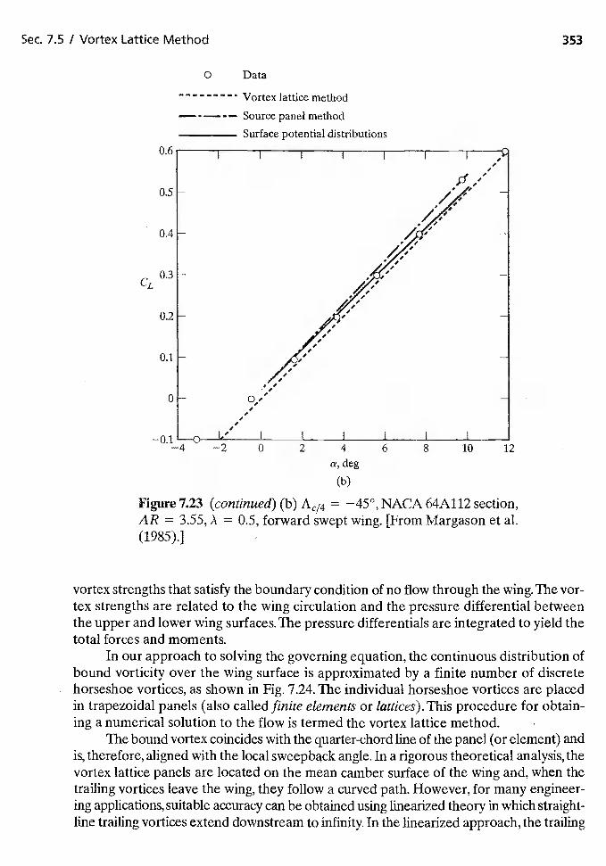
Sec. 7.5 / Vortex Lattice Method 353
0 Data
- Vortex lattice method— - — - — Source panel method
Surface potential distributions
0.6
0.5
0,4 -
0.3 -
0.2 -
0.1
0-
—2 0 2 4
a, deg
(b)
Figure 7.23 (continued) (b) = —45°, NACA 64A112 section,AR = 3.55, A = 0.5, forward swept wing. [From Margason et al.(1985).]
vortex strengths that satisfy the boundary condition of no flow through the wing. The vor-tex strengths are related to the wing circulation and the pressure differential betweenthe upper and lower wing surfaces. The pressure differentials are integrated to yield thetotal forces and moments.
In our approach to solving the governing equation, the continuous distribution ofbound vorticity over the wing surface is approximated by a finite number of discretehorseshoe vortices, as shown in Fig. 7.24. The individual horseshoe vortices are placedin trapezoidal panels (also called finite elements or lattices). This procedure for obtain-ing a numerical solution to the flow is termed the vortex lattice method.
The bound vortex coincides with the quarter-chord line of the panel (or element) andis, therefore, aligned with the local sweepback angle. In a rigorous theoretical analysis, thevortex lattice panels are located on the mean camber surface of the wing and, when thetrailing vortices leave the wing, they follow a curved path. However, for many engineer-ing applications, suitable accuracy can be obtained using linearized theory inwhich straight-line trailing vortices extend downstream to infinity In the linearized approach, the trailing
I I I I I I
I 1 I
6 8 10 12
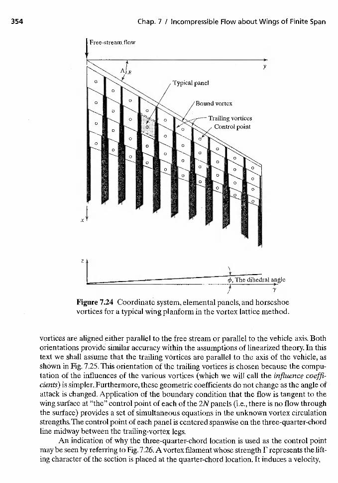
354 Chap. 7 / Incompressible Flow about Wings of Finite Span
t____The dihedral angle
I 7
Figure 7.24 Coordinate system, elemental panels, and horseshoevortices for a typical wing planform in the vortex lattice method.
vortices are aligned either parallel to the free stream or parallel to the vehicle axis. Bothorientations provide similar accuracy within the assumptions of linearized theory. In thistext we shall assume that the trailing vortices are parallel to the axis of the vehicle, asshown in Fig. 7.25. This orientation of the trailing vortices is chosen because the compu-tation of the influences of the various vortices (which we will call the influence coeffi-cients) is simpler. Furthermore, these geometric coefficients do not change as the angle ofattack is changed. Application of the boundary condition that the flow is tangent to thewing surface at "the" control point of each of the 2N panels (i.e., there is no flow throughthe surface) provides a set of simultaneous equations in the unknown vortex circulationstrengths. The control point of each panel is centered spanwise on the three-quarter-chordline midway between the trailing-vortex legs.
An indication of why the three-quarter-chord location is used as the control pointmay be seen by referring to Fig. 7.26. A vortex filament whose strength F represents the lift-ing character of the section is placed at the quarter-chord location. It induces a velocity,
Free-stream flow
y
Bound vortex
Control point
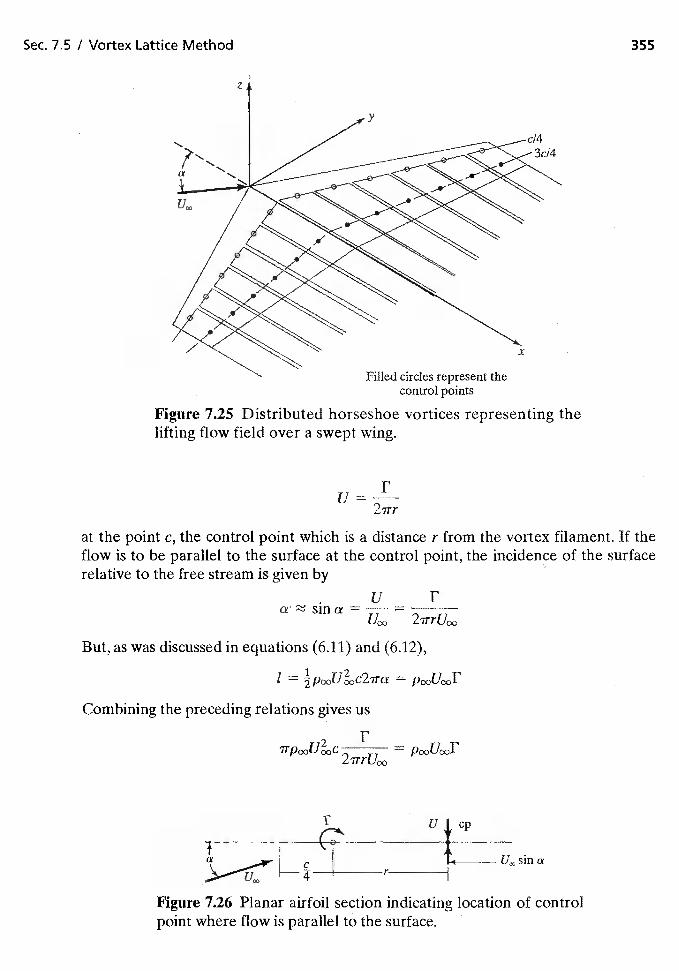
2irr
at the point c, the control point which is a distance r from the vortex filament. If theflow is to be parallel to the surface at the control point, the incidence of the surfacerelative to the free stream is given by
U Fa' Sin a =
Combining the preceding relations gives us
F=
Sec. 7.5 I Vortex Lattice Method 355
z
y
- c/4
x
Filled circles represent thecontrol points
Figure 7.25 Distributed horseshoe vortices representing thelifting flow field over a swept wing.
But, as was discussed in equations (6.11) and (6.12),
1 = =
I
Figure 7.26 Planar airfoil section indicating location of controlpoint where flow is parallel to the surface.
U,, sin a
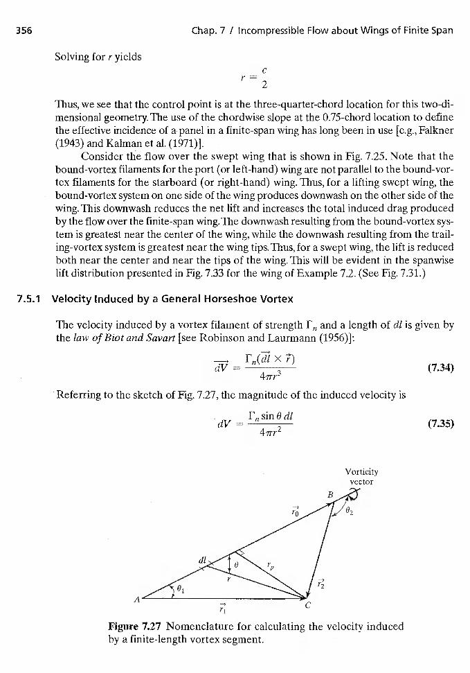
356 Chap. 7 / Incompressible Flow about Wings of Finite Span
Solving for r yieldsC
Thus, we see that the control point is at the three-quarter-chord location for this two-di-mensional geometry. The use of the chordwise slope at the 0.75-chord location to definethe effective incidence of a panel in a finite-span wing has long been in use [e.g., Falkner(1943) and Kalman et a!. (1971)].
Consider the flow over the swept wing that is shown in Fig. 7.25. Note that thebound-vortex filaments for the port (or left-hand) wing are not parallel to the bound-vor-tex filaments for the starboard (or right-hand) wing. Thus, for a lifting swept wing, thebound-vortex system on one side of the wing produces downwash on the other side of thewing. This downwash reduces the net lift and increases the total induced drag producedby the flow over the finite-span wing.The downwash resulting from the bound-vortex sys-tem is greatest near the center of the wing, while the downwash resulting from the trail-ing-vortex system is greatest near the wing tips. Thus, for a swept wing, the lift is reducedboth near the center and near the tips of the wing. This will be evident in the spanwiselift distribution presented in Fig. 7.33 for the wing of Example 7.2. (See Fig. 7.31.)
7.5.1 Velocity Induced by a General Horseshoe Vortex
The velocity induced by a vortex filament of strength and a length of dl is given bythe law of Biot and Savart [see Robinson and Laurmann (1956)]:
dV—
(7.34)
Referring to the sketch of Fig. 7.27, the magnitude of the induced velocity is
F sinOdl=2
(735)4irr
Vorticityvector
A
Figure 7.27 Nomenclature for calculating the velocity inducedby a finite-length vortex segment.
B
-3r2
-3 CTi
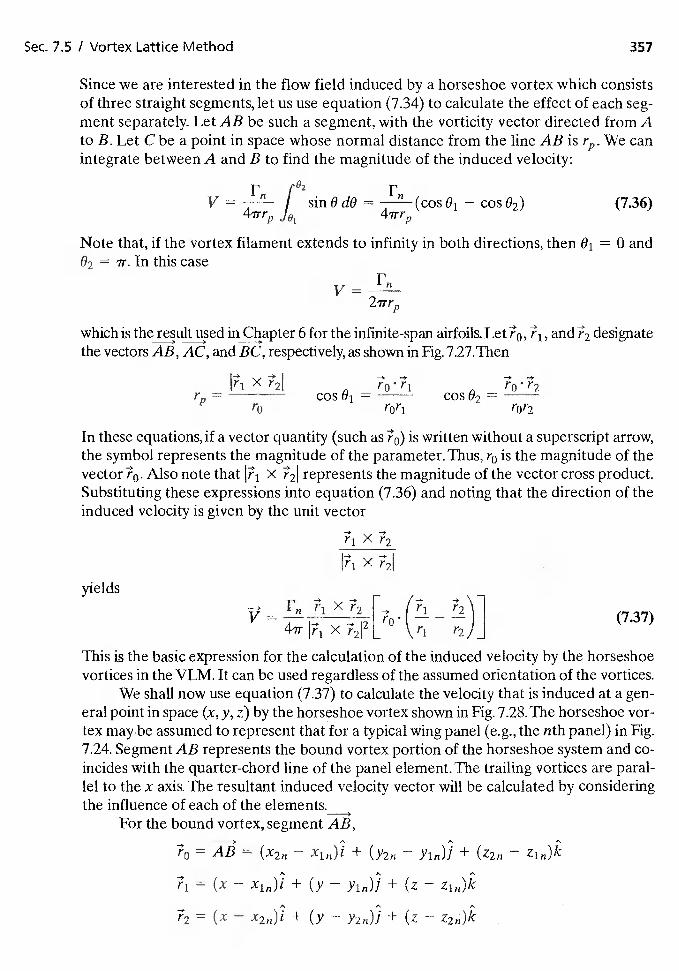
Sec. 7.5 I Vortex Lattice Method 357
Since we are interested in the flow field induced by a horseshoe vortex which consistsof three straight segments, let us use equation (7.34) to calculate the effect of each seg-ment separately. Let AB be such a segment, with the vorticity vector directed from Ato B. Let C be a point in space whose normal distance from the line AB is We canintegrate between A and B to find the magnitude of the induced velocity:
F [02
V =/ sin 0 dO =
"(cos — cos 02) (7.36)
Note that, if the vortex filament extends to infinity in both directions, then = 0 and02 = ir. In this case
Fv=
which is the result used in Chapter 6 for the infinite-span airfoils. Let and designatethe vectors AB, AC, and BC, respectively, as shown in Fig. 7.27.Then
Ti X r2(cosO1= cosO2=
r0r1 r0r2
In these equations, if a vector quantity (such asis written without a superscript arrow,the symbol represents the magnitude of the parameter. Thus, r0 is the magnitude of thevector Also note that X r21 represents the magnitude of the vector cross product.Substituting these expressions into equation (7.36) and noting that the direction of theinduced velocity is given by the unit vector
r1 X r2
yields
(7.37)IT1 X r21 L r2JJ
This is the basic expression for the calculation of the induced velocity by the horseshoevortices in the VLM. 1t can be used regardless of the assumed orientation of the vortices.
We shall now use equation (7.37) to calculate the velocity that is induced at a gen-era! point in space (x, y, z) by the horseshoe vortex shown in Fig. 7.28. The horseshoe vor-tex maybe assumed to represent that for a typical wing panel (e.g., the nth panel) in Fig.7.24. Segment AB represents the bound vortex portion of the horseshoe system and co-incides with the quarter-chord line of the panel element. The trailing vortices are paral-lel to the x axis. The resultant induced velocity vector will be calculated by consideringthe influence of each of the elements.
For the bound vortex, segment AB,
= = — + (Y2n Yin)] + (z2n —
= (x — + (y — Yin)J + (z —
(x — + (Y — Y2fl)J + (z —
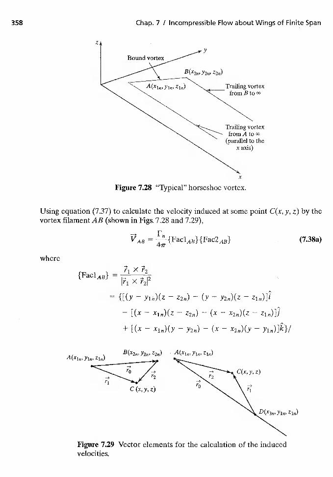
358 Chap. 7 I Incompressible Flow about Wings of Finite Span
x
Figure 7.28 "Typical" horseshoe vortex.
Using equation (7.37) to calculate the velocity induced at some point C(x, y, z) by thevortex filament AB (shown in Figs. 7.28 and 7.29),
where
FnVAB = —{FaclAB}{Fac2AB}
4ir
X T2{FaCIAB} = -, 2r1 X r2
= {{(y — — (y — Y2n)(Z —
— {(x — — — (x — —
+ {(x — Y2n) — (x — X2n)(y — Yin)]k}/
Z2fl) yin,
C(x,y,z)To
Figure 7.29 Vector elements for the calculation of the inducedvelocities.
(7.38a)
Bound vortexy
Trailing vortexfrom B to
thex axis)
C(x,y,z)
r1
Zin)
Sec. 7.5 / Vortex Lattice Method 359
{{(Y — Yin)(Z — (y — —
+ [(x — —Z2n) — (x — x2fl)(Z —
+ [(x —Xin)(y — Y2n) — (x —X2n)(y —
and
-÷ T2{FaC2AB} = r0— — r0—
= — — + (Y2n — Yin)(Y — Yin) + — —
V(x — + Yin)2 + (z — zin)2
— [(x2fl — + (Y2n —Yin)(Y —Y2n) + — —
V'(x — + (y — Y2n)2 + (z —
To calculate the velocity induced by the filament that extends from A to 00, let usfirst calculate the velocity induced by the collinear, finite-length filament that extendsfrom A to D. Since is in the direction of the vorticity vector,
= = — x3n)i
+ (Y — Yin)] + (z —
= (x — + (y — Yin)] + (z — Zin)k
as shown in Fig. 7.29. Thus, the induced velocity is
—, FVAD =
where(z — Zin)] + (Yin —y)k
{Facl D} =[(z — + (Yin Y) —
and
{Fac2AD} = — xin)TX3n —X
2IV(x — + (Y Yin)2 + (z —
+XXin
V(x — Xin)2 + (Y — Yin)2 + (z — Zin)2
Letting x3 go to 00, the first term of {Fac2AD} goes to 1.O.Theréfore, the velocity inducedby the vortex filament which extends from A to oo in a positive direction parallel to the
360 Chap. 7 I Incompressible Flow about Wings of Finite Span
x axis is given by
— J (z — Zin)J + — y)k
— + — y)2]
[1.0 +*
1 (7.38b)L — + (y — Yin)2 + (z —
Similarly, the velocity induced by the vortex filament that extends from B to oo ina positive direction parallel to the x axis is given by
f (z — + — y)k2 24ir — + — y) ]
+ X 2fl1 (7.38c)
L \/(x — + (Y — + (z —
The total velocity induced at some point (x, y, z) by the horseshoe vortex repre-senting one of the surface elements (i.e., that for the nth panel) is the sum of the com-ponents given in equation (7.38). Let the point (x, z) be the control point of the rnthpanel, which we will designate by the coordinates (xrn, The velocity induced atthe mth control point by the vortex representing the nth panel will be designated asVm,n. Examining equation (7.38), we see that
(7.39)
where the influence coefficient depends on the geometry of the nth horseshoe vor-tex and its distance from the control point of the mth panel. Since the governing equa-tion is linear, the velocities induced by the 2N vortices are added together to obtain anexpression for the total induced velocity at the rnth control point:
2N
(740)
We have 2N of these equations, one for each of the control points.
7.5.2 Application of the Boundary Conditions
Thus, it is possible to determine the resultant induced velocity at any point in space,if the strengths of the 2N horseshoe vortices are known. However, their strengths arenot known a prion.To compute the strengths of the vortices, which represent thelifting flow field of the wing, we use the boundary condition that the surface is astreamline. That is, the resultant flow is tangent to the wing at each and every controlpoint (which is located at the midspan of the three-quarter-chord line of eachelemental panel). If the flow is tangent to the wing, the component of the inducedvelocity normal to the wing at the control point balances the normal component ofthe free-stream velocity. To evaluate the induced velocity components, we mustintroduce at this point our convention that the trailing vortices are parallel to the
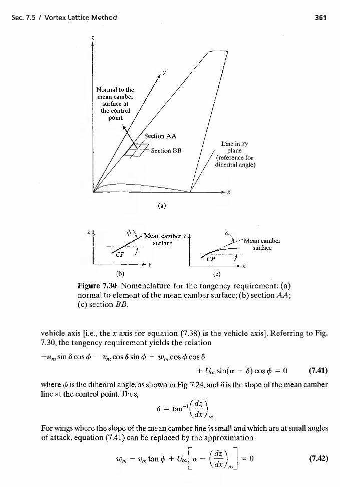
Sec. 7.5 / Vortex Lattice Method 361
z
Line in xyplane
(reference fordihedral angle)
Figure 7.30 Nomenclature for the tangency requirement: (a)normal to element of the mean camber surface; (b) section AA;(c) section BB.
vehicle axis [i.e., the x axis for equation (7.38) is the vehicle axis]. Referring to Fig.7.30, the tangency requirement yields the relation
Um S111 6 cos (1) Vm COS 6 sin 4) + Wm cos 4) cos 6
+ sin(a — 6) cos 4) = 0 (7.41)
where 4) is the dihedral angle, as shown in Fig. 7.24, and 6 is the slope of the mean camberline at the control point. Thus,
6 =dx
For wings where the slope of the mean camber line is small and which are at small anglesof attack, equation (7.41) can be replaced by the approximation
rWm — Vm tan 4) + a — -i—) = 0 (7.42)
L
(a)
Mean camber zsurface
(b)
- — Mean cambersurface
(c)
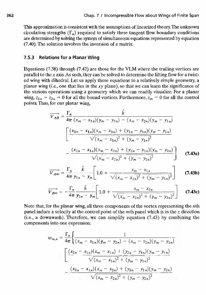
362 Chap. 7 / Incompressible Flow about Wings of Finite Span
This approximation is consistent with the assumptions of linearized theory. The unknowncirculation strengths required to satisfy these tangent flow boundary conditionsare determined by solving the systepi of simultaneous equations represented by equation(7.40). The solution involves the inversion of a matrix.
7.5.3 Relations for a Planar Wing
Equations (7.38) through (7.42) are those for the VLM where the trailing vortices areparallel to the x axis. As such, they can be solved to determine the lifting flow for a twist-ed wing withdihedral. Let us apply these equations to a relatively simple geometry, aplanar wing (i.e., one that lies in the xy plane), so that we can learn the significance ofthe various operations using a geometry which we can readily visualize. For a planarwing, = = 0 for all the bound vortices. Furthermore, Zm 0 for all the controlpoints. Thus, for our planar wing,
AB—. 4ir (Xm — Xin)(ym Y2n) — (Xm — X2n)(Ym —
— xin)(xm — + (Y2n — Yin)(Yrn — Yin)
L V'(xm — + — Yin)2
(x2n — Xin)(Xm — + (Y2n — Yin)(Ym Y2n)1— (7.43a)
— x2fl)2 + (Ym Y2n)2 J
Tl — k [ —il.u+ 7.Yin — Ym[ \/(xm — xi8)2 + (Yrn — Yin)2
F k xTI — rn fl
41TY2n YmL — + (Yrn —
Note that, for the planar wing, all three components of the vortex representing the nthpanel induce a velocity at the control point of the iiith panel which is in the z direction(i.e., a downwash). TherefOre, we can simplify equation (7.43) by combining thecomponents into one expression:
Ff1 1
41T (Xm Xin)(yrn Y2n) Yin)
— xin)(xm — + (Y2n — Yin)(Yrn — Yin)
L V(xrn — + — Yin)2
— — Xin)(Xm — + (Y2n Yin)(Yrn — Y2n)
— + —
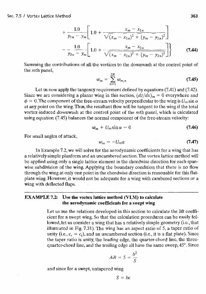
Sec. 7.5 / Vortex Lattice Method 363
+1.0
[1.0 +Xrn —
Yin YmL \/(xm — xjn)2 + (ym Yin)2
1.0 x —xj,— I 1.0 + m (7.44)
Y2n — Ym[ \/(xrn — + (Yin — Y2n)2JJ
Summing the contributions of all the vortices to the downwash at the control point ofthe mth panel,
2N
Wm = Wrn,n (7.45)n = 1
Let us now apply the tangency requirement defined by equations (7.41) and (7.42).Since we are considering a planar wing in this section, = 0 everywhere and
= 0. The component of the free-stream velocity perpendicular to the wing is sin aat any point on the wing. Thus, the resultant flow will be tangent to the wing if the totalvortex-induced downwash at the control point of the rnth panel, which is calculatedusing equation (7.45) balances the normal component of the free-stream velocity:
Wm + sin a 0 (7.46)
For small angles of attack,Wm = Uc,oa (7.47)
In Example 7.2, we will solve for the aerodynamic coefficients for a wing that hasa relatively simple planform and an uncambered section. The vortex lattice method willbe applied using only a single lattice element in the chordwise direction for each span-wise subdivision of the wing. Applying the boundary condition that there is no flowthrough the wing at only one point in the chordwise direction is reasonable for this flat-plate wing. However, it would not be adequate for a wing with cambered sections or awing with deflected flaps.
EXAMPLE 7.2: Use the vortex lattice method (VLM) to calculatethe aerodynamic coefficients for a swept wing
Let us use the relations developed in this section to calculate the lift coeffi-cient for a swept wing. So that the calculation procedures can be easily fol-lowed, let us consider a wing that has a relatively simple geometry (i.e., thatillustrated in Fig. 7.31). The wing has an aspect ratio of 5, a taper ratio ofunity (i.e., = ce), and an uncambered section (i.e., it is a flat plate). Sincethe taper ratio is unity, the leading edge, the quarter-chord line, the three-quarter-chord line, and the trailing edge all have the same sweep, 45°. Since
b2
and since for a swept, untapered wing
S bc
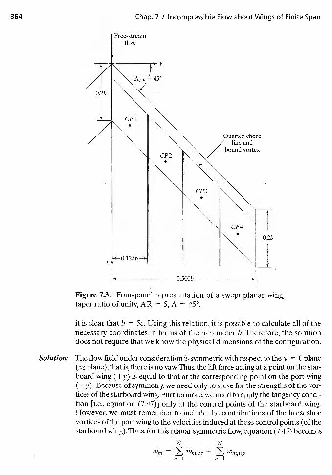
364 Chap. 7 / Incompressible Flow about Wings of Finite Span
Free-streamflow
1450
O.2b
L CP 1/bound vortex
CP2
CP3
O.2b
O.500b
Figure 7.31 Four-panel representation of a swept planar wing,taper ratio of unity, AR = 5, A = 45°.
it is clear that b = 5c. Using this relation, it is possible to calculate all of thenecessary coordinates in terms of the parameter b. Therefore, the solutiondoes not require that we know the physical dimensions of the configuration.
Solution: The flow field under consideration is symmetric with respect to the y = 0 plane(xz plane); that is, there is no the lift force acting at a point on the star-board wing (+y) is equal to that at the corresponding point on the port wing(—y). Because of symmetry, we need only to solve for the strengths of the vor-tices of the starboard wing. Furthermore, we need to apply the tangency condi-tion [i.e., equation (7.47)] only at the control points of the starboard wing.However, we must remember to include the contributions of the horseshoevortices of the port wing to the velocities induced at these control points (of thestarboard wing).Thus, for this planar symmetric flow, equation (7.45) becomes
N N
Wm = Wmns + Wm,npn1
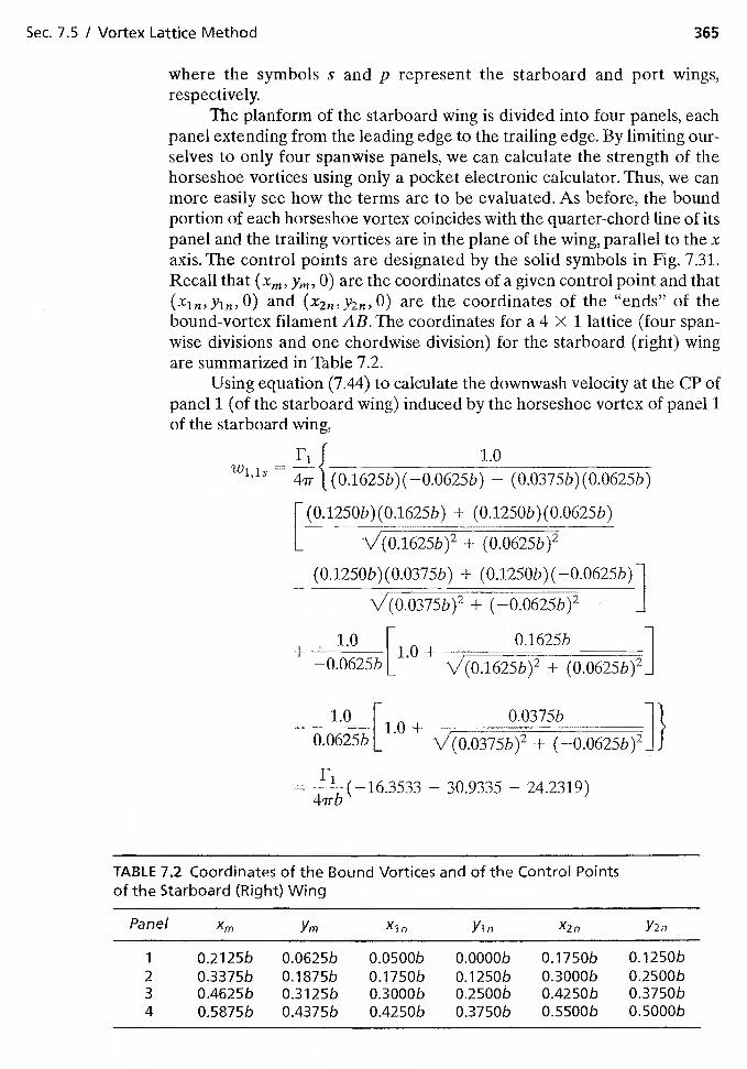
Sec. 7.5 I Vortex Lathce Method 365
where the symbols s and p represent the starboard and port wings,respectively.
The planform of the starboard wing is divided into four panels, eachpanel extending from the leading edge to the trailing edge. By limiting our-selves to only four spanwise panels, we can calculate the strength of thehorseshoe vortices using only a pocket electronic calculator. Thus, we canmore easily see how the terms are to be evaluated. As before, the boundportion of each horseshoe vortex coincides with the quarter-chord line of itspanel and the trailing vortices are in the plane of the wing, parallel to the xaxis. The control points are designated by the solid symbols in Fig. 7.31.Recall that (Xm, 0) are the coordinates of a given control point and that
and (x2fl,y2fl,O) are the coordinates of the "ends" of thebound-vortex filament AB. The coordinates for a 4 X 1 lattice (four span-wise divisions and one chordwise division) for the starboard (right) wingare summarized in Table 7.2.
Using equation (7.44) to calculate the downwash velocity at the CP ofpanel 1 (of the starboard wing) induced by the horseshoe vortex of panel 1of the starboard wing,
1.0w1,1s
— — (0.0375b)(0.0625b)
[(0.1250b)(0.1625b) + (0.1250b)(0.0625b)
L V(0.1625b)2 + (O.0625b)2
(0.1250b)(0.0375b) + (0.1250b)(—0.0625b)
V(0.0375b)2 + (—0.0625b)2
1.0 r 0.1625b_I1.0+L \/(0.1625b)2 + (0.0625b)2
1.0 [ 0.0375b
—O.O625b[L0 + V(0.0375b)2 + (—O.0625b)2
=16.3533 — 30.9335 — 24.2319)
TABLE 7.2 Coordinates of the Bound Vortices and of the Control Pointsof the Starboard (Right) Wing
Panel Xm Ym Yin Y2n
1 0.2125b O.0625b O.0500b O.0000b 0.1750b 0.1250b2 O.3375b O.1875b O.1750b 0.1250b 0.3000b O.2500b3 O.4625b O.3125b O.3000b 0.2500b 0.4250b O.3750b4 O.5875b O.4375b 0.4250b 0.37 SOb O.S500b 0.5000b
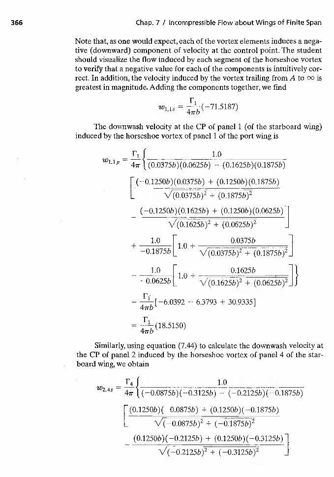
366 Chap. 7 / Incompressib'e Flow about Wings of Finite Span
Note that, as one would expect, each of the vortex elements induces a nega-tive (downward) component of velocity at the control point. The studentshould visualize the flow induced by each segment of the horseshoe vortexto verify that a negative value for each of the components is intuitively cor-rect. In addition, the velocity induced by the vortex trailing from A to isgreatest in magnitude. Adding the components together, we find
w1,1s=
The downwash velocity at the CP of panel 1 (of the starboard wing)induced by the horseshoe vortex of panel 1 of the port wing is
tow1,1p
— — (O.1625b)(0.1875b)
[(—o.l2sob)(o.o3-15b) + (0.1250b)(0.1875b)
[ \/(O.0375b)2 + (0.1875b)2
— (—0.1250b)(O.1625b) + (0.1250b)(0.0625b)
V(0.1625b)2 + (O.0625b)2
1.0 r 0.0375b+ 11.0+
—O.1875b L V(o.o375b)2 + (0.1875b)2
1.0 r O,1625b
— —0.0625b L'° + V(0.1625b)2 + (O.0625b)2
F1= —[—6.0392 — 6.3793 + 30.9335]
47th
Similarly, using equation (7.44) to calculate the downwash velocity atthe CP of panel 2 induced by the horseshoe vortex of panel 4 of the star-board wing, we obtain
to— 4 l(0.0875b)(0.3125b) — (—0.2125b)(—0.1875b)
[(0.12501,) (—0.0875b) + (0.1250b) ( —0.1875b)
L V(—0.0875b)2 + (—0.1875b)2
— (0.1250b)(—0.2125b) + (0.1250b)(—0.3125b)
V(_o.2125b)2 + (—0.3125b)2
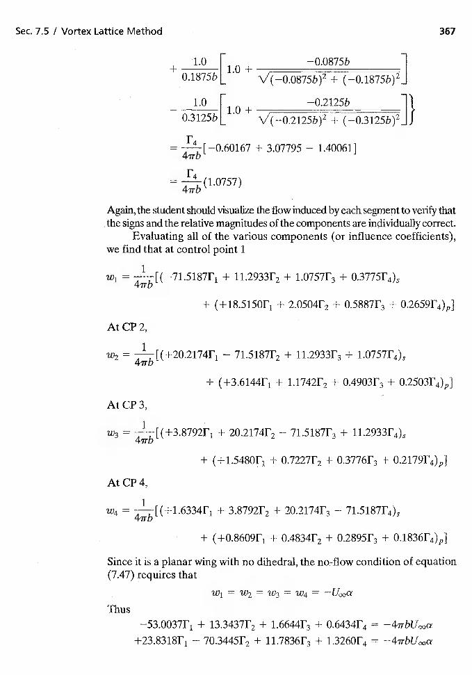
Sec. 7.5 I Vortex Lattice Method 367
'1.0 r —0.0875b
+ + V(—0.o875b)2 + (—0.1875b)2
1.0 [ —0.2125b— 11.0+
O.3125bL \/(_0.2125b)2 + (—0.3125b)2
T4—[—0.60167 + 3.07795 — 1.40061]4irb
F4—(1.0757)4'irb
Again, the student should visualize the flow induced by each segment to verify thatthe signs and the relative magnitudes of the components are individually correct.
Evaluating all of the various components (or influence coefficients),we find that at control point 1
Wi = 71.5187F1 + 11.2933F2 + 1.07571'3 + 0.3775F4)S
+ (-f-18.515OF1 + 2.0504F2 + 0.5887F3 +
At CP 2,
= — 71.5187F2 + 11.2933F3 +
+ + 1.1742F2 + o.4903F3 +
At CP 3,
+ 20.2174F2 — 71.5187F3 +
+ (+l.s4Sor'1 + 0.7227F2 + 0.37761'3 +
At CP 4,
= + 3.8792F2 + 20.2174F3 —
+ + 0.48341'2 + 0.28951'3 +
Since it is a planar wing with no dihedral, the no-flow condition of equation(7.47) requires that
Thus—53.oo37r1 + 13.34371'2 + 1.6644F3 + 0.6434F4 =
— 70.34451'2 + 11.78361'3 + 1.3260F4 =
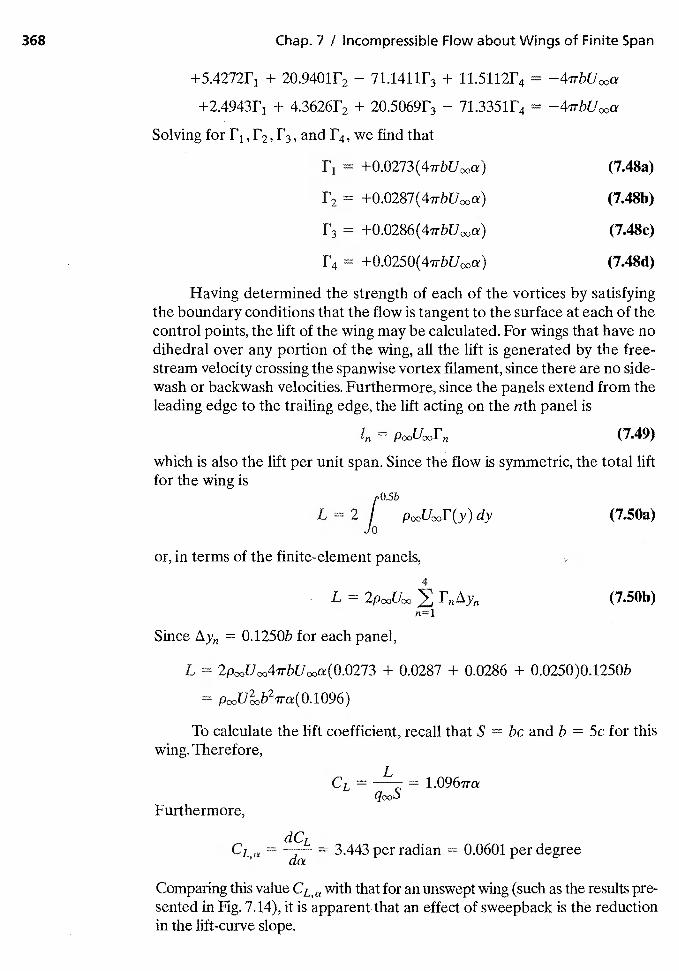
368 Chap. 7 / Incompressible Flow about Wings of Finite Span
+5.4272F1 + 2o.94o1r2 — 71.1411F3 + n.5112r4
+2.4943r1 + 4.3626f'2 + 20.5069173 — 71.3351174
Solving for 173, and 174, we find that
= (7.48a)
"2 (7.48b)
173 = (7.48c)
174 = (7.48d)
Having determined the strength of each of the vortices by satisfyingthe boundary conditions that the flow is tangent to the surface at each of thecontrol points, the lift of the wing may be calculated. For wings that have nodihedral over any portion of the wing, all the lift is generated by the free-stream velocity crossing the spanwise vortex filament, since there are no side-wash or backwash velocities. Furthermore, since the panels extend from theleading edge to the trailing edge, the lift acting on the nth panel is
= (7.49)
which is also the lift per unit span. Since the flow is symmetric, the total liftfor the wing is
L = 2 J dy (7.50a)0
or, in terms of the finite-element panels,
4
L = (7.50b)
Since = 0.1250b for each panel,
L + 0.0287 + 0.0286 + 0.0250)0.1250b
To calculate the lift coefficient, recall that S = bc and b = Sc for thiswing. Therefore,
CL = —f-- = 1.0961Ta
Furthermore,
dCLCL,a = = 3.443 per radian 0.0601 per degree
Comparing this value CL, a with that for an unswept wing (such as the results pre-sented in Fig. 7.14), it is apparent that an effect of sweephack is the reductionin the lift-curve slope.

2F— —
av
Sec. 7.5 / Vortex Lattice Method 369
o Data from Weber and Brebner (1958)
Inviscid solutiOn using VLM for 4)< 1 lattice
CL
0 2 4 6 8 10 12
Figure 7.32 Comparison of the theoretical and the experimentallift coefficients for the swept wing of Fig. 7.31 in a subsonic stream.
The theoretical lift curve generated using the VLM is compared inFig.7.32 with experimental results reported by Weber and Brebner (1958). Theexperimentally determined values of the lift coefficient are for a wing of con-stant chord and of constant section, which was swept 45° and which had anaspect ratio of 5. The theoretical lift coefficients are in good agreement withthe experimental values.
Since the lift per unit span is given by equation (7.49), the section lift coefficient for thenth panel is
When the panels extend from the leading edge to the trailing edge, such as is the casefor the 4 X 1 lattice shown in Fig. 7.31, the value of 1' given in equation (7.48) is used
(7.51)
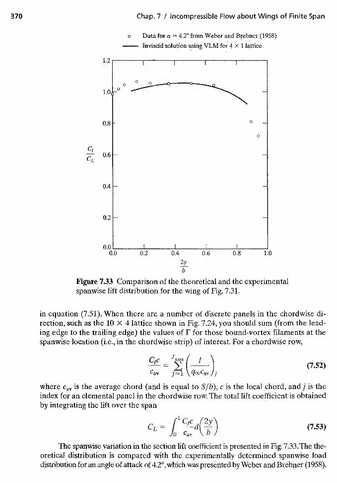
370 Chap. 7 / Incompressible Flow about Wings of Finite Span
a Data for a = 4.20 from Weber and l3rebner (1958)
Inviscid solution using VLM for 4 X 1 lattice
12
1.0
-o °
0.8- °
0
CI0.6 -
CL
0.4 -
0.2 -
0.0 I
0.0 0.2 0.4 0,6 0.8 1.0
2y
b
Figure 7.33 Comparison of the theoretical and the experimentalspanwise lift distribution for the wing of Fig. 7.31.
in equation (7.51). When there are a number of discrete panels in the chordwise di-rection, such as the 10 X 4 lattice shown in Fig. 7.24, you should sum (from the lead-ing edge to the trailing edge) the values of I' for those bound-vortex filaments at thespanwise location (i.e., in the chordwise strip) of interest. For a chordwise row,
Jmax( 1(7.52)
Cay \, Jjwhere Cay is the average chord (and is equal to S/b), c is the local chord, and j is theindex for an elemental panel in the chordwise row. The total lift coefficient is obtainedby integrating the lift over the span
CL= L (7.53)
The spanwise variation in the section lift coefficient is presented in Fig. 7.33.The the-oretical distrjbution is compared with the experimentally determined spanwise loaddistribution for anangle of attack of 4.2°, which was presented by Weber and Brebner (1958).
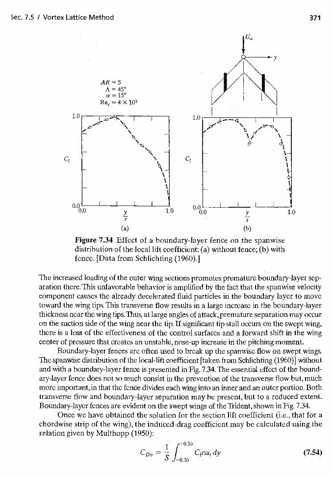
Sec. 7.5 I Vortex Lattice Method 371
+03b
k) —O.5b
y
1.0 1.0
AR =5A = 45°a 150
= 4 X
I I
C! CI
\ \\ -
(9
—
0.00.0 1.0 o.%o y 1.0
(a) (b)
Figure 7.34 Effect of a boundary-layer fence on the spanwisedistribution of the local lift coefficient: (a) without fence; (b) withfence. [Data from Schlichting (1960).]
The increased loading of the outer wing sections promotes premature boundary-layer sep-aration there, This unfavorable behavior is amplified by the fact that the spanwise velocitycomponent causes the already decelerated fluid particles in the boundary layer to movetoward the wing tips. This transverse flow results in a large increase in the boundary-layerthickness near the wing tips.Thus, at large angles of attack, premature separation may occuron the suction side of the wing near the tip. If significant tip stall occurs on the swept wing,there is a loss of the effectiveness of the control surfaces and a forward shift in the wingcenter of pressure that creates an unstable, nose-up increase in the pitching moment.
Boundary-layer fences are often used to break up the spanwise flow on swept wings.The spanwise distribution of the local-lift coefficient [taken from Schlichting (1960)] withoutand with a boundary-layer fence is presented in Fig. 7.34. The essential effect of the bound-ary-layer fence does not so much consist in the prevention of the transverse flow but, muchmore important, in that the fence divides each wing into an inner and an outer portion. Bothtransverse flow and boundary-layer separation may be present, but to a reduced extent.Boundary-layer fences are evident on the swept wings of the Trident, shown in Fig. 7.34.
Once we have obtained the solution for the section lift coefficient (i.e., that for achordwise strip of the wing), the induced-drag coefficient may be calculated using therelation given by Multhopp (1950):
dy (7.54)
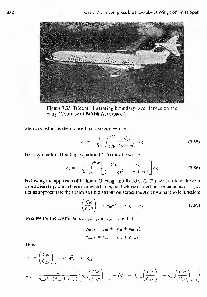
O.5bC1c C1c 11
___________ ___________
a1= [(y —
+(y +
I cic\(;;—:: I = amY!2 + + Cm
fC1c'\ 2Cm = — —
dmj( -1 {
am = d dmo(dmi + dmo)'iii
(C1c— +
\CLC
(C1c+
CLC
372 Chap. 7 I Incompressible Flow about Wings of Finite Span
Following the approach of Kalman, Giesing, and Rodden (1970), we consider the mthchordwise strip, which has a semiwidth of em and whose centerline is located at 77 Ym
Let us approximate the spanwise lift distribution across the strip by a parabolic function:
(7.57)
Figure 7.35 Trident illustrating boundary-layer fences on thewing. (Courtesy of British Aerospace.)
where a1, which is the induced incidence, given by
1 C1C
a symmetrical loading, equation (755) may be written
(7.55)
(7.56)
To solve for the coefficients am, bm, and cm, note that
Ym+i = y,71 + (em +
Yin—i = + em_i)
Thus,
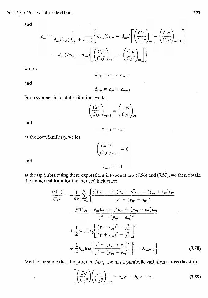
Sec. 7.5 / Vortex Lattice Method 373
and
1 1bm
= dmidmo(dmi + dmo) —
(C1c— dmj(27)m — dmi)i —
m
wheredmi em + em_i
anddmoem+em+i
For a symmetric load distribution, we let
andem_i = em
at the root. Similarly, we let
—
andem+i = 0
at the tip. Substituting these expressions into equations (7.56) and (7.57), we then obtainthe numerical form for the induced incidence:
a.(y) — 1 N JY2(Ym + em)am + y2bm + + em) Cm
CLc — 1 y2 — +
y2(ym ern)am + y2bm + em)cm
(yrn —
1
22 (y+ern) Yrn
+ iog[Y + em)]2+ 2emam} (7.58)
Y
We then assume that the product also has a parabolic variation across the strip.
= + + (7.59)
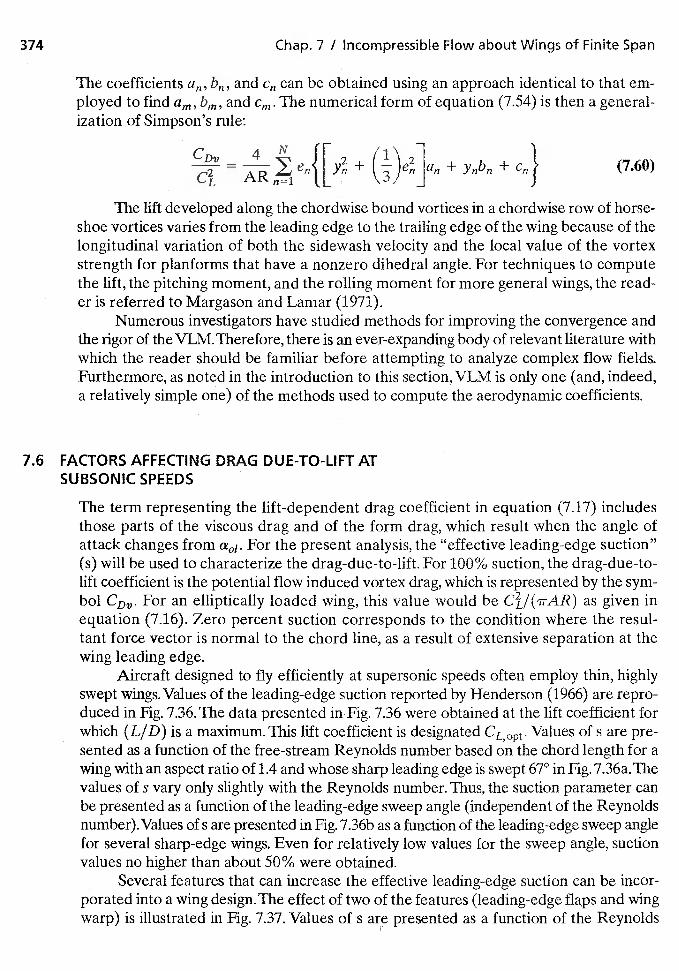
374 Chap. 7 / Incompressible Flow about Wings of Finite Span
The coefficients and can be obtained using au approach identical to that em-ployed to find am, bm, afld Cm. The numerical form of equation (7.54) is then a general-ization of Simpson's rule:
C A N rDv_ )I i'— A y,, -r
n1The lift developed along the chordwise bound vortices in a chordwise row of horse-
shoe vortices varies from the leading edge to the trailing edge of the wing because of thelongitudinal variation of both the sidewash velocity and the local value of the vortexstrength for planforms that have a nonzero dihedral angle. For techniques to computethe lift, the pitching moment, and the rolling moment for more general wings, the read-er is referred to Margason and Lamar (1971).
Numerous investigators have studied methods for improving the convergence andthe rigor of the VLM. Therefore, there is an ever-expanding body of relevant literature withwhich the reader should be familiar before attempting to analyze complex flow fields.Furthermore, as noted in the introduction to this section, VLM is only one (and, indeed,a relatively simple one) of the methods used to compute the aerodynamic coefficients.
7.6 FACTORS AFFECTING DRAG DUE-TO-LIFT ATSUBSONIC SPEEDS
The term representing the lift-dependent drag coefficient in equation (7.17) includesthose parts of the viscous drag and of the form drag, which result when the angle ofattack changes from a01. For the present analysis, the "effective leading-edge suction"(s) will be used to characterize the drag-due-to-lift. For 100% suction, the drag-due-to-lift coefficient is the potential flow induced vortex drag, which is represented by the sym-bol CDT. For an elliptically loaded wing, this value would be as given inequation (7.16). Zero percent suction corresponds to the condition where the resul-tant force vector is normal to the chord line, as a result of extensive separation at thewing leading edge.
Aircraft designed to fly efficiently at supersonic speeds often employ thin, highlyswept wings. Values of the leading-edge suction reported by Henderson (1966) are repro-duced in Fig. 7.36. The data presented inFig. 7.36 were obtained at the lift coefficient forwhich (LID) is a maximum. This lift coefficient is designated CL opt• Values of s are pre-sented as a function of the free-stream Reynolds number based on the chord length for awing with an aspect ratio of 1.4 and whose sharp leading edge is swept 67° in Fig. 7.36a. Thevalues of s vary only slightly with the Reynolds number. Thus, the suction parameter canbe presented as a function of the leading-edge sweep angle (independent of the Reynoldsnumber).Values of s are presented in Fig. 7.36b as a function of the leading-edge sweep anglefor several sharp-edge wings. Even for relatively low values for the sweep angle, suctionvalues no higher than about 50% were obtained.
Several features that can increase the effective leading-edge suction can be incor-porated into a wing design. The effect of two of the features (leading-edge flaps and wingwarp) is illustrated in Fig. 7.37. Values of s are presented as a function of the Reynolds
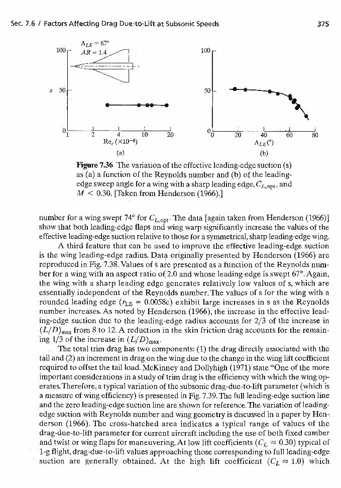
Sec. 7.6 I Factors Affecting Drag Due-to-Lift at Subsonic Speeds 375
100- 100-
•
:;(X106) ALE(°)
(a) (b)
Figure 7.36 The variation of the effective leading-edge suction (s)as (a) a function of the Reynolds number and (b) of the leading-edge sweep angle for a wing with a sharp leading edge, CL,OPt, andM < 0.30. [Taken from Henderson (1966).]
number for a wing swept 74° for The data [again taken from Henderson (1966)]show that both leading-edge flaps and wing warp significantly increase the values of theeffective leading-edge suction relative to those for a symmetrical, sharp leading-edge wing.
A third feature that can be used to improve the effective leading-edge suctionis the wing leading-edge radius. Data originally presented by Henderson (1966) arereproduced in Fig. 7.38. Values of s are presented as a function of the Reynolds num-ber for a wing with an aspect ratio of.2.0 and whose leading edge is swept 67°. Again,the wing with a sharp leading edge generates relatively low values of s, which areessentially independent of the Reynolds number, The values of s for the wing with arounded leading edge (rLE = 0.0058c) exhibit large increases in s as the Reynoldsnumber increases. As noted by Henderson (1966), the increase in the effective lead-ing-edge suction due to the leading-edge radius accounts for 2/3 of the increase in(L/D)max from 8 to 12. A reduction in the skin friction drag accounts for the remain-ing 1/3 of the increase in (L/D)max.
The total trim drag has two components: (1) the drag directly associated with thetail and (2) an increment in drag on the wing due to the change in the wing lift coefficientrequired to offset the tail load. McKinney and Dollyhigh (1971) state "One of the moreimportant considerations in a study of trim drag is the efficiency with which the wing op-erates. Therefore, a typical variation of the subsonic drag-due-to-lift parameter (which isa measure of wing efficiency) is presented in Fig. 7.39. The full leading-edge suction lineand the zero leading-edge suction line are shown for reference. The variation of leading-edge suction with Reynolds number and wing geometry is discussed in a paper by Hen-.derson (1966). The cross-hatched area indicates a typical range of values of thedrag-due-to-lift parameter for current aircraft including the use of both fixed camberand twist or wing flaps for maneuvering. At low lift coefficients (CL 0.30) typical of1-g flight, drag-due-to-lift values approaching those corresponding to full leading-edgesuction are generally obtained. At the high lift coefficient (CL 1.0) which
A 'iiAR=1.4
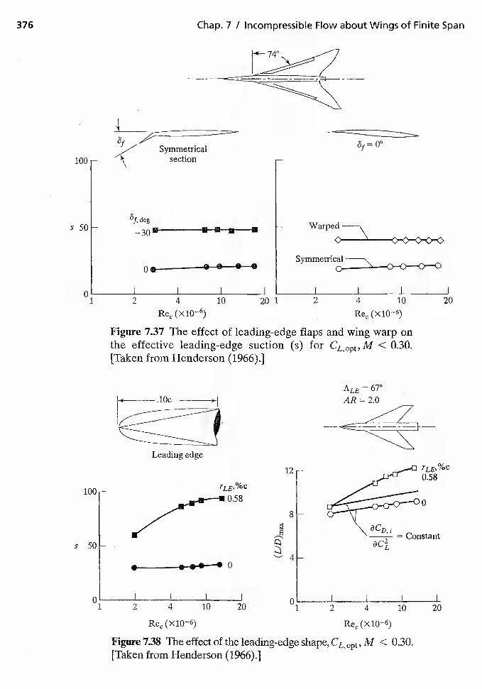
376 Chap. 7 / Incompressible Flow about Wings of Finite Span
Symmetricalsection
-
I I I I
= 00
8f,deg
0•— • S S •
100
s 50 -
Oi_- 2 4 10 20 1 2 4 10 20
(X106)
Figure 7.37 The effect of leading-edge flaps and wing warp onthe effective leading-edge suction (s) for CL0I,t,M < 0.30.[Taken from Henderson (1966).]
12
100 - rLE,%c0.58
8
s 50 -
C 01 2 4 10 20 1 2 4 10 20
(X10—6)
Figure 7.38 The effect of the leading-edge shape, CL <0.30.[Taken from Henderson (1966).]
A U,
AR = 2.0
Leading edge
TLE,%C0.58
3CD I= Constant
ac2L
I I I
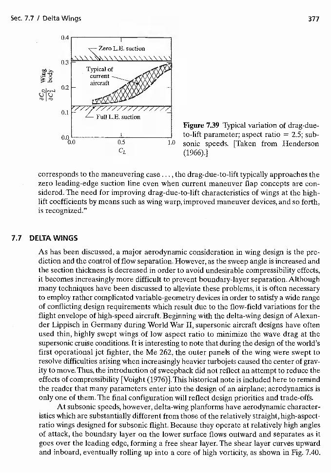
Sec. 7.7 / Defta Wings 377
0
c)c)
Figure 7.39 Typical variation of drag-due-to-lift parameter; aspect ratio = 2.5; sub-
1.0 sonic speeds. [Taken from Henderson(1966).]
corresponds to the maneuvering case ... , the drag-due-to-lift typically approaches thezero leading-edge suction line even when current maneuver flap concepts are con-sidered. The need for improving drag-due-to-lift characteristics of wings at the high-lift coefficients by means such as wing warp, improved maneuver devices, and so forth,is recognized."
7.7 DELTA WINGS
As has been discussed, a major aerodynamic consideration in wing design is the pre-diction and the control of flow separation. However, as the sweep angle is increased andthe section thickness is decreased in order to avoid undesirable compressibility effects,it becomes increasingly more difficult to prevent boundary-layer separation. Althoughmany techniques have been discussed to alleviate these problems, it is often necessaryto employ rather complicated variable-geometry devices in order to satisfy a wide rangeof conflicting design requirements which result due to the flow-field variations for theflight envelope of high-speed aircraft. Beginning with the delta-wing design of Alexan-der Lippisch in Germany during World War II, supersonic aircraft designs have oftenused thin, highly swept wings of low aspect ratio to minimize the wave drag at thesupersonic cruise conditions. It is interesting to note that during the design of the world'sfirst operational jet fighter, the Me 262, the outer panels of the wing were swept toresolve difficulties arising when increasingly heavier turbojets caused the center of grav-ity to move. Thus, the introduction of sweepback did not reflect an attempt to reduce theeffects of compressibility [Voight (1976)}.This historical note is included here to remindthe reader that many parameters enter into the design of an airplane; aerodynamics isonly one of them. The final configuration will reflect design priorities and trade-offs.
At subsonic speeds, however, delta-wing planforms have aerodynamic character-istics which are substantially different from those of the relatively straight, high-aspect-ratio wings designed for subsonic flight. Because they operate at relatively high anglesof attack, the boundary layer on the lower surface flows outward and separates as itgoes over the leading edge, forming a free shear layer. The shear layer curves upwardand inboard, eventually rolling up into a core of high vorticity, as shown in Fig. 7.40.
0.3
0.2
0,1
0.5
CL
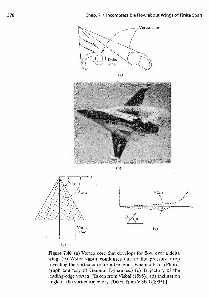
378 Chap. 7 / Incompressible Flow about Wings of Finite Span
(c)
y
(d)
Figure 7.40 (a) Vortex core that .develops for flow over a deltawing. (b) Water vapor condenses due to the pressure droprevealing the vortex core for a General Dynamic F-16. (Photo-graph courtesy of General Dynamics.) (c) Trajectory of theleading-edge vortex. [Taken from Visbal (1995).] (d) Inclinationangle of the vortex trajectory. [Taken from Visbal (1995).]
x
(a)
(b)
aCoreI
1I
Vortexcore
U7<a
x
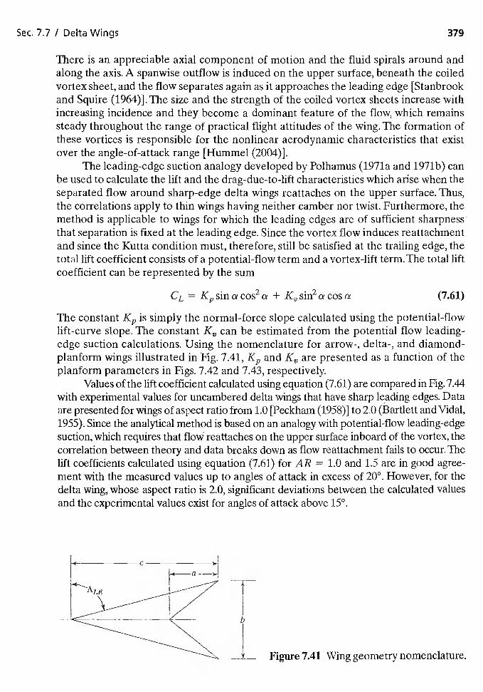
Sec. 7.7 I Delta Wings 379
There is an appreciable axial component of motion and the fluid spirals around andalong the axis. A spanwise outflow is induced on the upper surface, beneath the coiledvortex sheet, and the flow separates again as it approaches the leading edge [Stanbrookand Squire (1964)]. The size and the strength of the coiled vortex sheets increase withincreasing incidence and they become a dominant feature of the flow, which remainssteady throughout the range of practical flight attitudes of the wing. The formation ofthese vortices is responsible for the nonlinear aerodynamic characteristics that existover the angle-of-attack range [Hummel (2004)].
The leading-edge suction analogy developed by Poihamus (1971a and 1971b) canbe used to calculate the lift and the drag-due-to-lift characteristics which arise when theseparated flow around sharp-edge delta wings reattaches on the upper surface. Thus,the correlations apply to thin wings having neither camber nor twist. Furthermore, themethod is applicable to wings for which the leading edges are of sufficient sharpnessthat separation is fixed at the leading edge. Since the vortex flow induces reattachmentand since the Kutta condition must, therefore, still be satisfied at the trailing edge, thetotal lift coefficient consists of a potential-flow term and a vortex-lift term. The total liftcoefficient can be represented by the sum
CL = sin a cos2 a + sin2 a cos a (7.61)
The constant is simply the normal-force slope calculated using the potential-flowlift-curve slope. The constant be estimated from the potential flow leading-edge suction calculations. Using the nomenclature for arrow-, delta-, and diamond-planform wings illustrated in Fig. 7.41, and are presented as a function of theplanform parameters in Figs. 7.42 and 7.43, respectively.
Values of the lift coefficient calculated using equation (7.61) are compared in Fig. 7.44with experimental values for uncambered delta wings that have sharp leading edges. Dataare presented for wings of aspect ratio from 1.0 [Peckham (1958)] to 2.0 (Bartlett and Vidal,1955). Since the analytical method is based on an analogy with potential-flow leading-edgesuction, which requires that flow reattaches on the upper surface inboard of the vortex, thecorrelation between theory and data breaks down as flow reattachment fails to occur. Thelift coefficients calculated using equation (7.61) for AR = 1.0 and 1.5 are in good agree-ment with the measured values up to angles of attack in excess of 20°. However, for thedelta wing, whose aspect ratio is 2.0, significant deviations between the calculated valuesand the experimental values exist for angles of attack above 15°.
I Figure 7.41 Wing geometry nomenclature.
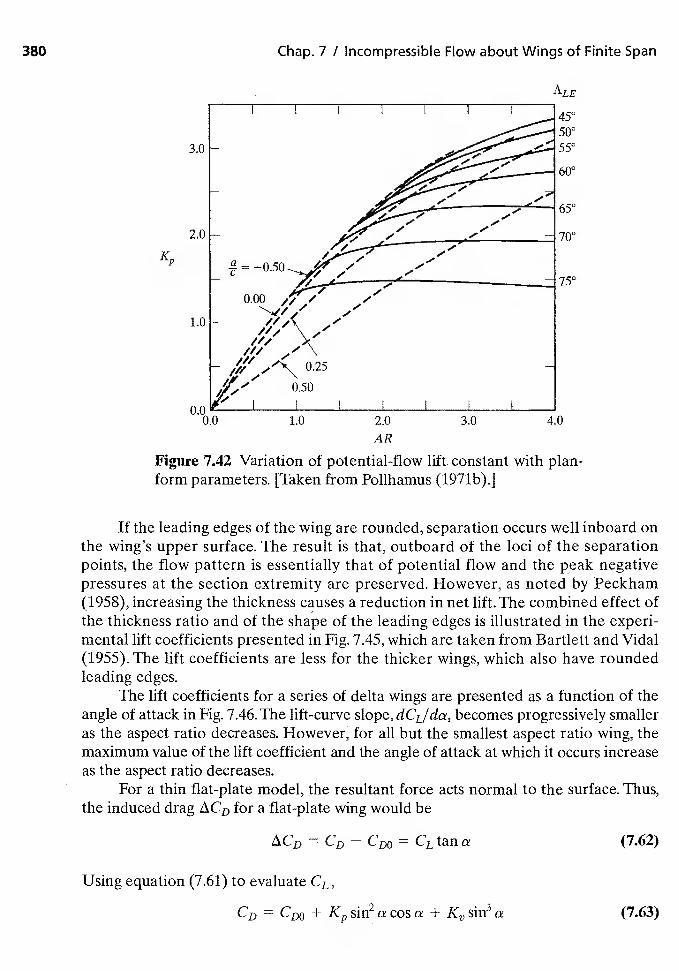
380 Chap. 7 / Incompressible Flow about Wings of Finite Span
ALE
45°500550
600
650
700
75°
1.0 2.0 3.0 4.0
AR
Figure 7.42 Variation of potential-flow lift constant with plan-form parameters. [Taken from Polihamus (1971b).]
If the leading edges of the wing are rounded, separation occurs well inboard onthe wing's upper surface, The result is that, outboard of the loci of the separationpoints, the flow pattern is essentially that of potential flow and the peak negativepressures at the section extremity are preserved. However, as noted by Peckham(1958), increasing the thickness causes a reduction in net lift. The combined effect ofthe thickness ratio and of the shape of the leading edges is illustrated in the experi-mental lift coefficients presented in Fig. 7.45, which are taken from Bartlett and Vidal(1955). The lift coefficients are less for the thicker wings, which also have roundedleading edges.
The lift coefficients for a series of delta wings are presented as a function of theangle of attack in Fig. 7,46. The lift-curve slope, dCL/da, becomes progressively smalleras the aspect ratio decreases. However, for all but the smallest aspect ratio wing, themaximum value of the lift coefficient and the angle of attack at which it occurs increaseas the aspect ratio decreases.
For a thin flat-plate model, the resultant force acts normal to the surface. Thus,the induced drag for a flat-plate wing would be
= CD = CL tan a (7.62)
Using equation (7.61) to evaluate CL,
CD = CDO + + (7.63)
0.00.0
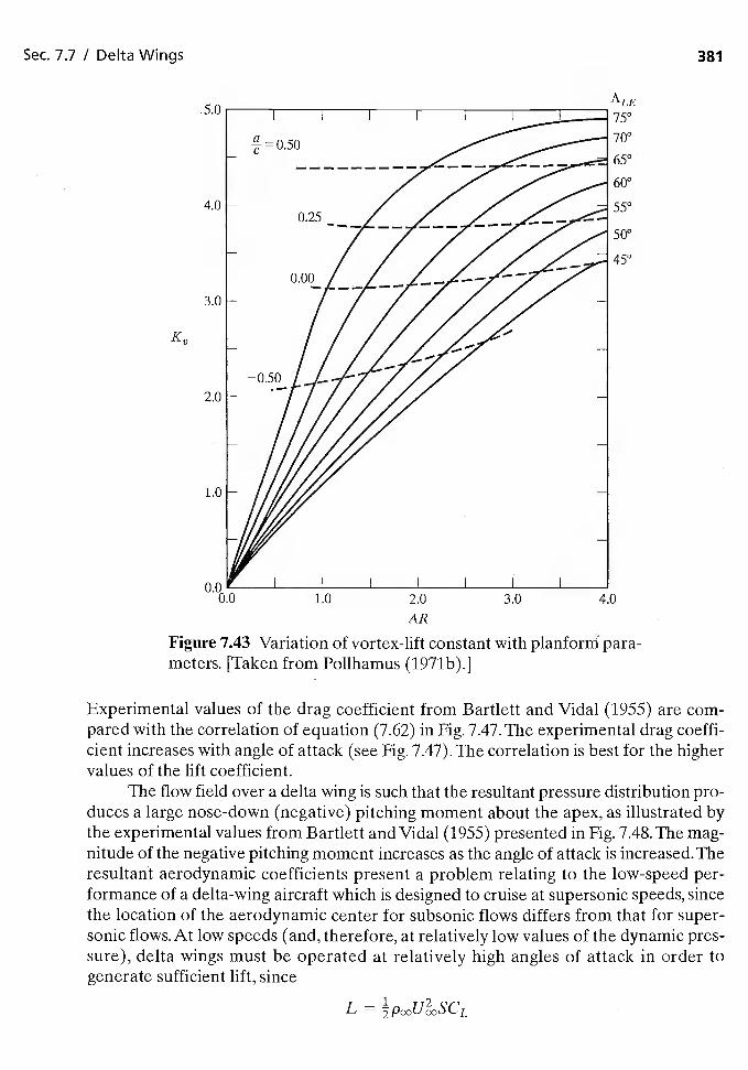
0.00.0 2.0
AR
Figure 7.43 Variation of vortex-lift constant with planforrrI para-meters. [Taken from Pollhamus (1971b).J
Experimental values of the drag coefficient from Bartlett and Vidal (1955) are com-pared with the correlation of equation (7.62) in Fig. 7.47. The experimental drag coeffi-cient increases with angle of attack (see Fig. 7.47). The correlation is best for the highervalues of the lift coefficient.
The flow field over a delta wing is such that the resultant pressure distribution pro-duces a large nose-down (negative) pitching moment about the apex, as illustrated bythe experimental values from Bartlett and Vidal (1955) presented in Fig. 7.48.The mag-nitude of the negative pitching moment increases as the angle of attack is increased.Theresultant aerodynamic coefficients present a problem relating to the low-speed per-formance of a delta-wing aircraft which is designed to cruise at supersonic speeds, sincethe location of the aerodynamic center for subsonic flows differs from that for super-sonic flows. At low speeds (and, therefore, at relatively low values of the dynamic pres-sure), delta wings must be operated at relatively high angles of attack in order togenerate sufficient lift, since
L - 2POOUOSCL
5.0
Sec. 7.7 / Delta Wings 381
ALE750
700
65°
60°
55°
50°
450
4.0
3.0
2.0
1.0
LU 3.0 4.0
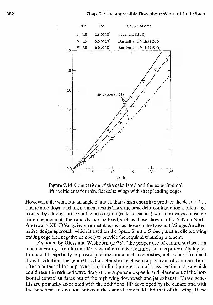
AR Source of data
0 1.0 2.6 X 10⁶ Peckham (1958)
0 1.5 6.0 X 10⁶ Bartlett and Vidal (1955)
V 2.0 6.0 X 10⁶ Bartlett and Vidal
Figure 7.44 Comparison of the calculated and the experimentallift coefficients for thin, flat delta wings with sharp leading edges.
However, if the wing is at an angle of attack that is high enough to produce the desired CL,a large nose-down pitching moment results. Thus, the basic delta configuration is often aug-mented by a lifting surface in the nose region (called a canard), which provides a nose-uptrimming moment. The canards may be fixed, such as those shown in Fig. 7.49 on NorthAmerican's XB-70 Valkyrie, or retractable, such as those on the Dassault Mirage. An alter-native design approach, which is used on the Space Shuttle Orbiter, uses a reflexed wingtrailing edge (i.e., negative camber) to provide the required trimming moment.
As noted by Gloss and Washburn (1978), "the proper use of canard surfaces ona maneuvering aircraft can offer several attractive features such as potentially highertrimmed-lift capability, improved pitching moment characteristics, and reduced trimmeddrag. In addition, the geometric characteristics of close-coupled canard configurationsoffer a potential for improved longitudinal progression of cross-sectional area whichcould result in reduced wave drag at low supersonic speeds and placement of the hor-izontal control surfaces out of the high wing downwash and jet exhaust." These bene-fits are primarily associated with the additional lift developed by the canard and withthe beneficial interaction between the canard flow field and that of the wing. These
382 Chap. 7 I Incompressible Flow about Wings of Finite Span
CL
0 5 10 15 20 25
a, deg
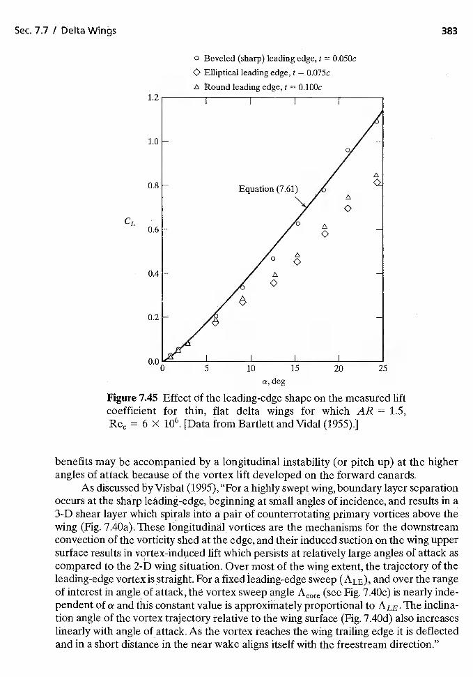
Sec. 7.7 I Delta Wings 383
CL
o Beveled (sharp) leading edge, t = O.050c
O Elliptical leading edge, t = O.075c
kound leading edge, t = O.lOOc
Figure 7.45 Effect df the leading-edge shape on the measufed liftcoefficient for thin, flat delta wings for which AR = 1.5,
= 6 x 10⁶. [Data from Bartlett and Vidal (1955).]
benefits may be accompanied by a longitudinal instability (or pitch up) at the higherangles of attack of the vortex lift developed on the forward canards.
As discussed by Visbal (1995),"For a highly swept wing, boundary layer separationoccurs at the sharp leading-edge, beginning at small angles of incidence, and results in a3-D shear layer which spirals intO a pair of counterrotating primary vortices above thewing (Fig. 7.40a). These longitudinal vortices are the mechanisms for the downstreamconvection of the vOrticity shed at the edge, and their induced suction on the wing uppersurface results in vortex-induced lift which persists at relatively large angles of attack ascompared to the 2-D wing situation. Over most of the wing extent, the trajectory of theleading-edge vortex is straight. For a fixed leading-edge sweep (ALE), and over the rangeof interest in angle of attack, the vortex sweep angle Acore (see Fig. 7.40c) is nearly inde-pendent of a and this constant value is approximately proportional to ALE. The inclina-tion angle of the vortex trajectory relative to the wing surface (Fig. 7.40d) also increaseslinearly with angle of attack. As the vortex reaches the wing trailing edge it is deflectedand in a short distance in the near wake aligns itself with the freestream direction."
0.00
a, deg5 10 15 20 25
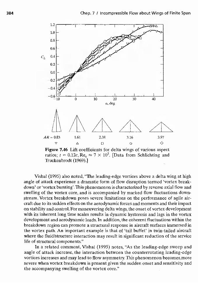
AR = 0.83 1.61 2.38 3.16 3.97
V 0 0
Figure 7.46 Lift coefficients for delta wings of various aspectratios; t = O.12c, 7 x [Data from Schlichting andTruckenbrodt (1969).]
Visbal (1995) also noted, "The leading-edge vortices above a delta wing at highangle of attack experience a dramatic form of flow disruption termed 'vortex break-down' or 'vortex bursting'.This phenomenon is characterized by reverse axial flow andswelling of the vortex core, and is accompanied by marked flow fluctuations down-stream. Vortex breakdown poses severe limitations on the performance of agile air-craft due to its sudden effects on the aerodynamic forces and moments and their impacton stability and control. For maneuvering delta wings, the onset of vortex developmentwith its inherent long time scales results in dynamic hysteresis and lags in the vortexdevelopment and aerodynamic loads. In addition, the coherent fluctuations within thebreakdown region can promote a structural response in aircraft surfaces immersed inthe vortex path. An important example is that of 'tail buffet' in twin-tailed aircraftwhere the fluid/structure interaction may result in significant reduction of the servicelife of structural components."
In a related comment, Visbal (1995) notes, "As the leading-edge sweep andangle of attack increase, the interaction between the counterrotating leading-edgevortices increases and may lead to flow asymmetry. This phenomenon becomesmoresevere when vortex breakdown is present given the sudden onset and sensitivity andthe accompanying swelling of the vortex core."
384 Chap. 7 / Incompressible Flow about Wings of Finite Span
1.2
1.0
0.8
0.6
CL 0.4
0.2
0.0
—0.2
—0.4
—0.6—10 20
a, deg
A
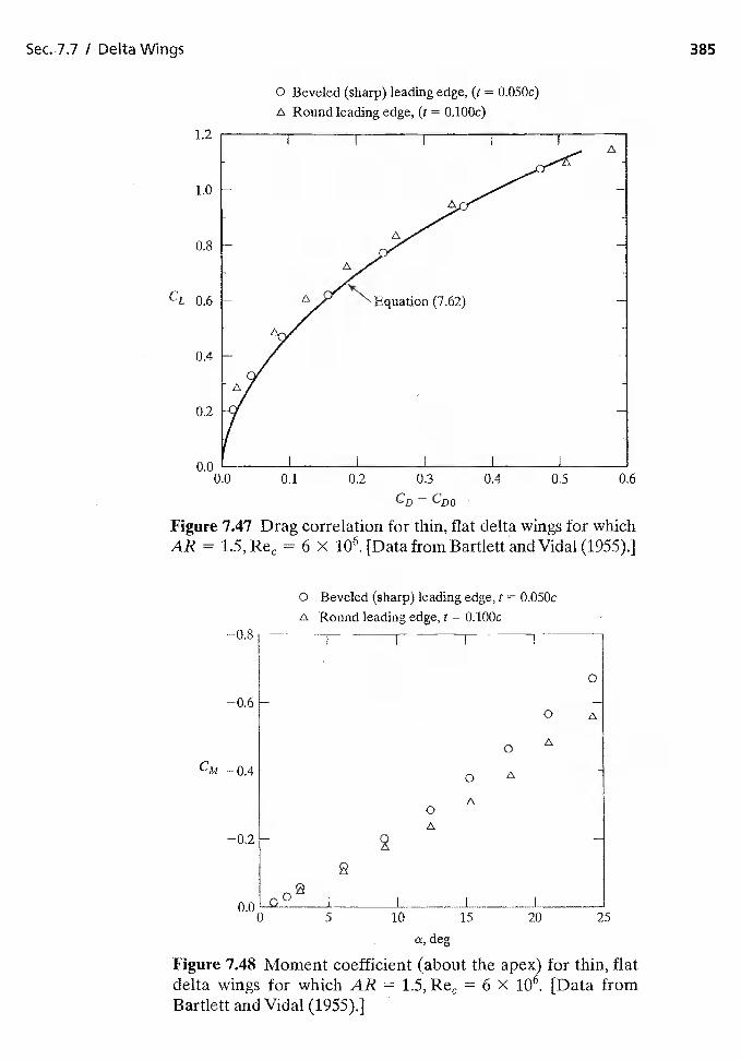
Sec.7.7 / Delta Wings 385
0 Beveled (sharp) leading edge, (t = 0.050c)
A Round leading edge, (t = 0.lOOc)
Figure 7.47 Drag correlation for thin, flat delta wings for whichAR = 1.5, = 6 x 10⁶. [Data from Bartlett and Vidal (1955).]
O Beveled (sharp) leading edge, t = O.050c
Round leading edge, t = 0.lOOc
a, deg
Figure 7.48 Moment coefficient (about the for thin, flatdelta wings for which AR 1.5, 6 X 10, [Data fromBartlett and Vidal (1955).]
1.2
1.0
0.8
CL 0.6
0.2
0.00.0 0.1 0.2 0.3 0.4 0.5
CD-CDO0.6
—0.8
0
—0.6 - —
0 A
A
CM04 0 A
0A
—0.2 -
I
5 10 15 20 25
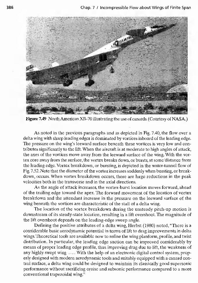
386 Chap. 7 / Incompressible Flow about Wings of Finite Span
As noted in the previous paragraphs and as depicted in Fig. 7.40, the flow over adelta wing with sharp leading edges is dominated by vortices inboard of the leading edge.The pressure on the wing's leeward surface beneath these vortices is very low and con-tributes significantly to the lift. When the aircraft is at moderate to high angles of attack,the axes of the vortices move away from the leeward surface of the wing. With the vor-tex core away from the surface, the vortex breaks down, or bursts, at some distance fromthe leading edge. Vortex breakdown, or bursting, is depicted in the water-tunnel flow ofFig. 7.52. Note that the diameter of the vortex increases suddenly when bursting, or break-down, occurs. When vortex breakdown occurs, there are large reductions in the peakvelocities both in the transverse and in the axial directions.
As the angle of attack increases, the vortex-burst location moves forward, aheadof the trailing edge toward the apex. The forward movement of the location of vortexbreakdown and the attendant increase in the pressure on the leeward surface of thewing beneath the vortices are characteristic of the stall of a delta wing.
The location of the vortex breakdown during the unsteady pitch-up motion isdownstream of its steady-state location, resulting in a lift overshoot. The magnitude ofthe lift overshoot depends on the leading-edge sweep angle.
Defining the positive attributes of a delta wing, Herbst (1980) noted, "There is aconsiderable basic aerodynamic potential in terms of lift to drag improvements in deltawings. Theoretical tools are available now to refine the wing planform, profile, and twistdistribution. In particular, the leading edge suction can be improved considerably bymeans of proper leading edge profile, thus improving drag due to lift, the weakness ofany highly swept wing ... . With the help of an electronic digital control system, prop-erly designed with modern aerodynamic tools and suitably equipped with a canard con-trol surface, a delta wing could be designed to maintain its classically good supersonicperformance without sacrificing cruise and subsonic performance compared to a moreconventional trapezoidal wing."
Figure 7.49 North American XB-70 illustrating the use of canards. (Courtesy of NASA.)
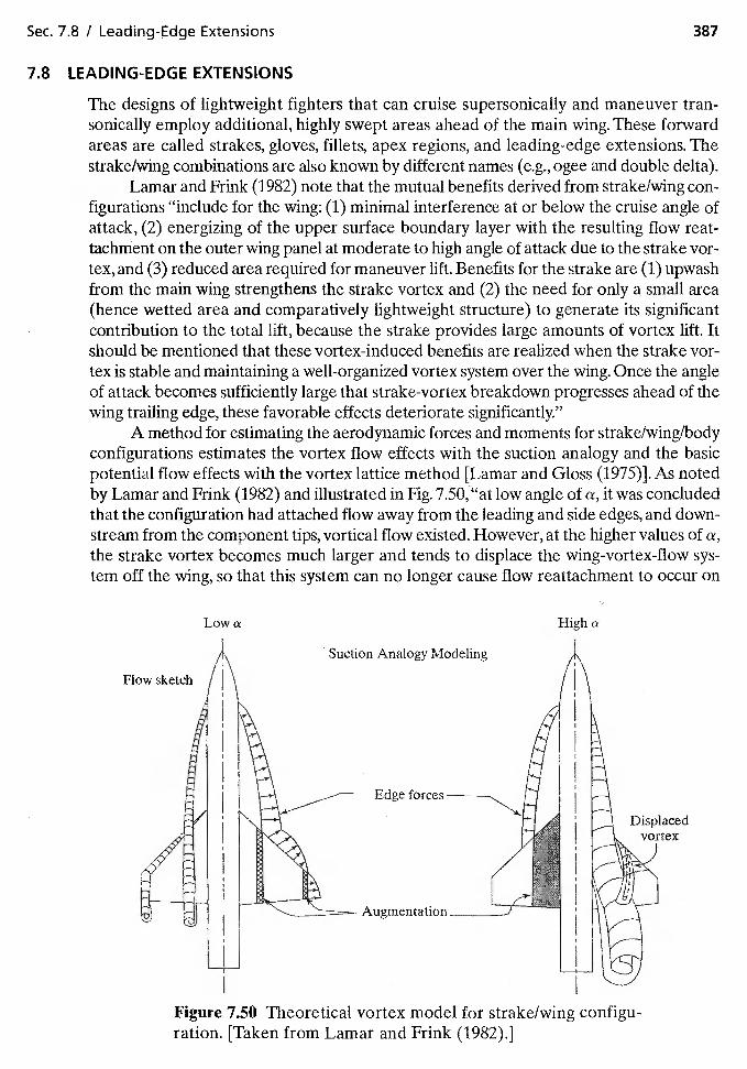
Sec. 7.8 I Leading-Edge Extensions 387
7.8 LEADING-EDGE EXTENSIONS
The designs of lightweight fighters that can cruise supersonically and maneuver tran-sonically employ additional, highly swept areas ahead of the main wing. These forwardareas are called strakes, gloves, fillets, apex regions, and leading-edge extensions. Thestrake/wing combinations are also known by different names (e.g., ogee and double delta).
Lamar and Frink (1982) note that the mutual benefits derived from strake/wing con-figurations "include for the wing: (1) minimal interference at or below the cruise angle ofattack, (2) energizing of the upper surface boundary layer with the resulting flow reat-tachment on the outer wing panel at moderate to high angle of attack due to the strake vor-tex, and (3) reduced area required for maneuver lift. Benefits for the strake are (1) upwashfrom the main wing strengthens the strake vortex and (2) the need for only a small area(hence wetted area and comparatively lightweight structure) to generate its significantcontribution to the total lift, because the strake provides large amounts of vortex lift. Itshould be mentioned that these vortex-induced benefits are realized when the strake vor-tex is stable and maintaining a well-organized vortex system over the wing. Once the angleof attack becomes sufficiently large that strake-vortex breakdown progresses ahead of thewing trailing edge, these favorable effects deteriorate significantly."
A method for estimating the aerodynamic forces and moments for strake/wingf bodyconfigurations estimates the vortex flow effects with the suction analogy and the basicpotential flow effects with the vortex lattice method [Lamar and Gloss (1975)]. As notedby Lamar and Frink (1982) and illustrated in Fig. 7.50,"at low angle of a, it was concludedthat the configuration had attached flow away from the leading and side edges, and down-stream from the component tips, vortical flow existed. However, at the higher values of a,the strake vortex becomes much larger and tends to displace the wing-vortex-flow sys-tem off the wing, so that this system can no longer cause flow reattachment to occur on
Displacedvortex
Figure 7.50 Theoretical vortex model for strake/wing configu-ration. [Taken from Lamar and Frink (1982).]
Flow sketch
Low a High a
Suction Analogy Modeling
Edge
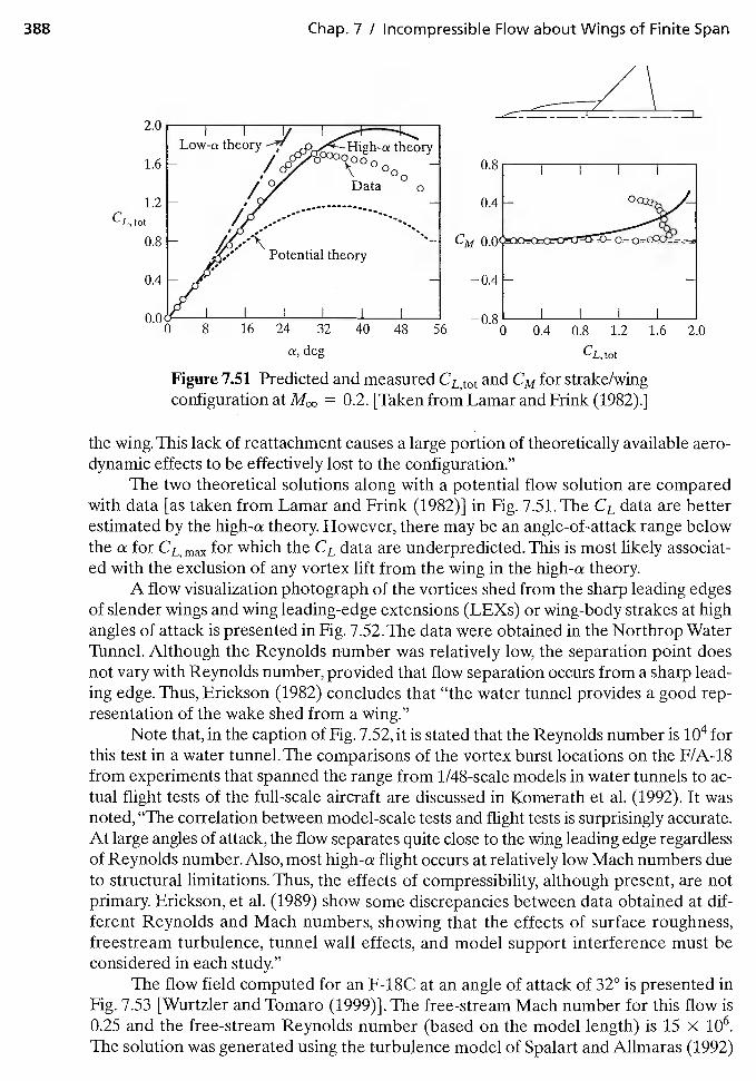
388 Chap. 7 I Incompressible Flow about Wings of Finite Span
1.2CL,tot
0.8 CM 0.0
—0.80 0.4 0.8 1.2 1.6 2.0
Figure 7.51 Predicted and measured CL,tot and CM for strake/wingconfiguration at = 0.2. [Taken from Lamar and Frink (1982).]
the wing. This lack of reattachment causes a large portion of theoretically available aero-dynamic effects to be effectively lost to the configuration."
The two theoretical solutions along with a potential flow solution are comparedwith data [as taken from Lamar and Frink (1982)1 in Fig. 7.51. The CL data are betterestimated by the high-a theory. However, there may be an angle-of-attack range belowthe a for CL data are underpredicted. This is most likely associat-ed with the exclusion of any vortex lift from the wing in the high-a theory.
A flow visualization photograph of the vortices shed from the sharp leading edgesof slender wings and wing leading-edge extensions (LEX5) or wing-body strakes at highangles of attack is presented in Fig. 7.52. The data were obtained in the Northrop WaterTunnel. Although the Reynolds number was relatively low, the separation point doesnot vary with Reynolds number, provided that flow separation occurs from a sharp lead-ing edge. Thus, Erickson (1982) concludes that "the water tunnel provides a good rep-resentation of the wake shed from a wing."
Note that, in the caption of Fig. 7.52, it is stated that the Reynolds number is forthis test in a water tunnel. The comparisons of the vortex burst locations on the F/A-18from experiments that spanned the range from 1/48-scale models in water tunnels to ac-tual flight tests of the full-scale aircraft are discussed in Komerath et al. (1992). It wasnoted, "The correlation between model-scale tests and flight tests is surprisingly accurate.At large angles of attack, the flow separates quite close to the wing leading edge regardlessof Reynolds number. Also, most high-a flight occurs at relatively low Mach numbers dueto structural limitations. Thus, the effects of compressibility, although present, are notprimary. Erickson, et al. (1989) show some discrepancies between data obtained at dif-ferent Reynolds and Mach numbers, showing that the effects of surface roughness,freestream turbulence, tunnel wall effects, and model support interference must beconsidered in each study."
The flow field computed for an F-18C at an angle of attack of 32° is presented inFig. 7.53 [Wurtzler and Tomaro (1999)]. The free-stream Mach number for this flow is0.25 and the free-stream Reynolds number (based on the model length) is 15 X 106.The solution was generated using the turbulence model of Spalart and Ailmaras (1992)
0.8I I
0.4 -
—0.4 -
I I
deg CL, tOt
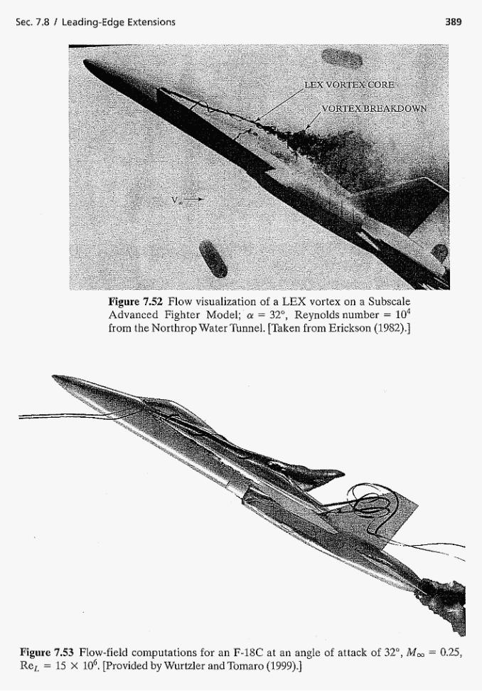
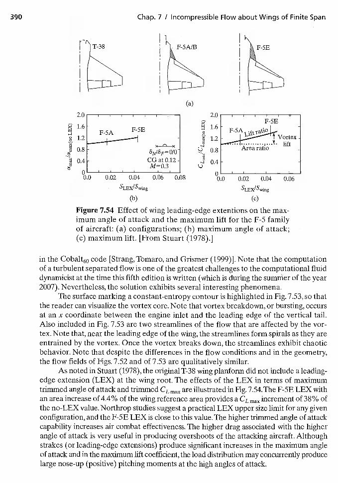
390 Chap. 7 / Incompressible Flow about Wings of Finite Span
2.0 2.0
1.6
j1.20.8 0.8
0.4-I I I
0 I
0.0 0.02 0.04 0.06 0.08 0.0 0.02 0.04 0.06
SLEx/Swing SLEx/Swing
(b) (c)
Figure 7.54 Effect of wing leading-edge extentions on the max-imum angle of attack and the maximum lift for the F-5 familyof aircraft: (a) configurations; (b) maximum angle of attack;(c) maximum lift. [From Stuart (1978).]
in the Cobalt60 code {Strang,Tomaro, and Grismer (1999)]. Note that the computationof a turbulent separated flow is one of the greatest challenges to the computational fluiddynamicist at the time this fifth edition is written (which is during the summer of the year2007). Nevertheless, the solution exhibits several interesting phenomena.
The surface marking a constant-entropy contour is highlighted in Fig. 7.53, so thatthe reader can visualize the vortex core. Note that vortex breakdown, or bursting, occursat an x coordinate between the engine inlet and the leading edge of the vertical tail.Also included in Fig. 7.53 are two streamlines of the flow that are affected by the vor-tex. Note that, near the leading edge of the wing, the streamlines form spirals as they areentrained by the vortex. Once the vortex breaks down, the streamlines exhibit chaoticbehavior. Note that despite the differences in the flow conditions and in the geometry,the flow fields of Figs. 7.52 and of 7.53 are qualitatively similar.
As noted in Stuart (1978), the original T-38 wing planform did not include a leading-edge extension (LEX) at the wing root. The effects of the LEX in terms of maximumtrimmed angle of attack and trimmed CL max are ifiustrated in Fig. 7.54.The F-5E LEX withan area increase of 4.4% of the wing reference area provides a CL max increment of 38% ofthe no-LEX value. Northrop studies suggest a practical LEX upper size limit for any givenconfiguration, and the F-SE LEX is close to this value, The higher trimmed angle of attackcapability increases air combat effectiveness. The higher drag associated with the higherangle of attack is very useful in producing overshoots of the attacking aircraft. Althoughstrakes (or leading-edge extensions) produce significant increases in the maximum angleof attack and in the maximum lift coefficient, the load distribution may concurrently producelarge nose-up (positive) pitching moments at the high angles of attack.
'T-38 F-SE
(a)
F-SEF-5AIIx x
CG at 0.12M=0.3
I I
F-SE
Area ratio
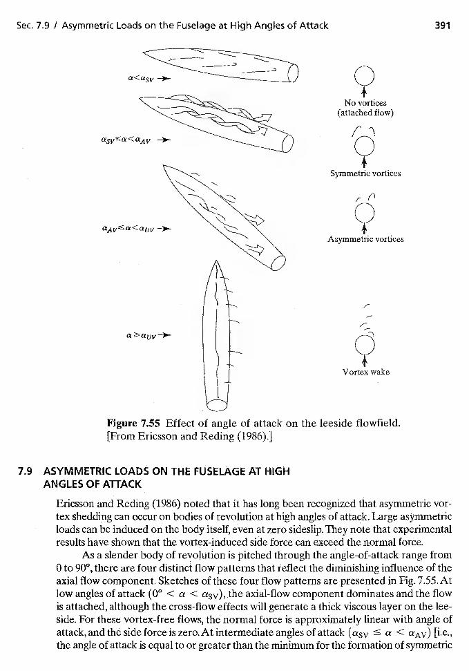
Sec. 7.9 / Asymmetric Loads on theFuselage at High Angles of Attack 391
7.9 ASYMMETRIC LOADS ON THE FUSELAGE AT HIGHANGLES OF ATFACK
Ericsson and Reding (1986) noted that it has long been recognized that asymmetric vor-tex shedding can occur on bodies of revolution at high angles of attack. Large asymmetricloads can be induced on the body itself, even at zero sideslip. They note that experimentalresults have shown that the vortex-induced side force can exceed the normal force.
As a slender body of revolution is pitched through the angle-of-attack range from0 to 90°, there are four distinct flow patterns that reflect the diminishing influence of theaxial flow component. Sketches of these four flow patterns are presented in Fig. 7.55.Atlow angles of attack (0° <a <aSv), the axial-flow component dominates and the flowis attached, although the cross-flow effects will generate a thick viscous layer on the lee-side. For these vortex-free flows, the normal force is approximately linear with angle ofattack, and the side force is zero. At intermediate angles of attack (asy � a <aAy) [i.e.,the angle of attack is equal to or greater than the minimum for the formation of symmetric
<aAV
No vortices(attached flow)
Symmetric vortices
Asymmetric vortices
Vortex wake
a
Figure 7.55 Effect of angle of[From Ericsson and Reding (1986).]
attack on the leeside flowfield.
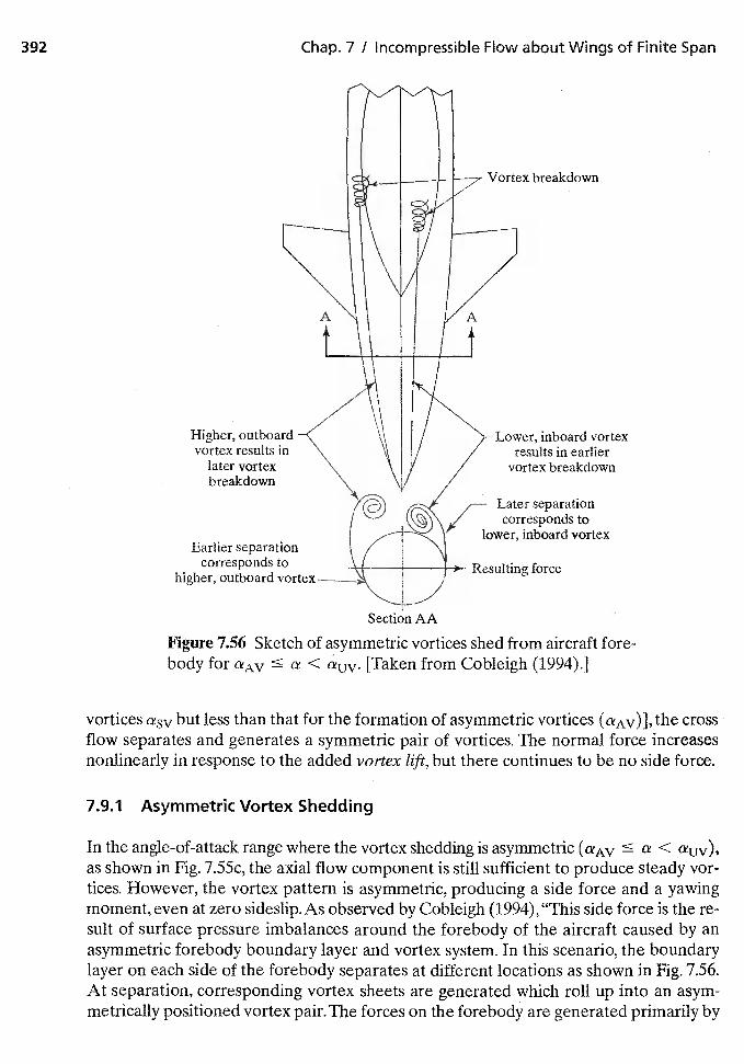
392 Chap. 7 / Incompressible Flow about Wings of Finite Span
Higher, outboardvortex results in
later vortexbreakdown
Earlier separationcorresponds to
higher, outboard vortex
Lower, inboard vortexresults in earlier
vortex breakdown
Later separationcorresponds to
lower, inboard vortex
Resulting force
Figure 7.56 Sketch of asymmetric vortices shed from aircraft fore-body for aAV a < aUV. [Taken from Cobleigh (1994).]
vortices aSV but less than that for the formation of asymmetric vortices (aAV)], the crossflow separates and generates a symmetric pair of vortices. The normal force increasesnonlinearly in response to the added vortex lift, but there continues to be no side force.
7.9.1 Asymmetric Vortex Shedding
In the angle-of-attack range where the vortex shedding is asymmetric (QAV a < auv),as shown in Fig. 7.55c, the axial flow component is still sufficient to produce steady vor-tices. However, the vortex pattern is asymmetric, producing a side force and a yawingmoment, even at zero sideslip.As observed by Cobleigh (1994), "This side force is the re-sult of surface pressure imbalances around the forebody of the aircraft caused by anasymmetric forebody boundary layer and vortex system. In this scenario, the boundarylayer on each side of the forebody separates at different locations as shown in Fig. 7.56.At separation, corresponding vortex sheets are generated which roll up into an asym-metrically positioned vortex pair.The forces on the forebody are generated primarily by
Vortex breakdown
Section AA

Sec. 7.9 I Asymmetric Loads on the Fuselage at High Angles of Attack 393
80
70 —0— Unmodified forebody
60 —a-— FB and NB transition grit
a 50—0—- Si strake; NB grit
40S2 strake; FB and NB grit
30
20—0.10 —0.05 0.00 0.05 0.10
Cf0
Figure 7.57 Variation of yawing moment asymmetry with angle ofattack for an X-31 for a 1-g maneuver. from Cobleigh (1994).]
the boundary layer and to a lesser extent by the vortices, depending on their proximityto the forebody surface. Fig 7.56 shows a typical asymmetrical arrangement where thelower, more inboard vortex corresponds to a boundary layer which separates later and,conversely, the higher, more outboard vortex corresponds to the boundary layer whichseparated earlier. The suction generated by the more persistent boundary layer and thecloser vortex combine to create a net force in their direction. Since the center of gravityof the aircraft is well aft of the forebody, a sizeable yawing moment asymmetry develops."
There are a variety of techniques that can be used to modify the asymmetric vor-tex pattern, including physical surfaces, such as strakes, and boundary-layer control, suchas blowing or suction at the surface. The yawing moment asymmetry for an X-31 dur-ing slow decelerations (essentially ig) to high AOA (angle of attack) conditions, as takenfrom Cobleigh (1994), is reproduced in Fig. 7.57. For the basic aircraft, the asymmetricforces started to build up, beginning at an angle of attack of 48° reaching a peak valueof (the yawing moment coefficient at zero sideslip) of —0.063 at an angle of attackof approximately 57°.The asymmetric forces decreased rapidly with alpha, becoming rel-atively small by an angle of attack of 66°. In an attempt to reduce these asymmetries, tran-sition grit strips were installed on both sides of the forebody (FB) and along the sidesof the nose boom (NB). The data indicated that the side forces actually increased whengrit strips were used. Although the largest asymmetry began to build at the same angleof attack as for the basic aircraft (an AOA of 48°), the peak asymmetry increased toof —0.078. For the aircraft with these transition strips, the largest asymmetry occurredin the alpha range from 58° to 61°. The use of a strake along with blunting of the nosetip delayed the initiation of the yawing moment asymmetry up to an AOA of 55° (referto Fig. 7.57). The peak asymmetric yawing moment coefficient of —0.040 occurredat an angle of attack of 60°, after which the asymmetric yawing moment coefficientdecreased. As evident in the data presented in Fig. 7.57, the use of both a strake andboundary-layer transition strips produced significant yawing moments which persistedover a broad angle-of-attack range.
In summary, Cobleigh (1994) reported, "Several aerodynamic modifications weremade to the X-31 forebody with the goal of minimizing the asymmetry. A method fordetermining the yawing moment asymmetry from flight data was developed and ananalysis of the various configuration changes completed. The baseline aircraft were
394 Chap. 7 I Incompressible Flow about Wings of Finite Span
found to have significant asymmetries above 45° -angle of attack with the largest asym-metry typically occurring around 600 -angle of attack. Applying symmetrical bound ary-layer transition strips along the forebody sides increased the magnitude of the asymmetryand widened the angle-of-attack range over which the largest asymmetry acted. Installinglongitudinal forebody strakes and rounding the sharp nose of the aircraft caused theyawing moment asymmetry magnitude to be reduced. The transition strips and strakesmade the asymmetry characteristic of the aircraft more repeatable than the clean fore-body configuration. Although no geometric differences between the aircraft were known,ship 2 consistently had larger yawing moment asymmetries than ship 1,"
For axisymmetric bodies with wings or fins, the interaction with the asymmetric vor-tex pattern can produce rolling moments. Typically, the effectiveness of the vertical tailand rudder to control the yawing moment falls off as the angle of attack increases,because the vertical tail lies in the wake of the wing and of the fuselage.
Ericsson and Reding (1986) note that "the seriousness of the problem is illustratedby the wind-tunnel test results for the F-ill, which show the vortex-induced yawing mo-ment to exceed, by an order of. magnitude, the available control capability through fullrudder deflection. The problem can be cured by use of nose strakes or other types of bodyreshaping that cause the forebody vortices to be shed symnietrically."
An article by Dornheim (1994) included the paragraph, "The X-3i's main prob-lem is directional instability from asymmetric nose vortices around 60 deg.AOA, whichcaused an unintended departure in flight test. At that 165 knots condition, the yawmoment from the vortices was estimated to be 2.5 times more powerful than the thrustvectoring, and as powerful as therudder itself would be at 10 deg. AOA. A subtlereshaping of the nose and adding vortex control strakes has tamed the vortices, and theX-31 should be able to fly at least 300 knots, where the 6g structural limit comes into play,before the remaining vortices can overpower the thrust vectoring at high AOA."
7.9.2 Wakelike Flows
Fmaily, at very high angles of attack � < 90°) the axial-flow component has lessand less influence, so that the vortex shedding becomes unsteady, starting on the aft bodyand progressing toward the nose with increasing angle of attack. In this angle-of-attackrange, the leeside flow resembles the wake of a two-dimensional cylinder normal to theflow. The mean side force decreasestoward zero inthis angle-of-attack range.
7.10 FLOW FIELDS FOR AIRCRAFT AT HIGH ANGLES OFA1TACK
As noted by Mendenhall and Perkins (1996), "Many modern high-performance fighteraircraft have mission requirements which necessitate rapid maneuvers at high angles ofattack and large angular rotation rates. Under these flow conditions, the vehicle mayoperate in a flow regime in which the aerodynamic characteristics are dominated byunsteady nonlinear effects induced by flow separation, vortex shedding, and vortex lageffects (Fig. 7.58). During extreme multiple-axis maneuvering conditions, the dynamicand time-dependent effects of these nonlinear flow characteristics contribute significantlyto the behavior and maneuvering capability of aircraft."
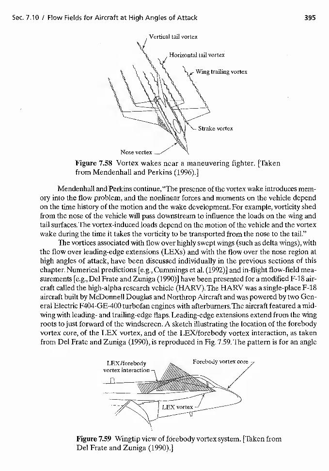
Sec. 7.10 I Flow Fields for Aircraft at High Angles of Attack 395
Vertical tail vortex
Horizontal tail vortex
Wing trailing vortex
Strake vortex
Figure 7.58 Vortex wakes near a maneuvering fighter. [Takenfrom Mendenhall and Perkins (1996).]
Mendenhall and Perkins continue, "The presence of the vortex wake introduces mem-ory into the flow problem, and the nonlinear forces and moments on the vehicle dependon the time history of the motion and the wake development. For example, vorticity shedfrom the nose of the vehicle will pass downstream to influence the loads on the wing andtail surf aces. The vortex-induced loads depend on the motion of the vehicle and the vortexwake during the time it takes the vorticity to be transported from the nose to the tail."
The vortices associated with flow over highly swept wings (such as delta wings), withthe flow over leading-edge extensions (LEXs) and with the flow over the nose region athigh angles of attack, have been discussed individually in the previous sections of thischapter. Numerical predictions [e.g., Cummings et al. (1992)] and in-flight flow-field mea-surements [e.g., Del Frate and Zuniga (1990)] have been presented for a modified F-18 air-craft called the high-alpha research vehicle (HARV).The HARV was a single-place F-18aircraft built by McDonnell Douglas and Northrop Aircraft and was powered by two Gen-eral Electric F404-GE-400 turbofan engines with afterburners. The aircraft featured a mid-wing with leading- and trailing-edge flaps. Leading-edge extensions extend from the wingroots to just forward of the windscreen.A sketch illustrating the location of the forebodyvortex core, of the LEX vortex, and of the LEX/forebody vortex interaction, as takenfrom Del Frate and Zuniga (1990), is reproduced in Fig. 7.59. The pattern is for an angle
Figure 759 Wingtip view of fOrebody vortex system. [Taken fromDel Frate and Zuniga (1990).]
Nose vortex
LEX/forebodyvortex interaction
Forebody vortex core
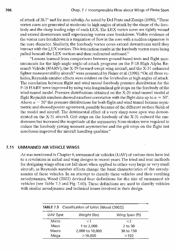
396 Chap. 7 / Incompressible Flow about Wings of Finite Span
of attack of 38.7° and for zero sideslip. As noted by Del Frate and Zuniga (1990), "Thesevortex cores are generated at moderate to high angles of attack by the shape of the fore-body and the sharp leading edge of each LEX. The LEX vortex cores are tightly woundand extend downstream until experiencing vortex core breakdown. Visible evidence ofthe vortex core breakdown is a stagnation of flow in the core with a sudden expansion inthe core diameter. Similarly, the forebody vortex cores extend downstream until theyinteract with the LEX vortices, This interaction results in the forebody vortex cores beingpulled beneath the LEX vortices and then redirected outboard."
"Lessons learned from comparisons between ground-based tests and flight mea-surements for the high-angle-angle-of-attack programs on the F-18 High Alpha Re-search Vehicle (HARV), the X-29 forward-swept wing aircraft, and the X-31 enhancedfighter maneuverability aircraft" were presented by Fisher et al. (1998). "On all three ve-hicles, Reynolds number effects were evident on the forebodies at high angles of attack.The correlation between flight and wind tunnel forebody pressure distribution for theF-18 HARV were improved by using twin longitudinal grit strips on the forebody of thewind-tunnel model. Pressure distributions obtained on the X-29 wind-tunnel model atflight Reynolds numbers showed excellent correlation with the flight data up to a = 50°.Above a = 50° the pressure distributions for both flight and wind tunnel became asym-metric and showed poorer agreement, possibly because of the different surface finish ofthe model and aircraft. The detrimental effect of a very sharp nose apex was demon-strated on the X-31 aircraft. Grit strips on the forebody of the X-31 reduced the ran-domness but increased the magnitude of the asymmetry. Nose strakes were required toreduce the forebody yawing moment asymmetries and the grit strips on the flight testnoseboom improved the aircraft handling qualities."
7.11 UNMANNED AIR VEHICLE WINGS
As was mentioned in Chapter 6, unmanned air vehicles (UAV) of various sizes have ledto a revolution in airfoil and wing designs in recent years. The tried and true methodsfor designing wings often can fall short when applied to either very large or very smallaircraft, as Reynolds number effects change the basic characteristics of the aerody-namics of these vehicles. In an attempt to classify these vehicles and their resultingaerodynamics, Wood (2002) devised four definitions for the size of unmanned airvehicles (see Table 7.3 and Fig. 7.60). These definitions are used to classify vehicleswith similar aerodynamic and technical issues involved in their design.
TABLE 7.3 Classification of UAVs [Wood (2002)]
UAVType Weight (lbs) Wing Span (ft)
Micro <1 <2Meso 1 to 2,000 2 to 30Macro 2,000 to 10,000 3Oto 150Mega >10,000 >150
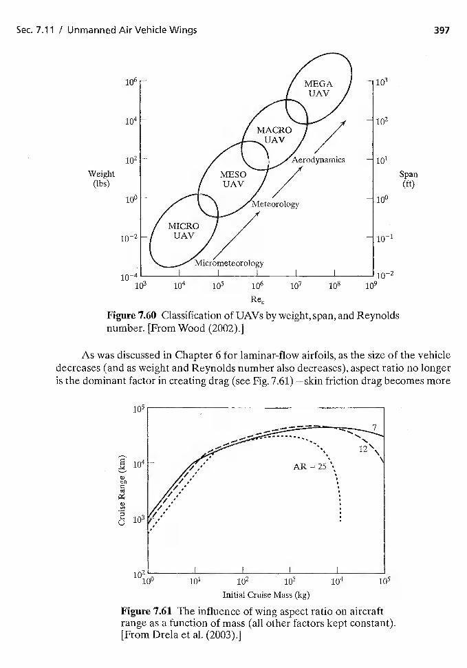
I I
106 108
Figure 7.60 Classification of UAVs by weight, span, and Reynoldsnumber. [From Wood (2002).]
As was discussed in Chapter 6 for laminar-flow airfoils, as the size of the vehicledecreases (and as weight and Reynolds number also decreases), aspect ratio no longeris the dominant factor in creating drag (see Fig. 7.61)—skin friction drag becomes more
Figure 7.61 The influence of wing aspect ratio on aircraftrange as a function of mass (all other factors kept constant).[From Drela et al, (2003).]
Sec. 7.11 / Unmanned Air Vehicle Wings 397
106 -
- 102
102 - —
Weight Span(ibs) (ft)
10° 10°
102102 1o4
Initial Cruise Mass (kg)
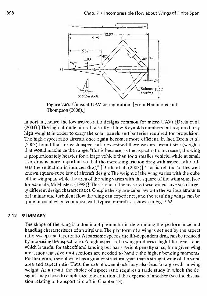
398 Chap. 7 / Incompressible Flow about Wings of Finite Span
Q
Figure 762 Unusual UAV configuration. [From Hammons andThompson (2006).]
important, hence the low aspect-ratio designs common for micro UAVs [Drela et al.(2003).] The high-altitude aircraft also fly at low Reynolds numbers but require fairlyhigh weights in order to carry the solar panels and batteries required for propulsion.The high-aspect ratio aircraft once again becomes mOre efficient. In fact, Drela et al.(2003) found that for each aspect ratio examined there was an aircraft size (weight)that would maximize the range: "this is because, as the aspect ratio increases, the wingis proportionately heavier for a large vehicle than for a smaller vehicle, while at smallsize, drag is more important so that the increasing friction drag with aspect ratio off-sets the reduction in induced drag" [Drela et at. (2003)]. This is related to the wellknown square-cube law of aircraft design: The weight of the wing varies with the cubeof the wing span while the area of the wing varies with the square of the wing span [seefor example, McMasters (1998)].This is one of the reasons these wings have such large-ly different design characteristics. Couple the square-cube law with the various amountsof laminar and turbulent flow the wing can experience, and the resulting wings can bequite unusual when compared with typical aircraft, as shown in Fig. 7.62.
7.12 SUMMARY
The shape of the wing is a dominant parameter in determining the performance andhandling characteristics of an airplane. The planform of a wing is defined by the aspectratio, sweep, and taper ratio. At subsonic speeds, the lift-dependent drag can be reducedby increasing the aspect ratio. A high-aspect-ratio wing produces a high-lift-curve slope,which is useful for takeoff and landing but has a weight penalty since, for a given wingarea, more massive root sections are needed to handle the higher bending moments.Furthermore, a swept wing has a greater structural span than a straight wing of the samearea and aspect ratio. Thus, the use of sweepback may also lead to a growth in wingweight. As a result, the choice of aspect ratio requires a trade study in which the de-signer may chose to emphasize one criterion at the expense of another (see the discus-sion relating to transport aircraft in Chapter 13).
-I
Problems 399
Tapering the wing reduces the wing-root bending moments, since the inboard por-tion of the wing carries mOre of the wing's lift than the portion near the tip. While taperreduces the actual loads carried by the outboard sections, the wing-tip sections are sub-jected to higher lift coefficients and tend to stall first (see Fig. 7.18). Thus, progressivelyreducing the incidence of the local section through the use of geometric twist from the rootto the tip (i.e.,washout) may be used either to reduce local loading or to prevent tip stalling.
PROBLEMS
7.1. Consider an airplane that weighs 14,700 N and cruises in level flight at 300 km/h at an alti-tude of 3000 m. The wing has a surface area of 17.0 m2 and an aspect ratio of 6.2. Assumethat the lift coefficient is a linear function of the angle of attack and that = —1.2°. If theload distribution is elliptic, calculate the value of the circulation in the plane of symmetry(F0), the downwash velocity the induced-drag coefficient (CDV), the geometric angleof attack (cr), and the effective angle of attack (ae).
7.2. Consider the case where the spanwise circulation distribution for a wing is parabolic,
If the total lift generated by the wing with the parabolic circulation distribution is to beequal to the total lift generated by a wing with an elliptic circulation distributIon, what is therelation between the F0 values for the two distributions? What is the relation between theinduced downwash velocities at the plane of symmetry for the two configurations?
7.3. When a GA(W)-1 airfoil section (i.e., a wing of infinite span) is at an angle of attack of 4°,the lift coefficient is 1.0. Using equation (7.20), calculate the angle of attack at which a wingwhose aspect ratio is 7.5 would have to operate to generate the same lift coefficient. Whatwould the angle of attack have to be to generate this lift coefficient for a wing whose aspectratio is 6.0?
7.4. Consider a planar wing (i.e.,no geometric twist) which has a NACA 0012 section and an aspectratio of 7.0. Following Example 7.1, use a four-term series to represent the load distribution.Compare the lift coefficient; the induced-drag coefficient, and the spanwise lift distribution fortaper ratios of (a) 0.4, (b) 0.5, (c) 0.6, and (d) 1.0.
7.5. Consider an airplane that weighs 10,000 N and cruises in level flight at 185 km/h at analtitude of 3.0 km.The wing has a surface area of 16.3 m2, an aspect ratio of 7.52, and a taperratio of 0.69. Assume that the lift coefficient is a linear function of the angle of attack andthe airfoil section is a NACA 2412 (see Chapter 6 for the characteristics of this section).The incidence of the root section is + 1.5°; the incidence of the tip section is —1.5°. Thus,there is a geometric twist of —3° (washout). Following Example 7.1, use a four-term seriesto represent the load distribution and calculate(a) The lift coefficient (CL)(b) The spanwise load distribution (Cl(y)/CL)(c) The induced drag coefficient (CDV)(d) The geometric angle of attack (a)
7.6. Use equation (7.37) to calculate the velocity induced at some point C(x, y, z) by the vortexfilament AB (shown in Fig. 7.29); that is, derive equation (7.38a).
7.7. Use equation (7.37) to calculate the velocity induced at some point C(x, y, 0) by the vortexfilament AB in a planar wing; that is, derive equation (7.43a).
400 Chap. 7 / Incompressible Flow about Wings of Finite Span
7.8. Calculate the downwash velocity at the CP of panel 4 induced by the horseshoe vortex ofpanel 1 of the starboard wing for the flow configuration of Example 7.2.
7.9. Following the VLM approach used in Example 7.2, calculate the lift coefficient for a sweptwing. The wing has an aspect ratio of 8, a taper ratio of unity (i.e., = ce), and an uncamberedsection (i.e., it is a flat plate). Since the taper ratio is unity, the leading edge, the quarter-chordline, the three-quarter chord line, and the trailing edge all have the same sweep, 45°. HOw doesthe lift coefficient for this aspect ratio (8) compare with that for an aspect ratio of 5 (i.e., thatcomputed iii Example 7.2)? Is this consistent with our knowledge of the effect of aspect ratio(e.g., Fig. 7.10)?
7.10. Following the \'LM approach used in Example 7.2, calculate the lift coefficient for a sweptwing. The wing has an aspect ratio of 5, a taper ratio of 0.5 (i.e., = 0.5 ci), an uncamberedsection, and the quarter chord is swept 45°. Since the taper ratio is not unity, the leading edge,the quarter-chord line, the three-quarter-chord line, and the trailing edge have differentsweep angles.This should be taken into account when defining the coordinates of the horse-shoe vortices and the control points.
7.11. Following the VLM approach used in Example 7.2, calculate the lift coefficient for the forwardswept wing of Fig. 7.23b. The quarter chord is swept forward 45°, the aspect ratio is 3.55. andthe taper ratio 0.5. The airfoil section (perpendicular to the quarter chord) is a NACA 64A1 12.For this airfoil section a02 —0.94° and = 6.09 per radian. For purposes of applying theno-flow boundary condition at the control points, assume that the wing is planar. Prepare agraph of the lift coefficient. How does this compare with that of Fig. 7.23?
7.12. Following the VLM approach used in Example 7.2, calculate the lift coefficient for a deltawing whose aspect ratio is 1.5. What is the sweep angle of the leading edge? The fact thatthe quarter-chord and the three-quarter-chord lines have different sweeps should be takeninto account when defining the coordinates of the horseshoe vortices and the control points.How do the calculated values for the lift coefficient compare with the experimental valuespresented in Fig. 7.44?
7.13. Use equation (7.61) to calculate the lift coefficient as a function of the angle of attack for aflat delta wing with sharp leading edges. The delta wing has an aspect ratio of 1.5. Comparethe solution with the data of Fig. 7.44.
7.14. Use equation (7.62) to calculate the induced drag for a flat delta wing with sharp leadingedges.The delta wing has an aspect ratio of 1.5. Compare the solution with the data of Fig. 7.47.
7.15. Assume that the wing area of an airplane is proportional to the square of the wing spanand the volume, and thus the weight, is proportional to the cube of the wing span (this isthe square-cube law). Find the wing loading of the aircraft as a function of wing span, b.Using these relationships explain why very large aircraft (like the Boeing 747 or the Air-bus 380) have to fly with very large wing loadings. If you wanted to re-design an existingaircraft that weighed 92,000 lbs with a wing span of 75 It, what wing span would you needto add an additional 10% to the weight?
REFERENCES
Abbott IH, von Doenhoff AB. 1949. Theory of Wing Sections. NewYork: Dover
Anderson SD, Corda S,Van Wie DM. 1980. Numerical lifting line theory applied to droopedleading-edge wings below and above stall. J. Aircraft 17:898—904
Bartlett GE,Vidal Ri 1955. Experimental investigations of influence of edge shape on the aero-dynamic characteristics of low aspect ratio wings at low speeds. J. Aeron. Set. 22:517—533,588
References 401
Bristow DR. Grose GG. 1978. Modification of the Douglas Neumann program to improvethe efficient of predicting component and high lift charactersitics. NASA CR 3020
Cubleigh BR 1994. High-angle-of-attack yawing moment asymmetry of the X-31 aircraftfrom flight test. Presented at Appi. Aerodyn. Conf., AIAA Pap. 94-1803, ColoradoSprings, CO
Cummings RM, Rizk YM, Schiff LB, Chaderjian NM. 1992. Navier-Stokes prediction for theF-18 wing and fuselage at large incidence. J. Aircraft 29:565—574
Del Frate JH, Zuniga FA. 1990. In-flight flow field analysis on the NASA F-18 high alpharesearch vehicle with comparison to the ground facility data. Presented at AIAA Aerosp.Sci. Meet., 28th, AIAA Pap. 90—0231, Reno, NV
Dornheim MA. 1994. X-31, F-16 MATV, FIA-18 HARV explore diverse missions. Aviat.Week Space Tech. 140:46—47
Drela M, Protz JM, Epstein AH. 2003.The role of size in the future of aeronautics. Presentedat Intl. Air Space Symp., AIAA Pap. 2003—2902, Dayton, OH
Ericsson LE, Reding JP. 1986. Asymmetric vortex shedding from bodies of revolution. InTactical Missile Aerodynamics, Ed. Hemsch MH, Nielsen JN. Washington, DC: AIAA
Erickson GE. 1982. Vortex flow correlation. Presented at Congr. Intl. Coun. Aeron. Sci.,ICAS Pap. 82—6.61, Seattle, WA
Erickson GE, Hall RM, Banks DW, DeiFrate JH, Schreiner JA, Hanley RJ, Pulley CT. 1989.Experimental investigation of the F/A-.18 vortex flows at subsonic through transonic speeds.Presented at Appi. Aerodyn. ConL, 7th, AIAA Pap. 89—2222, Seattle, WA
Falkner VM. 1943. The calculation of aerodynamic loading on surfaces of any shape. ARCR&M 1910
Fisher DF, Cobleigh BR, Banks, DW, Hall RM, Wahls RA. 1998. Reynolds number effectsat high angles of attack. Presented at Adv. Meas. Ground Test. Tech. Conf., 20th, AIAA Pap.98—2879, Albuquerque, NM
Gloss BB, Washburn KB. 1978. Load distribution on a close-coupled wing canard at tran-sonic speeds. J. Aircraft 15:234—239
Hammons C, Thompson DS. 2006. A numerical investigation of novel planforms for microPresented at AIAA Aerosp. Sci. Meet., AIAA Pap. 2006—1265, Reno, NV
Henderson WP. 1966. Studies of various factors affecting drag due to lift at subsonic speeds.NASA Tech. Note D-3584
Herbst WB. 1980. Future fighter tcchnologies. I. Aircraft 17:561—566
Hummel D. 2004. Effects of boundary layer formation on the vortical flow above a deltawing. Presented at NATO RTO Appl. Veh. Tech. Spec. Meet., RTO-MP-AVT-111, Paper30-1, Prague, Czech Republic.
Johnson FT. 1980. A general panel method for the analysis and design of arbitrary config-urations in incompressible flows. NASA CR 3079
Kalman TP, Giesing JP, Rodden WE 1970. Spanwise distribution of induced drag in subsonicflow by the vortex lattice method. J. Aircraft 7:574—576
Kalman TP, Rodden WE Giesing JP. 1971. Application of the doublet-lattice method tononpianar configurations in subsonic flow. J. Aircraft 8:406—413
Komerath NMS, Liou SG, Schwartz RJ, Kim JM. 1992. Flow over a twin-tailed aircraft atangle of attack; part I: spatial characteristic. J. Aircraft 29:413—420
402 Chap. 7 / Incompressible Flow about Wings of Finite Span
Lamar JE, Gloss BB. 1975. Subsonic aerodynamic characteristics of interacting lifting sur-faces with separated flow around sharp edges predicted by vortex-lattice method. NASATech. Note D-7921
Lamar JF, Frink NT 1982. Aerodynamic features of designed strake-wing configurations.J.Aircraft 19:639—646
Margason RJ, Lamar JE. 1971. Vortex-lattice Fortran program for estimating subsonicaerodynamic charactersitics of complex planforms. NASA Note D-6142
Margason RJ, Kjelgaard SO, Sellers WL, Morris CEK, Walkey KB, Shields EW. 1985. Sub-sonic panel methods—a comparison of several production codes. Presented at AIAAAerosp. Sci. Meet., AIAA Pap. 85—0280, Reno, NV
McKinney LW, Dollyhigh SM. 1971. Some trim drag considerations for maneuvering air-craft. J. Aircraft 8:623—629
McMasters JH.1998. Advanced configurations for very large transport airplanes. AircraftDesign 1:217—242
Mendenhall MR, Perkins SC. 1996. Predicted high-a aerodynamic characteristics ofmaneuvering aircraft. Presented at App!. Aerodyn;Conf., 14th, AIAA Pap. 96—2433,New Orleans, LAMulthopp H. 1950. Method for calculating the lift distribution of wings (subsonic liftingsurface theory). ARC T&M 2884
Orloff KL. 1980. Spanwise lift distribution on a wing from flowfield velocity surveys.J. Aircraft 17:875—882
Peckham DH. 1958. Low-speed wind tunnel tests on a series of uncambered slender point-ed wings with sharp edges. ARC R&M 3186
Phillips WF, Snyder DO. 2000. Application of lifting-line theory to systems of lifting sur-faces. Presented at AJAA Aerosp. Sci. Meet,, 38th AIAA Pap. 2000—0653, Reno, NV
Polhamus ED. 1971a. Predictions of vortex-lift characteristics by a leading-edge suctionanalogy. J. Aircraft 8:193-399
Poihamus ED. 1971b. Charts for predicting the subsonic vortex-lift characteristics of arrow,delta, and diamond wings. NASA Tech. Note D-6243
Prandtl L. 1921. Application of modern hydrodynamics to aeronautic& NACA Report 116
Prandtl L,Tietjens 0G. 1957.Applied Hydro- andAeromechanics. New York: Dover
Rasmussen ML, Smith DE. 1999. Lifting-line theory for arbitrarily shaped wings. J. Aircraft36:340—348
Robinson A, Laurmann JA. 1956. Wing Theory. Cambridge: Cambridge University Press
Schlichting H. 1960. Some developments in boundary layer research in the past thirty years.J. Roy. Aeron. Soc. 64:64-79
Schlichting H,Truckenbrodt E. 1969. A erodynamik des Flugzeuges. Berlin: Spring-Verlag
Sivells JC. 1947. Experimental and calculated characteristics of three wings of NACA64-210 and 65-210 airfoil sections with and without washout. NACA Tech. Note 1422
Spalart PR, Ailmaras R. 1992. A one-equation turbulence model for aerodynamics flows.Presented at AIAA Aerosp. Sci. Meet., 30th AIAA Pap. Reno, NV
Spreiter JR. Sacks, AH. 1951. The rolling up of the vortex sheet and its effect on thedownwash behinds wings. J.Aeron. Sci. 18:21—32
References 403
Stanbrook A, Squire LC. 1964. Possible types of flow at swept leading edges. The Aeron.Quart. 15:72-82
Strang WZ,Tomaro RF, Grismer MJ. 1999. The defining methods of Cobalt60: a parallel,implicit, unstructured EulerlNavier-Stokes flow solver. Presented at AIAA Aerosp. Sci.Meet., 37th,AIAA Pap. 99—0786, Reno, NV
Stuart WG. 1978. Northrop F-S Case Study in Aircraft Design. Washington, DC: AIAA
Visbal MR. 1995. Computational and physical aspects of vortex breakdown on delta wings.Presented at AIAA Aerosp. Sci. Meet., 33rd AIAA Pap. 95—0585, Reno, NV
Voight W. 1976. Gestation of the swallow. Air Intern. 10:135—139,153
Weber J, Brebner GG. 1958. Low-speed tests on 45-deg swept-back wings, part I: pressuremeasurements on wings of aspect ratio 5. ARC R&M 2882Wood RM. 2002. A discussion of aerodynamic control effectors for unmanned air vehicles.Presented at Tech. Conf. Workshop Unmanned Aerosp. Veh., AIAA Pap. 2002—3494,Portsmouth, VA
Wurtzler KE, Tomaro RE 1999. Unsteady aerodynamics of aircraft maneuvering at highangle of attack. Presented at DoD High Perf. Comp. User's Group Meet., Monterey, CA
8 DYNAMICS OF A
COMPRESSIBLE FLOW FIELD
Thus far, we have studied the aerodynamic forces for incompressible (constant density)flows past the vehicle. At low flight Mach numbers (e.g., below a free-stream Mach num-ber of approximately 0.3 to 0.5), Bernoulli's equation [equation (3.10)] providesthe relation between the pressure distribution about an aircraft and the local velocitychanges of the air as it flows around the various components of the vehicle. However,as the flight Mach number increases, changes in the local air density also affect the mag-nitude of the local static pressure. This leads to discrepancies between the actual aero-dynamic forces and those predicted by incompressible flow theory. For our purposes, theMach number is the parameter that determines the extent to which compressibilityeffects are important. The purpose of this chapter is to introduce those aspects of com-pressible flows (i.e., flows in which the density is not constant) that have applications toaerodynamics
Throughout this chapter, air will be assumed to behave as a thermally perfect gas(i.e., the gas obeys the equation of state):
p = pRT (1.10)
We will assume that the gas is also calorically perfect; that is, the specific heats, andof the gas are constant. These specific heats are discussed further in the next sec-
tion. The term perfect gas will be used to describe a gas that is both thermally andcalorically perfect.
404
Sec. 8.1 I Thermodynamic Concepts 405
Even though we turn our attention in this and in the subsequent chapters to com-pressible flows, we may still divide the flow around the vehicle into (1) the boundary layernear the surface, where the effects of viscosity and heat conduction are important, and(2) the external flow, where the effects of viscosity and heat conduction can be neglected.As has been true in previous chapters, the inviscid flow is conservative.
8.1 THERMODYNAMIC CONCEPTS
Having reviewed the fundamentals of thermodynamics in Chapter 2 and having derivedthe energy equation therein, let us turn our attention to the related aerodynamic concepts.
8.1.1 Specific Heats
For simplicity (and without loss of generality), let us consider a system in which thereare no changes in the kinetic and the potential energies. Equation (2.23) becomes
Sq — p dv = dUe (8.1)
As an extension of our discussion of fluid properties in Chapter 1, we note that, for anysimple substance, the specific internal energy is a function of any other two independentfluid properties. Thus, consider Ue = Ue(V, 7'). Then, by the chain rule of differentiation,
dUe dT+
dv (8.2)äv T
where the subscript is used to designate which variable is constant during the differen-tiation process.
From the principles of thermodynamics, it may be shown that for a thermally per-fect gas, that is, one obeying equation (1.10),
which is equivalent to saying that the internal energy of a perfect gas does not dependon the specific volume or, equivalently, the density, and hence depends on the temper-ature alone. Thus, equation (8.2) becomes
dUe = (8.3)
In equation (8.3) we have introduced the definition that
(8tte
which is the specific heat at constant volume. It follows that
= Lte2 11e1 dT (8.4)
406 Chap. 8 / Dynamics of a Compressible Flow Fie'd
Experimental evidence indicates that for most gases, is constant over a wide range ofconditions. For air below a temperature of approximately 850 K and over a wide rangeof pressure, can be treated as a constant. The value for air is
= 717.6 (orkg K) = 0.1717 lbrn°R
The assumption that is constant is contained within the more general assumption thatthe gas is a perfect gas. Thus, for a perfect gas,
= (8.5)
Since and IT are both properties of the fluid and since the change in a propertybetween any two given states is independent of the process used in going between thetwo states, equation (8.5) is valid even if the process is not one of constant volume. Thus,equation (8.5) is valid for any simple substance undergoing any process where can betreated as a constant.
Substituting equation (8.3) into equation (8.1), one sees that is only directlyrelated to the heat transfer if the process is one in which the volume remains constant(i.e., dv 0). Thus, the name "specific heat" can be misleading. Physically, is theproportionality constant between the amount of heat transferred to a substance andthe temperature rise in the substance held at constant volume.
In analyzing many flow problems, the terms Ue and pv appear as a sum, and so itis convenient to define a symbol for this sum:
(8.6)
where h is called the specific enthalpy. Substituting the differential forip of equation(8.6) into equation (8.1) and collecting terms yields
+ vdp = dli (8.7)
which is the first law of thermodynamics expressed in terms of the enthalpy rather thanthe internal energy.
Since any property of a simple substance can be written as a function of any twoother properties, we can write
h h(p,T) (8.8)
Thus,
dh = + (8.9)
From the definition of the enthalpy, it follows that Ii is also a function of temperatureonly for a thermally perfect gas, since both and p/p are functions of the temperatureonly. Thus,
T
and equation (8.9) becomes
Sec. 8.1 I Thermodynamic Concepts 407
dh dT = dT (8.10)
We have introduced the definition
(8.11)
which is the specific heat at constant pressure. In general, depends on the compositionof the and its pressure and temperature. It follows that
= h2 — h1 = j' (812)Ji
Experimental evidence indicates that for most gases, is essentially independentof temperature and of pressure over a wide range of conditions. Again, we concludethat, provided that the temperature extremes in a flow field are not too widely separated,
can be treated as a constant so that
Ah = (8.13)
For air below a temperature of approximately 850 K, the value of is 1004.7 rn/kg. K(or J/kg . K), which is equal to 0.2404 Btu/lbm °R.
An argument parallel to that used for shows that equation (8.13) is valid forany simple substance undergoing any process where can be treated as a constant.Again, we note that the term specific heat is somewhat misleading, since is only directlyrelated to the heat transfer if the process is isobaric.
8.1.2 Additional Relations
A gas which is thermally and calorically perfect is one that obeys equations (1.10),(8.5), and (8.13). In such a case, there is a simple relation between and R. Fromthe definitions of and Ii, the perfect-gas law, and the knowledge that h depends uponT alone, we write
(ah'\ dli due d (p\(8.14)
Let us introduce another definition, one for the ratio of specific heats:
cpy (8.15)
cv
For the most simple molecular model, the kinetic theory of gases shows that
n+2n
where n is the number of degrees of freedom for the molecule. Thus, for a monatomic gas,such as helium, n = 3 and y = 1.667. For a diatomic gas, such as nitrogen, oxygen, or air,n = 5 arid y = 1.400. Extremely complex molecules, such as Freon or tetrafluoromethane,have large values of n and values of y which approach unity. In many treatments of air at
408 Chap. 8 I Dynamics of a Compressible Flow Field
high temperature and high pressure, approximate values of y (e.g., 1.1 to 1.2) are used toapproximate "real-gas" effects.
Combining equations (8.14) and (8.15), we can write
= yRand
R(8.16)y—l
8.1.3 Second Law of Thermodynamics and Reversibility
The first law of thermodynamics does not place any constraints regarding what types ofprocesses are physically possible and what types are not, providing that equation (2.22)is satisfied. However, we know from experience that not all processes permitted by thefirst law actually occur in nature. For instance, when one rubs sandpaper across a table,both the sandpaper and the table experience a rise in temperature. The first law is sat-isfied because the work done on the system by the arm, which is part of thesurroundings and which is, therefore, negative work for equation (2.23), is manifested asan increase in the internal energy of the system, which consists of the sandpaper and thetable. Thus, the temperatures of the sandpaper and of the table increase. However, wedo not expect that we can extract all the work back from the system and have the internalenergy (and thus the temperature) decrease back to its original value, even though thefirst law would be satisfied. If this could occur, we would say the process was reversible,because the system and its surroundings would be restored to their original states.
The possibility of devising a reversible process, such as the type outlined previ-ously, cannot be settled by a theoretical proof. Experience shows that a truly reversibleprocess has never been devised. This empirical observation is embodied in the secondlaw of thermodynamics. For our purposes, an irreversible process is one that involvesviscous (friction) effects, shock waves, or heat transfer through a finite temperaturegradient. Thus, in regions outside boundary layers, viscous wakes, and planar shockwaves, one can treat the flow as reversible. Note that the flow behind a curved shock wavecan be treated as reversible only along a streamline.
The second law of thermodynamics provides a way to quantitatively determinethe degree of reversibility (or irreversibility). Since the effects of irreversibility aredissipative and represent a loss of available energy (e.g., the kinetic energy of an aircraftwake, which is converted to internal energy by viscous stresses, is directly related to theaircraft's drag), the reversible process provides an ideal standard for comparison to realprocesses. Thus, the second law is a valuable tool available to the engineer.
There are several logically equivalent statements of the second law. In the remain-der of this text we will usually be considering adiabatic processes, processes in whichthere is no heat transfer. This is not a restrictive assumption, since heat transfer in aero-dynamic problems usually occurs only in the boundary layer and has a negligible effecton the flow in the inviscid region. The most convenient statement of the second law, forour purposes, is
ds � 0 (8.17)
for an adiabatic process. Thus, when a system is isolated from all heat exchange with itssurroundings, s, the entropy of the system either remains the same (if the process is
Sec. 8.1 / Thermodynamic Concepts 409
reversible) or increases (if it is irreversible). It is not possible for a process to occur ifthe entropy of the system and its surroundings decreases. Thus, just as the first law ledto the definition of internal energy as a property, the second law leads to the definitionof entropy as a property.
The entropy change for a reversible process can be written as
.5q = Tds
Thus, for a reversible process in which the only work done is that done at the movingboundary of the system,
T = dUe + dV (8.18)
However, once we have written this equation, we see that it involves only changes inproperties and does not involve any path-dependent functions. We conclude, therefore,that this equation is valid for all processes, both reversible and irreversible, and that itapplies to the substance undergoing a change of state as the result of flow across theboundary of an open system (i.e., a control volume) as well as to the substance comprisinga closed system (i.e., a control mass).
For a perfect gas, we can rewrite equation (8.18) as
dT dvds = + R—
This equation can be integrated to give
S2 — Si = cvlntL J (8.19a)
Applying the equation of state for a perfect gas to the two states,
V2 — Pi p1 T2
v1p2p2T1equation (8.19a) can be written
— = R[k—) J —J
(8.19b)T1 P2
Equivalently,
P21— = — (8.19c)
JPiJUsing the various forms of equation (8.19), one can calculate the entropy change interms of the properties of the end states.
In many compressible flow problems, the flow external to the boundary layerundergoes processes that are isentropic (i.e., adiabatic and reversible). If the entropy isconstant at each step of the process, it follows from equation (8.19) that p, p, and T areinterrelated. The following equations describe these relations for isentropic flow:
= constant (8.20a)p7
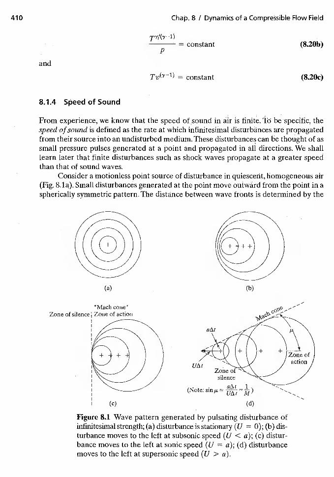
= constant (8.20b)p
From experience, we know that the speed of sound in air is finite. To be specific, thespeedofsound is defined as the rate at which infinitesimal disturbances are propagatedfrom their source into an undisturbed medium.These disturbances can be thought of assmall pressure pulses generated at a point and propagated in all directions. We shalllearn later that finite disturbances such as shock waves propagate at a greater speedthan that of sound waves.
Consider a motionless point source of disturbance in quiescent, homogeneous air(Fig. 8.la). Small disturbances generated at the point move outward from the point in aspherically symmetric pattern. The distance between wave fronts is determined by the
"Mach cone"Zone of silence Zone of action
(d)
Figure 8.1 Wave pattern generated by pulsating disturbance ofinfinitesimal strength; (a) disturbance is stationary (U = 0); (b) dis-turbance moves to the left at subsonic speed (U < a); (c) distur-bance moves to the left at sonic speed (U = a); (d) disturbancemoves to the left at supersonic speed (U > a).
410 Chap. 8 I Dynamics of a Compressible Flow Field
and
8.1.4 Speed of Sound
= constant (8.20c)
(a) (b)
(c)
Zonesilence
aAt 1.(Note:
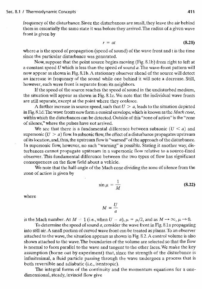
Sec. 8.1 I Thermodynamic Concepts 411
frequency of the disturbance. Since the disturbances are small, they leave the air behindthem in essentially the same state it was before they arrived.The radius of a given wavefront is given by
r = at (8.21)
where a is the speed of propagation (speed of sound) of the wave front and t is the timesince the particular disturbance was generated.
Now, suppose that the point source begins moving (Fig. 8db) from right to left ata constant speed U which is less than the speed of sound a. The wave-front pattern willnow appear as shown in Fig. 8db. A stationary observer ahead of the source will detectan increase in frequency of the sound while one behind it will note a decrease. Still,however, each wave front is separate from its neighbors.
If the speed of the source reaches the speed of sound in the undisturbed medium,the situation will appear as shown in Fig. 8.lc. We note that the individual wave frontsare still separate, except at the point where they coalesce.
A further increase in source speed, such that U > a, leads to the situation depictedin Fig. 8.ld.The wave fronts now form a conical envelope, which is known as the Mach cone,within which the disturbances can be detected. Outside of this "zone of action" is the "zoneof silence," where the pulses have not arrived.
We see that there is a fundamental difference between subsonic (U < a) andsupersonic (U > a) flow. In subsonic flow, the effect of a disturbance propagates upstreamof its location, and, thus, the upstream flow is "warned" of the approach of the disturbance.In supersonic flow, however, no such "warning" is possible. Stating it another way, dis-turbances cannot propagate upstream in a supersonic flow relative to a source-fixedobserver. This fundamental difference between the two types of flow has significantconsequences on the flow field about a vehicle.
We note that the half-angle of the Mach cone dividing the zone of silence from thezone of action is given by
= 1 (8.22)
where
a
is the Mach number. At M = 1 (i.e., when U = a), and as M 00, p. 0.
To determine the speed of sound a, consider the wave front in Fig. 8.1 a propagatinginto still air.A small portion of curved wave front can be treated as planar.To an observerattached to the wave, the situation appears as shown in Fig. 8.2. A control volume is alsoshown attached to the wave. The boundaries of the volume are selected so that the flowis normal to faces parallel to the wave and tangent to the other faces. We make the keyassumption (borne out by experiment) that, since the strength of the disturbance isinfinitesimal, a fluid particle passing through the wave undergoes a process that isboth reversible and adiabatic (i.e., isentropic).
The integral forms of the continuity and the momentum equations for a one-dimensional, steady, inviscid flow give
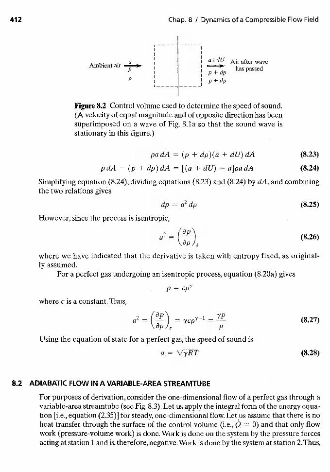
412 Chap. 8 I Dynamics of a Compressible Flow Field
a {a+dU Air after waveAmbient air has passed
I p+dpP p+dp
Figure 8.2 Control volume used to determine the speed of sound.(A velocity of equal magnitude and of opposite direction has beensuperimposed on a wave of Fig. 8.la so that the sound wave isstationary in this figure.)
padA = (p + dp)(a + dU)dA (8.23)
pdA — (p + dp)dA = [(a + dU) — a]padA (8.24)
Simplifying equation (8.24), dividing equations (8.23) and (8.24) by dA, and combiningthe two relations gives
dp = a2 dp (8.25)
However, since the process is isentropic,
a2=
(8.26)S
where we have indicated that the derivative is taken with entropy fixed, as original-ly assumed.
For a perfect gas undergoing an isentropic process, equation (8.20a) gives
p =c is a constant. Thus,
a2 = = (8.27)P
Using the equation of state for a perfect gas, the speed of sound is
a = (8.28)
8.2 ADIABATIC FLOW IN A VARIABLE-AREA STREAMTUBE
For purposes of derivation, consider the one-dimensional flow of a perfect gas through avariable-area streamtube (see Fig. 8.3). Let us apply the integral form of the energy equa-tion [i.e., equation (2.35)} for steady, one-dimensional flow. Let us assume that there is noheat transfer through the surface of the control volume (i.e., Q = 0) and that only flowwork (pressure-volume work) is done. Work is done on the system by the pressure forcesacting at station 1 and is, therefore, negative. Work is done by the system at station 2. Thus,
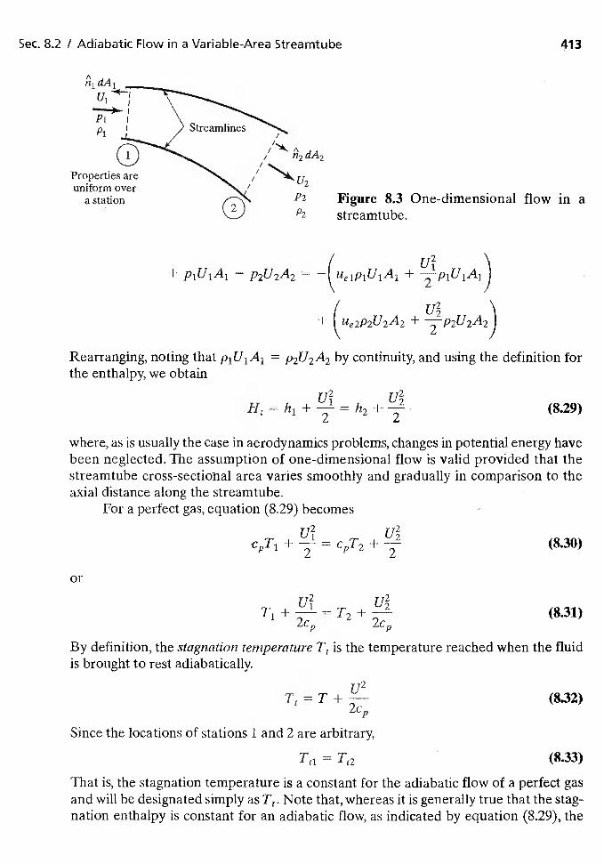
Sec. 8.2 I Adiabatic Flow in a Variab'e-Area Streamtube 413
Figure 8.3 One-dimensional flow in astreamtube.
U2+ p1U1A1 — p2U2A2 = Ue1P1U1A1 +
p1U1A1 = p2U2A2 by continuity, and using the definition forthe enthalpy, we obtain
U2 U2H1 = h1 + = h2 +- (8.29)
where, as is usually the case in aerodynamics problems, changes in potential energy havebeen neglected. The assumption of one-dimensional flow is valid provided that thestreamtube cross-sectional area varies smoothly and gradually in comparison to theaxial distance along the streamtube.
For a perfect gas, equation (8.29) becomes
u2+ = + (8.30)
or
U2 u2(831)
By definition, the stagnation temperature T1 is the temperature reached when the fluidis brought to rest adiabatically.
U2T1=T+— (8.32)
Since the locations of stations 1 and 2 are arbitrary,
T11 = (8.33)
That is, the stagnation temperature is a constant for the adiabatic flow of a perfect gasand will be designated simply as T1, Note that, whereas it is generally true that the stag-nation enthalpy is constant for an adiabatic flow, as indicated by equation (8.29), the
p1
Properties areuniform over
a station P2
p2
414 Chap. 8 I Dynamics of a Compressible Flow Field
stagnation temperature is constant only if the additional condition that is constant(i.e., the gas behaves as a perfect gas) is satisfied.
For any one-dimensional adiabatic flow,
_1+Y'M2 834T — 2[yR/(y 1)]T - 2
Note that we have used the perfect-gas relations that = yR/(y — 1) and that a2 = yRT.It is interesting to note that, when the flow is isentropic, Euler's equation for
one-dimensional, steady flow (i.e., the inviscid-flow momentum equation) gives the sameresult as the energy equation for an adiabatic flow. To see this, let us write equation (3.2)for steady, one-dimensional, inviscid flow:
du dp= — —i-- (8.35a)
fdp c/ + / is du = 0 (8.35b)ip J
Note that for a one-dimensional flow u = U. For an isentropic process (which is ofcourse adiabatic),
Differentiating, substituting the result into equation (8.35b), and integrating, we obtain
y+ = constanty—l 2
Thus,
1 yp U2
_____—
+ = constanty—lp 2
Using the perfect-gas equation of state, we obtain
U2h + = constant
which is equation (8.29).
EXAMPLE 8.1: An indraft, supersonic wind tunnel
We are to design a supersonic wind tunnel using a large vacuum pump todraw air from the ambient atmosphere into our tunnel, as shown in Fig. 8.4.The air is continuously accelerated as it flows through a convergent/divergentnozzle so that flow in the test section is supersonic. If the ambient air is at thestandard sea-level conditions, what is the maximum velocity that we can attainin the test section?
Solution: To calculate this maximum velocity, all we need is the energy equation for asteady, one-dimensional, adiabatic flow. Using equation (8.29), we have

Sec. 8.2 I Adiabatic. Flow in a Variable-Area Streamtube 415
Anibient airat standard 0conditions serves
- Test sectionas tunnelreservoir "Sonic throat"
To vacuum system
Figure 8.4 Indraft, supersonic wind tunnel.
Since the ambient air (i.e., that which serves as the tunnel's "stagnation cham-ber" or "reservoir") is at rest, U1 = 0. The maximum velocity in the test sec-tion occurs when h2 = 0 (i.e., when the flow expands until the statictemperature in the test section is zero).
(1004.7)288.15J/kg
U2 = 760.9 rn/s
Of course,we realize that this limit is physically unattainable, since the gaswould liquefy first. However, it does represent an upper limit for conceptualconsiderations.
EXAMPLE 8.2: A simple model for the Shuttle Orbiter flow field
During a nominal reentry trajectory, the Space Shuttle Orbiter flies at 3964ft/s at an altitude of 100,000 ft. The corresponding conditions at the stagna-tiÔn point (point 2 Fig. 8.5) are P2 = 490.2 lbf/ft2 and T2 = 1716.0°R. Thestatic pressures for two nearby locations (points 3 and 4 of Fig. 8.5) arep3 = 259.0 lbf/ft2 and = 147.1 lbf/ft2. All three points are outside theboundary layer. What ate the local static temperature, the local velocity, andthe local Mach number at points 3 and 4?
Solution: At these conditicins, the air can be assumed to behave approximately as aperfect gas. Furthermore, since all three points are outside the boundarylayer and dowhstream of the bow shock wave, we will assume that the flowexpands isentropically frOm point 2 to point 3 and then to point 4. (Notethat because the shock wave is curved, the entropy will vary through theshock layer. For a further discussion of the rotational flow downstream ofa- curved shock wave, refer to Chapter 12. Thus, validity of the assumptionthat the expansion is isentropic should be verified for a given application.)
For an isentropic process, we can use equation (8.20b) to relate thetemperature ratio to the pressure ratio between two points. Thus,
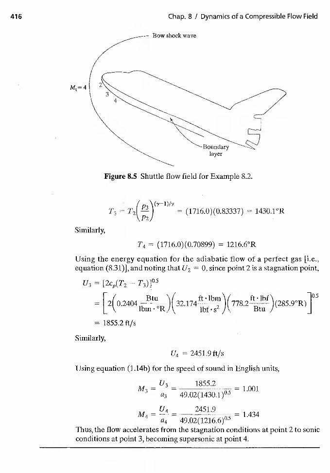
416 Chap. 8 / Dynamics of a Compressible Flow Field
Figure 8.5 Shuttle flow field for Example 8.2.
Similarly,
T3 = (1716.0)(O.83337) = 1430.1°R
= (1716.0)(0.70899) = 1216.6°R
Using the energy equation for the adiabatic flow of a perfect gas [i.e.,equation (8.31)], and noting that U2 = 0, since point 2 is a stagnation point,
U3 = — T3)]°5
Btu= [2(0.2404
ibm °R)(32.174
Btu /
______
ft lbm\ (778.2 ft lbf\28590R)j
= 1855.2 ft/s
U4 2451.9 ft/s
Similarly,
Using equation (1.14b) for the speed of sound in English units,
= U3 1855.2= 1.001
a3
U4 = 2451.9= 1.434
a4
Thus, the flow accelerates from the stagnation conditions at point 2 to sonicconditions at point 3, becoming supersonic at point 4.
Bow shock wave
layer
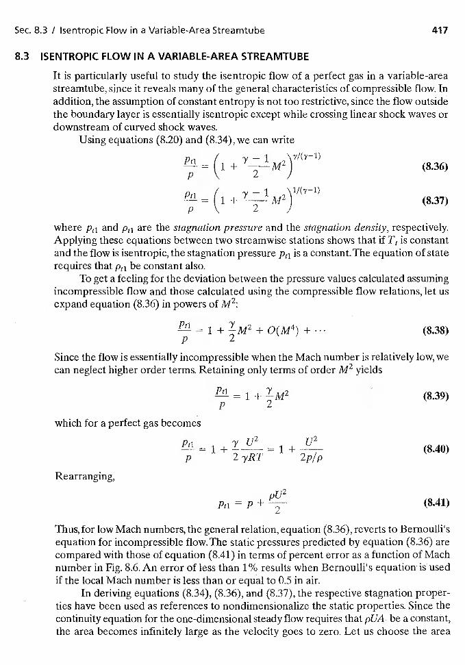
Sec. 83 / isentropic Flow in a Variable-Area Streamtube 417
8.3 ISENTROPIC FLOW IN A VARIABLE-AREA STREAMTUBE
It is particularly useful to study the isentropic flow of a perfect gas in a variable-areastreamtube, since it reveals many of the general characteristics of compressible flow. Inaddition, the assumption of constant entropy is not too restrictive, since the flow outsidethe boundary layer is essentially isentropic except while crossing linear shock waves ordownstream of curved shock waves.
Using equations (8.20) and (8.34), we can write
— 1(i +2
M2) (8.36)
/ 1ivi2) (8.37)
p 2 jwhere Pti and Pti are the stagnation pressure and the stagnation density, respectively.Applying these equations between two streamwise stations shows that if T1 is constantand the flow is isentropic, the stagnation pressure Pti is a constant. The equation of staterequires that Pti be constant also.
To get a feeling for the deviation between the pressure values calculated assumingincompressible flow and those calculated using the compressible flow relations, let usexpand equation (8.36) in powers of M2:
1 + 1M2 + 0(M4) + (8.38)p 2
Since the flow is essentially incompressible when the Mach number is relatively low, wecan neglect higher order terms. Retaining only terms of order M2 yields
I + (8.39)p 2
which for a perfect gas becomes
= + y u2= 1
+ U2(8.40)
p 2yRT 2p/p
Rearranging,
Pri =+
(8.41)
Thus, for low Mach numbers, the general relation, equation (8.36), reverts to Bernoulli'sequation for incompressible flow. The static pressures predicted by equation (8.36) arecompared with those of equation (8.41) in terms of percent error as a function of Machnumber in Fig. 8.6. An error of less than 1% results when Bernoulli's equation isusedif the local Mach number is less than or equal to 0.5 in air.
In deriving equations (8.34), (8.36), and (8.37), the respective stagnation proper-ties have been used as references to nondimensionalize the static properties. Since thecontinuity equation for the one-dimensional steady flow requires that pUA be a constant,the area becomes infinitely large as the velocity goes to zero. Let us choose the area
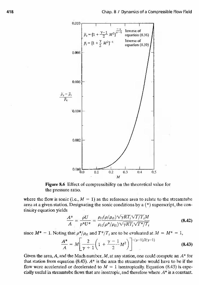
PC — Pa
PC
since M* = 1. Noting that p*/ptl and are to be evaluated at M = M* = 1,
+ 7 1M2)](Y)/(7) (8.43)
Given the area, A, and the Mach number, M, at any station, one could compute an A* forthat station from equation (8.43). A* is the area the streamtube would have to be if theflow were accelerated or decelerated to = I isentropically. Equation (8.43) is espe-daily useful in streamtube flows that are isentropic, and therefore where A* is a constant.
418 Chap. 8 I Dynamics of a Compressible Flow Field
M
Figure 8.6 Effect of compressibility on the theoretical value forthe pressure ratio.
where the flow is sonic (i.e., M = 1): as the reference area to relate to the streamtubearea at a given station. Designating the sonic conditions by a (*) superscript, the con-tinüity equation yields
A* pUA p*U* ptl(p*/ptl)
(8.42)
MA {1 + [(y
— —2 I'ti
'\A)max — R + 1)
Sec. 8.3 / Isentropic Flow in a Variable-Area Streamtube 419
In order to aid in the solution of isentropic flow problems, the temperature ratio[equation (8.34)], the pressure ratio [equation (8.36)], the density ratio [equation (8.37)],and the area ratio [equation (8.43)] are presented as a function of the Mach number inTable 8.1. A more complete tabulation of these data is given in Ames Research CenterStaff (1953). The results of Table 8.1 are summarized in Fig. 8.7.
In order to determine the mass-flow rate in a streamtube,
th = pUA =\PriJ v
(8.44)
Thus, the mass-flow rate is proportional to the stagnation pressure and inversely pro-portional to the square root of the stagnation temperature. To find the condition of max-imum flow per unit area, one could compute the derivative of (th/A) as given byequation (8.44) with respect to Mach number and set the derivative equal to zero. At thiscondition, one would find that M = 1. Thus, setting M = 1 in equation (8.44) yields
The maximum flow rate per unit area occurs where the cross-section area is a mini-mum (designated A*), where the Mach number is one. Thus, the maximum flow rateper unit area occurs at the sonic throat when the flow is choked.
(8.45)
M
Figure 8.7 Property variations as functions of Mach number forisentropic flow for 'y = 1.4.
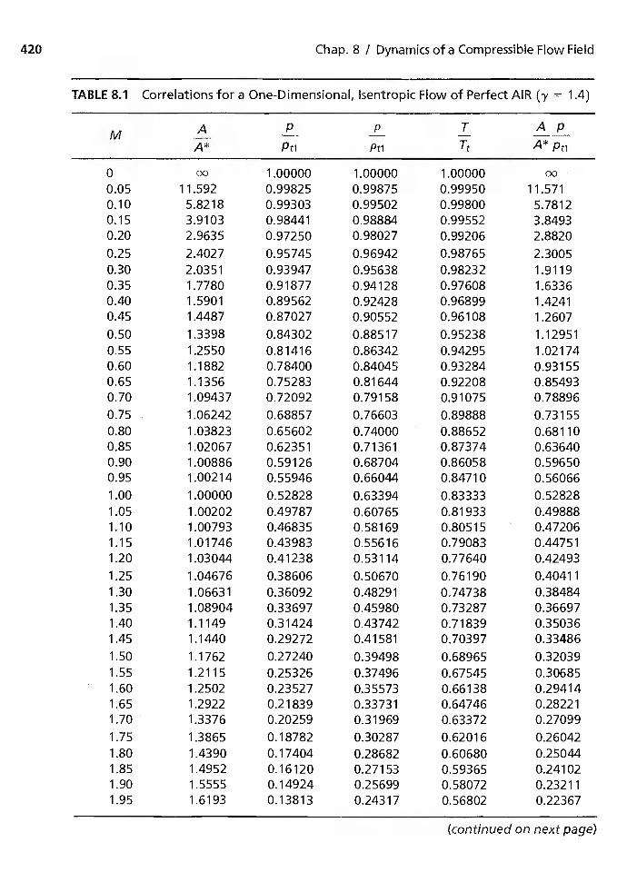
420 Chap. 8 / Dynamics of a Compressible Flow Field
TABLE 8.1 Correlations for a One-Dimensional, Isentropic Flow of Perfect AIR (y 1.4)
M AA*
P
Pti
p
Pti
T ApA* Pti
o 00 1.00000 1.00000 1.00000 00
0.05 11.592 0.99825 0.99875 0.99950 11.5710.10 5.8218 0.99303 0.99502 0.99800 5.78120.15 3,9103 0.98441 0.98884 0.99552 3.84930.20 2.9635 0.97250 0.98027 0.99206 2.88200.25 2.4027 0.95745 0.96942 0.98765 2.30050.30 2.0351 0.93947 0.95638 0.98232 1.91190.35 1.7780 0.91877 0.94128 0.97608 1.63360.40 1.5901 0.89562 0.92428 0.96899 1.42410.45 1,4487 0.87027 0.90552 0.96108 1.2607
0.50 1.3398 0.84302 0.88517 0.95238 1.129510.55 1.2550 0.81416 0.86342 0.94295 1.021740.60 11882 0.78400 0.84045 0.93284 0.931550.65 1.1356 0.75283 0.81644 0.92208 0.854930.70 1.09437 0.72092 0.79158 0.91075 0.788960.75 1.06242 0.68857 0.76603 0.89888 0.731550.80 1.03823 0.65602 0.74000 0.88652 0.681100.85 1.02067 0.62351 0.71361 0.87374 0.636400.90 1.00886 0.59126 0.68704 0.86058 0.596500.95 1.00214 0.55946 0.66044 0.84710 0.56066
1.00 1.00000 0.52828 0.63394 0.83333 0.528281.05 1.00202 0.49787 0.60765 0.81933 0.498881.10 1.00793 0.46835 0.58169 0.80515 0.472061.15 1.01746 0.43983 0.55616 0.79083 0.44751
1.20 1.03044 0.41238 0.53114 0.77640 0.42493
1.25 1.04676 0.38606 0.50670 0.76190 0.40411
1.30 1.06631 0.36092 0.48291 0.74738 0.384841.35 1.08904 0.33697 0.45980 0.73287 0.36697
1.40 1.1149 0.31424 0.43742 0,71839 0.350361.45 1.1440 0.29272 0.41581 0.70397 0.33486
1.50 1.1762 0.27240 0.39498 0.68965 0.320391.55 1.2115 0.25326 0.37496 0.67545 0.306851.60 1.2502 0.23527 0.35573 0.66138 0.294141.65 1.2922 0.21839 0.33731 0.64746 0.282211.70 1.3376 0.20259 0.31969 0.63372 0.27099
1.75 1.3865 0.18782 0.30287 0.62016 0.260421.80 1.4390 0.17404 0.28682 0.60680 0.250441.85 1.4952 0.16120 0.27153 0.59365 0.241021.90 1.5555 0.14924 0.25699 0.58072 0.232111.95 1.6193 0.13813 0.24317 0.56802 0.22367
(continued on next page)
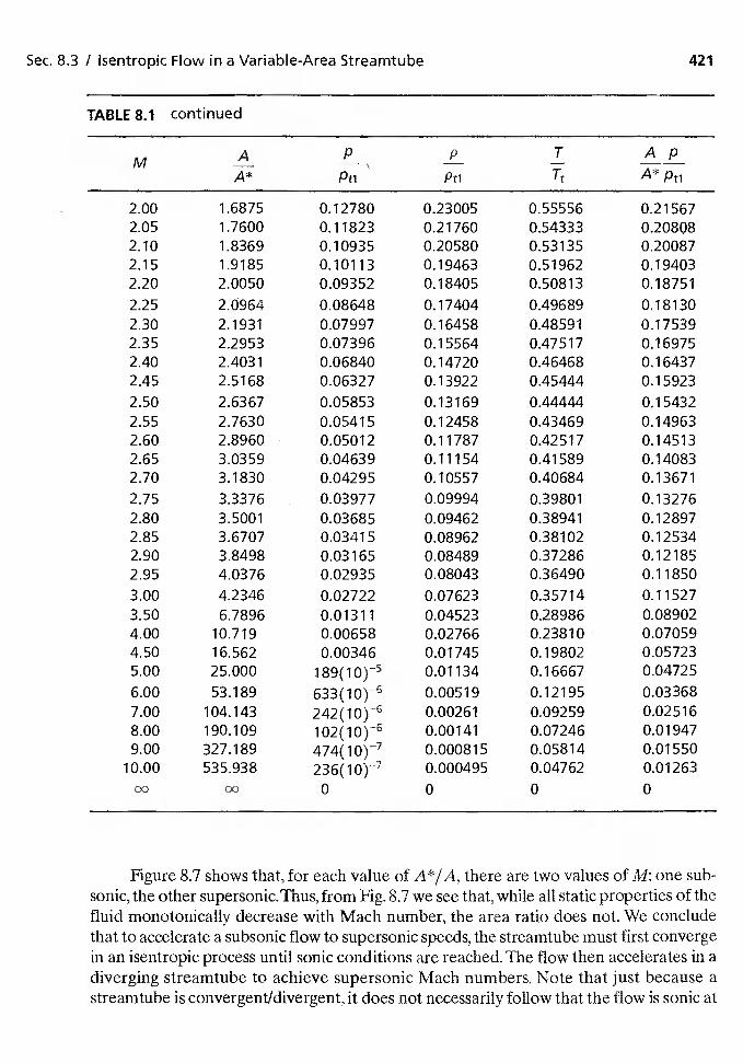
Sec. 8.3 / Isentropic Flow in a Variable-Area Streamtube 421
TABLE 8.1 continued
M AA*
P
Pti
p
Pti
T ApA* Pti
2.00 1.6875 0.12780 0.23005 0.55556 0.215672.05 1.7600 0.11823 0.21760 0.54333 0.208082.10 1.8369 0.10935 0.20580 0.53135 0.200872.15 1.9185 0.10113 0.19463 0.51962 0.194032.20 2.0050 0.09352 0.18405 0.50813 0.18751
2.25 2.0964 0.08648 0.17404 0.49689 0.181302.30 2.1931 0.07997 0.16458 0.48591 0.175392.35 2.2953 0.07396 0.15564 0.47517 0.169752.40 2.4031 0.06840 0.14720 0.46468 0.164372.45 2.5168 0.06327 0.13922 0.45444 0.15923
2.50 2.6367 0.05853 0.13169 0.44444 0.154322.55 2.7630 0.05415 0.12458 0.43469 0.149632.60 2.8960 0.05012 0.11787 0.42517 0.145132.65 3.0359 0.04639 0.11154 0.41589 0.140832.70 3.1830 0.04295 0.10557 0.40684 0.13671
2.75 3.3376 0.03977 0.09994 0.39801 0.132762.80 3.5001 0.03685 0.09462 0.38941 0.12897
2.85 3.6707 0.03415 0.08962 0.38102 0.125342.90 3.8498 0.03165 0.08489 0.37286 0.12185
2.95 4.0376 0.02935 0.08043 0.36490 0.11850
3.00 4.2346 0.02722 0.07623 0.35714 0.115273.50 6.7896 0.01311 0.04523 0.28986 0.089024.00 10.719 0.00658 0.02766 0.23810 0.07059
4.50 16.562 0.00346 0.01745 0.19802 0.057235.00 25.000 0.01134 0.16667 0.04725
6.00 53.189 633(10)_6 0.00519 0.12195 0.033687.00 104.143 242(10)6 0.00261 0.09259 0,025168.00 190.109 0.00141 0.07246 0.019479.00 327.189 474(10y7 0.000815 0.05814 0.01550
10.00 535.938 236(10)-v 0.000495 0.04762 0.0126300 00 0 0 0 0
Figure 8.7 shows that, for each value of A*/A, there are two values of M: one sub-sonic, the other supersonic. Thus, from Fig. 8.7 we see that, while all static properties of thefluid monotonically decrease with Mach number, the area ratio does not. We concludethat to accelerate a subsonic flow to supersonic speeds, the streamtube must first convergein an isentropic process until sonic conditions are reached. The flow then accelerates in adiverging streamtube to achieve supersonic Mach numbers. Note that just because astreamtube is convergent/divergent, it does not necessarily follow that the flow is sonic at
422 Chap. 8 / Dynamics of a Compressible Flow Field
the narrowest cross section (or throat).The actual flow depends on the pressure distribu-tion as well as the geometry of the streamtube. However, if the Mach number is to beunity anywhere in the streamtube, it must be so at the throat.
For certain calculations (e.g., finding the true airspeed from Mach number andstagnation pressure) the ratio 0.5 is useful.
0.5pU2 iyp U2 — yM2 p(8 46)
Pri Pti — 2 Pti yRT — 2 Pti
Thus,
0.5pU2 7M2 / — 1= (\i + M2) (847)
Pti 2 2
The ratio of the local speed of sound to the speed of sound at the stagnation conditions is
==
= +2
lM2) (8.48)
Note: The nomenclature used herein anticipates the discussion of shock waves. Sincethe stagnation pressure varies across a shock wave, the subscript ti has been used todesignate stagnation properties evaluated upstream of a shock wave (which correspondto the free-stream values in a flow with a single shock wave). Since the stagnation tem-perature is constant across a shock wave (for perfect-gas flows), it is designated by thesimple subscript t.
8.4 CHARACTERISTIC EQUATIONS AND PRANDTL-MEYER FLOWS
Consider a two-dimensional flow around a slender airfoil shape. The deflection of thestreamlines as flow encounters the airfoil are sufficiently small that shock waves are not gen-erated. Thus, the flow may be considered as isentropic (excluding the boundary layer, ofcourse). For the development of the equations for a more general flow, refer to Hayes andProbstein (1966). For the present type of flow, the equations of motion in a natural (orstreamline) coordinate system, as shown in Fig. 8.8, are as follows: the continuity equation,
+ pU— = 0 (8.49)as
the s-momentum equation,
(8.59)
and the n-momentum equation,
+ = 0 (8.51)as an
Since the flow is isentropic, the energy equation provides no unique information and is,therefore, not used. However, since the flow is isentropic, the change in pressure with re-
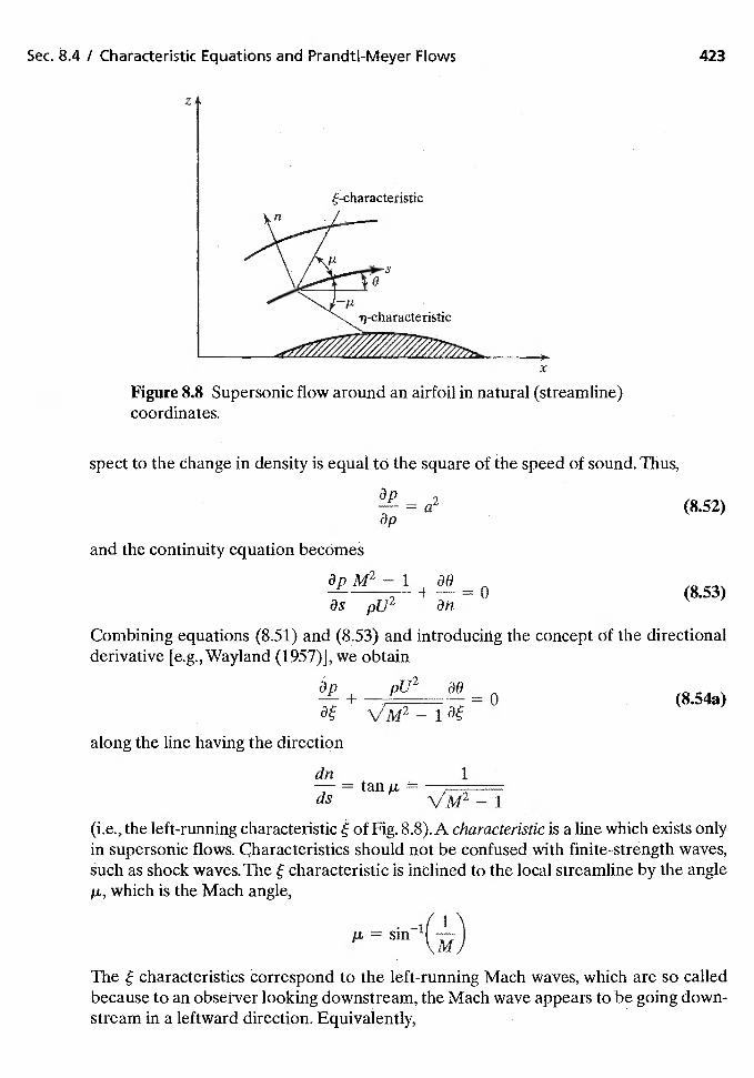
2—=a'3p
dn 1= tan p =
ds \/M2—1(i.e., the left-running characteristic of Fig. 8.8). A characteristic is a line which exists onlyin supersonic flow& characteristics should not be confused with finite-strength waves,such as shock waves. The characteristic is inclined to the local streamline by the anglep, which is the Mach angle,
JL =
The characteristics correspond to the left-running Mach waves, which are so calledbeause to an observer looking downstream, the Mach wave appears to be going down-stream in a leftward direction. Equivalently,
Sec. 8.4 I Characteristic Equations and Prandtl-Meyer Flows
z
e-characteristic
423
Figure 8.8 Supersonic flow around an airfoil in natural (streamline)coordinates.
spect to the change in density is equal to the square of the speed of sound. Thus,
(8.52)
and the continuity equation becOmes
äpM2—1300(8.53)
as PU
Combining equations (8.51) and (8.53) and introducing the concept of the directionalderivative [e.g.,Wayland (1957)], we obtain
+ pu2 30= o (8.54a)
along the line having the direction
x
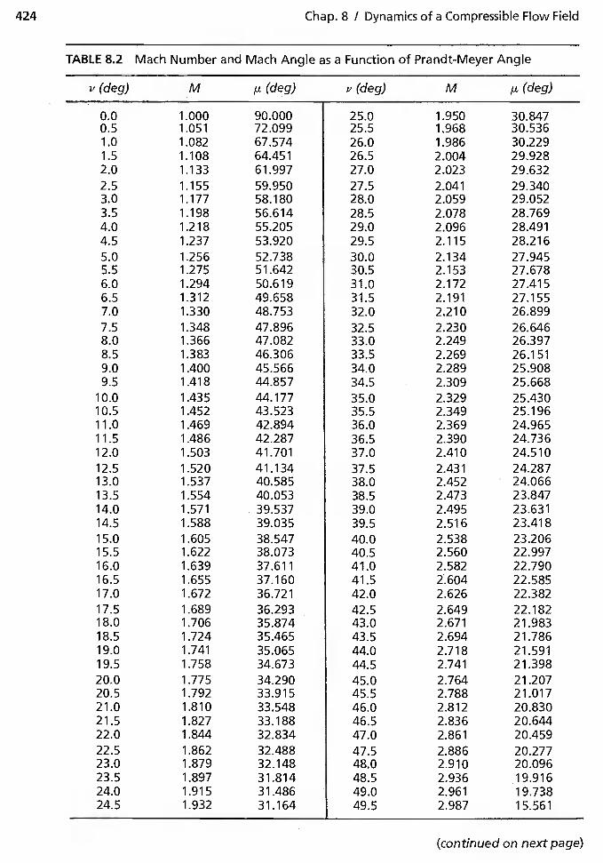
424 Chap. 8 / Dynamics of a Compressible Flow Field
TABLE 8.2 Mach Number and Mach Angle as a Function of Prandt-Meyer Angle
v (deg) M (deg) v ('deg,) M p. (deg)
0.0 1.000 90.000 25.0 1.950 30.8470.5 1.051 72.099 25.5 1.968 30.5361.0 1.082 67.574 26.0 1.986 30.2291.5 1.108 64.451 26.5 2.004 29.9282.0 1.133 61.997 27.0 2.023 29.6322.5 1.155 59.950 27.5 2.041 29.3403.0 1.177 58.180 28.0 2.059 29.0523.5 1.198 56.614 28.5 2.078 28.7694.0 1.218 55.205 29.0 2.096 28.4914.5 1.237 53.920 29.5 2.115 28.2165.0 1.256 52.738 30.0 2.134 27.9455.5 1.275 51.642 30.5 2.153 27.6786.0 1.294 50.619 31.0 2.172 27.4156.5 1.312 49.658 31.5 2.191 27.1557.0 1.330 48.753 32.0 2.210 26.8997.5 1.348 47.896 32.5 2.230 26.6468.0 1.366 47.082 33.0 2.249 26.3978.5 1.383 46.306 33.5 2.269 26.1519.0 1.400 45.566 34.0 2.289 25.9089.5 1.418 44.857 34.5 2.309 25.668
10.0 1.435 44.177 35.0 2.329 25.43010.5 1.452 43.523 35.5 2.349 25.19611.0 1.469 42.894 36.0 2.369 24.96511.5 1.486 42.287 36.5 2.390 24.73612.0 1.503 41.701 37.0 2.410 24.51012.5 1.520 41.134 37.5 2.431 24.28713.0 1.537 40.585 38.0 2.452 24.06613.5 1.554 40.053 38.5 2.473 23.84714.0 1.571 39.537 39.0 2.495 23.63114.5 1.588 39.035 39.5 2.516 23.41815.0 1.605 38.547 40.0 2.538 23.20615.5 1.622 38.073 40.5 2.560 22.99716.0 1.639 37.611 41.0 2.582 22.79016.5 1.655 37.160 41.5 22.58517.0 1.672 36.721 42.0 2.626 22.38217.5 1.689 36.293 42.5 2.649 22.18218.0 1.706 35.874 43.0 2.671 21.98318.5 1.724 35.465 43.5 2.694 21.78619.0 1.741 35.065 44.0 2.7 18 21.59119.5 1.758 34.673 44.5 2.741 21.39820.0 1.775 34.290 45.0 2.764 21.20720.5 1.792 33.915 45.5 2.788 21.01721.0 1.810 33.548 46.0 2.812 20.83021.5 1.827 33.188 46.5 2.836 20.64422.0 1.844 32.834 47.0 2.861 20.45922.5 1.862 32.488 47.5 2.886 20.27723.0 1.879 32.148 48.0 2.910 20.09623.5 1.897 31.814 48.5 2.936 19.91624.0 1.915 31.486 49.0 2.961 19.73824.5 1.932 31.164 49.5 2.987 15.561
(continued on next page)
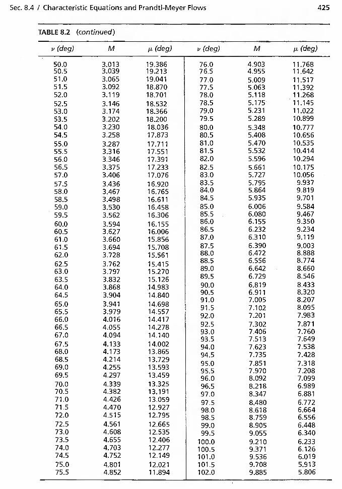
Sec. 8.4 I Characteristic Equations and Prandtl-Meyer F'ows 425
TABLE 8.2 (continued)
v (deg) M p. (deg) v (deg) M p. (deg) -
50.0 3.013 19.386 76.0 4.903 11.76850.5 3.039 19.213 76.5 4.955 11.64251.0 3.065 19.041 77.0 5.009 11.51751.5 3.092 18.870 77.5 5.063 11.39252.0 3.119 18.701 78.0 5.118 11.26852.5 3.146 18.532 78.5 5.175 11.14553.0 3.174 18,366 79.0 5.231 11.02253.5 3.202 18.200 79.5 5.289 10.89954.0 3.230 18.036 80.0 5.348 10.77754.5 3.258 17.873 80.5 5.408 10.65655.0 3.287 17.711 81.0 5.470 10.53555.5 3.316 17.551 81.5 5.532 10.41456.0 3.346 17.391 82.0 5.596 10.29456.5 3.375 17.233 82.5 5.661 10.17557.0 3.406 17.076 83.0 5.727 10.05657.5 3.436 16.920 83.5 5.795 9.93758.0 3.467 16.765 84.0 5.864 9.81958.5 3.498 16.611 84.5 5.935 9.701
59.0 3.530 16.458 85.0 6.006 9.58459.5 3.562 16.306 85.5 6.080 9.467
60.0 3.594 16.155 86.0 6.155 9.350
60.5 3.627 16.006 86,5 6.232 9.234
61.0 3.660 15.856 87.0 6.310 9.119
61.5 3.694 15.708 87.5 6.390 9.00362.0 3.728 15.561 88.0 6.472 8.888
62 5 3 762 15 415 88.5 6.556 8.774
630 3797 15270 89.0 6.642 8.660
63.5 3.832 15.126 89.5 6.729 8.546
64.0 3.868 14.983 90.0 6.819 8.433
645 3904 14840 90.5 6.911 8.320
650 3941 1469891.0 7.005 8.207
65.5 3.979 14.557 91.5 7.102 8.095
66.0 4.016 14.417 92.0 7.201 .983
665 4055 14278 92.5 7.302 7.871
67.5 4.133 14.002 94:0 7.623 7:53868.0 4.173 13.865 945 7735 742868.5 4.214 13.729
69.5 4.297 13.459 96:0 8:092 7:09970.0 4.339 13.325 96.5 8.218 6.98970.5 4.382 13.191 97.0 8.347 6.88171.0 4.426 13.059 97 5 8.480 6.77271.5 4.470 12.927 980 8618 666472.0 4.515 12.795 98:5 8.759 6.55672.5 4.561 12.665 99.0 8.905 6.44873.0 4.608 12.535 99.5 9.055 6.34073.5 4.655 12.406 100.0 9.210 6.23374.0 4.703 12.277 100.5 9.371 6.12674.5 4.752 12.149 101.0 9.536 6.01975.0 4.801 12.021 101.5 9.708 5.91375.5 4.852 11.894 102.0 9.885 5.806
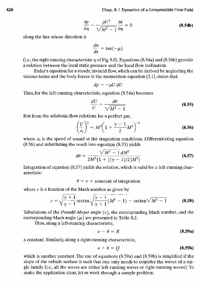
426 Chap. 8 / Dynamics of a Compressible Flow Field
2
an
along the line whose direction is
dn=
(i.e., the right-running characteristic of Fig. 8.8). Equations (8.54a) and (8.54b) providea relation between the local static pressure and the local flow inclination.
Euler's equation for a steady, inviscid flow, which can be derived by neglecting theviscous terms and the body forces in the momentum equation (3.1), states that
dp = —pUdU
Thus, for the left-running characteristic, equation (8.54a) becomes
dU dO
U VM2_lBut from the adiabatic-flow relations for a perfect gas,
(U)2= M2(1 + lM2) (8.56)
where is the speed of sound at the stagnation conditions. Differentiating equation(8.56) and substituting the result into equation (8.55) yields
dO= \/M2 — 1 dM2
(8.57)2M2{1 + [(y — 1)/2]M2}
Integration of equation (8.57) yields the relation, which is valid for a left-running char-acteristic:
0 = v + constant of integration
where i-' is a function of the Mach number as given by
[y+1 Iy—ip = arctan I (M2 — 1) — arctanVM2 — 1 (8.58)
Vy—1 Vy+1Tabulations of the Prandtl-Meyer angle (v), the corresponding Mach number, and thecorresponding Mach angle (ps) are presented in Table 8.2.
Thus, along a left-running characteristic,
v — 0= R (8.59a)
a constant. Similarly, along a right-running characteristic,
v+0=Q (8.59b)
which is another constant. The use of equations (8.59a) and (8.59b) is simplified if theslope of the vehicle surface is such that one only needs to consider the waves of a sin-gle family (i.e., all the waves are either left-running waves or right-running waves). Tomake the application clear, let us work through a sample problem
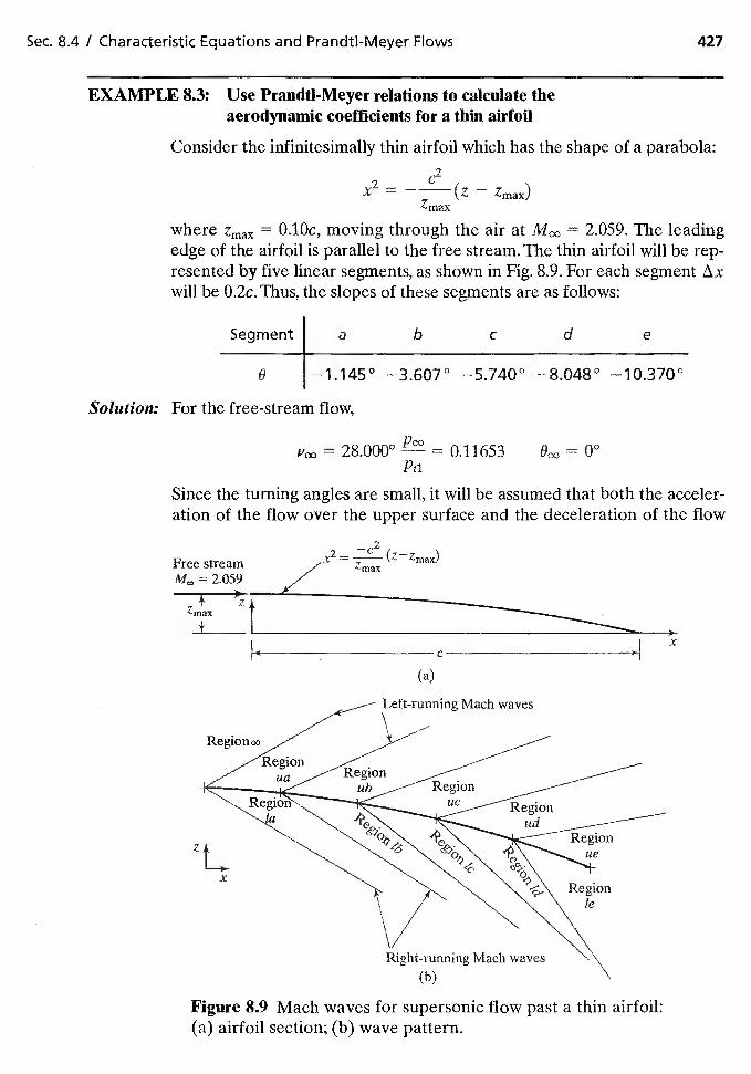
Sec. 8.4 / Characteristic Equations and Prandti-Meyer Flows 427
EXAMPLE 8.3: Use Prandtl-Meyer relations to calculate theaerodynamic coefficients for a thin airfoil
Consider the infinitesimally thin airfoil which has the shape of a parabola:
2 Cx —————(z — Zmax)
where = 0.lOc, moving through the air at = 2.059. The leadingedge of the airfoil is parallel to the free stream. The thin airfoil will be rep-resented by five linear segments, as shown in Fig. 8.9. For each segmentwill be 0.2c. Thus, the slopes of these segments are as follows:
For the free-stream flow,
= 0.11653Pu
aUc.3 U
Since the turning angles are small, it will be assumed that both the acceler-ation of the flow over the upper surface and the deceleration of the flow
Free streamM,, = 2.059
4 zZmax
+
2X2 = (ZZmax)
(b)
Figure 8.9 Mach waves for supersonic flow past a thin airfoil:(a) airfoil section; (b) wave pattern.
Segment a b
8
C d e
—1.145° —3.607° —8.048° —10.370°
(a)
Regionco
Left-running Mach waves
Right-running Mach waves
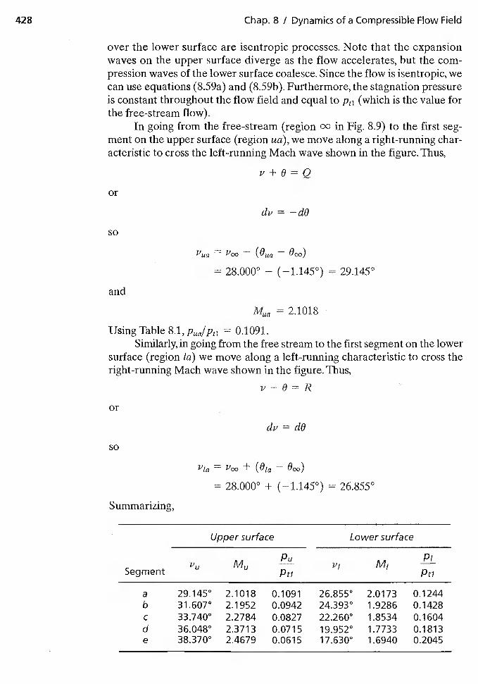
428 Chap. 8 / Dynamics of a Compressible Flow Field
over the lower surface are isentropic processes. Note that the expansionwaves on the upper surface diverge as the flow accelerates, but the com-pression waves of the lower surface coalesce. Since the flow is isentropic, wecan use equations (8.59a) and (8.59b). Furthermore, the stagnation pressureis constant throughout the flow field and equal to Pu (which is the value forthe free-stream flow).
In going from the free-stream (region cc in Fig. 8.9) to the first seg-ment on the upper surface (region ua), we move along a right-running char-acteristic to cross the left-running Mach wave shown in the figure. Thus,
or
= —dO
so
= p00 (Ow, —
= 28.000° — (—1.145°) = 29.145°
and
= 2.1018
Using Table 8.1, = 0,1091.Similarly, in going from the free stream to the first segment on the lower
surface (region la) we move along a left-running characteristic to cross theright-running Mach wave shown in the figure. Thus,
ii-O=Ror
clv = dO
so
1'la = + Oc,o)
= 28.000° + (—1.145°) = 26.855°
Summarizing,
Segment
Upper surface Lower surface
Pu
Ptivj M1
P1
Pti
abc
de
29.145031.607033.740036.048038.370°
2.10182.19522.27842.37132.4679
0.10910.09420.08270.07150.0615
26.855°24.393022.260°19.952°17.630°
2.01731.92861.85341.77331.6940
0.12440.14280.16040.18130.2045
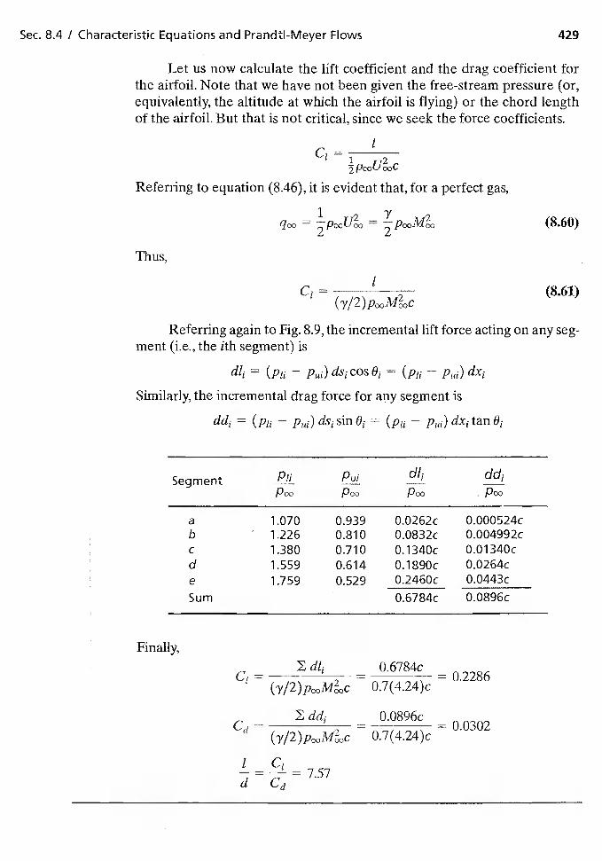
Sec. 8.4 / Characteristic Equations and Prandtl-Meyer Flows 429
Let us now calculate the lift coefficient and the drag coefficient forthe airfoil. Note that we have not been given the free-stream pressure (or,equivalently, the altitude at which the airfoil is flying) or the chord lengthof the airfoil. But that is not critical, since we seek the force coefficients.
1cl=
Referring to equation (8.46), it is evident that, for a perfect gas,
= = (8.60)
Thus,
C1 = (8.61)
Referring again to Fig. 8.9, the incremental lift force acting on any seg-ment (i.e., the ith segment) is
d11 = (Pu — ds, cos 0, = — dx1
Similarly, the incremental drag force for any segment is
dd1 = (Pu — sin 0, = (Pu — dx, tan
SegmentPoo Pco Poo Pco
a 1.070 0.939 O.0262c 0.000524cb 1.226 0.810 O.0832c 0.004992cc 1.380 0.710 0.1340c 0.01340cd 1359 0.614 0.1890c 0.0264ce 1.759 0.529 0.2460c O.0443c
Sum 0.6784c 0.0896c
Finally,d4 0.6784c
C1 = = 0.22860.7(4.24)c
Cddd1 0.0896c= = 0.0302
= 0.7(4.24)c
= 7.57dCd
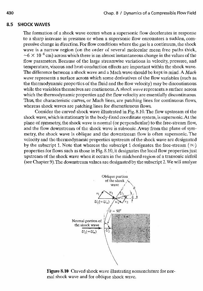
430 Chap. 8 / Dynamics of a Compressible Flow Field
8.5 SHOCK WAVES
The formation of a shock wave occurs when a supersonic flow decelerates in responseto a sharp increase in pressure or when a supersonic flow encounters a sudden, com-pressive change in direction. For flow conditions where the gas is a continuum, the shockwave is a narrow region (on the order of several molecular mean free paths thick,
X 10—6 cm) across which there is an almost instantaneous change in the values of theflow parameters. Because of the large streamwise variations in velocity, pressure, andtemperature, viscous and heat-conduction effects are important within the shock wave.The difference between a shock wave and a Mach wave should be kept in mind. A Machwave represents a surface across which some derivatives of the flow variables (such asthe thermodynamic properties of the fluid and the flow velocity) may be discontinuouswhile the variables themselves are continuous. A shock wave represents a surface acrosswhich the thermodynamic properties and the how velocity are essentially discontinuous.Thus, the characteristic curves, or Mach lines, are patching lines for continuous flows,whereas shock waves are patching lines for discontinuous flows.
Consider the curved shock wave illustrated in Fig. 8.10. The flow upstream of theshock wave, which is stationary in the body-fixed coordinate system, is supersonic. At theplane of symmetry, the shock wave is normal (or perpendicular) to the free-stream flow,and the flow downstream of the shock wave is subsonic. Away from the plane of sym-metry, the shock wave is oblique and the downstream flow is often supersonic. Thevelocity and the thermodynamic properties upstream of the shock wave are designatedby the subscript 1. Note that whereas the subscript 1 designates the free-stream (cc)properties for flows such as those in Fig. 8.10, it designates the local flow properties justupstream of the shock wave when it occurs in the midchord region of a transonic airfoil(see Chapter 9).The downstream values are designated by the subscript 2.We will analyze
Normal portion ofthe shock wave
U1(=
Figure 8.10 Curved shock wave illustrating nomenclature for nor-mal shock wave and for oblique shock wave.
V1
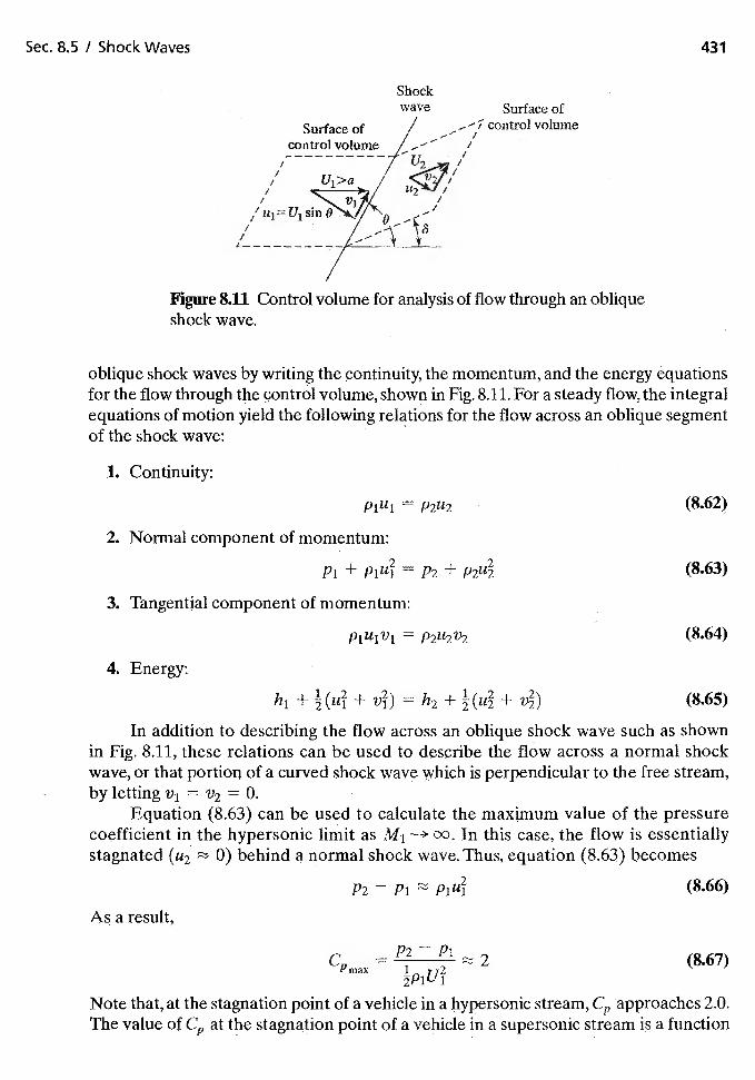
Sec. 8.5 / Shock Waves 431
Shockwave Surface of
control volume
Figure 8.11 Control volume for analysis of flow through an obliqueshock wave.
oblique shock waves by writing the continuity, the momentum, and the energy equationsfor the flow through the ontrol volume, shown in Fig. 8.11. For a steady flow, the integralequations of motion yield the following relations for the flow across an oblique segmentof the shock wave:
1. Continuity:
—
2. Normal component of momentum:
h1 + + = + + (8.65)
In addition to describing the flow across an oblique shock wave such as shownin Fig. 8.11, these relations can be used to describe the flow across a normal shockwave, or that portiorl of a curved shock wave which is perpendicular to the free stream,by letting v1 = 0.
Equation (8.63) can be used to calculate the maximum value of the pressurecoefficient in the hypersonic limit as M1 In this case, the flow is essentiallystagnated (u2 0) behind a normal shock wave. Thus, equation (8.63) becomes
P2 — P1 (8.66)
As a
c P2 — Pi (8.67)Pmax 1
1
Note that, at the stagnation point of a vehicle in a hypersonic stream, approaches 2.0.The value of at the stagnation point of a vehicle in a supersonic stream is a function
Surface ofcontrol volume
Pi + P2 + P2U2
3. Tangential component of momentum:
= P21L2V2
4. Energy:
(8.62)
(8.63)
(8.64)
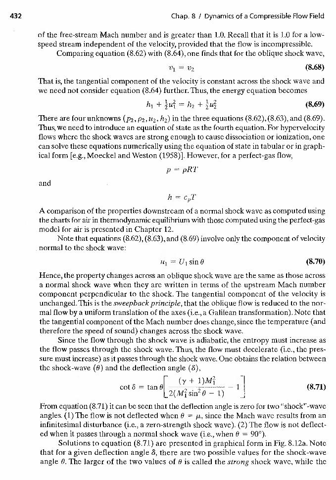
432 Chap. 8 / Dynamics of a Compressible Flow Field
of the free-stream Mach number and is greater than 1.0. Recall that it is 1.0 for a low-speed stream independent of the velocity, provided that the flow is incompressible.
Comparing equation (8.62) with (8.64), one finds that for the oblique shock wave,
= V2 (8.68)
That is, the tangential component of the velocity is constant across the shock wave andwe need not consider equation (8.64) further. Thus, the energy equation becomes
h1 + = h2 + (8.69)
There are four unknowns (p2. P2, u2, h2) in the three equations (8.62), (8.63), and (8.69).Thus, we need to introduce an equation of state as the fourth equation. For hypervelocityflows where the shock waves are strong enough to cause dissociation or ionization, onecan solve these equations numerically using the equation of state in tabular or in graph-ical form [e.g., Moeckel and Weston (1958)]. However, for a perfect-gas flow,
p=pRTand
A comparison of the properties downstream of a normal shock wave as computed usingthe charts for air in thermodynamic equilibrium with those computed using the perfect-gasmodel for air is presented in Chapter 12.
Note that equations (8.62), (8.63), and (8.69) involve only the component of velocitynormal to the shock wave:
= U1 sin 0 (8.70)
Hence, the property changes across an oblique shock wave are the same as those acrossa normal shock wave when they are written in terms of the upstream Mach numbercomponent perpendicular to the shock. The tangential component of the velocity isunchanged. This is the sweep back principle, that the oblique flow is reduced to the nor-mal flow by a uniform translation of the axes (i.e., a Galilean transformation). Note thatthe tangential component of the Mach number does change, since the temperature (andtherefore the speed of sound) changes across the shock wave.
Since the flow through the shock wave is adiabatic, the entropy must increase asthe flow passes through the shock wave. Thus, the flow must decelerate (i.e., the pres-sure must increase) as it passes through the shock wave. One obtains the relation betweenthe shock-wave (0) and the deflection angle (8),
[ 11 I (8.71)
— 1) JFrom equation (8.71) it can be seen that the deflection angle is zero for two "shock"-waveangles. (1) The flow is not deflected when 0 = since the Mach wave results from aninfinitesimal disturbance (i.e., a zero-strength shock wave). (2) The flow is not deflect-ed when it passes through a normal shock wave (i.e., when 0 = 90°).
Solutions to equation (8.71) are presented in graphical form in Fig. 8.12a. Notethat for a given deflection angle 6, there are two possible values for the shock-waveangle 8. The larger of the two values of 0 is called the strong shock wave, while the
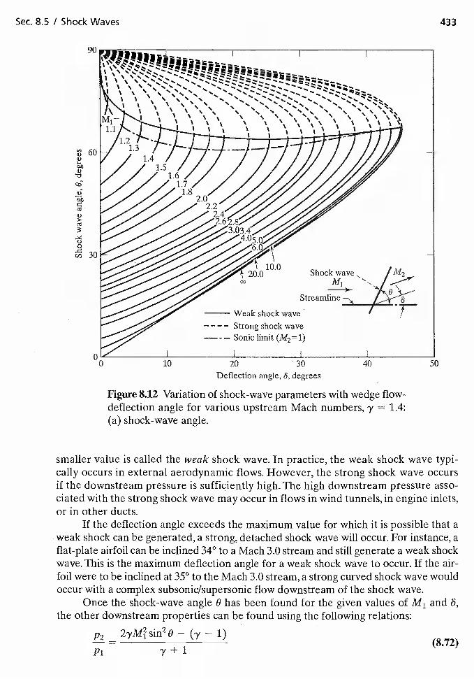
Sec. 8.5 I Shock Waves 433
Figure 8.12 Variation of shock-wave parameters with wedge flow-deflection angle for various upstream Mach numbers, y 1.4:(a) shock-wave angle.
smaller value is called the weak shock wave, In practice, the weak shock wave typi-cally occurs in external aerodynamic flows. However, the strong shock wave occursif the downstream pressure is sufficiently high. The high downstream pressure asso-ciated with the strong shock wave may occur in flows in wind tunnels, in engine inlets,or in other ducts.
If the deflection angle exceeds the maximum value for which it is possible that aweak shock can be generated, a strong, detached shock wave will occur. For instance, aflat-plate airfoil can be inclined 34° to a Mach 3.0 stream and still generate a weak shockwave. This is the maximum deflection angle for a weak shock wave to occur. If the air-foil were to be inclined at 35° to the Mach 3.0 stream, a strong curved shock wave wouldoccur with a complex subsonic/supersonic flow downstream of the shock wave.
Once the shock-wave angle 0 has been found for the given values of M1 and 6,the other downstream properties can be found using the following relations:
P2 = sin2 0 — ('y 1)(8.72)
Pi y+1
a)a)I-,
'a:;
a)
a)
0CO 30
Deflection angle, degrees
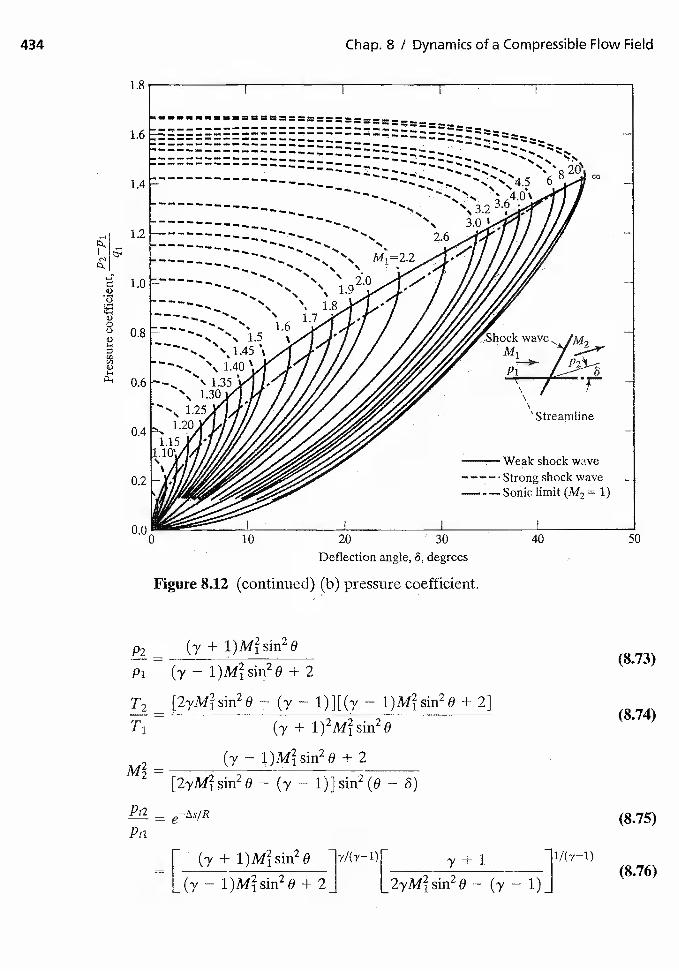
4)U
aU4)
4)
Deflection angle, 6, degrees
Figure 8.12 (continued) (b) pressure coefficient.
('y +
— + 2
— (y — l)][('y — + 2]
(y +
(y — + 2
— ('y — 1)]sin2(O 6)
434
1.8
1.6
Chap. 8 / Dynamics of a Compressible Flow Field
1.2
— — — —
2.6
1.0
cc
M=2.2.-—,..
i1.8
0.81.6
1.5'\1.4
- —1.40
—'S
t0.6-—-.5.
'S
1.
1.
0.2
Weak shock wave— — — —. Strong shock wave— - — Sonic limit (M2 = 1)
20 30 50
P2
P1
T2
(8.73)
(8.74)
(8.75)
(8.76)
=
— [ (y + 1Y/(7_1)[ y + :1
[(,y — + 2J — (y — 1)]
Sec. 8.5 / Shock Waves 435
E
I
and
Deflection angle, 8, degrees
Figure 8.12 (continued) (c) downstream Mach number.
The pressure coefficient is presented in Fig. 8.12b as a function of 6 and M1 . Equation (8.77)is consistent with equation (8.67) for a normal shock since y —*1 as M1 00 due to thedissociation of molecules in the air at high Mach numbers.The values for many of these ra-tios are presented for a normal shock wave in Table 8.3 and in Fig. 8.13.The values for thepressure ratios, the density ratios, and the temperature ratios for an oblique shock wavecan be read from Table 8.3 provided that M1 sin 0 is used instead of M1 in the first column.Note that since it is the tangential component of the velocity which is unchanged and notthe tangential component of the Mach number, we cannot use Table 8.3 to calculate the down-stream Mach number. The downstream Mach number is presented in Fig. 8,12c as a func-
/ /, , / /, / ,
P2P1cpsin 0 — 1)
+(8.77)
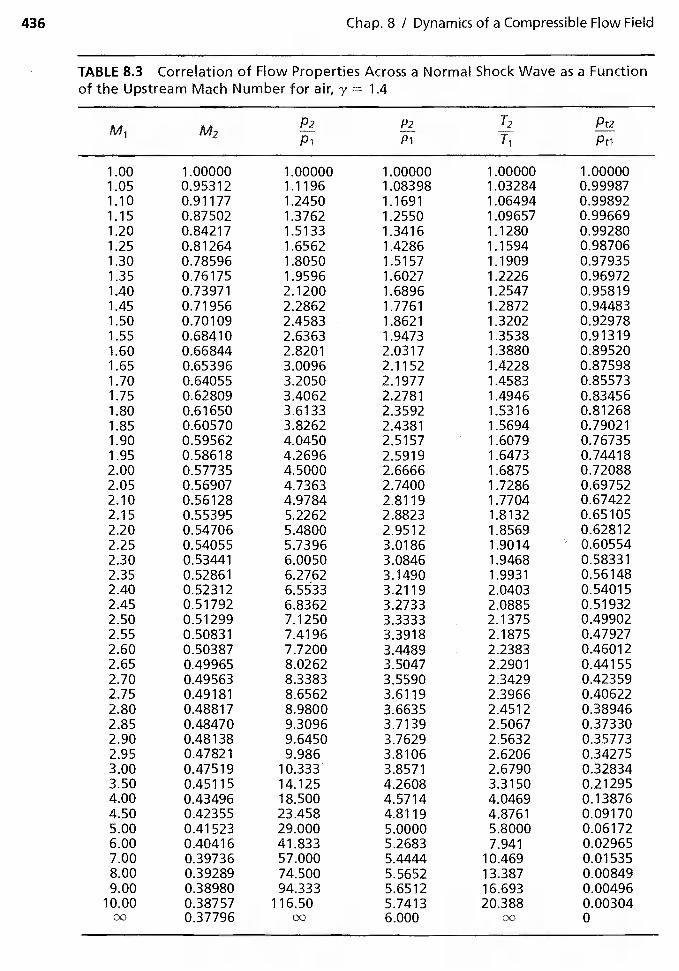
436 Chap. 8 / Dynamics of a Compressible Flow Field
TABLE 8.3 Correlation of Flow Properties Across a Normal Shock Wave as a Functionof the Upstream Mach Number for air, 'y = 1.4
P2M1 PA2
P2 T2 pQ
1.00 1.00000 1.00000 1.00000 1.00000 1.000001.05 0.95312 1.1196 1.08398 1.03284 0.999871.10 0.91177 1.2450 1.1691 1.06494 0.998921.15 0.87502 1.3762 1.2550 1.09657 0.996691.20 0.84217 1.5133 1.3416 1.1280 0.992801.25 0.81264 1.6562 1.4286 1.1594 0.987061.30 0.78596 1.8050 1.5157 1.1909 0.979351.35 0.76175 1.9596 1.6027 1,2226 0.969721.40 0.73971 2.1200 1.6896 1.2547 0.958191.45 0,71956 2.2862 1.7761 1.2872 0.944831.50 0.70109 2.4583 1.8621 1.3202 0.929781.55 0.68410 2.6363 1.9473 1.3538 0.913191.60 0.66844 2.8201 2.0317 1.3880 0.895201.65 0.65396 3.0096 2.1152 1.4228 0.875981.70 0.64055 3.2050 2.1977 1.4583 0.855731.75 0.62809 3.4062 2.2781 1.4946 0.834561.80 0.61650 3.6133 2.3592 1.5316 0.812681.85 0.60570 3.8262 2.4381 1.5694 0.790211.90 0.59562 4.0450 2.5157 1.6079 0.767351.95 0.58618 4.2696 2.5919 1.6473 0.744182.00 0.57735 4.5000 2.6666 1.6875 0.720882.05 0.56907 4.7363 2.7400 1.7286 0.697522.10 0.56128 4.9784 2.8119 1.7704 0.674222.15 0.55395 5.2262 2.8823 1.8132 0.651052.20 0.54706 5.4800 2.9512 1.8569 0.628122.25 0.54055 5.7396 3.0186 1.9014 0.605542.30 0.53441 6.0050 3.0846 1.9468 0.583312.35 0,52861 6.2762 3.1490 1.9931 0.561482.40 0.52312 6.5533 3,2119 2.0403 0,540152.45 0.51792 6.8362 3.2733 2.0885 0.519322.50 0.51299 7.1250 3.3333 2.1375 0.499022.55 0.50831 7.4196 3.3918 2.1875 0.479272.60 0.50387 7.7200 3.4489 2.2383 0.460122.65 0.49965 8.0262 3.5047 2.2901 0.441 552.70 0.49563 8.3383 3.5590 2.3429 0.423592.75 0.49181 8.6562 3.6119 2.3966 0.406222.80 0.48817 8.9800 3.6635 2.4512 0.389462.85 0.48470 9.3096 3.71 39 2.5067 0.373302.90 0.481 38 9.6450 3.7629 2.5632 0.357732.95 0.47821 9.986 3.8106 2.6206 0.342753.00 0.47519 10.333 3.8571 2.6790 0.328343.50 0.45115 14.125 4.2608 3.3150 0.212954.00 0.43496 18.500 4.5714 4.0469 0.138764.50 0.42355 23.458 4.8119 4.8761 0.091705.00 0.41523 29.000 5.0000 5.8000 0.061726.00 0.40416 41.833 5.2683 7.941 0.029657.00 0.39736 57.000 5.4444 10.469 0.015358.00 0.39289 74.500 5.5652 13.387 0.008499.00 0.38980 94.333 5.6512 16.693 0.00496
10.00 0.38757 116.50 5.7413 20.388 0.00304Do 0.37796 00 6.000 00 0
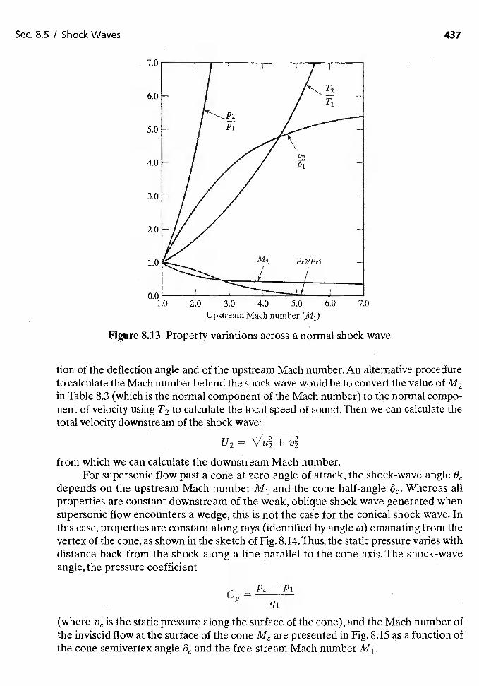
Sec. 8.5 / Shock Waves 437
Figure 8.13 Property variations across a normal shock wave.
tion of the deflection angle and of the upstream Mach number. An alternative procedureto calculate the Mach number behind the shock wave would be to convert the value of M2in Table 8.3 (which is the normal component of the Mach number) to the normal compo-nent of velocity using T2 to calculate the local speed of sound. Then we can calculate thetotal velocity downstream of the shock wave:
U2 = +
from which we can calculate the downstream Mach number.For supersonic flow past a cone at zero angle of attack, the shock-wave angle
depends on the upstream Mach number M1 and the cone half-angle Whereas allproperties are constant downstream of the weak, oblique shock wave generated whensupersonic flow encounters a wedge, this is not the case for the conical shock wave. Inthis case, properties are constant along rays (identified by angle emanating from thevertex of the cone, as shown in the sketch of Fig. 8.14. Thus, the static pressure varies withdistance back from the shock along a line parallel to the cone axis. The shock-waveangle, the pressure coefficient
c — Pc — Pip
(where is the static pressure along the surface of the cone), and the Mach number ofthe inviscid flow at the surface of the cone are presented in Fig. 8.15 as a function ofthe cone semivertex angle and the free-stream Mach number M1.
1.0 2.0 3.0 4.0 5.0 6.0 7.0
Upstream Mach number (Mi)
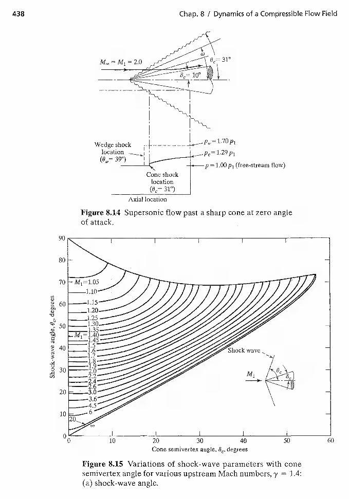
438
0
0C
rID
Chap. 8 / Dynamics of a Compressible Flow Field
= 1.00 Pi (free-stream flow)
Figure 8.14 Supersonic flow past a sharp cone at zero angleof attack.
Figure 8.15 Variations of shock-wave parameters with conesemivertex angle for various upstream Mach numbers, y 1.4:(a) shock-wave angle.
= = 2.0
39°)
Axial location
00 10 20 30 40
Cone semivertex angle, degrees
50
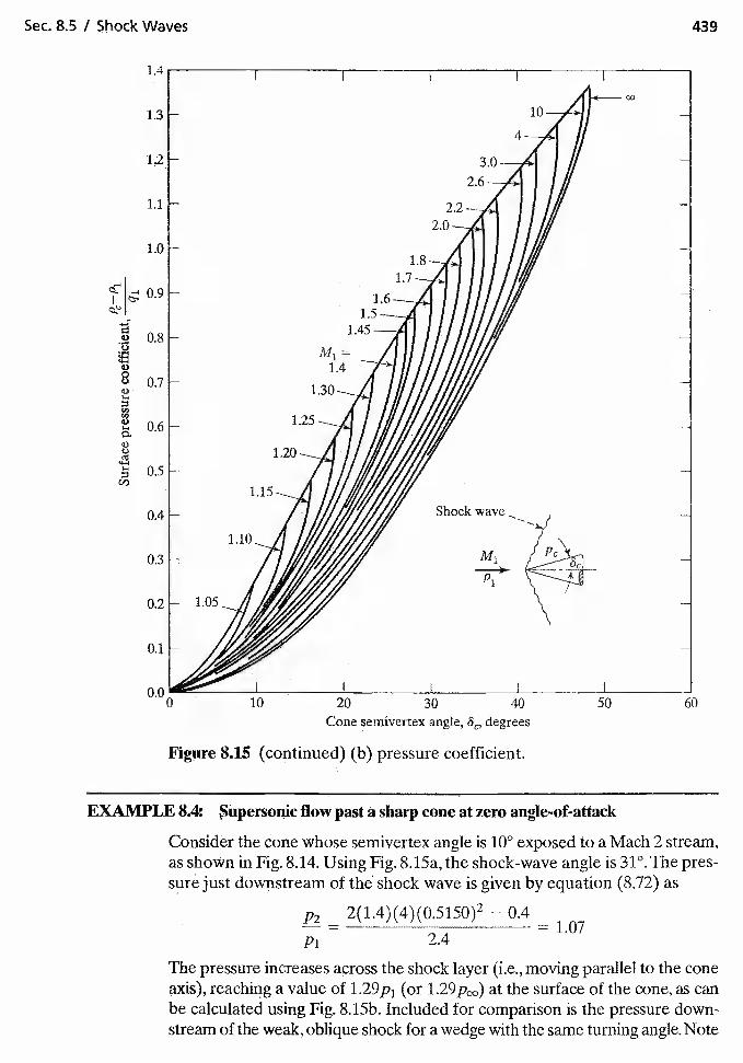
Sec. 8.5 I Shock Waves
U
0U
3,.
(I)
3-.
Figure 8.15 (continued) (b) pressure coefficient.
439
8.4: Supersonic flow past a sharp cone at zero angle-of-attack
consider the cone whose semivertex angle is 10° exposed to a Mach 2 stream,as shown in Fig. 8.14. Using Fig. 8.15a, the shock-wave angle is 31°. The pres-sure just downstream of the shock wave is given by equation (8.72) as
2(1.4)(4)(0,5150)2 — 0.4_ 1.07
P1
The pressure increases across the shock layer (i.e., moving parallel to the coneaxis), reaching a value of 1 .29Pi (or at the surface of the cone, as canbe calculated using Fig. 8.15b. Included for comparison is the pressure down-stream of the weak, oblique shock for a wedge with the same turning angle. Note
20 30 40
Cone semivertex angle, degrees
2.4
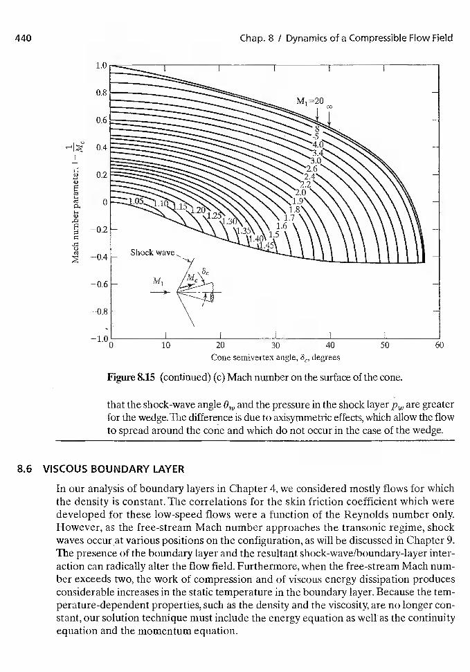
440 Chap. 8 / Dynamics of a Compressible Flow Field
a)
a)
I-.
a)
C-.
C)Cl
Figure 8.15 (continued) (c) Mach number on the surface of the cone.
that the shock-wave angle and the pressure in the shock layer Pw are greaterfor the wedge. The difference is due to axisymmetric effects, which allow the flowto spread around the cone and which do not occur in the case of the wedge.
8.6 VISCOUS BOUNDARY LAYER
In our analysis of boundary layers in Chapter 4, we considered mostly flows for whichthe density is constant. The correlations for the skin friction coefficient which weredeveloped for these low-speed flows were a function of the Reynolds number only.However, as the free-stream Mach number approaches the transonic regime, shockwaves occur at various positions on the configuration, as will be discussed in Chapter 9.The presence of the boundary layer and the resultant shock-wave/boundary-layer inter-action can radically alter the flow field. Furthermore, when the free-stream Mach num-ber exceeds two, the work of compression and of viscous energy dissipation producesconsiderable increases in the static temperature in the boundary layer. Because the tem-perature-dependent properties, such as the density and the viscosity, are no longer con-stant, our solution technique must include the energy equation as well as the continuityequation and the momentum equation.
30 40
Cone semivertex angle, degrees
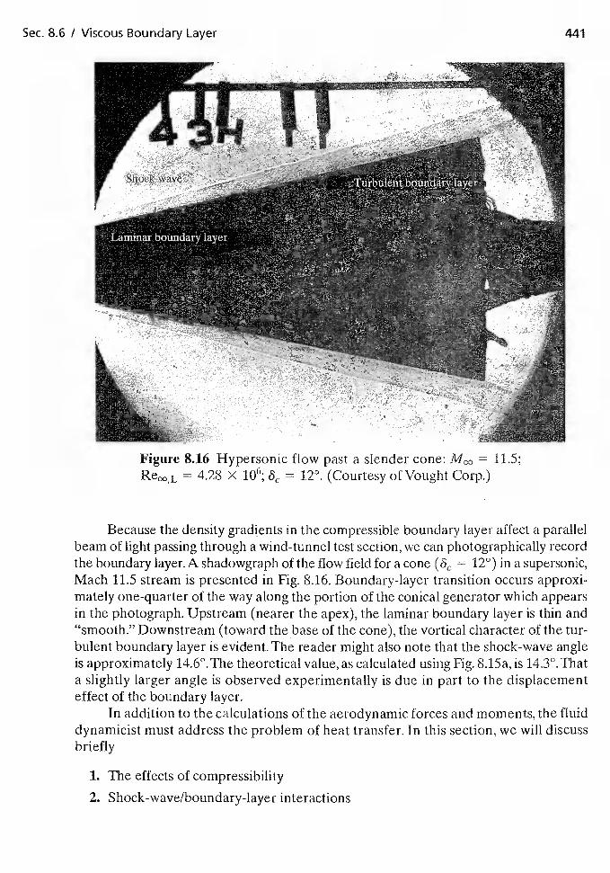
Sec. 8.6 / Viscous Boundary Layer 441
Because the density gradients in the compressible boundary layer affect a parallelbeam of light passing through a wind-tunnel test section, we can photographically recordthe boundary layer.A shadowgraph of the flow field for a cone = 12°) in a supersonic,Mach 11.5 stream is presented in Fig. 8.16. Boundary-layer transition occurs approxi-mately one-quarter of the way along the portion of the conical generator which appearsin the photograph. Upstream (nearer the apex), the laminar boundary layer is thin and"smooth." Downstream (toward the base of the cone), the vortical character of the tur-bulent boundary layer is evident. The reader might also note that the shock-wave angleis approximately 14.6°. The theoretical value, as calculated using Fig. 8.15a, is 14.3°.Thata slightly larger angle is observed experimentally is due in part to the displacementeffect of the boundary layer.
In addition to the calculations of the aerodynamic forces and moments, the fluiddynamicist must address the problem of heat transfer. In this section, we will discussbriefly
1. The effects of compressibility
2. Shock-wave/boundary-layer interactions
Figure 8.16 Hypersonic flow past a slender cone: = 11.5;
ReOO,L = 4.28 X 10⁶; = 12°. (Courtesy of Vought Corp.)
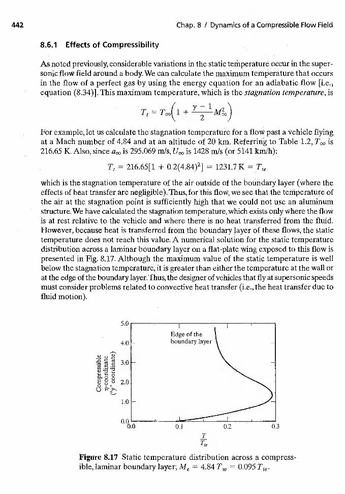
Chap. 8 / Dynamics of a Compressible Flow Field
8.6.1 Effects of Compressibility
As noted previously, considerable varintions in the static temperature occur in the super-sonic flow field around a body. We can calculate the maximum temperature that occursin the flow of a perfect gas by using the energy equation for an adiabatic flowequation (8.34)]. This maximum teniperature, which is the stagnation temperature, is
For example, let us calculate the stagnation temperature for a flow past a vehicle flyingat a Mach number of 4.84 and at an altitude of 20 km. Referring to Table 1.2, is216.65 K. Also, since is 95.069 m/s, is 1428 m/s (or 5141 km/h):
216.65[1 + 0.2(4.84)21 = 1231.7 K = Tte
which is the stagnation temperature of the air outside of the boundary layer (where theeffects of heat transfer are negligible).Thus, for this flow, we see that the temperature ofthe air at the stagnation point is sufficiently high that we could not use an aluminumstructure. We have calculated the stagnation temperature, which exists only where the flowis at rest relative to the vehicle and where there is no heat transferred from the fluid.However, because heat is transferred from the boundary layer of these flows, the statictemperature does not reach this value. A numerical solution for the static temperaturedistribution across a laminar boundary layer on a flat-plate wing exposed to this flow ispresented in Fig. 8.17. Although the maximum value of the static temperature is wellbelow the stagnation temperature, it is greater than either the temperature at the wall orat the edge of the boundary layer. Thus, the designer of vehicles that fly at supersonic speedsmust consider problems related to convective heat transfer (i.e., the heat transfer due tofluid motion).
0.3
Figure 8.17 Static temperature distribution across a compress-ible, laminar boundary layer; Me = 4.84 = 0.095 Tte.
TTte
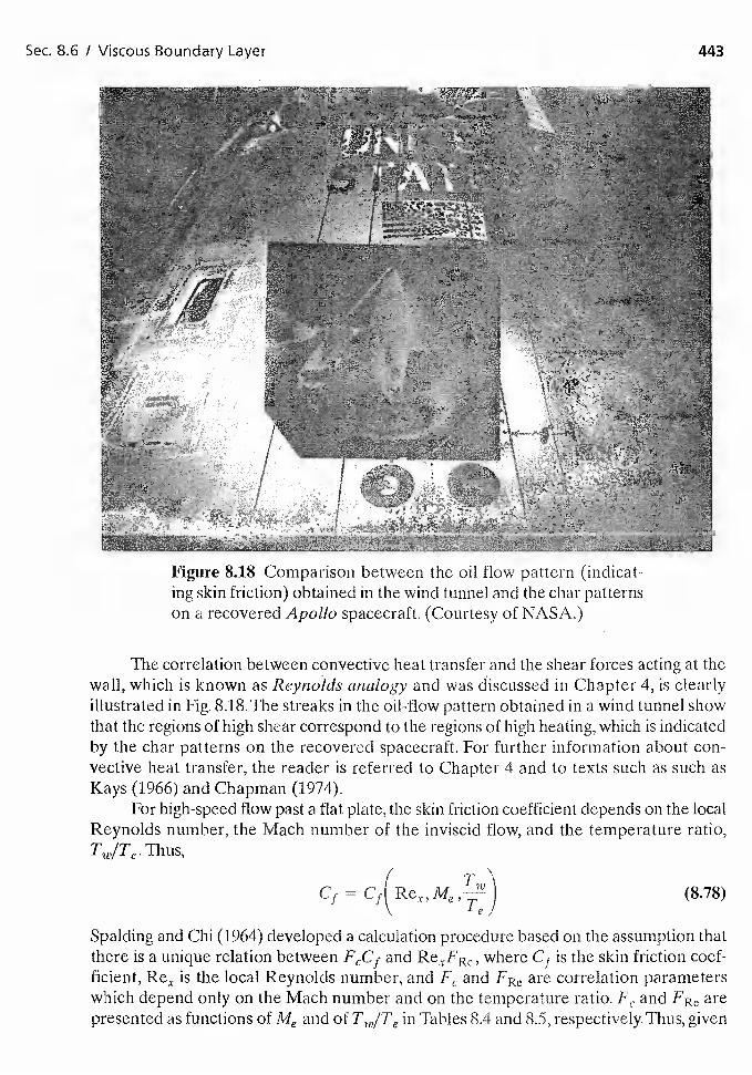
Sec. 8.6 / Viscous Boundary Layer 443
The correlation between convective heat transfer and the shear forces acting at thewall, which is known as Reynolds analogy and was discussed in Chapter 4, is clearlyillustrated in Fig. 8.18. The streaks in the oil-flow pattern obtained in a wind tunnel showthat the regions of high shear correspond to the regions of high heating, which is indicatedby the char patterns on the recovered spacecraft. For further information about con-vective heat transfer, the reader is referred to Chapter 4 and to texts such as such asKays (1966) and Chapman (1974).
For high-speed flow past a flat plate, the skin friction coefficient depends on the localReynolds number, the Mach number of the inviscid flow, and the temperature ratio,
Thus,
Cf = (8.78)
Spalding and Chi (1964) developed a calculation procedure based on the assumption thatthere is a unique relation between and RevFRe, where is the skin friction coef-ficient, is the local Reynolds number, and and are correlation parameterswhich depend only on the Mach number and on the temperature ratio. and FRe arepresented as functions of Me and of in Tables 8.4 and 8.5, respectively. Thus, given
Figure 8.18 Comparison between the oil flow pattern (indicat-ing skin friction) obtained in the wind tunnel and the char patternson a recovered Apollo spacecraft. (Courtesy of NASA.)
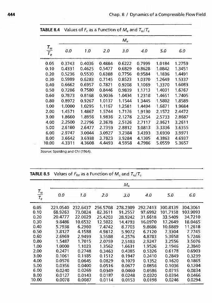
444 Chap. 8 / Dynamics of a Compressible Flow Field
TABLE 8.4 Values of as a Function of Me and Tw/Te
Me
Tie
'e0.0 1.0 2.0 3.0 4.0 5.0 6.0
0.050.100.200.300.400.500.600.801.002.003.004.005.006.008.00
10.00
0.37430.43310.52360.59890.66620.72860.78730.89721.00001.45711.86602.25002.61802.97473.66424.3311
0.40360.46250.55300.62830.69570.75800.81680.92671.02951.48671.89562.27962.64773.00443.69384.3608
0.48840.54770.63880.71450.78210.84460.90361.01371.11671.57441.98362.36782.73593.09273.78234.4493
0.62220.68290.77560.85230.92080.98391.04341.15441.25811.71762.12782.51262.88123.23843.92844.5958
0.79990.86280.95841.03701.10691.17131.23181.34451.44941.91302.32542.71173.08133.43934.13054.7986
1.01841.08421.18361.26491.33701.40311.46511.58021.68712.15722.57332.96213.33363.69304.38635.0559
1.27591.34511.44911.53371.60831.67671.74051.85891.96842.44722.86873.26113.63553.99714.69375.3657
Source: Spalding and Chi (1964).
TABLE 8.5 Values o f FRe as a Function of Me and T?v/Te
Me
1e0,0 1.0 2.0 3.0 4.0 5.0 6.0
0.05 221.0540 232.6437 256.5708 278.2309 292.7413 300.8139 304.30610.10 68.9263 73.0824 82.3611 91.2557 97.6992 101.7158 103.90930.20 20.4777 22.0029 25.4203 28.9242 31.6618 33.5409 34.72100.30 9.8486 10.6532 12.5022 14.4793 16.0970 17.2649 18.04650.40 5.7938 6.2960 7.4742 8.7703 9.8686 10.6889 11.26180.50 3.8127 4.1588 4.9812 5.9072 6.7120 7.3304 7.77450.60 2.6969 2.9499 3.5588 4.2576 4.8783 5.3658 5.72460.80 1.5487 1.7015 2.0759 2.5183 2.9247 3.2556 3.50761.00 1.0000 1.1023 1.3562 1.6631 1.9526 2.1946 2.38402.00 0.2471 0.2748 0.3463 0.4385 0.5326 0.6178 0.69033.00 0.1061 0.1185 0.1512 0.1947 0.2410 0.2849 0.32394.00 0.0576 0.0645 0.0829 0.1079 0.1352 0.1620 0.18655.00 0.0356 0.0400 0.0516 0.0677 0.0856 0.1036 0.12046.00 0.0240 0.0269 0.0349 0.0460 0.0586 0.0715 0.08348.00 0.0127 0.0143 0.0187 0.0248 0.0320 0.0394 0.0466
10.00 0.0078 0.0087 0.0114 0.0153 0.0198 0.0246 0.0294
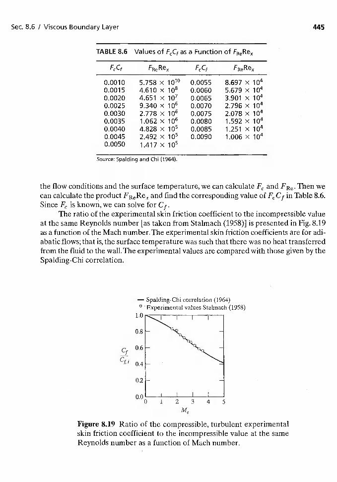
Sec.
8.6 Values of as a Function of FReReX
FRe FCCf FReRex
0.0010 5.758 x 10¹⁰ 0.0055 8.697 x0.0015 4.610 x 10⁸ 0.0060 5.679 x0.0020 4.651 x i07 0.0065 3.901 X0.0025 9.340 x 10⁶ 0.0070 2.796 x0.0030 2.778 X 10⁶ 0.0075 2.078 x i040.0035 1.062 x 10⁶ 0.0080 1.592 x0.0040 4.828 X 0.0085 1.251 x0.0045 2.492 X 0.0090 1.006 X0.0050 1.417 x
the flow conditions and the surface temperature, we can calculate and FRe. Then wecan calculate the product FReRex and find the corresponding value of Cj in Table 8.6.Since is known, we can solve for Cf.
The ratio of the experimental skin friction coefficient to the incompressible valueat the same Reynolds number [as taken from Stalmach (1958)] is presented in Fig. 8.19as a function of the Mach number. The experimental skin friction coefficients are for adi-abatic flows; that is, the surface temperature was such that there was no heat transferredfrom the fluid to the wall.The experimental values are compared with those given by theSpalding-Chi correlation.
Figure 8.19 Ratio of the compressible, turbulent experimentalskin friction coefficient to the incompressible value at the sameReynolds number as a function of Mach number.
Source: Spalding and Chi (1964).
Cf
— Spalding-Chi correlation (1964)o values Stalmach (1958)
1.0
0.8
0.6
0.4
0.2
0.00 1 2 3 4 5
446 Chap. 8 I Dynamics of a Compressible Flow Field
EXAMPLE 85: Skin-friction coefficient for a supersonic, turbulentboundary layer
What is the skin-friction coefficient for a turbulent boundary layer on a flatplate, when Me = 2.5, 6.142 X 10⁶, and = 3.OTe?
Solution: For these calculations,
= 2.056 (see Table 8.4)
and
FRe = 0.1729 (see Table 8.5)
Thus,
ReXFRe = 1.062 x
Using Table 8.6, we obtain
= 0.0035
so that
Cf = 1.70 x
8.7 THE ROLE OF EXPERIMENTS FOR GENERATINGINFORMATION DEFINING THE FLOW FIELD
The tools that are available to the designers of aerospace vehicles include analyticalmethods, numerical methods, experimental programs using ground-testing facilities,and experimental programs using flight-test programs. Most of the material definingthe role of experiments in generating information defining the flow field has beentaken from an article written by Bertin and Cummings for the 2006 Annual Review ofFluid Mechanics.
8.7.1 Ground-Based Tests
Despite the remarkable advances in hardware and software for computational fluiddynamics (CFD) tools, when two critical "return-to-flight" (RTF) concerns were iden-tified in the aerothermodynamic environment of the Space Shuttle, very extensive wind-tunnel programs were conducted. One RTF concern dealt with the heating in the bipodregion during launch. The second concern was related to the aerodynamics forces andmoments during reentry. Wind-tunnel tests provided the majority of the aerothermalinformation required by the "return-to-flight" advisory teams. Computational fluiddynamics (CFD) solutions were used primarily to generate numerical values for use incomparisons with the experimental measurements.
Since there is no single ground-based facility capable of duplicating the high-speedflight environment, different facilities are used to address various aspects of the design
8.7 / The Role of Experiments for Generating Information Defining the Flow Field 447
problems associated with supersonic flight. Most of the measurements that are usedduring the design process to.define the aerothermodynamic environment (i. e., the aero-dynamic forces and rhoments, the surface ptessure distribution, and the heat-transferdistribution) are obtained in the following:
1. Conventional wind-tunnels2. Shock-heated wind-tunnels3. Shock tubes4. Arc-heated test facilities5. Ballistic, free-flight ranges
The parameters that can be simulated in ground-based test facilities include:
1. Free-stream Mach number2. Free-stream Reynolds number (and its influence on the character of the bound-
ary layer)3. Free-stream velocity4. Pressure altitude5. Total enthalpy of the flow6. Density ratio across the shock wave7. Test gas8. Wall-to-total temperature ratio9. Thermochemistry of the fibw field
Note that some of the parameters are interrelated (e. g., the free-stream velocity, thetotal enthalpy of the flow, the free-stream Mach number, and the wall-to-total tem-perature ratio). The critical heating to the bipod region occurs in the Mach numberrange from 3.5 to 4.0—just prior to staging at approximately 30,480 m (100,000 ft).Because the total temperature for Mach 4 flow at 30,480 m (100,000 ft) is approxi-mately 950 K (1710°R), one can simultaneously simulate the free-stream velocity, thetotal enthalpy of the flow, the free-stream Mach number, and the free-streamReynolds number in conventional wind-tunnel facilities. Two facilities in which onecan match these four parameters are the Supersonic Aerothermal Tunnel C at theArnold Development Center (AEDC) [Anderson and Matthews (1993)]and the LENS II facility at the Calspan-University at Buffalo Research Center(CUBRC) [Holden, et al. (1995)].
Note also. that, during a specific rUn of a wind-tunnel test program, the model tem-perature usually starts out at room temperature. The temperature measurements that areused to determine the heat-transfer rates to the model usually are made early during thetest run. Thus, the temperature of model surface remains relatively cool during the data-recording portion of the run. On the other hand, the relatively long exposure to thehigh-temperature flight environment causes the surface of the vehicle to become veryhot. As a result, the wall-to-total-temperature ratio in ground-based tests is usually wellbelow the flight value. To match the flight value of the wall-to-total-temperature ratio,
448 Chap. 8 / Dynamics of a Compressible Flow Field
the total temperature of the tunnel flow is reduced below the flight value. Thus, even forthis relatively benign flow, one does not match the flight values of all of the flow-fieldparameters.
In addition to the nine flow-field related parameters that were identified earlierin this section, additional factors must be considered when developing a test plan. Theadditional factors include:
1. Model scale2. Test time3. Types of data available4. Flow quality (including uniformity, noise, cleanliness, and steadiness)
In a statement attributed to J. Leith Potter, Trimmer, et al. (1986) noted that "Aero-dynamic modeling is the art of partial simulation." Thus, the test engineer must decidewhich parameters are critical to accomplishing the objectives of the test program. Infact, during the development of a particular vehicle, the designers most likely willutilize many different facilities with the run schedule, the model, the instrumentation,and the test conditions for each program tailored to answer specific questions. As statedby Matthews, et a!. (1984), "A precisely defined test objective coupled with compre-hensive pretest planning are essential for a successful test program."
There are many reasons for conducting ground-based test programs. Some objec-tives include the following:
Objective 1. Obtain data to define the aerodynamic forces and momentsand/or the heat-transfer distributions for complete configurationswhose complex flow fields resist computational modeling.
Objective 2. Use partial configurations to obtain data defining local-flow phe-nomena, such as the inlet flow field for hypersonic air-breathingengines or the shock/boundary-layer interactions associated withdeflected control surfaces (a body flap).
Objective 3. Obtain detailed flow-field data to be used in developing numeri-cal models for use in a computational algorithm (code validation).
Objective 4, Obtain measurements of parameters, such as the heat transferand the drag, to be used in comparison with computed flow-fieldsolutions over a range of configuration geometries and of flowconditions (code calibration).
Objective 5. Obtain data that can be used to develop empirical correlationsfor phenomena that resist analytical and/or numerical modeling,such as boundary-layer transition and turbulence modeling.
Objective 6. Certify the performance of air-breathing engines.
Even today, extensive ground-based test-programs are conducted during thedesign process in order to define the aerothermodynamic environment for the entirevehicle. When the access to space study that was conducted by NASA in the early 1990srecommended the development of a fully reusable launch vehicle (RLV) [Bekey et al.
joined an industry-led technology-development effort for the X-33/RLV.
Sec. 8.7 / The Role of Experiments for Generating Information Defining the Flow Field 449
As part of the industry/government partnership, personnel and facilities at the LangleyResearch Center (NASA) were assigned the task of providing information regarding theaerodynamic forces and moments, the surface heating, and the criteria for boundary-layer transition to Lockheed Martin in support of X-33 development and design.
A special section in the September—October 2001 issue of the Journal of Spacecraftand Rockets presented five archival journal articles, documenting the results from thiscooperative effort. Two articles presented information relating to objective (1) "Obtaindata to define the aerodynamic forces and moments and/or the heat-transfer distribu-tions for complete configurations whose complex flow fields resist computational mod-eling." They are Horvath, et al. (2001) and Murphy, et a!. (2001). Two articles presentedinformation relating to objective (4) "Obtain measurements of parameters, such as theheat transfer and the drag, to be used in comparison with computed flow-field solutionsover, a range of configuration geometries and of flow conditions (code calibration)."They are Hollis, et al. (2001a) and Hollis, et al. (2001b). One article [Berry, et al. (2001a)}related to objective (5) "Obtain data that can be used to develop empirical correlationsfor phenomena that resist analytical and/or numerical modeling, such as boundary-layertransition and turbulence modeling."
"In 1996 NASA initiated the Hyper-X program as part of an initiative to maturethe technologies associated with hypersonic air-breathing propulsion." [Engelund(2001)]. "The primary goals of the Hyper-X program are to demonstrate and validate thetechnologies, the experimental techniques, and the computational methods and toolsrequired to design and develop hypersonic aircraft with airframe-integratçd, dual-modescramjet propulsion systems." Although hypersonic air-breathing propulsion systemshave been studied in the laboratory environment for over forty years, a complete air-frame-integrated vehicle configuration had never been flight tested. Again, personnel andfacilities at the Langley Research Center (NASA) were used to define the aerodynamicand surface heating environments, including information relating to the boundary-layertransition criteria, as part of the design, the development, the construction, and the flight-test program, for the X-43. .
A special section in the November—December 2001 issue of the Journal of Space-craft and Rockets presented seven archival journal articles summarizing the results fromthis program. Two articles presented information relating to objective (1) "Obtain datato define the aerodynamic forces and moments and/or the heat-transfer distributions forcomplete configurations whose complex flow fields resist computational modeling."They are Engelund, et al. (2001) and Holland, et a!. (2001). One article presented infor-mation relating to objective (4) "Obtain measurements of parameters, such as the heattransfer and the drag, to be used in comparison with computed flow-field solutions overa range of configuration geometries and of flow conditions (code calibration)." Thatwas by Cockrell, et a!. (2001). One article [Berry, et a!. (2001b)] related to objective(5) "Obtain data that can be used to develop empirical correlations for phenomena thatresist analytical and/or numerical modeling, such as boundary-layer transition and.tur-bulence modeling."
As described by Woods, et al. (2001), the Hyper-X Research Vehicle also called(HXRV or free flyer) required a booster to deliver the vehicle to the engine test points.The test conditions for the first flight included = 7 and 47,879 N/rn2 (1000psf) at an altitude of approximately 28,956 rn (95,000 ft). The Hyper-X Launch Vehicle
450 Chap. 8 / Dynamics of a Compressible Flow Field
(HXLV) stack was initially carried aloft under the wing of a B-52. The HXLV wasdropped, the Pegasus ignited, and the stack accelerated to the desired test Mach nuni-ber, When the stack reached the desired test conditions and attitude, a stage-separationsequence of events separated the free flyer from the booster. The free-flying researchvehicle then followed a preprogrammed trajectory. Although occurring in less than 500ms, stage separation was critical to reaching the engine test point and, hence, wascritical to mission success,
Buning, et al. (2001) reported that: "Even following the AEDC test, several aero-dynamic issues remained in fully understanding the dynamics of the stage separationmaneuver. This understanding was complicated by the unsteady nature of the event, thenumber of degrees of freedom associated with the booster, research vehicle, and controlsurfaces; and limits in the amount of wind-tunnel data available. These issues were inthree basic areas: unsteady effects, aerodynamic database extrapolation, and differencesbetween wind-tunnel and flight conditions." Viscous and inviscid computational fluiddynamics (CFD) techniques were used to quantify unsteady effects, to examine thecause and the extent of interference between the booster and the research vehicle, andto identify differences between the wind-tunnel and the flight environments.
8.7.2 Flight Tests
Flight tests are very expensive. Flight tests take a long time to plan and to execute suc-cessfully. FurthermOre, it is difficult to obtain quality data at well-defined test condi-tions. Flight tests will never replace ground-based tests or CFD in the design process.Nevertheless, flight tests are critical to our understanding of the hypersonic aerother-modynamic environment, since they provide data which cannot be obtained elsewhere.
Neumann (1988) suggests that there are a variety of reasons for conducting flighttests. Four reasons were suggested by Buck et al. (1963):
1. To demonstrate interactive technologies and to identify unanticipated problems.2. To form a catalyst (or a focus) for technology.3. To gain knowledge not only from the flights but also from the process of development.4. To demonstrate technology in flight so that it is credible for larger-scale applications.
Neumann added three reasons of his own:
5. To verify ground-test data and/or to understand the bridge between ground-testsimulations and actual flight.
6. To validate the overall performance of the system.7. To generate information not available on the ground.
Williamson (1992) noted: "Due to the large investment in flight testing, it is thendesirable to make as many measurements as possible during the flight to help verifypredictions or explain any modeling inaccuracies. The instrumentation should measureas directly as possible the things that have been predicted.This is often not possible andit is often necessary to infer predictions from related but not direct measurements."

Sec. 8.7 / The Role of Experiments for Generating Information Defining the Flow Field
Neumann (1989) stated: "Heat transfer is a quantity which cannot be directly measured:It is interpreted within the context of a thermal model rather than measured." Thus, onemust be able to develop a numerical model that describes the relation between the mea-sured temperature and the sensor's design, in order to obtain a reasonably accuratevalue of the experimentally-determined heat transfer. However, one also must developa numerical model depicting how the heat-transfer sensor responds from its location inthe vehicle. Serious problems can occur when the heat sensor is not properly integratedinto the flight structure such that minimal thermal distortion is produced.
Williamson (1992) notes that "Measurements fall into three groups. These includeatmospheric properties measurements, offboard vehicle related sensor measurements,and onboard vehicle related measurements telemetered to the ground or stored on tapeand retrieved post-flight."
There are two types of flight-test programs: (1) Research and Development (Rand D) programs and (2) flights of prototype or operational vehicles. R and D pro-grams are focused on technical issues which drive the design of the vehicle and itsflight operations. Iliff and Shafer (1992) noted that: "In the 1960's, several programssuccessfully generated aerothermodynamic flight data to improve the understandingand interpretationof theoretical and ground test results. The ASSET and PRIME pro-grams were flown in the early 1960's and provided aerothermodynamic flight data forablative and metallic thermal protection (TPS) concepts." Project Fire providedcalorimeter heating measurements on a large-scale blunt body entering the earth'satmosphere at an initial velocity 11.35 km/s (37.24 kft/s). As discussed by Cornette(1966), the forebody of the "Apollo-like" reentry capsule was constructed of threeberyllium calorimeter shields, which were alternated with phenolic-asbestos heatshields. This multiple-layer arrangement provided three distinct time periods whenmeasurements defining the aerothermodynamic environment could be obtained. TheFIRE program provided flight data that was used to understand radiative heat-trans-fer that become important for flight through the earth's atmosphere and when re-turning from lunar and from planetary missions [Ried, et al. (1972) and Sutton (1985)].
Flight-test data have been obtained on prototype vehicles, [e. g., the flights ofthe unmanned Apollo Command Modules (017 and 020) as discussed in Lee andGoodrich (1972)] and on operational vehicles [e. g., the Space Shuttle Orbiter, NASA(1995)].Throckmorton (1993) noted that the concept of using the Shuttle Orbiter asa flight research vehicle as an adjunct to its normal operational mission was a topicof discussion within the research community throughout the 1970s. Aerothermody-narnic parameters based on flight-test data obtained from thermocouples embeddedin the Space Shuttle Thermal Protection System (TPS) were used to expand the flightenvelope for the Orbiter. As noted by Hodge and Audley (1983), "Requirements forthe technique include an analytical model for the simulation of the heat transfer toa point on the TPS, flight test maneuvers which cause the thermocouples imbeddednear the surface of the TPS to respond sufficiently above the noise levels, and a para-meter estimation program to reduce flight thermocouple data. ... The data reductionprogram correlates heating with the variables such as angle of attack, sideslip, con-trol surface deflection, and Reynolds number. This technique could also be used forwind tunnel data reduction."
452 Chap. 8 / Dynamics of a Compressible Flow Field
The interactions between impinging shock waves and the bow shock wave can pro-duce locally severe heat-transfer rates. Edney (1968) identified six different shock/shockinteractions patterns. The positive deflection of the Orbiter body flap creates a shockwave which interacts with the boundary layer on the Orbiter. The adverse pressure gra-dient produced by the shock wave causes the boundary layer to thicken and (in manycases) to separate. The upstream extent of the interaction-produced perturbations de-pends on the size of the subsonic portion of the approach boundary layer and on thestrength of the shock wave produced by the turning of the flow. Thus, as noted by Bertin(1994), the parameters that influence the extent of an interaction are (1) whether the ap-proach boundary layer is laminar or turbulent, (2) the Mach number of the approachflow, (3) the Reynolds number of the approach flow, (4) the surface temperature, (5) thedeflection angle of the ramp, and (6) the chemical state of the gas. Bertin et a!. (1996) andFujii et al. (2001) investigated the perturbed flow fields due to deflected control surfacesusing the experimental values of the heat transfer measured during hypersonic flight.The HYFLEX vehicle [Fujii et al. (2001)] was a small-scale R and D vehicle whose lengthwas 4.40 m (14.44 ft).A two-stage launcher provided an initial altitude of 107 km (351 kft)at a velocity of 3.88 kmls (12.73 kft/s).
Despite the oft-mentioned problems with developing boundary-layer transitioncorrelations using flight-test measurements, there are numerous flight-test programswhere boundary-layer transition was a major focus of the data gathering efforts. West-on and Fitzkee (1963) noted that observed boundary-layer transition Reynolds num-bers on the Mercury capsule "agree well with Reynolds numbers obtained for waketransition behind spheres flown in a hypervelocity gun facility." Also flown in the1960's was the Reentry F vehicle which provided hypersonic boundary-layer transi-tion and is still used today. The Reentry F flight provided boundary-layer transitiondata at Mach numbers up to 20 and altitudes down to 24.38 km (80.00 kft) [Wrightand Zoby (1977)].
EXAMPLE 8.6: Wind-tunnel simulation of supersonic missile flow fields
Assume that you are given the task of determining the aerodynamic forcesand moments acting on a slender missile which flies at a Mach number of3.5 at an altitude of 27,432 m (90,000 ft). Aerodynamic coefficients for themissile, which is 20.0 cm (7.874 in) in diameter and 10 diameters long, arerequired for angles of attack from 0° to 55°. The decision is made to obtainexperimental values of the required coefficients in the Vouglit High-SpeedWind Tunnel (in Dallas, Texas). Upstream of the model shock system, theflow in the wind tunnel is isentropic and air, at these conditions, behaves asa perfect gas. Thus, the relations developed in this section can be used tocalculate the wind-tunnel test conditions.
Solution:
1. Flight conditions. Using the properties for a standard atmosphere (suchas were presented in Chapter 1), the relevant parameters for the flightcondition include
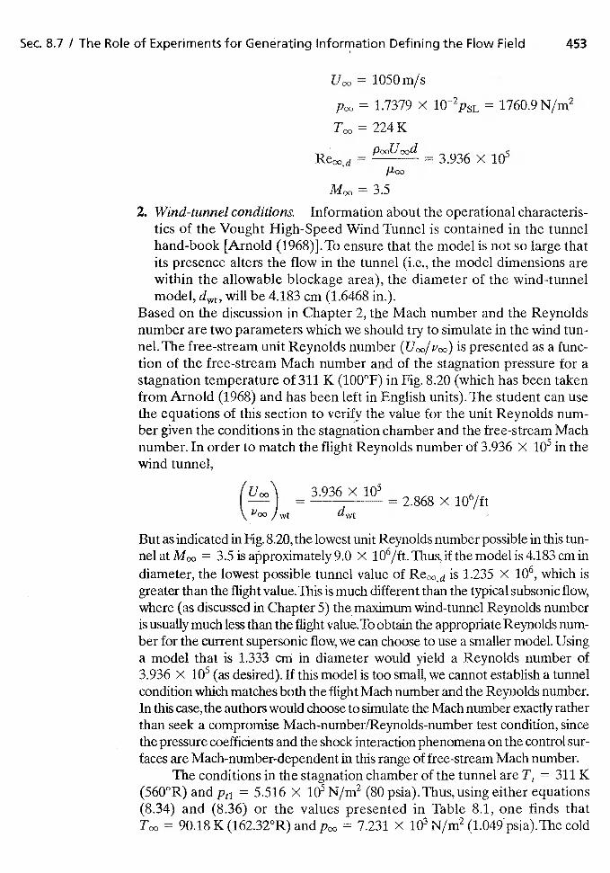
Sec. 8.7 / The Role of Experiments for Generating Information Defining the Flow Field 453
= 1050rn/s
= 1.7379 X IO2P5L = 1760.9 N/rn2
= 224K
d=
3.936 X i05
2. Wind-tunnel conditions. Information about the operational characteris-tics of the Vought High-Speed Wind Tunnel is contained in the tunnelhand-book [Arnold (1968)].To ensure that the model is not so large thatits presence alters the flow in the tunnel (i.e., the model dimensions arewithin the allowable blockage area), the diameter of the wind-tunnelmodel, will be 4.183 cm (1.6468 in.).
Based on the discussion in Chapter 2, the Mach number and the Reynoldsnumber are two parameters which we should try to simulate in the wind tun-nel. The free-stream unit Reynolds number is presented as a func-tion of the free-stream Mach number and of the stagnation pressure for astagnation temperature of 311 K (100°F) in Fig. 8.20 (which has been takenfrom Arnold (1968) and has been left in English units).The student can usethe equations of this section to verify the value for the unit Reynolds num-ber given the conditions in the stagnation chamber and the free-stream Machnumber. In order to match the flight Reynolds number of 3.936 X i05 in thewind tunnel,
= 3.936 X 102.868 X 106/ft
Jwt
But as indicated in Fig. 8.20, the lowest unit Reynolds number possible in this tun-nel at = 3.5 is approximately 9.0 x 10⁶/ft. Thus, if the model is 4.183 cm indiameter, the lowest possible tunnel value of is 1.235 X 10⁶, which isgreater than the flight value. This is much different than the typical subsonic flow,where (as discussed in Chapter 5) the maximum wind-tunnel Reynolds numberis usually much less than the flight value. To obtain the appropriate Reynolds num-ber for the current supersonic we can choose to use a smaller model. Usinga model that is 1.333 cm in diameter would yield a Reynolds number of3.936 x i05 (as desired). If this model is too small, we cannot establish a tunnelcondition which matches both the flight Mach number and the Reynolds number.In this case, the authors would choose to simulate the Mach number exactly ratherthan seek a compromise Mach-number[Reynolds-number test condition, sincethe pressure coefficients and the shock interaction phenomena on the control sur-faces are Mach-number-dependent in this range of free-stream Mach number.
The conditions in the stagnation chamber of the tunnel are 311 K(560°R) and Pti = 5.516 X N/rn2 (80 psia).Thus, using either equations(8.34) and (8.36) or the values presented in Table 8.1, one finds that
= 90.18 K (162.32°R) and = 7.231 x N/rn2 (1.049 psia).The cold
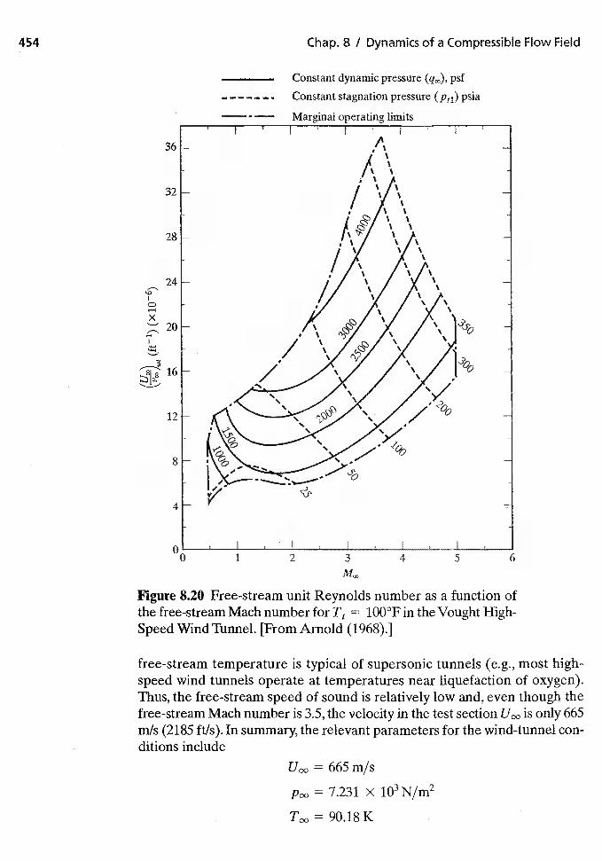
3
Figure 8.20 Free-stream unit Reynolds number as a function ofthe free-stream Mach number for — 100°F in the Vought High-Speed Wind Tunnel. [From Arnold (1968).}
free-stream temperature is typical of supersonic tunnels (e.g., most high-speed wind tunnels operate at temperatures near liquefaction of oxygen).Thus, the free-stream speed of sound is relatively low and, even though thefree-stream Mach number is 3.5, the velocity in the test section is only 665mIs (2185 ftls). In summary, the relevant parameters for the wind-tunnel con-ditions include
= 665 rn/s
7.231 X N/rn2
454 Chap. 8 / Dynamics of a Compressible Flow Field
Constant dynamic pressure (q.,), psf
- Constant stagnation pressure (Pu) psia
—. — Marginal operating limits
36
32 -
28 -
Ait
24 -
20 -
'a
x
16 -
12 -
8—
4
00 1 2 4 5 6
Sec. 8.9 / Shock-Wave/Boundary-Layer Interactions 455
= 3.936 X if d 1.333 cm or 1.235 X if d 4.183 cm
Moc,3.5Because of the significant differences in the dimensional values of the flowparameters (such as and we must again nondimensionalizethe parameters so that correlations of wind-tunnel measurements can be re-lated to the theoretical solutions or to the design flight conditions.
8.8 COMMENTS ABOUT THE SCALING/CORRECTIONPROCESS(ES) FOR RELATIVELY CLEAN CRUISECONFIGURATIONS
In an article for the Annual Review of Fluid Mechanics, Bushnell (2006) noted that "asurvey of 12 commercial transport aircraft, constructed by three major American man-ufacturers over a 20-year period showed that you are just as likely to estimate too higha drag as too low a drag. Six of the twelve (scaling) 'predictions' were low, four predic-tions were high, and two were right on. The drag predictions were as much as 22% lowand 10% high." Citing the work of other researchers, Bushnell (2006) noted that simi-lar values/discrepancies were obtained for airbreathing missiles. "As the experience fromthe various appliOations discussed herein indicates, 'surprise' occurs far too often and flowcomplexity can seriously degrade the 'scaled predictions'. Typical correction levelsinclude 6% wall interference, —5% Reynolds number, +2% roughness, and —4% stingand aeroelastic distortion effects. Total correction(s) from just these issues/concerns/ef-fects are the order of + 12%. On the other hand, the Viking aeroshell drag observedduring Martian entry agreed within some 2% of the scaled ground results, admittedlyfor a very bluff body with a fairly well characterized flow field."
8.9 SHOCK-WAVE/BOuNDARY-LAYER INTERAcTIONS
Severe problems of locally high heating or premature boundary-layer separation mayresult due to viscous/inviscid interactions which occur during flight at supersonic Machnumbers. The shock wave generated by a deflected flap will interact with the upstreamboundary layer. The interaction will generally cause the upstream boundary layer toseparate with locally high heating rates occurring when the flow reattaches. The extentof the separation, which can cause a loss of control effectiveness, depends on the char-acter of the upstream boundary-layer. Other viscous interaction problems can occurwhen the shock waves generated by the forebody and other external components im-pinge on downstream surfaces of the vehicle. Again, locally severe heating rates orboundary-layer separation may occur.
The basic features of the interaction between a shock wave and a laminar boundarylayer for a two-dimensional flow are shown in Fig. 8.21a. The pressure rise induced by theshock wave is propagated upstream through the subsonic portion of the boundary layer.Recall that pressure disturbances can affect the upstream flow only if the flow is subsonic.As a result, the boundary-layer thickness increases and the momentum decreases. Thethickening boundary layer deflects the external stream and creates a series of compression
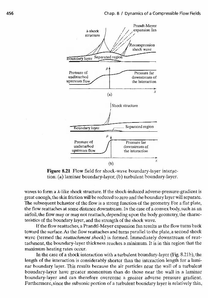
456 Chap. 8 I Dynamics of a Compressible Flow Fields
Prandt-MeyerA-shock fan
//,?/' ecompressionshock wave
oundary layer Separated region
p
__________________
Pressure of Pressure farundisturbed downstream of
upstream flow the interaction
(a)
Figure 821 Flow field for shock-wave boundary-layer interac-tion: (a) laminar boundary-layer; (b) turbulent boundary-layer.
waves to form a A-like shock structure. If the shock-induced adverse-pressure-gradient isgreat enough, the skin friction will be reduced to zero and the boundary layer will separate.The subsequent behavior of the flow is a strong function of the geometry. For a flat plate,the flow reattaches at some distance downstream. In the case of a convex body, such as anairfoil, the flow may or may not reattach, depending upon the body geometry, the charac-teristics of the boundary layer, and the strength of the shock wave.
If the flow reattaches, a Prandtl-Meyer expansion fan results as the flow turns backtoward the surface. As the flow reattaches and turns parallel to the plate, a second shockwave (termed the reattachment shock) is formed. Immediately downstream of reat-tachment, the boundary-layer thickness reaches a minimum. It is in this region that themaximum heating rates occur.
In the case of a shock interaction with a turbulent boundary-layer (Fig. 8.21b), thelength of the interaction is considerably shorter than the interaction length for a lami-nar boundary layer. This results because the air particles near the wall of a turbulentboundary-layer have greater momentum than do those near the wall in a laminarboundary-layer and can therefore overcome a greater adverse pressure gradient.Furthermore, since the subsonic portion of a turbulent boundary layer is relatively thin,
Shock structure
p4Pressure ofundisturbed
upstream flow
Pressure fardownstream ofthe interaction
(b)x
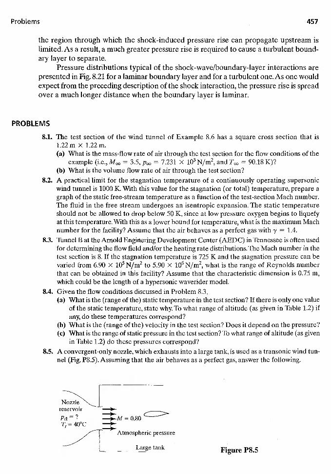
Problems 457
the region through which the shock-induced pressure rise can propagate upstream islimited. As a result, a much greater pressure rise is required to cause a turbulent bound-ary layer to separate.
Pressure distributions typical of the shock-wave/boundary-layer interactions arepresented in Fig. 8.21 for a laminar boundary layer and for a turbulent one. As one wouldexpect from the preceding description of the shock interaction, the pressure rise is spreadover a much longer distance when the boundary layer is laminar.
PROBLEMS
8.1. The test section of the wind tunnel of Example 8.6 has a square cross section that is1.22m X 1.22m.(a) What is the mass-flow rate of air through the test section for the flow conditions of the
example (i.e., = 3.5, = 7.231 x N/m2, and = 90.18 K)?(b) What is the volume flow rate of air through the test section?
8.2. A practical limit for the stagnation temperature of a continuously operating supersonicwind tunnel is .1000 K. With this value for the stagnation (or total) temperature, prepare agraph of the static free-stream temperature as a function of the test-section Mach number.The fluid in the free stream undergoes an isentropic expansion. The static temperatureshould not be allowed to drop below 50 K, since at low pressure oxygen begins to liquefyat this temperature. With this as a lower bound for temperature, what is the maximum Machnumber for the facility? Assume that the air behaves as a perfect gas with y = 1.4.
83. Tunnel B at the Arnold Enginering Development Center (AEDC) in Tennessee is often usedfor determining the flow field and/or the heating rate distributions. The Mach number in thetest section is 8. If the stagnation temperature is 725 K and the stagnation pressure can bevaried from 6.90 x i05 N/rn2 to 5.90 x 10⁶ N/m2, what is the range of Reynolds numberthat can be obtained in this facility? Assume that the characteristic dimension is 0.75 m,which could be the length of a hypersonic waverider model.
8.4. Given the flow conditions discussed in Problem 8.3,(a) What is the (range of the) static temperature in the test section? If there is only one value
of the static temperature, state why. To what range of altitude (as given in Table 1,2) ifany, do these temperatures correspond?
(b) What is the (range of the) velocity in the test section? Does it depend on the pressure?(c) What is the range of static pressure in the test section? To what range of altitude (as given
in Table 1.2) do these pressures correspond?8.5. A convergent-only nozzle, which exhausts into a large tank, is used as a transonic wind tun-
nel (Fig. P8.5). Assuming that the air behaves as a perfect gas, answer the following.
reservoir —3—
T,=40°CAtmospheric pressure
Large tank Figure P8.5
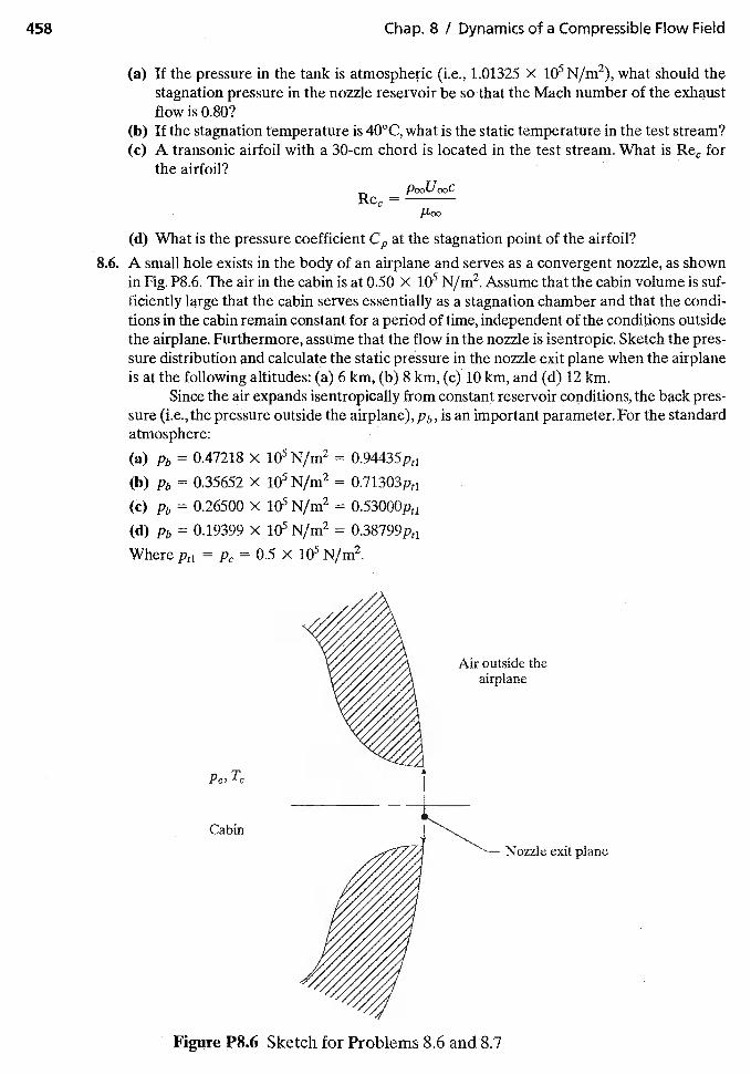
458 Chap. 8 / Dynamics of a Compressible Flow Field
(a) If the pressure in the tank is atmospheric (i.e., 1.01325 X N/rn2), what should thestagnation pressure in the nozzle reservoir be so that the Mach number of the exhaustflow is 0.80?
(b) lithe stagnation temperature is 40°C, what is the static temperature in the test stream?(c) A transonic airfoil with a 30-cm chord is located in the test stream. What is for
the airfoil?
/-too
(d) What is the pressure coefficient at the stagnation point of the airfoil?
8.6. A small hole exists in the body of an airplane and serves as a convergent nozzle, as shownin Fig. P8.6. The air in the cabin is at 0.50 X i05 N/rn2. Assume that the cabin volume is suf-ficiently large that the cabin serves essentially as a stagnation chamber and that the condi-tions in the cabin remain constant for a period of time, independent of the conditions outsidethe airplane. Furthennore, assume that the flow in the nozzle is isentropic. Sketch the pres-sure distribution and calculate the static pressure in the nozzle exit plane when the airplaneis at the following altitudes: (a) 6 km, (b) 8 km, (c) 10 km, and (d) 12 km.
Since the air expands isentropically from constant reservoir conditions, the back pres.sure (i.e., the pressure outside the airplane),pb, is an important parameter. For the standardatmosphere:
Where Pu = Pc = 0.5 X i05 N/rn2.
p,, T,,
Cabin
Figure P86 Sketch for Problems 8.6 and 8.7
Nozzle exit plane
(a) Pb = 0.47218 x(b) Pb = 0.35652 x(c) Pb = 0.26500 x(d) Pb = 0.19399 x
N/rn2 =i05 N/rn2 =1O5 N/rn2 = °.53000Ptii05 N/rn2 =
Air outside theairplane
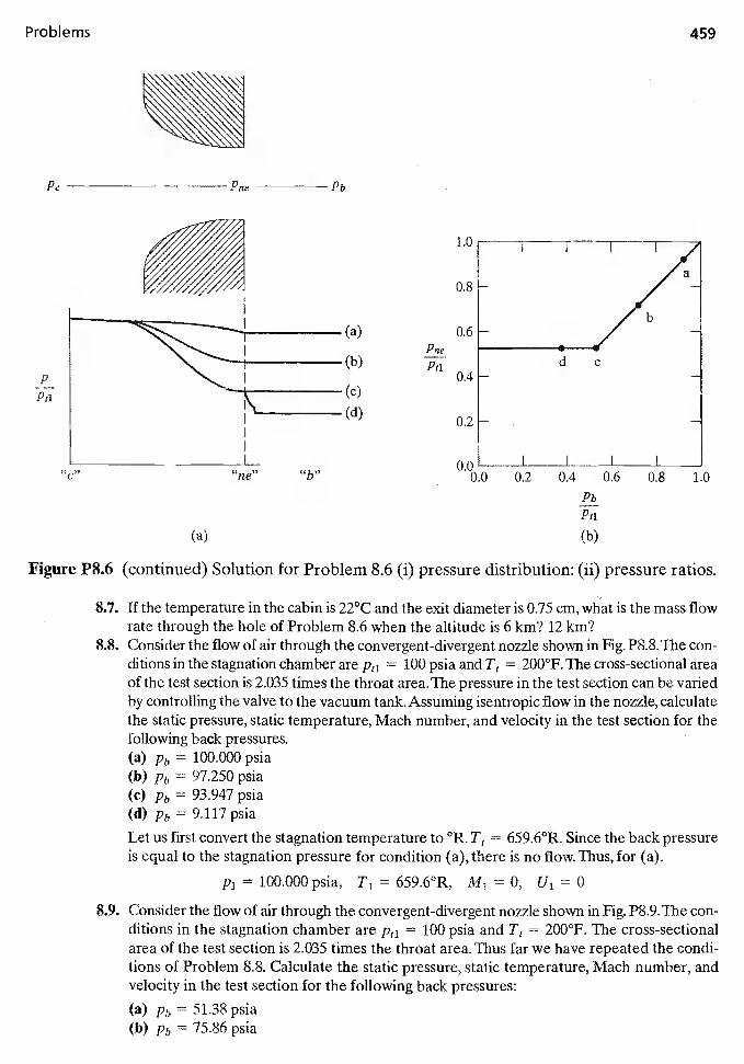
Problems 459
P
Pti
"C,,
(a)
Pt'
(b)
Figure P8.6 (continued) Solution for Problem 8.6 (i) pressure distribution: (ii) pressure ratios.
8.7. If the temperature in the cabin is 22°C and the exit diameter is 0.75 cm, what is the mass flowrate through the hole of Problem 8.6 when the altitude is 6 km? 12 km?
8.8. Consider the flow of air through the convergent-divergent nozzle shown in Fig. P8.8.The con-ditions in the stagnation chamber are Pti = 100 psia and T5 = 200°F. The cross-sectional areaof the test section is 2.035 times the throat area. The pressure in the test section can be variedby controlling the valve to the vacuum tank. Assuming isentropic flow in the nozzle, calculatethe static pressure, static temperature, Mach number, and velocity in the test section for thefollowing back pressures.(a) Pb = 100.000 psia(b) Pb = 97.250 psia(c) Pb = 93.947 psia(d) Pb 9.117 psia
Let us first convert the stagnation temperature to °R. T, = 659.6°R. Since the back pressureis equal to the stagnation pressure for condition (a), there is no flow. Thus, for (a).
Pi = 100.000 psia, T1 = 659.6°R, M1 = 0, U, = 0
8.9. Consider the flow of air through the convergent-divergent nozzle shown in Fig. P8.9. The con-ditions in the stagnation chamber are Psi = 100 psia and T5 = 200°F. The cross-sectionalarea of the test section is 2.035 times the throat area. Thus far we have repeated the condi-tions of Problem 8.8. Calculate the static pressure, static temperature, Mach number, andvelocity in the test section for the following back pressures:
(a) Pb = 51.38 psia(b) Pb = 75.86 psia
PC — Pne Pb
(a)
PbPti
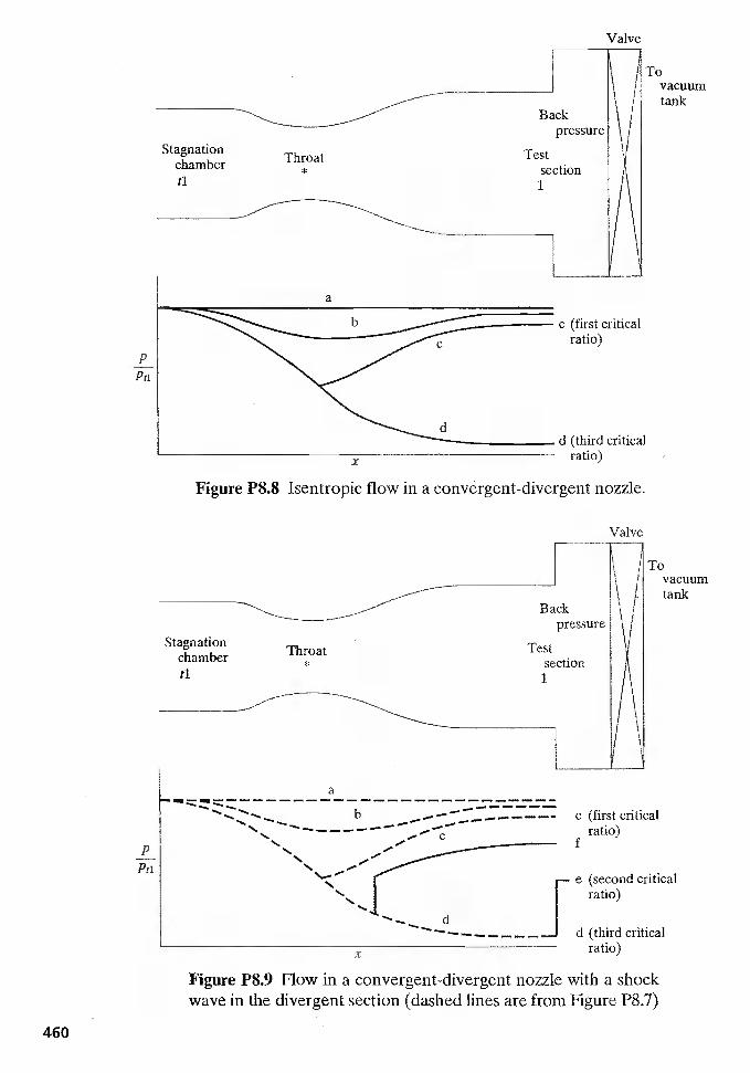
460
Figure P8.9 Flow in a convergent-divergent nozzle with a shockwave in the divergent section (dashed lines are from Figure P8.7)
Valve
Stagnationchamber Throat
tl
Back
Testsection
1
a
x
Tovacuumtank
c (first criticalratio)
d (third criticalratio)
Figure P8.8 Isentropic flow in a convergent-divergent nozzle.
Valve
Tovacuumtank
pressure I
Throat TestStagnationchamber section
a
b c (first critical— — — — — ratio)
fS..
e (second criticalS.
Jratio)S.
d (third criticalratio)
pPu
x
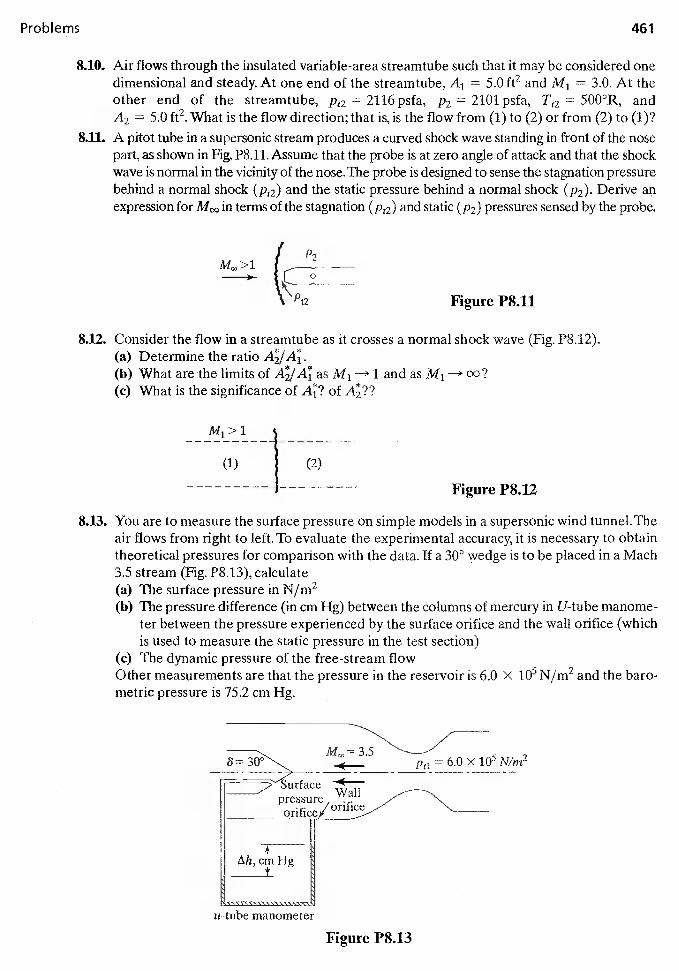
Problems 461
8.10. Air flows through the insulated variable-area streamtube such that it may be considered onedimensional and steady. At one end of the streamtube, A1 = 5.0 ft2 and M1 = 3.0. At theother end of the streamtube, Pt2 = 2116 psfa, P2 = 2101 psfa, = 500°R, andA2 5.0 ft2. What is the flow direction; that is, is the flow from (1) to (2) or from (2) to (1)?
8.11.. A pitot tube in a supersonic stream produces a curved shock wave standing in front of the nosepart, as shown in Fig. P8.11. Assume that the probe is at zero angle of attack and that the shockwave is normal in the vicinity of the nose.The probe is designed to sense the stagnation pressurebehind a normal shock (Pt2) and the static pressure behind a normal shock (P2). Derive anexpression for in terms of the stagnation (Pr2) and static (P2) pressures sensed by the probe.
I>1
{
Figure P8.11
8.12. Consider the flow in a streamtube as it crosses a normal shock wave (Fig. P8.12).(a) Determine the ratio AJ4.(b) What are the limits of A/At as M1 1 and as M1 oo?(c) What is the significance of 4? of
(2)
Figure P8.12
8.13. You are to measure the surface pressure on simple models in a supersonic wind tunnel. Theair flows from right to left. To evaluate the experimental accuracy, it is necessary to obtaintheoretical pressures for comparison with the data. If a 30° \vedge is to be placed in a Mach3.5 stream (Fig. P8.13), calculate(a) The surface pressure in N/rn2(b) The pressure difference (in cm Hg) between the columns of mercury in U-tube manome-
ter between the pressure experienced by the surface orifice and the wall orifice (whichis used to measure the static pressure in the test section)
(c) The dynamic pressure of the free-stream flowOther measurements are that the pressure in the reservoir is 6.0 X N/m2 and the baro-metric pressure is 75.2 cm Hg.
Figure P8.13
M1> 1
-
Wallpressure'orifice
u-tube manometer
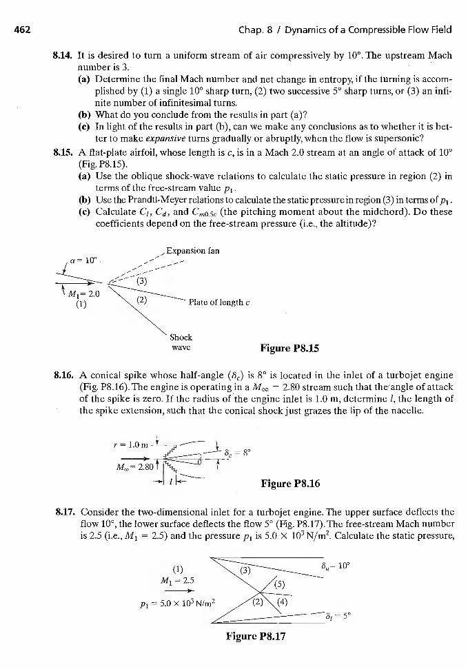
462 Chap. 8 / Dynamics of a Compressible Flow Field
8.14. It is desired to turn a uniform stream of air compressively by 100. The upstream Machnumber is 3.(a) Determine the final Mach number and net change in entropy, if the turning is accom-
plished by (1) a single 100 sharp turn, (2) two successive 50 sharp turns, or (3) an infi-nite number of infinitesimal turns.
(b) What do you conclude from the results in part (a)?(c) In light of the results in part (b), can we make any conclusions as to whether it is bet-
ter to make expansive turns gradually or abruptly, when the flow is supersonic?8.15. A flat-plate airfoil, whose length is c, is in a Mach 2.0 stream at an angle of attack of 10°
(Fig. P8.15).(a) Use the oblique shock-wave relations to calculate the static pressure in region (2) in
terms of the free-stream value(b) Use the Prandtl-Meyer relations to calculate the static pressure in region (3) in terms of(c) Calculate C1, Cd, and Cmø5c (the pitching moment about the midchord). Do these
coefficients depend on the free-stream pressure (i.e., the altitude)?
2.0(1)
— Expansion fan
Plate of length c
kwave Figure P8.15
8.16. A conical spike whose half-angle is 8° is located in the inlet of a turbojet engine(Fig. P8.16).The engine is operating in a = 2.80 stream such that theangle of attackof the spike is zero. If the radius of the engine inlet is 1.0 m, determine 1, the length ofthe spike extension, such that the conical shock just grazes the lip of the nacelle.
r=1.Om
____
S
Figure P8.16
8.17. Consider the two-dimensional inlet for a turbojet engine. The upper surface deflects theflow 100, the lower surface deflects the flow 5° (Fig. P8.17).The free-stream Mach numberis 2.5 (i.e., M1 = 2.5) and the pressure Pi is 5.0 )< i03 N/m2. Calculate the static pressure,
P1
Figure P8.17
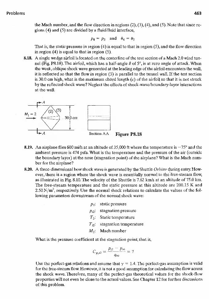
Problems 463
the Mach number, and the flow direction in regions (2), (3), (4), and (5). Note that since re-gions (4) and (5) are divided by a fluid/fluid interface,
and 0405That is, the static pressure in region (4) is equal to that in region (5), and the flow directionin region (4) is equal to that in region (5).
8.18. A single wedge airfoil is located on the centerline of the test section of a Mach 2.0 wind tun-nel (Fig. P8.18). The airfoil, which has a half-angle 5 of 50, is at zero angle of attack. Whenthe weak, oblique shock wave generated at the leading edge of the airfoil encounters the wall,it is reflected so that the flow in region (3) is parallel to the tunnel wall. If the test sectionis 30.0 cm high, what is the maximum chOrd length (c) of the airfoil so that it is not struckby the reflected shock wave? Neglect the effects of shock-wave/boundary-layer interactionsat the wall.
Section AA Figure P8.18
8.19. An airplane flies 600 mi/h at an altitude of 35,000 ft where the temperature is —75° and theambient pressure is 474 psfa. What is the temperature and the pressure of the air (outsidethe boundary layer) at the nose (stagnation point) of the airplane? What is the Mach num-ber for the airplane?
8.20. A three-dimensional bow shock wave is generated by the Shuttle Orbiter during entry How-ever, there is a region where the shock wave is essentially normal to the free-stream flow,as illustrated in Fig. 8.10. The velocity of the Shuttle is 7.62 km/s at an altitude of 75.0 km.The free-stream temperature and the static pressure at this altitude are 200.15 K and2.50 N/rn2, respectively. Use the normal shock relations to calculate the values of the fol-lowing parameters downstream of the normal shock wave:
P2: static pressure
P12: stagnation pressure
7'2: Static temperature
T12: stagnation temperature
M2: Mach number
What is the pressure coefficient at the stagnation point; that is,
Pt2 — Poo
Use the perfect-gas relations and assume that y = 1.4. The perfect-gas assumption is validfor the free-strearn flow. However, it is not a good assumption for calculating the flow acrossthe shock wave. Therefore, many of the perfect-gas theoretical values for the shock-flowproperties will not even be close to the actual values. See Chapter 12 for further discussionsof this problem.
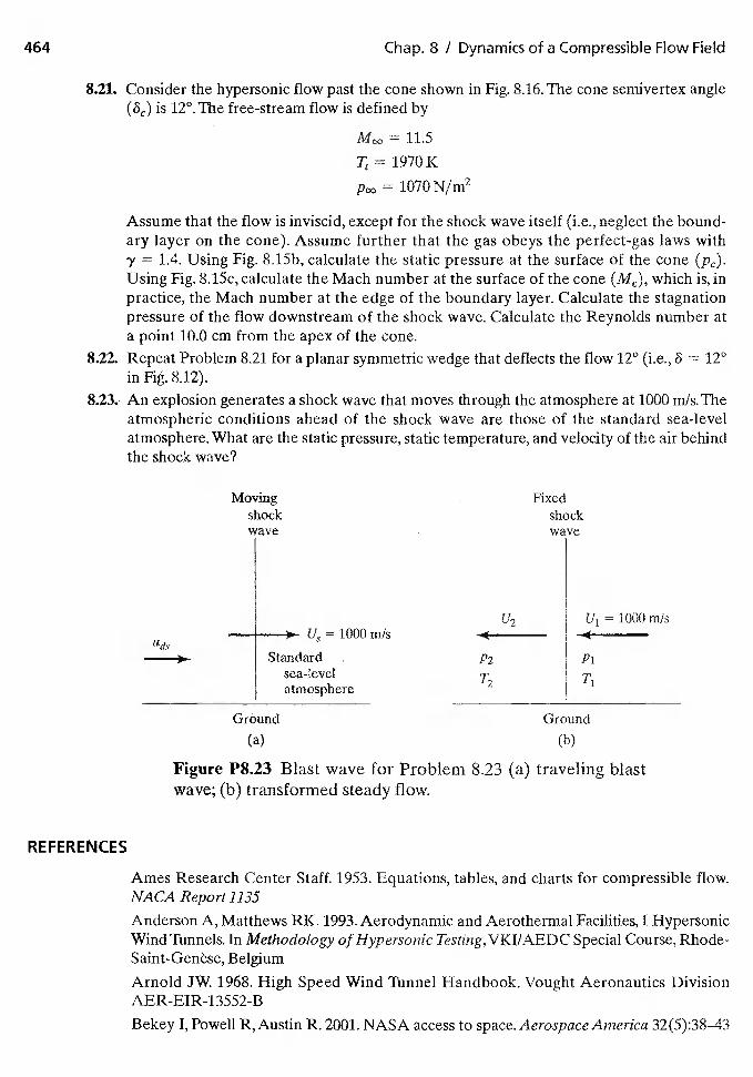
464 Chap. 8 / Dynamics of a Compressible Flow Field
8.21. Consider the hypersonic flow past the cone shown in Fig. 8.16. The cone semivertex angleis 12°.The free-stream flow is defined by
11.5
1970K
= 1070 N/rn2
Assume that the flow is inviscid, except for the shock wave itself (i.e., neglect the bound-ary layer on the cone). Assume further that the gas obeys the perfect-gas laws with
= 1.4. Using Fig. 8.15b, calculate the static pressure at the surface of the cone (Pc).Using Fig. 8.15c, calculate the Mach number at the surface of the cone (Me), which is, inpractice, the Mach number at the edge of the boundary layer. Calculate the stagnationpressure of the flow downstream of the shock wave. Calculate the Reynolds number ata point 10.0 cm from the apex of the cone.
8.22. Repeat Problem 8.21 for a planar symmetric wedge that deflects the flow 12° (i.e., 6 12°in Fig. 8.12).
An explosion generates a shock wave that moves through the atmosphere at 1000 m/s. Theatmospheric conditions ahead of the shock wave are those of the standard sea-levelatmosphere. What are the static pressure, static temperature, and velocity of the air behindthe shock wave?
Moving Fixedshock shockwave wave
U2 U1 = 1000 m/s— )
1tdsStandard P2
sea-levelatmosphere
Ground Ground
(a) (b)
Figure P8.23 Blast wave for Problem 8.23 (a) traveling blastwave; (b) transformed steady flow.
REFERENCES
Ames Research Center Staff. 1953. Equations, tables, and charts for compressible flow.NACA Report 1135
Anderson A, Matthews RK. 1993. Aerodynamic and Aerothermal Facilities, I HypersonicWind Tunnels. In Methodology of Hypersonic Testing,VKI/AEDC Special Course, Rhode-Saint-Genèse, Belgium
Arnold JW. 1968. High Speed Wind Tunnel Handbook. Vought Aeronautics DivisionAER-EIR-13552-B
Bekey I, Powell R, Austin R. 2001. NASA access to space. Aerospace America 32(5):38—43
References 465
Berry SA, Horvath TJ, Hollis BR, Thompson RA, Hamilton HH. 2001a. X-33 hypersonicboundary-layer transition. J. Spacecr. Rockets 38:646—657
Berry SA, Auslender H., Dilley AD, Calleja JF. 2001b. Hypersonic boundary-layer tripdevelopment for Hyper-X. J. Spacecr. Rockets 38:853—864
Bertin JJ. 1994. Hypersonic A erotherinodynamics. Washington, DC: AIAA
Bertin 11, Bouslog SA,Wang KC, Campbell CH. 1996. Recent aerothermodynamic flightmeasurements during Shuttle Orbiter re-entry. J. Spacecr. Rockets 33:457—462Berlin JJ, Cummings RM.2006. Critical hypersonic aerothermodynamic phenomena.Annu.Rev. Fluid Mech. 3 8:129—157
Buck ML, Benson BR, Sieron TR, Neumann RD. 1963. Aerodynamic and performanceanalyses of a superorbital re-entry vehicle. In Dynamics of Manned Lifting Planetary Entry,Ed. Scala SM, Harrison AC, Rogers M. New York: John Wiley
Buning PG, Wong TC, Dilley AD, Pao JL. 2001. Computational fluid dynamics predictionof Hyper-X stage separation aerodynamics. J. Spacecr. Rockets 38:820—827
Burcham FW, Nugent J. 1970. Local flow field around a pylon-mounted dummy ramjetengine on the X-15-2 airplane for Mach numbers from 2.0 to 6.7. NASA Tech. Note D-5638
Bushnell DM. 2006. Scaling: wind tunnel to flight. Annu. Rev. Fluid Mech. 36: 111—128
Chapman AJ. 1974. Heat Transfer. New York: Macmillan
Cockrell CE, Engelund WC, Bittner RD, Jentink TN, Dilley AD, Frendi, A. 2001. Integratedaeropropulsive computational fluid dynamics methodology for the Hyper-X flightexperiment. J. Spacecr. Rockets 38:836—843
Comette ES. 1966. Forebody temperatures and calorimeter heating rates measured duringproject Fire II reentry at 11.35 kilometers per second. NASA TMX-1 035Edney BE. 1968. Effects of shock impingement on the heat transfer around blunt bodies.AIAA J. 6:15—21.
Engelund WC. 2001. I-Iyper-X aerodynamics: The X-43A airframe-integrated scramjetpropulsion flight-test experiments. J. Spacecr. Rockets 38:801—802
Engelund WC, Holland SD, Cockrell CE, Bittner RD. 2001. Aerodynamic database devel-opment for the Hyper-X airframe-integrated scramjet propulsion experiments. .1. Spacecr.Rockets 38:803—810
Fujii K,Watanabe S,KurotakiT,Shirozu M. 2001.Aerodynamic heating measurements onnose and elevon of hypersonic flight experiment vehicle. J. Spacecr. Rockets 38:8—14
Hayes WD, Probstein RE 1966. Hypersonic Flow Theory, Vol. I, Inviscid Flows. New York:Academic Press
Hodge JK,Audley SR. 1983. Aerothermodynamic parameter estimation from shuttle ther-mocouple data during flight test maneuvers. J. Spacecr. Rockets 20:453—460
Holden M, Chadwick K, Kolly J. 1995. Hypervelocity studies in the LENS facility. Presentedat Intl. Aerosp. Planes Hypers.Tech. Conf., Pap. 95—6040, Chattanooga,TN
Holland SD, Woods WC, Engelund WC. 2001. Hyper-X research vehicle experimentalaerodynamics Ttest program overview. J. Spacecr. Rockets 38:828—835
Hollis BR, Horvath TJ, Berry SA, Hamilton HH,Thompson RA, Alter SJ. 2001a. X-33 com-putational aeroheating predictions and comparisons with experimental data. J. Spacecr.Rockets 38:658—669
Hollis BR,Thompson RA,Murphy KJ,Nowak RJ, Riley CJ, Wood WA,Alter SJ,Prabhu R.2001b. X-33 aerodynamic computations and comparisons with wind-tunnel data.J. Spacecr.Rockets 38:684—691
466 Chap. 8 / Dynamics of a Compressible Flow Field
Horvath TJ, Berry SA, Hollis BR, Liechty DS, Hamilton HH, Merski NR. 2001. X-33 exper-imental aeroheating at Mach 6 using phosphor thermography. .1. Spacecr. Rockets 38:634-645
Iliff KW, Shafer ME 1992. Space Shuttle hypersonic flight research and the comparison to groundtest results. Presented at Aerosp. Ground Test. Conf., 17th,AIAA Pap. 92—3988, Nashville, TN,
Kays WM. 1966. Convective Heat and Mass Transfer. New York: McGraw-Hill
Lee DB, Goodrich WD 1972. The aerothermodynamic environment of the Apollo Com-mand Module during suborbital entry. NASA Tech. Note D-6792
Matthews RK, Nutt KW,Wannenwetsch GD, Kidd CT, Boudreau AR 1985. Developmentsin aerothermal test techniques at the AEDC supersonic-hypersonic wind tunnels. Presentedat Thermophysics Conf., 20th, AIAA Pap. 85—1003, Williamsburg, VA
Moeckel WE, Weston KC. 1958. Composition and thermodynamic properties of air in chem-ical equilibrium. NACA Tech. Note 4265
Murphy KJ, Nowak RJ,Thompson RA, Hollis BR, Prabhu R. 2001. X-33 hypersonic aero-dynamic characteristics. J. Spacecr. Rockets 38:670—683
Neumann RD. 1988. Missions and requirements. AGARD Report 761, Special Course onAerothermodynamics of Hypersonic Vehicles, Neuilly sur Seine, France
Neumann RD. 1989. Defining the aerothermodynamic methodology. In Hypersonics,Volume I Defining the Hypersonic Environment, Ed. Bertin JJ, Glowinski R, Periaux J,Boston: Birkhaeuser BostonRied RC, Rochelle WC, Milhoan JD. 1972. Radiative heating to the Apollo Command Mod-ule: engineering prediction and flight measurements. NASA TMX-58091
Spalding DB, Chi SW. 1964. The drag of a compressible turbulent boundary layer on asmooth plate with and without heat transfer. .1 Fluid Mech. 18:117—143
Stalmach CJ. 1958. Experimental investigation of the surface impact pressure probe methodof measuring local skin friction at supersonic speeds. Defense Research Laboratory, TheUniversity of Texas at Austin, DRL-410
Sutton K. 1985. Air radiation revisited. In Progress in Astronautics andAeronautics Vol. 96:Thermal Design ofAeroassisted Orbiital Transfer Vehicles, Ed. Nelson HF, pp.419—441
Throckmorton DA. 1993. Shuttle entry aerothermodynamic flight research: the orbiterexperiments program. J. Spacecr. Rockets 30:449-465.
Throckmorton DA, Ed. 1995. Orbiter Experiments (OEX) Aerothermodynamics Sympo-sium. NASA CP3248
Trimmer LL, Cary AM,Voisinet RL. 1986.The optimum hypersonic wind tunnel, Presentedat Aerodyn. Test. Conf., l4th,AIAA Pap. 86—0739, West Palm Beach, FL
Wayland H. 1957. Differential Equations Applied in Science and Engineering, Princeton,NJ: Van Nostrand
Weston KC, Fitzkee AL. 1963. Afterbody heat transfer measurements obtained during reen-try of the spacecraft of the Mercury-Atlas 5 mission. NASA TM
Williamson WE. 1992. Hypersonic flight testing. Presented at Aerosp. Ground Test. Conf.,17th, AIAA Pap. 92—3989, Nashville, TN
Woods WC, Holland SD, DiFulvio M. 2001. Hyper-X stage separation wind-tunnel testprogram. J. Spacecr. Rockets 38:881—819
Wright RL, Zoby EV. 1977. Flight boundary layer transition measurements on a slendercone at Mach 20. at Fluid and Plasmadynarnics Conf., lOth,AIAA Pap. 77—0719,Albuquerque, NM
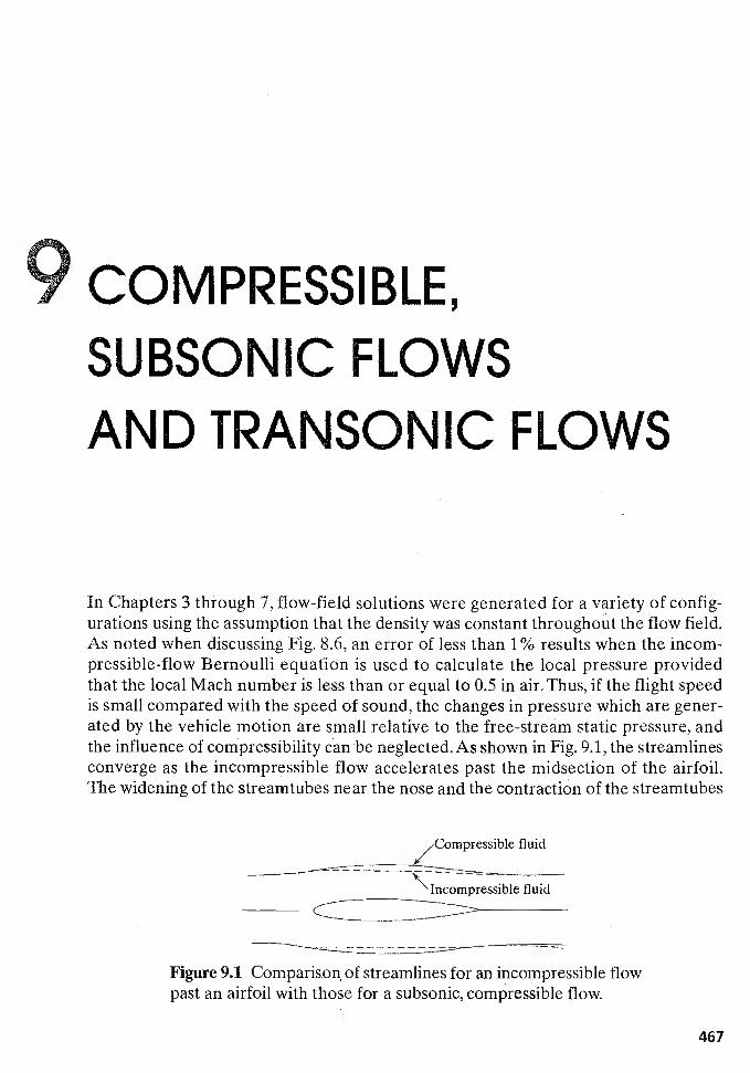
9 COMPRESSIBLE,
SUBSONIC FLOWS
AND TRANSONIC FLOWS
In Chapters 3 through 7, flow-field solutions were generated for a variety of config-urations using the assumption that the density was constant throughout the flow field.As noted when discussing Fig. 8.6, an error of less than 1% results when the incom-pressible-flow Bernoulli equation is used to calculate the local pressure providedthat the local Mach number is less than or equal to 0.5 in air. Thus, if the flight speedis small compared with the speed of sound, the changes in pressure which are gener-ated by the vehicle motion are small relative to the free-stream static pressure, andthe influence of compressibility can be neglected. As shown in Fig. 9.1, the streamlinesconverge as the incompressible flow accelerates past the midsection of the airfoil.The widening of the streamtubes near the nose and the contraction of the streamtubes
______
Incompressible fluid
Figure 9.1 Comparison of streamlines for an incompressible flowpast an airfoil with those for a subsonic, compressible flow.
467
468 Chap. 9 / Compressible, Subsonic FJows and Transonic Flows
in the regions of increased velocity lead to a progressive reduction in the curvatureof the streamlines. As a result, there is a rapid attenuation of the flow disturbance withdistance from the airfoil.
As the flight speed is increased, the flow may no longer be considered as incom-pressible. Even though the flow is everywhere subsonic, the density decreases as thepressure decreases (or, equivalently, as the velocity increases).The variable-density flowrequires a relatively high velocity and diverging streamlines in order to get the massflow past the midsection of the airfoil. The expansion of the minimum cross section ofthe streamtubes forces the streamlines outward so that they conform more nearly tothe curvature of the airfoil surface, as shown in Fig. 9.1. Thus, the disturbance causedby the airfoil extends vertically to a greater distance.
Increasing the flight speed further, we reach the critical Mach number, the namegiven to the lowest (subsonic) free-stream Mach number for which the maximum valueof the local velocity first becomes sonic. Above the critical Mach number, the flow fieldcontains regions of locally subsonic and locally supersonic velocities in juxtaposition.Such mixed subsonic/supersonic flow fields are termed transonic flows.
9.1 COMPRESSIBLE, SUBSONIC FLOW
For completely subsonic flows, a compressible flow retains a basic similarity to an incom-pressible flow. In particular, the compressible flow can be considered to be an irrotationalpotential motion in many cases. In addition to the absence of significant viscous forces, theexistence of potential motion for a compressible flow depends on the existence of a uniquerelation between the pressure and the density. In an inviscid flow, the fluid elements areaccelerated entirely by the action of the pressure gradient. Thus, if the density is a functionof the pressure only, the direction of the pressure gradient will coincide with that of thedensity gradient at all points.The force on each element will then be aligned with the centerof gravity of the fluid element and the pressure forces will introduce no rotation.
9.1.1 Linearized Theory for Compressible Subsonic FlowAbout.a Thin Wing at Relatively Small Angles of Attack
The continuity equation for steady, three—dimensiona' flow is
0(pu) + ±= (9.1)
0x
In the inviscid region of the flow field (i.e., outside the thin boundary layer), the com-ponents of the momentum equation may be written as
au au 1 apU— + V— + w— = (9.2a)
pax
lapU— + v— + w— = (9.2b)
8x 8y pay
0w 8w lapu— + v— + w— = (9.2c)0x äy az paz
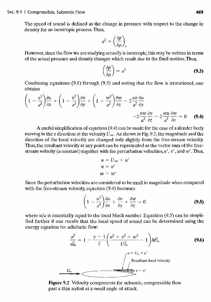
Sec. 9.1 / Compressible, Subsonic Flow 469
The speed of sound is defined as the change in pressure with respect to the change indensity for an isentropic process. Thus,
IsHowever, since the flow we are studying actually is isentropic, this may be written in termsof the actual pressure and density changes which result due to the fluid motion. Thus,
= (93)
Combining equations (9.1) through (9.3) and noting that the flow is irrotational, oneobtains
I I v2'\av I w2\aw uvau
\ a2) ax a2) ay \ a2) 3z a2 ay
— = 0 (9.4)a23z a23x
A useful simplification of equation (9.4) can be made for the case of a slender bodymoving in the x direction at the velocity As shown in Fig. 9.2, the magnitude and thedirection of the local velocity are changed only slightly from the free-stream velocity.Thus, the resultant velocity at any point can be represented as the vector sum of the free-stream velocity (a constant) together with the perturbation velocities, u', v', and w' . Thus,
U = Uco + U'
V =w=w,
Since the perturbation velocities are considered to be small in magnitude when comparedwith the free-stream velocity, equation (9.4) becomes
/ u2\öu av aw(1 ——1-----+—+—=o (9.5)\..
where u/a is essentially equal to the local Mach number. Equation (9.5) can be simpli-fied further if one recalls that the local speed of sound can be determined using theenergy equation for adiabatic flow:
(9.6)
U — + U'
Resultant local velocity
V
Figure 9.2 Velocity components for subsonic, compressible flowpast a thin airfoil at a small angle of attack.
470 Chap. 9 I Compressible, Subsonic Flows and Transonic Flows
Since only small perturbations are considered, the binomial theorem can be used togenerate the relation
= 1 + 1M2(2U + U'2 + v'2 + w12)
a
To simplify equation (9.5), note that
1a
(9.8) and neglecting the higher-order termsyields the expression
(9.9)
Using equation (9.9), equation (9.5) can be rewritten as
ax ay az 2
This equation can be rewritten in terms of the perturbation velocities as
(1 — + + + y— (9.10)
ax ay az 2 Ox
Furthermore, the term on the right-hand side often can be neglected, as it is of second orderin the perturbation velocity components. As a result, one obtains the linearized equation
au' 0V' 0w'(9.11)
0x 0y 0z
Since the flow is everywhere isentropic, it is irrotational. The condition of irrotational-ity allows us to introduce a velocity potential 4', which is a point function with continu-ous derivatives. Let be the potential function for the perturbation velocity:
U' = V' = w' = (9.12)ax Oy Oz
The resultant expression, which applies to a completely subsonic, compressible flow, isthe linearized potential equation
(1 — + cb)J), + = 0 (9.13)
By using a simple coordinate transformation, equation (9.13) can be reduced toLaplace's equation, which we used to describe incompressible, irrotational flows. If the"affine" transformation
x' = X(9.14a)
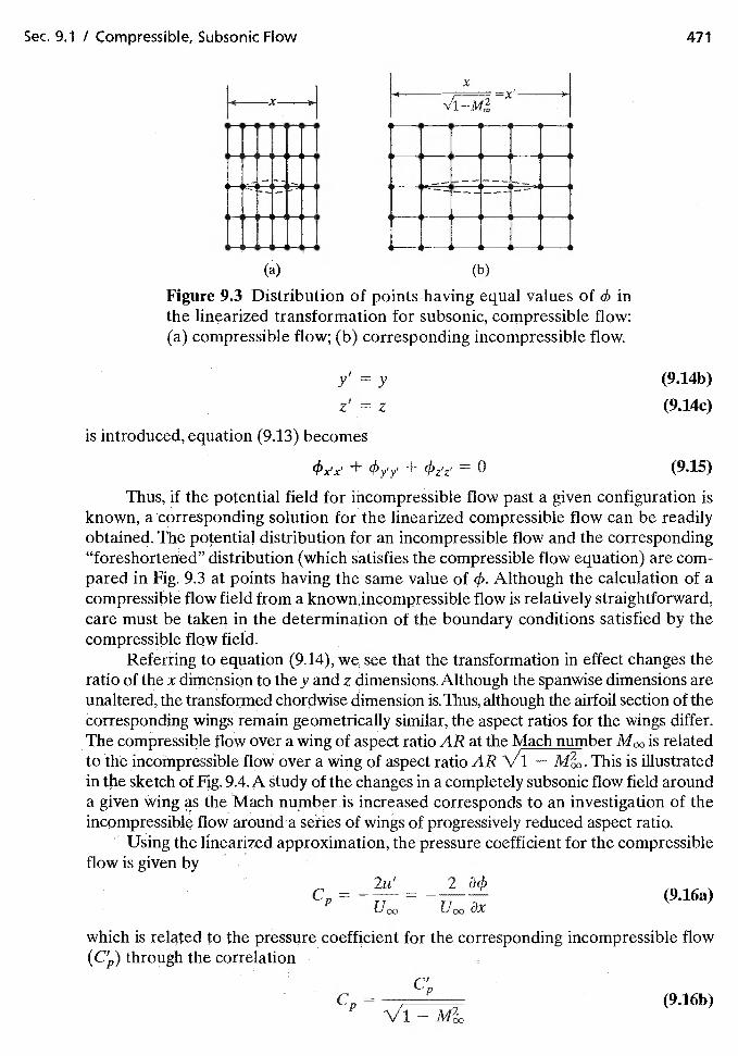
Sec. 9.1 I compressible, Subsonic Flow 471
x
x
(a) (b)
Figure 9.3 Distribution of points having equal values of 4) inthe linearized transformation for subsonic, compressible flow:(a) compressible flow; (b) corresponding incompressible flow.
y' = y (9.14b)
= z (914c)
is introduced, equation (9.13) becomes
+ + = 0 (9.15)
Thus, if the potential field for incompressible flow past a given configuration isknown, a corresponding solution for, the linearized compressible flow can be readilyobtained. The potential distribution for an incompressible flow and the corresponding"foreshortened" distribution (which the compressible flow equation) are com-pared in Fig. 9.3 at points having the same value of 4). Although the calculation of acompressible flow field from a known:incompressible flow is relatively straightforward,care must be taken in the determination of the boundary conditions satisfied by thecompressible flqw field.
Referring to equation (9.14), we see that the transformation in effect changes theratio of the dimension to they and z dimensions Although the spanwise dimensions areunaltered, the transformed chordwise dimension is. Thus, although the airfoil section of thecorresponding wings remain geometrically similar, the aspect ratios for the wings differ.The compressible flow over a wing of aspect ratio AR at the Mach number is relatedto the incompressible flow over a wing of aspect ratio AR This is illustratedin the sketch of Fig. 9.4. A study of the changes in a completely subsonic flow field arounda given wing as the'Mach number is increased corresponds to an investigation of theincompressiblà flow around a series Of wings of progressively reduced aspect ratio.
Using the linearized approximation, the pressure coefficient for the compressibleflow is given by
— — (9.16a)UOO&
which is related to the pressure coefficient for the corresponding incompressible flow(Ci,) through the correlation
(9.16b)

472 Chap. 9 / Compressible, Subsonic Flows and Transonic Flows
(a)
y
Figure 9.4 Wings for flows related by the linearized transforma-tion: (a) wing for compressible flow; (b) corresponding wing forincompressible flow.
The effect of compressibility on the flow past an airfoil system is to increase the hori-zontal perturbation velocities over the airfoil surface by the factor 1/\/1 — Thecorrelation is known as the Prandtl-Glauert formula.
We can calculate the lift by integrating the pressure distribution over the airfoil sur-face from the leading edge to the trailing edge. Based on equation (9.16b), we find that thesection lift coefficient for a compressible subsonic flow (C1) also exceeds the corresponding
2 0.5value for an incompressible flow (C1) by a factor of 1/[(1 — ]. Thus,
C'
The resultant variation for the lift-curve slope with Mach number is presented for atwo-dimensional unswept airfoil in Fig. 9.5.
dC,dcx
Figure 9.5 Variation of lift-curve slope1.0 with Mach number using Prandtl-Glauert
formula.
(b)
00.0 02 0.4 0.6 0.8
Mach number

Sec. 9.2 / Transonic Flow Past Unswept Airfoils 473
Furthermore, based on the pressure correlation of equation (9.16b), the positionof the resultant aerodynamic force for a compressible, subsonic flow is the same as thatfor an incompressible flow. This, of course, is true provided that there are no shock waves.Thus, in the absence of shock waves, the drag acting on an airfoil in an inviscid, compress-ible, subsonic flow is the same as the drag acting on an airfoil in an inviscid, incompressibleflow. That is, the section drag is zero.
Although the Prandtl-Glauert relation provides a simple method for calculatingthe flow around an airfoil, Jones and Cohen (1960) warn that the method generallyunderestimates the effect of compressibility on the magnitude of disturbances for air-foils of finite thickness. As the free-stream Mach number approaches a value of unity,the quantity 1/\/1 — approaches infinity, causing various perturbation parametersto approach infinity. Hence, the Prandtl-Glauert formula begins to show increasingdepartures from reality as the Mach number approaches a value of unity. The relativeinaccuracy at a particular Mach number depends on parameters such as the sectionthickness and the angle of attack.
Foss and Blay (1987) described a test flight of the YP-38 in September 1940. MajorSigna Gilkey peeled off into a steep dive starting at 35,000 ft. "As he headed down andthe airspeed built up, the airplane began to shake, mildly at first and then more vio-lently. Even worse, the airplane wanted to nose down further and increase the severityof the dive. The control column was shaking and the control forces had become heavy,and it was impossible to pull the column back to counteract the nose-down tendency. Theairplane was out of control!" As noted by Foss and Blay, Major Gilkey elected to staywith the plane and recovered at 7000 ft. "Major Gilkey had become the first pilot toencounter a new, uncharted high-speed flight regime. He had attained air speeds wherenew aerodynamic phenomena known as compressibility effects were created."
In seeking ways to control the aircraft experiencing these compressibility effects, thedesigners turned to the references of the time. Foss and Blay (1987) note, "In hindsight,it is interesting to note that no one was anticipating the nose down pitching moment ten-dencies, which were hinted at in section on pitching moment data. And of course,there were no data to suggest that hinge moments would become unmanageable."
Using a P-38 model in the high-speed wind tunnel of the Ames Research Center,model drag-rise characteristics were measured for the first time. The wind-tunnel cor-relations, as taken from Foss and Blay (1987), are reproduced in Fig. 9.6. Pressure dataand flow visualization clearly revealed the shock-stall conditions and helped confirmthe flight-test findings.
9.2 TRANSONIC FLOW PAST UNSWEPT AIRFOILS
The section lift coefficient measurements presented in Farren (1956) as a function ofMach number are reproduced in Fig. 9.7. The data indicate that the flow is essentiallyunchanged up to approximately one-third the speed of sound. The variations in the sec-tion lift coefficient with Mach number indicate complex changes in the flow field throughthe transonic speed range. Attention is called to the section lift coefficient at five par-ticular Mach numbers by the letters a through e). Significant differences existbetween the flow fields at these five Mach numbers. To illustrate the essential changesin the flow, line drawings made from schlieren photographs are reproduced in Fig. 9.8.

474 Chap. 9 / Compressible, Subsonic Flows and Transonic Flows
Lockheed; P-38Variation of Drag Coefficient with Mach Number
High-speed tunnel dataDrag CD A on 1/4 scale model
0.142
0.12 —
0.10 —
0
00.06
0.08
0.04
0.02 -.
0.2 0.4 0.6 0.8 1.0
Mach number
Figure 9.6 High-speed drag variation derived from wind-tunneltests. [From Foss and Blay (1987).]
CI
Figure 9.7 Section lift coefficient as a function of Mach numberto illustrate the effect of compressibility. [From Farren (1956).]Refer to Fig. 9.8 for the flow fields corresponding to the letteredpoints on this graph.
I I
Maximum CD assumedno data available toshow variation aboveM=0.83
Estimated above /this point

Sec. 9.2 / Transonic Flow Past Unswept Airfoils 475
Shocknow Wake 'Flow wave
(a) (b)
Flow Shock /1wave
Shockwave
(d)
Figure 9.8 Flow field around an airfoil in transonic streamsbased on schlieren photographs: (a) Mach number = 0.75;(b) Mach number = 0.81; (c) Mach number = 0.89;(d) Mach number = 0.98; (e) Mach number 1.4.[From Farren (1956).]
(a) When the free-stream Mach number is 0.75, the flow past the upper surfacedecelerates from local flow velocities which are supersonic without a shock wave.The section lift coefficient is approximately 60% greater than the low-speed valuesat the same angles of attack.
(b) At = 0.81, the section lift coefficient reaches its maximum value, which isapproximately twice the low-speed value. As indicated in Figs. 9.8b and 9.9a, flowis supersonic over the first 70% of the surface, terminating in a shock wave. Theflow on the lower surface is subsonic everywhere. Because the viscous flow sepa-rates at the foot of the shock wave, the wake is appreciably wider than for (a).
(c) At = 0.89, flow is supersonic over nearly the entire lower surface and decel-eration to subsonic speed through a shock wave at the trailing edge. As aresult, the lower surface pressures are lower at = 0.89 than at = 0.81.Flow on the upper surface is not greatly different than that for Fig. 9.8b. As a re-sult, the lift is drastically reduced. Separation at the foot of the upper surface shockwave is more conspicuous and the turbulent wake is wide. The shock wave at thetrailing edge of the lower surface effectively isolates the upper surface from thelower surface. As a result, the pressure on the upper surface near the trailing edgeis greater than that on the lower surface. The corresponding pressure and localMach number distributions are presented in Fig. 9.9b.
(d) When the free-stream Mach number is 0.98, the shock waves both for theupper surface and for the lower surface have reached the trailing edge. Thelocal Mach number is supersonic for most of the airfoil (both upper and lowersurfaces).
(e) When the free-stream flow is supersonic, a bow shock wave (i.e., the detachedshock wave in front of the leading edge) is generated.The flow around the airfoilis supersonic everywhere except very near the rounded nose. The shock waves atthe trailing edge remain, but they have become weaker.
The data presented in Figs. 9.7 through 9.9 illustrate the effect of Mach number fora given airfoil section at a particular angle of attack. Parameters such as thickness ratio,
(c)
(e)

C.)
C.)
0
476 Chap. 9 / Compressible, Subsonic Flows and Transonic Flows
pPrl
pPrl
1.00.0 0.5 1.0
xlc(a)
2.01.8
1.6
1.4
1.2
1.0
0.8
0.6
0.4
0.5
x/c(b)
Figure 9.9 Pressure distribution and local Mach number distrib-ution for transonic flows around an airfoil: (a) Flow at the trail-ing edge is subsonic, = 0.81; (b) flow at the lower surfacetrailing edge is supersonic, = 0.89. [From Farren (1956).]
camber, and nose radius also influence the magnitude of the compressibility effects.Transonic flows are very sensitive to the contour of the body surface, since changes inthe surface slope affect the location of the shock wave and, therefore, the inviscid flowfield as well as the downstream boundary-layer.

Sec. 9.2 I Transonic Flow Past Unswept Airfoils 477
Furthermore, as was discussed in Chapter 8, the shock-wave/boundary-layerinteraction and the possible development of separation downstream of the shock waveare sensitive to the character of the boundary-layer, to its thickness, and to its velocityprofile at the interaction location. Since a turbulent boundary-layer can negotiate higheradverse pressure gradients than can a laminar one, the shock-wave/boundary-layerinteraction is smaller for a turbulent boundary-layer. Thus, it is important to consider theReynolds number when simulating a flow in the wind tunnel. A large Reynolds numberdifference between the desired flow and its simulation may produce significant differ-ences in shock-wave location and the resultant flow field. The use of artificial trips toforce transition to occur at a specified point (as discussed in Chapter 5) may be unsat-isfactory for transonic flows, since the shock-wave location as well as the extent of flowseparation can become a function of the artificial tripping.
The Cobalt60 code [Strang, et a!. (1999)] has been used to compute the flow fieldaround a NACA 0012 airfoil section at an angle of attack of 3°. The turbulence model ofSpalart and Allmaras (1992) was used to represent the viscous boundary-layer near thesurface of the airfoil. Contours of constant Mach number, as computed by Forsythe andBlake (2000) for a free-stream Mach number of 0.8 at a free-stream Reynolds number(based on the chord length) of 3.0 X are presented in Fig. 9.10. The Mach 1 contoursfor the upper surface and for the lower surface are highlighted in white. Note that therelatively large area of supersonic flow on the upper surface is terminated by a shock
Figure 9.10 Constant-density contours for a NACA 0012 airfoil in a Mach0.8 stream at 3°. [As provided by Forsythe and Blake (2000).]

478 Chap. 9 / Compressible, Subsonic Flows and Transonic Flows
cp
wave at the downstream (or right-hand) side of the region of supersonic flow. The shockwave is evident in the sudden increase in pressure evident both in the experimental andin the computed pressure distributions for this airfoil, which are taken from Forsythe,et al. (2000) and reproduced in Fig. 9.11. The flow conditions for the experimental data,which are taken from Harris (1981), include a free-stream Mach number of 0.799, aReynolds number of 9.0 X 10⁶, and an angle of attack of 2.86°. The sudden increase inpressure due to the shock wave occurs on the upper surface at midchord.The adverse pres-sure gradient associated with the shock-wave/boundary-layer interaction causes theboundary layer to separate from the aft-end surface of the airfoil. This is evident in the(darkened region) Mach number contours presented in Fig. 9.10.
The section lift coefficient for this two-dimensional flow [Forsythe and Blake(2000)] is presented as a function of the free-stream Mach number in Fig. 9.12. Note thesimilarity between the Mach-number dependence of the computed section lift coefficient,as presented in Fig. 9.12, and that for the measurements presented by Farren (1956),which are reproduced in Fig. 9.7.
The computed flow field for transonic flow over a NACA 0012 airfoil that was pre-sented in Fig. 9.10 depicts regions (both above and below the airfoil) where the flow hasaccelerated to the point where the flow is locally supersonic. Since the pressure isdecreasing, the acceleration of the flow is often termed an expansion. During theisentropic expansion of the flow, there is a corresponding decrease in the temperature.
If the airplane is flying through an airstream where the relative humidity is high,the local temperature of the expanding flow can decrease below the dew point. Water
—1
—0.5
Experimental values as taken from Harris (1981)CFD (as provided by Forsythe and Blake (2000)
0.5
x/c
0.75 1
Figure 9.11 Pressure distributions for a NACA 0012 in a Mach 0.8stream at a = 3°.

Sec. 9.2 / Transonic Flow Past Unswept Airfoils 479
0.6
0.5
0.4
C1 0.3
0.2
0.1
00.5 1 1.5 2
Mach
Figure 9.12 Section lift coefficient for a NACA 0012 airfoil as afunction of the free-siream Mach number. [As provided byForsythe and Blake (2000).]
vapor will condense and become visible. Further downstream, as the flow decelerates(perhaps as it passes throtigh a shock wave that terminates the locally supersonic flow),the pressure and the temperature increase. As the local temperature rises above thedew point, the condensed particles evaporate (or vaporize) and are no longer visible.Thus, when an airplane is flying at transonic speeds in a relatively humid atmosphere,the relatively large accelerations (expansions) and decelerations (compressions) yielda condensation pattern, such as that for the F-151, which is presented in Fig. 9.13a.
The schlieren technique, which allows someOne to see shock waves in a wind-tunnel test, such as depicted on the cover and in Fig. 9.8, is based on density gradientsin the flow field that bend light rays passing through the flow. Under certain circum-stances, these density gradients allow us to "see" the shock waves for an airplane inflight, as shown for the transonic flight of an F-ill in Fig. 9.i3b.
The experimentally determined lift coefficients for an untwisted rectangular wingwhose aspect ratio is 2.75 and whose airfoil section is a NACA 65A005 (a symmetric pro-file for which t = 0.05c) are presented in Fig. 9.14 as a function of angle of attack. Thecorresponding drag polars are presented in Fig. 9.l5.These data from [Stahl and Mack-rodt (1965)] were obtained at Reynolds numbers between 1.0 X 10⁶ and 1.8 X 10⁶. Thelift-curve slope is seen to be a function of the free-stream Mach number. Furthermore,the linear relatiOn between the lift coefficient and the angle of attack remains valid tohigher angles of attack for supersonic flows.
IIII
0 CFD— — — — . Prandtl Glauert


Sec. 9.2 / Transonic Flow Past Unswept Airfoils 481
Subsonico = 0.39
= 0.78
o = 0.94
a, degrees
Figure 9.14 Effect of Mach number on the lift-coefficient/angle-of-attack correlation for a rectangular wing, AR 2.75. [Datafrom Stahl and Máckrodt (1965).]
Figure 9.15 Effect of the Mach number onI drag polars for a rectangular wing,
0.6 AR = 2.75. [Data from Stahl and Mack-rodt (1965).]
Supersonic
A 1.50
• Me.. = 2.25
1.6 —
1.2 -
CL 0.8 -
0.4 -
AA
A
0
0
a0
aOo•
00•0.0
0 8 16 24
Subsonicci = 039
Mor. = 0.78
Supersonic
•M= 1.50
A M,,= 2,25
CL
I •
1.2 -S•
A
••
A
I
0.4
0.0
—0.4 —0.0 0.2 0.4
CD

482 Chap. 9 / Compressible, Subsonic Flows and Transonic Flows
Bushnell (2004) noted: "shock waves are usually detrimental, re4uiring mitiga-The volume and lift-engendered drag associated with shock waves is additive to
the usual friction, and vortex drag-due-to-lift, comprising one-third of total aircraftdrag in the supersonic cruise case, even for the well-designed configuration. The rea-son for the decades-long Mach .8ish cruise-speed plateau associated with conventionallong-haul transport aircraft (requiring over ten hours of flight time transpacific) isavoidance of the major drag increases due to strong shock formation on the upperwing surfaces at higher speeds. Shock wave drag is also a major reason there are noeconomically viable supersonic transports yet extant. Due to wave drag, the aerody-riamic efficiency of a supersonic transport (SST) is the order of one-half or less of aconventional (subsonic) transport. Usual SST designs require a fuel fraction approaching60%, including reserves. A 1% overall drag reduction for these designs translates toa 5 to 10% increase in payload."
9.3 WAVE DRAG REDUCTION BY DESIGN
9.3.1 Airfoil Contour Wave Drag Approaches
Three features which contribute to the location of the shock wave and, therefore, to thepressure distribution [Holder (1964)1 are
1. The flow in the supersonic region ahead of the shock wave2. The pressure rise across the shock wave itself (which involves considerations of the
interaction with the boundary layer)
3. The subsonic flow downstream of the shock wave (which involves considerationsof the boundary-layer development between the shockwave and the trailing edgeand of the flow in the near wake)
If the trailing-edge pressure changes as a result of flow separation from the upper sur-face, the lower surface flow must adjust itself to produce a similar change in pressure(since the pressure near the trailing edge must be approximately equal for the two sur-faces, unless the flow is locally supersonic at the trailing edge). The conditions fordivergence of the trailing-edge pressure correspond to those for a rapid drop in the liftcoefficient and to the onset of certain unsteady flow phenomena, such as buffeting.
9.3.2 Supercritical Airfoil Sections
The Mach-number/lift-coefficient flight envelopes of modern jet aircraft operating attransonic speeds are limited by the compressibility drag rise and by the buffetingphenomenon. Airfoil section designs which alleviate or delay the onset of the drag riseand buffeting can contribute to higher maximum speeds (transport applications) or bet-ter lift performance (fighter applications). Using intuitive reasoning and substantiatingexperiment Whitcomb and Clark (1965) noted that R.T. Whitcomb and his coworkershave developed a "supercritical" airfoil shape which delays the subsonic drag rise. The

Sec. 9.3 / Wave Drag Reduction by Design 483
Supersonic flow
+
Weak shockwave
(b)
\\ IC
Figure 916 Comparison of transonic flow over a NACA 64Aseries airfoil with that over a "supercritical" airfoil section: (a)NACA 64A series, M 0.72; (b) supercritical airfoil, M = 0.80.[From Ayers (1972).]
principal differences between the transonic flow field for a conventional airfoil and thatfor a supercritical airfoil are illustrated by the data presented in Fig. 9.16. At supercrit-ical Mach numbers, a broad region of locally supersonic flow extends vertically fromboth airfoils, as indicated by the pressure coefficients above the sonic value and by theshaded areas of the flow fields in Fig. 9.16. The region of locally supersonic flow usuallyterminates in a shock wave, which results in increased drag. The much flatter shape ofthe upper surface of the supercritical airfoil causes the shock wave to occur downstreamand therefore reduces its strength.Thus, the pressure rise across the shock wave is reducedwith a corresponding reduction in drag. However, the diminished curvature of the uppersurface also results in a reduction of the lift carried by the midchord region of the air-foil section. To compensate for the loss in lift from the midchord region, additional liftmust be generated from the region of the airfoil behind the shock wave, particularly onthe lower surface. The increase of lift in this area is achieved by substantial positivecamber and incidence of the aft region of the airfoil, especially of the lower surface. Theincreased lift generated by the concave surface near the trailing edge of the lower sur-face is evident in the experimental pressure distributions presented in Fig. 9.17. The mid-chord region of the lower surface should be designed to maintain subcritical flow overthe range of operating conditions. If not, when the pressure rise associated with a shockwave is superimposed on the pressure rise caused by the cusp, separation of the lower-surface boundary-layer would occur. To minimize the surface curvatures (and, there-fore, the induced velocities) in the midchord regions both for the upper and the lowersurfaces, the leading-edge radius is relatively large.
Strong shock wave
Separated boundary
CI, CI,
+
(a)

484 Chap. 9 / Compressible, Subsonic Flows and Transonic Flows
I I0000 000 -
0
—0.6- -
o000o—0.4— 00 0 -
c(
—0.2- 0
0.0' 0' 0
0'0.2 -
a, a,0,0.4
0.6 -
0.8 I
0.0 0.2 0.4 0.6 0.8 1.0
x/c
Figure 9.17 Experimentally determined pressure distribution fora supercritical airfoil section, = 0.80, C1 = 0.54,
= 3.0 X 10⁶ (flagged symbols are for the lower surface).[Data from Hurley et al. (1975).]
9.4 SWEPT WINGS AT TRANSONIC SPEEDS
In the late 1930s, two aerodynamicists who had been taught by Prandtl, Adolf Buse-mann and Albert Betz, discovered that drag at transonic and supersonic speeds couldbe reduced by sweeping back the wings. [The interested reader is referred to Miller andSawers (1970)]. At the Volta conference in Rome in 1935, in his paper on high-speedflight, Busemann showed that sweepback would reduce drag at supersonic speeds. Betz,in 1939, was the first person to draw attention to the significant reduction in transonicdrag which comes when the wing is swept back enough to avoid the formation of shockwaves which occur when the flow over the wing is locally supersonic. The basic princi-ple is that the component of the main flow parallel to the wing leading edge is not per-turbed by the wing, so the critical conditions are reached only when the component ofthe free-stream velocity normal to the leading edge has been locally accelerated at somepoint on the wing to the local sonic speed. This simple principle is obviously only true(if at all) on an infinite span wing of constant section. Nevertheless, the initial sugges-tion of Betz led to wind-tunnel tests which substantiated the essence of the theory. The

Sec. 9.4 I Swept Wings at Transonic Speeds 485
CL
0.0 0.1 0.2 0.3
Figure 9.18 Comparison of the transonic drag polar for an unsweptwing with that for a swept wing. [Data from Schlichting (1960).]
results of the wind-tunnel measurements performed at Gottingen in 1939 by H. Ludwieg[as presented in Schlichting (1960)] are reproduced in Fig. 9.18. These data show that theeffect of the shock waves that occur on the wing at high subsonic speeds are delayed tohigher Mach numbers by sweepback.
The experimentally-determined lift coefficients and drag polars for a delta wingwhose aspect ratio is 2.31 and whose airfoil section is NACA 65A005 (a symmetric pro-file for which t = 0.05c) are presented in Fig. 9.19. These data from Stahl and Mackrodt(1965) were obtained at Reynolds numbers between 1.0 x 10⁶ and 1.8 X 10⁶. At sub-sonic speeds, the lift-coefficient/angle-of-attack correlation for the delta wing is markedlydifferent than that for a rectangular wing. (In addition to the data presented in Figs. 9.14and 9.19, the reader is referred to Chapter 7.) Even in subsonic streams, the lift is alinear function of the angle of attack up to relatively high inclinations. However, overthe angle-of-attack range for which the lift coefficient is a linear function of the angleof attack, the lift-curve slope (dCL/da) is greater for the rectangular wing for all thefree-stream Mach numbers considered.
One can use a variable-geometry (or swing-wing) design to obtain a suitable com-bination of low-speed and high-speed characteristics. In the highly swept, low-aspect-ratioconfiguration, the variable-geometry wing provides low wave drag and eliminates theneed for wing fold in the case of naval aircraft. At the opposite end of the sweep range,
—0.40.0
CD
0.1 0.2 0.3
CD

486 Chap. 9 I Compressible, Subsonic Flows and Transonic Flows
0.8CL
SubsonicD = 0.39
M,. = 0.78
a = 0.94
Supersonic= 1.50
= 2.25
Figure 919 Effect of Mach numberon the aerodynamic characteristics ofa delta wing;AR = 2.31, ALE 600:
(a) lift-coefficient/angle-of- attackcorrelation. [Data from Stahl andMackrodt (1965).]
one obtains efficient subsonic cruise and loiter and good maneuverability at the lowerspeeds. Negative factors in a swing-wing design are complexity, a loss of internal fuelcapacity, and the considerable weight of the hinge/pivot structure. A variable-geometrydesign, the Rockwell International Bi, is presented in Fig. 9.20.
9.4.1 Wing—Body Interactions and the "Area Rule"
The chordwise pressure distribution on a plane, finite-span, swept-back wing variesacross the span such that the maximum local velocity is reached much farther aft at theroot and farther forward at the tip compared to the basic infinite-wing distribution[Rogers and Hall (1960)].These distortions at the root and at the tip determine the flowpattern. On a swept wing with a square-cut tip, a shock wave first occurs near the tip. This"initial tip shock" is relatively short in extent. As the Mach number is increased, a rearshock is developed which dominates the flow. Because of the variation of the componentof velocity normal to the wing leading edge, streamlines over the wing surface will tendto be curved. However, the flow at the wing root is constrained to follow the fuselage.Therefore, for a straight fuselage, a set of compression waves originate in the wing-root
0 8
a, degrees
(a)
16 24

Sec. 94 / Swept Wings at Transonic Speeds 487
Subsonic Supersonico = 0.39 = 1.50
o = 0.94
F I
1.2- o0
0.8 - ah.
CL•
y
I I
0.0 0.2 0.4 0.6
CD
(b)
Figure (continued) (b) drag polar.
region to turn the flow parallel to the fuselage. As shown in Fig. 9.21, the compressionwaves propagate acrOss the wing span and ultimately may coalesce near the tip to formthe reat shock.
Thus, it is clear that the interaction between central fuselage and the sweptwing has a significant effect on the transonic flow over the wing. In the early 1950s,Kuchemann (1957> recognized that a properly shaped waistlike indentation on thefuselage could be designed to produce a velocity distribution on the wing near theroot similar to that on the corresponding infinite-span wing. KUchemann noted that"the critical Mach number can be raised and the drag reduced in the transonic and thesupersonic type of flow, the wing behaving in some respects like a thinner wing." Whit-comb (1954) found that the zero-lift drag rise is due primarily to shock waves. Fur-thermore, the shock-wave formations about relatively complex swept-wing/bodycombinations at zero lift near the speed of sound are similar to those which occur fora body of revolution with the same axial development of cross-sectional area normalto the airstream.Whitcomb concluded that "near the speed of sound, the zero-lift drag


Sec. 9.4 I Swept Wings at Transonic Speeds 489
Fuselage
I Initial positionof tip shock
Figure 9.21 Formation of rear shock from compression wavesassociated with flow near the root. [From Rogers and Hall (1960).]
fuselage and the wing) with axial position (as well as a reduction in the relative mag-nitude of the maximum area). Whitcomb noted that it would be expected that indentingthe body of a wing-body combination, so that the combination has nearly the sameaxial distribution of cross-sectional area as the original body alone, would result in alarge reduction in the transonic drag rise. Design applications of this "theory," whichis often known as area rule for trarisonic configurations, are illustrated inFig. 9.22. Early flight tests revealed that the prototypes of the YF-102 had seriousdeficiencies in performance. A major redesign effort included the first application ofWhitcomb's area rule to reduce the transonic drag. The modified YF-102A achievedsupersonic flight satisfactorily, providing the U.S. Air Force with its first operationaldelta-wing design. For additional information, the reader is referred to Taylor (1969).
The relation between the distribution of the cross-sectional area and the tran-sonic drag rise had a significant effect on the design of the Convair B-58, the Air Force'sfirst supersonic bomber. Free-flight, rocket-powered models of the original Convairdesign, designated MX-1626, were tested at the Wallops Island Flight Test Range(NAcA). The peak drag coefficient at Mach 1.02 was almost twice as high as that pre-dicted and the model did not achieve supersonic speeds. An evaluation of the longitu-dinal cross-sectional area distribution in accordance with the area rule of R. T. Whitcombalong with data obtained in the Helium Gun Facility at Wallops on a body of revolu-tion having the sam e longitudinal distribution of the cross-sectional area as the MX-1626 provided an explanation of the unexpectedly high drag. Presented in Fig. 9.23,which is taken from Shortal (1978), are a sketch of the planform of the MX-1626, thelongitudinal distribution of the cross-sectional area, and the drag coefficient for the
Approximatestreamlines
Compressionwaves
Rearshock

490 Chap. 9 / Compressible, Subsonic Flows and Transonic Flows
0UU,U,U,00
Figure 9.22 Application of the area rule to the axial distributionof the cross-sectional arca: (a) area rule applied to the design ofa near-sonic transport; (b) sketch of the Convair F 102 A. [FromGoodmanson and Gratzer (1973).]
Vehicle station(a)
(b)

Sec. 9.4 I Swept Wings at Transonic Speeds 491
(a) Original MX-1626 (b) PARD area rule design (c) Redesigned MX-1964
12
8
4
12
Total
12 X10' Wheel
8
4—Fuselage & pod
0 I I I ço 2 4 6 8 10x102
0.03 —
0.02
0.01 —
U
6
— XlO3esWing
Total
0 2 4 6 8 10 12X1020
0 2 4 8 10 12X102
I I I
0.03
0.02
0.01
00.9 1.0 1.1 1.2
0.03
0.02
0.01
00.8 0.9 1.0 1.1 1.2
C0
00.8 0.9 1.0 1.1 1.2
Mach number M M
Figure 9.23 Planform sketches, longitudinal distributions of cross-sectional areas, and drag coefficients for equivalent bodies of rev-olution for supersonic bomber models. [Taken from Shortal (1978).]
equivalent axisymmetric configuration as a function of the Mach number. Note how thewing, the wheel fairings, and the nacelles all add area to the fuselage and theweapons/fuel pod, creating a large total cross-sectional area. Furthermore, the place-ment of these components results in large longitudinal variations in the total cross-sectional area.
To reflect changes in the design requirements due to the unavailability of the orig-inally planned large jet engines and to changes in the function of the pod, the Air Forcechanged the Project Number from MX-1626 to MX-1964. R. N. Hopko, R. 0. Piland,and J. R. Hall set out to design a vehiële which met the general requirements of the newMX-1964 yet reduced the transonic drag rise. The design, designated PARD Area-RuleDesign in Fig. 9.23, included a 3% thick, 60-degree delta wing, modified by a 10-degreeforward swept trailing edge. The diamond-shaped wing provides a more gradual varia-tion in the cross-sectional area distribution. To this wing, they added four separatenacelles, staggered chordwise, and made the fuselage a body of revolution. The resultantplanform for the PARD Area-Rule Design, the longitudinal cross-sectional area distri-bution, and the measured drag coefficient for the equivalent body of revolution as afunction of the Mach number are reproduced in Fig. 9.23b.
Based on these data, Convair evaluated four alternative designs. Data for theconfiguration which had the lowest drag rise of the four Convair configurations are pre-sented in Fig. 9.23c. Note that the configuration designated the redesigned MX-1964

492 Chap. 9 / Compressible, Subsonic Flows and Transonic Flows
had both a smooth progression of cross-sectional area and the minimum value of themaximum cross-sectional area.
While touring the Air Force Museum at the Wright-Patterson Air Force Base, H.Hillaker (1994) noted, "The area-rule requirements of the B-58 required that the inboardand outboard nacelles be staggered —the inlet face of the outboard nacelle began on thesame plane as the exhaust face of the inboard nacelle. We previously had siamese nacelles(engines side-by-side as in a B-52 nacelle) which was lighter in weight but the higher dragmore than offset the lower weight." This is illustrated in the photograph of Fig. 9.24.
Applications of the area rule in the design of the F-S are illustrated in Figs. 9.25through 9.27. The benefit due to area ruling, considering a straight-sided fuselage as abase, is a large decrease in drag at transonic speeds, as shown in Fig. 9.25. As a result, thereis a corresponding increase in transonic acceleration, which is very important to thisfighter's design, since [According to Stuart (1978) and Bradley (1982)] the major anddecisive portions of air-to-air combat take place at altitudes below 30,000 ft at speedsfrom Mach 0.5 to 1.0.
Area ruling was also applied to the tip-tank design for the F-5A/B aircraft. Initialprototype flight and wind-tunnel tests indicated that transonic buffet and longitudinalinstabilities existed with the originally proposed wingtip tank. Continued developmenttests in the transonic wind tunnel proved that an area ruling concept (as shown in Fig. 9.26)could be used to essentially eliminate the pitch instabilities in the Mach 0.90 to 0.95region. A cruise drag benefit also existed because of the improvement in wing-tip air-flow characteristics. A slight instability which remained in the wind-tunnel data and wasthought to be Reynolds number dependent was never found during the flight tests. Thephotograph of an F5 (Fig. 9.27) illustrates these applications of the area rule.
Figure 9.24 Photograph of B-58. (From the collection of TIm Valdez.)

Mach no.
Figure 925 Reduction in the transonic drag rise due to the ap-plication of area rule to the F-S fuselage. [From Stuart (1978).]
By carefully designing the wing and the tail configurations, one can obtain a smoothvariation of the cross-section area even without adjusting the fuselage cross section.Such is the case for the swept-wing cruise missile which is presented in Fig. 9.28. Asshown in Fig. 9.29, the cross-section area distribution is relatively smooth and symmet-ric about the midbody station. This result is due, in part, to the high sweep angles for thewing and for the tail. As might be expected, this shape is conducive to low transonicdrag and the drag-rise Mach number is relatively high (i.e., approximately 0.95).Furthermore, the configuration could be trimmed with zero control deflection near thelift coefficient required for the maximum lift-to-drag ratio at a Mach number of 0.95.
Figure 9.26 Application of area rule to the design of the tip tankfor the F-5A/B aircraft. [From Stuart (1978)]
I I I I I
Sec. 9.4 / Swept Wings at Transonic Speeds 493
Drag
I I I I
0.2 0.4 0.6 0.8 1.0 1.2 1,4 1.6 1.8 2.0
CLUSE
= —0.0023
Cm()

494 Chap. 9 / Compressible, Subsonk Flows and Transonic Flows
9.4.2 Second-Order Area-Rute Considerations
Optimization of the wing/body/nacelle configuration plays a critical role in the designof business jets. Unlike previous business jets developed for cruising speeds near aMach number of 0.7, new aircraft are designed to cruise at speeds near Mach 0.8.Added to the requirement of more speed is the desire for significant increases in range.
Figure 9.28 Details of a model of a swept-wing cruise missile.Linear dimensions are in centimeters (inches). [From Spearmanand Collins (1972).]
Figure 9.27 Illustration of the application of the area rule to thetip tanks of the F-5. (From the author's collection.)
20.88(822)
50
5.03
Moment reference

Sec. 94 / Swept Wings at Transonic Speeds 495
xli
0.2
0.08
CD,o 0.04
0
12
(LID)max8
4
0
0.08
CL
I) 0.4 0.8 1.2 L6 20 2.4 2.8 3.2
Figure 9.29 Area distribution and various aerodynamic parame-ters for a swept-wing cruise missile. [From Spearman and Collins(1972).]
To meet these requirements, the designs employ wings with more sweep and careful-iy designed cross sections that minimize the onset of the compressibility drag. Fur-thermore, these high-speed wings must be compatible with typical business jetconfigurations that have engines mounted on the fuselage near the wing trailing edge.As noted by Galiman, et at (1996). "These requirements create an aerodynamic designproblem that benefits from modern computational fluid dynamics (CFD) and aero-dynamic shape optimization.. . . Full potential analysis of the wing-body-nacelle con-figuration provided an accurate assessment of the influence of the fuselage mountedengines on wing pressures." Galiman, et al. (1996) used codes similar to those discussed(briefly) in Chapter 14.
The area rule is essentially a linear-theory concept for zero lift. Whitcomb(1976) noted that "to achieve the most satisfactory drag characteristics at liftingconditions the fuselage shape had to. be modified from that defined by the simpleapplication of the area rule as previously described to account for the nonlinearity
Cross-sectional o.i
area
0
\%
— —
(1_-__

496 Chap. 9 / Compressible, Subsonic Flows and Transonic Flows
00'U0,02
0C.-)
Figure 9.30 Second-order area rule considerations. [FromWhitcomb (1976).]
of the flow at such conditions. For lifting conditions at near sonic speeds there is asubstantial local region of supercritical flow above the wing surface which results inlocal expansions of the streamtube areas. In the basic considerations of the arearule concept, this expansion is equivalent to an increase in the physical thickness ofthe wing. To compensate for this effect the fuselage indentation required to elimi-nate the far-field effects of the wing must be increased." The additional correctionto the cross-sectional areas required for a transonic transport, as taken from Whit-comb (1976) is illustrated in Fig. 9.30. "The fuselage indentation based on thiscorrected cross-sectional area distribution resulted in a significant delay in thedrag rise Mach number compared with that for the indentation based on the zerolift distribution."
However, as noted by Ayers (1972), the fuselage cross-sectional area needed forstoring landing gear and aircraft subsystems and for accommodating passenger seatingand headroom, conflicts with the area-rule requirements in some cases.
Carlsen (1995) noted: "That the sonic area rule is a far field method of predictingand understanding the wave drag due to shock losses [Whitcomb (1956)]. It is based onthe idea of perfect pressure disturbance communication between the wing, or otherexternal features, and the fuselage. It proposes that a body of revolution with the sameaxial development of cross-sectional area will have a wave drag that is similar to theoriginal configuration [Whitcomb (1956)].
Carisen (1995) noted that the communication between the flow on the wing andthe flow on the fuselage changes in the transonic regime because of the mixed supersonicand subsonic flow. "In transonic flow, dissipation of disturbances occurs in the subson-ic regions and the stream-tube areas are no longer invariant. As a result of this dissipa-tion, it is erroneous to subtract the total wing volume from the fuselage. Part of thepressure changes created by the indentations in the fuselage is dissipated before it reach-es the wing by passing through embedded subsonic regions. To account for the majori-ty of this dissipation, the new transonic method applies a weighting function to the sonicarea rule that modifies the volume removed from the fuselage. Only the volume that will
Vehicle station

Sec. 9.4 / Swept Wings at Transonic Speeds 497
relieve the flow on the wing should be removed. This minimizes the volume removedfrom the fuselage and still maintains the drag rise delay."
Carisen (1995) recommended the use of weighting functions that would be applied"during the integration of the area of the wing that is intersected by a given Mach 1plane. Area at the wingtip is given less value than the area near the wing root. The weight-ed wing area is then subtracted from the fuselage area that is intersected by this sameMach plane. The procedure is repeated at. a series of locations along the fuselage axis,resulting in a net volume removal from the fuselage."
Carisen (1995) concludes that the proposed use of a weighting function adjustsfor the effects of mixed flows, i.e., the communication between the flow over the fuse-lage and that over its external parts that accounts for the dissipation due to embeddedsubsonic regions. The dissipating effect of the subsonic regions in the transonic regimesignificantly influences the approach to area ruling. Drag-rise delays that match the tra-ditional sonic-area-rule can be obtained by modifying the aircraft to only 60% of whattraditional sonic-area-rule prescribes.
9.4.3 Forward Swept Wing
The aerodynamic effects (e.g., increased critical Mach number, decreased lift curve slope,etc.) resulting from wing sweepback are also present for forward swept wings (FSW) aswell. However, there are some comparative advantages to a FSW in relation to an aftswept wing (ASW), which will be discussed in this section.
Historically, the use of FSW in aircraft designs was, with minor exceptions, pre-cluded by the relatively low (in comparison with ASW) Mach numbers at which theyexperience aeroelastic flutter and divergence when, they are constructed of conven-tional aircraft materials such as metals. The reasons for this will be discussed later,but, as an example, Diederich and Budiansky (1948) show that uniform FSWs withsweep angles from —20 to —60° exhibit decreases as high as 78% in aeroelastic di-vergence dynamic pressures in comparison to straight wings. To eliminate this prob-lem using conventional materials requires a prohibitive structural weight penalty. Thus,until recently, the FSW, along with some of its desirable characteristics, has beenexcluded from the aircraft designer's stable of design options. However, recent ad-vances in the development of composite materials for aircraft structures have per-mitted the design and fabrication of aeroelastically tailored wings which substantiallyeliminate the divergence problem.
A swept wing constructed of conventional materials twists under load. AnASW twists down at the tips as the lift increases while a FSW twists up. In the for-mer case, the tips tend to unload, while in the latter case they tend to load the struc-ture further. Thus, the FSW constructed of conventional materials has a much lowerspeed for structural divergence which occurs when the elastic restoring forces canno longer overcome the aerodynamic forces causing the deformation. The twistingbehavior occurs because the axis of section centers of pressure along the span of anASW is behind the structural axis of the wing in typical designs, while just theopposite is true for the FSW [Uhuad, et al. (1983)].The structural axis can be thoughtof as the locus of points along the wing where a load produces only wing bendingwith no twist.

498 Chap. 9 / Compressib'e, Subsonic Flows and Transonic Flows
The solution to this problem for the FSW is to design an aeroelastically tailored wingusing composite materials arranged in unidirectional layers or plies which lie at selected an-gles relative to one another. By careful design and fabrication, the wing can be made todeform under loading so that the divergence problem just described can be delayed to amuch higher Mach number. This permits the designer to capitalize on some of the advan-tages of FSWs compared toASWs without paying an exhorbitant weight penalty. Inciden-tally, aeroelastic tailoring is not limited to FSWs, but can be applied to straight and aft sweptwings as well [Brown et al. (1980)].
The relative advantages of the FSW over the ASW are, of course, a function ofthe aircraft mission and fall into aerodynamic and other categories. Excellent overalldiscussions of these FSW characteristics are given in Whitford (1987) and in Krone(1980). We restrict our discussion here to aerodynamic advantages of the FSW. Keyaerodynamic advantages of the FSWfall into two categories: reduced drag and enhancedmaneuverability at transonic Mach numbers and high angles-of-attack.
Modem aircraft designs rely on wing sweep and supercritical airfoil sections todelay adverse compressibility effects and reduce their severity when they do occur.Good design practices force the shock on the upper surface of the wing to occur asclose to the trailing edge as possible and to be as weak as possible. Typical shocklocations for a supercritical wing occur in the vicinity of the 70% chord line along thespan. As noted by Whitford (1987), this results in a more highly swept shock for anFSW compared to an ASW with the same leading-edge sweep angle, wing area, andtaper ratio. The more highly swept shock, of course, results in a lower wave dragpenalty. Further, for designs with the same shock sweep angle, the FSW requires lessleading-edge sweep, which resUlts in a higher lift curve slope than the comparableASW and a reduction in induced drag at subsonic conditions. And although the lowerleading-edge sweep will result in higher wave drag at supersonic conditions, drag dueto shock-induced separation has been found to be less. Thus, as noted earlier, carefulattention to the aircraft mission will determine the design solution to be adopted ineach case. Whitford (1987) also points out that an FSW with the same planform area,shock sweep, and span as an ASW has its aerodynamic center closer to the wing rootand hence experiences a lower wing root bending moment. Conversely, an FSW can bedesigned with a higher aspect ratio than a comparable ASW and produce the same bend-ing moment at the wing root.The higher aspect ratio in turn produces lower induced drag.
Flow over an ASW has a component along the span and toward the tips whichresults in a thicker boundary layer in the tip region than would otherwise exist. This,coupled with the more highly loaded tips of the ASW, can lead to tip stall, with the stallregion moving inward toward the root as the stall progresses. This phenomenon can re-suit in loss ofaileron control effectiveness at high angles-of-attack with a consequent lossof maneuverability. An additional and undesirable offshoot of thisphenomenon is anoverall pitch-up tendency since the loss of lift typically occurs aft of the aircraft centerof gravity. For the FSW the spanwise flow component is toward the wing root leadingto root stall first. Thus, aileron effectiveness is preserved up to higher angles-of-attackwith a consequent improvement in maneuverability. However, the FSW with root stallstill suffers the pitch-up tendency since the loss of lift is once again typically aft of theaircraft center of gravity.

Sec. 9.4 / Swept Wings at Transonic Speeds 499
Nose strake
Figure 9.31 Three-view sketch of full-scale X-29 configuration.
To investigate further and to validate by flight test these and other potential ad-vantages of the FSW relative to the ASW, the Defense Advanced Research ProjectsAgency (DARPA), NASA, and the Air Force have funded the design and fabrication ofthe X-29. This aircraft, produced by Grumman, is an experimental flight-test vehicledesigned to explore a variety of advanced technologies, including FSW and close-coupled canards. The primary objective of the X-29 program is to give designers confidencein the FSW approach and to validate the advantages of FSW and other technologiesfor use in future aircraft designs [Putnam (1984)].
The X-29 configuration, illustrated in the three view sketches of Fig. 9.31, hasseveral distinctive design features. These include a three-surface longitudinal controldesign, consisting of an all-movable close-coupled canard with large deflection capa-bility, symmetric deflection of wing flaperons, and deflectable aft-fuselage strake flaps.Roll control is provided by differential flaperon deflection (or, equivalently, ailerondeflection). A conventional rudder provides directional control. The X-29 has a longslender forebody, similar to the F-5 design, which produces strong vortical flow in thestall/poststall region.
Using data obtained in free-flight wind-tunnel tests at the Langley ResearchCenter (NASA), Croom et al. (1988) studied the low-speed, high-angle-of-attack flightdynamics of the X-29 configuration. As noted by Croom et al. (1988), "The most dom-inant characteristic of the configuration is the extreme level of inherent static pitchinstability (—0.35 static margin). Clearly, the basic airframe is unflyable without sta-bility augmentation. However, the all-movable canard and strake flap control surfacesprovide significant control authority throughout the trim angle-of-attack rangeMoreover, the large control moments in conjunction with the relatively low pitch in-ertia, associated with the relatively lightweight design indicate the potential for a highlevel of pitch agility, which is very desirable for fighter aircraft."
A major benefit arising from the use of forward-swept wings at high angles-of-attack is the favorable progression of the stall pattern. Flow separation progresses from
Flaperon
Strake
strake

500 Chap. 9 / Compressible, Subsonic Flows and Transonic Flows
the wing-root region outboard, resulting in the retention of aileron control power beyondthe stall angle-of-attack.Thus, significant roll control moments persist to very high anglesof attack and lateral control should be comparatively good throughout the trim angle-of—attack range.
As noted by Croom et al. (1988) "The data show good levels of static directional sta-bility below 20-deg. angle of attack. However, as the angle of attack is increased above25-deg., the directional stability degrades significantly, resulting in unstable to neutrallystable values for trim canard incidences. The reduction in stability is due to the verticaltail becoming immersed in the low energy wake of the wing. However, at poststall anglesof attack, the directional stability is re-established. Past studies have shown that undersideslip conditions, the flat elliptical cross-section forebody generates an asymmetric vor-tex system that produces a suction force on the windward side of the forebody resultingin yawing moments into the sideslip (i.e., stabilizing)."
9.5 TRANSON1C AiRCRAFT
Ayers (1972) also notes that "wind-tunnel studies have indicated that combining thesupercritical airfoil, the area rule, and wing sweep can push the cruising speed ofsubsonic aircraft very near Mach 1.0." Using computer-oriented numerical tech-niques, numerous investigators have solved the nonlinear equation for the distur-bance velocity potential in transonic flow, which can be written [refer to Newman andAllison (1971)]
(1 — + + 4,, = (9.17)
Comparing equation (9.17) with equation (9.10), one would find that, for the particularassumptions made during the development of equation (9.10),
In the transonic Mach number range, this term cannot be neglected as it was at lowerspeeds; see equation (9.10).
Bailey and Ballhaus (1975) used a relaxation procedure to solve the transonicsmall-disturbance equation:
(1 — + += 1
(9.18)
The parameter n reflects the nonuniqueness of the equation and, quoting Bailey andBallhaus (1975), "can be adjusted to better approximate the exact sonic pressurecoefficient." A finite-difference equation is derived by applying the divergence the-orem to the integral of equation (918) over an elemental, rectangular, computationvolume (or cell). The boundary conditions for the wing include the Kutta condition,which requires that the pressure, which is proportional to be continuous at thetrailing edge. This fixes the section circulation, which is equal to the difference in

Sec. 9.5 I Transonic Aircraft 501
CF
Figure 9.32 Comparison of computed and experimental pressurecoefficients for swept-wing/fuselage configuration, = 0.93;a = 0°, A = 0.6, NACA 65A006 streamwisesection. [From Bailey and Balihaus (1975),]
potential at the section trailing edge linearly extrapolated from points above andbelow. The solution of the difference equation is obtained by a relaxation schemewith the iterations viewed as steps in pseudo-time. The combination of new and oldvalues in the difference operators is chosen so that the related time-dependent equa-tion represents a properly posed problem whose steady-state solution approachesthat of the steady-state equation. The calculated and the experimental pressure dis-tributions for a swept-wing/fuselage configuration at = 0.93 and a = 0° are com-pared in Fig. 9.32. The wing has an aspect ratio of 4 and a taper ratio of 0.6. Thequarter chord of the wing is swept 45° and the strearnwise airfoil section is a NACA65A006. The computed results were obtained using a Cartesian grid (x, y, z) of91 X 59 x 27 for the wing as well as for the fuselage. The experimental data wereobtained at = 2.0 x 10⁶. As was noted earlier in this chapter, the maximumvelocity is reached farther aft forthe stations near the root and moves toward theleading edge at stations nearer the tip. The agreement with experiment on the fuse-lage centerline and the two inboard panels is good. In the computed results, the wing-root shock propagates laterally to 2y/b 0.60, but the experimental shock dissipatesbefore reaching that point. Thus, there is a discrepancy between the experimentalvalues and the theoretical predictions. This deficiency results for wings with moder-ate-to-large sweep angles. Balihaus, Bailey, and Prick (1976) note that a modifiedsmall-disturbance equation, containing cross-flow terms which have been previous-ly neglected, would be a suitable approximation to the full potential equation over awide range of sweep angles. Thus, a small-disturbance differential equation whichcould be used to describe the resultant three-dimensional flow is
—0.4
—0.4 2yIb = 0.95
—0.4
—0.2
2yIb = 0.80
2y/b = 0.60
2y/b 0.40
2y/b = 0.20

502 Chap. 9 I Compressible, Subsonic Flows and Transonic Flows
(1 — ± + — ('y +
o'I-'y+'xy I Y )' 2
lvi cY31-'X+'XX
Note that the terms on the left-hand side of this equation are those of equation(9.18) and those on the right-hand side are the additional terms of the modified small-disturbance formulation. Boppe (1978) notes that the cross-flow terms, and
provide the ability to define shock waves which are swept considerably relativeto the free-stream flow. Boppe recommends that the higher-order term, be includedto provide an improved approximation to the full potential equation at the critical velocity.Ballhaus et a!. (1976) note that the use of an improved form of the governing equationalone does not guarantee that the shock waves will be properly represented. The finite-difference scheme must also adequately describe the physics of the problem.
Flow-field solutions for complex airplane configurations flying at transonic speedscan be computed using numerical programs that solve the Euler equations. The Eulerequations for three-dimensional flows are presented in Appendix A. Using a structured,surface-fitted grid, et al. (1987) generated solutions for the flow over advancedturboprop (with an ultra-high-bypass propulsion system) airplane configurations. Astructured surface-fitted grid on the configuration surface, as shown in Fig. 9.33, was
Figure 9.33 Structured surface-fitted grid for an advanced prop-fan airplane. [From Kusunose et 2il. (1987) .1

Problems 503
generated first and then the flow-field grids were obtained using an elliptic grid gen-eration scheme. Kusunôse et a!. (1987) chose this scheme because it offered "twomajor advantages: (1) the structural grid requires minimum storage for the flow solu-tion since the grid points are well ordered and (2) the surface-fitted grid allows eas-ier and more accurate implementation of the boundary conditions." The presence oftrailing vortex wakes produced by the wing, the strut, and the horizontal tail as wellas the slip-stream and 'the rotational flow (with different total pressure and total tem-perature) produced by the propellor led Kusunose et ai. (1987) to use the Euler equa-tions in formulating the solution algorithm. "When these are solved, trailing vortexwakes come out automatically as part of the solution, and the rotational flows arecaptured naturally through the Euler equation formulation." To account for the vis-cous effects on the wing, the Euler solver is coupled with a three-dimensional boundary-layer method McLean et a!. (1978). For the approach of Kusunose et al. (1987) theviscous effects are simulated by using the boundary-layer displacement thickness tocreate an effective "displacement body." Miranda (1984) indicates that modifying theboundary condition (i.e., the surface transpiration concept) is preferable to the dis-placement body approach because the surface geometry and the computational gridare 'not affected by the boundary layer.
Miranda (1984) notes that the problem of grid generation is a crucial one for thepractical application of numerical flow simulation. Both methods of solution, singular-ity and field, require the construction of complex computational grids: mesh-surfacegrids for singularity methods andspatial grids for field methods.
SUMMARY
Transonic flows are inherently nonlinear and highly three dimensional for wing-bodycombinations. The nonlinear inviscid flow and the resultant shock waves present aconsiderable challenge to the analyst. Strong shock-wave/boundary-layer interactionscause rapid increases in drag and can lead to buffeting. Shock-induced boundary-layerseparation can also limit the lift coefficient. However, experimental investigations haveprovided considerable insights into desirable design practices for transonic configura-tions. Furthermore, three-dimensional transonic flow computational techniques aredeveloping at a rapid pace.
PROBLEMS
9.1. Starting with the energy equation for steady, one-dimensional, adiabatic flow of a perfectgas [i.e., equation (8.29)], derive equation (9.7).
9.2. 'A rectangular wing having an aspect ratio of 3.5 is flying at = 0.85 at 12 km. A NACA0006 airfoil section is used at all spanwise stations. What is the airfoil section and the aspectratio for the equivalent wing in an incompressible flow?
9.3. When discussing Whitcomb's area rule, it was noted that, for lifting conditions, there is asubstantial local region of supercritical flow above the wing surface which results in localexpansions of the streamtube areas. Consider flow past a two-dimensional airfoil in a streamwhere = 0.85. Calculate the distance between two streamlines, dye, at a point where

504 Chap. 9 / Compressible, Subsonic Flows and Transonic Flows
the local inviscid Mach number, Me, is 1.20 in terms of the distance between these twostreamlines in the undisturbed flow, Use the integral form of the continuity equation[equation (2.5)],
dYe =
Assume an isentropic expansion of a perfect gas.
REFERENCES
Ayers TG. 1972. Supercritical aerodynamics: worthwhile over a range of speeds. Astronaut.Aeronaut. 10(8):32—36
Bailey FR, Ballhaus WF. 1975. Comparisons of computed and experimental pressuresfor transonic flows about isolated wings and wing-fuselage configurations. NASA Spec.Pub. 347
Ballhaus WF, Bailey FR, Frick 11976. Improved computational treatment of transonic flowabout swept wings. NASA Conf Proc. 2001
Boppe CW. 1978. Computational transonic flow about realistic aircraft configurations.Presented at AIAA Aerosp. Sci. Meet., 16th AIAA Pap. 78—104, Huntsville, AL
Bradley RG. 1982. Practical aerodynamic problems—military aircraft. In TransonicAerodynamics. Ed Nixon D,Washington, DC:AIAA
BrowniE, Price MA, Gringrich PB. 1980. Aeroelastically tailored wing design. Presentedat The Evolution of Wing Design Symp.,AIAA Pap. 80—3046, Dayton, OH
CarlsenWD. 1995. Development of transonic area-rule methodology. J.Aircraft 32:1056—1061
Croom MA, Whipple RD, Murri DG, Grafton SB, Fratello DJ. 1988. High-alpha flightdynamics research on the X-29 configuration using dynamic model test techniques.Proceedings of the Aerosp. Tech. Conf., SAE Pap. 881420, Anaheim, CA
Diederich FW, Budiansky B. 1948. Divergence of swept wings. NACA Tech. Note 1680
Farren WS. 1956. The aerodynamic art. J. Roy. Aero. Soc. 60:431—449
Forsythe JR, Blake DC. 2000. Private Transmittal
Forsythe JR, Strang WZ, Hoffmann KA. 2000. Validation of several Reynolds averagedturbulence models in a 3-D unstructured grid code. Presented at AIAA Fluids 2000 Conf.,AIAA Pap. 2000—2552, Denver, CO
Foss RL, Blay R. 1987. From propellers to jets in fighter aircraft design. Lockheed Horizons23:2—17
Gailman JW, Reuther JJ, Pfeiffer NJ, Forrest WC, Bernstorf DJ. 1996. Business jet wingdesign using aerodynamic shape optimization. Presented at AIAA Aerosp. Sci. Meet., 34th
AIAA Pap. 96—0554, Reno, NV
Goodmanson LT, Gratzer LB. 1973. Recent advances in aerodynamics for transport aircraft.Aeronaut. Astronaut. 11(12):30—45
Harris CD. 1981.Two-dimensional aerodynamic characteristics of the NACA 0012 airfoil inthe Langley 8-foot transonic pressure tunnel. NASA Tech. Mem. 81927

References 505
Hillaker H. 1994. Private Conversation
Holder DW. 1964. The transonic flow past two-dimensional aerofoils. J. Roy. Aero. Soc.68:501—516
Hurley FX, Spaid FW, Roos FW, Stivers LS, Bandettini A. 1975. Detailed transonic flowfield measurements about a supercritical airfoil section. NASA Tech. Mem. X-3244
Jones RT, Cohen D. 1960. High Speed Wing Theory. Princeton NJ: Princeton UniversityPress
Krone NJ. 1980. Forward swept wing design. Presented at The Evolution of Wing DesignSymp.,AIAA Pap. 80—3047, Dayton, OH
KUchemann D. 1957. Methods of reducing the transonic drag of swept-back wings at zerolift. J. Roy.Aero. Soc. 61:37—42
Kusunose K, Mascum DL, Chen HC,Yu NJ. 1987. Transonic analysis for complex airplaneconfigurations. Presented at AIAA Fluid Dyn.,Plasma Dyn., and Lasers Conf., 19th AIAAPap. 87—1196, Honolulu, HI
McLean JTD, Randall JL. 1978. Computer program to calculate three-dimensional boundary-layer flows over wings with wall mass transfer. NASA Contr. Rep. 3123
Miller R, Sawers D. 1970. The Technical Development of Modern Aviation. New York:Praeger Publishers
Miranda LR. 1984. Application of computational aerodynamics to airplane design. J. Aircraft21 :355—370
Newman PA,Allison p0.1971. An annotated bibliography on transonic flow theory. NASATech. Mem. X-2353
Putnam TW. 1984. The X-29 flight research program. AJAA Student J. 22:2—12,39
Rogers EWE, Hall IM. 1960. An introduction to the flow about plane swept-back wings attransonic speeds. J. Roy. Aero. Soc. 64:449—464
Schlichting H. 1960. Some developments in boundary layer research in the past thirty years.J. Roy. Aero. Soc. 64:64—79
Shortal JA. 1978. A new dimension, Wallops Island flight test range: the first fifteen years.NASA RP-1 028
Spalart PR, Allmaras SR. 1992. A one-equation turbulence model for aerodynamic flows.Presented at AIAA Aerosp. Sci, Meet., 30th AIAA Pap. 92—0439, Reno, NV
Spearman ML, Collins 1K. 1972. Aerodynamic characteristics of a swept-wing cruise missileat Mach numbers from 0.50 to 2.86. NASA Tech. Note D-7069
StahlW, Mackrodt PA. 1965. Dreikomponentenmessungen bis zu grossen anstellwinkeln anfuenf tragfluegeln mit verschieden umrissformen in unterschall und ueberschallstroemung.Z. Flugwissensch. 13:447—453
Strang WZ, Tomaro RF, Grismer MJ. 1999. The defining methods of Cobalt60: a parallel,implicit, unstructured Euler/Navier-Stokes flow solver. Presented at AIAA Aerosp. Sci.Meet., 37th, AIAA Pap. 99—0786, Reno, NV, Jan. 1999
StuartWG. 1978. Northrop F-S Case Study in Aircraft Design. Washington, DC: AIAA
Taylor JWR. (Ed) 1969. Combat Aircraft of the World. New York: G. P. Putnam Sons
Uhuad GC,Weeks TM, Large R. 1983. Wind tunnel investigation of the transonic aerodynamiccharacteristics of forward swept wings. J. Aircraft 20:195—202

506 Chap. 9 I Compressible, Subsonic Flows and Transonic Flows
Whitcomb RT. 1956. A study of the zero-lift drag-rise characteristics of wing-body combi-nations near the speed of sound. NACA Rep. 1273
Whitcomb RT. 1976. "AdvancédTransonic Aerodynamic Technology", Presented in NASACP 2001, Adv. Eng. Sci. 4, Nov. 1976
Whitcomb RT, Clark LR 1965. An airfoil shape for efficient flight at supercritical Machnumbers. NASA Tech. Mciii. X-1109
Whitford R. 1987. Design forAir Combat. London: Jane's Publishing

10 TWO-DIMENSIONAL,
SUPERSONIC FLOWS
AROUND THIN AIRFOILS
The equations that describe inviscid supersonic flows around thin airfoils at low anglesof attack will be developed in this chapter. The airfoil is assumed to to infinityin both directions from the plane of symmetry (i.e., it is a wing of infinite aspect ratio).Thus, the flow field is the same for any cross section perpendicular to the wing and theflow is two dimensional. However, even though the relations developed in this chapterneglect the effects of viscosity, there will be a significant drag force on a two-dimensionalairfoil in a supersonic stream. This drag component is known as wave drag. Wave dragcan exist without shock waves.
In Chapter 8 we derived the Prandtl-Meyer relations to describe the isentropicflow which results when a supersonic flow undergoes an expansive or a compressivechange in direction which is sufficiently small that shock waves do not occur. InExample 8.3, the Prandtl-Meyer relations were used to calculate the aerodynamiccoefficients for supersonic flow past a thin airfoil. When relatively large compressivechanges in the flow direction occur, it is necessary to use the relations describing thenonisentropic flow through an oblique shock wave. (As will be shown, when the com-pressive changes in direction are only a few degrees, the pressure increase calculatedusing the Prandtl-Meyer relations is essentially equal to that calculated using the obliqueshock-wave relations.) Provided that the assumptions made in the derivations of thesetechniques are valid, they can be combined to solve for the two-dimensional flow aboutan airfoil if the shock wave(s) at the leading edge is (are) attached and planar. When theleading-edge shock wave(s) is (are) planar, the flow downstream of the shock wave(s)
507

508 Chap. 10 / Two-Dimensional, Supersonic Flows Around Thin Airfoils
x
Figure 10.1 General features for linearized supersonic flow pasta thin airfoil.
is isentropic. Thus, the isentropic relations developed in Chapter 8 can be used to describethe subsequent acceleration of the flow around the airfoil.
Experience has shown that the leading edge and the trailing edge of supersonic air-foils should be sharp (or oily slightly rounded) and the section relatively thin. If theleading edge is not sharp (or only slightly rounded), the leading-edge shock wave willbe detached and relatively strong, causing relatively large wave drag. We shall consider,therefore, proffles of the general cross section shown in Fig. 10.1. For these thin airfoils atrelatively small angles of attack, we can apply the method of small perturbations to obtaintheoretical approximations to the aerodynamic characteristics of the two-dimensionalairfoils.
By "thin" airfoil, we mean that the thickness, camber, and angle of attack of the sec-tion are such that the local flow direction at the airfoil surface deviates only slightlyfrom the free-stream direction. First we treat the Ackeret, or linearized, theory for thinairfoils and then higher-order theories. The coefficients calculated using the linearizedand higher-order theories will be compared with the values calculated using the tech-niques of Chapter 8.
10.1 LINEAR THEORY
The basic assumption of linear theory is that pressure waves generated by thin sectionsare sufficiently weak that they can be treated as Mach waves. Under this assumption, theflow is isentropic everywhere. The pressure and the velocity changes for a small expan-sive change in flow direction (an acceleration) have already been derived in Chapter 8[i.e., equation (8.55)]. Let us define the free-stream flow direction to be given by = 0.
For small changes in 0, we can use equation (8.55) to calculate the change in pressure:
p — = — (10.la)
0 (lOib)LJco
cp <0
<0

Sec. 10.1 / Linear Theory 509
We will define the angle 0 so that we obtain the correct sign for the pressure coeffi-cient both for left-running characteristics and for right-running characteristics. Combiningthese relations yields
= +20
(1O.lc)
which can be used to calculate the pressure on the airfoil surface, since 0 is known atevery point on the airfoil surface.
A positive pressure coefficient is associated with a compressive change in flowdirection relative to the free-stream flow. If the flow is turned toward the upstreamMach waves, the local pressure coefficient is positive and is greatest where the localinclination is greatest. Thus, for the double-convex-arc airfoil section shown in Fig. 10.1,the pressure is greatest at the leading edge, being greater on the lower surface when theairfoil is at a positive angle of attack. Flow accelerates continuously from the leading edgeto the trailing edge for both the lower surface and the upper surface. The pressure coeffi-cient is zero (i.e., the local static pressure is equal to the free-stream value) at those pointswhere the local surface is parallel to the free stream. Downstream, the pressure coefficientis negative, which corresponds to an expansive change in flow direction.
The pressure coefficients calculated using the linearized approximation andBusemann's second-order approximation (to be discussed in the next section) are com-pared in Fig. 10.2 with the exact values of Prandtl-Meyer theory for expansive turns andof oblique shock-wave theory for compressive turns. For small deflections, linear theoryprovides suitable values for engineering calculations.
Since the slope of the surface of the airfoil section measured with respect to thefree-stream direction is small, we can set it equal to its tangent. Referring to Fig. 10.3,we can write
= a (1O.2a)dx
= + a (1O.2b)dx
The lift, the drag, and the moment coefficients for the section can be determined usingequations (10.lc) and (10.2).
10.1.1 Lift
Referring to Fig. 10.4, we see that the incremental lift force (per unit span) acting on thechordwise segment ABCD of the airfoil section is
dl Pi ds1 cos 01 — p1, cos (10.3)
Employing the usual thin-airfoil assumptions, equation (10.3) can be written as
dl (Pi — dx (10.4)

510 Chap. 10 I Two-Dimensional, Supersonic Flows Around Thin Airfoils
f Oblique shock theory for compressions;i. Prandtl-Meyer theory for expansions
— — —. Linear theoryO 000 Second-order (Busemann) theory
Figure 10.2 Theoretical pressure coefficients as a function of thedeflection angle (relative to the stream) for various two-dimensionaltheories.
+0.3
+0.2
+0.1
CF 0.0
—0.1
—0.2
—0.34
Deflection angle, 0, degrees
z
Z,(X)
_
x
Figure 10.3 Detailed sketch of an airfoil section.

Sec. 10.1 / Linear Theory 511
Figure 10.4 Thin-airfoil geometry for determining C1, Cd, and Cmx0.
dC1 (Cr, —
C
= 0o dx C
4aCl=
dC1 4
In coefficient form, we have
(10.5)
z
a
Zi(X)
-a
Using equations (1O.lc) and (10.2), equation (10.5) becomes
dC,= — 1
(2a — — (10..6)
where, without loss of generality, we have assumed that positive values both for and01 represent compressive changes in the flow direction from the free-stream flow.
We can calculate the total lift of the section by integrating equation (10.6) fromx/c 0 to x/c = 1. Note that since the = Zi 0 at both the leading edge and thetrailing edge,
(10.7a)
and
(10.7b)
Thus,
(10.8)
We see that, in the linear approximation for supersonic flow past a thin airfoil, the liftcoefficient is independent of the camber and of the thickness distribution. Furthermore,the angle of attack for zero lift is zero. The lift-curve slope is seen to be only a functionof the free-stream Mach number, since
(109)

512 Chap. 10 / Two-Dimensional, Supersonic Flows Around Thin Airfoils
Examining equation (10.9), we see that for 1.185, the lift-curve slope is less thanthe theoretical value for incompressible flow past a thin airfoil, which is 2'n per radian.
10.1.2 Drag
The incremental drag force due to the inviscid flow acting on the arbitrary chordwiseelement ABCD of Fig. 10.4 is
dd Pi + Pu ds1, sin (10.10)
Again, using the assumptions common to small deflection angles, equation (10.10)becomes
dd = Pi0i dx + dx (10.11)
In coefficient form, we have
dCd = + + (Oi + (10.12)
Using equation (10.lc) for compressive turns and equation (10.2) to approximatethe angles, equation (10.12) yields
dCd2 [2a2
+ +dx dx c
[ —4a (dz1 2 (dz11 dz1Vl /x\+ — 1 + + —
(10.13)
Using equation (10.7), we find that the integration of equation (10.13) yields42 1 d 2 d 2
Cd= -1 + -11 [(p) +
(10.14)
Note that for the small-angle assumptions commonly used in analyzing flow past a thinairfoil,
= tan
Thus,
1 f (dz)2dx = (10.lSa)
Similarly, we can write
i jcdx = (10.lSb)
c dx
We can use these relations to replace the integrals of equation (10.14) by the average val-ues that they represent. Thus, the coefficient for this frictionless flow model is

Sec. 10.1 / Linear Theory 513
d 4a2 2 —Cd = = + + (10.16)- 1 - 1
Note that the drag is not zero even though the airfoil is of infinite span and the viscousforces have been neglected.This drag component, which is not present in subsonic flows,is known as wave drag. Note also that, as this small perturbation solution shows, it is notnecessary that shock waves be present for wave drag to exist. Such was also the case inExample 8.3, which examined the shock-free flow past an infinitesimally thin, parabolicarc airfoil.
Let us examine the character of the terms in equation (10.16). Since the lift isdirectly proportional to the angle of attack and is independent of the section thickness, thefirst term is called the wave drag due to li/I or the induced wave drag and is independentof the shape of the airfoil section. The second term is often referred to as the wave dragdue to thickness and depends only on the shape of the section. Equation (10.16) also indi-cates that, for a given configuration, the wave-drag coefficient decreases with increas-ing Mach number. If we were to account for the effects of viscosity, we could write
Cd = Cd, due to lift + Cd, thickness + Cd, friction (10.17a)
where
4a2Cd due to lift = (10.17b)
and
Cd thickness= 2
+ (10.17c)
Note also that Cd, thickness is the Cdo of previous chapters.
10.1.3 Pitching Moment
Let us now use linear theory to obtain an expression for the pitching moment coefficient.Referring to Fig. 10.4, the incremental moment (taken as positive for nose up relativeto the free stream) about the arbitrary point x0 on the chord is
= — p1)(x — xo)dx (10.18)
where we have incorporated the usual small-angle assumptions and have neglected thecontributions of the chordwise components of and P1 to the pitching moment.
In coefficient form, we have
dCm0 = — Cr1)X
(10.19)
Substituting equation (10.lc) into equation (10.19) yields
(1Cm0= —
— (10.20)

Chap. 10 / Two-Dimensional, Supersonic Flows Around Thin Airfoils
Substituting equation (10.2) into equation (10.20) and integrating along the chord gives
—4a (1 x0'\ 2 1' dzi"\ x — x0 (x'\Cm0=
c(10.21)
Note that the average of the upper surface coordinate and the lower surface
coordinate defines the mean camber coordinate
+ z1) =
Wecan then write equation (10.21) as
—4a ii 4ç1 dz x — x0
Cm0= / di—) (10.22)x C) dx c \cj
where we have assumed that = z1 both at the leading edge and at the trailing edge.As discussed in Section 5.4.2, the aerodynamic center is that point about which
the pitching moment coefficient is independent of the angle of attack. It may also be con-sidered to be that point along the chord at which all changes in lift effectively take place.Thus, equation (10.22) shows that the aerodynamic center is at midchord for a thin air-foil in a supersonic flow. This is In contrast to the thin airfoil in an incompressible flowwhere the aerodynamic center is at the quarter chord.
EXAMPLE 10.1: Use linear theory to calculate the lift coefficient,the wave-drag coefficient, and the pitching-momentcoefficient
Let us use the linear theory to calculate the lift coefficient, the wave-dragcoefficient, and the pitching-moment coefficient for the airfoil section whosegeometry is illustrated in Fig 10.5. For purposes of discussion, the flow fieldhas been divided into numbered regions, which correspond to each of thefacets of the double-wedge airfoil, as shown. In each region the flow propertiesare such that the static pressure and the Mach number are constant, althoughthey differ from region to region. We seek the lift coefficient, the drag coef-ficient, and the pitching-moment coefficient per unit span of the airfoil giventhe free-stream flow conditions, the angle of attack, and the geometry of theairfoil neglecting the effect of the viscous boundary layer. The only forcesacting on the airfoil are the pressure forces. Therefore, once we have deter-mined the static pressure in each region, we can then integrate to find theresultant forces and moments.
Solution: Let us now evaluate the various geometric parameters required for thelinearized theory:
fxtanio°— x) tan 100 x c
tan 10° forO xzi(x)=s
1—(c—x)tanl0°

Sec. 10.1 / Linear Theory 515
Left-running
fan
Expansionfan
Figure 10.5 Wave pattern for a double-wedge airfoil in a Mach 2stream.
Furthermore,
and/
JO
Jo \CJ
We can use equation (10.8) to calculate the section lift coefficient for a 100angle of attack at = 2.0:
4(107r/180)C1 = = 0.4031
Similarly, the drag coefficient can be calculated using equation (10.16):
2 ri 10 \2
+
Therefore,
The lift/drag ratio is
Cd = 0.1407
0.40312
0.1407.865
= 2.0
/11b
wave
0
Expansion
Cd=4(lOir/180)2
1C1dCd

516 Chap. 10 I Two-Dimensional, Supersonic Flows Around Thin Airfoils
Note that in order to clearly illustrate the calculation procedures, this air-foil section is much thicker (i.e., t = 0.176c) than typical supersonic airfoilsections for which t 0.05c (see Table 5.1). The result is a relatively lowlift/drag ratio.
Similarly, equation (10.22) for the pitching moment coefficient gives
— —4a (i xo
since the mean-camber coordinate x,, is everywhere zero. At midchord,we have
Cm05 = 0
This is not a surprising result, since equation (10.22) indicates that the momentabout the aerodynamic center of a symmetric (zero camber) thin airfoil insupersonic flow vanishes.
10.2 SECOND-ORDER THEORY (BUSEMANN'S THEORY)
Equation (10.lc) is actually the first term in a Taylor series expansion of in powers of0. Busemann showed that a more accurate expression for the pressure change resulted ifthe term were retained in the expansion. His result [given in Edmondson, et aL (1945)]in terms of the pressure coefficient is
20C = + I 102 (10.23a)"L J
or
= C10 + C202 (10..23b)
Again, 0 is positive for a compression turn and negative for an expansion turn. Wenote that the 02 term in equation (10.23) is always a positive contribution. Table 10.1gives C1 and C2 for various Mach numbers in air.
It is important to note that since the pressure waves are treated as Mach waves, theturning angles must be smalL These assumptions imply that the flow is isentropic every-where. Thus, equations (10.5), (10.12), and (10.19), along with equation (10.23), can stillbe used to find C1, Cd, and Note that Fig. 10.2 shows that Busemann's theoryagrees even more closely with the results obtained from oblique shock and Prandtl-Meyer expansion theory than does linear theory.
EXAMPLE 10.2: Use Busemann's theory to calculate the liftcoefficient, the wave-drag coefficient, and thepitching-moment coefficient
Let us calculate the pressure coefficient on each panel of the airfoil inExample 10.1 using Busemann's theory. We will use equation (10.23).

Sec. 10.2 1 Second-Order Theory (Busemann's Theory) 517
TABLETheory
10.1 Coefor Perfect
ificients C1Air, y
and C2 fo1.4
r the Busemann
Moo C1 C2
1.10 4.364 30.3161.12 3.965 21.3131.14 3.654 15.9041.16 3.402 12.4041.18 3.193 10.0131.20 3.015 8.3071.22 2.862 7.0501.24 2.728 6.0961.26 2.609 5.3561.28 2.503 4.7711.30 2.408 4.3001.32 2.321 3.9161.34 2.242 3.5991.36 2.170 3.3331.38 2.103 3.1091.40 2.041 2.9191.42 1.984 2.7551.44 1.930 2.6141.46 1.880 2.4911.48 1.833 2.3831.50 1.789 2.2881.52 1.747 2.2041.54 1.708 2.1291.56 1.670 2.0631.58 1.635 2.0031.60 1.601 1.9491.70 1.455 1.7481.80 1.336 1.6181.90 1.238 1.5292.00 1.155 1.4672.50 0.873 1.3203.00 0.707 1.2693.50 0.596 1.2484.00 0.516 1.2325.00 0.408 1.219
10.0 0.201 1.20400 0 1.200
Solution: Since panel 1 is parallel to the free stream, C,,,1 = 0 as before. For panel 2,
(1.4 + — 4(2)2 + 4(2oir\2Cp2
= + 2(22 — 1)2
= —0.4031 + 0.1787
= —0.2244
As noted, the airfoil in this sample problem is relatively thick, and thereforethe turning angles are quite large. As a result, the differences between lineartheory and higher-order approximations are significant but not unexpected.For panel 3,

518 Chap. 10 / Two-Dimensional, Supersonic Flows Around Thin Airfoils
= 0.4031 + 0.1787
= 0.5818
For panel 4,
Cp4=0
since the flow along surface 4 is parallel to the free stream.Having determined the pressures acting on the individual facets of the
double-wedge airfoil, let us now determine the section lift coefficient:
cos O(0.Sc/cosC1 = (1O.24a)
where is the half-angle of the double-wedge configuration. We can usethe fact that the net force in any direction due to a constant pressure actingon a closed surface is zero to get
C1 = 1(1O.24b)
where the signs assigned to the terms account for the direction of theforce. Thus,
C1 210° +
= 0.3846
Similarly, we can calculate the section wave-drag coefficient:
sin O(0.Sc/cos &,)Cd = 2
(1O25a)
or
Cd = 1sin U (1O.25b)
2 cos
Applying this relation to the airfoil section of Fig 10.5, the section wave-dragcoefficient for a = 100 is
Cd = 2100 (Cr3 sin 20° — sin 20°)
= 0.1400
Let us now calculate the moment coefficient with respect to the midchordof the airfoil section (i.e., relative to x = 0.5c). As we have seen, the theoreticalsolutions for linearized flow show that the midchord point is the aerody-namic center for a thin airfoil in a supersonic flow. Since the pressure is con-stant on each of the facets of the double-wedge airfoil of Fig. 10.5 (i.e., ineach numbered region), the force acting on a given facet will be normal tothe surface and will act at the midpoint of the panel. Thus,

Sec. 10.3 / Shock-Expansion Technique 519
_________
c2/8Cm05 = 1 i- i2 2
= (—p1 + P2 + J33 — ii2 2
(c2/8)+ (P1 — P2 — +
2 2(10.26)
Note that, as usual, a nose-up pitching moment is considered positive. Alsonote that We have accounted for terms proportional to tan2 Since thepitching moment due to a uniform pressure acting on any closed surface iszero, equation (10.26) can be written as
Cm05 (—Cr1 + + Cp3 —
tan2+ (Cr1 — Cp2 — Cp3 + Cr4)
8(10.27)
The reader is referred to equations (5.11) through (5.15) for a review of thetechnique. Thus,
C = 0.04329
10.3 SHOCK-EXPANSION TECHNIQUE
The techniques discussed thus far assume that compressive changes in flow directionare sufficiently small that the inviscid flow is everywhere isentropic. In reality, a shockwave is formed as the supersonic flow encounters the two-dimensional double-wedgeairfoil of the previous example Since the shock wave is attached to the lead-ing edge and is planar, the downstream flow is isentropic. Thus, the isentropic Prandtl-Meyer relations developed in Chapter 8 can be used to describe the acceleration of theflow around the airfoil. Let us usethis shock-expansion technique to calculate the flowfield around the airfoil shown in Fig. 10.5.
EXAMPLE 10.3: Use the shock-expansion theory to calculate thelift coefficient, the wave-drag coefficient, and thepitching-moment coefficient.
For purposes of discussion, the flOw field has been divided into numberedregions that correspond toeach of the facets of the double-wedge airfoil, asshOwn in Fig. 10.5. As was true for the approximate theories, the flow prop-erties in each region, such as the static pressure and the Mach number, areconstant, although they differ from region to region. We will calculate thesection lift coefficient, the section drag coefficient, and the section pitchingmoment coefficient for the inviscid flow.
Solution: Since the surface of region 1 is parallel to the free stream, the flow does notturn in going from the free-stream conditions (oo) to region 1. Thus, the

520 Chap. 10 / Two-Dimensional, Supersonic Flows Around Thin Airfoils
properties in region 1 are the same as in the free stream. The pressure coef-ficient on the airfoil surface bounding region 1 is zero. Thus,
M1 = 2.0 v1 = 26.380° 61 = 0° = 0.0
Furthermore, since the flow is not decelerated in going to region 1, a Machwave (and not a shock wave) is shown as generated at the leading edge of theupper surface. Since the Mach wave is of infinitesimal strength, it has no effecton the flow. However, for completeness, let us calculate the angle between theMach wave and the free-stream direction. The Mach angle is
30°
Since the surface of the airfoil in region 2 "turns away" from the flow inregion 1, the flow accelerates isentropically in going from region 1 to region2. To cross the left-running Mach waves dividing region 1 from region 2, wemove along right-running characteristics. Therefore,
dv = —dO
Since the flow direction in region 2 is
62 — —20°
'2 is
V1 — = 46.380°
Therefore,
M2 = 2.83 -
To calculate the pressure coefficient for region 2,
c P2Pc P2PcO1 TT2 /')\
co 00
Thus,
jP2 2
\\Pco
Since the flow over the upper surface of the airfoil is isentropic,
Ptc'o = Pti = Pz2
Therefore,
2
\Pt2Pco
Using Table 8.1. or equation (8.36), to calculate the pressure ratios given thevalues for M00 and for M2,

Sec. 10.3 / Shock-Expansion Technique 521
(0.0352 '\ 2
= * 1)1.4(4) = —0.2588
The fluid particles passing from the free stream to region 3 are turnedby the shock wave through an angle of 20°. The shock wave decelerates theflow and the pressure in region 3 is relatively high. To calculate the pres-sure coefficient for region 3, we must determine the pressure increase acrossthe shock wave. Since we know that = 2.0 and 0 = 20°, we can useFig. 8.12b to find the value of directly; it is 0.66. As an alternative pro-cedure, we can use Fig. 8.12 to find the shock-wave angle, which is equalto = 53.5°. Therefore, as discussed in Section 8.5, we can use sin 0(instead of Mm), which is 1.608, and the correlations of Table 8.3 to calculatethe pressure increase across the oblique shock wave:
= 2.848Poo
Thus,
2=0.66" \poo
Using Fig. 8.12c, we find that M3 = 1.20.Having determined the flow in region 3,
M3 1.20 v3 = 3.558° 03 = —20°
one can determine the flow in region 4 using the Prandtl-Meyer relations.One crosses the right-running Mach waves dividing regions 3 and 4 on left-running characteristics. Thus,
dv=dO
Since 04 = 0°, dO = +20° and
P4 = 23.558°
so
M4= 1.90
Note that because of the dissipative effect of the shock wave, the Mach num-ber in region 4 (whose surface is parallel to the free stream) is less than thefree-stream Mach number.
Whereas the flow from region 3 to region 4 is isentropic, and
PL3 = Pr4
the presence of the shock wave causes
Pt3 <Ptc,3

522 Chap. 10 / Two-Dimensional, Supersonic Flows Around Thin Airfoils
To calculate
P ,. ,\P00 JYIVIOO
2
the ratio
P4 = P4 Pt3
P3 Pt4 P3
can be determined since both M3 and M4 are known. The ratio p3/pm hasalready been found to be 2.848. Thus,
=(2,848) — 1.0]
1.4(4.0)= 0.0108
We can calculate the section lift coefficient using equation (10.24).
2 C 100(—Cr1 — Cp2 COS 20° + Cp3 COS 20° + Cr4)
= 0.4438
Similarly, using equation (10.25) to calculate the section wave-drag coefficient,
Cd= 2
100 (Cr3 Sjfl 20° — Cp2 sin 20°)
Thus,
•0 = 0.1595
The lift/drag ratio in our example is
= 2.782
for this airfoil section.In some cases, it is of interest to locate the leading and trailing Mach
waves of the Prandtl-Meyer expansion fans at b and d. Thus, using the sub-scripts land t to indicate leading and trailing Mach waves, respectively, we have
1= sin = 30°
lv'!
— '—12
— '—1— sin —
IV' 3
— .— Slfl —IV' 4
Each Mach angle is shown in Fig. 10.5.

Sec. 10.3 / Shock-Expansion Technique 523
To calculate the pitching moment about the midchord point, we substi-tute the values we have found for the pressure coefficients into equation (10.27)and get
Cm05 = 0.04728
Example 10.3 illustrates how to calculate the aerodynamic coefficients using theshock-expansion technique.This approach is exact provided the relevant assumptions aresatisfied. A disadvantage of the technique is that it is essentially a numerical methodwhich does not give a closed-form solution for evaluating airfoil performance parame-ters, such as the section lift and drag coefficients. However, if the results obtained bythe method applied to a variety of airfoils are studied, one observes that the most effi-cient airfoil sections for supersonic flow are thin with little camber and have sharp lead-ing edges. (The reader is referred to Table 5.1 to see that these features are used on thehigh-speed aircraft.) Otherwise, wave drag becomes prohibitive.
Thus, we have used a variety of techniques to calculate the inviscid flow field andthe section aerodynamic coefficients fOr the double-wedge airfoil at an angle of attack of100 in an airstream where = 2.0. The theoretical values are compared in Table 10.2.Although the airfoil section considered in these sample problems is much thicker thanthose actually used on supersonic airplanes, there is reasonable agreement between theaerodynamic coefficients calculated using the various techniques. Thus, the errors in thelocal pressure coefficients tend to compensate for each other when the aerodynamiccoefficients are calculated.
The theoretical values of the section aerodynamic coefficients as calculated usingthese three techniques are compared in Fig. 10.6, with experimental values taken fromPope (1958). The airfoil is reasonably thin and the theoretical values for the section liftcoefficient and for the section wave-drag coefficient are in agreement withthe data. The experimental values of the section moment coefficient exhibit the angle-of-attack dependence of the shock-expansion theory, but they differ in magnitude. Notethat, for the airfoil shown in Fig. 10.6, C1 is negative at zero angle of attack. This ismarkedly different from the subsonic result, where the section lift coefficient is positivefor a cambered airfoil at zero angle of attack. This is another example illustrating thatthe student should not apply intuitive ideas for subsonic flow to supersonic flows.
TABLE 10.2 Comparison of the Aerodynamic Parameters for theTwo-Dimensional Airfoil Section of Fig. 10.5, = 2.0, a = 100
Linearized(Ackeret)
theory
Second-order(Busemann)
theory
Shock-expansiontechnique
cp1 0.0000 0.0000 0.0000—0.4031 —0.2244 —0.2588+0.4031 +0.5818 +0.660
0.0000 0.0000 +0.0108C1 0.403 1 0.3846 0.4438Cd 0.140] 0.1400 0.1595
0.0000 0.04329 0.04728

524 Chap. 10 / Two-Dimensional, Supersonic Flows Around Thin Airfoils
PROBLEMS
— — — Linear theory
* - — Second-order (Busemann) theory
Shock-expansion theory
0000 Experimental values,as taken from Pope (1958)
10.1. Consider supersonic flow past the thin airfoil shown in Fig. P10.1. The airfoil is symmetricabout the chord line. Use linearized theory to develop expressions for the lift coefficient, thedrag coefficient, and the pitching-moment coefficient about the midchord. The resultantexpressions should include the free-stream Mach number, the constants a1 and a2, and thethickness ratio t/c( = 'i-). Show that, for a fixed thickness ratio, the wave drag due to thick-ness is a minimum when a1 = a2 = 0.5.
Figure P10.1
ltL2. Consider the infinitesimally thin airfoil which has the shape of a parabola:
22 C
x = —-———(z — Zmax)Zfl)ax
M =2.13
0.4 —
0.2 -
CI
0.0 -
U.L,0.00 0.04
Cd
0.08 4
Cm
—0.04
Figure 10.6 Comparison of the experimental and the theoreticalvalues of C1, Cd, and Cm05,, for supersonic flow past an airfoil.

Problems 525
The leading edge of the profile is tangent to the direction of the oncoming airstream. Thisis the airfoil of Example 8.3. Use linearized theory for the following.(a) Find the expressions for the lift coefficient, the drag coefficient, the lift/drag ratio, and
the pitching-moment coefficient about the leading edge. The resultant expressions shouldinclude the free-stream Mach number and the parameter, Zmax /c.
(b) Graph the pressure coefficient distribution as a function of x/c for the upper surface andfor the lower surface. The calculations are for = 2.059 and Zmax = 0.lc. Comparethe pressure distributions for linearized theory with those of Example 8.3.
(c) Compare the lift coefficient and the drag coefficient calculated using linearized theoryfor = 2.059 and for Zmax = 0.lc with those calculated in Example 8.3.
10.3. Consider the double-wedge profile airfoil shown in Fig. P10.3. If the thickness ratio is 0.04and the free-stream Mach number is 2.0 at an altitude of 12 km, use linearized theory to com-pute the lift coefficient, the drag coefficient, the lift/drag ratio, and the moment coefficientabout the leading edge. Also, compute the static pressure and the Mach number in eachregion of the sketch. Make these calculations for angles of attack of 2.29° and 5.0°.
(3) (5)
Figure P10.3
10.4. Repeat Problem 10.3 using second-order (Busemann) theory.10.5. Repeat Problem 10.3 using the shock-expansion technique. What is the maximum angle of
attack at which this airfoil can be placed and still generate a weak shock wave?10.6. Calculate the lift coefficient, the drag coefficient, and the coefficient for the moment about
the leading edge for the airfoil of Problem 10.3 and for the same angles of attack, if the flowwere incompressible subsonic.
10.7. Verify the theoretical correlations presented in Fig. 10.6. Note that for this airfoil section,
Furthermore, the free-stream Mach number is 2.13.10.8. For linearized theory, it was shown [i.e., equation (10.17c)] that the section drag coefficient
due to thickness is
= 2+
If T is the thickness ratio, show that
4r2thickness =
— 1
for a symmetric, double-wedge airfoil section and that
5.33T2Cd thickness =
_________
for a biconvex airfoil section. In doing this problem, we are verifying the values for K1 givenin Table 11.1.

526 Chap. 10 / Two-Dimensional, Supersonic Flows Around Thin Airfoils
10.9. Consider the symmetric, diamond-shaped airfoil section (Fig. P10.9; as shown in the sketch,all four facets have the same value of exposed to a Mach 2.20 stream in a wind tunnel.For the wind tunnel, = 125 psia = 600°R. The airfoil is such that the maximum thick-ness t equals to 0.07c. The angle of attack is 6°.(a) Using the shock-wave relations where applicable and the isentropic expansion rela-
tions (Prandtl-Meyer) where applicable, calculate the pressures in regions 2 through 5.(b) Using the linear-theory relations, calculate the pressures in regions 2 through 5.(c) Calculate CA, CN, Cd, and C in0 Sc
for this configuration. CA is the axial force coefficientfor the force along the axis (i.e., parallel to the chordline of the airfoil) and CN is nor-mal force coefficient (i.e., normal to the chordline of the airfoil).
10.10. Consider the "cambered," diamond-shaped airfoil exposed to a Mach 2.00 stream in a windtunnel (Fig. P10.10). For the wind tunnel, Pti = 125 psia = 650°R. The airfoil is suchthat = 8°, 83 = 2°; the maximum thickness t equals to O.07c and is located at x = 0.40c.The angle of attack is 10°.(a) Using the shock-wave relations where applicable and the isentropic expansion rela-
tions (Prandtl-Meyer) where applicable, calculate the pressures in regions 2 through 5.(b) Using the linear-theory relations, calculate the pressures in regions 2 through 5.(c) Calculate CA, CN, C1, Cd, and for this configuration. CA is the axial force coeffi-
cient for the force along the axis parallel to the chordline of the airfoil) and CN isthe normal force coefficient (i.e., normal to the chordline of the airfoil).
2
= 2.000.4c -- 0.6c
Figure P10.10
10.11. Consider the two-dimensional airfoil having a section which is a biconvex profile, i.e.,
R(x) =—
The model is placed in a supersonic wind-tunnel, where the free-stream Mach number in thetunnel test section is 2.2; = 125 lbf/in2 and = 600°R, The airfoil is such that the max-imum thickness (t) equals 0.07L and it occurs at the mid chord. The angle of attack is 6°.
= 2.20
x
Figure P10.9

References 527
Using the shocklPrandtl-Meyer expansion technique to model the flowfield for thebiconvex airfoil section, calculate the pressure distributions both for the windward (bot-tom) and for the leeward (top) sides. Present the results in a single graph that compares thepressure distribution for the windward side with that for the leeward side.
10.12. Consider the two-dimensional airfoil having a section which is a biconvex profile, i.e.,
R(x) =—
The model is placed in a supersonic wind-tunnel, where the free-stream Mach number in thetunnel test section is 2.2; P:, = 125 and = 600°R. The airfoil is such that the max-imum thickness (t) equals 0.07L and it occurs at the mid chord. The angle of attack is 6°.
Using the linearized theory relations to model the flowfield for the biconvex airfoilsection, calculate the pressure distributions both for the windward (bottom) and for theleeward (top) sides. Present the results in a single graph that compares the pressure distri-bution for the windward side with that for the leeward side.
10.13. Consider the two-dimensional airfoil having a section which is a biconvex profile, i.e.,
R(x) =
The model is placed in a supersonic wind-tunnel, where the free-stream Mach number in thetunnel test section is 2.2; = 125 lbf/in2 and = 600°R. The airfoil is such that the max-imum thickness (t) equals 0.07L and it occurs at the mid chord.
Calculate Cd (the section drag coefficient) for the bi-convex airfoil section over anangle of attack range from 0° to 10°. Use the linearized theory relations to determine thepressure distribution that is required to calculate the form drag. Also, calculate Cd for thesymmetric diamond-shaped airfoil section (see Problem 10.9).
Prepare a graph comparing the section drag coefficient (Cd) for the bi-convex airfoilfor the angle of attack range from 0° to 10° with that for the symmetric, diamond-shapedairfoil section. The shock/Prandtl-Meyer technique is to be used to calculate the pressure dis-tribution for both airfoil sectitns. What is the effect of airfoil cross-section on the form drag?
REFERENCES
Edmondson N,Mumaghan FD, Snow RM. 1945.The theory and practice of two-dimensional su-personic pressure calculations. Johns Hopkins Univ Appi Physics Lab Bumblebee Report 26,JHU/APL, December 1945.
Pope A. 1958.Aerodynamics of Supersonic Flight. Ed. New York: Putnam Publ. Corp.

1 1 SUPERSONIC FLOWS
OVER WINGS
AND AIRPLANE
CONFiGURATIONS
The density variations associated with the flow over an aircraft in supersonic flightsignificantly affect the aerodynamic design considerations relative to those for sub-sonic flight. As noted in Chapter 10, the inviscid pressure distribution results in adrag component, known as wave drag, even if one assumes the flow to be isentropic(i.e., neglects the effects of shock waves). Wave drag represents a significant fractionof the total drag in supersonic flows and is related to the bluntness of the configura-tion.Thus, as illustrated in Table 5.1, the wing sections for supersonic aircraft tend tohave a relatively small thickness ratio. Furthermore, the wing planform is such thatthe aspect ratio is relatively small.
Techniques by which the aerodynamic forces and moments can be computed can beclassed either as panel (or singularity) methods or field methods. For panel methods, theconfiguration is modeled by a large number of quadrilateral panels, approximating the air-craft surface. One or more types of singularity distributions (e.g., sources) are assigned toeach elementary panel to simulate the effect that panel has on the flow field. A variety ofpanel methods have been developed, e.g., that described in Cenko (1981), which can beused to generate solutions for compressible flow. Panel methods yield good results for slen-der bodies at small angles of attack. Furthermore, linearized-theory concepts also allowone to separate the drag-due-to-lift into two fundamental components: (1) the vortex dragassociated with the spanwise distribution of the lifting force and the resultant downwash
528

Chap. 11 I Supersonic Flows Over Wings and Airplane Configurations 529
behind the wing and (2) the wave-drag-due-to-lift, which arises only for supersonic flow,associated with the longitudinal distribution of the lift and the resultant disturbance wavespropagating into the surrounding air.
However, as the design lift coefficient is increased, methods based on linear-theory approximations no longer provide an adequate simulation of the complex flowfields. At high-lift conditions, the flow becomes extremely nonlinear, requiring the useof higher-order prediction techniques which take into account the various nonlinearflow phenomena in determining the configuration aerodynamics. The high-lift flowregime can be modeled using a fully three-dimensional, inviscid, attached-flow com-putational approach which employs the full-potential equation.
Field methods include a wide variety of assumptions in the flow models. Walkley andSmith (1987) describe a technique which uses a finite-difference formulation based on thecharacteristics theory of signal propagation to solve the conservative form of the full p0-tential equation, including flows with embedded shock waves and subsonic flows. Addi-tional rigor is obtained (at the cost of additional computational time and expense) if onesolves the Euler equation [e.g.,Allen and Townsend (1986)1. Solution techniques employ-ing the Euler equations allow one to incorporate entropy terms that are neglected in thefull potential model. For relatively slender vehicles at small angles of attack (so that the flowis attached and the boundary layer is thin), one should expect reasonable accuracy for thepressure distributions and force coefficients if one solves the flow field using the Eulerequations. To obtain suitable accuracy when computing the flow fields for higher angles ofattack or for configurations where viscous/inviscid interactions are important, it is neces-sary to model the viscous effects and their interdependence on the inviscid flow. For suchapplications, Navier-Stokes formulations are needed [e.g., Schiff and Steger (1979)1.
It is beyond the scope of this text to treat the various methods available by whichone can calculate the forces and moments acting on supersonic vehicles. Furthermore,even computer codes that are based on the Navier-Stokes equations employ simplify-ing assumptions in the solution algorithm. Thus, in reviewing techniques for predictingwing leading-edge vortex flows at supersonic speeds, Wood and Miller (1985) note that,based on their comparisons between computed flows and experimental data, (at least)one Euler code was not well suited for the analysis of wings with separated flow at highlift and low supersonic speeds. Instead, a code based on a linearized-theory method thatwas modified to account for both nonlinear attached-flow effects (lower surface) andnonlinear separated flow (upper surface) [Carlson and Mack (1 980)1 provided the bestcorrelation with the experimentally measured vortex strength, vortex position, and totallifting characteristics. Thus, it is important to develop an understanding of the generalfeatures of supersonic flows and their analysis.
In this chapter we consider steady, supersonic, irrotational flow about wing of finiteaspect ratio. The objective is to determine the influence of geometric parameters on thelift, the drag, and the pitching moment for supersonic flows past finite wings. In Chapter10 we evaluated the effect of the section geometry for flows that could be treated as twodimensional (i.e., wings of infinite aspect ratio). In this chapter three-dimensional effectswill be included since the wings are of finite span. However, we will continue to concen-trate on configurations that can be handled by small disturbance (linear) theories.

530 Chap. 11 / Supersonic Flows Over Wings and Airplane Configurations
After a discussion of the general characteristics of flow about supersonic wings, weproceed to a development of the governing equation and boundary conditions for thesupersonic wing problem. We then outline the consequences, (particularly as they pertainto determining drag) of linearity on the part of the equation and the boundary condi-tions, and proceed to discuss two solution methods: the conical-flow and the singularity-distribution methods. Example problems are worked using the latter method. We closethe chapter with discussions of aerodynamic interaction effects among aircraft componentsin supersonic flight and of some design considerations for supersonic aircraft.
11.1 GENERAL REMARKS ABOUT LIFT AND DRAG
A typical lift/drag polar for a supersonic airplane is presented in Fig. 11.1, At supersonicspeeds, aircraft drag is composed of
1. Skin-friction drag2. Wave-drag-due-to-thickness (or volume), also known as the zero-lift wave drag3. Drag-due-to-lift
Thus,
CD = CD,friction + CD,thickness + CD,duetolift (11.1)
As noted earlier in this chapter, the drag-due-to-lift is itself composed of the vortex dragand of the wave-drag-due-to-lift. Experimental evidence indicates that equation (11.1)can be written using the approximation introduced in Chapter 5, that is, equation (5.46),
CD = CDO + (11.2)
where CDO, the zero-lift drag coefficient, is composed of the sum ofCD, thickness For supersonic flows, k (the drag-due-to-lift factor) is a strong function of theMach number. For values illustrating the relationship between k and the Mach num-ber, the reader is referred to Example 5.7 and to Problems 5.15 and 5.16,
The skin friction drag results from the presence of the viscous boundary layernear the surface of the vehicle (see Chapters 4 and 8). Reference temperature meth-ods can be used in the calculation of skin friction coefficients for compressible flows(see Chapter 12). As noted in Middleton and Lundry (1980a), the zero-lift wave dragcan be calculated using either far-field methods (i.e., the supersonic area rule) or near-field methods (i.e., the integration of the surface pressure distribution). The far-fieldmethod offers advantages for fuselage optimization according to area-rule concepts. Thenear-field method is used as an analysis tool for applications where the detailed pres-sure distributions are of interest. The drag-due-to-lift (which includes the trim drag)is computed from lifting-analysis programs. As noted in Middleton et al. (1980b), thewing-design and the lift-analysis programs are separate lifting-surface methods whichsolve the direct or the inverse problem of
1. Design—to define the wing-camber-surface shape required to produce a selectedlifting-pressure distribution. The wing-design program includes methods fordefining an optimum pressure distribution.

Sec. 11.2 / General Remarks About Supersonic Wings 531
Lift
Skin friction
Zero-lift
wavedrag
Drag due-to-lift and trim drag
Drag due-to-liftand trim drag
(wave and vortex)
Figure 11.1 Drag buildup using superposition method of draganalysis. [From Middleton and Lundry (1980a).]
2. Lift analysis—to define the lifting pressure distribution acting on a given wing-camber-surface shape and to calculate the associated force coefficients.
For efficient flight at a lift coefficient which maximizes the lift-to-drag ratio, thedrag-due-to-lift is about one half of the total, as noted in Carison and Mann (1992).
11.2 GENERAL REMARKS ABOUT SUPERSONIC WINGS
The unique characteristics of supersonic flow lead to some interesting conclusions aboutwings in a supersonic stream. Consider the rectangular wing of Fig. 11.2. The pressureat a given point y) on is influenced only by pressure disturbances gen-erated at points within the upstream Mach cone (determined by
Drag
IT
Uco
Skin-friction drag Zero-lift wave drag

B C\ i'D
Figure 11.2 Rectangular wing in a supersonic stream.
emanating from P As a result, the wing tips affect the flow only in the regions BAC andDEF.The remainder of the wing (ACDF) is not influenced by the tips and can be treatedusing the two-dimensional theory developed in Chapter 10.
In the case of an arbitrary planform (see Fig. 11.3), we have the following definitions:
1. A supersonic (subsonic) leading edge is that portion of the wing leading edgewhere the component of the free-stream velocity normal to the edge is supersonic(subsonic).
2. A supersonic (subsonic) trailing edge is that portion of the wing trailing edgewhere the component of the free-stream velocity normal to the edge is supersonic(subsonic).
532 Chap. 1 1/ Supersonic Flows Over Wings and Airplane Configurations
Ma,> I
A 1' FI
\ /ii
/ /I /
//
P(x, y) /£
1
E
Figure 113 Wing of arbitrary planform in a supersonic stream.

Sec. 11.3 / Governing Equation and Boundary Conditions 533
1
Figure 11.4 Delta wing with supersonic Figure 11.5 Arrow wing with a subsonicleading and trailing edges. leading edge and a supersonic trailing edge.
In Fig. 11.3, AD and BC are supersonic leading and trailing edges, respectively.AE and DF are subsonic leading edges, and EB and FC are subsonic trailing edges. Notethat the points, A, D, B, and C are the points of tangency of the free-stream Mach conewith the leading and trailing edges.
The delta wing of Fig. 11.4 has supersonic leading and trailing edges, while thearrow wing of Fig. 11.5 has a subsonic leading edge and a supersonic trailing edge.
Points on the upper surface within two-dimensional regions that are bounded bysupersonic edges have flows that are independent of lower surface flow and vice versa,for points on the lower surface. Thus, in many cases, portions of supersonic wings can betreated by the two-dimensional theory of Chapter 10.
The conclusion drawn in Chapter 10— that good aerodynamic efficiency in super-sonic flight depends on thin-airfoil sections with sharp leading and trailing edges—carriesover to finite aspect ratio wings. We also find that the benefits of sweepback (discussed inChapter 9) in decreasing wave drag are also present in the supersonic regime.
An experimental investigation was conducted to determine the aerodynamic char-acteristics of a potential high-speed civil transport {Hernandez et al. (1993)]. As notedtherein, "The inboard wing panel has a leading-edge sweep of 790, which produces asubsonic normal Mach number at the Mach 3.0 cruise condition. Because of the subsonicleading-edge normal Mach number, relatively blunt leading-edges were possible withouta substantial zero-lift wave drag penalty."
11.3 GOVERNING EQUATION AND BOUNDARY CONDITIONS
In Chapter 9 we derived the small perturbation (or linear potential) equation (9.13).Although the derivation was for the subsonic case, the assumptions made in that deriva-tion are satisfied by thin wings in supersonic flow as well.
1
'I'/ I'
* \p// \

534 Chap. 111 Supersonic Flows Over Wings and Airplane Configurations
In mathematical form, the assumptions made in deriving equation (9.13) are
I'ul\21 1 1
1 1 1
1 1 1 (11.3)00 00 cc 00
One observes from equation (11.3) that the assumptions are satisfied for thin wings insupersonic flow provided the free-stream Mach number (M00) is not too close to one(transonic regime), nor too great (hypersonic regime). Practically speaking, this restrictssupersonic linear theory to the range 1.2 � M00 � 5.
Rewriting equation (9.13) in standard form (to have a positive factor for theterm) yields
— — — — 0 (114)
where 4) is the perturbation potential. This is a linear, second-order partial differentialequation of the hyperbolic type, whereas equation (9.13) is of the elliptic type (whenM00 < 1).This fundamental mathematical difference between the equations governingsubsonic and supersonic small perturbation flow has already been discussed in Chapter 8.There, we saw that a small disturbance in a subsonic stream affects the flow upstreamand downstream of the disturbance, whereas in a supersonic flow the influence of thedisturbance is present only in the "zone of action" defined by the Mach cone emanatingin the downstream direction from the disturbance. These behaviors are characteristic ofthe solutions to elliptic and hyperbolic equations, respectively.
A boundary condition imposed on the flow is that it must be tangent to the surfaceat all points on the wing. Mathematically, we have
I w' dz
U00 + )surface(11.5)
which is the same as the condition imposed on the flow in the subsonic case. See theequation immediately following equation (7.41). Note that the equation of the surfaceis given by z8 = y).
Consistent with the defmition of the perturbation potential, equation (11.5) becomes
( (11.6)UOO + 4)x)surface dx
Applying the assumption that the flow perturbations are small, we have
(4)z)z=o = (11.7)
as the flow tangency boundary condition since U00 + at' U00 and the surfacesponds to z5 0. An additional condition that must be applied at a subsonic trailingedge is the Kutta condition. This condition is

Sec 115 / Solution Methods 535
M,.
(a)+
(b)
+
(c)
+ Figure 11.6 Effects of angle of attack, camber,and thickness are additive in linear theory:(a) angle of attack; (b) camber distribution;
(d) (c) thickness distribution; (d) resultant wing.
Cpute = (11.8)
where the subscripts and stand for upper and lower wing surface at the trailingedge, respectively. Physically, the Condition represented by equation (11.8) means thatthe local lift at a subsonic trailing edge is zero.
11.4 CONSEQUENCES OF LINEARITY
In Chapter 10 it was shown that the effects of angle of attack, camber, and thicknessdistribution were additive; refer to equations (10.8), (10.14), and (10.22). In general, awing can, for the purpose of analysis, be replaced by three components (see Fig. 11.6):(a) a flat plate of the same planform at the same angle of attack; (b) a thin plate with thesame planform and camber atzerø angle of attack; and (c) a wing of the same planformand thickness distribution but with zero camber and zero angle of attack. The pertur-bation potential for each of these components can be determined separately and addedtogether to get the combined potential describing the flow about the actual wing.
Thus, the linear nature of the governing equation and the boundary conditionsallows us to break the general wing problem into parts, solve each part by methodsappropriate to it, and linearly combine the results to arrive at the final flow description.The ability to treat thin wings in this manner greatly simplifies what would otherwise bevery difficult problems.
11.5 SOLUTiON METHODS
We learned in Chapter 9 that subsonic, compressible flows could be treated by applyingan affine transformation [equation (9.14)] to [equation (9.13)] and the boundary condi—tions.This resulted In an equivalent incompressible flow problem [equation (9.15)], whichcould be handled by the methods bi Chapters 6 and 7 for two- and three-dimensionalflows, respectively. However, no affine transformation exists which can be used to trans-form [equation (11.4)] into [equation (9.15)].

536 Chap. 11 / Supersonic Flows Over Wings and Airplane Configurations
We will discuss two solution methods for equation (11.4). The first, the conical-flow method, was first proposed by Busemann (1947) and was used extensively beforethe advent of high-speed digital computers. The second, the singularity-distributionmethod, has been known for some time [Lomax et al. (1951), Shapiro (1954), and Fern(1949)] but was not generally exploited until the high-speed digital computer was com-monly available. The latter method is particularly suited to such computers and is moreeasily applied to general configurations than the former.Thus,it is more widely used today.However, the solutions generated using the conical-flow method (where applicable) serveas comparison checks for solutions using the computerized singularity-distribution method.
11.6 CONICAL-FLOW METHOD
A conical flow exists when 'flow properties, such as the velocity, the static pressure, andthe static temperature, are invariant along rays (e.g., PA in Fig. 11.7) emanating from apoint (e.g., point P at the wing tip). If equation (11.4) is transformed from the x, y, zcoordinate system to a conical coordinate system [as was done in Snow (1948)], theresulting equation has only two independent variables, since properties are invariantalong rays from the apex of the cone. A further transformation [Shapiro (1954)] resultsin Laplace's equation in two independent variables, which is amenable to solution bywell-known methods (complex variable theory, Fourier series, etc.).
Since the conical-flow technique is not generally applicable and is not as adaptableto computers, we will not go through the mathematical details of its development. How-ever, we will present some results that are applicable to simple wing shapes. The inter-ested reader is referred to Shapiro (1954), Fern (1949), Carafoli (1956) and Jones andCohen (1957), for in-depth presentations of conical flow theory and its applications.
P________________
__________________
b.
ji Region where flowis two dimensional
I,jIIiiii
I I
/ II I II I ——I I
I II I
I I
A
Regioninfluenced by
wing tip
Figure 11.7 In a conical flow, properties are invariant along raysemanating from a point.

Sec. 11.6 / Conical-Flow Method 537
(a)
Shaded regions: can be analyzed with conical theoryUnshaded regions: can be analyzed with two-dimensional theory
(d)
Figure 11.8 Examples of regions that can be treated with conicaltheory: (a) rectangular wing; (b) delta wing; (c) swept swing;(d) "double" delta wing.
Regions of various wings that can be treated using conical-flow theory are illus-trated in Fig, 11.8.
11.6.1 Rectangular Wings
Bonney (1947) has shown that the lift inside the Mach cone at the tip of a rectangularwing is one-half the lift of a two-dimensional flow region of equal area. This is illustratedin the pressure distribution for an isolated rectangular wing tip, which is presented inFig. 11.9. The curve of Fig. 11.9 represents the equation
2 ,1
[tanjL'=—sin
V
The analysis can be extended to the interaction of the two tip flows when their respec-tive Mach cones intersect (or overlap) on the wing surface. The case where the entiretrailing edge of the wing is in the overlap region of the tip Mach cones is illustrated in
(b)
(c)

538 Chap. 11 / Supersonic Flows Over Wings and Airplane Configurations
p —
P2-d —
Figure 11.9 Pressure distribution at the tip of a rectangular wing(p = actual pressure due to tip loss, P2—d = corresponding two-dimensional pressure). [From Bonney (1947).]
Fig. 11.10. The pressure distribution in the region of overlap <when 1 � /3 AR � 2) isdetermined by adding the pressures due to each tip and subtracting from them the two-dimensional pressure field determined by Busemann's second-order equation (10.23).Note that /32 = — 1.
The extent of the overlap region is determined by the parameter /3 . AR. Threecases are shOwn in Fig. 11.11. Conical-flOw theory is not applicable in the regions indicatedin the Such cases will occur when /3 . AR < 1.
The key assumptions used in this development are as follows:
1. Secondary tip effects originating at the point of maximum thickness of a double-wedge airfoil are neglected.
2. Tip effects extend to the limits of the Mach cone defined by the free-stream Machnumber and not to the Mach cone defined by the local Mach number.
3. Flow separation does not occur.4. Linear theory applies.
tantang

Sec. 11.6 / Conical-Flow Method 539
Figure 11.10 Effect of a subsonic wing tip on the pressure distri-bution for a rectangular wing for which /3 AR = 1.
(a)
'l\vo-dimensional theory applies
Conical theory applies
Neither two-dimensionalnor conical theory applies
Figure 11.11 Regions where conical flow applies for rectangularwings: (a) /3 . AR> 2: no overlap, (b) 1 /3 'AR � 2: overlapalong the trailing edge; (c) /3 AR < 1: overlap extends beyondthe wing tips.
C
(b)
(c)

540 Chap. 11 / Supersonic Flows Over Wings and Airplane Configurations
A summary of the results from Bonney (1947) for the case of nonoverlapping tipeffects is given in Table 11.1. Conclusions to be drawn from this analysis are as follows:
1. A decrease in the aspect ratio for a given supersonic Mach number and airfoil sec-tion results in decreases in the coefficients for the drag-due-to-lift, the lift, and thepitching moment. Note that the behavior of the drag-due-to-lift here is in directcontrast to its behavior in subsonic flow. The center of pressure will move forwardwith a decrease in aspect ratio.
2. When the thickness ratio is increased, the coefficients of lift and of drag-due-to-lift for finite-span wings increase slightly, but the moment coefficient about theleading edge decreases. Further, the center of pressure moves forward both forairfoils and for wings as the thickness ratio is increased.
3. Airfoils having the same cross-sectional area will have the same center of pres-sure location.
4. The thickness drag will vary with the square of the thickness ratio for a given cross-sectional shape.
5. Airfoils of symmetrical cross section with a maximum thickness at the midchordpoint will have the least drag for a given thickness ratio.
A comparison of conical flow predictions with data obtained from Nielsen et al.(1948) is given in Fig. 11.12 for a double-wedge airfoil for the conditions shown in thefigure.
Wing data — — — - Linear theory
Isosceles triangle section5% thick o.o
= 1.530.75 X tiP —0.1
0.6 12
0.4 8
LCLO•2
0.0 0
_0.240.4
a, degrees
Figure 11.12 Comparison of linear theory results with experimen-tal data for a rectangular wing. [Data from Nielsen et al. (1948).]
cc
0.12
0.08
CD 0.04
0.00
0 4 8 0.0 0.2
CL

TA
BLE
11.
1C
onic
al-F
low
Res
ults
for
Rec
tang
ular
Win
gs U
sing
Bus
eman
n S
econ
d-O
rder
App
roxi
mat
ion
The
ory
Typ
eFl
at-P
late
Airf
oil
F/a
t-P
/ate
Win
gF
inite
-Thi
ckne
ssA
irfoi
lF
inite
-Thi
ckne
ssW
ing
CL
s4a
(12A
R)
•
4a1
(1 —
C3A
')]
CD
4a2
+fr
ictio
n4a
2\
j(1
— 2
AR
+fr
ictio
n+
+ C
0, fr
ictio
n+
fric
tion
+[
1
--
C3A
')]
CM
02a
2a32
/3—
C3A
')—
C3A
'(AR
'j3—
1)]
Xcp
2L}2ARf3—
1i
2]
L
2—
2)2
airf
oil
area
+A
' =;
in r
adia
ns.
C3
=—
1)3
/2'
chor
dsq
uare
d
Val
ues
of A
', K
1:T
ype
of a
irfoi
lA
'
Dou
ble
wed
ge
Mod
ified
dou
ble
wed
ge
4 6
Bic
onve
x
Sou
rce:
Bon
ney
(194
7).

542 Chap. 11 / Supersonic Flows Over Wings and Airplane Configurations
Figure 11.13 Pressure distribution over the wing chord for asection of a swept wing with subsonic leading and trailing edges.
11.6.2 Swept Wings
If the wing leading edge is swept aft of the Mach cone originating at the apex of thewing as shown in Fig. 11.13, the disturbances propagate along the Mach lines "warning" theapproaching flow of the presence of the wing. As noted earlier, a leading edge that is sweptwithin the Mach cone is referred to as subsonic leading edge and the flow approachingthe wing is similar to subsonic flow, even though the flight speed is supersonic. Thus,when the leading edge is subsonic, the wing can be treated by the methods of Chapters 7and 9. Furthermore, for sufficiently swept leading edges, they can be rounded similar tothose used for subsonic speeds.
There are penalties associated with sweepback (some of which show up at sub-sonic speeds) including reduction of the lift-curve slope, increased drag-due-to-lift, tipstalling, and reduced effectiveness of high-lift devices. There are structural considerationsalso. A swept wing has a greater structural span than a straight wing having the same areaand aspect ratio. Sweepback introduces additional (possibly severe) torsion because theapplied loads on the wing act aft of the wing root.
Consider the flow depicted in Fig. 11.14, where the leading and trailing edges ofthe wing are supersonic.The tips and center portion of a swept wing can be treated with
Shaded regions: conical flow theory applies Figure 11.14 Regions of conical flow andUnshaded regions: two-dimensional flow theory applies of two-dimensional flow for a swept wing.
Subsonic leading edge
cp
Subsonic trailing edgea
Section aa

Sec. 11.6 / Conical-flow Method 543
/
Section A-A
cosa(b)
Section B-BccosA
M., cosAcosa
(c)
Figure 11.15 NOmenclature for flow around a sweptback wing ofinfinite aspect ratio: (a) view in plane of wing; (b) view in planeparallel to direction of flight; (c) view in plane normal to theleading edge. [From Shapiro (1954).]
conical-flow theory while the remaining portion of the wing can be analyzed by the two-dimensional techniques of Chapter 10, if an appropriate coordinate transformation ismade. Refer to Fig. 11.15, in which a segment of an infinitely long sweptback wing withsweepback angle A and angle of attack a are presented. The free-stream Mach numbercan be broken into the three components, as shown in figure. The component tangent to
I/
//
//
/
-
COSQ,
(a)

544 Chap. 11 I Supersonic Flows Over Wings and Airplane Configurations
the leading edge is unaffected by the presence of the wing (if we neglect viscous effects).Thus, we may consider the equivalent free-stream Mach number normal to the lead-ing edge. This will be the flow as seçn by an observer moving spanwise at the tangentialMach number sin A cos a. Note that the airfoil section exposed to will be thattaken in a plane normal to the leading edge. The flow at about this section can betreated with the two-dimensional theory of Chapter 10.
Referring to the geometry presented in Fig. 11.15, we can see that
= +
or
= — sin2 A cos2)03 (11.9)
Also,
-? sin a tan a= tan = tan (11.10)
cosAt T
Te = = (11.11)ccosA cosA
where t/c is the thickness ratio.Now, the total lift per unit span is not changed by the spanwise motion of the
observer; and only generates pressure forces necessary to create lift. Thus,
cl=
and
Cie = 2(11.12)
cos A(1/cos A)
Similarly, ignoring viscous effects and noting that the wave drag is normal to theleading edge,
Cde = 2
d(11.13)
cos A(1/cos A)
while
Cd= cos
(11.14)
where d cos A is the drag component in the free-stream direction.Combining equations (11.9) and (11.12), we get
C1 = Cle(M00e) = Cie(1 — sin2 A cos2 a) (11.15)
For the drag, we combine equations (11.9), (11.13), and (11.14) to get

j I ' 2Cd = Cde)
= COS A(1 — S1fl A COS
Sec. 11.6 I Conical-Flow Method 545
(11.16)
The results just derived are true in general. If we restrict ourselves to the assump-tions of the linear (Ackeret) theory, which was discussed in Chapter 10, then
Cie = (11.17)
Cde— 1
+(11.18)
These results are identical to those obtained in Chapter 10 for infinite aspect ratiowings with leading edges normal to the free-stream flow direction. See equations (10.8)and (10.16).
The results of Ivey and Bowen (1947) for flow about sweptback airfoils with double-wedge profiles are presented in Fig. 11.16. Note that significant improvement in perfor-mance can be realized with sweep back, The results in Fig. 11.16 are based on the exactrelations [i.e., equations (11.15) and (11.16)], the shock-expansion theory (not lineartheory), and the assumption that the skin friction drag coefficient per unit span is 0.006.
Cl
Cd
0.64 0.00
Cl Cl
(a) (b)
Figure 11.16 Theoretical effect of sweepback for double-wedgesection airfoils with supersonic leading edges: (a) lift-to-drag ratiofor = 1.5; (b) lift-to-drag ratio for = 2.0;
0.00 0.16 0.32 0.48 0.16 0.32 0.48 0.64

11.6.3 Delta and Arrow Wings
Puckett and Stewart (1947) used a combination source-distribution and conical-flowtheory to investigate the flow about delta- and arrow-shaped planforms (see Fig. 1L17).Cases studied included subsonic and/or supersonic leading and trailing edges withdouble-wedge airfoil sections. Stewart (1946) and Puckett (1946) used conical-flowtheory to investigate the flow about simple delta planforms.
Two significant conclusions about delta and arrow planforms that can be drawnfrom these studies are as follows:
1. Fcr wings where the sweepback of both leading and trailing edges is relativelysmall, the strong drag peak at Mach 1 (characteristic of two-dimensional wings) isreplaced by a weaker peak at a higher Mach number, corresponding to coinci-dence of the Mach wave with the leading edge.
2. Delta and arrow wings with subsonic leading edges can have lift curve slopes(dCL/da) approaching the two-dimensional value (4/f3) with much lower valuesof CDIT2 than those characteristic of two-dimensional wings of the same thickness.
A theoretical comparison of a rectangular, delta, and arrow wing is given in Table 11.2.As noted in Wright et al. (1978), "One of the prominent advantages of the arrow wing is in
6
5
4
3
2
1
546 Chap. 11 / Supersonic Flows Over Wings and Airp'ane Configurations
0.12
a == 0.05
0.08 -= 1.5
c
0.04
2.0
0 20 40 60 80
A (deg)
(c) (d)
Figure 11.16 (Continued) (c) lift-to-drag ratio for = 4.0;(d) lift-curve slope. [From Ivey and Bowen (1947)J
00.00 0.16 0.32 0.48
Cl

Sec. 11.6 / Conical-Flow Method 547
(a) (b)
Figure 11.17 Delta- and arrow-wing planforms with double-wedge sections: (a) delta planform; (b) arrow planform.
TABLE 11.2 Comparison of Aerodynamic Coefficients for Rectangular, Delta,and Arrow Wing Planforms for = 1.50
Wing Plan form Rectangular Delta a Arrowa
A = 700
AR=1
A = 700
b=0.2/3cotA = 0.4
a=0
A = 700b=0.2
f3cotA = 0.4a=0.25
0.554 0.544 0.5914 da
da1.98 1.94 2.11
Relative area,S 1.00 1.018 0.938Relative root chord,! 1.00 1.69 1.26Root thickness ratio, .j- 0.10 0.059 0.080CD,thickness 0.0119 0.0048 0.0070
0.0060 0.0060 0.0060C00 0.0179 0.0108 0.0130
/ CL \(— J\CDJmax
5.25 8.6 9.3
a See Fig. 11.17 for a definition of a and b.Source: Puckett and Stewart (1947).

548 Chap. 11 I Supersonic Flows Over Wings and Airplane Configurations
Supersonic Subsonicleading edge I leading edge
Delta
A
Figure 11.18 Comparison of induced drag for delta- and arrow-wing planforms. Note: /XCD [From Wright et al. (1978).]
the area of induced drag. This is illustrated qualitatively in Fig. 11.18, where the planformwith a trailing edge cut out or notch ratio is shown to have lower induced drag. The secondadvantage of the arrow wing is its ability to retain a subsonic round leading edge at an as-pect ratio that is of the same level as that of the lesser swept supersonic leading edge delta.The advantages of the subsonic leading edge are a lower wave drag at cruise and a high LIDfor subsonic flight operations due to increased leading edge suction."
11.7 SINGULARITY-DISTRIBUTION METHOD
The second method that can be used to solve equation (11.4) is the singularity-distributionmethod. Detailed treatment of the mathematical aspects of the theory as well as ap-plications of it to various wing planforms are presented in Lomax et al. (1951), Shapiro(1954), Jones and Cohen (1957) and Carison and Miller (1974). For simple planforms, thesingularity-distribution method can provide exact analytical closed-form solutions to three-dimensional wing problems [see Shapiro (1954), Jones and Cohen (1957), and Puckettand Stewart (1946)]. However, the method is quite adaptable for use with computers tosolve for flow about complex shapes, and this is where it is most extensively applied today.
In Chapter 3 we learned that the governing equation [i.e., equation (3.26)] forincompressible, irrotational flow is linear even without the assumption of small distur-bances. This allowed us to combine elementary solutions (i.e., source, sink, doublet, vor-tex, etc.) of the governing equation to generate solutions for incompressible flows aboutshapes of aerodynamic interest. In supersonic flow, where the small disturbance assump-tion is necessary to linearize the governing equation [e.g., equation (11.4)], there are analogsto the simple solutions for the incompressible case. Owing to a mathematical similarity totheir incompressible counterparts, the supersonic solutions are quite naturally referredto as supersonic sources, sinks, doublets, and vortices. However, the physical relationshipto their subsonic counterparts is not quite so direct and will not be pursued here.

Sec. 11.7 I Singularity-Distribution Method 549
The supersonic source (recall that a sink is simply a negative source), the doublet,and the horseshoe vortex potentials given by Lomax (1951) are as follows:
Source: & =—
(11.19a)
Qz/32Doublet: 4d = + (11.19b)
where the axis of the doublet is in the positive z direction.
Vortex: =—
(11.19c)
In equation (11.19), Q is the strength of the singularity and
= {(x — P2[(Y — + z2]}O5
x — x1
= (y — +
One can verify by direct substitution that equations (11.19a) through (11.19c) satisfyequation (11.4). Note that the point (x1, zi) is the location of the singularity. Sincethe wing is in the z = 0 plane, z1 = 0 for every singularity for this approximation. Thisis because, in the singularity distribution method, the wing is replaced by a distributionof singularities in the plane of the wing. The hyperbolic radius, is seen to be imagi-nary outside the Mach cone extending downstream from the location of the singularityin each instance.Thus, the influence of the singularity is only present in the zone ofaction downstream of the point (xj, Yi 0).
Using high-speed digital computers, modern numerical techniques consist of mod-eling a wing or body by replacing it with singularities at discrete points. These singular-ities are combined linearly to create a flow pattern similar to that about the actual body.The strengths of the singularities are determined so that the boundary condition requir-ing that the flow be tangent to the body's surface is satisfied at selected points. For con-figurations with sharp trailing edges it is also necessary to satisfy the Kutta condition atthose sharp trailing edges which are subsonic.
Once the singularity distribution is determined, the potential at a given point isobtained by summing the contributions of all the singularities to the potential at thatpoint. Velocity and pressure distributions follow from equations (9.12) and (9.16a).
Four types of problems that can be treated by the singularity-distribution method[see Lomax et al. (1951)} are as follows:
Two nonlifting cases:
1. Given the thickness distribution and the planform shape, find the pressure distri-bution on the wing.
2. Given the pressure distribution on a wing of symmetrical section, find the wingshape (i.e., find the thickness distribution and the planform).

550 Chap. 11 I Supersonic flows Over Wings and Airplane Configurations
Two lifting cases:
3. Given the pressure distribution on a lifting surface (zero thickness), find the slopeat each point of the surface.
4. Given a lifting surface, find the pressure distribution on it. Here, it is necessary toimpose the Kutta condition for subsonic trailing edges when they are present.
Cases 1 and 3 are called "direct" problems because they involve integrations withknown integrands. Cases 2 and 4 are "indirect" or "inverse" problems, since the unknownto be found appears inside the integral sign. Thus, the solution of inverse problems involvesthe inversion of an integral equation.
One might expect that cases 1 and 4 would be the only ones of practical interest.However, this is not the case. Many times, a designer wishes to specify a given loadingdistribution (e.g., either for structural or for stability analyses) and solve for the wingshape which will give that prescribed loading distribution. Thus, the engineer mayencounter any one of the four cases in aircraft design work. A variation of cases 2 and 3is to specify the potential on a surface instead of the pressure distribution.
Cases 1 and 2 are most conveniently solved using source or doublet distributions,while cases 3 and 4 are most often treated using vortex distributions.
11.7.1 Find the Pressure Distribution Giventhe Configuration
Consider a distribution of supersonic sources in the xy plane. The contribution to thepotential at any point P(x, y, z) due to an infinitesimal source at F' (x1, Yi, 0) in theplane is, from equation (11.19a),
C(x1,y1)dx1dy1= f32[(y — + z2i
(11.20)
where C(x1, Yi) is the source strength per unit area. Consistent with the linearity assump-tion, the flow tangency condition [equation (11.7)] gives the vertical (z direction) velocitycomponent in the xy plane as
w'(x,y,O)= z)]
(11.21)
Taking the derivative with respect to z of equation (11.20) gives
a[d/(x,y,z)] C(x1,y1)f32zdx1dy1= dw (x, y, z) (11.22)
{(x — x1)2 — — yi)2 + z2]}L5
Note that x1 and Yi are treated as constants. Taking the limit of equation (11.22) asz 0, we get dw'(x, y, 0) = 0, except very near the point (x1, yi) where the limit isindeterminant (i.e., of the form 0/0).We conclude that the vertical velocity at a point inthe xy plane is due only to the source at that point and to no other sources. In otherwords, a source induces a vertical velocity at its location and nowhere else. A source

Sec. 11.7 / Singularity-Distrtbution Method 551
does, however, contribute to u' and v' (i.e., the x andy components of the perturbationvelocity) at other locations. We still must determine the contribution of the source at thepcint (x1, Yi) to the vertical velocity at P'(x1, 0). Puckett (1946) shows that the lattercontribution is
dw'(x1,y1,0) = irC(x1,y1) (11.23a)
However, since this is the entire contribution,
w'(x1,y1,O) = dw'(x1,y1,0) = irC(x1,y1) (11.23b)
Using equation (11.21), we see that
Yi) 1 Yi)C(x1, Yi) = d
(1L23c)
where A is the local slope of the wing section. Thus, we obtain the important result that thesource distribution strength at a point is proportional to the local surface slope at the point.
Substituting equation (11.23c) into equation (11.20) and integrating gives
f f A(x1,y1)dx1dy14(x, y, 0) = — / / 05 (11.24)
J is [(x — x1)2 — f32(y — Yi)2]where S is the region in the xy plane within the upstream Mach cone with apex atP(x, y). Once the potential is known, the pressure distribution follows from equation(9.16); that is,
2(a4/ax)C,, =
—(9.16a)
Since source distributions are used where the airfoil section is symmetric (see the pre-ceding cases 1 and 2), the pressure distribution determined by equations (11.24) and (9.16)is the same on the upper and lower surfaces. Because linear theory requires that thedeflection are small, the wave-drag coefficient at zero lift is
= 2 [f y) dx dy (11.25)JJsu
where S is the surface of the wing and the subscript u indicates the upper surface. Theformula contains the factor 2 to include the contribution of the lower surface since thesection is symmetric.
EXAMPLE 11.1: Determine the pressure distribution for the single-wedge delta wing
Let us determine the pressure distribution for the simple wing shape shownin Fig. 11.19, which is a zero angle of attack.This is a single-wedge delta withsubsonic leading edges. The leading edge is swept by the angle ALE Granted,this wing is not practical because of its blunt trailing edge. However, neglect-ing the effects of the presence of the boundary layer, the effects of the trailing

552 Chap. 11 / Supersonic Flows Over Wings and Airplane Configurations
M0.
A
Section aa
Figure 11.19 Nomenclature and geometry for single-wedge deltawing of Example 11.1.
edge are not propagated upstream in the supersonic flow. Thus, to obtain theflow about a wing with a sharp trailing edge, we can add (actually subtract)the solutions for the flow around two delta wings of constant slope such thatthe desired airfoil section can be obtained. This additive process is illustratedin Fig. 11.20.Thus, the simple case considered here can be used as a buildingblock to construct more complex flow fields about wings of more practicalshape [see Shapiro (1954) and Stewart (1946)].
Solution: Consider the point P(x, y) in Fig. 11.19.The flow conditions at P are a resultof the combined influences of all the sources within the upstream Mach conefrom P. From symmetry, the vertical velocity perturbation vanishes ahead ofthe wing, and the source distribution simulating the wing extends only to theleading edges. Thus, the source distribution which affects P is contained en-tirely in the region ABPD.
The potential at P is given by equation (11.24):
ffABPD
dx1 dy1
2 2[(x — — /3 (y — Yi)1
where we have moved A outside the integral sign, since it is a constant inthis example.
Yi
a
a

Figure 11.20 Geometry for a delta-wing planform with a double-wedge section. [From Shapiro (1954).]
To carry out the integration, it is convenient to break ABPD into threeseparate areas, thus:
+ 11ii {(xAEPC
+ If dx1dy1II " 2[(x — — 13 (y
Sec. 11.7 / Singularity-Distribution Method 553
I ,'/IA /
——/ .—I -'S, —
MG.
B E X
Section AAA
F
E,Cx
F'
MG.
B
D
t
Section A-A
= IfADE
dx1 dy1
2 2 20.513(yyi)J
dx1 dy1
2- - 13 (Y - Yi)]

554 Chap. 11 / Supersonic Flows Over Wings and Airplane Configurations
To define the limits of integration, we note the following relationshipsfrom geometry:
Along AD: x1 = —yi tan ALE
Along ACB: x1 = +y1 tanAlongBP: x1 = x — P(Yi — Y)
Along DEP: x1 = x + 13(Yi — y)
Finally, the coordinates of point B and D are
+ 13y)tanALE x + 13y
[ tan ALE + /3 'tan ALE + [3
— /3y)tan ALE —(x — f3y)
[ tan ALE + 13 'tan ALE + /3
Thus, we have
A0 x+J3(y_y) d
0) = dyif[(x — x1)2
çy px+/3(y1_y) dx+IdyiI 05Jo [(x — x1)2 — p2(y — Yi)2]
(x+J3y)
+ dy11x-f3(y1_y) dx1
Jy JyltanALE {(x — — 132(y yi)2]O.S
One can use standard integral tables and relationships involving inversehyperbolic functions [Le., see Hodgman (1977)] to show that the result ofthis integration and subsequent differentiation with respect to x is [seePuckett (1946)]
u'(x,y,O) =
A 2 f(tan ALE'\[ 1 — (/3y/x)2 10.5
= — 05cosh— (y2tan2A)/x2j
By equation (9.16a) the pressure distribution on the wing is
= —?-Notice that is invariant along rays (y/x = constant) from the apex of thewing. Thus, as we might suspect from the geometry, this is a conical flow.
The wave-drag coefficient can be determined using equation (11.25).Figure 11.21 presents pressure distributions and wave drag for various con-figurations of single- and double-wedge delta wings (see Figs. 11.19 and 11.20).

Sec. 11.7 / Singularity-Distribution Method
3.6
3.4
3.2
3.0
2.8
2.6
2.4
2.2
2.0
1.8
1.6
1.4
1.2
1.0
0.8
CDJJ
T2
1.0
Figure 11.21 Theoretical solutions for a delta wing. (a) pressure dis-tribution for a single-wedge delta wing at a = 0. (b) Thickness dragof a double-wedge delta wing with a supersonic leading edge and asupersonic line of maximum thickness. [From Puckett (1946).]
555
0 0.2 0.4 0.6 0.8
s (tan A)y/x
(a)
0.5
b
(b)

556 Chap. 11 / Supersonic Flows Over Wings and Airplane Configurations
CD!3
T2
b
(c)
Figure 11.21 (continued) (c)Thickness drag of a double-wedgedelta wing with a subsonic line of maximum thickness.
EXAMPLE 11.2: Prepare graphs of the pressure distribution for asingle-wedge delta wing
Consider a single-wedge delta wing with a leading-edge sweep angle of 600,flying at a Mach number of 2.2. The wing has a thickness-to-chord ratio inthe plane of symmetry of 0.04. Thus, referring to Fig. 11.21a, the surfaceslopeA is 0.02. Prepare graphs of as a function (x — xLE)/c(y) for thefour planes shown in the sketch of Fig. 11.22 (i.e., at stations y = 0.125b;y = 0.250b; y = 0.375b; and y = 0.450b).
Solution: Let us first locate the Mach wave originating at the apex of the delta wing.
=
in the sketch of Fig. 11.23, the Mach wave is downstream of thewing leading edge. Thus, wing leading edge is a supersonic leading edge. In
00.0 0.i 0.2 0.3 0.4 0.5 06 ft7 0.8 0.9

y
Sec. 11.7 / Singu'arity-Distribution Method 557
M = 2.2
0.450b
0.375b
x
Cross section in the plane of symmetryt = 0.04Cr
,'A= 0.02
I'Figure 11.22 Sketch for Example 11.2.
y
s=1
= 2.2X
Figure 11.23 Mach waves and lines of constant s for Example 11.2.

558 Chap. 11 / Supersonic Flows Over Wings and Airplane Configurations
the shaded region representing that portion of the wing between the lead-mg edge and the Mach wave, the pressure must be constant and the same asthat for a two-dimensional oblique airfoil. In this region,
2u' 2A 2AP — —
Uc,o — =— tan2 ALE
(11.26)
The nomenclature used in equation (11.26) is consistent with that usedin Figs. 11.21a and 11.23. Thus,
= — 1 = 1.9596
and
tan ALEn = = 0.88388
The expression given in equation (11.26) can be rearranged to the formatused in Fig. 11.21a, so that
2— 6
A —— 4.27
The reader should compare this numerical value with the graphical infor-mation presented in Fig. 1i.21a. In the region between the wing leading edgeand the Mach wave, the pressure coefficient itself is equal to
= 0.0436
Let us use the expression developed by Puckett (1946) to determine thepressure at points on the wing that lie between the Mach wave and the planeof symmetry, when the wing leading edge is supersonic. The points are locatedin terms of the coordinate s, where
s = (tan
Thus, s = 0 corresponds to the plane of symmetry, s = 1 corresponds to thewing leading edge, and s = n corresponds to the Mach wave. The pressure co-efficient in this region is given by
= Real — sin1 : }(11.27)
Graphs of the pressure distributions for the four stations of interest are pre-sented in Fig. 11.24. Note that the Mach wave intersects the wing trailingedge at y = 0.442b. As a result, the plane y = 0.450b lies entirely within theshaded region. Thus, the pressure coefficient in the y = 0.450b plane is inde-pendent of x and equal to 0.0436.

Sec. 11.7 / Singularity-Distribution Method 559
y = 0.450b
y = 0.375b
y = 0.250b
y = 0i25b
y = 0.000
Fignre 11.24 Pressure distributions for Example 11.2.
11.7.2 Numerical Method for Calculating the PressureDistribution Given the Configuration
Carison and Miller (1974) presented a numerical application of the vortex distributionmethod which is applicable to thin wings of arbitrary profile and of arbitrary planform.In accordance with the concepts of linearized theory, the wing is assumed to have neg-ligible thickness and is assumed to lie approximately in the z = 0 plane. We will discussthe application of their method to determine the lifting pressure coefficient at the fieldpoint (x, y).
The equation governing the differential pressure coefficient is
whereS
x — x1
(11.28)
Cp
0.05
cp
0.000.05
Cp
0.00
0.05
cp
X — XLEc(y)
Cr
R(x — x1,y — Yi)— — x1)2 —
—
and z coordinate of the camber line. The function R may be thought of asan influence function relating the local loading at the point (x1, y1) to its influence onthe flow field.
The integral in equation (11.28) represents the influence of a continuous distrib-ution of horseshoe vortices originating from wing elements with vanishingly small chordsand spans. The region of integration, S, originating at the field point (x, y), is shown in

560 Chap. 11 I Supersonic Flows Over Wings and Airplane Configurations
1
Figure 11.25 S is the region of integrationfor the supersonic vortex lattice method.
Fig. 11.25. The integral gives the appearance of being improper and divergent becauseof the singularity at Yi = y within the region of integration. However, the integral canbe treated according to the concept of the generalization of the Cauchy principal value[see Lomax et al. (1951)], as indicated by the double-dash marks on the integral signs.
In order to replace the indicated integration in equation (11.28) with an algebraicsummation, it is first necessary to replace the Cartesian coordinate system shown inFig. 11.26a with the grid system shown in Fig. 11.26b. The region of integration, origi-nally bound by the wing leading edge and the Mach lines, now consists of a set of gridelements approximating that region shown by the shaded area of Fig. 11.26b. Inclusionof partial as well as full grid elements provides a better definition of the wing leadingedge and tends to reduce any irregularities that may arise in local surface slopes forelements in the vicinity of the leading edge.
Thus, we will determine the lifting pressure distribution numerically using a systemof grid elements similar to those shown in Fig. 11.26b. Note that, in practice, many moreelements would be used. The numbers L and N identify the spaces in the grid whichreplace the integration element dx1 d13y1. L* and N* identify the element associatedwith, and immediately in front of, the field point (x, /3y). Note that L* = x and N* =and x and 13y take on only integer values. The region of integration, originally boundedby the leading edge and the forecone Mach lines from (x, /3y), is now approximated bythe grid elements within the Mach forecone emanating from (x, j3y). Note that in the(x, 13y) coordinate system, the Mach cone half-angle is always 45°.
The summation approximation to equation (11.28) then becomes
4=
1Nmax
(11.29)Nmin LLE
where R is the average value of R within an element and is given by

Sec. 11.7 / Singularity-Distribution Method
4
3
2
1
13Y'13"1 0
4
3
2
1
j3y,J3-q
—1
—2
—3 -
—4 —
—1
—2
—3
—40
I 9 10
x
0
—1
—2
—3
—4
561
I I I I
0 1 2 3 4 5 6 7 8 9 10
(b)
Figure [1.26 Coordinate systems for the linearized, supersonicvortex lattice method: (a) Cartesian coordinate system; (b) gridsystem used in numerical solution.
6 7 8 95
(a)
L*, L23 4 5 6 7 8
4
3
1
x,

562 Chap. 1 1 / Supersonic Flows Over Wings and Airplane Configurations
2
1
0
R —1
—2
—3
—4
Figure 11.27 Numerical representation of the influence factor R(the R function).
[(L* — L + 0.5)2 — (N* N — 0.5)2103
(L* — L + 0.5)(N* — N — 0.5)
— [(L* — L + 0.5)2 — (N* — N + 0.5)2103
(L* — L + 0.5)(N* — N + 0.5)
Nt-N
01
-L
R(L* — L,N* — N) =
(11.30)
A graphical representation of this factor is presented in Fig. 11.27. Note the rela-tively small variations of the factor in the x (or L) direction contrasted with the largervariations in the y (or N) direction. For a given L* — L set of elements, the spanwise sum-mation of the R values is found to be zero, due to the single negative value at N* — N 0
balancing all the others. At L* — L = 0, where there is only one element in the spanwisesummation, the R value of that element is zero. This fact ensures that an element will haveno influence on itselL Furthermore, the fact that the spanwise summation of the R valuesis found to be zero ensures that the complete wing will produce a flow field which consistsof equa' amounts of upwash and of downwash and, therefore, introduces no net verticaldisplacements of the medium through which it is moving.
The limits on L in the summation of equation (11.29) are those of the wing lead-ing edge (i.e., LLE = 1 + [XLE], where [XLE] designates the whole-number part of thequantity) and of the Mach forecone at the selected N value.The vertical lines are usedin IN* — Nj to designate the absolute value of the enclosed quantity.
The factor A(L, N) is a weighting factor which allows consideration of partialelements in the summation process and permits a better definition of the wing leading-edge shape. The factor A(L, N) takes on values from 0 to 1, as given by
A(L,N)=0 L—XLE�OA(L,N)L—XLEA(L,N)=1 L—xLE�l

Sec. 11.7 / Singularity-Distribution Method 563
The factor B(L, N) is a weighting factor for the wing trailing-edge shape, which alsotakes on values from 0 to 1, as given by
B(L,N)=0 L—xTE�lB(L,N)=1—(L—xTE) O<L—xTE<lB(L,N)=1 L—XTE�O
The factor C(L, N) is a weighting factor for elements at the wing tip, which takeson values either of 0.5 or of 1.0, as given by
C(L, N) = 0.5 N Nmax
C(L,N) 1 N Nmax
The differential, or lifting, pressure coefficient at a field point N*) can bedetermined for a wing of arbitrary surface shape provided the calculations are car-ried out in the proper sequence. The order of calculating N*) is from theapex rearward (i.e., increasing values of L*). If this sequence is followed, at no timewill there be an unknown N) in the summation in equation (11.29), since thepressure coefficients for all of the points within the Mach fore cone originating atthe field point (L*, N*) will have been already computed. Note that an element hasno influence on itself since R(0,0) = 0 from equation (11.30).Thus, =N = N*) is not required in the summation term of equation (11.29). Also, note thatequation (11.29) is the summation to approximate what was originally an integral equa-tion [see Lomax et al. (1951)1 and thus already accounts for the flow tangency boundarycondition, equation (11.21).This condition is satisfied exactly only at control points lo-cated at the midspan of the trailing edge of each grid element (see Fig. 11.28b).
The N*) given by equation (11.29) is defined at the trailing edge of the(L*, N*) element. To eliminate large oscillations in the pressure coefficient Which canoccur with this numerical technique, a smoothing operation is required. The procedure,taken directly from Carison and Miller (1974), is as follows:
1. Calculate and retain, temporarily, the preliminary A values for a given row, withL* = constant. Designate this as ACpa(L*, N*).
2. Calculate and retain, temporarily, values for the following row with L*constant + 1, by using the A ayadues obtained in the previous step for contributionsfrom the row with L* = constant. Designate this as ACPb(L*, N*).
3. Calculate a final value from a fairing of integrated preliminary results.
For leading-edge elements, defined as L* — xLE(N*) � 1,
1 A(L*, N*)N*) =
+ 1 ± N*)]N*)
1 A(L* N*)
+ + A(L*, N*)] ACPb(L*, N*) (11.31)
For all other defined as L* — XLE(N*) > 1,
N*) = N*) + Acpb(L*, N*) (11.32)

564 Chap. 11 / Supersonic Flows Over Wings and Airplane Configurations
1],L L* ,L1234567 123 45
Figure 11.28 Grid element geometry for the supersonic vortexlatice method: (a) general pattern; (b) region of integration forelement (3, 1) of Example 11.3.
A(L*,N*) = A(L,N)
The nomenclature A(L*, N*) is used here to be consistent with that of Carison andMiller (1974). Note that there is an error in Carison and Miller (1974) for equation(11.31).The formulation given here is correct [see Carison and Mack (1978)].
EXAMPLE 11.3: Calculate the pressure distribution for a flat-platedelta planform
To illustrate the method, let us show how to calculate manually the pressuredistribution at = 1.5 for the flat-plate (zero-camber) delta planform ofFig. 11.28a for the subsonic leading edge case where f3 cot ALE = 0.6. Wewill use the grid element set shown in Fig. 11.28a in order to keep the num-ber of manual calculations within bounds. In an actual application, of course,one would use a much larger number of elements. Note that in Fig. 11.28a weuse some partial elements along the leading and the trailing edges. Sinceis treated as a constant over a given element, partial elements affect only
677
6
5
4
3
2
1
0
—1
—2
—3
--4
—5
—6
7
7
6
5
4
3
2
1
—2
—3
where
III I II I_I01234567 01234567x,x1 x,x1
(a) (b)

Sec. 11.7 / Singularity-Distribution Method 565
the reference area used when integrating the pressures to calculate the liftcoefficient, the drag-due-to-lift coefficient, etc.
Solutiorn For this case, the wing is assumed to have negligible thickness and is assumedto lie approximately in the z 0 plane. The wing streamwise slope
y)/ax] is a constant for the flat plate at incidence and is equal to thenegative of the tangent of the wing of attack
= = —tana —aax dx
since, even here, we are still restricting ourselves to linear theory, which impliesthat all changes in flow direction about the free-stream direction are small.
For this case, where the free-stream Mach number is 1.5:
Therefore, the leading-edge sweepback angle corresponding to /3 cot ALE= 0.6 is 61.78°. Thus, when the transformation is made from the (x, y) to the(x, /3y) plane, the angle that the leading edge makes with the /3y axis is59.04°. This is shown in Fig. 11 .28a along with the grid system.
The equation of the wing leading and trailing edges in the (x, /3y)system is
XLE = XTE/3 cot ALE
= 6.6667
Note that the value of xm is defined by selection of a maximum N value,Nmax. For the purposes of this example, we arbitrarily select Ninax = 4. Thewing is then scaled to give a semispan of This ensures that the weight-ing factor C(L, N) = 0.5 for N = Nmax is appropriate. This is important forstreamwise tips of.nonzero chord. Using this and the relationships definingA(L, N), B(L, N), and C(L, N), we have the following:
A(L, N)
1 2 3 4 5 6 7
0± 1
±2±3±4
1.0000 i:oooo 1.0000 1.0000 1.0000 1.0000 1.00000.0000 0.3333 1.0000 1.0000 1.0000 1.0000 1.00000.0000 0.0000 0.0000 0.6667 1.0000 1.0000 1.00000.0000 0.0000 0.0000 0.0000 0.0000 1.0000 1.00000.0000 0.0000 0.0000 0.0000 0.0000 0.0000 0.3333
B(L,N):B(7, N) = 0.6667
B(L, N) = 1 for all other grid elements
C(L,N):C(7, ±4) = 0.5
C(L, N) = 1 for all other grid elements

566 Chap. 1 1 I Supersonic Flows Over Wings and Airplane Configurations
We now proceed to calculate values of for several grid elementsto show the technique. We begin at the apex with element (1,0).
Element (1,0).For this element, L* 1, N* = 0, and there are no other elements whichcontribute to the differential pressure coefficient at this element. Thus,
=
To determine (1,0),we must calculate a preliminary value (1,0).This involves consideration of the element at (2, 0). The only element con-tributing to the pressure differential at (2,0). is the one at (1, 0).Thus,
4a 1 1[(2 — 1 + 0.5)2 — (0 — O—= +
(2 — 1 + 0.5)(0 — 0 — 0.5)
— [(2 — 1 + 0.5)2 — (0 0 + 0.5)2]0514a(2—1+0.5)(0---0+0.5) J13
or
= — 1.2004) =
Theref ore,
=+
1
+
or
=
Element (2,0).For this element, L* = 2, N* = 0, and the only element that contributes tothe differential pressure coefficient at this element is the one at (1, 0). Thus,
a 1 I[(2 — 1 + 0.5)2 (00+
(2 — 1 + 0.5)(0 — 0— 0.5)
[(2 — 1 + 0.5)2 — (0 — 0 + a—
(2 — 1 + 0.5)(0 — 0 + 0.5)
or
=
To determine (2, 0), we must calculate a preliminary value(2, 0). This involves consideration of the element at (3,0). But we note that

Sec. 11.7 / Singularity-Distribution Method 567
elements at (1,0), (2,0), (2,1), and (2, —1) contribute to the differential pressureat (3,0). Thus, we must go ahead and find 1) and —1).These, of course, are equal from symmetry.
The only element influencing the element at (2,1) is the one at (1, 0).Thus,
4a 1 1 [(2 — 1 + 0.5)2 — (1 — 0 — 0.5)210.5ACp,a(2,l)
= + (2 — 1 + 0.5)(1 — 0 — 0.5)
[(2 1 + 0.5)2 — (1 — 0 + a— (2 — 1 + 0.5)(1 — 0 + 0.5)
or
IXCp,a(2, 1) = = 1)
Therefore,
4a 1 1 [(3 — 1 + 0.5)2 — (0 — 0 — 0.5)210.5ACP,b(2,O)
= + (3 — 1 + 0.5)(0 — 0 — 0.5)
[(3 — 1 + 0.5)2 — (0 — 0 + a— (3 — 1 + 0.5)(0 0 + 0.5)
iJ[(3 — 2 + 0.5)2 — (0 — 0 — 0.5)2]0.5
+1 (3—2+0.5)(0—0—0.5)
[(3 — 2 ± 0.5)2 — (0 — 0 + 0.5)2]0.51 a—
(3 — 2 + 0.5)(0 — 0 + 0.5) J°6393/3
— 2 + 0.5)2 — (0 — 1 — 0.5)2]05
2T1 (3—2+0.5)(0—1—0.5)
[(3 — 2 + 0.5)2 — (0 — 1 + 0.5)2]051 a—
(3 — 2 + 0.5)(0 — 1 + 0.5)
where the factor of 2 in front of the last bracketed term accounts for the factthat elements (2, 1) and (2, have an equal influence on element (3,0).
Thus,
Finally,
or
= +
=

568 Chap. 11 / Supersonic Flows Over Wings and Airplane Configurations
Element (2,1).For this element, L* = 2, N* 1, and the only element that contributes tothe differential pressure coefficient at this element is the one at (1,0). Thus,as shown previously,,
4a 1 f[(2 — 1 + 0.5)2 — (1 0 — 0.5)210.5
= + (2 — 1 + 0.5)(1 — 0 — 0.5)
[(2 — 1 + 0.5)2 — (1 — 0 + 0.5)21031 a— (2 1 + 0.5)(1 — 0 + 0.5)
J2.7996
or
IXCp,a(2,l) =
To determine (2,1), we must calculate a preliminary value(2,1). This involves consideration of the element at (3, 1). We note, however,that elements at (1,0), (2,0), and (2,1) contribute to the differential pressureat (3,1). Thus,
4a 1 1[(3 — 1 + 0.5)2 — (1 0 — 0,5)210.5
IXC b(2 1) +P (3—1+0.5)(1—0—0.5)
[(3 — 1 + 0.5)2 — (1 — 0 + 0.5)210.51 a— (3 — 1 + 0.5)(1 — 0 + 0.5)
— 2 + 0.52 — (1 — 0 — 0.5)210.5
(3—2+0.5)(1—0—0.5)
[(3 2 + 0.5)2 — (1 0 + 0.5)210.51 a— (3 — 2 + 0.5)(1 — 0 + 0.5)
— 2 + 0.52 — 1 — 1 — 0.5)210.5
(3—2+0.5)(1—1--0.5)
[(3 — 2 + 0.5)2 — (1 — 1 + 0.5)2]051 a— (3 — 2 + 0.5)(1 1 + 0.5)
or
ACP,b(2,l) =
Note that we use preliminary (i.e., values for the ACM's of influencingelements in the same "L" row as the field-point element under consideration.Thus, we have used ACpa(2, 0) = 0.6393 instead of 0) = 0.9827 asthe factor of the second major bracketed term in the preceding equation. Asan alternative procedure we could have used instead of a' but wehave chosen to be consistent with the method of Carlson and Miller (1974).

Sec. 112 / Singularity-Distribution Method 569
For influencing elements not in the same "L" row as the field-point element, weuse the final (i.e., averaged values) as given by equations (11.31) and (1132).
Finally,
1/ 0.3333 \ a=
+ + 0.3333)5.6804/3
i( 0.3333 \ a+ 0.3333)3.3820/3
or
=
from symmetry.We have now calculated the differential pressure coefficients for ele-
ments (1,0), (2,0), and (2, ±1). One can continue in this manner and deter-mine for the remaining elements.
Typical numerical results for this case at three chordwise stations arepresented in Fig. 11.29. The number of grid elements used in Fig. 11.29 isapproximately 2000.
Lifting-pressure distributions for a flat-plate delta wing (j3 cot ALE = 1.20) ascomputed by Middleton and Carlson (1965) are reproduced in Fig. 11.30. Agreementbetween the numerical and analytical solutions is quite good, although the numericalsolution does not exhibit the sharp break at the Mach line that is characteristic of theanalytical solution. The unevenness of the pressure coefficients observed in the subsonicleading-edge case does not occur because of the reduced effect of the averaging tech-niques with the less severe variations in the pressure near the leading edge. Figure 11.31shows a comparison of the numerical results with those of exact linear theory for flatdelta planforms such as the one used in Example 11.3.
Note that the numerical method is also applicable to wings of arbitrary camber andplanform (e.g., supersonic or subsonic leading and/or trailing edges, etc.).To accommodatenonzero camber, one only need specify y)/ax in equation (11.29). A companionnumerical method, also described in Carison and Miller (1974), provides a means for thedesign of a camber surface corresponding to a specified loading distribution or to an op-timum combination of loading distributions.
Once the lifting pressure coefficients, have been determined for all theelements, it is possible to compute the aerodynamic coefficients for the wing. The liftcoefficient for symmetric loads may be obtained from the following summation overall the elements:
2CL =
N*=O L*=LLE
+ 1, N*)]A(L*. N*)B(L*, N*)C(L*,N*) (11.33)

0.08
The pitching-moment coefficient about x 0 is
r3CM =
/3 C N*=O
+ (11.34)
570 Chap. 11 / Supersonic Flows Over Wings and Airplane Configurations
1
Jr
0.16 -
) x/c= 0.25
c-)
0.00 —0.16-
:::0.16
0.08 xlc= 1.0
0.000.0 1.00.5
b
Figure 11.29. Numerical results for a flat-plate delta planform (/3 cot ALE 0.6).[From Carlsoñ and Milier (1q74).]

Figure 11.30 Lifting-pressure distributions for a flat-platedelta wing with a supersonic leading edge. Nmax = 50. [FromMiddleton and Carlson (1965).]
Exact linearized theoryo Numerical method
Figure 11.31 Comparison of linear theorywith vortex lattice results for a delta wing.[From Carlson and Miller (1974).]
xli
0.40
Sec. 11.7 / Singularity-Distribution Method 571
/3 cot ALE = 1.20
1.00
1.00
0.70
0.15
xli
0.10
fJEkC 0,05
a0
0
0 Numerical method0 0.5
yl(b12)
1.0
0.8
/3 cot A

572 Chap. 11 / Supersonic Flows OverWings and Airplane Configurations
The drag coefficient may be expressed as
2CD = + + 1,N*)
N*=O
r3 az (L* N*) 1 az (L* + 1 N*)1C
a' +c
a' A(L*,N*)B(L*,N*)C(L*,N*) (11.35)
This relationship does not consider any contribution of the theoretical leading-edge-suctionforce or of any separated flow effects associated with its exclusion and accounts only for theinclination of the normal force to the relative wind.
The element weighting factors are defined as follows. The leading-edge field-point-element weighting factor takes on values from 0 to 1.5.
A(L*,N*) = 0 (L* — XLE 0)
A(L*,N*)=L*_xLE+O.5A(L*,N*) = 1 (L* — XLE > 1)
The trailing-edge field-point-element weighting factor also takes on values from 0 to 1.5.
B(L*,N*) = 0 (L* — XTE � 0)B(L*,N*) = 0.5 — — (0> L* — XTE> —1)
B(L*,N*) = 1 (L* — XTE —1)
The centerline or wingtip grid element weighting factor is defined as
C(L*, N*) = 0.5 (N* 0)C(L*, N*) = 1 (0 < N* <Nmax)C(L*,N*) = 0.5 (N* = Nmax)
The wing area used in the expressions for the aerodynamic coefficients may becomputed using the summation
2S = A(L*, N*)B(L* , , (11.36)
I'
11.7.3 Numerical Method for the Determinationof Camber Distribution
Equation (11.28) can be rearranged
y)
ax=
— x1, y — Yi) y1) d/3y1 dx1 (11.37)
Equation (11.37) can be used to determine the wing surface shape necessary to supporta specified lift distribution.

CD
(11.38)
Sec. 11.7 I Singularity-Distribution Method 573
When discussing the numerical representation of the influence factor R, as pre-sented in Fig. 11.27, Middleton and Lundry (1980a) commented, "The physical signifi-cance of this R variation is that (for positive lift), all elements directly ahead of the fieldpoint element contribute only downwash and all other elements contribute upwash.Anelement at the leading edge near the wing tip of a subsonic leading-edge wing, therefore,sees a concentrated upwash field. it is this upwash field that makes the subsonic lead-ing edge twisted and cambered wing attractive from the standpoint of drag-due-to-lift,•since a local element may be inclined forward to produce both lift and thrust."
Thus, significantly better wing performance can be achieved through the genera-tion of leading-edge thrust. This thrust occurs when the leading edge is subsonic (i.e.,when the product f3 cot ALE is less than one) and is caused by the flow around the lead-ing edge from a stagnation point on the windward, lower surface. in the case of a cam-bered wing, the thrust contributes both to the axial force and to the normal force.
Carison and Mann (1992) recommend a suction parameter for rating the aerody-namic performance of various wing designs. The suction parameter is defined by theparameter S3:
— (CD — CDO)
— CLtaII(CL/CLa) —
The term in the numerator (CD — CDO) equals the drag coefficient due-to-lift.The factor in equation (11.38) represents the theoretical lift-curve slope at a = 00.
Limits for the suction parameter can be evaluated using the sketches of the dragpolar presented in Fig. 11.32. The lower bound for the suction parameter (i.e., = 0)
CD = CDO + CL tan=0
= 1
CD =
C
Figure 11.32 The relation between the suction parameterand the drag polar. [From Carison and Mann (1992).]

574 Chap. 11 / Supersonic Flows Over Wings and Airplane Configurations
corresponds to the upper drag polar, where CD = CDO + CL tan(CL/CLa). The dragcoefficient fOr this limit is that for a flat wing with no leading-edge thrust and no vortexforces. The upper bound for the suction parameter (i.e., = 1) corresponds to the lowerdrag polar, where CD = + The drag coefficient for this limit is the dragfor a wing with an elliptical span-load distribution (a uniform downwash) and the fullamount of any leading-edge thrust that might be required. This limit is a carryover fromsubsonic flows, where the limit is reasonably achievable. There is no contribution rep-resenting the supersonic wave-drag-due-to-lift. In practice, the presence of wave-drag-due-to-lift at supersonic speeds prevents a close approach to this value. However, thesimplicity of the expression and its repeatability make it a logical choice for use in thesuction parameter.
Experience has shown that the maximum suction parameters actually achievedwere lower than those predicted by linearized theory. Furthermore, the required surfacefor given design conditions was less severe (smaller departures from a flat surface) thanthat given by the linearized-theory design methods. Carlson and Mann (1992) suggesta design method, which employs two empirical factors, KD (a design lift-coefficient fac-tor) and K5 (a suction parameter factor). The design factor KD, which is presented inFig. 11.33a, provides a design lift coefficient for use in the theoretical wing design toreplace the actual operational, or cruise, lift coefficient. Thus, for the selected designMach number, the design lift-coefficient factor is taken from Fig. 11.33a and used todefine the design lift coefficient:
CL,des = KDCL,cruise (11.39)
1.0 -
0.8 -
0.6 -KD
0.4 -
0.2
0.0-fl(a) Design lift-coefficient factor, KD
1.0 -
0.8 —
0.6K5
0.4 —
0.2 -
00 -ii Figure 11.33 Empirical method factors used
1 4 to select the optimum design lift coefficientsand to predict achievable suction parameters.[Taken from Carison and Mann (1992).]
2 3
M
(b) Suction parameter, Ks

Sec. 11.8 / Design Considerations for Supersonic Aircraft 575
The design lift coefficient is used in the computer code definition of the lifting surfaceand of the theoretical performance, including (Ssmax)th. Next, the appropriate value ofK3 is taken from Fig. 11.33b, so that one can estimate the magnitude of the suctionparameter that can actually be achieved:
= Ks(Ss,max)th (11.40)
As noted by Carison and Mann (1992), the code value of (Ssmax)th for CL,des is used inthis expression even though CL des differs from CL,cmise. This approximation is accept-able, since for a wing-design family of various CL des values, there is very little change inthe value of
The drag coefficient at the cruise lift coefficient can be estimated using the expression
(CL cruise)CD cruise = CD0 +
r (CL cruise\ (CL cruise)21+ (1 — Ss,cruise)1 CL cruise tan(
J — I(11.41)
L \ j 'TTAR
Mann and Carlson (1994) note, "The use of the curves in Fig. 11.33 for designinga wing for given cruise conditions and estimating its performance may be summarizedas follows. First select the cruise lift coefficient and Mach number. Next Fig. 11.33a is usedto obtain the KD factor and equation (11.39) is used to calculate CL,des. A linearized the-ory computer code is then used to compute the optimum performance surface at CLdesand to obtain the variation of theoretical suction parameter with CL. This is the wing sur-face that will give performance at the cruise conditions. To estimate its per-forrnance, Fig. 11.33b is used to obtain a value for the suction parameter factor K3. Notethat is essentially the maximum suction parameter for a wing designed fora lift coefficient equal to CL,cruise (not designed for CL des). However, a family of wingsdesigned for different lift coefficients will have approximately the same maximum suc-tion parameter. It is, therefore, sufficient to assume that max, theory is equal to the max-imum suction parameter for the wing designed at CLdes. Equation (11.40) can then beused to obtain an estimate of ." The drag coefficient at the cruise lift coefficientcan be estimated by use of equation (11.41).
11.8 DESiGN CONSIDERATIONS FOR SUPERSONIC AIRCRAFT
We have seen that theory predicts that highly swept wings (such that the leading edgeis subsonic) have the potential for very favorable drag characteristics at supersonic flightspeeds. However, experiment has shown that many of the theoretical aerodynamic ben-efits of leading-edge sweepback are not attained in practice because of separation ofthe flow over the upper surface of the wing. Elimination of separated flow can only beachieved in design by a careful blending of the effects of leading-and trailing-edgesweepback angles, leading-edge nose radius, camber, twist, body shape, wing/body junc-tion aerodynamics, and wing planform shape and thickness distribution. Theory doesnot give all the answers here, and various empirical design criteria have been developedto aid in accounting for all of these design variables.

576 Chap. 11 / Supersonic Flows Over Wings and Airplane Configurations
Squire and Stanbrook (1964) and Kulfan and Sigaila (1978) have studied the typesof flow around highly swept edges. Sketches of the main types of flow on highly sweptwings, as taken from their work, are presented in Fig. 11.34. Based on these investiga-tions, we could classify the types of separation as
1. Leading-edge separation due to high suction pressures2. Separation due to spanwise flow
Attachment
Flow attachedto whole
upper surfaceFlow deflected
throughshock wave
Attached flow withspanwise flow
Flow separationbeyond strongoblique shock
Separated flow behind strongtrailing-edge shock
Flow attachedto whole upper
surface
Attached flow
Weak obliqueshock wave
Leading-edgeyortex
Coiled Obliqueshockwave
Separationat base of
to surfacenear leading
edge
Attached flowwith weak
oblique shock
Attached flowto trailing edge
Figure 11.34 Main types of flow on highly swept wings. [FromSquire and Stanbrook (1964) and Kulfan and Sigalla (1978).]

Sec. 11.8 / Design Considerations for Supersonic Aircraft 577
3. Inboard shock separation4. Trailing-edge shock separation
En our analysis of swept wings, we found that the effective angle of attack of the wingwas given by equation (11.10) as
tan a= tan1
cosA
for small angles. Thus, for highly swept wings with subsonic leading edges, separationcan occur quite readily even for small values of wing angle of attack. This is particularlytrue if the leading edge is sharp. The observed flow from the leading edge is very simi-lar to that for the delta wing in subsonic flow (see Chapter 7). The coiled vortices thatform at the leading edges affect the flow below the wing as well, since the leading edgeis subsonic, and therefore the top and bottom surfaces can "communicate."
The phenomenon of spanwise flow on a swept wing has also been discussed inChapter 7. Spanwise flow results in a thickening of the boundary layer near the wing tips,and a thick boundary layer will separate more readily than a thin one exposed to thesame adverse pressure gradient.
Inboard shock separation is primarily a function of the geometry of the wing/bodyjunction near the leading edge of the wing. The upper surface flow in this region is towardthe body, and therefore a shock is formed to turn the stream tangent to the body. Thestrength of the shock is, of course, dependent on the turning angle. If the shock is strongenough, the resulting pressure rise will separate the boundary layer.
Trailing-edge shock separation can occur if the wing trailing edge is supersonic (asis the case for delta wings, for example). A shock wave near the trailing edge is requiredto adjust the upper surface pressure back to the free-stream value. Again, if the requiredshock strength is too great, it will induce separation of the boundary layer.
The design criteria have been developed to eliminate separation are given inKulfan and Sigalla (1978) and can be summarized as follows:
1. Leading-edge separation. Reject designs where the theoretical suction pressureexceeds 70% of vacuum pressure.
2. Separation due to spanwise flow. Use thin wing tips. (Note:An additional tech-nique is "washout" or a lower section incidence at the wing tips relative to theincidence angles of inboard sections.)
3. Inboard shock separation. Use body contouring to keep the pressure rise acrossthe inboard shock wave to less than 50%.
4. Trailing-edge shock separation. Keep the pressure ratio across the trailing-edgeshock below 1 + where M1 is the local Mach number ahead of the shock.For swept trailing edges, use the local normal Mach number (MN1 = M1 cos ATE)in the preceding equation.
Application of these criteria will not guarantee that the flow will not separate,however, and wind-tunnel tests of proposed designs must be undertaken. This is partic-ularly true for military or sport aircraft designed for maneuvering at high load factors.
Carison and Mack (1980) note that there are compensatory errors in linearizedtheory and the failure to account for nonlinearities may introduce little error in prediction

578 Chap. 11 I Supersonic Flows Over Wings and Airplane Configurations
of lift and drag. However, significant errors in the prediction of the pitching moment arecommon, especially for wings that depart from a delta planform. Additionally, for wingswith twist and camber, appreciable errors in the prediction of drag due to the surface dis-tortion (camber drag) often occur. In particular, linearized-theory methods do not indicatethe proper camber surface for drag minimization (a function of the design lift coefficient).The method of Carison and Mack (1980), which includes the estimation of nonlinearitiesassociated with leading-edge thrust and the detached leading-edge vortex flow, providesimproved prediction over linearized theory, as illustrated by the correlations reproducedin Fig. 11.35.
0CM
—0.04
—0.08
Figure 11.35 Comparison of the predicted and the measured forcesand moments for 72.65° swept leading-edge arrow wing; = 2.6;design value of CL = 0.12. [Taken from Carison and Mack (1980).]
0.04
Experiment
Linearized theory
0.3
0.2
Present method
8
6
4
LID 2
0
—2
—4CN 0.1
—0.1
0.04 -
CA 0.02 -
0.08
0.06
CD 0.04
I/
/
—10 —5 0 5 10
a, deg
—0.1 0 0.1
CL
0.2 0.3

Sec. 11.9 1 Some Comments About the Design of the SST and of the HSCT 579
11.9 SOME COMMENTS ABOUT THE DESIGN OF THE SSTAND OF THE HSCT
11.9.1 The Supersonic Transport (SST), the Concorde
In an excellent review of the aerodynamic design of the Supersonic Transport, Wildeand Cormery (1970) reviewed the general design features of the Concorde. "From thebeginning, Concorde was conceived to achieve the following overall objectives:
(a) the required level of performance on the long range North Atlantic mission,which requires the achievement of good lift/drag ratios at subsonic and supersonicconditions,
(b) good takeoff and landing characteristics, making full use of the very powerfulground effect,
(c) good flying qualities throughout the speed range by purely aerodynamic means,using artificial stability augmentation only to improve the crew workload, and
(d) operation without stall or buffet up to lift coefficients above those required forairworthiness demonstration purposes."
To achieve these objectives, it was understood "that:
(i) the wing, fuselage, and nacelles are aerodynamically interdependent,
(ii) the aerodynamic design of the wing must be integrated with the requirements ofthe structures, systems and production engineers,
(iii) no single speed can be taken as the design speed; supersonic design is very im-portant but subsonic and transonic requirements must also be given proper at-tention, and
(iv) design for good performance cannot be separated from design for good han-dling qualities."
Area ruling of the fuselage was seriously considered in the project stages but was rejectedon the basis of increased production costs.
Wilde and Cormery (1970) noted that "the performance in supersonic cruise isvery important, of course, but about 40% of all fuel uplifted for a trans-Atlantic flightwill either be used in subsonic flight conditions or is provisioned in reserves for possi-ble extension of subsonic flight in diversion or holding."
Finally, considerable effort was expended reviewing the consequences of intro-ducing changes to an existing design. For instance, "reducing the leading edge droopover the whole span would improve the supersonic drag, worsen the subsonic and tran-sonic drag and increase the lift curve slope. It is to be noted that increase in lift curveslope is favourable, particularly at low speed since it permits either reduced takeoff andlanding speeds at fixed attitude or reduced attitudes at given speeds."
"Inevitably the nacelles have forward facing surfaces which produce supersonicdrag but this drag is offset to some extent by the induced interference pressures on theundersurface of the wing which produce lift."

580 Chap. U I Supersonic Flows Over Wings and Airplane Configurations
11.9.2 The High-Speed Civil Transport (HSCT)
As noted in a Boeing study [Staff of Boeing Commercia (Airplanes (1989)], the aero-dynamic tasks in the design of the High-Speed Civil Transport "included:
(a) Aerodynamic design integration of the study configurations.(b) Integration of compatible high-lift system for each concept.(c) Evaluation of the aerodynamic characteristics of all concepts to provide neces-
sary resizing data for the airplane performance calculations. These included bothflaps-up cruise configuration analyses as well as flaps-down takeoff and landingevaluation.
The aerodynamic design of the study configurations included optimizedcamber/twist distributions and area-ruled fuselages. The wing spanwise thickness distri-butions and airfoil shapes were constrained by structural depth requirements."
As the aircraft flight speed increases, careful integration of the propulsion system intothe airframe design becomes increasingly important. Thus, as noted in NASA ContractorReport 4233 and in NASA Contractor Report 4234, "Nacelle shape, size, location, andoperating conditions all influence the nacelle interference with other configuration com-ponents. The dominant interference effect is between the nacelles and the wing. To arriveat an acceptable nacelle design requires a balance between the isolated drag of the nacelleand the interference drag induced by the nacelle. The nacelles of each of the study con-figurations were placed below the wing and aft to (1) provide the inlet with a uniformflow field throughout the angle of attack range, (2) take advantage of the precompres-sion caused by the wing shock, and (3) achieve favorable aerodynamic interference."
As noted in the NASA Contractor Reports "Environmental acceptability is a keyelement of any HSCT program. If not properly accounted for in the HSCT design, envi-ronmental limitations could substantially reduce use of the vehicle and, in most extremeof circumstance, prohibit vehicle operations altogether. The primary area of environmentalimpact identified in the study were engine emissions effects, community noise, and sonicboom.... A viable HSCT must be designed so that the engine emissions have no signifi-cant impact on the Earth's ozone layer... . Operation out of conventional airports was de-termined to be a requirement for achieving adequate HSCT utilization. Accordingly, aviable HSCT must produce noise levels no higher than its subsonic competition. . . . Theairplanes under study have been evaluated with subsonic flight profiles over land, whichresults in adverse economic and market impact. Thus, there is an impetus to explore low-boom designs that allow some form of overland supersonic operations."
11.9.3 Reducing the Sonic Boom
As noted in the previous section, a viable High Speed Civil Transport (HSCT) must pro-duce noise levels no higher than its subsonic competition. "The problem is not buildingan aircraft capable of Mach 1+ speeds, but designing one that can fly over land withgenerating a sonic boom—and then getting the FAA and other international aviationregulatory agencies to certify it for such flights", as noted by Wilson (2007).

Sec. 11.9 1 Some Comments About the Design of the SST and of the HSCT 581
Gulfstream Aerospace moved closer to resolving that design issue by testing a de-sign concept that involved attaching a telescoping spike to the nose of an F15B fighterjet. Note that the ultimate goal is to break up the typical shock-wave that creates a sonicboom into a series of smaller waves that do not.
Quiet Spike was another step in the ability to use technology to make a quiet su-personic business jet. The application of a telescoping spike to reduce the sonic boomwould require that we demonstrate the ability to make a quiet supersonic business jet,to show that it could be incorporated into a telescoping structure, to put it on the frontof an airplane, and show that the telescoping spike would reduce the noise.
Wilson (2007) further notes: "Without a spike you could design an aircraft that isquieter than what is flying today, but not quiet enough to. . . change the regulations [tomake] supersonic flight over land unrestricted."
As noted by Croft (2004), "The noise problem with today's supersonic aircraft iscaused by an N-wave pressure change that occurs as shock waves move past the ob-server. When an aircraft like the Concorde flies at supersonic speeds, conical shocksform at the front and rear of the aircraft and at every discontinuity in the flow along theway (for example, at the engine inlets, wing leading edges, and antennas) because theplane is movingfaster than the air can move out of the way.".
"At a certain distance from the aircraft, the individual shocks coalesce into twostable conical shocks, one at the front of the plane and one at the tail. The effect on thelistener is a double boom as each wave passes."
"According to [Peter] Coen [of NASA Langley], shock waves with greater thanambient pressure tend to move faster and collect at the nose, while those with lowerthan ambient pressure lag to the back. On the ground, the pressure distribution as thewaves pass looks like an 'N': As the nose shock passes, the pressure spikes above theambient pressure, ramps down below ambient, then snaps back to ambient as the tailshock passes."
The Defense Advanced Research Projects Agency (DARPA) funded a ShapedSonic Boom Demonstration (SSBD) Program to determine if sonic booms could besubstantially reduced by incorporating specialized aircraft shaping techniques. Pawlowskiet al. (2005) wrote: "Although mitigation of the sonic boom via specialized shaping tech-niques was theorized decades ago, until now, this theory had never been tested with aflight vehicle subjected to flight conditions in a real atmosphere."
As shown in Figure 11.36, that was presented by Pawlowski et al. (2005): "Pressuremeasurements obtained on the ground and in the air confirmed that the specific modi-fications made to a Northrop Grumman F-SE aircraft not only changed the shape ofthe shock wave signature emanating from the aircraft, but also produced a 'flat-top' sig-nature whose shape persisted, as predicted, as the pressure waves propagated throughthe atmosphere to the ground." Kandil et al. (2005) noted: "The modification was madeprimarily to the nose of the aircraft forward of the cockpit and engine inlets and wasdesigned to propagate a 'flat top' pressure signature (sonic boom) to the ground. Thissignature, as the name indicates, has a flat pressure distribution downstream of theinitial shock (see the sketch in Figure 11.36). Signatures of this type are desired since theyyield weaker initial shocks relative to the N-wave signature normally produced bycurrent supersonic aircraft."

582 Chap. 11 / Supersonic Flows Over Wings and Airplane Configurations
Figure 11.36 Impact of forebody shaping on N-wave productionfor the F-5E {From Pawlowski et al. (2005).]
11.9.4 Classifying High-Speed Aircraft Designs
One approach to classifying aircraft designs in relation to their speed regime is usingthe ratio of semispan (b/2) to length of the aircraft (1) as a measure of configurationslenderness. The reader is referred to Küchemann (1978) for more about the reasoningbehind the use of this parameter. Harris (1992) presented this parameter forconfiguration slenderness as a function of the maximum cruise Mach number. "Sub-sonic aircraft, exemplified by the Boeing 747, McDonnell-Douglas MD-li, and AirbusA300, tend to optimize at high values of ratio because of their high-aspect-ratio wings. The distinction between supersonic and hypersonic designs is takenas the dividing line where the semispan-to-length ratio is equal to the tangent of theMach angle." From the definition of the Mach angle in equation (8.22), the reader canverify that the expression for the tangent of the Mach angle is
r___= 1
Harris (1992) continued, "Therefore, for the supersonic designs that may have subsonicleading edges, we can maintain relatively weak shock waves. ... Long-range subsonicaircraft are essentially designed to achieve the highest cruise Mach number that can beattained and still avoid the adverse effects of shock waves.
"Supersonic aircraft, in order to achieve long-range capability, can be designed tominimize shock losses by keeping the configuration silender, that is, a low value of semi-span-to-length ratio. As shown in Fig. 11.36, the short-range supersonic U.S. fighters,
Through GroundMeasurement ofBooms fromModified andUnmodified F-5Es
DemonstrateShaped BoomPropagation inReal
Atmosphere...
Noise Acceptability

Sec. 11.9 1 Some Comments About the Design of the SST and of the HSCT 583
which are not designed for efficient cruise performance, fall in the semispan-to-lengthratio range of about O!25—O.35 in contrast to the lower values approaching 0.2 for theConcorde, Th-144, XB-70, and SR-71 long-range supersonic cruise designs."
Flow-field solutions were generated using the Cobalt60 code for an SR-71 con-figuration at an angle of attack of 5° [Tomaro and Wurtzler (1999)]. Interestinglyenough, when the vehicle is at 5° angle of attack, the axis of the cone in each of theengine inlets is aligned with the free-stream velocity vector. Thus, the shock wave gen-erated by the cone is symmetric with the engine flow path. Shock-wave patterns forthese computed flOw fields are presented in Fig. 11.38 for free-stream Mach numbersof 1.5,3.2, and 3.8. According to the correlations presented in Fig. 11.37, a Mach num-ber of 3.8 is approximately the highest cruise Mach number for the SR-71. Referringto Fig. 11.38c, the reader can see that, at this Mach number, the limiting portion of thebow-shock wave as it merges with the shock wave generated by the engine structureis tangent to the wing tips. Thus, the flow field computed using the full Navier-Stokesequations gives results that are consistent with the correlation presented in Fig. 11.38.That is, the tangent of the bow-shOck wave angle is approximately equal to the semi-span-to-length ratio.
MD-li
-
B-7471
Mach
Mach number
Figure 11.37 Aircraft classification by speed regime. [Taken fromHarris (1992).]
ISupersonic
IHypersonic
I
\Fixed sweep \U.S. fighters
.4
.3 -b2€
Optimumwaveriders
.2 -
.1
e SR-71
Concorde° XB-70
A I I
.8 1 2
SpaceShuttle
4 6 8 10 15 20 25


Sec. 1110 I SlenderBodyTheory 585
from the fuselage. Significant work has been done over the years to develop supersonicbody theories [see Liepmann and Roshko (1957) for a summary]; and much of the devel-opment involves the method of small perturbations [van Dyke (1975)]. A brief reviewof the assumptions and resulting equations are presented here.
The starting point for slender body theory is the linearized potential equation (9.13)
(1 — + + =
While the formal derivation of the slender body theory concept is quite elaborate [seeWard (1955) for details], the concept is fairly straightforward and follows the conceptsfor supersonic linear-airfoil theory. For a long, slender body of revolution (see Fig. 11.39),the variation of velocity in the x direction can be assumed to be small compared withthe velocity variations in the y or z directions.
<< (11.42)
This simplification applied to equation (9.13) leads to a rather amazing result
+ = 0 (11.43)
which is Laplace's equation in the crossflow plane of the slender body (as shown inFig. 11.40).
So the solution for slender bodies reduces to solving Laplace's equation in the y—z(crossflow) plane successively for each crossflow plane from the front to the rear ofthe body. This usually is accomplished by placing a distribution of sources or doubletsalong the axis of revolution to form the body shape and then performing inner and outerexpansions of the flow-field to find the velocity and pressure fields around the body[Karamcheti (1980)]. The resulting pressure distribution on the body surface at zeroangle of attack is formulated by Liepmann and Roshko (1957) as
S"(x) / 2 1 d X
=+
- -dx )
where R(x) is the cross-sectional radius distribution of the body and S(x) is the cross-sectional area distribution of the body.The pressure distribution can be integrated alongthe length of the body, L, in order to determine the drag coefficient (excluding the dragon the base of the configuration) as
1L dS(x)
CD S(L) dxdx (11.45)
to obtain the zero-lift wave-drag coefficient (CD
CD0=
f — (11.46)
Figu.e 11.39 Long, slender body of revolution

Figure 11.40 Crossflow plane for a slender body of revolution.
If the original formulation had retained the angle of attack of the slender bodythe lift-and-drag-coefficient would have been found to be
CD = CD0 + a2 CL = 2a
which are very straightforward relationships that show a linçar variation of lift withangle-of-attack and a squared relationship for the drag variation. As with subsonic flow,drag increase faster than lift with angle-of-attack, even though the drag is being pro-duced by wave drag in this case. An improved formulation for the normal force coeffi-cient of a slender body has been obtained as {Pitts et al. (1959)]
sin(2a)cos(a/2) + 2L/2R(L)sin2 a (11.48)
which gives a nonlinear variation for the normal force as a function of angle-of-attack.For body shapes given by a simple power series, R(X) = a variety of body shapescan be obtained by choosing the factor s and varying the coefficient a (in this case
0.1 and a = 0.7, 1.0, and 1.5) to obtain pressure-coefficient variations (Fig. 11.41)and wave-drag coefficients (Fig. 11.42).
xIL •1 x/L
a=1.0 a1.5
Figure 11.41 Pressure coefficients for various power series bodyshapes (body shape in solid line, pressure coefficient in dashed line).
586 Chap. 11 / Supersonic Flows Over Wings and Airplane Configurations
tz
+ =0y
(11.47)
0,2
0.16
0.12
0.08
0.04
0
—0.04
0.2
0.16
0.2 0.40
—0.04
0.2
0.16
0.12"CF
0.08
004
0
—004

Sec. 11.11 / Aerodynamic Interaction 587
Figure 11.42 Mach variation for power series body (E = 0.1 anda = 1.5).
11.11 AERODYNAMIC INTERACTION
Owing to the complexity of flow fields about most flight vehicles, aerodynamicists oftendevelop theories for the flows about components of such vehicles. However, the designeris faced with the fact that aerodynamic loads on an entire aircraft are not simply thesum of the loads on the individual components; the difference is commonly referred toas aerodynamic interaction. Wind-tunnel experiments, flight tests, and physical reason-ing have shown that interaction loads can be a significant contribution to the total load-ing on an aircraft. It was not until the high-speed digital computer was generally availablethat systematic treatment of the loads on rather arbitrary shapes was even feasible.Theories are still being developed to account for the effects of three-dimensional sep-arated flows about arbitrary shapes.Thus, this is a rapidly changing area of aerodynamictheory. Significant progress has been made, however, and our purpose here is to give abrief account of the physical reasoning associated with the effects of aerodynamicinteraction in supersonic flight, and to describe methods of determining these effects.
Consider Fig. 11.43,where a simple rectangular wing is mounted on an ogive cylin-der with circular cross section. Two interaction effects are present: the effect of the wingon the body and the effect of the body on the wing. In supersonic flight, the suction pres-sure on the upper surface of the wing and the relatively higher pressure on the lower sur-face will be confined to the regions bounded by the Mach waves from the leading andtrailing edges of the wing, as shown. This pressure differential will carry over onto thebody and generate a net lift and wave-drag force on it. Thus, we have an example of theeffect of the wing on the body.
Conversely, the effect of the body at angle of attack will be to produce an upwashabout the sides of the body (see Fig. 11.44) which will increase the effective angle ofattack of the wing. Provided that the resulting angle of attack will not cause the flow toseparate on the upper wing surface (i.e., provided that the wing does not stall), the resultwill be greater wing lift in accordance with equation (10.8).
Mach Number,

588 Chap. 11 / Supersonic Flows Over Wings and Airplane Configurations
Figure 11.43 Wing-on-body interaction showing regions of pos-itive and negative [From Hilton (1951).]
Hilton (1951) notes that the combined effects of the wing and body for the case shownin Fig. 11.45 are such that the wings produce the full lift to be expected from two-dimensionaltheory without tip effects. Taking into account tip effects and ignoring interactions, one wouldexpect a wing hit of only three-fourths of this value. Thus, by introducing the body interac-tion effect, a full 25% increase in wing lift is experienced.
Other interaction effects can also be present (e.g.. wing/tail, body/tail, etc.). Somesimplifications arise in supersonic flow due to the fact that disturbances cannot propagateupstream. Thus, while one may want to consider the effects of the wings on the tail, the ef-fects of the tail on the wings can usually be neglected unless they are very close to oneanother.
Figure 11.44 Body-on-wing interaction showing upwash-over-wingeffect due to the body at angle of attack. [From Hilton (1951).]
A
+
Section AA'
A'
Bow shock

Sec. 11.11 I Aerodynamic Interaction 589
_____________
1......
________________ _______________
1.4
C
Figure 11.45 Configuration giving increased wing lift. [FromHilton (1951).]
Many treatments of interacting flows rely on the small disturbance theory governedby equation (11.4).The flow tangency boundary condition at surfaces and the Kutta con-dition at sharp trailing edges are involved in determining solutions. Problems are solvedby distributing a series of singularities (e.g., sources, sinks, doublets, vortices) to simulatethe vehicle in a uniform supersonic stream. The strength of these singularities is deter-mined so as to satisfy the boundary conditions at discrete selected locations on the ve-hicle. In the method of Carmichael and Woodward (1966), wing camber and incidence aresimulated by vortex distributions, while thickness is simulated by source and sink distri-butions. Thickness, camber, and incidence of the body are represented by line sourcesand doublets along the axis of the body. The effect of the interaction of the wing on thebody is represented by a distribution of vortices on a cylinder whose radius is related tothe average radius of the body, while the body-on-wing interaction is represented by a dis-tribution of vortices on the wing camber surface [see Woodward (1968)].
An integrated supersonic design and analysis system is presented by Middle tonand Lundry (1980). The analysis program can be used to predict the lifting pressurecalculations for a wing camber surface at a selected angle of attack. It can also be usedto calculate lifting pressure distributions and force coefficients for complete configu-rations over a range of angles of attack. The program described by Middleton andLundry (1980a) carries two solutions along: one for the configuration at its input angleof attack, the other an incremental solution per degree angle of attack (called the flat-wing solution). The interference terms associated with the two solutions acting on theother surface shape are also calculated.The summation of these effects into the drag polarand the other force coefficients is performed by superposition. Calculation of the completeconfiguration lifting pressure solution can involve any or all of the following tasks:
1. Determine the isolated fuselage upwash field.2. Determine the nacelle pressure field acting on the wing.3. Compute the pressure field due to asymmetrical fuselage volume.

590 Chap. 11 / Supersonic Ft ows Over Wings and Airplane Configurations
4. Generate a wing/canard solution in the presence of the fuselage upwash field.5. Calculate the effects of the wing pressure field acting on the nacelles.6. Determine the fuselage lift distribution in the presence of the wing downwash field.7. Obtain the horizontal tail solution in the presence of the fuselage and wing flow
fields.8. Generate a solution for the complete configuration by superposition of the ele-
mental solutions.
For the reader interested in pursuing the subject of aerodynamic interactions,there often appear surveys of the relevant phenomena and solution techniques [e.g.,Tomaro and Wurtzler (1999)].
11.12 AERODYNAMIC ANALYSIS FOR COMPLETECONFIGURATIONS IN A SUPERSONIC STREAM
There is a heirarchy of prediction/computation techniques that can be used to estimatethe aerodynamic forces and moments for suitably complex configurations in a supersonicstream. Techniques based on linear theory have been described at length in this chapter.Techniques based on impact methods, on solutions of the Euler equations, and on solu-tions of the Navier-Stokes equations are discussed in Chapters 12 and 14.
Three-view oil-flow photographs of the Space Shuttle Orbiter are presented inFig. 11.46 for
M00 = 1.25
a = 100
= —18.8° (the left elevon is deflected upward and the oil-flow pattern indicatesa shock wave at the lower right of Fig. 11.46c, just below the OMS pod)
= + 14.4° [the right elevon is deflected downward and the surface oil flowsthrough the space between the OMS pod and the right elevon (Fig. 11.46a)]
= —87.2° and = —25° [the speed brake is open 87.2° and deflected 25°to serve as a rudder, creating a relatively strong shock wave with an attendantviscous/inviscid interaction on one side of the vertical tail (Fig. 11.46a) but noton the other (Fig. 11.46c)]
= 23.7° (the body flap is deflected 23.7°)
Also evident in these flow visualization photographs are free-shear layer separationsand feather patterns associated with reattaching vortical flows. Because the complex na-ture of the flow field made it impossible to develop realistic flow models for numeri-cal solutions, a total of 493 wind-tunnel tests using 52,993 hours were used in phaseC/D of the Space Shuttle design development program in order to develop an aero-dynamic data base [Whitnah and HilIje (1984)]. However, because wind-tunnel flowsare also simulations (limited in model scale, high-temperature effects, etc.), wind-tun-nel measurements should be correlated with the corresponding computed values basedon solution techniques employing adequate flow models before extrapolating to flight.


592 Chap. 11 I Supersonic Flows Over Wings and Airplane Configurations
11.2. Verify the statement given in Table 11.1 that A', which is defined as airfoil cross-sectionalarea divided by the square of chord, is equal to r/2 for a double-wedge airfoil section.
11.3. Consider a wing with a rectangular planform, whose aspect ratio is 4.0 and whose section isthat shown in Fig. 10.5. Use Bonney's results in Table 11.1 to determine CL and CD for thiswing for the flow conditions shown in Fig. 10.5.
11.4. (a) Using the relations given in Table 11.1, develop expressions for the lift coefficient as afunction of a [i.e., CL(a)1 and for the drag coefficient [i.e., CD(CL)I for the wing of Figs.9.14 and 9.15.The wing has a rectangular planform with an aspect ratio of 2.75. Devel-op the relations for = 1.50. Assume that the airfoil section is biconvex with a max-imum thickness ratio of 0.05.
(b) Compare the theoretical values with the experimental values presented in Figs. 9.14and 9.15. What value of CD,fI.jCfiofl (at 1.50) will cause your theoretical results toagree most closely with the data in the figures?
11.5. Consider the wing of the Northrop F-5E (see Table 5.1). If the airplane is flying at a Machnumber of 1.23, will the quarter-chord line of the wing be in a supersonic or a subsoniccondition relative to the free-stream flow? What must be for the quarter-chord line tobe in a sonic condition?
11.6. Derive the equation of the leading-edge sweep angle ALE as a function of for a sonicleading edge. Prepare a graph of the results. Assume small-angle approximations for a.
11.7. Show that the section lift coefficient for a swept airfoil with a supersonic leading edgeis given by
4 cos AC1 a
The thickness ratio and the angle of attack of the airfoil are sufficiently small that the small-angle approximations may be used.
11.8. Discuss the limits of validity of the result derived in Problem 11.7.11.9. Using a Taylor's series expansion about z = 0, derive equation (11.7) from equation (11.6).
11.10. Consider the flat-plate rectangular wing of Problem 11.1. Assume that there is a plain flapalong the entire trailing edge with hinge line at = fx, where 0 � f � 1. Derive a formulafor CL as a function of the flap deflection angle (see Fig. P11.10). Assume that /3 AR > 2.
RH
____________b___________
Figure P11.10
11.11. Derive the relation between the aspect ratio of a delta wing and the free-stream Mach num-ber if the leading edge is to be sonic.

References 593
11.12. Show that equation (11.30) follows fromx—x1
R(x — x1,y — yj)$2(y — y1)2[(x — x1)2 —
— yi)2]O5
The variation of R with x may be assumed to be small.11.13. Show that subtracting the single wedge FGF' from the single wedge BFF' yields the rela-
tions in the double wedge BDED' (see Fig. 11.20). Thus, show that the source strength inregion DCD' will be
C(x,y) =
where C = C1 + C2 and C1 is the source strength due to BFF' and C2 is the source (sink)strength due to FGF'.
11.14. Determine 0) for the flow described in Example 11.3.11.15. Determine ±1) for the flow described in Example 11.3.11.16. Consider a flat-plate (zero-camber) delta planform in a = 1.5 stream.The leading-edge
sweepback angle (ALE) is 42.974°. Is the leading edge subsonic or supersonic? What is thevalue of f3 cot for this flow?
11.17. For the configuration described in Problem 11.16 and with Nmax = 8, determine 0).
11.18. For the configuration described in Problem 11.16 and with Nmax = 8, determine +1).11.19. Develop the expression for dR/dx as a function of xJL for the slender, axially-symmetric
body-of-revolution, which has a profile section of
R(x) =
Develop the expression for the pressure coefficient as a function of x/L.11.20. Develop the expression for the pressure coefficient for a two-dimensional airfoil section
that has the same hi-convex prfile as was specified in Problem 11.19, i.e.,
R(x) =—
Prepare a graph comparing the pressure distribution for the axially-symmetric body—of-revolution with the pressure distribution for the two-dimensional airfoil section that hasthe same hi-convex profile.
11.21. Test are to be conducted in an indraft wind tunnel. An indraft wind tunnel takes air fromthe room in which the tunnel is located. The air then accelerates through a convergent-divergent nozzle to the free-stream conditions in the test section. The free-stream Machnumber in the test section is 5.0. The "atmospheric" conditions in the room form the stagna-tion conditions for the tunnel: 15 lbf/in2 and = 540°R. Calculate the LID ration forthe two-dimensional airfoil secrtion as a function of the angle of attack from 0° to 10°.
REFERENCES
Allen JM,Townsend JC. 1986. Application of a supersonic Euler code, J. Aircraft 23:513—5 19
Ashley H, Rodden WE 1972. Wing-body aerodynamic interaction. Ann. Rev. Fluid Mech.4:431—472
Bonney BA. 1947. Characteristics of rectangular wings at supersonic speeds. J. Aeron.Sci. 14:110—116

594 Chap. 11 / Supersonic Flows Over Wings and Airp'ane Configurations
Busemann A. 1947. Infinitesimal conical supersonic flow. NACA Tech. Mem. 1100
Carafoli E. 1956. High SpeedAerodynamics. Elmsford,NY: Pergamon Press
Carison 11W, Miller DS. 1974. Numerical analysis of wings at supersonic speeds. NASA Tech.Note D-7713
Carlson HW, Mack RJ. 1978. Estimation of leading edge thrust for supersonic wings ofarbitrary planform. NASA TP 1270Carlson HW, Mack RJ. 1980. Estimation of wing nonlinear aerodynamic characteristics atsupersonic speeds. NASA TP 1718
Carison 11W, Mann Mi. 1992. Survey and analysis of research on supersonic drag-due-to-lift minimization with recommendations for wing design. NASA TP 3365Carmichael RS, Woodward FA. 1966. Integrated approach to the analysis and design ofwings and wing-body combination in supersonic flow. NASA Tech. Note D-3685
Cenko A,Tinoco EN, Dyer RD, DeJongh J. 1981. PAN AIR applications to weapons car-riage and separation. J. Aircraft 18:128—134
Croft J. 2004. Engineering through the sound barrier. Aerospace Am. 42(9):24--26, 29—31
FerriA. 1949. Elements ofAerodynamies of Supersonic Flow. New York: Macmillan Publishing
Harris RV. 1992. On the threshold — the outlook for supersonic and hypersonic aircraft. .1.Aircraft 29:10—19
Hernandez 0, Covell PF, McGraw ME. 1993, An experimental investigation of a Mach 2.0high-speed civil transport at supersonic speeds. NASA TP 3365
Hilton WF. 1951. High Speed Aerodynamics. New York: Lougmans, Green & Co.
Hodgman CD, ed. 1977. Standard Mathematical Tables, 12th ed. Cleveland: Chemical Rubber Co.
Ivey HR, Bowen EH. 1947. Theoretical supersonic lift and drag characteristics of symmet-rical wedge-shape-airfoil sections as affected by sweepback outside the Mach cone. NACATech. Note1226
Jones RT, Cohen D. 1957. Aerodynamics of wings at high speeds. In Aerodynamic Com-ponents ofAircraft at High Princeton: Princeton University PressKandil OA, Ozcer IA, Zheng X, Bobbitt PJ. 2005. Comparison of full-p otential propagation-code computations with the F-5E "shaped sonic boom comparison" program. Presented atAerosp. Sci. Meet., AIAA Pap. 2005—0013, Reno, NV
Karamcheti K. 1980. Principles of Ideal -FluidAerodynamics. 2nd ed. Melbourne, FL: Krieger
Küchemann D. 1978. Aerodynamic Design of Aircraft. Oxford: Pergamon Press
Kulfan RM, Sigalla A. 1978. Real flow limitations in supersonic airplane design. Presentedat Aerosp. Sci. Meet., l6th,AIAA Pap. 78—0147, Huntsville, AL
Liepmann 11W, Roshko A. 1957. Elements of Gasdynamics. New York: John Wiley
H, Heaslet MA, Fuller FB. 1951. Integrals and integral equations in linearized wingtheory. NACA Report 1054
Mann MJ, Carlson HW. 1994. Aerodynamic design of supersonic cruise wings with a cali-brated linearized theory. J.Aircraft. 31:25—41
Middleton WD, Carlson 11W. 1965. A numerical method for calculating the flat-plate pres-sure distribution on supersonic wings of arbitrary planform. NASA Tech. Note D—2570
Middleton WD, Lundry JL. 1 980a. A system for aerodynamic design and analysis of super-sonic aircraft. NASA Contr. Rep. 3351
Middleton WD, Lundry JL, Coleman RG. 1980b. A system for aerodynamic design andanalysis of supersonic aircraft. NASA Contr. Rep. 3352

References 595
Nielsen JN, Matteson FH, Vincenti WG. 1948. Investigation of wing characteristics at aMach number of 1.53,111: unswept wings of differing aspect ratio and taper ratio. NACARes. Mem. A8E06
Pawlowski JW, Graham DH, Boccadoro CH, Coen PG, Maglieri DJ. 2005. Origins andoverview of the shaped sonic boom demonstration program. Presented at Aerosp. Sci. Meet.,43rd AIAA Pap. 2005—0005, Reno, NV
Pills WC, Nielsen JN, Kaatari GE 1959. Lift and center of pressure of wing-body-tail combi-nations at subsonic, transonic, and supersonic speeds. NACA Rep. 1307
Puckett AE. 1946. Supersonic wave drag of thin airfoils. J. Aeron. Sci. 13:475—484
Puckett AE, Stewart HJ. 1947. Aerodynamic performance of delta wings at supersonicspeeds. J. Aeron. Sci. 14:567—578
Schiff LB, Steger JL. 1979. Numerical simulation of steady supersonic viscous flow. Pre-sented at Aerosp. Sci. Meet., 17th, AIAA Pap. 79—0130, New Orleans, LA
Shapiro AH. 1954. The Dynamics and Thermodynamics of Compressible Fluid Flow. NewYork: The Ronald PressSnow RM. 1948. Aerodynamics of thin quadrilateral wings at supersonic speeds. Q. App!.Math. 5:417—428
Squire LC, Stanbrook A. 1964. Possible types of flow at swept leading edges. Aeronaut.Quart. 15:72—82
Staff of Boeing Commerical Airplanes. 1989. High-speed civil transport study. NASA Contr.Rep. 4233
Staff of Boeing Commerical Airplanes. 1989. High-speed civil transport study, summary.NASA Contr. Rep. 4234
Stewart HJ. 1946. "The lift of a delta wing at supersonic speeds," Quarterly of AppliedMath., Vol.4, No.3, pp. 246—254.
Tomaro RF, Wurtzler KB. 1999. High speed configuration aerodynamics: SR-71 to SMV.- Presented atAppl.Aerbdyn. Conf., l7th,AIAA Pap. 99—3204, Norfolk, VA
Van Dyke M. 1975. Perturbation Methods in Fluid Mechanics. Stanford: Parabolic Press
Walkley KB, Smith GE. 1987. Wave drag analysis of realistic fighter aircraft using a full-potential method..!. Aircraft. 24:623—628
Ward GN. 1955. Linearized Theory of Steady High Speed Flow. Cambridge: CambridgeUniversity PressWhitnah AM, Hilije ER. 1984. Space Shuttle wind tunnel testing program summary.NASA RP 1125Wilde MG, Cormery G. 1970. The aerodynamic derivation of the concorde wing. Can.Aeronaut. Space J. 16:175—184
Wilson JR. 2007. "Quiet spike, softening the sonic boom," Aerospace America, Oct. 2007,pp.38—42
Wood RM, Miller DS. 1985. Assessment of preliminary prediction techniques for wingleading-edge vortex flows at supersonic speeds. J. Aircraft, 22:473-478Woodward FA. 1968. Analysis and design of wing-body combinations at subsonic andsupersonic speeds. J. Aircraft. 5:528—534
Wright BR, Bruckman F, Radovich NA. 1978. Arrow wings for supersonic cruise aircraft.Presented at Aerosp. Sei. IV eet., 18th, AIAA Pap. 78-0151, Huntsville, AL

12 HYPERSONIC FLOWS
A vehicle flying through the atmosphere at hypersonic speeds generates a shock layer,that is, the region between the bow shock wave and the vehicle surface, in which thepressure, the temperature, and/or the density may change by two orders of magnitude,and more. Because the kinetic energy associated with hypersonic flight is converted intohigh temperatures within the shock layer, the flow-field trade studies conducted duringthe vehicle design include consideration both of the heat-transfer environment and ofthe aerodynamic forces and moments. Thus, one often speaks of the aerothermodynamicenvironment of a hypersonic vehicle.
By definition,
(12.1)
is the basic assumption for all hypersonic flow theories. Thus, the internal thermody-namic energy of the free-stream fluid particles is small compared with the kinetic energyof the free stream for hypersonic flows. In flight applications, this results because thevelocity of the fluid particles is relatively large. The limiting case, where approachesinfinity because the free-stream velocity approaches infinity while the free-stream ther-modynamic state remains fixed, produces extremely high temperatures in the shocklayer. The high temperatures associated with hypersonic flight cannot be accommodatedin ground test facilities. Therefore, in wind-tunnel applications, hypersonic Mach num-bers are achieved through relatively low speeds of sound; that is, for the wind tunnel,
596

Sec. 12.1 / Newtonian Flow Model 597
approaches infinity because the speed of sound (the temperature) goes to "zero" whilethe free-stream velocity is held fixed. As a result, the fluid temperatures remain belowthe levels that would damage the wind tunnel and the model.
Another assumption common to hypersonic flow is that
(12.2)P2
which is known as the small-density-ratio assumption. Thus, this assumption relatesprimarily to the properties of the gas downstream of the shock wave. Recall that, for aperfect gas,
y— 1= (12.3)
y+1for a normal shock wave as 00. Thus, is for perfect air. Note that typicalhypersonic wind tunnels operate at conditions where the test gas can be approximated bythe perfect-gas relations. However, during the reentry of the Apollo Command Module, thedensity ratio approached
For slender configurations, such as sharp cones and wedges, the strong shockassumption is
sin 0b 1 (12.4)
which is mixed in nature, since it relates both to the flow and to the configuration. Theconcept termed the "Mach number independence principle" depends on this assumption.
121 NEWTONIAN FLOW MODEL
As the free-stream Mach number approaches infinity and the hypersonic independenceprinciple applies to the flow,, the shock layer becomes very thin. As a result, one canassume that the speed and direction of the gas particles in the free stream remainunchanged until they strike the solid surface exposed to the flow. For this flow model(termed Newtonian flow since it is similar in character to one described by Newton inthe seventeenth century), the normal component of momentum of the impinging fluidparticle is wiped out, while the tangential component of momentum is conserved. Thus,using the nomenclature of Fig. 12.1 and writing the integral form of the momentumequation for a constant-area streamtube normal to the surface,
+ = + sin Oh)2 = Ps (125)
Rearranging so that the local pressure is written in terms of the pressure coefficientgives
PsPoo 2 2
= 1 2= 2 sin 0b = 2 cos 4 (12.6)
The pressure coefficient, as defined in equation (12.6), is known as the Newtonianvalue, where the 2 represents the pressure coefficient at the stagnation point (which isdesignated since 0b = 900 at the Newtonian stagnation point.

598
a)
a)
C00a)
0)
0
Chap. 12 / Hypersonic Flows
0b' Local body slope
Thin shock layer 1); conditionsin the shock layer are designated by the subscript s
Surface
Shock wave1
Figure 12.1 Nomenclature for Newtonian flow model.
The Newtonian flow model and the various theories for thin shock layers relatedto the Newtonian approximation are based on the small-density-ratio assumption. Thesmall-density-ratio requirement for Newtonian theory also places implicit restric-tions on the body shape in order that the shock layer be thin. The range of applicabilityfor Newtonian theory, as defined by Marconi et al. (1976), is reproduced in Fig. 12.2.
40
30
20
10
0
Figure 12.2 Regions of applicability of inviscid flow theories forthe surface pressure on a sharp cone. [From Marconi, et al. (1976).J
3 7 11 15

Sec. 12.1 I Newtonjan Flow Model 599
Small perturbation theory yields accurate results only for the flow over slender bodiesat small angles of attack in a low supersonic Mach number stream. However, Newton-ian theory provides useful results when the Mach number is large and/or the flowdeflection angle is large. This is equivalent to the strong shock assumption
Consider the pressure coefficients presented in Fig. 12.3. Theoretical values of(taken from 8) are presented as a function of for a cone whose semi-
vertex angle is 15° and for a 15° wedge. Note that, as Do, the pressure coeffi-cients become independent of the Mach number (the Mach number independenceprinciple). The shock layer is thinner for the cone, and the limiting value of isapproached at a lower Mach number. Also presented is the Newtonian pressurecoefficient (which is independent of the Mach number). As 00, all three tech-niques yield roughly the same value for Therefore, it can be seen that, at hyper-sonic speeds, the pressure coefficient for these simple shapes depends primarily onthe flow deflection angle.
The Mach number independence principle was derived for inviscid flow. Sincepressure forces are much larger than the viscous forces for blunt bodies or for slen-der bodies at relatively large angles of attack when the Reynolds number exceeds
one would expect the Mach number independence principle to hold at theseconditions.
—..—...Wedge-
Cone
Newtonian flow
I I I
0.60- I
-
\M0,
Wedge —.--*-- N
0.20 - —
468101214Figure 12.3 Pressure coefficient for the flow of perfect air past awedge and a cone; deflection angle is 15°.

600 Chap. 12 / Hypersonic Flows
Figure 12.4 Nomenclature for the stagnation region. 1 or 00, free-stream conditions; 2, conditions immediately downstream of theshock wave; t2, conditions at the stagnation point (downstream ofthe normal portion of the shock wave) but outside the boundarylayer; tw, conditions at the wall at the downstream stagnation point.
12.2 STAGNATION REGION FLOW-FIELD PROPERTIES
The nomenclature for the flow near the stagnation point of a vehicle in a hypersonicstream is illustrated in Fig. 12.4. The free-stream flow (designated by the subscript 00 or 1)passes through the normal portion of the shock wave reaching state 2 and then deceler-ates isentropically to state t2, which constitutes the edge condition for the thermal bound-ary layer at the stagnation point. The streamline from the shock wave to the stagnationpoint may be curved for nonaxisymmetric flow fields. The pressure and the heating rateat the stagnation point are useful reference values for characterizing hypersonic flows.
The relations for steady, one-dimensional, inviscid, adiabatic flow in a constant-areastreamtube were used to compute the conditions across a normal shock wave:
p1U1 =
Pi + P2 +
h1 + — + =
where is the total (or stagnation) enthalpy of the flow.If one assumes that the gas is thermally perfect,
and calorically perfect,
p=pRT
(12.7)
(12.8)
(12.9)
(12.10)
h = (12.11)
t2
M1>1

Sec. 12.2 / Stagnation Region Flow-Field Properties 601
the ratio of the values of flow properties across the shock wave can be written as a uniquefunction of M1 (or the free-stream Mach number) and y (the ratio of specific heats).Referring to Chapter 8, the relations are
P2 = — (y — 1)(12.12)
Pi y+lP2 U1 (y +
(12.13)P1 U2
T1
If one assumes that the flow decelerates isentropically from the conditions at point 2(immediately downstream of the normal portion of the shock wave) to the stagnationpoint outside of the thermal boundary layer (point t2),
P2 + 1)MflYI(Y—1)r y + 1 11/(y—1)I I (12.15)
P1 [ 2 J — (y — 1)J
y—l= = 1
+ 2(12.16)
Note that, whereas it is generally true that the stagnation enthalpy is constant across anormal shock wave for an adiabatic flow [see equation (12.9)], the stagnation tempera-ture is constant across a normal shock wave only for the adiabatic flow of a perfect gas[see equation (12.16)]. Note also that for a perfect gas (i.e., one that is thermally perfectand calorically perfect), the ratio of the downstream value to the free-stream value forthe flow properties (across a normal shock wave) can be written as a function of y andM1(= only.Thus, the perfect-gas values for the ratios defined by equations (12.12)through (12.16) do not depend specifically on the altitude.
In reality, for hypersonic flight, the gas molecules that pass through the bow shockwave are excited to higher vibrational and chemical energy modes. This lowers the spe-cific-heat ratio of the gas below the free-stream value if it is assumed that equilibriumexists and that dissociation is not driven to completion. A large amount of the energythat would have gone into increasing the static temperature behind the bow shock wavefor a perfect gas is used instead to excite the vibrational energy levels or to dissociatethe gas molecules. As additional energy is absorbed by the gas molecules entering theshock layer, the conservation laws and the thermophysics dictate certain changes in theforebody flow. The static temperature, the speed of sound, and the velocity in the shocklayer are less for the equilibrium, real-gas flow than for a perfect-gas flow. The real-gasvalue of the static pressure is slightly larger than the perfect-gas value. The density isincreased considerably, and, as a result, the shock layer thickness is reduced.
Equations (12.7) through (12.9) are not restricted to the perfect-gas assumptionand can be applied to a high-temperature, hypersonic flow. Let us use the U.S. StandardAtmosphere (1976) to define the free-stream properties (i.e., and h1, at 150,000 ft).

602 Chap. 12 I Hypersonic Flows
Since there are four unknowns in equations (12.7) through (12.9) (i.e., P2, h2, and U2),but only three equations, additional relations are needed to obtain a solution. The graphsof Moeckel and Weston (1958) (see Fig. 12.5) were used in tabular form to define
p(p,h)
s(p, h)
Figure 12.5 Thermodynamic properties of air in chemical equi-librium. [From Moeckel and Weston (1958).]
T(h, s)
010—i 102 10—1
Absolute pressure, p, atm

Sec. 12.2 / Stagnation Region Flow-Field Properties 603
Let us calculate the flow downstream of a normal shock wave when M1 = 14 at analtitude of 150,000 ft. Using the more generally applicable expression equation (12.9),
= h1 + = = = 4636.77 Btu/lbm
Assuming that the air remains in thermodynamic equilibrium as it crosses the shockwave, Pt2 is 0.3386 atm (716.57 lb/ft2) and is 8969.6°R, as represented by the inFig. 12.5. Using the perfect-gas relations of equations (12.12) through (12.16), Pt2 is0.3256 atm (689.12 lb/ft2) and is 19,325°R.
The perfect-gas values and the equilibrium air values for Pr2/P1, and(the pressure coefficient at the stagnation point) are presented as a function of the free-stream Mach number for an altitude of 150,000 ft in Figs. 12.6,12.7, and 12.8, respectively.The comments made earlier regarding the qualitative differences between the perfect-gas values and those for equilibrium air (e.g., "The real-gas value of the static pressureis slightly larger than the perfect-gas value") are illustrated in Figs. 12.7 and 12.8.
The ratio of is presented in Fig. 12.6. As noted earlier, the energyabsorbed by the dissociation process causes the real-gas equilibrium temperature to
Figure 12.6 Temperature at the stagnation point (at the edge ofthe boundary layer) of a sphere (RN = 0.3048 m) at an altitudeof 45,721 m.
200
10 4 8 12 16 20 24
M1

604 Chap. 12 I Hypersonic Flows
Ps2'Pl
12.7 Pressure at the stagnation point of a sphere0.3048 m) at an altitude of 45,721 in.
be markedly lower than the perfect-gas value. The specific heat correlations that werepresented by Hansen (1957) as a function of pressure and of temperature can be usedto identify conditions where the dissociation of oxygen and of nitrogen affect theproperties. Hansen notes that, at all pressures, the dissociation of oxygen is essen-tially complete before the dissociation of nitrogen begins. Based on Hansen's corre-lations, the oxygen dissociation reaction begins near Mach 7 and the nitrogen reactionbegins near Mach 18 for the equilibrium air model at 150,000 ft.
The Pt2/P1 ratio and the stagnation-point pressure coefficient are presented inFigs. 12.7 and 12.8, respectively. As noted earlier, the real-gas value of the static pressureis slightly greater than the perfect-gas value. Note that, at M1 = 4, the stagnation pres-sure coefficient is approximately 1.8 for both perfect air and for air in thermody-namic equilibrium. At M1 = 24, is 1.932 for the equilibrium air model as comparedwith 1.838 for perfect air and 2 for Newtonian flow.
From the preceding discussion, it should be clear that the changes in a fluid prop-erty across a normal shock wave are a function of M1 and 'y only for a perfect gas [seeequation (12.12)], that is,
Pi
Figure(RN=

Sec. 12.3 / Modified Newtonian F'ow 605
2.4I I I I I
Air in thermodynamic Newtonian limit
2.0
- - — - — - —
1.6 — Perfect air
cp,t212Incompressible (Bernoulli)
—
value (M1 small)
0.8
0.4
0.0 I I
0 4 8 12 16 20 24
Figure 12.8 Pressure coefficient at the stagnation point of asphere (RN = 0.3048 m) at an altitude of 45,721 m.
However, for a reacting gas in chemical equilibrium, three free-stream parameters arenecessary to obtain the ratios of properties across a normal shock wave (the free-streamvelocity and two thermodynamic properties),
= f(U1,p1,Ti)P1
12.3 MODIFIED NEWTONIAN FLOW
It is evident in the computed values for the pressure coefficient at the stagnation point pre-sented in Fig. 12.8 that, even when M1 = 24, is 1.838 for perfect air and is 1.932 forair in thermodynamic equilibrium. Thus, as noted by Lees (1955), it would be moreappropriate to compare the ratio CP/CPmaX with sin2 0b (or, equivalently, cos2 4). Such acomparison is presented in Fig. 12.9 using data for hemispherically capped cylinders. Eventhough the data of Fig. 12.9 are for free-stream Mach numbers from 1.97 to 4.76, the sin2 0b

4)3-,
4)3-.
4-.0
4)0
4)0U
4-400
EXAMPLE 12.1: Derive an expression for the drag coefficient of asphere
Neglecting the effects of skin friction and using the modified Newtonian flowmodel to describe the pressure distribution, derive an expression for the dragcoefficient for a sphere.
606 Chap. 12 I Hypersonic Flows
1.00
0.75
0.50
0.25
0.00
—0.1090 80 70 60 50 40 30 20 10 0
Local slope, deg
Figure 12.9 Correlation between C p/Cp,max ratio and local bodyslope. [From Isaacson and Jones (1968).J
relation represents the data quite adequately for this blunt configuration. Therefore, analternative representation of the pressure coefficient for hypersonic flow is
which will be termed modified Newtonian flow.
= 0b = cos2 4 (12.17)

Sec. 12.3 / Modified Newtonian Flow 607
M1> 1
Solution: Because the spheEe is a blunt configuration, the pressure forces are the prin-cipal component of the drag force at high Reynolds numbers. Thus, using thecoordinate system shown in Fig. 12.10, the drag on the sphere due to thepressure is
D= fwhere the incremental surface area on which the pressure acts isrefer to the shaded region on the forebody in Fig. 12.10. As discussed inChapter 5, the net resultant force in any direction due to a constant pressureacting over a closed surface is zero. Thus, the pressure coefficient can be usedin our expression for the drag:
D = f dy (12.18)
Using modified Newtonian theory to define the pressure, as given by equation(12.17), with the coordinates shown in Fig. 12.10,
= sin2 0b = = CP.t2l )2 (12.19)
where y' = dy/dx. Combining equations (12.18) and (12.19), the expressionfor the drag becomes
D =1
dx (12.20)
The limits of the integration are 0 � x � R, since, according to the New-tonian flow model, the pressure coefficient on the leeward side (i.e., thecrosshatched region of the sphere in Fig. 12,10) is zero.
Shadow region
Figure 12.10 Sketch for calculating the modified Newtonian pres-sure drag on a sphere, Example 12.1.

608 Chap. 12 / Hypersonic Flows
For the sphere,
y = (2xR — x2)°5
anddy R-xdx — (2xR — x2)°5
Substituting these expressions into equation (12.20),
D - (2xR — dx
Simplifying and integrating yields
2 3
2
D2 2
Let us consider the case where the modified Newtonian flow model is applied in asimilar manner to calculate the pressure drag on a right circular cylinder whose axis is per-pendicular to the free-stream flow. Although the pressure distribution is that given byEquation (12.19) and the cross section is a circle, as shown in Fig. 12.10, the flow aroundthe cylinder is two dimensional, whereas the flow around a sphere is axisymmetric. As aresult, the section pressure drag coefficient (per unit span) for the cylinder is
= (12.22)
The values of section pressure drag coefficient calculated using equation (12.22)are compared in Fig. 12.11 with data that were presented in Koppenwaliner (1969).Despite the simplifications inherent in this technique to calculate the theoretical dragcoefficient, the agreement between the data and the theoretical values is outstanding.Note also that the pressure drag for the blunt, right circular cylinder reaches its hyper-sonic limiting value by = 4.
Data presented by Koppenwailner (1969) indicate a significant increase in thetotal drag coefficient for a right circular cylinder occurs due to the friction dragwhen the Knudsen number (which is the ratio of the length of the molecular meanfree path to a characteristic dimension of the flow field) is greater than 0.01. Datapresented by Koppenwaliner are reproduced in Fig. 12.12. Using the. Reynolds
(R-x)21+
2xR — x2

Sec. 12.3 / Modified Newtonian Flow
0, 0 Data reproduced from Koppenwallner (1969)
609
0 0.2 0.5 1.0 2 5 10 20
Figure 12.11 Pressure drag of a right circular cylinder as a func-tion of Mach number. [From Koppenwailner (1969).]
Figure 12.12 Contribution of the total drag due to friction dragand to pressure drag. [From Koppenwallner (1969).]
2-
1
I I 111111 I
oModified Newtonian theory
I I I I I I I
Cd,p
Cd
Kn (= AJd)

cos?) =
= —
610 Chap. 12 / Hypersonic F'ows
n
V
(a) (b)
Figure 12.13 Coordinate system nomenclature for axisymmetricconfigurations; (a) side view; (b) front view.
number based on the flow conditions behind a normal shock wave as the charac—teristic parameter,
p2U2d=
the friction drag for Re2> 10 is given by
Cd,f =(12.23)
The data presented in Figs. 12.11 and 12.12 illustrate the significance of high-altitudeeffects on the aerodynamic coefficients.
The modified Newtonian flow model can be used to obtain a quick, engineeringestimate of the pressure distribution. Consider the axisymmetric configuration shownin Fig. 12.13, where 11 is a unit vector that is normal to the surface element dA and ispositive in the inward direction, 0 is the local surface inclination, and J3 is the angularposition of a point on the surface of the body. The angle ij, the angle between the velocityvector and the inward nonnal is given by
(12.24)
where
(12.25)
and
I sin 0 — cos 0 cos J3 — k cos 0 sin /3 (12.26)

Sec. 12.3 / Modified Newtonian Flow
Thus,
Figure 12.14 Region where C,, = 0, that is, that portion of thebody which lies in the "shadow of the free stream."
cos = cos a sin 0 + sin a cos 0 cos 13
so that the pressure coefficient is
x
611
(12.27)
C,, = cos2 (12.28)
In the Newtonian (or the modified Newtonian) model, the free-stream flow does notimpinge on those portions of the body surface which are inclined away from the free-stream direction and which may, therefore, be thought of as lying in the "shadow of thefree stream." This is illustrated in Fig. 12.14. For the modified Newtonian flow model,C,, = 0 in the shaded region of Fig. 12.14.
EXAMPLE 12.2: Determine the aerodynamic coefficients for a sharp cone
Consider hypersonic flow past a sharp cone where � a � as shown inFig. 12.15. Neglecting the effects of skin friction and using the modified New-tonian flow to describe the pressure distribution, derive expressions forthe lift coefficient, the drag coefficient, and the pitching moment coefficient.
U'0
Shadow regionwhere = 0
y
C,, base = 0
y
x
1-i'XL
Figure 12.15 Nomenclature for hypersonic flow past a sharp cone.

612 Chap. 12 / Hypersonic Flows
rFigure 12.16 Resolving the forces actingon a vehicle.
Solution: For simplicity, let us first calculate the forces in a body-fixed coordinate sys-tem. As shown in Fig. 12.16, the forces in the body-fixed coordinate systemare A, the force along the axis of the body, and N, the force normal to the bodyaxis. Once A and N have been calculated, the lift and the drag can be calcu-lated since
L = N cos a — A sin a (12.29)
andD = N sin a + A cos a (12.30)
Applying equations (12.24) through (12.28) specifically for the sharpcone flow depicted in Fig. 12.15,
= a sin + sin a cos cos (3)2 (12.31)
since the deflection angle is the cone semivertex angle, which is a constant.The axial force coefficient is found by integrating the pressure force
over the entire (closed) surface of the cone:
CA= 1
(p dS) .1 (12.32)OO)IT b
Recall that, since we are integrating over a closed surface, the net force in anydirection due to a constant pressure acting on that closed surface is zero.Hence, subtracting as is done in equation (12.32), does not affect thevalue of the axial force. A differential element for the surface of the cone(dS) is
dS = r df3 ds (x tan df3 (12.33)
Combining equations (12.31) through (12.33) with equation (12.26)and noting that, since Cpbase = 0, the limits of integration are 0 � /3 � ir (ifwe by 2) and 0 � x � XL, the axial force coefficient is
2C 1XL[CA
=I I I (cos2 a sin2 + 2sin a cos a sin cos cos /3
Jo LJO
+ sin2 a cos2 cos2 tan d(3 sin
N
D

Sec. 12.3 I Modified Newtonian Flow 613
Integrating first over /3 yields
2C,2 XL
CA = f (cos2 a sin2 + sin2 a cos2 tan2 dx
Integrating with respect to x gives us
2(\cos2 a sin2 Oc + sin2 a cos2 tan2
Rb 2
Since Rb = XL tan
CA = Cp,12[sin2 + sin2 a( 1 — 3 sin2 Or)] (12.34)
Let us calculate the normal force coefficient due to the pressures act-ing over the closed surface of the cone. Since the normal force is positive inthe negative y direction,
CN=1 2 2 if (p_p (hdS)(—D (12.35)
Combining equations (12.26), (12.31), (12.33), and (12.35) and using thelimits of integration, 0 � j3 � and 0 � x � XL (as discussed previously),we have
2C t2 r'TCN / (cos2 a sin2 + 2sin a cos a sin cos cos /3
11-Rb Jo LJO
+ sin2 a cos2 cos2 $)(x tan d/3 cod sXOc (cos cos /3)]
Integrating first with respect to /3 gives us
2 2
Integrating with respect to x yields
2(sin a cos a sin cos tan
Rbso that
Ct2. 2
CN2
sin 2a cos (12.36)
Referring to equation (1229), the lift coefficient is
CL = CNCOSa — CAsina
Using the coefficients presented in equations (12.34) and (12.36), we have
CL = sin a[ cos2 a cos2 — sin2 — sin2 a (1 — 3 sin2 Os)] (12.37)

614 Chap. 12 / Hypersonic Flows
Correspondingly,
CD = cos 4 sin2 a cos2 + sin2 + sin2 a(1 — 3 sin2 Or)] (12.38)
To calculate the pitching moment, note that the moment due to the in-cremental pressure force acting at a radial distance from the origin is
= x = i! X pildS
Note that the incremental moment is a vector, which can be written interms of its components:
dM = dL I + dN j + dM k (12.39)
In equation (12.39), L is the rolling moment (which is positive when causingthe right wing to move down), N is the yawing moment (which is positivewhen causing the nose to move to the right), and M is the pitching moment(which is positive when causing a nose-up motion).
If we want to take the moments about the apex of the cone, the momentarm is
= xi + x tan cos 131 + x tan sin f3k (12.40)
Let us examine the X term of the moment expression:
I j kx = x x tan cos /3 x tan sin /3
Thus, sin —cos 0, cos /3 —cos sin /3
x = I[O] + +
— + (12.41)
The first term (i.e., the contribution to the rolling moment) is always zero,since, in the absence of viscous forces, the only forces are the pressure forcesthat act normal to the surface and therefore act through the axis of sym-metry for a body of revolution. The negative sign for the k term (i.e., thepitching moment) results because a pressure force acting in the first andfourth quadrants � 13 > produces a nose-down (negative)pitching moment. For this example we are interested in the pitching momentabout the apex, which is considered positive when nose up,
M0= J x (p — k (12.42)
Taking the resultant cross product of the moment arm from the apex andthe inward-directed unit normal to the surface area with the dot productwith k, we obtain
X k = —x cos cos /3 — x sin tan cos /3

Sec. 12.3 I Modified Newtonian Flow 615
Thus, the pitching moment coefficient
—2 rxLr dxCM0
= J tan d[3 (x cos cos 13
+ x sin tan cos 13) (12.43)
We can simplify this expression if we focus on the terms containing thecone-half-angle (Os), so that
1tan (cos + sin tan = tan + tan2
2cos
Substituting the modified-Newtonian-flow expression for the pressure coef-ficient and integrating with respect to /3 yields
2Cpt2 tanO (XL
CM = — C
j x2(sin a cos a sin 0 cos 0 ir) dxa i-2n C C
cos
Integrating with respect to x and using the fact that Rb = XL tan we obtain
Cp :2 2aCM0
— tan(12.44)
Although the resultant moment is produced by the integration of thedistributed aerodynamic forces over the vehicle surface, it can be representedas composed of two components, one effectively due to the normal-forcecomponent and the other due to the axial-force component. Thus, we canisolate the two terms of equation (12.43):
CM0—
JXLtan d/3 x cos cos
2 [XL
( [ C x tan d/3dx
tan cos /3JO \JO cos
Writing the total pitching moment as the sum of the two components, wehave
CM0 = CMON + CMOA (12.45)
where
CMON— 2 tan
fXL
(f cos /3 d$ )x2 (12.46)lrRbRb 0 0
and2tn30 /'XL/
CMOA =— a2
( J Ci,, cos /3 d[3 )x2 dx (12.47)0 \ 0 /

616 Chap. 12 / Hypersonic F'ows
Substituting the modified Newtonian-flow expression for the pressure coef-ficient yields
XLrCMON
— f [j (cos2 a sin2 cos f3
+ 2 + $) dP]x2dx
Integrating gives us
—tan °C COS
sin 2a cos2 OC XL'2 D-'
Using equation (12.36) for the expression for CN, we can rewrite
/ 2xL\CMON = CN( —i---) (12.48)
\Similarly,
—2 tan3 XL [CMOA
= f [j a sin2 cos f3
+ 2 sina cos cos2 + sin2 acos2
Integrating yieldsCp 2a sin2 OC XL
CM0A=—'2 Rb
Using equation (12.34) for the expression for CA, we can rewrite
C = C—sin 2a sin2
(12 49)M0,4 A3{sin2 + 0.5 sin2 a(1 — 3 sin2 Or)] Rb
Following this division of the pitching moment into components, wecan represent it as an effective net force acting at a "center of pressure," asa shown in Fig. 12.17. The pitching moment may be represented by
M0 = MO,N + Mo,A = — (12.50)
The two terms represent the effects of the normal force and of the axial force,respectively. In terms of the coefficients,
CM0=
- (12.51)

Sec. 12.3 / Modified Newtonian Flow 617
x
Figure 12.17 Aerodynamic forces acting at the center of pressureas effectively producing the aerodynamic pitching moment.
Comparing the formulations presented in equations (12.48), (12.49) and(12.51), we find that
(12.52)
andsin 2a sin2 OCXL
Ycp . . . (12.53)3{sm2O + —
If the vehicle is to be statically stable, the center of pressure should belocated such that the aerodynamic forces produce a restoring moment whenthe configuration is perturbed from its "stable orientation."Thus, if the vehiclepitches up (i.e., a increases), the net pitching moment should be negative(causing a nose-down moment), which decreases a.
The parameter— Xcg
S.M. (12.54)XL
is the static margin. The static margin must be positive for uncontrolledvehicles. For high-performance, hypersonic vehicles, the static margin is usu-ally 3 to 5%. Note, however, as illustrated in Fig. 12.17, both the axial forceand the normal force contribute to the pitching moment. Thus, it is possiblethat the vehicle is statically stable when = Xcg, if is below Ycg (as is thecase in the sketch of Fig. 12.17). In this case the axial force will produce therequired restoring moment.
EXAMPLE 12.3: What is the total drag acting on a sharp cone?
We neglected the viscous forces and the base pressure in estimating the forcesacting on the sharp cone of Example 12.2. Consider a sharp cone = 10°) ex-posed to the Mach 8 flow of Tunnel B at the Arnold Engineering Development

618 Chap. 12 / Hypersonic Flows
in.
M1=8R
Figure 12.18 Sharp cone mounted in Tunnel B of AEDC.
Center (AEDC), as shown in Fig. 12.18. For this problem, the subscript tidesignates the flow conditions in the nozzle reservoir, the subscript 1 desig-nates those in the test section, the subscript e designates those at the edge ofthe boundary layer of the sharp cone (and which are constant along theentire length of the cone), and the subscript w designates conditions at thewall of the cone. If = 1350°R, Pti = 850 psia, 600°R, and a 00,
develop expressions for the forebody pressure coefficient (Cp,e), the basepressure coefficient (Cp,b), and the skin friction. What is the total drag actingon the vehicle?
Solution: Let us use Figs. 8.15b and c to obtain values for the pressure coefficientand for the Mach number of the inyiscid flow at the edge of the bound-ary layer for a 10°-half-angle cone in a Mach 8 stream. Inherent in thisuse of these figures is the assumption that the boundary layer is thinand that there are no significant viscous/inviscid interactions which per-turb the pressure field. Thus, Me 6 and Cpe 0.07. Since q1 ==
Pe = P1(1 ±
We can use Table 8.1 to calculate the free-stream static pressure (Pi)in the Mach 8 flow of the wind-tunnel test section:
= = (102 x 10_6)(850) = 0.867 psiaPti
Thus,Pe = 0.0867[1.O + (0.7)(64)(0.07)] 0.3S86psia
Since Me = 6, we can use Table 8.1 and the fact that the edge flow isthat for an adiabatic flow of a perfect gas, so that = Tte. Thus,
= = (o.12195)(135o) 164.63°R

Sec. 12.3 / Modified Newtonian Flow 619
To aid in our decision as to whether the boundary layer is laminar orturbulent, let us calculate the Reynolds number for the flow at the boundary-layer edge:
Te + 198.6
LRTeJ L2.27 x
where, as shown in Fig. 12.18,! is the wetted distance along a conical gener-ator. Thus,
Re1 = (0.0001828lbf.s2)
(7.575 X 10⁶lbf
= 5.226 x 1061
Based on the wetted length of a conical ray = 17.276 in.),
= 7.523 x 10⁶
It should be noted that, although hypersonic boundary-layers are very sta-ble, boundary-layer transition should occur for this flow, probably within thefirst one-half of the cone length. Thus, we can use the correlation presentedin Fig. 12.19 to determine the base pressure:
so that = 0.00717 psi.
= 0.02Pe
Open symbols for flight-test dataFilled symbols for ground-test data
Figure 12.19 Base pressure ratio as a function of the localMach number for turbulent flow. [From Cassanto (1973).]
PeUelRe,= =
00
0.5
0.4
Pc' Me
Mc. Pb
PbPc
0.3
0.2
0.1
Correlation for RN/Rb � 0.1
Correlation for RN/Rb> 01
1 2 3 4 5 6 7
Local Mach number, Me
8 9 10 11

620 Chap. 12 I Hypersonic Flows
Note that since Pb =
_PbP1_(Pb 2
—— 1)
= —2
= —0.0205\.PeP1
Recall that the assumption for Newtonian flow is = 0.0.To calculate the skin friction contribution, let us use Reynolds analo-
gy (see Chapter 4). For supersonic flow past a sharp cone, the heat-transferrate (or, equivalently, the Stanton number) can be calculated using the rela-tively simple approximation obtained through the Eckert reference tem-perature approach [Eckert (1955)]. In this approach, the heat-transfer ratesare calculated using the incompressible relations [e.g., equation (4.103)] withthe temperature-related parameters evaluated at Eckert's reference tem-perature (T*). According to Eckert (1955),
= 0.5(Te + + 0.22r(Tte — Te)
where r is the recovery factor. For turbulent flow, the recovery factor iswhich is equal to 0.888. Thus,
= 0.5(164.63 + 600) + 0.22(0.888)(1350 — 164.63)
= 613.89°R
Thus,
* r Pa 1 [ T* + 198.6 1Re1 = I 11
L2.27 x
= x
= 4.353 x 10⁵i
Thus, using Reynolds' analogy, we have
0.0583 0.004344
= = 102
Thus,
(y 0.03926 lbfT = = 10.2 in2
To calculate the total drag,
D= f dl 5jfl + f dl cos —
Noting that Pa 1S constant along the length of the conical generator,= dr,andr =

Sec. 12.4 / High LID Hypersonic Configurations—Waveriders 621
tic
D = + 0.03926(21T) (cos sin I 108 dl —Jo
— + —
= 10.139 + 3.956 — 0.203 = 13.8921bf
Various researchers have developed numerical techniques using the two layerapproach, that is, one in which an inviscid solution is first computed providing the flowconditions (e.g., the static pressure and the entropy) at the edge of the boundary layer.Having defined the pressure and the entropy distribution, the remaining flow propertiescan be calculated and the inviscid streamlines generated. Brandon and DeJarnette (1977)and Riley et al. (1990) have generated numerical solutions of Euler's equation comple-mented by streamline tracing techniques to define the inviscid properties and the invis-cid streamlines for various blunt configurations. Once the boundary conditions are known,solutions of the boundary layer will provide the temperature, the velocity, and the gas-component distributions adjacent to the surface from which one can determine the con-vective heat-transfer rate and the skin friction. Techniques of various rigor can be usedto generate distributions for the convective heat-transfer rate and the skin friction. Zobyet al. (1981) have computed the laminar heat-transfer distributions for the Shuttle Orbiterusing an incompressible Blasius relation (a similarity transformation) with compress-ibility effects accounted for by Eckert's reference-enthalpy method. Bertin and Cline(1980) developed a nonsimilarity boundary-layer code to generate solutions for laminar,transitional, and turbulent boundary layers. Although these two techniques are very dif-ferent, they produced very similar computations of the Shuttle's reentry environment.
12.4 HIGH LID HYPERSONIC CONFIGURATIONS—WAVERID ERS
Nonweiler (1959) concluded that "The most effective method of alleviating the decel-eration is by the introduction of lift, which also serves to decrease the peak heating rate,though the total heat absorbed is usually greater." To achieve high LID (lift/drag), Non-weiler proposed all-wing designs of a delta planform, such that the shock wave(s) is(are) attached to the leading edges at the design Mach number and at the design angleof attack.Thus, the wing appears to ride on its shock wave, hence the name "waverider."Shapes of the wing undersurface of a delta amenable to treatment by exact shock-wavetheory, as proposed by Nonweiler are reproduced in Fig. 12.20.
Experimental studies of Nonweiler's waverider configurations indicated loweraerodynamic performance (i.e., lower lift-to-drag ratio) than was predicted. Theexperimentally observed deficiencies in the aerodynamic performance of the caretwaveriders have been attributed to their large wetted area and, hence, relatively highskin friction drag.
Squire (1976b) studied the conditions for which the flow on the upper surface ofa wing was independent of that on the lower surface of the wing. If the Mach numbernormal to the leading edge, which is defined in equation (11.9), is sufficiently high, and

622 Chap. 12 / Hypersonic Flows
Figure 12.20 Shapes of all-wing delta planforms amenable to treat-ment by exact shock-wave theory, as proposed by Nonweiler (1959).
the incidence normal to the leading edge, which is defined in equation (11.10), is nottoo great, the flow near the leading edge is similar to that over an infinitely swept wing.That is, the shock wave below the wing is attached to the wing leading edges and thereis a Prandtl-Meyer expansion around the edges, producing a region of uniform suctionon the upper surface. This is designated as region c in Fig. 12.21, which is taken fromSquire (1976a). As the Mach number normal to the leading edge decreases or as theangle of attack normal to the leading edge increases, the shock wave detaches from thewindward surface. This is designated region B in Fig. 12.21. Once the shock wave de-taches from the compression surface of a thin wing, flows on the two surfaces are nolonger independent. For these conditions, the pressure near the leading edge of the com-pression surface is relatively high, so that there is a strong outflow around the leadingedge on to the upper surface. However, since the detached shock wave (of region B) isclose to the leading edge, the crossflow reaches sonic speed as it accelerates around theleading edge. Thus, the shape of the upper surface does not influence the flow on thelower surface. For region A, the conditions are such that the shock wave is well detachedfrom the windward surface. For such conditions, the flow on the upper and on the lowersurfaces are no longer independent. The flow on the suction surface is sensitive tochanges in the shape of the windward (lower) surface.
A - - - - A'
Shocks
A'A---
A A'I
planeshock
Surfacestreamlines
(a) W-delta (b) Caret(Nonweiler) (Nonweiler)

Sec. 12.4 / High LiD Hypersonic Configurations—Waveriders 623
Leading edge/ separation andconical vortexCross section of
flow in region A
Detached shockPossible shock &Separation
Cross section offlow
Supersonicexpansionaround edge
Detached shock
Possible shockand separation
asBCross section offlow in region C
Attached shock
Figure 12.21 Types of flow on thin delta wings at supersonicspeeds. [As taken from Squire (1976a).]
Anderson, et al. (1990) note, "A waverider is a supersonic or hypersonic vehi-cle which, at the design point, has an shock wave all along its leading edge,as sketched in Fig. 12.22a. Because of this, the vehicle appears to be riding on top ofits shock wave, hence the term waverider. This is in contrast to a more conventionalhypersonic vehicle, where the shock wave is usually detached from the leading edge,as sketched in Fig. 12.22b. The aerodynamic advantage of the waverider in Fig. 12.22ais that the high pressure behind the shock wave under the vehicle does not "leak"around the leading edge to the top surface; the flowfield over the bottom surfaceis contained, and the high pressure is preserved. In contrast, for the vehicle shown inFig. 12.22b, there is communication between the flows over the bottom and top surfaces;the pressure tends to leak around the edge, and the general integrated pressure levelon the bottom surface is reduced, resulting in less lift. Because of this, the genericvehicle in Fig. 12.22b must fly at a larger angle of attack, a, to produce the same liftas the waverider in Fig. 12.22a. This is illustrated in Fig. 12.23, where the lift curves(L versus a) are sketched for the two vehicles in Fig, 12.22. At the same lift, points

624 Chap. 12 I Hypersonic Flows
V00
ci
wave
Detached shock Figure 12.22 Comparison of a waveriderwith a generic hypersonic configuration.[Taken from Anderson et a!. (1990).]
la and lb in Fig. 12.23 represent the waverider and generic vehicles respectively. Alsoshown in Fig. 12.23 are typical variations of LID versus a, which for slender hyper-sonic vehicles are not too different for shapes in Fig. 12.22a and l2.22b. However,note that because the waverider generates the same lift at the smaller a (point la inFig. 12.23), the LID for the waverider is considerably higher (point laa) than that forthe generic shape (point lbb)."
Anderson et al. (1990) note further that "when waveriders are optiiñized for max-imum LID, the previous studies have demonstrated that the driving parameter thatalters the LID ratio is the skin friction drag."
Angle-of-attack, a
Figure 12.23 Curves of lift and (L/D) ver-sus angle of attack: Comparison betweena waverider and a generic vehicle. [FromAnderson et a!. (1990).]
Shock attached alongthe leading edge
(a) Waverider
(b) Generic vehicle
Lwaverjder
'-Oeneric vehicle
(LJD)Waverider— - — —.
vehicle

Sec. 12.4 I High LID Hypersonic Corifigurations—Waveriders 625
Flow capture Conical shock
Shockgenerating
cone
Figure 12.24 Derivation of waverider configurations from a con-ical flow field.
The design of a hypersonic waverider configuration employs a variety of compu-tational methods. One basic design methodology, which was first developed for conicalflow fields, is illustrated in Fig. 12.24. A capture flow tube (whose streamlines are par-allel to the axis of the shock-generating cone) intersects the conical shock wave. Theleading edge of the waverider is the intersection of the capture flow tube and the coni-cal shock wave. The shape of the waverider leading edge is dependent on the shape ofthe capture flow tube, the shock angle, and the distance from the capture flow tube tothe conical shock-wave centerline. The lower surface is defined by tracing streamlinesfrom the leading edge to the desired base location of the waverider. Eggers and Rade-spiel (1993) state, "An obvious choice for the upper surface of hypersonic waveriders isthe undisturbed Flow Capture Tube used to define the leading edge of the configuration.This results in zero pressure coefficient along the upper surface and the aerodynamicbehavior is completely governed by the lower surface. However, with a more carefulconsideration of typical waverider missions, a designer would like to have more optionsat his disposal for several reasons. Firstly, variations of the flow state along the upper sur-face will result in a redistribution of the vehicle's volume which is useful to assist inte-gration of fuels, systems, and payload. A careful use of flow expansion along the uppersurface may also enhance LID at the design point. Finally, flow expansion in the rear partof a waverider will decrease the base drag of vehicles in the subsonic, transonic, andsupersonic part of the vehicle's trajectory." The process described in this paragraph canbe used to derive a waverider from any axisymmetric flow field.
To achieve realistic estimates of the LID ratio, the effect of skin friction drag, whichrepresents a relatively large fraction of the total drag, must be included in deriving thewaverider configuration. Bowcutt et al. (1987) have developed a numerical procedurefor optimizing cone-derived waveriders, which includes the effect of skin friction.
The results of an experimental investigation which was conducted to determine theaerodynamic characteristics of waverider configurations are reported in Bauer et al.(1990).The Mach 4 waverider configuration, which was determined using the conical flowfield process described previously (including both the pressure drag and the friction

626 Chap. 12 / Hypersonic Flows
Mach 4 flat-top configuration
Mach 4 flat-bottomMach 4 inverted waveriderconfiguration
Figure 12.25 Waverider configurations tested in the Langley Uni-tary Plan Wind Tunnel (UPWT). [Taken from Bowcutt eta!. (1987).]
drag in the optimization procedure), is depicted in Fig. 12.25. A second wind-tunnelmodel was built with a flat top, but having the same planform and cross-sectional areadistribution. Data were also obtained with the two configurations inverted. The datawere obtained in the Unitary Plan Wind Tunnel (UPWT) at the Langley Research Cen-ter (NASA) at a Mach number of 4 and at a unit Reynolds number of 2 X 10⁶ per foot.To insure that the boundary layer on the model was fully turbulent, grit particles (witha particle diameter of 0.0215 in.) were applied4.0 in. aft Of the leading edge to promotethe onset of transition at the desired location on the model.
Bauer et al. (1990) note that "The Mach 4 waverider is seen to have the most lift-ing potential followed by the flat-bottom configurations, which exhibit a 7% reductionin The Mach 4 waverider has 15% higher than when inverted."
The experimentally-determined drag coefficients, as determined for (L/D)max andpresented in Bauer et al. (1990), are reproduced in Fig. 12.26. The grit drag was foundto be only a very small part of the total drag. Since the base drag was found to be 25 to30% of the total drag, a significant effort was madeto measure the base drag accurate-ly. The estimates of the skin friction drag, CDI, were made using the reference temper-ature method. The skin friction drag, which is roughly 25% of the total forebody drag,was found to be slightly lower for the flat-top/flat-bottom configurations than for the Wa-vender, because the flat-top configuration has a smaller wetted area. The wetted surfacearea for tlte flat-top configuration was 897.6 in.2, while that for the waverider was915.2 in.2 The zero-lift pressure drag was determined by subtracting the estimated value of CD,f from the measured value of The value of thus deter-mined for the flat-top/flat-bottomed configurations, was 13% lower than that for thewaverider. This is the main reason that (L/D)max is higher for the flat-top/flat-bottomconfigurations than for the waverider, as will be discussed for Fig. 12.27.
24" 24"
Mach 4 waverider

Dragcomponents
Dragduetolift
Zerolift
Skin friction
wBase
Grit
Sec. 12.4 / High UD Hypersonic Configurations—Waveriders 627
Pressure
CD
Figure 12.26 Breakdown of drag components at maximum L/D= 4, 2 X 10⁶. [From Bauer et al. (1990).]
The aerodynamic characteristics at (L/D)max, as experimentally determined for thefour configurations and as computed using the design code, are reproduced in Fig. 12.27.Base drag and grit drag have been removed from the values presented in Fig. 12.27. Thevalues both of CL and of CD when (LID) is a maximum were found to be higher than thedesign values for all four configurations. However, none of the four configurations achieveda value of (LID)max equal to that predicted using the design code. The experimental valueof (L/D)max for the Mach 4 waverider was 13% lower than that predicted using the designcode. was 5% higher for the flat-top configuration than for the waverider.
(CD)(L/D) 0.010
-. -
_______
0.10- .3
(CL)(L/D) 0.05
7
6
5
Design
Figure 12.27 Aerodynamic characteristics at maximum L/D con-ditions, = 4, = 2 X 10⁶. [From Bauer et al. (1990).]
I ilil i ii
I;11111111till III III
I I, lII,
-

628 Chap. 12 I Hypersonic Flows
However, Bauer et al. (1990) noted that "the waverider has higher LID values than the flat-top configuration for CL > 0.16." Furthermore, Bauer et al. conclude that "These mea-sured performance deficiencies may be attributed to the slight shock detachment that wasobserved at the design Mach number and angle of attack."
Not only is the aerodynamic performance of a waverider sensitive to viscous effects,but so is the heat transfer. Waveriders, by design, have sharp leading edges so that thebow shock wave is attached. However, for flight Mach numbers above 5, heat transferto the leading edge can result in surface temperatures exceeding the limits of most struc-tural materials. As will be discussed in the next section, "Aerodynamic Heating," theheat flux to the leading edge can be reduced by increasing the radius of the leadingedge. However, while increasing the leading-edge radius can alleviate heating concerns,there is a corresponding increase in drag and, hence, a reduction in LID. Eggers andRadespiel (1993) note that "Defining the thickness of the leading edge to be about10/5000 [of the vehicle's length] due to model manufacture requirements one obtains sig-nificant detachment of the bow shock and corresponding wave drag. Moreover, theshock is no longer confined to the lower surface which reduces the overall lift. Conse-quently, the inviscid LID reduces by about 25% for this large amount of bluntness."Thus, the specification of the leading-edge radius for an aerodynamically efficientwaverider that is to operate at Mach numbers in excess of 5 leads to the need for com-promise. The leading-edge radius should be sufficiently large to limit the heat flux, yetbe as small as possible to minimize the leading-edge drag.
As noted by Haney and Beaulieu (1994), "However, a waverider by itself doesn'tnecessarily make a good hypersonic aircraft. To do that attention needs to be paid to vol-umetric efficiency, stability and control, and airframe-engine integration." Cervisi andGrantz (1994) note, "The forebody compression surface sets up the flow environmentfor the remainder of the vehicle. It constitutes a large fraction of the vehicle drag andprovides airflow to the engine inlet. However, once a particular forebody is selected,the available design space for the rest of the vehicle becomes very constrained due tothe highly integrated nature of hypersonic flight." Thus, the designer must consider therelation between the forebody compression surface and the boundary-layer transitionfront, fuselage lift and drag, the inlet capture area, etc.
The sketch presented in Fig. 12.28 illustrates how the inlet capture area can bequickly estimated from a conically derived forebody. For two-dimensional or axisym-metric inlets, the bow-shock-wave location defines the mass flow as a function of inletwidth. For shock-on-lip designs (i.e., designs for which the bow shock wave intersects thecowl lip), this condition corresponds to the design point. Since increasing the capture areaalso increases the engine size and weight, finding the proper balance between the capturearea and the nonflowpath drag is a goal for the forebody configuration.
12.5 AERODYNAMIC HEATING
As noted in the introduction to this chapter, the kinetic energy associated with hyper-sonic flight is converted to high temperatures within the shock layer. As a result, heattransfer is a very important factor in the design of hypersonic vehicles. Sharp leadingedges would experience such extremely large heating rates in hypersonic flight that they

Sec. 123 / Aerodynamic Heating 629
Frontview
Capture area
Figure 12.28 Compression surface derived from a conical flowfield. ITaken from Cervisi and Grantz (1994).]
would quickly melt or ablate (depending on the material used). Therefore, if a low-dragconfiguration is desired, the design would probably involve a slender cone with a spher-ically blunted nose. For a manned reentry craft, where the time of flight can be long andthe dissipation of kinetic energy at relatively high altitude is desirable, the resultanthigh-drag configurations may be an airplane-like Space Shuttle that flies at high anglesof attack or a blunt, spherical segment such as the Apollo Command Module.
The expression for the modified-Newtonian-flow pressure coefficient [equation(12.17)] can be rearranged to give
Ps 2 Poo 2= am 0b + —cos 0b = cos 4) + sin 4)Pr2 Pr2 Pt2
(12.55)
Bottomview Conically derived
compressionsurface
Excesscompression
Conical
Conical shock
Conicalstreamlines

630 Chap. 12 / Hypersonic Flows
Shock
1
Figure 12.29 Sketch of the normal shock/isentropic expansionflow model for hypersonic flow over a blunt body. The air atthe edge of the boundary layer at point A has passed through the(nearly) normal part of the shock wave. Thus, the entropy of theair particles at the edge of the boundary layer (Se) is essentiallyequal to St2 at all stations. In essence, the air has passed throughthe normal part of the shock wave (NS) and has undergoneisentropic expansion (IE) to the local pressures.
Let us apply equation (12.55) to the relatively simple flow depicted in Fig. 12.29.As theboundary layer grows in the streamwise direction, air is entrained from the inviscid por-tion of the shock layer. Thus, when determining the fluid properties at the edge of theboundary layer, one must determine the entropy of the streamline at the boundary-layer edge. Note that the streamlines near the axis of symmetry of a blunt-body flow, suchas those depicted in Fig. 12.29, have passed through that portion of the bow shock wavewhich is nearly perpendicular to the free-stream flow. As a result, it can be assumed thatall the air particles at the edge of the boundary layer have essentially the same entropy.Therefore, the entropy at the edge of the boundary layer and, as a result, Pt2 are thesame at all streamwise stations. The local flow properties are the same as if the air hadpassed through a normal shock wave and had undergone an isentropic expansion to thelocal pressure (designated an NS/IE process). For such an isentropic expansion (IE),the ratio of Ps/Pt2 can then be used to define the remaining flow conditions (for an equi-librium flow). Note that, if the flow expands isentropically to a point where the localstatic pressure is approximately °•5Pt2' the flow is essentially sonic for all values of y.Solving equation (12.55), we find that when 0b = 450 (i.e., the sonic pointsoccur when the local body slope is 45°).
Boundary layer

S/Rb
Figure 12.30 Comparison of the modified Newtonian pressuresand the experimental pressures for the Apollo Command Mod-ule at a 00. [Taken from Bertin (1966).]
The mpdified Newtonian pressures for the zero-angle-of-attack Apollo CommandModule are compared in Fig. 12.30 with data obtained in Tunnel Cat AEDC that arepresented by Bertin (1966).The experimental pressures measured in Tunnel Cat a nom-inal free-stream Mach number of 10 and at a Reynolds number ReOO,D of 1.1 X 10⁶ havebeen divided by the calculated value of the stagnation pressure behind a normal shockwave (pt2). For reference,a sketch of the Apollo Command Module is presented inFig. 12.31. Note that an S/Rb ratio of 0.965 defines the tangency point of the spheri-cal heat shield and the toroidal surface, while an S/Rb ratio of 1.082 corresponds tothe maximum body radius. Because the windward heat shield of the Apollo Com-mand Module is a truncated spherical cap, the actual sonic points, which occur nearthe tangency point of the spherical heat shield and the toroidal surface, are inboardof the locations that they would occupy for a full spherical cap. As a result, the entireflow field in the subsonic portion of the shock layer is modified, and the streamwisevelocity gradients are relatively large in order to produce sonic flow at the "corners"of the Command Module. Thus, significant differences exist between the modifiedNewtonian pressures-and the measured values as one approaches the edge of thespherical heat shield. Because the velocity gradient at the stagnation point of a hemi-spherical segment is increased above the value for a full hemisphere, the stagnationpoint rate will also be increased. Investigations of the stagnation regionvelocity gradients as a function of Rb/RN have been reported by Stoney (1958) and byInouye et al. (1968).
Sec. 12.5 / Aerodynamic Heating 631
1.0
0.8
0.6
PS
Pr2
0.4
0.2
0•012 —0.8 —0.4 0 0.8 1.2

632 Chap. 12 / Hypersonic Flows
0.391 (15.4) rad
Figure 12.31 Clean (no protuberances) Apollo Command Module.Dimensions in meters (inches).
12.5.1 Similarity Solutions for Heat Transfer
The magnitude of the heat transfer from a compressible boundary layer composed of dis-sociating gases can be approximated by
= + (12.56)'3y w
where the heat is transported by conduction and by diffusion. [See Dorrance (1962).] As-sume that the flow is such that the Lewis number is approximately equal to unity, the hotgas layer is in chemical equilibrium, and the surface temperature is much less than theexternal stream temperature. For these assumptions, the magnitude of the heat trans-ferred to the wall is
=(12.57)
CpaYw
There are many situations where a coordinate transformation can be used to reduce the gov-erning partial differential equations for a laminar boundary layer to ordinary differentialequations. [See Dorrance (1962).] Fay and Riddell (1958) note, "As is usual in boundary-layer problems, one first seeks solutions of restricted form which permit reducing exactlythe partial differential equations to ordinary differential form. An easily recognizable caseis that of the stagnation point flow, where, because of symmetry, all the dependent vari-ables are chosen to be functions of y alone, except u which must be taken proportional tox times a function of y. This also appears to be the only case for which the exact ordinarydifferential equations may be obtained regardless of the recombination rate."
3.239
4.
y

Sec. 12.5 / Aerodynamic Heating 633
Using the similarity transformations suggested by Fay and Riddell (1958), weobtain
k fYiPwhieT j ()
'q(x1,y1) = —dy (12.58)
andpXl
S(x1) = I pwp,wuer2k dx (12.59)Jo
where r is the cross-section radius of the body of revolution and k denotes whether theflow is axisymmetric (k = 1) (for example, a sphere) or two dimensional (k = 0) (for ex-ample, a cylinder whose axis is perpendicular to the free stream). Limiting approximationsare used to describe the flow in the vicinity of the stagnation point, for example,
(dUe\Ue (—j--- J x; r x; and Pw = constant
CLX Jt2
Thus, at the stagnation point,
du dus f dx = 2(k + 1)
(12.60)
and(dUel f [(due/dX)t7(k + 1) 105 fj p dy
= [ j j p dy (12.61)
Note that using equation (12.61) as the expression for the transformed y coordinate, to-gether with the definition for the heat transfer as given by equation (12.57), we findthat, given the same flow condition,
= (12.62)
(i.e., the stagnation-point heat-transfer rate for a sphere is the times that for acylinder).
The stagnation-point heat-transfer rate for a laminar boundary layer of a spheri-cal cap may be written as
/ (du \ —qt,ref = Pr
(12.63)
For a Lewis number of 1, Fay and Riddell (1958) found that
— (
for velocities between 5800 ft/s (1768 m/s) and 22,800 ft/s (6959 m/s) and at altitudesbetween 25,000 ft (7620 m) and 120,000 ft (36,576 m).

634 Chap. 12 I Hypersonic Flows
Let us use Euler's equation to evaluate the velocity gradient at the stagnation point:
(dpe'\ (due'\I I = PeUeI J
X (12.65)\dx112
Using the modified Newtonian flow pressure distribution [i.e., equation (12.55)] to eval-uate the pressure gradient at the stagnation point,
dç& d4)cos 4) sin 4)— + cos 4) sin 4)— (12.66)
dx dx
Since sin 4) 4) = x/RN, cos 4) 1, and d4)/dx = i/RN, we find that
(due\ 1 12(pa pco)I— = (12.67)
dx Jt2 RN V Pt2
Combining the expressions given by equations (12.63) through (12.67), we obtainthe equilibrium correlation of Fay and Riddell (1958):
2 — 0,5 0.5
qt,ref = —(Pt2 Poo))
](12.68)
RN Pt2
This relation can be used either for wind-tunnel flows or for flight conditions. Detra,et al. (1957) have developed a correlation:
17,600 '\0.5( '\3.15
qt ref = 1 1 1(12.69)
(RN) \PS.L.J
In equation (12.69), RN is the in feet, Ps,L. is the sea-level density, is thevelocity for a circular orbit, and is the stagnation point heat-transfer rate inBtu/ft2 s.
The heat-transfer rate at the stagnation point of a 1-ft (0.3048-rn) sphere flying at150,000 ft (45,721 m) has been calculated using equation (i2.68) for both the perfect-airmodel and the equilibrium-air model and using e uation (12.69). The computed valuesare presented in Fig. 12.32 as a function of Above = 14, the perfect-gas modelno longer provides realistic values of
12.6 A HYPERSONIC CRUISER FOR THE TWENTY-FIRSTCENTURY?
Harris (1992) considered the flight-block time for global-range fraction for severalcruise Mach numbers. A vehicle cruising at Mach 10 would have global range in threehours flight-block time. Thus, he concluded that Mach numbers greater than about10 to 15 provide an insignificant improvement in flight-block time both for civil and formilitary aircraft.

0 4 8 12 16 20 24
Figure 12.32 Heat-transfer rate at the stagnation point of a sphere(RN = 0.3048 m) at an attitude of 45,721 m.
Hunt and Rausch (1998) noted that, for hypersonic airplanes carrying a given pay-load at a given cruise Mach number, range is a good figure of merit. This figure of meritis impacted by the fuel selection. Calculations indicate that Mach 8 is approximately thecruise speed limit for which a dual mode ramjet/scramjet engine can be cooled withstate-of-the-art cooling techniques, when endothermic hydrocarbon fuels are used. Onthe other hand, liquid hydrogen has a much greater cooling capacity. Furthermore,hydrogen-fueled vehicles have considerably more range than hydrocarbon-fueledvehicles flying at the same Mach number. In addition, the range of hydrogen-fueledvehicles maximizes at about a Mach number of 10, which is beyond the maximum flightMach number associated with the cooling limits for endothermic hydrocarbon fuels.
Thus, for hypersonic airplanes, the constraints on cooling the engine limitendothermic-hydrocarbon-fueled vehicles to Mach numbers of approximately 8 or less.Airplanes that cruise at Mach numbers of 8 or greater will be hydrogen fueled. However,hydrogen-fueled systems can be designed for vehicles that cruise at Mach numbers
Sec. 12.6 I A Hypersonic Cruiser for the Twenty-First Century? 635
1000
Flight correlation,equation (12.69);
Detra et al. (1957)
(-)
Air in thermochemicalequilibrium,
equation (12.68);Fay and Riddell (1958)
500
200 -
100
50
20
10
5
2—
1I I I I I I I I

636 Chap. 12 / Hypersonic Flows
below 8. The shape of the vehicle and the systems that constitute it will be very differentfor endothermic-hydrocarbon-fueled vehicles than for the hydrogen-fueled vehicles.Because of the dramatic differences in the fuel density and in the planform required togenerate the required loading, the fuel type will greatly impact the design of the vehicle.
Other than fuel, the greatest impact on the system architectures will come fromissues relating to airframe/propulsion-system integration. The entire lower surface ofthe vehicle is considered to be a boundary for the flowpath for airbreathing-propulsionsystem. The forebody serves as an external precompression surface for the engine inletand the aftbody serves as a high expansion-ratio nozzle. Since the propulsion systemmust take the vehicle from takeoff roll to cruise Mach number and back, the engineflowpath may contain a single duct, two ducts, or other concepts. The propulsion systemmay include auxiliary rocket components.
Configuration development studies for a Mach 10 dual-fuel designhave considered a variety of concepts. Bogar et al. (1996a) considered two classes of ve-hicles: a waverider and a lifting body. "When pressure forces alone are considered, thewaverider enjoys a considerable advantage. However, as addition effects are added, thisadvantage erodes. Due to its larger wetted area, the waverider has higher viscous drag.And while the lifting body derives a benefit from trim effects, the waverider suffers apenalty because of the much larger forebody pitching moments which need to be bal-anced by the control surfaces." Bogar et al. (1996a) concluded that: "At Mach 10 cruiseconditions, lifting bodies and waveriders provide comparable performance. Reshapingthe vehicle to improve volumetric efficiency and provide moderate increases in fine-ness improves mission performance."
Bogar et al. (1996b) explored concepts for a Mach 10 vehicle capable of global-reach missions, which could reach a target 8500 nautical miles (nmi) away in less than90 minutes after takeoff. A sketch of the concept, which is approximately 200 feet inlength and has a reference area of approximately 10,000 square feet, presented inFig. 12.33. The vehicle has a takeoff gross weight of approximately 500,000 pounds.Adual-fuel concept (i.e., one that uses both hydrogen and endothermic hydrocarbons)was preferred for the return mission due to its capability for in-flight refueling on thereturn leg. The all-hydrogen vehicle was superior on the one-way mission due to itshigher specific impulse The buildup of the components for the minimum dragfor the baseline lifting body is presented in Fig. 12.34.The major components are pres-sure/wave drag, viscous drag, leading-edge drag, and base drag. At cruise speed, thepressure drag is responsible for 78% of the total drag, while the viscous drag accountsfor 15% of the total drag. Note the relatively high transonic-drag rise. Thus, althoughthe vehicle is designed to cruise at Mach 10, its shape is significantly affected by thetransonic portion of the flight.
To help develop the technology base for the airbreathing-propulsion systems forhypersonic vehicles, NASA has initiated the Hyper-X Program. As discussed byMcClinton et a!. (1998), "The goal of the Hyper-X Program is to demonstrate and vali-date the technology, the experimental techniques, and computational methods and toolsfor design and performance prediction of hypersonic aircraft with airframe-integratedhydrogen-fueled, dual-mode combustion scramj et propulsion systems. Accomplishingthis goal requires flight demonstration of and data from a hydrogen-fueled scramjetpowered hypersonic aircraft."

Sec. 12.6 / A Hypersonic Cruiser for the Twenty-First Century? 637
Avionics Bay)vionics Bay
Subsystems
Control
R Nose TipTanks 1P7 Fuel
_____
r
In-Flight Refuel
Bay
IR Sensor Bay and Door LNose Tip Equipment
Payload—Crew
Station
(Two Sides
Subsystems
Low Speed Engines
Figure 12.33 Mach 10 dual-fuel lifting-body cruise configuration.[Taken from Bogar et a!.
0.025
0.020
0.015
0.010
0.005
0 2 4 6 8 10 12
Mach Number
Figure 12.34 Minimum drag buildup for baseline vehicle. [Takenfrom Bogar et al. (1996b).J

638 Chap. 12 I Hypersonic Flows
McClinton et al. (1998) further state, "The Hyper-X Program concentrates on threemain objectives required to significantly advance the Mach 5 to 10 scramjet technologyleading to practical hypersonic flight:
1. vehicle design and flight test risk reduction—i.e., preflight analytical and experi-mental verification of the predicted aerodynamic, propulsive, structural, and inte-grated air-vehicle system performance and operability of the Hyper-X ResearchVehicle (HXRV),
2. flight validation of design methods, and3. methods enhancements—i.e., continued development of the advanced tools
required to refine scramjet-powered vehicle designs.
"These objectives include experimental, analytical and numerical (CFD)activities applied to design the research vehicle and scramjet engine; wind tunnelverification of the vehicle aerodynamic, propulsion, and propulsion-airframe inte-gration, performance and operability, vehicle aerodynamic database and thermalloads development; thermal-structural design; boundary layer transition analysisand control; flight control law development; and flight simulation model develop-ment. Included in the above is HXLV boost, stage separation and all other criticalflight phases."
"Flight data will be utilized to verify the design methods, the wind tunnel methodsand the overall utility of a scramjet powered vehicle."
12.7 IMPORTANCE OF INTERRELATING CFD, GROUND-TEST DATA,AND FLIGHT-TEST DATA
Woods et al. (1983) note that preflight predictions based on the aerodynamics in theAerodynamics Design Data Book (ADDB) indicated that a 7.5° deflection of the bodyflap would be required to trim Space Shuttle Orbiter for the center of gravity andfor the vehicle configuration of STS-1. In reality, the body flap had to deflect to muchlarger values 16°) to maintain trim at the proper angle of attack (a 40°).Comparisons of equilibrium-air calculations and perfect-gas calculations indicate thatat least part of this so-called "hypersonic anomaly" is due to real-gas effects at veryhigh Mach numbers. At Mach 8, the flight data and the ADDB values agreed; as reportedby Woods et al. (1983).
Consider the flow depicted in the sketch of Fig. 12.35. For perfect air ('y = 1.4),
P2 = 6Pi across the normal portion of the shock wave, whereas P2 = iSpj for air in ther-modynamic equilibrium (y = 1.14). Thus, for the equilibrium-air model the shock layeris thinner and the inclination of the bow shock wave relative to the free stream is lessthan that for the perfect-air model. Tangent-cone theory applied to the afterbody regionshows a decrease in pressure with decreasing gamma. Using this simplistic flow model,one would expect the equilibrium-air pressures on the aft end of the vehicle to be lessthan those for perfect air. Computations of the flow field over simplified Orbiter geome-tries as reported by Woods et al. (1983) and by Maus et al. (1984) indicate that this is thecase. The calculations of Maus et al. are reproduced in Fig. 12.36.
Maus et aL (1984) note further that the stagnation pressure increases with decreasinggamma. Thus, as presented in Fig. 12.7, the equilibrium-air value for the stagnation pressure

NN
N N N N N
Because the shock wavelies closer to the bodyfor equilibrium air, itsinclination to the freestream is less and(Pfore)equil <
Figure 12.35 Hypersonic flow past an inclined spherically bluntedcone comparing perfect-gas and equilibrium-air pressures.
300
0 0,2 0.4 0.6 0.8 1.0
Sec. 12.7 / Importance of Interrelating CFD, Ground-Test Data, and Flight-Test Data 639
— — — — — Perfect-gas model
1
Equilibrium air model
(Pfore)equil >
NN
NN
NN
200 -
100 —
0
0A
0A0
A AA0A0 A A 0 A Q A 0 A0
°A 00 A0 0
02
0A
0 Perfect gas,-y 1.42
Li Equilibrium air (CM3DT/STEIN)
xIL
Figure 12.36 Comparison of perfect-gas and equilibrium-air cal-culations of the windward pitch-plane pressure distribution forthe Space Shuttle Orbiter at a = 30°. [From Maus et al. (1984).]

640 Chap. 12 / Hypersonic Flows
0.041
= 23(CM3DT/STEIN)0.02 -
0
—0.04
15 20 25 30 35 40 45
deg
Figure 12.37 Comparison of perfect-gas and equilibrium-air cal-culations of the pitching moment for Space Shuttle Orbiter at
= 23. [From Maus et a!. (1984).}
is greater than that for perfect air. This, too, is reflected in the nose region pressures presentedin the more rigorous solutions of Woods et a!. (1983) and Maus et al. (1984).
The differences between the equilibrium-air pressure distribution and the perfect-air pressure distribution may appear to be relatively small. Indeed, there is little differ-ence in the normal force coefficients for the equilibrium-air model and for the perfect-airmodel.However, because the equilibrium-air (real-gas) values are higher at the nose and lowerat the tail, the real-gas effects tend to drive CM more positive. The pitching moments forthe Space Shuttle Orbiter at 23 presented by Maus et al. (1984) are reproducedin Fig. 12.37. Thus, detailed studies incorporating wind-tunnel data, flight-test data, andCFD solutions, as reported by Woods et a!. (1983) and by Maus et a!. (1984), provideinsight into understanding a sophisticated aerodynamic problem.
Interest in hypersonic technology regularly waxes and wanes. Two books havebeen written to preserve this technology, one for the aerothermodynamic environmentBertin (1994)] and one for airbreathing propulsion systems [Heiser and Pratt (1994)] ofvehicles which fly at hypersonic speeds.
12.8 BOUNDARY-LAYER-TRANSITION METHODOLOGY
Laminar-to-turbulent boundary-layer transition in high-speed boundary layers is criti-cal to the prediction and control of heat transfer, skin friction, and other boundary-layerproperties. Bertin (1994) noted that the mechanisms leading to transition are still poorlyunderstood. The Defense Science Board (1992) found that boundary-layer transition

Sec. 12.8 / Boundary-Layer-Transition Methodology 641
• Flight Data, Reentry FComputation, NASA TP-3271
400
300
0U,
200
100
0
xfL
Figure 12.38 Heating-rate distribution along cone for reentry F.
was one of the two technical areas-which needed further development before a demon-strator version of the National Aerospace Plane (NASP) could be justified.
Schneider(2004) notes that there are: "two major ways in which transitionappears to be relevant for capsule flows. The first is transition on the blunt face,which can have a significant effect on heating, depending on ballistic coefficient, angleof attack, geometry, roughness, and so on. The second is the effect of transition onthe shear layer that separates from the rim of the blunt face. This shear layer maybe important, if it may reattach to the afterbody, or otherwise affect the aerody-namic stability or the aerothermodynamic heating. Sinha et a!. (2004) shows thattransition in the wake can have a significant effect on base heating. Transition mayor may not occur in the shear layer in a significant way, again depending on the con-figuration and trajectory."
Schneider (2004) continued: "For the designer, one issue is whether transition hasa significant effect on the thermal-protection system mass via increased heating. Theother issue is the effect on lift-to-drag ratio through changes in the afterbody flow thataffect moments and the trim angle of attack."
The high-heating rates of a turbulent boundary layer are illustrated in Figure 12.38,which presents computations and measurements of the surface heat transfer duringthe Reentry F flight test. Reda (1979) noted that the ballistié RV of the Reentry F wasa 3.96-rn (13-It) beryllium cone that reentered at a peak Mach number of about 20 andatotaienthálpy of about 18 MJfkg (7753 Btu/lbm). Schneider (1999) summarized that
transition onset ASSUMED herein computation to matchflight data. Uncertainty isa factor of 3 or more. I
• turbulent
0.25 0.5 0.75 1

642 Chap. 12 I Hypersonic Flows
the cone half-angle was 50; the angle-of-attack was near zero; and the graphite nosetiphad an initial radiusof 0.25 cm (0.1 inch). The individual measurements, which are rep-resented by the symbols, are compared with the heat-transfer rates that were computedusing a variable-entropy boundary-layer code that included equilibrium chemistry. Toprovide the best agreement between the experimental heat-transfer rates and the numer-ical values, the computed boundary layer was assumed to transition instantaneously atan xIL x is the axial distance from the apex of the cone and L is the lengthof the cone. With the transition location for the computed boundary layer positioned tomatch the location based on the experimentally determined heat-transfer distribution,agreement was good both for the laminar and for the turbulent regions. Hamilton, whoperformed the computations, said that typical accuracies are 20 to 25% for the turbu-lent boundary layer and 15 to 20% for the laminar boundary layer. Schneider (2004)noted: "Present empirical correlations for the onset and the extent of transition areuncertain by a factor of three or more. Thus, our computational capabilities for laminarand turbulent heating in attached flows are fairly good, the uncertainty in prediction ofthe overall heating is now often dominated by the uncertainty in predicting the locationof transition."
Schneider (2004) reported that: "A 1988 review by the Defense Science Boardfound that... estimates [of the point of transition] range from 20 to 80% along thebody... The, assumption made for the point of transition can affect the vehicle grosstakeoff weight by a factor of two or more." This point is illustrated in Figure 12.39, whichis taken from Whitehead (1989). A fully laminar boundary layer reduces the drag byapproximately 6% for the baseline design of a single-stage-to-orbit National AerospacePlane (NASP), while a fully turbulent boundary layer increases the drag by about 8%.For the baseline configuration, with substantial laminar flow on the forebody, the reduceddrag and lower heating can result in a 60 to 70% increase in payload over the all-turbulentboundary-layer condition, as noted by Whitehead (1989).
Consider transition of the boundary layer of a sharp cone at zero angle-of-attack(AOA) in a supersonic/hypersonic stream. Despite the relative simplicity of the flowfield, Schneider (2004) notes that the experimentally determined transition locations"in air at perfect-gas conditions are affected by cone half-angle, Mach number, tunnelsize and noise, stagnation temperature, surface temperature distribution, surface rough-ness, and any blowing or ablation, as well as measurement technique. Sharp-cone,smooth-wall instability growth does not scale with Mach number, Reynolds number,and TW/Tt, even under perfect-gas conditions [Kimmel and Poggie (2000)] . The meanboundary-layer profiles and their instability and transition depend on the absolute tem-perature; this is because the viscosity and heat-transfer coefficients depend on absolutetemperature and do not scale. AOA effects are difficult to rule out, except by systematicazimuthal comparisons that are all too rare."
Berlin and Cummings (2003) note that: "The difficulty in developing criteria forpredicting boundary-layer transition is complicated by the fact that the location of theonset of boundary-layer transition is very sensitive to the measurement technique used.The experimentally-detemTlined heat-transfer rates increase above the laminar values atthe upstream end of the boundary-layer transition process, i.e., at the onset of transitional

0.015
U,U,0
0Cl
0.010
flow.A schlieren photograph of the hypersonic flow field reveals vortices in the bound-ary layer associated with the various steps in the breakdown, i.e., in the transition of theboundary layer. However, for a flow as simple as a hypersonic flow over a slender, sharpcone, the boundary-layer transition location determined using the heat-transfer distri-bution along a conical generator is very different than that determined using a schlierenphotograph."
Even if every researcher were to define and to measure transition in the sameway, the scatter of transition data as a function of the Mach number still would beconsiderable. However, researchers employ a wide range of techniques in a widevariety of test simulations, which results in considerable scatter in transition correla-tions. This is illustrated in Figure 12.40, which was originally presented by Beckwith andBertram (1972). This presentation of data makes it difficult to imagine a single rela-tionship that could correlate all of the data. Making matters worse is the fact that tran-sition rarely occurs along a line. Turbulent zones spread and merge in the longitudinaldirection, which further complicates the development of correlations for boundary-layer transition.
Sec. 12.8 / Boundary-Layer-Transition Methodology 643
0.020
0M05—10 0
Percent change in aircraft drag
Figure 12.39 Effect of transition on NASP design.
10

644 Chap. 12 / Hypersonic Flows
PROBLEMS
Figure 12.40 Transition Reynolds number as a function oflocal Mach number.
12.1. Consider a hypersonic vehicle flying through the earth's atmosphere at 10,000 ft/s at analtitude of 200,000 ft. At 200,000 It, = 0.4715 lbf/ft2, = 6.119 X 10' slug/It3,
= 449°R, and = 2.703 >< 106 ft lbf/slug, Using the thermodynamic properties ofequilibrium air presented in Fig. 12.5, what are the static pressure (P2)' the static tempera-ture (T2), the enthalpy (h2), and the static density (P2) downstream of a normal shock wave?For comparison, use the normal-shock relations for perfect air, as given in Chapter 8, tocalculate p, T2, h2, and p2.
12.2. Consider a hypersonic vehicle reentering the earth's atmosphere at 20,000 ft/s at an alti-tude of 200,000 ft. Repeat Problem 12.1, that is, calculate P2, P2' T2, and h2 assuming thatthe air (a) is in thermodynamic equilibrium and (b) behaves as a perfect gas.
12.3. Consider a hypersonic vehicle reentering the earth's atmosphere at 26,400 ft/s at an alti-tude of 200,000 ft. Repeat Problem 12.1, that is, calculate P2, T2, and h2 assuming thatthe air (a) is in thermodynamic equilibrium and (b) behaves as a perfect gas.
12.4. If the free-stream Mach number is 6, calculate the pressure coefficient on the surface of awedge, whose deflection angle is 30°, using the correlations of Fig. 8.13b and using New-tonian theory. How does the altitude influence the resultant values of
12.5. If the free-stream Mach number is 6, calculate the pressure coefficient on the surface of asharp cone, whose deflection angle is 30°, using the correlations of Fig. 8,16b and using New-tonian theory.
o SharpdeltaDj wings0
zl 1 Bluntdeltawings
1 Lifting-bodyconfigurationsSharp pyramid
-1 Blunt.1 pryamid
o ApolloSharp cone
Free-flight data
-ì0 I
A Space shuttleconfigurations
jU Slightly blunt cone
Blunt cone2 X 10'
106
e
x
99
LA
I I I I
U
A A
0
Open symbols 10° 45°
Closed symbols 46° 59° —
* Half-open symbols 60° 70°I I I I I I
i05
X1 2 3 4 5 6 7
Me

Problems 645
12.6. In equation (12.22), it was stated without proof that the section drag coefficient (per unitspan) for modified Newtonian pressures acting on a right circular cylinder is: Cdp =Prove that this equation is correct.
12.7. Consider the sharp cone in a hypersonic stream, which was the subject of Example 12.2. If= 10 and = 100, prepare a graph of CD as a function of a for —10° a � 10°.
12.8. Consider the sharp cone in a hypersonic stream, which was the subject of Example 12.2. If= 10 and = 100, prepare a graph of CL as a function of a for —10° � a � 10°.
12.9. Consider the sharp cone in a hypersonic stream, which was the subject of Example 12.2. If= 10 and = 100, prepare a graph of LID as a function of a for —10° a 10°.
12.10. Consider the sharp cone in a hypersonic stream, which was the subject of Example 12.2. If= 10 and = 100, prepare a graph of CM as a function of a for —10° � a � 10°. Is
the configuration statically stable if Xcg = O.6XL?
12.11. A configuration that would at a half-cone model, suchas shown in Fig. P12.11. Neglecting effects of skin friction aird assuming the pressure isthat of the Newtonian flow model, develop an expression for the lift-to-drag ratio as a fun c-
a �
r
Figure P12.11
12.12. Develop expressions for Ycp and for the flow described in Problem 12.11.12.13. Using the Newtonian flow model to describe the pressure field and neglecting the effects
of viscosity, what is the drag Lcoefficient on the = 10° sharp cone of Example 12.3? Whatwould the drag coefficient be if you used the modified Newtonian flow model?
12.14. Following the procedure developed in Example 12.3, develop expressions for the forebodypressure coefficient (Cpe), the base pressure coefficient and the skin friction, if
= 20° for the sharp cone exposed to the Mach 8 flow of Tunnel B.12.15. Let us model the flow on the windward surface of a reentry vehicle and its body flap by the
double wedge configuration shown in Fig. P12.15.The lower surface of the fuselage is inclinedlO°(a = 10°) to the free-stream flow, producing the supersonic flow in region 2. A bodyflap is deflected 10°(sothata + 20°).(a) Calculate the pressure coefficient for regions 2 and 3 using the Newtonian flow model
for M1 = 2,4,6,8,10, and 20.(b) Using the correlations of Fig. 8.13, calculate the pressure coefficients for regions 2 and
3 for M1 = 2,4,6,8,10, and 20.The flow remains supersonic throughout the flow field
a = 200
Figure P12.15
Mo.
XL

646 Chap. 12 I Hypersonic Flows
for these deflection angles. Note that to go from region 2 to 3 using the charts of Fig. 8.13,treat region 2 as an equivalent free-stream flow ("1"); then region 3 corresponds to re-gion 2. Note, however, that = — p1)/q1, that is, the reference conditions arethose of the free stream.
REFERENCES
Anderson JD, Lewis MJ, Corda S. 1990. Several families of viscous optimized waveridersa review of waverider research at the University of Maryland. Presented at International
Hypersonic Waverider Symposium, 1st, College Park, MD
Bauer SXS, Covell PF, Forrest DK, McGrath BE. 1990. Preliminary assessment of a Mach4 and a Mach 6 waverider. Presented at International Hypersonic Waverider Symposium,
College Park, MD
Beckwith IE, Bertram MH. 1972. A survey of NASA Langley studies on high-speed tran-sition and the Quiet Tunnel. NASA Tech. Mem. X-2566
Bertin JJ. 1966. The effect of protuberances, cavities, and angle of attack on the wind-tunnel pressure and heat-transfer distributions for the Apollo Command Module. NASATMX-1 1243
Bertin JJ. 1994. HypersonicAerothermodynamics.Washington, DC:AIAA
Bertin JJ, Cline DD. 1980. Variable-grid-size transformation for solving nonsimilar laminarand turbulent boundary-layers. Ed. M. Gersten and P. R. Choudhury. Proceedings of the1980 Heat Transfer and Fluid Mechanics Institute, Stanford, CA: Stanford University Press
Bertin JJ, Cummings RM. 2003. Fifty years of hypersonic, where we've been, where we'regoing. Progr. Aerosp. Sci. 39:511—536
BogarTJ, Eiswirth EA, Couch LM, Hunt JL, McClinton CR. 1996a. Conceptual design of aMach 10 global reach reconnaisance aircraft. Presented at Joint Propulsion Conference,
AIAA Pap. 96—2894, Lake Buena Vista, FL
Bogar TJ, Alberico JF, Johnson DB, Espinosa AM, Lockwood MK. 1996b. Dual-fuel liftingbody configuration development. Presented at Intern. Space Planes and Hypersonic Systemsand Techn. Conf., AIAA Pap. 96—4592, Norfolk, VA
Bowcutt KG, Anderson JD, Capriotti D. 1987. Viscous optimized hypersonic waveriders.Presented at Aerosp. Sci. Meet., 25th, AIAA Pap. 87—0272, Reno, NV
Brandon HJ, DeJarnette FR. 1977. Three-dimensional turbulent heating on an ogive at angleof attack including effects of entropy-layer swallowing. Presented at Thermophysics Conf.,12th, AIAA Pap. 77—754, Albuquerque, NM
Cassanto JM. 1973. A base pressure experiment for determining the atmospheric profile ofthe planets. J. Spacecr. Rockets 10:253—261
Cervisi RT, Grantz AC. 1994. Efficient hypersonic accelerators derived from analyticallydefined flowfields. Presented at Aerosp. Sci. Meet., 32nd AIAA Pap. 94—0726, Reno, NV
Defense Science Board. 1988. Report of the Defense Science Board Task Force on theNational Aerospace Plane (NASP). Washington, DC: Dept. of Defense
Defense Science Board. 1992. Report of the Defense Science Board Task Force on theNationalAerospace Plane. Washington, DC: Dept. of Defense
Detra RW, Kemp NH, Riddell FR. 1957. Addendum to heat transfer to satellite vehiclesreentering the atmosphere. Jet Propulsion 27:1256—1257

References 647
Dorrance WH. 1962. Viscous Hypersonic Flow. New York: McGraw-Hill Book Co.
Eckert ERG. 1955. Engineering relations for friction and heat transfer to surfaces in highvelocity flow. I Aeronaut. Sci. 22:585—587.
EggersT, Radespiel R. 1993. Design of waveriders. Presented at Space Course on Low EarthOrbit Transportation, Munich, GermanyFay JA, Riddell FR. 1958. Theory of stagnation point heat transfer in dissociated air..!. Aero-naut. ScL 25:73—85, 121
Haney Beaulieu WD. 1994. Waverider inlet integration issues. Presented at Aerosp. Sci.Meet., AIAA Pap. 94—0383, Reno, NV
Hansen CF. 1957. Approximations for the thermodynamic and transport properties of high-temperature air. NACA Tech. Rep. R-50
Harris RV. 1992. On the threshold — the outlook for supersonic and hypersonic aircraft.J. Aircraft 29:10—19
Heiser WH, Pratt D. 1994. Hypersonic Airbreathing Propulsion. Washington, DC: AIAA
Hunt JL, Rausch VL. 1998. Airbreathing hypersonic Ssystems focus at NASA LangleyResearch Center. Presented at International Spaceplanes and Hypersonic Systems andTech. Conf., 8th, AIAA Pap. 98—1641, Norfolk, VA
Inouye M, Marvin JG, Sinclair AR. 1968. Comparison of experimental and theoreticalshock shapes and pressure distributions on flat-faced cylinders at Mach 10.5. NASA Tech.Note D-4397
Isaacson LK, Jones JW 1968. Prediction techniques for pressure and heat-transfer distrib-utions over bodies of revolution in high subsonic to low-supersonic flight. Naval WeaponsCenter TP 4570
Kimmel RL, Poggie J. 2000. Effect of total temperature on boundary-layer stability atMach 6. AJAA J. 38:1754—1755
Koppenwaliner G. 1969. Experimentelle untersuchung der druckverteilung und desWwiderstands von querangestroemten kreiszylindern bei hypersonischen Machzahlen inbereich von Kkontinuums-bis freier Mmolekularstroemung. Z. Flu gwissenschaften17:321—332.
Lees L. 1955. Hypersonic flow. Proceedings of the International Aeronautical Confer-ence, Los Angeles, CA, pp. 241—275
Marconi F, Salas M, Yeager L. 1976. Development of a computer code for calculating thesteady supersonic/hypersonic inviscid flow around real configurations. NASA Contr. Rep.675
Maus JR, Griiffith BJ, Szema KY, Best JT. 1984. Hypersonic Mach number and real gaseffects on Space Shuttle Orbiter aerodynamics. J. Spacecr. Rockets 21:136—131
McClinton CR, Voland RT, Holland SC., Engelund WC, White JT, Pahle JW. 1998. Windtunnel testing,flight scalin& and flight validation with Hyper-X. Presented at Advanced Mea-surement and Ground Test. Conf.,20th AIAA Pap. 98—2866, Albuquerque, NM
Moeckel WE,Weston KC. 1958. Composition and thermodynamic properties of air in chem-ical equilibrium. NACA Tech. Note 4265
Nonweiler TRE 1959. Aerodynamic problems of manned space vehicles. J. Roy. Aeronaut.Soc. 63:521—528
Reda WC. 1979. Boundary-layer-transition experiments on sharp, slender cones in super-sonic free flight. AJAA I 17:803-810

648 Chap. 12 I Hypersonic Flows
Riley CJ, DeJarnette FR, Zoby EV. 1990. Surface pressure and streamline effects on lami-nar calculations. J. Spacecr. Rockets 27:9—14
Schneider SP. 1999. Flight data for boundary-layer transition at hypersonic and supersonicspeeds. J. Spacecr. Rockets 36:8—20
Schneider SP. 2004. Hypersonic laminar-turbulent transition on circular cones and scram-jet forebodies. Progr. Aerosp. Sci. 40:1—50
Sinha K, Barnhardt M, Candler GV. 2004. Detached eddy simulation of hypersonic baseflows with application to Fire Ii experiments. Presented at Fluid Dynamics Conf., 34th,AIAA Pap. 2004—2633, Portland, OR
Squire LC. 1976a. Flow regimes over delta wings at supersonic and hypersonic speeds.Aeronaut. Quart. 27:1—14
Squire LC. 1976b. The independence of upper and lower wing flows at supersonic speeds.Aeronaut. J. 80:452—456
Stoney WE. 1958. Aerodynamic heating of blunt-nose shapes at Mach numbers up to 14.NACA 58EO5a
U. S. Standard Atmosphere 1976. Washington, DC: U.S. Government Printing Office.
VThitehead A. 1989. NASP aerodynamics. Presented at National Aerosp. Plane Conf.,AIAAPap. 89—5013, Dayton, OH
Woods WC, Arrington JP, Hamilton HH. 1983. A review of preflight estimates of real-gaseffects on Space Shuttle aerodynamic characteristics. In Shuttle Performance: LessonsLearned, NASA 2283, Part I
Zoby EV,Moss JN, Sutton K. 1981.Approximate convective-heating equations for hyper-sonic flows. J. Spacecr. Rockets 18:64—70.

13 AERODYNAMIC DESIGN
CONSIDERATIONS
In the previous chapters we have discussed techniques for obtaining flow-field solutionswhen the free-stream Mach number is either low subsonic, high subsonic, transonic,supersonic, or hypersonic. Many airplanes must perform satisfactorily over a wide speedrange. Therefore, the thin, low-aspect ratio wings designed to minimize drag duringsupersonic cruise must deliver sufficient lift at low speeds to avoid unacceptably highlanding speeds and/or landing field length. When these moderate aspect ratio, thin, sweptwings operate at high angles of attack during high subsonic Mach number maneuvers,their performance is significantly degraded because of shock-induced boundary-layerseparation and, at high angles of attack, because of leading-edge separation and wingstall. Furthermore, because of possible fuel shortages and sharp fuel price increases, thewings of a high-speed transport may be optimized for minimum fuel consumption insteadof for maximum In this chapter we consider design parameters that improvethe aircraft's performance over a wide range of speed.
13.1 HIGH-LIFT CONFIGURATIONS
Consider the case where the aerodynamic lifting forces acting on an airplane are equalto its weight:
W = L (13.1)
649

650 Chap. 13 / Aerodynamic Design Considerations
To support the weight of the airplane at relatively low speeds, we could either increasethe surface area over which the lift forces act or increase the lift coefficient of the liftingsurface.
13.1.1 Increasing the Area
During the early years of aviation, the relatively crude state of the art in structuralanalysis limited the surface area one could obtain with a single wing. Thus, as discussedin Cowley and Levy (1918). "In the attempt to increase the wing area in order to ob-tain the greatest lift out of an airfoil it was found that there was a point beyond whichit was not advantageous to proceed. This stage was reached when the extra weight ofconstruction involved in an increase in wing area was just sufficient to counterbal-ance the increase in lift. The method of using aerofoils in biplanes is desirable in thefirst place from the fact that, with a smaller loss in the necessary weight of construc-tion, extra wing area may thus be obtained." Thus, whereas some of the combatantsused monoplanes at the start of World War I [e.g., the Morane-Saulnier type N (France)and the Fokker series of E-type fighters (E for Eindecker; Germany)], most of theplanes in service at the end of the war were biplanes [e.g., the SESa (United King-dom), the Fokker D-VII (Germany) and the SPAD XIII (France)] to carry theincreased weight of the engine and of the payload.
Although the serious design of biplanes continued until the late 1930s, with theFiat C.R. 42 (Italy) making its maiden flight in 1939, the improved performance ofmonoplane designs brought them to the front. Various methods of changing the winggeometry in flight were proposed in the 1920s and 1930s. Based on a concept proposedby test pilot V. V. Shevchenko, Soviet designer V. V. Nikitin developed a fighter thatcould translate from a biplane to a monoplane, or vice versa, at the of the pilot[Air International (1975)]. In the design of Nikitin (known as the IS-2), the inboardsections of the lower wing were hinged at their roots, folding upward into recesses inthe fuselage sides. The sections outboard of the main undercarriage attachment pointsalso were articulated and, rising vertically and inward, occupied recesses in the upperwing. Thus, the one airplane combined the desirable short-field and low-speed char-acteristics of a lightly loaded biplane with the higher performance offered by a highlyloaded monoplane.
The variable-area concepts included the telescoping wing, an example of which isillustrated in Fig. 13.1. The example is the MAK-lO, built in France to the design of anexpatriate Russian, Ivan Makhonine. The wing outer panel telescoped into the innerpanel to reduce span and wing area for high-speed flight and could be extended for eco-nomic cruise and landing.
Trailing-edge flaps, such as the Fowler flap, which extend beyond the normalwing-surface area when deployed, are modern examples of design features that increasethe wing area for landing.(Aerodynamic data for these flaps are discussed in thesection on multielement airfoils in Chapter 6 and later in this chapter.) The increasein the effective wing area offered by typical multielement, high-lift configurations isillustrated in Fig. 13.2. The area increases available from using a plain (or aileron)

Sec. 13.1 I High-Lift Configurations 651
type flap, a circular motion flap similar to that used on the Boeing 707, and theextended Fowler flap used on the Boeing 737 are presented in Fig. 13.3. The largeincrease in area for the 737-type flap is the sum of (1) the aft motion of the entire flap,(2) the aft motion of the main flap from the fore flap, (3) the motion of the auxiliary(aft) flap, and (4) the movement of the leading-edge devices.
13.1.2 Increasing the Lift Coefficient
The progress in developing equivalent straight-wing, nonpropulsive high-lift systems isillustrated in Fig. 13.4. Note the relatively high values obtained by experimental aircraftsuch as the L-19 of Mississippi State University and the MA4 of Cambridge University.Both of these aircraft use distributed suction on the wing so that the flow field approximatesthat for inviscid flow.
A companion figure from the work of Cleveland (1970) has been included forthe interested reader. The parasite drag coefficient, which includes interference dragbut does not include induced or compressibility drag, is presented for several airplanesin Fig. 13.5.
The Chance-Vought F8U Crusader offers an interesting design approach forobtaining a sufficiently high lift coefficient for low-speed flight while maintaining goodvisibility for the pilot during landing on the restricted space of an aircraft carrier deck.As shown in Fig. 13.6, the entire wing could be pivoted about its rear spar to increase itsincidence by 70 during takeoff and landing. Thus, while the wing is at a relatively highincidence, the fuselage is nearly horizontal and the pilot has excellent visibility. Fur-thermore, when the wing is raised, the protruding center section also serves as a largespeed brake.
Figure 13.1 Makhonine MAK-lO variable-geometry (telescopingwing) aircraft. [From Air International (1975).]

652 Chap. 13 / Aerodynamic Design Considerations
(a)
(c)
(b)
Figure 13.2 Multielement, high-lift configurations: (a) Fowlerflap; (b) double-slotted flap; (c) leading-edge slat, Krueger leading-edge flap, spoiler, and triple-slotted flaps (representative of Boeing727 wing section). (d) Fowler flaps on the HS 748. (Courtesy ofBritish Aerospace.)
13.1.3 Flap Systems
Olason and Norton (1966) note that "if a clean flaps-up wing did not stall, a flap systemwould not be needed, except perhaps to reduce nose-up attitude (more correctly, angleof attack) in low-speed flight." Thus, a basic goal of the flap system design is to attain thehighest possible LID ratio at the highest possible lift coefficient, as illustrated in Fig. 13.7.A flap system (1) increases the effective wing area, (2) increases the camber of the airfoilsection (thereby increasing the lift produced at a given angle of attack), (3) can provideleading-edge camber to help prevent leading-edge stall, and (4) can include slots whichaffect the boundary layer and its separation characteristics.

Sec. 13.1 / High-Lift Configurations 653
1300 -
1200 -
1100 -
1000-
(737) Expanding Fowler flap(triple slotted)
0 10 20 30 40
Flap deflection, degrees
Figure 13.3 Use of flaps to increase the wing area. [From Olason andNorton (1966).]
Symbol: Plane
A: Wright FlyerB: Spirit of St. LouisC: C-47 (DC-3)D: NACA 23012 AirfoilE: B-32F: C-54 (DC-6)G: C-124
H: 749j: 1049J: C-130K: MA4L: L-19M: Boeing 727N: C-SA
Figure 13.4 History of nonaugmented maximum lift coefficient.[From Cleveland (1970).]
a)
rflU)00
I I I
— Theoretical limit— 4w
a)L)
V00
E
E
bf
U)
a)
Q4
Split flaps
Clark Yairfoil
12.0 -
4.0 -
2.0 -
A
0.0 —1900
LK
MJ0
G
BFowler or double slotted
flaps
1910 1920 1930 1940
Year1950 1960 1970


Sec. 13.1 / High-Lift Configurations 655
20
D
a0.0
Figure 13.7 Effect of flap deployment on the aerodynamic forces.
Significant increases in the lift coefficient (and in the drag coefficient) can beobtained by increasing the camber of the airfoil section. The effect of deploying a splitflap, which is essentially a plate deflected from the lower surface of the airfoil, isillustrated in the pressure distributions of Fig. 13.8. Deployment of the split flap notonly causes an increase in the pressure acting on the lower surface upstream of the flapbut also causes a pressure reduction on the upper surface of the airfoil. Thus, thedeployment of the split flap produces a marked increase in the circulation around thesection and, therefore, increases the lift. The relatively low pressure in the separatedregion in the wake downstream of the deployed plate causes the drag to be relativelyhigh. The effect is so pronounced that it affects the pressure at the trailing edge of theupper surface (Fig. 13.8). The relatively high drag may not be a disadvantage if theapplication requires relatively steep landing approaches over obstacles or requireshigher power from the engine during approach in order to minimize engine acceler-ation time in the event of wave-off.
The effect of the flap deflection angle on the lift coefficient is presented in Fig. 13.9.Data are presented both for a plain flap and for a split flap. Both flaps were O.2c in length.The split flap produces a slightly greater increase in max than does the plain flap.
Simple hinge systems as on a plain flap, even though sealed, can have a signifi-cant adverse effect on the separation point and hence on the lift and the drag. Theadverse effect of the break at the hinge line is indicated in data presented in Stevenset al. (1971). Pressure distributions are compared in this reference for a plain flap,which is O.25c in length and is deflected 25°, and for a variable camber flap whose cen-terline is a circular arc having a final slope of 25°. Although separation occurs for bothflaps, it occurs nearer the trailing edge for the variable camber shape, which "turnsout to be better only because of its drastic reduction in the suction peak" [The quotesare from Stevens et al. (1971)1.
Flapsnested
Flaps -deployed
150Flapsdeployed
I
1.0 2.0
CL

656
cp
Chap. 13 / Aerodynamic Design Considerations
1
0
—1
—2
—3
—4
—5
—60.0
x
Figure 13.8 Pressure distribution for an airfoil with a split flap.[Data from Schlichting and Truckenbrodt (1969).]
13.1.4 Multielement Airfoils
As noted, the location of separation has a significant effect on the lift, drag, andmoment acting on the airfoil section. It has long been recognized that gaps betweenthe main section and the leading edge of the flap can cause a significant increase inCi,max over that for a split flap or a plain flap. Furthermore, the drag for the slottedflap configurations is reduced. Sketches of airfoil sections with leading-edge slats orwith slotted flaps are presented in Fig. 13.2.
Smith (1975) notes that the air through the slot cannot really be called high-energyair, since all the air outside the boundary layer has the same total pressure. Smith statesthat "There appear to be five primary effects of gaps, and here we speak of properlydesigned aerodynamic slots.
0.5 1.0
C

Figure 139 Effect of flap angle on the sectional lift coefficientfor a NACA 23012 airfoil section, = 6 )< [Data fromSchlichting and Truckenbrodt (1969).]
1. Slat effect. In the vicinity of the leading edge of a downstream element, thevelocities due to circulation on a forward element (e.g., a slat) run counter to thevelocities on the downstream element and so reduce pressure peaks on the down-stream element.
2. Circulation effect. In turn, the downstream element causes the trailing edge of theadjacent upstream element to be in a region of high velocity that is inclined to themean line at the rear of the forward element. Such flow inclination induces con-siderably greater circulation on the forward element.
3. Dumping effect. Because the trailing edge of a forward element is in a region ofvelocity appreciably higher than free stream, the boundary layer 'dumps' at a highvelocity. The higher discharge velocity relieves the pressure rise impressed on theboundary layer, thus alleviating separation problems or permitting increased lift.
4. Off-the-surface pressure recovery. The boundary layer from forward elements isdumped at velocities appreciably higher than free stream. The final deceleration
Sec. 13.1 1 High-Lift Configurations 657
a 00 0 15° 300 0 450 V 60°
—16 0 16
a, degrees
Plain flap
32 —16 320 16
a, degrees
Split flap

658 Chap. 13 / Aerodynamic Design Considerations
to free-stream velocity is done in an efficient manner. The deceleration of the wakeoccurs out of contact with a wall. Such a method is more effective than the best pos-sible deceleration in contact with a wall,
5. Fresh-boundary-layer effect. Each new element starts out with a fresh boundarylayer at its leading edge. Thin boundary layers can withstand stronger adverse gra-dients than thick ones."
Since the viscous boundary layer is a dominant factor in determining the aerody-namic performance of a high-lift multielement airfoil, inviscid theory is not sufficient.Typical theoretical methods iteratively couple potential-flow solutions with boundary-layer solutions. The potential-flow methods used to determine the velocity at specifiedlocations on the surface of the airfoil usually employ singularity-distribution methods.As discussed in Chapters 3 and 6, singularity-distribution methods, which have beenwidely used since the advent of the high-speed, high-capacity digital computers neededto solve the large systems of simultaneous equations, can handle arbitrarily shaped air-foils at "any" orientation relative to the free stream. (The word "any" is in quotes sincethere are limits to the validity of the numerical simulation of the actual flow.) For sin-gularity-distribution methods, either source, sink, or vortex singularities are distributedon the surface of the airfoil and integral equations formulated to determine the resul-tant velocity induced at a point by the singularities. The airfoil surface is divided into Nsegments with the boundary condition that the inviscid flow is tangent to the surface atthe control point of each and every segment. The integral equations can be approxi-mated by a corresponding system of N — 1 simultaneous equations. By satisfying theKutta condition at the trailing edge of the airfoil, the Nth equation can be formulatedand then the singularity strengths determined with a matrix-inversion technique. Asnoted previously, the Kutta condition which is usually employed is that the velocities atthe upper and lower surface trailing edge be tangent to the surface and equal in mag-nitude. The various investigators use diverse combinations of integral and finite-differ-ence techniques to generate solutions to the laminar, the transitional, and the turbulentboundary layers. The interested reader is referred to the brief discussion in Chapter 6or to one of the numerous analyses of the multielement airfoil problem [e.g., Stevens etal. (1971)}, Morgan (1975), Olsen and Dvorak (1976), and Anon. (1993)1.
The lift coefficients for a GA(W)-1 airfoil with a Fowler-type, single-slotted flap whichare taken from Wentz and Seetharam (1974), are presented as a function of the angle of at-tack in Fig. 13.10. Note the large increases in C1 max which are obtained with the slotted Fowlerflap. As shown in the sketch of the airfoil section, the deflected flap segment is moved aftalong a set of tracks that increases the chord and the effective wing area. Thus, the Fowler flapis characterized by large increases in C1, max with minimum changes in drag.The ability of nu-merical techniques to predict the pressure distribution is ifiustrated in Fig. 13.11. Data arepresented for the GA(W)-1 airfoil at an angle of attack of 5°, with a flap deflection of 30°.
In this section we have seen how the use of mechanical changes in camber can beused to increase the lift generated by airfoils and wings, independent of the change inangle of attack. Typically, one could expect maximum values of CL of 2.5 to 3.5 usingmechanical systems on wings of commercial and military transports. In addition to theobvious mechanical complexity (e.g., tracks, brackets, and actuators) and weight,mechanical systems are limited aerodynamically in the maximum lift they can generate.

Sec. 13.1 / High-Lift Configurations
• Flap nested
o 100
15°
20°
V 25°
o 30°o 400
Figure 13.10 Experimental lift coefficient for a GA(W)-1 airfoilwith a slotted Fowler flap. [From Wentz and Seetharam (1974).]
659
One limitation, the Kutta condition, essentially fixes airfoil circulation (and thus the lift)to the value where the free-system flow leaves the airfoil at the trailing edge. A secondlimitation, viscous effects, usually reduces the attainable lift to less than that value,because the flow separates from the highly curved flap upper surface before the trail-ing edge is reached. Slotted flaps, of course, reduce the effects of separation. Neverthe-less, concepts employing jet-engine bleed gases are often used to generate increased lift.
13.1.5 Power-Augmented Lift
An additional factor to consider in the comparison of flap types is the aerodynamicmoment created by deployment of the flap. Positive camber produces a nose-down pitch-ing moment, which is especially great when applied well aft on the chord, and produces
CI2.0
—4 0 4 8 12 16 20
a, degrees

660 Chap. 13 / Aerodynamic Design Considerations
0 Experiment- - - Theory
cp
-
0.4 0.6 0.8 1.0 0.0 0.3
Figure 13.11 Comparison of the theoretical and the experimen-tal pressure distribution for a GA(W)-1 airfoil with a slotted flap,a = 50, = 300. [From Wentz and Seetharam (1974).}
twisting loads on the structure. The pitching moments must be controlled with the hor-izontal tail. Unfortunately, the flap types which produce the greatest increase in Cj,maxusually produce the largest moments. Thus, as shown in the sketches of the MiG 21s pre-sented in Fig. 13.12, the Fowler flap with its extended guides and fairing plates is replacedby blown flaps for some applications. Separation from the surface of the flap is pre-vented by discharging fluid from the interior of the main airfoil section. The fluid injectedtangentially imparts additional energy to the fluid particles in the boundary layer sothat the boundary layer remains attached.
The internally blown flap is compared with two other techniques which use enginepower to achieve very high lift in Fig. 13.13. The corresponding drag polars [as taken fromGoodmanson and Gratzer (1973)j are included.The externally blown flap (EBF) spreads
1.00.0 0.2
xC

Sec. 13.1 / High-Lift Configurations 661
Figure 13.12 Fowler-type flaps used on early series MiG 21s andthe blown flaps used on later series: (a) Fowler-type flaps employedon the MiG-21 PF; (b) blown flaps employed on the MiG-21 ME[From Air Enthusiast International (1974).]
(c)
\(d)
13.13 Power-augmented high-lift configurations: (a) internallyblown flap (IBF); (b) externally blown flap (EBF); (c) upper-surfaceblowing (USB); (d) drag polars for four-engine configuration.cj — 2.0 for blown configuration. [From Goodmanson and Gratzer(1973).]
(a) (b)
8.0
(a)
(b)
6.0
CL
4.0
2.0
0.0
CD

4Q0
Fi156
0 10 20
Angle of attack, a
Figure 13.14 Lift of three STOL airplanes for full landing flapdeflection (power off). AF1 and AF2 are boundary layer controlairplanes of the Aerodynamische Versuchsanstalt, Fl 156 is theFieseler Storch. [Data from Schlichting (1960).]
and turns the jet exhaust directed at the trailing-edge flap.A portion of the flow emerg-ing through the flap slots maintains attachment of the boundary layer over the flap'supper surface, The (USB) concept resembles the externally blownflaps. However, the data indicate "better performance than the externally blown flap ifthe air-turning process is executed properly. Also, the path of the engine exhaust permitsa certain amount of acoustic shielding by the wing, and consequently a significant re-duction in noise." The quote is that of the authors of Goodmanson and Gratzer (1973),who work for the Boeing Company, which designed the YC44 AMST (Advanced Medi-um STOLTransport), an aircraft that employs USB.
662 Chap. 13 / Aerodynamic Design Considerations
AF2
4
3
CL 2
II
0——10
With suction
/,
/Without suction
I I I
30

Sec. 13.2 / Circulation Control Wing 663
Using suction to remove the 'decelerated fluid particles from the boundary layerbefore they separate from the surface in the presence of the adverse pressure gradientis another means of increasing the maximum lift. The "new" boundary layer which isformed downstream of the suction slot can overcome a relatively large adverse pres-sure gradient without separating. Flight data obtained in the late 1930s at the Aerody-namischeVersuchsanstalt at Gottingenare reproduced in Fig. 13.14. The data demonstratethat the application of suction through a slit between the wing and the flap can preventseparation. Since the flaps can operate at relatively large deflection angles and the air-foil at relatively high angles of without separation, large increases in lift can beobtained. The maximum lift coefficients for the airplanes equipped with suction arealmost twice that for the Fieseler Storch (Fi 156), a famous short takeoff and landing(STOL) airplane of the World War II period, which is shown in Fig. 13.15.The entire trail-ing edge of the Storch wing was hinged; the outer portions acting as statically balancedand slotted ailerons, and the inner portions as slotted camber-changing flaps. A fixedslot occupied the entire leading edge. Initial flight tests showed the speed range of theFieseler Storch to be 51 to 174 kmlh (32 to 108 mi/h) and that the landing run in a 13 kmlh(8 mi/h) wind using brakes is 16 m.The interested reader is referred to Green (1970) formore details.
132 CIRCULATION CONTROL WING
As discussed by Englar (1987), the circulation control wing (CCW) concept avoids theproblems of mechanical and blown flaps by replacing the sharp trailing edge with a fixednondeflecting, round or near-round surface, such as shown in Fig. 13.16. The tangentialblowing jet remains attached to the curved surface by creating a balance between thesubambient pressure and the centrifugal force. Thus, as shown in Fig. 13.16, at low val-ues for the blowing momentum coefficient, it serves as a boundary-layer control (BLC)
Figure 13.15 Fieseler Storch, Fi 156, showing fixed leading-edgeslots and hinged trailing edge. (Courtesy of Jay Miller, "Aerophile.")

664 Chap. 13 / Aerodynamic Design Considerations
Blowing momentum coefficient
Cp = rhVj/qS
Pressure-centrifugal force balance:
+
constan
Figure 13.16 Basic principles of circulation control aerodynam-ics. [From Englar (1987).]
device to entrain the flow field and prevent it from separating. Once the flow is returnedto the inviscid condition, the jet continues to turn around the trailing edge. It thus entrainsand deflects the flow field, providing pneumatic deflection of the streamlines (equiva-lent to camber) and resulting in supercirculation lift. In the circulation control region(CC), very high lift can be generated since the jet turning is not limited by a sharp trail-ing edge. As shown in Fig. 13.17, relatively high lift coefficients can be generated fortwo-dimensional CCW airfoils with much less blowing than that typical of mechanicalblown flaps.
13.3 DESIGN CONSIDERATIONS FOR TACTICALMILITARY AIRCRAFT*
As noted by Bradley (1981), the designer of a tactical military aircraft is faced with a mul-titude of design points throughout the subsonic/supersonic flow regimes plus many off-design constraints. The design goals for a tactical weapons system may include efficientcruise at both subsonic and supersonic Mach numbers, superior maneuverability at bothsubsonic and supersonic Mach numbers, and rapid acceleration.
Bradley states, "The multiple design point requirement turns out to be the majordriver for the designer of fighter aircraft, The aerodynamic requirements for each of
and data presented in this section are reproduced by permission from General DynamicsCorporation.
Slot
Pd
Airfoil trailing edge Jet sheet

Sec. 13.3 / Design Considerations for Tactical Military Aircraft 665
C1 4
1
a (deg.)
Figure 13.17 Sectional lift characteristics for a 17% thick CCW/-supercritical airfoil. [From Englar (1987).]
the design points often present conflicting requirements. For example, the need for rapidacceleration to supersonic flight and efficient supersonic cruise calls for thin wing sec-tions with relatively high sweep and with camber that is designed to trim out themoments resulting from aft ac movement at supersonic flight. However, these require-ments are contrary to those requirements for efficient transonic maneuver, where thedesigner would prefer to have thicker wing sections designed with camber for high CLoperation and a high-aspect-ratio planform to provide a good transonic drag polar.Designers are thus faced with a situation of compromise. These confliëting requirementssuggest the obvious solution of variable geometry, that is, variable sweep wing and/orvariable camber. Although this is a satisfactory aerodynamic solution, in many cases theresultant weight increases to a configuration can be prohibitive.
"A typical performance spectrum corresponding to mission requirements is illus-trated in Fig. 13.18, which presents a map of lift coefficient versus Mach number. The lowMach end of the spectrum throughout the CL range is typical of takeoff and landing forthe configuration. The subsonic cruise and supersonic cruise portions are noted in themoderate lift range. Acceleration to high supersonic speeds occurs at the low lift coeffi-cients. Sustained maneuver takes place in the CL range of less than one for most fighterconfigurations. Above this lift coefficient, the aircraft is in the instantaneous maneuverregime. Drag rise occurs, depending on the wing geometry, in the range of 0.8 to 1.2 Mach.
"The particular flow conditions that correspond to the flow map are shown inFig. 13.19. At the cruise and acceleration points, the aircraft designer is dealing primar-ily with attached flow, and his design objective is to maintain attached flow for maxi-mum efficiency. At the higher CL'5, corresponding to instantaneous maneuver,separated flow becomes the dominant feature. Current designs take advantage of theseparated flow by forming vortex flows in this range. Intermediate CL'S correspondingto sustained maneuver are usually a mixture of separated and attached flow. Consequently,if the aircraft is designed with camber to minimize separation in the maneuver regime,
7
6
5
NASA 17% supercritical airfoil
3
2
0—4 0 4 8 12 16 20
Fixed non retracting trailing edge

Figure 13.19 General flow regimes encountered for fighters.[From Bradley (1981).]
the configuration will have camber drag and may have lower surface separation, whichincreases drag at the low CL'S needed for acceleration.
"Thus, the aircraft design is a compromise to achieve an optimal flow efficiencyconsidering the numerous design points associated with the mission objectives. It iseasily seen that the transonic flow problems that must be addressed in fighter designare driven to a very large extent by the constraints imposed at the other designpoints—supersonic and subsonic."
666 Chap. 13 / Aerodynamic Design Considerations
1.6
CL 0.8
0.00.0 1.0
M
Figure 13.18 Typical performance map for fighters. [FromBradley (1981).]
Sonic L.E.1.6
CL 0.8
2.0
MDD
0.00.0 1.0
M2.0

Sec. 13.3 I Design Considerations for Tactical Military Aircraft 667
Bradley (1981) notes that "supersonic design enjoys relatively precise computa-tion and optimization thanks to wide applicability of linearized theory." Further, it isnoted that "the design of efficient transonic configurations may proceed from two con-ceptual schools of logic. One acknowledges that the optimum low-drag flow mustaccelerate rapidly over the airfoil to supercritical flow and decelerate in a nearly isen-tropic manner, avoiding strong shocks and/or steep gradients that can lead to signifi-cant regions of separation. This approach sets attached flow or near fully attached flowas an intuitive design goal and is typically used for aircraft that permit strong empha-sis to be placed on transonic cruise or sustained maneuver design points." The designof airfoils for transonic cruise applications was discussed extensively in Chapter 9.
"The second school of thought recognizes the inevitability of significant flow sep-arations at design conditions and adopts a philosophy of controlling certain regions ofseparation through vortex flows to complement other regions of attached supercriticalflow. This approach is appropriate for configurations constrained by multiple designpoints that emphasize added supersonic requirements. Current tactical fighters thatrely on high wing loadings for transonic performance are good examples. The F-16 andF-18 employ a combination of controlled vortex flow and variable camber to achievemaneuverability."
Even though a designer has worked carefully to design a wing for attached flow,the flow fields associated with sustained and instantaneous maneuvers involve pre-dominantly separated flows. The manner in which the flow separates and how the sep-aration develops over the configuration will strongly affect the vehicle's drag and itscontrollability at the higher CL's. Aircraft, such as the F-16 and the F-18, employ strakesor leading edge extension devices to provide a controlled separated flow. Controlledvortex flow can then be integrated with variable camber devices on the wing surface toprovide satisfactory high-lift, stability and control, and buffet characteristics. The resultingflow field is a complex one, combining attached flows over portions of the wing withthe vortex flow from the strake.
"Vortex control devices can improve the transonic drag polar, but highly inte-grated designs are required to avoid other aerodynamic problems and also to mini-mize the potential weight penalties. The F-16 forebody strake vortex system is clearlyvisible as it interacts with the wing flow field in Fig. 13.20. Forebody strakes and canardshave similar aerodynamic effects—both good and bad. For example, the F-16 forebodystrake design required extensive integration with the wing variable leading edge flapsystem and empennage to achieve significant aerodynamic improvements. The aero-dynamic improvements achieved with the forebody strake/variable leading edge flapcombination are illustrated hi Fig. 13.21 for the YF-16 aircraft. The dashed curve depictsthe lift curve and drag polar for the wing without the strake and variable leading edgeflaps. The strake with no leading edge flap significantly improves the static aerody-namic characteristics. Further improvement is seen with the variable leading edge flapin combination with the strake configuration."
Bradley (1981) states: "We should not pass from the separated flow wing designdiscussion without mentioning a new concept of controlled vortex flow for designingmilitary aircraft having emphasis on supersonic configurations. Wing planforms forsupersonic cruise have higher leading edge sweep and generally lower aspect ratios;these planforms develop vortex flows at relatively low angle of attack. As a result, thetransonic drag characteristics are lacking in the maneuver regime since drag polars


Sec. 13.4 / Drag Reduction 669
generally reflect very little leading edge suction recovery. Recently, wings of this typehave been designed to take advantage of the separated vortex flows rather than totry to maintain attached flow to higher CL values."
13.4 DRAG REDUCTION
Possible fuel shortages combined with sharp price increases and the requirements ofhigh performance over a wide-speed range emphasize the need for reducing the drag ona vehicle and, therefore, improving the aerodynamic efficiency. Of the various dragreduction concepts, we will discuss
1. Variable-twist, variable-camber wings2. Laminar-flow control (LFC)3. Wingtip devices4. Wing planform
13.4.1 Variable-Twist, WIngs
Survivability and mission effectiveness of a supersonic-cruise military aircraft require rel-atively high lift/drag ratios while retaining adequate maneuverability. The performanceof a moderate-aspect-ratio, thin swept wing is significantly degraded at high lift coeffi-cients at high subsonic Mach numbers because of shock-induced boundary-layer sepa-ration and, at higher angles of attack, because of leading-edge separation and wing stall.The resulting degradation in handling qualities significantly reduces the combat effec-tiveness of such airplanes. There are several techniques to counter leading-edge stall,including leading-edge flaps, slats, and boundary-layer control by suction or by blowing.These techniques, along with trailing-edge flaps, have been used effectively to increasethe maximum usable lift coefficient for low-speed landing and for higher subsonic speeds.
Low-thickness-ratio wings incorporating variable camber and twist appear to offerhigher performance for fighters with a fixed-wing planform [Meyer and Fields (1978)],since the camber can be reduced or reflexed for the supersonic mission and increased toprovide the high lift coefficients required for transonic and subsonic maneuverability.
A test program was conducted to determine the effect of variable-twist, variable-camber on the aerodynamic characteristics of a low-thickness-ratio wing [Ferris (1977)].The basic wing was planar with a NACA 65A005 airfoil at the root and a NACA 65A004airfoil at the tip (i.e., there was no camber and no twist). Section camber was variedusing four leading-edge segments and four trailing-edge segments, all with spanwisehinge lines. Variable twist was achieved since the leading-edge (or trailing-edge) seg-ments were parallel and were swept more than the leading edge (or trailing edge). Cam-ber and twist could be applied to the wing as shown in Fig. 13.22. Deploying thetrailing-edge segments near the root creates a cambered section whose effective chordis at an increased incidence. Similarly, deploying the leading-edge segments near thewing tip creates a cambered section whose local incidence is decreased. Thus, the mod-ified wing could have an effective twist of approximately 8° washout. As noted in Ferris(1977), use of leading-edge camber lowers the drag substantially for lift coefficients up

670 Chap. 13 / Aerodynamic Design Considerations
Figure 13.22 Use of leading-edge segments and trailingedgesegments to produce camber and twist on a basic planar wing.
to 0.4. Furthermore, use of leading-edge camber significantly increased the maximumlift/drag ratio over a Mach number range of 0.6 to 0.9. At the higher lift coefficients(�0.5), the combination of twist and camber achieved using both leading-edge seg-ments and trailing-edge segments was effective in reducing the drag. Trailing-edge cam-ber causes very large increments in CL with substantial negative shifts in the pitchingmoment coefficients.
The effectiveness of leading-edge segments and trailing-edge segments inincreasing the lift coefficient and in reducing the drag coefficient at these relatively highlift coefficients is illustrated in the data presented in Fig. 13.23. As a result, the maximumlift/drag ratio for this particular configuration at = 0.80 is 18 and it occurs whenCL = 0.4.
13.4.2 Laminar-Flow Control
In previous chapters we have seen that the skin-friction component of the drag ismarkedly higher when the boundary layer is turbulent. Thus, in an effort to reduce skinfriction, which is a major part of the airplane's "parasitic" drag, attempts have beenmade to maintain laminar flow over substantial portions of the aircraft's surface.Attempts at delaying transition by appropriately shaping the airfoil section geometrywere discussed in Chapter 5. However, a natural boundary layer cannot withstand evenvery small disturbances at the higher Reynolds numbers, making transitiondifficult toavoid. Theoretical solutions reveal that removing the innermost part of the boundary
Mean camber line
is decreased
Leadingedge
Local incidence
Chord line

Sec. 13.4 I Drag Reduction 671
o Basic planar winga Basic, planar wing
Cambered, twisted wing o Cambered, twisted wing,
as illustxated in fig. 13.22 as illustrated in fig. 13.22
I
32 0.00_0000000—0.04 -
24 CM —0.08 - 0 0 0 0 0—0.12
16 —016LID 0
0 0U8- 0 -
0
0
- 00 0
0
0 0
U
0.0 0.0 0.2 0.4 0.6 0.8 1.0
CL CL
(a) (b)
Figure 13.23 Effect of twist and camber on the longitudinal aero-dynamic characteristics = 0.80, = 7.4 >< (a) lift-to-drag ratio and the drag polar, (b) pitching moment and liftcoefficients. [From Ferris (1977).]
layer using even very small amounts of suction substantially increases the stability of alaminar boundary layer. Maintaining a laminar profile by suction is termed laminar-flow control (LFC).
The aerodynamic analysis of.a LFC surface is divided into three parts: (1) the pre-diction of the inviscid flow field, (2) the calculation of the natural development of theboundary layer, and (3) the suction system analysis. In this approach (which may inreality require an iterative procedure), the first step is to determine the pressure and thevelocity distribution of the inviscid flow at the edge of the boundary layer. The secondstep is to calculate the three-dimensional boundary layer, including both the velocityprofiles and the integral thicknesses. It might be noted that because of cross flow, theboundary layer on a swept wing may be more unstable than that on an unswept wing.Finally, the suction required to stabilize the boundary layer must be calculated and thesuction system designed.
In 1960, two WB-66 aircraft were adapted to a 30° swept wing with an aspectratio of 7 and a thickness ratio of approximately 10%. The modified aircraft weredesignated X-21A. A suction system consisting of turbocompressor units removedboundary-layer air from the wing through many narrowly spaced LFC suction slots.

672 Chap. 13 I Aerodynamic Design Considerations
With suction-inflow velocities varying from 0.0001UOO in regions of negligible pres-sure gradient to near the wing leading edge, full-chord laminar flows wereobtained up to a maximum Reynolds number of 45.7 X 10⁶ [Kosin (1965)]. It wasconcluded that laminar-flow control significantly reduced the wake drag on thewing.
Using the propulsion, structural, flight controls and system technologies pre-dicted for 1985, Jobe et al. (1978) predicted fuel savings from 27 to 30% by apply-ing LFC to the design of large subsonic military transports. Jobe et al. assumed thatthe LFC system used in their design would maintain a laminar boundary layer to0.70c, even though full-chord laminarization of a wing with trailing-edge controls istechnically feasible. The optimum wing planform for the minimum-fuel airplanehas the highest aspect ratio, the lowest thickness-chord ratio, and a quarter-chordsweep of about 12°. The cruise Mach number for this aircraft design is 0.78. Asnoted in Table 13.1, their sensitivity analysis showed that a high aspect ratio is themost important parameter for minimizing fuel consumption, wing thickness is ofsecondary importance, and sweep is relatively unimportant. However, sinceproductivity varies linearly with the cruise speed, a maximum productivity airplanerequires a relatively high sweep, a maximum aspect ratio, and a low thickness ratiofor the section. The resultant aircraft cruises at a Mach number of 0.85. The sensi-tivity analysis of Jobe et al. (1978) indicates that a low thickness ratio is most impor-tant to the design of the wing for a maximum productivity airplane, followed byaspect ratio and sweep.
TABLE 13.1 Desirable Laminar-Flow Control Wing Planform Characteristics
Wing design parameter
Aspect ThicknessFigure of merit ratio ratio Sweep
PerformanceMinimum fuel High Low NMCaMinimum takeoff gross weight High NMC Low
maximum payloadMaximum .
takeoff gross weight.
High Low NMC
Ease of laminarizationLow chord Reynolds number High NMC NMCLow unit Reynolds number NMC NMC NMCMinimize cross flow NMC Low LowMinimize leading-edge High Low Low
contamination
aNMC not a major consideration.Source: Jobe et al. (1978).

Sec. 13.4 / Drag Reduction 673
13.4.3 Wingtip Devices
As discussed in Chapter 7, one of the ways of decreasing the induced drag is byincreasing the aspect ratio. Although increased wing span provides improved lift/dragratios, the higher bending moments at the wing root create the need for a strongerwing structure. Furthermore, there are problems in maneuvering and parking once onthe ground.As noted by Thomas (1985), using large-aspect-ratio wings will reduce theinduced drag because the tip vortices will be further separated, reducing the strengthof the average induced flow between them. However, as Thomas points out, as theaspect ratio is increased for the same chord, there is a weight penalty that may offsetthe drag reduction. Thus, as noted in Thomas (1985), "optimal wing aspect ratio for atransport aircraft varies from 7.5 for minimum acquisition cost, to 9.8 for minimumgross weight, to 12.0 for minimum direct operating cost, and to 15.2 for minimum fuel.At present aspect ratios as large as 15.2 are not structurally feasible but the importanceof aspect ratio is clear."
A possible means of reducing the drag is by the use of fixed winglets. As illustratedin Fig. 13.24. winglets are used on the Gates Learjet Model 28/29, the Longhorn.The dragpolars at = 0.7 and at = 0.8 for the M28/29 are compared with those for theM25DIF in Fig. 13.25. As can be seen in these data, the greatest improvement is at thelowerMach number. However, this is of no concern for this design application, sincethe normal cruise speed and long-range cruise speed of this airplane are always lessthan 0.8.
To generate an optimum winglet for a particular flight condition, we must calcu-late the flow field for the complex wing. The subsonic aerodynamic load distributionsfor a lifting surface with winglets can be calculated using the vortex lattice method dis-cussed in Chapter 7. The theoretical lift-curve slopes for a swept wing with end plateswhich were calculated using a distribution of vortices, such as illustrated in Fig. 13.26,were in good agreement with experimentally determined data [see Blackwell (1969)].The lifting-surface geometry shown in the sketch indicates that the technique can be
Figure 13.24 Gates Learjet Model 28/29, the Longhorn, illus-trating use of winglets. (Courtesy of Gates Learjet Corp.)

674 Chap. 13 / Aerodynamic Design Considerations
CL
CD
Figure 13.25 Comparison of the drag polars for the Gates LearjetM28/29 with those for the M25DIE (Unpublished data providedby Gates Learjet Corp.)
Figure 13.26 Distribution of vortices which can be used to cal-culate the aerodynamic load distribution for a combination oflifting surfaces. [From Blackwell (1969).]
Horizontal lifting surface
x
(Filled circles arecontrol points)
Vertical lifting surface
Second horizontal liftingsurface (e.g., a tail)

Sec. 13.4 / Drag Reduction 675
used to calculate the aerodynamic load distribution for lifting surfaces involving a non-planar wing, a wing with end plates, and/or a wing and empennage.
For best performance, the proper design of winglets includes the following [Thomas(1985)].
1. For supercritical performance, the winglet should be tapered and swept aft. Itshould be mounted behind the region of lowest pressure of the main wing to mm—imize interference effects.
2. Smooth fillets should be used between the wing tip and the winglet or smaller dragreduction benefits might result.
3. Some toe-out of the winglet is needed due to the inflow angles at the wing tip. Thisis also desirable, since it reduces the likelihood of winglet stall during sideslip.
4. Although the drag reduction increases with winglet span, the decrease is less thanlinear. Therefore, the optimal winglet height involves a trade-off between improvedaerodynamics and the increased moments due to longer moment arms.
Various additional wing-tip devices, as shown in Fig. 13.27, have been used in recentyears in an attempt to reduce drag, especially on aircraft that fly long distances in cruiseconfiguration where the drag reduction would have an appreciable impact on the rangeand fuel efficiency of the aircraft. Some of the wing-tip concepts that have been usedinclude winglets, blended winglets, split winglets, raked wing-tips, and spiroids [McLean(2005)].
1)767-400 Raked tip
Figure 13.27 An assortment of wing-tip device configurations.[From McLean (2005).]
2) Blended winglet 3) 747-400 Canted winglet
6) MD-12 style up/down winglet4

676 Chap. 13 / Aerodynamic Design Considerations
20% Feathers
20% Tapered tip extension
10% Spirold
12
11
10
9
8
7
6
5
4
q)C.)
q)0C.)
(0
0C.)
0C)
q)
oO
q)(0
0
20% 600 Winglet
3
2
1
0'0
10% Tapered tip extension
10% 60° Winglet
10% Vertical winglet
Device sizes in percent semi-span
2 6
Baseline wing
Horizontal tip
60° Winglet
90° Winglet
Closed loop
Feathers60° included angle
4 8
Cruise gross weight Increase %(due to added wing box material)
Device illustrate at 10% semi-span size
Figure 13.28 CFD-based drag prediction and flight test forblended winglets on a candidate configuration. [From McLean(2005).]
Whitcomb (1976) was one of the first to fully realize the benefit of wing-tip devices(such as winglets) and to realize that, while the goal of using a winglet was to reduce in-duced drag, there were several offsetting impacts that needed to be optimized in orderto make any given wing-tip device worthwhile. Specifically, wing-tip devices have thepositive impact of reducing induced drag at takeoff and during cruise, but they also addto profile drag of the wing by increasing the planform area and adding junctions to thewing-tip [McLean (2005)]. In addition, the weight and structural requirements of thewing also are changed by the addition of a wing-tip device. As with any aerodynamic con-cept, there are positive and negative aspects to the design feature. Figure 13.28 shows thecruise drag reduction for various wing-tip concepts on a generic aircraft and the result-ing increase in wing structural weight. While all of the concepts add similar weight penal-ties for small amount of drag reduction, several of the devices perform better whileachieving higher levels of drag reduction (from 4 to 12%).
13.4.4 Wing Planform
Since the induced drag of an airplane is determined by the total shed vorticity from thewing (not just the wing-tip shape), some researchers have chosen to modify the wing-planform shape as another method for reducing induced drag. One of the more interestingapproaches along these lines is the lunate or crescent wing, which mimics wing shapes

.5 1.0 1.5 2.0
xt
Figure 13.29 Crescent shaped wings and their corresponding spanefficiency factors. [From van Dam (1987).]
often found in nature (see Fig. 13.29). Some of these shapes were found to reduce in-duced drag (or increase the span-efficiency factor) by as much as 8% in wind-tunnel tests[van Dam (1991)] and computational simulations [van Dam (1987)]. Other numericalsimulations did not find the drag savings to be quite that high, showing drag reductioncloser to 1% in some cases [Smith and Kroo (1993)J.Van Dam (1987) hypothesized thatthe decrease in drag was due to favorable interactions of the rolled-up wake of the wing.
Results such as these have led to an evolution of wing design in recent years,although the extreme crescent shapes have not been used on commercial aircraft (prob-ably due to manufacturing limitations and costs). Wing-tip devices, such as the rakedwing-tip used on the Boeing 767—400 (Fig. 13.30a), originally were done as a wing-tipextension rather than as a planform modification. However, the geometric impact ofthe rake is to make the planform more "crescent-like," and when that is coupled withwing sweep, the use of trailing-edge extensions (referred to as "Yehudis") and highly flex-ible structures, the advanced wing design for aircraft like the Boeing 787 (see Fig. 13.30b)are certainly similar to earlier "lunate-like" shapes.
Sec. 13.4 / Drag Reduction 677
xt =0
0.5
1.0
1.5
1.10
1.08
1.06
1.04
1.02
1.00
.98
04)0
cci
rJj
—
—— *
-
.96 -
.94 -
.92

678 Chap. 13 / Aerodynamic Design Considerations
(a) Boeing 767-400 (b) Boeing 787
Figure 13.30 (a) The Boeing 767—400 raked wing tip and (b) the Boeing 787in the Boeing Transonic Wind Tunnel. (Courtesy of The Boeing Company.)
13.5 DEVELOPMENT OF AN AIRFRAME MODIFICATIONTO IMPROVE THE MISSION EFFECTIVENESS OF ANEXISTING AIRPLANE
13.5.1 The EA-6B
The EA-6B is a four-place, subsonic, twin-jet, electronic countermeasures airplanedesigned for land and carrier-based operations. As noted in Hanley (1987), the EA-6Bairplane was difficult to handle when the pilot attempted to maneuver the aircraft at lowairspeed (approximately 250 KIAS). These problems relate to the fact that the airplanethrough its evolution had grown to gross weights above 54,000 lb. To compound theproblem further, both the lateral and directional moments become unstable near thestall angle of attack (approximately 16°). These characteristics contribute to the sharproll-off and directional nose slice that is inherent in the EA-6B at stall.
As noted by Gato and Masiello (1987), the EA-6B Prowler is 10,000 lb heavierthan the A-6 Intruder. In addition to additional ECM equipment and structural weight,the EA-6B was provided with more powerful engines. However, in the cruise configu-ration, there were no aerodynamic changes to account for the extra weight. Since the twoaircraft have the same maximum lift capability, when maneuvering at low speeds and/orhigh altitude, the heavier EA-6B flies much closer to the stall than its predecessor, theA-6. This is illustrated in Fig. 13.31 "where the lift coefficient required to execute abanked 2g, 60 degree banked turn at 250 knots and the angle of attack margin to stallare indicated for an A-6, a current production EA-6B, and a future ADVCAP EA-6Bat representative landing weights.This is a typical maneuver for these aircraft, always per-formed while decelerating prior to entering the landing pattern and initiating landinggear, slat, and flap extension. Incidentally, the stall for these aircraft is defined by loss oflateral control and subsequent roll-off. Further penetration of the stall results in adirectional departure which may develop into a spin."

Sec. 13.5 / Development of an Airframe Modification to Improve the Mission Effectiveness 679
tym,
1.4
1.2
1.0
0.8
0.6
0.4
0.2
0
Angle of Attack, a (deg)
Figure 13.31 EA-6B/A-6 cruise configuration lift.and Masiello (1987).]
[From Gato
In order to diagnose the flow mechanism contributing to the directional instabili-ty near stall, flow visualization studies were conducted [Jordan et a!. (1987)]. "Resultsfrom these studies showed that a pair of vortices are generated at the fuselage-wing junc-tures. These vortices trail behind the wing, close to the fuselage and below the tail at lowangles of attack (Fig. 13.32a). As angle of attack is increased, wing downwash maintainsthe vortex system at the same relative location—that is, low with respect to the verticaltail. At stall angles of attack, flow separation on the wing and consequent downwashbreakdown cause the vortices to rise to the level of the vertical tail 13.32b).In sideslip, the vortex generated on the windward side of the airplane drifts leewardsuch that, as angle of attack is increased through stall, the vertical tail becomes immersedin the windward vortex flow field (Fig. 13.32c). Because of the rotational sense of the vor-tex system, the bottom portion of the vertical tail first becomes immersed in a region ofproverse (stabilizing) sidewásh—the top portion of the windward vortex. As angle ofattack is increased and the vortex system rises further, the vertical tail becomes immersed
Margin to stall in a 2 g,banked turn at 250 knots
Loss of directional stability
0 4 8 12 16 20 24

680 Chap. 13 / Aerodynamic Design Considerations
Figure 13.32 Directional destabilizing vortex system. [FromJordan et al. (1987).]
in the lower portion of the windward vortex where a condition of adverse (destabiliz-ing) sidewash exists. Clearly, the abrupt changes in sidewash that occur as the windwardvortex traverses the span of the vertical tail have a direct impact on directional stabili-ty. In fact, it is this phenomenon that causes the directional instability the airplane con-figuration experiences near stall."
To eliminate these dangers and to provide the EA-6B with electronics growthcapability, the Navy undertook a comprehensive Maneuvering Improvement Program.The ground rules imposed by the Navy were that no major changes were allowed to themain wing or airframe structure. The prOject involved personnel from the Navy, Grum-man Aircraft Systems Division, and the Langley Research Center (NASA). The resultsof the various tasks are described in Gato and Masiello (1987), Hanley (1987), Jordanet al. (1987), Sewall et al. (1987), Waggener and Allison (1987).
As a result of these efforts, an integrated mix of computational and experimentalinvestigations, an aerodynamic upgrade package was proposed for the EA-6B Prowler,as shown in Fig. 13.33. The upgrade package includes the following features:
1. Drooped inboard leading edges (add-on to inboard slat elements)2. Wing-glove strakes3. A fin extension4, Wing-tip speed-brake/ailerons
(a) Low a,
(b) Downwash breakdown at stall
(c) In sideslip, windward wing vortex creates adverse/destabilizing flow field

Sec. 13.5 / Development of an Airframe Modification to Improve the Mission Effectiveness 681
Speed-brake/aileron
Figure 13.33 Proposed aerodynamics upgrade package for theEA-6B Prowler. [From Gato and Masiello (1987).]
The combined effect of fin extension, strakes, and drooped inboard leading edgeson directional stability is illustrated in Fig. 13,34. The unstable directional characteris-tic was shifted to higher angles of attack, by a total of 6°. The level of directional stabil-ity at low angles of attack was also significantly increased as a result of the additionalvertical tail area. In fact, the fin extension was sized to provide the EA-6B with the samelow angle of attack directional stability as the A-6, thereby compensating for the desta-bilizing effect of the longer fuselage.
Besides improving the lateral-directional stability, the strakes and the droopedinboard leading edges increased the maximum lift and the stall angle of attack, as shownin Figs. 13.35 and 13.36. This combination of aerodynamic modifications/devices pro-vides significant improvements in the maximum lift coefficient. As shown in Fig. 13.35,the increase in cruise configuration maximum usable lift is 22% at low Mach numbersand 30% at higher Mach numbers. Consequently, the aerodynamically upgraded EA-6Bwill haye essentially the same stall/maneuver margins of the lighter A-6. Improvedlateral-directional stability and positive lateral control beyond stall allow full use of thisincrement in maximum lift.
13.5.2 The Evolution of the F-16
As stated by Bradley (1981), "The design of tactical military aircraft presents quite achallenge to the aerodynamicist because of the vast spectrum of operational require-ments encompassed by today's military scenario. The designer is faced with a multitude
Wing-glove strake
Drooped inboard LB
Fin extension
Recontoured
Recontoured TB (flap)

F.
Mach Number
Figure 13.35 Increase in maximum usable lift. [From Gato andMasiello (1987).]
682 Chap. 13 / Aerodynamic Design Considerations
0.003
0.002
0.001Stable
0.0
—0.001
—0.002— Unstable
—4 0 4 8 12 16 20
AngIe of Attack, a(deg)
Figure 13.34 Combined effect of fin extension, strakes, anddrooped inboard leading edges on lateral-directional stability.[From Gato and Masiello (1987).]
24
1.4
22% Increase
1.2 -
1.0 -
Upgraded
30% Increase
0.6 -
t
0.0 - 0.2 0.4 0.6 0.8 1.0

Sec. 13.5 / Development of an Airframe Modification to Improve the Mission Effectiveness 683
CL trim
1.4
1.2
1.0
0.8
0.6
0.4
0.2
00 4
Figure 13.36 Combined effect of recontoured leading and trail-ing edges, strakes, and drooped inboard leading edges on cruiseconfiguration lift. [From Gato and Masiello (1987).]
of design points throughout the subsonic-supersonic flow regimes plus many off-designconstraints that call for imaginative approaches and compromises. Transonic designobjectives are often made more difficult by restraints imposed on by subsonic andsupersonic requirements. For example, wings designed for efficient transonic cruiseand maneuver must also have the capability to accelerate rapidly to supersonic speedsand exhibit efficient performance in that regime."
Bradley continues, "The design problem is further complicated by the fact that theweapon systems of today are required to fill multiple roles. For example, an aircraftdesigned to fill the basic air superiority role is often used for air-to-ground support, strikepenetration, or intercept missions. Thus, carriage and delivery of ordnance and carriage ofexternal fuel present additional key considerations for the aerodynamicist. The resultingaircraft flowfield environment encompasses a complex mixture of interacting flows."
"For example, the need for rapid acceleration to supersonic flight and efficientsupersonic cruise calls for thin wing sections with relatively high sweep and with
Margin to stall in a 2 g, 60°banked turn at 250 knots
— — — — — Loss of lateral control
Loss of directional stability
8 12 16 20 24
Angle of Attack, a(deg)

684 Chap. 13 / Aerodynamic Design Considerations
camber that is designed to trim out the aft ac movement at supersonic flight. How-ever, these requirements are contrary to those requirements for efficient transonicmaneuver, where the designer would prefer to have thicker wing sections designedwith camber for high CL operation and a high-aspect-ratio planform to provide agood transonic drag polar."
Harry Hillaker (1997) who was the Chief Project Engineer on the YF-16 and VicePresident and Deputy Program Director of the F-16XL Program, discussed early stud-ies that provided the technology base from which the YF-16 design was developed.Examination of results from air-to-air combat over Southeast Asial Vietnam revealed thataircraft in the U.S. inventory had only marginal success over their opponents. From 1965to 1968, engineers at General Dynamics in Fort Worth examined the data from theSoutheast Asian conflict to determine what parameters provided an edge in air-to-aircombat. Wing loadings, thrust loadings, control issues, g-tolerances for the pilot, andempty-weight fraction were identified as key parameters in air-to-air combat. Sincethese studies were focused on technology, there were no configuration designs.
In 1997 Hillaker continued, "From 1969—1 971, an extensive wind-tunnel programwas conducted in which data were obtained on a wide variety of configurations over arange of free-stream test conditions and angles of attack." As shown in the sketches ofFig. 13.37, configuration variables included wing planforms, airfoil sections, wing-bodyrelationships, inlet locations, horizontal and vertical tail configurations, and forebody
Configuration Evolution• Preliminary configuration definition• Experimental data (wind tunnel) based• 78 combinations of variables
Figure 1337 Configuration evolution for the F-16.
planformsection —fixed and variable
—Wing-body relationship—Inlet location and type—Single vs. twin vertical tail—Forebody strakes

Sec. 13.5 I Development of an Airframe Modification to Improve the Mission Effectiveness 685
strakes. Buckner et al. (1974) reported, "The 1969—1970 period produced technologystudies in four areas very important to air combat maneuvering fighter design:
1. Project Tailormate (1969,1970)—an experimental study of a wide variety of inlettypes and locations on typical fighter designs with the goal of maintaining low dis-tortion and high-pressure recovery over wide ranges of angle of attack andsideslip. The YF-16 inlet location is largely a result of the experience gained inthis work.
2. Wing mounted Roll Control Devices for Transonic, High-Light (sic) Conditions(1969)—a study of a variety of leading-and trailing-edge devices for roll control inthe combat Mach number and high-angle-of-attack range.
3. Aerodynamic Contouring of a Wing-Body Design for an Advanced Air-Superi-ority Fighter(1970)—an add-on to the roll-control study, which producedanalytical information on a blended wing-body design. This experience was help-ful in the later development of the YF-16 overall planform and blended cross-section concept.
4. Buffet Studies (1969—1970)—a series of efforts producing new knowledge andmethodology on the phenomenon of increased buffet with increasing angle ofattack. The methodology, in turn, allowed the YF-16 to be designed for buffetintensity to be mild enough to permit tracking at essentially any angle of attackthe pilot can command in the combat arena.
The above studies produced knowledge that was brought to bear on the configurationstudies, specifically for the development of a lightweight low-cost fighter, accomplishedin 1970 and 1971."
The lightweight, low-cost fighter configuration studies intensified when a new setof guidelines were defined for application to combat scenarios in Europe. Hillaker (1997)noted, "These mission rules included a 525 nautical mile (nm) radius, four turns at 0.9Mat 30,000 feet, accelerate to 1.6M, three turns at 1.2M at 30,000 feet, and pulla four-g sustained turn at 0.8M at 40,000 feet. Furthermore, the aircraft had to demon-strate operability both for the U.S. Air Force and its NATO allies."
As noted by Buckner et al. (1974): "The YF-16 really got its start, then, as a resultof the 'in-house' studies initiated in late 1970 in response to the new mission rules...Major emphasis was placed on achieving flight and configuration characteristics thatwould contribute directly to the air-to-air kill potential in the combat arena — specificallymaximizing maneuver/energy potential and eliminating aerodynamic anomalies up tothe maneuver angle-of-attack limits." Buckner and Webb (1974) reported, "Examples ofthe 'design to cost' in the case of the YF-16 aerodynamic features are (1) a single engine,eliminating the complex question of what to do between the nozzles, (2) an empen-nage/nozzle integrated design, devoid of adverse interference, (3) a single vertical tailtucked in safely between the forebody vortices, (4) a simple underslung, open-nosedinlet with no complex moving parts, (5) a thin-wing airfoil with only slight camber, min-imizing the question of Reynolds number effects on transonic shock locations, and (6)simple trailing-edge ailerons. All of these features reduced the cost through virtual elim-ination of design changes in the refinement stage after contract go-ahead and throughsimplification of the task required to fully define the vehicle aerodynamics." In 1972,

\ \0 Cruise flight
1
I I I11111
23456810 50 100
Wing Reynolds number X 10-6
Figure 13.38 Angle of attack, Mach number, Reynolds numbercoverage for YF-16 design tests. [From Buckner et al. (1974).]
aerodynamic data were obtained over a wide range of Mach number, of Reynolds num-ber, and of angle of attack. The ranges of these variables, as taken from Buckner andWebb (1974), are reproduced in Fig. 13.38.
Buckner, et al. (1974) reported that "from these data it is obvious that the taperratio (A) should be as low as practical, consistent with reasonable tip-chord structuralthickness and early tip-stall configurations.The final selection was a taper ratio of 0.227.The start combat weight is lowest at a wing aspect ratio of 3.0, the final selected value,and is relatively independent of wing sweep in the range of 35 to 40 degrees. The greaterwing sweep is beneficial to the supersonic performance, giving reduced accelerationtime and increased turn rate. Some penalty in aircraft size is noted as the wing sweep isincreased to 45 degrees, and the higher-sweep wings are more prone to have a aileronreversal because of aeroelastic effects. As a result, wind tunnel tests were limited tosweep angles between 35 and 45 degrees. Perturbation of wing thickness ratio t/c mdi-ôates a lighter weight airplane results with a thicker wing, but supersonic maneuver-ability improves with thinner wings. The desire to achieve a balance in subsonic andsupersonic maneuver capability dictated selection of as thin a wing as practical(t/c = 0.04), consistent with flutter and aileron reversal considerations."
Bradley (1981) notes that: "The tactical military aircraft design problem is mademore difficult by the supersonic acceleration requirement.The wings must be as thin asstructurally feasible to reduce drag, but fixed camber suitable for optimum transonicmaneuver is not practical because of supersonic camber drag. An obvious solution is asmoothly varying wing camber design. However, structural and actuation system weights
686 Chap. 13 I Aerodynamic Design Considerations
30
U20
Ce
0&1)
10
0
0Ce
Ce
0I)
Mach no.
\\ \
YF.16 \\flight
envelope\\

Sec. 13.5 / Development of an Airframe Modification to Improve the Mission Effectiveness 687
prove to be prohibitive for thin wings. Simple leading edge and trailing edge flaps oftenprove to be the most practical compromise for high-performance, multiple design pointconfigurations?'
"The extreme possibilities are apparent. One may design a wing with optimizedtransonic maneuver camber and twist and attempt to decamber the wing with simpleflaps for supersonic flight. On the other hand, one may design the wing with no cam-ber orwith a mild supersonic camber and attempt to obtain transonic maneuver withsimple flaps."
Even though the designer has worked carefully to design a wing for attached flowand to optimize its performance, there are points in the sustained and instantaneousmaneuver regimes where the flow field contains extensive regions of separated flow.The manner in which the flow separates will strongly affect the vehicle's drag and its con-trollability at the higher values of the lift coefficient. For many designs, strakes or lead-ing-edge extension devices are used to provide a controlled separated flow. Controlledvortex flow can then be integrated with the variable camber devices on the wing surfaceto provide satisfactory high-lift, stability and control, and buffet characteristics. Theresulting flowfield is a complex one, combining attached flows over portions of the wingwith the vortex flow from the strake. See Fig. 13.20.
One of the questions addressed by the designers of the Lightweight Fighter wassingle vertical tail versus twin-tailed configurations. See Fig. 13.37. NASA data avail-able at this time indicated advantages of the twin-tailed configurations. However, asnoted by Hillaker (1997), the NASA data were limited to angles of attack of 15°, or less.Buckner et al. (1974) noted, "To the dismay of the design team, however, the direction-al stability characteristics of the twin-vertical-tailed 401F-0 configuration were not asexpected. In fact, a severe loss of directional stability occurred at moderate-to-highangles of attack.... Analysis of oil flow visualization photographs led to the belief thatforebody flow separations and the interaction of the resulting vortices with the wingand vertical tail flow fields were major causes of the stability problem."
Modifications were made to delay forebody separation to higher angles of attack.Buckner et al. (1974) reported, "It was more difficult to make the twin-tail configurationssatisfactory compared to the single vertical tail configurations (in addition, some com-binations of angle of attack and sideslip produced visible buffeting of the twin tails).Beneficial effects on the directionally stability derivatives were noted when relativelysmall highly swept 'vortex generators' (strakes) were located on the maximum half-breadth of the forebody."
"At this point, NASA Langley Research Center aerodynamicists were consultedand they suggested that the lift of the wide forebody could be increased by sharpeningthe leading edge to strengthen the vortices rather than weaken them as our earlierattempts had done. The point was that forebody separation is inevitable at very highangle of attack; therefore, the lift advantages offered by sharp leading edges should beexploited. This also would allow the forebody vortices to dominate and stabilize thehigh-angle-of-attack flow field over the entire aircraft, improving, even, the flow overthe outboard wing panels."
Once the YF-16 was in the flight-test program with the YF-17, it was no longercalled the Lightweight Fighter. It was called the Air Combat Fighter (ACF). Ordersfor the ACF, the F-16, came in 1975.The first operational units were formed in 1978. In


Sec. 13.5 / Development of an Airframe Modification to Improve the Mission Effectiveness 689
the late 1970s, production versions of the F-16 were quickly modified to add a full radarcapability, to add hard points to accommodate the ability to handle air-to-groundcapability, and to increase the combat radius to 725 nautical miles. Thus, the aircrafthad become the Multi-Role Fighter (MRF).
13.5.3 External Carriage of Stores
Starting in the 1950s, the air-to-ground role was often performed by military aircraftcarrying the ordnance externally. In a photo provided by Bracken (2000), an F-105D isshown on a mission during the Vietnam War. The F-105D (Fig. 13.39) carries externallytwo 500-pound bombs (one outbboard on each wing), two 450-gallon fuel tanks (one oneach wing), and six 750-pound bombs (clustered near the centerline of the aircraft).
Whitford (1991) reported large improvements in the load-carrying ability fromthe designs of the 1950s to more recent designs. As shown in Fig. 13.40, the Hawk 200 isable to lift an external load equal to 85% of its empty weight.
Bradley (1981) notes, "Perhaps the greatest irony for the tactical aircraft design-er results from the fact that an aircraft designed to be the ultimate in aerodynamicefficiency throughout a performance spectrum is often used as a 'truck' to deliverarmaments. Aircraft that are designed in a clean configuration are often used opera-tionally to carry an assortment of pylons, racks, missiles, fuel tanks, bombs, designatorseeker pods, launchers, dispensers, and antennaes that are attached to the configurationat any conceivable location."
Although the F-16 was originally conceived as a lightweight fighter (see Fig. 7.40),it has assumed a multirole capability to meet the demands of widely differing operationalrequirements, including air superiority, air intercept, battlefield support, precision-strike/interdiction, defense suppression, maritime interdiction, (airborne) forward aircontroller, and reconnaissance. Weapons that can be carried by the F-16 are presented
1.0 -
0.8 -1950s —4— 1970 +
0.6 -
0.2-
Figure 13.40 Capability of aircraft to carry stores externally.{As taken from Whitford (1991).]


Sec. 13.5 / Development of an Airframe Modification to Improve the Mission Effectiveness 691
Figure 13.42 Stores drag effect [From Bradley (1981).]
in Fig. 13.41, which was provided by M. J. Nipper (1996). The figure, which illustratesthe certified stores capability, clearly exhibits the F-16's versatility of weapons car-riage. A number of new weapons are being developed that will be certified on the F-16by 2001.
According to Bradley (1981), "The carriage drag of the stores is often of the sameorder of magnitude as the total minimum drag of the aircraft itself. For example, the min-imum drag of the F-16 aircraft is compared in Fig. 13.42 with and without the air-to-groundweapons load. It is readily seen that the store drags themselves present as large a problemto the aircraft designer as the drag of the clean configuration. Store carriage on modemtechnical aircraft is extremely important, particularly as one approaches the transonicregime, where the interference effect of the stores and pylons are highest and mostdetrimental to perfonnance."
Bradley (1981) continues, "Not only must external stores be carried efficiently by tac-tical aircraft, but they must release cleanly and follow a predictable trajectory through thevehicle's flowfield. The store trajectory is governed by the highly unsteady forces andmoments acting on the store produced by the nonuniform flowfield about the configura-tion and the aerodynamic characteristics and motions of the store itself. The problem iscomplicated by realistic combat requirements for jettison or launch at maneuver condi-tions and multiple release conditions where the weapons must not 'fly' into one another."
Military aircraft of the future will have added emphasis on store carriage andrelease early in the design process. Some possible concepts for weapons carriage arecontrasted in Table 13.2.
Bradley (1981) presented wind-tunnel measurements that compared the dragfor conformal carriage versus conventional installations of MK-82 bombs. As shownin Fig. 13.43, conformal carriage permits one to carry 14 MK-82 bombs at substan-tially less drag than a 12 MK-82 pylon/multiple bomb rack mounting. Bradley noted(1981), "Significant benefits for the conformal carriage approach, in addition toincreased range, are realized: increased number of weapons and carriage flexibility;increased penetration speed; maneuver limits; and improved supersonicpersistence. Lateral directional sthbility is actually improved with the weapons on."
00.4 0.6 0.8 1.0 1.2
M

692 Chap. 13 / Aerodynamic Design Considerations
TABLE 13.2 Weapon Carriage concepts [Bradley (1981).1
Store carriage Advantages Disadvantagesconcepts
1. Wing pylon Most flexible carriage High dragcarriage mode—large payloads,
inefficient store shapesHigh radarcross section
2. Internal Low drag Limited weaponcarriage
Low radarcross section
flexibilityIncreased fuselagevolume
3. Semisub- Low drag "Holes" must bemerged covered up aftercarriage weapons drop
Low radarcross section
Severely restrictedpayload flexibility
4. Conformal Most flexible of low Size restrainedcarriage drag carriage concepts
Hillaker (1997) noted that in 1974, General Dynamics embarked on a Superson-ic Cruise and Maneuver Program (SCAMP) to develop a supersonic cruise derivativeof the F-16. The "supercruiser" concept envisioned optimization at supersonic cruise liftconditions so that sustained cruise speeds on dry power (nonafterburner power) couldbe achieved in the Mach 1.2 to 1.3 speed range. Trade-offs to the aerodynamics requiredfor supersonic cruise, subsonic cruise, and maneuvering flight were explored. The goalwas to arrive at a design that would offer at least a 50% increase in the supersonic lift-to-drag ratio (LID) that would retain a high subsonic LID ratio and that would providethe level of maneuverability of a fighter.
Hillaker (1997) noted that, by 1977 to 1978, it was clear that the F-16 was to serveboth the air-to-air mission and the air-to-ground mission (with the air-to-ground mission
Conventional carriage(12) MK- 82 bombs
I
35% lower
J48%Jlower
______
Conformal carriage
0.7
M
(14) bombs
Figure 13.43 Drag comparison—conformal vs. conventionalcarriage. [From Bradley (1981).]

Sec. 13.5 / Deveiopment of an Airframe Modification to Improve the Mission Effectiveness 693
= 0.63
SCAMP71/57° LB sweep
Emphasis on air-surface
scAlvLP — improve subsonic L/D
70°/50° LB sweep — initial camber refinements
• High angle-of-attack stability(with weapons)
— forebody blend— TB change
• Camber/twist/reflex tradeoffs F-16XL• Simplify struclure/mech.
— fixed tip— aileronlLE surface
• Unlimited angle-of-attack capability with weapons F16XL— S-curve forebody blend
• Improved drag polar— refined camber
Figure 13.44 F-16XL configuration evolution. [From Hillaker(1982).]
dominating). Thus, engineers sought to develop a design that was a straight-forwardmodification of the F-16. The approach was to build on the technology developed forthe original SCAMP configuration adding a maneuver requirement to the supersoniccruise capability. From 1974 to 1982, the SCAMP/F-16XL configuiations underwentsignificant refinements. The configuration evolution, as taken from a paper by Hillaker(1982), is reproduced in Fig. 13.44. Hillaker (1982) reported, "The planformrequirements included a forebody blend (strake area) for high angle-of-attack stability,an inboard trailing-edge extension for pitching moment improvement, and fixed wingtips with ailerons and leading-edge device to enhance the flow over the aileron at highangles of attack. The combination of ailerons and a leading-edge device (flaps for flowcontrol, not lift) was developed to resolve the mechanical and structural complexitiesof the all-movable wing tip on the previous configuration. All-movable wing tips pro-vided high roll rates and adverse yaw for resistance to yaw divergence at high anglesof attack. The aileron-leading-edge device combination provided the same aerody-namic advantages and simplified wing structure, reduced weight, increased fuel volume,and allowed tip missile carriage."
The benefits of the F-16XL configuration include 40% to 85% lower drag withthe integrated weapons carriage, 50% better supersonic lift-to-drag ratio with no sub-sonic penalty, 17% lower wave drag with drag with 83% more internal fuel, and increasedlift with expanded maneuver angle of attack.
The first two demonstrator aircraft (modified from two F-16A aircraft) took tothe air at Carswell Air Force Base in Fort Worth,Texas on July 3, 1982. They are still beingused by NASA for flight research.
• Supersonic cruise andmaneuver concept
8.6° TB sweep

694 Chap. 13 / Aerodynamic Design Considerations
TABLE 13.3 Summary of main design features required to achieve a variety of operationalrequirements [Taken from Whitford (1991)]
Operational Requirements Primary Design Features
Short takeoff High afterburning (A/B) thrust/weight (T/W) ratio,high flap lift, low wing loading (W/S), thrust vectoring
Economical transit/loiter Low throttled specific fuel consumption (sfc),high cruise lift-to-drag (L/D) ratio
High penetration speed High dry thrust/weight (T/W) ratio, low store drag,good ride quality
High combat agility High dry thrust/weight (T/W) ratio, high controlpower, good lift-to-drag (L/D) ratio at high g, highusable lift, thrust vectoring
High combat persistence Low combat specific fuel consumption (sfc), goodlift-to-drag (L/D) ratio at high g, versatility ofweapon carriage
High combat mobility High afterburning (A/B) thrust/weight (T/W) ratio,low drag at all Mach numbers
High survivability Stealth (to give first shoot/first kill), threat awarenessand countermeasures, robustness/redundancy
Short landing High flap lift, low wing loading (W/S), flareless,good retardation
13.5.4 Additional COmments
The ability to modify a design to accommodate the increased weights allows an aircraftto satisfy added missions;handle iñore ordnance, be fitted with more powerful engines,and so on. The Supermarine Spitfire, a single-engine pursuit aircraft of World War II, grewby the weight of 32 airline passengers and their luggage during its evolution from 1936through 1946.
The examples discussed in this section illustrate the philosophy represented by thecomment made by Montuffi (1986): "When establishing airplane performance requirements,allow for potential changes in operational requirements. Do not allow a point design."Table 13.3, which is Whitford (1991), identifies the main design features thatallow a military aircraft tO achieve a variety of operational requirements.
13.6 CONSIDERATIONS FOR WING/CANARD,WING/TAIL, AND TAILLESS CONFIGURATIONS
The relative merits of wing/canard, wing/tail, and tailless configurations for high-performance aircraft have been the subject of numerous investigations. The use of canardsusually allows a shorter fuselage, which results in less skin friction drag, and a more

Sec. 13.6 / Considerations for Wing/Canard, Wing/Tail, and Tailless Configurations 695
optimum cross-sectional area distribution, which results in less wave drag. However,although aft-tail configurations need a longer fuselage, they usually have smaller wingarea, which also results in lower skin-friction drag and in lower wave drag.
The stall progression for a forward swept wing (FSW) is compared with that foran aft swept wing (ASW) in Fig. 13.45, which is taken from Weeks (1986). As depict-ed in Fig. 13.45a, the stall pattern for a forward swept wing proceeds from the root tothe tip, as opposed to the normal behavior for aft swept wings, in which the stall pat-tern starts at the tip and proceeds inboard toward the root. See the discussion in
(b) Adding a close-coupled canarddelays root stall
Figure 13.45 Stall-progression patterns for a forward swept wing(FSW) as compared with those for an aft swept wing. [FromWeeks (1986).J
Simpler, more effective,lateral control
(a) Reverse stall progression delaysFSW tip stall
• Inhibits inboard separation• Synergistic with forward
swept wing
I I

696 Chap. 13 / Aerodynamic Design Considerations
Section 7.3.5. Both cases would result in pitch-up tendencies. Weeks states, "By plac-ing a full authority canard ahead of the wing root region (Figure 13.45b), the FSWconfiguration avoids pitch-up and achieves delayed stall providing full utilization ofthe inboard, large lift contributing portions of the wing to high angles-of-attack. Lat-eral control can then be maintained with simple (light weight) tip region locatedailerons, By further integrating negative subsonic stall margin and nearly neutral super-sonic margin, positive lift to trim can be maintained over the entire envelope. Then,by further introduction of variable camber and three-surface control, airframe drag canbe minimized."
In 1982 and 1983, General Dynamics and the Langley Research Center (NASA)conducted a wind-tunnel test program to generate a data base needed for a more gen-eral understanding of the aerodynamic performance comparisons between a wing/ca-nard configuration, a wing/tail configuration, and a tailless configuration. Data wereobtained for two sets of configurations: one employed a 60-degree leading-edge-sweepdelta wing and the other employed a 44-degree leading-edge-sweep trapezoidal wing.Data for the 44-degree leading-edge-sweep trapezoidal wing, as presented in Nicholaset al. (1984), will be reproduced here. A description of the models is presented in Fig.13.46. The leading and trailing-edge flaps were optimally scheduled to minimize the drag
I -H
Figure 13.46 Description of models for wing/canard, wing/tail,and tailless configurations comparisons. [From Nicholas et al.(1984).]
Theoretical wing
S = L11109ft2= 9.176 in
AR = 2.5A = 44°A = 0.2Airfoil = 64AOXXt/CrOOt = 0.06t/Ctip = 0.04
Control surface(canard or tail)
S = 0.18 ft2= 3.691 in
AR = 1.1167A= 51.7°A = 0.2Airfoil = biconvext/Croot 0.06t/Ctip = 0.04
il\
-0-

Sec. 13.6 / Considerations for Wing/Canard, Wing/Tail, and Tailless Configurations 697
Figure 13.47 Summary of trimmed drag comparison of canard,tail, and tailless arrangements with the 44-degree sweep trape-zoidal wing. [From Nicholas et al. (1984).]
for the wing/canard configuration and for the wing/tail configuration. For the taillessconfiguration, the subsonic data were insufficient to define the trimmed polars. Atsupersonic speeds, trailing-edge flap deflections were governed by the trim require-ments rather than by the drag optimization.
Referring to the data presented in Fig. 13.47, Nicholas et al. (1984) noted, "At sub-sonic speeds, large negative static margins are required to achieve small polar benefits forthe wing-canard as compared to the wing-tail. The wing-tail drag is optimized with sub-sonic static margins in the range of —10 to —15% This nominal level of instability is con-sidered achievable because of satisfactory high-angle-of-attack stability and controlcharacteristics observed on the transonic fighter model. Furthermore, the drag penaltiesfor slightly increased stability on the wing-tail are not severe. The wing-canard subsonicdrag polar appears to be approaching optimum with a subsonic static margin of —25and increased stability is accompanied by severe drag penalties. The risk associated withan aircraft designed for this level of instability is significant, and the potential drag ben-efits appear to be small. It is also apparent that the subsonic polar shapes of both thecanard and tailless arrangements are far more sensitive to subsonic static margin varia-tions than those of the wing-tail."
Nicholas et al. (1984) continued, "At supersonic speeds, static margin sensitivityis roughly similar for the canard, tail, and tailless arrangements. Here, the optimizationcomparison between canard and tail is somewhat reversed, with the subsonic staticmargin being optimum at —15%E to for the wing-canard versus approaching
Canard Tailless
0.16
M = 0.4 M = 0.8
Tail
M = 1.6 M = 2.0
0.12
0.19
CD
0.08
0.15
CL
0,6
-
. 0.4
- ...t 0.20III I
O —10 —20Subsonic SM
CD
0.04
0.110.5
0.4
.4.
- 0.4
0.2— I 0
1 II0 —10 —20
Subsonic SM
0,07
0
0.03
0.3
0.2
0
I I
0 —10 —20Subsonic SM
0.3
0.2
Subsonic SM

698 Chap. 13 / Aerodynamic Design Considerations
Figure 13.48 Variation of aerodynamic center with Mach numberfor canard, tail, and tailless arrangements with the 44-degreesweep trapezoidal wing. [From Nicholas et al. (1984).]
optimum at for the wing-tail. The reason for this reversal is associated withaerodynamic center (defined with all surfaces fixed at zero deflection) travel fromsubsonic to supersonic speeds, which is greater for the wing-tail than for the wing-canard, as shown in Fig. 13.48. This happens because the fraction of the total lift car-ried by the tail increases significantly as the wing downwash field decreases fromsubsonic to supersonic speeds. However, because of its forward location, the canardexperiences relatively little variation in the fraction of total lift that it carries betweensubsonic and supersonic speeds. Therefore, for a fixed level of subsonic stability, thewing-body is more stable at supersonic speeds for the wing-tail than it is for thewing-canard. It is this supersonic wing-body stability that determines canard or tailtrim requirements. Both the wing-canard and the wing-tail optimize withapproximately 12% of the total lift carried in the control surface, as shown for Mach1.6 in Fig. 13.49. This optimum control-surface/wing lift ratio is achieved with a sub-sonic static margin of nominally for the wing-canard versus for thewing-tail. The net result is that, at supersonic speeds, the wing-canard provides asmall drag advantage over the wing-tail with a reasonable level of subsonic staticmargin (i.e., —10 to
Both for wing-canard and wing-tail configurations, the optimum polars areachieved by carrying a very small fraction of the total lift in the control surface.
From the results of their studies, Nicholas et al. (1984) reached the followingconclusions:
* AR = 2.5 * r' — 1.11109 ft2 *A = 0.2307 9.176in
60
a)
a)
—s 4000I
20
a)
0
30
20
1110 Iii0.4 0.8 1.6 2.0
Mach no.

Sec. 13.7 I Comments on the F-15 Design 699
C I 1.11109 ft2M=1.6
0.20
0.16 —
0.12
CD
0.08
0.04
0.08 0.16 0.24 0.32 —0d2 —0.04 0.04 0.12 0.20
Figure 13.49 Effect of control surface lift on trimmed superson-ic drag for canard and tail arrangements with the 44-degree sweeptrapezoidal wing. [From Nicholas et al. (1984).]
1. For highly efficient, variable-camber wings, large negative stability levels arerequired to achieve small subsonic polar shape benefits for wing-canard arrange-ments, as compared to wing-tail arrangements. However, these large negativestability levels are accompanied by reduced maximum lift for canard arrange-ments along with potential stability and control at high angles ofattack. The need for large negative stability levels with a wing-canard dimin-ishes as the main wing efficiency is decreased.
2. Subsonic polars for canard and tailless arrangements are more sensitive to subsonicstatic margin than those of wing-tail arrangements.
3. At supersonic speeds, the canard arrangements show some advantage becausetheir polar shapes optimize at higher subsonic stability levels than wing-tail or tail-less arrangements.
4. The minimum drag and weight advantages of tailless delta arrangements can over-come polar shape deficiency to provide a TOGW advantage for typical advancedfighter mission/performance requirements.
5. Static margin limit is a critical issue in control surface (canard, tail, tailless) selection."
13.7 COMMENTS ON THE F-15 DESIGN
A planform view of an F-iS in flight is presented in the photograph of Fig. 13.50. Let usdiscuss two features evident in the photograph: (1) the notch or "snag" in the leadingedge of the stabilator and (2) the clipped tip of the wing. The following information onthese two features was provided by Peters, Roos, and Graber (2001):
optimumC = 0.6
A

700 Chap. 13 I Aerodynamic Design Considerations
"The notch, or snag, in the leading edge of the F-15 stabilator solved a flutter-marginissue. Moving the inboard leading-edge aft moved the center of pressure aft and also re-moved mass from the leading edge. This allowed the F-iS stabilator to meet an 800KCAS (Knot Calibrated Air Speed) +15% margin requirement. The snag design wasone of several options that were investigated for improving the flutter margin of theempennage. The other options (structural beef-up, mass balance, tip pods, etc.) intro-duced more weight and/or had aero performance penalties.
"During the 80% flight-loads testing of the F-iS, it was discovered that the maxi-mum bending moment was 3% to 4% higher than the estimates based on the wind-tunnel results. To reduce the bending moments, the wing tips were cut off on the spot andwere replaced with raked tips made out of mahogany. The mahogany wing tips flew untilship number 4 was retired many years later. With the modified wing tips in place, theflight-loads testing was completed successfully."
13.8 THE DESIGN OF THE F-22
The F-22 design is the result of more than twenty years of work to build an AdvancedTactical Fighter (ATF).As noted by Hehs (1998) "the term advanced tacticalfighter andits abbreviation however, appeared in a general operational requirements documentissued to contractors - . in 1972." However, 1981 is usually cited as the beginning of theATF program. The basic challenge of the ATF design was to pack stealth, supercruise,highly integrated avionics, and agility into an airplane with an operating range that bet-tered the F-15, the aircraft it was to replace.
Skow (1992) noted that "Whereas there is universal agreement that agility inair combat is valuable, many other aircraft attributes such as acceleration, speed,
Figure 13.50 Plan view of F-iS. (Copyrighted image reproducedcourtesy of The Boeing Company.)

Sec. 13.8 / The Design of the F-22 701
maneuverability, and payload/range performance have a value also. Each of theseattributes has a value and a cost."
Mullin (1992) reported that "The configuration design evolution was primarilydriven by the requirement to obtain excellent subsonic and supersonic aerodynamics andlow observability. With the requirement for internal weapons carriage and all mission fuelinternal (except for the ferry mission), the design challenge was formidable." All con-figurations were premised on the availability of the following technologies:
1. External aircraft geometry(a) Low observable(b) Low supersonic drag(c) Unrestricted maneuverability
2. Propulsion(a) Low observable supersonic inlet(b) Low observable augmenter/thrust vectoring nozzle
3. Avionics(a) Common modules(b) Liquid cooling for reliability(c) Low observable apertures (radar, infrared, communications/navigation,
electronics warfare)4. Other subsystems and equipment
(a) Low observable air data systems(b) Low observable canopy
Unlike stealth and supercruise, high maneuverability is more often used as adefensive tactic rather than an offensive one. As reported by Hehs (1998), "Maneuver-ability was quantified in the 1960s by John R. Boyd in his energy-maneuverability the-ory. Boyd's ideas were used on the F-15, but the F-16 was the first airplane to be designedspecifically to emphasize the, principles established by his theory. The most commonmeasures of merit for energy maneuverability are sustained g capability (the ability toturn hard without losing airspeed and altitude); instantaneous g (the ability to turn thenose without regard to the effect on speed); and specific excess power (a measure of anaircraft's potential to climb, accelerate, or turn at any flight condition). Another para-meter of interest is transonic acceleration time (for example, the time needed to go fromMach 0.8 to Mach 1.2). Comparing these characteristics for two fighters shows which oneshould have the tactical advantage in a maneuvering engagement."
Skow (1992) noted that "in an aggressive engagement against a highly maneuver-able adversary, maximum load factor or maximum lift maneuvering may be required forsurvivability. The high values of turn rate that are achieved at these maximum conditionscome at the expense of energy. Since maximum rate maneuvering bleeds energy rapidly,it can only be continued for short durations. When the pilot decides to terminate amaximum rate maneuver that has caused his airspeed to be bled to a low value, heneeds to accelerate quickly. ... Two factors influence the ability of the aircraft to accel-erate rapidly: thrust minus drag and gravity. ... For a high thrust/weight fighter, the rateat which thrust increases after a movement of the throttle can have an important effecton the energy addition achieved during a short acceleration. However, the rate at whichdrag is reduced can have a substantially greater effect."

702 Chap. 13 / Aerodynamic Design Considerations
Figure 13.51 External configuration of the F-22. [As taken fromMullin (1992).]
Hehs (1998) wrote that Dick Hardy (the ATF Program Director for Boeing)said, "One problem we typically face when trying to stuff everything inside an airplaneis that everything wants to be at the center of gravity. ... The weapons want to be atthe center of gravity so that when they drop, the airplane doesn't change its stabilitymodes.... The fuel volume wants to be at the center of gravity, so the center of grav-ity doesn't shift as the fuel tanks empty. Having the center of gravity move as fuelburns reduces stability and control."
62'l"

Sec. 13.9 / The Design of the F-35 703
Mullin (1992) wrote, "Although they are really inseparable, we faced two majorareas of issues during the ATF DemIVal program:
1. System engineering issues, based on performance requirements versus flyawaycost and weight. Many initial 'requirements' which seemed to be no problem turnedout to be major drivers of weight and/or cost, and, as a result, were substantiallychanged by the Air Force, based on our trade study data.
2. Design engineering issues, based on conflicting requirements, such as supersonicdrag versus internal fuel and weapons load, supersonic and subsonic maneuver-ability, installed propulsion performance versus low observability, and many others."
Lockheed, Boeing, and General Dynamics teamed to develop a dernonstration/-validation (dem/val) design phase for the ATE From 1986 to 1989 the team accumulated20,000 hours in the wind tunneLThe resultant external configuration of the F-22 is shownFig. 13.51. Note that the modified diamond wing has a reference area of 840 square feetwith a wing span of 44.6 feet, compatible with existing aircraft shelters. The aspect ratiois 2.37. The F-22 has constant chord full leading-edge flaps, ailerons, and flaperons.
13.9 THE DESIGN OF THE F-35
The F-35 design is the product of the Joint Strike Fighter (JSF) program and representsone of the most ambitious military aircraft designs pursued in many years. The programis also the largest aerospace defense program in history The resulting aircraft (now namedthe Lightning II) has to accomplish diverse missions, while at the same time beingaffordable. In fact, in spite of numerous difficult design requirements, the primary goalof the program is affordability. The F-35 was designed to fulfill the following roles:
• A strike fighter to complement the F/A-18E/F for the U.S. Navy (designated CV forCarrier Variant).
• A multirole aircraft to replace the F-16 and A-b and to complement the F-22 forthe U.S. Air Force (designated for Conventional Take-Off and Landing).
• A strike fighter with short-takeoff and vertical landing capability to replace theAV-8B and F/A-18 for the U.S. Marines and the Harriers of the U.K. Royal Navy(designated STOVL for Short Take-Off and Vertical Landing).
Designing a single airframe that can accomplish all of these missions while also beingaffordable is a necessarily difficult task.The approach taken by Lockheed Martin is to man-ufacture a single airframe with differing systems for the CTOL, STOVL, and CV versions(the CV version also has a larger wing).This has proven to be a cost-effective approach.
In addition to the multirole and low-cost nature of the aircraft, there were numer-ous other technical requirements that have to be fulfilled by the F-35, including [Hehs(1998a, 1998b)]:
• Overall performance similar to the F-16 and F-18• Low observable• Electronic countermeasures• Advanced avionics, including adverse-weather precision targeting• Increased range with internal fuel and weapons storage• State-of-the-art "health" management for maintainability

704 Chap. 13 / Aerodynamic Design Considerations
The design of the F-35 involved significant use of computational fluid dynamics(CFD) for developing the overall configuration and for the addition of unique featuresto the aircraft. The CFD analysis was used to design and improve the outer shape ofthe fuselage to maximize internal fuel-storage volume, design the vertical-tail cantand rotation, and incorporate the diverterless supersonic inlet (Wooden, 2006). Ofspecial interest, the diverterless supersonic inlet [Hehs (2000)] replaces the boundary-layer diverter present for most inlets and also provides the compression necessary foroperating the engine at supersonic speeds (see Figure 13.52). This feature reducesdrag and also is favorable for low observability.
Extensive wind-tunnel testing of all variants of the F-35 has been performed at anumber of wind tunnels in both the U.S. and U.K, especially the U.S. Air Force windtunnels at the Arnold Engineering Development Center (AEDC). The AEDC testswere performed using an integrated test and evaluation approach that takes advantageof the rapid growth in CFD capabilities over the past twenty years. "As computationalpower has increased, so has the capability of computational analysis to contribute toaircraft design." [See Skelley et al. (2007).] Specifically, a typical full-aircraft CFD sim-ulation from 1988 could be represented by simulating the F-15E with an Euler equationcalculation on a grid with approximately one million grid points and requiring a turn-around time of four weeks (grid generation, solution, and post-processing time). Skel-ley stated in 2007 that their current CFD capability has given them a nearly four orderof magnitude improvement over the 1988 capability. They could now simulate the JSFwith the Navier-Stokes equations on a grid with 25 million grid points and a turnaroundtime of two weeks. This rapid increase in CFD capability led to full integration of theground testing and computational analysis throughout the design phase of the F-35, in-cluding the analysis of inlet performance, carriage loads of stores, store separation, andfree-flight data.
The STOVL variant of the F-35 (shown in Fig. 13.53) uses a unique lift system dur-ing take-offs and landings. The Harrier aircraft uses direct lift by rotating the jet exhaustdownward and creating vertical thrust, while the F-35 uses a combination of direct lift
Figure 13.52 The JSF diverterless supersonic inlet. (Photo cour-tesy of Lockheed Martin.)

Sec. 13.9 / The Design of the F-35 705
and a unique lift fan system.The Pratt & Whitney 119-611 engine is used to create threevery different lift and control devices: (a) the core nozzle with a swivel duct at the endof the aircraft provides direct lift, (b) a drive shaft and gearbox from the engine rotatesa lift fan located directly behind the cockpit, and (c) bleed air from the engine is usedfor roll control with roll posts and ducts on the wing of the aircraft {Hehs (2001)].
Specifically, the lift system operates in the following way: "The conversion fromCTOL to STOVL begins when the pilot pulls back on the thrust vector lever. Doorsopen above and below the lift fan. Doors behind the lift fan intake open for an auxiliaryengine intake. The engine nozzle twists and vectors downward. The clutch engages andtransfers energy from the spinning shaft via the gearbox to the lift fan. Control valvesopen to divert bypass air from the engine to the roll posts. All of these various changesoccur in seconds in precise, computer-controlled order." [See Hehs (2001).] While thisapproach may seem unnecessarily complex, the goal of this lifting approach is multi-fold, including the avoidance of ingesting hot gasses into the engine intake (which cancause the engine damage or failure), avoiding hot-exhaust damage to runway surfaces,and aiding the aircraft in accomplishing the difficult task of landing vertically. Hehs(2001) notes: "The lift fan approach was chosen for its many attributes. It extracts powerfrom the engine, thus reducing exhaust temperatures from the engine by about 200degrees compared to exhaust temperatures of direct-lift systems. It significantly reducesexhaust velocity as well. Engine exhaust air combines with low-temperature andvelocity air from the lift fan to produce a more benign ground environment. Cool exhaustair from the fan prevents hotter [engine] exhaust from being reingested into the intakes.Hot gas reingestion, a common problem on legacy Harrier-type approaches, causes com-pressor stalls, and other severe engine performance degradations. Most importantly, the
Figure 13.53 The Lockheed Martin X-35B approaching landingin STOVL configuration. [From Buccholz (2002); photo courtesyof Lockheed Martin.]

706 Chap. 13 I Aerodynamic Design Considerations
lift fan system was chosen because it does not detract from the up-and-away performanceof the JSF 119-611 engine." This approach was verified with significant wind-tunnel test-ing and flight testing, including defining the transition capabilities of the F-35 as it changesfrom horizontal to vertical flight [Buchholz (2002)].
Lockheed Martin, Northrop Grumman, and BAE Systems teamed to develop theF-35 during the concept development phase (CDP) from 1997 through 2001 and thesystem development and demonstration (SDD) period starting in 2001. Wind-tunneltesting during CDP included 3500 hours at AEDC, as well as significant wind-tunneltesting of the STOVL variant at BAE Systems, NASA Ames, NASA Langley, and DNW,the German-Dutch wind tunnels [Buchholz (2002)]. The first flight of the F-35 tookplace in 2006, and flight testing is ongoing, with the first delivery scheduled for 2009.Approximately 23 aircraft will be built and tested during SDD [Hehs (2007)] as theflight envelope is expanded, including testing of the STOVL capabilities of the aircraft.
PROBLEMS
13.1. Discuss the variation of CL as a low-speed aircraft consumes fuel during a constant alti-tude, constant airspeed cruise. What is the variation of a?
13.2. Based on the results of Problem 5.3, discuss ways to increase (L/D)max.13.3. Discuss the desirability of adding winglets to
(a) a transport aircraft that operates for long periods in cruise flight(b) a stunt or aerobatic-type airplane
13.4. You are a "spy" who has taken a position near one of the runways of an important militaryair base of your opponent. You plan to observe the enemy aircraft as they fly over and usethe projected view of the aircraft and the trailing vortices to determine the capabilities ofthe aircraft.
Consider the planform views of the airplanes presented in Figures P13.4(a) throughP13.4(f). For each of the six planforms, predict the corresponding value of the "design"Mach number. Also, what is the aspect ratio of the wing and the approximate value of(L/D)max? You get extra credit if you can identify the aircraft by its name and the companythat originally built it.
AR_______(L/D)max
Figure P13.4(a)
AR_______(L/D)max
Figure P13.4(b)

Problems 707
AR(L!D)max
Figure P13.4(c)
AR(L/D)max
Figure P13.4(d)
Mcy3
AR(L!D)max
Figure P13.4(e)
AR(L/D)max
Figure P13.4(f)
13.5. A T-41 (Cessna 172) is cruising at an airspeed of 125 knots at an altitude of 10,000 ft. Letus treat the airfoil cross-section as a flat-plat at zero angle-of-attack. The wing planform isessentially unswept and rectangular with a span of 35ft and a chord of 7ft.
In order to obtain "very approximate" estimates of the location of boundary-layer tran-sition, we need a transition criteria and a method for calculating the values of the requiredparameters. We will assume that the local Reynolds number is obtained by using the free-stream values in place of the parameters at the edge of the boundary layer (which is truefor an x-coordinate):
Re, =
If the boundary-layer transition Reynolds number is 500,000,
500,000Xir
= =

708 Chap. 13 / Aerodynamic Design Considerations
Does the boundary layer for the T-41 remain laminar for the entire airfoil section. If it doesnot remain laminar, where does boundary-layer transition occur?
REFERENCES
Air International. 1993. High-lift system aerodynamics. AGARD CP-515
Air International. 1974. Two decades of the 'Twenty-One'. Air Enthusiast internatonal6(5):226—232
Air International. 1975.The annals of the polymorph, a short history of V-G. Air International8(3):134—140
Blackwell JA. 1969.A finite-step method for calculation of theoretical load distributions forarbitrary lifting surface arrangements at subsonic speeds. NASA Tech. Note D-5335
Bracken ER. 2000. Private Communication
Bradley RG. 1981. Practical aerodynamic problems — military aircraft. Presented at TransonicPerspective, NASA Ames Research Center, CA
Buchholz MD. 2002. Highlights of the JSF X-35 STOVL jet effects test effort. Presented atBiennial International Powered Lift Conf. AIAA Pap. 2002—5962, Williamsburg, VA
Buckner JK, Hill PW, Benepe D. 1974. Aerodynamic design evolution of the YF-16.Presented at Aircraft Design, Flight Test, and Operations Meet., 6th, AIAA Pap. 74—935,Los Angeles, CA
Buckner JK, Webb JB. 1974. Selected results from the YF-16 wind-tunnel test program.Presented at Aerodynamic Testing Conference, 8th AIAA Pap. 74—619, Bethesda, MD
Cleveland FA. 1970. Size effects in conventional aircraft design. J. Aircraft 7:483—512
Cowley WL, Levy H. 1918. Aeronautics in Theoty and Experiment. London: Edward Arnold,Publisher
Englar RJ. 1987. Circulation control technology for powered-lift STOL aircraft. LockheedHorizons 24:44—55
Ferris JC. 1977.Wrnd-tunnel investigation of a variable camber and twist wing. NASA Tech.Note D-8457
Gato W, Masiello ME 1987. Innovative aerodynamics: the sensible way of restoring the growthcapability of the EA-6B Prowler. Presented at Appi. Aerodynamics Conf., 5th AIAA Pap.87—2362, Monterey, CA
Goodmanson LT, Gratzer LB. 1973. Recent advances in aerodynamics for transport aircraft.Aeronaut. Astronaut. 11(12):30—45
Green W. 1970. The Warplanes of the Third Reich. Garden City, NJ: Doubleday & Company
Hanley RJ. 1987. Development of an airplane modification to improve the missioneffectiveness of the EA-6B airplane. Presented at Appl. Aerodynamics Conf., 5th,AIAAPap. 87—2358, Monterey, CA
Hehs E. 1998a. F-22 design evolution. Code One Magazine 13(2)
Hehs E. 1998b. F-22 design evolution, part II. Code One Magazine 13(4)
Hehs E. 2000. JSF diverterless supersonic inlet. Code One Magazine 15(3)
Hehs E. 2001. Going vertical—X-35B flight testing. Code One Magazine 16(3)

References 709
Hehs B. 2007. F-35 Lightning II flight tests. Code One Magazine 22(2)
Hillaker HJ. 1982. A supersonic cruise fighter evolution. Paper 14
Hillaker HJ. 1997. Private Communication
Jobe CE, Kulfan RM,Vachal JC. 1978. Application of laminar flow control to large subsonicmilitary transport airplanes. Presented at Aerosp. Sci. Meet., 16th, AIAA Pap. 78—0095,Huntsville, AL
Jordan FL, Hahne DE, Masiello MF, Gato W. 1987. High-angle-of-attack stability and con-trol improvements for the EA-6B Prow/er. Presented at Appi. Aerodynamcis Conf., 5th,AIAA Pap. 87—2361, Monterey, CA
Kosin RE. 1965. Laminar flow control by suction as applied to the X-21A aircraft. J. Aircraft.2:384—390
McLean D. 2005. Wingtip devices: what they do and how they do it. Presented at BoeingPerformance and Flight Operations Engineering Conf., Article 4, St. Louis, MO
McMasters JH, Kroo IM. 1998. Advanced configurations for very large transport airplanes.Aircraft Design 1:217—242
Meyer RC,Fields \VD. 1978. Configuration development of a supersonic cruise strike-fighter.Presented at Aerosp. Sci. Meet., Pap. 78—0148, Huntsville, AL
Montulli LT. 1986. Lessons learned from the B-52 program evolution: past, present, andfuture. Presented at Aircraft Systems, Design, and Tech. Meet., AIAA Pap. 86—2639,Dayton, OH
Morgan HL. 1975. A computer program for the analysis of multielement airfoils in two-dimensional subsonic, viscous flow. NASA Spec. Pub. 347
Mullin SN. 1992. The evolution of the F-22 Advanced Tactical Fighter. Presented at AircraftDesign Systems Meet.,AIAA Pap. 92—4188, Hilton Head Island, SC
Nicholas WU, Naville GL, Hoffschwelle JE, Huffman JK, Covell PP. 1984. An evaluation ofwing-canard, tail-canard, and tailless arrangements for advanced fighter applications.Presented at Congress of the Intern. Council of the Aeronaut. Sci., ICAS Pap. 84—2.7,3,Tolouse, France
Nipper MJ. 1996. Private Communication
Olason ML, Norton DA. 1966. Aerodynamic design philosophy of the Boeing 737. J. Aircraft3:524—528
Olsen LE, Dvorak FA. 1976. Viscous Ipotential flow about multi-element two-dimensional andinfinite-span swept wings:theory and experiment. Presented at the Aerosp. Sci. Meet., l4th,AIAAPap. 76—18, Washington, DC
Peters CE, Roos HN, Graber GL. 2001. Private Communication
Schlichting H. 1960. Some developments in boundary layer research in the past thirty years.J. Roy. Aeronaut. Soc. 64(590):4—79
Schlichting H, Truckenbrodt B. 1969. A erodynamik des Flugzeuges. Berlin: Springer Verlag
Sewall WG, McGhee RJ, Ferris JC. 1987. Wind-tunnel test results of airfoil modificationsfor the EA-6B. Presented at the Appi. Aerodynamics Conf., AIAA Pap. 87—2359,Monterey, CA
Skelley ML, Langham TF, Peters WL, Frantz BG. 2007. Lessons learned during the JointStrike Fighter ground testing and evaluation at AEDC. Presented at USAF T&E Days.AIAA Pap. 2007—1635, Destin, FL

710 Chap. 13 / Aerodynamic Design Considerations
Skow 1992. Agility as a contributor to design balance. .1. Aircraft 29:34-46
Smith AMO. 1975. High-lift aerodynamics. J. Aircraft 12:501—530
Smith SC, Kroo TM. 1993. Computation of induced drag for elliptical and crescent-shapedwings. J. Aircraft 30: 446—452
Stevens WA, Goradia SH, Braden JA. 1971. Mathematical model for two-dimensional multi-component airfoils in viscous flow. NASA Cont. Rep. 1843
Thomas ASW. 1985. Aircraft drag reduction technology. AGARD Report 723 (Quotationsfrom this reference are reproduced by permission of AGARD and ASW Thomas, Lock-heed Aeronautical Systems Company, Georgia Division)
van Dam CR 1987. Induced-drag characteristics of crescent-moon-shaped wings, J. Aircraft24: 115—119
van Dam CP,Vijgen PMHW, Holmes BJ. 1991. Experimental investigation on the effect ofcrescent planform on lift and drag.J.Aircraft 28:713—730
Waggoner EG,Allison DO. 1987. EA-6B high-lift wing modifications. Presented at the AppI.Aerodynamics COnf., AIAA Pap. 87—2360, Monterey, CA
Weeks TM. 1986. Advanced technology integration for tomorrow fighter aircraft. Presentedat the Aircraft Systems, Design, and Tech. Meet., AIAA Pap. 86—2613, Dayton, OH
Wentz WH, Seetharam FC. 1974. Development of a Fowler flap system for a high perfor-mance general aviation airfoil. NASA Cont. Rep. 2443
Whitcomb RT. 1976. A design approach and selected wind tunnel results at high subsonicspeeds for wing-tip mounted winglets. NASA TN-D-8260
Whitford R. 1991. Four decades of transonic fighter design. J. Aircraft 28:805—811
Whitford R. 1996. Fundamentals of fighter design, part I — requirements. Air International52(1):37—43
Wooden PA, Azevedo JJ. 2006. Use of CFD in developing the JSF F-35 outer mold lines.Presented at Appi. Aerodyn. Conf., 24th, AIAA Pap. 2006—3663, San Francisco, CA

14 TOOLS FOR DEFINING
THE AERODYNAMIC
ENVIRONMENT
Aircraft designers have a wide variety of tools available to them. We will divide the toolsinto two categories:
1. Analytical tools, which include exact analytical solutions, empirical-based con-ceptual design codes, and computational fluid dynamics (CFD) codes
2. Experimental programs, which employ either ground-based test facilities (e.g.,wind tunnels) or flight tests
Most aircraft designers use both analytical tools and experimental programs to definethe configurations that could meet their mission requirements (range, payload, costs,maintainability, etc.). The division between the usage of analytical tools and of experi-mental programs depends on the organization's history of design practices (i.e., experi-ence), on the facilities (computational and experimental) available to the designers, andon the personnel resources of the organization.
Kafyeke and Mavriplis (1997) noted: "The approach to aircraft design has tradi-tionally been based on wind tunnel testing with flight testing being used for final vali-dation. CFD emerged in the late 1960s. Its role in aircraft design increased steadily asspeed and memory of computers increased.Today CFD is a principal aerodynamic tech-nology along with wind tunnel testing and flight testing. State-of-the-art capabilities ineach of these technologies are needed to achieve superior performance with reduced risk

712 Chap. 14 / Toots for Defining the Aerodynamic Environment
and low cost." This last sentence recommending that state-of-the-art capabilities areneeded in each of these three areas to achieve superior performance with reduced riskand low cost is a key to the designers' success.
The assumptions that one can make for a steady, low-speed flow of a viscous fluidin an infinitely long, two-dimensional channel of height h or in an infinitely long circu-lar pipe allow one to obtain exact solutions to the simplified governing equations.Examples of these flows, which are called Poiseuille flow, Couette flow, etc., appear inthe homework problems of Chapter 2. Such applications provide the student withimportant practice in developing the governing equations, in specifying the boundaryconditions, and in solving viscous flow problems. However, they have limited practicaluse for aircraft design applications.
Rapid advances in computer hardware and in computer software have enabledthe designer to use relatively sophisticated CFD codes to generate flow-field solu-tions for realistic aerodynamic configurations. However, CFD is not purely theoreticalanalysis. CFD changes the fundamental nature of the analysis from calculus to arithmeticand from the continuum domain to the discrete domain so that the problem of interestcan be solved using a computer.The existing mathematical theory for numerical solutionsof nonlinear partial differential equations is continually being improved. The computa-tional fluid dynamicist often relies on the mathematical analysis of simpler, linearizedformulations, and on heuristic reasoning, physical intuition, data from experimental pro-grams, and trial-and-error procedures. Furthermore, the numerical algorithms that arechosen depend heavily on the dominant physics of the specific application.
Thus, even the most rigorous CFD codes employ models and approximations bothfor physical properties and for fluid dynamic processes. The approximations range fromthe model used to generate numerical values for the absolute viscosity as a function ofpressure and of temperature to the numerical algorithm used to model the turbulentboundary layer. It is important to keep in mind that turbulence models are not univer-sal. One turbulence model may provide reasonable values for the engineering parame-ters for a particular class of See Chapter 4 for a brief discussion of turbulencemodels.
As noted by Shang (1995): "As an analog, the ground testing facilities can easilymeasure the global aerodynamic force and moment exerted by the flow field on thetested model. Once a scaled model is installed in the test section, the data-generatingprocess is the most efficient among all simulation techniques. Therefore, for a large classof design problems, the ground testing method is preferred over others. However, likeCFD, experimental simulation does not necessarily reproduce accurate results in flight.The inherent limitation is derived from the principle of dynamic similarity — the scalingrule. Even if a perfect match to flight conditions is reached in dimensionless similarityparameters of Mach, Reynolds, and Eckert numbers, the small-scale model still may notdescribe the fine-scale surface features. If the flow fields under study are strongly influencedby fine-scale turbulence and laminar-turbulent transition, the accuracy of simulations toflow physics is uncertain."
Although testing in ground-based facilities can deliver prodigious amounts of qual-ity data, the ability to extrapolate the information obtained to the flight environment maybe affected by shortcomings in the simulation of the flow. Data obtained in ground-based test facilities may be affected by model scale. As a result, one fails to match critical

Sec. 14.1 / CFD Tools 713
simulation parameters (e.g., the Reynolds number). Only a full-scale vehicle flying at thedesired velocity, the desired altitude, and the desired attitude (i.e., its orientation withrespect to the free-stream velocity vector) provides information about the aerodynamicparameters in the true environment. However, flight-test experiments present consid-erable challenges to define the free-stream conditions with suitable accuracy (especiallyfor high-altitude flights at hypersonic speeds). Furthermore, because of their size, theirweight, and their fragile nature, many of the types of instrumentation available to thewind-tunnel-test engineer are not available to the flight-test engineer.
14.1 CFD TOOLS
There are a wide variety of analytical/computational tools that incorporate flow mod-els of varying degrees of rigor available to the aircnift designer. Many readers of this textwill participate in the development of their organization's CFD codes. A large fractionof the readers will have had no role in the development of the CFD codes that they use.Often multiple organizations participate for several years in the development of a sin-gle code. Whether you are developing your own code or using a code that was developedelsewhere, it is important that you understand (1) the grid scheme that is used to rep-resent the body and the grid scheme that is used in the solution of the flow field; (2) thenumerical algorithms used to obtain the flow-field solution; and (3) the models used torepresent fluid mechanic phenomena, thermochemical phenomena, and flow proper-ties. In this section, we will discuss these analytical/computational tools in approximatelythe increasing order of sophistication.
14.1.1 Semiempirical Methods
There is a large number of codes that employ semiempirical, data-based methods thatare used for preliminary design purposes. An example of a semiempirical code, whichuses a combination of theoretical methods with nonlinear corrections for the body andan extensive experimental database for wing and tail fin loads, is the MISL3 code, devel-oped by Lesieutre et al. (1989).As Mendenhall et al. (1990) discuss, "The data base inher-ently includes viscous and compressibility effects as well as fin-body gap effects..Mutual interference between contrOl surfaces is also considered in the data base." TheMISL3 code is limited to applications of Mach 5 or less.
There is a variety of conceptual design codes for predicting the aerothermody-namic environment for configurations in hypersonic flows (i.e., Mach numbers of approx-imately 5 or greater). One such code is the Supersonic/Hypersonic Arbitrary BodyProgram (S/HABP) [Gentry et al. (1973)]. In the first step, the vehicle geometry is dividedinto flat elemental panels. Frequently used techniques for computing the inviscid pres-sure acting on a panel employ one of many simple techniques based on impact oron expansion methods. Once the pressure distribution has been determined, boundary-layer correlations are used to estimate the skin friction and the heat transfer acting atthe vehicle surface. The local pressures and the local skin friction forces can be inte-grated to compute estimates Of the resultant forces and moments acting on the vehicle.

714 Chap. 14 / Tools for Defining the Aerodynamic Environment
141.2 Surface Panel Methods for Inviscid Flows
As the level of complexity of the flow increases, more detailed information is needed.Therefore, numerical codes using panel surface methods, or surface singularity methods,have been under development since the 1960s. These panel surface methods use the lin-earized/potential flow equations. Panel surface method codes for subsonic flows are dis-cussed in Chapter 7 and for supersonic flows are discussed in Chapter 11.
For subsonic flows, vortex lattice methods (VLMs) combine the basic buildingblocks of the constant source panel and the vortex lattice methods, representing thick-ness effects with source panels and lift effects with vortex panels. Every panel has someform of source singularity imposed upon it, whether it is a lifting or nonlifting compo-nent. Lifting components have vortex singularities imposed upon them or interior tothem. There is an infinite number of combinations of vortex singularity variations thatwill provide lift and satisfy the boundary conditions. Therefore, a numerical techniquemust be developed to generate a unique solution. This is done by prescribing an assumedchordwise variation and spanwise variation of vortex strength, then solving both for thesource strengths and for the vortex strengths, subject to the Kutta condition. The par-ticular variation of the vortex singularity chosen impacts the resulting magnitudes ofthe source strengths. An improper choice can lead to large source gradients and inac-curacies in the solution.
For each of the control points in the lattice, the velocities induced at that controlpoint by each of the panels of the configuration are summed, resulting in a set of linearalgebraic equations which express the exact boundary condition of flow tangency on thesurface. The local velocities are then used to compute the static pressure acting on eachof the panels. These pressures are then integrated to obtain the forces and the moments.
The PAN AIR code was developed to model both subsonic and supersonic linearpotential flows about arbitrary configurations [Towne et al. (1983)].The Prandtl-Glauertequations [the reader should refer to equation (9.13)] represent inviscid, compressible,subsonic/supersonic, irrotational, isentropic, small perturbation flows. PAN AIR uses alinear source distribution and a quadratic doublet distribution on each panel to reducethe number of panels needed to attain a given accuracy. The flexibility of the PAN AIRcode provides the user with a great deal of freedom and capability in modeling linearpotential flow problems.
Everson et al. (1987) noted that "panel methods have long been able to handlecomplex configurations boundary conditions, but they are limited to linear flows."Thus, TRANAIR was developed to solve the full potential equation about arbitraryconfigurations. The key to the ability to handle complex configurations is the use of a rec-tangular grid rather than a surface fitted grid.Therefore, the grid is defined by a hybridmethod employing both surface panels and a grid containing points away from the sur-face where solutions to the flow field parameters are generated.
Since the VLM, the PAN AIR code, and the TRANAIR code all are inviscid codes,they do not model the boundary layer. Thus, these codes do not provide estimates forthe skin friction of the drag coefficient. Furthermore, they do not model theshock-wave/boundary-layer interactions that produce the separation-induced-drag com-ponent of the drag coefficient at transonic speeds. However, these codes provide rea-sonable estimates of the wave drag for supersonic flows. The lift coefficient and the

Sec. 14.1 I CFD Tools 715
pitching moment coefficient generated using these codes are best for low angles of attack(i.e., cruise applications). Furthermore, because only a surface discretization scheme isrequired, very complex configurations can be modeled in which the panel density isadjustable to the desired accuracy. Therefore, since the computational intensity for panelmethods is very low, the cost of computing the lift and the pitching moments is rela-tively inexpensive for those conditions where these methods are applicable.
14.1.3 Euler Codes for lnvisdd Flow Fields
Neglecting the viscous terms in the Navier-Stokes equations (see Appendix A) providesthe analyst with the Euler equations to model the flow field. Since the Euler equationsneglect all viscous terms, the solutions cannot be used to compute either the shear forcesor the heat transfer to the surface of the vehicle. However, they can provide solutionsfor the unsteady, inviscid flow field over the configuration in either subsonic, transonic,or supersonic streams. Thus, Euler codes can be used to compute engineering estimatesof the lift and of the pitching moments. In comparison with panel methods, one of thedifficulties of numerically solving the Euler equations involves generating a body-fitted,discrete grid about the configuration geometry (i.e., a grid that is curved to follow thecontours of the body). The job of creating a surface definition for a complicated three-dimensional geometry that is needed for panel methods is much easier than the gener-ation of a body-fitted grid that is needed for an Euler-based code.
Rapid developments of grid-generation tools support the growing use of Eulercodes. Thus, Euler codes are becoming available to even the smallest design groups dueto the ever-improving capabilities of computational hardware and software. Thus, sincethe costs for use continue to decrease, more and more organizations are using Eulercodes to generate the lift and the pitching moments for those applications where theseaerodynamic coefficients were formerly computed using the surface panel methodsdescribed in the previous paragraphs.
14.1.4 Two-Layer Flow Models
If one wishes to estimate the shear forces andthe heat transfer to the surface of the vehi-cle, one can use computations based on a two-layer flow model. As noted in the prologuefor Chapter 4, for many high Reynolds number flows, the flow field may be divided intotwo regions: (1) a viscous boundary layer adjacent to the surface, and (2) the essentiallyinviscid flow outside of the boundary layer. Thus, in the two-layer flow model, the Eulertechnique or a panel method can be used to generate the inviscid portion of the flow fieldand, therefore, the boundary conditions at the outer edge of the boundary layer. Thetwo velocity boundary conditions at the wall are defined by the no-slip condition (u = 0)and by the assumption that either there is no flow through the wall (v = 0) or a tran-spiration boundary condition. The temperature boundary condition at the wall that isrequired for high-speed flows is either that the wall temperature (Tw) is given or that.there is no heat transfer to the wall [i.e., the adiabatic-wall assumption (aT/ay = 0)].A solution for the boundary layer is computed subject to these boundary conditionsand the transition/turbulence models. An iterative procedure is used to compute theflow field using the two-layer model. To start the second iteration, the inviscid flow field

716 Chap. 14 / Tools for Defining the Aerodynamic Environment
is recalculated, replacing the actual configuration by the effective configuration. Theeffective configuration is determined by adding the displacement thickness of the bound-ary layer as computed during the first iteration to the surface coordinate of the actualconfiguration.The boundary layer is recalculated using the second-iterate inviscid flowfield as the boundary condition.
Two-layer flow models can be used for applications where the viscous bound-ary layer near the surface is thin and does not significantly alter the inviscid-regionflow field. Thus, this procedure would not apply to flow fields for which there areshock-wave/boundary-layer interactions or significant regions of separated flow. Thus,the two-layer method would not be the proper tool to generate solutions for a tran-sonic flow, where shock-wave/boundary-layer interactions cause the boundary layer toseparate or for flows where the vehicle is at large angles of attack, so that there areextensive regions of separated flow.
Because the flow field can be computed in a relatively short time using the two-layer methods, they remain popular computational tools at many organizations.
14.1.5 Computational Techniques that Treat the EntireFlow Field in a Unified Fashion
Because of the limitations described in the previous paragraphs, the ultimate computa-tional tool treats the entire flow field (both the viscous regions and the inviscid regions)in a unified fashion. Starting with the Navier-Stokes equations (see Appendix A), onecan develop a code that treats the entire flow field in a unified fashion. Li (1989) stated,"The CFD code development and application may follow seven steps:
1. Select the physical processes to be considered.2. Decide upon the mathematical and topographical models.3. Build body geometry and space grid.4. Develop a numerical solution method.5. Incorporate the above into a computer code.6. Calibrate and validate the code against benchmark data.7. Predict aerodynamic coefficients, flow properties, and aeroheatings."
Every code that is used to compute the flow field requires a subprogram to definethe geometric characteristics of the vehicle and a grid scheme to identify points or volumeswithixi the flow field. There are a number of techniques that have been developed forgenerating the computational grids that. are required in the finite-difference, the finite-volume, and the finite-element solutions of the equations for arbitrary regions.
Grids may be structured or unstructured. There are no a priori requirements onhow grids are to be oriented. However, in some cases, the manner in which the flow-modeling information is formulated may influence the grid structure. For instance, sinceturbulence models are often formulated in terms of the distance normal to the surface,the grid schemes utilized for these turbulent boundary-layer models employ surface-oriented coordinates where one of the coordinate axes is locally perpendicular to thebody surface.

Sec. 14.1 / CFD Tools
The use of adaptive grid techniques is a grid-generation strategy that can be usedboth with structured and with unstructured grids. Adaptive grid techniques might beapplied to portions of the flow field where accurate numerical solutions require theresolution of events within extremely small distances. Often such resolution require-ments lead to the use of very fine grids and lengthy computations. Aftosmis and Baron(1989) state, "Adaptive grid embedding provides a promising alternative to more tra-ditional clustering techniques. This method locally refines the computational mesh bysub-dividing existing computational cells based on information from developing solu-tions. By responding to the resolution demands of chemical relaxation, viscous transport,or other features, adaptation provides additional mesh refinement only where actuallyrequired by the developing solution." Grid-clustering strategies also provide a valuabletool, when shock-capturing formulations are employed.
A variety of assumptions and simplifications may be introduced into the compu-tational models that are used to treat the flow field in a unified fashion. For instance asnoted by Deiwert et al. (1988),when there is no flow reversal and when the inviscid por-tion of the flow field is supersonic in the streamwise direction, the Navier-Stokes equa-tions can be simplified by neglecting the streamwise viscous terms. By neglecting theunsteady terms and the streamwise viscous derivative terms in the full Navier-Stokesequations, one obtains the parabolized Navier-Stokes (PNS) equations. These are rea-sonable assumptions for large Reynolds number flows over bodies which do not expe-rience severe geometric variations in the streamwise direction. Thus, a practical limitationfor the PNS method is that there is no streamwise separation. Crossflow separation isallowed. These PNS equations are used to compute the shock-layer flow field for cer-tain high-Mach-number flows. If it is assumed that the viscous, streamwise derivativesare small compared with the viscous, normal, and circumferential derivatives, a tremen-dous reduction in computing time and in storage requirements is possible over thatrequired for the time-dependent approaches. Since the equations are parabolic in thestreamwise direction, a spatial marching-type numerical-solution technique can be used.A PNS code requires a starting solution to generate the initial conditions on a surfacewhere the inviscid portion of the flow is supersonic. [Mendenhall et al. (1990)] used anEuler code to generate the starting conditions for the region of the flow field modeledby the PNS formulation.
14.1.6 integrating the Diverse CFD Tools
The aerodynamic design of the PegasusTM was based on proven techniques developedduring the design of existing vehicles. No wind-tunnel tests were included in the program.However, readily available computational codes were used for all aerodynamic analy-ses.As shown in Fig. 14.1, all levels of codes, ranging in complexity from empirical data-based methods to three-dimensional Navier-Stokes codes, were used in the program todevelop the aerodynamic design of the PegasusTM [Mendenhall et al. (1990)]. A PNScode was used to predict fuselage pressure distributions; an axisymmetric Navier-Stokescode was used to explore the possibility of rocket-plume-induced separation near the tailcontrol surfaces; and a three-dimensional code was used to compute the complete flowfield for critical conditions to check details of the flow, which may have been missed by

718
25.0 —
15.0 —
10.0 —
5.0 —
Chap. 14 / Tools for Defining the Aerodynamic Environment
I I I I I
0.0 1.0 2.0 3.0 4.0 5.0 6.0 7.0 8.0
Mach Number
I I I I I I I I
0 20 40 60 80t (sec)
Figure 14.1 Aerodynamic analysis flight envelope; CFD tools usedfor space for the PegasusTM. [Taken from Mendenhall et al.(1990).]
the simpler methods. The CFD results were used to compute the aerodynamic heatingenvironment in the design of the thermal protection system.
14.2 ESTABLISHING THE CREDIBILITY OF CFD SIMULATIONS
Neumann (1988) notes, "The codes are NOT an end in themselves. . . They representengineering tools; tools that require engineering to use and critical appraisal to under-stand. Hypersonics must be dominated by an increased understanding of fluid mechanicreality and an appreciation between reality and the modeling of that reality. CFD rep-resents the framework for that modeling study and experiments represent the techniquefor introducing physical reality into the modeling process. Finally, classical analyticaltheory and the trend information produced by theory gives us the direction with whichto assemble the point data from these numerical solutions in an efficient and meaning-ful way."
Shang (1995) notes: "Poor numerical approximations to physical phenomena canresult from solving over-simplified governing equations. Common mistakes have been
20.0 —
Navier-Stokes Pegasus Trajectory
SUPDL/NASTRAN
Euler
Nonlinear aero
N-S0
0.0 -EULER/PNSD
DatcomSUBDL
H H-SUPDLHI
SHABP/MADMI

Sec. 14.2 I Establishing the Credibility of CFD Simulations 719
made in using Euler equations to investigate viscous dominated flows, and employingthe thin-layer approximation to Navier-Stokes equations for flowfield containing cata-strophic separation. Under these circumstances, no meaningful quantification of errorsfor the numerical procedure can be achieved. The physically correct value and the imple-mentation of initial and/or boundary conditions are another major source of error innumerical procedures in which the appropriate placement and type of boundary/initialconditions have a determining effect on numerical accuracy."
As suggested by Barber (1996), we will "focus on the issues of accuracy andachieving reduced variability (robustness), wherein a range of physical processes anda variety of desired outcomes can occur. Most organizations seek to achieve this goal byperforming validation or certification studies. When the end-user is a research group, themetrics for evaluating the accuracy of the code (the desired outcomes) are typicallyfundamental flow variables (streamlines, velocity profiles, etc.). However, when theend-user is a member of a design team, the metrics are more performance oriented, e.g.lift and drag coefficients, system efficiency, etc.The central basis of the validation processis benchmarking, whereby a limited number of numerical predictions are made andcompared to experimental data. Even though one successfully performs such calcula-tions, the choice Of cases frequently is not appropriate for minimizing the risk of faultydata for a given design process. Significant risks can be introduced by, for example,poorly defined design requirements. This can occur from a failure to choose the testcases (validation/calibration) from an operational or end-user perspective, but insteadchoosing them from a research perspective."
Bradley (1988) defined the concepts of code validation and code calibration as follows.
"CFD code validation implies detailed surface and flow field comparisons withexperimental data to verify the code's ability to accurately model the criticalphysics of the flow. Validation can occur only when the accuracy and limitationsof the experimental data are known and thoroughly understood and when theaccuracy and limitations of the code's numerical algorithms, grid-density effects,and physical basis are equally known and understood over a range of specifiedparameters."CFD code calibration implies the comparison of CFD code results with experi-mental data for realistic geometries that are similar to the ones of design interest,made in order to provide a measure of the code's ability to predict specific para-meters that are of importance to the design objectives without necessarily verify-ing that all the features of the flow are correctly modeled."
To the two definitions for validation and calibration, Barber (1996) and Rizzi andVos (1996) add the terms verification and certification. Verification establishes the abil-ity of a computer code to generate numerical solutions for the specific set of governingequations and boundary conditions. Through the verification process, the accuracy ofthe solution and the sensitivity of the results to parameters appearing in the numericalformulation are established through purely numerical experiments. These numericalexperiments include both grid-refinement studies and comparison with solutions toproblems that have exact analytical solutions.

720 Chap. 14 I Tools for Defining the Aerodynamic Environment
Certification relates to programming issues (e.g., logic checks, programming style,documentation, and quality assurance issues). Thus, certification test cases are runbefore a new version of the code is released in order to be certain that no new errors havebeen introduced into the previously certified version.
Rizzi and Vos (1996) note that the code developers are responsible for building acredible code and verifying and certifying that code. Experts with a strong backgroundin developing numerical models to represent physical processes carry out the tasks ofvalidating and of calibrating the code is then passed on to the users, who areneither experts in code development nor in numerical modeling;
Cosner (1995) suggests that "a range of test cases is analyzed which illustrates thevarious outcomes which can be expected across the design range of interest. Also, a setof standard practices usually are defined, to be used throughout the validation study. Theskill level of the user should be representative of the engineering (user) environment.Therefore, it is preferable that this validation should be performed by representativeengineers from the user community, not by the experts in the code or technology whichis being tested."
Cosner (1995) notes that "Computational Fluid Dynamics technology, as a basisfor design decisions, is rapidly gaining acceptance in the aerospace industry. The pace ofacceptance is set by the advancing confidence of design team leaders that reliance onCFD can improve the quality of their end product, and reduce the schedule, costs andrisks in developing that product." Barber (1996) concluded that "Risk reduction to anengineering design team is rooted in (sic) a determination to deliver reliable engineer-ing data having a specified level of accuracy, in a specified time, and for a specified cost."
Bradley (1995) has said, "Engineers have always been able to use less than perfecttools coupled with experiences and calibration to known physical quantities to providedesign guidance. Calibration and validation should not be confused. Calibration pro-vides an error band or correction factor to enhance the ability of a particular code to pre-dict specific parameters that are important to the design objectives for a particular designwithout verifying that all other features of the flow are modeled accurately. For exam-ple, one might calibrate a code's ability to predict shock location and lift and momenton a wing without any assurance that the flowfield off the surface and the wake behindthe wing are properly modeled. Or one may calibrate a code's ability to compute thegross pressure loss through a supersonic inlet-duct combination without concern for thedistortion distribution at the compressor face. Although the use of calibrated CFDsolutions is dangerous because of the subtle viscous interactions that are extremely sen-sitive to geometry and flowfield, skilled engineers can often obtain useful design infor-mation and guidance from relatively immature codes."
14,3 GROUND-BASED TEST PROGRAMS
A large fraction of the relevant experimental information about flow fields of interestto the aerodynamicist is obtained in ground-based test facilities. Since complete simu-lations of the flow field are seldom obtained in a ground-based facility, the first andmost important step in planning a ground-based test program is establishing the testobjectives. As stated by Matthews et al. (1985), "A precisely defined test objective cou-pled with comprehensive pretest planning are essential for a successful test program."

Sec. 14.3 / Ground-Based Test Programs 721
There are many reasons for conducting ground-based test programs. The testobjectives include the following.
1. Obtain data defining the aerodynamic forces and moments and/or heat-transfer dis-tributions (especially for complete configurations whose complex flow fields resistcomputational modeling).
2. Use partial configurations to obtain data defining local flow phenomena, suchas shock-wave/boundary-layer interactions, using a fin or a wing mounted on aplane surface.
3. Determine the effects of specific design features on the overall aerodynamiccoefficients of the vehicle (e.g., the drag increment due to protuberances of thefull-scale aircraft).
4. Certify afrbreathing engines in ground-based test programs.5. Obtain detailed flow-field data to be used in developing flow models for use in a
computational algorithm (i.e., tests to obtain code-validation data).6. Obtain measurements of parameters, such as the heat transfer or the total drag, to
be used in comparison with computed flow field solutions over a range of configu-ration geometries and of flow conditions (i.e.,tests to obtain code-calibration data).
As noted in Chapter 13, Lockheed, Boeing, and General Dynamics used 20,000hours in the wind tunnel during the demonstration/validation design phase for theAdvanced Technology Fighter. Thus, even for a relevantly recent design activity, con-siderable resources were spent on wind-tunnel programs for objective 1 in the pre-ceding list.
Niewald and Parker (2000) noted that the drag increment due to the protuberanceson the full-scale aircraft is significant and must be included during the database develop-ment phase. 'An extensive effort was made to identify and estimate the drag of all protu-berance items. The design process included continuous tracking of all outer moldlineprotuberances to facilitate trade studies.There were 94 types of protuberances, resulting ina total of 386 mdividual protuberance items The items included external fasteners of var-ious types, which numbered 88,340, and skin panel gaps totaling 2,180 ft in length. Outermoldline surveys of production F/A-18C aircraft were used to determine the percentage ofgaps that would be forward or aft facing. The large model scale permitted testing of themost significant protuberance items (see Fig. 14.2). Seventy-one percent of the F/A-ThE pro-tuberance drag was based on wind-tunnel test data." When using Fig. 14.2, the reader shouldnote that one drag count corresponds to a drag coefficient of 0.0001.
Niewald and Parker (2000) concluded, "Development of a credible preflight data-base for accurate aircraft predictions requires commitment and resources. The successof the F/A-18E/F wind-tunnel program was a direct result of both of these. The com-mitment was made at the outset to develop and implement test techniques that wouldproperly account for each item impacting aircraft performance either by wind-tunneltesting or by estimation. Adequate resources allowed the development of high-fidelitymodels, use of large, interference-free wind-tunnels, comprehensive test programs, andintegration of CFD methods to ensure first-time quality test results. Front loading theproject resources to the wind-tunnel program were beneficial to the subsequent per-formance flight test program. The excellent agreement between wind-tunnel and flight

722 Chap. 14 I Tools for Defining the Aerodynamic Environment
5
4
3
(cts)
2
:1.
0
Figure 14.2 Protuberance drag for the FIA-18E. [Taken fromNiewald and Parker (2000).]
results allowed the performance flight evaluation plan to be reduced by 60 flights andeliminated aircraft development flight testing for drag reduction as a result of optimisticpredictions."
The planner of a ground-based test program should consider the following parameters:
1. the free-stream Mach number,2. the free-stream Reynolds number (and its influence on the character of the bound-
ary layer),3. the free-stream velocity,4. the pressure altitude,5. the wall-to-total temperature ratio,6. the total enthalpy of the flow,7. the density ratio across the shock wave,8. the test gas, and9. the thermochemistry of the flow field.
Some of these nine parameters are important only for hypersonic flows (e.g., the densityratio across the shock wave, the test gas, and the thermochemistry of the flow field).
Note that some parameters are interrelated (e.g., the free-stream velocity, thefree-stream Mach number, and the free-stream Reynolds number).The reader shouldreview the discussion relating to equation (5.27) in Chapter 5. Most often, the bound-ary layer is turbulent over the majority of the aircraft in flight. However, wind-tunnelmodels are usually of relatively small scale. In such cases, the Reynolds number isrelatively low for conventional wind tunnels and the boundary layer may be laminar

Sec. 14.4 I Flight-Test Programs 723
or transitional. This may not be critical if the objective of the test is to generate liftand/or pitching moment data at low angles of attack. However, for determining theonset of stall, simulation of the Reynolds number is much more important.
Laster et al. (1998) note: "Experience has shown that lift and pitching moments areusually not too sensitive to Reynolds number up to the onset of buffet; but, buffet bound-ary, maximum lift, drag, and drag rise are usually very sensitive to Reynolds number.Therefore, the aircraft developer is faced with accounting for Reynolds number effectswith these parameters as best he/she can. The usual practice is to use a combination oftest techniques and empirical corrections. Because of little sensitivity of lift and pitch-ing moment to Reynolds number below buffet onset, in most cases, the engineer hasbeen able to directly use low Reynolds number wind tunnel measurements of lift andpitching moment in his/her design without having to resort to Reynolds number cor-rections. However, this is not necessarily true for wings with high aft loading. Test tech-nique plays an important role in the determination of drag from wind tunnel data.Because the boundary layer is mostly turbulent in flight, experience has shown that forc-ing the model boundary layer to be turbulent in the wind tunnel makes the task easierin accounting for Reynolds number effects."
Laster et al. (1998) continue, "For accurate calculation of the forces (especiallydrag), the location of transition of the model boundary layer from laminar to turbulentmust be accurately predicted, measured, or fixed. Otherwise, in the case of transonicflow, the shock/boundary-layer interaction cannot be properly modeled. For transitionfixing, the prediction of the untripped transition location is important to assure that theboundary-layer trips are placed ahead of the location where transition occurs 'naturally'in the test facility. The transition location is dependent on the pressure gradient, sur-face roughness, turbulence and/or noise, and instabilities associated with the three-dimensionality of the flow. Therefore, the location of transition is both model- andflow-field dependent."
Complete simulations of the flow field are rarely obtained in any one ground-basedfacility. In a statement attributed to Potter, Trimmer et al. (1986) noted: "Aerodynamicmodeling is the art of partial simulation." Thus, one must decide which parameters arecritical to accomplishing the objectives of the test program. In fact, during the developmentof a particular vehicle, the designers will most likely utilize many different facilities withthe run schedule, the model, the instrumentation, and the test conditions for each pro-gram tailored to answer specific questions.
14.4 FLIGHT-TEST PROGRAMS
Neumann (1986) suggests a variety of reasons for conducting flight tests. To the fourreasons suggested by Draper et al. (1983), which are
1. To demonstrate interactive technologies and to identify unanticipated problems;2. To form a catalyst (or a focus) for technology;3. To gain knowledge not only from the flights but also from the process of devel-
opment; and4. To demonstrate technology in flight so that it is credible for larger-scale applications;

724 Chap. 14 I Tools for Defining the Aerodynamic Environment
Neumann added three reasons of his own:
5. To verify ground-test data and/Or to understand the bridge between ground-testsimulations and actual flight;
6. To validate the overall performance of the system; and7. To generate information not available on the ground.
Saltzman and Ayers (1982) wrote, "Although aircraft designers must depend heav-ily upon model data and theory, their confidence in each should occasionally be bol-stered by a flight demonstration to evaluate whether ground-based tools can indeedsimulate real-world aerodynamic phenomena. Over the years as the increments ofimprovement in performance have become smaller and aircraft development costs haverisen, casual model-to-flight drag comparisons have sometimes given way to very com-prehensive correlation efforts involving even more precise sensors, the careful controlof variables, and great attention to detail on behalf of both tunnel experimenters andtheir flight counterparts."
Lift and drag characteristics for the F/A-18E have been determined throughout theflight envelope via in-flight thrust determination techniques, as reported by Niewaldand Parker (1999).Three maneuver types were employed during the flight-test programto establish the aerodynamic database: steady-state maneuvers, quasi-steady-statemaneuvers, and dynamic maneuvers. Steady-state maneuvers (e.g., cruise at constantMach number and constant altitude) yield the most accurate data but require a largeamount of flight time and airspace. It takes one minute of stabilization and threeminutes of data-acquisition time to define one point on the drag polar using cruise.Quasi-steady maneuvers, such as constant-Mach-number climbs, provide more pointsfor the drag polar definition. However, uncertainty is increased relative to steady-state maneuvers. Dynamic maneuvers, such as the pitch up/pitch down maneuvers, alsoknown as the roller coaster, allow the estimation of aerodynamic characteristics cov-ering a range of angle of attack that cannot be achieved through steady-state maneu-vers or quasi-steady-state maneuvers. However, highly accurate instrumentation anddata synchronization are required to reduce the potentially large data scatter that mayresult. As a result of the difficulties with dynamic maneuvers, they were not used in theF/A-18E flight-test program.
14.5 INTEGRATION OF EXPERIMENTAL AND COMPUTATIONALTOOLS: THE AERODYNAMIC DESIGN PHILOSOPHY
The vehicle design integration process should integrate experimental data obtainedfrom ground-based facilities with computed flow-field solutions and with data fromflight tests to define the aerodynamic parameters and the heating environments (thecombination of aerodynamic parameters and the heating environments is termed theaerothermodynamic environments) to which the vehicle is subjected during its mission.
At the time of this writing, flight tests are relatively expensive. One test point in astore separation flight-test program might cost $1M. Therefore, an extensive flight-testprogram of store separation and deployment might cost $50M. One Research andDevelopment flight test to develop the technology base for a Mach 10 vehicle might

References 725
cost $50M itself. Sophisticated wind-tunnel programs for a high-performance vehiclemay cost 8250K to 8900K for the model and for the tunnel occupancy costs. To run a codeis relatively cheap, say 850K to generate solutions for a number of flow conditions. Andthis is the cost once the code has been developed. Furthermore, as has been noted, itmight take several years to develop the code to the point where it will deliver thedesired computations. In addition, generating grids for the vehicle surface and for theflow field may take months.The grid generation process is a key element in generatingsuitable numerical solutions, when using Euler codes or Navier-Stokes codes. Thus, avery crude order of magnitude estimate for the costs might be as follows:
1. A flight-test program is two orders-of-magnitude more expensive than a wind-tunnel program, while
2. A wind-tunnel-test program is an order-of-magnitude more expensive than aCFD program.
The reader is cautioned that these numbers are very approximate.The advances in numerical tools have led some designers of recent programs to
state at the outset that their design would be developed without wind-tunnel tests andwithout flight tests. The aerodynamic design and analysis of the PegasusTM vehicle wereconducted without the benefit of wind-tunnel and subscale model testing using onlycomputational aerodynamic and fluid dynamic methods. Mendenhall, et a!. (1990) notedthat "All levels of codes, ranging in complexity from empirical data-base methods tothree-dimensional Navier-Stokes codes, were used in the design. . . . Most of the aero-dynamic design is based on proven, existing vehicles; therefore, no wind tunnel testswere included in the program, and readily available computational codes were used forall aerodynamic analyses." For many other programs where the designers stated at theoutset that the design would be accomplished using only CFD tools, the concepts neverreached the hardware stage.
Mullin (1992) noted, "The aeronautical technology changes over 87-years havebeen enormous; almost beyond description, but the most important factor in successfulaeronautical engineering has not changed: making technical decisions based on analy-sis, test data, and good engineering judgement. Then and now, the paramount obliga-tion of aeronautical engineers is to make critical technical decisions. The increasinglydominant role of digital computers in aircraft design and analysis has tended to confusesome of our engineering colleagues, but the truth of the matter is inescapable."
All of the tools available to the aircraft designer, whether analyticallcomputationalor that he or she bring judgment born of experience to the appli-cation of these tools in the design process. Good judgment comes from experience;experience comes from bad judgment.
REFERENCES
Aftosmis MJ, Baron JR. 1989. Adaptive grid embedding in none quilibrium hypersonic flow.Presented at Thermophysics Conference, 24th, AIAA Pap. 89-4652, Buffalo, NY
Barber TJ. 1996. The role of code validation and certification in the design environment.Presented at Fluid Dynamics Conference, 27th, AIAA Pap. 96—2033, New Orleans, LA

726 Chap. 14 I Tools for Defining the Aerodynamic Environment
Bradley RG. 1988. CFD validation philosophy. Presented at Validation of ComputationalFluid Dynamics Conf., AGARD Conf. Proc. 437, Pap. 1, Lisbon, Portugal
Bradley RG. 1995. Private Transmission
Cosner RR. 1995. Validation requirements for technology transition, Presented at FluidDynamics Conf., 26th, AIAA Pap. 95—2227, San Diego, CA
Deiwert GS, Strawa AW, Sharma SP, Park C. 1988. Experimental program for real gas flowcode validation at NASA Ames Research Center. Presented at Validation of ComputationalFluid Dynamics Contl,AGARD Conf. Proc. 437, Pap. 20, Lisbon, Portugal
Draper AC, Buck ML, Selegan DR. 1983. Aerospace technology demonstrators/research andoperational options. Presented at Aircraft Prototype and Technology Demonstrator Symp.,AIAA Pap. 83—1 054, Dayton, OH
Everson BL, Bussoletti JE, Johnson Fl', Samant 1987. TRANAIR and its NAS imple-mentation.Preserited at the NASA Conf. on Supercomputing inAerosp., Moffett Field, CA
AE, Smyth DN, Oliver WR. 1973. The Mark IV supersonic-hypersonic arbitrary-body program. A FFDL- TR-73 —159
Kafyeke F, Mavriplis F. 1997. CFD for the design of Bombardier's Global ExpressR highperformance jet. Presented at the Appi. Aerodynamics Conf., 15th, AIAA Pap. 97—2269,Atlanta, GALaster M, Stanewsky E, Sinclair FW, Sickles WL. 1998. Reynolds number scaling at tran-sonic speeds. Presented at Advanced Measurement and Ground Testing Tech. Conf., 20th,
AIAA Pap. 98—2878, Albuquerque, NM
Lesieutre DJ, Dillenius MFE, Mendenhall MR, Torres TO. 1989. Aerodynamic analysisprogram MISL3 for conventional missiles with cruciform fin sections. Nielsen Engineeringand Research TR 404
Li CE 1987. Computations of Hypersonic Flow Fields. In J. J. Bertin, R. Glowinski, andJ. Periaux (eds.) Hypersonics, Volume II: Computation and Measurement of HypersonicFlows, Boston: Birkhauser-Boston
Matthews RK, Nutt KW.Wannenwetsch GD, Kidd CT, Boudreau AH. 1985. Developmentsin aerothermal test techniques at the AEDC supersonic-hypersonic wind tunnels. Presentedat Thermophysics Coni., 20th, AIAA Pap. 85—1003, Snowmass, CO
Mendenhall MR. Lesieutre DJ, Caruso SC, Dillenius MFE, Kuhn GD. 1990. Aerodynamicdesign of concept to flight with CFD. In Missile Aerodynamics, AGARD Conf.Proc. No. 493, Symposium of the Fluid Dynamics Panel, Friedrichshafen, Germany
Mullin SN. 1992. The evolution of the F-22 Advanced Tactical Fighter. Presented at AircraftDesign Systems Meet., AIAA Pap. 92—4188, Hilton Head Island, SC
Neumann RD. 1986. Designing a flight test program. Presented at University of Texas ShortCourse on Hypersonics, Austin,TX
Neumann RD. 1988. Missions and requirements. Presented at Special Course on Aerother-modynamics of Hypersonic Vehicles, AGARD Report 761, Neuilly sur Seine, France
Niewald PW, Parker SL. 1999. Flight test techniques employed successfully to verify F/A-18Ein-flight lift and drag. Presented at Aerosp. Sci. Meet., 37th, AIAA Pap. 99—0768, Reno, NV
Niewald PW, Parker SL. 2000. Wind-tunnel techniques to successfully predict F/A-18Ein-flight lift and drag. J. Aircraft 37:9—14
RizziA,Vos J. 1996. Towards establishing credibility in CFD simulations. Presented at FluidDyn. Conf., 27th AIAA Pap. 96—2029, New Orleans, LA

References 727
Saltzman EJ, Ayers TG. 1982. Review of flight-to-wind-tunnel drag correlations. J. Aircraft19:801—811,
Shang JS. 1995. Assessment of technology for aircraft development. J. Aircraft 32:611—617
Towne MC, Strande SM, Erickson LL, Kroo IM, Enomoto FY, Carmichael RL, McPhersonKF. 1983.. PAN AIR modeling studies. Presented at Appi. Aerodyn. Conf., AIAA Pap.83—1830, Dànvers, MA
Trimmer LL, Cary A, Voisinet RL. 1986. The optimum hypersonic wind tunnel. Presentedat Aerodyn. Test. Conf., AIAA Pap. 86-0739, West Palm Beach, FL

A THE EQUATIONS OF
MOTION WRITTEN IN
CONSERVATION FORM
In the main text the basic equations of motion were developed and were used in thenonconservative form, e.g., the momentum equation (equation (2.12)] and the energyequation (equation (2.32)]. However, the reader who pursues advanced applications offluid mechanics often encounters the basic equations in conservation form for use incomputational fluid dynamics. The conservation form of the basic equations is used forthe following reasons (among others). First, it is easier to derive a noniterative, second-order, implicit algorithm if the nonlinear equations are in conservation form. Second,when shock waves and shear layers are expected in the flow field, it is essential that con-servative difference approximations be used if one uses a "shock-capturing" method(Ref. A.1). Shock capturing is defined as ignoring the presence of embedded disconti-nuities in the sense that they are not treated as internal boundaries in the differencealgorithm.
Let us establish the following nomenclature for the general form of the equationsof motion in conservation form:
— + — + —— (Al)
at —
where the subscript i denotes the terms that are included in the equations of motion foran inviscid flow and the subscript v denotes the terms that are unique to the equations ofmotion when the viscous and heat-transfer effects are included.
728

Appendix A I The Equations of Motion Written in Conservation Form 729
Recall that the continuity equation (2.1) is
ap a(pu) t3(pv) a(pw)—+ + + =0 (A.2)at ox
Note that this equation is aheady in conservation form. It is valid for an inviscid flow aswell as a viscous flow. Therefore, comparing equations (A.1) and (A.2), we obtain
U = p E1 = pu F1 pv G1 = pw (A.3a)—(A.3d)
= = = 0 (A.3e)—(A.3g)
Consider the x component of the momentum equation, as given by equation (2.lla).Assuming that the. body forces are negligible, as is commonly done for gas flows,
Opp— + pu— + pv— + pw— = — — + + + (A.4)
at Ox Ox Ox t3y Oz
To obtain equation (A.4), we have divided the expression for the normal shear stress Txx,as defined in Chapter 2, into the sum of the pressure p which is present in the equationsfor an inviscid flow and a term relating to the viscous flow . This is done to satisfy moreeasily the format of equation (A.1).Thus,
2
The definitions for and Tzx remain as defined in Chapter 2. If we multiply the conti-nuity equation (A.2) by u, we obtain
Op O(pu) a(pv) a(pw)U— + u + u + ii 0 (A.5)
at Ox t3z
Adding equations (A.4) and (A.5) and rearranging, we obtain
O(pu)+ + pu2)
+ - + - 0 (A.6)
Comparing equation (A.6) to the general form of the equations of motion in conserva-tion form, equation (A.1), it is clear that
U = pit E1 = p + pu2 F1 = puv G1 = puw (A.7a)—(A.7d)
= = (A.7e)—(A.7g)
Similar manipulations of the y momentum will yield
U = pv E- = pvu = p + pv2 G1 pvw (A.8a)—(A.8d)
Txy = Tzy (A.8e)—(A.8g)where
2 Ov= +

730 Appendix A / The Equations of Motion Written in Conservation Form
Similarly, the z-momentum equation can be written in conservation form, if
U = pw = pwu F1 = pwv G, = p + pw2 (A.9a)-(A.9d)
Ev = 'Txz = = (A.9e)—(A.9g)
where
2 aw= + 2k—
The energy equation (2.25) is
d d dpq pw = + + (2.25)
Neglecting the changes in potential energy and using the definitions for pij and pti;', weobtain
at aT\ at aT\ at aT—Lk—J+—Ik——J+—lk—ax '... ax j ay \ 0y j az az
— —(up) + + +
+ — + +
+ + +
de, äe,(A.1O)
where e,, the specific total energy of the flow (neglecting the potential energy),is given by
e, = Ue + (ti2 + v2 + w2) (A.11)
The continuity equation multiplied by e, is
ap a(pu) ö(pv) 3(pw)e,— + e, + + e, = 0 (A.12)
at ax az
Adding equations (A.10) and (A.12) and rearranging, we obtain
+ + p)u + + +
+ + p)v — + + + ay)]
+ + p)w — + + + (A.13)

Appendix A / The Equations of Motion Written in Conservation Form 731
Equation (A.13) is the energy equation in the conservation form. Comparing equation(A.13) to the general form, equation(A.1), it is clear that
U = pet E1 (pet + p)u F, = (pet + p)vG, = (pet + p)w (A.14a)—(A.14d)
= + + WTxz + (A.14e)
= UTyx + + WTyz + ijy
= UTzx + VTzy + WT'zz + (A.14g)
When the fundamental equations governing the unsteady flow of gas, without bodyforces or external heat addition, are written in conservation form [i.e., equation (A.1)},the terms U, E1, F1, G1, and can be represented by the following vectors.
pPu
pvpwpet
PU 0
p+pu2E, = PUV =
JJUW Txz
(pet + p)U + VTxy + WTxz + iii)
Pv 0
Tyx
p+pv2pVW Tyz
(pet + p)v + VT'yy + WTyz + ily)
Pw 0
Tzx
pWV Tzy
p+pw2(pet + p)w + VTzy + WT'zz +
The successive lines of these vectors are the continuity equation, the x-momentum equa-tion, the y-momentum equation, the z-momentum equation, and the energy equation.Note that considering only U and the inviscid terms (Er, F1, and of lines 2 through4 yields Euler's equations in conservation form.

732 Appendix A / The Equations of Motion Written in Conservation Form
Repeating the information of Chapter 2 (with the modifications noted previously),
au 2Txx = 2/L— —
ax 3
av 2Tyy = — /LVV
ay 3
aw 2Tzz —
/'au 8vTxy = Tyx = +
(au äw= = +
lay awTyz = Tzy = +
aT . .
Similar procedures can be followed to develop the conservative form of thegoverning equations for flow in cylindrical coordinates.
— + a(G1 —+
—+ (K — = 0
at
p
pvz
U=pvo
pet
pvz 0
PVzVr Tzr
PVZVO Tzo
(pe1 + + VrTzr + veTzO + -
pvr 0
PVr'Vz Trz
G, = p + Trr
TrO
(pet + P)Vr (VzTrz + VrTrr + V0Tr& +

Appendix A / The Equations of Motion Written in Conservation Form 733
0
pV0V 1TOz
Tor
T00
(pe1 + p)v0 + + V0T00 +
0
PVr'Vz 1Trz
— Trr — T09 (A.15)
2TrO
(pet + P)Vr + VrTrr + VoTer + ilr)
where
t3Vr 2
(18v0 2
2= 2/9— —
fläVz äv0Toz = Tzo = +
( lavrTOr
ar r
If3Vr= = +
aT kaT
REFERENCES
Warming RF, Beam RM. 1978. On the construction and application of implicitfactored schemes for conservation laws. SIAM-AMS Proceedings 11:85—129

B A COLLECTION OF OFTEN
USED TABLES
TABLE 1.2A U.S. Standard Atmosphere, 1976 SI Units
GeometricAltitude
(km)Pressure(P/P5L)
Temperature(K)
Density(P/Psi)
ViscositySpeed of
Sound(mis)
0 1.0000E+00 288.150 1.0000E+00 1.00000 340.291 8.8700 E—01 281 .651 9.0748 E—01 0.98237 336.432 7.8461 E—01 275.1 54 8.2168 E—01 0.96456 332,533 6.9204 E—01 268.659 7.4225 E—01 0.94656 328.584 6.0854 E—01 262.166 6.6885 E—01 0.92836 324.595 5.3341 E—01 255.676 6.0117 E—O1 0.90995 320.55
6 4.6600 E—01 249.187 5.3887 E—01 0.89133 316.457 4.0567 E—01 242.700 4.8165 E—01 0.87249 312.318 3.5185 E—01 236.215 4.2921 E—01 0.85343 308.119 3.0397 E—01 229.733 3.8128 E—01 0.83414 303.85
10 2.61 53 E—01 223.252 3.3756 E--01 0.81 461 299.53
11 2.2403E—01 216.774 2.9780E—01 0.79485 295.1512 1.9145E—01 216.650 2.5464E—01 0.79447 295.0713 1.6362 E—01 216.650 2.1763 E—01 0.79447 295.0714 1.3985 E—01 216.650 1.8601 E—01 0.79447 295.0715 1.1953 E—01 216.650 1.5898 E—01 0.79447 295.07
(continued on next page)734

Appendix B I A Collection of Often Used Tables 735
TABLE 1.2A (Continued)
GeometricAltitude Pressure Temperature Density
(km) (P/PSL) (K) (P/P5L)
ViscositySpeed of
Sound(mis)
16 1.0217E—01 216.650 1.3589E—01 0.79447 295.0717 8.7340 E—02 216.650 1.1616 E—O1 0.79447 295.0718 7.4663 E—02 216.650 9.9304 E—02 0.79447 295.0719 6.3829 E—02 216.650 8.4894 E—02 0.79447 295.0720 5.4570 E—02 216.650 7.2580 E—02 0.79447 295.07
21 4.6671 E—02 217.581 6.1808 E—02 0.79732 295.7022 3.9945 E---02 218.574 5.2661 E—02 0.80037 296.3823 3.4215 E—02 219.567 4.4903 E—02 0.80340 297.0524 2.9328 E—02 220.560 3.83 17 E—02 0.80643 297.7225 2.5158 E—02 221.552 3.2722 E—02 0.80945 298.39
26 2.1597 E—02 222.544 2.7965 E—02 0.81247 299.0627 1.8553 E—02 223.536 2.3917 E—02 0.81547 299.7228 1.5950 E—02 224.527 2.0470 E—02 0.81847 300.3929 1.3722 E—02 225.518 1.7533 E—02 0.82147 301.0530 1.1813 E—02 226.509 1.5029 E—02 0.82446 301.71
1.01325 x i05 N/rn2; T51 = 288.150K
= 1.7894 x 10⁵kg/s.rn
TABLE 1.2B U.S. Standard Atmosphere, 1976 English Units
GeometricAltitude Pressure Temperature Density
(kft) (P/P5L) (°R) (P/P5L)
Viscosity(IL/ILSL)
Speed ofSound(Itis)
0 1.0000 E+00 518.67 1.0000 E+00 1.00000 E+00 1116.442 9.2981 E—01 511.54 9.4278 E—01 9.8928 E—01 1108.764 8.6368E—01 504.41 8.8811 E—01 9.7849E—01 1100.986 8.0142 E--01 497.28 8.3590 E—01 9.6763 E—01 1093.188 7.4286 E—01 490.15 7.8609 E—01 9.5670 E—01 1085.33
10 6.8783 E—01 483.02 7.3859 E—01 9.4569 E—01 1077.40
12 6.3615 E—01 475.90 6.9333 E—01 9.3461 E—01 1069.4214 5.8767 E—01 468.78 6.5022 E—01 9.2346 E—01 1061.3816 5.4224 E—O1 461.66 6.0921 E—01 9.1223 E—01 1053.3118 4.9970 E—0i 454.53 5.7021 E—01 9.0092 E—01 1045.1420 4.5991 E—01 447.42 5.3316 E—01 8.8953 E—01 1036.94
22 4.2273 E—01 440.30 4.9798 E—01 8.7806 E—01 1028.6424 3.8803 E—01 433.18 4.6462 E—01 8.6650 E—01 1020.3126 3.5568 E—01 426.07 4.3300 E—01 8.5487 E—01 1011.8828 3.2556E—01 418.95 4.0305 E—01 8.4315 E—01 1003.4130 2.9754 E—01 411.84 3.7473 E—01 8.3134 E—01 994.85
(continued on next page)

736 Appendix B / A Collection of Often Used Tables
TABLE 1.2B '(Continued)
GeometricAltitude
(kft)Pressure(P/P5L)
Temperature(°R)
Density(P/PSL)
ViscositySpeed of
Sound(ft/s)
3234363840
2.7151 E—012.4736 E—012.2498 E—012.0443 E—O11.8576 E—O1
40473397.62390.51389.97389.97
3.4795 E—013.2267 E—012.9883 E—0l2.7191 E—012.4708 E—01
8.1945 E—018.0746 E—0l7.95397.9447 E—017.9447 E—01
986.22977.53968.73968.08968.08
4244464850
1.6880 E—011.5339 E—O11.3939 E—011.2667 E—011.1511 E—01
389.97389.97389.97389.97389.97
2.2452 E—012.0402 E—0l1.8540 E—011.6848 E—011.5311 E--01
7.9447 E—017.9447 E—017.9447 E—017.9447 E—017.9447 E—01
968.08968.08968.08968.08968.08
5254565860
1.0461 E—Q19.5072 E—028.6402E—027.8524 E—027.1366E—02
389.97389.97389.97389.97389.97
1.3914 E—011.2645 E—011.1492E—011.0444 E—019.4919E—02
7.9447
E—017.9447E—01
968.08968.08968.08968.08968.08
6264666870
6.4861 E—025.8951 E—025.3580 E—024.8707 E—024.4289 E—02
389.97389.97390.07391.16392.25
8.6268 E—027.8407 E—027.1246 E-026.4585 E—025.8565 E—02
7.9447 E—017.9447 E—017.9463 E—017.9649 E—017.9835 E—01
968.08968.08968.21969.55970.90
7274767880
4.0284 E—023.6651 E—023.3355 E—023.0364 E—022.7649 E—02
393.34394.43395.52396.60397.69
5.3 121 E—024.81 97 E—024.3742 E—023.97 10 E—023.6060 E—02
8.0020 E—018.0205 E—018.0390 E—018.0575 E—018.0759 E—01
972.24973.59974.93976.28977.62
8284868890
2.5183 E—022.2943 E—022.0909E—021.9060 E—021.7379E—02
398.78399.87400.96402.05403.14
3.2755 E—022.9761 E—-022.7048E-022.4589 E—022.2360E—02
8.0943 E—018.1127 E—018.1311 E—018.1494 E—01
978.94980.28981.63982.94984.28
92949698
100
1.5850E—021.4460 E—021.31 95 E—021.2044E—021.0997 E—02
404.22405.31406.40407.49408.57
2.0339E—021.8505 E—021.6841 E—021.53311.3960
8.1860E—018.2043 E—018.2225 E--018.2407E—018.2589 E—01
985.60986.94988.25989.57990.91
Referencevalues:p51 = 2116.22 Ibf/ft2= 518.67°R
Psi = 0.002377 slugs/ft3= 1.2024 x Ibm/ft. s= 3.740 x 1071bf-sJft2

Appendix B / A Collection of Often Used Tables 737
TABLE 8.1 Correlations for a One-Dimensional, Isentropic Flow of Perfect Air (y = 1.4)
•M A* -a--Pti Pti
IA* Pti
o / 1.00000 1.00000 1.00000 /0.05 11.592 0.99825 0.99875 0.99950 11.5710.10 5.8218 0.99303 0.99502 0.99800 5.78120.15 3.9103 0.98441 0.98884 0.99552 3.84930.20 2.9635 0.97250 0.98027 0.99206 2.88200.25 2.4027 0.95745 0.96942 0.98765 2.30050.30 2.0351 0.93947 0.95638 0.98232 1.91190.35 1.7780 0.91877 0.94128 0.97608 1.63360.40 1.5901 0.89562 0.92428 0.96899 1.42410.45 1.4487 0.87027 0.90552 0.96108 1.26070.50 1.3398 0.84302 0.88517 0.95238 1.129510.55 1.2550 0.81416 0.86342 0.94295 1.021740.60 1.1882 0.78400 0.84045 0.93284 0.931550.65 1.1356 0.75283 0.81644 0.92208 0.854930.70 1.09437 0.72092 0.79158 0.91075 0.788960.75 1.06242 0.68857 0.76603 0.89888 0.731550.80 1.03823 0.65602 0.74000 0.88652 0.681100.85 1.02067 0.62351 0.71361 0.87374 0.636400.90 1.00886 0.59126 0.68704 0.86058 0.596500.95 1.00214 0.55946 0.66044 0.84710 0.560661.00 1.00000 0.52828 0.63394 0.83333 0.528281.05 1.00202 0.49787 0.60765 0.81933 0.498881.10 1.00793 0.46835 0.58169 0.80515 0.472061.15 1.01746 0.43983 0.55616 0.79083 0.447511.20 1.03044 0.41238 0.53114 0.77640 0.424931.25 1.04676 0.38606 0.50670 0.76190 0.404111.30 1.06631 0.36092 0.48291 0.74738 0.384841.35 1.08904 0.33697 0.45980 0.73287 0.366971.40 1.1149 0.31424 0.43742 0.71839 0.350361.45 1.1440 0.29272 0.41581 0.70397 0.334861.50 1.1762 0.27240 0.39498 0.68965 0.320391.55 1.2115 0.25326 0.37496 0.67545 0.306851.60 1.2502 0.23527 0.35573 0.66138 0.294141.65 1.2922 0.21839 0.33731 0.64746 0.282211.70 1.3376 0.20259 0.31969 0.63372 0.270991.75 1.3865 0.18782 0.30287 0.62016 0.260421.80 1.4390 0.17404 0.28682 0.60680 0.250441.85 1.4952 0.16120 0.27153 0.59365 0.241021.90 1.5555 0.14924 0.25699 0.58072 0.232111.95 1.6193 0.13813 0.24317 0.56802 0.223672.00 1.6875 0.12780 0.23005 0.55556 0.215672.05 1.7600 0.11823 0.21760 0.54333 0.208082.10 1.8369 0.10935 0.20580 0.53135 0.200872.15 1.9185 0.10113 0.19463 0.51962 0.194032.20 2.0050 0.09352 0.18405 0.50813 0.18751
(continued on next page)

738 Appendix B I A Collection of Often Used Tables
TABLE 8.1
M IPti Pti A* Pti
2.25 2.0964 0.08648 0.17404 0.49689 0.181302.30 2.1931 0.07997 0.16458 0.48591 0.175392.35 2.2953 0.07396 0.15564 0.47517 0.169752.40 2.4031 0.06840 0.14720 0.46468 0.164372.45 2.5168 0.06327 0.13922 0.45444 0.159232.50 2.6367 0.05853 0.13169 0.44444 0.154322.55 2.7630 0.05415 0.12458 0.43469 0.149632.60 2.8960 0.05012 0.11787 0.42517 0.145132.65 3.0359 0.04639 0.11154 0.41589 0.140832.70 3.1830 0.04295 0.10557 0.40684 0.13671
2.75 3.3376 0.03977 0.09994 0.39801 0.132762.80 0.03685 0.09462 0.38941 0.128972.85 3.6707 0.03415 0.08962 0.38102 0.125342.90 3.8498 0.03165 0.08489 0.37286 0.121852.95 4.0376 0.02935 0.08043 0.36490 0.118503.00 42346 0.02722 0.07623 0.35714 0.115273.50 6.7896 0.01311 0.04523 0.28986 0.089024.00 10.719 0.00658 0.02766 0.23810 0.070594.50 16.562 0.00346 0.01745 0.19802 0.057235.00 25.000 189(10)-s 0.01134 0.16667 0.047256.00 53.189 633(10)6 0.00519 0.12195 0.033687.00 104.143 242(10)-6 0.00261 0.09259 0.025168.00 190.109 102(10)-6 0.00141 0.07246 0.019479.00 327.189 0.000815 0.05814 0.01550
10.00 535.938 236(10)-v 0.000495 0.04762 0.01263
00 0 0 0 0
TABLE 8.2 Mach Number and Mach Angle as a Function of Prandt-Meyer Angle
(deg) M (deg) v (deg) M (deg)
0.0 1.000 90.0000.5 1.051 72.0991.0 1.082 67.5741.5 1.108 64.4512.0 1.133 61.9972.5 1.155 59.9503.0 1.177 58.1803.5 1.198 56.6144.0 1.218 55.2054.5 1.237 53.9205.0 1.2565.5 1.275 51.6426.0 1.294 50.6196.5 1.312 49.6587.0 1.330 48.753
7.5 1.348 47.8968.0 1.366 47.0828.5 1.383 46.3069.0 1.400 45.5669.5 1.418 44.857
10.0 1.435 44.17710.5 1.452 43.52311.0 1.469 42.89411.5 1.486 42.28712.0 1.503 41.701
12.5 1.520 41.13413.0 1.537 40.58513.5 1.554 40.05314.0 1.571 39.53714.5 1.588 39.035
(continued on next page)

Appendix B I A Collection of Often Used Tables 739
TABLE 8.2 (Continued)
v (deg) M (deg) v (deg) M (deg)
15.0 1.605 38.547 40.0 2.538 23.20615.5 1.622 38.073 40.5 2.560 22.99716.0 1.639 37.611 41.0 2.582 22.79016.5 1.655 37.160 41.5 2.604 22.58517.0 1.672 36.721 42.0 2.626 22.38217.5 1.689 36.293 42.5 2.649 22.18218.0 1.706 35.874 43.0 2.671 21.98318.5 1.724 35.465 43.5 2.694 21.78619.0 1.741 35.065 44.0 2.718 21.59119.5 1.758 34.673 44.5 2.741 21.39820.0 1.775 34.290 45.0 2.764 21.20720.5 1.792 33.915 45.5 2.788 21.01721.0 1.810 33.548 46.0 2.812 20.83021.5 33.188 46.5 2.836 20.64422.0 1.844 32.834 47.0 2.861 20.45922.5 1.862 32.488 47.5 2.886 20.27723.0 1.879 32.148 48.0 2.910 20.09623.5 1.897 31.814 48.5 2.936 19.91624.0 1.915 31.486 49.0 2.961 19.73824.5 1.932 31.164 49.5 2.987 15.561
25.0 1.950 30.847 50.0 3.013 19.38625.5 1.968 30.536 50.5 3.039 19.21326.0 1.986 30.229 51.0 3.065 19.04126.5 2.004 29.928 51.5 3.092 18.87027.0 2.023 29.632 52.0 3.119 18.701
27.5 2.041 29.340 52.5 3.146 18.53228.0 2.059 29.052 53.0 3.174 18.36628.5 2.078 28.769 53.5 3.202 18.20029.0 2.096 28.491 54.0 3.230 18.03629.5 2.115 54.5 3.258 17.873
30.0 2.134 27.945 55.0 3.287 17.71130.5 2.153 27.678 55.5 3.316 17.55131.0 2.172 27.415 56.0 3.346 17.39131.5 2.191 27.155 56.5 3.375 17.23332.0 2.210 26.899 57.0 3.406 17.076
32.5 2.230 26.646 57.5 3.436 16.92033.0 2.249 26.397 58.0 3.467 16.76533.5 2.269 26.151 58.5 3.498 16.61134.0 2.289 25.908 59.0 3.530 16.45834.5 2.309 25.668 59.5 3.562 16.306
35.0 2.329 25.430 60.0 3.594 16.15535.5 2.349 25.196 60.5 3.627 16.00636.0 2.369 24.965 61.0 3.660 15.85636.5 2.390 24.736 61.5 3.694 15.70837.0 2.410 24.510 62.0 3.728 15.561
37.5 2.431 24.287 62.5 3.762 15.41538.0 2.452 24.066 63.0 3.797 15.27038.5 2.473 23.847 63.5 3.832 15.12639.0 2.495 23.631 64.0 3.868 14.98339.5 2.516 23.418 64.5 3.904 14.840
(continued on next page)

740 Appendix B I A Collection of Often Used Tables
TABLE 8.2 (Continued)
v (deg) M p(deg) v (deg) M (deg)
65.0 3.941 14.698 85.5 6.080 9.46765.5 3.979 14.557 86.0 6.155 9.35066.0 4.016 14.417 86.5 6.232 9.23466.5 4.055 14.278 87.0 6.310 9.11967.0 4.094 14.140 87.5 6.390 9.00367.5 4.133 14.002 88.0 6.472 8.88868.0 4.173 13.865 88.5 6.556 8.77468.5 4.214 13.729 89.0 6.642 8.66069.0 4.255 13.593 89.5 6.729 8.54669.5 4.297, 13.459 90.0 6.819 8.43370.0 4.339 13.325 90.5 6.911 8.32070.5 4.382 13.191 91.0 7.005 8.20771.0 4.426 13.059 91.5 7.102 8.09571.5 4.470 12.927 92.0 7.201 7.98372.0 4.515 12.795 92.5 7.302 7.871
72.5 4.561 12.665 93.0 7.406 7.76073.0 4.608 12.535 93.5 7.513 7.64973.5 4.655 12.406 94.0 7.623 7.53874.0 4.703 12.277 94.5 7.735 7.42874.5 4.752 12.149 94.5 5.935 9.701
75.0 4.801 12.021 95.0 7.851 7.31875.5 4.852 11.894 95.5 7.970 7.20876.0 4.903 11.768 96.0 8.092 7.099765 4.955 11.642 96.5 8.218 6.98977.0 5.009 11.517 97.0 8.347 6.881
77.5 5.063 11.392 97.5 8.480 6.77278.0 5.118 11.268 98.0 8.618 6.66478.5 5.175 11.145 98.5 8.759 6.55679.0 5.231 11.022 99.0 8.905 6.44879.5 5.289 10.899 99.5 9.055 6.34080.0 5.348 10.777 100.0 9.210 6.23380.5 5.408 10.656 100.5 9.371 6.12681.0 5.470 10.535 101.0 9.536 6.01981.5 5.532 10.414 101.5 9.708 5.91382.0 5,596 10.294 102.0 9.885 5.80682.5 5.661 10.17583.0 5.727 10.05683.5 5.795 9.93784.0 5.864 9.81984.5 5.935 9.70185.0 6.006 9.584
TABLE 8.3 Correlation of Flow Propertiethe Upstream Mach Number for Air, y =
s Acr1.4
oss a Normal Shock Wave as a Function of
M1 M2P2 Pi T1 Pti
1.00 1.00000 1.00000 1.00000 1.00000 1.000001.05 0.95312 1.1196 1.08398 1.03284 0.999871.10 0.91177 1.2450 1.1691 1.06494 0.99892
(continued on next page)

Appendix B / A Collection of Often Used Tables 741
TABLE 8.3 (Continued)
M1 M2P2 P1 T1 Pti
1.15 0.87502 1.3762 1.2550 1.09657 0.996691.20 0.84217 1.5133 1.3416 1.1280 0.992801.25 0.81264 1.6562 1.4286 1.1594 0.987061.30 0.78596 1.8050 1.5157 1.1909 0.979351.35 0.76175 1.9596 1.6027 1.2226 0.969721.40 0.73971 2.1200 1.6896 1.2547 0.958191.45 0.71956 2.2862 1.7761 1.2872 0.944831.50 0.70109 2.4583 1.8621 1.3202 0.929781.55 0.68410 2.6363 1.9473 1.3538 0.913191.60 0.66844 2.8201 2.0317 1.3880 0.895201.65 0.65396 3.0096 2.1152 1.4228 0.875981.70, 0.64055 3.2050 2.1977 1.4583 0.855731.75 0.62809 3.4062 2.2781 1.4946 0.834561.80 0.61650 3.6133 2.3592 1.5316 0.812681.85 0.60570 3.8262 2.4381 1.5694 0.790211.90 0.59562 4.0450 2.51 57 1.6079 0.767351.95 0.58618 4.2696 2.5919 1.6473 0.74418
2.00 0.57735 4.5000 2.6666 1.6875 0.720882.05 0.56907 4.7363 2.7400 1.7286 0.697522.10 0.56128 4.9784 2.8119 1.7704 0.674222.15 0.55395 5.2262 2.8823 1.81322.20 0.54706 5.4800 2.9512 1.8569 0.62812
2.25 0.54055 5.7396 3.0186 1.9014 0.605542.30 0.53441 6.0050 3.0846 1.9468 0.583312.35 0.52861 6.2762 3.1490 1.9931. 0.561482.40 0.52312 6.5533 3.2119 2.0403 0.540152.45 0.51792 6.8362 3.2733 2.0885 0.51932
2.50 0.51299 7.1250 3.3333 2.1375 0.499022.55 0.50831 7.4196 3.3918 2.1875 0.479272.60 0.50387 7.7200 3.4489 2.2383 0.460122.65 0.49965 8.0262 3.5047 2.2901 0.441552.70 0.49563 8.3383 3.5590 2.3429 0.42359
2.75 0.49181 8.6562 3.6119 2.3966 0.406222.80 0.48817 8.9800 3.6635 2.4512 0.389462.85 0.48470 9.3096 3.7139 2.5067 0.373302.90 0.481 38 9.6450 3.7629 2.5632 0.357732.95 0.47821 9.986 3.8106 2.6206 0.34275
3.00 0.47519 10.333 3.8571 2.6790 0.328343:50 0.45115 14.125 4.2608 3.3150 0.212954.00 0.43496 18.500 4.5714 4.0469 0.138764.50 0.42355 23.458 4.8119 4.8761 0.091705.00 0.41 523 29.000 5.0000 5.8000 0.06172
6.00 0.40416 41.833 5.2683 7.941 0.029657.00 0.39736 57.000 5.4444 10.469 0.015358.00 0.39289 74.500 5.5652 13.387 0.008499.00 0.38980 94.333 5.6512 16.693 0.00496
10.00 0.38757 116.50 5.1743 20.388 0.0030400 0.37796 00 6.000 00 0

Index
742
AAckeret theozy,see Linear theoryAdiabatic flow, 412—416Advanced tactical fighter (ATF), 700—703Aerodynamic center, 235Aerodynamic force (R), 216Aerodynamic heating, 628—634Aerodynamic twist (4)), 337—338Aerodynamics, 21—47,215—274,427—429,587—591,611—617.
See also Design of aircraftairfoils, 219—222
analysis for supersonic stream, 590—591angle-of-attack (at), 218,220—221,256—257boundary-layer transition, 240—243coefficients for, 229—256, 427—429, 611—617drag (D), 216—217,236—240,246—256,260—264energy-maneuverability technique, 21—24fluid properties, 26-42forces of, 215—218,229—256geometry parameters for, 219—229hypersonic flow, 611—617interaction, 587—590lift (L), 216-217,229-234,257—260lift/drag (LID) ratio, 264—268
moments of, 215—218,229—256parameters for, 215—274parasite drag, methods for prediction of, 246—256Prandtl-Meyer flow for calculations of, 427—429reference axes, 217—218specific excess power, 24—26supersonic flow and, 587—591surface roughness, effects of on, 243—245,248—249wings, 222—229, 256—268
Aft swept wings (ASW), 497—500,695—696Air-to-air combat tactics, 23—24Aircraft, 482,500—503,530-533,575—590,649-710.
See also Airfoils; Design of aircraft; Flaps;Wings
aerodynamic interaction, 587—590configuration slenderness (1) for, 582—584design considerations for, 530—531,575—587,649—710drag and, 530-531,669-672high-speed civil transport (HSCT), 579—584high-speed design classifIcations, 582—584lift/drag polar and analysis for design of, 530—531military, 664—669,700—706
separation, design criteria for, 576—578slender body theory for, 584—587sonic boom reduction for, 580—582supersonic, 531—533,575—590
supersonic transports (SST), 482,579—584tailless configurations, 694—699transonic, 500—503
wing/canard and wing/tail configurations, 694—699
Airfoil sections, 219—222,299—314,482—484,656—659chord line, 220high-lift, 299—3 14, 656—659
leading-edge radius, 220maximum thickness, 221—222mean camber line, 220—221multielement, 304-312,656-659NACA nomenclature for, 21 9—220shock wave drag reduction design for, 482—484supercritical, 482—484thickness distribution, 221—222trailing-edge angle, 222
Airfoils, 219—222,275—318,473—484,507-527Busemann's theory for, 51 6—519cambered, 285—294contour design approaches, 482—484geometry parameters for, 219—222high-lift, 299—314
incompressible flows around, 275—318infinite span, 275—318Kutta condition for, 282,286laminar-flow, 294—299
lift, 276—278
linear theory for, 508—516military high-lift, 312—314shock-expansion technique for, 519—524shock-wave drag reduction, design for, 482—484starting vortex for, 277—278supersonic flow around, 507—527symmetric (thin, flat plate), 281—285thin-airfoil theory, 278—281transonic flow past, 473—482unswept, 473—482
Airframe modification, 678—694Airplanes, see AircraftAirspeed, determination of using Bernoulli's equation,
98—100
Angle-of-attack (a), 218,220-221,256-260,332, 337—338,
377—379,386—396
aerodynamic twist (4)) and, 337—338asymmetric loads on fuselage and, 39 1—394delta wings and, 377—379,386determination of, 332,337—338flow fields, effects of on, 256—257, 391—392, 394—399high, 387—3 94
leading-edge extensions (LEX) and, 387—390,395—396lift and, 257—260mean camber line and, 220—221strakelwing configurations for, 387—390vortex shedding, 392—394vortices, effects of on, 256-257,394—396wake-like flows from, 394zero lift, 221,337—338

index 743
Anhedral angle, 223Area rule for transonic speeds, 484-497Arrow wings, supersonic flow over, 546—548Aspect ratio (AR), 223,226—228,331—336
lifting-line theory and, 331—336wing-geometry parameter of, 223, 226—228
Asymmetric loads on fuselage, 391—394Atmosphere, see Standard atmosphereAverage chord,223Axial forces, 216Axisymmetric 140—143
coordinate system for, 140—141spheres, around, 14 1—143
BBase drag, 246Bernoulli's equation, 80—82,95—100
airspeed determination using, 98—100coordinate systems and, 97—98energy equation and flow using, 80—82inviscid flows and, 95—100reversible flow and, 97
Body forces, 55Bound-vortex system, 322—326Boundary conditions, 108,162,166,350—351,360-362,
533—535
inviscid flow, 108panel methods, for, 350—351supersonic flow, 533—535swept wings, 350-351,360-362thin wings, 533—535viscous boundary layers, 162,166vortex lattice method (VLM), for, 360—362
Boundary layers, 69—72,127—128,158-214,232—233,240-245,371—374,377—379,440—446,455—457,640—644
aerodynamic parameters of, 240—245compressible flow, 440—446,455—457concept of, 69—72,158-159delta wings, 377—379fences, 371—374
hypersonic flow transition, 640—644incompressible 127—128,158-214inviscid flow and, 69—72Mach number, 241pressure gradient effects on, 241—242reattachment shock, 456Reynolds number and, 69—72, 158,240-241separation,232—233,241—245shock wave interactions with, 455—457skin friction drag coefficient (Ci) for, 127—128,443-446surface roughness, 241,243—245surface temperature, 241swept wings, 371—374thermal, 203—209transition, 240-243,640-644viscous, 69—71, 158—214,440—446vortex lattice method (VLM) and, 371—374
Bubble separation, 232—233Busemann's theory for supersonic flows, 516—519
CCalibrated airspeed (CAS), 100Camber distribution for supersonic flow over wings,
572—575
Cambered airfoils, 285—295aerodynamic coefficients for, 287—294separation effects for, 293—295vorticity distribution for, 286—287
Chord line, 220Circulation (r), 103—105,133—135,328—338,340—344
aerodynamic twist (4'), 337—338
cylinders, flow around with, 133—135distribution, 328—338,340—344elliptic spanwise distribution, 328—333inviscid flow with, 103-105,133-135Kutta-Joukowski theorem for, 134lifting-line theory and, 328—338,344spanwise distribution, technique for, 333—5128Stokes's theorem for, 105unswept wings, 328—338,340-344
Circulation control wings (CCW), 663—664Circulation effect, 657Closure, 187Compressible flow, 404-506
adiabatic, 412—416aircraft, trarisonic, 500—503boundary layers, 440—446,455—457drag reduction, 482—484fields, 404—466incompressible flow, compared to, 467—468isentropic, 417-422perfect-gas law for, 404Prandtl-Glauert formula for, 471—473Prandtl-Meyer, 422-429Reynolds analogy for, 443—446shock waves, 430—440,455—457,482—484specific heats, 405—407speed of sound (a), 410—412streamtubes of variable-area, in, 412—422subsonic, 468—473swept wings and, 484—500tests for flow fields, 446—455thermodynamic concepts for, 405-412transonic, 468,473-503unswept airfoils and, 473—484viscous boundary layer of, 440—446wings and, 468—473,484-500
Computational fluid dynamics (CFD), 446,450,638—640,704, 711—flO
aerodynamic design and, 704,711—713Euler codes for, 715flow fields, for, 446,450,716-717hypersonic flows and, 638—640integration of data in, 638—640,717—718inviscid flows and, 714—715semiempirical methods for, 713simulations, credibility of, 718—720surface panel methods for, 714two-layer flow models, 715—7 16
Configuration slenderness (1), 582—584
Conical-flow method, 536—543

Conical-flow method (Continued)arrow wings, 546—548delta wings, 546—548rectangular wings, 537—542supersonic flow transition, 536—543swept wings, 542—546
Constant-property flows, 59-65,203—209. See aLsoIncompressible flow
drag, 63—65
fully developed, 59Poiseuille, 59—63viscous boundary layers, 203—209
Control points, 136—137,351Coordinate systems, 49—51,54—57,97—98,140—141,159—160
axisymmetric flow, 140—141Bernoulli's equation and, 97—98flow field, 49—51
ground-fixed, 49—50,97—98inertial, 54—57
inviscid flow, 97—98vehicle-fixed, 50-51,97—98viscous boundary layers, 159—160
Cruise configurations, 455Cylinders, 119—140
circulation (F) of flow around, 133—135control points, 136—137dimensionless flow-field parameters, 128—132drag (D) and, 125—135elementary flows added to, 119—128Kutta-Joukowski theorem for closed, 134lift (L) and, 125—135pressure distribution for, 122—125source density distribution, 135—140stagnation points, 121—122,134—135streamlines around, 121—122,135velocity field of, 119—125,133
Dd'Alembert's paradox, 127Deflection angle (8) for shockwaves, 432—435Delta wings, 222—225,377—386,546—548,551—559,564—572
angle-of-attack (li) and, 377—379,386attributes of, 386boundary layers of, 377—379conical-flow method for, 546—548planform parameters for, 222—225,379—386singularity-distribution method for, 551—559,564-572supersonic flow over, 546—548,551—559,564—572
Density (p), 29—31,135-140,417fluid property of, 29—31source distribution, 135-1 40stagnation (pa)' 417
Design of aircraft, 482—484,530—531,575-587,649—710,711—727
aerodynamic philosophy of, 724—725aerodynamics of, 649—710airfoil sections, 482—484,656—659airframe modification, 678—694circulation control wings (CCW), 663—664computational fluid dynamics (CFD) for,704,711—720
Index
considerations for, 530—531,575—587,649—26110
contours, 482—484drag reduction, 669—677EA-6B, 678—681external carriage of stores, 689—694F-35, 699—7 00
F-36, 681—689
F-55, 703—706
F-42, 700-703flaps, 652—663
flight-test programs for, 723—724ground-based test programs for, 720—723high-lift configurations, 307—308,649-663high-speed aircraft classifications, 582—584lift/drag polar and analysis for, 530—53 1military aircraft, 664—669,700—706separation, criteria for, 576—578shock wave drag reduction, 482—484slender body theory, 584—587supersonic aircraft, 530—53 1, 575—587tools for, 7 11—727
wings, 663-664,669—678,694—699Dihedral angle, 223,226-227Direct numerical simulations (DNS) turbulence model, 187Doublet, flow of, 116Downstream flow of shockwaves, 430,433-435Downwash, trailing vortices and, 326—328Drag (D), 63—65, 125—135,216-217,236-240,246-257,
260-264,328, 339—340,374-377,482-484,512—516,518,522,597—600,605—621,669—677. See also Skinfriction drag
airfoil contour design for reduction of, 482—484base, 246circulation (F) and, 133—135, 328coefficients, 63, 127—132,236—240,597-600,605—621constant-property flow and, 63—65cylinders, as flow around,
125—135
d'Alembert's paradox, 127dimensionless flow-field parameters, as, 128—132downwash and, 328force, 128,216-217hypersonic flow, 606—611, 617—621induced (vortex), 246,257,339—340interference, 246inviscid flow as, 125—135laminar-flow control (LFC), 670—672leading-edge (LE.) suction effects on, 374—377lift, due to, 264,328,374-377lifting-line theory and, 328,339—340parameters for aerodynamics, 216-217,236-240,
246—257,260—264
parasite, 246—256
pressure (form), 127,246profile, 246reduction, design for, 669—677section coefficient (Cd), 236,238shock wave, 482—484subsonic speed effects on, 374—377supersonic speeds, determined for, 512—516,518,522transonic flow and, 482—484
744

Index 745
trim, 128,217,246,375unswept 328,339—340vortex (induced), 246,257,328,339—340wave, 246,264,513wings and, 260—264,328,339—340,374—377,669—677zero-lift, 263—264
Drag bucket, 241Drooped leading-edge wings, 347—349Dumping effect, 657
EEA-6B design, 678—681Eddy viscosity (tm), 191—193
Elementary flows, 113—132cylinder, added to flow around a, 119—128doublet, 116drag in, 125—132lift in, 125—132
potential functions for velocity (4i) of, 119—120
potential vortex, 117—119pressure distribution of, 122—125sink, 115source, 114—115stream functions (qi) for, 119—120
uniform, 113—1 14velocity field of, 119—122
Elliptic spanwise circulation distribution, 328—333Energy, conservation of, 72Energy equations, 74—82
Bernoulli's, 80—82derivation of, 74—77flow work, 78—79integral form of, 77,80internal (us), 78kinetic (ke),78potential (pe), 78shaft work, 80viscous work, 79
Energy-maneuverability technique, 21—24Enthalpy (h), 406,600—602Equations of state, 29—30Equivalent airspeed (EAS), 100Euler equations, 95External carriage of 689—694
FF-35 design, 699—700F-36 design, 253—256,681—689F-55 design, 703—706V.42 design, 700—703Faulkner-Skan equation, 165—180Finite span, see Wingsflaps, 307—314,650-663
design considerations for, 650—663externally blown (EBF), 660—662Fowler, 650—651,660—661high-lift airfoils, 307—312,656—659internally blown (IBF), 660Kreuger, 307—308
leading-edge (L.E.), 312—313military airfoils, 312—314power-augmented lift, 659—663trailing-edge (T.E.), 312—313turbulent wake analysis for, 309—312upper-surface blowing (USB), 661—663
Flat plates, 163—183,186—191,193—209,281—285integral equations for, 193—203laminar flow, 163—1 80pressure gradient effects on, 202—203Reynolds (turbulent) shear stress, 161—162, 186—187symmetric (thin) airfoils, 281—285transition flow, 180—183turbulent flow, 186—191, 196—203viscous boundary layers of 163—183, 188—191, 193—209wall-friction velocity (ut), 189—1 90
Flight tests, 450—455, 638—640,723—724Flow fields, 49—51,94—157,256-257,349—350,388—392,
394—399,404—466,
473—482, 600—605,716-717angles-of-attack (a) effects of on, 256-257,391—392,
394—399
compressible, 404—466computational fluid dynamics (CFD) for, 446,450,
716—717
coordinate systems for, 49—51cruise configurations, 455dimensionless parameters, 128—132dynamics of, 94—157,404—466flight tests for, 450—455ground-based tests for, 446—450hypersonic, 600—605incompressible, inviscid, 94—157leading-edge extensions (LEX) and,
388—390,395—396
reattachment shock, 456scaling/correction processes, 455stagnation-region properties, 600—605strake/wing configurations, 388—390swept wings, 349—350transonic flow, changes in, 473—482unswept airfoils, 473—482velocity around cylinders, 119—125, 133vortices of, 256-257,394-396
Flow work, energy equations for, 78—79Fluid mechanics, 48—93
boundary layers, 69—72constant-property flows, 59—65energy equations for, 74—82energy, conservation of, 72flow field coordinate systems for, 49—5 1flow work, 78—79internal energy 78
kinetic energy (ke), 78linear momentum, conservation of, 54—59Mach number (M) for, 68—69,71mass, conservation of, 51—54potential energy (pe),78Reynolds number (Re) for, 68—69shaft work, 80similarity parameters, 65—69,72

746 Index
Fluid mechanics (Continued)thermodynamics, first law of, 72—73viscous work, 79work of a system, 73,78—80
Fluid properties, 26-42concept of,27continuum of, 27—28density (p), 29—31hydrostatic stress condition, 27kinematic viscosity (v), 33—34pressure (p), 28—29,34—42speed of sound (a), 34standard atmospheric pressure, 29,34—37,39—42static, pressure variation in, 34—39temperature (7), 28,34viscosity (es), 31—34
Force, 55, 128,215—218,229—256aerodynamic (R), 216axial, 216body, 55boundary layer transition and, 240—245coefficients, 128,229—234drag (L), 128,216—217,236—240lift (L), 128,216—217,229—234
parameters for aerodynamics, 215—218,229—256parasite drag, methods for prediction of, 246—256pressure (normal), 55,215—216shear (tangential), 55,215—216surface roughness effects on, 243-245,248-249trim drag, 217
Form (pressure) drag, 127,246Forward swept wings (FSW), 497—500,695—696Fowler flap, 650—651, 660—661
Free-stream (co) conditions, 65—68,125,
473—482,596—597. See also Drag; Lift
hypersonic flow, 596—597
Mach number for, 473—482,596—597similarity parameters for, 65—68transonic flow, 473-482velocity around cylinders, 125
Fresh-boundary-layer effect, 658Fully developed flow, 59Fuselage, 25 0-256, 391—394
asymmetric loads on at high angles of attack, 391—394form factor, 251skin drag coefficient, method for, 250-256vortex shedding, 392—394wctted area of, 252—256
GGage pressure,29Geometric twist,224Gravity, center of (cg), 216—217Green's lemma, 105Ground-based tests, 446—450,638—640,720—723Ground-fixed coordinates, 49—50,97—98
HHeat transfer in hypersonic flow, 632—634High lift, 299—314,649-663
airfoil design for, 299—314,656-663
design considerations for, 307—308,649-651flap design for, 307—312, 652-663lift coefficient, increase of, 651military airfoils, 312—314
multielement airfoil sections, 304—312, 656—659power-augmented lift, 659—663sections of airfoils, 299—304slat design for, 307—308surface area, increase of, 650—651
High-speed civil transport (HSCT), 579—584Horseshoe vortex, 324-326,352—374
boundary conditions applied to, 360—362lattices (finite elements) for, 353—354three-sided system of, 324—326velocity inducement 356—360
vortex lattice method (VLM) for, 352—374Hydrostatic stress condition, 27Hypersonic flows, 596-648
aerodynamic heating, 628—634boundary-layer transition methodology for, 640—644computational fluid dynamic (CFD) data for, 638—640data interrelation for, 638-640fligh I-test data for, 638—640free-stream Mach number for, 596—597ground-test data for, 638—640heat transfer of, 628—634lift/drag, high configurations of for, 621—628Newtonian flow model for, 597—600, 605-621stagnation-region flow-field properties, 600-605vehicle example of, 634—638waveriders, 621—628
Iincompressible flow, 59,94—214, 467—468
airfoils of infinite span, around, 275—318axisymmetric, 140-1 43boundary conditions for, 108boundary layers of, 127—128,158-214compressible flow compared to, 467—468constant-property flow, as, 59fields, 94—157
irrotational, 108laminar, 163—1 80
stream functions in, 108—110
turbulent, 183—191two-dimensional, 108—110viscous boundary layers of, 163—180,183-191wings of finite span, around, 319—403
Indicated airspeed (lAS), 99Induced (vortex) drag, 246,253,328Inertial coordinates, 54—57Infinite span, see AirfoilsInterference drag, 246Internal energy (uj, 78Inviscid flow, 31,69—72,94-157,714-715
airspeed, 98—100axisymmetric, 140-143Bernoulli's equation for, 95—100boundary layers and, 69—72circulation (r), 103—105, 133—135computational fluid dynamics (CFD) for,714—715

Index 747
cylinders, around, 119—135doublet, 116drag (D), 125—132,133—135
dynamics of incompressible field, 94—157elementary, 113—132equipotential lines for, 110—113Euler equations for, 95fluid property of, 31incompressible, 108—110,140—143irrotational, 105—106,108,140-143Kelvin's theorem for, 106—108lift (L), 125—135potential functions, 106,108, 110—113,119—120potential vortex, 117—119pressure coefficient (C,,) for, 101—103sink, 115source, 114—115source density distribution, 135—140spheres, around, 141—143stream functions (q,) for, 108-113,119—120superposition of, 113two-dimensional, 108—110
- .uniform, 113—114
velocity field, 119—125, 133viscous shear stresses and, 94—95
Irrotational flow, 105—106,108,140—143axisymmetric, 140—143velocity potential of (c/i), 106
Isentropic flow, 417—422,737—738streamtubes of variable-area, in, 417—422perfect air, table of correlations for, 737—738
JJoint Strike Fighter (JSF) program, 703—706
KKelvin's theorem, 106—108Kinematic viscosity (ii), 33—34
Kinetic energy (ke), 78Kreuger flap, 307—308Kutta condition, 282,286,534-535Kutta-Joukowski theorem, 134,282,323
LLaminar flow, 161—180,294—299,440—443,455—456
airfoils, 294—299compressible, 441—443,455—456determination of, 161—162equations for, 163—166Faulkner-Skan equation for, 165—180incompressible, 163—180numerical solutions for, 166—180shock wave interactions with, 455—456similar solutions for, 165-166similarity solutions for, 173velocity profiles for, 163,170-171,173,176viscous boundary layers, 161—180,441—443,455—456
Laminar-flow control (LFC), 670—672Laplace's equation, 108Large-eddy simulations (LES) turbulence model, 187
Lattices for horseshoe vortices, 353—354Leading-edge (LE), 283,312—313,347—349,374—377,387—390,
395—396
angle-of-attack (a) effects from, 387—390,395—396drag due-to-lift effects from, 374—377drooped wings, 347—349extensions (LEX), 387—3 90, 395—396flaps, 312—313,374-376flow fields and, 395—396force, 283radius, 220,375strake/wing configurations, 387—390subsonic speeds and, 374—376suction, 283,374-377symmetric airfoils, 283wings, 347—349,374—377,387—390,
394—396
Lift (L), 125—135,216—217,229—234,257—260,264,276-278,339,374—377,509—512,514-518,522. See alsoHigh lift
airfoils, 276—278angle-of-attack (a) and, 257—260bubble separation, 232—233circulation (1') and, 133—135,276—278coefficients, 126,128—132,229—234cylinders, as flow around,
125-135dimensionless flow-field parameters, as, 128—132drag due to, 264,328,374-377force, 128, 216-217generation of, 276—278inviscid flow as, 125—135lifting-line theory and, 339section coefficient (Ce), 126,231—232starting vortex for, 277—278subsonic speeds, effects of on, 374—377supersonic flows, determined for, 509—512,514-516,
517—518, 522
wave drag due to, 513wings, 257—260,328,339,374-377
Lift/drag (LID) ratio, 264—268,621—628Lift/drag polar, 263—264,530-531Lifting-line theory for wings, 323—349
applicability of, 347—349aspect ratio (AR) effects on, 331—336circulation distribution (F) for, 328—338, 340—344downwash and, 326—328Fourier series analysis of, 346—347monoplane equation for, 337Prandtl (PLLT), 326taper ratio (A) effects on, 344—346unswept wings, 323—349vortex (induced) drag and, 328,339—340vortex-lattice method and, 347
Linear momentum, conservation of, 54—59Linear theory for supersonic flows, 508—516,535
airfoils, 508—516
consequences of, 535drag determined by, 512—5 16lift determined by, 509—512,514-516Mach waves and, 508—509pitching moment determined by, 513—516

748
Linearized theory for subsonic flow, 468-473Load distribution of wings, 225,319-322
MMach angle (s), 423—426,738—740Mach cone, 411Mach number (M), 68—69,240—241,411,417—422,
432—438, 468,473—482,596—597,738-741critical, 468downstream, 433—435free-stream, 473—482,596—597hypersonic flow, 596—597isotropic flow, 417—422Prandtl-Meyer angle, as function of, 738—740Reynolds number and, 68—69,240—241shock waves and, 432—438similarity parameter, as a, 68-69speed of sound (a) and, 411transonic flow, 473—482upstream, 432—434,436,740-741
Mach waves, 423,426—430,508-509linear theory and, 508-509Prandtl-Meyer flow, 423,426—429shock waves compared to, 430supersonic flows and, 508—509
Mass, conservation of, 51—54Maximum thickness, 221—222Mean aerodynamic chord (mac), 223Mean camber line, 220—221Military aircraft, 312—314,664—669,700—706
advanced tactical fighter (ATF), 700—703design considerations for, 664—669high-lift sections for, 312—314Joint Strike Fighter (JSF) program, 703—706
Mixing length concept, 191—192Moments, 215—218,229—256
aerodynamic center for, 235aerodynamic reference axes for, 217—218coefficient (M0), 234—236parameters for aerodynamics, 215—218,229—256pitching, 217—218rolling, 217—218section coefficient (C,,,), 232,235—236yawing, 217—218
Momentum, 54-59,184—187inertial coordinates for, 54—57linear, conservation of, 54—59Navier-Stokes equations for, 58—59turbulent (Reynolds) shear stress, 186—187turbulent flow, deviation equations for, 184-187
Monoplane equation, 337Motion, equations of, 728—733Multielement airfoil sections, 304-3 12, 656—659
NNavier-Stokes equations, 58—59Newton's law, 24Newtonian flow model, 597—600,605—621
aerodynamic coefficients for, 611—617drag coefficients (D) for, 606—611, 617—621
hypersonic flows, 597—600, 605—621
modified, 605—621pressure coefficient (Ce) for, 597599,605-606
Normal (pressure) forces, 55,215—216Normal shock waves, 430-432
0Oblique shock waves, 430—432Off-the-surface pressure recovery, 657—658
p
Index
Panel methods for swept wings, 349—352boundary conditions for, 350—351control points for, 351flow field by, 349—350vortex lattice method (VLM) compared to, 351—352
Parameters, 65—69,72, 128—132, 180—182,215—274,379—386
aerodynamic characteristics, 215—274airfoils, 21 9—222
delta wing planform, 379—386dimensionless flow-field, 128—132drag as, 128—132forces, governing aerodynamic, 218free-stream (co) conditions, 65—68geometry, 2 19—229lift as, 128—132
Mach number (M) as, 68—69planform, 222—228,379—386Reynolds number (Re) as, 68-69,181similarity, 65—69,72transition (flow) boundary layers, 180—182wings, 222—229,256—264,379—386
Parasite drag, 246—256drag methods for, 246—248fuselage method for, 250—252,254—256skin friction drag coefficient (C1) for, 246—2256total aircraft, 252—256wing method for, 247—250
Perfect-gas law, 404Pitching moment, 217—218,513—516,518—519,523
aerodynamic parameter of, 217—218supersonic flow, determined for, 513—516,518—519,523
Planar wings, 362—374Planforms, 222—228,340,379—386,676—678
aspect ratio (AR) for, 223,226-228Delta wings, 222—225,379—386design considerations for, 676—678geometric parameters of, 222—228,379—386power and wing loading of, 225rectangular wings, 222—223sweeping angle (A) for, 223,226-227
taper ratio (A) for, 223trapeziodal wings, 222unswept wings, 222,224,340
Poiseuille flow, 59—63Potential energy (pe),78Potential flow, 106Potential functions, 106,108,110-113,119—120

Index 749
elementary flows, 119420equipotential lines and, 110—113stream functions and, 110—113velocity (çb), 106, 108,119—120
Potential vortex, 117—119Power-augmented lift, 659—663Prandtl-Glauert formula, 471—473Prandtl lifting-line theory (PLLT), 326Prandtl-Meyer angle (u), 424—426,738—740Prandtl-Meyer flow, 422-429
aerodynamic coefficients from, 427—429characteristic equations for, 422—429Mach angle for, 423—426
Mach waves for, 423,426-428Prandtl number (Pr), 204,206—209Pressure (p), 28—29,34—42,55,101—103,215—216,407,417,
550-572,597—599,604—605center of (cp), 215—216coefficient (C,,), 101—103,597—599
distribution, 550—559fluid property of, 28—29forces, 55,215—216gage, 29hypersonic flow and, 597—599,604—605inviscid flow and, 101—103Newtonian flow model and, 597—599pressure (p0), 417specific heat at constant (c,,), 407
stagnation (P11), 417,604—605standard atmospheric, 29,34-37,39-42supersonic flow over wings and, 550—572variation in a static fluid medium, 34-42
Pressure (form) drag, 127,246Pressure gradient, 202—203,241—242
aerodynamic boundary layer, effects of on, 241—242turbulent, flat-plate boundary layer, effects of on,
202—203
Profile drag, 246
RRate of climb (ROC). 25Reattachment shock, 456Rectangular wings, 222—223,531—532,537—542
conical-flow method for, 537—542planforms, 222—223supersonic flow over, 531—532,537—542
Reversible flow, 97Reynolds analogy, 205—206,208,443-446
compressible flow, 443-446modified, 208thermal boundary layers, 20S—206, 208, 443—446viscous boundary layers, 443—446
Reynolds-averaged Navier-Stokes (RANS) turbulencemodel, 187—188
Reynolds number (Re), 68—72,158,181,240—241boundary layers and, 69—72,158,240—241calculation of, 68—69Macb number and, 68—69,240—241similarity parameter, as a, 68—69transition flow parameter, as a, 181
Reynolds shear stress, 161—162, 186-187,191—194eddy viscosity (em), 191194flat plates (walls), 186-187turbulent flow and, 161—162,186-187
Rolling moment, 217—218Root chord (Cr), 223
SScaling/correction processes, 455Section drag coefficient (Cd), 236,238Section lift coefficient (C1), 126,231—232
Section moment coefficient 232,235—236
Separation, 232—233,241—245,293—295,576—578aircraft design criteria for, 576—578boundary-layer, 232—233,241—245bubble, 232—233cambered airfoils, effects of on, 293—295
Shaft work, energy equation for, 80Shear (tangential) forces, 55,215—216Shock-expansion technique for supersonic flows, 519—524Shock waves (0), 430—440,455—457,475—484,507—508,
621—624,740-741airfoil contour design for drag reduction, 482-484boundary layers, interactions with, 455—457,477—478deflection angle (iS) for, 432—435
downstream flow of, 430,433—435drag, 482—484
flow property correlations for, 740—741Mach numbers for, 432—438,740—741Mach wave compared to, 430normal, 430—432oblique, 430—432strong, 432—435sweepback principle for, 432transonic flow and, 475—484upstream flow of, 430,432-434,740-741wave drag compared to, 507—508waveriders and, 621—624weak, 432—435
Singularity—distribution method, 548—575camber distribution for, 572—575delta wing examples for,55l—559,564—572lifting cases for, 550nonlifting cases for, 549pressure distribution for, 550—572supersonic flow transformation, 548—575vortex lattice method and, 559—572
Sink (flow into), 115Skin friction drag, 127—128,237—239,246—256,443—446,
530—531
coefficient (C1), 127—128,237—239,246—256,443—446
aerodynamic force and, 237—239,246boundary layers and, 127—1 28, 443—446compressible flow, 443-446fuselage method for, 250-252,253-256incompressible flow, 127—128lift/drag polar and analysis of, 530—531supersonic flow and, 528—595viscous boundary layer, 443—446wing method for, 247—250

Slat design for airfoils, 307—308Slat effect, 657Slender body theory for aircraft design, 584—2587Sonic boom reduction, 580—582Source (flow from), 114—115Source density distribution, 135—140Spalart-Allmaras turbulence model, 188Spanwise circulation distribution, 333—338,346—347
elliptic, 328—333
Fourier series analysis of, 346—347lift-line theory and, 333—338,346—347monoplane equation for, 337technique for, 333—338
Specific enthalpy (h), 406Specific excess power, 24—26Specific heats, 405—407Speed of sound (a), 34,410-412Spheres, inviscid flow around, 141—143Stagnation points, 121—122,134—135Stagnation properties, 413—414,417,442,600—25105
boundary layers, effect of on,442compressible flow, 413—414,417,442density (Pti), 417
enthalpy (h1), 600—602hypersonic flow-field region, 600-605pressure 417,604—605temperature (T,), 413—414,442,602—604
Stall patterns for unswept wings, 345—346Standard atmosphere, 29,34-37,39-42,734-736
English units of, 36-37,735—736fluid property of, 29pressure, 29,34-37,39-42properties of, U.S., 39—42SI units of, 35,734-735temperature profile and, 40—42
Starting vortex, 277—278,322,324Static medium. 34-39,51
coordinate systems for, 51fluid properties, pressure variation in, 34—39
Steady-state flow, 55Stokes's theorem, 105Strake/wmg configurations, 387—390Stream functions 108—113,119—120
elementary flows, 119—120equipotential lines and, 110—113streamlines and, 109—113two-dimensional, incompressible flow, in a, 108—110
Streamlines, 109—117,121—122Streamtubes, 412—422
adiabatic flow in, 412—416isentropic flow in, 417—422
Strong shockwaves, 432—435Subsonic flow, 468—473Subsonic speeds, 374-377Supercritical airfoil sections, 482—484Superposition of flows, 113Supersonic 507—595
aerodynamic analysis for, 590—591aerodynamic interaction and, 587—590aircraft design, 575—587airfoils, around, 507—527
boundary conditions for, 533—535Busemann's theory for, 516—519conical-flow method for, 536—5 43drag determined for,512—516, 518, 522governing equations for, 533—535Kutta condition for, 534—535lift determined for,509—512,514—518, 522linear theory for, 508—516pitching moment determined for, 513—516,518—519,523shock-expansion technique for, 519—524singularity-distribution method for, 548—575solution methods for transformation of, 535—575stream configurations, 590—591two-dimensional, 507—527wave drag and, 507—508,513,530-531wings and, 531—575
Supersonic transports (SST), 482,579—584Surface roughness, 241,243—245,248—249Surface temperature, 241Sutherland's equation, 31—32Sweepback principle, 432Sweeping angle (A), 223,226-227Swept wings, 222,349—374,484-500,542—546,695—699
aft (ASW), 497—500,695—696boundary conditions for, 350-351,360-362boundary-layer fences for, 37 1—374comparison of panel and vortex lattice methods, 351—352conical-flow method for, 542—546design considerations for, 695—699flow field by panel methods, 349—350forward (FSW), 497—500,695-696horseshoe vortices for, 324-326,352—374panel methods for, 349—352planar, 362—374planform, 222supersonic flow over, 349—374,484-500,542—546transonic speeds and, 484—500trapezoidal, 696—699vortex lattice method (VLM) for, 35 1—374
Symmetric airfoils, 28 1—285
TTactical aircraft, see Military aircraftTailless configurations, 694—699Tangency requirements, 360-363Taper ratio (A), 223, 344-346Temperature (T), 28,34,40—42,241,413-414
fluid property of, 28,34speed of sound and, 34stagnation (T1), 413-414standard atmospheric pressure, profile for, 40—42surface temperature, 241
Thermal boundary layer, 203—209modified Reynolds analogy for, 208Prandtl number (Pr) for, 204,206-209Reynolds analogy for, 205—206
Thermodynamics, 72—73,405-412compressible flow, concepts of for, 405—412first law of, 72—73perfect-gas law, 404
750 Index

Index 751
reversibility of, 408—410second law of, 408-410specific heats, 405—407speed of sound (a), 410—412
Thickness distribution, 221—222Thin-airfoil theory, 278-281Tip chord, 221Tollmien-Schlichting (T-S) waves, 181—183Trailing-edge angle, 222Trailing-edge (T.E.) flaps, 312—313Trailing-vortex system, 320—328Transformed shear function (f"), 167—1 69Transition flow, 180—183,191—193
eddy viscosity (em), 191—193
mixing length concept, 191—192parameters for, 180—182Reynolds number (Re) for, 181Tollmien-Schlichting (T-S) waves for, 181—1 83
Transonic flow, 468,473—503aircraft, 500—503airfoil contour design for, 482—484compressible, 468,473—482,484—503Macli numbers and flow field changes in, 473—482shock wave drag reduction for, 482—484shock waves and,475—482speeds, 484—503supercritical airfoil sections and, 482—484unswept airfoils, past, 473—484
Transonic speeds, 484—503aft swept wings (ASW) and, 497—500forward swept wings (FSW) and, 497—500second-order area rule considerations, 494—497swept wings at, 484—500Whitcomb's area rule, 486—494wing-body interactions, 486—497
Trapezoidal wings, 222,247—250,696—699Trim drag, 128,217,246,375True airspeed (TAS), 100Turbulent flow, 161—162,183—191,196—203,441,443—446,
456-457closure, 187compressible, 441,443—446,459—457determination of, 161—162,183-184flat plate (wall) boundary layer, 186—191,196-203incompressible, 183—191modeling approaches, 187—188momentum equation deviation for, 184—187pressure gradient effects on, 202—203Reynolds shear stress, 161—162,186—187shock wave interactions with, 456—457viscous boundary layers, 161—162,183—191,196—203,
441,443—446,456—457Two-dimensional lift-curve slope, 231—232Two-dimensional supersonic flows, 507—527Two-equation turbulence models, 188Two-layer flow models, 715—716
UUniform flow, 113-1 14Unmanned air vehicle (UAV) wings, 396—398
Unswept airfoils, 473—484Unswept wings, 222,224,323—349
bound-vortex system for, 323—326circulation (I') distribution for, 328—338,340—344downwash and, 326—328drooped leading edge, 347—349lifting-line theory for, 323—349planform, 222,224,340stall patterns for, 345—346trailing-vortex system for, 323—328vortex (induced) drag and, 328,339—340
Upstream flow of shockwaves, 430,432-434,740-741
VVariable-twist, variable-camber wings, 669—670Vehicle-fixed coordinates, 50—51,97—98Velocity field around cylinders, 119—125, 133Velocity inducement by horseshoe vortices, 356—360Velocity potential (çb), 106, 108Viscosity 31—34
fluid property of, 31—33inviscid flow, 31kinematic (u), 33—34
Viscous boundary layers, 69—71,158—214,440—446boundary conditions for, 162,166compressible flow, 440—446concept of, 69—71, 158—159constant-property flows, 203—209coordinate system for, 159—160eddy viscosity 191193effects of compressibility on, 442—445flat plates (walls), 163-183,186-191,193-209governing equations for, 159—162incompressible flows, 163—180, 183—191integral equations for, 193—203inviscid flow, 69—7 1, 158—214
laminar flow, 161—180, 441—443Reynolds analogy for, 205—206,208,443—446Reynolds (turbulent) shear stress, 161-162,186-217skin-friction coefficient (Cf) for, 443—446
stagnation temperature (T,) and, 442steady, two-dimensional, incompressible flow, 159—162thermal boundary layer and, 203—209transition flow, 180—183, 191—193turbulent flow, 161—162, 183—191,196—203,441,443—446
Viscous shear stresses, inviscid flow and, 94—95Viscous work, energy equation for, 79Volume (cr), specific heat at constant, 405—406Vortex (induced) drag, 246,257,328,339—340Vortex lattice method (VLM), 347, 35 1—374, 559—572
boundary conditions applied to, 360-362boundary-layer fences for, 371—374delta wings, 564—572finite elements (lattices) for, 353—354horseshoe vortices for, 352—374panel method compared to, 351—352planar wings, 362—374singularity-distribution method and, 559—572supersonic flow transition, 559—572swept wings, 351—374

Vortex lattice method (VLM) (Continued)tangency requirement for, 360—362,363velocity inducement by, 356—360
Vortex shedding, asymmetric, 392—394Vortices, 117—119,256—257,277—281,
320—328,352—360,394—396
airfoils, 277—281
angle-of-attack (a), effects on, 256—257,394—396bound, 322—326downwash and, 326—328flow fields and, 256—257,394-396horseshoe, 324—326,352—360leading-edge extensions (LEX) and, 395—2396lift generation from, 277—278lifting-line theory for, 323—328potential, flow of, 117—119Prandtl lifting-line theory (PLLT), 326sheet, 279—281
starting, 277—278,322,324systems, 321—326
trailing, 320-328wake, 320,395wings, 320-326
Vorticity distribution of cambered airfoils, 286—287
wWall-friction velocity (if), 189—190Walls, see Flat platesWave drag, 246,264,507—508,513,530-531
aerodynamic characteristics of, 246,264lift, due to, 513lift/drag polar and analysis of, 530-531shock waves compared to, 507—508supersonic flow and, 507—508,513,530—531thickness, due to, 513
Waveriders, 621—628Weak shockwaves, 432—435Whitcomb's area rule, 486—494Wind-tunnel simulation, 452—455Wing area (S),223Wing method for parasite drag, 247—250Wing span (b), 223,226—227
Wings, 222—229,256—268, 319—403, 468—473, 484—500,531—575, 663—664, 669—678, 694—699
angle-of-attack (a), 256—260,332,337—338,377—379,386—396
area rule for wing-body interactions, 486-497arrow wings, 546—548asymmetric loads on, 391—394boundary conditions for, 533—535camber distribution for, 572—575
circulation control (CCW), 663—664compressible flow around, 468—473,484-500conical-flow method for, 536—543delta, 222—225,377—386,546—548,551—559,564—572
design considerations for, 663—664,669-678,694—699drag, 257,260-264,669—677drag due-to-lift, factors effecting, 374—377finite span, 256-268,319—303flow fields for, 349—350,388—390,394-396geometry parameters for, 222—229incompressible flow around, 3 19—303Kutta-Joukowski theorem for, 323leading-edge extensions (LEX) of, 387—390,395—396leading-edge supersonic, 532—533lift, 257—260,264lift/drag (LID) ratio, 264—268
lifting-line theory for, 323—349linearity consequences of, 535load distribution of, 225, 319—322panel methods for, 349—352planar, 362—374planforms, 222—228,340,379—386,676—678pressure distribution for, 550—572rectangular, 222—223,531—532,537-542singularity-distribution method for, 548—575strake/wing configurations, 387—390subsonic flow around, 468—473subsonic speed effects on, 374—377supersonic flow over, 531—575swept, 222,349—374,484-500,542—546,695—699thin, 468—473,trailing-edge supersonic, 532—533transonic speeds and, 484—500trapezoidal wings, 222,247—250,696-699unmanned air vehicle (UAV), 396—398unswept, 222,224,323—349variable-twist, variable camber, 669—670vortex lattice method (VLM) for, 347,
35 1—374, 559—572
vortex systems for, 321—328Wingtip devices, 673—676Work of a system, 73,78—80
YYawing moment, 217—218
zZero-equation turbulence models, 187Zero-lift angle of attack, 221,337—338Zero-lift drag, 263—264, 530-531
752 Index