aerodynamic study on the design and optimization of ... · aerodynamic study on the design and...

Aerodynamic study on the design andoptimization of flatback airfoils for wind

turbine applications

REPORT

Author:

Ona Canals Seix

Supervisor:

Pau Nualart Nieto

Grau en Enginyeria en Tecnologies Aeroespacials

in

Escola Tecnica Superior d’Enginyeries Industrial i Aeronautica de Terrassa

June 2015

http://www.johnsmith.com

http://www.jamessmith.com

Contents

Contents i

List of Figures iii

List of Tables v

1 Introduction 1

1.1 Aim . . . . . . . . . . . . . . . . . . . . . . . . . . . . . . . . . . . . . . . 1

1.2 Scope . . . . . . . . . . . . . . . . . . . . . . . . . . . . . . . . . . . . . . 1

1.3 Requirements . . . . . . . . . . . . . . . . . . . . . . . . . . . . . . . . . . 2

1.4 Justification . . . . . . . . . . . . . . . . . . . . . . . . . . . . . . . . . . . 3

2 Development 4

2.1 State of the art . . . . . . . . . . . . . . . . . . . . . . . . . . . . . . . . . 4

2.2 Wind turbine . . . . . . . . . . . . . . . . . . . . . . . . . . . . . . . . . . 7

2.2.1 Wind turbine operation . . . . . . . . . . . . . . . . . . . . . . . . 9

2.3 Flatback profile . . . . . . . . . . . . . . . . . . . . . . . . . . . . . . . . . 10

2.3.1 Advantages and disadvantages . . . . . . . . . . . . . . . . . . . . 10

2.3.2 Flatback creation . . . . . . . . . . . . . . . . . . . . . . . . . . . . 11

2.4 Fluid mechanics . . . . . . . . . . . . . . . . . . . . . . . . . . . . . . . . . 12

2.4.1 Mechanic fluid properties . . . . . . . . . . . . . . . . . . . . . . . 12

2.4.2 Navier-Stokes equations . . . . . . . . . . . . . . . . . . . . . . . . 13

2.4.3 Reynolds number . . . . . . . . . . . . . . . . . . . . . . . . . . . . 16

2.4.4 RANS models . . . . . . . . . . . . . . . . . . . . . . . . . . . . . . 16

2.4.5 Turbulence model . . . . . . . . . . . . . . . . . . . . . . . . . . . 17

2.4.6 Wall law and turbulent boundary layer . . . . . . . . . . . . . . . . 18

3 Original profile and transformation 20

3.1 Reference Aerodynamic Profile . . . . . . . . . . . . . . . . . . . . . . . . 20

3.2 Profile Transformations . . . . . . . . . . . . . . . . . . . . . . . . . . . . 21

3.2.1 Changes on the trailing edge opening . . . . . . . . . . . . . . . . 21

3.2.2 Changes on the curvature . . . . . . . . . . . . . . . . . . . . . . . 24

4 Computational study 26

4.1 Design . . . . . . . . . . . . . . . . . . . . . . . . . . . . . . . . . . . . . . 26

4.2 Meshing . . . . . . . . . . . . . . . . . . . . . . . . . . . . . . . . . . . . . 27

4.2.1 Zones division . . . . . . . . . . . . . . . . . . . . . . . . . . . . . . 28

4.2.2 Final mesh . . . . . . . . . . . . . . . . . . . . . . . . . . . . . . . 29

i

Contents

4.2.2.1 Important parameters of the mesh . . . . . . . . . . . . . 31

4.2.3 Zones to determine the boundary conditions . . . . . . . . . . . . . 31

4.3 Simulation . . . . . . . . . . . . . . . . . . . . . . . . . . . . . . . . . . . . 32

5 Profiles validation 35

5.1 Validation of NACA 0012 . . . . . . . . . . . . . . . . . . . . . . . . . . . 35

5.2 Validation of DU00-W2-401 . . . . . . . . . . . . . . . . . . . . . . . . . . 37

6 Results 40

6.1 Study of the changes at the point where the addition of thickness starts . 40

6.1.1 Geometry . . . . . . . . . . . . . . . . . . . . . . . . . . . . . . . . 40

6.1.2 Results . . . . . . . . . . . . . . . . . . . . . . . . . . . . . . . . . 41

6.2 Study of the changes on the curvature of the profile . . . . . . . . . . . . 46

6.2.1 Geometry . . . . . . . . . . . . . . . . . . . . . . . . . . . . . . . . 46

6.2.2 Results . . . . . . . . . . . . . . . . . . . . . . . . . . . . . . . . . 47

7 Budget 51

8 Environmental analysis 52

9 Conclusions 54

9.1 Conclusions . . . . . . . . . . . . . . . . . . . . . . . . . . . . . . . . . . . 54

9.2 Proposed future work . . . . . . . . . . . . . . . . . . . . . . . . . . . . . 56

10 Planning of the future work 57

Bibliography 61

Ona Canals Seix ii

List of Figures

2.1 Wind turbine design [1] . . . . . . . . . . . . . . . . . . . . . . . . . . . . 5

2.2 Esqueme of the evolution of wind turbines in size and power, [2] . . . . . 5

2.3 Plan forms of blades [3] . . . . . . . . . . . . . . . . . . . . . . . . . . . . 6

2.4 Trailing edge blades [3] . . . . . . . . . . . . . . . . . . . . . . . . . . . . . 6

2.5 Profile geometry of the blades [3] . . . . . . . . . . . . . . . . . . . . . . . 7

2.6 Main components of a wind turbine [4] . . . . . . . . . . . . . . . . . . . . 8

2.7 Forces orientations and pertinent angles at a given radial station [5] . . . 9

2.8 Truncation method [5] . . . . . . . . . . . . . . . . . . . . . . . . . . . . . 11

2.9 Addition of symmetric thickness method [5] . . . . . . . . . . . . . . . . . 12

2.10 Scheme of the creation of shear stress [6] . . . . . . . . . . . . . . . . . . . 13

2.11 Stress at a differential of volume of fluid created by superficial forces [7] . 14

2.12 Scheme of the boundary layer and its important parameters [8] . . . . . . 19

3.1 Initial profile used at the inner part of the rotor blade. [9] . . . . . . . . . 21

3.2 Reference profiles . . . . . . . . . . . . . . . . . . . . . . . . . . . . . . . . 21

3.3 Variations of the point of addition of thickness for DU00-W2-401. . . . . . 23

3.4 Reference profile with a.)initial curvature and with b.) zero curvature. . . 24

3.5 Superposition between zero curvature profile (red) and all positive curva-ture profile (blue) . . . . . . . . . . . . . . . . . . . . . . . . . . . . . . . . 25

3.6 Superposition between zero curvature profile (red) and accentuated posi-tive curvature profile (blue) . . . . . . . . . . . . . . . . . . . . . . . . . . 25

4.1 Zones distribution around the profile . . . . . . . . . . . . . . . . . . . . . 28

4.2 Mesh around the profile . . . . . . . . . . . . . . . . . . . . . . . . . . . . 29

4.3 Trailing edge and boundary layer detail. . . . . . . . . . . . . . . . . . . . 30

4.4 Total circular mesh of the profile . . . . . . . . . . . . . . . . . . . . . . . 30

4.5 Zones where the boundary conditions are defined . . . . . . . . . . . . . . 32

4.6 Scheme of the pressure-based coupled algorithm [10] . . . . . . . . . . . . 34

5.1 Draft of the thin profile validated. NACA0012 . . . . . . . . . . . . . . . 36

5.2 Comparison between experimental values and simulation results, for aNACA0012 profile. Cl vs. angle of attack . . . . . . . . . . . . . . . . . . 36

5.3 Comparison between experimental values and simulation results, for aNACA0012 profile. Polar curve . . . . . . . . . . . . . . . . . . . . . . . . 36

5.4 Draft of the thick profile validated. DU00-W2-401 . . . . . . . . . . . . . 37

5.5 Comparison between experimental values and simulation results, for aDU00-W2-401. Cl vs. angle of attack . . . . . . . . . . . . . . . . . . . . . 38

5.6 Draft of the velocity distribution around the profile for an angle of attackof 0 degrees. . . . . . . . . . . . . . . . . . . . . . . . . . . . . . . . . . . . 38

iii

List of Figures

5.7 Comparison between experimental values and simulation results, for aDU00-W2-401. Cd vs. angle of attack . . . . . . . . . . . . . . . . . . . . 39

6.1 Shapes of the profiles simulated. . . . . . . . . . . . . . . . . . . . . . . . 40

6.2 Comparison between experimental values and simulation results, for aDU00-W2-401. Cl vs. angle of attack. . . . . . . . . . . . . . . . . . . . . 42


6.4 Comparison between experimental values and simulation results, for closedDU00-W2-401. E vs. angle of attack . . . . . . . . . . . . . . . . . . . . . 43

6.5 Comparison between experimental values and simulation results, for aDU00-W2-401. E vs. angle of attack . . . . . . . . . . . . . . . . . . . . . 44

6.6 Comparison between experimental values and simulation results, for aDU00-W2-401. delta Cq vs. angle of attack . . . . . . . . . . . . . . . . . 45

6.7 Superposition between zero curvature profile (red) and all positive curva-ture profile (blue) . . . . . . . . . . . . . . . . . . . . . . . . . . . . . . . . 46

6.8 Superposition between zero curvature profile (red) and accentuated posi-tive curvature profile (blue) . . . . . . . . . . . . . . . . . . . . . . . . . . 46

6.9 Comparison between experimental values and simulation results, for aDU00-W2-401. Cl vs. angle of attack. . . . . . . . . . . . . . . . . . . . . 47


6.11 Comparison between velocity fields of a.) profile with all the curvaturepositive and b.) MAX profile . . . . . . . . . . . . . . . . . . . . . . . . . 48

6.12 Comparison between experimental values and simulation results, for aDU00-W2-401. E vs. angle of attack . . . . . . . . . . . . . . . . . . . . . 49

6.13 Comparison between experimental values and simulation results, for aDU00-W2-401. delta Cq vs. angle of attack . . . . . . . . . . . . . . . . . 50

10.1 Gantt diagram of the project . . . . . . . . . . . . . . . . . . . . . . . . . 60

Ona Canals Seix iv

List of Tables

3.1 Initial profile’s characteristics. . . . . . . . . . . . . . . . . . . . . . . . . 20

3.2 Constant values for each variation. . . . . . . . . . . . . . . . . . . . . . 23

4.1 Main parameters of the simulation. . . . . . . . . . . . . . . . . . . . . . 34

6.1 Torque coefficient for all the profiles depending of the angle of attack. . . 45

6.2 Comparation of lift coefficients at zero degrees of angle of attack. . . . . 47

6.3 Increase of torque coefficient at 15 degrees of angle of attack. . . . . . . . 50

7.1 Final cost of the project . . . . . . . . . . . . . . . . . . . . . . . . . . . . 51

10.1 Relationship between activities. . . . . . . . . . . . . . . . . . . . . . . . 59

10.2 Hours spent for each task. . . . . . . . . . . . . . . . . . . . . . . . . . . 59

v

Chapter 1

Introduction

1.1 Aim

The aim of this project is to study the flatback profiles that are used for wind turbine

applications, this kind of profiles replace the usual thick profiles used at the root of the

blade of the wind turbines. More precisely, the target of the project is to continue the

aerodynamic optimization of the flatback profiles started in a previous project.

1.2 Scope

The target of this project is to optimise a flatback profile. This goal is achieved by using

intermediate steps, which help to carry out an ordinate and coherent project.

At first, a research of information will be done, in order to understand how wind turbines

work and to know all their components. It is also necessary to pay attention on the

interaction that appears between the blade and the air. All these topics are really

important in order to know which are the parameters that have to be changed in order

to improve de aerodynamic performance of the blade of the wind turbine.

Knowing the parameters that need to be changed, new geometries will be created. They

are supposed to be better than the original one and will be proved during the project.

The aerodynamic characteristics of each geometry will be computed. Considering the

complexity of the calculations a 2D and steady study will be developed instead of a

unsteady and 3D one. All the calculations will be done by using ANSYS software.

So, a mesh that fits the geometry needs to be created and it is also important to know

the boundary conditions of the object in order to get reasonable and real values.

1

Chapter 1. Introduction

Finally, a comparison of the results for each profile will be done and the conclusions will

be extracted.

All these activities could be summed up and distributed in different groups as follow:

• Research of information and documentation

– State of the art and information of flatback profiles

– Research of related information

• Creation of a new geometry

• Software tasks

– Ansys software learning

– Creation of an appropriate mesh for each profile

– Simulation of each profile

– Post-process of the simulation

• Results evaluation

• Writing of the TFG

• Revision

The documents that will be delivered to achieve the goals are:

• Project charter

• Follow up reports

• TFG draft

• Quality report

• Final delivery

1.3 Requirements

• The new flatback profile must have better aerodynamic properties than the profiles

used in the inner zones of a blade in a wind turbine. In general, this better

aerodynamic properties are higher CL and higher E = CLCD

.

• The new flatback profile must have better aerodynamic properties than the profile

designed in the previous project.

Ona Canals Seix 2

Chapter 1. Introduction

1.4 Justification

Nowadays there is a very high consumption of electricity. It is increasingly important

to use renewable energy with the aim of avoiding pollution and because fossil fuels are

running out.

One of the most used renewable energy is wind energy, and this project will be focused

on it. In recent years, due to the increasing demand of electricity, wind turbines have

changed, becoming larger and more profitable. The near tip region, which gives most

part of the energy, has been optimized to the maximum in the last decades. Nowadays,

new methods that are used to improve performance are focused on the near root region.

It is for this reason that this project will be focused on changing the thick profiles that

are used at the root of turbine blades for flatback profiles.

The lack of information and documentation about this type of profiles make necessary

their analysis. The final target of this project is to improve the aerodynamic performance

of flatback profiles by means of an optimization in order to capture more energy from

the wind or, what is the same, increase the Cp.

This project optimization will not consist in a modification of a thick profile, but will

continue the optimization of a flatback profile already started on another project.

Ona Canals Seix 3

Chapter 2

Development

2.1 State of the art

Windmills have been used for at least 3000 years, their main function were grinding

grain or dumping water, while in mailing ships the wind has been an essential source of

power for even longer [11]. Exactly, windmills are used to grinding grain whereas wind

turbines are the modern turbines used to generate electricity.

In 1973, after the world energetic crisis, there was a growth in global interest in the

development and use of alternative energy sources like solar, wind, geothermic, etc.

Focusing on wind energy, wind turbines have experienced a long and gradual improve-

ment in performance, reducing capital cost per installed megawatt, improving capacity

factor and reducing operations and maintenance costs.

In 2004, a suddenly jump in cost of the products, produced a sudden increase in capital

cost. From this moment, technology has experienced gradual and steady improvement.

The most important areas of investigation are; turbine blade structural design (size con-

siderations), blade flow and load control devices and blade profile design (for increase

power and efficiency). However these areas are not independent, there are several in-

terconnected parameters that have to be taken into account during this process. These

parameters and their relationship are shown at figure 2.1.

Nowadays wind energy is one of the greatest growing technologies in the energy sector

and it is expected to supply 12% of the world’s electricity consumption by 2020 [13].

The most visible change is the continuous increase in the rotor diameter from around

30 m to more than 100 m. This increase in size occurs despite the unexpected and

4

Chapter 2. Development

Figure 2.1: Wind turbine design [1]

undesirable square-cube law. This law says that the output power is proportional to the

square of the rotor diameter, whereas rotor mass is proportional to the cube of the rotor

diameter. So, a doubling of the rotor diameter leads to a four-times increase in power

output and a eight-times increase in mass [11]. The evolution in size and power of the

wind turbines is shown at figure 2.2.

Figure 2.2: Esqueme of the evolution of wind turbines in size and power, [2]

It is easy to understand that to improve energy capture without increasing capital cost

requires that rotors sweep a greater area without increasing gravitational and aerody-

namic system loads. So, some changes in wind turbines have to be done.

Profile shapes are important to wind turbines because their geometry affects directly

the thrust and the torque force. At the same time, thrust and torque force affect the

energy generated by the wind turbine.

In the last decades, several airfoil families have been created to modify these geometries

in order to accomplish the intrinsic requirements in terms of design point, off-design

capabilities, and structural properties. Among these families, the most famous are FX

from the University of Stuttgart (Germany), DU designed at the Delft University of

Ona Canals Seix 5


Technology (Netherlands) and NACA 64 [16]. Actually, NACA profiles are not designed

to be used specifically in wind turbines but they perform better than expected at the

tip of the blade.

Flatback profile is one of the new designs of the geometry, it consist in a blunt trailing

edge, this geometry generates a larger moment of inertia and have manufacture facilities,

moreover it has an aerodynamic performance a little bit better than the common profiles.

This type of profiles can be created using two main methods:

• Truncation: this method consists in cutting-off the edge part of the profile.

• Adding thickness: this method consists in adding thickness symmetrically to either

sides of the camber line.

Their main characteristics, advantages and disadvantages will be explained after, at

section 2.3.2 Flatback creation.

A comparison between a classical representation of blades (CX-100) and an example of

flatback profiles incorporated in a blade has been showed in the follow graphs. Figure

2.3 shows the plan forms of these blades, figure 2.4 provides a view of the two different

blade geometries as seen from the trailing edge and finally, figure 2.5 shows the profiles

geometries and the relative sizes at the root of the blades [3].

Figure 2.3: Plan forms of blades [3]

Figure 2.4: Trailing edge blades [3]

Ona Canals Seix 6


Figure 2.5: Profile geometry of the blades [3]

2.2 Wind turbine

Wind turbine is a machine that tranforms the mechanical energy contained in the wind

into electricity. Wind turbines can be divided in two groups:

• Vertical Axis Wind Turbines (VAWT)

• Horizontal Axis Wind Turbines (HAWT)

Both, VAWT and HAWT, have a subdivision that consists in high velocity turbines with

few blades and low velocity ones that have a lot of blades. A balanced solution between

efficiency and cost has been found. This solution is used for almost all the manufacturers

and consists in an horizontal axis with three blades with an upwind orientation so, the

rotor is always faced to the wind.

This project is centred in horizontal axis wind turbines, which method to extract wind

energy is based in the sustentation that the blades have.

The main components of a typical wind turbine are [4]:

• The tower: it is mostly cylindrical and from 80 to 140 metres in height.

• Rotor blades: can be from one to three rotor blades. They are usually between 80

and 140 meters in diameter.

• The yaw mechanism: it turns the turbine to face the wind

• Direction monitor: Tower head is turned to line up with the wind, using the sensors

that are used to monitor wind direction.

• The gearbox

Ona Canals Seix 7


Figure 2.6: Main components of a wind turbine [4]

An esqueme of the wind turbine components is shown at figure 2.6 .

The wind turbine blade can be divided in three different parts: root, middle and tip,

where the root part is mainly determined from structural considerations. In contrast,

for the tip part the aerodynamic requirements have a higher priority compared to the

structural ones.

This project is focused on the root part of the blade. This region of the wind turbine

contribute a relatively small portion of the overall torque generated by the total blade

because of the relatively small moment arm, the low dynamic pressure compared with

the tip region and the use of thick profiles that have low aerodynamic performance [14]

[15]. Moreover some structural restrictions have to be considered, taking into account

the square-cube law.

It is for this reason that it is common to use thick profiles or circular section geometries

at the inner part of the blade .The main problem is that theses profiles have low aerody-

namic performance or, in some cases, a negative contribution to the torque of the wind

turbine. Consequently the flatback airfoils are developed to increase this aerodynamic

performance without penalizing the structural characteristics. In fact, these type of

profiles can also increase the structural properties of the blade.

Ona Canals Seix 8


2.2.1 Wind turbine operation

The final target of wind turbine aerodynamics is to produce as much torque as possible

to generate power, trying at the same time to minimize the thrust loads in order to

reduce out-of-plane bending and structural concerns.

The main angles and forces considered during the calculations are shown at figure 2.7

Figure 2.7: Forces orientations and pertinent angles at a given radial station [5]

The forces that are important in a wind turbine are torque, which is parallel to the plane

of rotation, and thrust, which is perpendicular to the plane of rotation. So, for a given

radial station, lift and drag coefficients have to be converted into torque force, CQ, and

Thrust, CT coefficients using the following relations [5]:

φ = α+ β

CQ = CLsinφ–CDcosφ

CT = CLcosφ+ CDsinφ

Looking at the torque-force coefficient equation it is easy to see that the twist angle (β)

at a given radial station plays a significant role. It is important particularly in the root

region of the blade where twist angles are the greatest.

The output power, P, from a wind turbine is given by the expression:

P = 12CPρAU

3

Ona Canals Seix 9


where ρ is the density of the air ( at sea level is 1.225 kg/m3), A is the rotor swept area

[m2], U is the wind speed [m/s] and CP is the power coefficient. The power coefficient

describes that fraction of the power in the wind that may be converted by the turbine

into mechanical work. There is a theoretical maximum value of 0.593 (Betz limit) and

rather lower values are achieved in practice [11].

2.3 Flatback profile

Flatback is one of the new profile designs created to improve the properties of a wind

turbine blade. It is based in a common thick profile that is modified to create a thick

profile with a blunt trailing edge.

2.3.1 Advantages and disadvantages

There are many studies that have investigated this type of profiles and show that blunt

trailing edge profiles enhance the structural and aerodynamic properties of the blade.

They are helpful to guarantee the needed structural strength and stiffness, increasing the

sectional area and the sectional moment of inertia for a given airfoil maximum thickness

[14]. This is one of the reasons why flatback profiles are used in the root zone. It has to

be taken into account that the structural requirements are more important at the inner

part of the blade than for the sections at the outer part. There are also more structural

advantages from flatback profiles; they can have more resistance to panel bucking than a

common profiles and they have also a simpler structural design that is easier to be build,

resulting in a blade that is easier to be transported. All these simplifications result in a

reduction of the final cost.

The main aerodynamic advantage of the flatback profile is the reduction of the sensitivity

of the lift characteristics of thick profiles to surface soiling, caused by the increase of the

sectional maximum lift coefficient and lift curve slope [14].

The angle of attack for the inner part of the blades can be quite high, in normal operating

conditions. So, it is important to have good values of Clmax and good stall characteristics

in order to have good aerodynamic performance. It is proved that lift performance of

thick airfoils may be significantly improved over that obtained with a sharp trailing edge,

increasing the trailing edge thickness while holding the airfoil’s maximum thickness and

camber constant. This modification allows that part of the pressure recovery to occur

in the wake of the airfoil, reducing the adverse pressure gradient on the suction surface,

Ona Canals Seix 10


thereby delaying turbulent separation and simultaneously improving lift performance

[14] [5].

However, the use of blunt trailing edge comes with penalties: as there may be issues and

concerns associated with aeroacoustics, excess base drag caused by the pressure distri-

bution in the trailing edge and produce possible vortex shedding, which are undesirable.

2.3.2 Flatback creation

There are two main methods to create flatback profiles.

• Truncation

The first method consists in cutting off a segment from the rear portion of the

baseline profile. The main problems are that the modified geometry has a higher

thickness and a change in the camber.

The resulting changes in the lift characteristics make it difficult to isolate the

favourable effect of the blunt trailing edge from the often negative effects associ-

ated with increased thickness and loss in camber. Therefore making it difficult to

consistently compare the aerodynamic performance characteristics of the resulting

profiles.

The method of truncation used to create flatback profiles is shown at figure 2.8.

Figure 2.8: Truncation method [5]

• Adding thickness

The new geometry is created opening the trailing edge thickness at the same

percentage towards both intrados and extrados. In other words, consists in sym-

metrically adding thickness to either sides of the camber line starting from a point

ε, which is at the point of maximum thickness of the profile or behind it.

The advantage of the use of this method is the preservation of important geometric

aspects of the profile like profile thickness, camber line distribution and chord line

orientation. So, using this method there isn’t lift curve displacement and the effect

of the blunt trailing edge becomes isolate. Moreover, varying the thickness without

Ona Canals Seix 11


a chord length change allows for a better solution for both the structural designer

and the manufacturer.

At figure 2.9 are shown three profiles with the same maximum thickness but with

different trailing edge-thickness-to-chord-ratio.

Figure 2.9: Addition of symmetric thickness method [5]

It is also possible to add thickness asymmetrically, this method is a little bit more

difficult but is has a higher improve in the aerodynamic performance.

The adding thickness method proved to have better lift enhancement than the cutting

off method because it does not reduce the mean camber and does not increase the airfoil

thickness [14]. Taking into account also, that using the second method some geometric

aspects do not change, the adding thickness method will be used in this project.

2.4 Fluid mechanics

In this section, a review of the most important concepts of fluid dynamics used during

this study will be done.

2.4.1 Mechanic fluid properties

The two main properties of the fluids that will be used during this project are:

• Density and specific volume:

ρ = mV ; [ kg

m3 ]

v = Vm ; [m

3

kg ]

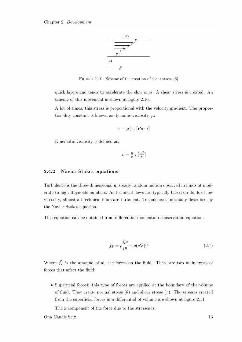
• Viscosity: if a fluid flows in x direction orderly, layered and increasing the velocity

in z direction, a change of the momentum between the layers tends to stop the

Ona Canals Seix 12


Figure 2.10: Scheme of the creation of shear stress [6]

quick layers and tends to accelerate the slow ones. A shear stress is created. An

scheme of this movement is shown at figure 2.10.

A lot of times, this stress is proportional with the velocity gradient. The propor-

tionality constant is known as dynamic viscosity, µ:

τ = µuz ; [Pa · s]

Kinematic viscosity is defined as:

ν = µρ ; [m

2

s ]

2.4.2 Navier-Stokes equations

Turbulence is the three-dimensional unsteady random motion observed in fluids at mod-

erate to high Reynolds numbers. As technical flows are typically based on fluids of low

viscosity, almost all technical flows are turbulent. Turbulence is normally described by

the Navier-Stokes equation.

This equation can be obtained from differential momentum conservation equation.

~fT = ρ∂~v

∂t+ ρ(~v~∇)~v (2.1)

Where ~fT is the amound of all the forces on the fluid. There are two main types of

forces that affect the fluid:

• Superficial forces: this type of forces are applied at the boundary of the volume

of fluid. They create normal stress (θ) and shear stress (τ). The stresses created

from the superficial forces in a differential of volume are shown at figure 2.11.

The x component of the force due to the stresses is:

Ona Canals Seix 13


Figure 2.11: Stress at a differential of volume of fluid created by superficial forces [7]

dFx = ∂θx∂x dxdydz +

∂τyx∂x dxdydz +

∂τzydz dxdydz

The other components of the force follow the same structure. Now, it is possible

to compute the force per unit of volume:

~f = d~FdV = (∂θx∂x +

∂τyx∂y + ∂τzx

∂z )~i+ (∂τxy∂x +

∂θy∂y +

∂τzy∂z )~j + (∂τzz∂x +

∂τyz∂y + ∂θz

∂z )~k

The previous equation can be abbreviated as:

~fS = ~∇~~τ

Where ~~τ is the stress tensor:

~~τ =

θx τxy τxz

τyx θy τyz

τzx τzy θz

• Body forces: they are produced by force fields (gravitational, electromagnetic. . . ).

The most common body force is the gravitational one, and this is the force that

will be considered in this project:

~fg = ρ~g

To sum up, the amount of the forces on the fluid, ~fT is the addition of gravitational

forces and friction forces:

Ona Canals Seix 14


~fT = ρ~g + ~∇~~τ

Finally, the differential momentum conservation equation 2.1, yelds:

ρ~g + ~∇~~τ = ρ∂~v∂t + ρ(~v~∇)~v

However, the stress tensor could be divided in two components; the isotopic part and

the anisotropic part, respectively:

~~τ = −pI + ~~τ ‘

The last term of this equation, for newtonian flows, is related with the symmetric part

of the velocity divergence, as showed at 2.2.

~~τ ′ = 2µ[~∇~vS − 1

3(~∇~v)I] (2.2)

Substituting in the momentum conservation equation, the Navier-Stokes equation is

obtained [19]:

ρ∂~v∂t + ρ(~v~∇)~v = ρ~g − ~∇p+ ~∇{2µ[~∇~vS − 13(~∇~v)I]}

For a incompressible flow with constant viscosity, Navier-Stokes equation can be simpli-

fied as:

ρ∂~v∂t + ρ(~v~∇)~v = ρ~g − ~∇p+ µ~∇2~v

This equation has four unknown variables; the pressure and the 3 components of the

velocity vector. So, another equation is needed in order to have four equations and four

unknown variables, so that the system can be solved. The used equation is continuity

equation, also known as conservation of mass, which for a single phase problem is:

∂ρ

∂t+∇(ρ~v) = 0 (2.3)

Ona Canals Seix 15


2.4.3 Reynolds number

The measure of the non-linearity of Navier-Stokes equation is given by the Reynolds

number, which is defined as:

Re = ρUDµ = UD

ν

Where ρ is the density [kg/m3], U the characteristic velocity of the flow [m/s], D the

characteristic length of the problem [m], µ the dynamic viscosity of the flow [kg/m·s]and ν the kinematic viscosity of the flow [m2/s].

It is a non-dimensional number that estimates the relative weight between the convective

terms ((~v~∇)~v) and the viscous terms (ν4u) of the Navier-Stokes equations. It is an

indicator of the transition between laminar and turbulent flow, which occurs when Re

reaches a critical value.

Reynolds number is used to compare two different experiments with different charac-

teristic parameters during the numerical simulation of a problem. On the first place,

it is important to validate the results of the simulation in order to verify that all the

parameters of the simulation are correct. The validation is performed by comparing the

numerical results with experimental data. The most significant parameter in this kind

of flow is the Reynolds number, if the Reynolds number is the same both results can be

compared. The experiment was performed in such conditions that the Reynolds number

was 3 · 106. So, the Reynolds number of the simulations needs to be the same. Then

considering that the Reynolds number is Re = ρUDµ = 3 · 106: U=1 m/s, D=1 m, ρ = 1

kg/m3 and µ = 3.333·10−7kg/m·s. The values of U, D and ρ are 1 for simplicity reasons

and the dynamic viscosity is then fixed. Even though those values do not correspond to

real values of air properties they are correct given that the important parameter is the

Reynolds number as said before.

2.4.4 RANS models

While turbulence is, in principle, described by the Navier-Stokes equations, it is not fea-

sible in most situations to resolve the wide range of scales in time and space by Direct

Numerical Simulation (DNS) as the CPU requirements would by far exceed the available

computing power for any foreseeable future. For this reason, averaging procedures have

to be applied to the Navier-Stokes equations to filter out all, or at least, parts of the

turbulent spectrum. The most widely applied averaging procedure is Reynolds- aver-

aging (which, for all practical purposes is time-averaging) of the equations, resulting in

Ona Canals Seix 16


the Reynolds- Averaged Navier-Stokes (RANS) equations. By this process, all turbulent

structures are eliminated from the flow and a smooth variation of the averaged velocity

and pressure fields can be obtained.

The fundamental idea is that each magnitude is divided in mean magnitude and fluctu-

ations of the magnitude, for a magnitude φ: φ = φ+ φ′.

Using this fundamental idea at Navier-Stokes equations the new averaged equation is

(for simplicity purposes only x component is showed) [8]:

ρ[∂vx∂t +vx∂vx∂x +vy

∂vx∂y +vz

∂vx∂z ] = − ∂p

∂x+ ∂∂x(τxx−ρv′xv′x)+ ∂

∂y (τxy−ρv′yv′x)+ ∂∂z (τxz−ρv′zv′x)

The Navier-Stokes equations are the same except for the terms −ρv′iv′j . This terms

are responsible for the dissipation caused by fluctuations and form the turbulent stress

tensor or Reynolds tensor:

τ tij = −ρv′iv′j

The value of this tensor is not known but, Prandtl developed the concept of turbulent

viscosity, µt:

τ tij ≈ µt∂vi∂xj

But µt is still unknown. He also defines this variable with the model known as mixing

length model.

µt ≈ ρl2 ∂vi∂xj

The mixing length, l, depends on the problem that is being solved.

2.4.5 Turbulence model

Reynolds- Averaged Navier-Stokes (RANS) equations are very useful, eliminating turbu-

lent structures from the flow and obtaining average values of the important parameters

like pressure and velocity. However, the averaging process introduces additional un-

known terms into the transport equations (Reynolds Stresses and Fluxes) that need to

be provided by suitable turbulence models (turbulence closures).

Ona Canals Seix 17


The choice of turbulence model will depend on considerations such as the physics of

the flow, the established practice for a specific class of problem, the level of accuracy

required, the available computational resources, and the amount of time available for

the simulation.

Shear stress transport (SST) k-ω model has been chosen to do the simulation of this

project.

K-ω models are typically better in predicting adverse pressure gradient boundary layer

flows and separation. The drawback of the standard k- ω equation is a relatively strong

sensitivity of the solution depending on the freestream values of k and ω outside the

shear layer.

It is for this reason that a SST k-ω model has been chosen, this model has been designed

to avoid the freestream sensitivity of the standard k-ω model, by combining elements of

the ω-equation and the ε-equation. In addition, the SST model has been calibrated to

accurately compute flow separation from smooth surfaces.

The constants that this model need are k and ω, they are defined as follows:

Turbulent kinetic energy: k = 1.5(UI)2 = 1.5 · 10−6 ; [m2/s2]

Specific dissipation rate: ω = ρ kµ

(µtµ

)−1= 0.45 ; [1/s]

Where, U is the mean flow velocity (1 m/s), I is the turbulence intensity, a reasonable

value of this parameter is 0.1%, considering the problem in study. Focusing on Specific

dissipation rate, ρ is the density on the air (1kg/m3), k is the turbulent kinetic energy

previously calculated, µ is the dynamic viscosity (3.333 · 10−7kg/ms) and the fraction

µt/µ is known as turbulent viscosity ratio and its value could be approximated as 10

[18].

2.4.6 Wall law and turbulent boundary layer

Turbulence problems are very difficult to solve, a case relatively easier is the study of

the turbulence near of the wall. In this area the velocity of the flow tends softly to the

velocity of the solid, it is known as boundary layer. The boundary layer thickness is

defined as the distance from the wall at which the velocity is 0.99U, considering U the

velocity of the flow far from the wall. This distance is defined as δ at figure 2.12.

It is also possible to see in figure 2.12 the tangential stress in the wall (τp). The expression

v+z = F (y+) is known as the wall law, it is defined by two dimensionless groups [8]:

v+z = vx

v∗ ; y+ = ρv∗yµ

Ona Canals Seix 18


Figure 2.12: Scheme of the boundary layer and its important parameters [8]

where, v∗ is known as friction velocity but, even though it has velocity units it is not a

real velocity. It is defined as:

v∗ =√

τpρ

Focusing in the numerical study, y+ is a non-dimensional distance from the wall to

the first mesh node. It is important to ensure that this first node is not outside of the

boundary layer region. If it happens the mesh of our problem do not have enough quality

to compute the boundary layer behaviour, so the results may be incorrect.

y+ can reach different values, and depending on them the numerical simulation will

be done using different methods. These procedures will be explained at section 4.3

Simulation, where all the parameters of the simulation will be determined.

Ona Canals Seix 19

Chapter 3

Original profile and

transformation

3.1 Reference Aerodynamic Profile

The reference profile that has been chosen to do the aerodynamic optimisation is a

representation of the common profiles used at the inner part of the blades. This flatback

profile is used, exactly, at the first 20% of the length of the blade as seen at 2.3 and 2.4

and it has a maximum thickness ratio about 40% (t/c= 0.4).

As have been said before, this project consists on an optimisation that starts from

another study of another project [9]. This project was made for Efrain Sotelo Ferry, at

2014 and the director is the same than in this project. It is for this reason that this

project continues with the previous work but, taking into account another parameters

and trying to improve a little bit more the aerodynamic performance of the profiles

chosen.

The initial common profile, from which starts the optimisation of the first work, belongs

to one of the most famous families of study, Delft University of Technology, its main

characteristics are explained at table 3.1 and an scheme of its shape is shown at figure

3.1.

Airfoil Designer Maximum thickness ratio (t/c)

DU00-W2-401 Delft Univeristy 0.4

Table 3.1: Initial profile’s characteristics.

As a continuation of the aerodynamic optimisation of the previous study [9], this one

has input data that are the final results form the other project.

20

Chapter 3. Original profile and transformation

Figure 3.1: Initial profile used at the inner part of the rotor blade. [9]

Exactly, from the conclusions is extracted that torque-force coefficient has been improved

about 21% transforming the original profile DU00-W2-401 to a flatback profile with a

thickness at the trailing edge of TE=14%. So, the reference profile of this project is

a flatback profile from DU00-W2-401 with a trailing edge thickness of TE=14%. An

example of these reference profile is shown at 3.2.

Figure 3.2: Reference profiles

3.2 Profile Transformations

3.2.1 Changes on the trailing edge opening

The method used to transform the original profile to flatback consists in adding thickness

symmetrically to either sides of the camber line. As has been said before this method is

more useful to compare some profiles and it is also proved that this method has a better

lift enhancement than the cutting off one.

The equation used to transform the profile is the same used at the previous project [9]

in order to continue the same optimisation. This equation satisfies some general rules

that are used to create flatback profiles; the addition of thickness has to be done after

the point of maximum thickness in order to make sure that the thickness ratio does

not change, it is also important to add the thickness symmetrically to achieve that the

Ona Canals Seix 21


camber line does not change and the distribution of thickness should be soft in order to

avoid adverse effects on the boundary layer.

This equation is defined as:

yfb = yor ± TE/1002 a(x)

where:

yfb = y coordinate of flatback profile (non-dimensional)

yor = y coordinate of original profile (non-dimensional)

TE = Trailing edge thickness with respect to the chord (%)

a(x) = Distribution factor (non-dimensional)

The equation that governs the distribution factor is also the same than in the previous

project:

a(x) = A(x−B)n + C

The distribution factor is characterised by three constants (A, B, and C) that have to be

computed using the boundary conditions, which enable to accomplish the general rules

creating a soft thickness distribution. Other parameters that have to be considered are;

the point where the addition of thickness starts and the thickness at the trailing edge.

Actually, these are the boundary conditions that have to be considered to compute the

constants.

The main difference between the two projects remains in the boundary conditions.

Whereas the soft transition remains constant, the point where the addition of thick-

ness starts is changed. The previous study considered that the point where the addition

of thickness starts was the point of maximum thickness. This study will consider differ-

ent variations of the same profile, by changing the point where the addition of thickness

starts (point ε) and the resulting aerodynamic performances of each case will be com-

pared. This variations are chosen because there is not much information about the

changes that this parameter causes at the aerodynamic performance.

Specifically, four different variations of each profile will be created. The start thickness

point will be located at: the point of maximum thickness, 0.4c, 0.5c and 0.6c.

Considering all the boundary conditions it is possible to write these equations:

Ona Canals Seix 22


x = ε→ a = 0

x = 1→ a = 1

dadx |ε = An(x−B)(n−1) + C = 0

It is also important to define the exponent’s value, n. It has been proved that the value

that produce the softest variation on the thickness is n=0.5 [9].

Finally, the constants are computed as:

A = 1(1−B)n–n(ε−B)n−1

B = ε(1− n)

C = 1−A(1−B)n

To sum up, the value of the constants for each variation on the profile is outlined at table

3.2. A sketch of the 4 variations for the profile is also shown at figure 3.3 (DU00-W2-401).

ε A B C

max.thickness -2.71 0.15 3.4980.4 -4.47 0.20 5.0000.5 -7.46 0.25 7.4600.6 -13.12 0.30 11.978

Table 3.2: Constant values for each variation.

Figure 3.3: Variations of the point of addition of thickness for DU00-W2-401.

Ona Canals Seix 23


3.2.2 Changes on the curvature

The other changes done at the profile are variations on the curvature. This changes have

been done with the aim to improve the aerodynamic performance: it is known that if

the profile has more curvature the lift coefficient increases in general in the linear part.

On the other hand, exists the risk that a high curvature causes an earlier separation

damaging lift and drag curves. So, the changes will increase the positive curvature of

the profile in order to increase the lift coefficient but trying to remain constant the drag

coefficient, obtaining an increase of efficiency and torque coefficient.

The curvature of the initial profile is shown at figure 3.4.a. It can be observed that there

are three different parts; at the front and at the rear part positive curvature whereas

at the middle part negative one. At first, the profile will be transformed to another

one with zero curvature but maintaining the thickness at each point of the chord. This

transformation is shown at figure 3.4.b.

Figure 3.4: Reference profile with a.)initial curvature and with b.) zero curvature.

Exactly, two variations have been done to understand the behaviour of the profile with

different types of curvature and trying to improve the aerodynamic performance of the

initial profile. They are explained below:

• Positive curvature for all the profile: this profiles has a positive curvature with the

point of maximum curvature at 50% of the chord and with a maximum value of

0.02c. At figure 6.7 a superposition between the profile with zero curvature (red)

and the new profile with positive curvature (blue) is shown.

• Accentuation on the positive curvature of the profile: this profile has the same

scheme on the curvature than the reference profile but with a change in the parts of

positive curvature. Exactly, the maximum value of the positive curvature has been

incremented, producing a larger positive curvature. The superposition between the

profile with zero curvature (red) and the profile with accentuated positive curvature

(blue) is shown at figure 6.8.

Ona Canals Seix 24


Figure 3.5: Superposition between zero curvature profile (red) and all positive cur-vature profile (blue)

Figure 3.6: Superposition between zero curvature profile (red) and accentuated pos-itive curvature profile (blue)

Ona Canals Seix 25

Chapter 4

Computational study

4.1 Design

The flatback profile that has been studied in this project is created using the method

of adding thickness to original common profiles. The original common profile used is

DU00-W2-401.

The software that has been chosen to compute the design of the flatback profiles is Excel.

Taking into account that the aeronautic profiles are defined by a set of coordinates, two

different columns have been done: one for the coordinates of the upper surface and

another one for the coordinates of the lower surface.

Then, the transformation of the profile could be done. Actually, the changes done in the

profile are at y coordinates, using the equation with the plus sign, 4.1, in the column of

the upper surface and the equation with the minus sign,4.2, in the column of the lower

surface .

yfb = yor +TE/100

2a(x) (4.1)

yfb = yor − TE/100

2a(x) (4.2)

The values of the constants of the equations depend on the point where starts the

addition of thickness and on the thickness at the trailing edge. They are explained and

computed at section 3.2 Profile transformation.

Finally, the coordinates of the new flatback profiles need to be saved as a Text document,

specifying three columns for the three coordinates that define each point of the profile: x,

26

Chapter 4. Computational study

y and z. In fact, z coordinates will be all zero, taking into account that a 2D configuration

is studied.

4.2 Meshing

The mesh is maybe the most important part of the project. A lot of different parameters

need to be taken into account to have a good mesh like the precision of the results, the

computing power available, the areas of the design that need more precision, etc.

At first, it is important to know what a mesh is, in order to know its most important

parameters. The computational fluid dynamics is based on distretization of the physical

domain into extremely small volumes where the equations that govern the problem are

locally solved. These small volumes are known as cells and the amount of all of these

cells is the mesh. Knowing that, it is easy to see that the quality of the mesh is directly

related with the result of the problem, so it is very important to have a high quality

mesh in order to get good results.

The properties of each cell are assumed constant inside it. So, it is easy to understand

that the bigger the cell is, the less precision there is. For this reason the high quality

meshes have very small cells. Despite of this fact, it is important to considerate the time

used to do the simulation. If the mesh is very fine, a lot of equations will be solved and

this needs time and has computing costs. So, a balance between the precision and the

time and costs will be done in this project in order to have precision enough but do not

spend too time doing the simulations.

There are three main types of meshes:

• Structured meshes: they have regular cells, there is always the same number of

cells at the vertexes and each cell has a fix number of sides.

• Unstructured meshes: they are connected arbitrarily, the cells do not have the

same number of sides. This requires an additional storage cost, considering that

the programme needs to know the configuration of each cell during all the process.

• Hybrid meshes: they are the combination of the two previous types.

A hybrid mesh will be used in this project because the unstructured mesh fits better

with the angulate zone of the trailing edge of the profile and the structured mesh is

useful at the boundary layer.

The programme used to do the mesh is Meshing, from ANSYS.

Ona Canals Seix 27


At first, the area around the profile will be divided in different zones in order to define

the different types of mesh and its quality. Then, the characteristics of each region

will be defined and the mesh will be created. It is important to prove that this mesh

accomplishes all the requirements and fits with the profile. Finally, the zones where

the boundary conditions will be introduced have to be defined. All this procedure is

explained in more detail in the following sections.

4.2.1 Zones division

The area around the profile is divided into 15 different zones in order to define in more

detail the parameters of the mesh, especially at the sensible zones around the profile,

like the boundary layer of the turbulent wake. A scheme of these zones is shown at

figure 4.1.

Figure 4.1: Zones distribution around the profile

There are six regions around the profile located at the part of the boundary layer. In

fact, these regions need to be larger than the real boundary layer in order to let its

expansion without any restriction. Three more zones can be observed after the trailing

edge of the profile, they are located at the turbulent wake.

These nine areas are maybe the most interesting ones due to the fact that these are the

zones where the profile in study interacts with the fluid around it. For this reason, it is

very important to create a mesh with a high density in these zones, in order to be able

to compute the boundary layer’s behaviour and the turbulences created at the wake.

However, the computational domain is about 120 times the chord length of the profile

(L=1m). At the real world the domain around the profile is the atmosphere, but shape

and size need to be determined in order to simulate the profile using CFD. In this study,

Ona Canals Seix 28


the shape chosen is a circumference because it is used to study the profiles fitting well

with them, and the size is 120m to ensure BL is not affected by farfield.

Another circumference is created at the surface. This circumference has 6m of diameter

and defines the unstructured zone of the mesh. This zone extends from the boundary

layer to 3m of radius around the profile in order to avoid obliquity problems in the mesh.

4.2.2 Final mesh

As mentioned above, Meshing has been the software used for the mesh design. This

programme allows defining the parameters of the mesh at each region.

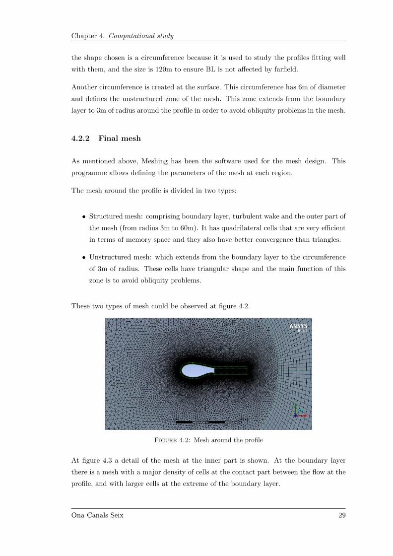
The mesh around the profile is divided in two types:

• Structured mesh: comprising boundary layer, turbulent wake and the outer part of

the mesh (from radius 3m to 60m). It has quadrilateral cells that are very efficient

in terms of memory space and they also have better convergence than triangles.

• Unstructured mesh: which extends from the boundary layer to the circumference

of 3m of radius. These cells have triangular shape and the main function of this

zone is to avoid obliquity problems.

These two types of mesh could be observed at figure 4.2.

Figure 4.2: Mesh around the profile

At figure 4.3 a detail of the mesh at the inner part is shown. At the boundary layer

there is a mesh with a major density of cells at the contact part between the flow at the

profile, and with larger cells at the extreme of the boundary layer.

Ona Canals Seix 29


A structured mesh is recommended in the perpendicular direction of the profile’s perime-

ter [18]. It is needed that the mesh extends always all around the boundary layer. More-

over, more than 15 cells need to be inside the boundary layer in order to guarantee better

results with the advanced models of turbulence like k-ω SST than with other common

methods. A brief explanation of this methods will be done at section 4.3 Simulation.

Figure 4.3: Trailing edge and boundary layer detail.

The mesh is divided in 1500 edges all over the tangential direction of the profile, 750

divisions for the upper surface and 750 more for the lower surface. Focusing of the radial

direction, the boundary layer has 50 divisions with smaller cells at the inner part and

larger ones at the outer part. This principle is also applied at the turbulent wake, having

smaller cells at the zone behind the trailing edge and a growth to the extremes.

Finally, figure 4.4 shows a total view of the mesh done.

Figure 4.4: Total circular mesh of the profile

The final mesh has approximately 420000 cells, with small variations depending on each

profile. In this project the study of the sensibility of the mesh have not been done,

but considering that the mesh is created with the same parameters than the previous

Ona Canals Seix 30


project [9], the same study of sensibility can be used. In the thesis by Sotelo [9] the

number of cells of the mesh chosen at the study of sensibility is lower than the cells of

this project. It is for this reason that can be affirmed that the mesh is good enough

to give good results. However, this mesh could be improved reducing a little bit the

number of cells,in order to reduce the computing cost.

4.2.2.1 Important parameters of the mesh

The quality of the mesh plays a significant role in the accuracy and stability of the

numerical computation, it is for this reason that some indicators are needed to check

the quality of the mesh used.

One of the most important indicators that ANSYS Fluent allows to check is the or-

thogonal quality. This parameter measures the distortion of the cell, in other words, it

considers if the cells have orthogonal angles or not. Therefore, the worst cells will have

an orthogonal quality closer to 0 and the best cells will have an orthogonal quality closer

to 1. The minimum orthogonal quality for all types of cells should be more than 0.01,

with and average value that is significantly higher [18]. This parameter reaches a value

about 0.19 at the meshes used.

Another important indicator is the aspect ratio. It is a measure of the stretching of a

cell. Generally, it is best to avoid sudden and large changes in cell aspect ratios in areas

where the flow field exhibit large changes or strong gradients. This indicator must be

less than 100, considering that the program warns you if this happens. The aspect ratio

of the meshes used is about 24.03, this value is very far from the limit of 100.

It is also important to consider the skewness inside the cell quality. This parameter is

defined as the difference between the shape of the cell and the shape of an equilateral

cell of equivalent volume. Highly skewed cells can decrease accuracy and destabilize

the solution. A general rule is that the maximum skewness for a triangular/tetrahedral

mesh (which is the case of the mesh of this project) should be kept below 0.95, with an

average value that is significantly lower [18].

4.2.3 Zones to determine the boundary conditions

It is important to define different parts of the geometry for the boundary conditions

that must be set later, in Fluent.

The external edges of the regions around the profile are used to define the boundary

conditions. These edges create a circumference with a 120 chords of diameter. Exactly,

Ona Canals Seix 31


the external part of the biggest circle is divided in two parts: the inlet zone is defined

as a half of the circumference and a little bit more and the rest of the circumference is

defined as the outlet area.

It is also needed to define the edge of the profile because is the part where the fluid

interacts with the solid. A scheme of these parts is shown at figure 4.5.

Figure 4.5: Zones where the boundary conditions are defined

4.3 Simulation

The numerical simulation has been performed with ANSYS Fluent software. This pro-

gram computes the flow properties by solving a set of equations on each mesh node. The

equations solved by Fluent are conservation of mass (2.3) and momentum conservation

(2.1) while energy equation is not used in this study because it computes parameters

that are not relevant. Transport equations are also used for a turbulent flow.

As in the previous project [9], this study is bidimensional (planar). There are two main

types of numerical solver; pressure-based and density-based. Density-based solver uses

the continuity equation to obtain the density and the equation of state to obtain the

pressure field. In contrast, pressure-based compute the pressure field using pressure

equation or a combination of continuity and momentum equations. The chosen solver

is Pressure-Based, given that this solver is conceived for low-speed incompressible flows,

and this is the behavior of wind turbines.

Apart from that, time dependence of the problem must be considered. The Reynolds

that characterise the problem is 3 ·106, for this reason it could be considered a turbulent

problem. At first, a steady state study was considered. However, another method had

Ona Canals Seix 32


been used regarding the slow convergence rate obtained due to the fact that a steady

state study is not the best method to solve a turbulent problem. The first step is solving

the problem using steady state study. If it converges the solution is computed, if the

residuals keep oscillating without converge an unsteady study is started. The initial

values of the unsteady study are obtained from the steady state, this fact lets obtain

the solution more quickly and taking advantage of the results computed at the previous

state.

In the unsteady simulation the variables change over time. The time is discretized into

time steps, and the solutions of the equations are computed for each time step. It is

important to set a correct order of magnitude of the time step for the simulation in order

to get good convergence rates.

The indicators of the convergence are the residuals; the problem is converged when they

are smaller than a value defined by the user. After an iteration of the numerical process

the difference of the values of the equations is compared between the result found and

the previous result. This difference is called residual and it is what has to be smaller

than a fixed value in order to make sure that the solution is correct.

The turbulence model that fits better with the simulations of the project is SST K-

ω because it is good predicting adverse pressure gradient boundary layers flows and

separation and the solution is not sensible at free stream values. The fluid around

the profiles is air, which has constant properties that depend on Reynolds number. The

Reynolds number must be the same than in the experimental study (Re =3·106) in order

to characterize the real conditions, so fixing chord (c = 1m), density (ρ = 1Kg/m3) and

flow velocity (U = 1 m/s) the dynamic viscosity is computed as µ = ρUcRe = 3, 333 · 10−7

kg/m ·s .

Two different procedures can be followed depending on the value of the y+. If y+ is

approximately 1, low Reynolds corrections must be selected in the section of the viscous

turbulent model whereas wall functions are not used. However, if the value of y+ is near

to 50 wall functions must be used instead of low Reynolds corrections. In this project,

y+ is of the order of 1, slightly changing depending on the mesh. So, low Reynolds

corrections are selected.

To characterize the problem, the boundary conditions must be fixed. The airfoil is

defined as a viscous wall, choosing the condition no slip. The inlet surface is defined

using the velocity of the flow, which has a module of 1m/s and the direction changes

depending on the angle of attack. The outlet surface is defined with the pressure. This

surface is located at a distance of 60 times the chord of the profile, for this reason it is

assumed that the pressure at this area is not affected by the profile, so it is the ambient

Ona Canals Seix 33


pressure. In this step the characteristic constants of the model of turbulence are defined.

Their values are computed at section 2.4.5 Turbulence model.

The method used to find the solution is Coupled. This coupled algorithm solves the

momentum and pressure-based continuity equations together. The coupled scheme uses

a robust and single phase implementation for steady-state flows, with better performance

than the segregated solution schemes. The steps of this algorithm are illustrated at figure

4.6. It is also important to activate High Order Term Relaxation, this option improves

the stability and the convergence of the solution.

Figure 4.6: Scheme of the pressure-based coupled algorithm [10]

The main parameters of the simulation are summarized at table 4.1.

Solver type Pressure-Based

Time Steady-Transient

Dimension 2D

Turbulence model Viscous SST k-ωTurbulence Kinetic Energy (k) 1.5 10−8 m2/s2

Specific Dissipation Rate (ω) 0.000224 1/s

Material AirDensity (ρ) 1 kg/m3

Dynamic viscosity 3.333 10−7 kg/ms

Boundary conditionsAirfoil Wall No slipInlet Velocity-Inlet (Flow velocity) 1 m/sOutlet Pressure-Outlet (gaurage Pressure) 0 Pa

Solution MethodScheme CoupledSpatial Discretisation First Order Upwind

Monitors Residuals 0.0001

Time StepSize 0.01 sMax itarations/time step 20

Table 4.1: Main parameters of the simulation.

Ona Canals Seix 34

Chapter 5

Profiles validation

At this point, the mesh is done and the parameters that characterize the fluid and the

method of resolution are defined at Fluent ANSYS. Now, it is important to verify that

the hypothesis assumed to define Fluent parameters are correct. It is also needed to

make sure that the mesh has reasonable quality; enough quality to compute turbulence

and separation of the boundary layer but, at the same time, considering that the finer

the mesh is, higher is the time needed to perform the numerical analysis. If any of the

previous requirements is not accomplished some parameters need to be changed.

The verification consists in compare the results obtained by means of the simulation with

the values obtained in an experimental study. Exactly, the dates that are compared in

this chapter are the variation of the Cd and Cl respect to the angle of attack, and the

relation between Cl and Cd, also known as polar curve. These dates are used because

they are the known values from the experimental study. In order to be able to compare

both values, experimental and simulated ones, the Reynolds number in both analyses

needs to be the same. The experimental studies were done with a Reynolds number

Re=3 ·106, so this value is imposed at the numerical analysis. Two different profiles will

be validated; NACA0012 and DU00-W2-401.

5.1 Validation of NACA 0012

At first, a thin and well documented profile was proved. The aim of this first validation

is to prove that the mesh has good quality, it is for this reason that a thin profile is

chosen; to make sure that there is no separation of the boundary layer for small angles

of attack, thus avoid the problems caused by this turbulent flow. The profile validated

is NACA0012, which is shown at figure 5.1.

35

Chapter 5. Profiles validation

Figure 5.1: Draft of the thin profile validated. NACA0012

This is a very common profile, there are a lot of studies and documents about it and this

is a good point because there are a lot of resources where the results can be validated.

Moreover this profile is a good choice because it is symmetric, so the Cl must be zero

for an angle of attack α = 0rad. The comparison between the experimental values and

the results of the simulation is shown at figures 5.2 and 5.3.

Figure 5.2: Comparison between experimental values and simulation results, for aNACA0012 profile. Cl vs. angle of attack

Figure 5.2 shows the relation between Cl and the angle of attack of the profile. The

numerical analysis has provided similar results to the experimental values. However, the

slope of the simulation is slightly lower. Despite this difference, it is so small that the

results can be considered correct.

Figure 5.3: Comparison between experimental values and simulation results, for aNACA0012 profile. Polar curve

Ona Canals Seix 36


As for the polar curve, an important difference can be observed. The simulation results

are higher than the experimental values and in this case this difference cannot be ne-

glected. This difference is caused by the hypothesis assumed in the Fluent parameters.

In the experimental analysis the flow is laminar during most part of the profile, while in

Fluent a turbulent boundary layer is considered for the whole length of the profile. This

are the reason that causes the increase of the Cd. It is important to take into account

that the parameters have been chosen to fit with thick profiles, that are the profiles in

study.

5.2 Validation of DU00-W2-401

The other profile validated is DU00-W2-401. It is the initial reference profile, used to

create the flatback profiles. The target of this validation is to prove that the mesh and

the Fluent parameters are also acceptable for thick profiles and that they also enable

the solver to correctly compute turbulence and the separation of the boundary layer. A

draft of the profile shape is shown at figure 5.4.

Figure 5.4: Draft of the thick profile validated. DU00-W2-401

Two different tests have been done to validate the parameters used. The first one is

shown at figures 5.5 and 5.7 with a red curve whereas the second one has blue color.

Focusing on the relation between Cl and angle of attack, figure 5.5, Cl of the first

test is very similar in the two first points of the graphic, 0 and 5 degrees, creating an

almost horizontal line between both points. From the second point the graphic has a

good behaviour, with a slope similar to the experimental one. However, all the curve is

moved to the right with respect to the experimental curve.

The slope of the second test is almost constant and with the same tendency than the

experimental curve. Up to ten degrees the points are aligned but the curve is also moved

Ona Canals Seix 37


Figure 5.5: Comparison between experimental values and simulation results, for aDU00-W2-401. Cl vs. angle of attack

to the right. However, the difference with respect to the experimental data is not as big

as in the first test.

This difference in the lineal zone could be caused by the separation that appears at the

lower surface for small angles of attack. The profile DU00-W2-401 was created to be

used in wind turbines that operate with angles of attack between 8 and 16 degrees. It is

for this reason that the profile has good efficiency at high angles of attack and that the

flow is separated at low angles. This separation causes poor precision at the lineal zone.

Figure 5.6 shows the velocity distribution around the profile. A blue zone can be observed

at the lower surface of the profile, this zone is the separated one.

Figure 5.6: Draft of the velocity distribution around the profile for an angle of attackof 0 degrees.

The validation of the Cd with respect the angle of attack has better results than the

graphic that relates Cl with angle of attack. For the first test the Cd at 20o do not reach

the experimental value, having a maximum value of 0,17 whereas the experimental one

is 0,27. This big difference evidence that a change on the properties or in the mesh was

needed.

Ona Canals Seix 38


Figure 5.7: Comparison between experimental values and simulation results, for aDU00-W2-401. Cd vs. angle of attack

The changes done between test one and two are the follows:

• Reduction on the size of the cells near the profile, reducing the value of y+ to a

value near to 1.

• Selection of Low Re corrections at viscous turbulent model.

• Change on the computation of the specific dissipation rate, changing it to ω= 0.45

(This change can be done because the turbulent viscosity ratio varies between 1

and 10, this values depends on the problem solved).

The simulations for all the flatback profiles are performed using the second test configu-

ration, so all the procedure explained during the project is referred to the configuration

of the parameters of the second test.

Ona Canals Seix 39

Chapter 6

Results

In this section the results of the numerical simulation are presented. At first, a brief

review of the used profiles is done. Then, the results are schemed using graphs and

tables.

6.1 Study of the changes at the point where the addition

of thickness starts

6.1.1 Geometry

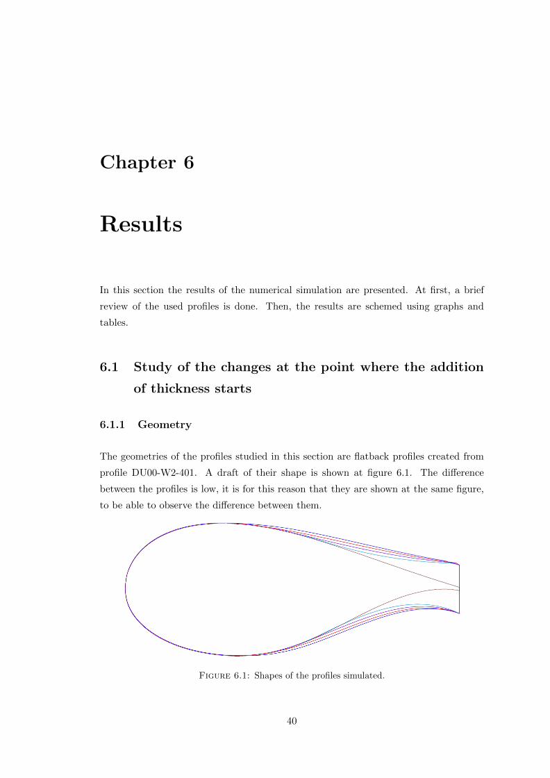
The geometries of the profiles studied in this section are flatback profiles created from

profile DU00-W2-401. A draft of their shape is shown at figure 6.1. The difference

between the profiles is low, it is for this reason that they are shown at the same figure,

to be able to observe the difference between them.

Figure 6.1: Shapes of the profiles simulated.

40

Chapter 6. Results

The parameter that changes between the profiles is the point where the addition of

thickness that creates the flatback profile starts. For simplicity and clarity purposes,

each profile is called as follows and has a characteristic colour:

• Closed: reference profile DU00-W2-401. Before to create the flatback profile and

studied using Fluent. Colour: grey

• Experimental: reference profile DU00-W2-401. Before to create the flatback profile

and experimentally studied. Colour: green

• MAX: profile where the addition of thickness starts at the point of maximum

thickness (approximately at 30% of the chord). Colour: blue

• 0.4c: profile where the addition of thickness starts at the 40% of the chord. Colour:

red


purple


light blue

6.1.2 Results

For wind turbine applications, there are important parameters to consider when com-

paring the performance of different profiles. The most important one is the coefficient

of torque, that produces the movement of the blade, it is also important the efficiency

of the profile that relates lift and drag coefficients. They are also important in order to

see the behaviour of the different profiles. Exactly, a high value on the lift coefficient

is really important at the root zone, where flatback profiles are used, in order to create

a high torque without any penalisation at the bending moment generated at the inner

part of the blade. Comparing the results of flatback profiles with the numerical and

experimental values of the closed profile, different behaviours can be observed.

Starting with the relation between lift coefficient and angle of attack, figure 6.2. Flatback

profiles have higher values of Cl during all the performance. The maximum value of the

Cl is reached later than for the experimental closed profile; this last profile reaches the

maximum Cl at about 8 degrees while the flatback profiles have the maximum later,

at about 15 degrees. This behaviour could be caused by the software, considering that

the simulated closed profile also has a higher stall angle of attack than the experimental

closed profile.

Ona Canals Seix 41

Chapter 6. Results

Figure 6.2: Comparison between experimental values and simulation results, for aDU00-W2-401. Cl vs. angle of attack.

It is important to notice also that for the experimental closed profile, the Cl remains

almost constant from 10 to 20 degrees whereas for flatback profiles, the Cl increases to

the maximum value and then decreases. The maximum Cl for flatback profiles is reached

at 15 degrees and has a value about two times higher than the closed profile.


Focusing on the relation between drag coefficient and angle of attack, figure 6.3, the

tendency of all the profiles is very similar, having an almost horizontal part from 0 to 10

degrees and a growth from 10 to 20 degrees. It is important to pay attention that there

Ona Canals Seix 42

Chapter 6. Results

is not a relevant change between the behaviour of closed profiles and flatback profiles,

in terms of Cd. Despite of this similitude, there are two main differences: the maximum

Cd is higher for flatback profiles than for the simulated closed profile and the Cd0 of the

simulated profiles is higher than for the experimental one. This increase on the Cd for

zero angle of attack could be caused by the fact that the program considers that there

is turbulence at all the profile whereas, in reality, the flow remains attached at the first

part of the profile.

This increase on the Cd for flatback profiles is an expected change. Flatback’s geometry,

with the open trailing edge, creates the separation of the boundary layer and a turbulent

wake behind the profile. Exactly, the open trailing edge produce a very low pressure

behind the profile and for this reason a high pressure drag is created.

The efficiency is an important parameter that characterise the profiles, it is defined as

the division between lift coefficient and drag coefficient and it determines the quality of

the profile. The higher is the efficiency, the better is the profile. The relation between

the efficiency and the angle of attack is shown at figures 6.4 and 6.5.

Figure 6.4: Comparison between experimental values and simulation results, forclosed DU00-W2-401. E vs. angle of attack

Focusing on the experimental results for the closed profile (Experimental) the maximum

efficiency is reached at about 5 degrees with a value of 54. The numerical results of the

simulation for the closed profile (Closed) have the same behaviour, having its maximum

at 5 degrees, but the value of the maximum efficiency is quite small, approximately a

half of the experimental efficiency. The comparison between the results from the closed

profile is shown at figure 6.4.

Ona Canals Seix 43

Chapter 6. Results

Comparing flatback profiles with closed profile, flatback profiles have more efficiency

than the closed profile using numerical simulation, but less than the experimental closed

profile. The point where the maximum efficiency is reached also changes for each flatback

profile. The closed profile has its maximum efficiency at 5 degrees because in this profile

the separation of the boundary layer starts for an angle of attack about 8 degrees, so

form this angle a high increase on the drag coefficient will appear and a high decrease

of the efficiency is produced, as could be observed at figure 6.5.

Figure 6.5: Comparison between experimental values and simulation results, for aDU00-W2-401. E vs. angle of attack

However, the behaviour of the efficiency changes for the flatback profiles, this change

could rely on the changes on the geometry. Flatback profiles are created from closed

profiles, adding thickness symmetrically at both sides of the profile. This increment of

thickness generates a profile with less slope,it is for this reason that the boundary layer

remains attached to the profile longer, delaying the creation of pressure drag caused by

the separation of the boundary layer and producing the increment of drag later. Then,

the efficiency increases during more angles of attack without separation, delaying the

point of maximum efficiency. This delay on the efficiency is good considering that the

range of operation of the wind turbine profiles is about 8 to 16 degrees of angle of attack

[5]. So, the point of maximum efficiency is located at this range for flatback profiles and

improve the performance of the profile.

Actually, the most important parameter that measures the effectiveness of the blade of

wind turbines is Cq, which is a non-dimensional parameter that measures the force done

in the direction of the rotating plane. This force is defined at section 2.2.1 Wind turbine

operation and it depends on two angles, the angle of attack and the twist angle and on

Ona Canals Seix 44

Chapter 6. Results

two coefficients; Cl and Cd. The simulation has been done changing the angle of attack,

so for simplicity reasons twist angle will be considered constant.

Typical twist angles for the 15%–30% radial stations range from roughly 10 to 20 degrees

[5], so the twist angle used in this project is the mean value β= 15 degrees. Then, the

torque coefficient can be computed as:

Cq = Clsin(15 + α)–Cdcos(15 + α)

The torque coefficient values obtained for all the angles of attack and for all the profiles

are showed at table 6.1. They are also schemed at figure 6.6.

Angle of attackCq

Closed MAX 0.4c 0.5c 0.6c

0 -0.008 0.034 0.009 -0.015 -0.010

5 0,115 0.329 0.227 0.301 0.218

10 0,185 0.665 0.340 0.430 0.387

15 0.157 0.809 0.477 0.324 0.276

20 0.099 0.450 0.142 0.066 -0.039

Table 6.1: Torque coefficient for all the profiles depending of the angle of attack.

Figure 6.6: Comparison between experimental values and simulation results, for aDU00-W2-401. delta Cq vs. angle of attack

The maximum torque coefficient is located at 15 degrees of angle of attack for most of

the profiles. It can also be observed at figure 6.6 that the highest Cq is obtained for the

profile that starts the addition of thickness at the point of maximum thickness (MAX).

Actually, it is really interesting to observe that at Cl vs. angle of attack graphic there

is no clear tendency depending on the point where the addition of thickness starts on

Ona Canals Seix 45

Chapter 6. Results

flatback profiles. This means that moving this point forward does not imply that the

Cl is increased or decreased and the same for moving it backwards. It seems to change

randomly for each profile, and the same happens for drag coefficient. However, Cq

indeed shows a decreasing tendency as the point is moved aft of the profile. In fact, the

maximum Cq is obtained by the MAX profile and it decreases for 0.4c, 0.5c and it is

minimum at 0.6c.

6.2 Study of the changes on the curvature of the profile

6.2.1 Geometry

The reference profile of this section is the profile that gives best aerodynamic perfor-

mance at the previous section; flatback profile where the addition of thickness starts at

the point of maximum thickness (approximately at 30% of the chord).

The variations done in this section consist in change the curvature of the profile; in-

creasing the positive curvature in order to increase the Cl0, but maintaining constant

the thickness at each point of the chord. Exactly, this changes consist in a positive

curvature all over the chord and an increment of the positive curvature of the reference

profile, they are better explained at section 3.2 Profile Transformations. A draft of this

variations respect to the profiles with zero curvature are shown at figures 6.7 and 6.8.

Figure 6.7: Superposition between zero curvature profile (red) and all positive cur-vature profile (blue)

Figure 6.8: Superposition between zero curvature profile (red) and accentuated pos-itive curvature profile (blue)

Ona Canals Seix 46

Chapter 6. Results

6.2.2 Results

The aim of this variations is to improve lift performance with a minimum drag penal-

ization, in order to improve the torque coefficient and consequently improve the perfor-

mance of the blade of the wind turbine. It is known that the lift coefficient for an angle

of attack of zero degrees increases when the curvature become more positive. So, the

Cl0 should increase for the two variations of the profile. Table 6.2 shows the values of

the Cl0 for the initial profile (MAX) and for the two variations.

Profile MAX All positive Accent. positive

Cl0 0.306 0.359 0.345

Table 6.2: Comparation of lift coefficients at zero degrees of angle of attack.

The maximum value of Cl0 is reached for the profile that has all the curvature positive

whereas the initial profile (MAX) has the minimum value. These results are consistent

with the predictions done before; having the maximum Cl0 the profile with more positive

curvature and decreasing the values of the initial lift coefficient as the positive curvature

decreases.

Figure 6.9: Comparison between experimental values and simulation results, for aDU00-W2-401. Cl vs. angle of attack.

Considering the lift coefficient for all the angles of attack, it can be observed at figure

6.9 that this behaviour does not remain during all the performance. Despite of the

fact that the Cl0 is increased, the increase on the positive curvature creates a higher

adverse pressure gradient, that promotes an earlier separation of the boundary layer.

So, a decrement of the lift coefficient is produced for some angles of attack.

Focusing on drag coefficient, it can be observed at figure 6.10 that the Cd is higher at

almost all angles of attack. It is important to pay attention on the range of operative

angles of attack, where the drag coefficient for the two variations studied is higher than

the Cd of the MAX flatback profile. This increment on the drag is caused by the fact

Ona Canals Seix 47

Chapter 6. Results

that if the separation of the boundary layer is produced before, the point where the

pressure drag importantly increase is also advanced, creating a higher drag in this zone.


A comparison between velocity fields at 15 degrees for MAX and ”All positive” profiles

is shown at 6.11, it can be observed that the profile with more curvature has separation

of the boundary layer at the upper surface whereas the initial profile, without changes

on the curvature, does not have appreciable separation. These velocity fields agree with

the expected behaviour of the different profiles.

Figure 6.11: Comparison between velocity fields of a.) profile with all the curvaturepositive and b.) MAX profile

Ona Canals Seix 48

Chapter 6. Results

The efficiency for the three profiles is very similar, having its maximum efficiency around

10 degrees, angle compressed in the range of operative angles of attack. The maximum

efficiency is located at this zone because at this angle of attack lift and drag coefficients

are not penalized in a noticeable way by the separation of the boundary layer. The

best efficiency is reached by the MAX profile although the profile with all the curvature

positive has a very similar efficiency. The performance of the different efficiencies is

showed at figure 6.12. While studying the behaviour of the efficiency, the parameter

maximum lift coefficient, Clmax, is more important at the root of the blade considering

that it is directly related with the torque coefficient.

Figure 6.12: Comparison between experimental values and simulation results, for aDU00-W2-401. E vs. angle of attack

Finally, the most important parameter for blades of wind turbines, the torque coefficient

is shown at figure 6.13. It can be observed that the two proposed variations produce

more torque than the reference MAX profile. Despite of the fact that the behaviour

of the three profiles is the same, reaching its maximum value at 15 degrees of angle

of attack, the maximum value for the profile with all the curvature positive is 1.04

whereas the maximum values for the other two profiles are around 0.8. It is interesting

to observe that the increase of Cq is lower for the profile where the positive curvature is

accentuated than for the profile with all the curvature positive. This behaviour shows

that the changes on the curvature are very important because the curvature is directly

related with the lift coefficient.

The computation of the increment of Cq at 15 degrees of angle of attack of the profiles

that reaches better performance, profile with all the curvature positive, with respect to

the reference profile, MAX, is shown at table 6.3. It can be observed that the maximum

increment that produces the variation on the curvature of the profile is about 30%.

Ona Canals Seix 49

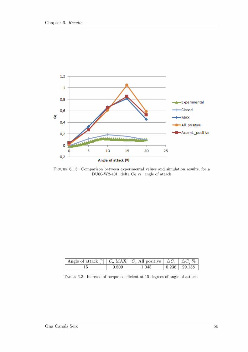
Chapter 6. Results

Figure 6.13: Comparison between experimental values and simulation results, for aDU00-W2-401. delta Cq vs. angle of attack

Angle of attack [o] Cq MAX Cq All positive 4Cq 4Cq %

15 0.809 1.045 0.236 29.138

Table 6.3: Increase of torque coefficient at 15 degrees of angle of attack.

Ona Canals Seix 50

Chapter 7

Budget

The budget of this project considers the main expenses effectuated during all the process,

including numerical calculations and writing of the study. Considering that this project

consist basically in a numerical simulation that is effectuated with a computer, there are

not expenses for material. The two main expenses of the project are human resources

and computational resources.

For human resources it is important to consider the spent hours of work and multiply

them by the cost per hour of an engineer. Considering that this project has been done

in 390 hours and that the cost per hours of an engineer is about 15 e/ hour, the final

cost of human resources is 5850 e.

As have been said before the computational expenses only include the price of the licence

of the software used. In this project the software used is ANSYS Fluent 15.0. A licence

is necessary to use this program, this licence is about 24903.36 e[21]. Considering that

this licence is annually and that this project has been done during 3 month, the cost of

this software for this time is 6225.84 e.

The costs of the project can be computed as the addition between the human resources

time and the computational costs. The final cost of the project appears at the following

table, 7.1.

Cost [e]

Human resources 5850

Computational resources 6225.84

Total 12075.84

Table 7.1: Final cost of the project

51

Chapter 8

Environmental analysis

In this chapter an environmental analysis will be done. There are two main aspects to fo-

cus on: the environmental effect of the elaboration of this project, and the environmental

effect of the implementation of the changes proposed in this study.

On the one hand, the realised study and the comparison of the obtained results do not

have any relevant repercussion on the environment. The only parameter that could be

taken into account is the power consumption produced by the laptop and the computer

used to do the study.

On the other hand, the theme of this project is strongly related with the creation of a

better environment, using renewable resources instead of fossil fuels.

Current electricity generation relies mainly on burning fossil fuels, this procedure gen-

erate carbon dioxide and moreover, waste much of their primary input energy. So,

a complete transformation of the way we produce, consume and distribute energy is

required, while maintaining economic growth.

Wind turbines have a lot of good environmental effects. This technology enables to

reduce consume of fossil fuels, which produce carbon dioxide that generates the climatic

change. Data from the wind industries show that it is possible to maintain a growth

rate of about 30% in the renewable energy sector [17]. As have been said before, wind

turbine generators tend to be larger in order to produce more power. These turbines and

their evolution could create some negative environmental effects like acoustic problems

because the motion of the blades creates noise that could affect the ecosystem of the

wind farm. The birds ecosystem is also affected because they can impact with the blades

of the turbine. Moreover, wind farms create also a visual contamination, considering

their large volume.

52

Chapter 8. Environmental analysis

Focusing on this project, its aim is to improve the aerodynamic performance of the flat-

back profiles, which enables to increase the power generated for the wind turbine. This

optimisation reduces the bad effects of the wind turbine, creating smaller wind farms

with the same power generated. It also helps on the transformation on the production

of the energy, changing fossil fuels for renewable resources.

Ona Canals Seix 53

Chapter 9

Conclusions

9.1 Conclusions

On the one hand, knowledge about numerical analysis and problems resolution by means

of computational fluid dynamics has been acquired. On the other hand, this project has

been useful as a introduction at wind turbines and their blades, specially at the inner

part of the blade.

Nowadays, a lot of studies are focused in designing better thick profiles. This necessity

comes from the fact that at the inner part of the blade, thick profiles are used for

structural purposes and also because they are a transition between the common profiles

of the blade and the cylindrical axis that links blade and gearbox. This type of profiles

have a maximum thickness higher than the 30% of the chord ( tc > 0.3) so, there is a big

slope at the rear part of the profiles, creating a strong pressure gradient which causes

the separation of the boundary layer. This separation creates a dramatic increment on

the drag and a decrement of the lift.

Flatback profiles are a good alternative to design a more energetic root for a wind turbine

blade. They are created adding thickness at the rear part of the thick common profiles

creating a blunt trailing edge. This increment of thickness reduces the slope of the profile,

delaying the separation of the boundary layer and increasing the lift performance of the

profile. It is true that the drag also increase but the growth of lift is higher, so the total

performances of the profile improves.

Focusing on this project, the profiles proved are common DU00-W2-401 closed profile

and flatback profiles created from this closed profile. The change between them is the

point where the addition of thickness starts.

54

Chapter 9. Conclusions

The main changes observed between closed and flatback profiles are the increase of lift

and the increase also of drag. The results of this project, section 6.1.2 Results, show

that an important increase on lift force appears using flatback profiles. This increase

appears for high angles of attack, caused by the delay of the boundary layer separation.

The results of the simulation show that the maximum lift coefficient for flarback profiles

are two times the maximum lift coefficient for the closed profile. The drag coefficient

for flatback profiles also increases with respect to the Cd of the simulated closed profile,

however this increment is smaller than the lift one.

The differences between flatback profiles are not easy to see. On drag vs. angle of attack

graphic it can be observed that as the point where the addition of thickness starts is

moved aft of the profile, the drag coefficient increases. The most important parameter

that must be considered in wind turbine applications is the torque coefficient, Cq, it

represents the amount of force at rotational plane direction. This parameter reaches

its maximum value for flatback MAX (flatback profile where the addition of thickness

starts at the point of maximum thickness). Cq decreases as the point where the addition

of thickness starts is moved aft of he profile. It is for this reason that can be affirmed

that the most aerodynamically optimal profile is the flatback with the start of addition

of thickness at the point of maximum thickness. This result agrees with the results of

similar studies done in parallel of this one.

Considering the changes done on the curvature of the profile, it has been proved that

both, the accentuation of the positive curvature and the change to get a profile with

positive curvature, improve the aerodynamic performance of the profile. Reaching the

best values of torque performance for the profile with positive curvature for all the chord

of the profile. Despite of the fact that more curvature promotes a higher adverse pressure

gradient that produces an earlier separation of the boundary layer and this separation

creates more drag, the increment of lift is higher than the increment of drag, obtaining

higher values of torque coefficient for the profiles with more curvature than for the initial

profile, MAX. Exactly, the maximum increment is reached at angle of attack 15 degrees

for the profile with all the curvature positive, this maximum value is 30% higher than

the torque coefficient for the initial profile. As a result, it can be concluded that the

best studied profile is a flatback profile created from DU00-W2-401 with TE of 14%, the

addition of thickness starts at the point of maximum thickness and all the curvature of

the profile is positive with a maximum of 0.02c at the 50% of the chord. However, this

profile is not optimised with respect to the curvature, only two configurations have been

tried in order to improve its performance.

Finally, it has been proved that the usage of flatback profiles could improve a lot the

performance of the inner part of the blade of wind turbines, incrementing the coefficient

Ona Canals Seix 55

Chapter 9. Conclusions

of torque and lift coefficient all over the work range. So, this type of profiles have a big

potential to improve the wind turbine blades.

9.2 Proposed future work

This project consists in an aerodynamic optimisation of the profiles done in 2D and

using mostly steady computations. Taking into account that the objects in study are

thick profiles, turbulence need to be considered and the best method to compute the

turbulence is by means of a unsteady study in stead of a steady one. Is is also important

to compute the turbulence using a 3D geometry, considering that the turbulence is

a three-dimensional unsteady random motion. This type of studies requires a basic

knowledge about flatback profiles and their aerodynamic behaviour, moreover they are

more computationally expensive. Now, they can be performed considering that there

is a previous background established by this work and by Sotelo [9]. The following list

contains the proposed future work:

• 3D analysis of a segment of the inner part of the blade.

• Unsteady analysis of flatback profiles.

• Unsteady analysis of a 3D segment of the inner part of the blade.

• Analysis of flatback profiles changing parameters that have not been changed yet.

Ona Canals Seix 56

Chapter 10

Planning of the future work

The proposal of future work that is planned in this chapter is the aerodynamic optimi-

sation of the inner part of the blade. In this case the study will be in 3D instead of 2D.

Despite of the addition of one dimension at the problem, the activities that have to be

developed are really similar to the ones done in this project. It is for this reason that

the Gantt diagram and the other elements used for the planning of the study, will be

very similar to the ones that appear in the project charter of this project.

A correct planning of the project is very important in order to achieve its goal using

efficiently the time and the resources. Taking into account that the entire project could

be done by the same person, almost all the activities will done in series except the

writing, which has been done in parallel as the evolution of the other activities.

The body of the project are the simulations of the flatback profiles that are done using

CFD. So, the activities that have been longer are the activities related with the software.

At first a good mesh that fits the geometry needs to be created, and then it is necessary

to know the boundary conditions used to define the problem. It is necessary to spend a

lot of time during the simulations. And the port-process and the analysis of the results

is very important, so it is necessary to do this part step by step and this takes time.

A brief explanation of the main activities of the project is showed:

• Research of information and documentation

– State of the art and information of flatback profiles

To know the evolution of the flatback profiles and understand the necessary to

create this type of profiles in order to do the best optimisation.It is important

also to study the implementation of this profile at the inner part of the blade.

57

Chapter 10. Planning of the future work

– Research of related information

To find important information related with the flatback profiles and wind tur-

bine blades that is necessary for the project.

• Creation of a new geometry

The new geometry of the profile can be created from an original profile and the

optimised profile created in this project. In the 3D project it is also important to

focus on the shape of the whole blade in order to create a geometry that not only

optimises aerodynamically the profile, but optimise aerodynamically the whole blade

of the wind turbine. In order to do this 3D optimisation two main parameters need

to be considered: the chords distribution and the twist angle distribution.

• Software tasks

– Ansys software learning

Learn how to insert a geometry, mesh the geometry and post-process the re-

sults.

– Creation of an appropriate mesh for each geometry

Create a good mesh for each 3D geometry that fits with the different geometries

and gets convergence.

– Simulation of each geometry

Simulate each mesh considering boundary conditions.

– Post-process of the simulation

Extract significant values of the results of the simulation.

• Results evaluation

Ensure that the obtained results are consistent and draw conclusions. In this sec-

tion the geometry that best adapts to the root blade characteristics of a wind turbine

will be found. This characteristics combine high CL and high E. The best geometry

will be that one that gives the highest torque value which is giving the electrical

energy generation.

• Writing of the TFG

Writing of all the deliverables of the TFG; report, annexes and budget.

• Revision

Make sure that the work that has been done is correct.

Ona Canals Seix 58


Code of task Task identificacion Preceding task(s)

SA State of the art -

RI Research information -

NG New Geometry SA, RI

LS Learn Software -

CM Create a mesh LS, NG

S Simulations of each geometry CM

P Post-process S

RE Results evaluation P

W Writing of the TFG -

R Revision RE

Table 10.1: Relationship between activities.

Code of task Task identificacion Time (hours)

SA State of the art 25

RI Research information 25

NG New Geometry 50

LS Learn Software 65

CM Create a mesh 120

S Simulations of each geometry 150

P Post-process 40

RE Results evaluation 40

W Writing of the TFG 85

R Revision 10

Table 10.2: Hours spent for each task.

The following tables show the relation between the activities described before 10.1, and

the spent time for each activity 10.2.

At table 10.2 an important increase of hours of work could be observed comparing with

the spent hours in this project. The reason of this increment lies in the fact that the

study of a 3D geometry is quite more complicated than a 2D study. For instance, the

creation of the new geometry needs to consider the evolution of the flatback profiles

along the blade. So, the interaction between the profiles have to be considered during

the aerodynamic optimisation. The mesh will be also more complicated, having nodes

in three directions. It has to fit not only with one profile, but in a part of the blade.

This 3D mesh has more nodes than a 2D mesh, is for this reason that the simulation of

each geometry will be longer and heavier.

Adding all the hours predicted at table 10.2 the time needed to do this project is about

610 hours. As said before, this is a larger project that can be done in more time or with

the same time but spending more daily hours, considering that is an academic project

it could be a focused on GrEVA.

Ona Canals Seix 59


At last, a possible planning of the main activities could be the Gannt diagram shown

at figure 10.1. Actually, this is the Gantt used in the project charter of this project

but,considering the similarities of the procedure the only change needed is to multiply

per two the hours spent each day.

Figure 10.1: Gantt diagram of the project

Ona Canals Seix 60

Bibliography

[1] D. Laird. Blade Design Codes. Sandia National Laboratories, 2004.

[2] C.P. van Dam. Blade Aerodynamics .

[3] J.A. Paquette and P.S. Veers. Increased strength in wind turbine blades through

innovative structural design. In Sandia National Laboratiories.

[4] Renewable UK. Wind energy, 2015. URL http://www.renewableuk.com/en/

renewable-energy/wind-energy/index.cfm.

[5] K. J. Standish and C. P. van Dam. Aerodynamic Analysis of Blunt Trailing Edge

Airfoils. Journal of Solar Energy Engineering, (4):479. ISSN 01996231. doi: 10.

1115/1.1629103.

[6] Castilla R. and Gamez-Montero P.J. Introduccion. Concepto de fluido y propiedades

basicas, 2011.

[7] Castilla R. and Gamez-Montero P.J. Fuerzas sobre los fluidos, 2011.

[8] Castilla R. and Gamez-Montero P.J. Introduccion a la turbulencia, 2011.

[9] Efrain Sotelo Ferry. Estudio aerodinamico y optimizacion de perfiles flatback apri-

cado a aerogeneradores. Master’s thesis, Universitat politecnica de Catalunya, 2014.

[10] ANSYS Fluent Theory Guide. ANSYS Inc., January 2009.

[11] Tony Burton, David Shapre, Nick Jenkins, and Ervin Bossanyi. Wind Energy

Handbook.

[12] Ozlem Ceyhan. AERODYNAMIC DESIGN AND OPTIMIZATION OF HORI-

ZONTAL AXIS WIND TURBINES BY USING BEM THEORY AND GENETIC

ALGORITM. 2008.

[13] Greenpeace. WIND FORCE 12. (June):52, 2005.

61

http://www.renewableuk.com/en/renewable-energy/wind-energy/index.cfm

http://www.renewableuk.com/en/renewable-energy/wind-energy/index.cfm

Bibliography

[14] Xiaomin Chen and Ramesh Agarwal. Optimization of Flatback Airfoils for Wind-

Turbine Blades Using a Genetic Algorithm. Journal of Aircraft, 49(2):622–629,

March 2012. ISSN 0021-8669. doi: 10.2514/1.C031614. URL http://arc.aiaa.

org/doi/abs/10.2514/1.C031614.

[15] K. J. Jackson, M. D. Zuteck, C. P. van Dam, K. J. Standish, and D. Berry.

Innovative design approaches for large wind turbine blades. Wind Energy, 8

(2):141–171, April 2005. ISSN 1095-4244. doi: 10.1002/we.128. URL http:

//doi.wiley.com/10.1002/we.128.

[16] Xiaomin Chen and Ramesh K. Agarwal. Optimization of Wind Turbine Blade

Airfoils Using a Multi-Objective Genetic Algorithm. Journal of Aircraft, 50(2):

519–527, March 2013. ISSN 0021-8669. doi: 10.2514/1.C031910. URL http:

//arc.aiaa.org/doi/abs/10.2514/1.C031910.

[17] Josche Murth. Energy revolution, July 2012. URL http://www.greenpeace.org/

international/Global/international/publications/climate/2012/Energy%

20Revolution%202012/ER2012.pdf.

[18] ANSYS Fluent User’s Guide. ANSYS Inc., Novembre 2013.

[19] Castilla R. and Gamez-Montero P.J. Las ecuaciones de Navier-Stokes, 2011.

[20] LEAP CFD Team. Turbulence part 2 - wall functions and y+ re-

quirements, 2012. URL http://www.computationalfluiddynamics.com.au/

tips-tricks-turbulence-wall-functions-and-y-requirements/.

[21] ANSYS. Authorized Information Technology Schedule Price List, 2014.

Ona Canals Seix 62

http://arc.aiaa.org/doi/abs/10.2514/1.C031614


http://doi.wiley.com/10.1002/we.128

http://doi.wiley.com/10.1002/we.128



http://www.greenpeace.org/international/Global/international/publications/climate/2012/Energy%20Revolution%202012/ER2012.pdf



http://www.computationalfluiddynamics.com.au/tips-tricks-turbulence-wall-functions-and-y-requirements/

http://www.computationalfluiddynamics.com.au/tips-tricks-turbulence-wall-functions-and-y-requirements/

aerodynamic study on the design and optimization of ... · aerodynamic study on the design and...

Documents