aerodynamic sensitivity analysis of rotor imbalance and...

Aerodynamic Sensitivity Analysis of Rotor Imbalance and Shear Web Disbond Detection Strategies for Offshore

Structural Health Prognostics Management of Wind Turbine Blades

Noah J. Myrent1 and Douglas E. Adams2 Vanderbilt Laboratory for Systems Integrity and Reliability, Nashville, TN, 37226

D. Todd Griffith3 Sandia National Laboratories, Albuquerque, NM, 87185

Operations and maintenance costs for offshore wind plants are projected to be considerably higher than the current costs for land-based wind plants. One way to reduce these costs would be to implement a structural health and prognostic management (SHPM) system as part of a condition based maintenance paradigm with smart load management. To facilitate the development of such a system a multiscale modeling approach has been developed to identify how the underlying physics of the system are affected by the presence of damage and faults, and how these changes manifest themselves in the operational response of a full turbine. This methodology was used to perform a sensitivity analysis, investigating several inflow conditions in an effort to further evaluate the maturity of rotor imbalance and shear web disbond detection strategies developed in past efforts under variable inflow conditions as would be experienced in actual operation. Based on an aerodynamic sensitivity analysis of the model, the operational measurements used for the pilot study in the detection of pitch error, mass imbalance, and shear web disbond were utilized to confirm the validity of the detection strategies for all three damage/fault cases. Detection strategies were refined for these fault mechanisms and probabilities of detection (POD) were calculated. For all three fault mechanisms, the probability of detecting each fault was 96% or higher for the optimized wind speed ranges of the laminar, 30% horizontal shear, and 60% horizontal shear wind profiles. This aerodynamic sensitivity study contributes to the evaluation of structural health monitoring information with the goal to reduce operations and maintenance costs for an offshore wind farm while increasing turbine availability and overall profit.

Nomenclature G = mass imbalance grade Reff = effective span-wise location of the added mass Sk(f) = turbulence model spectra at frequency f for velocity component k Uper = calculated change in blade mass W = rotor mass

1 Staff Engineer, Wind Energy Research Lead, Vanderbilt Laboratory for Systems Integrity & Reliability (LaSIR), [email protected], AIAA Member 2 Distinguished Professor and Chair, Civil & Environmental Engineering, [email protected]. 3 Principal Member of the Technical Staff, Wind and Water Power Technologies, [email protected], AIAA Associate Fellow.

American Institute of Aeronautics and Astronautics

1

Dow

nloa

ded

by S

AN

DIA

NA

TIO

NA

L L

AB

OR

AT

OR

IES

on O

ctob

er 2

2, 2

014

| http

://ar

c.ai

aa.o

rg |

DO

I: 1

0.25

14/6

.201

4-07

14

32nd ASME Wind Energy Symposium

13-17 January 2014, National Harbor, Maryland

AIAA 2014-0714

Copyright © 2014 by the American Institute of Aeronautics and Astronautics, Inc. All rights reserved.

AIAA SciTech

I. Introduction ffshore wind energy in the United States is an untapped energy resource that could play a pivotal role in helping the U.S. obtain an energy portfolio composed of clean, renewable and diversified resources. Some of the

drivers for the utilization of offshore wind include the proximity of the offshore resources to population centers and the potential for higher capacity factors due to higher resource winds1. Because of these drivers and other potential benefits of offshore wind, the Offshore Wind Innovation and Demonstration initiative has developed an ambitious goal of deploying 10 GW of offshore capacity by 2020 with cost of energy reductions. One potential way in which these operations and maintenance (O&M) costs could be addressed is through the use of a structural health and prognostics management (SHPM) system as part of a condition based maintenance (CBM) paradigm4-10. By continuously monitoring the health, or condition, of structural components in each wind turbine, required maintenance actions can be scheduled ahead of time and performed when they are needed rather than on a preset schedule or only after failure has already occurred. The benefits of a CBM strategy are expected to include less regular maintenance, the avoidance or reduction of unscheduled maintenance and improved supply chain management6-9.

In an effort to map out the SHPM problem with application to wind turbine rotor blades and also provide an example case study, an initial roadmap was developed by Sandia National Laboratories for a combining structural health monitoring and prognostics management assets into a SHPM system as documented in References 12 and 25. Past work includes preliminary pilot studies performed on the turbine response effects due to trailing edge disbond and later for rotor imbalance and shear web disbond24,26. As a result of the preliminary studies, detection strategies were constructed for blade pitch error, blade mass imbalance, and blade shear web disbond. The work presented in this paper involves the sensitivity analysis of the preliminary detection strategies in an effort to validate the developed damage detection algorithms and evaluate their success in several different aerodynamic loading cases that are representative of inflow operating conditions. The shear web disbond sensitivity study includes the addition of several disbond lengths as well.

The paper is organized as follows. In Section II, the 5-MW turbine model used in these simulations is presented. In Section III, the initial pilot studies of rotor imbalance and shear web disbond (from References 24 and 26) are reviewed, then in Sections IV and V, results of inflow sensitivity analysis and calculations of probability of detection (POD) values and the effects of inflow variability on POD values are presented for rotor imbalance and shear web disbond, respectively. In Section VI, the major findings of this work are summarized.

II. Five Megawatt Offshore Turbine Model

As part of an ongoing structural health and prognostics management (SHPM) project at Sandia National Laboratories for wind turbines, the simulations in this report were performed using a representative utility-scale wind turbine model. The model, known as the National Renewable Energy Laboratory (NREL) offshore 5-MW baseline wind turbine model, was developed by NREL to support studies aimed at assessing offshore wind technology11. It is a three-bladed, upwind, variable-speed, variable blade-pitch-to-feather-controlled turbine and was created using available design information from documents published by wind turbine manufacturers, with a focus on the REpower 5-MW turbine. Basic specifications of the model configuration are listed in Table 1.

Table 1. Gross Properties of the NREL 5-MW Baseline Wind Turbine11 Property Value

Rating 5MW Rotor Orientation, Configuration Upwind, 3 blades Control Variable Speed, Collective Pitch Drivetrain High Speed, Multiple-Stage Gearbox Rotor, Hub Diameter 126 m, 3 m Hub Height 90 m Cut-in, Rated, Cut-out Wind Speed 3 m/s, 11.4 m/s, 25 m/s Cut-in, Rated Rotor Speed 6.9 rpm, 12.1 rpm Rated Tip Speed 80 m/s Overhang, Shaft Tilt, Precone 5m, 5°, 2.5° Rotor Mass, Nacelle Mass, Tower Mass 110,000 kg; 240,000 kg; 347,460 kg Water Depth 20 m Wave Model JONSWAP/Pierson-Moskowitz Spectrum Significant Wave Height 6 m Platform Fixed-Bottom Monopile

O


2

Dow

nloa

ded

by S

AN

DIA

NA

TIO

NA

L L

AB

OR

AT

OR

IES

on O

ctob

er 2

2, 2

014

| http

://ar

c.ai

aa.o

rg |

DO

I: 1

0.25

14/6

.201

4-07

14

Two-thirds of the blade span utilizes the TU-Delft family of airfoils, while the outboard one-third of the blade span utilizes the NACA 64-series airfoils. Intermediate airfoil shapes were developed that preserve the blending of camber lines as well as a smooth blade thickness profile. Figure 1 shows the finite element model of the blade developed at Sandia12 in ANSYS with the colored sections representing different composite materials. This high degree-of-freedom model was translated into a model consisting of several beam elements using Sandia’s Blade Property Extraction tool (BPE)22. BPE works by applying loads in each of the six degrees of freedom at the tip of the blade model in ANSYS, then processing the resulting displacements at selected nodes along the blade to generate the 6x6 Timoshenko stiffness matrices for the beam discretization. This reduced degree-of-freedom model is subsequently used to define the blade properties used in the turbine aero-elastic simulations (e.g. NREL’s Fatigue, Aerodynamics, Structures and Turbulence (FAST) software13).

Figure 1. ANSYS finite element mesh for the 5-MW blade model12

FAST uses six coordinate systems for input and output parameters13. Note that the FAST User’s Guide coordinate

system images use a downwind turbine configuration; however, the same coordinate systems apply in the case of the upwind turbine being referred to in this work, but the orientation of the x axis changes so that in either configuration it is pointing in the nominally downwind direction. The rotor shaft coordinate system is shown in Figure 2a. This coordinate system does not rotate with the rotor, but it translates and rotates with the tower and yaws with the nacelle. In addition to output variables related to the low speed shaft, the nacelle inertial measurements also use this coordinate system. Some shaft outputs, such as shear force in the low speed shaft, are measured in both a non-rotating coordinate system and a rotating coordinate system; these are differentiated by using an “s” or “a” subscript, respectively. The tower base coordinate system shown in Figure 2b is fixed in the support platform, thus rotating and translating with the platform. The tower-top/base-plate coordinate system shown in Figure 2c is fixed to the top of the tower. It translates and rotates with the motion of the platform and tower top, but it does not yaw with the nacelle.

(a) (b) (c)

Figure2. (a) Shaft Coordinate System13; (b) Tower Base Coordinate System13; (c) Tower-Top/Base-Plate Coordinate System13

III. Rotor Mass/Aerodynamic Imbalance and Shear Web Disbond Preliminary Studies

This section summarizes the past work involving the preliminary characterization studies on rotor imbalance and shear web disbond24. The initial rotor imbalance study includes the Master’s thesis work performed by Kusnick23. Computer simulations were carried out using the 5-MW turbine model described in Section II. Modeling was performed using NREL’s FAST code, which is a comprehensive aeroelastic simulator for two and three-bladed horizontal axis wind turbines (HAWTs). The code provides the means to manipulate a variety of input parameters, including turbine control settings, environmental conditions, blade and tower models, drivetrain and generator parameters, and many others. There are also hundreds of possible outputs, including blade inertial measurements and generator power.


3

Dow

nloa

ded

by S

AN

DIA

NA

TIO

NA

L L

AB

OR

AT

OR

IES

on O

ctob

er 2

2, 2

014

| http

://ar

c.ai

aa.o

rg |

DO

I: 1

0.25

14/6

.201

4-07

14

FAST uses AeroDyn to calculate the aerodynamics of HAWTs. AeroDyn is an aerodynamic simulation code which uses several subroutines for wind turbine applications, including the blade element momentum theory, the generalized dynamic-wake theory, the semi-empirical Beddoes-Leishman dynamic stall model, and a tower shadow model. The FAST model combines a modal and multibody dynamics formulation, and performs a time-marching analysis of the nonlinear equations of motion. For a more detailed description of the working principles of the code, see the FAST User’s Guide13.

A. Rotor Imbalance Pilot Study In the pilot studies24, simulations were carried out in a unidirectional, constant-speed, vertically sheared wind

environment, rather than using the random and turbulent wind input conditions that are also available as inputs in FAST. The wind direction was oriented at 0°, directly perpendicular to the rotor plane, and the yaw degree of freedom was turned off in the FAST input file. The wind speed was set to 11 m/s, with a 1/7 power law vertical shear profile. Setting the wind speed to just below the rated speed of 11.4 m/s ensured that in the case of pitch error of a single blade, the other two blades would always be pitched to zero degrees to maximize the power output of the turbine, thus keeping those variables constant. The sample time spacing was set to 0.01 seconds, corresponding to a sample rate of 100 Hz. Because the per-revolution harmonics were mainly of interest and the maximum rotor speed was 12.1 rpm, or 0.2 Hz, this sample rate was sufficient. Simulations were conducted in three phases: (1) aerodynamic imbalances caused by pitch error, (2) mass imbalances, and (3) simultaneous aerodynamic and mass imbalances. Two hundred output variables were recorded from the simulations, including generator power, low speed shaft torque, tri-axial blade accelerations along the span, nacelle accelerations, and many others for use in the sensitivity of damage/fault studies.

Aerodynamic asymmetry due to pitch error was established directly by the blade pitch angle parameters used in FAST. The turbine control parameters BlPitch(1), BlPitch(2), and BlPitch(3) are the initial pitch angles and BlPitchF(1), BlPitchF(2), and BlPitchF(3) are the final blade pitch angles at the completion of the time marching simulation. As for mass imbalance, the asymmetry was applied by increasing the mass density of blade three at a particular blade span-wise section in the FAST blade input file. The magnitudes of the mass imbalances chosen were based on two references. The first is the acceptable residual imbalance method employed by Pruftechnik Condition Monitoring GmbH, a German company which performs field-balancing of wind turbine rotors14. This company applies a fairly standard field balancing procedure: initial vibration measurements are taken from within the nacelle, a trial mass is added to the rotor and its effects are measured, and the balancing software then determines suggested balancing weights and locations. A detailed explanation of the general rotor balancing procedure and calculations can be found in Bruel & Kjaer’s application notes16. Pruftechnik quantifies the permissible residual imbalance based on the standard DIN ISO1940-1: Mechanical Vibration – Balance Quality Requirements for Rotors in a Constant (Rigid) State – Part 1: Specification and Verification of Balance Tolerances. This standard provides permissible residual imbalance levels in the rotor, with different quality grades, G, depending on the application. The imbalance magnitude is found using the rotor’s operational speed, rotor weight, and the balancing radius, which is the span location of the mass imbalance. Plots in the standard provide the permissible imbalance in gram-mm/kg which are based on the rotor speed and G grade. A second source for determining mass imbalance testing levels was Moog Incorporated’s fiber-optic based rotor monitoring system, which claims imbalance detection down to 0.5% of the total blade mass of all three blades17. For consistency and ease of comparison, it will be assumed that this imbalance is acting at the mass center of a single blade, and it will be translated to an ISO1940-1 G quality grade.

The FAST blade input file for the blade model contains 23 section locations for specifying section properties. However, for computational purposes, the 23 locations are interpolated down to 17 nodes as specified in the AeroDyn input file for application of the aerodynamic forces in FAST. The effective span-wise location of the added mass was computed using a moment balance as follows in equation (1):

1

1

( ) ( )

( ) ( ),

Ni i i

iN

i ii

dm dr r

effdm dr

R =

=

⋅ ⋅

⋅

∑=∑

(1)

where Reff is the effective span-wise location of the added mass, N is the number of blade sections, (dm)i is the change in mass density of blade section i in kg/meter, (dr)i is the length of the ith blade section in meters, and ri is the radial location of the blade section in meters. The mass imbalance level G is defined in Equation (2), shown below. The rotor mass, W, was computed using the newly interpolated blade mass properties in addition to the hub mass. The rotational speed N was found by running the simulations, which was 11.8 rpm regardless of the mass imbalance applied


4

Dow

nloa

ded

by S

AN

DIA

NA

TIO

NA

L L

AB

OR

AT

OR

IES

on O

ctob

er 2

2, 2

014

| http

://ar

c.ai

aa.o

rg |

DO

I: 1

0.25

14/6

.201

4-07

14

in these tests. The imbalance being applied, Uper, was equal to the calculated change in mass. Finally, the mass imbalance was applied at Reff, and the equation was formulated and solved for G:

610 .9549

pereff

U NG R

W⋅

= ⋅⋅

(2)

In addition to the pitch error and mass imbalance cases, two basic cases of simultaneous mass and aerodynamic imbalance are considered: (1) the mass imbalance was located on blade three, while the pitch error occurred for blade two, and (2) the mass imbalance and pitch error both occurred on blade three. Only a small number of test cases were run with the goal of determining which detection algorithms were successful at detecting the simultaneous imbalances, ignoring the sensitivity of the algorithms to simultaneous imbalances.

In order to compare the effectiveness of imbalance detection methods with and without blade sensors, algorithms were first generated for determining imbalance using only the outputs from FAST that would not require blade-mounted sensors. From the 200 variables that were generated as outputs from the FAST simulation, those which displayed a significant percentage change in their RMS value or frequency response magnitude at multiples of the operating speed for a given mass imbalance or pitch error were identified as key measurement channels. Imbalance tends to excite the 1p frequency in the order domain. It has also been shown that the 2p and 3p harmonics can be influenced by aerodynamic imbalances, especially in the presence of wind shear18, thus the 1p, 2p, and 3p frequencies were reviewed for changes in magnitude from the baseline tests.

When calculating the frequency response, the rotor azimuth position output from FAST was used as the reference signal for time synchronous averaging. To perform rotational resampling, the azimuth signal was converted to radians, was unwrapped and then the measurement signal was interpolated so that each revolution contained the same number of data samples with each sample corresponding to the same azimuth position of the rotor’s rotation. Finally, blocks of three revolutions were averaged together; more than one revolution was used in the block size to increase the length of the block’s time history, thereby increasing the frequency resolution of the DFT of the averaged signal. The imbalance detection algorithms for non-blade sensors all functioned similarly through the detection of changes from baseline measurements either in the RMS response or in the power spectral density magnitude at 1p, 2p, or 3p.

The generator power output displayed unique and readily identifiable changes due to pitch error when the wind speed is below the rated speed for the turbine, as it was for these simulations. Figure 3a shows the expected result that as the pitch error of blade three increases, the mean power output of the turbine decreases significantly due to the reduced aerodynamic efficiency of the incorrectly pitched blade. Moreover, the zoomed-in view of one revolution of the TSA power signal in Figure 3b shows that the power output shifts from having predominantly 3p oscillations for zero pitch error to a progressively larger 1p fluctuation with increasing pitch error. Because the generator power can be subject to electrical faults as well, analyzing rotor torque measured at the low speed shaft may be a better indicator of mechanical behavior in the field.

(a) (b)

Figure 3. (a) Three revolution time synchronously averaged power output for each pitch error test;(b) Zoomed-in view of a single revolution of the TSA power output for pitch errors from 0° to 5°

0 200 400 600 800 1000 12001000

1500

2000

2500

3000

3500

4000

4500Synchronously Averaged Power Output for Each Imbalance

Rotor Azimuth Angle [Degrees]

Pow

er [k

W]

0°1°2°3°4°5°7.5°10°12.5°15°20°25°

50 100 150 200 250 300 350

4100

4150

4200

4250

4300

4350

4400

4450

Synchronously Averaged Power Output for Each Imbalance

Rotor Azimuth Angle [Degrees]

Pow

er [W

]

0°1°2°3°4°5°


5

Dow

nloa

ded

by S

AN

DIA

NA

TIO

NA

L L

AB

OR

AT

OR

IES

on O

ctob

er 2

2, 2

014

| http

://ar

c.ai

aa.o

rg |

DO

I: 1

0.25

14/6

.201

4-07

14

The mass imbalances produced essentially no differences in the blade tip accelerations or root bending moments. However, the axial (span-wise) force as measured in the blade root did increase for the blade containing increased mass. While axial force is the output variable from FAST, axial strain as measured by a strain gage or fiber optic sensor could provide the equivalent measurement on an operating turbine.

Figure 4. Blade root RMS axial force and blade-to-blade RMS differences

The syntax for the plot legends and axis labels referring to the different test cases of simultaneous aerodynamic

and mass imbalance is as shown in Figure 5. If no mass or aerodynamic imbalance was applied in the test, the “B” corresponding to that imbalance will be followed by a zero. Moderate mass and aerodynamic imbalance levels were chosen for these simulations: G16 and G40, and 3° and 5° pitch errors. To aid in quantifying the difference between the simultaneous imbalance cases, each mass imbalance was also applied with no simultaneous pitch error for comparison. The same three non-blade measurements, generator power output, nacelle inertial sensors, and low speed shaft bending moments are once again examined.

Figure 5. Simultaneous mass and aerodynamic imbalance test designation syntax

For the case of simultaneous mass and aerodynamic imbalance, the mean (or RMS) flap and edge blade tip

acceleration responses were indicative of pitch error and could identify which blade was pitched incorrectly. This remained true even when mass imbalances were present, as shown in Figure 6.

G0 G6.3 G16 G40 G53491

492

493

494

495

496

497

498

499

500

RM

S A

xial

For

ce [k

N]

Test Case (Imbalance Level)

Blade Root Axial Force

Blade 1Blade 2Blade 3


6

Dow

nloa

ded

by S

AN

DIA

NA

TIO

NA

L L

AB

OR

AT

OR

IES

on O

ctob

er 2

2, 2

014

| http

://ar

c.ai

aa.o

rg |

DO

I: 1

0.25

14/6

.201

4-07

14

Figure 6. Span and edgewise blade tip accelerations and blade-to-blade differences for simultaneous mass

imbalance and pitch error The RMS and 1p PS magnitude of the blade root pitching moments decreased very consistently for the pitched

blade, as seen in Figure 7.

Figure 7. RMS, 1p PS, and blade-to-blade differences of blade root pitching moments for simultaneous mass

imbalance and pitch error The results of these analyses can be synthesized into a flow chart, as shown in Figure 8, for detection of rotor

imbalances using a combination of sensors and analysis methods. This strategy utilizes both blade and non-blade sensor measurements. Mass imbalance was successfully detected by the blade root axial force measurements, and based on the above sensitivity studies of various imbalance conditions several methods (i.e. prognostics) have been developed to detect the presence of pitch error, its severity, as well as to identify the blade in which the pitch error is present. In summary, the strategy is as follows:

(1) Detect if an imbalance exists in the rotor (2) Determine if the imbalance is strictly a mass imbalance, or whether it is a pitch or pitch and mass combination

(it cannot yet be distinguished if there is just a pitch error or a simultaneous pitch error and mass imbalance at this stage)

(3) If the error is due to pitch or pitch and mass, determine which blade is pitched incorrectly and by how much. Correct this blade pitch through the blade control algorithm.

(4) Iterate until pitch error has been eliminated. If a mass imbalance is still present, it will then be identified, including which blade is the source of the imbalance.

5

6

7

8

9

10

11

12

RM

S A

ccel

erat

ion[

(m/s2 )]


Flap RMS Blade Tip Acceleration

B0 G0;

B0 0 °

B3 G16

; B0 0

°

B3 G16

; B2 3

°

B3 G16

; B2 5

°

B3 G16

; B3 3

°

B3 G16

; B3 5

°

B3 G40

; B0 0

°

B3 G40

; B2 3

°

B3 G40

; B2 5

°

B3 G40

; B3 3

°

B3 G40

; B3 5

°


0

1

2

3

4

5

6

RM

S A

ccel

erat

ion

Diff

eren

ce [m

/s2 ]


Flap RMS Tip AccelerationBlade to Blade Differences

B0 G0;

B0 0 °

B3 G16

; B0 0

°

B3 G16

; B2 3

°

B3 G16

; B2 5

°

B3 G16

; B3 3

°

B3 G16

; B3 5

°

B3 G40

; B0 0

°

B3 G40

; B2 3

°

B3 G40

; B2 5

°

B3 G40

; B3 3

°

B3 G40

; B3 5

°

Blades 1 & 2Blades 1 & 3Blades 2 & 3

0.320.340.360.38

0.40.420.440.460.48

RM

S A

ccel

erat

ion[

(m/s2 )]


Lead-Lag RMS Blade Tip Acceleration

B0 G0;

B0 0 °

B3 G16

; B0 0

°

B3 G16

; B2 3

°

B3 G16

; B2 5

°

B3 G16

; B3 3

°

B3 G16

; B3 5

°

B3 G40

; B0 0

°

B3 G40

; B2 3

°

B3 G40

; B2 5

°

B3 G40

; B3 3

°

B3 G40

; B3 5

°


0

0.02

0.04

0.06

0.08

0.1

0.12

0.14

0.16

RM

S A

ccel

erat

ion

Diff

eren

ce [m

/s2 ]


Lead-Lag RMS Tip AccelerationBlade to Blade Differences

B0 G0;

B0 0 °

B3 G16

; B0 0

°

B3 G16

; B2 3

°

B3 G16

; B2 5

°

B3 G16

; B3 3

°

B3 G16

; B3 5

°

B3 G40

; B0 0

°

B3 G40

; B2 3

°

B3 G40

; B2 5

°

B3 G40

; B3 3

°

B3 G40

; B3 5

°


-0.45

-0.4

-0.35

-0.3

-0.25

-0.2

Mea

n A

ccel

erat

ion[

(m/s2 )]


Lead-Lag Mean Blade Tip Acceleration

B0 G0;

B0 0 °

B3 G16

; B0 0

°

B3 G16

; B2 3

°

B3 G16

; B2 5

°

B3 G16

; B3 3

°

B3 G16

; B3 5

°

B3 G40

; B0 0

°

B3 G40

; B2 3

°

B3 G40

; B2 5

°

B3 G40

; B3 3

°

B3 G40

; B3 5

°


0

0.05

0.1

0.15

0.2

0.25

Mea

n A

ccel

erat

ion

Diff

eren

ce [m

/s2 ]


Lead-Lag Mean Tip AccelerationBlade to Blade Differences

B0 G0;

B0 0 °

B3 G16

; B0 0

°

B3 G16

; B2 3

°

B3 G16

; B2 5

°

B3 G16

; B3 3

°

B3 G16

; B3 5

°

B3 G40

; B0 0

°

B3 G40

; B2 3

°

B3 G40

; B2 5

°

B3 G40

; B3 3

°

B3 G40

; B3 5

°


6

7

8

9

10

11

12

13

14

15

16

1p P

S M

agni

tude

[(kN

-m)2 ]


Blade Root Pitching Moment 1p PS Magnitude

B0 G0;

B0 0 °

B3 G16

; B0 0

°

B3 G16

; B2 3

°

B3 G16

; B2 5

°

B3 G16

; B3 3

°

B3 G16

; B3 5

°

B3 G40

; B0 0

°

B3 G40

; B2 3

°

B3 G40

; B2 5

°

B3 G40

; B3 3

°

B3 G40

; B3 5

°

Blade 1Blade 2Blade 3 0

123456789

10

1p P

S M

agni

tude

Diff

eren

ce [(

kN-m

)2 ]


Blade Root Pitching Moment 1p PS MagnitudeBlade to Blade Differences

B0 G0;

B0 0 °

B3 G16

; B0 0

°

B3 G16

; B2 3

°

B3 G16

; B2 5

°

B3 G16

; B3 3

°

B3 G16

; B3 5

°

B3 G40

; B0 0

°

B3 G40

; B2 3

°

B3 G40

; B2 5

°

B3 G40

; B3 3

°

B3 G40

; B3 5

°


80

82

84

86

88

90

92

RM

S P

itchi

ng M

omen

t [kN

-m]


RMS Blade Root Pitching Moment

B0 G0;

B0 0 °

B3 G16

; B0 0

°

B3 G16

; B2 3

°

B3 G16

; B2 5

°

B3 G16

; B3 3

°

B3 G16

; B3 5

°

B3 G40

; B0 0

°

B3 G40

; B2 3

°

B3 G40

; B2 5

°

B3 G40

; B3 3

°

B3 G40

; B3 5

°


0123456789

10

RM

S M

omen

t Diff

eren

ce [

kN-m

]


RMS Root Pitching MomentBlade to Blade Differences

B0 G0;

B0 0 °

B3 G16

; B0 0

°

B3 G16

; B2 3

°

B3 G16

; B2 5

°

B3 G16

; B3 3

°

B3 G16

; B3 5

°

B3 G40

; B0 0

°

B3 G40

; B2 3

°

B3 G40

; B2 5

°

B3 G40

; B3 3

°

B3 G40

; B3 5

°



7

Dow

nloa

ded

by S

AN

DIA

NA

TIO

NA

L L

AB

OR

AT

OR

IES

on O

ctob

er 2

2, 2

014

| http

://ar

c.ai

aa.o

rg |

DO

I: 1

0.25

14/6

.201

4-07

14

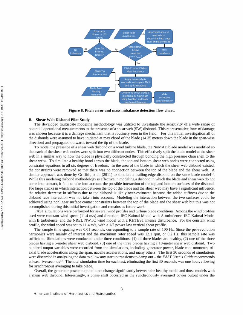
Figure 8. Pitch error and mass imbalance detection flow chart.

B. Shear Web Disbond Pilot Study The developed multiscale modeling methodology was utilized to investigate the sensitivity of a wide range of

potential operational measurements to the presence of a shear web (SW) disbond. This representative form of damage was chosen because it is a damage mechanism that is routinely seen in the field. For this initial investigation all of the disbonds were assumed to have initiated at max chord of the blade (14.35 meters down the blade in the span-wise direction) and propagated outwards toward the tip of the blade.

To model the presence of a shear web disbond on a wind turbine blade, the NuMAD blade model was modified so that each of the shear web nodes were split into two different nodes. This effectively split the blade model at the shear web in a similar way to how the blade is physically constructed through bonding the high pressure clam shell to the shear webs. To simulate a healthy bond across the blade, the top and bottom shear web nodes were connected using constraint equations in all six degrees of freedom. In the area of the blade in which the shear web disbond existed, the constraints were removed so that there was no connection between the top of the blade and the shear web. A similar approach was done by Griffith, et al. (2011) to simulate a trailing edge disbond on the same blade model12. While this modeling disbond methodology is effective in modeling a disbond in which the blade and shear web do not come into contact, it fails to take into account the possible interaction of the top and bottom surfaces of the disbond. For large cracks in which interaction between the top of the blade and the shear web may have a significant influence, the relative decrease in stiffness due to the disbond is likely over-estimated because the added stiffness due to the disbond face interaction was not taken into account. Modeling the interaction between the two surfaces could be achieved using nonlinear surface contact constraints between the top of the blade and the shear web but this was not accomplished during this initial investigation and remains as future work.

FAST simulations were performed for several wind profiles and turbine blade conditions. Among the wind profiles used were constant wind speed (11.4 m/s) and direction, IEC Kaimal Model with A turbulence, IEC Kaimal Model with B turbulence, and the NREL NWTC wind model with a KHTEST intense disturbance. For the constant wind profile, the wind speed was set to 11.4 m/s, with a 1/7 power law vertical shear profile.

The sample time spacing was 0.01 seconds, corresponding to a sample rate of 100 Hz. Since the per-revolution harmonics were mainly of interest and the maximum rotor speed was 12.1 rpm, or 0.2 Hz, this sample rate was sufficient. Simulations were conducted under three conditions: (1) all three blades are healthy, (2) one of the three blades having a 5-meter shear web disbond, (3) one of the three blades having a 10-meter shear web disbond. Two hundred output variables were recorded from the simulations, including generator power, blade root moments, tri-axial blade accelerations along the span, nacelle accelerations, and many others. The first 30 seconds of simulations were discarded in analyzing the data to allow any startup transients to damp out – the FAST User’s Guide recommends at least five seconds13. The total simulation time for each test, eliminating the first 30 seconds, was one hour, allowing for synchronous averaging to take place.

Overall, the generator power output did not change significantly between the healthy model and those models with a shear web disbond. Interestingly, a phase shift occurred in the synchronously averaged power output under the

No Imbalance

Generator Power or LSS

Torque

1p or 3p PS mag. largest?

Mean power below

expected given Vwind?

3p 1p Mass Imbalance

Pitch Error or Pitch + Mass Imbalance

No

Yes

Blade Tip Accelerations

Blade Root Pitching

Moments

Apply data analysis methods to compute RMS

and 1p PS response

Determine which blade is pitched & by how much

using baseline and blade-to-blade differences

Apply data analysis methods to

determine imbalance level and faulty blade

Blade Root Axial Forces

Make corrective

control decision


8

Dow

nloa

ded

by S

AN

DIA

NA

TIO

NA

L L

AB

OR

AT

OR

IES

on O

ctob

er 2

2, 2

014

| http

://ar

c.ai

aa.o

rg |

DO

I: 1

0.25

14/6

.201

4-07

14

presence of a SW disbond. However, the RMS power output did not change more than ~0.035% when the three turbine models were examined under the four different wind profiles.

For all of the following discussion, axial nacelle acceleration will refer to acceleration in the xs direction, vertical nacelle acceleration (or tower axis) will refer to acceleration in the ys direction, and transverse (or side-to-side) nacelle acceleration will refer to acceleration in the zs direction (see Figure 2a). For all wind cases, nacelle accelerations increased in all three directions with the presence of the shear web disbond. In addition, the percent changes were correlated with the extent of damage (i.e. length of the disbond). In addition, the xs and ys 1p response differences as well as the RMS differences in the zs direction indicated the presence and severity of disbond. However, no feature could be extracted to indicate which blade contained the damage based on nacelle-only measurements (no blade sensors). Figure 9a shows the 1p PS magnitude percent change of nacelle acceleration in the zs direction and Figure 9b shows the RMS percent change of nacelle acceleration in the ys direction.

(a) (b)

Figure 9. (a) 1p magnitude percent change of nacelle acceleration in the zs direction for shear web disbond; (b) RMS percent change of nacelle acceleration in the ys direction for shear web disbond

Now, usage of blade-mounted sensors is considered in addition to nacelle-mounted sensors. The blade tip

acceleration response in all three directions showed positive trends as the shear web disbond was introduced and increased in length. The 1p edge-wise blade acceleration response differences are shown in Figure 10a. These 1p response differences increased significantly with increasing shear web disbond (as much as a 25% increase for a 10 meter SW disbond). The blade tip span-wise acceleration 1p response differences (shown in Figure 10b) and flap-wise acceleration RMS response differences (shown in Figure 18c) also increase in the presence and increase of a shear web disbond. Note that the 1p magnitude percent change in the side-to-side nacelle acceleration was the most sensitive parameter to a shear web disbond, but the trend lines vary for the different wind profiles. On the other hand, the blade tip acceleration responses follow very similar trends for all four wind profiles.

(a) (b) (c)

Figure 10. (a) 1p magnitude percent change of edge-wise blade tip acceleration for shear web disbond; (b) 1p magnitude percent change of span-wise blade tip acceleration for shear web disbond; (c) RMS response

percent change of flap-wise blade tip acceleration for shear web disbond

The moment of the blade about its pitch axis at the blade root is another good indicator of a shear web disbond, as shown here. This moment can be measured using strain gages located at the root of each blade and this parameter was also shown to be a good indicator of pitch error, as shown in Section II. The blade root pitching moment 1p response differences (shown in Figure 11a) increase while the RMS response differences (shown in Figure 11b) are small and decrease with increased disbond length. The RMS response difference is very small, however the increase


9

Dow

nloa

ded

by S

AN

DIA

NA

TIO

NA

L L

AB

OR

AT

OR

IES

on O

ctob

er 2

2, 2

014

| http

://ar

c.ai

aa.o

rg |

DO

I: 1

0.25

14/6

.201

4-07

14

in the root pitching moment 1p response is expected since a shear web disbond would cause a reduction in flap-wise and torsional stiffness and the disbond originates at max chord, relatively close to the root of the blade. Both measurement sets also follow very similar trends for all four wind profiles as the shear web disbond is increased.

(a) (b)

Figure 12. (a) 1p magnitude percent change of blade root pitching moment for shear web disbond;(b) RMS response percent change of root blade pitching moment for shear web disbond

The results of these analyses can be synthesized into a flow chart, as shown in Figure 12, for detection of shear

web disbonds using a combination of sensors and analysis methods. The proposed strategy is to:

(1) Detect if a shear web disbond exists in one of the blades (2) Determine the severity of the shear web disbond (3) Notify turbine operator of the disbond and severity so that a repair can be scheduled or

coordinated with other maintenance

Figure 12. Shear web disbond detection flow chart

In the following two sections, an aerodynamic inflow sensitivity analysis is performed to further evaluate the

detection strategies for both shear web disbond (Figure 12) and rotor imbalance (Figure 8).


10

Dow

nloa

ded

by S

AN

DIA

NA

TIO

NA

L L

AB

OR

AT

OR

IES

on O

ctob

er 2

2, 2

014

| http

://ar

c.ai

aa.o

rg |

DO

I: 1

0.25

14/6

.201

4-07

14

IV. Rotor Imbalance Aerodynamic Sensitivity Analysis A comprehensive aerodynamic uncertainty analysis was conducted to evaluate the detection strategies developed

using operational measurements as features to assert the presence and severity of a pitch error or a mass imbalance. Although simultaneous pitch error and mass imbalance was investigated in the pilot study, this sensitivity analysis focuses on solely detecting either a pitch error or mass imbalance. 11,312 FAST simulations were performed to evaluate the robustness of the pitch error and mass imbalance detection strategies and examine their sensitivity to varying parameters including wind speed, horizontal shear, turbulence, and imbalance severity. All of the damage cases for both types of imbalance were applied the same way as in the pilot study. This section includes a variety of different sensitivity analyses that were conducted at various stages throughout the modeling and simulation processes.

For this sensitivity analysis, the parameters which were varied include the extent of damage and inflow conditions for the turbine. The NREL offshore 5-MW baseline wind turbine model and FAST were used to simulate the varying parameters. Table 2 shows the matrix of FAST simulations performed for the sensitivity analysis. Operational measurements were analyzed for a healthy turbine in addition to turbines with one of the three blades having a certain level of pitch error or mass imbalance. Mean wind speed, horizontal shear, and turbulence were among the aerodynamic parameters used in this study. For all of the wind profiles, a 1/7 power law vertical shear profile was applied. For all wind profiles, the wind speed was varied from 3 m/s to 25 m/s in 0.22 m/s increments (totaling 101 simulations per turbine damage type). Horizontal shear parameters of 0.3, 0.6, and 0.9 (or 30%, 60%, and 90% horizontal shear) were used (totaling 303 simulations per turbine damage type). The horizontal wind shear parameter is expressed as a linear spectrum of wind speed across the rotor disc. The horizontal wind shear parameter is ranged between -1 and 1, and it represents the wind speed at the blade tip on one side of the rotor minus the wind speed at the blade tip on the opposite side of the rotor, divided by the hub-height wind speed. The horizontal shear is measured in the direction perpendicular to the normally prevailing wind vector. The turbulence models used include the IEC Kaimal Model with A turbulence, the IEC Kaimal Model with B turbulence, and the NREL NWTC wind model with a KHTEST intense disturbance (totaling 303 simulations per turbine damage type).

Table 2. Number of FAST simulations run for each blade imbalance type. Pitch Error

(0o, 1o, 2o, 3o, 4o, 5o, 7.5o, 10o, 15o, 20o, 25o)

Mass Imbalance (G00, G06, G16, G40, G53)

Wind Speed (3 – 25 m/s) 1111 505 Horizontal Shear (30%, 60%,

90%) 3333 1515

Turbulence (A, B, KHTEST) 3333 1515

A. Analysis of Measurements Used for Pitch Error Detection Strategy Since the generator power was used to determine a blade pitch error in the pilot study, this parameter was once

again analyzed in order to determine if it can be used for the refined rotor imbalance detection strategy. The rotor azimuth position output from FAST was used as the reference signal for time synchronous averaging. The rotational resampling was performed in the same way as described in the pilot study. The azimuth signal was converted to radians, unwrapped and then the measurement signal was interpolated so that each revolution contained the same number of data samples with each sample corresponding to the same azimuth position of the rotor's rotation. Three revolutions of data blocks were averaged together. By using more than one revolution in the block size, the length of the block's time history could be increased which in turn increases the frequency resolution of the DFT of the time-averaged signal.

As expected, the generator power decreased in the presence of increasing pitch errors when varying the wind speed, horizontal shear, and turbulence wind profiles. As the wind speed increases beyond the turbine’s rated speed of 11.4 m/s, the generator power for the damage cases converge with the healthy case. In addition, the wind speed at which the two cases converge increases as the amount of pitch error is also increased. These results reinforce the importance of detecting an aerodynamic imbalance before it becomes severe. Figures 13 and 14 show the RMS power and percent change in power output for the laminar wind profile in the presence of a pitch error.


11

Dow

nloa

ded

by S

AN

DIA

NA

TIO

NA

L L

AB

OR

AT

OR

IES

on O

ctob

er 2

2, 2

014

| http

://ar

c.ai

aa.o

rg |

DO

I: 1

0.25

14/6

.201

4-07

14

Figure 13. RMS power output for each pitch error in varying wind speeds.

Figure 14. RMS percent change of power output for each pitch error in varying wind speeds.

B. Analysis of Measurements Used for Mass Imbalance Detection Strategy The blade root axial force was used to determine a blade mass imbalance in the pilot study, so this parameter was

again analyzed in order to determine if it can be used for the refined rotor imbalance detection strategy. The time synchronous averaging and rotational resampling were performed the same way as described in Section IV-A.

The blade root axial force again increased in the presence of increasing mass imbalances for all wind profiles. Up to the rated speed of the turbine, the RMS axial force diverged with wind speed as the mass imbalance increased. After the turbine reaches its rated speed, the blade root axial force differences remain constant. Figures 15 and 16 show the RMS blade root axial force differences for the laminar and A turbulence wind profiles in the presence of a mass imbalance.


12

Dow

nloa

ded

by S

AN

DIA

NA

TIO

NA

L L

AB

OR

AT

OR

IES

on O

ctob

er 2

2, 2

014

| http

://ar

c.ai

aa.o

rg |

DO

I: 1

0.25

14/6

.201

4-07

14

Figure 15. RMS blade root axial force for mass imbalance in varying wind speeds.

Figure 16. RMS percent change of blade root axial force for mass imbalance in A turbulence.

C. Summary of Rotor Imbalance Detection Strategy Refinements The results of the sensitivity analysis and key measurements have been used to refine the rotor imbalance detection

strategy. This strategy employs both blade and non-blade sensor measurements. Specifically, non-blade sensor measurements are used as the indicator for a pitch error and the blade sensors (strain gages at the blade root to measure the axial force) are used to detect a mass imbalance and its level of severity. The action strategy and flow chart have not changed; however, each rotor imbalance has been assigned thresholds corresponding to the severity of the imbalance, as shown below in Tables 3 and 4 for pitch error and mass imbalance, respectively.

Table 3. Pitch error damage state and corresponding feature used for classification State 1 (Healthy, 0o pitch error) Measured RMS power >= expected healthy RMS power State 2 (2o, 3o, 4o, 5o pitch errors) Greater than zero and less than 10% decrease in measured RMS power

State 3 (7.5o, 10o, 12.5o, 15o pitch errors) Greater than 10% and less than 51% decrease in measured RMS power State 4 (20o, 25o, and higher pitch errors) Greater than 51% decrease in measured RMS power

Table 4. Mass imbalance damage state and corresponding feature used for classification State 1 (Healthy, no mass imbalance) Measured blade axial force difference >= 300 N increase in expected

healthy blade axial force difference State 2 (G6.3 mass imbalance) Greater than or equal to 300 N and less than 950 N increase in

measured blade axial force difference State 3 (G16 mass imbalance) Greater than 950 N and less than 2300 N increase in measured blade

axial force difference State 4 (G40, G53, and higher mass imbalances) Greater than 2300 N increase in measured blade axial force difference

Probability of detection values were calculated for detecting the presence of a pitch error or mass imbalance in addition to detecting three different damage states which vary by severity. An optimal sensor configuration was used based on the developed rotor imbalance detection strategy: (1) power sensors for generator power measurement and (2) strain gages at each blade root for blade root axial force measurements. See Tables 3 and 4 for the damage state


13

Dow

nloa

ded

by S

AN

DIA

NA

TIO

NA

L L

AB

OR

AT

OR

IES

on O

ctob

er 2

2, 2

014

| http

://ar

c.ai

aa.o

rg |

DO

I: 1

0.25

14/6

.201

4-07

14

classifications of pitch error and mass imbalance, respectively. These damage state classifications were used for each FAST simulation and inflow condition. If the measurement at a given wind speed, profile, and damage state met the criteria described in the tables above, then it was deemed a success. Otherwise, it was deemed a failure. For example, the blade root axial force is extracted from the simulation for the 3.88 m/s laminar wind profile and for a turbine with a blade which has a G16 mass imbalance. If the blade root axial force difference is greater than 950 N and less than 2300 N, then the detection is a success and given a “1” value at that data point. If it does not meet the criteria, it is given a “0” value. The number of successes are then added up and that total is divided by the total number of simulations in that wind profile (101 simulations). The resultant percentage is the probability of detection for that damage state and wind profile. For state 2 through 4, the POD is calculated for the probability that the presence of damage is detected in addition to the classification for that damage class, respectively. Tables 5 and 6 show the POD values for detecting the presence of a pitch error or mass imbalance and then categorizing the damage into each damage case, respectively. The PODs were calculated over the entire wind speed range in addition to an enhanced wind speed range which optimizes the resulting POD value for accurate damage detection for all wind loading cases. In other words, the measurements, algorithms, and probability of detection calculations are only done within the wind speed range defined in the tables below. The optimized wind speed range and corresponding POD values are highlighted in green in the table. In addition, each POD value was weighted by the Weibull distribution to incorporate the frequency of each wind speed used within the analyzed range. The weighted pitch error POD results show that the developed algorithms are at least 96.28% successful for all of the FAST simulations except the turbulence cases for damage states 3 and 4. Since the weighted success rate of detecting the presence of a pitch error is 96.28% or higher, those pitch errors which fail to be classified in states 3 and 4 in turbulent conditions will still be detected as being in a damaged state. If the algorithm is unable to classify the pitch error severity, then another measurement will be made as soon as the inflow is not turbulent anymore. Inflow characteristics can be defined with an ultrasonic anemometer in order to determine the wind profile. As for mass imbalance, its PODs were 100% successful in the optimized wind speed range for all wind profiles.

Table 5. Probabilities of detection for pitch error

Table 6. Probabilities of detection for mass imbalance


14

Dow

nloa

ded

by S

AN

DIA

NA

TIO

NA

L L

AB

OR

AT

OR

IES

on O

ctob

er 2

2, 2

014

| http

://ar

c.ai

aa.o

rg |

DO

I: 1

0.25

14/6

.201

4-07

14

V. Shear Web Disbond Sensitivity Analysis A comprehensive aerodynamic uncertainty analysis was also conducted to evaluate the detection strategy

developed using operational measurements as features to assert the presence and severity of a shear web disbond (as described in the FY12 report). 4,949 FAST simulations were performed to evaluate the robustness of the shear web disbond detection strategy and examine its sensitivity to varying parameters including wind speed, horizontal shear, turbulence, and disbond length. All of the disbonds were assumed to have initiated at max chord of the blade (at the 14.35 meter span location) and propagated outwards toward the tip of the blade. This section includes a variety of different sensitivity analyses that were conducted at various stages throughout the modeling and simulation processes.

For this sensitivity analysis, the parameters which were varied include the extent of damage and inflow conditions for the turbine. The NREL offshore 5-MW baseline wind turbine model and FAST were used to simulate the varying parameters. Table 7 shows the matrix of FAST simulations performed for the sensitivity analysis. Operational measurements were analyzed for a healthy turbine in addition to turbines with one of the three blades containing a shear web disbond of 1, 2, 3, 4, 5, or 10 meters in length. Mean wind speed, horizontal shear, and turbulence were among the aerodynamic parameters used in this study. The wind profiles were defined as described for the rotor imbalance sensitivity analysis in Section IV.

Table 7. Number of FAST simulations run for each blade damage type.

Healthy 1m Disbond 2m Disbond 3m Disbond 4m Disbond 5m Disbond 10m Disbond Wind Speed (3 – 25 m/s) 101 101 101 101 101 101 101

Horizontal Shear (30%, 60%, 90%)

303 303 303 303 303 303 303

Turbulence (A, B,

KHTEST) 303 303 303 303 303 303 303

D. Shear Web Disbond Sensitivity and Structural Effects The shear web disbond damage cases are now expanded to include disbond lengths of 1, 2, 3, 4, 5, and 10 meters.

The stiffness values of each blade damage case were extracted from each section of their reduced order models. Figures 17 and 18 show the percent decreases in edge-wise, flap-wise, torsional, and axial stiffness, respectively. As expected, all four stiffness parameters decreased at the damage location as the disbond length was increased. The shear web disbond also had the largest effect on torsional stiffness, reiterating that measurements which are sensitive to the blade's torsional response will be good indicators that a shear web disbond is present.


15

Dow

nloa

ded

by S

AN

DIA

NA

TIO

NA

L L

AB

OR

AT

OR

IES

on O

ctob

er 2

2, 2

014

| http

://ar

c.ai

aa.o

rg |

DO

I: 1

0.25

14/6

.201

4-07

14

(a)

(b)

Figure 17. The percent decreases of the (a) flap-wise stiffness and (b) edge-wise stiffness values for varying

length disbonds for segments spaced along the length of the blade


16

Dow

nloa

ded

by S

AN

DIA

NA

TIO

NA

L L

AB

OR

AT

OR

IES

on O

ctob

er 2

2, 2

014

| http

://ar

c.ai

aa.o

rg |

DO

I: 1

0.25

14/6

.201

4-07

14

(a)

(b)

Figure 18. The percent decreases of the (a) torsional stiffness and (b) axial stiffness values for varying length disbonds for segments spaced along the length of the blade

E. Analysis of Measurements Used for Detection Strategy Analysis was once again applied to bladed and non-bladed sensors to compare the effectiveness and robustness of

the shear web disbond detection strategy described in Section III-B. All measurements outlined in the pilot study were examined to determine if any non-bladed sensors could be used for a refined detection strategy. From the


17

Dow

nloa

ded

by S

AN

DIA

NA

TIO

NA

L L

AB

OR

AT

OR

IES

on O

ctob

er 2

2, 2

014

| http

://ar

c.ai

aa.o

rg |

DO

I: 1

0.25

14/6

.201

4-07

14

variables analyzed from the FAST simulation outputs, those which displayed significant percentage changes in their RMS value or frequency response magnitude at the operating speed given a shear web disbond were identified as key measurement channels. The rotor azimuth position output from FAST was used as the reference signal for time synchronous averaging. The rotational resampling was performed in the same way as described in the pilot study. The azimuth signal was converted to radians, unwrapped and then the measurement signal was interpolated so that each revolution contained the same number of data samples with each sample corresponding to the same azimuth position of the rotor's rotation. Three revolutions of data blocks were averaged together. By using more than one revolution in the block size, the length of the block's time history could be increased which in turn increases the frequency resolution of the DFT of the time-averaged signal. The shear web disbond detection algorithms for the selected measurements all functioned in a similar way: detecting changes from baseline measurements either in the RMS response or 1p power spectral density magnitude.

Overall, the generator power did not change significantly in the presence of a shear web disbond when varying the wind speed, horizontal shear, and turbulence wind profiles. The power output experienced a few transients between the cut-in and rated speeds during the turbulent simulations, although all of the power output changes after the turbine reached the rated speed were negligible. Figure 19 shows the RMS percent change in power output for the laminar wind profile in the presence of a shear web disbond.

Figure 19. RMS percent change of power output for shear web disbond in varying wind speeds.

For all wind profiles and damage cases, the RMS value of the nacelle acceleration in all three directions increased

at the turbine's rated wind speed (11.4 m/s) or higher. As was seen in the pilot study, the transverse nacelle acceleration showed a clear RMS increase for all aerodynamic cases between the rated speed and approximately 20 m/s (shown in Figure 21). In addition, the nacelle accelerations increased as the shear web disbond length was increased. Figures 20 - 22 show the RMS percent change in nacelle acceleration in the axial, transverse, and vertical directions respectively. The 1p response magnitude was analyzed as well, but the trends of an increasing magnitude were not as apparent for all of the wind loading cases. Because these measurements were made at the nacelle hub, it is not possible to determine the problematic blade if one of the three blades has the shear web disbond. However, these measurements can be used to indicate that a shear web disbond is present and then trigger more sophisticated measurements to determine which blade has the disbond and the severity of the damage.


18

Dow

nloa

ded

by S

AN

DIA

NA

TIO

NA

L L

AB

OR

AT

OR

IES

on O

ctob

er 2

2, 2

014

| http

://ar

c.ai

aa.o

rg |

DO

I: 1

0.25

14/6

.201

4-07

14

Figure 20. RMS percent change of axial nacelle acceleration for shear web disbond in 60% horizontal

shear.

Figure 21. RMS percent change of transverse nacelle acceleration for shear web disbond in 60%

horizontal shear.


19

Dow

nloa

ded

by S

AN

DIA

NA

TIO

NA

L L

AB

OR

AT

OR

IES

on O

ctob

er 2

2, 2

014

| http

://ar

c.ai

aa.o

rg |

DO

I: 1

0.25

14/6

.201

4-07

14

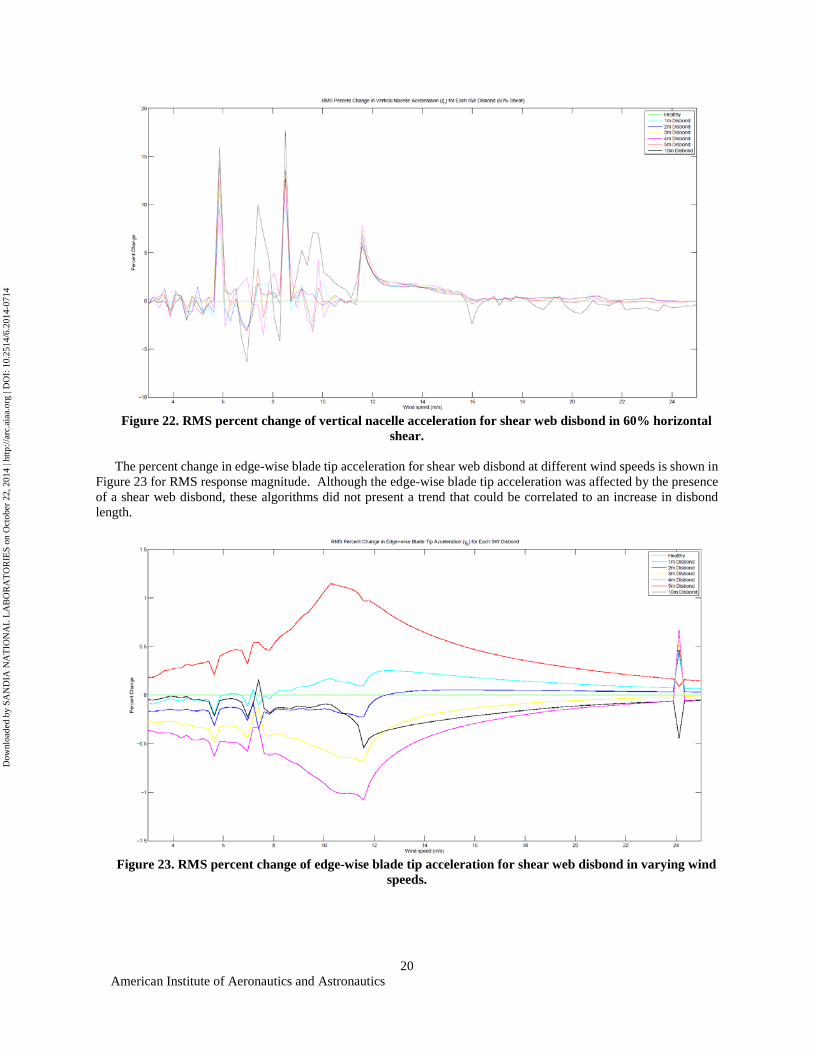
Figure 22. RMS percent change of vertical nacelle acceleration for shear web disbond in 60% horizontal

shear. The percent change in edge-wise blade tip acceleration for shear web disbond at different wind speeds is shown in

Figure 23 for RMS response magnitude. Although the edge-wise blade tip acceleration was affected by the presence of a shear web disbond, these algorithms did not present a trend that could be correlated to an increase in disbond length.

Figure 23. RMS percent change of edge-wise blade tip acceleration for shear web disbond in varying wind

speeds.


20

Dow

nloa

ded

by S

AN

DIA

NA

TIO

NA

L L

AB

OR

AT

OR

IES

on O

ctob

er 2

2, 2

014

| http

://ar

c.ai

aa.o

rg |

DO

I: 1

0.25

14/6

.201

4-07

14

The span-wise blade tip acceleration 1p response differences are shown in Figures 24 and 25. The plots show that when a shear web disbond was present, the 1p power spectrum response difference was always positive up to 18 m/s for all wind loading cases. Although there doesn't appear to be a trend that shows the severity of the damage, this measurement can serve as a good indicator that a shear web disbond is present.

Figure 24. 1p magnitude percent change of span-wise blade tip acceleration for shear web disbond in

varying wind speeds.

Figure 25. 1p magnitude percent change of span-wise blade tip acceleration for shear web disbond in A

turbulence.


21

Dow

nloa

ded

by S

AN

DIA

NA

TIO

NA

L L

AB

OR

AT

OR

IES

on O

ctob

er 2

2, 2

014

| http

://ar

c.ai

aa.o

rg |

DO

I: 1

0.25

14/6

.201

4-07

14

The flap-wise blade tip acceleration RMS response differences are shown in Figures 26 and 27. For all wind loading cases, there was a clear decrease in the RMS response at the turbine's rated speed (11/4 m/s) for shear web disbond lengths of 2 meters or greater. The trend of a decreased flap-wise blade tip acceleration RMS response was apparent at rated speed for all of the FAST simulations conducted in this study. In addition, the RMS response decreased as the shear web disbond length was increased. Therefore, this measurement can serve as a feature to indicate shear web disbond severity.

Figure 26. RMS percent change of flap-wise blade tip acceleration for shear web disbond in varying wind

speeds.

Figure 27. RMS percent change of flap-wise blade tip acceleration for shear web disbond in 90%

horizontal shear.


22

Dow

nloa

ded

by S

AN

DIA

NA

TIO

NA

L L

AB

OR

AT

OR

IES

on O

ctob

er 2

2, 2

014

| http

://ar

c.ai

aa.o

rg |

DO

I: 1

0.25

14/6

.201

4-07

14

Figures 28 and 29 show the blade root pitching moment 1p response differences for the laminar and B turbulence wind loading cases. For all of the wind cases up to a wind speed of 16 m/s, the 1p response increased for a 4 meter, 5 meter, and 10 meter shear web disbond. This measurement can be used as another indicator that a severe shear web disbond is present in one of the blades. The blade root pitching moment can be measured with strain gages located at the root of each blade.

Figure 28. 1p magnitude change of blade root pitching moment for shear web disbond in varying wind

speeds.

Figure 29. 1p magnitude change of blade root pitching moment for shear web disbond in B turbulence.


23

Dow

nloa

ded

by S

AN

DIA

NA

TIO

NA

L L

AB

OR

AT

OR

IES

on O

ctob

er 2

2, 2

014

| http

://ar

c.ai

aa.o

rg |

DO

I: 1

0.25

14/6

.201

4-07

14

F. Summary of Shear Web Disbond Detection Strategy Refinements The results of the sensitivity analysis and key measurements have been used to refine the shear web disbond

detection strategy flowchart originally shown in Figure 30. This strategy employs both blade and non-blade sensor measurements. Specifically, non-blade sensor measurements are used as the first indicator that a shear web disbond may be present and the blade sensors are used to confirm that the damage is present and its level of severity. Using a single sensor measurement to first identify potential damage will drastically reduce the necessary amount of processing and data flow in situ. The same action strategy will be used, as shown below:

(1) Detect if a shear web disbond exists in one of the blades (2) Determine the severity of the shear web disbond (3) Notify turbine operator of the disbond and severity so that a repair can be scheduled or coordinated with other

maintenance

Figure 30. Refined shear web disbond detection flow chart.

Probability of detection values were calculated for detecting the presence of a shear web disbond in addition to detecting three different damage states which vary by severity. An optimal sensor configuration was used based on the developed shear web disband detection strategy: (1) single DC tri-axial accelerometer at the nacelle hub and a DC tri-axial accelerometer at each blade tip for acceleration measurements and (2) strain gages at each blade root for blade root pitching moment measurements. See Table 8 below for the damage state classifications of shear web disbond. State 2 refers to a 1-2 meter disbond, state 3 is a 3-5 meter disbond, and state 4 is a disbond of 10 meters or more. The POD values were calculated as described in Section IV-C. Table 9 shows the POD values for detecting the presence of a disbond and then categorizing the damage into each damage case, respectively. The PODs were calculated over the entire wind speed range in addition to an enhanced wind speed range which optimizes the resulting POD value for accurate damage detection for all wind loading cases. The optimized wind speed range and corresponding POD values are highlighted in green in the table. In addition, each POD value was also weighted by the Weibull distribution to incorporate the frequency of each wind speed used within the analyzed range. The POD results show that the developed algorithms are 100% successful for all of the laminar, 30% horizontal shear, and 60% horizontal shear FAST simulations. The POD values are also ~75% or greater for all but the 90% horizontal shear simulations. There is a large decrease in that probability of detection because the aerodynamic loading greatly influences the transverse nacelle acceleration response and this feature becomes the dominating feature at that measurement location rather than


24

Dow

nloa

ded

by S

AN

DIA

NA

TIO

NA

L L

AB

OR

AT

OR

IES

on O

ctob

er 2

2, 2

014

| http

://ar

c.ai

aa.o

rg |

DO

I: 1

0.25

14/6

.201

4-07

14

a shear web disbond in one of the three blades. In the real world, however, a 90% horizontal shear wind profile does not occur nearly as often as the laminar and other shear wind profiles.

Table 8. Shear web disbond damage state and corresponding feature used for classification State 1 (Healthy, no disbond) 1% increase in measured RMS transverse nacelle acceleration versus

expected healthy RMS transverse nacelle acceleration State 2 (1, 2 meter disbond) 1% increase in measured RMS transverse nacelle acceleration, less

than 0.5% increase in 1p blade root pitching moment State 3 (3, 4, 5 meter disbond) Greater than 0.5% and less than 5% increase in 1p blade root pitching

moment State 4 (10 meter disbond or longer) Greater than 5% increase in 1p blade root pitching moment

Table 9. Probabilities of detection for shear web disbond

VI. Conclusions A multiscale methodology12 has been expanded for the investigation and development of structural health and

prognostics management (SHPM) methods for offshore wind turbines. The method utilizes the propagation of damage from a high fidelity component level model up to a reduced order model of a full turbine so that the changes in the turbine’s operational responses can be examined. Furthermore, these full turbine simulations can be used to replicate fault mechanisms such as pitch error and estimate the loads on the turbine blades which can then be propagated back to the high fidelity model to allow for further local analyses to be conducted. By investigating the effects of damage on multiple scales, the developed methodology takes advantage of available software to investigate the underlying physical changes that occur as a result of damage/faults on both a local and global level which leads to the identification of operational responses that are most sensitive to these physical changes. In turn, fault detection strategies have been developed to help optimize operations and maintenance schemes.

This paper has described the application of the developed methodology to investigate rotor imbalance and shear web disbond and their sensitivities to inflow conditions on an offshore 5-MW wind turbine. The 61.5 meter blade model was developed in SNL’s NuMAD software and exported to ANSYS where the shear web disbond was simulated by separating the nodes of the shear web from the blade at the location of the disbond. The reduced order blade models with varying levels of damage were included into a model of an offshore turbine on a fixed monopole in 20 meters of water. The response of these offshore turbine models with varying levels of damage/imbalance was then simulated in FAST over a wide range of wind speed, horizontal shear, and turbulence. From these simulations the detection strategies developed in the pilot study could be updated and robust probabilities of detection were derived as an algorithm success metric. For all three fault mechanisms, the probability of detection was 96% or higher for the optimized wind speed ranges including the laminar, 30% horizontal shear, and 60% horizontal shear conditions. Additional research work has been performed to examine how the structural health of each turbine could be used to optimize the operation and maintenance practices of an offshore wind plant. A cost model is being developed to investigate the operations and maintenance costs due to given faults/damage. The combination of the repair cost information and the structural health of each turbine could be utilized in the optimization of damage mitigating control strategies and maintenance schedules to reduce the operations and maintenance costs associated with running an offshore wind energy plant.


25

Dow

nloa

ded

by S

AN

DIA

NA

TIO

NA

L L

AB

OR

AT

OR

IES

on O

ctob

er 2

2, 2

014

| http

://ar

c.ai

aa.o

rg |

DO

I: 1

0.25

14/6

.201

4-07

14

Acknowledgments We would like to acknowledge Todd Griffith, Sandia National Laboratories, as the contract monitor for this work

and the U.S. Department of Energy for their continuing support of the wind energy research efforts being performed at Purdue University.

References 1A.C. Levitt, W. Kempton, A.P. Smith, W. Musial and J. Firestone, “Pricing offshore wind power.” Energy Policy (In Press)

2011. 2W. Musial and B. Ram, Large-Scale Offshore Wind Energy for the United States: Assessment of Opportunities and Barriers,

NREL Report No. TP-500-49229, Golden, CO, September 2010 1R. Wiser and M. Bolinger, 2010 Wind Technologies Market Report, Lawrence Berkeley

National Laboratory: Lawrence Berkeley National Laboratory. LBNL Paper LBNL-4820E, June 2011. 3B. Snyder and M.J. Kaiser, “Ecological and economic cost-benefit analysis of offshore wind energy.” Renewable Energy

34(6), pp. 1567-1578, 2009. 4G. van Bussel, A.R. Henderson, C.A. Morgan, B. Smith, R. Barthelmie, K. Argyriadis, A. Arena, G. Niklasson, and E. Peltola,

“State of the Art and Technology Trends for Offshore Wind Energy: Operation and Maintenance Issues,” Offshore Wind Energy EWEA Special Topic Conference, Brussels, Belgium, December 2001.

5L.W.M.M. Rademakers, H. Braam, M.B. Zaaiger, and G.J.W. van Bussel, “Assessment and optimisation of operation and maintenance of offshore wind turbines,” in Proceedings of the European Wind Energy Conference, Madrid, Span, June 2003.

6Y. Amirat, M.E.H Benbouzid, B. Bensaker, and R. Wamkeue, “Condition monitoring and fault diagnosis in wind energy conversion systems: a review.” In Proceedings 2007 IEEE International Electric Machines and Drives Conference, Vol 2., pp. 1434-1439, 2007.

7J. Nilsson and L. Bertling, “Maintenance management of wind power systems using condition monitoring systems – Life cycle cost analaysis for two case studies,” IEEE Transactions on Energy Conversion 22(1), pp. 223-229, 2007.

8C.C. Ciang, J.R. Lee, and H.J. Bang, “Structural health monitoring for a wind turbine system: a review of damage detection methods.” Measurement Science and Technology 19(12), pp. 1-20, 2008.

9F. Besnard, K. Fischer, and L. Bertling, “Reliability-centred asset maintenance – A step towards enhanced reliability availability and profitability of wind power plants” in 2010 IEEE PES Innovative Smart Grid Technologies Conference Europe (ISGT Europe), 2010.

10Z. Hameed, S.H. Ahn, and Y.M. Cho, “Practical aspects of a condition monitoring system for a wind turbine with emphasis on its design, system architecture, testing and installation,” Renewable Energy, 35(5), pp. 879-894, May 2010.

11J. Jonkman, S. Butterfield, W. Musial, and G. Scott, "Definition of a 5-MW Reference Wind Turbine for Offshore System Development," NREL/TP-500-38060, Golden, CO: National Renewable Energy Laboratory, February 2009.

12D.T. Griffith, N. Yoder, B. Resor, J. White, and J. Paquette, , “Structural Health and Prognostics Management for Offshore Wind Turbines: An Initial Roadmap,” SAND2012-10109, Sandia National Laboratories; Albuquerque, NM, Printed December 2012.

13J. Jonkman and L. Buhl, “FAST User’s Guide,” NREL/EL-500-38230, Golden, CO: National Renewable Energy Laboratory, August 2005.

14J. Losi, and E. Becker, "Imbalance: A danger to components," Erneuerbare Energien, August 2009. 15J. Giebhardt and WP7 Partners, “Condition Monitoring for Wind Turbines ‘State of the Art’ Report,” Kassel, Germany:

European Commission, 2007. 16M. MaCamhaoil, “Bruel & Kjaer Application Notes: Static and Dynamic Balancing of Rigid Rotors,” n.d.

http://www.bksv.com/doc/bo0276.pdf (accessed March 2012). 17Moog Incorporated, Rotor Monitoring Systems, June 2011. http://www.moog.com/literature/ICD/Moog-Wind-Rotor-

Monitoring-System-Overview-en.pdf (accessed March 13, 2012). 18J.P. Borg and R.H. Kirchoff, "Mass and Aerodynamic Imbalance of a Horizontal Axis Wind Turbine," Journal of Solar Energy

Engineering 120 (Feburary 1998): 66-74. 19Y. Nam, T. Yoon, K. Kim, and H. Cuong, 41. “Estimation of a Nacelle Dynamic Motion of a Wind Turbine,” Control,

Automation, Robotics and Vision, 2008, ICARCV 2008. 10th International Conference on , pp. 1017-1020, 2008. 20IEC 61400-1, “Wind turbine generator systems-Part 1: Safety requirements,” 2nd edition, Geneva,

Switzerland: International Electrotechnical Commission, 1999. 21B.J. Jonkman and L. Kilcher, “TurbSim User’s Guide: Version 1.06.00,” NREL/TP-xxx-xxxx (Draft Version), Golden, CO:

National Renewable Energy Laboratory, September 2012. 22D.J. Malcolm and D.L. Laird, "Extraction of Equivalent Beam Properties from Blade Models." Wind Energy, 2007, 10,

135-137. 23J. Kusnick. Rotor Blade Operational Data Analysis Methods and Applications for Condition Monitoring of Vertical and

Horizontal Axis Wind Turbines. Master's Thesis, West Lafayette, IN: Purdue University, 2012. 24N. Myrent, J. Kusnick, N. Barrett, D.E. Adams, and D.T. Grifith, , “Structural Health and Prognostics Management for

Offshore Wind Turbines: Case Studies of Rotor Fault and Blade Damage with Initial O&M Cost Modeling,” SAND2013-2735, Sandia National Laboratories; Albuquerque, NM, Printed April 2013.


26

Dow

nloa

ded

by S

AN

DIA

NA

TIO

NA

L L

AB

OR

AT

OR

IES

on O

ctob

er 2

2, 2

014

| http

://ar

c.ai

aa.o

rg |

DO

I: 1

0.25

14/6

.201

4-07

14

25D.T. Griffith, N. Yoder, B. Resor, J. White, and J. Paquette, “Structural health and prognostics management for the enhancement of offshore wind turbine operations and maintenance strategies.” Wind Energy. DOI: 10.1002/we. 1665

26N. Myrent, J. Kusnick, D.E. Adams, and D.T. Griffith, “Pitch Error and Shear Web Disbond Detection on Wind Turbine Blades for Offshore Structural Health and Prognostics Management,” 54th AIAA/ASME/ASCE/AHS Structures, Structural Dynamics, and Materials Conference, Boston, Massachusetts, April 2013.


27

Dow

nloa

ded

by S

AN

DIA

NA

TIO

NA

L L

AB

OR

AT

OR

IES

on O

ctob

er 2

2, 2

014

| http

://ar

c.ai

aa.o

rg |

DO

I: 1

0.25

14/6

.201

4-07

14

aerodynamic sensitivity analysis of rotor imbalance and...

Documents