aerodynamic background - cornell - cornell university · pdf filechapter 2 aerodynamic...

Chapter 2

Aerodynamic Background

Flight dynamics deals principally with the response of aerospace vehicles to perturbationsin their flight environments and to control inputs. In order to understand this response,it is necessary to characterize the aerodynamic and propulsive forces and moments actingon the vehicle, and the dependence of these forces and moments on the flight variables,including airspeed and vehicle orientation. These notes provide a simplified summary ofimportant results from aerodynamics that can be used to characterize these dependencies.

2.1 Introduction

Flight dynamics deals with the response of aerospace vehicles to perturbations in their flight environ-ments and to control inputs. Since it is changes in orientation (or attitude) that are most important,these responses are dominated by the generated aerodynamic and propulsive moments. For mostaerospace vehicles, these moments are due largely to changes in the lifting forces on the vehicle (asopposed to the drag forces that are important in determining performance). Thus, in some ways,the prediction of flight stability and control is easier than the prediction of performance, since theselifting forces can often be predicted to within sufficient accuracy using inviscid, linear theories.

In these notes, I attempt to provide a uniform background in the aerodynamic theories that can beused to analyze the stability and control of flight vehicles. This background is equivalent to thatusually covered in an introductory aeronautics course, such as one that might use the text by Shevell[6]. This material is often reviewed in flight dynamics texts; the material presented here is derived,in part, from the material in Chapter 1 of the text by Seckel [5], supplemented with some of thematerial from Appendix B of the text by Etkin & Reid [3]. The theoretical basis for these lineartheories can be found in the book by Ashley & Landahl [2].

11

12 CHAPTER 2. AERODYNAMIC BACKGROUND

c(y)

b/2

y

x

ctip

Λ0

rootc

Figure 2.1: Planform geometry of a typical lifting surface (wing).

2.2 Lifting surface geometry and nomenclature

We begin by considering the geometrical parameters describing a lifting surface, such as a wing orhorizontal tail plane. The projection of the wing geometry onto the x-y plane is called the wingplanform. A typical wing planform is sketched in Fig. 2.1. As shown in the sketch, the maximumlateral extent of the planform is called the wing span b, and the area of the planform S is called thewing area.

The wing area can be computed if the spanwise distribution of local section chord c(y) is knownusing

S =

∫ b/2

−b/2

c(y) dy = 2

∫ b/2

0

c(y) dy, (2.1)

where the latter form assumes bi-lateral symmetry for the wing (the usual case). While the spancharacterizes the lateral extent of the aerodynamic forces acting on the wing, the mean aerodynamic

chord c̄ characterizes the axial extent of these forces. The mean aerodynamic chord is usuallyapproximated (to good accuracy) by the mean geometric chord

c̄ =2

S

∫ b/2

0

c2 dy (2.2)

The dimensionless ratio of the span to the mean chord is also an important parameter, but insteadof using the ratio b/c̄ the aspect ratio of the planform is defined as

AR ≡b2

S(2.3)

Note that this definition reduces to the ratio b/c for the simple case of a wing of rectangular planform(having constant chord c).

2.2. LIFTING SURFACE GEOMETRY AND NOMENCLATURE 13

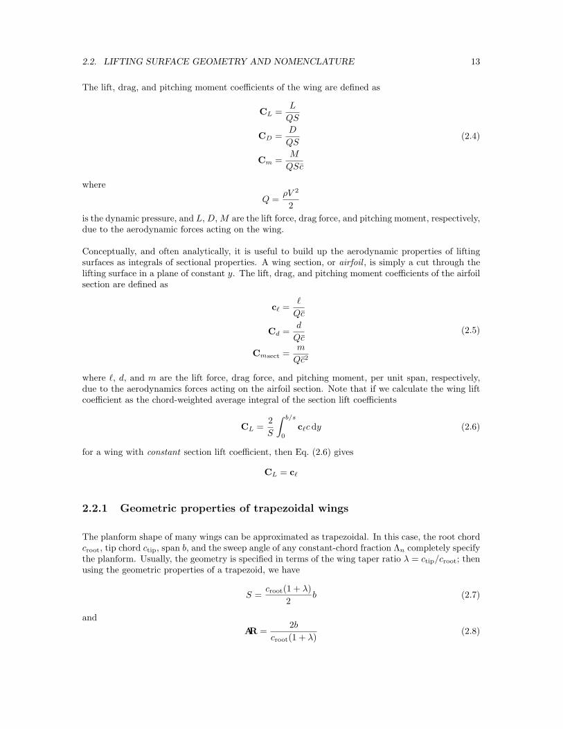
The lift, drag, and pitching moment coefficients of the wing are defined as

CL =L

QS

CD =D

QS

Cm =M

QSc̄

(2.4)

where

Q =ρV 2

2

is the dynamic pressure, and L, D, M are the lift force, drag force, and pitching moment, respectively,due to the aerodynamic forces acting on the wing.

Conceptually, and often analytically, it is useful to build up the aerodynamic properties of liftingsurfaces as integrals of sectional properties. A wing section, or airfoil , is simply a cut through thelifting surface in a plane of constant y. The lift, drag, and pitching moment coefficients of the airfoilsection are defined as

cℓ =ℓ

Qc̄

Cd =d

Qc̄

Cmsect =m

Qc̄2

(2.5)

where ℓ, d, and m are the lift force, drag force, and pitching moment, per unit span, respectively,due to the aerodynamics forces acting on the airfoil section. Note that if we calculate the wing liftcoefficient as the chord-weighted average integral of the section lift coefficients

CL =2

S

∫ b/s

0

cℓcdy (2.6)

for a wing with constant section lift coefficient, then Eq. (2.6) gives

CL = cℓ

2.2.1 Geometric properties of trapezoidal wings

The planform shape of many wings can be approximated as trapezoidal. In this case, the root chordcroot, tip chord ctip, span b, and the sweep angle of any constant-chord fraction Λn completely specifythe planform. Usually, the geometry is specified in terms of the wing taper ratio λ = ctip/croot; thenusing the geometric properties of a trapezoid, we have

S =croot(1 + λ)

2b (2.7)

and

AR =2b

croot(1 + λ)(2.8)


camber (mean) line

chord line

V

−α

α

0

chord, c

zero−lift line

Figure 2.2: Geometry of a typical airfoil section.

The local chord is then given as a function of the span variable by

c = croot

[

1 − (1 − λ)2y

b

]

(2.9)

and substitution of this into Eq. (2.2) and carrying out the integration gives

c̄ =2(1 + λ + λ2)

3(1 + λ)croot (2.10)

The sweep angle of any constant-chord fraction line can be related to that of the leading-edge sweepangle by

AR tan Λn = AR tan Λ0 − 4n1 − λ

1 + λ(2.11)

where 0 ≤ n ≤ 1 is the chord fraction (e.g., 0 for the leading edge, 1/4 for the quarter-chord line,etc.). Finally, the location of any chord-fraction point on the mean aerodynamic chord, relative tothe wing apex, can be determined as

x̄n =2

S

∫ b/2

0

xncdy =2

S

∫ b/2

0

(ncroot + y tan Λn) dy

=3(1 + λ)c̄

2(1 + λ + λ2)

{

n +

(

1 + 2λ

12

)

AR tan Λn

}(2.12)

Alternatively, we can use Eq. (2.11) to express this result in terms of the leading-edge sweep as

x̄n

c̄= n +

(1 + λ)(1 + 2λ)

8(1 + λ + λ2)AR tan Λ0 (2.13)

Substitution of n = 0 (or n = 1/4) into either Eq. (2.12) or Eq. (2.13) gives the axial location of theleading edge (or quarter-chord point) of the mean aerodynamic chord relative to the wing apex.

2.3 Aerodynamic properties of airfoils

The basic features of a typical airfoil section are sketched in Fig. 2.2. The longest straight line fromthe trailing edge to a point on the leading edge of the contour defines the chord line. The lengthof this line is called simply the chord c. The locus of points midway between the upper and lowersurfaces is called the mean line, or camber line. For a symmetric airfoil, the camber and chord linescoincide.

2.3. AERODYNAMIC PROPERTIES OF AIRFOILS 15

For low speeds (i.e., Mach numbers M << 1), and at high Reynolds numbers Re = V c/ν >> 1,the results of thin-airfoil theory predict the lifting properties of airfoils quite accurately for angles ofattack not too near the stall. Thin-airfoil theory predicts a linear relationship between the sectionlift coefficient and the angle of attack α of the form

cℓ = a0 (α − α0) (2.14)

as shown in Fig. 2.3. The theory also predicts the value of the lift-curve slope

a0 =∂cℓ

∂α= 2π (2.15)

Thickness effects (not accounted for in thin-airfoil theory) tend to increase the value of a0, whileviscous effects (also neglected in the theory) tend to decrease the value of a0. The value of a0 forrealistic conditions is, as a result of these counter-balancing effects, remarkably close to 2π for mostpractical airfoil shapes at the high Reynolds numbers of practical flight.

The angle α0 is called the angle for zero lift , and is a function only of the shape of the camber line.Increasing (conventional, sub-sonic) camber makes the angle for zero lift α0 increasingly negative.For camber lines of a given family (i.e., shape), the angle for zero lift is very nearly proportional tothe magnitude of camber – i.e., to the maximum deviation of the camber line from the chord line.

A second important result from thin-airfoil theory concerns the location of the aerodynamic center .The aerodynamic center of an airfoil is the point about which the pitching moment, due to thedistribution of aerodynamic forces acting on the airfoil surface, is independent of the angle of attack.Thin-airfoil theory tells us that the aerodynamic center is located on the chord line, one quarter ofthe way from the leading to the trailing edge – the so-called quarter-chord point. The value of thepitching moment about the aerodynamic center can also be determined from thin-airfoil theory, butrequires a detailed calculation for each specific shape of camber line. Here, we simply note that,for a given shape of camber line the pitching moment about the aerodynamic center is proportionalto the amplitude of the camber, and generally is negative for conventional subsonic (concave down)camber shapes.

It is worth emphasizing that thin-airfoil theory neglects the effects of viscosity and, therefore, cannotpredict the behavior of airfoil stall, which is due to boundary layer separation at high angles of attack.Nevertheless, for the angles of attack usually encountered in controlled flight, it provides a very usefulapproximation for the lift.

Angle of attack,

Thin−airfoil theory

Stall

α 0

Lift

coef

ficie

nt, C

l

α

2π

Figure 2.3: Airfoil section lift coefficient as a function of angle of attack.


Figure 2.4: Airfoil lift and moment coefficients as a function of angle of attack; wind tunnel data fortwo cambered airfoil sections. Data from Abbott & von Doenhoff [1].

Finally, wind tunnel data for two cambered airfoil sections are presented in Fig. 2.4. Both airfoilshave the same thickness distributions and camber line shapes, but the airfoil on the right has twiceas much camber as the one on the left (corresponding to 4 per cent chord, versus 2 per cent for theairfoil on the left). The several curves correspond to Reynolds numbers ranging from Re = 3 × 106

to Re = 9×106, with the curves having larger values of cℓmax corresponding to the higher Reynoldsnumbers. The outlying curves in the plot on the right correspond to data taken with a 20 per centchord split flap deflected (and are not of interest here).

Note that these data are generally consistent with the results of thin-airfoil theory. In particular:

1. The lift-curve slopes are within about 95 per cent of the value of a0 = 2π over a significantrange of angles of attack. Note that the angles of attack in Fig. 2.4 are in degrees, whereasthe a0 = 2π is per radian;

2. The angle for zero lift of the section having the larger camber is approximately twice that ofthe section having the smaller camber; and

3. The moment coefficients measured about the quarter-chord point are very nearly independentof angle of attack, and are roughly twice as large for the airfoil having the larger camber.

2.4. AERODYNAMIC PROPERTIES OF FINITE WINGS 17

2.4 Aerodynamic properties of finite wings

The vortex structures trailing downstream of a finite wing produce an induced downwash field nearthe wing which can be characterized by an induced angle of attack

αi =CL

πeAR(2.16)

For a straight (un-swept) wing with an elliptical spanwise loading, lifting-line theory predicts thatthe induced angle of attack αi is constant across the span of the wing, and the efficiency factor

e = 1.0. For non-elliptical span loadings, e < 1.0, but for most practical wings αi is still nearlyconstant across the span. Thus, for a finite wing lifting-line theory predicts that

CL = a0 (α − α0 − αi) (2.17)

where a0 is the wing section lift-curve slope and α0 is the angle for zero lift of the section. SubstitutingEq. (2.16) and solving for the lift coefficient gives

CL =a0

1 + a0

πeAR

(α − α0) = a(α − α0) (2.18)

whence the wing lift-curve slope is given by

a =∂CL

∂α=

a0

1 + a0

πeAR

(2.19)

Lifting-line theory is asymptotically correct in the limit of large aspect ratio, so, in principle,Eq. (2.18) is valid only in the limit as AR → ∞. At the same time, slender-body theory is valid inthe limit of vanishingly small aspect ratio, and it predicts, independently of planform shape, thatthe lift-curve slope is

a =πAR

2(2.20)

Note that this is one-half the value predicted by the limit of the lifting-line result, Eq. (2.19), asthe aspect ratio goes to zero. We can construct a single empirical formula that contains the correctlimits for both large and small aspect ratio of the form

a =πAR

1 +

√

1 +(

πAR

a0

)2(2.21)

A plot of this equation, and of the lifting-line and slender-body theory results, is shown in Fig. 2.5.

Equation (2.21) can also be modified to account for wing sweep and the effects of compressibility. Ifthe sweep of the quarter-chord line of the planform is Λc/4, the effective section incidence is increasedby the factor 1/ cos Λc/4, relative to that of the wing,1while the dynamic pressure of the flow normalto the quarter-chord line is reduced by the factor cos2 Λc/4. The section lift-curve slope is thusreduced by the factor cos Λc/4, and a version of Eq. (2.21) that accounts for sweep can be written

a =πAR

1 +

√

1 +(

πAR

a0 cos Λc/4

)2(2.22)

1This factor can best be understood by interpreting a change in angle of attack as a change in vertical velocity

∆w = V∞∆α.


0

0.2

0.4

0.6

0.8

1

0 2 4 6 8 10 12 14 16

Lifting-lineSlender-body

Empirical

Aspect ratio, b2/S

Norm

alized

lift

-curv

esl

ope,

a

2π

Figure 2.5: Empirical formula for lift-curve slope of a finite wing compared with lifting-line andslender-body limits. Plot is constructed assuming a0 = 2π.

Finally, for subcritical (M∞ < Mcrit) flows, the Prandtl-Glauert similarity law for airfoil sectionsgives

a2d =a0

√

1 − M2∞

(2.23)

where M∞ is the flight Mach number. The Goethert similarity rule for three-dimensional wingsmodifies Eq. (2.22) to the form

a =πAR

1 +

√

1 +(

πAR

a0 cos Λc/4

)2(

1 − M2∞

cos2 Λc/4

)

(2.24)

In Eqs. (2.22), (2.23) and (2.24), a0 is, as earlier, the incompressible, two-dimensional value of thelift-curve slope (often approximated as a0 = 2π). Note that, according to Eq. (2.24) the lift-curveslope increases with increasing Mach number, but not as fast as the two-dimensional Prandtl-Glauertrule suggests. Also, unlike the Prandtl-Glauert result, the transonic limit (M∞ cos Λc/4 → 1.0) isfinite and corresponds (correctly) to the slender-body limit.

So far we have described only the lift-curve slope a = ∂CL/∂α for the finite wing, which is itsmost important parameter as far as stability is concerned. To determine trim, however, it is alsoimportant to know the value of the pitching moment at zero lift (which is, of course, also equal tothe pitching moment about the aerodynamic center). We first determine the angle of attack forwing zero lift. From the sketch in Fig. 2.6, we see that the angle of attack measured at the wingroot corresponding to zero lift at a given section can be written

− (α0)root = ǫ − α0 (2.25)

where ǫ is the geometric twist at the section, relative to the root. The wing lift coefficient can thenbe expressed as

CL =2

S

∫ b/2

0

a [αr − (α0)root] cdy =2a

S

[

S

2αr +

∫ b/2

0

(ǫ − α0) cdy

]

(2.26)

2.5. FUSELAGE CONTRIBUTION TO PITCH STIFFNESS 19

−α

ε

−α0

root chord

local chord

local zero−lift line0 )

root

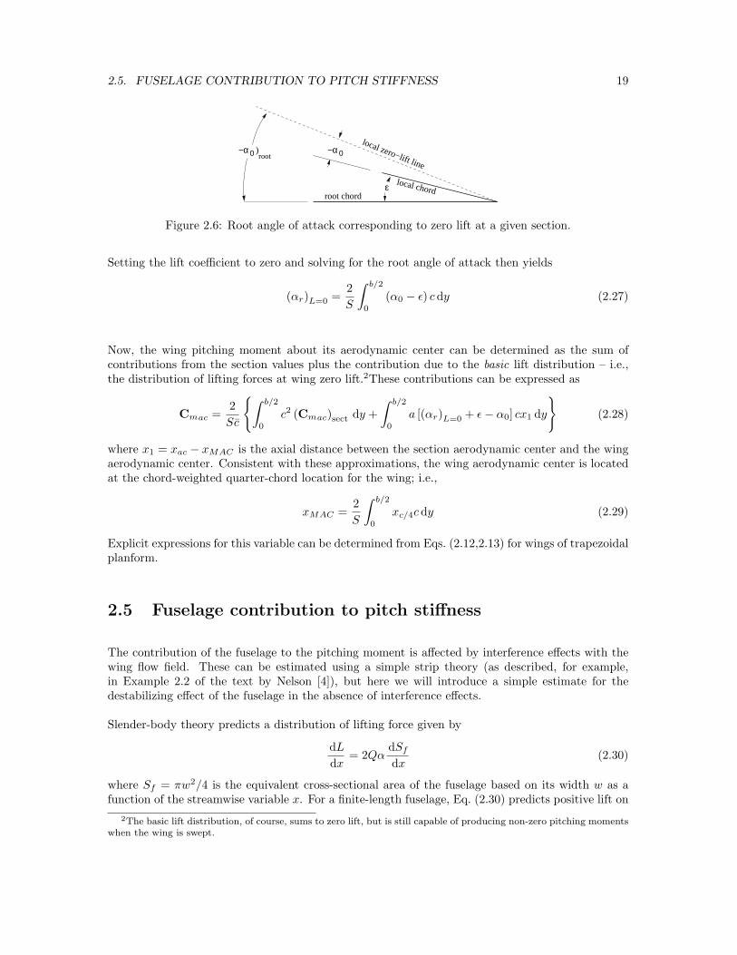
Figure 2.6: Root angle of attack corresponding to zero lift at a given section.

Setting the lift coefficient to zero and solving for the root angle of attack then yields

(αr)L=0 =2

S

∫ b/2

0

(α0 − ǫ) cdy (2.27)

Now, the wing pitching moment about its aerodynamic center can be determined as the sum ofcontributions from the section values plus the contribution due to the basic lift distribution – i.e.,the distribution of lifting forces at wing zero lift.2These contributions can be expressed as

Cmac =2

Sc̄

{

∫ b/2

0

c2 (Cmac)sect dy +

∫ b/2

0

a [(αr)L=0 + ǫ − α0] cx1 dy

}

(2.28)

where x1 = xac − xMAC is the axial distance between the section aerodynamic center and the wingaerodynamic center. Consistent with these approximations, the wing aerodynamic center is locatedat the chord-weighted quarter-chord location for the wing; i.e.,

xMAC =2

S

∫ b/2

0

xc/4cdy (2.29)

Explicit expressions for this variable can be determined from Eqs. (2.12,2.13) for wings of trapezoidalplanform.

2.5 Fuselage contribution to pitch stiffness

The contribution of the fuselage to the pitching moment is affected by interference effects with thewing flow field. These can be estimated using a simple strip theory (as described, for example,in Example 2.2 of the text by Nelson [4]), but here we will introduce a simple estimate for thedestabilizing effect of the fuselage in the absence of interference effects.

Slender-body theory predicts a distribution of lifting force given by

dL

dx= 2Qα

dSf

dx(2.30)

where Sf = πw2/4 is the equivalent cross-sectional area of the fuselage based on its width w as afunction of the streamwise variable x. For a finite-length fuselage, Eq. (2.30) predicts positive lift on

2The basic lift distribution, of course, sums to zero lift, but is still capable of producing non-zero pitching moments

when the wing is swept.


the forward part of the fuselage (where Sf is generally increasing), and negative lift on the rearwardpart (where Sf is generally decreasing), but the total lift is identically zero (since Sf (0) = Sf (ℓf ) = 0,where ℓf is the fuselage length).

Since the total lift acting on the fuselage is zero, the resulting force system is a pure couple, and thepitching moment will be the same, regardless of the reference point about which it is taken. Thus,e.g., taking the moment about the fuselage nose (x = 0), we have

Mf = −

∫ ℓf

0

xdL = −2Qα

∫ ℓf

0

xdSf = 2Qα

∫ ℓf

0

Sf dx = 2QαV (2.31)

where V is the volume of the “equivalent” fuselage (i.e., the body having the same planform as theactual fuselage, but with circular cross-sections). The fuselage contribution to the vehicle pitchingmoment coefficient is then

Cm =Mf

QSc̄=

2V

Sc̄α (2.32)

and the corresponding pitch stiffness is

Cmα =

(

∂Cm

∂α

)

fuse

=2V

Sc̄(2.33)

Note that this is always positive – i.e., destabilizing.

2.6 Wing-tail interference

The one interference effect we will account for is that between the wing and the horizontal tail.Because the tail operates in the downwash field of the wing (for conventional, aft-tail configurations),the effective angle of attack of the tail is reduced. The reduction in angle of attack can be estimatedto be

ε = κCL

πeAR(2.34)

where 1 < κ < 2. Note that κ = 1 corresponds to ε = αi, the induced angle of attack of the wing,while κ = 2 corresponds to the limit when the tail is far downstream of the wing. For stabilityconsiderations, it is the rate of change of tail downwash with angle of attack that is most important,and this can be estimated as

dε

dα=

κ

πeAR(CLα)wing (2.35)

2.7 Control Surfaces

Aerodynamic control surfaces are usually trailing-edge flaps on lifting surfaces that can be deflectedby control input from the pilot (or autopilot). Changes in camber line slope near the trailing edge of alifting surface are very effective at generating lift. The lifting pressure difference due to trailing-edgeflap deflection on a two-dimensional airfoil, calculated according to thin-airfoil theory, is plotted inFig. 2.7 (a) for flap chord lengths of 10, 20, and 30 percent of the airfoil chord. The values plotted

2.7. CONTROL SURFACES 21

0

0.5

1

1.5

2

0 0.2 0.4 0.6 0.8 1

Lifti

ng P

ress

ure,

Del

ta C

p/(2

pi)

Axial position, x/c

Flap = 0.10 cFlap = 0.20 cFlap = 0.30 c

0

0.2

0.4

0.6

0.8

1

0 0.1 0.2 0.3 0.4 0.5

Fla

p ef

fect

iven

ess

Fraction flap chord

(a) Lifting pressure coefficient (b) Control effectiveness

Figure 2.7: Lifting pressure distribution due to flap deflection and resulting control effectiveness.

are per unit angular deflection, and normalized by 2π, so their integrals can be compared with thechanges due to increments in angle of attack. Figure 2.7 (b) shows the control effectiveness

∂Cℓ

∂δ(2.36)

also normalized by 2π. It is seen from this latter figure that deflection of a flap that consists of only25 percent chord is capable of generating about 60 percent of the lift of the entire airfoil pitchedthrough an angle of attack equal to that of the flap deflection. Actual flap effectiveness is, of course,reduced somewhat from these ideal values by the presence of viscous effects near the airfoil trailingedge, but the flap effectiveness is still nearly 50 percent of the lift-curve slope for a 25 percent chordflap for most actual flap designs.

The control forces required to change the flap angle are related to the aerodynamic moments aboutthe hinge-line of the flap. The aerodynamic moment about the hinge line is usually expressed interms of the dimensionless hinge moment coefficient, e.g., for the elevator hinge moment He, definedas

Che≡

He12ρV 2Sece

(2.37)

where Se and ce are the elevator planform area and chord length, respectively; these are based onthe area of the control surface aft of the hinge line.

The most important characteristics related to the hinge moments are the restoring tendency andthe floating tendency. The restoring tendency is the derivative of the hinge moment coefficient withrespect to control deflection; e.g., for the elevator,

Chδe=

∂Che

∂δe(2.38)

The floating tendency is the derivative of the hinge moment coefficient with respect to angle ofattack; e.g., for the elevator,

Cheαt=

∂Che

∂αt(2.39)

where αt is the angle of attack of the tail.


0

0.5

1

1.5

2

0 0.2 0.4 0.6 0.8 1

Lifti

ng P

ress

ure,

Del

ta C

p/(2

pi)

Axial position, x/c

Flap deflectionAngle of attack

-0.3

-0.25

-0.2

-0.15

-0.1

-0.05

0

0.05

0.1

0 0.1 0.2 0.3 0.4 0.5

Res

torin

g/F

loat

ing

tend

ency

Hinge position, pct f

Restoring tendencyFloating tendency

(a) Lifting pressure coefficient (b) Hinge moment derivatives

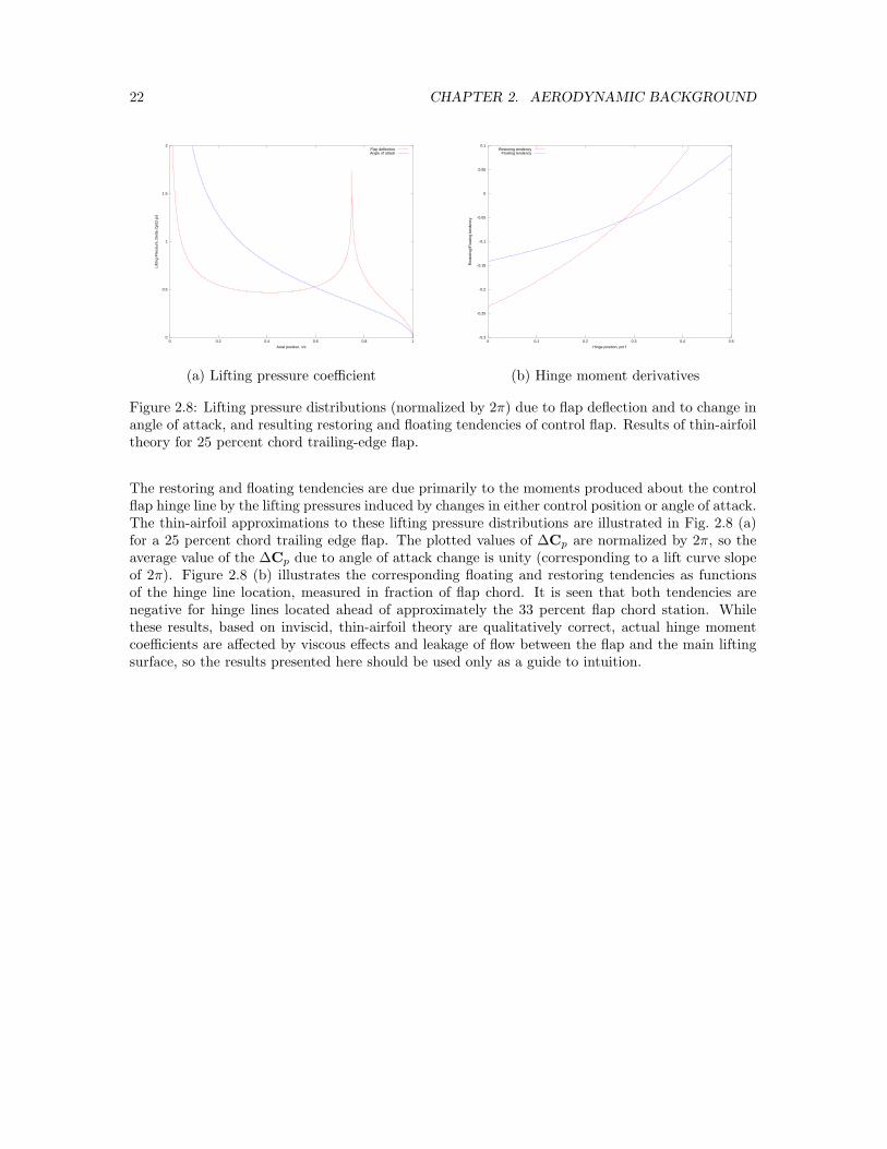
Figure 2.8: Lifting pressure distributions (normalized by 2π) due to flap deflection and to change inangle of attack, and resulting restoring and floating tendencies of control flap. Results of thin-airfoiltheory for 25 percent chord trailing-edge flap.

The restoring and floating tendencies are due primarily to the moments produced about the controlflap hinge line by the lifting pressures induced by changes in either control position or angle of attack.The thin-airfoil approximations to these lifting pressure distributions are illustrated in Fig. 2.8 (a)for a 25 percent chord trailing edge flap. The plotted values of ∆Cp are normalized by 2π, so theaverage value of the ∆Cp due to angle of attack change is unity (corresponding to a lift curve slopeof 2π). Figure 2.8 (b) illustrates the corresponding floating and restoring tendencies as functionsof the hinge line location, measured in fraction of flap chord. It is seen that both tendencies arenegative for hinge lines located ahead of approximately the 33 percent flap chord station. Whilethese results, based on inviscid, thin-airfoil theory are qualitatively correct, actual hinge momentcoefficients are affected by viscous effects and leakage of flow between the flap and the main liftingsurface, so the results presented here should be used only as a guide to intuition.

Bibliography

[1] Ira H. Abbott & Albert E. von Doenhoff, Theory of Wing Sections; Including a Summary

of Data, Dover, New York, 1958.

[2] Holt Ashley & Marten Landahl, Aerodynamics of Wings and Bodies, Addison-Wesley,Reading, Massachusetts, 1965.

[3] Bernard Etkin & Lloyd D. Reid, Dynamics of Flight; Stability and Control, John Wiley& Sons, New York, Third Edition, 1998.

[4] Robert C. Nelson, Flight Stability and Automatic Control, McGraw-Hill, New York,Second Edition, 1998.

[5] Edward Seckel, Stability and Control of Airplanes and Helicopters, Academic Press,New York, 1964.

[6] Richard Shevell, Fundamentals of Flight, Prentice Hall, Englewood Cliffs, New Jersey, Sec-ond Edition, 1989.

23

aerodynamic background - cornell - cornell university · pdf filechapter 2 aerodynamic...

Documents