aep’s 2016 price elasticity study - energy...

AEP’s 2016 Price Elasticity Study

Chad Burnett

Director of Economic Forecasting

April 2017

Energy Forecasting Meeting

Chicago, IL

Who Is AEP?

• AEP is one of the largest electric utilities in the US, serving nearly 5.4 million customers in 11 states

• The largest Transmission network in the US (over 40,000 miles)

• Approximately 26,000 megawatts of generating capacity

• 7 distinct operating companies in 11 states = 15 jurisdictions

AEP Regulated Operating Companies– AEP-Ohio– AEP-Texas– Appalachian Power– Indiana Michigan Power– Kentucky Power– Public Service Co. of Oklahoma– Southwestern Electric Power Co.

2

Who Are Our Customers?

• Household Incomes in AEP service territory are over 18% ($9,709) below the US average.

• In every state except Ohio & Arkansas, AEP service territory incomes are below the state average as well.

• 94% of our customers live in counties where the median household income is below the US average.

3

How Old Is Your Home?

• The majority of AEP customers live in older homes.

• Less than 5% of our customers live in homes that were built within the last 5 years while over 40% of our customers live in homes that are over 40 years old.

• Over half of our customers in I&M and AEP-Ohio live in homes that are over 40 years old.

Source: AEP’s 2016 Residential Appliance Saturation Survey (RASS)

4

Recent Turnover in Appliance Stock

• Despite the age of our customer’s homes, it appears many of the major end-use appliances have been replaced within the last 5 years.

• Typically, newer appliances are more energy efficient than the older units they replaced.

Source: AEP’s 2016 Residential Appliance Saturation Survey (RASS)

5

How Do You Heat Your Home?

• 46% of our customers use electricity to heat their homes.• The highest saturation of electric heating is in South Texas (83%).

However, because of relatively warmer winter temperatures and smaller home sizes, the heating load for TCC is not as much as other AEP operating companies.

• APCo and KPCo also have relatively high saturations of electric heating (> 60%) due to the unavailability of alternative fuel sources. The natural gas distribution system is less developed in the mountainous terrain of the Appalachian territory.

Source: AEP’s 2016 Residential Appliance Saturation Survey (RASS)6

Change in Historical Usage Trend

• Prior to 2005, the growth in normalized usage for the Residential and Commercial sectors was fairly steady and consistent.

• Since 2005, the trend has changed and usage has started to decline.• This study is designed to help explain what is causing the change.

7

Residential Price Elasticity Study

8

Relationship Between Price and Usage

• The law of demand states that as price increases, the quantity demanded will decrease.

• Price elasticity measures how responsive customers are to changes in price. • Elasticities are typically lower in the short run (within 1st year) than the long

run since customers have more substitution options (i.e. more efficient appliances) over time.

• The demand for electricity is still relatively inelastic, although our study may indicate customers are becoming more responsive to price changes than they were historically.

9

Previous Studies Results

• There have been a number of studies done on a national level over the past 40+ years which have estimated the long run electric price elasticity for the residential sector to be around |0.2 - .8|.

• Two studies- RAND (2005) and Paul (2009) estimated regional elasticities and discovered the regions where AEP is located (East North Central and West South Central) were generally less elastic than the US. This could be explained by the lack of available substitutes (natural gas) as indicated in the Residential Appliance Saturation Survey results.

• In 2009, AEP’s Economic Forecasting group performed its own study and estimated AEP’s Residential electric price elasticity to go from -0.05 in the short term to -0.16 in the long term.

• An elasticity value of -0.16 means if an operating company raised its price by 10%, its Residential sales would decrease by 1.6%, assuming nothing else changes.

10

External Electricity Price Elasticity Research

Study Short Run Long Run

Taylor (1975) Range from -.9 to -.13 Range from -2.0 to 0

Bohi and Zimmerman (1984) -0.20 -0.70

Maddalla et al. (1997) -0.16 -0.24

Rand - Bernstien and Griffin (2005) -0.24 -0.32

Paul, et. al (2009) -0.13 -0.40

Alberini, et. al (2011) -0.15 -0.78

Average (excluding Taylor) -0.18 -0.49

Region Short Run (Rand Study, 2005) Short Run (Paul, et al 2009)

West South Central -0.13 -0.11

East North Central -0.05 -0.12

Region Long Run (Rand Study, 2005) Long Run (Paul, et al 2009)



National Level Estimates

Regional Estimates

Residential Price Elasticity Model

• For the 2016 Elasticity study, we started with the same modeling approach as the 2009 study and the RAND (2005) study- Two Way Fixed Effects Model using a pooled dataset starting in 1992.

• One major enhancement to the 2016 study was the addition of an energy efficiency index (based on SAE efficiency inputs) to isolate the impact that EE is having on Residential sales independent of the impact of price increases, etc.

• The model was also re-estimated using data only through 2005 and 2010, respectively, to test if customers have become more responsive to price increases over time.

Sales = f(Lagged Sales, Electricity Price, Natural Gas Price,

Income, Population, Degree Days, Energy Efficiency)

11

Energy Efficiency Index

• The Energy Efficiency Index was derived from Itron’s SAE model inputs for each operating company.

• The various Commissions have taken different regulatory positions to promote (or mandate) higher saturations of energy efficient technologies over the past decade. This helps explain the variation in the EE index across operating companies.

12

Residential Elasticity Study Results

• The EE Index variable was statistically significant and helps explain the change in Residential sales growth.

• The test confirms that customers are becoming more price responsive over time.

• The model estimated the short-run elasticity (within 1 year) of -0.08 and the long-run elasticity of -0.14.

13

Coefficient P-Value

Long Term

Elasticity

Lag Sales 0.44 <.0001

Electric Price -0.08 <.0001 -0.14

Gas Price 0.05 <.0001 0.05

Income 0.21 <.0001 0.22

Population 0.49 0.001 0.63

Degree Days 0.32 <.0001 0.64

EE -0.24 <.0001 -0.35

R2 0.9995

n 360

Two-Way Fixed Effects

Elasticity Results by Jurisdiction

• Elasticities may be different by jurisdiction for a number of reasons (availability of substitutes, incomes, historical price increases, etc.)

• Based on the 2016 study results, customers in deregulated jurisdictions (right of the dashed line) are generally more responsive to price increases than customers in other jurisdictions.

• Directionally, the results of AEP’s 2016 elasticities by jurisdiction correspond fairly well with the regional differences identified in the 2005 RAND study.

14

What Does This Mean?

• The biggest driver of the decline in Residential usage over the past decade was the impact of energy efficiency. Federal policies combined with company sponsored DSM programs helped accelerate the adoption of newer, energy efficient appliances in customer’s homes.

• The impact of increasing electricity prices (26% faster than inflation between 2005 and 2015), also significantly impacted Residential usage growth over the past 10 years.

• Fortunately, real household incomes have increased 15% since 2005 to help offset the drag from prices and energy efficiency.

15

Commercial Price Elasticity Study

16

Published Research for Commercial Elasticities

• The Commercial class is less homogenous than the Residential sector (i.e. gas stations, restaurants, hospitals, universities, etc.) which makes the modeling slightly different (i.e. more challenging).

• As you might expect, research shows Commercial class to be marginally more price responsive than Residential sector.

External Price Elasticity Research


Bohi and Zimmerman (1984) 0.00 -0.26

Rand - Bernstien and Griffin (2005) -0.21 -0.97

Paul, et. al (2009) -0.11 -0.29

Average -0.11 -0.51

Region Short Run (Rand Study) Short Run (Paul, et al 2009)



Region Long Run (Rand Study) Long Run (Paul, et al 2009)



National Level Commercial Estimates

Regional Estimates

17

Commercial Price Elasticity Model

• For the Commercial model, we started with the same modeling approach as the RAND (2005) study- Two Way Fixed Effects Model using pooled data.

• Similar to Residential, we added an energy efficiency index variable to isolate the impact that EE is having on Commercial sales separate from the impact of price increases, etc.

• The model was also re-estimated using data only through 2010, to test if customers have become more responsive to price increases over time.

• We also tested a Rational Expectations approach using projected electric Prices, natural gas prices, and commercial GDP (+3 years and +6 years) and came up with similar results.


Commercial GDP, Population, Degree Days, Energy Efficiency)

18

Commercial Elasticity Study Results

• The EE Index variable was statistically significant and helps explain the change in Commercial sales growth.

• The model estimated the short-run elasticity (within 1 year) of -0.10 and the long-run elasticity of -0.27.

• The study also confirms that Commercial customers are more price responsive than Residential customers.

19

Coefficient P-Value

Long Term

Elasticity

Lag Sales 0.64 0.000

Electric Price -0.10 0.000 -0.27

Gas Price 0.03 0.000 0.10

ComGDP 0.10 0.000 0.27

Population 0.17 0.073 0.46

Degree Days 0.14 0.000 0.39

EE -0.07 0.003 -0.18

MACSS 0.09 0.000 0.24

R2 0.9992

n 360



• Unlike Residential, the biggest drag on Commercial usage over the past decade is the result of electric price increases (12% faster than inflation).

• The decline in usage attributed to Energy Efficiency gains was also significant over the test period as various energy policies (both Federal and State) along with company sponsored DSM programs have targeted several Commercial end-uses.

• The significant drop in natural gas prices (and corresponding increase in electric prices) resulted in some customers investing in substitute technologies.

• Fortunately, the increase in Commercial GDP and Population (Economy) is helping to offset the drag from electric prices, energy efficiency, and natural gas prices. 20

Industrial Price Elasticity Study

21

Industrials Making More With Less

• Over the past several decades, US Manufacturing has become much more efficient (i.e. producing more with less).

• Industrial Production (Output) has increased over 62% since 1990 with only a 4% increase in electricity usage and a 30% reduction in employment.

22

Published Research for Industrial Elasticities

• The Industrial class is even less homogenous than the Residential and Commercial sectors which makes the modeling even more challenging.

• Fewer studies on Industrial elasticities have been published (especially at the regional level) and the research that does exist shows a wide range of long term elasticities |0.4 – 3.3|.

• You would expect Industrial customers to be more price responsive than Residential and Commercial customers.

• In the one study that performed regional analysis (Paul), the elasticity estimates for the regions covering AEP’s service territory were typically lower than the US as described in the Residential and Commercial sections.

23

External Price Elasticity Research


Taylor (1977) -0.22 -1.63

Bohi and Zimmerman (1984) -0.11 -3.26

Dahl and Roman (2004) -0.14 -0.56

Paul, et. al (2009) -0.16 -0.40

Garen, et. al (2011) -0.22 -0.83

Average -0.17 -1.34

Region Short Run (Paul, et al 2009) Long Run (Paul, et al 2009)



National Level Commercial Estimates

Regional Estimates

Industrial Price Elasticity Model

• For the Industrial model, we started with the same modeling approach as the Residential and Commercial models- Two Way Fixed Effects Model using pooled data by industrial classification.

• We recognize that there are multiple aspects of efficiency occurring in the Industrial class: Employment Efficiency (more output using fewer employees) as well as Technological Efficiency (more output using more energy efficient processes). To address this, we introduced an Electric Intensity variable (Industrial GDP/MWh) in the model.

• The Company’s records of industrial data by NAICS did not go back as far as Residential and Commercial classes, so we were unable to test how these elasticity estimates have changed over time.


Employment (by Industry), Electric Intensity)

24

Industrial Elasticity Study Results

• The Intensity variable was statistically significant and helps explain the change in Industrial sales growth.

• Natural gas prices were not statistically significant but were left in the model based on economic theory.

• The model estimated the short-run elasticity (within 1 year) of -0.23 and the long-run elasticity of -1.26, which would not be classified as inelastic.

• The study also confirms that Industrial customers are more price sensitive than Residential and Commercial customers.

25

Coefficient P-Value

Long

Term

Elasticity

Lag Sales 0.81 0.000

Electric Price -0.23 0.025 -1.26

Gas Price 0.05 0.723 0.28

Employment 0.12 0.001 0.67

Intensity -0.11 0.003 -0.59

R2 0.9887

n 120


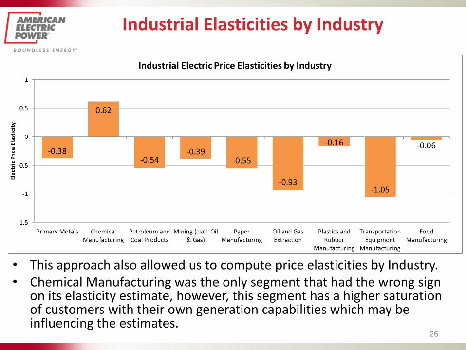
Industrial Elasticities by Industry

• This approach also allowed us to compute price elasticities by Industry. • Chemical Manufacturing was the only segment that had the wrong sign

on its elasticity estimate, however, this segment has a higher saturation of customers with their own generation capabilities which may be influencing the estimates.

26


• The biggest driver behind the drop in Industrial sales was the impact of price increases (22% faster than inflation over the past decade). This is not surprising given the elastic demand of Industrial customers.

• The significant drop in natural gas prices (-50%) and corresponding increase in electric prices resulted in some customers investing in substitute technologies.

• ‘Efficiency investments’ in newer technologies/processes that require fewer employees and less electricity are also creating a drag on Industrial sales growth.

• Fortunately, Economic Development and the addition of new customer loads (shale gas revolution) are helping to offset the drag from higher electricity prices, lower natural gas prices, and more efficient processes from Manufacturing firms.

27

Questions?

28

aep’s 2016 price elasticity study - energy...

Documents