aea 505: econometrics department of agricultural …

i

NATIONAL OPEN UNIVERSITY OF NIGERIA

AEA 505: ECONOMETRICS

DEPARTMENT OF AGRICULTURAL ECONOMICS AND EXTENSION

FACULTY OF AGRICULTURAL SCIENCES

NATIONAL OPEN UNIVERSITY OF NIGERIA

ii

COURSE DEVELOPER: DR. M. A. OTITOJU

DEPARTMENT OF AGRICULTURAL ECONOMICS

UNIVERSITY OF ABUJA

ABUJA, NIGERIA

COURSE GUIDE

CONTENTS

Introduction --- - - - -- -- - -- -- iii

What you will learn in this course --- -- -- -- -- -- -- iii

Course aim -- -- -- -- -- -- -- -- -- -- iii

Course objectives -- -- -- -- -- -- -- -- -- iii

Working through this course -- -- -- -- -- -- -- iv

Course materials -- -- -- -- -- -- -- -- iv

Study units -- -- -- -- -- -- -- -- -- iv

Textbooks and references -- -- -- -- -- -- -- -- vii

Assignment file -- -- -- -- -- -- -- -- vii

Tutor-marked assignment -- -- -- -- -- -- -- vii

Facilitators/tutors and tutorials -- -- -- -- -- -- -- viii

Summary -- -- -- -- -- -- -- -- -- viii

iii

INTRODUCTION

AEA 505 Econometrics is a two-credit unit course. The course consist of 20 units covering the definition and

scope of econometrics, methodology of econometrics, types and importance of econometrics, regression

analysis, parameter estimates using ordinary least square method, correlation analysis, problems in regression

analysis and analysis of variance. This course guide gives you insight into the nature of the course materials you

are going to use and how you are to use the materials for meaningful benefits.

You are encouraged to devote, at least, four hours to study each of the 20 units. You are also advised to to pay

more attention to the tutor-marked assignment.

This Course Guide is meant to provide you with the necessary information about the methodology of

econometrics, regression analysis, correlation analysis and analysis of variance and provide policy

interpretations. The course demonstrate the nature of the materials you will be using and how to make the best

use of the materials towards ensuring adequate success in your programme as well as the practice of economic

policy analysis. Also included in this course guide are information on how to make use of your time and

information on how to tackle the tutor-marked assignment (TMA) questions. There will be tutorial sessions

during which your instructional facilitator will take you through your difficult areas and at the same time have

meaningful interaction with your fellow learners.

WHAT YOU WILL LEARN IN THIS COURSE

Econometrics provides you with the opportunity to gain mastery and an in-depth understanding of the basic

econometrics in agriculture.

COURSE AIM

The aim of this course is to give better understanding of to the major aspects of econometrics. This begins with

knowing the meaning of econometrics, methodology of econometrics, types and importance of econometrics,

regression analysis, parameter estimates using ordinary least square method, correlation analysis, problems in

regression analysis and analysis of variance.

COURSE OBJECTIVES

In order to achieve the aim of this course, there are sets of overall objectives. Each unit also has specific

objectives. The unit objectives are always included in the beginning of the unit. You need to read them before

iv

you start working through the unit. You may also need to refer to them during your study of the unit to check

your progress. You should always look at the unit objectives after completing a unit.

Below are the wider objectives of the course as a whole. By meeting these objectives you should have achieve

the aims of the course as a whole. On successful completion of the course, you should be able to:

define econometrics

describe the traditional classical methodology of econometrics research

state and explain the types and importance of econometrics

state and explain types of variables

define regression analysis and explain types of regression analysis

explain non-linear regression analysis

describe various types of data for regression analysis

explain the techniques for estimating parameters of regression models and assumptions

on Ordinary Least Square (OLS) Estimates

discuss the causes of deviation of observation from the fitted line

explain how to use the Ordinary Least Squares Method (OLS) to estimate regression parameters

formulate and test hypothesis using various tools

explain the meaning of correlation

describe types/forms of correlation

explain the procedures for computing correlation coefficient

test the significance of correlation coefficient

describe the limitations of linear correlation

differentiate between correlation and regression

explain the problems in regression analysis

describe the meaning and essence of analysis of variance

state and explain the various types of analysis of variance

v

explain the various approaches to analysis of variance

interpretation the Analysis of Variance Results

WORKING THROUGH THIS COURSE

To complete this course you are required to read the study units, read suggested books and other materials that

will help you achieve the stated objectives. Each unit contains Tutor Marked Assignment (TMA) and at

intervals as you progress in the course, you are required to submit assignment for assessment purpose. There

will be a final examination at the end of the course.

During the first reading, you are expected to spend a minimum of two hours on each unit of this course. Below

you will find listed components of the course, what you have to do and how you should allocate your time.

Discussion group of between three to five people will be ideal.

COURSE MATERIALS

The major components of the course include the following:

1. Course guide

2. Study units

3. Textbooks and references

4. Assignment file

STUDY UNITS

There are 20 study units in this course as follows:

Module 1 Introduction to Econometrics

Unit 1 Definition and Scope of Econometrics

Unit 2 Methodology of Econometrics

Unit 3 Types and importance of Econometrics

Module 2 Regression Analysis

Unit 1 Definition and types of Variables

Unit 2 Meaning and types of Regression Analysis

vi

Unit 3 Non-linear Regression Analysis

Unit 4 Data for Regression Analysis

Module 3 Parameter Estimates Using Ordinary Least Square (OLS) Method

Unit 1 Techniques for Estimating Parameters of Regression Models and Assumptions

on Ordinary Least Square (OLS) Estimates

Unit 2 Causes of Deviation of Observation from the fitted line

Unit 3 The Ordinary Least Squares Method (OLS)

Unit 4 Parameter Testing (Hypothesis formulation and Testing)

Module 4 Correlation Analysis

Unit 1 The meaning of Correlation

Unit 2 Types/forms of Correlation

Unit 3 Procedures for Computing Correlation Coefficient

Unit 4 Test of Significance of Correlation Coefficient

Unit 5 Limitations of Linear Correlation and Correlation versus Regression

Module 5 Problems in Regression Analysis

Unit 1 Explaining the problems in regression analysis

Unit 2 Autocorrelation

Unit 3 Multicollinearity

Unit 4 Heteroscedasticity

Module 6 Analysis of Variance (ANOVA)

Unit 1 The Meaning and Essence of Analysis of Variance (ANOVA)

Unit 2 Types of Analysis of Variance (ANOVA)

Unit 3 Approaches to Analysis of Variance (ANOVA)

Unit 4 Interpretation of Analysis of Variance (ANOVA) Results

TEXTBOOKS AND REFERENCES

Aiyedun, E. A. (1998). Applied Econometrics, Enidun Ventures Limited, Abuja.

Awoke, M. U. (2002). Econometrics: theory and Application. Willy & Appleseed Publishing

Coy, Abakaliki, Nigeria.

Cameron, A. C. & Trivedi, P. K. (2005). Microeconometrics: Methods and Applications.

Cambridge University Press, Cambridge, UK.

Gujarati, D.N., Porter, D. C. & Gunasekar, S. (2012). Basic Econometrics 5th

Edition, Tata

McGraw Hill Educational Private Limited, New Delhi, India.

Osuala, A. E. (2010). Econometrics: Theory and Problems. ToniPrints Services, Abia State,

Nigeria.

Wooldridge, J. M. (2013). Introductory Econometrics: A Modern Approach, 5th

Edition, South-

Western Centage Learning, Mason, USA.

ASSIGNMENT FILE

In the assignment file, you will find the details of the assignment you must submit to your tutor

for making. There are many assignments on this course and you are expected to do all of them by

following the schedule prescribed for them in terms of when to attempt them and submit same

for grading by your tutor. The marks you obtain for these assignments will count towards the

final score.

TUTOR-MARKED ASSIGNMENT

The Tutor-Marked Assignment TMA is the continuous assignment component of this course. It

account for 30 percent of the total score. You will be given about six TMAs to answer. At least

four of them must be answered from where the facilitator will pick the best three for you. You

must submit all your TMAs before you are allowed to sit for the end of course examination. The

TMAs would be given to you by your facilitator and return to him or her after you have done the

assignments.

FINAL EXAMINATION AND GRADING

This examination concludes the assessment for the course. It constitutes 70 percent of the whole

course. You will be informed of the time for the examination through your study centre manager.

FACILITATORS/TUTORS AND TUTORIALS

There are 20 hours of tutorials provided in support of this course. You will be notified of the

dates, times and location of these tutorials, together with the names and phone number of your

tutor, as soon as you are allocated a tutorial group.

Your tutor will mark and comment on your assignments; keep a close watch on your progress

and on any difficulties you may encounter as this will be of help to you during the course. You

must mail your tutor-marked assignments to your tutor-well before the due date (at least two

working days are required). They will be marked by your tutor and returned to you as soon as

possible.

Do not hesitate to contact your tutor by telephone, e-mail, or discussion board if you need help.

The following may be circumstances in which you would find help necessary. Contact your tutor

if:

you do not understand any part of the study units or the assigned readings.

you have question(s) or problem(s) with tutor‟s comments on any assignment or with the

grading of an assignment.

you should try your best to attend tutorials. This is the only chance to have face-to-face

contact with your tutor and to ask question which are course of your study. To gain

maximum benefit from course tutorials, prepare your list of questions ahead of time. You

will learn a lot from participating in the discussions.

SUMMARY

AEA 505: Econometrics is a course that gives the basic understanding of econometrics and

explains the basics. It covers the definition and scope of econometrics, methodology of

econometrics, types and importance of econometrics, regression analysis, parameter estimates

using ordinary least square method, correlation analysis, problems in regression analysis and

analysis of variance.

We wish you success and hope that you will find the course interesting and useful. Good luck!

TABLE OF CONTENTS

MODULE 1: INTRODUCTION TO ECONOMETRICS -- -- -- 1

Unit 1: Definition and Scope of Econometrics -- --- --- --- --- --- 1

Unit 2: Methodology of Econometrics -- -- --- -- -- -- -- 7

Unit 3: Types and importance of Econometrics-- -- -- -- -- 14

Unit 4: -- -- -- -- -- 19

MODULE 2: REGRESSION ANALYSIS -- -- -- -- -- 19

Unit 1 Definition and types of Variables -- -- -- -- -- -- 19

Unit 2 Meaning and types of Regression Analysis -- -- -- 24

Unit 3 Non-linear Regression Analysis -- -- -- -- -- 31

Unit 4 Data for Regression Analysis -- -- -- -- -- -- 37

MODULE 3: PARAMETER ESTIMATES USING ORDINARY

LEAST SQUARE (OLS) METHOD -- -- -- -- -- -- -- 45

Unit 1: Techniques for Estimating Parameters of Regression Models and

Assumptions on Ordinary Least Square (OLS) Estimates -- --- 45

Unit 2: Causes of Deviation of Observation from the fitted line --- -- 53

Unit 3: The Ordinary Least Squares Method (OLS)-- -- -- -- -- 61

Unit 4: Parameter Testing (Hypothesis formulation and Testing) --- -- 77

MODULE 4: CORRELATION ANALYSIS -- -- -- -- -- 89

Unit 1: The meaning of Correlation -- -- -- -- -- -- 89

Unit 2: Types/forms of Correlation -- -- -- -- -- -- 93

Unit 3: Procedures for Computing Correlation Coefficient -- -- -- 99

Unit 4: Test of Significance of Correlation Coefficient -- -- -- 112

Unit 5: Limitations of Linear Correlation and Correlation

versus Regression -- -- --- --- -- --- -- -- 119

MODULE 5: PROBLEMS IN REGRESSION ANALYSIS -- -- -- 123

Unit 1: Explaining the problems in regression analysis -- -- -- 123

Unit 2: Autocorrelation -- --- -- -- -- - -- -- 126

Unit 3: Multicollinearity -- -- -- -- -- -- -- -- 134

Unit 4: Heteroscedasticity -- --- -- -- -- -- -- -- 144

MODULE 6: ANALYSIS OF VARIANCE (ANOVA) -- -- -- 152

Unit 1: The Meaning and Essence of Analysis of

Variance (ANOVA) -- -- -- -- -- -- -- 152

Unit 2: Types of Analysis of Variance (ANOVA) -- -- -- 158

Unit 3: Approaches to Analysis of Variance (ANOVA) -- -- -- 166

Unit 4: Interpretation of Analysis of Variance (ANOVA) Results -- -- 186

1

MODULE 1: INTRODUCTION TO ECONOMETRICS

Unit 1: Definition and Scope of Econometrics

Unit 2: Methodology of Econometrics

Unit 3: Types and importance of Econometrics

Unit 4:

UNIT 1: DEFINITION AND SCOPE OF ECONOMETRICS

CONTENTS

1.0 Introduction

2.0 Objectives

3.0 Main content

3.1 Definition and scope of Econometrics

3.2 Why is Econometrics a Separate Discipline

4.0 Conclusion

5.0 Summary

6.0 Tutor-Marked Assignment

7.0 References/Further Readings

1.0 INTRODUCION

The study of econometrics has become an essential part of every undergraduate

course in agricultural economics, and it is not an exaggeration to say that it is also

an essential part of every economist‟s training. This is because the importance of

applied economics is constantly increasing and the ability to quantify and evaluate

economic theories and hypotheses constitutes now, more than ever, a bare

necessity. Theoretical economics may suggest that there is a relationship between

two or more variables, but applied economics demands both evidence-based

2

relationship of real life situation and quantification of this relationship using actual

data. This is known as econometrics.

2.0 OBJECTIVES

At the end of this unit, you should be able to:

understand the basic fundamentals of Econometrics

distinguish between economic theory, mathematical economics, economic

statistics and econometrics.

3.0 MAIN CONTENT

3.1 Definition and Scope of Econometrics

Econometrics literally means economic measurement: “econo-metrics”.

Econometrics is the application of statistical methods to the study of economic

data and problems.

Econometrics is the branch of economics concerned with the use of mathematical

methods especially statistics in describing economic systems.

Econometrics is a branch of science that is concerned with the integration of

economics, mathematics, statistics for the purpose of measuring and testing

economic phenomena or relationships.

Econometrics could also mean a branch of knowledge, which aims at the

measurement of relationships between economic variables, values and predictions.

Econometrics may be defined as the social science in which the tools of economic

theory, mathematics, and statistical inference are applied to the analysis of

economic phenomena.

Econometrics is concerned with the empirical determination of economic laws.

3

Thus, it is a special type of economic analysis involving the integration of

economics, mathematics and statistics and other related courses or subjects.

The above definitions show that econometrics encompasses three (3) basic

components:

i. economics

ii. mathematical analysis

iii. statistical analysis

aimed at achieving useful targets.

Econometrics is an amalgam of economic theory, mathematical economics,

economic statistics, and mathematical statistics. Yet the subject deserves to be

studied in its own right for the following reasons:

i. Economic theory makes statements or hypotheses that are mostly qualitative

in nature. For example, microeconomic theory states that, ceteris paribus

(i.e. other things remaining the same), a reduction in the price of a

commodity is expected to increase the quantity demanded of that

commodity. Thus, economic theory postulates a negative or inverse

relationship between the price and quantity demanded of a commodity. But

the theory itself does not provide any numerical measure of the relationship

between the two; that is, it does not tell by how much the quantity will go up

or down as a result of a certain change in the price of the commodity. It is

the job of the econometrician to provide such numerical estimates. Stated

differently, econometrics gives empirical content to most economic theory.

ii. Mathematical economics expresses economic theory in mathematical

form or equations (models) without regard to measurability or

empirical verification of the theory. We may, thus, express the above

4

economic theory, the relationship between price and quantity demanded of a

commodity as stated above in equation form as:

Qd = β0 - β1P --- --- --- --- --- (1.1)

Where:

Qd = Quantity demanded of the commodity

P = Price of the commodity

β0 = intercept (constant)

β1 = the slope coefficient.

The above demand equation or model assumes a deterministic or an exact

relationship between the dependent variable (i.e. Qd) and the independent

variable (i.e. P), which means that only price of the commodity (P) can

influence the quantity demanded, Qd. We do know however, that in reality,

there are a host of factors that influence or determine the quantity demanded

of a product apart from price. These factors include: taste, price of other

commodity (close substitute), consumers‟ income, wars, invention of a

product, migration, technological advancements, literacy level, etc.

Econometrics, as noted previously, is mainly interested in the empirical

verification of economic theory. As we shall see, the econometrician often

uses the mathematical equations proposed by the mathematical economist

but puts these equations in such a form that they lend themselves to

empirical testing. And this conversion of mathematical into econometric

equations or models requires a great deal of ingenuity and practical skill.

iii. Economic statistics is mainly concerned with collecting, processing, and

presenting economic data in the form of charts and tables. These are the

jobs of the economic statistician. It is he or she who is primarily responsible

5

for collecting data on gross national product (GNP), employment,

unemployment, prices, etc. The data thus collected constitute the raw data

for econometric work. But the economic statistician does not go any further,

not being concerned with using the collected data to test economic theories.

Of course, one who does that becomes an econometrician. Although

mathematical statistics provides many tools used in the trade, the

econometrician often needs special methods in view of the unique nature of

most economic data, namely, that the data are not generated as the result of a

controlled experiment.

The Scope of Econometrics includes the following:

Developing statistical methods for the estimation of economic relationships,

Testing economic theories and hypotheses,

Evaluating and applying economic policies,

Collecting and analyzing non-experimental or observational data.

Forecasting.

3.0 CONCLUSION

In this unit you have learnt about basic fundamentals of Econometrics; and to

distinguish between economic theory, mathematical economics, economic statistics

and econometrics.

5.0 SUMMARY Therefore at this end I believe you must have understood the meaning and

scope of econometrics.

6.0 TUTOR MARKED ASSIGNMENT i. What do you understand by econometrics?

6

ii. Vividly differentiate Econometrics from economic theory. Mathematical

economics and Economic statistics.

7.0 REFERENCES/FURTHER READINGS

Awoke, M. U. (2002). Econometrics: theory and Application. Willy & Appleseed

Publishing Coy, Abakaliki, Nigeria.


Edition, Tata McGraw Hill Educational Private Limited, New Delhi, India.

Osuala, A. E. (2010). Econometrics: Theory and Problems. ToniPrints Services,

Abia State, Nigeria.

7

UNIT 2 METHODOLOGY OF ECONOMETRICS

CONTENTS

1.0 Introduction

2.0 Objectives

3.0 Main content

3.1 Methodology of Econometrics

4.0 Conclusion

5.0 Summary



i. INTRODUCTION

You have learnt in the previous unit about the meaning of econometrics and to be

able to differentiate between mathematical economics, statistics, economic theory

and econometrics. Another important aspect of econometrics is the methodology of

econometric research. This is what this unit will address.

ii. OBJECTIVES


explain the traditional or classical stages of econometric research.

3.0 MAIN CONTENT

3.1 Methodology of Econometrics

In any econometric analysis, there are stages or steps that are involved. This is

what is referred to as the methodology. Although there are several schools of

8

thought on econometric methodology, we present here the traditional or classical

methodology, which still dominates empirical research in economics, agricultural

economics and other social sciences. Broadly speaking, traditional econometric

methodology is as follow:

1. Statement of theory or hypothesis

2. Specification of the mathematical model of the theory

3. Specification of the statistical or econometric model

4. Obtaining the data

5. Estimation of the parameters of the econometric model

6. Hypothesis testing

7. Forecasting or prediction

8. Using the model for control or policy purposes.

To illustrate these steps, let us consider the microeconomic theory of demand.

1. Statement of theory or hypothesis

This is the first stage of econometric analysis. It entails finding out the economic

theory or hypothesis that the thrust of the work hinges on. For instance,

microeconomic theory states that, ceteris paribus (i.e. other things remaining the

same), a reduction in the price of a commodity is expected to increase the quantity

demanded of that commodity. Thus, economic theory postulates a negative or

inverse relationship between the price and quantity demanded of a commodity.

This is referred as the statement of theory or hypothesis or maintained hypothesis.

The theory therefore forms the basis for defining the dependent and the

independent variables which will be included in the model, and also the a priori

expectations about the sign and size of the parameters of the model.

9

2. Specification of the mathematical model of the theory

The microeconomic theory (law of demand) only indicated the nature of

relationship between the price and the quantity demanded of the commodity but

did not specify the precise form of their functional relationships. For simplicity, a

mathematical economist might suggest the following form of the law of demand:

Qd = β0 - β1P --- --- --- --- --- (1.2)

Where:

Qd = Quantity demanded of the commodity

P = Price of the commodity,

β0 and β1, known as the parameters of the model.

β0 = intercept (constant)

β1 = the slope coefficient.

A model is simply a set of mathematical equations.

In Equation (1.2) the variable appearing on the left side of the equality sign is

called the dependent variable or regressor and the variable on the right side is

called the independent, or explanatory, variable. Thus, in the microeconomic

theory (law of demand), Equation (1.2), Quantity demanded of the commodity (Qd)

is the dependent variable and price of the commodity is the independent or

explanatory variable.

3. Specification of the statistical or econometric model

This stage entails the representation of economic relationships in explicit stochastic

equation form (i.e. by including in the model or equation a stochastic or error term)

such that equation 1.2 is modified to the form:

Qd = β0 - β1P + µ --- --- --- --- --- (1.3)

Where µ is known as the disturbance, or error, term; it is a random (stochastic)

variable that has well defined probabilistic properties. The disturbance term u may

10

well represent all those factors that affect demand of a commodity but are not

taken into account explicitly. Equation (1.3) is an example of an econometric

model.

4. Obtaining the data

The fourth stage involves the collection of statistical observation (data) on

the variables included in the model (i.e. Equation 1.3). In our example above

(Equation 1.3), only two variables were included: Qd, the quantity demanded

of a commodity, P, the price of the commodity.

5. Estimation of the parameters of the econometric model

This stage entails obtaining numerical estimates (values) of the coefficients (β0 and

β1) in the equation 1.3 of the specified demand model by means of appropriate

econometrics techniques using the data obtained. For now, note that the statistical

technique of regression analysis is the main tool used to obtain the estimates. This

gives the model a precise form with appropriate signs of the parameters for easy

analysis. Using the data obtained, the equation or model becomes for example, Qd

= 59.13 – 2.6P. The estimates of β0 and β1 are 59.13 and -2.6 respectively.

6. Hypothesis testing

Hypothesis testing or statistical inference is done to find out whether the estimates

obtained using the stated model are in agreement with a priori expectations (i.e.

expectations of the economic theory that is being tested). For example, from

demand model, the coefficient β1 should be negative.

Assuming from our estimate using the obtained data, we find that β1 is -2.6. But

before we accept this finding as confirmation of microeconomic theory (law of

demand) , we must enquire whether this estimate is sufficiently different from zero

to convince us that this is not a chance occurrence or peculiarity of the particular

data we have used. In conclusion, -2.6 is statistically different from 0. If it is, it

11

may support microeconomic theory. This type of confirmation or refutation of the

economic theories on the basis of sample evidence is based on a branch of

statistical theory known as statistical inference (hypothesis testing).

7. Forecasting or prediction

The forecasting ability of a model is the ability to accurately predict future values

of the dependent variables based on known or expected future value(s) of the

independent or explanatory variable(s). If the chosen model does not disagree or

refute the hypothesis or theory under consideration, we may use it to predict the

future value(s) of the dependent variable, Qd, quantity demanded of the

commodity.

8. Using the model for control or policy purposes.

In the model, Qd = β0 - β1P, the government can manipulate the control variable, P

to produce the desired level of target variable, Qd.

12

Figure 1.1: Stages of Econometric modeling or research

4.0 CONCLUSION

Stages of econometric modeling or analysis are the process of getting on economic

theory, subject it to econometrics model, and then make use of data, estimation,

and hypothesis testing and policy recommendation.

Economic theory

Estimation of econometric model

Mathematical model of the theory

Econometric model of the theory

Data

Hypothesis testing

Forecasting or prediction

Using the model for control or

policy purposes

13

6.0 SUMMARY The unit has discussed attentively the stages of econometrics analysis or anatomy

of econometric modeling from the economic theory, mathematical model of

theory, econometric model of theory, collecting the data, estimation of econometric

model, hypothesis testing, forecasting or prediction and using the model for control

or policy purposes. Therefore at this end I believe you must have understood the

stages of econometrics analysis or econometric modeling.

8.0 TUTOR MARKED ASSIGNMENT

i. Carefully discuss the stages of econometrics analysis.

ii. What is the major difference between a mathematical model and an

econometric model.








14

UNIT 3 TYPES AND IMPORTANCE OF ECONOMETRICS

CONTENTS

1.0 Introduction

2.0 Objectives

3.0 Main content

3.1. Types of Econometrics

3.2. Importance of Econometrics

4.0 Conclusion

5.0 Summary



1.0 INTRODUCTION

You have learnt in the previous unit about the stages of econometric research and

what makes econometrics a different discipline. Another important aspect of

econometrics is the types and importance of econometrics. This is what this unit

will address.

2.0 OBJECTIVES


identify/explain the types of econometrics analysis.

explain the importance of econometrics

15

3.0 MAIN CONTENT

3.1 Types of Econometrics

Econometrics is broadly divided into two categories: theoretical econometrics

and applied econometrics. In each category, one can approach the subject in the

classical or Bayesian tradition.

1. Theoretical econometrics: This involves the development of econometric

techniques and concepts. It is essentially the development of appropriate

methods for measurement of economic relationships. The econometric

methods so developed could be single-equation techniques or

simultaneous-equation techniques.

The single-equation techniques are econometrics methods that are

developed and applied to one relationship at a time.

Conversely, the simultaneous-equation techniques are developed and

applied simultaneously to all the relationships of a model.

In this aspect, econometrics leans heavily on mathematical statistics.

Theoretical econometrics must spell out the assumptions of this method, its

properties and what happens to these properties when one or more of the

assumptions of the method are not fulfilled.

2. Applied Econometrics: This involves the application of econometrics

methods to specific branches of economic theory. Thus, it is the application

of the tools of theoretical econometrics for the analysis of economic

phenomena and forecasting economic behaviours. The core aim of an

applied econometrics is to bring the economic principles or concepts into

reality through modeling and quantitative forms.

In applied econometrics, we use the tools of theoretical econometrics to

study some special field(s) of economics and business, such as the

16

production function, investment function, demand and supply functions,

portfolio theory etc.

3.2 Importance of Econometrics

The importance of econometrics as an analytical tool or otherwise cannot be over

emphasized. For instance, econometrics has a great application in the areas of

analysis, policy-making and forecasting. These areas (analysis, policy-making and

forecasting) are all inevitable for the sustainable development of any economic

endeavour such as agriculture, manufacturing, commerce, and government

agencies.

i. Analysis: Econometrics helps analysts to test the reliability of economic

theories and hypotheses, and their compatibility with real economic life.

This is done by verifying economic theories and hypotheses from empirical

information. Today, any theory, regardless of its elegance in exposition or its

sound logical consistency, cannot be established and generally accepted

without some empirical testing. Econometrics aids this empirical testing of

theories.

ii. Policy-making: For effective and efficient development in any economic

endeavour, sound decisions need to be made and implemented. This can

only be achieved when effects of alternative policy decisions are compared.

To make this comparison, therefore the knowledge of the numerical values

of coefficients of the economic relationship is very important. These

numerical values can be got through the use of suitable econometrics

techniques. For instance, the production of crops requires the proper

combination of the four factors of production (land, labour, capital and

management). These factors in one way or the other have an influence on the

17

output (yield) of crops. The application of suitable econometrics tools, in the

analysis of the production empirical data will unveil the degree to which

each of these factors influence the output of the production process.

Based on this, farm managers and other decision-makers can decide the fate

of their production on time.

iii. Forecasting: Taking decision in any economic endeavour requires both

short-term and long-term considerations. In the short-term decision-making

may be based on the present observations of economic relationships and its

effects.

Conversely, long-term decision-making process requires making policies

into the future based on present economic situations. This enables process

the policy-makers to judge whether it is necessary to take any measure in

order to influence the relevant economic variables. Econometric models

have been useful in this area. Once models are estimated, they can yield

prediction of future values of endogenous variables. This is conditioned

upon values of exogenous variables supplied.

4.0 CONCLUSION

The different types of econometrics have been discussed; modeling or analysis is

the process of subjecting an economic theory to econometric model, through

estimation of data collected to test hypothesis and make policy recommendation.

5.0 SUMMARY The unit has discussed attentively the type of econometrics. Therefore at this end I

believe you must have understood the types or branches of econometrics.

18


1. Theoretical econometrics differs from applied econometrics. Discuss.

2. What importance or relevance does econometrics have to a socio-economic

research








19

MODULE 2 REGRESSION ANALYSIS

Unit 1 Definition and types of Variables

Unit 2 Meaning and types of Regression Analysis

Unit 3 Data for Regression Analysis

Unit 4 Nonlinear Regression Analysis

UNIT 1 DEFINITION AND TYPES OF VARIABLES

CONTENTS 1.0 Introduction

2.0 Objectives

3.0 Main content

3.1. Meaning and types of variables

4.0 Conclusion

5.0 Summary



1.0 INTRODUCTION

In this unit, you learn the meaning and types of variables in econometrics.

2.0 OBJECTIVES

At the end of this unit, you should be to:

meaning of variables in econometrics

different types of variables

20

3.0 MAIN CONTENT

3.1. Meaning and types of variables

A variable can be continuous or categorical.

1. Continuous variables: These are those variables whose different values are

expressed in numbers. They are also known as quantitative variables.

Examples of continuous variables include:

i. a person‟s age (in years),

ii. weight (in kiolgrammes),

iii. distance (in kilometers),

iv. monthly income (in naira),

v. household size (in numbers),

vi. farm size (in hectares),

vii. years of formal education, etc.

2. Categorical variables: These are those variables whose values are

expressed in categories. They are also known as discrete or qualitative

variables. Examples of categorical variables include:

i. colour (red, white, blue and so on),

ii. food type (maize, millet, rice and so on)

iii. occupation (trader, farmer, artisan).

iv. gender (male or female)

v. marital status (married, single, divorced, widowed).

The categories are often assigned numerical values used as labels, e.g., 0 = male; 1

= female.

3. Dummy variables

These are variables that can take on only the values 0 and 1. They are also known

as binary variables. For example, when a researcher asked whether or not each

21

interviewed respondent belongs to a farmers‟ cooperative society, receives either a

Yes or No answer. These are also in the category of qualitative data.

4. Polychotomous variables

These are variables that can have more than two possible values. They are usually

variables with more than two categories. For example, if a researcher wants to

examine the contribution of women to cocoa production, the contribution can be in

the following categories: high contribution, moderate contribution, and low

contribution. Number can then be assigned to these levels of contribution high

contribution = 1, moderate contribution =2, and low contribution = 3. These are in

more than two categories, hence “poly or multivariate”.

In regression model, variables are in the right hand and the left hand of the model.

The variable on the left hand side of a regression model is called the dependent

variable, or the explained variable, or the response variable, or the predicted

variable, or the regressand.

In equation 1.3 above Qd is the dependent variable. The variable in the right hand

side is referred to the independent variable, or the explanatory variable, or the

control variable, or the predictor variable, or the regressor or the covariate.

In equation 1.3 above, P is the independent variable. The terms „dependent‟

variable and „independent variable‟ are frequently used in econometrics. But be

aware that the label „independent‟ here does not refer to the statistical notion of

independence between random variables.

22

Table 1.1: Types of variables used in Regression analysis

Dependent variable Independent variable

Explained variable Explanatory variable

Response variable Stimulus variable

Predicted variable Predictor variable

Regressand Regressor

Endogenous variable Exogenous variable

Outcome Covariate

Controlled variable Control variable

4.0 CONCLUSION

In this unit you have learnt about meaning and types of variables.

5.0 SUMMARY

In this unit you know that continuous variables are those variables whose different

values are expressed in numbers. They are also known as quantitative variables.

Again, categorical variables are those variables whose values are expressed in

categories. They are also known as discrete or qualitative variables. Dummy or

binary variables are variables that can take on only the values 0 and 1 while

polychotomous variables are variables that can have more than two possible

values. They are usually variables with more than two categories. And in

regression analysis, the variables on the left hand side is referred to as dependent or

endogenous variables, and those on the right hand side is (are) referred to as

independent or explanatory variables.

23

6.0 TUTOR-MARKED ASSIGNMENT

i. What do you understand by continuous and categorical variables?

ii. Differentiate between:

a. Dummy and polychotomous variables

b. Dependent and independent variables.









Edition, South-Western Centage Learning, Mason, USA.

24

UNIT 2 MEANING AND TYPES OF REGRESSION ANALYSIS

CONTENTS

1.0 Introduction

2.0 Objectives

3.0 Main content

3.1. Meaning of Regression Analysis

3.2. Types of Regression Analysis

3.2.1 Simple regression

3.2.2 Multiple regression

3.2.3 Linear regression

3.2.4 Non-linear regression

4.0 Conclusion

5.0 Summary



1.0 INTRODUCTION

You have learnt in the previous unit about the types or branches of econometrics. It

is equally important to address the meaning and type of regression analysis as a

technique used in econometrics. This unit is set to address this.

2.0 OBJECTIVES


explain the meaning of regression analysis in econometrics.

25

understand the types of regression model in econometrics.

differentiate between regression and causation.

3.0 MAIN CONTENT

3.1 Meaning of Regression Analysis

Regression is the most important tool applied economists use to understand the

relationship among two or more variables. As an econometrics tool, it describes in

mathematical form, the relationship between variables. In other words, regression

analysis presents an equation for estimating the amount of change in the value of

one variable associated with a unit change in the value of another variable. In

expressing any relationship in mathematical form, two types of variables can be

identified or involved. Regression analysis is concerned with the study of the

dependence of one variable, the dependent variable, on one or more other

variables, the independent or explanatory variables, with a view to estimating

and/or predicting the (population) mean or average value of the former in terms of

the known or fixed (in repeated sampling) values of the latter.

For example, Y = β0 + β1X + µ. In this regression model, Y is referred to as the

dependent variable, X is the explanatory or independent variable, and β0 and β1

are coefficients. It is common implicitly assume that the explanatory variable X

“causes” the dependent variable Y, and the coefficient β1 measures the influence of

X on Y.

3.2 TYPES OF REGRESSION ANALYSIS

Regression analysis is of different forms. It could be simple, multiple, linear or

non-linear.

26

3.2.1 Simple Regression

This is a regression analysis which describes in mathematical form, the

relationship between two variables. It is also called the two-variable linear

regression model or bivariate linear regression model because it relates two

variables. This implies .that the relationship has one dependent variable and only

one independent variable. Suppose we wish to estimate the parameters of our

reference demand function, stated in the implicit form {Qd = f(P), we can express it

in the explicit form as Qd = β0 - β1P + µ and employ the technique of the simple

regression analysis to estimate its parameter; β0 and β1.

The adoption of the technique of simple regression analysis stems from the fact

that the equation contains only two variables, namely; the dependent variable, Qd

and ONLY ONE independent variable P. The explicit form above implies that

there is a one-way causation between the variables Qd and P. Price, P is the cause

of change in the quantity demanded, but not vice versa. Hence we talk of

regressing quantity demanded of the commodity “Qd” against the price “P”.

Where:

Qd = Quantity demanded of the commodity; P = Price of the commodity; β0 =

intercept (constant); and β1 = the slope coefficient.

When related by demand function or model, Qd = β0 - β1P + µ, the variables Qd and

P have several different names used interchangeably, as follows: Qd is called the

dependent variable, the explained variable, the response variable, the

predicted variable, or the regressand; P is called the independent variable, the

explanatory variable, the control variable, the predictor variable, or the

regressor. (The term covariate is also used for P.) The terms „dependent variable‟

27

and „independent variable‟ are frequently used in econometrics. But be aware that

the label “independent” here does not refer to the statistical notion of independence

between random variables.

The terms “explained” and “explanatory” variables are probably the most

descriptive. “Response” and “control” are used mostly in the experimental

sciences, where the variable P is under the experimenter‟s control. We will not use

the terms “predicted variable” and “predictor,” although you sometimes see these

in applications that are purely about prediction and not causality. Our terminology

for simple regression is summarised in Table 1.1.

The variable u, called the error term or disturbance in the relationship, represents

factors other than P that affect Qd. A simple regression analysis effectively treats

all factors affecting Qd other than P as being unobserved. You can usefully think of

u as standing for “unobserved.”

3.2.2 Multiple Regression analysis

This is an extension of the simple regression analysis. It is a regression that

involves the relationship with more than two variables. Therefore, the multiple

regression analysis is applied to a model with one dependent (explanatory)

variable. Hence, any model with a minimum of two independent variables requires

multiple regression technique for its analysis.

For example, the quantity demanded of any commodity (Qd) depends on such

factors as Price (P) of the commodity, Price (P*) of its close substitute, and

consumer‟s income (Y) among others. The relationship between the quantity

demanded and these factors can be written in its implicit form as:

Qd = f(P, P*, Y).

Explicitly, the above demand function can be written as:

28

Qd = β0 - β1P + β2P* + β3Y + µ

Considering the above equation, it can be seen that Qd is the dependent variable,

while the independent variables are P, P*, and Y. To estimate the parameters (β0,

β1, β2, and β3) of this demand model, we require the application of the multiple

regression analysis (or technique). It is important to note that the number of

independent variables relative to the existing coefficients can be extended to nth

number as the case may be.

3.2.3 Linear Regression

A relationship is linear when it can be described by a linear equation. For

example,

Q = β0 + β1P is a linear function as the plot of its coordinates on a graph will give a

straight line as shown in figure 1.3.

Fig 1.3: Graph of a Linear Equation

In the above illustration, it shows that almost all the points will fall on a straight

line, hence its linear representation.

29

3.2.4 Non-Linear Regression

In this case, a curve rather than a straight line can best describe the relationship.

Example of this type is the Cobb-Douglas production function which has the form,

embracing the dependent variable Q and independent variables K, L, L*, M with

respective coefficients as contained in the models below,

Q = ALβ1

L* β2

K β3

M β4

Q = Output

L = Land

L* = Labour

K = Capital

M = Management.

4.0 CONCLUSION

You have learnt in this unit the different types of regression models (simple,

multiple, linear and non-linear) in econometrics.

5.0 SUMMARY

You have learnt the following:

Simple regression analysis describes in mathematical form, the relationship

between two variables. It is also called the two-variable linear regression

model or bivariate linear regression model because it relates two variables.

Multiple regression involves the relationship with more than two variables.

Therefore, the multiple regression analysis is applied to a model with one

dependent (explanatory) variable.


30

1. With the aid of econometric equations briefly explain the following types

of regression models:

i. Simple regression

ii. Multiple regression

iii. Linear regression

iv. Non-linear regression

2. With the aid of graph differentiate between linear and non-linear

regression models.










31

UNIT 3 NONLINEAR REGRESSION ANALYSIS

CONTENTS

1.0 Introduction

2.0 Objectives

3.0 Main content

3.1. Meaning of Nonlinear Regression

4.0 Conclusion

5.0 Summary



1.0 INTRODUCTION

You have learnt in the previous unit about the types of regression models in

econometrics. It is equally important to address in detail the meaning of non-linear

regression analysis as also a technique used in econometrics. This unit is set to

address this.

2.0 OBJECTIVES


explain the meaning of non-linear regression analysis in econometrics.

3.0 MAIN CONTENT

3.1 Meaning of Nonlinear Regression Analysis

Multiple regression deals with models that are linear in the parameters. That is, the multiple

regression model may be thought of as a weighted average of the independent variables. A linear

32

model is usually a good first approximation, but occasionally, you will require the ability to use

more complex, nonlinear, models.

The meaning of linear

The term linear can be interpreted in two different ways. That is linear in variables and

linear in parameters.

Linearity in the variables: A function or model Y = f (X) is said to be linear in X if X

appears with a power or index of 1 only (that is, terms such as X2, X , and so on, are

excluded) and is not multiplied or divided by any other variable (for example, X.Z or X/Z,

where Z is another variable). If Y depends on X alone, another way to state that Y is

linearly related to X is that the rate of change of Y with respect to X (i.e., the slope, or

derivative, of Y with respect to X, dY/dX) is independent of the value of X.

Thus, if Y = 4X, dY/dX = 4, which is independent of the value of X. But if Y = 4X2, dY/dX

= 8X, which is not independent of the value taken by X. Hence this function is not linear

in X.

Linearity in the parameters: A function is said to be linear in the parameter, say, β0, if

β0 appears with a power of 1 only and is not multiplied or divided by any other parameter

(for example, β1 β2, β1/β2,, and so on).

Linear regression will always mean a regression that is linear in the parameters; the β‟s

(that is, the parameters are raised to the first power only). It may or may not be linear in

the explanatory variables, the X‟s. Schematically, we have Table 2.1.

Table 2.1: Linear Regression Models

Model linear in parameters? Model linear in variables?

Yes No

Yes Linear Regression

Model

Linear Regression Model

No Non-Linear Regression

Model

Non-Linear Regression

Model

33

Then, nonlinear regression models can then be described as those models that are not

linear in the parameters. Examples of nonlinear equations are:

i. exp( )Y a b cX i.e. cXY a b

ii. ( ) / (1 )Y a bX cX

iii. / ( )Y a b c X

iv. by ax

v. bxy a

vi. by a

x

vii. 2

0 1 2Y X X

viii. 2 3

0 1 2 2Y X X X

ix. 0 1X

Y e

To differentiate between linear regression and non-linear regression, table 2.2 below may

be of help. Models a, b, c, and e are linear regression models because they are all linear

in the parameters. Model d is a mixed bag, for β1 is linear but not ln β0. But if we let α =

ln β0, then this model is linear in α and β1. Even models

34

Table 2.2: Types of regression models

Model Descriptive title

a. 10 1 ii iX

Y Reciprocal

b. 0 1 lni i iY X Semilogarithimic

c. 0 1ln i i iY X Inverse semilogarithmic

d. 0 1ln ln lni i iY X Logarithimic or double

logarithmic

e. 10 1ln

ii iXY Logarithmic reciprocal

f. 2

0 1 2Y X X Quadratic

g. 2 3

0 1 2 2Y X X X Cubic

h. 1 1

0

XY e Exponential

However, one has to be careful here, for some models may look nonlinear in the

parameters but are inherently or intrinsically linear because with suitable transformation

they can be made linear-in-the-parameter regression models. But if such models cannot

be linearized in the parameters, they are called intrinsically nonlinear regression

models. From now on when we talk about a nonlinear regression model, we mean that it

is intrinsically nonlinear.

Some standard transformations:

Function Transformation Linear function

expy a bx (i.e. bxy a ) * lny y * lny a bx

by ax * logy y , * logx x * logy a bx

by ax

* 1xx

*y a bx

35

4.0 CONCLUSION

You have learnt in detail the meaning of linear and non-linear regression analysis

as also a technique used in econometrics. This unit addressed the two of linearity,

that is, linearity in the variables and the linearity in the parameters. And how

basically a non-linear models can be transformed to be linear.

5.0 SUMMARY

A function or model Y = f (X) is said to be linear in X if X appears with a power or

index of 1 only (that is, terms such as X2, X , and so on, are excluded) and is not

multiplied or divided by any other variable (for example, X.Z or X/Z, where Z is

another variable).

A function is said to be linear in the parameter, say, β0, if β0 appears with a power

of 1 only and is not multiplied or divided by any other parameter (for example, β1

β2, β1/β2,, and so on).


1. Use the following regression models below to answer the following questions

Yi = β1 + β2(1/X1) + µi --- ------ --- --- -- (1)

Yi = β1 + β2lnX1 + µi --- ------ --- --- -- (2)

lnYi = β1 + β2X1 + µi --- ------ --- --- -- (3)

lnYi = lnβ1 + β2lnX1 + µi --- ------ --- ---(4)

lnYi = β1 - β2(1/X1) + µi --- ------ --- --- -- (5)

(i). Give the name of the regression models (1), (2), (3), (4) and (5) above.

(ii). Classify the functional forms above into linear and non-linear regression

models and explain the reason for their linearity and non-linearity. Then

justify how the one(s) that is (are) non-linear can be linearized.

36










37

UNIT 4 DATA FOR REGRESSION ANALYSIS


2.0 Objectives

3.0 Main content

3.1. Data required for the Estimation of Parameters of Regression

3.2 Types of Data for Regression Analysis

4.0 Conclusion

5.0 Summary



1.0 INTRODUCTION

This unit is very important in regression analysis because it gives the direction to

what type of regression model that would be chosen in any econometric research,

if it would be static or dynamic model. This provides a guide to the type of data

used in econometric analysis.

2.0 OBJECTIVES


data required for the estimation of parameters of regression

explain the various types of data required for model estimation

differentiate between cross-section, time series, pooled cross-section and

panel/ longitudinal data

38

MAIN CONTENT:

3.1 Data required for the estimation of parameters can be from two

sources: Primary and Secondary data

Primary Data

These can be generated from experiments and survey conducted by the researcher.

They are usually those collected for the first time and thus are original in nature.

The primary data can be collected using experimental research design

measurements, observations, interviews, questionnaire, memory recalls, letter of

inquiry, and focus group discussions.

Secondary Data

These are those data which have already been collected by some other persons and

have passed through some statistical processes. Hence, they are not original in

nature but “second hand”. These data can be obtained from published or

unpublished sources, such as official publications of the three tiers of government

(Federal, State and Local), official publications of foreign governments and

international organizations like UNO, FAO, UNDP, IFAD, others reports and

publications of trade associations, banks, co-operatives, reports submitted by

research scholars, university publications, educational associations and so on.

3.2 Types of Data for Regression Analysis

The type of data required for model estimation depends on the nature and purpose

of the research. These data among others include:

i. Cross-section data

ii. Time series data

iii. Pooled cross-section data

39

iv. Panel or longitudinal data

i. Cross-Section/ cross-sectional Data

This set of data is taken or collected at a given point in time from individuals,

households, firms, cities, states, countries, or a variety of other units. In this case

there is no time interval rather data is obtained from different respondents at the

same time. For example, household income, consumption and employment

surveys conducted by the National Bureau of Statistics (NBS).

An example of cross-sectional data on wages and characteristics of heads of

rural households Observation

No.

Wage

(thousand

of naira)

Education

(Years of

schooling)

Experience

(years)

Gender

(Female =1)

Marital Status

(Married =1)

1. 20 11 2 1 0

2. 15 12 22 0 1

3. 12 11 3 1 0

4. 11 6 2 1 1

5. 11.3 0 30 0 1

.

.

.

.

.

.

.

.

.

.

.

.

.

.

.

.

.

.

123 4.6 16 13 0 1

124 11.3 0 5 1 1

125 3.5 6 2 0 0

126 10 12 6 0 0


Time series data consists of observations on a variable or several variables over

time. There is chronological ordering in time series data (that is there is time

40

interval). This is taken in series or interval, which could be hourly, daily, weekly,

monthly, quarterly, yearly or any other time interval. The time length between

observations is generally equal. Examples of time series data include stock prices,

money supply, consumer price index, gross domestic product, annual

unemployment rates, and automobile sales figures for some period of time.

A time series data example on minimum wage, and unemployment

taking annually Observation

No.

Year Minimum Wage (thousand of

naira)

Unemployment

1. 1990 2000 11.3

2. 1991 2000 12.5

3. 1992 2000 11.7

4. 1993 2000 14.5

5. 1994 2000 12.3

.

.

.

.

.

.

.

.

.

.

.

.

21 2014 17000 10.1

22 2015 18000 10.2

23 2016 18000 17.5

24 2017 18000 19.5

Another example is if a researcher wishes to estimate the demand model for beef,

he may gather numerical values for the quantity of beef demanded and other

variables say from 1995 to 2010. These numerical values generated within this

time interval (1995 – 2010) constitute the time series data.

41

iii. Pooled cross-section data:

Pooled cross-section data consists of cross-sectional data sets that are observed

in different time periods and combined together. At each time period (e.g.,

year) a different random sample is chosen from population. Individual units are not

the same. For example if we choose a random sample 400 rural households in 1995

and choose another sample in 1998 and combine these cross-sectional data sets we

obtain a pooled cross-section data set. Cross-sectional observations are pooled

together over time.

A pooled Cross-sectional data example of two years housing prices

Observation No. Year Housing Prices

1. 1995 85500

2. 1995 68550

3. 1995 70200

4. 1995 65000

5. 1995 132500

.

.

.

.

.

.

123 1995 243650

124 1998 65000

125 1998 97000

126 1998 46000

.

.

.

.

.

.

.

.

.

505 1998 56000

42

iv. Panel Data (longitudinal data):

This consists of a time series for each cross-sectional member in the data set.

The same cross-sectional units (firms, households, etc.) are followed over time. For

example: wage, education, and employment history for a set of individuals in rural

areas followed over a ten-year period.

Another example: cross-country data set for a 20 year period containing life

expectancy, income inequality, real GDP per capita and other country

characteristics.

A two-year Panel data set on city crime statistics

Observation

No.

City Year Murders Population

1. 1 1990 2 35000

2. 1 1995 22 34000

3. 2 1990 3 78600

4. 2 1995 2 76800

.

.

.

.

.

.

.

.

.

.

.

.

.

.

.

123 61 1990 13 110000

124 61 1995 5 98500

125 62 1990 2 121000

126 62 1995 123500

4.0 CONCLUSION

In this unit you have learnt about the difference between primary and secondary

data; cross-section data, time series data, pooled cross-section data and panel data.

43

5.0 SUMMARY

In this unit you have learnt that primary and secondary data; cross-section data is a

set of data taken or collected at a given point in time from individuals, households,

firms, cities, states, countries, or a variety of other units. Time series data consists

of observations on a variable or several variables over time. There is

chronological ordering in time series data (that is there is time interval).

Pooled cross-section data consists of cross-sectional data sets that are observed in

different time periods and combined together. At each time period (e.g. monthly,

year) a different random sample is chosen from population, while Panel or

longitudinal data consist of a time series for each cross-sectional member in the

data set. The same cross-sectional units (firms, households, etc.) are followed over

time.


1. What do you understand by the following?

i. Cross-section data


iii. Pooled cross-section data

iv. Panel data

2. Differentiate between primary and secondary data.




44



Koop, G. (2000). Analysis of Economic Data. John Willey & Sons Ltd, New York,

USA.





45

MODULE 3: PARAMETER ESTIMATES USING ORDINARY LEAST

SQUARE (OLS) METHOD

Unit 1: Techniques for Estimating Parameters of Regression Models and

Assumptions on Ordinary Least Square (OLS) Estimates

Unit 2: Causes of Deviation of Observation from the fitted line

Unit 3: The Ordinary Least Squares Method (OLS)

Unit 4: Parameter Testing (Hypothesis formulation and Testing)

UNIT 1: TECHNIQUES FOR ESTIMATING PARAMETERS OF

REGRESSION MODELS AND ASSUMPTIONS OF ORDINARY LEAST

SQUARES (OLS)

CONTENTS

1.0 Introduction

2.0 Objectives

3.0 Main content

4.0 Conclusion

5.0 Summary



1.0 INTRODUCTION

This unit is very important in regression analysis because it gives the direction to

techniques used to determine parameter estimates of regression models. The

assumptions of ordinary least squares (OLS) are as well discussed in this unit

46

2.0 OBJECTIVES


techniques for estimating parameter estimates of regression models

assumptions of ordinary least squares (OLS) technique of estimating

parameter estimates in regression models.

iii. MAIN CONTENT

3.1 TECHNIQUES FOR ESTIMATING PARAMETER ESTIMATES OF

REGRESSION MODELS

To estimate the magnitude of the parameters of a regression model or equation,

there are several techniques that can be used. These techniques include:

i. Ordinary Least Square (OLS) Method

ii. Matrix Method

iii. Indirect Least Square (ILS) Method

iv. Two-Stage Least Square (2SLS)

v. Limited Information Maximum Likelihood (LIML).

Among the above methods, the ordinary least square (OLS) method shall be

considered in this course material. There are special features associated with OLS

method and there are:

a. the parameter estimates obtained by OLS method have some optimal

properties like unbiasedness, least variance, efficiency, best-linear

unbiasedness (BLU), least mean square-error (MSE) and sufficiency;

b. its computational procedure is fairly simple as compared with other

econometrics techniques and data requirement are not excessive;

c. it has been used in a wide range of economic relationships with fairly

satisfactory results;

47

d. the mechanics of OLS are simple to understand; and

e. OLS is an essential component of most other econometrics techniques.

3.2 ASSUMPTIONS ON ORDINARY LEAST SQUARE (OLS)

ESTIMATES

Any estimation procedure using OLS method is based on certain assumptions. It is

on these assumptions that the parameter estimates of any regression model could

be accepted as having a dependable forecasting power.

To make our discussion on these assumptions simpler, we shall follow the

Koutsoyiannis classifications, namely:

i. Stochastic assumptions

ii. Assumptions concerning the independent variables

i. STOCHASTIC ASSUMPTIONS

These assumptions concern the distribution of the values of the random or error

term, µ. Specifically, the stochastic assumptions address the values of the random

or error term, µ and how this random term adapts the OLS method to the stochastic

nature of economic phenomena. These assumptions shall be considered in seven

(7) areas:

Assumption 1: The Random Term, µ is a Random Real Variable (RRV)

This assumption entails that µ is assumed to be a random variable which is capable

of assuming various or different values in a probability way. Hence, at any

particular period, the value which µ may assume could be positive, negative or

zero. µ‟s value at any point is based on chance.

48

Assumption 2: The mean value of µ in any particular period is zero (MVµ = 0

at a particular time)

This assumption helps to apply the rules of algebra to stochastic phenomena and

relationships. It actually means that for each value of the independent variable, X,

the random term, µ may assume values which may either be greater than or less

than zero; but if the average of these assumed values of µ are taken, it will be equal

to zero.

Symbolically, this assumption can be represented as E(µ) = 0. Consider Y = β0 +

β1X which is a relationship between X and Y. We say that the above model gives

an average (estimated) relationship between X and Y. Thus, the dependent variable

Y will, on the average, assume the value Y (on regression line) although the actual

value of Y observed in any particular situation may be greater than the value of Y.

Yet, on the average, the value of the random term, µ (µ = Y –Y) will be zero.

Assumption 3: Assumption of Homoscedasticity (AOH)

This is the assumption that the variance of µ1 is constant in each period. It

presumes that for all values of X, the µ‟s will show the same dispersion round their

mean.

Assumption 4: Assumption of Normality of Random Term, µ (NRT)

The random variable, µ is assumed to have a normal distribution. Thus, small

values of µ have a higher probability to be observed than large values. This

assumption can be mathematically represented as: µ ~ N(0,σ2µ) which means that

µ is normally distributed around zero mean and constant variance, σ2µ.

Based on this assumption of normality of µ, the statistical tests of significance of

parameter estimates and the construction of confidence intervals can be achieved.

49

Assumption 5: The Random Terms of Different Observations are

Independent

This assumption denotes that the value assumed by the random term in one period

does not depend on the value, which it assumes in any other period. Also, it is

assumed that the random errors at different observations are independent.

Econometrically, we say that the covariance of µi and µj is zero i.e. cov (µi µj ) = 0.

Assumption 6: The Random Term, µ is Independent (RTI) of the Independent

or Explanatory Variable(s)

Here, it is assumed that the values of the random term, µ and the independent

variable, X does not tend to vary together. Therefore, the random variable µ is not

correlated with the independent or explanatory variable (s).

Relatively, it could be said that the covariance between the random variable, µ and

the independent variable is zero.

Symbolically, cov (Xµ) = 0.

Assumption 7: The Independent or Explanatory Variables are Measured

without Error (VMWE)

This stochastic assumption depicts that the influence of the omitted variable(s) in

any model is absorbed by the random variable, µ. Equally, the errors of

measurement in the values of Y are absorbed by µ.

ii. ASSUMPTIONS CONCERNING THE INDEPENDENT VARIABLES

These assumptions concern the independent variables. They include

50

Assumption 1: The Explanatory or Independent Variables are not Perfectly

Linearly Correlated

Assumption 2: The Macro Variables should be Correctly Aggregated

It is assumed that the appropriate aggregation procedure has been adopted in

compiling the aggregate variables. For instance, in the demand function Qd = β0 -

β1P + µ, Qd is the sum of the quantity demanded by all consumers and P is the sum

of the prices at which each consumer bought the commodity. To be safe with these

data, it is, therefore, assumed that the appropriate aggregation procedure has been

adopted for the variables (Qd and P).

Assumption 3: The Relationship being Estimated if Identified

Here, it is assumed that the relationship whose coefficients we want to estimate has

a unique (definite) mathematical form. The model of the relationship has unique

variables that are not contained in any other equation.

Assumption 4: The Relationship is Correctly Specified

It is assumed that any specification error in ascertaining the explanatory or

independent variables has not been omitted. Therefore, all the important

explanatory variables (regressors) required by the model have been explicitly

included in the model.

4.0 CONCLUSION

This unit has listed the various techniques for estimating regression parameters and

OLS is then discussed in details being the most common technique used in

regression analysis.

iv. SUMMARY

The various

51




These assumptions shall be considered in seven (7) areas:

Assumption 1: The Random Term, µ is a Random Real Variable (RRV)

Assumption 2: The mean value of µ in any particular period is zero (MVµ = 0 at a

particular time)

Assumption 3: Assumption of Homoscedasticity (AOH)

Assumption 4: Assumption of Normality of Random Term, µ (NRT)

Assumption 5: The Random Terms of Different Observations are Independent

Assumption 6: The Random Term, µ is Independent (RTI) of the Independent or

Explanatory Variable(s)

Assumption 7: The Independent or Explanatory Variables are Measured without

Error (VMWE)


These assumptions concern the independent variables. They include

Assumption 1: The Explanatory or Independent Variables are not Perfectly

Linearly Correlated

Assumption 2: The Macro Variables should be Correctly Aggregated

Assumption 3: The Relationship being Estimated if Identified

Assumption 4: The Relationship is Correctly Specified


1. List and explain the assumptions of ordinary least squares (OLS)

52








53

UNIT 2: CAUSES OF DEVIATION OF OBSERVATION FROM FITTED

LINE

CONTENTS

1.0 Introduction

2.0 Objectives

3.0 Main content

3.1 Causes of Deviation of Observation from the fitted regression line

3.2 Problems arising in Linear Regression Models

4.0 Conclusion

5.0 Summary



1.0 INTRODUCTION

When regression line is fitted in scatter diagram, there are some of the observations

that are not on the fitted line, this does not just happen without reasons. In this unit,

the reasons for this deviation are explained. Again, the problems arising in linear

regression models are also tabulated for easy understanding.

2.0 OBJECTIVES


explain the causes of deviation of observation from the fitted regression line

understand the problems that can arise in linear regression models.

54

3.0 MAIN CONTENT

3.1 CAUSES OF DEVIATION OF OBSERVATION FROM THE FITTED

LINE

Regression line is the best line that could be drawn to fit into the scatter diagram.

Based on the assumptions of the ordinary least square (OLS) method of parameter

estimation, it is expressed that all the points of a scatter diagram fall perfectly on a

straight line. However, it is a fact that not all the points of a scatter diagram of a

bivariate data (X, Y) lie on a straight line as follows.

Fig 2: Regression line showing deviations of points

Note that the deviation of the points from the fitted line could be attributed to one

or more of the following factors:

1. Omission of relevant variables from the model

2. Erratic or random behavior

3. Error of specification

4. Error of aggregation

55

5. Error of measurement

6. Inclusion of irrelevant variables without theoretical underpinning

7. Poor proxy variables

8. Vagueness of theory

1. Omission of relevant variables from the model

In representing any economic theory in its functional form, it is always difficult to

include all the variables, which explains a phenomenon. This is because of the

complexity of the real-life situations. Thus, several explanatory variables that

affect a given phenomenon in one way or the other may not be recognised and

included in the function or model. Equally, an infinite number of variables may be

responsible for an observed behaviour and to keep the task at hand manageable,

several variables are omitted from the regression equation. These situations give

chance or opportunity for the occurrence of the deviations of observation from the

fitted line.

To avoid this problem, several relevant variables should be included in the model

or function when need arises.

2. Erratic or random behavior

The behaviour of human beings in any economic situation cannot be predicted with

high degree of certainty. For instance, it is expected that when the price of a

commodity rises, less of it is demanded. Hence, an inverse relationship between

price and quantity demanded. But in some cases, such theory does not hold since

even at high price, more of the commodity could be bought. This is random

(upredictable) behaviour of human beings is usually represented in the regression

equation with the error (stochastic) term or disturbance.

56

3. Error of specification

The deviation of an observation from fitted line could also occur due to imperfect

specification of a relationship. Most often, a non-linear relationship is represented

in a linear form. Also, some phenomena need to be studied using several equations

solved simultaneously. If these phenomena are studied with a single-equation

model, error of specification is bound to occur.

4. Error of aggregation

In collecting data for economic analysis, it is often the practice to add (sum up)

data from different individuals or groups with dissimilar characteristics. Since the

attitudes of an individual may differ from those of any group, lumping their data as

a unit for analysis could bring deviations of observation from fitted line.

5. Error of measurement

This error arises due to the method of data collection and processing. In data

collection, a wrong sampling technique adopted could cause an error in

measurement. Equally, the use in appropriate statistical process in processing

statistical information could cause deviations of observations from the fitted line.

These problems are termed error of measurement.

6. Inclusion of irrelevant variables without theoretical underpinning

We should keep our regression model as simple as possible. If we can explain the

behaviour of Y “substantially” with two or three explanatory variables and if our

theory is not strong enough to suggest what other variables might be included, why

introduce more variables? Let ui represent all other variables. Of course, we should

not exclude relevant and important variables just to keep the regression model

simple.

57

7. Poor proxy variables

Although the classical regression model assumes that the variables Y and X are

measured accurately, in practice the data may be plagued by errors of

measurement. Consider, for example, Milton Friedman‟s well-known theory of the

consumption function. He regards permanent consumption (Yp) as a function of

permanent income (Xp). But since data on these variables are not directly

observable, in practice we use proxy variables, such as current consumption (Y)

and current income (X), which can be observable. Since the observed Y and X may

not equal Yp and Xp, there is the problem of errors of measurement. The

disturbance term u may in this case then also represent the errors of measurement.

If there are such errors of measurement, they can have serious implications for

estimating the regression coefficients, the β‟s.

8. Vagueness of theory

The theory, if any, determining the behavior of Y may be, and often is, incomplete.

We might know for certain that weekly income X influences weekly consumption

expenditure Y, but we might be ignorant or unsure about the other variables

affecting Y. Therefore, ui may be used as a substitute for all the excluded or

omitted variables from the model.

Since these errors mentioned above cannot be totally avoided in any econometrics

research, a random (stochastic) variable, µ is usually included in the stated model

to take care of them.

Finally, the problems associated with the Ordinary Least Square (OLS) method of

estimation can be summarized in the table 2 below:

58

Table 2: Problems arising in Linear Regression Models

S/N NAME OF

PROBLEMS

DEFINTION CAUSES EFFECT ON

OLS

REMEDIES IF REMEDIES

FAIL, HOW

TO BEST

ESTIMATE

1. Omitted of

Relevant Variables

Relevant

variable

omitted from

estimated

model

Consciously/

unconsciously

Biases OLS

estimates of

all coefficients

Include the

omitted variable

Assumptions

1, 2, and 3

hold so OLS

still BLUE

(Best Linear

Unbiased

Estimate) 2. Included irrelevant

Variables

Estimated

model

includes

explanatory

variable that

need not be

there.

Consciously/

unconsciously

OLS still

unbiased but

efficiency is

reduced.

Omit the

irrelevant

variable(s)

3. Multicollinearity Two or more

explanatory

(independent)

variables

highly

collinear

Could be the use of

lagged values of

some explanatory

variables as

separate

independent

variables in the

relationship.

More data

Improve

coefficient

Change the

functional

form

4. Structural break One or more

variables in

model

Economic, policy,

war, famine, etc

Residuals

autocorrelates

so OLS

Include dummy

variables in final

model

Never fails

59

changes

structurally

unbiased but

not efficient

and consistent

Estimate variable

in separate

equation

5. Autocorrelation E(µi µj) ≠ 0

i.e ((µi, µj)

not diagonal

Functional

form mis-

specified.

Omitted

explanatory

variables

Structural

break

Rectify

cause if

possible

Include

more

explanator

y

(independe

nt)

variables

Include

appropriate

dummies

Re-

estimate

GLS is

BLUE. In

practice use

feasible

GLS.

6. Heteroscedasticity E(µ2 i)

constant Omitted

explanatory

variables

Functional

form

misspecificati

on.

OLS unbiased

but not

efficient

Rectify cause GLS is

BLUE or

OLS

consistent.

Feasible

GLS in

practice (e.g

Weighted

LS)

60

7. Errors in Variables Explanatory

variables

stochastic;

includes

measurement

error.

Measurement error

in data.

Biased and

inconsistent

Get better data Independent

variable

yields

consistent

estimates.

8. Lagged dependent

variables (LDVs)

Lags of

dependent

variable used

as

explanatory

variable

Partial adjustment

adaptive

expectations.

Biased and not

consistent if

errors

autocorrelated.

Not necessary but

could re-write

model as infinity

lag as X

variables.

OLS

consistent if

errors

otherwise

WLS

consistent.

Only way to

get BLUE

estimates is

ALMON

LAG model

61

UNIT 3: THE ORDINARY LEAST SQUARES METHOD (OLS)


2.0 Objectives

3.0 Main content

3.1. OLS Method of Estimating Regression

3.1.1 Actual Observation Method

3.1.2 Deviation Method

3.2 Interpretation of Parameter Estimates

4.0 Conclusion

5.0 Summary



1.0 INTRODUCTION This method is considered the best way or technique of obtaining the line of best fit. In

using this method (OLS) to fit regression line, the following procedures have to be

followed.

First, assume a linear relationship between the dependent variable, Y and explanatory

(independent) variable, X. Hence, express the relationship thus:

Y = a + bX

Where a = intercept

b = coefficient of X.

For example,

62

Example1: The data set for Y and X are given below:

Y 69 76 52 56 57 77 38 55 67 72 64

X 9 12 6 10 9 10 7 8 12 11 8

Solution:

Method 1: Actual Observation Method

Table 5: Data for OLS Model of Y and X

No. of

Observation (n)

Y X XY X2

1. 69 9 (69x9) = 621 9x9 = 81

2. 76 12 (76x12) = 912 12x12 = 144

3. 52 6 (52x6) = 312 6x6 = 36

4. 56 10 (56x10) =560 10x10 = 100

5. 57 9 (57x9) = 513 9x9 = 81

6. 77 10 (77x10) = 770 10x10 = 100

7. 38 7 (38x7) = 266 7x7 = 49

8. 55 8 (55x8) = 440 8x8 = 64

9. 67 12 (67x12) = 804 12x12 = 144

10. 72 11 (72x11) = 792 11x11 = 121

11. 64 8 (64x8) = 512 8x8 = 64

n = 11 ƩY = 683 EX = 102 EXY = 6502 ƩX2 = 984

The regression line to be estimated is Y a bX

Here, that is in regression analysis, the hat or cap (^) means estimated.

2

2 2( )

X Y X XYa

n X X

;

b = 2 2( )

n XY X Y

n X X

63

Note: This is to guide the student to understand how the calculation in the table is being

done in each of the column, the student need not to narrate it like this when asked to fit or

determine any regression line.

n is the number of observation, in this case there are 11 observations, that is n =11.

ƩY = This means summation (addition) of all the numbers under Y, that is,

69+76+52+56+57+77+38+55+67+72+64 = 683.

ƩX = This means summation (addition) of all the numbers under X, that is,

9+12+6+10+9+10+7+8+12+11+8 = 102

ƩXY = This means summation (addition) of all the numbers under XY. First you have to

multiply the value of X and Y in each row together, then add all the numbers in the XY column

together.

69x9= 621; 76x12 = 912; 52x6 = 312; 56x10 = 560; 57x9 = 513; 77x10 = 770; 38x7 = 266; 55x8

= 440; 67x12 = 804; 72x11 = 792; 64x8 =512.

Then add them together, that is 621+912+312+560+513+770+266+440+804+792+512 =6502

ƩX2

= Taking the square of each value of X to get X2 of each and then sum them up (add them)

all together.

92 = 81; 12

2 = 144;6

2 = 36; 10

2 = 100; 9

2 = 81; 10

2 = 100; 7

2 = 49; 8

2 =64; 12

2 = 144; 11

2 =121;

82 =64.

Then add all the values of X2 together to get ƩX

2, that is

81+144+36+100+81+100+49+64+144+121+64 = 984.

ƩY = 683; ƩX = 102; ƩXY = 6502; ƩX2 = 984

To calculate the intercept, a

2

2 2( )

X Y X XYa

n X X

=

2

(984)(683) (102)(6502)

11(984) (102)

a = 67072 663204

10824 10404

=

8868

420 = 21.11

a = 21.11

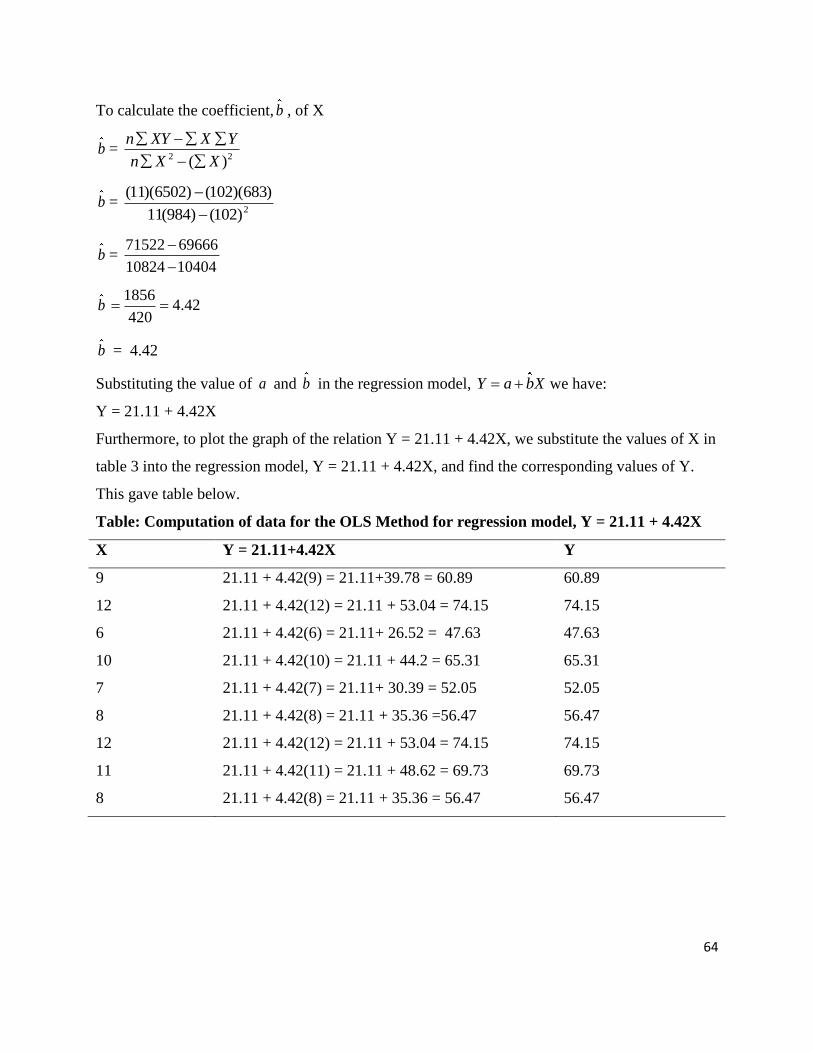
64

To calculate the coefficient, b , of X

b = 2 2( )

n XY X Y

n X X

b = 2

(11)(6502) (102)(683)

11(984) (102)

b = 71522 69666

10824 10404

b1856

4.42420

b = 4.42

Substituting the value of a and b in the regression model, Y a bX we have:

Y = 21.11 + 4.42X

Furthermore, to plot the graph of the relation Y = 21.11 + 4.42X, we substitute the values of X in

table 3 into the regression model, Y = 21.11 + 4.42X, and find the corresponding values of Y.

This gave table below.

Table: Computation of data for the OLS Method for regression model, Y = 21.11 + 4.42X

X Y = 21.11+4.42X Y

9 21.11 + 4.42(9) = 21.11+39.78 = 60.89 60.89

12 21.11 + 4.42(12) = 21.11 + 53.04 = 74.15 74.15

6 21.11 + 4.42(6) = 21.11+ 26.52 = 47.63 47.63

10 21.11 + 4.42(10) = 21.11 + 44.2 = 65.31 65.31

7 21.11 + 4.42(7) = 21.11+ 30.39 = 52.05 52.05

8 21.11 + 4.42(8) = 21.11 + 35.36 =56.47 56.47

12 21.11 + 4.42(12) = 21.11 + 53.04 = 74.15 74.15

11 21.11 + 4.42(11) = 21.11 + 48.62 = 69.73 69.73

8 21.11 + 4.42(8) = 21.11 + 35.36 = 56.47 56.47

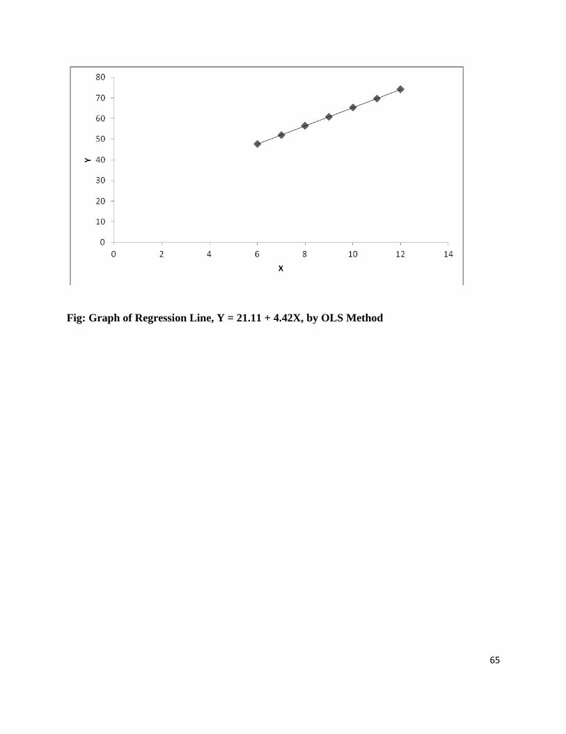
65

Fig: Graph of Regression Line, Y = 21.11 + 4.42X, by OLS Method

66

Method 2: Deviation Method

Table : Data for OLS using Deviation Method

I Y X

y =iY Y

y = Yi - 62.09

x=iX X

x = Xi – 9.27 Xy x2

1. 69 9 69-62.09 = 6.91 9 - 9.27 = -0.27 -1.88 0.073

2. 76 12 76-62.09 =13.91 12-9.27= 2.73 37.97 7.453

3. 52 6 52-62.09 = -10.09 6 - 9.27= -3.27 32.99 10.693

4. 56 10 56-62.09 = -6.09 10-9.27 = 0.73 -4.45 0.533

5. 57 9 57-62.09 = -5.09 9-9.27 = -0.27 1.37 0.073

6. 77 10 77-62.09 =14.91 10-9.27 = 0.73 10.88 0.533

7. 38 7 38-62.09 = -24.09 7-9.27 = -2.27 54.68 5.153

8. 55 8 55-62.09 = -7.09 8-9.27 = -1.27 9.00 1.613

9. 67 12 67-62.09 = 4.91 12-9.27 = 2.73 13.40 7.453

10. 72 11 72-62.09 = 9.91 11-9.27 = 1.73 17.14 2.993

11. 64 8 64-62.09 = 1.91 8-9.27 = -1.27 -2.43 1.613

ƩY= 62.09 ƩX= 9.27

Ʃxy =168.67 Ʃx2= 38.183

The mean of Y is 683

62.0911

Y

NY

The mean of X is 102

9.2722

X

NX

These are the formula used to calculate the parameters of the regression model a

and b

2

xyb

x

a bY X

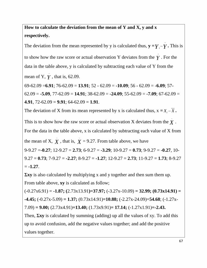
67

How to calculate the deviation from the mean of Y and X, y and x

respectively.

The deviation from the mean represented by y is calculated thus, y =iY Y

. This is

to show how the raw score or actual observation Y deviates from the Y

. For the

data in the table above, y is calculated by subtracting each value of Y from the

mean of Y, Y

, that is, 62.09.

69-62.09 =6.91; 76-62.09 = 13.91; 52 - 62.09 = -10.09; 56 - 62.09 = -6.09; 57-

62.09 = -5.09, 77-62.09 = 14.91; 38-62.09 = -24.09; 55-62.09 = -7.09; 67-62.09 =

4.91, 72-62.09 = 9.91; 64-62.09 = 1.91.

The deviation of X from its mean represented by x is calculated thus, x =iX X .

This is to show how the raw score or actual observation X deviates from the X

.

For the data in the table above, x is calculated by subtracting each value of X from

the mean of X, X

, that is, X

= 9.27. From table above, we have

9-9.27 =-0.27; 12-9.27 = 2.73; 6-9.27 = -3.29; 10-9.27 = 0.73; 9-9.27 = -0.27, 10-

9.27 = 0.73; 7-9.27 = -2.27; 8-9.27 = -1.27; 12-9.27 = 2.73; 11-9.27 = 1.73; 8-9.27

= -1.27.

Ʃxy is also calculated by multiplying x and y together and then sum them up.

From table above, xy is calculated as follow;

(-0.27x6.91) = -1.87; (2.73x13.91)=37.97; (-3.27x-10.09) = 32.99; (0.73x14.91) =

-4.45; (-0.27x-5.09) = 1.37; (0.73x14.91)=10.88; (-2.27x-24.09)=54.68; (-1.27x-

7.09) = 9.00; (2.73x4.91)=13.40; (1.73x9.91)= 17.14; (-1.27x1.91)=-2.43.

Then, Ʃxy is calculated by summing (adding) up all the values of xy. To add this

up to avoid confusion, add the negative values together; and add the positive

values together.

68

Negative values of xy are:

-(1.88+4.45+2.43) = -8.76

Positive values of xy are:

37.97+32.99+1.37+10.88+54.68+9.00+13.40+17.14 = 177.43

Now, add the positive and the negative together, the best way to do this is subtract

the sum of the negative values from the sum of the positive values, that is 177.43-

8.76 = 168.67. So Ʃxy = 168.67.

For Ʃx2, to get the value of sum of x

2, take the square of each value of x, and then

sum them together.

x2 is (-0.27) = 0.073; (2.73)

2 = 7.453; (-3.27)

2 = 10.693; (0.73)

2= 0.533; (-0.27)

2 =

0.073; (0.73)2 = 0.533; (-2.27)

2 = 5.153; (-1.27)

2 = 1.613; (2.73)

2 = 7.453; (1.73)

2

= 2.993; (-1.27)2 = 1.613.

Then sum these values of x2 to get Ʃx

2, that is

0.073+7.453+10.693+0.533+0.073+0.533+5.153+1.613+7.453+2.993+1.613 =

38.183.

Therefore, to calculate the coefficient of, b, of X, we have:

2

xyb

x

= 168.67

4.41738.183

b = 4.42

To calculate the intercept, a , we have:

a bY X

= 62.09 – 4.42(9.27)

a = 62.09- 40.973 =21.117

a = 21.12

69

Substituting the values of a and b in the regression equation, Y a bX , the

regression line becomes;

21.11 4.42Y X

Similarly, to plot the graph of the regression model, 21.11 4.42Y X , we substitute

the values of X in the table into the regression model and find the corresponding

values of Y. Hence, the values of Y are plotted against the values of X on a graph

sheet as in figure .

Example 2: Fit the regression line of the consumption pattern (Y) of a commodity

against the disposable income (X) of the respondents (Consumption pattern, Y is a

function of disposable income X i.e. Y =f(X)) using the following data set below:

Consumption (Y) 12 15 20 22 25 30 35 40 45 50 60 70

Disposable income in

thousands of naira (X)

12 14 18 20 23 28 30 32 35 36 40 45

Solution:

To fit the regression line of Y = f(X). The regression model is assumed to be linear

i.e. Y = a + bX.

Then the least square estimates, a and b should be determined for the regression

line to be fitted.

There are two methods that can be used in the least squares method (OLS) namely:

1. Actual deviation method and

70

2. Deviation method

Method 1: Actual Observation Method

Table 3: Data for OLS Method (Actual Observation Method)

N Consumption (Y) Disposable income (X) XY X2

1. 12 12 12x12 =144 12x12 = 144

2. 15 14 15x14= 210 14x14 = 196

3. 20 18 20x18 = 360 18x18 = 324

4. 22 20 22x22 = 400 20x20 = 400

5. 25 23 25x23 = 575 23x23 = 529

6. 30 28 30x28 = 840 28x28 = 784

7. 35 30 35x30 = 1050 30x30 = 900

8. 40 32 40x32 = 1280 32x32 = 1024

9. 45 35 45x35 = 1575 35x35 = 1225

10. 50 36 50x36 = 1800 36x36 = 1296

11. 60 40 60x40 = 2400 40x40 = 1600

12. 70 45 70x45 = 3150 45x45 = 2025

N=12 ƩY= 424

ƩX = 333

ƩXY = 13824 ƩX2 = 10447

YY

N

=

424

12 = 35.3

XX

N

=

333

12 = 27.75

ƩY = 424; ƩX = 333; ƩXY =13824 ƩX2 = 10447,

To calculate the intercept, a

2

2 2( )

X Y X XYa

n X X

=

2

(10447)(424) (333)(13824)

12(10447) (333)

a = 67072 663204

125364 110889

a = 173864

14475 = -12.011

a = -12.011

To calculate the coefficient b of X

71

b = 2 2 2

(12)(13724) (333)(424)

( ) 12(10447) (333)

n XY X Y

n X X

b165888 141192

125364 110889

b = 24696

1.70614475

b = 1.706

Substituting the value of a and b in the regression model, Y a bX we have:

Y = -12.011 + 1.706X.

Method 2: Deviation Method

Table 4: Data for OLS Method (Deviation Method)

N Consumption

(Y)

Disposable

income (X) ix X X

(x = Xi – 27.75) i

y Y Y

(y = Yi – 35.33)

x2

Xy

1. 12 12 -15.75 -23.33 248.063 367.45

2. 15 14 -13.75 -20.33 189.063 279.54

3. 20 18 -9.75 -15.33 95.063 149.47

4. 22 20 -7.75 -13.33 60.063 103.31

5. 25 23 -4.75 -10.33 22.563 49.07

6. 30 28 0.25 -5.33 0.063 -1.33

7. 35 30 2.25 -0.33 5.063 -0.74

8. 40 32 4.25 4.67 18.063 19.85

9. 45 35 7.25 9.67 52.563 70.11

10. 50 36 8.25 14.67 68.063 121.03

11. 60 40 12.25 24.67 150.063 302.21

12. 70 45 17.25 34.67 297.563 598.06

N =

12 ∑Y= 424

∑X = 333

∑x2 =

1206.25

∑xy =

2058

Y a bX

YY

N

=

424

12 = 35.33

XX

N

=

333

12 = 27.75

72

From table 3, we have:

Ʃxy = 2058, Ʃx2 = 1206.25

(i). To determine the least square estimates, a and b

a bY X

To calculate the coefficient b , of X, we have:

2

20581.706

12065

xyb

x

b = 1.706

Again to calculate the intercept a , we have:

a bY X

a = 35.33 – (1.706)(27.75)

a = 35.33 – (1.706) (27.75)

a = 35.33 -47.3415 = 12.0115

a = -12.01.

Substituting the values of a and b in equation (i), the regression line become

To estimate the equation of the regression lineŶ = a + bX

Ŷ = -12.01 + 1.706X

This implies that a unit increase in disposable income (X) causes 1.706 increase in

the consumption of the commodity in question.

3.2 INTERPRETATION OF PARAMETER ESTIMATES

In a simple regression analysis, we estimate two things: the regression constant (0

) and the regression coefficient (1 ).

73

0 1Y X µt

Where:

0 = Regression constant, 1 = Regression Coefficient

Generally, the regression constant is a real value affecting the dependent variable

determined by some factors outside the relationship between the dependent

variable and the independent or explanatory variable. Regression constant will

have physical meaning to the problem and will be the average value of Y when X

is zero. This is only possible if these two conditions hold:

(i) it must be physically possible for X to equal zero; and

(ii) Data must be collected around X =0

When the two conditions do not hold, the regression constant is then considered as

a real value affecting the dependent variable determined by something outside the

relationship between the dependent and independent variable.

Besides, the regression coefficient (1 ) is used to observe existing difference and

not changes overtime. Rather than talk about a change, we need to talk about two

things that are, at a given point in time, different from each other.

Consider the estimated regression equation below:

Ŷ = 3.72 + 0.94X

Where:

Ŷ = Estimated maize yield (in kg)

X = Amount of fertilizer applied

We can interpret the above regression equation thus:

74

The regression constant 0 =3.72 is the average maize yield when no fertilizer is

applied (i.e. when X = 0). This interpretation is possible since some quantity of

maize will be harvested when no amount of fertilizer is applied to the plot.

On the other hand, the regression coefficient, 1 = 0.94 denotes that if two plots

are treated with different quantities of the same fertilizer such that the quantity of

fertilizer applied to the two different plots differ by 1 unit, then on the average, the

maize yield in the plot with higher quantity of fertilizer will be 0.94kg more than

the maize yield in the plot with smaller quantity of fertilizer.

4.0 CONCLUSION

In this unit you have learnt how to estimate regression parameters of Simple

regression model using both actual observation and deviation methods.

5.0 SUMMARY

In this unit you have learnt that ordinary least square (OLS) method is considered

the best way or technique of obtaining the line of best fit. In using this method

(OLS) to fit regression line, there are two popular approaches that is the actual

observation and deviation approaches of estimating the least square parameters of

simple regression model.


1. a. Use the data in the table below to estimate this model, Y = a + bX

Y 9 12 6 10 9 10 7 8 12

X 69 70 52 56 57 77 38 55 67

b. Interpret the estimated regression model.

75

2. Consider the following regression output:

( ) (0.0976) (0.1961)

ˆ 0.2033 0.6560 tseY X

R2 = 0.397

Where Y = labour force participation rate of women in 2017 and X = the age

of the women sampled.

a. How do you interpret this regression?

b. Test the hypothesis H0: β1 = 1 against H1: β1 > 1. Which test do you use?

And why? What are the underlying assumptions of the test(s) you use?







USA.





76

UNIT 4: PARAMETER TESTING (HYPOTHESIS FORMULATION AND

TESTING)

CONTENTS

1.0 Introduction

2.0 Objectives

3.0 Main content

3.1 Meaning of hypothesis

3.2. Hypothesis Formulation

3.3 Hypotheses Testing

3.3.1 Steps involved in testing of Hypothesis

3.3.2 Standard Error Test

3.3.3 The t-test

3.3.4 The F-test

4.0 Conclusion

5.0 Summary



1.0 INTRODUCTION

In this unit, you learn the meaning of hypothesis; differentiate between null and

alternative hypotheses, how to formulate and test hypotheses with appropriate

statistical tools.

2.0 OBJECTIVES


77

define hypothesis

differentiate between null and alternative hypotheses

formulate hypotheses

apply appropriate statistical tool for testing hypotheses at different level of

significance.

3.0 MAIN CONTENT

3.1. MEANING OF HYPOTHESIS

A hypothesis is a suggested answer or tentative solution to a problem. It is an informed

guess or conjecture about any chosen parameter (e.g. mean) of the population. It is a

tentative supposition or provisional guess which seems to explain the situation under

observation. It is a tentative generalization of the validity of which remains to be tested.

In its most elementary stage the hypothesis may be a guess, imaginative idea which

becomes the basis for further investigation.

Quite often a research hypothesis is a predictive statement, capable of being tested by

scientific methods, that relates an independent variable to some dependent variable.

Within social science, a hypothesis can take two forms, null and alternative hypotheses.

i. Null hypothesis: It can predict that there is no relationship between two variables,

in which case it is a null hypothesis. It is denoted by H0.

A researcher has a null hypothesis when she or he believes, based on theory and

existing scientific evidence, that there will not be a relationship between two

variables. For example, when examining what factors influence a maize farmer‟s

yield within the Federal Capital Territory, Nigeria, a researcher might expect that

farmer‟s level of education (in years of schooling) would NOT have an impact on

maize yield. This would mean the researcher has stated the null hypotheses.

ii. Alternative hypothesis: It can predict the existence of a relationship between

variables, which is known as an alternative hypothesis. It is denoted by HA or H1.

But when examining what factors influence a maize farmer‟s yield within the

78

Federal Capital Territory, Nigeria, a researcher might expect that farmer‟s level of

education (in years of schooling) would have an impact on maize yield. In this

case, educational attainment is an independent variable, and farmer‟s maize yield

is the dependent variable --it is hypothesized to be dependent on the farmer‟s level

of education.

Researchers seek to determine whether or not their hypothesis, or hypotheses if they have

more than one, will prove true. Sometimes they do, and sometimes they do not. Either

way, the research is considered successful if one can conclude whether or not a

hypothesis is true.

3.2 Formulating a hypothesis:

It can take place at the very beginning of a research project, or after a bit of

research have already been done.

Sometimes a researcher knows right from the start which variables he is interested

in studying, and he may already have a hunch about their relationships.

Other times, a researcher may have an interest in a particular topic, trend, or

phenomenon, but he may not know enough about it to identify variables or

formulate a hypothesis.

Whenever a hypothesis is formulated, the most important thing is to be precise about

what one's variables are, what is the nature of the relationship between them might be,

and how one can go about conducting a study on them.

3.3 HYPOTHESES TESTING

Before explaining the common statistical tools to tests hypothesis, there are steps

involved in testing hypotheses.

79

3.3.1 Steps involved in testing hypothesis

1. Clearly formulate and state the hypotheses (i.e. both null and alternative

hypotheses).

2. Choose the method of statistical test to use

3. Choose the level of significance to use in testing the formulated hypothesis

4. Calculate the value of the chosen statistical test to test the hypothesis

5. State decision rule to decide the acceptance or rejection of the null hypothesis.

6. Compare the calculated value with the theoretical or table value.

7. Make conclusion on the acceptance and the rejection of the null hypothesis.

In this section, the three common tests shall be considered. These are:

i. the standard error test

ii. the t-test and

iii. the F-test.

During hypothesis testing, we are faced with the task of finding out whether the

parameter estimates are statistically significant or not. Hence it entails determining

whether the independent variable(s) significantly affect the dependent variable or not.

3.3.2 Standard Error Test

In this test, no reference is made to degree of freedom. A comparison is made between

the parameter estimate and its standard error. Based on the result of the comparison

judgment is passed on the significance of the estimate.

80

Decision Rule

a. If the standard error of β1 greater than the half of the coefficient of β1 (that is,

11

2S

), we reject the null hypothesis (H0) and conclude that

1 is not

statistically significant.

b. If 11

2S

, we reject H0, i.e., accept HA; and conclude that

1 is statistically

significant.

3.3.3 The t-test

Here, reference is made to the degree of freedom at the chosen level of significance. The

calculated t-value is compared with the theoretical (t-tab) t-value at a particular or

defined level of significance with (n-k) degree of freedom. The calculated t-value is given

by:

t* cal=

1

1S

Decision Rule

(a)If t*cal>t tab, we reject the null hypothesis (H0) and conclude that 1 is

statistically significant, that is 1 is different from zero.

(b) If t*cal <t tab, we accept the null hypothesis (H0) and conclude that 1 is not

statistically significant, that is; 1 is not different from zero.

However, t-test is usually used when the number of observations, n≤30.

3.3.4 The F-test

This is usually used to test the OVERALL significance of a regression model. It is

employed to determine whether all the 'i s are zero or not. It is equally based on the

81

value of the degree of freedom and the percentage level of significance chosen. The

calculated F*-value (F-cal) is compared with the theoretical F-value (F-tab).

The F-calculated (F-cal) is determined by:

F*cal =

2

2

( 1)

1

R k

R N k

F*cal =

2

2

( )

1 1

R N k

R k

Decision Rule

(a) If F*cal>F-tab, reject the null hypothesis (H0) and conclude that not all i

are zero. i.e., the OVERALL regression is statistically significant.

(b) If F*cal<F tab, accept the null hypothesis (H0) and conclude that the

OVERALL regression is not statistically significant.

NB: Before attempting to test the parameter estimates, the hypothesis must be clearly

formulated and stated. E.g.

H0: βi = 0

HA: βi ≠ 0

Worked Example: Given that (0.905) (0.13)0.096 0.34Y

is an estimated import demand function, test the hypothesis on the independent variable

(NB: R2 = 0.76).

Solution:

Method 1: The Standard Error test

Step 1: State clearly the hypotheses

Null hypothesis (H0): βi = 0.

Alternative hypothesis (HA): βi ≠ 0

82

Step 2: Choose the method statistical test to use. Here it is Standard Error test.

Step 3: There is no need for selection of level of significance for this test to hold.

Step 4: Calculate the value of the chosen statistical test to test the hypothesis.

Note that the values in the parentheses are standard errors. That is; For the

parameter β1, the standard error S(1 ) = 0.13; and the coefficient of the

independent variable, β1 is 1 = 0.34.

1

2

=

0.340.17

2

Step 5: State decision rule to decide the acceptance or rejection of the null hypothesis.

Decision Rule:

i. If the standard error of β1 greater than the half of the coefficient of β1 (that

is, 11

2S

), we accept the null hypothesis (H0) and conclude that

1 is

not statistically significant.

That is, 11

2S

), we accept H0.

ii. If 11

2S

, we reject H0, i.e., accept HA; and conclude that

1 is

statistically significant.

Step 6: Compare the calculated value with the theoretical or table value. In

Standard Error Test, we only compare the values of 11

2S and

to take decisions

and not the theoretical and the calculated values.

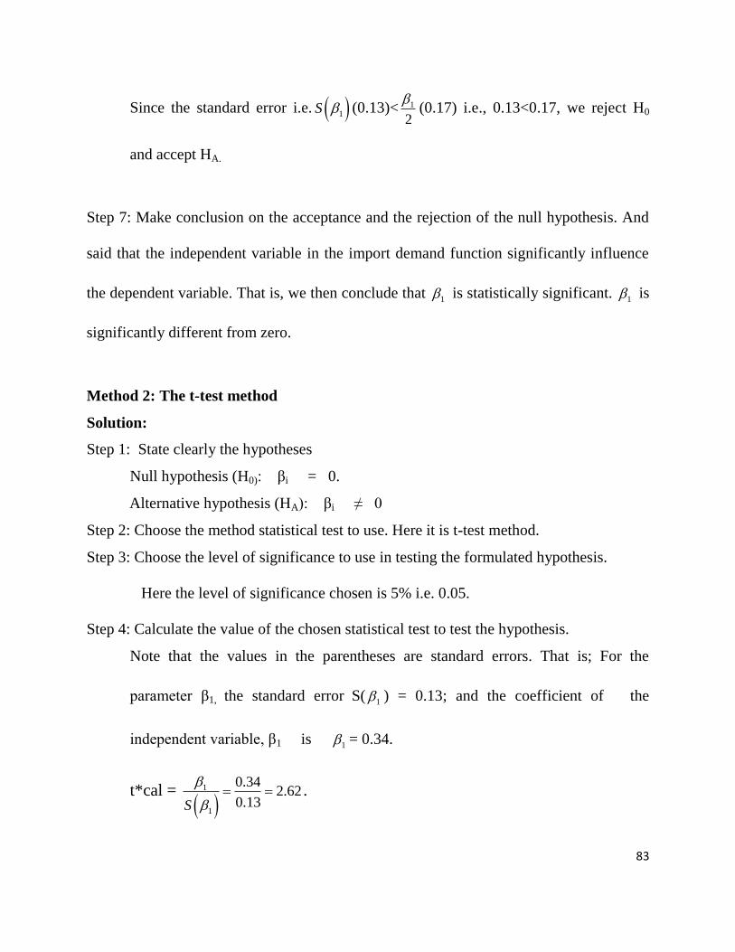
83

Since the standard error i.e. 1S (0.13)< 1

2

(0.17) i.e., 0.13<0.17, we reject H0

and accept HA.

Step 7: Make conclusion on the acceptance and the rejection of the null hypothesis. And

said that the independent variable in the import demand function significantly influence

the dependent variable. That is, we then conclude that 1 is statistically significant.

1 is

significantly different from zero.

Method 2: The t-test method

Solution:

Step 1: State clearly the hypotheses

Null hypothesis (H0): βi = 0.

Alternative hypothesis (HA): βi ≠ 0

Step 2: Choose the method statistical test to use. Here it is t-test method.

Step 3: Choose the level of significance to use in testing the formulated hypothesis.

Here the level of significance chosen is 5% i.e. 0.05.

Step 4: Calculate the value of the chosen statistical test to test the hypothesis.

Note that the values in the parentheses are standard errors. That is; For the

parameter β1, the standard error S(1 ) = 0.13; and the coefficient of the

independent variable, β1 is 1 = 0.34.

t*cal =

1

1

0.342.62

0.13S

.

84

At 5% level of significance and (n-k = 10-2) = 8 degree of freedom, t-tab = 2.306

i.e. t0.025=2.306.

Step 5: State decision rule to decide the acceptance or rejection of the null hypothesis.

Decision Rule:

If t*cal> t tab, reject H0; accept HA; and

If t*cal<t tab accept H0.

Step 6: Compare the calculated value with the theoretical or table value. Since t* cal =

2.62 and t-tab =2.306, then, 2.62>2.306, we then say t*cal>t tab, we then reject H0 and

accept HA.

Step 7: Make conclusion on the acceptance and the rejection of the null hypothesis.

We then conclude that the independent variable in the import demand function

significantly influence the dependent variable. That is, we then conclude that 1 is

statistically significant. It shows that1 is significantly different from zero. (Similarly, we

conclude that β is statistically significant; it is different from zero).

Method 3: F-test Method

F*cal =

2

2

( )

1 1

R N k

R k

In using F-test, two degrees of freedom need to be determined. These are

V1 = k−1 and V2 =N−K

Where:

N= Number of observations

K= Number of variables

F*cal =

2

2

( )

1 1

R N k

R k

=

(0.76)(10 2)

(1 0.76)(2 1)

85

F*cal = (0.76)(8) 6.08

25.33(0.24)(1) 0.24

F*cal = 25.33

At 5% level of significance, V1 = k−1 =2−1 =1 and V2 =N−k =10 −2= 8 degrees of

freedom,

Check the F-table under the degree of freedom, V1 = 1, V2 = 8, the theoretical value is F-

tab =5.32

Decision Rule

If F*cal>F tab, reject H0, then accept HA

If F*cal< F tab, accept H0.

Since 25.33>5.32

i.e.,

F*cal > F tab, we reject H0 and accept HA. We then conclude that the overall

regression is statistically significant.

4.0 CONCLUSION

In this unit, you have learnt the meaning of hypothesis; differentiate between null and

alternative hypotheses, how to formulate and test hypotheses with appropriate statistical

tools (t-test, standard error test and F-test).

5.0 SUMMARY

In this unit you have learnt that a hypothesis is a suggested answer or tentative solution to

a problem. It is an informed guess or conjecture about any chosen parameter (e.g. mean)

of the population.

Steps involved in testing hypothesis are:

1. Clearly formulate and state the hypotheses (i.e. both null and alternative

hypotheses).

86

2. Choose the method of statistical test to use

3. Choose the level of significance to use in testing the formulated hypothesis

4. Calculate the value of the chosen statistical test to test the hypothesis

5. State decision rule to decide the acceptance or rejection of the null hypothesis.

6. Compare the calculated value with the theoretical or table value.

7. Make conclusion on the acceptance and the rejection of the null hypothesis

The three common tests considered are:

i. the standard error test

ii. the t-test and

iii. the F-test


1. Explain what an hypothesis is

2. Differentiate between the following:

i. t-test and Z-test

ii. t-test and F-test

iii. null and alternative hypotheses

3. Enumerate and discuss steps involved in using t-statistic to test an hypothesis

4. Given that (7.5) (0.03)13.53 0.097Y

is an estimated consumption function, test the hypothesis on the independent

variable at 5% level of significance (NB: R2 = 0.99).





Edition,

Tata McGraw Hill Educational Private Limited, New Delhi, India.

87

Koop, G. (2000). Analysis of Economic Data. John Willey & Sons Ltd, New York, USA.

Osuala, A. E. (2010). Econometrics: Theory and Problems. ToniPrints Services, Abia

State, Nigeria.


Edition,

South-Western Centage Learning, Mason, USA.

88

MODULE 4: CORRELATION ANALYSIS

Unit 1 The meaning of Correlation

Unit 2 Types/forms of Correlation

Unit 3 Computational Procedures

Unit 4 Test of Significance of Correlation Coefficient

Unit 5 Limitations of Linear Correlation and Correlation versus Regression

UNIT 1 THE MEANING OF CORRELATION

CONTENTS

1.0 Introduction

2.0 Objectives

3.0 Main content

3.1 Definition and scope of correlation

4.0 Conclusion

5.0 Summary



1.0 INTRODUCTION

Another area of interest in this study of Econometrics is how variables and observations

are related. This unit is important because it helps to understand the meaning of

correlation. Understanding this will help you to perform basic statistical procedure for

establishing the relationship between variables.

89

2.0 OBJECTIVES


describe what correlation is

understand the scope of correlated variables.

3.0 MAIN CONTENT

3.1 DEFINITION AND SCOPE OF CORRELATION

Correlation is a measure of the degree of relationship existing between two variables. It

could be defined as the degree to which variables are related hence, it is an index for

measuring the degree to which variables are associated.

Just like in regression analysis, a relationship can exist between two variables (that is

between one dependent variable and one independent variable). When the relationship is

between two variables it is termed a simple correlation. For instance, the consumption

theory stipulates that level of consumption is a function of income level. Mathematically,

this theory can be presented thus;

C = f(Y)

Where C = Consumption level

Y = Income level.

Therefore, in the above equation, there are only two variables namely consumption, C

and Income, Y. Hence the degree of relationship existing between C and Y is termed

simple correlation.

90

On the other hand, if the relationship is between more than two variables, it is called a

multiple correlation. Consider the production function.

Total output, TP = f (L, L*, K, M)

Where

L = Land

L* = Labour

K = Capital

M = Management

From the equation above, there are five variables namely; total output (TP), Land(L),

Labour(L*), Capital (K) and Management (M). The degree of relationship between these

variables is termed a multiple correlation.

4.0 CONCLUSION

In this unit you have learnt about basic fundamentals of correlation; and to distinguish

simple and multiple correlation

5.0 SUMMARY

Therefore at this end I believe you must have understood the meaning and scope of

correlation.


i. What do you understand by correlation?

ii. Differentiate between simple correlation and multiple correlations.

91





Edition,



State, Nigeria.

92

UNIT 2: TYPES/ FORMS OF CORRELATION

1.0 Introduction

2.0 Objectives

3.0 Main content

3.1 Linear correlation

3.2 Non-linear correlation

3.3 Zero correlation

4.0 Conclusion

5.0 Summary



1.0 INTRODUCION Having learnt about the meaning of correlation in the previous unit, it is necessary to

learn about the types of correlation. This will enable you to appreciate the meaning of

linear, non-linear and zero correlation.

2.0 OBJECTIVE


describe the types and forms of correlation.

3.0 MAIN CONTENT

3.1 Linear correlation

93

Correlation is considered linear when all points on a scattered diagram seem to cluster

near a straight line. However, a relationship could either be positive or negative. Two

variables are said to be linearly and positively correlated if they tend to move in the same

direction. In other words, the two typical example exists in the supply function, Qs= f(P).

In this function, an increase in the price of the commodity leads to an increase in the

quantity of the commodity supplied, ceteris paribus.

Diagrammatically, the positive linear correlation is represented thus;

Y

X

Fig. 4.1: Positive linear correlation between X and Y

In figure 4.1 above, it could be seen that not all the points on the scatter diagram fall on

the straight line. This shows that the correlation between X and Y is not perfect. If all the

points fell on the straight line, the correlation is said to be perfect positive.

Besides, two variables are said to be negatively and linearly correlated if the two

variables tend to move in the opposite direction. Thus, if one of the variables is

94

increasing the other variable will be decreasing showing an inverse relationship between

the two variables. This type of relationship is shown by the demand function. Qd = f(P).

The demand theory states that the higher the price of a commodity, the lower will be the

quantity demanded. Therefore, there is an inverse relationship existing between price, P

and quantity demanded, Qd.

Diagrammatically, a negative lines correlation can be shown thus;

Y

X

Fig. 4.2 Negative Linear Correlation between X and Y

Equally, all points do not fall on the straight liner. Hence, the relationship is not perfect.

If all the points fall on the straight line, the correlation is said to be perfect negative.

3.2 Non-linear Correlation

Correlation between two variables is said to be non- linear when all points seem to lie

near a curve. As in linear correlation, non-linear correlation could be positive or negative.

The correlation between two variables, X and Y is said to be positive non-linear if they

move in the same direction described by a curve.

95

The diagram of this type of correlation is shown below:

Y

X

Fig.4.3: Positive non-linear Correlation between X and Y

Also, two variables are negatively non-linearly correlated when they move in opposite

directions (that is) an inverse relationship along a curve.

Y

X

96

Fig. 4.4: Negative non-linear Correlation

3.3 Zero Correlation

This type of correlation occurs when two variables are uncorrelated with each

other. In other words, there is no relationship between the two variables. On the

scattered diagram, the points are dispersed all over the surface of the SY plane with

no suitable line to join them hence, the term zero correlation.

Y

X

Fig. 4.5: Zero Correlation

4.0 CONCLUSION

In this unit you have learnt about the types/forms of correlation. You have learnt about

what differentiate linear, non-linear and zero correlation.

5.0 SUMMARY

In this unit you have learnt that correlation has three basic types (linear, non-linear and

zero/no correlation).

97


1. With the aid of diagram, explain what you understand by the following:

i. linear positive correlation

ii. linear negative correlation

iii. non-linear correlation

iv. zero correlation





Edition,




State, Nigeria.

98

UNIT 3: PROCEDURES FOR COMPUTING CORRELATION

COEFFICIENT, r


2.0 Objectives

3.0 Main content

3.1 Methods of Computing Correlation Coefficient

3.2 Pearson‟s Product Moment Correlation Coefficient

3.2.1 Deviation Method

3.2.2 Direct Observation

3.3 Rank Spearman‟s Correlation Coefficient

4.0 Conclusion

5.0 Summary



1.0 INTRODUCTION

This unit is aimed at addressing the two approaches of computing correlation coefficient,

and the Pearson‟s Product Correlation Coefficient method using both direct observation

and the deviation methods. You will also understand that when the observations are not

quantitative, that is, qualitative, that the Rank Spearman Correlation Coefficient is to be

applied.

2.0 OBJECTIVES


know the approaches of computing correlation coefficient

99

compute Pearson‟s Product Correlation Coefficient method using both direct

observation and the deviation methods.

understand when to use the Rank Spearman Correlation Coefficient.

3.0 MAIN CONTENT

3.1 Methods of Computing Correlation Coefficient

The magnitude of the correlation existing between variables is termed the correlation

coefficient. This coefficient measures the degree of co-variability of two variables, X and

Y. The correlation coefficient has a range from +1 to -1 i.e. -1 ≤ r ≤ 1.

To calculate this correlation coefficient, two approaches could be taken.

Approach 1: Finding the square root of the coefficient of determination.

Approach 2: Calculating directly from the definitional formula of correlation coefficient.

It is however, important to note that these computational procedures are used for

variables which are quantitative in nature. In this course material, the second approach is

used to compute the correlation coefficient, r using the deviation method and the direct

observation method.

3.2 Pearson’s Product Moment Correlation Coefficient

In calculating correlation coefficient using Pearson‟s Product Moment Correlation

Coefficient, there are two methods to use, the direct observation and the deviation

method. The procedures for computing these two methods are addressed through the

worked example below.

Worked Example: The table below shows the output, Y obtained at different levels of

variable input, X.

100

Table 4.1: Data for Output, Y of maize and Input, X (Labour)

X(Mondays) 1 2 3 4 5 6 7 8 9 10

Y(tons) 13 17 21 38 37 27 33 21 16 17

Calculate the correlation coefficient for the relationship existing between X and Y

Solution:

3.2.1 The Deviation Method

Procedures for Computing the correlation coefficient, r using deviation method are as

follow:

State the formula

2 2( )( )

xyr

x y

Know the number of the observation, i.e. N

Calculate the mean of the two variables X and Y, that is X and Y respectively.

X

XN

and

YY

N

Calculate the deviations x and y of the two variables X and Y from the mean for

each under X and Y. That x = X- X and y = Y -Y

Square the deviations x and y, that is x2

and y2, then obtain the sum of the squared

deviation, that is Ʃx2 and Ʃy

2.

Multiply each deviation under x with each deviation under y and obtain the

product of xy. Then obtain the sum of the product of xy i.e. Ʃxy.

101

Substitute the values of Ʃxy, Ʃx2, and Ʃy

2 into the formula.

Table 4.2: Basic Calculations to Obtain the Correlation Coefficient Using the

Deviation Method

X Y x= X-X

x = X- 5.5

y =Y-

y= Y- 23

Xy x² y²

1 13 1-5.5 = -4.5 13-10 = -10 -4.5x -10 =45 -4.5x-4.5= 20.25 -10 x-10 = 100

2 17 2-5.5 = -3.5 17-23 = -6 -3.5x-6=21 -3.5x-3.5= 12.25 -6 x-6 = 36

3 21 5.5 – 3 = -2.5 21-23 = -2 -2.5 x-2= 5 -2.5x-2.5 = 6.25 -2 x-2 = 4

4 38 4-5.5 = -1.5 38-23 =15 -1.5x15 = -22.5 -1.5x-1.5 = 2.25 15 x 15 = 225

5 37 5-5.5 = -0.5 37-23 = 14 -0.5x14 = -7 -0.5x-0.5= 0.25 -14 x 14 = 196

6 27 6-5.5 = 0.5 27-23 = 4 0.5 x 4 =2 0.5x0.5= 0.25 4 x 4 = 16

7 33 7-5.5 = 1.5 33-23 = 10 1.5 x 10 =15 1.5x1.5 = 2.25 10 x 10 = 100

8 21 8-5.5 = 2.5 2-23 = -2 2.5 x -2 = -5 2.5x2.5 = 6.25 -2 x -2 = 4

9 16 9-5.5 = 3.5 16-23 = -7 3.5 x -7 = -24.5 3.5x3.5 = 12.25 -7x -7 = 49

10 7 10-5.5 = 4.5 7-23 = -16 7 x 4.5 = -72 4.5x4.5 = 20.25 -16 x -16 =

256

ƩX=55 ƩY= 230 Ʃxy = -43 Ʃx2 = 82.5 Ʃy

2 = 986

555.5

10

XX

N

23023

10

YY

N

2 2( )( )

43 43

(82.5)(986) 81345

430.15

285.2

0.15

xyr

x y

r

r

r

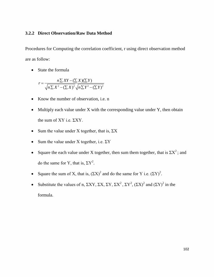
102

3.2.2 Direct Observation/Raw Data Method

Procedures for Computing the correlation coefficient, r using direct observation method

are as follow:

State the formula

2 2 2 2

( )( )

( ) ( )

n XY X Yr

n X X n Y Y

Know the number of observation, i.e. n

Multiply each value under X with the corresponding value under Y, then obtain

the sum of XY i.e. ƩXY.

Sum the value under X together, that is, ƩX

Sum the value under X together, i.e. ƩY

Square the each value under X together, then sum them together, that is ƩX2 ; and

do the same for Y, that is, ƩY2.

Square the sum of X, that is, (ƩX)2 and do the same for Y i.e. (ƩY)

2.

Substitute the values of n, ƩXY, ƩX, ƩY, ƩX2

, ƩY2, (ƩX)

2 and (ƩY)

2 in the

formula.

103

Table 4.3: Basic Calculations to Obtain the Correlation Coefficient Using the Direct

Observation/Raw Data Method

X Y X² Y² XY

1 13 1x1= 1 13x13 =169 13x1= 13

2 17 2x2= 4 17x17 =289 2x17= 34

3 21 3x3= 9 21x21 =441 3x21= 63

4 38 4x4= 16 38x38 =1444 4x38= 152

5 37 5x5= 25 37x37 =1369 5x37= 185

6 27 6x6= 36 27x27 =729 6x27= 162

7 33 7x7=49 33x33 =1089 7x33= 231

8 21 8x8=64 21x21 =441 8x21= 168

9 16 9x9=81 16x16 =256 9x16= 144

10 7 10x10=100 7x7 =49 10x7= 70

ƩX= 55 ƩY= 230 ƩX2 = 385 ƩY

2 = 6276 ƩXY= 1222

2 2 2 2

2 2

( )( )

( ) ( )

10(1222) (55)(230)

10(385) (55) 10(6276) (230)

12220 12650

(3850) (3025) (62760) (52900)

430 430

(28.72)(99.30)825 9860

4300.15

2851.90

0.15

n XY X Yr

n X X n Y Y

r

r

r

r

r

555.5

10

23023

10

XX

N

YY

N

104

From the values of r in both approaches, it could be discovered that we obtained the same

quantity (magnitude) for the correlation coefficient.

From the two methods, the value of r is the same. It shows that the correlation between X

and Y is weak negative correlation.

3.3 Rank Correlation Coefficient (Spearman’ Correlation Coefficient)

In the correlation analysis discussed above, it is assumed that the variables involved are

quantitative and thus, their data can be measured with some accuracy. However, there are

variables, which may be qualitative in nature and hence, have no numerical

measurements or values.

In order to determine the nature of correlation between these qualitative variables, it is

impossible to use the methods discussed earlier. Rather, another statistical tool called the

rank correlation coefficient, r is employed to analyse the magnitude and the nature of the

correlation.

This statistical tool or technique requires that the observations be ranked in a specific

sequence. After assigning ranks to the observations, we can then measure the relationship

between the observations‟ ranks instead of their actual numerical values.

If two variables are ranked, their rank (Spearman‟s) correlation coefficient can be

calculated from the formula;

2

2

61

( 1)

Dr

n n

Where:

D = difference between ranks of corresponding pairs of X and Y.

n = Number of observations

The values of r has a range of -1≤ r ≥1.

In applying this method of correlation analysis, it is necessary to note that:

(i). it does not matter whether the observations are ranked in ascending or descending

order. However, the same rule of ranking must be used for both variables; and

105

(ii). if two or more observations have the same value, we assign to them rank.

Worked Example:

The following table shows the ranking preference of two consumers for five (5) different

locally produced brands of rice namely; LAKE rice (L), EBONYI (E), OFADA (O),

UMZA rice (U) and LABANA (B).

Brands locally produced of Rice L E O U B

Ranking of Consumer A 1 3 2 5 4

Ranking of Consumer B 2 1 3 4 5

Solution:

The differences between the ranking of the two consumers is given by:

Difference, D = Ranking of Consumer A – Ranking of Consumer B,

The difference, D is shown below:

Table 4.4: Data for Estimating Spearman Rank Correlation

Brands locally produced of Rice L E O U B

Ranking of Consumer A 1 3 2 5 4

Ranking of Consumer B 2 1 3 4 5

Difference, D -1 2 -1 1 -1

D2

1 4 1 1 1

ƩD2 1+4+1+1+1 = 8

ƩD2 = 8

Applying the formula, we have:

2

2

61

( 1)

Dr

n n

106

481

5(25 1)

481

5(24)

481

120

1 0.4

0.6

r

r

r

r

r

Therefore, the rank correlation coefficient, 0.6r and this shows a fairly similar

preferences of the two consumers (A and B) for the five brands of locally produced rice

under consideration. Note that the existing relationships or correlation is positive and also

strong.

4.0 CONCLUSION

In this unit, you have learnt the two approaches of computing correlation coefficient, and

the Pearson‟s Product Correlation Coefficient method using both direct observation and

the deviation methods. You have also learnt that the Rank Spearman Correlation

Coefficient method is used when the observations are qualitative.

5.0 SUMMARY

In this unit you have learnt that correlation coefficient measures the magnitude of the

correlation existing between variables. This coefficient measures the degree of co-

variability of two variables, X and Y. The correlation coefficient has a range from +1 to -

1 i.e. -1 ≤ r ≤ 1.

To calculate this correlation coefficient, two approaches could be taken.

Approach 1: Finding the square root of the coefficient of determination.

Approach 2: Calculating directly from the definitional formula of correlation coefficient.

The Second approach is the one addressed in this course material.

107

In calculating correlation coefficient using Pearson‟s Product Moment Correlation

Coefficient, two methods are used, the direct observation and the deviation methods.

The procedures computing the correlation coefficient, r using deviation method are as

follow:

i. State the formula

a. 2 2( )( )

xyr

x y

ii. Know the number of the observation, i.e. N

iii. Calculate the mean of the two variables X and Y, that is X and Y respectively.

a. X

XN

and

YY

N

iv. Calculate the deviations x and y of the two variables X and Y from the mean for

each under X and Y. That x = X- X and y = Y -Y

v. Square the deviations x and y, that is x2

and y2, then obtain the sum of the squared

deviation, that is Ʃx2 and Ʃy

2.

vi. Multiply each deviation under x with each deviation under y and obtain the

product of xy. Then obtain the sum of the product of xy i.e. Ʃxy.

vii. Substitute the values of Ʃxy, Ʃx2, and Ʃy

2 into the formula.

The procedures for computing the correlation coefficient, r using the direct/actual

observation method are as follow:

i. State the formula

a. 2 2 2 2

( )( )

( ) ( )

n XY X Yr

n X X n Y Y

108

ii. Know the number of observation, i.e. n

iii. Multiply each value under X with the corresponding value under Y, then obtain

the sum of XY i.e. ƩXY.

iv. Sum the value under X together, that is, ƩX

v. Sum the value under X together, i.e. ƩY

vi. Square the each value under X together, then sum them together, that is ƩX2

; and

do the same for Y, that is, ƩY2.

vii. Square the sum of X, that is, (ƩX)2 and do the same for Y i.e. (ƩY)

2.

viii. Substitute the values of n, ƩXY, ƩX, ƩY, ƩX2, ƩY

2, (ƩX)

2 and (ƩY)

2 in the

formula.

When the variables are qualitative in nature and hence, have no numerical measurements

or values, in order to determine the nature of correlation between these qualitative

variables, it is impossible to use Pearson‟s Product Moment Correlation Coefficient.

Rather, another statistical tool called the rank correlation coefficient, r is employed to

analyse the magnitude and the nature of the correlation.


1. The following table shows how ten farmers were ranked according to their

adoption of rice technology in an area and their paddy yield in the season under

consideration.

Farmers A B C D E F G H I J

Ranking based on adoption 2 5 6 1 4 10 7 9 3 8

Ranking based on yield of paddy rice 1 6 4 2 3 7 8 10 5 9

109

i. Which correlation coefficient method will you use to determine the magnitude and

nature of the relationship between the adoption of rice technology and the yield of

paddy rice?

ii. Determine the correlation coefficient of the adoption of rice technology and the

yield of paddy rice.

iii. Test the significance of the correlation coefficient of the adoption of rice

technology and the yield of paddy rice at 5% level of significance.

2. Based on the data in the table below,

Time period (days) 1 2 3 4 5 6 7 8 9 10

Quantity supplied (tons) Y 10 20 50 40 50 60 80 90 90 120

Price in Naira (X) 2 4 6 8 10 12 14 16 18 20

Determine the following:

i. Compute the correlation coefficient for the following data on quantity

supplied in tons and the price in naira of rice for 10 days by a marketer.

ii. Test the significance of the correlation coefficient at 5 % level of

significance.


Awoke, M. U. (2002). Econometrics: theory and application. Willy & Appleseed



Edition,



Koutsoyiannis, A. (2001). Theory of econometrics: an introductory exposition of

econometric methods (2nd

edition). Plagrave, Hampshire, New York, USA.


State, Nigeria.

110


Edition,


111

UNIT 4: TEST OF SIGNIFICANCE OF CORRELATION COEFFICIENT

CONTENTS

1.0 Introduction

2.0 Objectives

3.0 Main content

3.1 The use of t-statistic for test of significance of correlation coefficient

3.2. The use of Z-statistic for test of significance of correlation coefficient

4.0 Conclusion

5.0 Summary



1.0 INTRODUCTION

In this unit, you learn when to use t-statistic and Z-statistic for test of significance of

correlation coefficient. It is necessary to understand that t-statistic is used to test of

significance of correlation coefficient when the true population is zero. And Z-statistic is

used to test for the significance of rank correlation, r‟.

2.0 OBJECTIVES


understand when to use t-statistic and z-statistic for test of significance of

correlation coefficient.

112

3.0 MAIN CONTENT

3.1. APPLICATION OF t-STATISTIC FOR TEST OF SIGNIFICANCE OF

CORRELATION COEFFICIENT

The correlation coefficients measure the degree of relationship between samples drawn

from a population. It is therefore, necessary that we find out their statistical reliability by

conducting some test of significance. This test of significance also helps us to make a

reliable conclusion about the population.

A correlation coefficient may be tested to determine whether the coefficient significantly

differs from zero. The value r is obtained on a sample. The value rho (ρ) is the

population's correlation coefficient. It is hoped that r closely approximates rho (ρ).

The null and alternative hypotheses are as follows:

Ho: ρ = 0

Ha: ρ ≠ 0

The value of r and the number of pairs of scores are converted through a formula into a

distribution (similar to the z distribution) called the t distribution. The t formula can only

be used to test whether r is equal to zero. It cannot be used to test to see whether r might

be equal to some number other than zero.

It is also important to note that the t distribution may be used to test other types of

inferential statistics. Therefore, if someone says that a t-test is being used, it would be a

legitimate question to ask “why?” The t distribution is most commonly used to test

whether two means are significantly different, however, it may also be used to test the

significance of the correlation coefficient. Interestingly, the t distribution becomes z

113

distribution when the data is infinite but they are also strikingly visually similar when

there are only several hundred numbers in the set of data. The t-test formula in order to

test the null hypothesis for a correlation coefficient is:

*

2

2

1

r nt cal

r

In making our decision regarding the significance or non-significance of the correlation

coefficient, we need the theoretical (table) value, tα/2 at (n-2) degree of freedom (df).

For a two-tailed test at 5% level of significance, tα/2 becomes:

α = (1-95%)

α = (1-95/100)

α = (1-0.95)

α = 0.05

Therefore,

tα/2 = t0.05/2 = t0.025

Worked Example: Test the statistical reliability of the sample correlation coefficient r =

0.15 and n=15.

Solution:

r = 0.15

n=15.

114

*

2

2

2

1

0.15 10 2

1 (0.15)

0.15 8

1 0.0225

0.15(2.828)

0.9775

0.42420.429

0.9887

0.43

r nt cal

r

tcal

tcal

tcal

tcal

tcal

3.2. APPLICATION OF Z-STATISTIC FOR TEST OF SIGNIFICANCE

OF CORRELATION COEFFICIENT

To test for the significance of the rank correlation coefficient, r', we employ the use of a

different statistic called the Z-statistic provided that the sample size is large.

The Z-statistic is given by:

* 1Z r n

Where:

r' = rank correlation coefficient

n = number of observation

Decision Rule: If -1.96≤ Z* ≥ 1.96, we accept H0. Otherwise we reject H0,

Worked Example: Test the level of significance, (when r′ =0.6 and n = 5, from the

example solved above).

Solution:

r′ =0.6

n = 5

115

Therefore,

*

*

*

*

*

1

0.6 5 1

0.6 4

0.6(2) 1.2

1.2

Z r n

Z

Z

Z

Z

Decision Rule:

If -1.96≤ Z* ≥ 1.96, we accept H0. Otherwise we reject H0, that is, r

′ = 0.

But, Z* = 1.2 which means

Z* > -1.96

Z* < 1.96.

Therefore,

-1.96≤ (1.2 = Z*) ≥ 1.96

Conclusion:

We then accept the null hypothesis H0 and reject the alternative hypothesis. This means

that the rank correlation coefficient is not statistically significant.

4.0 CONCLUSION

In this unit you have learnt about the test of significance of correlation coefficients of

both the Pearson‟s Product Moment Correlation coefficient and the Rank Spearman

Correlation Coefficient using t-statistic and Z-statistic respectively. You have also learnt

using Z-statistic when the sample size is large.

5.0 SUMMARY

In this unit you have learnt about the Pearson‟s Product Moment Correlation Coefficient

method especially useful for qualitative variables.

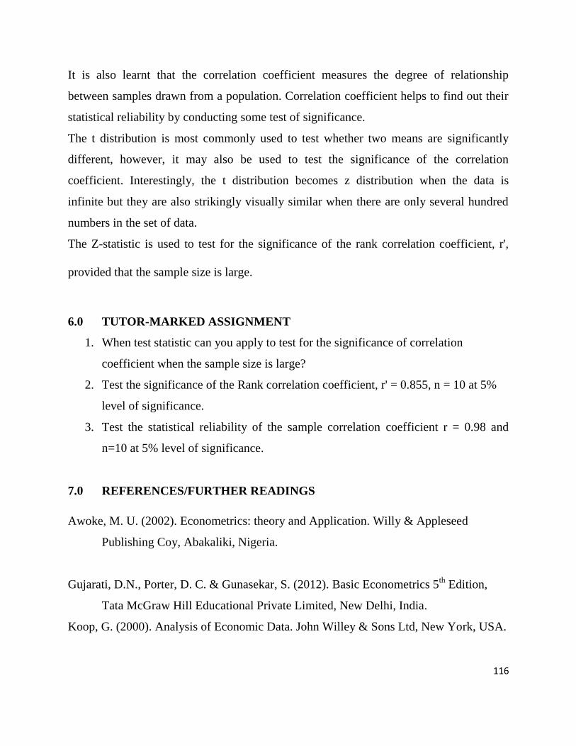
116

It is also learnt that the correlation coefficient measures the degree of relationship

between samples drawn from a population. Correlation coefficient helps to find out their

statistical reliability by conducting some test of significance.

The t distribution is most commonly used to test whether two means are significantly

different, however, it may also be used to test the significance of the correlation

coefficient. Interestingly, the t distribution becomes z distribution when the data is

infinite but they are also strikingly visually similar when there are only several hundred

numbers in the set of data.

The Z-statistic is used to test for the significance of the rank correlation coefficient, r',

provided that the sample size is large.


1. When test statistic can you apply to test for the significance of correlation

coefficient when the sample size is large?

2. Test the significance of the Rank correlation coefficient, r' = 0.855, n = 10 at 5%

level of significance.

3. Test the statistical reliability of the sample correlation coefficient r = 0.98 and

n=10 at 5% level of significance.





Edition,



117





State, Nigeria.


Edition,


118

UNIT 5: LIMITATIONS OF LINEAR CORRELATION AND CORRELATION

VERSUS REGRESSION


2.0 Objectives

3.0 Main content

3.1 Limitations of Linear Correlation

3.2. Correlation versus Regression

4.0 Conclusion

5.0 Summary



1.0 INTRODUCTION

In this unit, you will learn the limitations of linear correlation and the comparison

between correlation and regression.

2.0 OBJECTIVES


understand when the limitations of linear correlation

the comparison between correlation and regression analyses.

119

3.0 MAIN CONTENT

3.1 Limitations of Linear Correlation

There are limitations associated with correlation analysis namely:

i. Correlation analysis measures only linear co-variablity between variables.

However, two variables may have a strong relationship which is non-linear.

ii. Correlation coefficient does not establish any causal relationship between

variables. In order words, correlation coefficient does not establish cause-and-

effect relationships between variables.

iii. Correlation analysis does not give numerical values or estimates for the slope and

the constant intercept of any function.

iv. Lack of correlation between two variables does not necessarily imply there is no

dependence between the variables. This is because the use or application of

regression analysis will definitely show relationship between variables.

3.2 Correlation versus Regression Analyses

Correlation analysis and regression analysis are very important tools employed by

econometricians or statisticians in any social research. Looking at their computational

procedures, both tools involve the use of the same fundamental quantity called the sum of

products to determine their coefficients. In the other words, the regression coefficients

and the correlation coefficients are determined by using the same fundamental quantity

called the sum of products.

120

Similarly, the coefficients of both regression and correlation analyses can be used for

inferences about the population from which samples are drawn. The inferences are

achieved through the assumption that the distribution about the population mean is

normal.

Again, there is a close mathematical relationship between regression and correlation

analysis. Both analyses almost have similar models.

However, there are some basic differences that exist in both analyses. In regression

models, it is assumed that the independent variables are non-random and also fixed

constants, which could be used to predict or explain the dependent variable. That is, the

variables are assumed to be random. In correlation models, all variables (both dependent

and independent variables) are all assumed to be random and cannot predict others.

Thus, the variables in correlation analysis are interchangeable, that is, the dependent

variable could be regarded or used as an independent variable and vice versa. We can

therefore say that in regression analysis, it is assumed that the dependent and independent

variables are causally related while in correlation analysis, the variables included in the

model are assumed to play symmetrical roles and no assumption is made regarding

causation.

4.0 CONCLUSION

In this unit you have leant about the limitations of linear correlation. You have also learnt

the difference between correlation and regression analyses.

121

5.0 SUMMARY

You have learnt that linear correlation has the following limitations among others:

i. Two variables may have a strong relationship but they may be non-linear.

ii. Correlation coefficient does not establish cause-and-effect relationships between

variables.

iii. Lack of correlation between two variables does not necessarily imply there is no

dependence between the variables. This is because the use or application of

regression analysis will definitely show relationship between variables.


1. What are the limitations of linear correlation?

2. What is the difference between correlation and regression?





Edition,




State, Nigeria.


Edition,


122

MODULE 5 PROBLEMS IN REGRESSION ANALYSIS

Unit 1 Meaning of problems in regression analysis

Unit 2 Autocorrelation

Unit 3 Multicollinearity

Unit 4 Heteroscedasticity

UNIT 1 EXPLAINING THE PROBLEM IN REGRESSION ANALYSIS

1.0 Introduction

2.0 Objectives

3.0 Main content

3.1 Explaining the problems in regression analysis

4.0 Conclusion

5.0 Summary



1.0 INTRODUCTION

In this unit we shall explain the meaning of problems in regression analysis.

2.0 OBJECTIVES

At the end of this unit, you will be able to:

explain the problems of regression analysis

enumerate different kinds of problems in regression analysis

123

3.0 MAIN CONTENT

3.1 Problems in regression analysis

We can ask ourselves a question that why do we regress? Econometric methods such as

regression analysis can help to overcome the problem of complete uncertainty and guide

planning and decision-making. Of course, building a model is not an easy task. Models

should meet certain criteria (for example a model should not suffer from serial

correlation) in order to be valid and a lot of work is usually needed before we achieve a

good model. Furthermore, much decision making is required regarding which variables to

include in the model. Too many variables may cause problems (unneeded variables

misspecification), while too few may cause other problems (omitted variables

misspecification or incorrect functional form).

In this module, we are going to concern with some operational factors which have one

form of consequences or the other on regression results. Specifically, these factors

include autocorrelation, multicolinearity, and heteroscedasticity.

4.0 CONCLUSION

In this unit you have learnt the meaning of the problems in regression analysis, and

also you can mention different kinds of these problems.

5.0 SUMMARY

You learnt that:

Models should meet certain criteria (for example a model should not suffer

from serial correlation) in order to be valid and a lot of work is usually needed

before we achieve a good model.

Too many variables may cause problems (unneeded variables

misspecification), while too few may cause other problems (omitted variables

misspecification or incorrect functional form).

124


1. Give brief explanation about the problems in regression analysis

2. Mention 3 kinds of problems in regression analysis

3. State the basic cause of problems in regression analysis






125

UNIT 2 AUTOCORRELATION

1.0 Introduction

2.0 Objectives

3.0 Main content

3.1 Meaning of Autocorrelation

3.2 Causative Factors of Autocorrelation

3.3 Effect of Autocorrelation

3.4 Detection of Autocorrelation

3.5 Remedies of Autocorrelation

4.0 Conclusion

5.0 Summary



1.0 INTRODUCTION

In this unit we shall explain the meaning of autocorrelation, its sources or causative

factors, its effect, how to detect it and its remedies.

2.0 OBJECTIVES


explain what autocorrelation is

enumerate and discuss the sources or causative factors of autocorrelation

describe the effect of autocorrelation

explain how to detect autocorrelation

list and explain the remedial measures of autocorrelation

126

3.0 MAIN CONTENT

3.1 Meaning of Autocorrelation

As the term implies, autocorrelation is denotative in meaning. It actually refers to a form

of relationship between progressive or successive values of a particular variable in a

regression equation, hence the prefix auto before correlation. For example, in a time

series data, such as the height of a child for ten years and various varieties of food used,

there could be an autocorrelation between the quantity of food given at a time ´t' equal to

6 years. Thus, autocorrelation, does not imply a relationship between two or more

variable in a regression mode.

Fundamentally, autocorrelation is based principally on the fourth assumption of the

Ordinary Least Squares (OLS) method of regression analysis. The assumption is

that the successive values of the random variable, µ are temporary not dependent

on their preceding values.

The implication of this, is that the value which µ assumes in any present period

does not depend on any of its previous values. Thus the covariance of the residual,

µi and µj is equal to zero

Mathematically stated as:

Cov(µi µj) ={(µi)][µj−E(µj)−E(µj)]}

= E(µi µj) = 0 (for i≠j)

Where: µi and µj are two independent values of residual µ at two different periods.

On the other hand, if this assumption is not satisfied, then there is invariably the

incidence of autocorrelation in the random variable.

3.2 Causative Factors of Autocorrelation

There are a number of factors that could be possibly bring about autocorrelation

in a regression model, in relation to the successive or serial values of the

disturbance term µ. We will list and briefly discuss some of the more likely factors.

i. Omission of Relevant Regressors

127

ii. Interpolations in the Actual Statistical Observations

iii. Wrong Specification of a Model

iv. Incorrect Specification or Mis-representation of the True Stochastic

Term.


Basically, if an autocorrelated variable has been omitted in a set of explanatory

variables in an equation, then, its influence will be invariably felt in the random

variables whose values will be obviously be autocorrelated. This is because as a

matter of fact, most economic and socio economic variables tend to be auto

correlated.


Most time series data are not completely accurate in term of measurement. In

most cases, there are some introductions that maybe arbitrarily done using

estimated figures. This is called interpolation is that the true values of the

disturbance terms are averaged over successive time periods, Thus leading to the

successive value of the stochastic term exhibiting some form of autocorrelation.


At times, there could be a mis-specification of a mathematical model as a true

representation of a function. This could be as a result of lack of adequate

knowledge of theoretical background of a relationship. As an example of mis-

specified mathematical form of a model is where an exponential form of a

relationship is chosen when actually, it should be a linear form.

That is,

2 3

0 1 1 2 2Y X X (Exponential)

Instead of

0 1 1 2 2 ... n nY X X X (Linear)

128

When this happens, autocorrelation is likely to occur in successive values of the

X‟s.

iv. Incorrect Specification or Mis-representation of the True

Stochastic Term

Generally, there are a number of natural factors which are purely random in

occurrence. For example, in agricultural production (both animal and crop

production) as well as in some other agro-allied productive sectors, the incidence

of draught, wars, storms, pest and diseases are sources of uncertainties. Thus, when

they occur they tend to exert some form of random influences that are spread over

more than one period of time. This results in serially dependent values of

stochastic term µ or ℮t, so that if we assume E (µi µj) = 0, then we really mis-

specify the true pattern of values of µ.

3.3 Effect of Autocorrelation

There are a number of consequences that could arise as a result of the presence of

autocorrelation in a regression model. As it is most of the effects are seen on the

estimates of the random term “µ”. The effects are listed and discussed below:

i. Underestimation of the Variance Stochastic Term

ii. Increase in Variance of OLS Estimates

iii. Statistical Unbiased of Parameter Estimates


There is much tendency that the variance of the stochastic variable µ may be

underestimated when the µ‟s are autocorrelated. The likelihood increase as the

autocorrelation tends towards positivity.

129


One of the qualities of a good model is that the estimates obtained with the model

using different econometric methods should not vary significantly from one

another. However, if there is autocorrelation in estimates of the random term, using

the OLS method, then the estimates will have larger variances when compared

with predictions based on estimates obtained from other econometrics techniques

such as the best linear Unbiased Estimates (BLUE). Thus any prediction based on

the OLS result will not be efficient.


There is no statistical bias in the estimates of parameters in a regression model

even when the residual are seriously correlated. What this means is that their

expected value is equal to the parameters of the populations.

3.4 Detection of Autocorrelation

Two main tests are available for the detection of the presence of the presence of

autocorrelation in a regression model. These are the Durbin-Watson test and Von

Neumann ratio.

3.5 Remedies of Autocorrelation

We have already seen that autocorrelation in regression analysis could be attributed

to a number of factors. Therefore, the remedial action which could be taken to

either correct or eradicate its occurrence depends on the source of the

autocorrelation. Hence we will make the three recommendations for each of the

causes, respectively.

1. Inclusion of the Omitted Relevant Regressor

2. Correct Specification of The model

130

3. Minimization of interpolations

1. Inclusion of the Omitted Relevant Regressors

In the case of autocorrelation which is as a result of the omission of relevant

variable or variables then the omitted variable should be identified and introduced

in the model. This could be done by formulating the model in line with theoretical

considerations for the particular relationship being analysed.

2. Correct Specification of The model

An incidence of serial correlation in a model could be corrected by using a right

specification of the mathematical form logarithmic, semi-logarithmic functions in

place of linear form or vice versa.

3. Minimization of interpolations

Though the collection of time series data most often involve a lot of interpolations,

it is advisable to minimize this as much as possible. Moreover, actual statistical

observation should be done with a good degree of precision in measurement

4.0 CONCLUSION

In this unit you have learnt what autocorrelation is, its causative factors, its

implications or effects, its detection, and its remedies.

5.0 SUMMARY

In this unit you have learnt:

Autocorrelation refers to a form of relationship between progressive or successive

values of a particular variable in a regression equation.

Some of the more likely factors that cause autocorrelation are:



131


iv. Incorrect Specification or Mis-representation of the True Stochastic

Term.

The implications or consequences or effects are:




Two main tests for the detection of the presence of the presence of autocorrelation

in a regression model are:

i. the Durbin-Watson test and

ii. Von Neumann ratio.

The remedial measures to correct autocorrelation are:

i. Inclusion of the omitted relevant regressors

ii. Correct specification of the model

iii. Minimization of interpolations


1. Explain what you understand by autocorrelation

2. Enumerate and discuss the sources or causative factors of autocorrelation

3. Describe the effect or implications of autocorrelation

4. Explain how to detect autocorrelation

5. List and explain the remedial measures of autocorrelation




132




USA.




Edition, South-Western Centage Learning, Mason, USA

133

UNIT 3 MULTICOLLINEARITY

1.0 Introduction

2.0 Objectives

3.0 Main content

3.1 Meaning of Multicollinearity

3.2 Sources or Causative Factors of Multicollinearity

3.3 Implications or Effect of Multicollinearity

3.4 Detection of Multicollinearity

3.5 Remedies of Multicollinearity

4.0 Conclusion

5.0 Summary



1.0 INTRODUCTION

In this unit we shall explain the meaning of multicollinearity, its sources, its effect, how

to detect it and its remedies.

2.0 OBJECTIVES


explain what multicollinearity is

enumerate and discuss the sources or causative factors of multicollinearity

describe the implications or effect of multicollinearity

explain how to detect multicollinearity

list and explain the remedial measures of multicollinearity

134

3.0 MAIN CONTENT

3.1 Meaning of Multicollinearity

High (but not perfect) correlation between two or more independent variables is called

multicollinearity. It is a descriptive term used to denote a sort of interrelationships

among the independent variables in a regressive equation. A careful look at the term will

actually reveal the kind of situation it portrays. In the first place, the prefix multi suggests

that it relates to more than one item while collinear implies a form of linear relationship

which is established through mutual actions of two or more factors.

Therefore, multicollinearity is the situation in which there exists linear relationship or

near linear relationship among explanatory variables in a regression model.

Generally, it could be observed from regression results, that the value of a

particular coefficient such as 1 could vary when obtained using simple and multiple

regressions, respectively. For example, considering 1 in the estimated equations (1) and

(2) below:

0 1 1 tY X - - - - - (1)

and

0 1 1 2 2 tY X X - - - - - (2)

The coefficient in the simple regression, that is equation (1) could be 12.9, while it

is 12.83 in the multiple regression that is, equation 2. The reason for this variation,

though small could be attributed to the fact that in a multiple regression each

factor's coefficient tries to “net out” the effect of the others. However, in the simple

regression, the coefficient tries to ignore the possibility of other factors affecting

the dependent variable. Thus, the coefficient 1 tends to be influenced by other

factors in the multiple regression while it has an independent action in the simple

regression. The stronger the relationship between X1 and X2 the greater the

135

contamination of the regression coefficient by predictors whose effect it is not

trying to measure. This is the type of situation which the term multicollinearity is

used to describe.

Recall here that a crucial condition for the application of ordinary least

squares (OLS) method is that the explanatory variables are not perfectly linearly

correlated that is(rxi rxj). Therefore, the occurrence of multicollinearity in a

regression analysis becomes detrimental to this assumption.

3.2 Sources or Causative Factors of Multicollinearity

There are several sources of multicollinearity. It may be due to the following:

1. Constraints on the model or in the population being sampled

For example, in the regression of electricity consumption on income (X2) and

house size (X3) there is a physical constraint in the population in that families with

higher incomes generally have larger homes than families with lower incomes.

2. Model specification

For example, adding polynomial terms to a regression model, especially when the

range of the X variable is small.

3. An overdetermined model

This happens when the model has more explanatory variables than the number of

observations. This could happen in medical research where there may be a small

number of patients about whom information is collected on a large number of

variables.

4. The data collection method employed

For example, sampling over a limited range of the values taken by the regressors in

the population.

136

5. Use of Lagged Values of Explanatory Variables as Separate

Independent Factors

The term lagged values here suggests a sort of spread of values for several

successive years or over a period of time. Nevertheless, the point here is not that

the values of variables are obtained over the years. It is, that various value of the

same variable X for example, are obtained at different points on the time

continuum. Then each of these values is used as independent factors in a function.

For example in the function

0 1 1 2 2 ...t t t t n t n tY X X X X

Xt , Xt-1, Xt-2, and Xt-n, all stand for the value of X at different time periods. If such

distributed lag model is used in regression analysis, then multicollinearity is almost

imminent. The effect will then be that the influence of the explanatory variable X

on the independent variable Y, will be distributed over a number of past values of

X.

6. Growth and Trend Attributes

An additional reason for multicollinearity, especially in time series data, may be

that the regressors included in the model share a common trend, that is, they all

increase or decrease over time. Thus, in the regression of consumption expenditure

on income, wealth, and population, the regressors income, wealth, and population

may all be growing over time at more or less the same rate, leading to collinearity

among these variables.

Another example of this is the behavioural pattern of economic growth indices

such as the level of the capital formation, employment, savings, consumer price

index and others in relation to business cycle. It is, true that during periods of

economic boom, these element of growth generally tend to grow together while the

reverse is the case during period of depression or recession.

137

As a result of this trend in growth of these variables, there is bound to be some

level of multicollinearity among the independent variables when they are involved

in simple regression analysis over time. This means that some percentage of the

variation in each of the factors could be attributed to differences in the other factor

or factors.

3.3 Implications or Effects or Consequences of Multicollinearity

The following are the most established effect of the incidence of multicollinearity

in a regression model.

i. Unreliability of Net Regression Coefficients

It has been observed by various authors that when multicollinearity is present in a

regression equation or model, that the net regression coefficients do not appear as

reliable measures of their associated regressor variables. This is due to the fact that

they are normally affected by the influences of other predictors instead only that of

their related predictors.

ii. Increase in Standard Errors

One of the properties of a good regression model is small or minimum values of

standard errors. However, with multicollinearity occurring, especially in a

regression model with many regressors, there is much tendency that the standard

error will increase. basically, it has been argued that with more than two predictors

in an equation, that even small multicollinearity may lead to non significance of

the result due to increase in standard error of estimates.

iii. Danger of Mis-specification and Wrong Decisions

Generally, a good regression result is that which could be used to make reliable

predictions based on the estimates. Nevertheless, there is likelihood of mis-

specifying the correct form of functional relationship among variables when there

is multicollinearity. Consequently, wrong decision could be taken based on the

138

standard of errors of variables. Thus, an independent variable whose standard error

appears high could be erroneously rejected, even when such variable has much

impact on the variations in the dependent variables.

3.4 Detection of Multicollinearity

1. High R2 but few significant t ratios

As noted, this is the “classic” symptom of multicollinearity. If R2 is high, say, in

excess of 0.8, the F-test in most cases will reject the hypothesis that the partial

slope coefficients are simultaneously equal to zero, but the individual t-tests will

show that none or very few of the partial slope coefficients are statistically

significant or statistically different from zero. This fact was clearly demonstrated

by our consumption–income–wealth example.

Although this diagnostic is sensible, its disadvantage is that “it is too strong in the

sense that multicollinearity is considered as harmful only when all of the

influences of the explanatory variables on Y cannot be disentangled.”

2. High pair-wise correlations among regressors

Another suggested rule of thumb is that if the pair-wise or zero-order correlation

coefficient between two regressors is high, say, in excess of 0.8, then

multicollinearity is a serious problem. The problem with this criterion is that,

although high zero-order correlations may suggest collinearity, it is not necessary

that they be high to have collinearity in any specific case. To put the matter

somewhat technically, high zero-order correlations are a sufficient but not a

necessary condition for the existence of multicollinearity because it can exist even

though the zero-order or simple correlations are comparatively low (say, less than

0.50).

139

3. A Method Based on Frisch's Confluence Analysis

The principal thing here is the regression of dependent variable such on each of the

independent variable separately. Then from the result obtained, the estimates

observe based on the a priori and statistical observation.

Furthermore, the simple regression which gives the best or most reasonable result

is selected while other variables sequentially introduced and regressed. While this

is done, effects of the introduced regressors on individual coefficient standard

errors and the overall coefficient of multiple determination (R2) are examined.

Finally, the following decisions are taken: A variable is seen as useful if it

improves the R2 value with rendering the individual coefficients unacceptable

based on a priori expectation. On the other hand, an introduced explanatory or

independent variable is considered to be superfluous of its inclusion does affect

considerably the values of individual coefficients addition, if the new variable

affects the signs or the values of coefficient to a considerable extent, then it is

consider detrimental. Then, if the individual coefficient are affected in such a way

as to become unacceptable on theory considerations, then it could rightly be

concluded that there is serious presence of multicollinearity.

3.5 Remedies for Multicollinearity

A number of measures could be adopted to either reduce the effect of

multicollinearity or to eradicate its presence in a regression analysis. However, the

solution to be adopted may vary depending on the purpose of the estimation, the

severity of the multicollinearity, the availability of data and other statistical

considerations. If multicollinearity have been discovered to have serious impact on

the coefficient estimates, then one of the following corrective measures could be

adopted.

140

1. Increasing the Sample Size

One way of avoiding or reducing the effect of multicollinearity in a model is by

increasing the sample size. This is done by making as many observations as

possible.

2. Adoption of Methods Incorporating Extraneous Quantitative

Information

This method includes the method of restricted least squares (RLS); the method of

combining cross-section and time series data; Durbin-Watson version of

generalized least squares (GLS) and the mixed estimates techniques (MET).

3. Substitution of Lagged Variables for other Explanatory Variables in

Distributed Lag Models

Koyck has suggested the substitution of lagged values of X for a single lagged

value of the dependent variable. Thus, the equation

0 1 1 2 2t t t t tY X X X

becomes

1 1 1(1 ) ( )t t t t tY X Y

This may help to eliminate multicollinearity.

4. Introduction of Additional Equations

Additional equations, which are introduced into a model to explain the relationship

between multicollinear independent variables, could serve as relief from

complications associated with multicollinearity.

4.0 CONCLUSION

In this unit you have learnt what multicollinearity is, its causative factors, its


141

5.0 SUMMARY

In this unit you have learnt that:

Multicollinearity is a descriptive term used to denote a sort of interrelationships

among the independent variables in a regressive equation.

Causes or sources of multicollinearity are:

1. Constraints on the model or in the population being sampled

2. Model specification

3. An overdetermined model

4. The data collection method employed

5. Use of Lagged Values of Explanatory Variables as Separate

Independent Factors

6. Growth and Trend Attributes

The following are the most established effect of the incidence of multicollinearity

in a regression model:

1. Unreliability of Net Regression Coefficients

2. Increase in Standard Errors

3. Danger of Mis-specification and Wrong Decisions

Detection of Multicollinearity:

1. High R2 but few significant t ratios

2. High pair-wise correlations among regressors

3. A Method Based on Frisch's Confluence Analysis

Remedies for Multicollinearity are:

1. Increasing the Sample Size

2. Adoption of Methods Incorporating Extraneous Quantitative Information

3. Substitution of Lagged Variables for other Explanatory Variables in

Distributed Lag Models

142

4. Introduction of Additional Equations


1. Explain what you understand by multicollinearity as a problem in a

regression model

2. List and discuss the causes of multicollinearity

3. What are the consequences of multicollinearity

4. What are the remedial measures of multicollinearity







USA.




Edition, South-Western Centage Learning, Mason, USA

143

UNIT 4 HETEROSCEDASTICITY

1.0 Introduction

2.0 Objectives

3.0 Main Content

3.1 Meaning of heteroscedasticity

3.2 Causes of heteroscedasticity

3.3 Detection of heteroscedasticity

3.4 Implications of heteroscedasticity

3.5 Remedial measures of heteroscedasticity

4.0 Conclusion

5.0 Summary



1.0 INTRODUCTION

In this unit we shall explain the meaning of heteroscedasticity, its sources, its

effect, how to detect it and its remedies.

2.0 OBJECTIVES


explain the meaning of heteroscedasticity

enumerate and discuss the sources or causative factors of heteroscedasticity

explain how to detect heteroscedasticity

describe the implications or effect of heteroscedasticity

list and explain the remedial measures of heteroscedasticity

144

3.0 MAIN CONTENT

3.1 Meaning of Heteroscedasticity

Before we can understand what heteroscedasticity means, we will first of all

consider the basic assumption which it tends to defy. This is the assumption of

homoscedasticity which implies that the random variable, “µ” has a probability

distribution that is constant for all observations of the independent variable, X.

More specifically, it assumes that the variance of µ, terms is the same for all values

of the explanatory or independent variables. What this means by extension, is that

the scatter of the points around the regression line is the same or homogenous for

every value of X. However, it happens most often in actuality that this basic

assumption of homoscedasticity is not satisfied after running a regression analysis.

What then results in the contrary is termed “heteroscedasticity”.

Heteroscedasticity is therefore the assumption that the variance of each

random variables µ is not the same for all values of the explanatory variable X.

This could be represented as

2( )i iVar

Where the subscript i signifies that the individual variance may all be different.

Heteroscedasticity can also be represented again as

2 ( )i f X

Since the value of 2

i depends on the values of x and is not constant.

3.2 Causative Factors of Heteroscedasticty

There following are causes of heteroscedasticity in regression:

1. Errors in measurement of variables

2. Omission of relevant variables

145

3. Presence of outliers

4. Incorrect data transformation and incorrect functional form

1. Errors in Measurement of Variables

In most cases of data collection in social sciences as well as physical sciences,

there are possibilities of inaccurate measurements. This invariably leads to some

variations in the values of “µ” over time if such wrong values are used in

regression analysis. This is mostly seen when using time series data where the

effects of the measurement errors tend to build up, thus resulting in

heteroscedasticity.

2. Omission of Relevant Variables

At times, some variables that are relevant in a regression equation may be omitted

tend to change in the same direction with the independent variables, X, thus

causing an increase of the deviations from the regression line.

3. Presence of Outliers

Heteroscedasticity can also arise as a result of the presence of outliers. An

outlying observation, or outlier, is an observation that is much different (either

very small or very large) in relation to the observations in the sample. More

precisely, an outlier is an observation from a different population to that generating

the remaining sample observations. The inclusion or exclusion of such an

observation, especially if the sample size is small, can substantially alter the results

of regression analysis.

4. Incorrect Data Transformation and Incorrect Functional Form

Incorrect data transformation (e.g., ratio or first difference transformations) and

incorrect functional form (e.g., linear versus log–linear models) can cause the

problem of heteroscedasticity in regression analysis. Note that the problem of

146

heteroscedasticity is likely to be more common in cross-sectional than in time

series data.

3.3 Detection of Heteroscedasticity

In order to detect the incidence of heteroscedasticity in a regression model, we

rather test for heteroscedasticity to see if the assumption is satisfied by the result. If

not, then heteroscedasticity is reported. Generally, some of the most conventional

test applied are the Spearman rank-correlation test and the Glejser test

The Spearman Rank correlation Test

The procedure here is to regress the dependent variable Y on the independent

variable, X using 0 1 1 tY X and obtain the residuals e's which are estimates

of the µ's. The residuals are then rank ordered with the values of X either in

ascending or descending orders while ignoring their signs. From the result, the

correlation coefficient is then calculated using:

2

2

61

( 1)ex

D

n n

Where: D is the difference between the ranks of corresponding pairs of x and e,

while n is the number of observations in the sample. As decision rule, a high rank

correlation coefficient suggests the presence of heteroscedasticity.

The Glejser Test

The Glejser Test involves the use of equations such as

2

0 i je X or

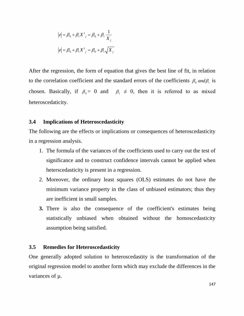
147

1

0 0

1i j i

j

e XX

1

0 0i j i je X X

After the regression, the form of equation that gives the best line of fit, in relation

to the correlation coefficient and the standard errors of the coefficients 0 iand is

chosen. Basically, if 0 = 0 and 1 ≠ 0, then it is referred to as mixed

heteroscedaticity.

3.4 Implications of Heteroscedasticity

The following are the effects or implications or consequences of heteroscedasticity

in a regression analysis.

1. The formula of the variances of the coefficients used to carry out the test of

significance and to construct confidence intervals cannot be applied when

heterscedasticity is present in a regression.

2. Moreover, the ordinary least squares (OLS) estimates do not have the

minimum variance property in the class of unbiased estimators; thus they

are inefficient in small samples.

3. There is also the consequence of the coefficient's estimates being

statistically unbiased when obtained without the homoscedasticity

assumption being satisfied.

3.5 Remedies for Heteroscedasticity

One generally adopted solution to heteroscedastity is the transformation of the

original regression model to another form which may exclude the differences in the

variances of µ.

148

This is a systematic approach which is carried out to obtain the best form of

equation in which the transformed disturbance term has constant variance.

For example given the equation

0 1 1 iY X

where i is heteroscedastic, a transformation could be done as follows

0i ii

i i i

Y

X X X

Here, i

iX

is homoscedastic

Since 2

2 2

2 2

1 1ii i

i i i

E EX X X

4.0 CONCLUSION

In this unit you have learnt what heteroscedaticity is, its causative factors, its


5.0 SUMMARY

In this unit you have learnt that heteroscedasticity is the assumption that the

variance of each random variables, µ is not the same for all values of the

explanatory variable X.

Causes of heteroscedasticity in regression are:

1. Errors in measurement of variables

2. Omission of relevant variables

3. Presence of outliers

149

4. Incorrect data transformation and incorrect functional form

The most conventional test applied to detect heteroscedasticity are:

1. the Spearman rank-correlation test and

2. the Glejser test

The effects or implications or consequences of heteroscedasticity in a regression

analysis are:

1. the formula of the variances of the coefficients cannot be applied when

heterscedasticity is present in a regression.

2. the ordinary least squares (OLS) estimates do not have the minimum

variance property in the class of unbiased estimators.

3. the consequence of the coefficient's estimates are statistically biased.

Remedies of heteroscedasticity are:

1. The transformation of the original regression model to another form.

2. Inclusion of relevant variables

3. Removal of outliers


5. Explain what you understand by heteroscedasticity as a problem in a

regression model

6. What are the causes of heteroscedasticity

7. What are the consequences of heteroscedasticity

8. What are the remedial measures of heteroscedasticity

150









Edition, South-Western Centage Learning, Mason, US

151

MODULE 6: ANALYSIS OF VARIANCE (ANOVA)

Unit 1: The Meaning and Essence of Analysis of Variance (ANOVA)

Unit 2: Types of Analysis of Variance (ANOVA)

Unit 3: Approaches to Analysis of Variance (ANOVA)

Unit 4: Interpretation of Analysis of Variance (ANOVA) Results

UNIT 1: THE MEANING AND ESSENCE OF ANALYSIS OF VARIANCE

(ANOVA)

1.0 Introduction

2.0 Objectives

3.0 Main Content

3.1 Meaning of analysis of variance (ANOVA)

3.2 The essence of analysis of variance (ANOVA)

4.0 Conclusion

5.0 Summary



1.0 INTRODUCTION

In this unit we shall explain the meaning and the essence of analysis of

variance (ANOVA).

2.0 OBJECTIVES


explain the meaning of analysis of variance (ANOVA)

know the essence of analysis of variance (ANOVA)

152

3.0 MAIN CONTENT

3.1 The meaning of and terminologies used analysis of variance (ANOVA)

Analysis of Variance (ANOVA) is a statistical tool used to detect differences between

experimental group means. ANOVA is a statistical test for detecting differences in group

means when there is one parametric dependent variable and one or more independent

(categorical) variables.

ANOVA is a statistical technique used for apportioning the variation in an observed data

into its different sources. In other words, it is a technique employed to break down the

total variation in an experiment to its additive components. With this technique or method

therefore, we can break down the total variation, occurring in a dependent variable, into

various separate factors causing the variation. ANOVA technique can be seen as a

technique which can be used to assign the total variation in an experiment to the

individual factors used in the experiment, combination of factors and /or to nature (i.e.

chance).

In adopting this technique for the analysis of data, assumptions concerning the nature of

statistical relationship between the dependent and the independent variables are not

considered or made. Rather, certain assumptions are made concerning the treatments of

the experiments. Thus, ANOVA does not stipulate any functional relationship between

the dependent and the independent variable but it enables us to break down the total

variation into the different sources or causes of the variation.

However, to understand this statistical technique clearly, certain associated

terms/terminologies need some clarifications. These include:

a. Factors: They are independent variables to be studied in an experiment. They are

variables whose effect on another variable to be studied. Example is the study of the

effect of carbohydrate on the weight gain in chicken. The factor here is carbohydrate.

153

b. Factor Levels: They are groups within each factor. They are sources of a particular

factor. Hence, in the study of the effect of carbohydrate on the weight gain in chicken, the

factor levels are the different sources of the factor (carbohydrate) under study. These

sources include; wheat, dried cassava peels, maize and others. Each of these sources is a

factor level.

c. Treatment: A treatment is equivalent to a factor level in a single-factor analysis.

However, in multi-factor analysis, a treatment is equivalent to a combination of factor

levels. For instance, in the study of the effect of carbohydrate on the weight gain in

chicken, each of the factor levels (that is wheat, dried cassava peels and maize) is a

treatment under a single-factor analysis.

In considering treatment as a combination of factor levels, consider this illustration.

Suppose we wish to study the effect of different breeds of chicken and different sources

of carbohydrates on the weight gain in chicken. We may decide to use three (3) different

breeds of chicken and three (3) sources of carbohydrate, and this will give a total of nine

(3 x 3 = 9) treatments. This is so because each of the sources of carbohydrate will

combine with each breed of chicken to form a treatment. This combination of factor

levels can be illustrated thus:

Sources of carbohydrate (FA):

1. Dried Cassava peels (C)

2. Wheat (W)

3. Maize (M)

Breeds of Chicken (FB):

1. Harco (H)

2. Nera (Hypeco)

154

3. Amo Sanders (S)

FB

FA

C W M

H HC HW HM

P PC PW PM

S SC SW SM

The treatments in this experiment are: HC, HW, HM, PC, PW, PM, SC, SW and SM

d. ANOVA Table: It is a table that shows in summary form, the computations for

analysis of variance (ANOVA). This table enables us to have a quick and convenient

assessment of the sources of variation, their respective sum of squares and degrees of

freedom which are results of ANOVA.

3.2 The Essence of ANOVA

Analysis of variance is a very important analytical tool developed by R.A. Fisher for the

analysis of experimental data. Hence, it is employed in such fields of study as agriculture,

medicine, engineering, economic and other social researches to analyze data and achieve

logical conclusions.

Besides determining the various factors which cause variation of the dependent variable,

ANOVA could also be useful in the following areas:

(i) testing the overall significance of the regression;

(ii) testing the significance of the improvement in fit obtained by the introduction of

additional explanatory variables in the function;

(iii) testing the equality of coefficients obtained from different samples;

155

(iv) testing the stability of coefficients of regression; and

(v) testing restrictions imposed on coefficient of a function.

Basically, analysis of variance technique is used to test hypothesis concerning population

means; and it is employed in regression analysis to conduct various tests of significance.

Hence, it is an essential component of any regression analysis.

4.0 CONCLUSION

In this unit you have learnt the meaning and essence of analysis of variance (ANOVA).

5.0 SUMMARY

Analysis of Variance (ANOVA) is a statistical tool used to detect differences between

experimental group means. ANOVA is a statistical test for detecting differences in group

means when there is one parametric dependent variable and one or more independent

(categorical) variables.

ANOVA is a statistical technique used for apportioning the variation in an observed data

into its different sources.

Besides determining the various factors which cause variation of the dependent variable,

ANOVA could also be useful in the following areas:

(i) testing the overall significance of the regression; (ii) testing the significance of the

improvement in fit obtained by the introduction of additional explanatory variables in the

function; (iii) testing the equality of coefficients obtained from different samples; (iv)

testing the stability of coefficients of regression; and (v) testing restrictions imposed on

coefficient of a function.


1. What do you understand by analysis of variance?

2. What makes analysis of variance to be different from t-test?

156

3. Besides determining the various factors which cause variation of the dependent

variable, where could ANOVA also be useful?





Edition,



State, Nigeria

Sawyer, S. F. (n.d.). Analysis of Variance: The Fundamental Concepts, The Journal of

Manual & Manipulative Therapy 17 (2):27-38.

157

UNIT 2: TYPES OF ANALYSIS OF VARIANCE (ANOVA)

1.0 Introduction

2.0 Objectives

3.0 Main Content

3.1 Types of analysis of variance (ANOVA)

4.0 Conclusion

5.0 Summary



1.0 INTRODUCTION

In this unit we shall explain the types of analysis of variance (ANOVA).

2.0 OBJECTIVES


types of analysis of variance (ANOVA).

3.0 MAIN CONTENT

3.1 Types of analysis of variance

Before adopting this analytical technique, we consider the number of criteria (factors) to

be studied. Based on this, ANOVA has two basic classifications or types, namely one-

way or one- factor ANOVA and two-way or two-factor ANOVA.

1. One- Factor ANOVA

In one-factor analysis of variance, there are only two variables: one dependent variable

and one independent variable. It is used to find out the effect(s) of the single independent

158

variable (factor) on the dependent variable. For instance, in the study of the level of

maize yield using different sources of phosphorus, we are considering the effect of

phosphorus on the yield of maize. Hence, phosphorus is the independent variable (factor),

while the yield of maize is dependent on it. Based on this, we adopt the one-factor

analysis of variance to determine if the variation in maize yield is due to the treatment

(phosphorus application) or due to chance.

However, to adopt and apply this one-factor ANOVA, the following assumptions must be

made:

1. The treatment effect is fixed, that is Tr is fixed.

2. The total effect of the treatment is equal to zero; that is

1

0N

ri

T

3. The sum expected value of the effect is equal to zero i.e,

1

0N

ii

4. The error is normally and independently distributed with mean zero and variance, 2

2~ (0, )N

Consider the following yield equation;

r iY T e --------------------------------(i)

Where:

Y = Yield of the crop

= Population mean

rT = Treatment effect

159

i = error effect which is due to nature, chance or any other factors which are

beyond human control.

From equation (i) above, the only factor considered to affect yield is the treatment

applied. Any variation in the yield of the crop could, therefore, be attributed to the

treatment applied to the crop or nature. The treatment applied may (or may not) cause a

significant effect on the yield. In other to arrive at a logical conclusion about the effect of

the treatment (independent variable) on the crop yield (dependent variable), we use the F-

test. With this test, therefore, we can say, with some level of confidence, whether the

treatment has a significant effect or not on crop yield.

2. Two-Factor ANOVA

Unlike the one-factor ANOVA, the two-factor classification contains more than two

variables. It is made up of one dependent variable and two independent variables

(factors). It is basically employed to determine the effects of the two independent

variables (factors) on the dependent variable. This technique, therefore, enables us to

estimate not only the separate effects of the factors (independent variables) but also the

joint effect (interaction effect) of these factors on the dependent variable.

Consider the study of the effects of fertilizer and soil type on the yield of cassava. There

are two independent variables or factors namely; fertilizer and soil type, and one

dependent variable (cassava yield). Hence, the effects of these two factors (fertilizer and

soil type) can be analyzed using the two factor analysis of variance technique.

By using this technique, the separate effect of the two factors on the yield of cassava will

be determined. Also, the combined effect (interaction effect) of the two factors on

cassava yield can be shown. However, when the two factors do not have any interaction

effect, we say that they have additive effects on the dependent variable (cassava yield).

160

In applying the two-factor analysis of variance technique, the same assumptions holding

in a one-factor technique still hold.

3.2 ANOVA Table

This is a table which presents, in summary form, the computational results of the analysis

of variance. It shows the values for the degree of freedom (df); sum of squares (SS),

Mean squares (MS) and F-ratio. This table is in two forms; one-factor ANOVA table and

two-factor ANOVA table.

One-Factor ANOVA Table

This summarizes the results for the degree of freedom (df), sum of squares (ss) and mean

squares (MS) for the total variation, treatment variation and variation due to error for

one- factor experiment. It equally presents the F- ratio value which is used for hypothesis

testing. The following is the summary of the ANOVA table for a one-factor experiment.

Table 6.1: ANOVA Table for One-Factor Experiment

Source of

Variation

Sum of

Squares (SS)

Degree

of

Freedom

(DF)

Mean Squares (MS) F-ratio

Total 2

1

N

jkjk

Y CT

N – 1 2

1

1

N

jk

jk

Y CT

N

tMean Square reatme

Mean Squaree

nt

rror

Treatment

(between

treatments)

2

1

t

jj

Y CT

t -1 2

1

1

t

j

j

Y CT

t

Residual

(Error)

(within

treatments)

SS Total – SS

Treatments

N – t SS Total SS Treatment

N t

161

Where:

CT = Correlation terms =

2

1

N

jk

jk

Y

N

r = Number of replications for treatment

t = Number of treatments

N = Total number of observations

2

1

N

jk

jk

Y

= sum of the squares of all the observation in the experiment.

2

1

t

j

j

Y

= sum of the squares of all the observations per treatment.

1

N

jk

jk

Y

= sum of all the observations in the experiment.

Two-Factor ANOVA Table

In this case, the table presents in the summary, the results for the degree of freedom sum

of squares and mean squares for the total variation, treatment variation of the two factors,

and variation due to randomness (error). Equally, the F-ratio values are evaluated and

presented in this table. The summary of a two-factor ANOVA table is shown below.

162

Table 6.2: ANOVA Table for Two- Factor Experiment

Source of

Variation

Sum of

Squares

(SS)

Degree

of

Freedom

(DF)

Mean Squares (MS) F-ratio

Total 2

N

jk

jk

X CT

N – 1 2

1

N

jk

jk

X CT

N

Treatments

(Between

Treatments)

2

1

t

j

j

X

CTb

t -1 Treatment

1

SS

t

tMS reatme

MS e

nt

rror

Block

(Between

Blocks)

2

1

b

k

k

X

CTt

b -1 Blo

1

ckSS

b

Block

MS e

MS

rror

Error

(Random)

SS Total –

(SS

Treatment +

SS Block)

(t-1)(b-1) Erro

) )

r

( 1 ( 1t

S

b

S

Where:

b = Number of blocks used

t = Number of treatments

CT = correction term

2

1

N

jk

jk

Y

N

N =Total number of observations

163

2N

jk

jk

X= Sum of the squares of all the observations in the experiment

2

1

t

j

j

X

= Sum of the squares of all observations per treatment

2

1

b

k

k

X

= Sum of the squares of all observations per block.

4.0 CONCLUSION

In this unit you have learnt about the one-factor and two-factor ANOVA and how these

two types of ANOVA tables are tabulated for easy computation of F-ratio.

5.0 SUMMARY

In this unit you have learnt that:

One-factor ANOVA has only two variables: one dependent variable and

one independent variable. It is used to find out the effect(s) of the single

independent variable (factor) on the dependent variable. For instance, in the

study of the level of maize yield using different sources of phosphorus, we

are considering the effect of phosphorus on the yield of maize. Hence,

phosphorus is the independent variable (factor), while the yield of maize is

dependent on it.

The two-factor ANOVA contains more than two variables. It is made up of

one dependent variable and two independent variables (factors). It is

basically employed to determine the effects of the two independent

variables (factors) on the dependent variable. This technique, therefore,

enables us to estimate not only the separate effects of the factors

164

(independent variables) but also the joint effect (interaction effect) of these

factors on the dependent variable.


1. What do you understand by one-factor ANOVA and two-factor ANOVA.

2. Discuss the assumptions that must hold before adopting one-factor ANOVA

3.





Edition,



State, Nigeria.

165

UNIT 3: APPROACHES FOR COMPUTING THE ANALYSIS OF VARIANCE

(ANOVA)

1.0 Introduction

2.0 Objectives

3.0 Main Content

3.1 The econometrics (regression) approach for the analysis of variance

(ANOVA)

3.2 The statistical approach for the analysis of variance (ANOVA)

4.0 Conclusion

5.0 Summary



1.0 INTRODUCTION

In this unit you shall understand the two major computational approaches for the

analysis of variance (ANOVA) namely the econometric or regression and the

statistical approaches.

2.0 OBJECTIVES


compute ANOVA using econometric/regression approach and the statistical

approach.

3.0 MAIN CONTENT

3.1 The Econometric or Regression Approach to ANOVA

Regression analysis is a tool used to determine the various causes of variations in the

dependent variable. In the course of determining the causes of the variation, it splits the

166

variation (total variation) into two, the explained and the unexplained variations. The

method of analysis of variance is then used to conduct the various tests of significance

required in the regression analysis.

In the simple regression analysis, the estimated regression equation is given by;

0 1 1ˆ ˆ ˆ

tY a a X e -------------------------(ii)

Comparing the above equation with the yield equation (i), r iY T e ,

some interesting revelations could be made thus;

Y = Y = Estimated yield

= 0a = Population means

rT = 1X = Independent factor

ie = te = Error term or error effect.

Just like in simple regression analysis, the variation in a one-factor ANOVA equation can

be broken down as follows:

expTotal Variation Explained Un lained

Varation or Variation orVariation due Variation due to natureto treatment effect or randomness

ir eTY

However, regression analysis differs from analysis of variance (ANOVA) technique.

While analysis of variance technique provides only information concerning the

breakdown of the total variation, regression analysis, in addition to this information, also

provides numerical values for the influences of various independent variables on the

dependent variable.

167

From equation (ii), the error term, et, which is the deviation of the estimated value of the

independent variable from its actual observation is given by:

î i tY Y e

Where;

iY = actual observation of the dependent variable at a particular time

îY = estimated value of the dependent variable at a particular period

te = error term

Taking the squares of both sides, we have

2 2 2î i tY Y e

By summation of the squares and rearranging the above equation, it becomes;

2 2 2î i tY Y e

Hence, we can have the following analogy;

Total sum of squares = Regression sum of squares + Error sum of squares

That is,

2

iY = Total sum of squares = Total variation.

2îY = Regression sum of squares = Explained variation

2

te = Error sum of squares = Unexplained variation.

168

It is the study of these components of the total sum of squares (SS Total) that is called

the analysis of variance from regression point of view.

More so, in regression analysis the amount of variation in the dependent variable

explained by the included independent (explanatory) variable(s) is quantified by

coefficient of determination, R². It therefore, implies that regression sum of squares is a

component of the coefficient of determination, R². This is so since the regression sum of

squares involves only the variation caused by the included independent or explanatory

variable(s), and not the variation due to error or nature.

Mathematically,

1 1 2 2 3 32

2

... n nb x y b x y b x y b x yR

y

It implied that;

Regression sum of squares (RSS) = 1 1 2 2 3 3 ... n nb x y b x y b x y b x y

and

Total sum of squares (TSS) = ∑y²

Hence,

2 RSSR

TSS

The ANOVA table for the computational procedures, to determine the sources of

variation in the dependent variable caused by n-independent variables (factors) can be

shown thus;

169

Table 6.3: ANOVA Table for n-independent Variables

Source of

Variation

Sum of Squares Df Mean

Squares

F-ratio

Explained

(By included

explanatory

varaibales)

1 1 2 2 3 3 ... n nb x y b x y b x y b x y K-1

1

RSS

K ( 1)

RSSK

ESSN K

Unexplained

(Due to

nature or

error)

2

ie ESS N-

K

ESS

N K

Total 2

iy SST N-1

1

SST

N

Worked Example: In the study of the effect of the period of storage on the moisture

content of yam, the following data were obtained:

Moisture content, Y

60

57

50

41

30

19

Period of storage, X

1

2

5

10

15

21

Calculate the explained and unexplained variation in the moisture content of yam, and

test the overall significance of the regression at 99% level of confidence.

Solution:

Step 1: Estimate the regression coefficients.

0 1 tY b b X e

170

1 2ˆ xyb

x

and 0 1ˆ ˆb Y b X

Table 6.4: Obtaining Data for estimating regression coefficients 0b and 1b .

Y X ix X X

9ix X

iy Y Y

42.83iy Y

xy x2

y2

60 1 1-9 = -8 60-42.83 = 17.17 -8x17.17 = -37.36 (-8)2= 64 (17.17)

2= 194.81

57 2 2-9 = -7 57 – 42.83 =14.17 -7 x 14.17 = -9.19 (-7)2= 49 (14.17)

2= 200.79

50 5 5-9 = -4 50 – 42.83 = 7.17 -4 x 7.17 = -28.68 (-4)2= 16 (7.17)

2 = 51.41

41 10 10-9 = 1 41 – 42.83 = -1.83 1 x -1.83 = -1.83 (1)2 = 1 (-1.83)

2 = 3.35

30 15 15-9 = 6 30– 42.83 = -12.83 6 x -12.83= -76.98 (6)2 = 36 (-12.83)

2=164.61

19 21 21-9 = 12 19 -42.83 = -23.83 12x-23.83=-285.96 (12)2=144 (-23.83)

2=567.87

ƩY=

257

ƩX=

54

Ʃxy = -630 Ʃx2 = 310 Ʃy

2 = 1282.84

N = 6

25742.83

6

YY

N

549.00

6

XX

N

1 2

630ˆ 2.03310

xyb

x

0 1ˆ ˆ 42.83 ( 2.03)(9) 42.83 19.25

61.10

b Y b X

Hence, the estimated regression equation becomes:

171

1ˆ 61.10 2.03 tY X e

Table 6.5: Analysis of Variance (ANOVA) Table

Source of

Variation

Sum of Squares Degree of

Freedom

Mean Squares F-ratio

Total Ʃy2 = 1282.84 N-1

6-1 = 5

1278.901298.4

0.985

with 1 and 4

df Explained

1 1 ( 2.03)( 630) 128.90b x y

K-1

2-1 =1

1278.901278.90

1

Unexplained 2 2

1 1 3.94i ie y b x y N-K

6-2 = 4

3.940.985

4

At 99% confidence level means 1% level of significance, and 1and 4df the F-tab = 21.2

Since F-cal > F-tab i.e. 1298.4 >21.2, we reject the null hypothesis, H0 and accept the

alternative hypothesis, Ha which states that the regression is significant.

3.2 The statistical approach for the analysis of variance (ANOVA)

In this approach, model estimation is not necessary as it is the case in the econometric or

regression approach. Rather an important estimation is the determination of the correction

term (CT).

For a one-factor ANOVA, the following must be determined as a basis for further

calculations: Sum of squares treatment (SSTr); error sum of squares (ESS) and the

degrees of freedom (df).

172

Worked Example: In a study to determine the effect of nitrogen on the yield in kg of a

certain variety of maize. The following data were obtained.

Ammonium Sulphate Urea NPK

15 13 21

24 17 18

22 25 27

19 20 32

Is there any significant difference between the yields due to the treatments (ammonium

sulphate, Urea and NPK) given or if the difference in yield is due to chance?

Solution:

Looking at this study, it is clear that there is just one-factor consider to be affecting the

yield of the maize variety.

This factor is nitrogen (as stated in the quaetion) and it has (3) factor levels, namely;

ammonium sulphate, urea and NPK.

Based on the above reasons, the one-factor ANOVA technique will be adopted in

solving the problem.

Let the factor levels be represented by A, B and C for ammonium sulphate, urea and NPK

respectively.

173

Table 6.6: Data for Computing the ANOVA

Treatment Treatment

Total (Tr) Mean, Xt

A 15 24 22 19 15+24+22+19 = 80 80/4 = 20

B 13 17 25 20 13=17+25+20 = 75 75/4 = 18.75

C 21 18 27 32 21+18+27+32 = 98 98/4 = 24.50

Grand Total = 1

N

t

i

T

i.e. sum of all the treatment totals.

= 80 + 75 + 98 =253.

Grand mean, 1

n

t

i

X

Xn

i.e. sum of the treatment means divided by total number

of treatments.

20 18.75 24.50

3X

= 21.08

NB: There are three (3) treatments and four (4)replications for each treatment. Therefore,

there are (3×4) = 12 replications in the experiment.

That is, N=3×4=12

To calculate:

174

(1) Correction term CT =

2

1

N

jk

jk

Y

N

=

2(253)

12

CT = 5334.08.

(2) Sum of Squares Total (SS Total) = (15)2 + (24)

2 + (22)

2 + (19)

2 + (13)

2 + (17)

2

+ (25)2 + (20)

2 + (21)

2 + (18)

2 + (27)

2 + (32)

2 - CT

= (225+ 576 +484+ 361+169+289+625+400+441+324+729+1024) - CT

SS Total= 5647-5334.08

SS Total = 312.92

(3) Sum of Square Treatment, SSTr =

2 2 2(80) (75) (98)

4 4 4CT

= 6400 5625 9604

5334.084 4 4

= 6400 5625 9604

5334.084

= 21629

5334.084

=5407.25 5334.08

SSTr = 73.17

(4) Error Sum of Squares (SSE) = SS Total – SSTr

= 312.92 - 73.17

SSE = 239.75

(5) (a) Degree of freedom for treatment (i.e. between treatment)

= K - 1 = 3 – 1 =2

175

(b) Degree of freedom for residual (i.e. within treatments)

= N – K =12 -3 = 9

(c) Degree of freedom for total = N – 1 = 12 -1 =11

(6) Treatment Mean Square (MSTr) = Sumof Square Treattment

Degree of Freedom

MSTr = 73.13

2= 36.59

(7) Error Mean Square (MSE) = Error Sumof Square

Degree of Freedom Error=

239.75

9

MSE = 26.64

(8) F-ratio = MSTr

MSE =

36.59

26.64 = 1.37

The above result can be presented in a one-factor ANOVA table thus:

Table 6.7: ANOVA Table for Effect of Nitrogen on Maize Y

Source of

Variation

Sum of Squares Degree of

Freedom

Mean Squares F-ratio

Treatment 73.17 2 36.59 36.591.37

26.64

with 2 and

9 df

Residual

(Error)

239.75 9 26.64

Total 312.92 11 28.45

The mean squares are not additives while the sum of squares is additives. From the above

table, SSTr +SSE = SS Total (73.17 +239.75 =312.92) but MSTr +MSE ≠ MST (36.59

+26.64 ≠28.45)

Conclusion:

176

In order to make our conclusion based on the hypothesis made, we need to compare the

F-cal with the F-tab at a given level of significance and degree of freedom, df 2 and 9.

Using 5% level of significance, and 2 and 9 df, we have that;

F-tab = 4.26 (From the theoretical F-table)

Since F-cal < F-tab i.e., 1.37< 4.26, we conclude that on the average, there are no

significant difference among the treatments i.e., we accept H0 and reject Ha.

However, it is important to note that this does not readily prove that there is no difference

among the treatments. It could be that some treatment difference exists but the

experiment was not sensitive enough to detect those differences at the level of probability

or significance used.

Worked Example: A soil scientist wishes to assess the effect of difference source of

ashes and organic manure on the PH level of some soil samples. During the experiment,

the following data were generated.

Table 6.8a:

Factor B Factor B

Ash

(organic manure) Ai Aii Aiii

OM 1 7.9 12.0 10.5

OM 2 13.0 6.5 8.1

OM 3 8.9 5.2 11.0

OM 4 13.0 11.2 9.3

Determine at 5% significance level whether there is a difference in PH per sample: (a)

due to the organic manures (b) due to the ashes.

177

Solution:

Table 6.8b: Data to obtain the ANOVA using Statistical Approach

Factor B

Factor B i ii iii Row total Row Mean

OM 1 7.9 12.0 10.5 30.4 30.4/4 = 10.13

OM 2 13.0 6.5 8.1 27.6 27.6/4 = 9.20

OM 3 8.9 5.2 11.0 25.1 25.1/4 = 8.37

OM 4 13.0 11.2 9.3 33.5 33.5/4 = 11.17

Column total 42.8 34.9 38.9

Column mean 42.8/4 = 10.7 34.9/4 = 8.73 38.9/4 = 9.73

Grand total = (7.9 +12.0 +10.5 +13.0 +6.5+8.1+ 8.9 + 5.2+ 11.0+13.0+11.2 +9.3) =

116.6

Grand mean = 10.7 8.73 9.73

3

=

29.16

3 = 9.72

To calculate:

(i) Correction Term, CT =

2

1

N

jk

jk

Y

N

=

2(116.6)

12

= 1132.96

(ii) Sum of Square Total (SS Total) = 2

1

N

jk

jk

X CT

SS Total = (7.9)2 + (12.0)

2 +(10.5)

2 +(13.0)

2 + (6.5)

2 + (8.1)

2 + (8.9)

2 + (5.2)

2 + (11.0)

2

+

(13.0)2 + (11.2)

2 + (9.3)

2 - CT.

SS Total = 1201.7 – CT

= 1201.7 - 1132.96

178

SS Total = 68.74

(iii) Sum of squares treatments (SS Treatment) =

2

1

t

j

j

X

CTb

SS Treatment =

2 2 2 2(30.4) (27.6) (25.1) (33.5)1132.96

3

SS Treatment 1146.06 - 1132.96 = 13.10

(iv) Sum of square block (SSB) =

2

1

b

k

k

X

CTt

SSB = 2 2 2(42.8) (34.9) (38.9)

1132.964

SSB = 1140.77 - 1132.96 = 7.81

(v) Error sums of squares = SS Total - (SS Treatment + SSB)

= 68.74 - (13.10 +7.81) = 68.74 -20.91

SSE = 47.83

(vi) (a) Degree of freedom for treatment = t -1 = 4 -1 =3

(b) Degree of freedom for block = b -1 = 3 -1 = 2

(c) Degree of freedom for error = (t-1)(b-1) = (3×2) = 6

(d) Degree of freedom for total = N – 1 = 12 -1 =11

(vii) Treatment mean squares (MS Treatment)

= Treatment

1

SS

t =

13.10

3 = 4.37

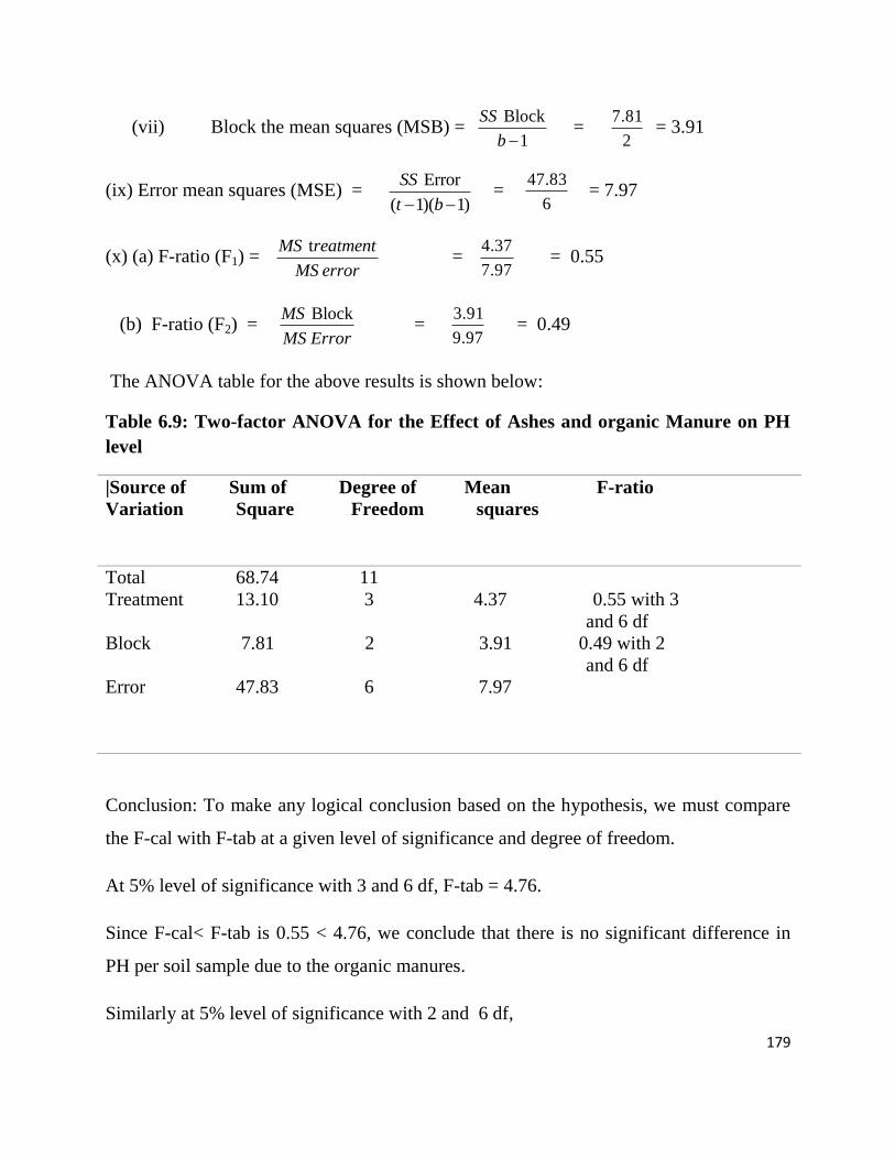
179

(vii) Block the mean squares (MSB) = Blo

1

ckSS

b =

7.81

2 = 3.91

(ix) Error mean squares (MSE) = Erro

) )

r

( 1 ( 1t

S

b

S

=

47.83

6 = 7.97

(x) (a) F-ratio (F1) = tMS reatme

MS e

nt

rror =

4.37

7.97 = 0.55

(b) F-ratio (F2) = Block

MS E

MS

rror =

3.91

9.97 = 0.49

The ANOVA table for the above results is shown below:

Table 6.9: Two-factor ANOVA for the Effect of Ashes and organic Manure on PH

level

|Source of Sum of Degree of Mean F-ratio

Variation Square Freedom squares

Total 68.74 11

Treatment 13.10 3 4.37 0.55 with 3

and 6 df

Block 7.81 2 3.91 0.49 with 2

and 6 df

Error 47.83 6 7.97

Conclusion: To make any logical conclusion based on the hypothesis, we must compare

the F-cal with F-tab at a given level of significance and degree of freedom.

At 5% level of significance with 3 and 6 df, F-tab = 4.76.

Since F-cal< F-tab is 0.55 < 4.76, we conclude that there is no significant difference in

PH per soil sample due to the organic manures.

Similarly at 5% level of significance with 2 and 6 df,

180

F-tab = 5.14. Since F cal < F tab i.e. 0.49 < 5.14, we also conclude that there is no

significant difference in PH per soil samples due to ashes. Hence, we accept H0 and reject

Ha in both cases.

4.0 CONCLUSION

In this unit you have leant the two major computational approaches for the analysis of

variance (ANOVA) namely the econometric or regression and the statistical approaches.

5.0 SUMMARY

In this unit you have learnt:

regression analysis differs from analysis of variance (ANOVA) technique.

While analysis of variance technique provides only information concerning

the breakdown of the total variation, regression analysis, in addition to this

information, also provides numerical values for the influences of various

independent variables on the dependent variable.

in regression analysis the amount of variation in the dependent variable

explained by the included independent (explanatory) variable(s) is

quantified by coefficient of determination, R². It therefore, implies that

regression sum of squares is a component of the coefficient of

determination, R². This is so since the regression sum of squares involves

only the variation caused by the included independent or explanatory

variable(s), and not the variation due to error or nature.


1. Two varieties of oil palm is processed by cottage industries and stored for the

period of ten months. Test whether the storage period affects the quality of the

palm oil from the two varieties.

181

Months 1 2 3 4 5 6 7 8 9 10

A 32 30 35 33 35 34 29 32 36 34

B 35 38 37 40 41 35 37 41 36 40

2. In a survey conducted by the National Bureau of Statistics (NBS) to examine the

consumption of LAKE, EBONYI, and OFADA brands of local rice. It collects a

sample of three for each of the treatments (rice brands). Using the hypothetical

data provided below, test whether the mean consumption test is equal for each

brand of rice. Use 5% level of significance (α =5%).

LAKE EBONYI OFADA

643 466 484

655 427 456

702 525 402

3. An agribusiness firm wishes to compare four programmes for training workers to

perform a certain manual task. Twenty new employees are randomly assigned to

the training programmes, with 5 in each programme. At the end of the training

period, a test is conducted to see how quickly trainees can perform the task. The

number of times the task is performed per minute is recorded for each trainee. Use

5% level of significance (α =5%) to test whether the training affects the task

performed.

Programme 1 Programme 2 Programme 3 Programme 4

9 10 12 9

12 6 14 8

14 9 11 11

11 9 13 7

13 10 11 8

182





Edition,







State, Nigeria.

183

UNIT 4: INTERPRETATIONS OF ANOVA RESULTS

1.0 Introduction

2.0 Objectives

3.0 Main Content

3.1 The interpretations of ANOVA results

4.0 Conclusion

5.0 Summary



1.0 INTRODUCTION

In this unit you shall understand the interpretations of analysis of variance (ANOVA)

results for policy making.

2.0 OBJECTIVES


interpret analysis of variance (ANOVA) results

3.0 MAIN CONTENT

3.1 The interpretation of analysis of variance (ANOVA) results

The objective of ANOVA is to split the total variation into its various components, and

then draw inferences on the significance of the effect of the sources or causes (ie factors)

of the variation we are considering.

In order to do this, the following procedure must be followed:

1. Set up an hypothesis

Set a null hypothesis (H0) that the treatment is not significant i.e., H0: Tr = 0.

184

Also set an alternative hypothesis that the treatment effect is significant i.e., Ha: Tr

≠ 0.

2. Choose (if not given) the level of significance and find the tabulated (theoretical)

F-ratio from the table at a specific degree of freedom (df).

3. Compare the tabulated F-ratio (F-tab) with calculated f-ratio (F-cal).

4. Make the conclusion based on the result of the comparison.

If F-cal< F-tab, Accept H0 and Reject Ha

If F-cal > F-tab, Accept Ha and Reject H0

Worked Example: Four tropical feedstuffs were each fed to a batch of chicks. The mean

daily weight gains of the chicks were as presented below:

Chicks

Batch C1 C2 C3 C4 C5

1 55 49 42 21 52

2 61 112 30 89 63

3 42 97 81 95 92

4 169 137 169 85 154

Make use of the above table to analyse the variance and test the quality of the batches for

effect on weight gain.

185

Solution:

Table 4.1:

Batch Treatment

Treatment

(Feedstuffs)

C1 C2 C3 C4 C5 Total (Tt) Means

1 55 49 42 21 52 215 43

2 61 112 30 89 63 355 71

3 42 97 81 95 92 407 81.4

4 169 137 169 85 154 714 142.8

Batch Total 323 395 322 290 361

Grand Total = 1

N

t

Tt

= 215 + 355 + 407 + 714 =1691

Total observations, N = 20

(i) Correction term = 2(1691) 2859481

142974.0520 20

(ii) SS Total = 181021 - 142974.05

= 38046.95

(iii) SS Treatment = 169539 - 142974.05

= 26564.95

(iv) SS Block (Batch) = 144614.74 - 142974.05

= 1640.7

(v) SS Error = SS Total – (SS Treatment + SS Block)

= 38046.95 – (26564.95 + 1640.70)

= 9841.3

(vi) DF for treatment = 4 – 1 = 3

DF for block = 5 - 1 = 4

186

DF for error = 3×4 = 12

(vii) MS Treatment = 26564.95

8854.983

MS Block = 1640.7

410.184

MS Error =

9841.3820.11

12

(viii) F-ratio (Treatment) = 8854.98

10.80820.11

F-ratio (Block) = 410.18

0.500820.11

The ANOVA Table for the above calculations is shown below:

Source of

Variation

Sum of

Squares

Df Mean Squares F-ratio

Total 38046.95

Treatment 26564.95 3 8854.98 10.80 with 3

and 12 df

Block 1640.70 4 40.18 0.50 with 4

and 12 df

Error 9841.3 12 820.11

At 5% significance level, with 4 and 12 df, the F-tab = 3.49. Since F-cal < F tab i.e. 0.50

< 3.49, we reject the alternative hypothesis, Ha and accept the null hypothesis, H0. The

null hypothesis states that the quality of the batches has no significant effect on weight

gain.

187

4.0 CONCLUSION

In this unit you have understood the interpretations of analysis of variance (ANOVA)

results for policy making.

5.0 SUMMARY

The objective of ANOVA is to split the total variation into its various components, and

then draw inferences on the significance of the effect of the sources or causes (ie factors)

of the variation we are considering.

In order to do this, the following procedure must be followed:

1. Set up an hypothesis

Set a null hypothesis (H0) that the treatment is not significant i.e., H0: Tr = 0.

Also set an alternative hypothesis that the treatment effect is significant i.e., Ha: Tr

≠ 0.

2. Choose (if not given) the level of significance and find the tabulated (theoretical)

F-ratio from the table at a specific degree of freedom (df).

3. Compare the tabulated F-ratio (F-tab) with calculated f-ratio (F-cal).

4. Make the conclusion based on the result of the comparison.

If F-cal< F-tab, Accept H0 and Reject Ha

If F-cal > F-tab, Accept Ha and Reject H0


1. Three different brands of magnetron tubes (the key component in microwave

ovens) were subjected to stress testing. The number of hours each operated before

needing repair was recorded.

188

Brand

A 36 48 5 67 53

B 49 33 60 2 55

C 71 31 140 59 224

Test the hypothesis that the mean lifetime under stress is the same for the three brands at

5 % level of significance.

2. Four treatments for fever blisters, including a placebo (A), were randomly

assigned to 20 patients. The data below show, for each treatment, the numbers of

days from initial appearance of the blisters until healing is complete.

Treatment Numbers of days

A 5 8 7 7 5

B 4 6 6 3 5

C 6 4 4 5 4

D 7 4 6 6 5

Test the hypothesis, at the 5% significance level, that there is no difference

between the four treatments with respect to mean time of healing.




189


Edition,



State, Nigeria.

Sawyer, S. F. (n.d.). Analysis of Variance: The Fundamental Concepts, The Journal of

Manual & Manipulative Therapy 17 (2):27-38.

aea 505: econometrics department of agricultural …

Documents