IAPWS AN5-13(2016)

The International Association for the Properties of Water and Steam

London, United Kingdom September 2013

Advisory Note No. 5:

Industrial Calculation of the Thermodynamic Properties of Seawater

2013 International Association for the Properties of Water and Steam Publication in whole or in part is allowed in all countries provided that attribution is given to the

International Association for the Properties of Water and Steam

Please cite as: International Association for the Properties of Water and Steam, Advisory Note No. 5: Industrial Calculation of the Thermodynamic Properties of Seawater (2013).

This Advisory Note has been authorized by the International Association for the Properties of Water and Steam (IAPWS) at its meeting in London, United Kingdom, 1–6 September, 2013. The Members of IAPWS are: Britain and Ireland, Canada, the Czech Republic, Germany, Japan, Russia, Scandinavia (Denmark, Finland, Norway, Sweden), and the United States, plus Associate Members Argentina and Brazil, Australia, France, Greece, New Zealand, and Switzerland. The President at the time of adoption of this document was Professor Tamara Petrova of Russia.

Summary

The calculation procedure for the thermodynamic properties of seawater for industrial use provided in this Advisory Note is based on the IAPWS Formulation 2008 for the Thermodynamic Properties of Seawater [2]. For calculating the pure water contribution, the IAPWS Formulation 1995 for the Thermodynamic Properties of Ordinary Water Substance for General and Scientific Use [5] is replaced here by the IAPWS Industrial Formulation 1997 for the Thermodynamic Properties of Water and Steam [7]. For seawater in contact with ice, the Revised IAPWS Release on an Equation of State 2006 for H2O Ice Ih [11] is used. Further details about the formulation can be found in the article by H.-J. Kretzschmar et al. [1]. Minor editorial changes were made in 2016 to correct the last digits in a few calculated values in Table A1 and to update some references.

This Advisory Note contains 24 pages, including this cover page.

Further information about this Advisory Note and other documents issued by IAPWS can be obtained from the Executive Secretary of IAPWS (Dr. R.B. Dooley, bdooley@structint.com) or from http://www.iapws.org.

2

Contents

1. Nomenclature 3 2. Introductory Remarks 5 3. Thermodynamic Properties of Seawater 6

3.1 The Fundamental Equation of State for Seawater 6

3.2 Water Part 8

3.3 Saline Part 9

4. Colligative Properties 9 4.1 Phase Equilibrium between Seawater and Water Vapor 9

4.2 Phase Equilibrium between Seawater and Ice 11

4.3 Triple-Point Temperatures and Pressures 11

4.4 Osmotic Pressure 12

4.5 Properties of Brine-Vapor Mixture 12

4.6 Properties of Brine-Ice Mixture 13

5. Reference States 14 6. Range of Validity 14 7. Uncertainty 15 8. Computing Time for the IAPWS Seawater Functions 15 9. Computer-Program Verification 17 10. References 17 APPENDIX 19

3

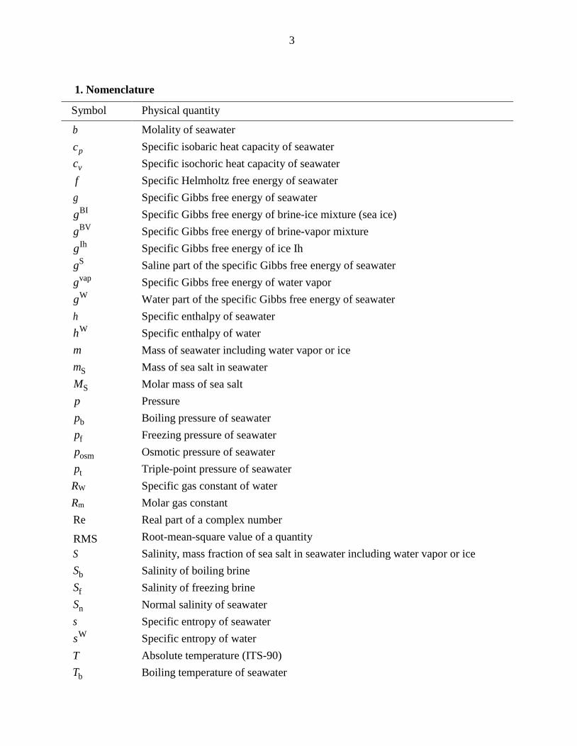
1. Nomenclature

Symbol Physical quantity

b Molality of seawater

pc Specific isobaric heat capacity of seawater

vc Specific isochoric heat capacity of seawater f Specific Helmholtz free energy of seawater g Specific Gibbs free energy of seawater

BIg Specific Gibbs free energy of brine-ice mixture (sea ice) BVg Specific Gibbs free energy of brine-vapor mixture Ihg Specific Gibbs free energy of ice Ih Sg Saline part of the specific Gibbs free energy of seawater vapg Specific Gibbs free energy of water vapor Wg Water part of the specific Gibbs free energy of seawater

h Specific enthalpy of seawater Wh Specific enthalpy of water

m Mass of seawater including water vapor or ice

Sm Mass of sea salt in seawater

SM Molar mass of sea salt p Pressure

bp Boiling pressure of seawater

fp Freezing pressure of seawater

osmp Osmotic pressure of seawater

tp Triple-point pressure of seawater RW Specific gas constant of water Rm Molar gas constant Re Real part of a complex number

RMS Root-mean-square value of a quantity S Salinity, mass fraction of sea salt in seawater including water vapor or ice

bS Salinity of boiling brine

fS Salinity of freezing brine

nS Normal salinity of seawater s Specific entropy of seawater

Ws Specific entropy of water T Absolute temperature (ITS-90)

bT Boiling temperature of seawater

4

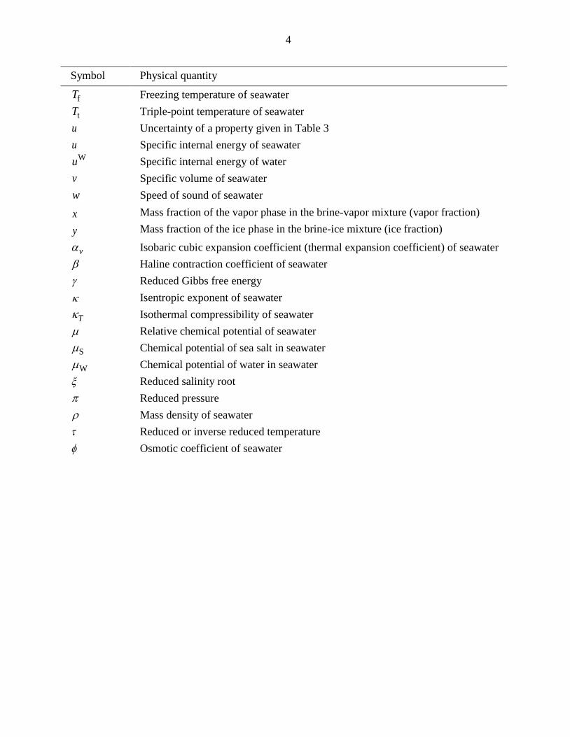
Symbol Physical quantity

fT Freezing temperature of seawater

tT Triple-point temperature of seawater u Uncertainty of a property given in Table 3 u Specific internal energy of seawater

Wu Specific internal energy of water v Specific volume of seawater w Speed of sound of seawater

x Mass fraction of the vapor phase in the brine-vapor mixture (vapor fraction) y Mass fraction of the ice phase in the brine-ice mixture (ice fraction)

vα Isobaric cubic expansion coefficient (thermal expansion coefficient) of seawater β Haline contraction coefficient of seawater γ Reduced Gibbs free energy κ Isentropic exponent of seawater

Tκ Isothermal compressibility of seawater µ Relative chemical potential of seawater

Sµ Chemical potential of sea salt in seawater

Wµ Chemical potential of water in seawater ξ Reduced salinity root π Reduced pressure ρ Mass density of seawater τ Reduced or inverse reduced temperature φ Osmotic coefficient of seawater

5

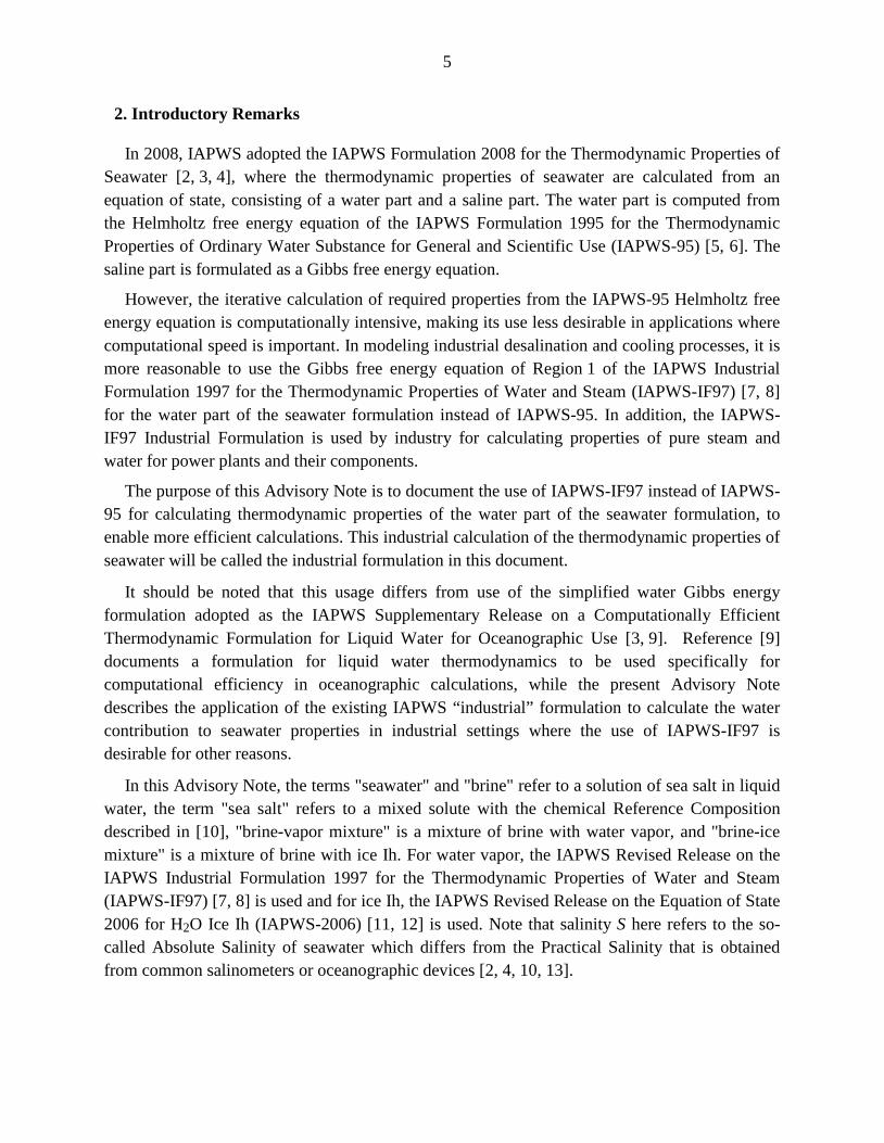
2. Introductory Remarks

In 2008, IAPWS adopted the IAPWS Formulation 2008 for the Thermodynamic Properties of Seawater [2, 3, 4], where the thermodynamic properties of seawater are calculated from an equation of state, consisting of a water part and a saline part. The water part is computed from the Helmholtz free energy equation of the IAPWS Formulation 1995 for the Thermodynamic Properties of Ordinary Water Substance for General and Scientific Use (IAPWS-95) [5, 6]. The saline part is formulated as a Gibbs free energy equation.

However, the iterative calculation of required properties from the IAPWS-95 Helmholtz free energy equation is computationally intensive, making its use less desirable in applications where computational speed is important. In modeling industrial desalination and cooling processes, it is more reasonable to use the Gibbs free energy equation of Region 1 of the IAPWS Industrial Formulation 1997 for the Thermodynamic Properties of Water and Steam (IAPWS-IF97) [7, 8] for the water part of the seawater formulation instead of IAPWS-95. In addition, the IAPWS-IF97 Industrial Formulation is used by industry for calculating properties of pure steam and water for power plants and their components.

The purpose of this Advisory Note is to document the use of IAPWS-IF97 instead of IAPWS-95 for calculating thermodynamic properties of the water part of the seawater formulation, to enable more efficient calculations. This industrial calculation of the thermodynamic properties of seawater will be called the industrial formulation in this document.

It should be noted that this usage differs from use of the simplified water Gibbs energy formulation adopted as the IAPWS Supplementary Release on a Computationally Efficient Thermodynamic Formulation for Liquid Water for Oceanographic Use [3, 9]. Reference [9] documents a formulation for liquid water thermodynamics to be used specifically for computational efficiency in oceanographic calculations, while the present Advisory Note describes the application of the existing IAPWS “industrial” formulation to calculate the water contribution to seawater properties in industrial settings where the use of IAPWS-IF97 is desirable for other reasons.

In this Advisory Note, the terms "seawater" and "brine" refer to a solution of sea salt in liquid water, the term "sea salt" refers to a mixed solute with the chemical Reference Composition described in [10], "brine-vapor mixture" is a mixture of brine with water vapor, and "brine-ice mixture" is a mixture of brine with ice Ih. For water vapor, the IAPWS Revised Release on the IAPWS Industrial Formulation 1997 for the Thermodynamic Properties of Water and Steam (IAPWS-IF97) [7, 8] is used and for ice Ih, the IAPWS Revised Release on the Equation of State 2006 for H2O Ice Ih (IAPWS-2006) [11, 12] is used. Note that salinity S here refers to the so-called Absolute Salinity of seawater which differs from the Practical Salinity that is obtained from common salinometers or oceanographic devices [2, 4, 10, 13].

6

The IAPWS Releases [2, 7, 11] referred to in this Advisory Note are available at the IAPWS website http://www.iapws.org. All details of the equations and algorithms should be taken from those Releases.

3. Thermodynamic Properties of Seawater

3.1 The Fundamental Equation of State for Seawater

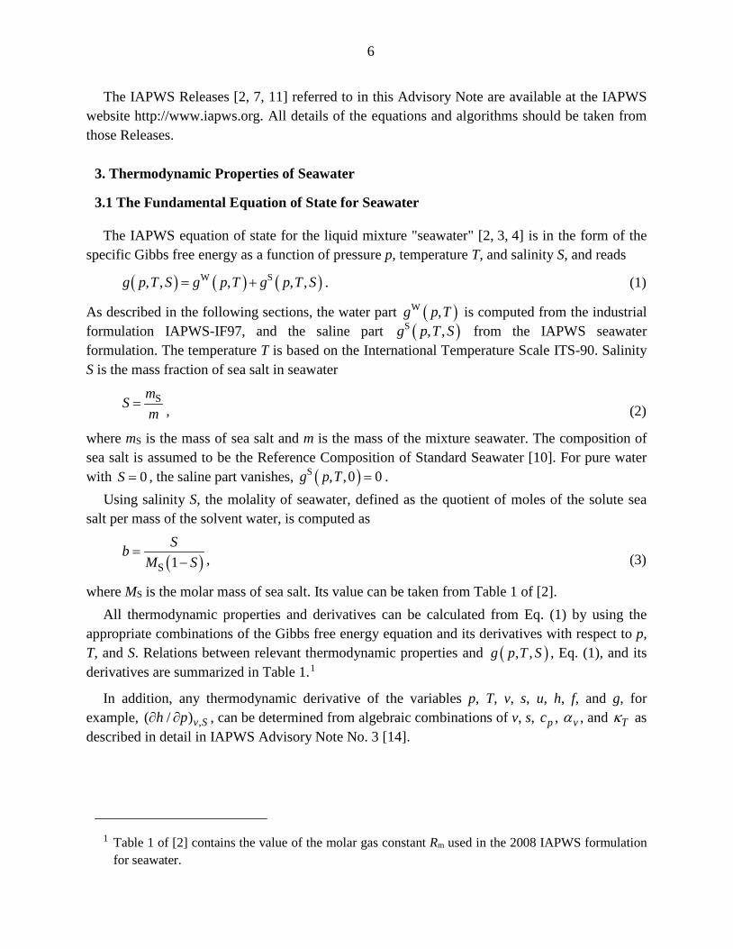
The IAPWS equation of state for the liquid mixture "seawater" [2, 3, 4] is in the form of the specific Gibbs free energy as a function of pressure p, temperature T, and salinity S, and reads

( ) ( ) ( )W S, , , , ,g p T S g p T g p T S= + . (1)

As described in the following sections, the water part ( )W ,g p T is computed from the industrial formulation IAPWS-IF97, and the saline part ( )S , ,g p T S from the IAPWS seawater formulation. The temperature T is based on the International Temperature Scale ITS-90. Salinity S is the mass fraction of sea salt in seawater

SmSm

= , (2)

where mS is the mass of sea salt and m is the mass of the mixture seawater. The composition of sea salt is assumed to be the Reference Composition of Standard Seawater [10]. For pure water with 0S = , the saline part vanishes, ( )S , ,0 0g p T = .

Using salinity S, the molality of seawater, defined as the quotient of moles of the solute sea salt per mass of the solvent water, is computed as

( )S 1Sb

M S=

− , (3)

where MS is the molar mass of sea salt. Its value can be taken from Table 1 of [2]. All thermodynamic properties and derivatives can be calculated from Eq. (1) by using the

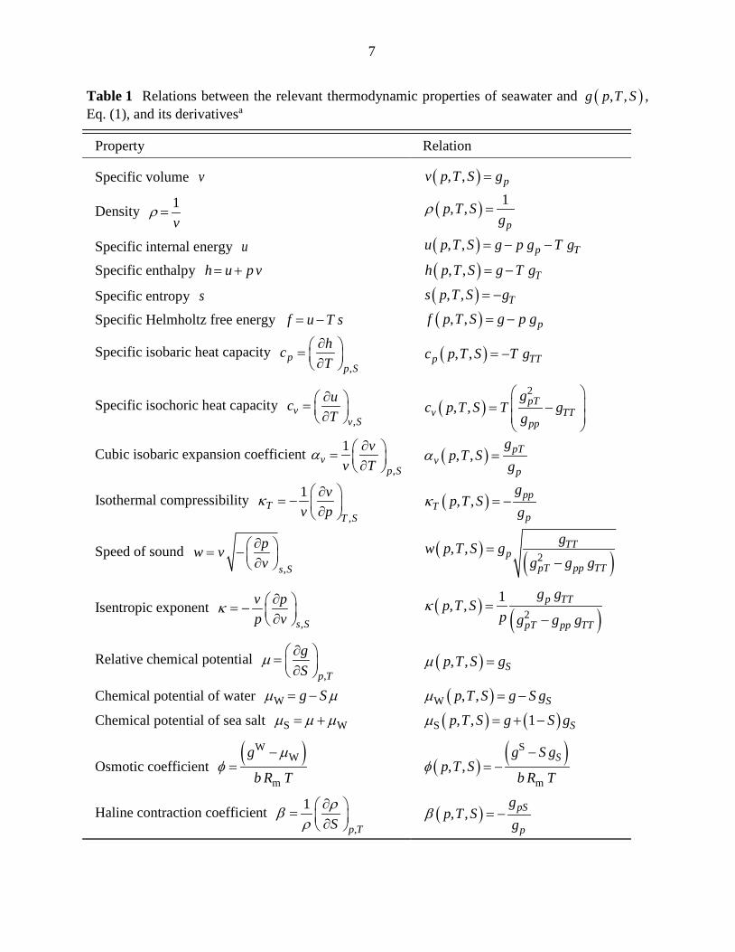
appropriate combinations of the Gibbs free energy equation and its derivatives with respect to p, T, and S. Relations between relevant thermodynamic properties and ( ), ,g p T S , Eq. (1), and its derivatives are summarized in Table 1.1

In addition, any thermodynamic derivative of the variables p, T, v, s, u, h, f, and g, for example, ,( / )v Sh p∂ ∂ , can be determined from algebraic combinations of v, s, pc , vα , and Tκ as described in detail in IAPWS Advisory Note No. 3 [14].

1 Table 1 of [2] contains the value of the molar gas constant Rm used in the 2008 IAPWS formulation

for seawater.

7

Table 1 Relations between the relevant thermodynamic properties of seawater and ( ), ,g p T S , Eq. (1), and its derivativesa

Property Relation

Specific volume v ( ) =, , pv p T S g

Density ρ = 1v

( )ρ =1, ,p

p T Sg

Specific internal energy u ( ) = − −, , p Tu p T S g p g T g

Specific enthalpy = +h u p v ( ) = −, , Th p T S g T g

Specific entropy s ( ) = −, , Ts p T S g

Specific Helmholtz free energy = −f u T s ( ) = −, , pf p T S g p g

Specific isobaric heat capacity ,

pp S

hcT∂ = ∂

( ) = −, ,p TTc p T S T g

Specific isochoric heat capacity ,

vv S

ucT∂ = ∂

( ) = −

2

, , pTv TT

pp

gc p T S T g

g

Cubic isobaric expansion coefficient ,

1v

p S

vv T

α ∂ = ∂ ( )α =, , pT

vp

gp T S

g

Isothermal compressibility ,

1T

T S

vv p

κ ∂= − ∂

( )κ = −, , ppT

p

gp T S

g

Speed of sound ,s S

pw vv∂ = − ∂

( ) ( )=

−2, , TT

ppT pp TT

gw p T S gg g g

Isentropic exponent ,s S

v pp v

κ ∂ = − ∂ ( ) ( )

κ =−2

1, , p TT

pT pp TT

g gp T S

p g g g

Relative chemical potential µ ∂ = ∂ ,p T

gS

( )µ =, , Sp T S g

Chemical potential of water µ µ= −W g S ( )µ = −W , , Sp T S g S g

Chemical potential of sea salt µ µ µ= +S W ( ) ( )µ = + −S , , 1 Sp T S g S g

Osmotic coefficient ( )µ

φ−

=W

W

m

g

b R T ( )

( )φ

−= −

S

m, ,

Sg S gp T S

b R T

Haline contraction coefficient ρβρ

∂ = ∂ ,

1

p TS ( )β = −, , pS

p

gp T S

g

8

a Definitions of derivatives used in Table 1:

∂ ∂ ∂

= = + ∂ ∂ ∂

W S

, ,p

T S T T S

g g ggp p p

, ∂ ∂ ∂

= = + ∂ ∂ ∂

2 2 W 2 S

2 2 2, ,

ppT S T T S

g g ggp p p

,

∂ ∂ ∂= = + ∂ ∂ ∂

W S

, ,T

p S p p S

g g ggT T T

, ∂ ∂ ∂

= = + ∂ ∂ ∂

2 2 W 2 S

2 2 2, ,

TTp S p p S

g g ggT T T

,

∂ ∂ ∂= = + ∂ ∂ ∂ ∂ ∂ ∂

2 2 W 2 S

pTS S

g g ggp T p T p T

, ∂ ∂ = = ∂ ∂

S

, ,S

p T p T

g ggS S

,

∂ ∂= = ∂ ∂ ∂ ∂

2 2 S

pST T

g ggp S p S

Backward functions are calculated by iteration from equations listed in Table 1. For example, for given pressure p, specific enthalpy h, and salinity S, the temperature T is calculated from the equation for ( , , )h p T S by iteration.

3.2 Water Part

The water part of Eq. (1) is calculated from the specific Gibbs free energy equation of IAPWS-IF97 region 1

( ) ( ) ( )W 34

W 1

( , ) , 7.1 1.222 ,i iI Ji

i

g p T nR T

γ π τ π τ=

= = − −∑ (4)

where the reduced Gibbs free energy is γ = W/ ( )g R T , the reduced pressure is π = / *p p and the inverse reduced temperature is τ = * /T T . The specific gas constant RW of water, the reducing parameters *p and *T , the coefficients in and the exponents iI and iJ are given in Section 5.1 of the IAPWS-IF97 Release [7].

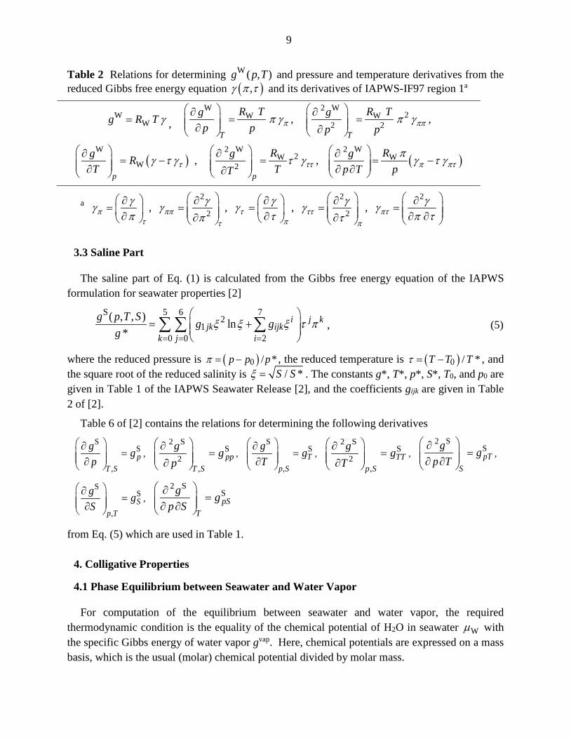
Table 2 contains the relations for determining ( )W ,g p T and its pressure and temperature derivatives from the reduced Gibbs free energy equation ( )γ π τ, and its derivatives. The equations for the derivatives of ( )γ π τ, can be taken from Table 4 in [7]. Using the equations of Table 2, the water parts in the equations of Table 1 can be determined.

Note that for temperatures less than the melting temperature of pure water [15, 16], or greater than the saturation temperature of pure water [6, 7], the IAPWS-IF97 Gibbs free energy equation of liquid water region 1, Eq. (4), is evaluated at conditions where the liquid phase of pure water is metastable. Investigations have shown that Eq. (4) can be reasonably extrapolated into this metastable region and even below 273.15 K, the minimum temperature of IAPWS-IF97. The accuracy of the thermodynamic properties of seawater calculated from IAPWS-IF97 is sufficient for industrial calculations. Section 7 contains a description of the deviations of IAPWS-IF97 from IAPWS-95.

9

Table 2 Relations for determining W ( , )g p T and pressure and temperature derivatives from the reduced Gibbs free energy equation ( )γ π τ, and its derivatives of IAPWS-IF97 region 1a

γ=WWg R T , ππ γ

∂= ∂

WW

T

R Tgp p

, πππ γ ∂

= ∂

2 W2W

2 2T

R Tgp p

,

( )τγ τ γ ∂

= − ∂

W

Wp

g RT

, τττ γ ∂

= ∂

2 W2W

2p

RgTT

, ( )π πτπ

γ τ γ ∂

= − ∂ ∂

2 WWRg

p T p

a π ππ τ ττ πττ πτ π

γ γ γ γ γγ γ γ γ γπ τ π τπ τ

∂ ∂ ∂ ∂ ∂= = = = = ∂ ∂ ∂ ∂∂ ∂

2 2 2

2 2, , , ,

3.3 Saline Part

The saline part of Eq. (1) is calculated from the Gibbs free energy equation of the IAPWS formulation for seawater properties [2]

S 5 6 72

10 0 2

( , , ) ln*

i j kjk ijk

k j i

g p T S g gg

ξ ξ ξ τ π= = =

= +

∑ ∑ ∑ , (5)

where the reduced pressure is ( )0 / *p p pπ = − , the reduced temperature is ( )0 / *T T Tτ = − , and the square root of the reduced salinity is / *S Sξ = . The constants g*, T*, p*, S*, T0, and p0 are given in Table 1 of the IAPWS Seawater Release [2], and the coefficients gijk are given in Table 2 of [2].

Table 6 of [2] contains the relations for determining the following derivatives S

S

,p

T S

g gp

∂= ∂

, 2 S

S2

,pp

T S

g gp

∂= ∂

, S

S

,T

p S

g gT

∂= ∂

, 2 S

S2

,TT

p S

g gT

∂= ∂

, 2 S

SpT

S

g gp T

∂= ∂ ∂

,

SS

,S

p T

g gS

∂= ∂

, 2 S

S ∂= ∂ ∂

pST

g gp S

from Eq. (5) which are used in Table 1.

4. Colligative Properties

4.1 Phase Equilibrium between Seawater and Water Vapor

For computation of the equilibrium between seawater and water vapor, the required thermodynamic condition is the equality of the chemical potential of H2O in seawater Wµ with the specific Gibbs energy of water vapor gvap. Here, chemical potentials are expressed on a mass basis, which is the usual (molar) chemical potential divided by molar mass.

10

For the phase equilibrium between seawater and water vapor, the following condition must be fulfilled:

( ) ( )vapW , , ,p T S g p Tµ = , (6)

which can be written equivalently in terms of the osmotic coefficient φ as

( ) ( ) ( )W vapm , , , ,b R T p T S g p T g p Tφ = − , (7)

where ( )W , ,p T Sµ and ( ), ,p T Sφ are from Table 1, and gW(p,T) is from Eq. (4). The molality b is determined from Eq. (3) and the value of the molar gas constant Rm is taken from Table 1 of [2]. The Gibbs free energy of water vapor gvap(p,T) is calculated from the Gibbs free energy equation of the IAPWS-IF97 region 2,

( ) ( ) ( ) ( )vap

o r

W

,, , ,

g p TR T

γ π τ γ π τ γ π τ= = + , (8)

with the ideal gas part,

o9o o

1ln iJ

ii

nγ π τ=

= +∑ , (9)

and the residual part,

( )43

r

10.5 ii JI

ii

nγ π τ=

= −∑ . (10)

In Eqs. (8) to (10), vapW/ ( )g R Tγ = is the reduced Gibbs free energy, / *p pπ = is the reduced

pressure, and * /T Tτ = is the inverse reduced temperature. The specific gas constant RW of water, the reducing parameters *p and *T , the coefficients o

in and in , and the exponents iI , oiJ , and iJ are given in Section 6.1 of the IAPWS-IF97 Release [7].

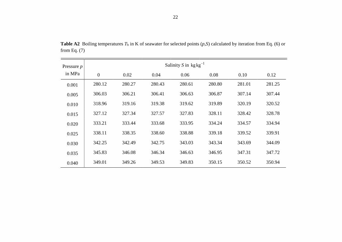
Using Eq. (6) or (7), the boiling temperature bT T= can be calculated by iteration from pressure p and salinity S, or boiling pressure bp p= from temperature T and salinity S, or brine salinity bS S= from p and T. At a given equilibrium state between seawater and water vapor, the properties of the seawater (brine) phase are calculated from Eq. (1) and the properties of the water vapor result from Eq. (8), see Section 4.5.

At brine-vapor equilibrium, vapor is superheated, i.e., at given pressure, the temperature is higher than the saturation temperature of pure water or the pressure at given temperature is below the saturation pressure of pure water.

Note that the Gibbs free energy of liquid water, ( )W ,g p T in Eq. (7), is evaluated from IAPWS-IF97 at conditions where the liquid phase of pure water is metastable. Due to salinity, the boiling temperature elevation can be up to 2 K.

Table A2 shows selected boiling temperatures for given pressures and salinities.

11

4.2 Phase Equilibrium between Seawater and Ice

For the phase equilibrium between seawater and ice Ih, the following condition has to be fulfilled:

( ) ( )IhW , , ,p T S g p Tµ = , (11)

or equivalently:

( ) ( ) ( )W Ihm , , , ,b R T p T S g p T g p Tφ = − , (12)

with ( )W , ,p T Sµ and ( ), ,p T Sφ from Table 1 and ( )W ,g p T from Eq. (4). The molality b is determined from Eq. (3) and the value of the molar gas constant Rm is taken from Table 1 of [2]. The Gibbs free energy of ice Ih ( )Ih ,g p T is calculated from the Gibbs free energy equation of the corresponding IAPWS Release [11]:

( )

( ) ( ) ( ) ( )

Ih W0 0 t

22W

t1

, ( )

Re ln ln 2 ln

τ

ττ τ τ τ=

= −

+ − − + + + − −

∑ k k k k k k kkk

g p T g p s T

T r t t t t t tt

. (13)

The functions ( )0g p and ( )kr p , the triple-point temperature of water WtT , and the reduced

temperature τ are given in [11]. The real constant s0 as well as the complex constants t1, r1, and t2 are listed in Table 2 of [11].

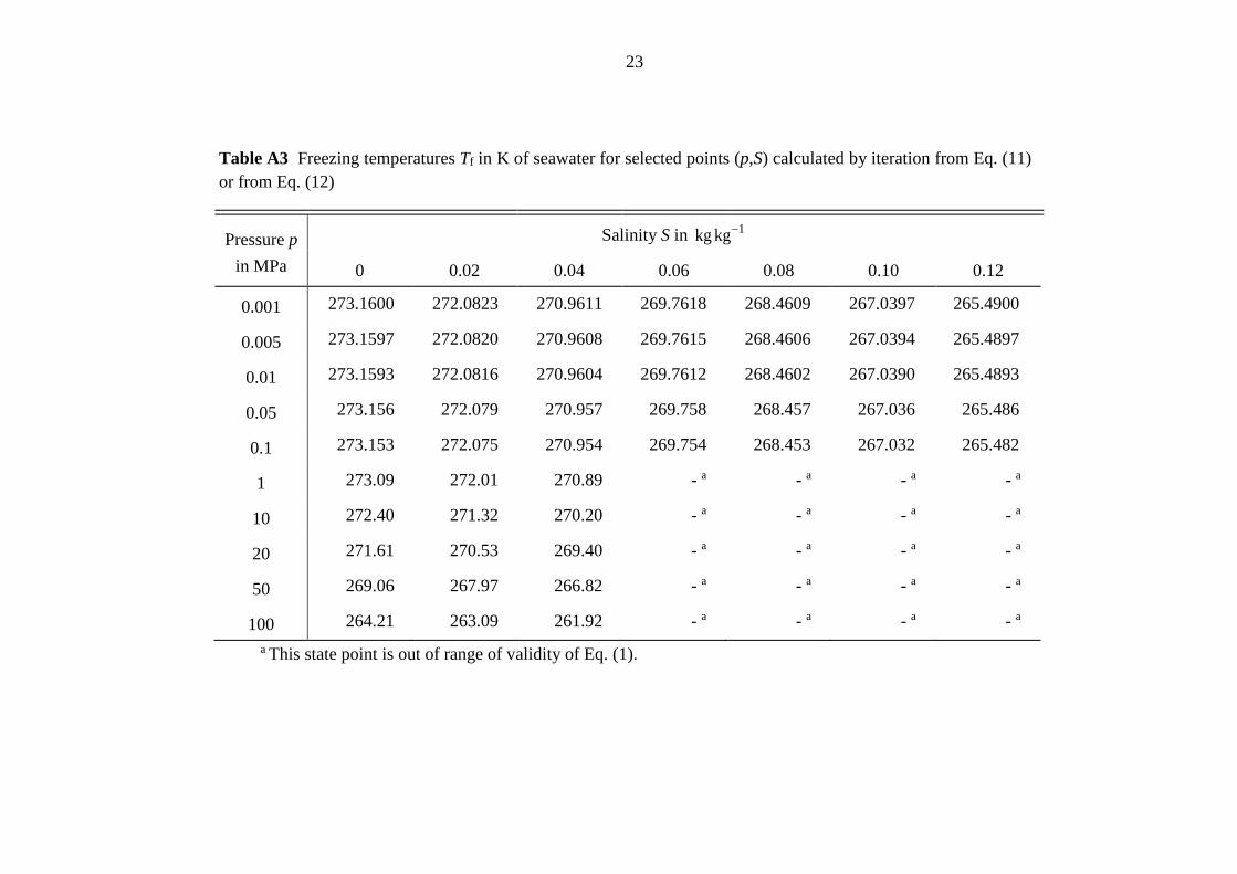
Using Eq. (11) or (12), the freezing temperature fT T= can be calculated by iteration from pressure p and salinity S, or the freezing pressure fp p= from T and S, or brine salinity fS S= from p and T. At a given equilibrium state between seawater and ice, the properties of the seawater (brine) phase are calculated from Eq. (1) and the properties of the ice phase result from Eq. (13), see Section 4.6.

At brine-ice equilibrium, the temperature is lower than the melting temperature at a given pressure of pure ice or the pressure at a given temperature is below the melting pressure of pure ice.

Note that the Gibbs free energy of liquid water ( )W ,g p T in Eq. (12) is evaluated from IAPWS-IF97 at conditions where the liquid phase of pure water is metastable. Due to salinity, the freezing-point depression can be up to 8 K.

Table A3 shows selected freezing temperatures for given pressures and salinities.

4.3 Triple-Point Temperatures and Pressures

The triple-point temperatures tT T= and triple-point pressures tp p= of seawater are calculated for given salinity S by iteration from both Eqs. (6) and (11) or from both Eqs. (7) and (12).

12

Table A4 contains selected triple-point temperatures and triple-point pressures for given salinities.

4.4 Osmotic Pressure

On the two sides of a membrane permeable to water but not to sea salt, equilibrium between liquid water and seawater causes an excess pressure of seawater, the osmotic pressure osmp , computed by iteration from the condition

( ) ( )WW osm , , ,p p T S g p Tµ + = , (14)

or equivalently from

( ) ( ) ( )W Wm osm osm, , , ,b R T p p T S g p p T g p Tφ + = + − , (15)

with Wµ and φ from Table 1 and gW from Eq. (4). The molality b is determined from Eq. (3) and the value of the molar gas constant Rm is taken from Table 1 of [2].

Using Eq. (14) or (15), the osmotic pressure posm is calculated by iteration for pressure p, temperature T, and salinity S.

4.5 Properties of Brine-Vapor Mixture

The properties for the mixture of brine and water vapor, termed brine-vapor mixture, can be computed from the combined Gibbs free energy equation

( ) ( ) ( ) ( )BV vapb, , 1 , , ,g p T S x g p T S x g p T= − + , (16)

where p is the given pressure, T is the given temperature, and S is the given salinity of the seawater mixture including water vapor. The boiling-brine salinity ( )b b ,S S p T= is calculated for pressure p and temperature T using Eq. (6) by iteration. The mass fraction of water vapor in the seawater mixture (vapor fraction) x can be determined from the equation

b1

( , )Sx

S p T= − . (17)

The Gibbs free energy of the brine ( )b, ,g p T S is calculated from Eq. (1) and the Gibbs free energy of water vapor ( )vap ,g p T from Eq. (8).

Brine-vapor properties can be computed from the equation ( )BV , ,g p T S , Eq. (16), and its derivatives in analogy to Table 1.2 The derivatives of the included equation ( )vap ,g p T , Eq. (8),

2 The partial derivatives of BVg with respect to p or T include differentiation of ( )b ,S p T via the

chain rule, making use of Eq. (6). The related terms vanish identically for the first derivatives BV BV( , )p Tg g . This is true, e.g., for the properties v, h, u, and s. But they provide the dominant phase-

change contributions such as latent heat to the second derivatives BV BV BV( , , )pp TT pTg g g [17, 18] which are used, e.g., for the cubic isobaric expansion coefficient αv .

13

for water vapor can be taken from [7]. As an example, the specific enthalpy of brine-vapor mixture is calculated from the equation

( ) ( ) ( ) ( )BV vapb, , 1 , , ,h p T S x h p T S x h p T= − + (18)

where the determination of ( )b, ,h p T S is given in Table 1 and of ( )vap ,h p T in [7].

Further properties such as specific volume ( )BV , ,v p T S , specific internal energy ( )BV , ,u p T S , and specific entropy ( )BV , ,s p T S are computed analogously.

4.6 Properties of Brine-Ice Mixture

The properties for the mixture of brine and ice Ih, termed brine-ice mixture or sea ice, can be computed from the combined Gibbs free energy equation

( ) ( ) ( ) ( )BI Ihf, , 1 , , ,g p T S y g p T S y g p T= − + , (19)

where p is the given pressure, T is the given temperature, and S is the given salinity of the seawater mixture including ice Ih. The freezing-brine salinity ( )f f ,S S p T= is calculated for pressure p and temperature T using Eq. (11) by iteration. The mass fraction of ice Ih in the seawater mixture (ice fraction) y can be determined from the equation

f1

( , )Sy

S p T= − . (20)

The Gibbs free energy of the brine ( )f, ,g p T S is calculated from Eq. (1) and the Gibbs free energy of ice Ih ( )Ih ,g p T from Eq. (13).

Brine-ice mixture properties can be computed from the equation ( )BI , ,g p T S , Eq. (19), and its derivatives in analogy to Table 1.3 The derivatives of the included equation ( )Ih ,g p T , Eq. (13), for ice Ih can be taken from [11]. As an example, the specific enthalpy of brine-ice mixture is calculated from the equation

( ) ( ) ( ) ( )BI Ihf, , 1 , , ,h p T S y h p T S y h p T= − + , (21)

where the determination of ( )f, ,h p T S is given in Table 1 and of ( )Ih ,h p T in [11].

Further properties such as the specific volume ( )BI , ,v p T S , specific internal energy ( )BI , ,u p T S , and specific entropy ( )BI , ,s p T S are computed analogously.

3 The partial derivatives of BIg with respect to p or T include differentiation of ( )f ,S p T via the chain

rule, making use of Eq. (11). The related terms vanish identically for the first derivatives BI BI( , )p Tg g . This is true, e.g., for the properties v, h, u, and s. But they provide the dominant phase-change contributions such as latent heat to the second derivatives BI BI BI( , , )pp TT pTg g g [17, 18] which are used, e.g., for the cubic isobaric expansion coefficient vα .

14

5. Reference States

According to the IAPWS Formulation 2008 for the Thermodynamic Properties of Seawater [2], the specific enthalpy and the specific entropy of seawater calculated from Eq. (1) have been set to zero at 0.101325 MPap = , 273.15 K=T , and 1

n 0.03516504 kg kg−= =S S : 0h = and 0s = ,

where nS is the normal salinity of seawater [10]. The reference state of Eq. (1) for pure liquid water, water vapor, and ice corresponds to the

following values. The specific internal energy and the specific entropy of saturated liquid water at the triple point ( 273.16 KT = , 0.000611657 MPa=p , and 0S = ) are:

0u = and 0s = . From 0u = it follows for the specific enthalpy

10.000611783 kJ kgh −= at this state point. These values correspond to the reference state of IAPWS-IF97.

6. Range of Validity

The equation of state, Eq. (1), is valid for Standard Seawater with sea salt of the Reference Composition [10] in certain regions inside the following pressure, temperature, and salinity ranges

0.3 kPa 100 MPap≤ ≤ , 261 K 353 KT≤ ≤ , and 10 0.12 kg kgS −≤ ≤ . All properties of Table 1 can be calculated with high accuracy in the temperature range

f ( , ) 313 K≤ ≤T p S T for 0.101325 MPa 100 MPa≤ ≤p and 10 0.042 kg kgS −≤ ≤ (Region A in [2])

or for 0.3 kPa 0.101325 MPa≤ ≤p and 10 0.05 kg kgS −≤ ≤ (Region B in [2]).

Outside the above two regions, properties of Table 1 except those depending on pressure derivatives can be calculated with high accuracy near standard atmospheric pressure ( 0.101325 MPap = ).

for f ( , ) 353 K≤ ≤T p S T and 10 0.12 kg kgS −≤ ≤ (Region C in [2]). Density is very well extrapolated by this formulation up to the highest salinity values at low

temperatures. In the range of higher salinity and higher temperature near standard atmospheric pressure, density is described with lower accuracy and quantities computed from its extrapolated derivatives may even be invalid. Due to the lack of experimental data, no statements could be made in the release on the IAPWS formulation 2008 [2] about the accuracy at high pressures for temperatures greater than 313 K and salinities greater than 0.042.

Restrictions regarding certain properties outside these ranges are described in detail in Section 6 of the IAPWS Release [2]. Reference [2] also contains a graphical representation of the range of validity in a p-T-S plot.

15

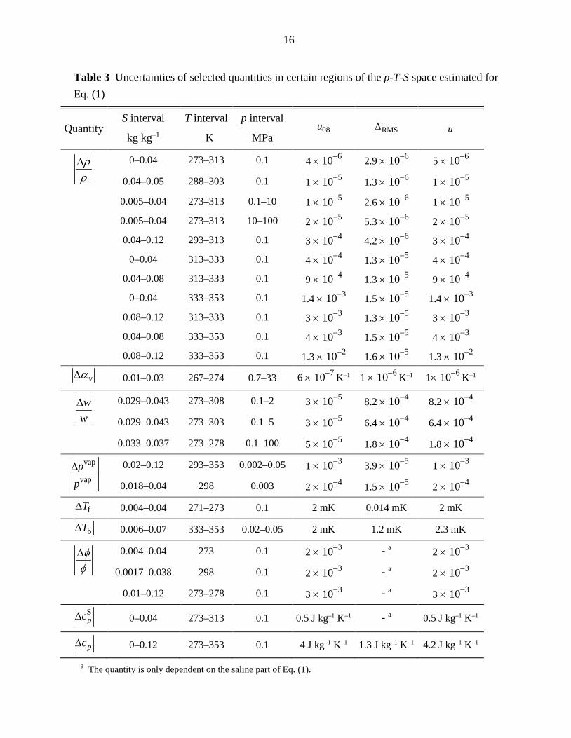
7. Uncertainty

A summary of estimated combined standard uncertainties u (coverage factor =1k ) of selected quantities using IAPWS-95 for the water part in certain regions of the p-T-S space is given in Table 7 in the IAPWS release on the IAPWS formulation 2008 [2]. By using IAPWS-IF97 instead of IAPWS-95, some deviations caused by the difference between IAPWS-IF97 and IAPWS-95 must be added to the uncertainties. The total uncertainty using IAPWS-IF97 can be estimated by the equation

= + ∆2 208 RMSu u , (22)

where u08 represents the uncertainty of the 2008 IAPWS seawater formulation [2] (which uses IAPWS-95 for pure-water properties), and ∆RMS represents the root-mean-square of the deviations caused by the difference between IAPWS-IF97 and IAPWS-95 and is computed from

2RMS

1

1 ( )N

nn

xN =

∆ = ∆∑ , where ∆xn can be either absolute or percentage difference between the

corresponding quantities x ; N is the number of ∆xn values (100 000 points uniformly distributed over the respective range of validity were used to calculate Table 3).

A summary of estimated values u08, ∆RMS , and u is given in Table 3.

8. Computing Time for the IAPWS Seawater Functions

One important reason to use IAPWS-IF97 instead of IAPWS-95 for calculating the water part of the IAPWS seawater functions is the computing-speed difference between these two standards. The relations of the computing speed of the seawater functions of the 2008 IAPWS seawater formulation [2] (which uses IAPWS-95) in comparison with the industrial formulation for seawater given herein (using IAPWS-IF97) were investigated and reported in [1], where improvements in speed by factors on the order of 100 or 200 were reported. While the observed improvement will depend on the efficiency with which IAPWS-95 is programmed (and also on details of the machine and compiler used), the use of IAPWS-IF97 clearly produces a significant reduction in computing time.

16

Table 3 Uncertainties of selected quantities in certain regions of the p-T-S space estimated for Eq. (1)

Quantity S interval

kg kg–1

T interval

K

p interval

MPa 08u ∆RMS u

ρρ∆

0–0.04 273–313 0.1 4 × 10−6 2.9 × 10−6 5 × 10−6

0.04–0.05 288–303 0.1 1 × 10−5 1.3 × 10−6 1 × 10−5

0.005–0.04 273–313 0.1–10 1 × 10−5 2.6 × 10−6 1 × 10−5 0.005–0.04 273–313 10–100 2 × 10−5 5.3 × 10−6 2 × 10−5 0.04–0.12 293–313 0.1 3 × 10−4 4.2 × 10−6 3 × 10−4 0–0.04 313–333 0.1 4 × 10−4 1.3 × 10−5 4 × 10−4 0.04–0.08 313–333 0.1 9 × 10−4 1.3 × 10−5 9 × 10−4 0–0.04 333–353 0.1 1.4 × 10−3 1.5 × 10−5 1.4 × 10−3 0.08–0.12 313–333 0.1 3 × 10−3 1.3 × 10−5 3 × 10−3 0.04–0.08 333–353 0.1 4 × 10−3 1.5 × 10−5 4 × 10−3 0.08–0.12 333–353 0.1 1.3 × 10−2 1.6 × 10−5 1.3 × 10−2

vα∆ 0.01–0.03 267–274 0.7–33 6 × 10−7 K–1 1 × 10−6 K–1 1× 10−6 K–1

ww∆

0.029–0.043 273–308 0.1–2 3 × 10−5 8.2 × 10−4 8.2 × 10−4

0.029–0.043 273–303 0.1–5 3 × 10−5 6.4 × 10−4 6.4 × 10−4

0.033–0.037 273–278 0.1–100 5 × 10−5 1.8 × 10−4 1.8 × 10−4 vap

vap p

p∆

0.02–0.12 293–353 0.002–0.05 1 × 10−3 3.9 × 10−5 1 × 10−3

0.018–0.04 298 0.003 2 × 10−4 1.5 × 10−5 2 × 10−4

fT∆ 0.004–0.04 271–273 0.1 2 mK 0.014 mK 2 mK

bT∆ 0.006–0.07 333–353 0.02–0.05 2 mK 1.2 mK 2.3 mK

φφ∆

0.004–0.04 273 0.1 2 × 10−3 - a 2 × 10−3

0.0017–0.038 298 0.1 2 × 10−3 - a 2 × 10−3

0.01–0.12 273–278 0.1 3 × 10−3 - a 3 × 10−3 Spc∆

0–0.04 273–313 0.1 0.5 J kg–1 K–1 - a 0.5 J kg–1 K–1

pc∆ 0–0.12 273–353 0.1 4 J kg–1 K–1 1.3 J kg–1 K–1 4.2 J kg–1 K–1

a The quantity is only dependent on the saline part of Eq. (1).

17

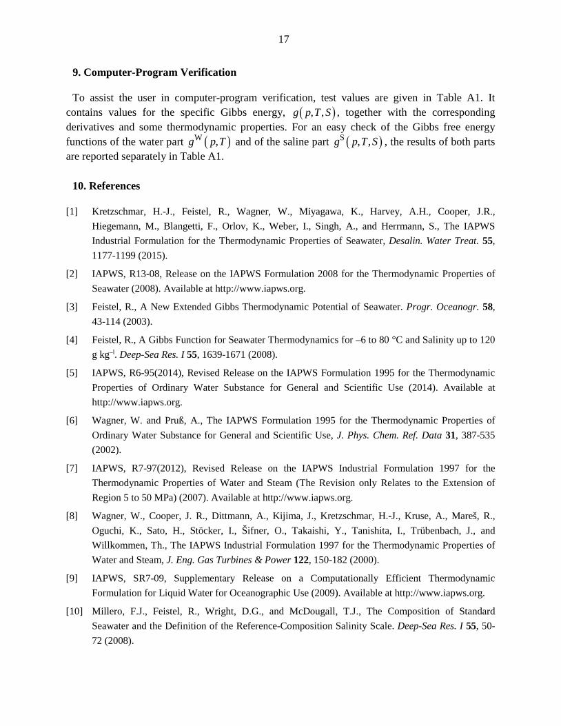
9. Computer-Program Verification

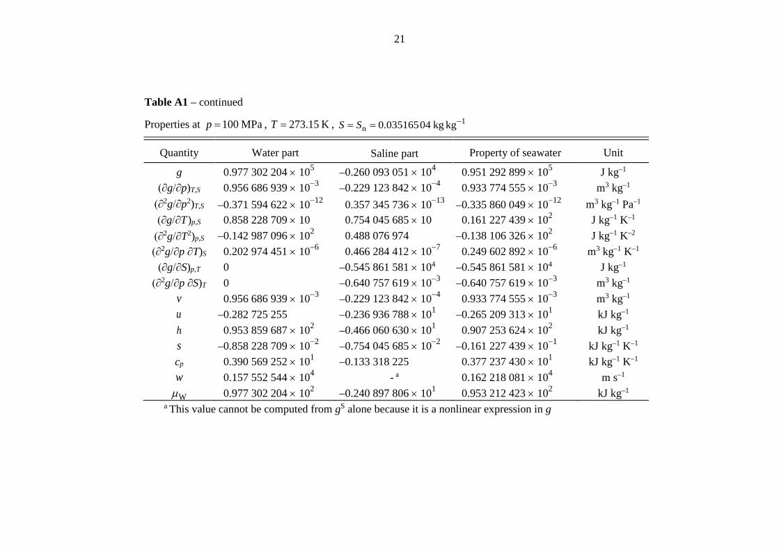
To assist the user in computer-program verification, test values are given in Table A1. It contains values for the specific Gibbs energy, ( ), ,g p T S , together with the corresponding derivatives and some thermodynamic properties. For an easy check of the Gibbs free energy functions of the water part ( )W ,g p T and of the saline part ( )S , ,g p T S , the results of both parts are reported separately in Table A1.

10. References

[1] Kretzschmar, H.-J., Feistel, R., Wagner, W., Miyagawa, K., Harvey, A.H., Cooper, J.R., Hiegemann, M., Blangetti, F., Orlov, K., Weber, I., Singh, A., and Herrmann, S., The IAPWS Industrial Formulation for the Thermodynamic Properties of Seawater, Desalin. Water Treat. 55, 1177-1199 (2015).

[2] IAPWS, R13-08, Release on the IAPWS Formulation 2008 for the Thermodynamic Properties of Seawater (2008). Available at http://www.iapws.org.

[3] Feistel, R., A New Extended Gibbs Thermodynamic Potential of Seawater. Progr. Oceanogr. 58, 43-114 (2003).

[4] Feistel, R., A Gibbs Function for Seawater Thermodynamics for –6 to 80 °C and Salinity up to 120 g kg–l. Deep-Sea Res. I 55, 1639-1671 (2008).

[5] IAPWS, R6-95(2014), Revised Release on the IAPWS Formulation 1995 for the Thermodynamic Properties of Ordinary Water Substance for General and Scientific Use (2014). Available at http://www.iapws.org.

[6] Wagner, W. and Pruß, A., The IAPWS Formulation 1995 for the Thermodynamic Properties of Ordinary Water Substance for General and Scientific Use, J. Phys. Chem. Ref. Data 31, 387-535 (2002).

[7] IAPWS, R7-97(2012), Revised Release on the IAPWS Industrial Formulation 1997 for the Thermodynamic Properties of Water and Steam (The Revision only Relates to the Extension of Region 5 to 50 MPa) (2007). Available at http://www.iapws.org.

[8] Wagner, W., Cooper, J. R., Dittmann, A., Kijima, J., Kretzschmar, H.-J., Kruse, A., Mareš, R., Oguchi, K., Sato, H., Stöcker, I., Šifner, O., Takaishi, Y., Tanishita, I., Trübenbach, J., and Willkommen, Th., The IAPWS Industrial Formulation 1997 for the Thermodynamic Properties of Water and Steam, J. Eng. Gas Turbines & Power 122, 150-182 (2000).

[9] IAPWS, SR7-09, Supplementary Release on a Computationally Efficient Thermodynamic Formulation for Liquid Water for Oceanographic Use (2009). Available at http://www.iapws.org.

[10] Millero, F.J., Feistel, R., Wright, D.G., and McDougall, T.J., The Composition of Standard Seawater and the Definition of the Reference-Composition Salinity Scale. Deep-Sea Res. I 55, 50-72 (2008).

18

[11] IAPWS, R10-06, Revised Release on the Equation of State 2006 for H2O Ice Ih (2009). Available at http://www.iapws.org.

[12] Feistel, R. and Wagner, W., A New Equation of Sate for H2O Ice Ih. J. Phys. Chem. Ref. Data 35, 1021-1047 (2006).

[13] IOC, SCOR, IAPSO, The International Thermodynamic Equation of Seawater - 2010: Calculation and Use of Thermodynamic Properties. Intergovernmental Oceanographic Commission, Manuals and Guides No. 56, UNESCO, Paris (2010). Available at http://www.TEOS-10.org.

[14] IAPWS, AN3-07(2014), Revised Advisory Note No. 3: Thermodynamic Derivatives from IAPWS Formulations (2014). Available at http://www.iapws.org.

[15] IAPWS, R14-08(2011), Revised Release on the Pressure along the Melting and Sublimation Curves of Ordinary Water Substance (2011). Available at http://www.iapws.org.

[16] Wagner, W., Riethmann, T., Feistel, R., and Harvey, A.H., New Equations for the Sublimation Pressure and Melting Pressure of H2O Ice Ih. J. Phys. Chem. Ref. Data 40, 043103 (2011).

[17] Feistel, R., Wright, D.G., Kretzschmar, H.-J., Hagen, E., Herrmann, S., and Span, R., Thermodynamic Properties of Sea Air. Ocean Sci. 6, 91-141 (2010).

[18] Feistel, R., Wright, D.G., Jackett, D.R., Miyagawa, K., Reissmann, J.H., Wagner, W., Overhoff, U., Guder, C., Feistel, A., and Marion, G.M., Numerical Implementation and Oceanographic Application of the Thermodynamic Potentials of Liquid Water, Water Vapour, Ice, Seawater and Humid Air – Part 1: Background and Equations. Ocean Sci. 6, 633-677 (2010).

19

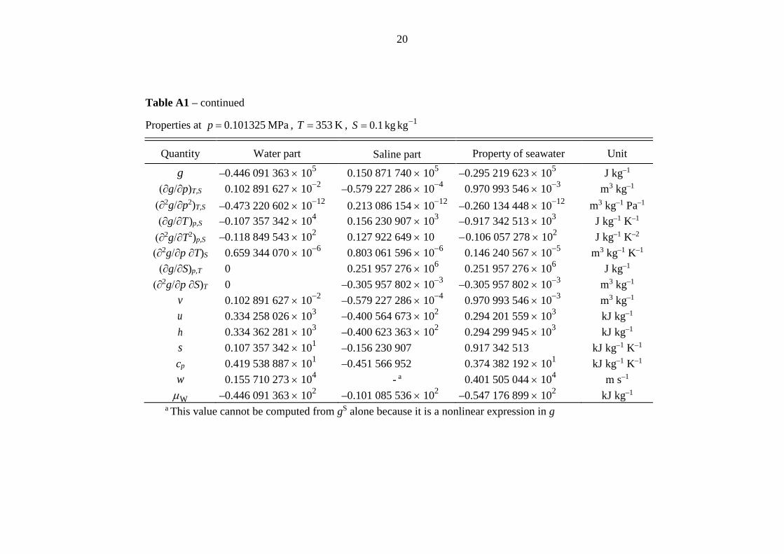
APPENDIX

Table A1 Numerical check values for the water part computed from ( )W ,g p T , Eq. (4), and its derivatives, for the saline part computed from ( )S , ,g p T S , Eq. (5), and its derivatives, for the seawater properties computed from the Gibbs function ( ), ,g p T S , Eq. (1) and its derivatives and for selected seawater properties of Table 1 at given points ( ), ,p T S

Properties at 0.101325 MPa=p , 273.15 K=T , 1n 0.03516504 kg kgS S −= =

Quantity Water part Saline part Property of seawater Unit

g 0.101 359 446 × 103 –0.101 342 742 × 103 0.167 04 × 10−1 J kg–1 (∂g/∂p)T,S 0.100 015 572 × 10−2 –0.274 957 224 × 10−4 0.972 659 995 × 10−3 m3 kg–1 (∂2g/∂p2)T,S –0.508 885 499 × 10−12 0.581 535 172 × 10−13 –0.450 731 982 × 10−12 m3 kg–1 Pa–1 (∂g/∂T)p,S 0.147 711 823 –0.147 643 376 0.684 47 × 10−4 J kg–1 K–1 (∂2g/∂T2)p,S –0.154 473 013 × 102 0.852 861 151 –0.145 944 401 × 102 J kg–1 K–2 (∂2g/∂p ∂T)S –0.676 992 620 × 10−7 0.119 286 787 × 10−6 0.515 875 254 × 10−7 m3 kg–1 K–1 (∂g/∂S)p,T 0 0.639 974 067 × 105 0.639 974 067 × 105 J kg–1 (∂2g/∂p ∂S)T 0 –0.759 615 412 × 10−3 –0.759 615 412 × 10−3 m3 kg–1

v 0.100 015 572 × 10−2 –0.274 957 224 × 10−4 0.972 659 995 × 10−3 m3 kg–1 u –0.403 288 161 × 10−1 –0.582 279 494 × 10−1 –0.985 567 655 × 10−1 kJ kg–1 h 0.610 119 617 × 10−1 –0.610 139 535 × 10−1 –0.199 18 × 10−5 kJ kg–1 s –0.147 711 823 × 10−3 0.147 643 376 × 10−3 –0.684 47 × 10−7 kJ kg–1 K–1 cp 0.421 943 034 × 101 –0.232 959 023 0.398 647 132 × 101 kJ kg–1 K–1 w 0.140 243 979 × 104 - a 0.144 907 123 × 104 m s–1

Wµ 0.101 359 446 –0.235 181 411 × 101 –0.225 045 466 × 101 kJ kg–1 a This value cannot be computed from gS alone because it is a nonlinear expression in g

20

Table A1 – continued

Properties at 0.101325 MPa=p , 353 K=T , 10.1 kg kgS −=

Quantity Water part Saline part Property of seawater Unit

g –0.446 091 363 × 105 0.150 871 740 × 105 –0.295 219 623 × 105 J kg–1 (∂g/∂p)T,S 0.102 891 627 × 10−2 –0.579 227 286 × 10−4 0.970 993 546 × 10−3 m3 kg–1 (∂2g/∂p2)T,S –0.473 220 602 × 10−12 0.213 086 154 × 10−12 –0.260 134 448 × 10−12 m3 kg–1 Pa–1 (∂g/∂T)p,S –0.107 357 342 × 104 0.156 230 907 × 103 –0.917 342 513 × 103 J kg–1 K–1 (∂2g/∂T2)p,S –0.118 849 543 × 102 0.127 922 649 × 10 – 0.106 057 278 × 102 J kg–1 K–2 (∂2g/∂p ∂T)S 0.659 344 070 × 10−6 0.803 061 596 × 10−6 0.146 240 567 × 10−5 m3 kg–1 K–1 (∂g/∂S)p,T 0 0.251 957 276 × 106 0.251 957 276 × 106 J kg–1 (∂2g/∂p ∂S)T 0 –0.305 957 802 × 10−3 –0.305 957 802 × 10−3 m3 kg–1

v 0.102 891 627 × 10−2 –0.579 227 286 × 10−4 0.970 993 546 × 10−3 m3 kg–1 u 0.334 258 026 × 103 –0.400 564 673 × 102 0.294 201 559 × 103 kJ kg–1 h 0.334 362 281 × 103 –0.400 623 363 × 102 0.294 299 945 × 103 kJ kg–1 s 0.107 357 342 × 101 –0.156 230 907 0.917 342 513 kJ kg–1 K–1 cp 0.419 538 887 × 101 –0.451 566 952 0.374 382 192 × 101 kJ kg–1 K–1 w 0.155 710 273 × 104 - a 0.401 505 044 × 104 m s–1

Wµ –0.446 091 363 × 102 –0.101 085 536 × 102 –0.547 176 899 × 102 kJ kg–1 a This value cannot be computed from gS alone because it is a nonlinear expression in g

21

Table A1 – continued

Properties at 100 MPa=p , 273.15 K=T , 1n 0.03516504 kg kg−= =S S

Quantity Water part Saline part Property of seawater Unit

g 0.977 302 204 × 105 –0.260 093 051 × 104 0.951 292 899 × 105 J kg–1 (∂g/∂p)T,S 0.956 686 939 × 10−3 –0.229 123 842 × 10−4 0.933 774 555 × 10−3 m3 kg–1 (∂2g/∂p2)T,S –0.371 594 622 × 10−12 0.357 345 736 × 10−13 –0.335 860 049 × 10−12 m3 kg–1 Pa–1 (∂g/∂T)p,S 0.858 228 709 × 10 0.754 045 685 × 10 0.161 227 439 × 102 J kg–1 K–1 (∂2g/∂T2)p,S –0.142 987 096 × 102 0.488 076 974 –0.138 106 326 × 102 J kg–1 K–2 (∂2g/∂p ∂T)S 0.202 974 451 × 10−6 0.466 284 412 × 10−7 0.249 602 892 × 10−6 m3 kg–1 K–1 (∂g/∂S)p,T 0 –0.545 861 581 × 104 –0.545 861 581 × 104 J kg–1 (∂2g/∂p ∂S)T 0 –0.640 757 619 × 10−3 –0.640 757 619 × 10−3 m3 kg–1

v 0.956 686 939 × 10−3 –0.229 123 842 × 10−4 0.933 774 555 × 10−3 m3 kg–1 u –0.282 725 255 –0.236 936 788 × 101 –0.265 209 313 × 101 kJ kg–1 h 0.953 859 687 × 102 –0.466 060 630 × 101 0.907 253 624 × 102 kJ kg–1 s –0.858 228 709 × 10−2 –0.754 045 685 × 10−2 –0.161 227 439 × 10−1 kJ kg–1 K–1 cp 0.390 569 252 × 101 –0.133 318 225 0.377 237 430 × 101 kJ kg–1 K–1 w 0.157 552 544 × 104 - a 0.162 218 081 × 104 m s–1

Wµ 0.977 302 204 × 102 –0.240 897 806 × 101 0.953 212 423 × 102 kJ kg–1 a This value cannot be computed from gS alone because it is a nonlinear expression in g

22

Table A2 Boiling temperatures Tb in K of seawater for selected points (p,S) calculated by iteration from Eq. (6) or from Eq. (7)

Pressure p

in MPa

Salinity S in 1kg kg−

0 0.02 0.04 0.06 0.08 0.10 0.12

0.001 280.12 280.27 280.43 280.61 280.80 281.01 281.25

0.005 306.03 306.21 306.41 306.63 306.87 307.14 307.44

0.010 318.96 319.16 319.38 319.62 319.89 320.19 320.52

0.015 327.12 327.34 327.57 327.83 328.11 328.42 328.78

0.020 333.21 333.44 333.68 333.95 334.24 334.57 334.94

0.025 338.11 338.35 338.60 338.88 339.18 339.52 339.91

0.030 342.25 342.49 342.75 343.03 343.34 343.69 344.09

0.035 345.83 346.08 346.34 346.63 346.95 347.31 347.72

0.040 349.01 349.26 349.53 349.83 350.15 350.52 350.94

23

Table A3 Freezing temperatures Tf in K of seawater for selected points (p,S) calculated by iteration from Eq. (11) or from Eq. (12)

Pressure p

in MPa

Salinity S in 1kg kg−

0 0.02 0.04 0.06 0.08 0.10 0.12

0.001 273.1600 272.0823 270.9611 269.7618 268.4609 267.0397 265.4900

0.005 273.1597 272.0820 270.9608 269.7615 268.4606 267.0394 265.4897

0.01 273.1593 272.0816 270.9604 269.7612 268.4602 267.0390 265.4893

0.05 273.156 272.079 270.957 269.758 268.457 267.036 265.486

0.1 273.153 272.075 270.954 269.754 268.453 267.032 265.482

1 273.09 272.01 270.89 - a - a - a - a

10 272.40 271.32 270.20 - a - a - a - a

20 271.61 270.53 269.40 - a - a - a - a

50 269.06 267.97 266.82 - a - a - a - a

100 264.21 263.09 261.92 - a - a - a - a a This state point is out of range of validity of Eq. (1).

24

Table A4 Triple-point temperatures Tt and related triple-point pressures pt of seawater for selected salinities S calculated by iteration from both Eqs. (6) and (11) or from both Eqs. (7) and (12)

Salinity S in 1kg kg− 0 0.02 0.04 0.06 0.08 0.10 0.12

Triple-point temperature Tt in K 273.16 272.08 270.96 269.76 268.46 267.04 265.49

Triple-point pressure pt in kPa 0.61168 0.55953 0.50961 0.46073 0.41257 0.36524 0.31932