adverse selection in the annuity market and the role for

Adverse Selection in the Annuity Market and the Role for Social SecurityAuthor(s): Roozbeh HosseiniSource: Journal of Political Economy, Vol. 123, No. 4 (August 2015), pp. 941-984Published by: The University of Chicago PressStable URL: http://www.jstor.org/stable/10.1086/681593 .

Accessed: 30/08/2015 16:09

Your use of the JSTOR archive indicates your acceptance of the Terms & Conditions of Use, available at .http://www.jstor.org/page/info/about/policies/terms.jsp

.JSTOR is a not-for-profit service that helps scholars, researchers, and students discover, use, and build upon a wide range ofcontent in a trusted digital archive. We use information technology and tools to increase productivity and facilitate new formsof scholarship. For more information about JSTOR, please contact [email protected].

.

The University of Chicago Press is collaborating with JSTOR to digitize, preserve and extend access to Journalof Political Economy.

http://www.jstor.org

This content downloaded from 129.219.247.33 on Sun, 30 Aug 2015 16:09:01 PMAll use subject to JSTOR Terms and Conditions

http://www.jstor.org/action/showPublisher?publisherCode=ucpress

http://www.jstor.org/stable/10.1086/681593?origin=JSTOR-pdf

http://www.jstor.org/page/info/about/policies/terms.jsp


Adverse Selection in the Annuity Market
and the Role for Social Security
Roozbeh Hosseini

Arizona State University

I study the role of social security in providing insurance when thereis adverse selection in the annuity market. I calculate welfare gain

I. I

I amprojeFinkeChrisGustanars,mousrema

1 EFinkeother

Electro[ Journa© 2015

from mandatory annuitization in the social security system relativeto a laissez-faire benchmark, using a model in which individuals haveprivate information about their mortality. I estimate large heteroge-neity in mortality using the Health and Retirement Study. Despite that,I find small welfare gain from mandatory annuitization. Social securityhas a large effect on annuity prices because it crowds out demand byhigh-mortality individuals. Welfare gain would have been significantlylarger in the absence of this effect.

ntroduction

Mandatory annuitization is a key feature of the current US social securitysystem. The value of this feature is derived from its ability to overcomepotential inefficiencies due to adverse selection in the annuity market.1

grateful to Larry Jones and V. V. Chari for their gracious guidance throughout thisct. I also thank Laurence Ales, Marco Bassetto, Neil Doherty, Mike Golosov, Amylstein, Narayana Kocherlakota, Pricila Maziero, Ellen McGrattan, Olivia Mitchell,Phelan, Jim Poterba, Jose-Vıctor Rıos-Rull, Richard Rogerson, Todd Schoellman,vo Ventura, Pierre Yared, Steve Zeldes, and participants at several workshops, semi-and conferences for helpful comments and discussion. The editor and two anony-referees providedmany helpful suggestions that substantially improved the paper. Allining errors are mine. Data are provided as supplementary material online.xistence of adverse selection is well documented by Friedman and Warshawsky ð1990Þ,lstein and Poterba ð2002, 2004, 2006Þ, and McCarthy and Mitchell ð2003Þ, amongs.

nically published June 30, 2015l of Political Economy, 2015, vol. 123, no. 4]by The University of Chicago. All rights reserved. 0022-3808/2015/12304-0007$10.00

941



The purpose of this paper is to quantify the value of mandatory annu-itization in the current US social security system using a framework in

942 journal of political economy

which informational frictions in the annuity market are explicitly mod-eled.To this end, I develop a dynamic life cycle model in which individuals

have private information about their mortality. Uncertainty about thetime of death generates demand for longevity insurance. In this environ-ment individuals can purchase annuity contracts at linear prices. Con-tracts are nonexclusive, and insurers cannot observe individuals’ trades.The lack of observability in my model implies that insurers cannot clas-sify individuals by their risk types. As a result, the unit price of insur-ance coverage is identical for all agents. Individuals with higher mor-tality ðwho, on average, die earlierÞ demand little insurance ðor nothingat allÞ. This makes lower mortality types ðtypes with higher risks of sur-vivalÞ more represented in the market. This, in turn, leads the equilib-rium price of annuities to be higher than the overall actuarially fair valueof their payment.In this environment, I define and characterize a set of ex ante efficient

ðfirst-bestÞ allocations. I show that these allocations are independent ofindividuals’ mortality risk type and contingent only on survival, which ispublicly observed. This feature implies that ex ante efficient allocationscan be implemented by a system of mandatory annuitization in whichevery individual is taxed, lump-sum, before retirement and receives abenefit contingent on survival after retirement. The ex ante efficientallocation will be the benchmark for the best outcome that any socialsecurity system can achieve.The environment I study has three important features. First, individ-

uals know all relevant information about their mortality risk types at thebeginning of life. This assumes away any possibility of insuring againstthe realization of risk type in the market and biases the results in favor ofmandatory annuitization. Second, there is no heterogeneity other thanmortality types. This implies that optimal policies are uniform acrossindividuals. Finally, there are no distortionary effects of policy on laborsupply and retirement decisions. Therefore, the focus will be only on in-efficiencies caused by adverse selection and the beneficial role of man-datory annuitization.A key object in the model is the distribution of mortality risk types.

This distribution determines the extent of private information in theeconomy. Following the demography literature, heterogeneity in mor-tality risk is modeled as a frailty parameter that shifts the force of mor-tality ðsee, e.g., Vaupel, Manton, and Stallard 1979; Manton, Stallard, andVaupel 1981; Butt and Haberman 2004Þ. This parameter, once realized atbirth, stays constant throughout one’s lifetime. Individuals with a higher



frailty parameter are more likely to die at any given age. I parameterizethe initial distribution of mortality types and use data on subjective sur-

adverse selection in the annuity market 943

vival probabilities in the Health and Retirement Study ðHRSÞ to estimatethose parameters.2

The model is calibrated to match two key features in the data: ð1Þ theaverage replacement ratio in the current US social security system ðthisdetermines the extent of annuitization through social securityÞ andð2Þ the average fraction of retirement wealth that is annuitized outsidesocial security ðthis determines the demand for annuities in the currentUS systemÞ.The quantitative exercise of this paper consists of welfare compari-

sons between three economies: ð1Þ an economy with no social securityin which individuals share their longevity risks only through an annuitymarket, ð2Þ the same economy with the addition of a social securitysystem calibrated to the current US system, and ð3Þ an economy in whichex ante efficient allocations are implemented. To highlight the impor-tance of market response to policy, I report all welfare calculations underthree assumptions: no annuity market, annuity markets with full infor-mation, and annuity markets with private information.The three main findings of the paper are as follows: ð1Þ The overall

welfare gain from having mandatory annuitization through the currentUS social security system relative to a benchmark without social securityis 0.07 percent of consumption. ð2Þ Social security has a large effect onthe annuity price. This effect comes as a result of crowding out of de-mand for annuities by low-survival individuals. This price effect has anegative welfare impact of 0.35 percent of consumption. In other words,in the absence of this price effect, the welfare gain from social securitywould have been as large as 0.42 percent. ð3Þ In the absence of an an-nuity market, the welfare gain from annuitization through the currentUS social security system is 2.68 percent of consumption. This is a sig-nificant welfare gain and indicates the extent of uninsured survival riskin the absence of any insurance mechanism.The upshot of these findings is that assessing how useful social security

is in providing annuity insurance depends on assumptions about im-perfect annuity insurance markets. If an annuity market is missing forexogenous reasons, then mandatory annuitization through social secu-rity can have large welfare gains. If annuity markets exist but are im-perfect because of adverse selection, then mandatory annuitization can

2 Hurd and McGarry ð1995, 2002Þ and Smith, Taylor, and Sloan ð2001Þ document thatthese probabilities are consistent with life tables and ex post mortality experience. Theyargue that they are good predictors of individuals’ mortality.



be welfare improving. But they may also drive good risk types out of theannuity market and exacerbate adverse selection. This crowding-out


effect can significantly reduce welfare gains from the policy. This is inline with findings by Golosov and Tsyvinski ð2007Þ and Krueger and Perrið2011Þ, who study endogenous insurance markets and responses to pub-lic provision of insurance.Related literature.—The role of mandatory annuitization in the annuity

market with adverse selection was first studied by Eckstein, Eichenbaum,and Peled ð1985Þ and Eichenbaum and Peled ð1987Þ. The contributionof this paper is the quantitative assessment of the welfare gains due tomandatory annuitization in the current US system.There is a broad literature on measuring the insurance value of an-

nuitization for representative life cycle consumers ðe.g., Kotlikoff andSpivak 1981; Mitchell et al. 1999; Brown 2001; Davidoff, Brown, and Dia-mond 2005Þ. The exercise in this literature is to determine how muchincremental, nonannuitized wealth would be equivalent to providing ac-cess to actuarially fair annuity markets.3 A key feature of all these stud-ies is the static comparison between full insurance and no insurance. Incontrast, in the current paper I allow for annuitization through privateannuity markets at retirement. This allows me to distinguish betweenrisk sharing that is provided by the market and self-insurance and tostudy how risk sharing changes in response to changes in publicly pro-vided insurance.Einav, Finkelstein, and Shrimpf ð2010Þ study the welfare cost of private

information in the United Kingdom’s mandatory annuity market. Theyreport welfare gains from imposing further mandates that can imple-ment the first-best. In contrast, in this paper the comparison is madebetween an economy with mandatory annuitization from social securityand a laissez-faire economy. In both economies, participation in an an-nuity market is voluntary. However, outcome in a laissez-faire economyis inefficient because of adverse selection. The goal is to evaluate howsuccessful the current social security system is in improving outcomesover laissez-faire.The rest of the paper is structured as follows: Section II describes the

environment, defines and characterizes efficient allocations, and definesthe equilibrium. Section III describes the parametric specifications ofthe mortality model. Section IV describes the data and the calibrationprocedure. Section V reports results of welfare comparisons. Section VIexplores sensitivity and robustness. Finally, Section VII presents con-clusions.

3 The study by Lockwood ð2012Þ is an exception in that he considers the comparison
between no annuity and an annuity available at actuarially unfair market rates.


II. Model


A. Environment

The economy starts at date 0 and ends at T ð1 ≤ T < `Þ. Individuals areborn at the beginning of period 0 and face an uncertain life span. Anindividual who survives to age t faces the uncertainty of surviving to aget1 1 or dying at the end of age t. Anyone who survives to age T will die atthe end of that age. There is a set of individual frailty types, V5 ½v;�v� ⊆ R1.Frailty type v ∈ V determines the probability of survival to each age t. In-dividuals with lower v have a higher probability of survival ðand longer ex-pected lifetimesÞ. Individual type, v, is private information.Suppose there is a well-defined distribution G 0 ∈ DðVÞ with full sup-

port. Let PtðvÞ be the probability of survival to age t at age 0. Therefore,the joint probability that an individual’s type is in the set Z ⊆ V and sur-vives to age t is mtðZ Þ5 ∫v∈ZPtðvÞdG 0ðvÞ.Individuals who die exit the economy. Therefore, in each age the dis-

tribution of types ðconditional on survivalÞ becomesmore skewed towardthe higher survival types ði.e., lower v typesÞ. Let Gt be the distribution oftypes conditional on survival to age t; then the fraction of people withtype in any set Z ⊆ V is

GtðZ Þ5Ez∈Z

PtðzÞdG 0ðzÞ

Ev∈V

PtðvÞdG 0ðvÞ∀Z ⊆ V: ð1Þ

Individuals have time-separable utility over consumption, uð�Þ, as longas they live. They also enjoy utility from leaving a bequest at the time ofdeath, vð�Þ. These functions are assumed to be twice continuously differ-entiable with u 0, v 0 > 0 and u 0 0, v 0 0 < 0 and satisfy the usual Inada condi-tions. Let xtðvÞ5 Pt11ðvÞ=PtðvÞ be the one-period survival rate for type v

ðprobability of surviving to age t 1 1 conditioned on being alive at tÞ.Then type v’s utility out of a given sequence of consumption, ct, and be-quest, bt, is

oT

t50

PtðvÞbtfuðctÞ1 ½12 xt11ðvÞ�bvðbtÞg; 0 < b ≤ 1:

Each individual is endowed with a unit of labor endowment that isinelastically supplied for age-dependent wage wt in every period t ≤ J < T.All individuals work until age J and then retire. There is also a savingtechnology with gross rate R ≥ 1=b.



An allocation is a map from agents’ type to a positive real line, that is,


ct : V→ R1; 0 ≤ t ≤ T ;

bt : V→ R1; 0 ≤ t ≤ T :

Here, ctðvÞ is the consumption of all v type individuals conditioned ontheir survival at age t ðand, similarly, btðvÞ is the bequest that type v leavesif he dies at the end of age tÞ.An allocation is feasible if

EoTt50

PtðvÞRt

�ctðvÞ1 12 xt11ðvÞ

RbtðvÞ

�dG 0ðvÞ

5 EoJt50

PtðvÞRt

wtdG 0ðvÞ:ð2Þ

Individuals face two types of risks here. From the ex ante point of viewðbefore birthÞ, they face the risk of their type realization. Individuals whosetype v implies a higher survival probability need more resources to fi-nance consumption through their lifetimes relative to those types whohave lower survival. Also, upon realization of frailty types v, individualsface the risk of outliving their assets.

B. Ex Ante Efficient Allocation

A benchmark for perfect risk sharing against both realization of typesand time of death is the ex ante efficient ðor first-bestÞ allocation. That isthe solution to the problem of a social planner who maximizes the ex-pected discounted utility of individuals behind the veil of ignorance, thatis, before agents are born:

maxct ðvÞ;bt ðvÞ ≥ 0

EoTt50

PtðvÞbtfuðctðvÞÞ1 ½12 xt11ðvÞ�bvðbtðvÞÞgdgG 0ðvÞ

subject to ð2Þ.It is straightforward to verify that the allocations that solve the prob-

lem above must satisfy

ctðvÞ5 ctðv 0Þ5 ct for all v; v 0 ∈ V; ∀t ;btðvÞ5 btðv 0Þ5 bt for all v; v0 ∈ V; ∀t ;

and

u 0ðctÞ5 bRu 0ðct11Þ5 bRv 0ðbtÞ:As is evident from the above equations, the allocations do not depend

on individuals’ type v. The intuition for this result is the following. In this



environment, individuals are heterogeneous ex ante ði.e., they differ inthe risk of survivalÞ but identical ex post. There is no difference among


dead individuals. There is also no difference among people who survive.Therefore, there is no reason that the planner should discriminate be-tween them ex post.The fact that allocations are independent of heterogeneous risk type

means that a “one-size-fits-all” identical allocation not only is ex ante ef-ficient under full information but also is incentive compatible and henceimplementable even if risk type v is private information. This means thatthe efficient allocation can be implemented by a lump-sum tax and trans-fer. An example of implementation is discussed in Section V.B.2.Two key assumptions drive this result. One is that the planner ðas well

as individualsÞ is an expected utility maximizer. Removing this assump-tion leads to efficient allocations that are type specific. The other assump-tion is that mortality risk is the only heterogeneity in this environment.If individuals are heterogeneous in other characteristics ðsuch as abilityor tasteÞ, then the efficient allocations are type specific, and therefore,incentive compatibility constraints are not trivially satisfied.

C. Competitive Equilibrium with Asymmetric Information

An alternative insurance arrangement is the competitive equilibrium.Here, risk sharing is not perfect because of informational frictions in theannuity market.

1. Survival-Contingent Contracts

Individuals can purchase annuity contracts during the last period of workðmodel age J Þ. One unit of annuity contract pays one unit of consump-tion good contingent on survival for as long as the agent survives startingat age J 1 1. Contracts are assumed to be nonexclusive and cannot becontingent on an agent’s past trades or the volume of the transaction.Contracts are linear in the sense that to purchase a unit of annuity cov-erage, the individual pays qa.4

2. Consumer Problem

Let kt be the amount of noncontingent saving by the individual and bt bethe bequest left if the individual dies at the end of age t. The optimi-zation problem faced by this individual is

4 In thismodel, individuals choose to purchase an annuity at only one age evenwhen they
are allowed to trade at other ages ðsee Pashchenko ½2013� for the proofÞ. However, freedomto choose the age of purchase gives rise to a multiplicity problem. To avoid this problem Irestrict the trade to the time of retirement.


maxct ;bt ;k ;a ≥ 0 o

T

PtðvÞbtfuðctÞ1 ½12 xt11ðvÞ�bvðbtÞg


t11 t50

subject to

ct 1 kt11 5 Rkt 1 ð12 tÞwt for t < J ; ð3Þ

cJ 1 kJ11 1 qa 5 RkJ 1 ð12 tÞwt ; ð4Þ

ct 1 kt11 5 Rkt 1 a 1 z for t > J ; ð5Þ

bt 5 Rkt11; ð6Þ

k 0 is given; ð7Þin which a denotes annuity coverage purchased, t is the social securitytax rate, and z is the social security benefit. Individuals cannot borrowand cannot sell an annuity. Note also that xT11ðvÞ5 0 for all v. Givenprice q, the type v individual’s demand for an annuity is aðv; qÞ and aggre-gate demand for an annuity is yðqÞ5 ∫aðv; qÞdGJ .

3. Social Security

There is a fully funded social security system that taxes individuals atages 0 to J at rate t ðsince labor is inelastically supplied, this is in fact alump-sum taxÞ and transfers constant social security benefit z to every-one at ages t > J for as long as they are alive. Social security, therefore, isin fact amandatoryannuity.Benefitsandtaxes satisfy the followingbudgetconstraint:5

zE oTt5J11

PtðvÞRt

dG 0ðvÞ5 tEoJt50

PtðvÞRt

wtdG 0ðvÞ: ð8Þ

4. Annuity Insurers

There are a large number of insurers who sell life annuity contracts toindividuals of age J. Faced with the aggregate demand for an annuity yð�Þand the anticipated distribution of payouts Fð� ; qÞ, they choose annuityprice q to maximize

maxq ≥0

q yðqÞ2 E oTt5J11

yðqÞRt2J

PtðvÞPJ ðvÞ dF ðv; qÞ: ð9Þ

5 In reality the social security system in the United States is a much more complicated ar-rangement and has many other features embedded in it ðprogressivity, survival benefits,
etc.Þ. It is also set up as a pay-as-you-go system and is not fully funded. I abstract from all theseaspects and focus on only one feature of the system: mandatory annuitization.


The distribution F ðv; qÞ determines what fraction of each unit of totalannuity obligations by the insurer is to be paid to type v. In the equilib-


rium—which is defined below—F ðv; qÞ is required to be consistent withindividuals’ demand for an annuity. Annuity insurers engage in Bertrandcompetition, and therefore, they make nonpositive profits.

5. Competitive Equilibrium

The equilibrium notion is similar to that in Bisin and Gottardi ð1999,2003Þ and Dubey and Geanakoplos ð2001Þ.Definition 1. A competitive equilibriumwith asymmetric information

is the sequence of consumers’ allocations, ðc*t ðvÞ; b*t ðvÞ; a*ðvÞ; k*t11ðvÞÞv∈V,annuity insurer decisions, annuity price ðq*Þ, anticipated distribution ofpayouts by insurers, ðF *Þ, and social security policy ðt; zÞ such that

1. ðc*t ðvÞ; a*ðvÞ; k*t11ðvÞÞv∈V solves the consumer’s problem for all v ∈ V

given annuity price q*;2. q* is the lowest price such that

q* 5 E oTt5J11

1Rt2J

PtðvÞPJ ðvÞ dF ðv; q

*Þ

if ∫aðv; q*ÞdGJ > 0; otherwise

q* 5 supvoT

t5J11

1Rt2J

PtðvÞPJ ðvÞ ;

3. allocations are feasible:

EoTt50

PtðvÞRt

�c*t ðvÞ1

12 xt11ðvÞR

b*t ðvÞ�dG 0ðvÞ

5 EoJt50

PtðvÞRt

wtdG 0ðvÞ;ð10Þ

4. F * is consistent with consumers’ choices; that is, for any price q,the fraction of total annuity coverage bought by individuals withtype in Z ⊆ V is

F *ðZ ; qÞ5Ev∈Z

a*ðv; qÞdGJ ðvÞ

Ev∈V

a*ðv; qÞdGJ ðvÞ

and with positive mass only on v if a*ðvÞ5 0 for all v in which GJð�Þis defined in equation ð1Þ; and

5. social security budget balances ðeq. ½8�Þ.



Usingthezero-profitconditionandconsistencyconditions ðcondition4in the equilibrium definitionÞ, we get the equation for equilibrium price:


q*Eaðv; q*ÞdGJ ðvÞ5 Eaðv; q*Þ oTt5J11

�PtðvÞPJ ðvÞ

1Rt2J

�dGJ ðvÞ: ð11Þ

In this environment, individuals with a higher probability of survivaldemand more annuity insurance at any price. Since they survive withhigher probability, they are more likely to claim the insurance they havepurchased. Any unit of coverage that is sold to these individuals is morerisky from the point of view of insurers. On the other hand, individualswith a lower probability of survival are less risky for insurers since they areless likely to survive and claim insurance coverage. However, since theyare less likely to survive, they purchase less insurance ðrelative to highsurvival typesÞ. As a result, the insurers are left with a pool of claims morelikely to be materialized than the average probability of survival in thepopulation. The risk in each insurer’s pool is higher than what is impliedby the average risk of survival. Therefore, the equilibrium price of anannuity is higher than the actuarially fair value of its payout. This is theessence of adverse selection in this environment.Social security leads to more severe adverse selection and higher annu-

ity prices in the equilibrium. An increase in the social security tax causeseveryone to reduce demand for an annuity in the market. Such an in-crease has a larger effect on demand for an annuity by high mortalitytypes. The reason is that an increasing tax ðand benefitsÞ of social securityhas two effects. On the one hand, it substitutes for annuities and there-fore reduces demand in the market. This effect is the same for all types.On the other hand, it provides annuities at cheaper rates ðthan are avail-able in the marketÞ. This generates an income effect that increases de-mand. But the magnitude of this income effect depends on the proba-bility of survival. Therefore, this effect is larger for low mortality types.These individuals survive with a higher probability and are more likely tocollect social security benefits. Therefore, the overall reduction in an-nuity demand is larger for high mortality types than for low mortalitytypes. As a result, increasing social security increases risk in the privateannuity pool in the market. This leads to higher equilibrium prices.6

III. Model of Mortality

In what follows, aging is modeled as a continuous-time process. Later, Iderive discrete-time age-specific probabilities.Individuals are indexed by their frailty types, v ∈ R1. Let htðvÞ be the

force of mortality of an individual at age t with a frailty of v. Frailty can

6 See the online supplemental appendix for formal arguments in a two-period model.



be modeled in many ways. I follow Vaupel et al. ð1979Þ and Manton et al.ð1981Þ and assume the following:


htðvÞhtðv 0Þ 5

v

v 0 ð12Þ

or, alternatively,

htðvÞ5 vht :

An individual with a frailty of 1 might be called the standard individual.Let ht be the force of mortality for the standard individual ðnote that thisis, in general, different from the average population force of mortalityÞ.The frailty index shifts the forceofmortality. Furthermore, an individual’sfrailty does not dependon age. Therefore, v > v 0 means that an individualwith frailty v has a higher likelihood of death at any age t than an indi-vidual with frailty v 0, on the condition that they are both alive at age t. LetHtðvÞ be the cumulative mortality hazard. Then

HtðvÞ5 Et

0

hsðvÞds 5 vEt

0

hsds 5 vHt ; ð13Þ

in which Ht is the cumulative mortality hazard for the standard individ-ual. Finally, the probability that an individual of type v survives to age t is

PtðvÞ5 exp ½2HtðvÞ�5 expð2vHtÞ: ð14ÞTherefore, if an individual of type v has a 50 percent chance of survivalto age t, an individual of type 2v has a 25 percent chance of survival to thesame age.Let g0ðvÞ be the density of frailty at age t 5 0. Also let �Pt be the overall

survival probability in the population. In other words, it is the fraction ofall individuals ðacross all v typesÞ who survive to age t. Therefore, therelationship between �Pt and PtðvÞ is the following:

�Pt 5 E`

0

PtðvÞg0ðvÞdv: ð15Þ

Note that individuals with higher values of frailty v will have a higher prob-ability of dying and are more likely to die early. This changes the distri-bution of frailty types who are alive at each age t. The conditional densityof all types v who survive to age t can be found by applying Bayes’s rule:

gtðvÞ5 PtðvÞg0ðvÞ

E`

0

PtðvÞg0ðvÞdv5

PtðvÞg0ðvÞ�Pt

: ð16Þ



As the population ages, the distribution of frailty types who survive tiltstoward the lower values of v. This implies that the overall average mortal-


ity hazard in the population does not correspond to an individual’s mor-tality hazard. The relationship between the average population mortalityhazard, �ht , and the individual mortality hazard, htðvÞ, is represented by thefollowing equation:

�ht 5 E`

0

vhtgtðvÞdv5 htE`

0

vgtðvÞdv5 htE½v j t �; ð17Þ

in which E½vjt � is the mean frailty among survivors to age t. Note thatsince individuals with higher frailty die earlier and the distribution oftypes becomes skewed toward lower values of v as the population ages,mean frailty in the population decreases; that is, E½vjt � is a decreasingfunction of t. This implies that, overall, the population at each age t diesat a slower rate than individuals ðunless g0 is degenerateÞ. Consequently,knowing the overall mortality rate, �ht , which can be computed from life ta-bles, is not enough to find individuals’ mortality hazard rates. To uncoverindividuals’ mortality hazard rates, further assumptions on the shape of thedistribution g0 are needed.I assume that the initial distribution of individual frailty, v, is lognor-

mal:

logðvÞ ∼Nð0; jvÞ:A zero mean is assumed without loss of generality. Using equation ð17Þ,one can always scale ht up or down to be consistent with population mor-tality hazard rates in data for any nonzero mean. For any given jv, letg0ðv; jvÞ be the probability density function of lognormal distributionlnNð0; jvÞ. Then, equation ð15Þ can be used to find to find the baselinecumulative mortality hazard, Ht, for any age t :

�Pt 5 E`

0

expð2vHtÞg0ðv; jvÞdv: ð18Þ

The values for �Pt at each age can be calculated from cohort life tables.In the model I assume that a period is 5 years, that individuals enter theeconomy at the age of 30, and that everyone dies at or before age 110.Given the variance of the initial distribution of frailty at birth, j2

v, equa-

tion ð18Þ, together with my assumption about frailty ðeqq. ½12� and ½14�Þ,uncovers individuals’ survival probabilities at each age t. These survivalprobabilities are, by construction, consistent with life table data at everyage. That means, for any variance of initial distribution, j2

v, that overall

population survival in the model is exactly equal to survival probabilitiescalculated from the life table. However, to estimate the variance of the



initial distribution, more information is needed. I use data on subjectivesurvival probabilities in the HRS to estimate j2. The estimation proce-


v

dure is described in the next section and the Appendix.

IV. Data and Calibration

In order to perform the quantitative exercise of the paper, three sets ofparameters are needed: ð1Þ the initial distribution of frailty and the timepath of morality hazard, ð2Þ preference parameters, and ð3Þ policy pa-rameters ðsocial security taxes and transfersÞ.I first describe the data and the procedure used to estimate the initial

distribution of frailty and the time path of morality hazard. I then de-scribe the data that I use to calibrate preference parameters. Finally, Idescribe the calibration procedure for preference parameters and policyparameters.

A. Individual Survival Probabilities

In order to estimate the parameters of the initial distribution of frailty,I use individual subjective survival probabilities from the HRS. The HRSis a biennial panel survey of individuals born in the years 1931–41, alongwith their spouses. In 1992, when the first round of data were collected,the sample was representative of the community-based US populationaged 51–61. The baseline sample contains 12,652 observations. The sur-vey has been conducted every 2 years since. The HRS collects exten-sive information about health, cognition, economic status, work, andfamily relationships, as well as data on wealth and income. The particularobservation on survival probabilities that I use comes from the follow-ing survey question: “Using any number from 0 to 10 where 0 equals ab-solutely no chance and 10 equals absolutely certain, what do you think are thechances you will live to be 75 andmore?” Hurd andMcGarry ð1995, 2002Þanalyzed HRS data on subjective survival probabilities and found thatresponses aggregated quite closely to predictions of life tables and var-ied appropriately with known risk factors and determinants of mortal-ity. Also, Smith et al. ð2001Þ found that subjective survival probabilitiesare good predictors of actual survival and death.Although the above-mentioned studies point to the potential useful-

ness of these responses as probabilities, there is a drawback. Gan, Hurd,and McFadden ð2005Þ noticed the existence of focal points ð0 or 1Þ in re-sponses.7 They propose a Bayesian updating procedure for recovering sub-jective survival probabilities.

7 They report that 30 percent of responses in wave 1 and 19 percent of responses in wave
2 are 0s or 1s.


I follow Gan et al.’s ð2005Þ approach and assume that individuals’ truebeliefs regarding their survival probability are unknown to the econo-


metrician. However, the distribution of beliefs is known ðwhich is takenas a Bayesian priorÞ. The goal is to estimate the standard deviation of thisdistribution. I assume that subjective survival probabilities are reportedwith error. The difference between reported probabilities and true prob-abilities is modeled as a reporting error. The distribution of reportingerrors is also parameterized and estimated. Starting from a prior distri-bution on survival probabilities and observing the report, I obtain a pos-terior distribution over types. This posterior distribution can be usedto form a survival likelihood function. With ex post mortality and sur-vival data, the likelihood function can be used to estimate the parametersof the model. The details of the estimation procedure are laid out in theAppendix.This estimation procedure identifies the standard deviation of the ini-

tial distribution of frailty types. Once this is known, equation ð18Þ can beused to back out the baseline cumulative mortality hazard, Ht ðthis is themortality hazard of type v5 1Þ. In equation ð18Þ, �Ht 52logð�PtÞ and �Pt

is the average survival probability from Cohort Life Tables for the SocialSecurity Area by Year of Birth and Sex for males of the 1930 birth cohortðtable 7 in Bell and Miller ½2005�Þ.Once the baseline cumulative mortality hazard, Ht, is known, equa-

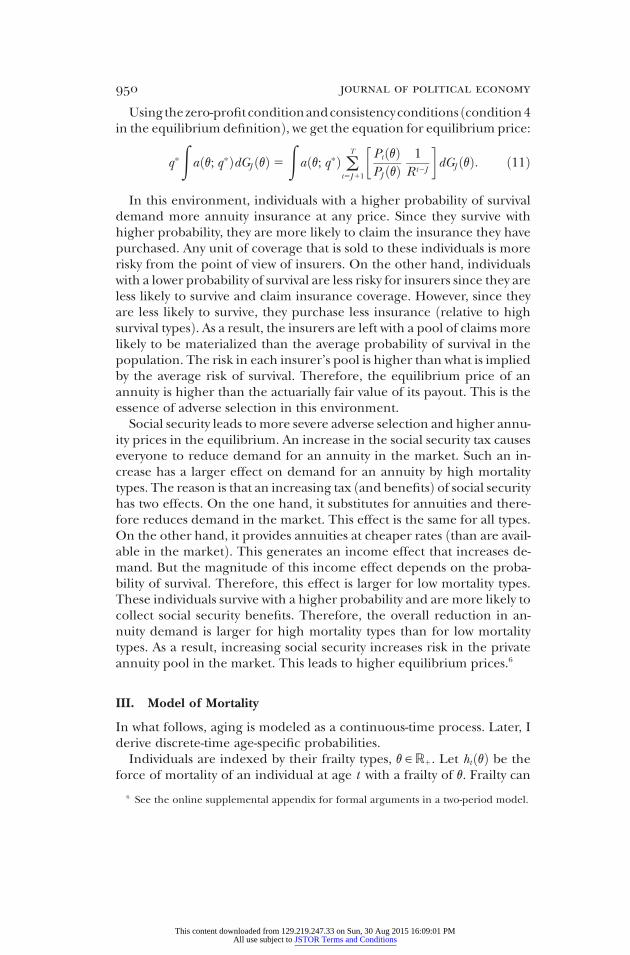
tion ð14Þ can be used to compute individuals’ survival probabilities P ðvÞ.Computed survival probabilities and their implied life expectancies areplotted in figure 1. The top panel shows the probability of survival to eachage. The bottom panel shows the implied life expectancy at each age. Sincefrailty is not observable, interpreting the degree of heterogeneity fromthe variance of the initial distribution of frailty is not straightforward. How-ever, heterogeneity in frailty implies heterogeneity in life expectancy ateach age. The estimation implies a standard deviation of 6 years for lifeexpectancy at age 30, which indicates a large degree of heterogeneity. Asa comparison, note that the gap in life expectancy between males and fe-males at age 30 for the birth cohort of 1930 is 5 years ðBell and Miller 2005,table 11Þ. Another comparison can be the gap in life expectancy betweencollege-educated and less than high school–educated males at age 25,which is about 6 years ðRichards and Barry 1998Þ. In what follows, I assumethat these subjective probabilities are true probabilities and represent thetrue risk of survival for each frailty type.

B. Annuitized Wealth at Retirement

I use the data on individual and household wealth and income in wave 7of the HRS ðyear 2004Þ to document the amount of annuitized wealth



held by respondents.8 I then calculate, on average, what fraction of in-dividuals’ retirement wealth ðdefined belowÞ is in the form of private an-

FIG. 1.—The top panel shows the probability of survival to each age. The bottom panelshows life expectancy at each age. Solid lines represent values for all the population.Dashed lines represent values for different quantiles of frailty, v.


nuities and defined-benefit pensions. This is used as a calibration targetin Section IV.C.

1. Annuitized Wealth in the HRS

I restrict my sample to male respondents who are older than 60 and col-lecting social security retirement benefits in wave 7. I use self-reporteddata on pension and annuity income as well as social security retirementbenefits to compute the expected present discounted value of annuities/pension and social security benefits. To discount future payments, I usepopulation survival probabilities for males of the 1930 birth cohort ðBelland Miller 2005, table 7Þ and a real interest rate of 3 percent. From nowon, I refer to these calculated present values as annuity and pension wealthand social security wealth, respectively.The HRS also collects data on household wealth, which includes fi-

nancial assets, housing equity, and other assets. Financial assets includeindividual retirement account ðIRAÞ balances; stock and mutual fund

8 The reason for choosing wave 7 is that this is the period in which most of the re-spondents in wave 1 become early retirees and start collecting social security and pension/
annuity income.


values; bond funds; checking, savings, money market, and certificates ofdeposit account balances; and trusts, less unsecured debt.Housing equity


is the value of the home less mortgages and home loans. Other assetsinclude the net value of other estates, vehicles, and businesses. I constructtotal retirement wealth for each individual as the sum of social securitywealth, annuity and pension, and wealth data reported in the HRS.9 I re-fer to this sum as retirement wealth. For each observation, I calculate whatfraction of retirement wealth is annuitized through social security, pri-vate annuities, or employer-provided defined-benefit pensions. I reportthe average of this fraction over all individuals in table 1 ðI calculate thisfraction for each observation and report the average over all observa-tionsÞ. The figures are similar for both married and single individuals.10

These numbers indicate that, on average, 10 percent of retirementwealth takes the form of private annuities or employer-provided defined-benefit pensions for males 60 years and older in wave 7 of the HRS. How-ever, only a small fraction of annuitized wealth takes the form of privateannuity contracts that people actively purchase using their accumulatedretirement assets.Table 2 shows the fraction of individuals in the sample who report pos-

itive annuity or defined-benefit pension income. As seen in columns 3and 6 in table 2, there is a significant fraction of individuals in the sam-ple ðabout halfÞ who receive annuity income either through private annu-ities that they have purchased using their accumulated retirement assetsor through employer-sponsored defined-benefit pension plans.In summary, tables 1 and 2 show that individuals, on average, have a

nontrivial amount of annuitized wealth, other than social security, at re-tirement. Also, a significant fraction receive annuity income from sourcesother than social security. However, table 2 also highlights a well-knownfact that only a small fraction of people actively buy private annuitycontracts. Most persons who receive annuity income other than social se-curity get the annuity through employers’ defined-benefit pension plans,which are in fact group annuity insurance arrangements purchased byemployers on their behalf. Also, table 1 shows thatmost annuitized wealthother than social security is held in the form of defined-benefit pensionentitlements.

2. Lump-Sum Withdrawals in Defined-Benefit Pension Plans

Workers who have a defined-benefit pension plan through their employ-ers have limited control over the amount of benefits to which they are

9
For HRS wealth data I use total wealth including secondary residence as reported inRAND HRS data, version M.
10 See the online supplemental appendix for the complete table by age andmarital status.



entitled.11However, a large fractionof theseworkersnowhaveanoption toclaim benefits in the form of an annuity ðdefault optionÞ or lump-sum

TABLE 1Average Fraction of Retirement Wealth That Is Annuitized

Employer-SponsoredPensions ð%Þ

ð1Þ

PrivateAnnuities ð%Þ

ð2Þ

SocialSecurity ð%Þ

ð3ÞAll 9.5 .5 34.560–64 11.8 .3 41.265–69 11.0 .3 37.070–74 10.4 .6 37.575–79 8.8 .7 33.2801 6.0 .7 26.4

Source.—Author’s calculations using wave 7 of RAND HRS data,version M.Note.—All calculations are for male respondents who are older

than 60 and collecting social security retirement benefits in wave 7.

TABLE 2Fraction of Population with a Private Annuity or a Defined-Benefit Pension

In Their Own Name ð%Þ In Own or Spouse’s Name ð%ÞEmployer-SponsoredPension

ð1Þ

PrivateAnnuity

ð2Þ

Pension orAnnuity

ð3Þ

Employer-SponsoredPension

ð4Þ

PrivateAnnuity

ð5Þ

Pension orAnnuity

ð6ÞAll 45.6 4.8 48.0 51.5 6.2 53.960–64 40.0 1.8 40.5 51.5 6.2 53.965–69 41.8 2.5 42.9 47.5 3.3 48.770–74 46.0 4.5 48.5 52.6 6.1 54.975–79 49.7 5.6 52.7 56.7 7.0 59.7801 48.9 8.8 52.9 54.4 10.8 58.7

Source.—Author’s calculations using wave 7 of RAND HRS data, version L.Note.—All calculations are for male respondents who are older than 60 and collecting

socials security retirement benefits in wave 7.


withdrawals ðof the present discounted value of annuity benefitsÞ. Thereis overwhelming evidence from a variety of sources that a significant frac-tion of defined-benefit pension plans allow for lump-sum withdrawal ofbenefits, and their number is growing. According to the US Departmentof Labor ð1995Þ, the fraction of defined-benefit participants with accessto any type of lump-sum option grew from 14 percent to 23 percent be-tween 1991 and 1997. In 2005, 52 percent of all private industry work-ers with defined-benefit pension plans had lump-sumwithdrawal optionsavailable to themat retirement ðUSDepartment of Labor 2007Þ. Burman,

11 The annuity benefit usually is based on an employee’s average salary and length of ser-vice with the employer. With each year of service, a worker accrues a benefit equal to either a
fixeddollaramountpermonthor yearof serviceorapercentageofhisorherfinal averagepay.


Coe, and Gale ð1999Þ report that on the basis of a 1993 employee bene-fit survey of the Current Population Survey, 58 percent of workers with


defined-benefit pensions were eligible for a lump-sum distribution. Fi-nally, Hurd and Panis ð2006Þ study the 1992–2000 waves of the HRS andfind that, on the basis of self-reported data, about 48 percent of full-time workers in the private sector had the option of lump-sum withdraw-als upon job separation.12 Perhaps more importantly, Hurd and Panisshow that a large fraction of individuals choose to receive benefits as anannuity when they are presented with the lump-sum withdrawal optionð24 percent expect to receive future annuity benefits, 56.2 percent drawcurrent benefits, and about 15 percent cash out or roll their accruedbenefits into an IRAÞ. Benartzi, Previtero, and Thaler ð2011Þ analyzemore than 103,000 payout decisions from 112 different defined-benefitplans provided by a large plan administrator between 2002 and 2008.They find that 49 percent of participants who retire between ages 50and 75 with at least 5 years of job tenure and account balances of $5,000chose to collect benefits as annuities when they were given the option oflump-sum withdrawals.This evidence suggests that a significant fraction of workers who re-

ceived annuity income through defined-benefit pension plans are facedwith the choice of collecting benefits as an annuity or a lump sum. Thereis little information on whether annuities offered in defined-benefitplans are more or less attractive than those offered on the market. How-ever, the Internal Revenue Code regulates conversion between lifetimeincome benefits and lump sums in defined-benefit pension plans byprescribing mortality tables and discount rates to use in the calculations.Benartzi et al. ð2011Þ show that the amount of ðminimumÞ lump-sumwithdrawals offered through these plans is comparable to the cost of thepurchase of annuities with similar payments. This means that financialcalculations made by these individuals are very similar to those of a pur-chase of an annuity contract. An important difference, however, is thatin almost all plans, receiving benefits as an annuity is the default option.This may be an important factor in deciding whether to receive incomeas an annuity or a lump sum ðhowever, as argued above, a nontrivial frac-tion of workers do choose to take lump-sum withdrawalsÞ. Also, althoughthe number of plans that offer lump-sum withdrawal options is grow-ing, there are still plans that offer no such options at retirement. ðHow-ever, almost all plans offer lump-sum withdrawals when workers quittheir jobs.Þ

12 Not all of these job separations are due to retirement. A portion of them are due to job
changes. However, depending on the size of benefits accrued and whether the worker isvested in the plan or not, she or he does have the option of making lump-sum withdrawalsor leaving the accrued benefit as is and receiving annuity income at retirement.


The model described in Section II is very simple and stylized in manyrespects. The only source of annuity income other than social security


in that model is the purchase of private annuity contracts. Motivated bythe discussion above, I compare annuity insurance that is purchased inthe model to the sum of private annuity and defined-benefit pensionincome in the HRS data. This is a simple way to account for all annu-ity income that individuals have without significantly complicating themodel.13

C. Benchmark Calibration

The model period is 5 years. Individuals enter the model at age 30, andno one survives past 110. All individuals are endowed with the samehump-shaped earnings profile between ages 30 and 65, when they all re-tire. I use the US cross-sectional labor endowment efficiency profile esti-mated by Hansen ð1993Þ.The utility function is constant relative risk aversion with coefficient of

risk aversion g over consumption and bequests:

uðcÞ5 c12g

12 gand vðbÞ5 y

b12g

12 g:

The term y > 0 is the weight on the bequest in the utility function and isidentical for every individual. The higher y is, the higher the value of thebequest for individuals and the lower the demand for annuities.For the curvature parameter of the utility function, g, I use a bench-

mark value of g5 2 and explore alternative values of g5 1 and g5 4 inSection VI.A. The annual discount factor is b5 0:97 and the annual realinterest rate is 3 percent. Equation ð8Þ is used to find social security taxesand benefits that match an average replacement rate of 45 percent.14

Finally, to find the weight on the bequest, I solve the model using sur-vival profiles calculated in Section IV.A and choose y such that, on av-erage, the annuity wealth in the model is equal to 10 percent of total re-tirementwealth. Tomaintain consistency with calculations in the data, thepresent discounted values of annuity and social security income in themodel are calculated using population survivals ðrather than individualsurvivalsÞ.Table 3 shows the calibrated parameters. All parameters other than g

and y will remain unchanged across various experiments and robustness

13 I have also performed calibration and welfare calculations under three alternativeassumptions. The results are reported in the online supplemental appendix.

14 I assume that returns on social security are the same as market returns ð3 percent an-nuallyÞ in the fully funded system I consider. This implies that a lower tax rate is required tobalance the budget, relative to what is usually found under a pay-as-you-go system ðin whichreturns are tied to demographic parametersÞ.



exercises. Slightly more than half of the individuals hold an annuity atretirement in the model. This is in line with evidence reported in table 2.

TABLE 3Benchmark Calibration

Parameter Description Value Notes

T Maximum age 17 Real life age of 110–114J Retirement age 7 Real life age of 60–65wt Earnings profile Taken from Hansen ð1993Þb Discount factor .97 AnnualR Real returns 1.03 Annualg Risk aversion parameter 2 Benchmark value*jv Standard deviation of logð9Þ .56 Estimated using HRS response of

subjective survival probabilitiesðsee the AppendixÞ

PtðvÞ Individual survivals Constructed to match life table forthe 1930 birth cohort ðeq. ½18�Þ

t Social security tax .08 Finance social security replacementrate of .45

y Weight on bequest .9 Average annuitized wealth atretirement 5 10%

Note.—The fraction with an annuity ðnot targetedÞ is 0.53.* See Sec. VI.A for sensitivity.


It shows that the model does a reasonable job of matching the actual rateof annuitization in the HRS data.

V. Findings

The main goal of the quantitative exercise is to find how much welfareis gained, ex ante, from implementation of mandatory annuitization inthe current US social security system. I also report what would be welfaregains from implementing the ex ante efficient allocation described inSection II.B. The first calculation serves as a benchmark for how success-ful the current US social security system is inmitigating adverse selection.The second calculation is a benchmark for how much could possibly begained.To highlight the role of market structure in my calculations, I per-

form the quantitative exercise under three different assumptions as de-scribed below.Economy with no survival-contingent assets.—This is an economy without

any annuity contracts. Individuals can accumulate noncontingent as-sets only at rate R, which they leave as bequests if they die. I refer to thisarrangement as autarky. If there is no social security, there will be nosurvival risk sharing in this economy. Note that in this economy the sup-ply of annuity contracts is exogenously fixed at zero. So there will be nomarket response to a policy. Only individual consumption and saving al-locations are different across scenarios with and without social security.



Economy with annuity markets and full information.—This is similar to themodel economy described in Section II with the exception that the price


of the annuity contract is assumed to be actuarially fair for each type. Inother words, type v pays the price qAF ðvÞ, which is the actuarially fair valueof the unit annuity coverage that he purchases. I refer to this arrange-ment as an annuity market with full information. Note that in this economythe price of an annuity for each person is determined by his mortalityrisk type v. Therefore, only the demand for annuity coverage ðand not itspriceÞ will be affected by social security policy.Economy with annuity markets and private information.—This is the full-

blown model economy described in Section II. Individuals can purchasean annuity at the period before retirement. However, because of pri-vate information, there is adverse selection in the annuity market andthe price is not actuarially fair. I refer to this arrangement as an annuitymarket with private information. In this economy the participation in theannuity market and the price of private annuity contracts depend on thelevel of social security tax and benefits.I solve the model under all three assumptions above and calculate the

ex ante welfare difference between the economy without social securityand the economy with the current US replacement ratio. I calculate wel-fare as the percentage increase in lifetime income an individual requires,ex ante, without social security in order to be as well off as with socialsecurity.

A. Welfare Gains from the Current US System

Table 4 shows ex ante welfare gains from the current US replacementratio relative to an economy without social security. The first row showsthe welfare gain under the autarky assumption. As is expected in this case,the welfare gain is large since social security is the only source for annuityincome at retirement.The second row shows the welfare gain under the assumption of full

information. As is expected, the welfare gain from social security is smallin this case since every individual has access to an actuarially fair annuity.

TABLE 4
Benchmark Welfare Calculations: Ex Ante Welfare Gains
from Annuitization in the Current US System

Welfare Gain ð%ÞAutarky 2.68Annuity market with full information .01Annuity market with private information .07Annuity market with private information ðwith annuity prices fixedÞ .42

Note.—Welfare gains are reported relative to an economy without social security.



The third row shows the main welfare calculation. That is the welfaregain from the current US replacement ratio under the assumption that


mortality types are private information and there is adverse selection inthe annuity market. Note that this number is much smaller than that inthe first row. There are three reasons for this. First, in contrast to theautarky case, in the absence of social security, individuals can purchasean annuity in theprivate annuitymarket. Therefore, the outcomewithoutsocial security is not as bad as in the autarky case. Second, as is the casewith any forced insurance, individuals with low risk suffer losses. This willreduce the ex ante welfare gain from the policy. Third, social securitycrowds out good risk types ðhighermortality typesÞ in the annuitymarket.This leads to more severe adverse selection and increases in the marketprice of private annuities in the presence of social security. In fact, themarket price of private annuities is 14 percent higher in the economywiththe current US replacement ratio relative to an economy without socialsecurity.15 To highlight the importance of this price effect, the fourthrow reports welfare calculations under the private information assump-tion; but if the market price of annuities is held at that level, it wouldbe in an economy without social security. If prices are held fixed, welfaregains from the current US replacement ratio would be higher by about0.35 percent.This finding highlights the key message of the paper. In the absence of

social security, all individuals join the annuity market. In particular, thehigh-mortality individuals who are the good risk types will buy annuities.This leads to a better insurance pool, lower prices, and better risk shar-ing, ex ante. Public provision of annuities through social security crowdsout private annuity markets. In particular, it runs good risk types ðhighmortality typesÞ out of the markets. This in turn leads to high risks in theinsurance pool and high prices. The calculation above shows that theseprice effects can have sizable welfare implications. Comparison of wel-fare gains in the first and third rows shows that ignoring endogenousresponses of insurance markets to the policy can lead to very differentconclusions about the usefulness of the policy. This is also in line withresults by Golosov and Tsyvinski ð2007Þ and Krueger and Perri ð2011Þ,who study endogenous insurance markets and the welfare implicationsof crowding out of private insurance by public insurance.Figure 2 shows ex post welfare gains/losses by frailty type v. The thick

black line is the welfare gain from the current US replacement ratiounder the assumption of annuity markets with private information. Wel-fare gains are positive and small for 80 percent of the population. The

15 This finding is not new. Walliser ð2000Þ also finds that in the absence of social security,annuity prices would be lower, although he reports much smaller numbers ð2–3 percentÞ.
Part of the reason is that the annuity contracts he considers are not life annuities. Insteadthey are one-period survival-contingent bonds.


20 percent with the highest mortality do not gain. In fact they suffer bigwelfare losses. These are individuals who have little value for annuitiza-

FIG. 2.—Ex post welfare gains/losses from the current US system relative to an economywith no social security for various assumptions regarding annuity markets.


tion, would rather not pay social security taxes, and instead increase theirconsumption at younger ages. The gray dashed line shows the same cal-culation but with the annuity price fixed at the level it would be whenthere is no social security. In this case welfare gains are higher for lowerfrailty types. This highlights the fact that the effect of social security onannuity prices ismost harmful for the lowestmortality types.These are therisk types who value annuities most.The dashed and dotted line and the dotted line show welfare gains

under autarky and full information, respectively. Gains under autarkyare significantly higher for lower mortality types and vanish as we movetoward higher mortality types. Finally, gains and losses under the full-information assumption almost offset each other. But even under full in-formation, some individuals make huge gains from social security andalmost equal numbers suffer huge losses ðthese gains and losses are dueto cross-subsidies across mortality typesÞ.The results presented so far report only how useful current US social

security is in mitigating adverse selection in the annuity market. Theupshot from these findings is that social security has little welfare gain exante ðand ex postÞ, mainly because it lowers the welfare of high mortalitytypes and worsens the adverse selection problem in the market for lowmortality types. These results, however, do not mean that the welfare cost



of private information in annuity markets is small. Nor do they necessar-ily mean that annuity markets provide large benefits ðover the autarky


alternativeÞ.To assess the cost of private information in the annuity market, table 5

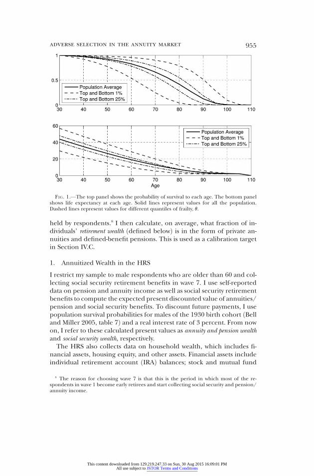
reports the ex ante welfare difference between an economy with full in-formation and an economy with private information. This is the percent-age increase in lifetime income that individuals require in the privateinformation economy in order to be as well off as in the full informationeconomy. The calculation is done both with and without the current USsocial security replacement ratio. The ex ante cost of private informationis about 0.38 percent.Table 6 shows the ex ante welfare benefit of having access to an an-

nuity market with private information relative to autarky. This is the per-centage increase in lifetime income individuals require in the autarkyeconomy in order to be as well off as in the economy with annuity mar-kets and private information. This is a measure of how useful the annu-ity market is in providing longevity risk sharing. As is expected, the an-nuity market is more valuable when there is no social security ðand hencethere is no alternative source for annuitized incomeÞ. The value of theannuity market is 2.79 percent in the economy without social securityand 0.17 percent in the economy with the current US social security re-placement ratio. This shows that in this model, in the absence of socialsecurity, a substantial amount of survival risk can be shared through theprivate annuity market, even though the market suffers from inefficien-cies due to adverse selection.

B. Optimal Policy

I discuss two benchmarks for optimal policy. In the first part I keep thepolicy instrument as before, that is, an age-independent tax rate duringworking ages and a constant social security benefit after retirement. Ithenfind the best combination of tax and benefits thatmaximizes ex antewelfare. In the second part I remove restrictions on policy and discuss im-plementation of ex ante efficient allocations discussed in Section II.B.

TABLE 5
Cost of Private Information: Welfare Losses
Due to Private Information

Welfare Loss ð%ÞWithout social security .38With social security .32

Note.—This table reports the welfare difference betweenan economy with an annuity market and private information,and an economy with an annuity market and full information.



1. Optimal Social Security Tax and Retirement Benefit

TABLE 6Value of an Annuity Market: Welfare Gains from

Having Access to an Annuity Market

Welfare Gain ð%ÞWithout social security 2.79With social security .17

Note.—This table reports the welfare difference betweenan economy with an annuity market and private information,and an autarky economy.


Table 7 shows the optimal replacement ratio and tax and ex ante welfaregains associated with them under the three assumptions regarding mar-kets ðautarky, full information, and private informationÞ. In all cases wel-fare gains are reported relative to an economy without social security.Recall that in the calibration the social security replacement ratio is 45 per-cent. Column 1 in table 7 shows optimal replacement ratios. The optimalreplacement ratio under the autarky assumption is much higher than inthe two other cases. In fact, when annuity markets are present ðboth withfull information and with private informationÞ, optimal replacement ra-tios are smaller than 45 percent ðthe benchmark calibrated value for thecurrent US systemÞ. The reason is that in this model there is a consider-able demand for life insurance ðsurvival benefitsÞ at younger ages whenindividuals have few assets. A lower replacement ratio means lower taxes.Lower taxes allow individuals to accumulate assets faster, which they canleave as bequests if they die young. This is not a big concern in older agessince after retirement individuals can purchase an annuity ðor receive so-cial securityÞ, which insures one side of their mortality/survival risk.

2. Implementing Ex Ante Efficient Allocation

In this section I relax the restriction on policy instruments and describea simple policy to implement ex ante efficient allocations in this model

TABLE 7
Optimal Social Security Tax and Retirement Benefit
OptimalReplacement

Ratioð1Þ

Optimal Taxð2Þ

Welfare Gainð%Þð3Þ

Autarky .58 .10 2.83Annuity market with full information .24 .04 .10Annuity market with private information .29 .05 .08

Note.—Welfare gains are reported relative to an economy without social security.



and report welfare gains from implementing these allocations. I refer tothese allocations and the policy that implements them as first-best.


Recall from Section II.B that an ex ante efficient allocation is inde-pendent of mortality type. Everyone receives the same allocation inde-pendent of type. Also, the allocation must satisfy

u 0ðctÞ5 bRu 0ðct11Þ5 bRv 0ðbtÞ;in which bt is the bequest left if the individual dies at the end of age t.I will maintain the assumption that bR 5 1; hence allocations are con-stant over age. Let ðc*, b*Þ be the ex ante efficient level of consumptionðcontingent on survivalÞ and bequest ðcontingent on deathÞ. I propose asystem of a social security tax rate, t*, a social security retirement benefit,z*, and a sequence of survival benefits ðl *0 ; l *1 ; : : :; l *T Þ that pays l *t if theindividual dies at the end of age t. Consider the consumer problem ofSection II.C.2 with the proposed social security policy

maxct ;bt ;kt11;a ≥ 0 o

T

t50

PtðvÞbtfuðctðvÞÞ1 ½12 xt11ðvÞ�bvðRkt11ðvÞ1 l *t Þg

subject to

ct 1 kt11 5 Rkt 1 ð12 t*Þwt for t < J ;

cJ 1 kJ11 1 qa 5 RkJ 1 ð12 t*ÞwJ ;

ct 1 kt11 5 Rkt 1 a 1 z* for t > J ;

k 0 5 0:

Proposition 1. Suppose that bR 5 1 and let ðc*, b*Þ be the exante efficient level of consumption and bequest. A social security policyðt*; z*; l *t Þ such that

z* 5 c* 1�

1R

2 1�b*;

l *t 50 for t ≥ J

ð12 t*Þwt11 2 c* 1�12

1R

�b* 1

l *t11

Rfor t < J ;

8<:

and

E�oJt50

PtðvÞRt

12 xt11ðvÞR

l *t 1 oT

t5J11

PtðvÞRt

z*�dG0ðvÞ

5 t*EoJt50

PtðvÞRt

wtdG0ðvÞ

implements ðc*, b*Þ.



Proof. The goal is to show that taking the policy ðt*; z*; l *t Þ as given, anindividual will choose ðc*, b*Þ. I first show that for any type v, if an in-


dividual purchases zero annuity, he will choose allocation ðc*, b*Þ. ThenI show that given these choices, purchasing zero annuity is optimal. Con-sider the individual’s first-order condition

PtðvÞu 0ðctÞ5 Pt11ðvÞbRu 0ðct11Þ1 PtðvÞ½12 xt11ðvÞ�bRv 0ðRkt11ðvÞ1 l *t Þ:

Notice that if the individual chooses ctðvÞ5 c* and kt11ðvÞ5 ðb* 2 l *t Þ=R ,the first-order condition is satisfied since a property of allocation ðc*, b*Þis thatu 0ðc*Þ5 v 0ðb*Þ. Also, it is straightforward to check that these choicessatisfy consumers’ budget constraints and the government’s budget con-straints by construction.Now consider the following annuity price:

q 5 supvoT

t5J11

PtðvÞPJ ðvÞRt2J

:

With ctðvÞ5 c*, we have

qu 0ðcJ ðvÞÞ ≥ oT

t5J11

PtðvÞPJ ðvÞb

t2J u 0ðctðvÞÞ;

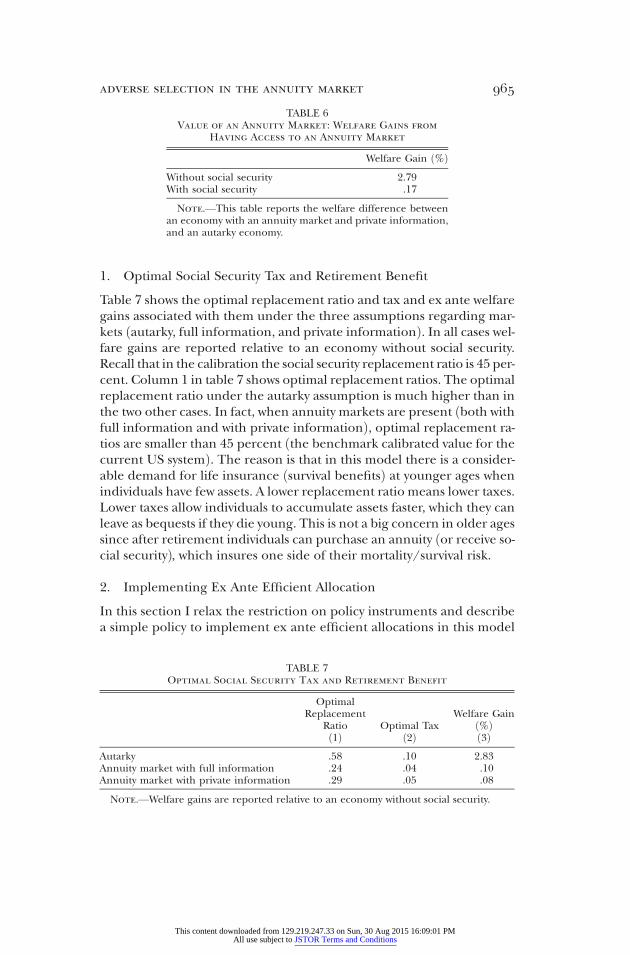
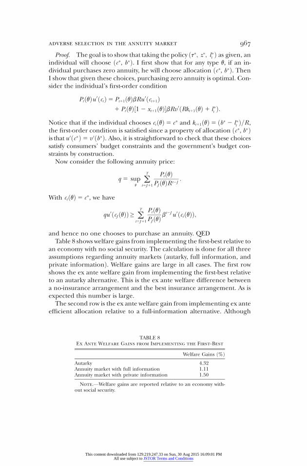
and hence no one chooses to purchase an annuity. QEDTable 8 shows welfare gains from implementing the first-best relative to

an economy with no social security. The calculation is done for all threeassumptions regarding annuity markets ðautarky, full information, andprivate informationÞ. Welfare gains are large in all cases. The first rowshows the ex ante welfare gain from implementing the first-best relativeto an autarky alternative. This is the ex ante welfare difference betweena no-insurance arrangement and the best insurance arrangement. As isexpected this number is large.The second row is the ex ante welfare gain from implementing ex ante

efficient allocation relative to a full-information alternative. Although

TABLE 8Ex Ante Welfare Gains from Implementing the First-Best

Welfare Gains ð%ÞAutarky 4.32Annuity market with full information 1.11Annuity market with private information 1.50

Note.—Welfare gains are reported relative to an economy with-out social security.



this number is much smaller than in the first row, it is still quite large. Itappears that even the annuity market with full information is far from


the first-best ðbut similarly far from autarkyÞ. This is, for the most part,the result of ignoring the life insurance market in the model.16

The third row shows the welfare gain from implementing the first-bestin the economy with an annuity market and private information. Thesenumbers are alsomuch smaller than those in the first row, which is an indi-cation that even an annuity market with private information goes a longway in providing survival risk sharing ðthis is also evident from table 6Þ.However, the fact that these welfare gains are large is also an indicationthat there is substantial uninsured survival risk ðand survival heteroge-neityÞ in the environment. Comparing these numbers with the third rowin table 4, we see that in the current US system the combination of socialsecurity and the annuity market is able to provide insurance that is wortha tiny fraction of the gain achievable under first-best ð0.06 vs. 1.50Þ.The left panel in figure 3 shows the policies that implement the first-

best. We can see that implementation requires large survival benefits atvery young ages. This highlights, once again, that part of these large wel-fare gains are due to life insurance aspects of first-best policies ðand notthe annuity aspect of itÞ.17The right panel in figure 3 shows ex post welfare gains for different

mortality types. About 95 percent of individuals gain from implement-ing ex ante efficient allocations ðin a private information economyÞ, andthese gains are significant for a large fraction of mortality types.

VI. Robustness

I explore robustness of the results presented in Section V. First, I exam-ine how choosing a different risk aversion parameter affects calibrationand welfare calculations. Calibration of bequest parameters and welfarenumbers is somewhat sensitive to the choice of risk aversion parameters.Second, I extend the model to include preference heterogeneity overbequests. The main findings of Section V are quite robust to this exten-sion. Finally, I introduce heterogeneity in earnings profiles. Althoughincome heterogeneity affects welfare numbers, it does not alter the mainconclusions.18

16 An active life insurance market together with the annuity market considered here can
get very close to the ex ante efficient allocation under full information.
17 Although social security provides survival benefits, these benefits are paid primarily tosurvivors of older/retired workers ðunless the survivor cares for a young childÞ. The survivalbenefits that come out of the first-best policy here are very different from those in the cur-rent US social security system. They are age dependent and are paid only to young workers.

18 The online supplemental appendix contains more robustness exercises with respectto various parameters and assumptions.



FIG.3.—

Theleftpan

elshowsthefirst-bestsurvival

ben

efitsan

dretiremen

tben

efitsrelative

tomeanearnings.Therigh

tpan

elshowsex

postwelfare


gains/losses

from

implemen

tingthefirst-bestrelative

toan

economywithnosocial

secu

rity

forthreeassumptionsregardingan

nuitymarke

ts.


A. Sensitivity to Risk Aversion Parameters


Before I present calibration and welfare calculations under different val-ues for risk aversion parameters, it is important to discuss how risk aver-sion affects equilibrium outcomes. The annuity price is higher in aneconomy with a lower risk aversion parameter.19 The intuition for thisresult is as follows. In an economy with a lower value of a risk aversionparameter, individuals have less desire for a smooth consumption profileand are more sensitive to intertemporal prices. In this model there arealways low-mortality individuals who find annuity prices lower than theactuarially fair price of their risk types. These individuals buy more annu-ity if risk aversion is lower. On the other hand, there are always individu-als with high mortality who find annuities to be more expensive than theactuarially fair price of their risk types. These individuals buy less annuityif risk aversion is lower. This implies that at lower risk aversion the dif-ference between the demand for annuity for high and low mortality ishigher; that is, the profile of annuity purchase is steeper. This leads to amore severe adverse selection problem and higher annuity prices. There-fore, for lower values of risk aversion, the annuity price is higher andannuities are less attractive. On the other hand, for higher values of riskaversion, annuity prices are lower and annuities are more attractive.The discussion above implies that to match the target of annuitized

wealth at retirement, the calibrated value of y ðthe bequest parameterÞmust be lower ðhigherÞ for lower ðhigherÞ risk aversion. Otherwise, therewill be too little or too much annuitization in the model. Table 9 showsthe calibration for three different values of risk aversion parameters,g5 1, 2, and 4. The bottom row shows the fraction of the populationwho buy an annuity in each case. For g5 1, the annuity market is theleast attractive of all. Therefore, only 41 percent purchase an annuity.This is still in line with data reported in table 2. For g5 4, the annuitymarket is very attractive and 69 percent purchase an annuity. For thiscase the model predicts too many individuals who purchase an annuity.Welfare calculations are presented in table 10. As is expected, welfare

gains from social security are higher for lower values of risk aversion. Forreasons discussed above, for g5 1, the adverse selection is more severe,and therefore, individuals will gain more, ex ante, from public provisionof annuities. Also, the calibrated value for y is lower, which means thatindividuals have more value for annuity income in general. For the samereasons, the cost of private information is also higher for g5 1 and thebenefit from access to annuity markets is lower.On the other hand, welfare gains from the current US system are neg-

ative for g5 4. Part of the reason is that annuity markets perform betterif risk aversion is higher, and therefore, the adverse selection problem is

19 The online supplemental appendix contains a formal proof for a two-period model.



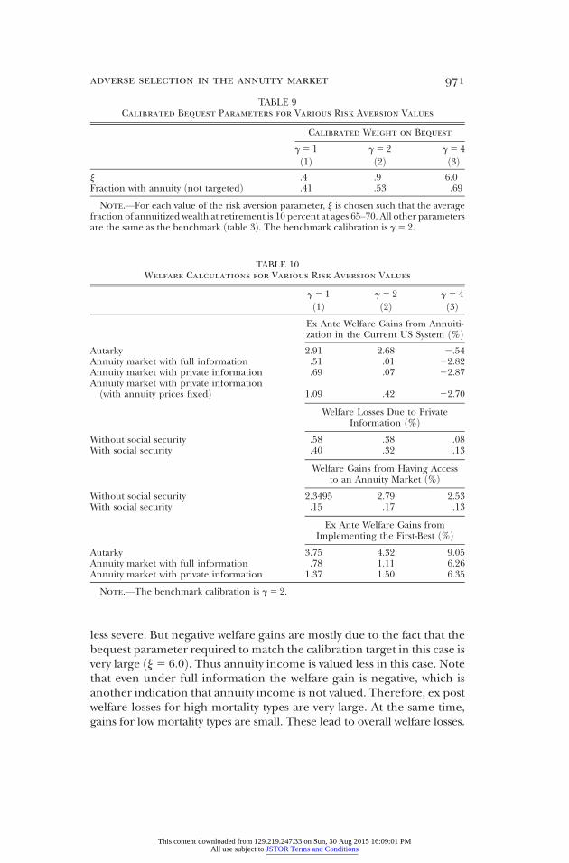
less severe. But negative welfare gains are mostly due to the fact that thebequest parameter required to match the calibration target in this case is

TABLE 9Calibrated Bequest Parameters for Various Risk Aversion Values

Calibrated Weight on Bequest

g5 1ð1Þ

g5 2ð2Þ

g5 4ð3Þ

y .4 .9 6.0Fraction with annuity ðnot targetedÞ .41 .53 .69

Note.—For each value of the risk aversion parameter, y is chosen such that the averagefraction of annuitized wealth at retirement is 10 percent at ages 65–70. All other parameterare the same as the benchmark ðtable 3Þ. The benchmark calibration is g5 2.

TABLE 10Welfare Calculations for Various Risk Aversion Values

g5 1ð1Þ

g5 2ð2Þ

g5 4ð3Þ

Ex Ante Welfare Gains from Annuitization in the Current US System ð%Þ

Autarky 2.91 2.68 2.54Annuity market with full information .51 .01 22.82Annuity market with private information .69 .07 22.87Annuity market with private informationðwith annuity prices fixedÞ 1.09 .42 22.70

Welfare Losses Due to PrivateInformation ð%Þ

Without social security .58 .38 .08With social security .40 .32 .13

Welfare Gains from Having Accessto an Annuity Market ð%Þ

Without social security 2.3495 2.79 2.53With social security .15 .17 .13

Ex Ante Welfare Gains fromImplementing the First-Best ð%Þ

Autarky 3.75 4.32 9.05Annuity market with full information .78 1.11 6.26Annuity market with private information 1.37 1.50 6.35

Note.—The benchmark calibration is g5 2.



s

-

very large ðy5 6:0Þ. Thus annuity income is valued less in this case. Notethat even under full information the welfare gain is negative, which isanother indication that annuity income is not valued. Therefore, ex postwelfare losses for high mortality types are very large. At the same time,gains for low mortality types are small. These lead to overall welfare losses.


The gains from implementing the first-best, however, are large in thiscase. As discussed in the previous section, the first-best has an important


life insurance component that is highly valued if risk aversion is g5 4 andthe bequest parameter is y5 6:0.In all cases welfare gains from annuitization in the current US system

are much smaller in the economy with annuity markets and privateinformation relative to autarky. Also, the crowding-out effect of social se-curity on prices is significant in all cases. For example, without the effecton prices, the welfare gain would have been more than 1 percent in theg5 1 case.

B. Heterogeneity in Preferences

I extend the model to include heterogeneity in the bequest parameter,y, as well as heterogeneity in mortality. The model that I solve is verysimilar to the model in Einav et al. ð2010Þ. To capture possible correla-tion between the bequest parameter y and the mortality parameter v, Iassume that they are joint lognormal with correlation coefficient r:

�logðvÞlogðyÞ

�∼N

��0my

�;

�j2v

rjvjy

rjvjy j2y

��:

For marginal distribution of v, I assume the same parameters as esti-mated in the Appendix and reported in table 3. I use the estimation ofEinav et al. for jy and r and calibrate the mean parameter my to matchthe average fraction of wealth annuitized at retirement ðsimilar to thecalibration of the strategy in Sec. IV.CÞ. The risk aversion parameter isequal to the benchmark value of g5 2. Table 11 shows the calibrated

TABLE 11Calibration Summary for Preference Heterogeneity

Calibrated Average ðLog ofÞWeight on Bequest

jy 5 :099,r5 :88ð1Þ

jy 5 :198,r5 :88ð2Þ

jy 5 :099,r5 :088

ð3Þ

jy 5 0r5 0ð4Þ

my ðmean of ½log�bequest parameterÞ 2.07 2.03 2.1 2.1

Fraction with annuityðnot targetedÞ .52 .51 .53 .53

Note.—The risk aversion parameter in all cases is g5 2. The weight is chosen to matchaverage annuitized wealth of 10 percent at ages 65–70. In col. 1, jy 5 :099 is the estimationfrom Einav et al. ð2010Þ. The benchmark calibration is jy 5 0.


,


mean parameter my. All other parameters are fixed at the values reportedin table 3.


Column 1 of table 11 uses the benchmark estimation in Einav et al.ð2010Þ for jy and r. These are estimated as jb and r in their table 3.Column 2 uses the same value for r as column 1, but with a jy that is twiceas large.Column3uses the same value for jy as column 1, but with r 10 timessmaller. Finally, column 4 is the benchmark calibration discussed in Sec-tion IV.C. In all specifications the average annuitized wealth of 10 percentis matched. And the average values for the parameter y are close to 0.9in all cases. Also, in all specifications, close to half of the population pur-chase annuities.Table 12 presents a summary of all welfare calculations discussed in

the previous section. All welfare numbers are very close to the numbersfound in the benchmark model.Note that with preference heterogeneity, the ex ante efficient ðthe

first-bestÞ allocations are no longer uniform across types. Therefore, theyare not incentive compatible and cannot be implemented with type-independent policies. On the other hand, characterizing and implement-ing the ex ante efficient allocation in an economy with heterogeneity andmultidimensional private information is a difficult problem and is out-side the scope of this paper. Therefore, the ex ante efficient ðor first-bestÞ

TABLE 12Welfare Calculations with Preference Heterogeneity

jy 5 :099,r5 :88ð1Þ

jy 5 :198,r5 :88ð2Þ

jy 5 :099,r5 :088

ð3Þ

jy 5 0r5 0ð4Þ

Ex Ante Welfare Gains from Annuitizationin the Current US System ð%Þ

Autarky 2.62 2.53 2.67 2.68Annuity market with full information 2.03 2.06 .00 .00Annuity market with private information .06 .04 .06 .07Annuity market with private informationðwith annuity prices fixedÞ .40 .37 .41 .42

Welfare Losses Due to Private Informationð%Þ

With social security .39 .40 .38 .39Without social security .30 .29 .32 .32

Welfare Gains from Having Accessto an Annuity Market ð%Þ

With social security 2.73 2.67 2.78 2.76Without social security .17 .17 .17 .17

Note.—The risk aversion parameter in all cases is g5 2. In col. 1, jy 5 :099 is theestimation from Einav et al. ð2010Þ. The benchmark calibration is jy 5 0.


,


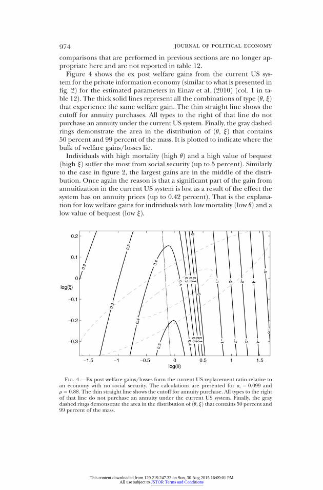
comparisons that are performed in previous sections are no longer ap-propriate here and are not reported in table 12.


Figure 4 shows the ex post welfare gains from the current US sys-tem for the private information economy ðsimilar to what is presented infig. 2Þ for the estimated parameters in Einav et al. ð2010Þ ðcol. 1 in ta-ble 12Þ. The thick solid lines represent all the combinations of type ðv, yÞthat experience the same welfare gain. The thin straight line shows thecutoff for annuity purchases. All types to the right of that line do notpurchase an annuity under the current US system. Finally, the gray dashedrings demonstrate the area in the distribution of ðv, yÞ that contains50 percent and 99 percent of the mass. It is plotted to indicate where thebulk of welfare gains/losses lie.Individuals with high mortality ðhigh vÞ and a high value of bequest

ðhigh yÞ suffer the most from social security ðup to 5 percentÞ. Similarlyto the case in figure 2, the largest gains are in the middle of the distri-bution. Once again the reason is that a significant part of the gain fromannuitization in the current US system is lost as a result of the effect thesystem has on annuity prices ðup to 0.42 percentÞ. That is the explana-tion for low welfare gains for individuals with low mortality ðlow vÞ and alow value of bequest ðlow yÞ.

FIG. 4.—Ex post welfare gains/losses form the current US replacement ratio relative toan economy with no social security. The calculations are presented for je 5 0:099 andr5 0:88. The thin straight line shows the cutoff for annuity purchase. All types to the righof that line do not purchase an annuity under the current US system. Finally, the graydashed rings demonstrate the area in the distribution of ðv, yÞ that contains 50 percent and99 percent of the mass.


t


C. Heterogeneous Earnings Profiles


So far I have maintained the assumption that all individuals have thesame age-varying profile of earnings. Although individuals will choosedifferent levels of savings and therefore have different assets when theyretire, there is no heterogeneity in their earnings ability in the model.This assumption was chosen to simplify the environment and focus onthe annuitization and cross-insurance across mortality types rather thanredistributional effects across income types. In this section I introduceincome heterogeneity in a very simple and tractable way that also allowsme to incorporate the correlation between mortality and income.To maintain comparability with previous sections, I continue to as-

sume the same distribution for mortality type v. I also assume no hetero-geneity in preferences ðas in the benchmark calibrationÞ and assume riskaversion of g5 2. Heterogeneity in earnings is introduced by assumingthat individuals have earnings e � wt , where wt is the same common hump-shaped earning profile used in the previous sections of the paper ðtakenfrom Hansen ½1993�Þ and e is an age-independent scale factor. The scalefactor e has a lognormal distribution with mean zero and standard de-viation je. I assume that v and e have the following joint distribution:

�logðvÞlogðeÞ

�∼N

��00

�;

�j2v

rejvje

rejvje j2e

��:

To calibrate parameters of income heterogeneity, I choose je to matcha Gini coefficient of earnings equal to 0.5, which is the average value forearnings of prime-age workers ðBudrıa et al. 2011Þ. I then choose the cor-relation parameter re to match mortality ratios by income quintile as re-ported in Cristia ð2009Þ.20 These mortality ratios measure the likelihoodof death for a person in a particular income group relative to the averagepopulation of the same age. The mortality ratios calculated by Cristia formen aged 50–64 are presented in table 13 ðcol. 2Þ. For example, column 2indicates that amale between ages 50 and 64 who is in the bottom incomequintile is 1.63 timesmore likely to die than a randomperson of the sameage in the population.Given the standard deviation on earnings je and mortality jv, I choose

the correlation re to minimize the distance between the mortality ratioin the model and data. The fit of the model is reported in table 13. Oncethe parameters of the joint distribution of ðv, eÞ are known, I use themodel to calibrate y by matching the average fraction of wealth that isannuitized at retirement. The target value is 10 percent as in previous

20 He uses data from the 1984, 1993, 1996, and 2001 panels of the Survey of Income andProgram Participation, matched to several files administered by the Social Security Admin-
istration. See Cristia ð2009Þ for details on data and calculations of mortality ratios.


ections. Table 14 shows the calibrated parameters as well as the fractionf the population who hold annuities. As was the case in previous sec

redistributing heterogeneous income. It is, however, interesting to investigate an environment when both income ðor abilityÞ and mortality are private information. This is left for future research.

TABLE 13Calibration of Income Mortality Correlation:

Mortality Ratios for Men Aged 50–64

Modelð1Þ

Datað2Þ

Bottom income quintile 1.62 1.632nd income quintile 1.17 1.103rd income quintile .95 .994th income quintile .77 .68Top income quintile .55 .61

Note.—Data in col. 2 are taken from table 2 in Cristia ð2009Þ.

TABLE 14Model Calibration with Income Heterogeneity: Parameters for

Earnings Profiles and Weight on Bequest

Parameter Value Notes

je .95 Earnings Gini of .45re 2.79 Match mortality ratio by income quintile*y .37 Average fraction of wealth annuitized 5 10%

Note.—The risk aversion parameter in all cases is g5 2. The fraction with anannuity ðnot targetedÞ is .53.* Taken from table 2 in Cristia ð2009Þ.



-
so tions, this fraction is in line with data in table 2.Table 15 shows the results of the main welfare calculations, that is, ex
ante welfare gains from the current US social security system.21 Column 1shows welfare numbers in the model with the heterogeneous earningsprofile. Column 2 shows results in the benchmark calibration. Note thatin the economy with annuity markets ðboth with full information andwith private informationÞ, welfare gains from the current US system arenegative. Low mortality types in this economy are more likely to be poor.Therefore, they suffer more from paying taxes while young, especiallysince the likelihood of receiving benefits is low ðbecause of their highmortalityÞ. In this economy social security will redistribute from poor andhigh-mortality individuals to rich and low-mortality individuals.These numbers indicate that the main finding of the paper is not sen-

sitive to adding earning heterogeneity to the model. Still there is a largecrowding-out effect from social security, which significantly reduces itspotential gains. On top of that, when there is heterogeneity in earnings,

21 Other calculations in this case are not very informative. For example, it is obvious thatwelfare gains from implementing the first-best are huge. But most of the gain comes from

--


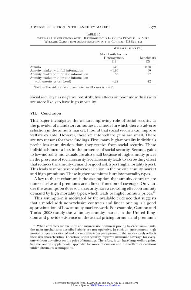
ocial security has negative redistributive effects on poor individuals whore more likely to have high mortality.

TABLE 15Welfare Calculations with Heterogeneous Earnings Profile: Ex Ante

Welfare Gains from Annuitization in the Current US System

Welfare Gains ð%ÞModel with Income

Heterogeneityð1Þ

Benchmarkð2Þ

utarky 1.20 2.68nnuity market with full information 21.90 .00nnuity market with private information 2.35 .07nnuity market with private informationðwith annuity prices fixedÞ 2.22 .42

Note.—The risk aversion parameter in all cases is g5 2.


sa

AAAA

VII. Conclusion

This paper investigates the welfare-improving role of social security asthe provider of mandatory annuities in a model in which there is adverseselection in the annuity market. I found that social security can improvewelfare ex ante. However, these ex ante welfare gains are small. Thereare two reasons for these findings. First, many high-mortality individualsprefer less annuitization than they receive from social security. Theseindividuals incur a loss in the presence of social security. Second, gainsto low-mortality individuals are also small because of high annuity pricesin the presence of social security. Social security leads to a crowding effectthat reduces theannuity demandbygood risk types ðhighmortality typesÞ.This leads to more severe adverse selection in the private annuity marketand high premiums. These higher premiums hurt lowmortality types.A key to this mechanism is the assumption that annuity contracts are

nonexclusive and premiums are a linear function of coverage. Only un-der this assumption does social security have a crowding effect on annuitydemand by high mortality types, which leads to higher annuity prices.22

This assumption is motivated by the available evidence that suggeststhat a model with nonexclusive contracts and linear pricing is a goodapproximation of how annuity markets work. For example, Cannon andTonks ð2008Þ study the voluntary annuity market in the United King-dom and provide evidence on the actual pricing formula and premiums

22 When contracts are exclusive and insurers use nonlinear pricing to screen annuitants,the main mechanisms described above are not operative. In such an environment, high
mortality types are rationed and lowmortality types pay a premium thatmore closely reflectstheir risk characteristics. Therefore, social security improves insurance coverage for every-one without any effect on the price of annuities. Therefore, it can have large welfare gains.See the online supplemental appendix for more discussion and the welfare calculationsunder alternative assumptions.


charged by annuity insurers for various levels of annuity coverage. Theyfind that, except for very low coverage, the unit price of annuities does


not vary with purchased coverage. Finkelstein and Poterba ð2004Þ alsoestimate a hedonic pricing equation using the UK annuity market dataand find no evidence of convexity in prices ðwhich is an implication ofthe exclusivity in certain settingsÞ or a major quantity discount.Although the available evidence from annuity markets suggests that

linear pricing is a good approximation, this need not be the case underan alternative social security policy. It is possible that in the absence of so-cial security, annuity markets expand not only through lower unit pricesof annuity coverage but also by introducing new sets of contracts. Theresponse of the equilibrium set of contracts to policy and quantitativeimplications of that is another topic for future research.The results also depend on the type of annuity contracts available. I

allow individuals to purchase only single-premium life annuities. In re-ality, annuity insurers offer a variety of products and attempt to screenannuitants through specific features of contracts ðother than price orcoverageÞ. For example, they attempt to lure higher mortality types topurchase a contract featuring apayment to survivors. I abstract from thesefeatures and focus on one single margin, namely, purchasing or notpurchasing a given annuity contract. Future research should explore howthe results are affected if individuals are allowed to choose from a varietyof products.

Appendix

Estimation of Mortality Heterogeneity

In this appendix I describe the procedure for estimating the distribution of mor-tality heterogeneity using the HRS data on subjective survival probabilities. Themain data that are used are the responses to the following question: “Using anynumber from 0 to 10 where 0 equals absolutely no chance and 10 equals absolutelycertain,what do you think are the chances you will live to be 75 andmore?” Here Ifollow Gan et al.’s ð2005Þ procedure to estimate heterogeneity in mortality usingdata for male respondents who answered the question about survival probabil-ity in wave 1 ðyear 1992Þ. I restrict the sample to male respondents between ages50 and 72 who have answered the subjective survival probability question in wage1. This leaves me with 5,083 individuals. I follow the status of each individualuntil wave 10 ðyear 2010Þ or until he exits the survey or dies.

A. Notation and Assumptions on the Mortality Model

Before I describe the estimation procedure, recall the notation and assumptionsof the mortality model:



• v: frailty index.

• HtðvÞ: cumulative mortality hazard for an individual of type v. I assume that


HtðvÞ5 vHt ;

in which Ht is independent of v.

• PtðvÞ: probability that an individual with type v survives to age t from birth;note that by definition we have

PtðvÞ5 exp ½2HtðvÞ�5 expð2vHtÞ:

• g0ðv; jvÞ: density of the initial type distribution; g0ðv; jvÞ is a lognormal dis-tribution with mean of log equal to zero and standard deviation of log equalto jv.

• �Pt : average ðlife tableÞ probability of survival to age t from birth:

�Pt 5 E`

0

expð2vHtÞg0ðv; jvÞdv: ðA1Þ

Also let �Ht 52 logð�PtÞ denote the life table cumulative mortality hazard.

• gtðv; jvÞ: density of types who survive to age t :

gtðv; jvÞ5 g0ðv; jvÞexpð2vHtÞ�Pt

:

Note that the baseline mortality hazard,Ht, can be computed from equation ðA1Þif we know the standard deviation of the initial distribution.

Suppose that a respondent i has frailty type vi . Then the true probability thatthis individual survives to age 75 conditioned on being alive at age t is

P75ðviÞPtðviÞ 5 exp½2viðH75 2HtÞ�:

Let r it be the report that this person makes about the probability of survival toage 75. Following Gan et al. ð2005Þ, suppose that the report is random and letf ðr it j P75 ðviÞ=PtðviÞÞ be the density of the distribution of reports conditioned onthe true probability of survival being P75ðviÞ=PtðviÞ. I follow Gan et al. and assumethat, conditional on P75ðviÞ=PtðviÞ, r it has a censored normal distribution; that is,there is a mi

t and jf such that

f�r j P75ðviÞ

PtðviÞ�5 f

�r 2 mi

t

jf

�for 0 < r < 1;

and

Pr

�r 5 0 j P75ðviÞ

PtðviÞ�5 12 F

�mit

jf

�;

Pr


PtðviÞ�5 12 F

�12 mi

t

jf

�;



in which fð�Þ is the standard normal probability density function and Fð� Þ is thestandard normal cumulative distribution function. Furthermore, I assume that


each individual makes no error on average:

E

�r j P75ðviÞ

PtðviÞ�5

P75ðviÞPtðviÞ :

Therefore, for each P75ðviÞ=PtðviÞ, the following restriction must hold:

P75ðviÞPtðviÞ 5 Pr


PtðviÞ�1 E1

0

rf�r j P75ðviÞ

PtðviÞ�dr : ðA2Þ

Note that this implies that the ðuncensoredÞ normal distribution has the samevariance for all v types and all ages. However, the mean depends on type and alsoon the age at which the report is being made ðhence mi

t is indexed by both i andtÞ. Given the true probability of survival P75ðviÞ=PtðviÞ and the standard deviationjf , mi

t can be computed by solving the following equation:

P75ðviÞPtðviÞ 5

�F

�12 m

jr

�1 F

�m

jr

�2 1

��mvat 2 jr

f

�12 m

jr

�2 f

�m

jr

�

F

�12 m

jr

�1 F

�m

jr

�2 1

�

1

�12 F

�12 m

jr

��:

ðA3Þ

B. Estimation Procedure

The prior on the density of types alive at age t is given by gtðv; jvÞ. Once a report r itis observed, we can form a posterior about the respondent i’s type, given hisreport. I denote this posterior density by gtðv j r it ; jvÞ and

gtðv j r it ; jvÞ5gtðv; jvÞf

�r it j

P75ðvÞPtðvÞ

�

E`

0

gtðh; jvÞf�r it j

P75ðhÞPtðhÞ

�dh

:

We can use this posterior to form expectations about respondent i’s frailty,given the report r it . Let

vðr it Þ5 E`

0

vgtðv j r it ; jvÞdv

be the conditional expectation of frailty type. Using vðr it Þ andHt, we can estimatethe true probability of survival to any age T for individual i ðconditional on beingalive at tÞ:

P iðt ; T Þ5 exp½2 vðr it ÞðHT 2HtÞ�;



or�

i� � � � ��


P iðt ; T Þ5 exp 2vðrt Þj2v

exp�HT

j2v

2 exp�Ht

j2v

: ðA4Þ

The HRS has observations on

1. self-reported probability of survival to age 75 ðI use the reports in only thefirst wave of the interview, which was 1992Þ; this is used to construct a pos-terior mean of frailty types;

2. age at the time of the report ðtiÞ;3. exit information and age at exit ðT iÞ ðaÞ for a respondent who died whose

age we know at the last interview before death and ðbÞ for a respondentwho exited the survey before dying whose age we have at the last interview.

Therefore, we have right-censored observations, and censoring points are dif-ferent for each observation. The HRS survey is biannual. If a person has died, weknow that the person has died sometime between the previous wave and thecurrent wave. So the likelihood function is

L5 Pi is dead

½P iðt i ; T iÞ2 P iðt i ; T i 1 2Þ� Pi is not dead

P iðt i ; T iÞ:

Then the log likelihood is

logL5 oi is dead

log½P iðt i ; T iÞ2 P iðt i ; T i 1 2Þ�

1 oi is not dead

logP iðt i ; T iÞ;

in which P iðt i ; T iÞ is defined by equation ðA4Þ.The parameters of g0ð� Þ and f ð� |� Þ are estimated by maximizing the above log

likelihood function. There are two parameters that we need to estimate. One isthe standard deviation of the logarithm of initial type distribution, jv. The otheris the standard deviation of the ðuncensoredÞ normal distribution that is used toconstruct fð� |� Þ. Therefore, the likelihood function is a function of two variables,jv and jf . To evaluate the likelihood function, we use the following procedure:

• Given a guess of jv and jf and using �Ht ðcomputed from the life tableÞ, wecan compute Ht.

• For each respondent iwe should findposterior density gtðv j r it ; jvÞ. This is thenused to evaluate ∫

`

0 vgtðv j r it ; jvÞdv numerically to find an estimate of frailtyfor respondent i ðvðr it ÞÞ. Therefore, we need to know the value of gtðv j r it ; jvÞon afinite number of points ðon a grid of vÞ. For each of these points, we canfind mi

t from equation ðA3Þ. Once that is known, f ð� j P75ðvÞ=PtðvÞÞ can beevaluated ðfor each point on the gridÞ. We can now compute vðr it Þ.



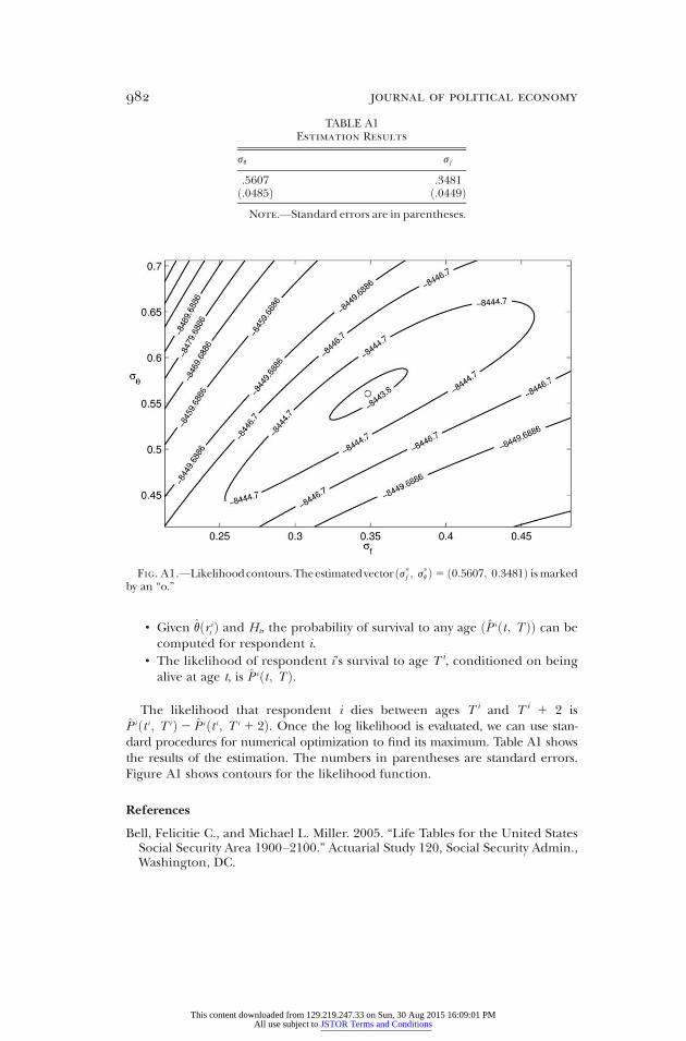
• Given vðr it Þ and Ht, the probability of survival to any age ðP iðt ; T ÞÞ can becomputed for respondent i.

TABLE A1Estimation Results

jv jf

.5607 .3481ð.0485Þ ð.0449ÞNote.—Standard errors are in parentheses.

FIG. A1.—Likelihoodcontours.Theestimatedvectorðj*f ; j*v Þ5 ð0:5607; 0:3481Þ ismarkedby an “o.”


• The likelihood of respondent i’s survival to age T i, conditioned on beingalive at age t, is P iðt ; T Þ.

The likelihood that respondent i dies between ages T i and T i 1 2 isP iðt i ; T iÞ2 P iðt i ; T i 1 2Þ. Once the log likelihood is evaluated, we can use stan-dard procedures for numerical optimization to find its maximum. Table A1 showsthe results of the estimation. The numbers in parentheses are standard errors.Figure A1 shows contours for the likelihood function.

References

Bell, Felicitie C., and Michael L. Miller. 2005. “Life Tables for the United StatesSocial Security Area 1900–2100.” Actuarial Study 120, Social Security Admin.,Washington, DC.



Benartzi, Shlomo, Alessandro Previtero, and Richard H. Thaler. 2011. “Annuiti-zation Puzzles.” J. Econ. Perspectives 25 ð4Þ: 143–64.

Bi

—

Br

Bu

Bu

Bu

C

C

D

D

Ec

Ei

Ei

Fi

—

—

Fr

G

G

H

H


sin, Alberto, and Piero Gottardi. 1999. “Competitive Equilibria with Asymmet-ric Information.” J. Econ. Theory 87 ð1Þ: 1–48.——. 2003. “Competitive Markets for Non-exclusive Contracts with AdverseSelection: The Role of Entry Fees.” Rev. Econ. Dynamics 6 ð2Þ: 313–38.own, Jeffrey R. 2001. “Private Pensions, Mortality Risk, and the Decision to An-nuitize.” J. Public Econ. 82:29–62.drıa, Santiago, Javier Dıaz-Gimenez, Vincenzo Quadrini, and Jose-Vıctor Rıos-Rull. 2011. “Facts on the Distributions of Earnings, Income and Wealth in theUnited States: 2007 Update.” Fed. Reserve Bank Minneapolis Q. Rev. 34 ð1Þ: 2–31.rman, Leonard E., Norma B. Coe, andWilliam G. Gale. 1999. “Lump SumDis-tributions from Pension Plans: Recent Evidence and Issues for Policy and Re-search.”Nat. Tax J. 52 ð3Þ: 553–62.tt, Zoltan, and Steven Haberman. 2004. “Application of Frailty-Based Mor-tality Models Using Generalized Linear Models.” Astin Bull. 34 ð1Þ: 175–97.annon, Edmund, and Ian Tonks. 2008. Annuity Markets. Oxford: Oxford Univ.Press.ristia, Julian P. 2009. “Rising Mortality and Life Expectancy Differentials byLifetime Earnings in the United States.” J. Health Econ. 28 ð5Þ: 984–95.avidoff, Thomas, Jeffrey R. Brown, and Peter Diamond. 2005. “Annuities andIndividual Welfare.” A.E.R. 95:1573–90.ubey, P., and J. Geanakoplos. 2001. “Insurance Contracts Designed by Com-petitive Pooling.” Cowles Foundation Discussion Paper no. 1315, Yale Univ.kstein, Zvi, Martin Eichenbaum, and Dan Peled. 1985. “Uncertain Lifetimesand the Welfare Enhancing Properties of Annuity Markets and Social Secu-rity.” J. Public Econ. 26 ð3Þ: 303–26.chenbaum, Martin S., and Dan Peled. 1987. “Capital Accumulation and An-nuities in an Adverse Selection Economy.” J.P.E. 95 ð2Þ: 334–54.nav, Liran, Amy Finkelstein, and Paul Shrimpf. 2010. “Optimal Mandates andthe Welfare Cost of Asymmetric Information: Evidence from the U.K. AnnuityMarket.” Econometrica 78 ð3Þ: 1031–92.nkelstein, Amy, and James Poterba. 2002. “Selection Effects in the United King-dom Individual Annuities Market.” Econ. J. 112 ð476Þ: 28–50.——. 2004. “Adverse Selection in Insurance Markets: Policyholder Evidencefrom the U.K. Annuity Market.” J.P.E. 112 ð1Þ: 183–208.——. 2006. “Testing for Adverse Selection with ‘Unused Observables.’” WorkingPaper no. 12112, NBER, Cambridge, MA.iedman, Benjamin, and Mark Warshawsky. 1990. “The Cost of Annuities: Im-plications for Saving Behavior and Bequests.” Q.J.E. 105:135–54.an, Li, Michael D. Hurd, and Daniel McFadden. 2005. “Individual SubjectiveSurvival Curves.” In Analyses in the Economics of Aging, edited by David A. Wise,377–411. Chicago: Univ. Chicago Press ðfor NBERÞ.olosov, Mikhail, and Aleh Tsyvinski. 2007. “Optimal Taxation with EndogenousInsurance Markets.” Q.J.E. 122 ð2Þ: 487–534.ansen, Gary D. 1993. “The Cyclical and Secular Behaviour of the Labour Input:Comparing Efficiency Units and Hours Worked.” J. Appl. Econometrics 8 ð1Þ: 71–80.urd, Michael D., and Kathleen McGarry. 1995. “Evaluation of the SubjectiveProbabilities of Survival in the Health and Retirement Study.” In “The Healthand Retirement Study: Data Quality and Early Results,” special issue, J. HumanResources 30:S268–S292.



———. 2002. “The Predictive Validity of Subjective Probabilities of Survival.”Econ. J. 112 ð482Þ: 966–85.


Hurd, Michael D., and Constantijn Panis. 2006. “The Choice to Cash Out Pen-sion Rights at Job Change or Retirement.” J. Public Econ. 90 ð12Þ: 2213–27.

Kotlikoff, Laurence J., and Avia Spivak. 1981. “The Family as an Incomplete An-nuities Market.” J.P.E. 89 ð2Þ: 372–91.

Krueger, Dirk, and Fabrizio Perri. 2011. “Public versus Private Risk Sharing.” J.Econ. Theory 146 ð3Þ: 920–56.

Lockwood, Lee M. 2012. “Bequest Motives and the Annuity Puzzle.” Rev. Econ.Dynamics 15 ð2Þ: 226–43.

Manton, Kenneth G., Eric Stallard, and James W. Vaupel. 1981. “Methods forComparing the Mortality Experience of Heterogeneous Populations.” Demog-raphy 18 ð3Þ: 389–410.

McCarthy, David, and Olivia S. Mitchell. 2003. “International Adverse Selectionin Life Insurance and Annuities.” Working Paper no. 9975, NBER, Cambridge,MA.

Mitchell, Olivia S., James Poterba, Mark Warshawsky, and Jeffrey Brown. 1999.“New Evidence on the Money’s Worth of Individual Annuities.” A.E.R. 89 ð5Þ:1299–1318.

Pashchenko, S. 2013. “Accounting for Non-annuitization.” J. Public Econ. 98:53–67.

Richards, Hugh, and Ronald Barry. 1998. “US Life Tables for 1990 by Sex, Race,and Education.” J. Forensic Econ. 11 ð1Þ: 9–26.

Smith, V. Kerry, Donald H. Taylor, and Frank A. Sloan. 2001. “Longevity Expecta-tions and Death: Can People Predict Their Own Demise?” A.E.R. 91 ð4Þ: 1126–34.

US Department of Labor. 1995. Retirement Benefits of American Workers: New Find-ings from the September 1994 Current Population Survey. Washington, DC: Pensionand Welfare Benefits Admin., Office Res. and Econ. Analysis.

———. 2007. “National Compensation Survey: Employee Benefits in Private In-dustry in the United States, 2005.” Bulletin no. 2589, US Dept. Labor, Washing-ton, DC.

Vaupel, James W., Kenneth G. Manton, and Eric Stallard. 1979. “The Impact ofHeterogeneity in Individual Frailty on the Dynamics of Mortality.” Demography16 ð3Þ: 439–54.

Walliser, Jan. 2000. “Adverse Selection in the Annuities Market and the Impact ofPrivatizing Social Security.” Scandinavian J. Econ. 102 ð3Þ: 373–93.



adverse selection in the annuity market and the role for

Documents