ELSEVIER Theoretical Computer Science 2 17 (1999) 235 -254

Theoretical Computer Science

Advances in the theory and practice of graph drawing’

Roberto Tamassia *

Abstract

The visualization of conceptual structures is a key component of support tools for complex

applications in science and engineering. Foremost among the visual representations used are

drawings of graphs and ordered sets. In this talk, we survey recent advances in the theory and

practice of graph drawing. Specific topics include bounds and tradeoffs for drawing properties.

tlrlce-dimensional Icpt-ebentations, methods fur constraint satisfaction, and enptlr imental studieb.

@ 1999-Elsevier Science B.V. All rights reserved

Kq~~vords: Graph drawing; 3D drawings; Constraints; Experiments

1. Introduction

In this paper, we survey selected research trends in graph drawing, and overview

some recent results of the author and his collaborators.

Graph drawing addresses the problem of constructing geometric representations of

graphs, a key component of support tools for complex applications in science and

engineering. Graph drawing is a young research field that has grown very rapidly in

the last decade. One of its distinctive characteristics is to have furthered collaborative

efforts between computer scientists, mathematicians, and applied researchers.

The book by Di Battista, et al [23] describes fundamental algorithmic techniques

graph drawing. A comprehensive bibliography on graph drawing algorithms [22] cites

more than 300 papers written before 1993. Most papers on graph drawing are cited

in yeom. bib, the computational geometry BibTEX bibliography available from

ftp:llcs. ususk. mlpuhlg~ometryl (search for keyword “graph drawing”). Surveys on var-

ious aspects of graph drawing appear in [25,34,43,46,77,7&E 1,86,89, XX, 87.841.

* Corresponding author. E-mail: rt@cs.brown.edu.

’ Research supported in part by the National Science Foundation under grants CCR-9732327 and CDA-

9703080, and by the U.S. Army Research Otfice under grant DAAH04-96-l-0013.

0304.3975/99/$-see front matter @ 1999~Elsevicr Science B.V. All rights reserved

PII: SO304-3975(98)00272-2

236 R. Tamassia I Theoretical Computer Sciencr 217 (1999) 235-254

The proceedings of the annual Symposium on Graph Drawing are published by

Springer,Verlag in the LNCS series [94,5,71,21]. Three special issues of journals

dedicated to graph drawing have been recently assembled [ 14,28,29]. Additional spe-

cial issues on selected papers from the Graph Drawing Symposia are in preparation

[26,65].

The author maintains a page (http:llwww. cs. brown. edulpeoplelrtlgd. html) with links

to graph drawing resources on the Web.

The rest of this paper is organized as follows: Section 3 overviews lower an upper

bounds on fundamental drawing properties, such as area, and gives tradeoffs between

them. Basic graph drawing terminology is reviewed in Section 2. Three-dimensional

drawings are discussed in Section 4. Section 5 deals with methods for constraint sat-

isfaction. Finally, experimental studies are reported in Section 6.

2. Graph drawing glossary

First, we define some terminology on graphs pertinent to graph drawing:

n: number of vertices of the (di)graph being considered.

m: number of edges of the (di)graph being considered.

d: maximum vertex degree (i.e., number of incident edges) of the (di)graph being

considered.

degree-k graph: graph with maximum degree d bk. digraph: directed graph, i.e., graph with directed edges (drawn as arrows).

acyclic digraph: without directed cycles.

transitive edge: edge (u,v) of a digraph is transitive if there is a directed path from u

to v not containing edge (u, v).

reduced digraph: without transitive edges.

source.. vertex of a digraph without incoming edges.

sink: vertex of a digraph without outgoing edges.

st-digraph: acyclic digraph with exactly one source and one sink, joined by an edge

(also called bipolar digraph).

connected graph: any two vertices are joined by a path.

biconnected graph: any two vertices are joined by two vertex-disjoint paths.

triconnected graph: any two vertices are joined by three vertex-disjoint paths.

tree: connected graph without cycles.

rooted tree: directed tree with a distinguished vertex, called the root, such that each

vertex lies on a directed path to the root.

binary tree: rooted tree where each vertex has at most two incoming edges.

layered (di)graph: the vertices are partitioned into sets, called layers. A rooted tree

can be viewed as a layered digraph where the layers are sets of vertices at the same

distance from the root.

k-layered (di)graph: layered (di)graph with k layers.

FIN. I. Types of drawings: (a) polyline drawing of K3.3; (b) straight-line drawing of K~,J; (c) orthogonal

drawing of IS;;; Cd) planar upward drawing of an acyclic digraph.

In a drawing of a graph, vertices are represented by points (or by geometric figures

such as circles or rectangles) and edges are represented by curves such that any two

edges intersect at most in a finite number of points. Except for Section 4, which covers

three-dimensional drawings, we consider drawings in the plane. The following types

of drawings are defined:

polylinr druv~iny: each edge is a polygonal chain (Fig. l(a)).

straight-line drming: each edge is a straight-line segment (Fig. l(b)).

orthogonal dru,c~ing: each edge is a chain of horizontal and vertical segments (Fig. 1 (c))

hmd in a polyline drawing, point where two segments part of the same edge meet

(Fig. l(a)).

cr-ossiny: point where two edges intersect (Fig. l(b)).

grid dru~~~ing: polyline drawing such that vertices, crossings and bends have integer

coordinates.

pbnur drm~img; no two edges cross (see Fig. l(d)).

pluno~ jdi)~~rupph: admits a planar drawing.

rnrhr&i& (di)gruph: planar (di)graph with a prespecified topological embedding (i.e..

set of faces), which must be preserved in the drawing.

up~u~d riruwing: drawing of a digraph where each edge is monotonically nondecreasing

in the vertical direction (see Fig. l(d)).

~lpn~rd piunur di<quph: admits an upward planar drawing.

Iu~rrrd clraGz~q: drawing of a layered graph such that vertices in the same layer arc

horizontally aligned (also called hierarchical drawing).

fticr: a region of the plane bounded by vertices and edges of a planar drawing.

c’onars drmkg: planar straight-line drawing such that the boundary of each face is a

convex polygon.

visihifit~- tlruwiny: drawing of a graph based on a geometric visibility relation. E.g.,

the vertices might be drawn as horizontal segments, and the edges associated with

vertically visible segments.

proximity drawing: drawing of a graph based on a geometric proximity relation. E.g.,

a tree is drawn as the Euclidean minimum spanning tree of a set of points.

238 R. Tumussia I Theoreticd Computer Science 217 (1999) 235-254

dominance drawing: upward drawing of an acyclic digraph such that there exists a

directed path from vertex u to vertex v if and only if x(u) <x(u) and v(u) d v(v),

where x(.) and JJ(.) denote the coordinates of a vertex.

hv-drawing: upward orthogonal straight-line drawing of a binary tree such that the

drawings of the subtrees of each node are separated by a horizontal or vertical line.

Straight-line and orthogonal drawings are special cases of polyline drawings. Poly-

line drawings provide great flexibility since they can approximate drawings with curved

edges. However, edges with more than two or three bends may be difficult to “fol-

low” for the eye. Also, a system that supports editing of polyline drawings is more

complicated than one limited to straight-line drawings. Hence, depending on the appli-

cation, polyline or straight-line drawings may be preferred. If vertices are represented

by points, orthogonal drawings exist only for graphs of maximum vertex degree 4.

3. Bounds and tradeoffs on drawing properties

For various classes of graphs and drawing types, many universal/existential upper

and lower bounds for specific drawing properties have been discovered. Such bounds

typically exhibit trade-offs between drawing properties. A universal bound applies to

all the graphs of a given class. An existential bound applies to infinitely many graphs

of the class.

Whenever we give bounds on the area or edge length, we assume that the drawing is

constrained by some resolution rule that prevents it from being arbitrarily scaled down

(e.g., requiring a grid drawing, or a minimum unit distance between any two vertices).

3.1. Bounds on the Areu

Table 1 summarizes selected universal upper bounds and existential lower bounds

on the area of drawings of graphs.

In general, the effect of bends on the area requirement is dual. On one hand, bends

occupy space and hence negatively affect the area. On the other hand, bends may help

in routing edges without using additional space.

The following comments apply to Table 1. Linear or almost-linear bounds on the

area can be achieved for trees. See Table 4 for trade-offs between area and aspect

ratio in drawings of trees. Planar graphs admit planar drawings with quadratic area.

However, the area requirement of planar straight-line drawings may be exponential if

high angular resolution is also desired. Almost linear area can be instead achieved in

nonplanar drawings of planar graphs, which have applications to VLSI circuits. Upward

planar drawings provide an interesting trade-off between area and the total number

of bends. Indeed, unless the digraph is reduced, the area can become exponential if

a straight-line drawing is required. A quadratic area bound is achieved only at the

expense of a linear number of bends.

R. Tamassial Theoretical Computer Scirnw 217 11999) 235-254 239

Table I Universal upper bounds and existential lower bounds on the area of drawings of graphs. We denote with LI

an arbitrary constant such that Oda i 1. We denote with h and (’ fixed constants such that I < h < c Class of graphs Drawing type Area Reference

Rooted tree Upward planar straight hne grid

Rooted tree Strictly upward planar straight line

Degree-O(n”) rootedtree Upward planar polyline gnd

Binaty tree Upward Planar orthogonal gnd

Tree Planar straight line grid

Degree-O( na ) tree Planar polyline grid

Degree-4 tree Planar orthogonal grid

Planar graph Planar polyline grid

Planar graph Planar straight line

Planar graph Planar straight line grid

l‘ruxmected planar graph Planar straight line convex grid

Planar graph Planar orthogonal grid

Planar degree-4 graph Orthogonal grid

Upward planar dlgraph Upward planar gnd straight lnx

Reduced planar sf-dlgraph Upward planar grid stmght line

Upward planar digraph

General graph

dominance

Upward planar grid polyline

Polylmr grid

O( n log II )

0(/I log /I)

0t II ) O(n log log n O(n log n) O(,I) an)

01!?)

od ) 7 ocn- ) Od) O(n log? n)

<1(<“)

O(r? ) [.30]

!)(I? ) 12:. 301

O((n + %)‘I

Table 2

Universal lower bounds and existential upper bounds on the angular resolution of drawings of graphs WC

denote with c a fixed constant such that c > I Class of graphs Drawing type Angular resolution Refcrcnce

General graph Straight line !I( 1/d2) O(log did*) [371 Planar graph

Planar graph

Straight line

Planar straight line

<2(1/d)

!I( I /cd ) 0( I/d)

o(&zq [371

[42. 6X I

3.2. Bow& on the Anyukur Resolution

Table 2 summarizes selected universal lower bounds and existential upper bounds

on the angular resolution of drawings of graphs.

3.3. B0und.y on the number of Bends

Table 3 summarizes selected universal upper bounds and existential lower bounds

on the total and maximum number of bends in orthogonal drawings. Some bounds are

stated for n 3 5 or > 7 because the maximum number of bends is at least 2 for KJ and

at least 3 for the skeleton graph of an octahedron, in any planar orthogonal drawing.

3.4. Tradewf between urea and aspect-ratio

The ability to construct area-efficient drawings is essential in practical visualization

applications, where screen space is at a premium. However, achieving small area is

not enough: e.g., it is easy to see that a drawing with high aspect ratio may not be

conveniently placed on a workstation screen, even if it has modest area. Hence, it is

important to keep the aspect ratio small. Ideally, one would like to obtain small area

240 R. Tamassia / Theoretical Computer Science 217 (1999) 235-254

Table 3

Orthogonal drawings: universal upper bounds and existential lower bounds on the total and maximum number

of bends

Class of graphs Drawing type Total no. bends Max no. bends Reference

Degree-4 grapha Orthogonal >n 62n+2 >2 $2 [3] Planar degree-4 grapha Orthogonal planar >2n - 2 <2n+2 >2 <2 [3, 951

Embedded degree-4 graph Orthogonal planar a2n - 2 Gyni2 23 <3 [36,67,92,95] Biconnected embedded degree-4 graph Orthogonal planar >2n - 2 <2n+2 >,3 <3 [36,67,92, 951

Triconnected embedded degree-4 graph

Embedded degree-3 graphb

Orthogonal planar >$(n- 1)+2 <in+4 32 $2 [59]

Orthogonal planar > in + 1 -sin+1 21 <l [59,66]

Table 4

Universal upper bounds that can be simultaneously achieved for the area and aspect-ratio in drawings of

trees. We denote with a an arbitrary constant such that O<a < 1

Class of graphs Drawing type Area Aspect-Ratio Reference

Rooted tree Upward planar straight line

layered grid 0(n2) O(1) [751 Rooted tree Upward planar straight line grid O(n log n) O(n 1 log n) [12,821 Rooted degree-0( 1) tree Upward planar polyline grid O(n) O(n” ) [401

Binary tree Upward planar orthogonal grid O(n log log n) O(n log log n/ log2 n) [401 Degree-4 tree Orthogonal grid O(n) O(1) [99,621 Degree-4 tree Orthogonal grid, leave

on convex hull O(n log n) O(1) 171

for any given aspect ratio in a wide range. This would provide graphical user interfaces

with the flexibility of fitting drawings in arbitrarily shaped windows.

A variety of trade-offs for the area and aspect-ratio arise even when drawing graphs

with a simple structure, such as trees. Table 4 summarizes selected universal bounds

that can be simultaneously achieved on the area and the aspect ratio of various types

of drawings of trees.

While upward planar straight line drawings are the most natural way of visualizing

rooted trees, the existing drawing techniques are unsatisfactory with respect to either the

area requirement or the aspect ratio. The situation is similar for orthogonal drawings.

Regarding polyline drawings, linear area can be achieved with a prescribed aspect

ratio [40]. However, experiments show that this is done at the expense of a somehow

aesthetically unappealing drawing.

For non-upward drawings of trees, linear area and optimal aspect ratio are possible

for planar orthogonal drawings, and a small (logarithmic) amount of extra area is

needed if the leaves are constrained to be on the convex hull of the drawing (e.g.,

pins on the boundary of a VLSI circuit). However, the non-upward drawing methods

do not seem to yield aesthetically pleasing drawings, and are suited more for VLSI

layout than for visualization applications.

3.5. Trade-of between area and angular resolution

Table 5 summarizes selected universal bounds that can be simultaneously achieved

on the area and the angular resolution of drawings of graphs.

R. Tunzussiu I Theoretical Computtv- Scirnw 217 i 1999) 235~.254 241

Table 5

Universal asymptotic upper bounds for the area and lower bounds for the angular resolution that can bc

simultaneously achieved in drawings of graphs. We denote wtth h and c fixed constants such that h ‘> I and c’ > I

Class of graphs Drawing type .Area Angular resolution Rcferencc

Planar graph Straight line O(d’n) (I( l/d?) P71 Planar graph Straight line O(d’n) <I( I,“d) 1371 Planar graph Planar straightline grid O(n’ ) !I( l/r?) [ 19. X0]

Planar graph Planar straight line O(F) Q( I/Jcd) [6X1 Planar graph Planar polyline grid O(n’) n(ljd) [591

Universal lower bounds on the angular resolution exist that depend only on the

degree of the graph. Also, substantially better bounds can be achieved by drawing a

planar graph with bends or in a non-planar way.

3.6. Open probkms

Determine the area requirement of (upward) planar straight-line drawings of trees.

There is currently an O(log n) gap between the known upper and lower bounds

(Table 1).

Determine the area requirement of orthogonal (or, more generally, polyline) non-

planar drawings of planar graphs. There is currently an O(log n) gap between the

known upper and lower bounds (Table 1).

Close the gap between the 12( l/d2) universal lower bound and the O(log d/d’ )

existential upper bound on the angular resolution of straight-line drawings of general

graphs (Table 2).

Close the gap between the 62( l/cd) universal lower bound and the 0( dw)

existential upper bound on the angular resolution of planar straight-line drawings of

planar graphs (Table 2).

Determine the best-possible aspect ratio and area that can be simultaneously achieved

for (upward) planar straight-line and orthogonal drawings of trees (Table 4).

4. Three-dimensional drawings of graphs

Recent advances in hardware and software technology for computer graphics open the

possibility of displaying three-dimensional (3D) visualizations on a variety of low-cost

workstations, and a handful of researchers (and film makers 2 ) have begun to explore

the possibilities of displaying graphs using this new technology. Previous research

on 3D graph drawing has focused on the development of visualization systems (see,

e.g. [76,79]). Much work needs to be done on the theoretical foundations of 3D graph

drawing. Recent progress has been reported in [8,9,35,45,53,64].

* An important plot element in the movie Jurussic Purk involves a 3D virtual-reality traversal of a tree

representing a Unix file system.

242 R. Tumussiu I Theoretical Computer Science 217 (1999) 235-254

Fig. 2. Example of a 3D convex drawing.

4.1. 30 convex drawings

A 3D convex drawing of a graph G is a realization of G by the skeleton of a 3D

convex polytope (see Fig. 2. The well-known Steinitz’s theorem says that a graph ad-

mits a 3D convex drawing if and only if it is planar and triconnected [83] (see also

[44]), properties that can be verified in linear time (see, e.g. [50,51]). Interestingly,

it is a simple exercise to derive from the published proofs of Steinitz’s theorem a

cubic-time method for constructing 3D convex drawings in the real-RAM model [74].

Unfortunately, this approach seems to require at least exponential volume and an ex-

ponential number of bits to implement. Indeed, Onn and Sturmfels [72] show how to

construct a 3D convex grid drawing within a cube of side O(PZ’~~~‘).

Maxwell [70] (see also [ 10, 11, loo]) describes a mapping that transforms a 2D con-

vex drawings with a certain “equilibrium stress property” into a 3D convex drawing.

Further results on this transformation are given by Hopcroft and Kahn [52]. Eades

and Garvan [33] show how to construct 3D convex drawings by combining the above

transformation with the 2D-drawing method of Tutte [97,98]. They also show that

their drawings have exponential volume in the worst case. Smith (see [49]) claims a

polynomial-time algorithm for constructing a 3D convex drawing inscribed in a sphere,

with vertex coordinates represented by O(n log n)-bit numbers, for an n-vertex graph

known to be inscribable (which can be tested in linear time, e.g., for planar triangula-

tions, due to a result of Dillencourt and Smith [32]). Das and Goodrich [17] present a

linear-time algorithm for constructing a 3D convex drawing of a maximal planar graph

such that the vertex coordinates are rational numbers that can be represented with a

polynomial number of bits.

Chrobak et al. [8] have recently shown how to construct in O(H’.~) time a 3D

convex drawing with O(n) volume such that the vertex coordinates are represented by

O(n log tr)-bit rational numbers and any two vertices are at distance at least one.

5. Constraint satisfaction in graph drawing

Research in graph drawing has traditionally focused on algorithmic methods, where

the drawing of the graph is generated according to a prespecified set of aesthetic

criteria (such as planarity or area minimization) that are embodied in an algorithm.

Although the algorithmic approach is computationally efficient, it does not naturally

support constraints, i.e., requirements that the user may want to impose on the drawing

of a specific graph (e.g., clustering or aligning a given set of vertices). Previous work

has shown that only a rather limited constraint satisfaction capability can be added to

existing drawing algorithms (see, e.g.[3 1,901).

Recently, several attempts have been made at developing languages for the specifica-

tion of constraints and at devising techniques for graph drawing based on the resolution

of systems of constraints (see, e.g. [20,57,69]). Eades and Lin [63] attempt at com-

bining algorithmic and declarative methods in drawings of trees. Brandenburg presents

a comprehensive approach to graph drawing based on graph grammars [4].

5.1. Visuul gruph rlraw+zy

A visual approach to graph drawing, where the layout of a graph is pictorially speci-

fied “by example”, is proposed by Cruz et al [ 15, 161. Within this approach, a graph is

stored in an object-oriented database, and its drawing is defined used recursive visual

rules of the visual meta-language DOODLE [13]. The following types of drawings

can be visually expressed in such a way that the system of constraints obtained from

the application of the visual rules to the input graph can be solved in linear time:

l level drawings and box inclusion drawings of binary trees;

l a-drawings of series-parallel digraphs [I];

l polyline drawings (271, visibility drawings [91], and tessellation drawings [93] of

upward planar digraphs (see Fig. 3).

In the rest of this section, we present visual programs for drawing a planar st-

digraph, i.e., an embedded planar acyclic digraph with exactly one source and one

sink, joined by an edge. Such digraphs play an important role in the theory of ordered

sets since their transitive reductions are the covering digraphs of planar lattices [61].

Such visual programs can be easily modified to construct drawings of upward planar

digraphs, which are known to be subgraphs of planar st-digraphs [60,27].

244 R. Tumassiu I Theoretical Computer Science 217 (1999) 235-254

Fig. 3. Drawings of a planar st-digraph: (a) tessellation drawing; (b) visibility drawing; (c) upward polyline

drawing.

We show in Fig. 4 a complete visual program for tessellation representations. We

assume that the vertices, edges, and faces of the input planar st-digraph G are database

objects, where for each object o the following attributes describing the embedding are

stored: left face l@(o), right face right(o), bottom vertex hot(o), and top vertex top(o).

note that the value of each attribute is another database object.

Each rule defines the visual representation of a database object of a certain class

(vertex, edge, and face). For tessellation representations, this is a horizontal segment

for a vertex, a vertical segment for a face, and a rectangle for an edge. The visual

notation in the rule for an object o includes:

geometric figures that give the visual representation of object o, such as circles,

segments, and rectangles;

references to the visual representation of other objects given by attributes of o,

denoted with dashed boxes labeled by the attribute;

landmarks of the visual representations of o and of other referenced objects, shown

as small squares with labels (e.g., MS, the “middle South” landmark, denotes the

middle point of the bottom edge of a rectangle); and

landmarks of the coordinate system, shown with small circles (e.g., ORIGIN denotes

point (0,O));

explicit constraints between landmarks, shown as arrows joining two landmarks with

labels defining the constraint imposed on the coordinates of the landmarks (e.g.,

in rule (d), the dashed arrow with label max(l,A)[h,v] is an explicit constraint

R. Tumassia I Theoretical Computer Science 217 (1999) 235-254

TessellationDrawing

f: ‘face . . . . . . . . . . . . . . . . . . : top(f)

Tassallationkawing

245

I 1 TessellationDrawing I e:edge

Fig. 4. Visual rules for constucting a tessellation drawing of a planar st-digraph:

special rule for the source vertex; (c) rule for a vertex; (d) rule for an edge.

‘a) rule for a face; (b)

.

specifying minimum horizontal and vertical distance 1 from the “midpoint South”

MS to the “midpoint East” of the rectangle);

implicit constraints between landmarks, given by their horizontal or vertical align-

ment (e.g., in rule (d), the “midpoint East” ME of the rectangle representing edge

e and the “top endpoint” TE of the referenced visual representation of the right

face of eright(e) must have the same x-coordinate because they are drawn vertically

aligned).

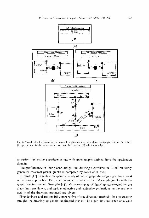
Complete visual programs for visibility representations and upward polyline drawings

are shown in Fig. 5 and 6, respectively. In these two programs, the visual representation

of the faces is a single point associated with landmark F. This point is invisible but

contributes to the definition of the constraints. Also, the visual representation of an

edge includes a visible portion (vertical segment for a visibility representation and

246 R. Tumussiu I Theoretical Computer Science 217 (1999) 235-254

1 VisibilityDrawing 1

f: face

VisibilityDrawing

v: sourceVe&x

ORIGIN . . . . . . . . .

. . . . . . : . F?* 0,5 [i-l] i left(v); ‘+ i m-a* i ; . . LE RE . . . . . . . . :nght(v):

I ;I . . . . . . . . .

(b) Cc)

VisibilityDrawing

e:edge

(4

Fig. 5. Visual roles for constucting a visibility representation of a planar sr-digraph: (a) role for a face; (b)

special rule for the source vertex; (c) rule for a vertex; (d) rule for an edge.

polygonal chain with three segments for an upward polyline drawing) and an invisible

portion drawn with a conventional “transparent color” (a rectangle or segment with

shaded lines in the figures).

6. Experimental graph drawing

Many graph drawing algorithms have been implemented and used in practical appli-

cations. Most papers show sample outputs, and some also provide limited experimental

results on small test suites (see, e.g. [l&38,39,55,57,58] and the experimental pa-

pers in the Graph Drawing Symposia). However, in order to evaluate the practical

performance of a graph drawing algorithm in visualization applications, it is essential

R. Tumassia I Theorericul Computer Scirnw 217 ( 1999 I 235-254 247

1 PolyllneDrawing [

f: face

PolylineDrawing

v: sourceVertex v: vertex

. . . . . . . . .

i left(v)

: right(v)! . . . . . . . . . . . . .

(b) (cl Poly1ineDrawin-J

e:edge

Cd)

Fig. 6. Visual rules for constucting an upward polyline drawing of a planar .st-digraph: (a) rule for a face;

(b) special rule for the source vertex; (c) rule for a vertex; (d) rule for an edge.

to perform extensive experimentations with input graphs derived from the application

domain.

The performance of four planar straight-line drawing algorithms on 10 000 randomly

generated maximal planar graphs is compared by Jones et al. [54].

Himsolt [47] presents a comparative study of twelve graph drawings algorithms based

on various approaches. The experiments are conducted on 100 sample graphs with the

graph drawing system GmphEd [48]. Many examples of drawings constructed by the

algorithms are shown, and various objective and subjective evaluations on the aesthetic

quality of the drawings produced are given.

Brandenburg and Rohrer [6] compare five “force-directed” methods for constructing

straight-line drawings of general undirected graphs. The algorithms are tested on a wide

248 R. Tumussial Theoreticul Computer Science 217 (1999) 235-254

collection of examples and with different settings of the force parameters. The quality

measures evaluated are crossings, edge length, vertex distribution, and running time.

They also identify trade-offs between the running time and the aesthetic quality of the

drawings produced.

Jiinger and Mutzel [56] investigate crossing minimization strategies for straight-line

drawings of 24ayer graphs, and compare the performance of eight popular heuristics

for this problem.

6.1. Ezcperiments on orthogonal drawings

In [24] Di Battista et al. present an extensive experimental study comparing four

general-purpose graph drawing algorithms. The four algorithms, denoted Bend-Stretch,

Column, Giotto, and Pair, take as input general graphs (with no restrictions whatsoever

on the connectivity, planarity, etc.) and construct orthogonal grid drawings, which are

widely used in software and database visualization applications.

Algorithms Bend-Stretch and Giotto are based on a general approach where the

drawing is incrementally specified in three phases: The first phase, planarization, de-

termines the topology of the drawing. The second phase, orthogonalization, computes

an orthogonal shape for the drawing. The third phase, compaction, produces the final

drawing. This approach allows homogeneous treatment of a wide range of diagram-

matic representations, aesthetics and constraints (see, e.g., [58,90,96]) and has been

successfully used in industrial tools. The main difference between the two algorithms

is in the orthogonalization phase: Algorithm Giotto uses a network-flow method that

guarantees the minimum number of bends but has quadratic time complexity [85]. Al-

gorithm Bend-Stretch adopts the “bend-stretching” heuristic [92] that only guarantees

a constant number of bends on each edge but runs in linear time.

Algorithm Column is an extension of the orthogonal drawing algorithm by Biedl and

Kant [3] to graphs of arbitrary vertex degree. The orthogonal grid drawing is incremen-

tally constructed by adding the vertices one at a time. Namely, at each step a vertex v

is added plus the edges connecting v to previously added vertices. Some columns of the

grid are “reserved” to draw the remaining incident edges of v. Concerning the position

of v, since one row is used for each vertex, the y-coordinate is immediately given by

the order of visit of v, and the x-coordinate is the one of the reserved column of the

incident edge of v that minimizes the number of bends introduced by the new edges.

Algorithm Pair is an extension of the orthogonal drawing algorithm by Papakostas and

Tollis [73] to graphs of arbitrary vertex degree.

Examples of “typical” drawings generated by Bend-Stretch, Column, Giotto, and

Pair are shown in Fig. 7.

The test data (available on the Internet) are 11,582 graphs, ranging from 10 to

100 vertices, generated from a core set of 112 graphs used in “real-life” software

engineering and database applications. The experiments provide a detailed quantitative

evaluation of the performance of the four algorithms and show that they exhibit trade-

offs between “aesthetic” properties (e.g., crossings, bends, edge length) and running

R. Tamassia I Theoretical Computer Science 217 (1999) 235-254 249

p_- L.

- (b)

F r _ -

- - - -

t_

P‘

- - - - -

f

- Q %

(4

Fig. 7. Drawings of the same 63-vertex graph produced by algorithms (a) Bend-Stretch, (b) Giotto, (c)

Column, and (d) Pair, respectively.

250 R. Tamassia I Theoretical Computer Science 217 (1999) 235-254

(4

(b)

Fig. 8. (a) Average area versus number of vertices. (b) Average number of crossings versus number of

vertices. (c) Average CPU time (seconds) versus number of vertices.

time. For example, Fig. 8 shows the average area number of crossings, and CPU time.

The observed practical behavior of the algorithms is consistent with their theoretical

properties. Namely, Giotto outperforms the other algorithms for most quality measures

but is considerably slower than Column and Pair.

References

[I] P. Bertolazzi, R.F. Cohen, G. Di Battista, R. Tamassia, LG. Tollis. How to draw a series-parallel

digraph, Internat. J. Comput. Geom. Appl. 4 (1994) 385402.

R. Tomussiu I Theoretical Computer Scienw 217 ilY99) 235-254 251

[Z] S.N. Bhatt, F.T. Leighton, A framework for solving VLSI graph layout problems. J. Comput. Systems.

Sci. 28 (1984) 300-343.

[3] T. Biedl. G. Kant, A better heuristic for orthogonal graph drawings. Comput. Geom. Theory Appl. 9

(1998) 159~180.

[4] F.J. Brandenburg, Designing graph drawings by layout graph grammars, in: R. Tamassia. I.G. 7‘0111s

(Eds), Graph Drawing (Proc. GD ‘94), Lecture Notes Comput. Sci., vol. X94. Springer. Berlin. 1995.

pp. 416427.

[S] F.J. Brandenburg (Ed.) Graph Drawing (Proc. GD ‘95) Lecture Notes Comput. Sci., vol. 1027. Springer.

Berlin, 1996.

[6] F.J. Brandenburg, M. Himsolt, C. Rohrer, An experimental comparison of force-directed and randomized

graph drawing algorithms, in: F.J. Brandenburg(Ed.), Graph Drawing (Proc. GD ‘95) Lecture Notes

Comput. Sci., vol. 1027 Springer, Berlin, 1996, pp. 76687.

[7] R.P. Brent, H.T. Kung. On the area of binary tree layouts. Inform. Process. Lett. I I (1980) 521-534.

[X] M. Chrobak, M.T. Goodrich, R. Tamassia. Convex drawings of graphs in two and three dimensions.

Proc. 12th Ann. ACM Symp. Comput. Geom., 1996, pp. 319328.

[9] R.F. Cohen. P. Eades, T. Lin, F. Ruskey. Three-dnnensional graph drawing. in: R. Tamassra, I.G. ToIlls

(Eds.), Graph Drawing (Proc. GD ‘94). Lecture Notes Comput. SCI.. vol. X94, Springer, Berlin. 1995.

pp. l-1 I.

[IO] R. Connelly. Rigidity and energy, Invent. Math. 66 (1982) I l-33.

[I I] H. Crapo, W. Whitely, Statics of frameworks and motions of panel structures. a projective geometric

introduction, Struct. Topol. 6 (1982) 42-82.

[ 121 P. Crescenzi. G. Di Battista, A. Pipemo, A note on optimal area algorithms for upward drawmgs of

binary trees. Comput. Geom. Theory Appl. 2 (I 992) 187-200.

[ 131 I.F. Crux. DOODLE: a visual language for object-oriented databases, Proc. ACM SIGMOD Conf. on

Management of Data, 1992, pp. 71-80.

[ 141 I.F. Crux, P. Eadcs (Eds.) Special Issue on Graph Visualization, J. Visual Lang. Comput. 6 (3) 1995.

[ 151 I.F. Crux. A. Garg, Drawing graphs by example efficiently: trees and planar acyclic digraphs, m:

R. Tamassia. I.G. Tollis (Eds.) Graph Drawing (Proc. GD ‘94). Lecture Notes Comput. Sci., vol.

894, Springer. Berlin, 1995, pp. 404415.

[ Ih] I.F. Crur, A. Garg. R. Tamassia. Efficient constraint resolution in visual graph drawing. Manuscript.

Dept. of Computer Sci., Brown University. 1996.

[ 171 G Das, M.T. Goodrich. On the complexity of optimization problems for 3-dimensional convex polyhedra

and decision trees, Comput. Geom. Theory Appl. 8 (1997) 123-l 37.

[IR] R. Davidson, D. Harel, Drawing graphics nicely using simulated annealing. ACM Trans. Graph. l5(4)

(1996) 301-331.

[I91 H de Fraysseix. J. Path, R. Pollack, How to draw a planar graph on a gnd, Combinatorics, lO( I ) (1990) 41-51.

[20] E. Dengler. M. Friedell, J. Marks, Constraint-driven diagram layout. Proc. IEEE Symp. on Visual

Languages 1993, pp. 330-335.

[2l] G. Di Battista (Ed.), Graph Drawing (Proc. GD ‘97). Lecture Notes Comput. Sci., vol. 1353, Springer.

Berlin, 199X.

[22] G. Di Battista, P. Eades, R. Tamassia, LG. Tollis, Algorithms for drawing graphs: an annotated

bibliography, Comput. Geom. Theory Appl. 4 ( 1994) 235-282.

[23] G. Di Battista, P. Eades, R. Tamassia, I.G. ‘Tollis, Graph Drawing. Prentice-Hall. Englewood Clih’s. NJ.

1098.

[24] G. Di Battista, A. Garg, G. Liotta, R. Tamassia, E. Tassinari, F. Vargru, An experimental comparison

of four graph drawing algorithms, Comput. Geom. Theory Appl. 7 (1997) 303-325.

[25] G. Di Battista. W. Lenhart, G. Liotta, Proximity drawability: a survey, In: R. Tamassia, I. G. Tollis

(Eds.). Graph Drawing (Proc. GD ‘94), Lecture Notes Comput. Sci.. vol. 894 Springer. Berlin. 1995.

pp. 328-339.

[26] G. Di Battista, P. Mutzel (Eds.), Special Issue on Selected Papers from the 1997 Symposium on Graph

Drawing, J. Graph Algorithms Appl., to appear.

[27] G. Di Battista, R. Tamassia, Algorithms for plane representations of acychc digraphs, Theoret. Comput.

Sci. 61 (1988) 175-198.

[2X] G. Di Battista, R. Tamassia (Eds.) Special Issue on Graph Drawing. Algorithmica, vol. l6( I ) ( 1996).

252 R. Tumussial Theoretical Computer Science 217 (1999) 235-254

[29] G. Di Battista, R. Tamassia (Eds.) Special Issue on Geometric Representations of Graphs, Comput.

Geom. Theory Appl. vol. 9( 1-2) (1998). [30] G. Di Battista, R. Tamassia, I. G. Tollis, Area requirement and symmetry display of planar upward

drawings, Discrete Comput. Geom. 7 (1992) 381401.

[31] G. Di Battista, R. Tamassia, I.G. Tollis, Constrained visibility representations of graphs, Inform. Process.

Lett. 41 (1992) 1-7.

[32] M. B. Dillencourt, W.D. Smith, A linear-time algorithm for testing the inscribability of trivalent

polyhedra, Internat. J. Comput. Geom. Appl. 5 (1995) 21-36.

[33] P. Eades, P. Garvan, Drawing stressed planar graphs in three dimensions, F. J. Brandenburg (Ed.) Graph

Drawing (Proc. GD ‘95), Lecture Notes Comput. Sci., vol. 1027, Springer, Berlin, 1996.

[34] P. Eades, X. Lin, How to draw a directed graph, Proc. IEEE Workshop on Visual Languages, 1989,

pp. 13-17. [35] P. Eades, C. Stirk, S. Whitesides, The techniques of Kolmogorov and Bardzin for three dimensional

orthogonal graph drawings, Inform. Process. Lett. 60 (1996) 97-103.

[36] S. Even, G. Granot, Rectilinear planar drawings with few bends in each edge. Technical Report 797,

Computer Science Dept., Technion, 1994.

[37] M. Formann, T. Hagerup, J. Haralambides, M. Kaufmann, F.T. Leighton, A. Simvonis, E. Welzl,

G. Woeginger, Drawing graphs in the plane with high resolution, SIAM J. Comput. 22 (1993) 1035%

1052. [38] T. Fruchterman, E. Reingold, Graph drawing by force-directed placement, Software ~ Pratt. Exp. 2 I(1 1)

(1991) 1129-1164.

[39] E.R. Gansner, S.C. North, K.P. Vo, DAG ~ A program that draws directed graphs, Software ~ Pratt.

Exp. 18(11) (1988) 1047-1062.

[40] A. Garg, M. T. Goodrich, R. Tamassia, Planar upward tree drawings with optimal area, lntemat. J.

Comput. Geom. Appl. 6 (1996) 333-356. [41] A. Garg, R. Tamassia, Efficient computation of planar straight-line upward drawings, Graph Drawing

‘93, Proc. ALCOM Workshop on Graph Drawing, 1993.

[42] A. Garg, R. Tamassia, Planar drawings and angular resolution: algorithms and bounds, Proc. 2nd Ann.

Eur. Symp. Algorithms, Lecture Notes Comput. Sci., vol. 855, Springer, Berlin, 1994 pp. 12-23.

[43] A. Garg, R. Tamassia, Upward planarity testing, Order 12 (1995) 1099133.

[44] B. Griinbaum, Convex Polytopes, Wiley, New York, NY, 1967.

[45] SM. Hashemi, I. Rival, Upward drawings to fit surfaces, Proc. Workshop on Orders, Algorithms and

Applications, Lecture Notes Comput. Sci., vol. 831, Springer, Berlin, 1994, pp. 53-58. [46] X. He, M.-Y. Kao, Regular edge labelings and drawings of planar graphs, R. Tamassia, 1. G. Tollis

(Eds.) Graph Drawing (Proc. GD ‘94) Lecture Notes Comput. Sci., vol. 894, Springer, Berlin, 1995.

pp. 96103.

[47] M. Himsolt, Comparing and evaluating layout algorithms within GraphEd, J. Visual Lang. Comput.

6(3) (1995) 255-273. (special issue on Graph Visualization, edited by 1. F. Cruz, P. Eades).

[48] M. Himsolt, GraphEd: a graphical platform for the implementation of graph algorithms, in: R. Tamassia,

I.G. Tollis (Eds.), Graph Drawing (Proc. GD ‘94), Lecture Notes Comput. Sci., vol. 894, Springer,

Berlin, 1995, pp. 1822193. [49] C.D. Hodgson, I. Rivin, W.D. Smith, A characterization of convex hyperbolic polyhedra and of convex

polyhedra inscribed in the sphere, Bull. (New Series) Amer. Maths. Sot. 27(2) (1992) 246-251.

[50] J. Hopcroft, R.E. Tarjan, Dividing a graph into triconnected components, SIAM J. Comput. 2(3) (1973)

135-158.

[51] J. Hopcroft, R.E. Tarjan, Efficient planarity testing, J. ACM 21(4) (1974) 549-568. [52] J.E. Hopcroft, P.J. Kahn, A paradigm for robust geometric algorithms, Algorithmica 7(4) (1992) 339-

380. [53] T. J&on, C. Jard, 3D layout of reachability graphs of communicating processes, in: R. Tamassia, I. G.

Tollis (Eds.), Graph Drawing (Proc. GD ‘94), Lecture Notes Comput. Sci., vol. 894, Springer, Berlin,

1995, pp. 25-32. [54] S. Jones, P. Eades, A. Moran, N. Ward, G. Delott, R. Tamassia, A note on planar graph drawing

algorithms, Technical Report 216, Department of Computer Science, University of Queensland, 1991,

[55] M. Jiinger, P. Mutzel, Maximum planar subgraphs and nice embeddings: practical layout tools,

Algorithmica l6( I ) (1996) 33-59. (special issue on Graph Drawing, edited by G. Di Battista, R.

Tamassia).

R. Tumussia I Theoreticul Computer S&we 217 i 19991 235%2.~4 253

[56] M. Jiinger, P. Mutzel, 2-Layer straightline crossing minimization: performance of exact and heuristic

algorithms, J. Graph Algorithms Appl. l(1) (1997) l-25.

[57] T. Kamada, Visualizing Abstract Objects and Relations, World Scientific Series in Computer Sclencc.

Singapore. 1989.

[5X] G. Kant, Algorithms for drawing planar graphs. Ph.D. Thesis, Dept. Comput. SCI., Univ. Utrecht. Utrccht.

Netherlands, 1993.

[59] G. Kant, Drawing planar graphs using the canonical ordering, Algorithmica 16 (1996) 4-32. (special

issue on Graph Drawing, edited by G. Di Battista. R. Tamassia).

[60] D. Kelly, Fundamentals of planar ordered sets, Diccrete Math. 63 (1987) 197-216.

[61] D. Kelly, I. Rival, Planar lattices, Canad. J. Math. 27(3) (1975) 636-665.

[62] C.E. Leiserson, Area-eficient graph layouts (for VLSI). Proc. 2lst Ann. IEEE Symp. Found. Comput.

Sci., 1980 pp. 270-281.

[63] T. Lin. P. Eades. Integration of declarative and algorithmic approaches for layout creation. III:

R. Tamassia. I.G. Tollis (Eds.). Graph Drawing (Proc. GD ‘94). Lecture Notes Comput. Sci.. vol.

894, Springer. Berlin, 1995, pp. 376-387.

[64] G. Liotta, G. Di Battista, Computing proximity drawings of trees in the 3-dimensional space. Proc. 4th

Workshop Algorithms Data Struct.. Lecture Notes Comput. Sci.. vol. 955. Springer, Berlin. 1995. pp.

239-250.

[65] G. Liotta, S. Whitesides (Eds.) Special Issue on Selected Papers from the 1998 Symp. on Graph

Drawing. J. Graph Algorithms Appl., to appear.

1661 Y. Liu. P. Marchioro, R. Petreschi, B. Simeone, Theoretical results on at most l-bend embeddability

of graphs, Technical report, Dipartimento di Statistica, Univ. di Roma “La Sapienra“. IY90.

[67] Y. Liu, A. Morgana, B. Simeone, General theoretical results on rectilinear embeddability of graphs,

Acta Math. Appl. Sinica 7 (1991) 1X7-192.

[6X] S. Malit/. A. Papakostas. On the angular resolution of planar graphs. SIAM J. Discrete Math. 7 ( 1904)

172-183.

(691 J. Marks, A formal specification for network diagrams that facilitates automated design, J. Visual Lang.

Comput. 2 (1991) 395-414.

1701 J.C. Maxwell, On reciprocal figures and diagrams of forces, Philos. Mag. Ser. 27 (I X64) 250-261.

1711 S.C. North (Ed.) Graph Drawing (Proc. GD ‘96). Lecture Notes Comput. Sci.. vol. 1100. Springer.

Berlin, 1997.

[72] S. Onn. B. Sturmfels, A quantitative Steinitz’ theorem. Beitrage zur Algebra und Geometric,

Contributions to Algebra and Geometry 35 (1994) 125%12Y.

[73] A. Papakostas. I.G. Tollis. Algorithms for arca-efficient orthogonal drawings. Comput. Gcom. Theory

Appl. 9( l-2) (1998) 83-l IO.

[74] F. P. Preparata, M. I. Shamos, Computational Geometry: An Introduction, Sponger. Berlin. New York.

NY, 1985.

[75] E. Reingold, J. Tilford, Tidier drawing of trees. IEEE Trans. Software. Eng. SE-7(2) (19X1 ) 223-228.

[76] S. P. Reiss, An engine for the 3D visualization of program information, J. Visual Lang. Comput. h( 3)

(1995) 299-323. (special issue on Graph Visualization, edited by I.F. Cruz, P. Eades).

[77] I. Rival, Graphical data structures for ordered sets, in: I. Rival (Ed.). Algorithms and Order. Kluwer

Academic Publishers, Dordrecht, 19X9 pp. 3-3 I [7X] 1. Rival. Reading. drawing, and order, in: 1. G. Rosenberg, G. Sabidussi (Eds.), Algebras and Orders,

Kluwcr Academic Publishers, Dordrecht, 1993 pp. 359404.

[79] G.G. Robertson, J.D. Mackinlay, S.K. Card. Cone trees: animated 3D visualizations of hierarchical

information. Proc. ACM Conf. on Human Factors in Computing Systems. 199 I. pp. I X9-l 93.

[X0] U’. Schnyder. Embedding planar graphs on the grid, Proc. 1st ACM-SIAM Symp. Discrete Algorithm>. lY90 pp.l38-148.

[Xl] F. Shahrokhi. L. A. Szt-kely. I. Vrt’o, Crossing numbers of graphs. lower bound techniques and

algorithms: a survey, in: R. Tamassia,l. G. Tollis (Eds.) Graph Drawing (Proc. GD ‘94). Lecture Notes C‘omput. Sci., vol. X94, Springer, Berlin, 1995, pp. 131-142.

[X2] Y. Shiloach, Arrangements of Planar Graphs on the Planar Lattice, Ph.D. Thesis, Weizmann Institute

of Science. 1976.

[X3] E. Stelnitr. H. Rademacher, Vorlesungen fiber die Theorie dcr Polyedcr. Julius Springer, Hcrlin.

Germany. 1934.

254 R. Tamassial Theoreticd Computer Science 217 (1999) 235-254

[84] R. Tamassia, Graph drawing, in: J.-R. Sack, J. Urrutia (Eds.), Handbook of Computational Geometry,

Elsevier Science Publishers B.V., North-Holland, Amsterdam, 1998, to appear.

[85] R. Tamassia, On embedding a graph in the grid with the minimum number of bends, SIAM J. Comput.

16(3) (1987) 421444.

[86] R. Tamassia, Drawing algorithms for planar St-graphs, Aust. J. Combin. 2 (1990) 217-235.

[87] R. Tamassia, Planar orthogonal drawings of graphs, Proc. IEEE Internat. Symp. on Circuits Systems,

1990.

[88] R. Tamassia, Graph drawing, in: J.E. Goodman, J. O’Rourke (Eds.), Handbook of Discrete and

Computational Geometry, ch. 44, CRC Press LLC, Boca Raton, FL, 1997, pp. 815-832.

[89] R. Tamassia, Constraints in graph drawing algorithms, Constraints 3( 1) (1998) 89-122.

[90] R. Tamassia, G. Di Battista, C. Batini, Automatic graph drawing and readability of diagrams, IEEE

Trans. Systems. Man Cybemet. SMC-18(l) (1988) 61-79.

[91] R. Tamassia, I.G. Tollis, A unified approach to visibility representations of planar graphs, Discrete

Comput. Geom. l(4) (1986) 321-341.

[92] R. Tamassia, I.G. Tollis, Planar grid embedding in linear time, IEEE Trans. Circuits Systems. CAS-36(9)

(1989) 1230-1234.

[93] R. Tamassia, I.G. Tollis, Tessellation representations of planar graphs, Proc. 27th Allerton Conf.

Commun. Control Comput., 1989, pp. 48857.

[94] R. Tamassia, LG. Tollis (Eds.), Graph Drawing (Proc. GD ‘94), Lecture Notes Comput. Sci., vol. 894,

Springer, Berlin, 1995.

[95] R. Tamassia, LG. Tollis, J.S. Vitter, Lower bounds for planar orthogonal drawings of graphs, Inform.

Process. Lett. 39 (1991) 3540.

[96] H. Trickey, Drag: a graph drawing system, Proc. Internat. Conf. on Electronic Publishing, Cambridge

University Press, Cambridge, 1988, pp. 171-182.

[97] W.T. Tutte, Convex representations of graphs, Proc. London Math. Sot. lO(38) (1960) 304320.

[98] W.T. Tutte, How to draw a graph, Proc. London Math. Sot. 13(52) (1963) 743-768.

[99] L. Valiant, Universality considerations in VLSI circuits, IEEE Trans. Comput. C-30(2) (1981) 135-140.

[loo] W. Whitney, Motions and stresses of projected polyhedra, Struct. Topology 7 (1982) 13-38.