advances in measuring parameters of the by ruofei …
TRANSCRIPT
ADVANCES IN MEASURING PARAMETERS OF THE
AIR-VOID SYSTEM IN HARDENED CONCRETE
BY
RUOFEI ZOU
THESIS
Submitted in partial fulfillment of the requirements
for the degree of Master of Science in Civil Engineering
in the Graduate College of the
University of Illinois at Urbana-Champaign, 2014
Urbana, Illinois
Adviser:
Professor David A. Lange

ii
Abstract
To improve the freezing and thawing resistance of concrete, air bubbles are entrained and
distributed evenly and closely. Evaluation of the parameters of the air-void system in hardened
concrete is detailed in ASTM C457 “Standard Test Method for Microscopical Determination of
Parameters of the Air-Void System in Hardened Concrete.” Microscopical methods are used to
determine traverse lengths of air voids, aggregates, and pastes on the polished surface of concrete
samples. Since this manual measurement is time-consuming, tedious, and dependent on skills of
operators, automated methods are preferred. This study recommends improvements to both the
ASTM C457 test protocol and the metrics that are used to characterize the air void system.
A flatbed scanner is used to acquire a single high resolution image of the polished surface of a
concrete sample. The concrete surface is polished and treated with phenolphthalein and orange
powder to facilitate segmentation of air bubbles, paste and aggregate phases. The image is
processed using ImageJ, Photoshop, and Matlab software. A three-phase image is generated with
air, paste, and aggregate phases shown in white, gray, and black, respectively. Using the three-
phase image, ASTM C457 parameters can be readily determined by computer.
To validate the new approach, six groups of concrete samples were examined in a “blind study.”
The concrete samples were donated by CTLGroup which had previously evaluated the air void
system using the standard ASTM C457 test method. A good agreement between the two
methods was shown except in the case of samples with lightweight aggregates.
The mechanism of freezing and thawing damage is complicated and theories proposed by
researchers cannot explain all the observations or establish a clear relationship between the
iii
spacing of air void, the freezing rate and the paste properties. In many respects, these theories
complement each other. Air entrainment is effective and reliable to resist freezing and thawing
for concrete designed for outside exposure in the cold climate. The structure of the air-void
system is critical for the frost resistance of concrete and the spacing factor is one of the most
significant parameters of the air-void system.
A new approach to spacing factor is developed in this study using two-dimensional images to
provide better information than linear traverse or point count methods. The average distance of
pastes to the nearest air void, the percentage of protected pastes, the area fraction of air voids,
and the surface area of air voids are two-dimensional parameters which can be used to evaluate
the freezing and thawing performance considering the physical properties and the mechanism of
freezing of concrete. A comparative study is conducted between the two-dimensional parameters
and the one-dimensional parameters in ASTM C457 and the advantages of the two-dimensional
parameters are presented.

iv
Acknowledgement
I would like to thank my advisor, Prof. David A. Lange, for his guidance and support in this
project. I would also like to thank Yu Song and Daniel Castenada who helped me throughout this
project. I learned a lot from them.
I would also like to thank the Federal Railroad Administration for their support in my MS
program and for the opportunity to participate in the research project on freeze-thaw
performance of concrete cross ties. I also appreciate CTLGroup for their providing concrete
samples and the laboratory tour.

v
Table of Contents
Chapter 1. Introduction ................................................................................................................................. 1
Chapter 2. Advances in Measuring Air-void Parameters in Hardened Concrete Using a Flatbed Scanner.. 7
2.1 ASTM C457 Test .................................................................................................................................... 7
2.2 Materials and Sample Preparation .......................................................................................................... 9
2.3 Image Analysis ...................................................................................................................................... 10
2.4 Comparison with ASTM C457 Method ................................................................................................ 13
2.5 Source of Error and Limitation in the Automated Measurement .......................................................... 17
Chapter 3. Mechanism of Freezing Action and Protective Function of Air Bubbles ................................. 20
3.1 Freezing Point of Water ........................................................................................................................ 20
3.2 Mechanism of Freezing Action ............................................................................................................. 21
3.2.1 Early Hypotheses ........................................................................................................................... 22
3.2.2 Hydraulic Pressure Theory............................................................................................................. 22
3.2.3 Energy of Solidification Theory .................................................................................................... 24
3.2.4 Osmotic Pressure Theory ............................................................................................................... 25
3.2.5 Litvan’s Theory .............................................................................................................................. 27
3.2.6 Chatterji’s Theory .......................................................................................................................... 28
3.2.7 Crystallization Pressure Theory ..................................................................................................... 29
3.2.8 Cryo-suction Theory ...................................................................................................................... 30
3.3 Evaluation of Powers Hydraulic Pressure Theory ................................................................................ 31
Chapter 4. New 2D Parameters of the Air-void System in Hardened Concrete ......................................... 33
4.1 The Entrained Air-void System and Spacing Factor............................................................................. 35
4.1.1 Powers Spacing Factor ................................................................................................................... 36
4.1.2 Philleo Spacing Equation ............................................................................................................... 37
4.1.3 Attiogbe Spacing Equation ............................................................................................................ 38
4.1.4 Mean Free Path .............................................................................................................................. 38
4.1.5 Pleau and Pigeon Spacing Equation ............................................................................................... 39
4.2 Average Distance of Pastes to the Nearest Air Void ............................................................................ 39
4.3 Protected Paste ...................................................................................................................................... 49
4.4 Area Fraction of Air Voids ................................................................................................................... 52
4.5 Surface Area of Air Voids .................................................................................................................... 53
Chapter 5. Conclusions ............................................................................................................................... 58
References ................................................................................................................................................... 60

vi
Appendix A. Experimental Procedure of the Automated Measurement of the Parameters of Air-void
System ......................................................................................................................................................... 65
Appendix B. Original Scanning Images and Three-phase Images.............................................................. 76
Appendix C. Cumulative Relative Frequency of the Average Distance ..................................................... 86

1
Chapter 1. Introduction
Hardened cement paste, a porous material, is susceptible to frost attack under repeated cycles of
freezing and thawing. Moisture contained in the concrete contributes to the damage and concrete
may be destroyed in winter in the cold climate. Typical signs of freezing and thawing damage
are spalling and scaling of the surface, exposing of aggregates, surface parallel cracking and gaps
around aggregates.
Fortunately, concrete can be made to resist freezing and thawing by the addition of air-entraining
admixtures that increase the amount of air incorporated into concrete. For field practices, an air
content in the range of 2 to 8% by volume of concrete is appropriate for frost resistance and the
actual amount depends on the maximum size of the coarse aggregate [1]. Air-entraining
admixtures contain compounds that will promote the formation of stable foams. Since the high
surface tension of water hinders the creation of the air-water interface, bubble formation is
normally a transient phenomenon. Surface-active agents in air-entraining agents that concentrate
at the air-water interface could lower the surface tension so that bubbles are stabilized. Surface-
active agents are molecules that at one end have chemical groups that tend to dissolve in water
(hydrophilic), while the rest of the molecule is repelled by water (hydrophobic) [1]. The air
entraining admixtures cause the water to foam and the bubbles are stabilized in the paste.
The entrained air is bubbles that are uniformly distributed in the pastes and the air system plays
an important role in improving freezing and thawing performance. The water in the capillary and
gel pores in the pastes can expand into the air voids when the concrete is exposed to the freezing
condition. The internal pressure generated in the pastes can then be decreased and the freezing
damage is alleviated.

2
The most commonly used method to evaluate the air void system is ASTM C457 “Standard Test
Method for Microscopical Determination of Parameters of the Air-Void System in Hardened
Concrete (ASTM C457), which measures the parameters of the air-void system along straight
lines on the polished concrete surface [2]. Optical equipment is utilized to determine the traverse
length of air voids, aggregates, and pastes. Other parameters including specific surface, void
frequency, and spacing factor can be calculated based on the air voids, aggregates, and pastes
portion and the number of traversed air voids. However, these measurements require manually
tedious and time-consuming work. The quality of the optical measurement depends on the skills
and experience of operators. Moreover, since the evaluation is based on the measurement along
straight lines, the three-dimensional true properties are predicted by one-dimensional parameters.
Therefore, some errors should be expected in the evaluation of the freezing and thawing
performance.
Automated methods to conduct ASTM C457 have been the subject of research for many years,
striving to overcome those disadvantages by collecting and analyzing an image of the polished
surface with reduced labor. The image could be collected by a camera attached to an optical
microscope [3, 4, 5] or by a scanning electron microscope (SEM) [6]. These methods enhance
the contrast by painting the surface black and filling the air voids with white powder. One of the
disadvantages is that after the treatment, the aggregate fraction and the paste fraction cannot be
differentiated automatically, requiring that multiple images of one surface are typically required.
A flatbed scanner has also been used to acquire the image [7, 8]. This method, developed by
Peterson et al., determines the paste fraction, which is an essential parameter to compute the
spacing factor according to ASTM C457. Peterson further advanced this method and applied in
some practical work [9, 10, 11]. Other researchers have also verified the advantages of the

3
automated method using flatbed scanners [12, 13, 14, 15]. Three scanned images are aligned to
yield an output image including the original surface, the surface stained with phenolphthalein to
pink the paste, and the surface painted by black with air voids filled with white powders.
Although the superposition of these images could detect the fraction of aggregates, paste, and air
voids, the scanning process still needs high quality of workmanship and three-time scanning is
still cumbersome in practice.
Advances in measuring the parameters of the air-void system are proposed in the study. The
method presented here requires only a single high resolution image acquired using a high
resolution flatbed scanner (4800 dpi). Before scanning, the surface is polished and treated with
phenolphthalein to render the paste a pink color. The air voids are then filled with orange powder
to provide for tonal contrast. The scanned image is processed using ImageJ, Photoshop, and
Matlab to segment the air voids, aggregates, and pastes automatically.
In order to verify the applicability and the accuracy, the comparison will be conducted on the
same parameters of the air-void system with the results according to ASTM C457 provided by
CTLGroup. The difference between microscopy-based linear traverse method in ASTM C457
and the automated scanning method will be shown in detail in Chapter 2. For the kind of method,
the measurement can be extended to two dimension and new two-dimensional parameters can be
proposed to evaluate the freezing and thawing performance.
The parameters of the air-void system are expected to represent the true nature during freezing
and hence, it is necessary to revisit the mechanism of freezing. Researchers have suggested
various competing theories in the last 60 years about the mechanism of freezing action in
hardened concrete. Although the early hypotheses are considered to be incomplete, they have

4
provided the basis for the continued study of frost action in concrete. At first, the expansion of
water by 9% of its original volume during freezing was noted to explain the freezing process.
Very simply, water in saturated pores in concrete expands, creates stress, and causes cracking.
This theory was soon recognized as not entirely satisfactory and other theories were put forward
such as hydraulic pressure theory by Powers [16], energy of solidification theory by Helmuth
[17], osmotic pressure theory by Powers and Helmuth [18], and Litvan theory [19]. Besides these
classical theories, Chatterji [20] explained how ice forms in the air bubbles and the specific
effect of different air-entraining admixtures, which depends on the different hydrophobicity.
Crystallization pressure is also shown to be the reason for freezing damage in many situations by
Scherer and other researchers [21]. Cryo-suction effects are then modeled by Monteiro based on
the unsaturated poroelasticity theory and the air voids are shown to act as both expansion
reservoirs and cryo-pumps [22].
As the most referred freezing mechanism, Powers hydraulic pressure theory provides an order of
magnitude for the freezing stress and determines the critical spacing factor. However, some
questions and criticisms have put forward for the mechanism and model. It is necessary to revisit
Powers hydraulic pressure theory and determine if it is reasonable to use the spacing factor in
evaluating the freezing and thawing performance. The mechanism of freezing action and the
critique for the Powers hydraulic pressure theory are described in detail in Chapter 3.
Although the debate continues about Powers’ theory, the critical spacing factor proposed in the
hydraulic pressure mechanism is widely and successfully used to evaluate the freezing
performance of concrete. Good results are confirmed by both laboratory and field work.
However, when determining the spacing factor in Powers equation using the frequency and

5
specific surface area of air bubbles in a unit volume, the air bubbles are then assumed to have
equal size and be distributed uniformly in a cubic lattice. Both assumptions are unrealistic,
ignoring that spacing factor is affected by different air-bubble size distribution, different
distributed locations or specific surface areas of air bubbles. Alternative spacing factors proposed
by other researchers are also assumed to follow a Hertz distribution or Gamma distribution with
parameters based on the mean diameter and the air-bubble specific surface area. Therefore, these
spacing factors are not a physical property and they are constructed mathematically.
In order to evaluate the freezing and thawing performance of concrete accurately, new
parameters of the air-void system of the hardened concrete are proposed in Chapter 4. By
scanning and image processing for the concrete sections, the three-phase image can be obtained
and aggregates, pastes and air voids are separated by different colors. The three-phase image
makes it possible to determine the true spacing factor in the two-dimensional perspective. Every
pixel of pastes in the image can be sought out and the distance from the paste pixel to its nearest
air void can be calculated by Matlab. Then the average distance indicates the true spacing factor.
The volume of pastes within a distance from air voids in a unit volume of concrete can be
protected during freezing. Based on stereology concepts and relationships, this volume of pastes
can be determined by the area ratio of pastes on the section of polished concrete [23]. In addition,
the air content in volume of hardened concrete can be determined by the area fraction of air
voids on the scanning image of concrete sections. Both the percentage of protected pastes and the
area fraction of air voids can be calculated based on the number of pixels of pastes and air voids
on the resulting three-phase image. These calculations can be conducted by Matlab.
6
The surface area of air voids is significant to achieve the effective freezing and thawing
resistance of concrete and it is a three-dimensional property. According to the relationship
between the specific surface and boundary length on the sectional probes [24], the surface area of
air voids in a unit volume of hardened concrete can be determined by the ratio of the perimeter of
air voids on the section to the total area of the section. ImageJ can be used to calculate the
perimeter of air voids from the three-phase image.
These two-dimensional parameters are proposed to evaluate the freezing and thawing
performance of concrete considering the mechanism of freezing and the physical nature of
concrete. Results of these parameters of the samples from CTLGroup and a comparison with the
spacing factor, specific surface, and air content determined according to ASTM C457 are also
shown in Chapter 4.

7
Chapter 2. Advances in Measuring Air-void Parameters in Hardened
Concrete Using a Flatbed Scanner
This chapter presents improved techniques for acquiring images of the polished surface of
hardened concrete using a flatbed scanner in order to measure the parameters of the air-void
system. As a reference, the currently used ASTM C457 test will be discussed first.
2.1 ASTM C457 Test
Two test procedures are described in ASTM C457 standard including the linear traverse method
and the point count method. Since the linear traverse method is also used in the scanning image
analysis, its procedure will be discussed. The polished section of concrete is needed to provide
the air-void system structure and operators observe the samples under a microscope. The sample
is moved along straight lines and the linear distances traversed through air voids, aggregates, and
pastes are measured. From the measured traversed length, the parameters of the air-void system
can be calculated and shown below.
Air Content (A), in %:
100a
t
TA
T
(1)
Where Ta is the traverse length through air and Tt is total length of traverse.
Void Frequency (n):
t
Nn
T (2)
Where N is the total number of air voids intersected.

8
Average Chord Length (l̅):
aTl
N (3)
Or
100
Al
n (4)
Specific Surface (α):
4
l (5)
Or
4
a
N
T (6)
Paste Content (p), in %:
100p
t
Tp
T
(7)
Paste-Air Ratio (p/A):
p
a
Tp
A T (8)
Spacing Factor (L̅):
When p/A <= 4.342

9
4
pTL
N (9)
When p/A > 4.342
1/33[1.4(1 ) 1]
pL
A (10)
In the image analysis, these parameters are also calculated according to the above equations.
Since all the equations are statistically determined, the amount of sampling is significant. The
traverse lengths are recommended by ASTM C457. With the large aggregate, the traverse length
needs to increase.
2.2 Materials and Sample Preparation
In the experiment, six groups (labeled Group A to Group F) concrete samples provided by
CTLGroup were analyzed. For group A, B, E, and F, each group had four thin sections with
lengths larger than 50 mm. For Group C and D, each group had two thin sections for scanning.
Since group C and D contained lightweight aggregates, it was difficult to analyze. A polishing
machine, ASW-1800 was used in the polishing with high speed abrasion and water cooling. A
wood frame was made with rollers to make the cylinder sections rotate freely. The samples were
polished with three kinds of diamond disc with grits of 60, 260, and 800, respectively. The whole
polishing took about 1 hour. After polishing with the 800-grit disc, a good smoothness of the
surface required by ASTM C457 could be achieved. In addition, lacquer was sprayed on the
surface of sections before polishing to protect the edge of air voids. Residue lacquer was
removed by immersing the surface in acetone for 5 min after polishing. After drying the surface
with an air flow gun, the surface was treated with a 1% phenolphthalein solution. The solution
stayed for 1 min and rinsed with alcohol. After drying, the air voids of the surface were filled

10
with orange chalk powders with high brightness. The excess powders were removed using a
blade scraping on the surface.
2.3 Image Analysis
The scanning was conducted with a Canon CanoScan 9000F flatbed scanner with the highest
resolution of 4800 dpi or 5.3 µm per pixel. The maximum area of scanning was limited by 50×50
mm and each image was 255 MB. The scanning time is approximately 2 min. In the image
processing, each pixel was identified as air voids, aggregates, or pastes and the scanning image
was converted into a three-phase 8-bit image using Photoshop. Air voids in the image were
displayed in white, aggregates in black, and pastes in gray. ImageJ was used to fill the holes in
the aggregates in the creation of 8-bit image. When importing the 8-bit image into Matlab, the
image was converted into a matrix with air voids represented by 255, aggregates by 0, and pastes
by the number except 255 and 0. Automated calculation was conducted by Matlab for the
parameters of the air-void system according to ASTM C457 and the results were exported into a
spreadsheet. An illustration of scanning and three-phase image is presented in Figure 2.1.

11
(a)
(b)
Figure 2.1: Original scanning (a);
Three-phase image (b).

12
(c)
(d)
Figure 2.1 (cont.):
Magnification of the lower left corner of the original scanning (c);
Magnification of the lower left corner of the three-phase image (d).

13
The detailed polishing procedure and image processing are described in Appendix A. The
original scanning images along with the three-phase images for all samples of Group A to F are
shown in Appendix B.
2.4 Comparison with ASTM C457 Method
In this study, each section has been traversed 94 times along evenly distributed lines on the
surface. In total, the traverse length for Group A, B, E, and F is 9250 mm and for Group C and D,
4625 mm, which are about four and two times larger than the minimum length required in
ASTM C457, respectively.
The results of the calculated parameters and the reference provided by CTLGroup are shown in
Table 2.1.

14
Table 2.1: Results of the calculated parameters and reference from CTLGroup.
Case Paste Air Chord length Paste-air
ratio
Specific
surface
Voids
per inch
Spacing
factor
[%] [%] [in] [1/in] [in]
A1 31.37 6.87 0.0053 4.57 749.3 12.87 0.0059
A2 29.87 8.97 0.0060 3.33 664.0 14.89 0.0050
A3 34.72 8.19 0.0055 4.24 732.6 15.01 0.0058
A4 35.82 6.95 0.0060 5.15 665.0 11.56 0.0071
CTL-A 30.60 7.83 0.0082 3.90 487.0 9.53 0.0080
B1 29.75 6.56 0.0058 4.53 691.7 11.35 0.0064
B2 34.33 7.97 0.0061 4.31 651.3 12.98 0.0066
B3 41.59 7.20 0.0058 5.78 692.7 12.46 0.0071
B4 40.02 6.12 0.0057 6.54 698.1 10.67 0.0075
CTL-B 28.40 7.92 0.0071 3.59 566.9 11.22 0.0063
C1 28.07 13.75 0.0102 2.04 391.8 13.47 0.0052
C2 23.34 20.13 0.0124 1.30 352.8 16.70 0.0037
CTL-C 28.00 11.63 0.0081 2.40 494.6 14.39 0.0049
D1 45.75 36.38 0.0129 1.26 310.7 28.25 0.0040
D2 34.27 40.84 0.0136 0.84 295.0 30.12 0.0028
CTL-D 40.90 8.88 0.0059 4.60 674.4 14.97 0.0066
E1 28.25 6.57 0.0046 4.30 879.0 14.45 0.0049
E2 34.76 3.56 0.0037 9.76 1071.5 9.54 0.0059
E3 35.21 4.78 0.0039 7.36 1030.6 12.32 0.0054
E4 32.05 5.26 0.0048 6.09 839.9 11.04 0.0060
CTL-E 28.77 4.45 0.0045 6.46 881.0 9.80 0.0059
F1 21.84 6.22 0.0027 3.51 1462.2 22.74 0.0024
F2 29.38 8.88 0.0047 3.31 858.8 19.07 0.0039
F3 30.71 4.30 0.0037 7.14 1081.8 11.63 0.0050
F4 39.22 6.01 0.0038 6.53 1053.7 15.82 0.0050
CTL-F 24.69 5.22 0.0039 4.73 1022.5 13.33 0.0044

15
Comparison of the air content is presented in Figure 2.2. It can be seen that the difference is
small between the calculated results and the reference from CTLGroup for Group A, B, E, and F.
The differences are less than 1 percent. However, for Group C and D, the difference is much
greater. For Group D, the calculated air content is even 4 time higher than the reference. These
two groups of samples contain lightweight aggregate and there are many air voids in the
aggregates. Therefore, it is difficult to distinguish the air voids incorporated in the pastes from
those in the aggregates in the image processing and the significant difference is mainly caused by
the difficult separation.
Figure 2.2: Comparison of the air content.
Specific surface and air frequency are interrelated and the mean size of the air bubbles can be
reflected. The spacing factor is the average distance from the pastes to the edge of the nearest air
void. Comparisons of the chord length, specific surface, and spacing factor are illustrated in
Figure 2.3, 2.4, and 2.5. It can be seen that the calculated parameters have a good agreement with
the reference results except those in Group C and D. The current technique for the automated
measurement for the parameters is not applicable for the concrete with lightweight aggregates.
0
10
20
30
40
50
A1 A2 A3 A4CTL B1 B2 B3 B4CTL C1 C2CTL D1 D2CTL E1 E2 E3 E4CTL F1 F2 F3 F4 CTL
Air
co
nte
nt
[%]

16
Figure 2.3: Comparison of the chord lengths.
Figure 2.4: Comparison of the specific surfaces.
0.0000
0.0050
0.0100
0.0150
A1 A2 A3 A4CTL B1 B2 B3 B4CTL C1 C2CTL D1 D2CTL E1 E2 E3 E4CTL F1 F2 F3 F4CTL
Ch
ord
Len
gth
[in
]
0
500
1000
1500
2000
2500
A1 A2 A3 A4CTL B1 B2 B3 B4CTL C1 C2CTL D1 D2CTL E1 E2 E3 E4CTL F1 F2 F3 F4CTL
Spec
ific
Su
rfac
e [1
/in
]

17
Figure 2.5: Comparison of the spacing factors.
2.5 Source of Error and Limitation in the Automated Measurement
All the parameters of the air-void system in hardened concrete are statistically based and the
scanning area has an influence on the results. The maximum size of aggregates mainly controls
the minimum size of the scanning area. With the larger aggregates, the traversed length through
air and paste may decrease along with the number of air voids. To collect the same amount of
sampling, the scanning area needs to increase. For Group E and F, the maximum size of
aggregates is larger than other groups, and thus the air content varies more.
The air voids in the new method can be identified accurately, but the separation of the aggregates
and the pastes needs to be improved. Figure 2.6 is an image from E1 magnified by 16 times. It
can be seen from the three-phase image that the boundary of aggregates is not smooth but
relatively fuzzy at a high resolution. Since the boundary of aggregates is easily to be stained by
the phenolphthalein, the color in the boundary pixels is between the pink of pastes and the color
of aggregates. Moreover, the automated measurement is based on the color of the pixels so that
0.000
0.002
0.004
0.006
0.008
0.010
A1 A2 A3 A4CTL B1 B2 B3 B4CTL C1 C2CTL D1 D2CTL E1 E2 E3 E4CTL F1 F2 F3 F4CTL
Spac
ing
Fact
or
[in
]

18
the identification error is generated on the boundary of aggregates. In addition, the resolution of
the scanner limits the boundary identification.
(a)
(b)
Figure 2.6: 16-time magnification of a sample (a); The three-phase image (b).

19
Sometimes, fine aggregates in concrete are partially transparent after polishing under high
resolution so that these fine aggregates are difficult to identify. The fine aggregates can also be
stained by the phenolphthalein and the variation of the color of the fine aggregates contributes to
the difficulty in identification of fine aggregates.
Although these small errors exist in the image processing, parameters of the air-void system may
not be influenced on a macro level. The localized errors of the identification do not usually make
a difference in the parameters like air content since these parameters are statistically based and
are determined by a large number of samples. The calculated parameters using flatbed scanners
can provide reasonable results compared with the reference from CTLGroup.

20
Chapter 3. Mechanism of Freezing Action and Protective Function of Air
Bubbles
When concrete is cooled below 0 ºC, most of the water in the paste will not freeze immediately.
A wide spectrum of pore sizes exists, and water in capillary pores will freeze at the temperature
below 0 ºC by an amount that is dependent on the diameter of the pore due to thermodynamics.
Even when the freezing temperature is reached, supercooled water can exist since a nucleus is
required to initiate the formation of ice. Freezing point of water in different sizes of pores will be
evaluated first.
The parameters of the air-void system in hardened concrete are expected to represent the
physical nature during freezing so that it is necessary to revisit the mechanism of freezing. Many
competing theories have been proposed in the last 60 years and they will be introduced in this
chapter. Powers hydraulic pressure theory is the most referred theory and the critical spacing
factor is employed to evaluate the freezing stress. However, there are criticisms for Powers’
theory and it is necessary to determine whether it is appropriate to use the spacing factor as the
parameter of the air-void system in hardened concrete.
3.1 Freezing Point of Water
Distilled water could become supercooling to -15 ºC and maintained for several hours without a
nucleation. In freezing concrete, water freezes with a seed, like an ice particle. However, the high
curvature of the small pores in the concrete will greatly decrease the freezing point. The decrease
could be estimated by the Gibbs-Thomson equation [25]:
( ) ( )MTL C
CL CLT
L
S SdT
V
(11)

21
Where γCL is the surface energy of ice-water interface, κCL is the curvature of the crystal in the
pore, TM(∞) is the freezing point of a macroscopic crystal, SL and SC are the entropies of the
liquid and crystal, respectively, and VL is the molar volume of the liquid.
When the entropies are assumed to be constant, the Gibbs-Thomson equation can be simplified
to:
( )( ) /
CL CLM
L C L
TS S V
(12)
Where T is the freezing point of water in the pores and κCL can be calculated by the radius of the
pore:
2CL
porer
(13)
Where δ is the thickness of the water layer which does not freeze between the crystal and the
pore wall. For pure water, δ is about 0.8 to 1.0 nm, γCL is about 0.04 J/m2, (SL - SC)/VL is about
1.2 J/(cm3·K) [26]. Therefore, the freezing point of ice is -2 ºC when rpore is 33 nm, -5 ºC when
rpore is 13 nm, -10 ºC when rpore is 7 nm. The freezing point of ice decreases with the decreasing
pore radius, and thus water in the air voids with larger size will freeze first as the temperature
drops.
3.2 Mechanism of Freezing Action
In order to improve the freezing and thawing performance of concrete, the mechanism of
freezing action have been studied for a long time. There are a few theories to explain the source
of freezing stresses, the reason for expansion during freezing, and ice formation. These theories
will be discussed below.

22
3.2.1 Early Hypotheses
As water freezes, it expands by 9% of its original volume. It is believed that the resulting
expansion in pores causes tensile strains in the pore wall. If the tensile strains exceed the
capacity of the paste, cracking will occur and the concrete will fail eventually. However, this
volume change is insufficient to account for all of the dilation observed in cement paste.
3.2.2 Hydraulic Pressure Theory
For many years, the major contribution to dilation was thought to be hydraulic pressure, which is
proposed by T. C. Powers [16]. A series of equations were developed relating the spacing of air
voids to the properties of the paste and the freezing rate. A simple mechanism settles the
foundation of hydraulic pressure theory. When the temperature decreases below 0 ºC, water
begins to freeze in the capillary pores and the volume increases. The formation of ice increases
gradually due to the dissolved chemicals in the pores as the temperature decreases. If the
capillary pores are saturated, a certain amount of water is forced out towards the available places
without causing any damage, i.e. the air voids. Since the cement paste has a certain permeability,
which water flow travels through, Darcy’s law can be used to calculate the pressure required for
water to travel a certain distance in a given time. If the pressure exceeds the tensile strength of
the paste, the paste will crack in tension no matter because of the too long distance to travel or
because of the too high freezing rate.
A single air bubble of radius rb is surrounded by a shell of paste of thickness of L which is called
the “sphere of influence of the bubble” in Figure 3.1. The maximum Lmax of the shell refers to
the maximum distance that water must travel through the paste and can be calculated in Equation
14. Above Lmax, the hydraulic pressures generated by the water flow are sufficient to cause
cracking of the paste.

23
Figure 3.1: Air void surrounded by its sphere of influence of hardened cement paste [16].
3 3
max max3(constant)
2b
L L KT
r UR (14)
Where L is the thickness of the shell of the paste surrounding the air void, i.e. the thickness of
the sphere of influence, rb is the radius of the bubble, K is the permeability coefficient of the
paste, T is the tensile strength of the paste, U is the quantity of water that freezes per degree of
temperature drop, and R is the freezing rate.
Equation 14 assumes capillary pores are small compared to the size of air voids and are well
distributed in the paste. It is shown that the maximum thickness of the sphere of influence around
an air void decreases as the freezing rate increases, while it increases with the tensile strength
and the permeability of the paste. If the water/cement ratio is high, the porosity and the amount
of freezable water increases, and hence the maximum thickness needs to be reduced due to more
water is forced out of the capillary pores. It is assumed that the amount of freezable water
increases linearly with the decrease in temperature. Therefore, the minimum temperature that is

24
attained during freezing does not affect the phenomenon. Since only a single air bubble
surrounded by a shell of paste is considered in the equation, it is theoretically applicable to pastes
where all air voids are of the same size and are equally distributed. When the freezing rate is 11
ºC/h, the maximum value of L̅ for a saturated paste is of the order of 250 µm.
The average value of the maximum distance that water must travel to reach an air void could be
estimated by the average half-distance between two adjacent air-void walls for all air voids in the
paste and it is called spacing factor, L̅. This method is adopted by the American Society for
Testing and Materials (ASTM) and is described in ASTM C 457: Microscopical Determination
of Air Void Content and Parameters of the Air Void System in Hardened Concrete [2]. Other air
void spacing factors will be discussed below.
The hydraulic pressure theory can explain the test results on the influence of the freezing rate and
it is the only one to establish mathematical relationships between the freezing rate, the paste
properties, and the spacing factor. However, the basic mechanism seems incorrect since
numerous experiments have shown the water tends to travel to and not from air voids when it
freezes. Even if the basic mechanism seems to be incorrect, it takes into account the most
relevant parameters regarding resistance to freezing and thawing cycles, the spacing of air voids.
To avoid frost damage to the paste, water needs to move to the air voids to freeze and air voids
must be sufficiently close to offer the adequate protection.
3.2.3 Energy of Solidification Theory
As discussed above, larger pores can freeze at higher temperatures than smaller pores so that at a
given temperature below 0ºC, ice can only form in some larger pores. The unfrozen water in
smaller pores is in a supercooled state. Based on thermodynamics, the ice in the larger pores is at
a low-energy state, and the supercooled water in the small pores is at a high-energy state since

25
the water contains some latent heat of fusion. According to the Gibbs equation, the molar Gibbs
free energy of water is higher than that of ice. Therefore, a driving force impels the supercooled
water to travel to the site of freezing where it can freeze and release its latent heat of fusion [17].
D.H. Everett and J.M. Haynes [27] showed that ice in the larger pores would grow to the smaller
pores filled with water when a curved connecting tube exists between the larger and smaller
pores. A pressure would be induced in the smaller, unfrozen pore water due to the curvature and
would draw water to the ice crystal until ice could not expand further because of lack of space.
A tendency is indicated that water actually flows towards the freezing site, instead of away from
it as described by the hydraulic pressure theory. However, the hydraulic pressure theory has not
been invalidated inevitably. As freezing occurs in a large pore, supercooled water in the
surrounding small pores tends to travel to the large pore due to thermodynamics. When the large
pore is filled with ice and no further space exists, the hydraulic pressure will be prominent in the
mechanism.
3.2.4 Osmotic Pressure Theory
When Powers and Helmuth discovered the fact that water tends to move towards the capillary
pores where ice is forming and shrinkage in the paste occurs, they suggested a new hypothesis to
explain the action of freezing [18]. If the temperature decreases below 0 ºC, water does not
freeze immediately. It is because the dissolved chemicals (mainly the alkalies Na2O and K2O)
reduce the temperature of the ice formation and so does surface tension of water in the relatively
small size of pores. When the temperature drops, water begins to freeze and the concentration of
dissolved chemicals increases until the melting point of the solution becomes equal to the value
of the temperature. Since the concentration in the small pores is smaller than that in the larger
pores where ice forms, water in the small pores is attracted to the larger pores due to osmotic

26
phenomenon, which is shown in Figure 3.2. Therefore, internal pressures start building up once
ice forms if the paste is saturated and the osmotic pressure due to the movement of water
increases the internal stresses in the paste. As water arrives in the pore where the ice has formed,
more ice can form due to the decreasing concentration of the solution.
Figure 3.2: Schematic illustration of the osmotic pressure theory [28].
Air voids could compete with the capillary pores where ice is forming to attract water. They
normally contain a little water and ice can therefore form on the walls of the air voids. If the air
voids are sufficiently closely spaced, the paste is then protected from freezing damage.
This model can explain many experiments results, for example, the shrinkage during the freezing.
It can also explain the effects of de-icer salts which increase the osmotic pressure phenomenon.
However, the influence of the freezing rate cannot be explained. According to this theory, the
length of the freezing period and not the freezing rate is important because long freezing periods
promote ice-crystal growth.

27
3.2.5 Litvan’s Theory
Litvan proposes that the water in the capillary pores cannot freeze in situ when the temperature
of the paste decreases below 0 ºC and is thus supercooled [19]. The supercooled water can cause
drying of the paste because the vapor pressure over supercooled water is higher than that over ice.
In frost action of hardened cement paste, a non-equilibrium situation creates until the vapor
pressure of supercooled water in the capillary pores decreases sufficiently and has reached the
value corresponding to that of ice. When the freezing rate is too high, or the distance that water
must travel to reach an external surface and freeze is too long, the process of desorption, i.e.
moisture transfer, cannot occur in an orderly manner. Thus, mechanical damage occurs. In the
freezing process, the very rapid drying process forces the movement of water. Therefore, the
high stresses and cracking are caused.
Litvan’s theory is compatible with observations in the freezing process, such as the effects of
freezing rate, the role of entrained air, and the influence of de-icer salts. The higher the freezing
rate, the larger the amount of unstable water and the more severe mechanical damage. Entrained
air decreases the distance that water must travel by providing space where water can freeze.
Litvan concluded that the de-icer salts in the pore water solution decrease the vapor pressure and
hinder the possible drying in the freezing and thawing. It also increases the difference between
the vapor pressure over the supercooled water in the capillary pores and that over the ice formed
on external walls of the paste and thus amplifies the phenomenon causing the flow of water
through the paste. It explains the fundamental phenomenon, the forced movement of water due to
the vapor pressure difference. However, it cannot establish a clear relationship between the
spacing of air voids, the freezing rate and the paste properties.

28
There seem to be many contradictions between these theories, but they are often more apparent
than real. In many respects, these theories complement each other and each of them really
explains only certain parts of the overall phenomenon.
3.2.6 Chatterji’s Theory
S. Chatterji [20] expanded the ice penetration model to explain the freezing action of air-
entrained cement materials. In the freezing, water in the paste expands from 4 ºC to 0 ºC and
some water will be pressed into air bubbles. Besides, the pressure in the air bubbles will drop
during cooling, water will be drawn in. Then, a layer of water will form on the surface of the air
bubbles. Due to the surface tension, the water will spread as annular layers in the air bubbles.
Air-entraining admixtures make hydrophobic layers precipitating on the surface of air bubbles.
When ice forming, dendritic ice penetrates the concrete, the ice reaches the air bubbles, and the
annular water layer on the surface of air bubbles freezes into the ice layer. The thin precipitated
hydrophobic layer then separates the ice layer and the cement pastes. On further freezing,
whether the annular ice layer grows in the air bubbles or develops further dendritic penetration
depends on the Laplace- Dupree equation [29].
2 iwi w
i
p pr
(15)
Where Δpi is the restraining pressure acting on the ice crystal and is mainly the ice-substrate
bonding, Δpw is the suction pressure in water, γiw is the ice-water interfacial tension, and ri is the
radius of the capillary pores or gel pores.
To avoid that ice penetrates into the cement pastes, Δpi needs to be lower than a critical Δpi for a
given ri. The ice-substrate bonding depends on the nature of the surface of the substrate and
when the ice layer contacts with the hydrophobic layer of the air-entraining admixtures, the ice-

29
substrate bonding decreases with the degree of hydrophobicity. Therefore, Δpi will be affected
by the type of air-entraining admixtures. When Δpi is low enough, the annular ice layer will grow
into the air bubbles and water in the surrounding capillary pores will be drawn towards the ice
layer. The suction of water will not cause damage to the cement paste since the resulting
hydraulic pressure is under the atmospheric pressure. In this way, the cement paste is protected
by the water transfer caused by the air bubbles.
With the growth of the ice layer, the air pressure will be raised due to the progressive air
compression and will stop the further growth of the ice layer if the air pressure is high enough.
Afterwards, dendritic ice penetration occurs in the cement paste, which will increase the
hydrostatic pressure of the unfrozen water. The developed hydrostatic pressure could cause
damage to the paste with sufficient volume of unfrozen water.
3.2.7 Crystallization Pressure Theory
Crystallization pressure is utilized to explain the internal stresses and cracking by G. W. Scherer
[21]. Crystallization pressure is produced by disjoining pressure between the minerals in the pore
surface and the ice crystal. Since the ice phase has a lower refractive index and lower density
than the water phase, the refractive index of water lies between the ice and the mineral at their
interface so that the van der Waals forces are repulsive between the ice and the mineral. Besides,
electrostatic forces and the structuring of the solvent contribute to the disjoining pressure at the
solid surface. When the ice crystal forms in pores, a water film always exists between the ice and
the pore wall. Therefore, the pore wall will be exerted by the pressure due to the equilibrium of
the water film as ice grows in air voids. The magnitude of the crystallization pressure is shown as
below:

30
P ( )E S
A CL CL CL (16)
Where κECL and κS
CL are curvatures of crystal at the pore end and pore side, respectively, γCL is
the surface energy of the ice-water interface.
For a cylindrical pore, the curvature of crystal at the pore side is equal about half of the curvature
of crystal at the pore end and the crystallization pressure can be expressed as:
E E1 1P ( )
2 2
E CLA CL CL CL CL CL
porer
(17)
Where δ is the thickness of the water layer between the ice crystal and the pore wall.
From the equation, the crystallization pressure increases with the decreasing pore size and it will
yield the tensile strength of the concrete for small pore size.
3.2.8 Cryo-suction Theory
Coussy and Monteiro [22] combine the hydraulic pressure and the cryo-suction process to
interpret the freezing mechanism of concrete and apply the unsaturated poroelasticity theory to
compute stresses and strains developed based on the complex mechanism. On the one hand,
when some water in the pores freeze, the hydraulic pressure will build up and expel the unfrozen
water to flow from the freezing sites to other pores network. On the other hand, cryo-suction
effects draw water from the capillary pores to the freezing sites on the further cooling.
Poroelasticity and continuum thermodynamics help to determine the deformation in concrete
during the phase transformation of the water inside the porous and deformable concrete. The
hydraulic pressure and cryo-suction effects are considered in the model of freezing concrete. In
the poroelasticity equations, the effect of pore size distribution is evaluated on the intensity of
strain in concrete and on the build-up pressure on the cement paste. Air voids then have two

31
effects: they are both expansion reservoirs and efficient cryo-pumps. Their respective effects can
be assessed quantitatively in this theory.
3.3 Evaluation of Powers Hydraulic Pressure Theory
Helmuth evaluated assumptions of Powers hydraulic pressure theory and found some invalid
conclusion. For example, he found that air bubbles are not empty. It is about 36% that are filled
with water in the entrained air voids of the virgin pastes within 24 h [30]. Water spreads on the
surface of the air voids as an annular layer due to the surface tension. Powers assumed that ice
nucleation is homogeneous so that the initial nucleation will occur in the annular layer without
the size restriction in capillary pores. However, these annular layers on the surface of air voids
will freeze with the temperature dropping and they will block water in the capillary pores
flowing into the air voids. In another paper [31], Helmuth demonstrated that dendritic ice
penetrates into air voids instead of homogeneous nucleation in the concrete. Efficient ice paste
bonding and supercooling of water could aggravate the dendritic ice penetration [29].
In addition, Powers predicted based on his equation that the expansion of concrete will increase
with the increasing rate of freezing. However, Helmuth showed that the increasing rate of
freezing actually decreases the expansion [32]. Chatterji [20] explained the decreasing expansion
using some contributory factors including a water transfer from capillary pores to gel pores when
lowering the temperature, outer volume of the concrete filling with ice, and increasing strength
due to the ice filling. Ice will contract at sub-zero temperature and the concrete will be
compressed. Therefore, the compression reduces the possible expansion.

32
Thirdly, Powers supposed that capillary or gel pores need to be saturated to generate hydraulic
pressure to damage the paste. However, Helmuth found that freezing damage may occur in self-
desiccated paste having unsaturated capillary or gel pores [32].
Another issue that cannot be explained by the Powers hydraulic pressure theory is that different
air-entraining admixtures have different degrees of improvement in the freezing and thawing
resistance of the air-entrained concrete. Mielenz [33] evaluated the freezing and thawing
performance of concrete samples using different air-entraining admixtures but with similar
composition and volume of entrained air. To eliminate the effects of different spacing factors and
air-bubble size distributions in different concrete samples, Chatterji [34] used one single batch of
industrial aerated product hydrothermally to obtain cylindrical samples with different air-
entraining admixtures. Since the material and air voids characteristics are kept the same and the
only variable is the air-entraining admixtures, the freezing and thawing resistance is shown to
depend on the chemical nature of the air-entraining admixtures. Furthermore, in ASTM C233
and ASTM C260 [35, 36], all air-entraining admixtures are required to compare with vinsol resin
in freezing and thawing performance, which indicates that the air-entraining admixtures have
their specific effects and the effects are not equal.
Besides, Monteiro et al. [37] showed that the paste was considered as a rigid body in Powers’
model so that the mechanical response of the porous and deformable material cannot be
predicted considering the complex interaction between air voids and water flow.

33
Chapter 4. New 2D Parameters of the Air-void System in Hardened Concrete
Although discussion and debate continue about Powers’ model and hydraulic pressure theory,
the critical spacing factor proposed in the hydraulic pressure model is successful to evaluate the
freezing and thawing resistance, which is confirmed in both laboratory and field work. Chatterji
explained [20] the success of spacing factor. When the dendritic ice penetrates into the air voids
during freezing, the annular water layer on the surface will freeze. For the given air-entraining
admixtures, the thickness of the water layer or the later ice layer is fixed. Since the ice layer
stops the further water flow into air bubbles, the maximum amount of water drawn from the
paste is proportional to the surface area of the air bubbles. If more water is drawn from the paste
into air bubbles, the freezing and thawing performance of concrete is better. Since spacing factor
is inversely related to the surface area of the whole entrained air system, the lower spacing factor
indicates a higher surface area of the air bubble system and better concrete freezing resistance. A
number of equations including Powers equation are used to characterize spacing factor of the air
void system in air-entrained concrete, which will be discussed below.
Global microstructural parameters including volume, surface area, and object number are useful
in some experimental studies. Three-dimensional parameters are not apparent while two-
dimensional images or sections of a sample can provide visualized information so that the two-
dimensional parameters can be analyzed accurately. However, these two-dimensional images lost
some information and the obtained parameters may deviate from the true properties. Solids in
turn into areas in two dimension, surfaces into lines, and lines into points. Therefore, the
relationship between two-dimensional and three-dimensional parameters of a sample has to be
learned. Stereology, as a set of mathematical methods, infers global microstructural parameters
and three-dimensional geometry of samples based on measurements collected from two-
34
dimensional images or sections [38]. Usually, the actual determination of the three-dimensional
parameters is not necessary and hence estimation with statistical margins of error is appropriate
in most cases. With the increasing number of samples, the error will be controlled. In the
sampling, the critical factors include representative samples and orientation of the samples.
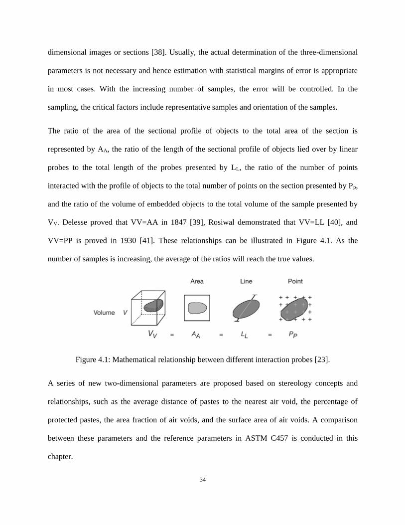
The ratio of the area of the sectional profile of objects to the total area of the section is
represented by AA, the ratio of the length of the sectional profile of objects lied over by linear
probes to the total length of the probes presented by LL, the ratio of the number of points
interacted with the profile of objects to the total number of points on the section presented by Pp,
and the ratio of the volume of embedded objects to the total volume of the sample presented by
VV. Delesse proved that VV=AA in 1847 [39], Rosiwal demonstrated that VV=LL [40], and
VV=PP is proved in 1930 [41]. These relationships can be illustrated in Figure 4.1. As the
number of samples is increasing, the average of the ratios will reach the true values.
Figure 4.1: Mathematical relationship between different interaction probes [23].
A series of new two-dimensional parameters are proposed based on stereology concepts and
relationships, such as the average distance of pastes to the nearest air void, the percentage of
protected pastes, the area fraction of air voids, and the surface area of air voids. A comparison
between these parameters and the reference parameters in ASTM C457 is conducted in this
chapter.

35
4.1 The Entrained Air-void System and Spacing Factor
Entrained air is distributed in the paste as fine bubbles and the structure of the air-void system is
critical to guarantee the frost resistance. The spacing factor is one of the most critical parameters
of a satisfactory air void system, which is defined as the average distance from any point in the
paste to the edge of the nearest void to ensure adequate freezing protection. The air void spacing
equations have been proposed by a number of researchers: Powers, Philleo, Attiogbe, and Pleau
and Pigeon. The true spacing is attempted to be characterized by these spacing equations.
The structure of the air-void system is essential to obtain satisfactory frost resistance. Tiny
bubbles entrained are dispersed throughout the paste with an approximately spherical shape and
diameter from 0.05 mm to 1.25 mm [1]. The critical parameters of a satisfactory air-void system
are the spacing factor, specific surface area, and bubble frequency according to ASTM C 457.
The specific surface area and bubble frequency are interrelated and used to reflect the mean size
of the bubbles while the spacing factor which is introduced above is the average distance from
any point in the paste to the edge of the nearest void. The spacing factor is the most commonly
used parameter to ensure adequate freezing-thawing protection. A well-distributed system of
small bubbles could protect the entire paste volume and quantitative microscopic examination
can be conducted to determine these parameters using automated computer-based systems.
With the same air content, it could be expected that different air void spacing should exhibit
different freezing-thawing performance. Therefore, an air-void system could be characterized by
estimating some measure of air void spacing. A number of equations attempts to characterize the
air void spacing in air-entrained concrete, which will be discussed below.
For nomenclature for air void quantities in different equations, a set of common notation is used
to express quantities and given below:

36
n: number of air voids per volume
A: air void volume fraction
p: paste volume fraction
α: specific surface area of spheres
r: sphere radii
f(r): sphere radii probability density function
<Rk> : the expected value of Rk for the radius distribution
s: spacing distribution parameter.
Quantities of the paste-air systems can be defined in Equations 18-21:
34A n R
3
(18)
p 1-A (19)
2
3
4 n R
4 nR
3
(20)
0( )k kR r f r dr
(21)
4.1.1 Powers Spacing Factor
The most widely used spacing factor equation is the Powers spacing factor [16]. The air voids
are entrapped or entrained into the paste and some fraction of the paste could be protected by
these air voids within some distance. The distance of the paste from the surface of the air bubbles

37
is estimated, but the value of the paste fraction cannot be quantified. To develop the Power
spacing factor, two idealized systems are employed. If the p/A ratio is small, all of the paste is
assumed to spread into a uniformly thick layer over every air void when. If the p/A ratio is
relatively large, the cubic lattice approach is used and all air voids are supposed to have the same
size. Therefore, the resulting spacing factor can be estimated using the distance from the center
of the cubic cell to the nearest air void surface. The equations are shown below.
2/ 4.342
4
p pL p A
An R (22)
1/33
1.4 1 1 / 4.342p
L p AA
(23)
When the p/A equals 4.342, these two equations will have the same value of the spacing factor.
4.1.2 Philleo Spacing Equation
Philleo extended the Powers’ approach by quantifying the volume fraction of the paste within a
distance from an air void [42]. Philleo spacing equation has an ideal air void system with
randomly distributed points with known statistics and then modified to account for finite-sized
spheres. The result characterizes the spacing of the paste to the finite-sized air voids. For a paste-
void system, the Philleo spacing factor estimates the volume fraction of paste within a distance s
from an air void surface [42]:
3 2 1/3 2/3( ) 1 exp[ 4.19x 7.80x [ln(1/ ) 4.84 [ln(1/ )] ]F s p x p (24)
Where the substitution x=sn1/3 has been made.

38
4.1.3 Attiogbe Spacing Equation
Attiogbe [43] proposed a spacing equation to estimate the mean spacing of air voids in concrete.
In this equation, geometric probability concepts and stereological principles are used to derive
the mean spacing of air voids.
2
2p
tA
(25)
By a numerical test, Attiogbe suggested that the equation is valid for all values of paste-to-air
ratio, p/A and the mean spacing yields a better estimate of the actual spacing of the air voids in
hardened concrete than the Powers spacing factor.
4.1.4 Mean Free Path
The mean free path is calculated by the average chord lengths in the paste, which is determined
by Equation 26 [44]:
2
p
n R
(26)
If the centers of the air voids are fixed, as the radii of these air voids are decreasing to zero, the
mean free path changes to infinity, which equals to t in the Attiogbe equation. In fact, t in the
Attiogbe equation is directly proportional to λ [44]. The Attiogbe equation t can be expressed as:
22
2 2
p p p pt p
A n R
(27)
Therefore, t in the Attiogbe equation approximately equals to half of the mean free path in a
paste-void system.
39
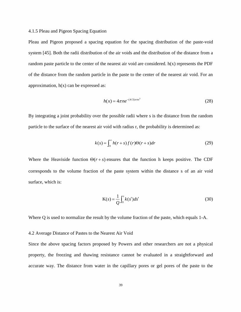
4.1.5 Pleau and Pigeon Spacing Equation
Pleau and Pigeon proposed a spacing equation for the spacing distribution of the paste-void
system [45]. Both the radii distribution of the air voids and the distribution of the distance from a
random paste particle to the center of the nearest air void are considered. h(x) represents the PDF
of the distance from the random particle in the paste to the center of the nearest air void. For an
approximation, h(x) can be expressed as:
3(4/3)( ) 4 nxh x ne (28)
By integrating a joint probability over the possible radii where s is the distance from the random
particle to the surface of the nearest air void with radius r, the probability is determined as:
0( ) ( ) ( ) ( )k s h r s f r r s dr
(29)
Where the Heaviside function ( )r s ensures that the function h keeps positive. The CDF
corresponds to the volume fraction of the paste system within the distance s of an air void
surface, which is:
0
1K( ) ( )
s
s k s dsQ
(30)
Where Q is used to normalize the result by the volume fraction of the paste, which equals 1-A.
4.2 Average Distance of Pastes to the Nearest Air Void
Since the above spacing factors proposed by Powers and other researchers are not a physical
property, the freezing and thawing resistance cannot be evaluated in a straightforward and
accurate way. The distance from water in the capillary pores or gel pores of the paste to the

40
nearest air void is of importance to indicate the true spacing factor. This distance in fact
represents how far the water needs to travel to air voids.
Based on the novel method to determine the parameters using flatbed scanners, the three-phase
image of concrete sections can be obtained. All pastes pixels can be displayed in gray color in
the image. Therefore, the distance of pastes axils to the nearest air void could be used to
determine the distance of water in capillary pores or gel pores to the nearest air void. The air
void pixels are displayed in white color in the three-phase image. Matlab can be used in this
calculating process since the three-phase image can be easily imported in the Matlab and
converted into matrix. For a grayscale image, black pixels are converted into 0, white pixels into
255, and gray pixels into the rest number in the matrix. In this situation, aggregates are converted
into 0, air voids into 255, and pastes into the rest number in the matrix. If the matrix of the three-
phase image is obtained, a large enough area is given from each pastes pixel. Within the area, the
distances from the paste pixel to all air voids pixels are calculated and the minimum distance is
then recorded. All minimum distances of all pastes pixels are averaged to characterize the
spacing factor. However, in the scanning image, about 1 million × 1 million pixels are collected
and about 20 million pixels are cement pastes. If all minimum distances of all these pastes pixels
are exported and saved, a large number of data are not easy to manage. More importantly, there
is no need to analyze all the distances since the distribution and the average value of the
distances are what we concern. Therefore, the whole scanning image along with the three-phase
image of concrete sections is divided into 50×50 parts and the average minimum distance of
pastes pixels in each part is exported. The distribution of average distance of these 2500 parts
indicates the distribution of all distance of pastes pixels in the three-phase image and the average
of the 2500 distances indicates the average of all pastes pixels. In Table 4.1, the error of the

41
estimation is shown for the average distance of the 2500 parts. Table 4.1 indicates that the largest
error is less than 8% and most of the errors are below 5%. The samples from CTLGroup are
analyzed to determine the new spacing factor and the results will be introduced in the following
part.
Table 4.1: Error of the estimation for the average distance of the 2500 parts.
Sample Average distance (µm)
Error Average of all pastes Average of 1500 parts
A1 150.53 157.5985 4.70%
A2 118.03 127.2189 7.78%
A3 122.15 122.7995 0.53%
A4 125.26 130.4589 4.15%
B1 126.13 133.0157 5.46%
B2 142.14 150.0286 5.55%
B3 112.35 116.6622 3.84%
B4 135.72 140.4461 3.49%
E1 95.99 96.3043 0.33%
E2 129.72 130.8897 0.90%
E3 101.38 99.9617 1.40%
E4 111.42 111.2188 0.18%
F1 81.72 76.3690 6.55%
F2 71.61 68.1956 4.77%
F3 95.98 95.5768 0.42%
F4 86.68 85.0778 1.85%
For sample E3, the cumulative relative frequency of the average distance in the 2500 parts is
shown in Figure 4.2. It can be seen that 90% of average distances are below 140 µm and 50%
below about 90 µm. The average distance of E3 is calculated and equals to 101.38 µm. Although
the value of the spacing factor is small enough for a good freezing and thawing resistance, there

42
are some areas whose average distance of pastes pixels to the nearest air voids exceeds 200 µm
or even 250 µm.
Figure 4.2: Cumulative relative frequency of the average distance of E3.
Another advantage of the method that the three-phase image is divided into 50×50 parts and
analyzed using Matlab is that the areas with larger average distances can be picked out. In Figure
4.3, the red areas have the average distance greater than 250 μm. For sample E3, the easily
damaged areas are on the edge of some coarse aggregates. Most of some red areas, for example
the two areas on the lower right corner, locate on coarse aggregates, but some pastes pixels can
be seen when the image is zoomed in. Since no air voids in coarse aggregates or no passing
channel to coarse aggregates is assumed, the water in the pastes on the edge of coarse aggregates
0%
10%
20%
30%
40%
50%
60%
70%
80%
90%
100%
0 50 100 150 200 250 300 350 400 450
Cu
mu
lati
ve r
elat
ive
freq
uen
cy
Average distance (μm)
Cumulative relative frequency of the average distance

43
can only flow towards other directions. Therefore, some easily damaged areas may be on the
edge of coarse aggregates.
Figure 4.3: Easily damaged areas of E3.
For sample B4, the cumulative relative frequency of the average distance can be shown in Figure
4.4. It can be seen that 90% of average distances are below 220 µm and 50% below about 125
µm. The average distance of E3 equals to 135.72 µm. Compared with sample E3, the average
distance of sample B4 is larger and more areas in sample B4 have the average distance more than
250 µm. The easily damaged areas of B4 are shown in red in Figure 4.5.

44
Figure 4.4: Cumulative relative frequency of the average distance of B4.
0%
10%
20%
30%
40%
50%
60%
70%
80%
90%
100%
0 50 100 150 200 250 300 350 400 450
Cu
mu
lati
ve r
elat
ive
freq
uen
cy
Average distance (μm)
Cumulative relative frequency of the average distance

45
Figure 4.5: Easily damaged areas of B4.
Besides the areas on the edge of some coarse aggregates, the red areas locate where fine
aggregates and pastes crowd together without enough entrained air. In Figure 4.6, the magnified
areas with the average distance larger than 250 µm are shown.

46
Figure 4.6: Magnified easily damaged areas of B4.
Sample A1 to A4, B1 to B3, E1, E2, E4, and F1 to F4 are all analyzed to obtain the cumulative
relative frequency of the average distance and the new spacing factor. The cumulative relative
frequency curve will be shown in Appendix C, while the spacing factor will be summarized in
Table 4.2. In Table 4.2, the spacing factor according to ASTM C457 will also be shown for
comparison. It can be observed in Figure 4.7 that spacing factor in ASTM C457 is always larger
than the average distance for a given sample. The method in ASTM C457 to determine the
spacing factor is based on one-dimensional chord line calculation so that the air voids that are not
traversed are ignored for protection on the cement pastes. Thus, the spacing factor in ASTM
C457 is higher and the freezing and thawing resistance for the concrete samples is
underestimated.

47
Table 4.2: Comparison of spacing factor in ASTM C457 and average distance.
Sample
Spacing Factor in ASTM C457
Average distance
(inch) (µm) (inch)
A1 0.0059 150.53 0.0059
A2 0.0050 118.03 0.0046
A3 0.0058 122.15 0.0048
A4 0.0071 125.26 0.0049
AAverage 0.0059 128.99 0.0051
B1 0.0064 126.13 0.0050
B2 0.0066 142.14 0.0056
B3 0.0071 112.35 0.0044
B4 0.0075 135.72 0.0053
BAverage 0.0069 129.08 0.0051
E1 0.0049 95.99 0.0038
E2 0.0059 129.72 0.0051
E3 0.0054 101.38 0.0040
E4 0.0060 111.42 0.0044
CAverage 0.0055 109.63 0.0043
F1 0.0024 81.72 0.0032
F2 0.0039 71.61 0.0028
F3 0.0050 95.98 0.0038
F4 0.0050 86.68 0.0034
DAverage 0.0041 84.00 0.0033

48
Figure 4.7: Comparison of spacing factor in ASTM C457 and average distance.
The average air content versus the average distance for each sample group is shown in Table 4.3.
It can be seen that even though the air content of two samples are similar, the average distance
may be different. Moreover, the sample whose air content is lower may also have lower average
distance. Therefore, air content alone is insufficient to estimate the freezing and thawing
resistance.
0.0000
0.0010
0.0020
0.0030
0.0040
0.0050
0.0060
0.0070
0.0000 0.0010 0.0020 0.0030 0.0040 0.0050 0.0060 0.0070 0.0080
Ave
rage
dis
tan
ce (
inch
)
Spacing factor in ASTM C457 (inch)
Spacing factor in ASTM C457 vs. average distance

49
Table 4.3: The average air content versus the average distance for each sample group.
Sample Air content
Average distance
(%) (µm)
AAverage 7.75 128.99
BAverage 6.96 129.08
CAverage 5.04 109.63
DAverage 6.35 84.00
4.3 Protected Paste
Based on stereology relationships, the volume of paste within a distance from air voids in a unit
volume can be determined by the average area ratio of paste on the sectional probes. Matlab was
used to measure the distance from every paste pixel to the nearest air void. According to ASTM
C457, a maximum value of 200 µm for the spacing factor is an appropriate criteria for moderate
exposure to freezing and thawing of concrete. Therefore, 200 µm is selected as the distance from
the periphery of air voids and the paste within the distance to be assumed to be protected by the
air voids. The area fraction of the protected paste can be calculated by the ratio of the number of
pastes pixels within the distance to the total number of paste pixels. In Table 4.4, the area
fraction of the protected paste is shown for the samples from CTLGroup. The specific surface
calculated according to ASTM C457 is also presented in Table 4.4. With larger specific surface
of air voids, the fraction of pastes within the selected distance from air voids should increase at
the same time. In Figure 4.8, the relationship between the fraction of protected pastes and the
specific surface in ASTM C457 is shown for the samples from CTLGroup.

50
Table 4.4: Area fraction of the paste within 200 µm from air voids.
Sample
Specific Surface in ASTM C457
Protected paste
(1/inch) (%)
A1 749.31 77.88%
A2 663.99 87.10%
A3 732.58 89.92%
A4 664.95 86.78%
AAverage 702.71 85.42%
B1 691.73 87.12%
B2 651.32 81.07%
B3 692.74 92.28%
B4 698.09 82.80%
BAverage 683.47 85.82%
E1 879.01 93.81%
E2 1071.51 85.51%
E3 1030.63 94.70%
E4 839.95 91.73%
CAverage 955.27 91.44%
F1 1462.17 98.03%
F2 858.80 98.88%
F3 1081.77 94.95%
F4 1053.69 96.54%
DAverage 1114.11 97.10%

51
Figure 4.8: Relationship between the specific surface and protected paste.
From Figure 4.8, the correlation is shown between the percentage of protected paste and the
conventional specific surface. The points are distributed intensively within the vicinity of the
trend line. If the area fractions of protected pastes and the specific surfaces are averaged for
Group A, B, E, and F, a good correlation is illustrated in Figure 4.9. Although the area fraction is
only a two-dimensional parameter indicating the true three-dimensional property, it loses less
information than the one-dimensional parameter like the specific surface since the specific
surface is calculated based on average chord length in ASTM C457.
0.00%
20.00%
40.00%
60.00%
80.00%
100.00%
120.00%
0.00 200.00 400.00 600.00 800.00 1000.00 1200.00 1400.00 1600.00
pro
tect
ed p
aste
(%
)
Specific surface in ASTM C457 (1/inch)
Specific surface in ASTM C457 vs. protected paste

52
Figure 4.9: Relationship between the average specific surface and average protected paste for
Group A, B, E, and F.
4.4 Area Fraction of Air Voids
The air content in volume of hardened concrete is represented by the ratio of the traverse length
through air voids to the total length of the linear probes in ASTM C457. If the amount of
sampling is large enough or the length of the linear probes is long enough in this case, the
margins of error will be controlled properly. Since the area fraction of air voids can be
determined easily and conveniently using the scanning image along with its three-phase image,
the air content can be represented by the area fraction of air voids on the image. In Table 4.5, the
comparison of the air content in ASTM C457 and area fraction of air voids on the scanning
image of samples from CTLGroup is shown. It can be seen that the error between the one-
0.00%
10.00%
20.00%
30.00%
40.00%
50.00%
60.00%
70.00%
80.00%
90.00%
100.00%
0.00 200.00 400.00 600.00 800.00 1000.00 1200.00
pro
tect
ed p
aste
(%
)
Specific surface in ASTM C457 (1/inch)
Specific surface in ASTM C457 vs. protected paste

53
dimensional and two-dimensional parameter is small when the amount of sampling is large
enough.
Table 4.5: Comparison of the air content in ASTM C457 and area fraction of air voids.
Case Air content in ASTM C457 [%] Area fraction [%] Error
A1 6.87 6.88 0.18%
A2 8.97 8.89 0.91%
A3 8.19 8.03 1.96%
A4 6.95 6.94 0.10%
B1 6.56 6.58 0.31%
B2 7.97 8.06 1.18%
B3 7.2 7.10 1.42%
B4 6.12 6.05 1.11%
E1 6.57 6.70 1.94%
E2 3.56 3.61 1.40%
E3 4.78 4.85 1.41%
E4 5.26 5.22 0.81%
F1 6.22 6.23 0.23%
F2 8.88 8.73 1.74%
F3 4.3 4.09 5.12%
F4 6.01 6.01 0.02%
4.5 Surface Area of Air Voids
The surface area of air voids is important to achieve a good freezing and thawing performance
for concrete no matter according to the Powers’ mechanism or the Chatterji mechanism of
freezing action. The larger specific surface, the more water in the paste within a distance from air
voids can be sucked into the air voids. Besides, the larger specific surface, the more water can
freeze on the inner layer of air voids before the unfrozen water is stopped flowing into the air
voids. The true surface area of air voids is a three-dimensional property of hardened concrete and
the relationship between the specific surface and an estimate with a two-dimensional probe, a
54
section has to be constructed. According to the results from West [24], the surface area of air
voids in a unit volume of hardened concrete can be determined by the ratio of the perimeter of air
voids on the section to the total area of the section, which is shown in Equation 31.
4SV AP
(31)
Where SV is the surface area of air voids in a unit volume of hardened concrete and PA is the
ratio of the perimeter of air voids on the section to the total area of the section.
The results of the perimeter and the resulting surface area of air voids in a unit volume for
samples from CTLGroup are shown in Table 4.6. The calculated specific surface in ASTM C457
for these samples is also shown.

55
Table 4.6: Comparison of specific surface in ASTM C457 and surface area of air voids in a unit
volume.
Case Specific Surface in ASTM C457 Perimeter Surface area
1/inch inch 1/inch
A1 749.3 162.1 53.3
A2 664.0 187.6 61.7
A3 732.6 181.5 59.6
A4 665.0 145.7 47.9
AAverage 702.7 169.2 55.6
B1 691.7 138.9 45.6
B2 651.3 153.6 50.5
B3 692.7 149.1 49.0
B4 698.1 134.5 44.2
BAverage 683.5 144.0 47.3
E1 879.0 179.4 59.0
E2 1071.5 115.8 38.1
E3 1030.6 148.4 48.8
E4 839.9 135.6 44.5
CAverage 955.3 144.8 47.6
F1 1462.2 229.6 75.4
F2 858.8 279.1 91.7
F3 1081.8 138.4 45.5
F4 1053.7 193.8 63.7
DAverage 1114.1 210.2 69.1
The relationship between specific surface in ASTM C457 and the surface area of air voids in a
unit volume of hardened concrete can be illustrated in Figure 4.10. The specific surface in
ASTM C457 is defined as “the surface area of the air voids divided by their volume” [2] and it
indicates the size of air bubbles. However, the specific surface does not consider the interval
between air voids and it is not a parameter associated with the mechanism of freezing. Instead,
surface area of air voids in a unit volume of hardened concrete evaluates the amount of water

56
that can be sucked into air voids along with the amount of pastes that can be protected. Therefore,
surface area of air voids in a unit volume can be utilized to represent the freezing and thawing
performance of concrete directly.
Figure 4.10: Relationship between specific surface in ASTM C457 and surface area of air voids.
In Figure 4.11, the specific surfaces and surface areas of air voids in a unit volume are averaged
for Group A, B, E, and F and the discreteness of the points decreases. The specific surface could
be expected to increase with the increasing air content and the surface area of air voids in a unit
volume also increases with the air content. Then, a correlation between specific surface in ASTM
C457 and surface area of air voids in a unit volume should exist as shown in Figure 4.11.
0.0
10.0
20.0
30.0
40.0
50.0
60.0
70.0
80.0
90.0
100.0
0.0 200.0 400.0 600.0 800.0 1000.0 1200.0 1400.0 1600.0
Surf
ace
area
(1
/in
ch)
Specific surface in ASTM C457 (1/inch)
Specific surface in ASTM C457 vs. surface area

57
Figure 4.11: Relationship between the average specific surface and average surface area for
Group A, B, E, and F.
0.0
10.0
20.0
30.0
40.0
50.0
60.0
70.0
80.0
0.0 200.0 400.0 600.0 800.0 1000.0 1200.0
Surf
ace
area
(1
/in
ch)
Specific surface in ASTM C457 (1/inch)
Specific surface in ASTM C457 vs. surface area

58
Chapter 5. Conclusions
This study has developed new techniques and improved existing methods for measuring the
parameters of the air-void system. With the ASTM C457 test method serving as a reference,
new techniques and automated methods have been developed to acquire and analyze images of
polished sections of concrete. Specimen preparation methods were refined, using
phenolphthalein to stain the paste and an orange powder to fill air bubbles and provide high
brightness and image contrast. A high resolution flatbed scanner was used for image acquisition,
and procedures were developed so that a single image could be used for all aspects of analysis.
This key advancement makes image acquisition faster and avoids error arising from registration
of multiple images. Image processing methods using ImageJ, Photoshop, and Matlab were
developed.
The structure of the air-void system in hardened concrete mixed with air-entraining admixtures is
critical for the frost resistance of concrete. Mechanisms of freezing and thawing damage have
been explained by hydraulic pressure theory, energy of solidification theory, osmotic pressure
theory, Litvan’s theory, Chatterji’s theory, crystallization pressure theory, and cryo-suction
theory. Many contradictions between these theories exist, but in many respects, these theories
complement each other. Although debate continues regarding Powers hydraulic pressure theory,
the spacing factor proposed by Powers is today one of the most widely used parameters to
characterize the air-void system, and it has been demonstrated to be successful in practical work.
Many spacing factor equations including Powers equation have proposed to characterize the true
spacing of the air voids in hardened concrete, and this will be a subject of research for years to
come.

59
A “blind study” was completed to validate the new methods using ASTM C457 results as a
reference. The study demonstrated that new automated techniques could provide results
comparable to the traditional ASTM C457 test method while opening the door to two-
dimensional analysis.
This study proposes new two-dimensional parameters including the average distance of pastes to
the nearest air void, the percentage of protected pastes, the area fraction of air voids, and the
surface area of air voids. These parameters improve upon simple one-dimensional parameters for
addressing models and mechanisms of freezing and thawing performance of concrete. The three-
phase image obtained from the automated method makes it possible to determine these
parameters by dealing with the polished concrete sections. The relationships between these two-
dimensional parameters and the actual freezing and thawing performance should be the subject
of research in the future.
The methods in this study have limitations, and thus future work in this area is encouraged.
Aggregate porosity – particularly lightweight aggregates – remains a challenge for automated
segmentation of phases. Pore spaces such as air bubbles, air voids, and aggregate pores are
difficult to differentiate using automated methods. Further software and hardware development
may overcome these challenges in the future. Fortunately, these same factors can be shown to
have relatively low influence on the measured parameters of the air-void system, and the
averaged test results may not be greatly affected.

60
References
[1] Mindess, S, Young, J.F. and Darwin D., (2003) Concrete, 2nd ed., Prentice Hall, Upper
Saddle River, NJ.
[2] ASTM Standard C457, 2012, "Standard Test Method for Microscopical Determination of
Parameters of the Air-Void System in Hardened Concrete," ASTM International, West
Conshohocken, PA.
[3] Chatterji, S., and Gudmundsson, H., (1977) “Characterization of Entrained Air Bubble
System in Concrete by Means of an Image Analysis Microscope,” Cement and Concrete
Research, Vol. 7, No. 4, pp. 423-428.
[4] Pleau, R., Pigeon, M., Laurencot, J. L., (2001) “Some Findings on the Usefulness of Image
Analysis for Determining the Characteristics of the Air-void System on Hardened Concrete,”
Cement and Concrete Composites, Vol.23, pp. 237-246.
[5] Zhang, Z., Ansari, F. and Vitillo, N., (2005) “Automated Determination of Entrained Air
Void Parameters in Hardened Concrete,” ACI Materials Journal, Vol. 102, No. 1, Jan.-Feb.
[6] Schlorholtz, S., (1998) Image Analysis for Evaluating Air Void Parameters of Concrete,
Project HR-396, Final Report. Iowa Department of Transportation, Ames.
[7] Peterson, K. R., Swartz, R. A., Sutter, L. L., and Van Dam, T. L., (2002) “Hardened Concrete
Air Void Analysis with a Flatbed Scanner,” Journal of Transportation Research Board, No.
1775, Transportation Research Board, National Research Council, Washington, D.C., pp. 36-
43.
[8] Zalocha, D., Kasperkiewicz, J., (2005) “Estimation of the structure of air entrained concrete
using a flatbed scanner,” Cement and Concrete Research, 35 (10), pp. 2041-2046.
[9] Peterson, K., L. Sutter, and Radlinski, M., (2009) "The Practical of Application a Flatbed
Scanner for Air-Void Characterization of Hardened Concrete," Journal of ASTM
International, Vol. 6.

61
[10] Peterson, K., J. Carlson, L. Sutter, and Van Dam, T., (2009) "Methods for Threshold
Optimization for Images Collected from Contrast Enhanced Concrete Surfaces for Air-
Void System Characterization," Materials Characterization, Vol. 60, pp. 710-715.
[11] Radlinski, M., Olek, J., Zhang, Q.and Peterson, K., (2010) "Evaluation of the Critical Air-
Void System Parameters for Freeze-Thaw Resistant Ternary Concrete using the Manual
Point-Count and the Flatbed Scanner Methods," Journal of ASTM International, Vol. 7.
[12] Zalocha, D., and Kasperkiewicz, J., “Estimation of the Structure of Air Entrained Concrete
Using a Flatbed Scanner,” Cement and Concrete Research, Vol. 35, 2005, pp. 2041-2046.
[13] Jakobsen, U. H., Pade, C., Thaulow, N., Brown, D., Sahu, S., Magnusson, O., De Buck, S.,
and De Schutter, G., (2006) "Automated Air Void Analysis of Hardened Concrete - a
Round Robin Study," Cement and Concrete Research, Vol. 36, pp. 1444-1452.
[14] Ramezanianpour, A. M. and Hooton, R. D., (2010) "Evaluation of Two Automated Methods
for Air-Void Analysis of Hardened Concrete," ASTM Special Technical Publication Vol.
1511, pp. 27-40.
[15] Ramezanianpour, A. A., Nadooshan, M. J., and Peydayesh, M., (2013) "Effect of New
Composite Cement Containing Volcanic Ash and Limestone on Mechanical Properties and
Salt Scaling Resistance of Concrete," Journal of Materials in Civil Engineering, Vol.25, pp.
1587-1593.
[16] Powers, T.C., (1949) “The air requirement of frost-resistant concrete,” Proceedings of the
Highway Research Board, 29, 184-211.
[17] Powers, T.C. and Helmuth, R.A., (1953) “Theory of volume changes in hardened Portland
cement pasts during freezing,” Proceedings of the Highway Research Board, 32, 285-297.
[18] Powers, T.C., (1975) “Freezing effects in Concrete,” ACI Special Publication SP-47,
American Concrete Institute, Detroit, MI, pp. 1-11.
[19] Litvan, G.G., (1972) “Phase transitions of adsorbates IV ─ Mechanism of frost action in
hardened cement paste,” Journal of the American Ceramic Society, 55(1), 38-42.

62
[20] Chatterji, S., (2003) “Freezing of air-entrained cement-based materials and specific actions
of air-entraining agents,” Cement Concrete Composite, 25 (7) pp. 759–765.
[21] Scherer, G.W. and Valenza II, J.J., “Mechanisms of Frost Damage,” Materials Science of
Concrete, Vol. VII, pp. 209-246.
[22] Coussy, Olivier, Monteiro, Paulo, (2008) “Poroelastic model for concrete exposed to
freezing temperatures,” Cement and Concrete Research, Volume 38, Issue 1, Pages 40-48.
[23] West, Mark J., (2012) Basic Stereology for Biologists and Neuroscientists, CSHL Press,
Cold Spring Harbor, NY, USA.
[24] West, MJ., (1993) “New stereological methods for counting neurons,” Neurobiol Aging, 14,
275–285.
[25] Defay, R. and Prigogine, I., (1966) Surface Tension and Adsorption, Wiley, New York.
[26] Brun, M., Lallemand, A., Quinson, J.F., Eyraud, C., (1977) “A new method for the
simultaneous determination of the size and the shape of pores: the thermoporometry”,
Thermochimica Acta, 21, 59-88.
[27] Everett, D.H. and Haynes, J.M., (1965) “Capillary properties of some model system with
special reference to frost damage,” RILEM. Bull., 168, 65-73.
[28] Pigeon, M. and Pleau, R., (1994) Durability of Concrete in Cold Climates, Chapman and
Hall, London.
[29] Chatterji, S., (1999) “Aspects of freezing process in porous material–water system. Part 2.
Freezing and properties of frozen porous materials,” Cement and Concrete Research,
29,781–4.
[30] Helmuth, RA., (1961) “Dimensional changes of hardened Portland cement pastes caused by
temperature changes,” Proceedings of Highway Research Board, 40, 315–36.
[31] Helmuth, RA., (1960) “Capillary size restriction on ice formation in hardened Portland
cement pastes,” Proceedings of the IV International Symposium on Chemistry of Cement,
Washington DC, vol. II., p. 855–69.

63
[32] Helmuth, RA., (1960) “Discussion of the paper ‘Frost action in concrete.’ by P. Nerenst,”
Proceedings of the IV International Symposium on Chemistry of Cement, Washington DC,
vol. II., p. 829–33.
[33] Mielenz, RC., (1968) “Use of surface-active agents in concrete,” Proceedings of the V
International Symposium on Chemistry of Cement, Tokyo, Part IV. p. 1–102.
[34] Chatterji, S., (1984) “The spacing factor in entrained air-bubbles. Has it any significance?”
Cement and Concrete Research, 14,757–8.
[35] ASTM C233, 2011, “Air-entraining admixtures for concrete. American Society for Testing
Materials,” ASTM International, West Conshohocken, PA.
[36] ASTM C260, 2010a, “Standard specification for air-entraining admixtures for concrete,”
American Society for Testing Materials, ASTM International, West Conshohocken, PA.
[37] Monteiro, P.J.M., Coussy, O., Silva, D. A., (2006) “Effect of cryo-suction and air void
transition layer on hydraulic pressure of freezing concrete,” Materials Journal, ACI, 103 (2)
136–140.
[38] Weibel, ER., (1979) Stereological methods Vol 1: Practical methods for biological
morphometry, Academic Press, London.
[39] Delesse, MA., (1847) “Procédé mécanique pour déterminer la composition des roches,”
Comptes Rendus de l'Académie des Sciences, 25, 544–545.
[40] Rosiwal, A., (1898) “Über geometrische Gesteinsanalysen,” Verhandl der KK Geol.
[41] Thomson, E., (1930) “Quantitative microscopic analysis,” The Journal of Geology, 38, 193–
222.
[42] Philleo, R.E., (1983) “A method for analyzing void distribution in air-entrained concrete,”
Cement and Concrete Aggregates, 5, 128-130.
[43] Attiogbe, E.K., (1993) “Mean spacing of air voids in hardened concrete,” ACI Materials
Journal, 90, 174-181.
[44] Underwood, E.E., (1970) Quantitative Stereology, Addison-Wesley, Reading.

64
[45] Pleau, R. and Pigeon, M., (1996) “The use of the flow length concept to assess the
efficiency of air entrainment with regards to frost durability: Part - Description of the test
method,” Cement and Concrete Aggregates, 18, 19-29.

65
Appendix A. Experimental Procedure of the Automated Measurement of the
Parameters of Air-void System
Sample Preparation
The procedures to prepare samples for scanning reflect guidance and recommendations from
other researchers, including Kyle Riding (KSU), Karl Peterson (Toronto), and Kim Kurtis
(Gatech).
Sectioning:
Cut a sample that is of uniform thickness (about 2 inches) using a concrete saw. It is important
for the subsequent polishing process to cut a sample of uniform thickness since fewer and
shallow scratches from the saw cut lead to less effort in the first polishing step. During the cut,
water is used to move the dirt from the sample.
Figure A.1: (Left) Concrete saw; (Right) Cut a sample with uniform thickness.

66
Air Void Protection:
After washing the sample from sectioning with water, apply lacquer to the surface and let dry to
protect the air voids on the surface. In order to check if the sample is polished uniformly, draw
circles on the sample using a construction crayon before polishing.
Figure A.2: Air void protection.
Sample Holder Frame:
A wooden frame is made to hold samples and the holes in the frame are slightly larger than 4-
inch diameter cylinders. Bearings and rollers are fixed underneath the frame to help samples in
rotating during polishing so that a smooth and uniform polishing surface is obtained. Samples are
required to rest higher than the level of the rollers in order to ensure contact between the samples
and rollers. The positions of the rollers need to be determined by iterative trial to ensure that
there is enough room for samples to rotate.

67
Figure A.3: Sample holder frame.
Polishing:
An 18 inch lapping wheel is used to polish samples; in this case a model ASW-1800
manufactured by ASW Diamond. A sequence of lapping disks are attached on the ground steel
plate and the polishing protocol is shown below:
60 grit disk (10 minutes)
260 grit disk (10 minutes)
800 grit disk (15-20 minutes)
Wash the samples between polishing steps.

68
Figure A.4: Polishing.
Cleaning and Checking Flatness:
After all polishing steps, the sample needs to be washed and dried using fan for 20 minutes. Then,
soak samples in pure lacquer thinner to remove the lacquer applied before polishing from the air
voids. After drying the samples, check the flatness of the surface with a machinist rule. If no
light can transmit through the contact surface, the flatness is satisfactory.
Figure A.5: Cleaning and checking flatness.
Staining:

69
1% solid phenolphthalein is dissolved in a 1:1 solution of methanol and water. Next, the polished
surface is stained with phenolphthalein solution using a sprayer. Allow the solution to sit for
about 1 min and dry the samples using a fan for 20 min.
Figure A.6: Staining.
Orange-Powder Treatment:
After staining, press orange marking chalk powder gently into the voids using a rubber stopper.
Next, scrape away most of the excess powder with a razor blade and wipe away the remaining
powder.
Figure A.7: Orange-powder treatment.

70
Scanning and Registration:
A Canon CanoScan 9000F scanner is used set at the highest resolution 4800 x 4800 dpi (or 5.3
microns per pixel). The sample is placed at the corner of the glass bed, about 1 inch from the two
edges. Scan only once and a tiff type image can be obtained. The area is 50×50 mm and image
size is about 255 MB. Scanning time is about 2 min.
Figure A.8: Scanning and registration.
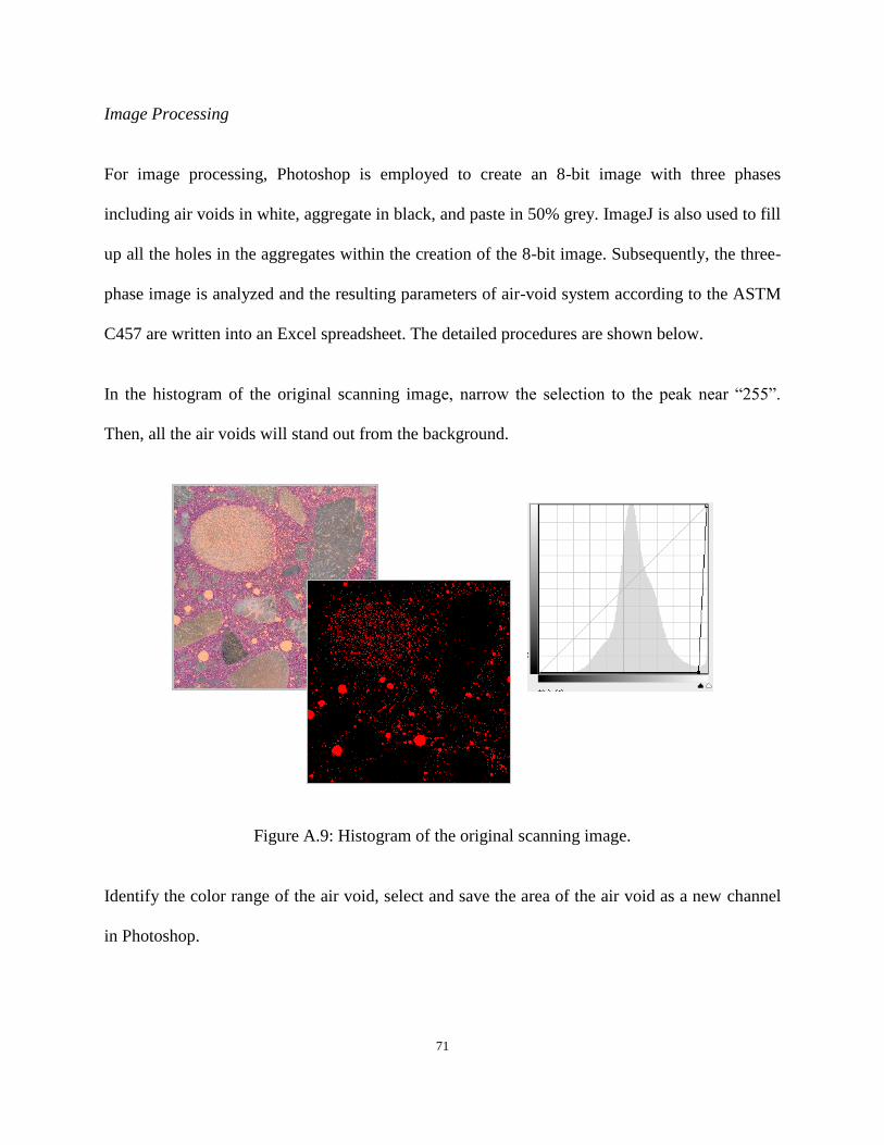
71
Image Processing
For image processing, Photoshop is employed to create an 8-bit image with three phases
including air voids in white, aggregate in black, and paste in 50% grey. ImageJ is also used to fill
up all the holes in the aggregates within the creation of the 8-bit image. Subsequently, the three-
phase image is analyzed and the resulting parameters of air-void system according to the ASTM
C457 are written into an Excel spreadsheet. The detailed procedures are shown below.
In the histogram of the original scanning image, narrow the selection to the peak near “255”.
Then, all the air voids will stand out from the background.
Figure A.9: Histogram of the original scanning image.
Identify the color range of the air void, select and save the area of the air void as a new channel
in Photoshop.

72
Figure A.10: Identification of the color range of the air void.
Use the channel mixer function to highlight all the air voids and aggregates and under this
adjustment, the paste is shown in black. Then, assign a new channel for the selected air voids and
aggregates.

73
Figure A.11: Highlight of the air voids and aggregates.
Create an 8-bit image and in this image, the selected air voids and aggregates are shown in black.
Then, subtract the air voids obtained in previous step from the 8-bit image so as to get a new
image only presenting the aggregates.
Figure A.12: 8-bit image presenting the aggregates.

74
Import the new 8-bit image into ImageJ and fill up all the holes in the aggregates. In the filling,
set the scale according to the sample conditions and filter out the aggregates less than 10 microns
in diameter. Select “Masks” in the dropdown list of “Show” and a new image of aggregates is
obtained.
Next, a three-phase image can be created with “air-voids” in white (255), “aggregates” in black
(0), and “paste” in 50% grey (128).
Figure A.13: Creation of a three-phase image.
The three-phase image is imported into Matlab and the resulting parameters of air-void system in
the sample according to ASTM C457 are written into an Excel spreadsheet.

75
Figure A.14: Calculation of the parameters in ASTM C457 using Matlab.

76
Appendix B. Original Scanning Images and Three-phase Images
Figure B.1: Scanned photo, A1. Figure B.2: Three-phase image, A1.
Figure B.3: Scanned photo, A2. Figure B.4: Three-phase image, A2.

77
Figure B.5: Scanned photo, A3. Figure B.6: Three-phase image, A3.
Figure B.7: Scanned photo, A4. Figure B.8: Three-phase image, A4.
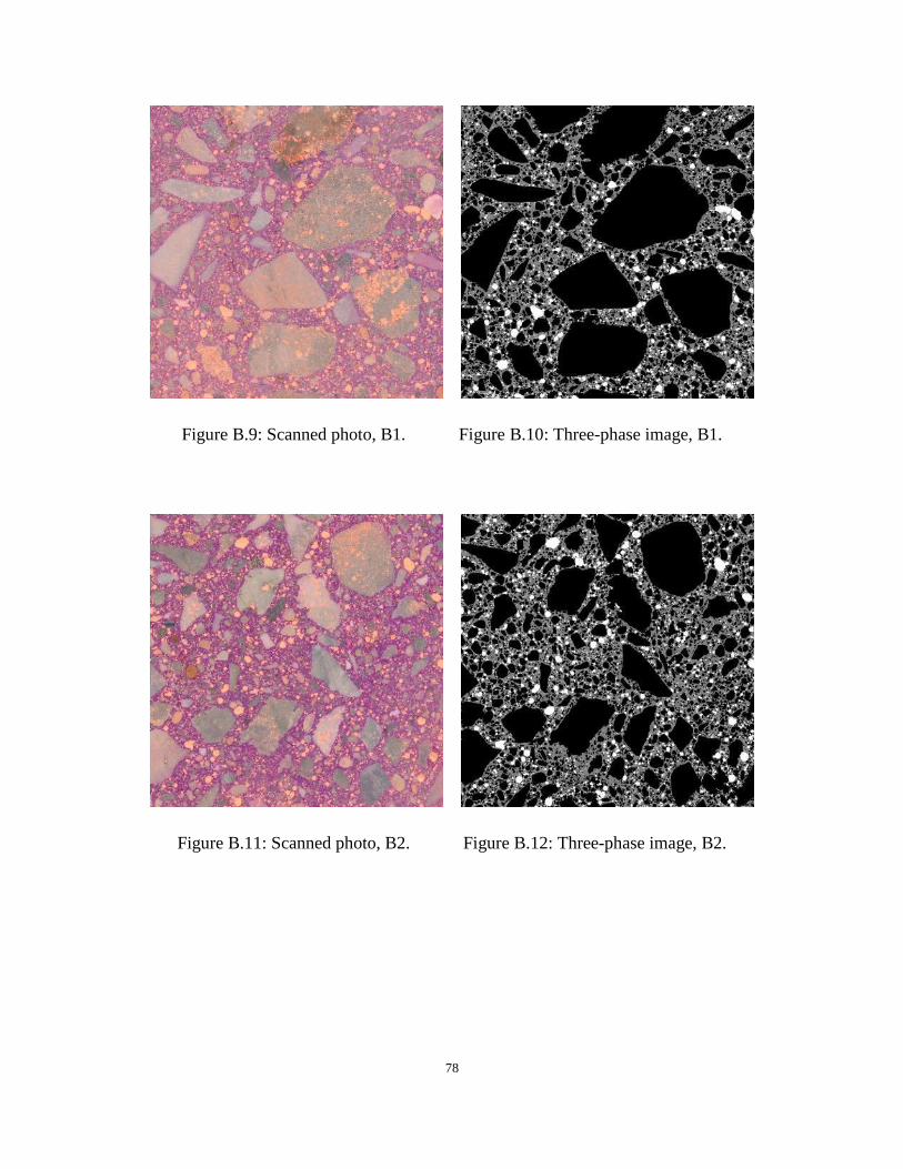
78
Figure B.9: Scanned photo, B1. Figure B.10: Three-phase image, B1.
Figure B.11: Scanned photo, B2. Figure B.12: Three-phase image, B2.

79
Figure B.13: Scanned photo, B3. Figure B.14: Three-phase image, B3.
Figure B.15: Scanned photo, B4. Figure B.16: Three-phase image, B4.

80
Figure B.17: Scanned photo, C1. Figure B.18: Three-phase image, C1.
Figure B.19: Scanned photo, C2. Figure B.20: Three-phase image, C2.

81
Figure B.21: Scanned photo, D1. Figure B.22: Three-phase image, D1.
Figure B.23: Scanned photo, D2. Figure B.24: Three-phase image, D2.

82
Figure B.25: Scanned photo, E1. Figure B.26: Three-phase image, E1.
Figure B.27: Scanned photo, E2. Figure B.28: Three-phase image, E2.

83
Figure B.29: Scanned photo, E3. Figure B.30: Three-phase image, E3.
Figure B.31: Scanned photo, E4. Figure B.32: Three-phase image, E4.

84
Figure B.33: Scanned photo, F1. Figure B.34: Three-phase image, F1.
Figure B.35: Scanned photo, F2. Figure B.36: Three-phase image, F2.

85
Figure B.37: Scanned photo, F3. Figure B.38: Three-phase image, F3.
Figure B.39: Scanned photo, F4. Figure B.40: Three-phase image, F4.
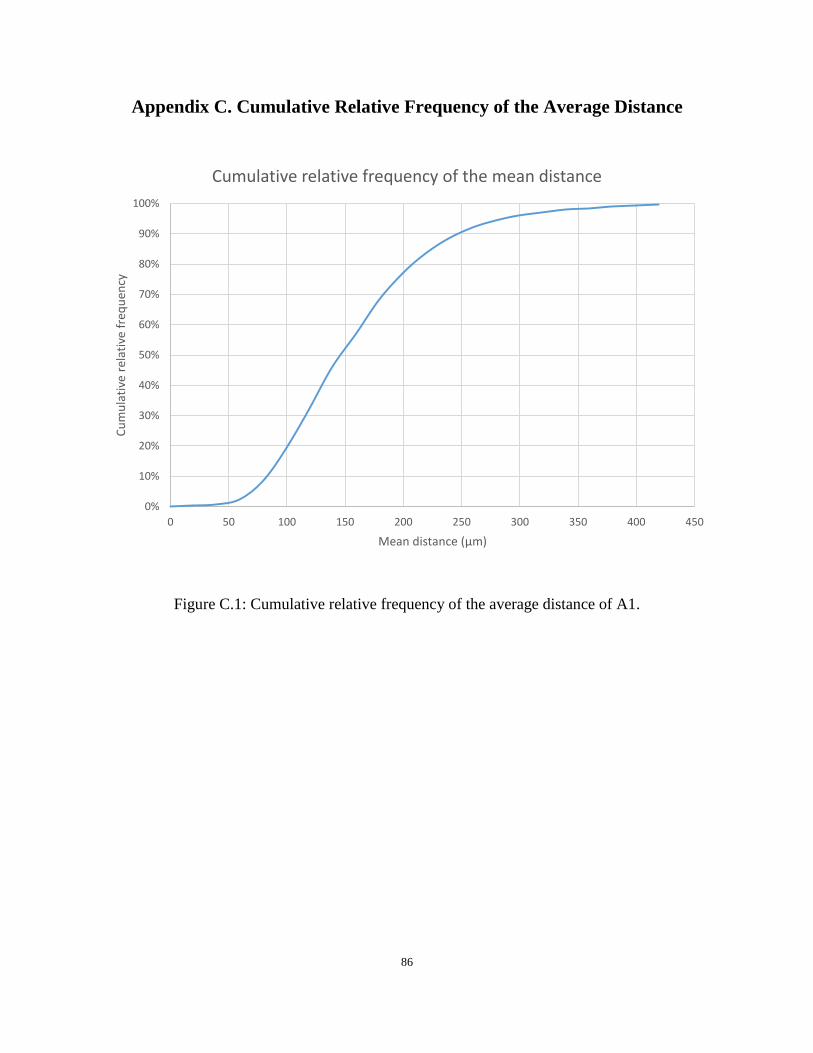
86
Appendix C. Cumulative Relative Frequency of the Average Distance
Figure C.1: Cumulative relative frequency of the average distance of A1.
0%
10%
20%
30%
40%
50%
60%
70%
80%
90%
100%
0 50 100 150 200 250 300 350 400 450
Cu
mu
lati
ve r
elat
ive
freq
uen
cy
Mean distance (μm)
Cumulative relative frequency of the mean distance

87
Figure C.2: Cumulative relative frequency of the average distance of A2.
0%
10%
20%
30%
40%
50%
60%
70%
80%
90%
100%
0 50 100 150 200 250 300 350 400 450
Cu
mu
lati
ve r
elat
ive
freq
uen
cy
Mean distance (μm)
Cumulative relative frequency of the mean distance

88
Figure C.3: Cumulative relative frequency of the average distance of A3.
0%
10%
20%
30%
40%
50%
60%
70%
80%
90%
100%
0 50 100 150 200 250 300 350 400 450
Cu
mu
lati
ve r
elat
ive
freq
uen
cy
Mean distance (μm)
Cumulative relative frequency of the mean distance

89
Figure C.4: Cumulative relative frequency of the average distance of A4.
0%
10%
20%
30%
40%
50%
60%
70%
80%
90%
100%
0 50 100 150 200 250 300 350 400 450
Cu
mu
lati
ve r
elat
ive
freq
uen
cy
Mean distance (μm)
Cumulative relative frequency of the mean distance

90
Figure C.5: Cumulative relative frequency of the average distance of B1.
0%
10%
20%
30%
40%
50%
60%
70%
80%
90%
100%
0 50 100 150 200 250 300 350 400 450
Cu
mu
lati
ve r
elat
ive
freq
uen
cy
Mean distance (μm)
Cumulative relative frequency of the mean distance

91
Figure C.6: Cumulative relative frequency of the average distance of B2.
0%
10%
20%
30%
40%
50%
60%
70%
80%
90%
100%
0 50 100 150 200 250 300 350 400 450
Cu
mu
lati
ve r
elat
ive
freq
uen
cy
Mean distance (μm)
Cumulative relative frequency of the mean distance

92
Figure C.7: Cumulative relative frequency of the average distance of B3.
0%
10%
20%
30%
40%
50%
60%
70%
80%
90%
100%
0 50 100 150 200 250 300 350 400 450
Cu
mu
lati
ve r
elat
ive
freq
uen
cy
Mean distance (μm)
Cumulative relative frequency of the mean distance

93
Figure C.8: Cumulative relative frequency of the average distance of E1.
0%
10%
20%
30%
40%
50%
60%
70%
80%
90%
100%
0 50 100 150 200 250 300 350 400 450
Cu
mu
lati
ve r
elat
ive
freq
uen
cy
Mean distance (μm)
Cumulative relative frequency of the mean distance

94
Figure C.9: Cumulative relative frequency of the average distance of E2.
0%
10%
20%
30%
40%
50%
60%
70%
80%
90%
100%
0 50 100 150 200 250 300 350 400 450
Cu
mu
lati
ve r
elat
ive
freq
uen
cy
Mean distance (μm)
Cumulative relative frequency of the mean distance

95
Figure C.10: Cumulative relative frequency of the average distance of E4.
0%
10%
20%
30%
40%
50%
60%
70%
80%
90%
100%
0 50 100 150 200 250 300 350 400 450
Cu
mu
lati
ve r
elat
ive
freq
uen
cy
Mean distance (μm)
Cumulative relative frequency of the mean distance

96
Figure C.11: Cumulative relative frequency of the average distance of F1.
0%
10%
20%
30%
40%
50%
60%
70%
80%
90%
100%
0 50 100 150 200 250 300 350 400 450
Cu
mu
lati
ve r
elat
ive
freq
uen
cy
Mean distance (μm)
Cumulative relative frequency of the mean distance

97
Figure C.12: Cumulative relative frequency of the average distance of F2.
0%
10%
20%
30%
40%
50%
60%
70%
80%
90%
100%
0 50 100 150 200 250 300 350 400 450
Cu
mu
lati
ve r
elat
ive
freq
uen
cy
Mean distance (μm)
Cumulative relative frequency of the mean distance

98
Figure C.13: Cumulative relative frequency of the average distance of F3.
0%
10%
20%
30%
40%
50%
60%
70%
80%
90%
100%
0 50 100 150 200 250 300 350 400 450
Cu
mu
lati
ve r
elat
ive
freq
uen
cy
Mean distance (μm)
Cumulative relative frequency of the mean distance

99
Figure C.14: Cumulative relative frequency of the average distance of F4.
0%
10%
20%
30%
40%
50%
60%
70%
80%
90%
100%
0 50 100 150 200 250 300 350 400 450
Cu
mu
lati
ve r
elat
ive
freq
uen
cy
Mean distance (μm)
Cumulative relative frequency of the mean distance