advanced wireless networking and cross-layer optimization

School of ECS, Univ. of Southampton, UK. http://www-mobile.ecs.soton.ac.uk 1/ 141 ⇒|

Advanced Wireless Networking and Cross-Layer OptimizationThe Myth of Interference-Free Communications...

Presented by

Lajos Hanzo

School of Electronics and Computer Science,

University of Southampton, SO17 1BJ, UK.

http://www-mobile.ecs.soton.ac.uk


Outline

❏ A historical perspective and information-theoretic limits

❏ Research drivers and contradictory design factor

❏ Multiple access techniques and their pros as well as cons

❏ Future-proof multi-carrier transceivers and systems

❏ The benefits and limitations of smart antennas/MIMOs: beamforming, SDMA, SDM as

well as STBC and STTC

❏ The benefits of smart TD, FD and SD spreading in multicarrier systems

❏ A digest of wireless networking considerations and the sensitivity of teletraffic

performance versus receiver SINR performance

❏ The required advanced transceivers and MBER optimization

❏ Improving the per-node capacity of ad hoc networks

❏ Conclusions and open problems


Figure 1: Instantaneous Channel SNR for all 512 subcarriers versus time, for an average

channel SNR of 16dB.


Research Drivers [1]-[9]:

• Researchers are endeavouring to reach information theoretical limits.

• Communications frequency bands have been auctioned at a price in excess of 75

Billion dollars in the US and 22 Billion pounds in the UK.

• Hence halving the bitrate doubles the revenue!

• Halving the bitrate requires exponentially increasing research efforts - BUT IT IS

FUN!

• Contradictory performance factors:

– ’Lossy’ source representation quality for audio, video, etc

– Bitrate

– Error resilience

– Implementation complexity

– Delay


Implementationalcomplexity

Channelcharacteristics

Effectivethroughput

bandwidthSystem Bit error

rate

Coding gain

schemeModulation

Coding/

Coding rate

Coding/interleavingdelay

Figure 2: Factors affecting the design of channel coding and modulation schemes [5]

c©John Wiley, 2001, Hanzo, Liew, Yeap.


1990

2000

1980

1970

1960

1950

Shannon limit (1948)

Elias, Convolutional codes

Viterbi algorithm

Bahl, MAP algorithm

Hamming codes

PGZ algorithm

Wolf, trellis block codes

Chase algorithm

Reed Solomon codesBCH codes

algorithmBerlekamp-Massey

RRNS codes

Ungerboeck, TCM

Berrou, turbo codes

Robertson, Log-MAP algorithm

Koch, Max-Log-MAP algorithmHagenauer, SOVA algorithm

Nickl, turbo Hamming codeHagenauer, turbo BCH code

Alamouti, space-timeblock code

Tarokh, space-time trellis codeRobertson, TTCM

Pyndiah, SISO Chasealgorithm

Convolutional CodesBlock Codes

Acikel, punctured turbo code

Figure 3: A brief history of channel coding [5].


Peterson & Weldon, Error correcting codes

Berlekamp, Algebraic coding theoryKasami, Combinational mathematics and its applications

Reed & Solomon, Polynomial codes over certain finite fields

1990

2000

1980

1970

1960

1950

Peterson, Error correcting codes

Mac Williams & Sloane, The theory of error correcting codes

Sklar, Digital communications fundamentals and applications

Blake, Algebraic coding theory: history and development

Clark & Cain, Error correction coding for digital communicationsPless, Introduction to the theory of error-correcting codesBlahut, Theory and practice of error control codes

Wozencraft & Reiffen, Sequential decodingShannon, Mathematical theory of communicationMassey, Threshold decoding

Shannon limit (1948)

Heegard & Wicker, Turbo coding

Bossert, Channel coding for telecommunicationsVucetic & Yuan, Turbo codes principles and applications

Lidl & Niederreiter, Finite fieldsLin & Costello, Error control coding: fundamentals and applicationsMichelson & Levesque, Error control techniques for digital communication

Steele & Hanzo, Mobile radio communications

Hoffman et al., Coding theoryHuber, TrelliscodierungAnderson & Mohan, Source and channel coding - an algorithmic approachWicker, Error control systems for digital Communication and storageProakis, Digital communicationsHonary & Markarian, Trellis decoding of block codesS. Lin et al., Trellises & trellis-based decoding alg. for linear block codesSchlegel, Trellis coding

Szabo & Tanaka, Residue arithmetic & its appl. to computer technology

Sweeney, Error Control Coding: An Introduction

Figure 4: Mile-stones in channel coding [5].


[1] L. Hanzo, W.T. Webb, T. Keller: Single- and Multi-carrier Quadrature Amplitude Modulation: Principles and Applications for

Personal Communications, WATM and Broadcasting; IEEE Press-John Wiley, 2000, p 739

(http://www-mobile.ecs.soton.ac.uk)

[2] R. Steele, L. Hanzo (Ed): Mobile Radio Communications: Second and Third Generation Cellular and WATM Systems,

John Wiley-IEEE Press, 2nd edition, 1999, ISBN 07 273-1406-8, p 1064

[3] L. Hanzo, F.C.A. Somerville, J.P. Woodard: Voice Compression and Communications: Principles and Applications for

Fixed and Wireless Channels; IEEE Press-John Wiley, 2001, p 642

[4] L. Hanzo, P. Cherriman, J. Streit: Wireless Video Communications: Second to Third Generation and Beyond, IEEE Press,

2001, p 1093

[5] L. Hanzo, T.H. Liew, B.L. Yeap: Turbo Coding, Turbo Equalisation and Space-Time Coding, John Wiley, 2002, p 751

[6] L. Hanzo, C.H. Wong, M.S. Yee: Adaptive wireless transceivers: Turbo-Coded, Turbo-Equalised and Space-Time Coded

TDMA, CDMA and OFDM systems, John Wiley, 2002, p 737

[7] J.S. Blogh, L. Hanzo: Third-Generation Systems and Intelligent Wireless Networking - Smart Antennas and Adaptive

Modulation, John Wiley, 2002, p 408

[8] L. Hanzo, M. Munster, B.J. Choi and T. Keller: OFDM and MC-CDMA for Broadband Multi-user Communications, WLANs

and Broadcasting, John Wiley - IEEE Press, May 2003, p 980

[9] L. Hanzo, L-L. Yang, E-L. Kuan and K. Yen: Single- and Multi-Carrier CDMA: Multi-User Detection, Space-Time

Spreading, Synchronisation, Standards and Networking, IEEE Press - John Wiley, June 2003, p950


The Standard-oriented Perspective on SDRs [9]

• The most recent version of the IMT-2000 standard is in fact constituted by a range of

five independent standards:

– UTRA Frequency Division Duplex (FDD) Wideband Code Division Multiple Access

(W-CDMA) mode

– UTRA Time Division Duplex (TDD) CDMA mode

– Pan-American multi-carrier CDMA configuration mode known as cdma2000

– Pan-American Time Division Multiple Access (TDMA) mode known as UWT-136

– Digital European Cordless Telecommunications (DECT) mode.

• It would be desirable to achieve that future systems become part of this standard

framework without having to define new standards, whilst also supporting legacy

systems, such as GSM, IS-95, etc. The framework proposed in this contribution is

capable of satisfying this requirement.


The Channel-quality Motivated Perspective on SDRs [9]

• Multiple Spreading Codes

• Variable Spreading Factors

• Variable Rate FEC Codes

• Different FEC Schemes: CC, BCH, TC, TBCH, TCM, TTCM, BICM, BICM-ID

• Turbo Channel Equaliser

• Variable Constellation Size: 1-6bit/symb

• Multiple Time Slots

• Multiple Bands

• Multiple Transmit Antennas


In addition to channel-quality motivated reconfigurations the broadband FH/MC

DS-CDMA system may reconfigure [9]:

• Services: Data rate, QoS, real-time or non-real-time transmission,

encryption/decryption schemes and parameters;

• Error Control: CRC, FEC codes, coding/decoding schemes, coding rate, number of

turbo decoding steps, interleaving depth and pattern;

• Modulation: Modulation schemes, signal constellation, partial response filtering;

• PN Sequence: Spreading sequences (codes), chip rate, chip waveform, spreading

factor, PN acquisition and tracking schemes;

• Frequency Hopping: FH schemes (slow, fast, random, uniform and adaptive), FH

patterns, weight of constant-weight codes;

• Detection: Detection schemes (coherent or non-coherent, etc.) and algorithms


Algorithm Reconfiguration Examples [9]

• Maximum likelihood sequence detection (MLSD) or minimum mean square estimation

(MMSE), etc.

• Parameters associated with space/time coding as well as frequency diversity

• Beam-forming parameters

• Diversity combining schemes, equalization schemes as well as their related

parameters, such as the number of turbo equalization iterations

• Channel quality estimation algorithms, parameters, etc

• Subchannel bandwidth, power control parameters, etc


Adaptive Transceivers and Reconfiguration Regime [6]:

• When the channel quality improves, less robust but more bandwidth-efficient modem

modes can be invoked.

• Data and interactive sources have different integrity and latency constraints, hence

two systems have to be designed.

MS =

No Transmission (0bit/symb) if l1 < s

BPSK (1bit/symb) if l1 ≤ s < l2

QPSK (2bit/symb) if l2 ≤ s < l3

Square 16QAM (4bit/symb) if l3 ≤ s < l4

Square 64QAM (6bit/symb) if s ≤ l4

(1)


Downlink (DL)

Signal modem modes

Signal modem modesto be used by BS

Uplink (UL)

Evaluate perceived

channel quality and

Evaluate perceived

channel quality and

signal the requested

MS BS

to be used by MS

transmission mode

to the BS TX

signal the requested

to the MS TX

transmission mode

Figure 5: Closed-loop modem mode signalling in adaptive modems [1, 6]


0 5 10 15 20 25 30 35Eb / No(dB)

100

2

3

4

5

6

7

8

910

1

Nor

mal

ised

Cap

acity

(Bits

/s/H

z)

BPSK

4QAM

16QAM

64QAM

Shannon LimitFixed - mean BER 0.01%Fixed - mean BER 1%AQAM - mean BER 0.01%AQAM - mean BER 1%TU Channel

Figure 6: Channel capacity upper bound of adaptive QAM and fixed modulation schemes

over the COST 207 TU Rayleigh Fading channel for BER=1% and BER=0.01% [6].


Code

Time

Freq

uenc

y

Freq

uenc

y

Freq

uenc

yTimeTime

User 1

User 2 Use

r 1

Use

r 2

21

User 3

Figure 7: Multiple access schemes: FDMA (left), TDMA (middle) and CDMA (right).


A/SF

Signal

B

A

SF · B

Spreading code

A/SF

Interferer

B

A

SF ·BSpreading code

Despreading code

A/SF

A


1

-1

1

-1

1

-1

Informationsignal

Signaturesequence

Spreadspectrumsignal

PSfrag replacements

b(t)

a(t)

u(t)

Ts = Nc ×Tc

Tc

Tc

Tc

2Tc

2Tc

2Tc

t

t

t

Figure 8: Time-domain waveforms involved in generating a direct sequence spread signal.


Powerdensity

Frequency

PSfrag replacements

P watts/Hz

B

Bs = B×N

PN watts/Hz

Figure 9: Power spectral density of signal before and after spreading.


Tx1

Tx2

TxM

Source

v[ bits ]

-

×

6f0

×

6

×

6

2 f0

M f0

vM [ bit

s ]

vM [ bit

s ]

vM [ bit

s ]

modulators

Subch1

Subch2

SubchM

×

6f0

×

6

×

6

2 f0

M f0

Rx1

Rx2

RxM

demodulators

v[ bits ]

- Sink

Channel

Figure 10: Simplified blockdiagram of the orthogonal parallel modem


x14x114

x11x12x112

f

f

f

x4

x3

x2

x1

x5

x7

x6

+1 +1 +1 +1 -1 -1 -1 -1

x13

x8x9

x10

+1

-1

+1

-1

+1 +1 +1-1 -1x15

-1

+1

x16x17

amplitute

x99

t

t

t

y3

y2

y1

Figure 11: Power spectra and time-domain signal of SC DS-CDMA, MC-CDMA and MC

DS-CDMA assuming the same total system bandwidth.


......

......

......

......... .........

...

...

.

.

.

PSfrag replacements

Q

Serial

∑

data

Serial/

parallel

converter

and

grouping

Side information

Constant-weight

code book

C(Q,U)

Carrier selection

Frequency synthesizer

Constellation

Constellation

Constellation

mapping

mapping

mapping

b0(t)

b1(t)

bU−1(t)

C0

C1

CU−1 ×

×

×

Transmitted

signal

Spreading Multicarrier modulation

d0

d1

dU−1

f1(t) f2(t) fU (t)

1

1

2

2 3 Q

U

Figure 12: Transmitter diagram of the frequency-hopping multicarrier DS-CDMA system

using adaptive transmission [9].


Time Domain and Frequency Domain Spreading

❏ Traditional MC DS-CDMA spreads the transmitted signal in the time domain, which

mitigates the effects of TD-fading, but each subcarrier may experience narrow-band

Rayleigh fading, hence the symbol carried by a faded subcarrier may become

corrupted.

❏ This problem may be circumvented by frequency domain (FD) spreading in

MC-CDMA, which is capable of achieving frequency diversity.

❏ Ultimately, joint TD and FD spreading aided MC DS-CDMA has the highest grade of

design flexility.

❏ We will explore the design trade-offs of TF-domain spread MC-CDMA.


TF-domain Spreading Scheme

. . . . . . . . . . . .ak(t)

sk(t)

∑

cos(ω1t)

cos(ω2t)

cos(ωMt)

×

×

×

×

×

×

×

bk(t)

ck[1]

ck[2]

ck[M]

Figure 13: Transmitter model of MC DS-CDMA. TD-spreading is carried out by the U -chip

code ak and each chip of ak is FD-spread by mapping it to M subcarriers.


Benefits of Using TF-Domain Spreading in MC DS-CDMA

❐ In TF-domain spread MC DS-CDMA, the total system bandwidth is

related to the product of the T-domain spreading factor and the

F-domain spreading factor. Therefore, both a relatively low-chip-rate

and short spreading codes can be employed in TF-domain spread MC

DS-CDMA schemes;

❐ In TF-domain spread MC DS-CDMA simultaneous users can be

separated in both the T-domain and the F-domain with the aid of unique

signature codes. When the system is appropriately designed, the

multiuser detection complexity of TF-domain spread MC DS-CDMA can

be significantly decreased in comparison to that of a conventional

single-carrier DS-CDMA or MC-CDMA scheme.


Optional Separate TD and FD Detection

❐ Let {a1(t),a2(t), . . . ,aU(t)} and {c1,c2, . . . ,cM} be the U number of

TD and M number of FD spreading sequences;

❐ Let the total number of users be K. The K number of users are divided

into U user groups. Hence each group has at most K = bK/Ucnumber of users, where bxc represents the smallest integer not less

than x;

❐ The K = bK/Uc number of users belonging to one of the U

user-groups share the same T-domain spreading code, but are

distinguished by their unique F-domain spreading codes.

❐ Each user-group is differentiated by one of the U number of TD

spreading sequences.


Spreading Codes Exhibiting an IFW

❏ The imperfect correlation properties of classic spreading sequences

such as Walsh codes, m-sequence, Gold Sequence, limit the

achievable system performance.

❏ Using smart spreading codes, such as Large Area Synchronised (LAS)

codes and Generalized Orthogonal Codes (GOC) has the potential of

mitigating this problem.

❏ All these intelligent spreading codes exhibit an IFW.


Correlation of Several Spreading Sequences

-100

0

100

200

300

Aut

o-co

rr

-30 -20 -10 0 10 20 30Offset

(a) Perfect sequence

-100

0

100

200

300

Aut

o-co

rr

-30 -20 -10 0 10 20 30Offset

(b) Walsh code

-100

0

100

200

300

Aut

o-co

rr

-30 -20 -10 0 10 20 30Offset

(c) Gold code

-100

0

100

200

300

Aut

o-co

rr

-30 -20 -10 0 10 20 30Offset

(d) GO code

Figure 14: Autocorrelations of some spreading sequences


Advantages of Having an Interference Free Window

❏ The auto-correlation and cross-correlation function are zero, when the

asynchronous delay-induced offset of the spreading codes is within the

IFW.

❏ No multiple path interference and multiple user interference will be

inflicted within the range of the IFW.

❏ Near-single user performance can achieved without a multiuser

detector.


Disadvantages of Generalized Orthogonal Codes

❏ The number of generalized orthogonal codes having a certain

spreading gain G is limited.

❏ Accurate uplink timing advance control is necessary for maintaining the

quasi-synchronous relationship of all users for the sake of avoiding MUI.


Example(2/2)

0

10

20

30

-30 -20 -10 0 10 20 30

|Aut

ocor

rela

tion|

offsets[chip]

(a) Autocorrelation

0

10

20

30

-30 -20 -10 0 10 20 30

|Cro

ssco

rrel

atio

n|

offsets[chip]

(b) Crosscorrelations

Figure 15: The auto- and cross-correlation magnitudes of the F (1)(L,M,Z) = F(32,4,4)

codes, both of which exhibit a four-chip IFW. (a) All four codes of the family exhibit the

same autocorrelation magnitude. (b) The crosscorrelation magnitudes of the four codes

are also identical. L=32 is the code length, while M=4 is the number of codes generated,

finally Z=4 is the IFW width.


Example: LS(4,4,4)

0 2 4 6 8 10 12 14

−8−6−4−2 0 2 4 6 8 0 2 4 6 8

10 12 14 16

LS code index, p

offset, k

|Rg0,gp |

Figure 16: The magnitudes of aperiodic crosscorrelations between g0 and the other LS

codes. Note in the figure that the different groups of LS codes exhibit IFWs of [−4,+4],

[−3,+3], [−1,+1] and [0], when they are used together with the first LS code g0.


LAS-CDMA versus Traditional DS-CDMA

0 5 10 15 20 25 3010

−5

10−4

10−3

10−2

10−1

100 G=128, K=32, η=0.2, ι=3, m=1, τ

max=2T

c, L

p=4

Average SNR per bit expressed in dB

BE

R

LAS codesRandom codes

Lr= 3, 2, 1

Figure 17: Performance comparison with different number of the RAKE receiver’s combined paths—

Lr.


LAS-CDMA versus Traditional DS-CDMA

0 5 10 15 20 25 3010

−5

10−4

10−3

10−2

10−1

100

G=128, K=32, η=0.2, ι=3, m=1, Lr=3, L

p=4,

τmax

[Tc]

BE

R

LAS codesRandom codes

Eb/N

0 = 7dB

Eb/N

0 = 15dB

Eb/N

0 = 25dB

Figure 18: Performance comparison with different maximum delay differences—τmax.


Extension of the IFW using MC DS-CDMA

❏ The chip duration of the MC DS-CDMA signal can be extended by a

factor of (U ·M).

❏ Hence, the width of the IFW can be extended by a factor of (U ·M) in

comparison to a classic DS-CDMA system, which is attractive in the

context of broadband wireless communication systems.

❏ This beneficial feature allows us to have significantly larger cells, which

result in higher propagation delay differences, as long as the associated

delay does not exceed the IFW width.


Performance Evaluation (1/2)

10-5

10-4

10-3

10-2

10-1

100

0 2 4 6 8 10 12 14 16 18 20

BE

R

Eb/N0 [dB]

Single user boundK=8K=16K=24K=32

Figure 19: BER versus Eb/N0 performance of the F(L,M,Z) = F(16,8,1) GOC used as the T-

domain spreading code, where each chip of the code is spread to M = 4 subcarriers, each experi-

encing flat Rayleigh fading. L=16 is the code length, while M=8 is the number of codes generated,

finally Z is the IFW width.


-100

0

100

200

300

Aut

o-co

rr-30 -20 -10 0 10 20 30

Offset

(a) Perfect sequence

-100

0

100

200

300

Aut

o-co

rr

-30 -20 -10 0 10 20 30Offset

(b) Walsh code

-100

0

100

200

300

Aut

o-co

rr

-30 -20 -10 0 10 20 30Offset

(c) Gold code

-100

0

100

200

300

Aut

o-co

rr

-30 -20 -10 0 10 20 30Offset

(d) LAS code

Figure 20: “Magic” Spreading Codes and their Correlations


Beamforming MIMOs

Base StationMobile Stations


Beamforming and Multipath Diversity

Interference paths

Basestation

Mobile station

Mobile station

Multipath

LOS

Multipath

LOS

Multipath

Basestation

Beam pattern


Soft Handover [7]

• The process of soft handovers is based on a make-before-break approach, where a

new communications link is established before the existing link is relinquished due to

the associated link quality degradation.

• The mobile station (MS) continuously monitors the power level of the received PIlot

CHannels (PICH) transmitted from the neighbouring basestations (BSs).

• The power levels of these basestations are compared against two thresholds, Tacc and

Tdrop.

• If the power level is above the basestation’s acceptance threshold, Tacc, then

assuming the basestation is not already in the Active Basestation Set (ABS), it is

added to the ABS.

• If, however, the PICH of a BS in the ABS is found to be below the dropping threshold,

Tdrop, then the BS is removed from the ABS.


Soft Handover cont’d [7]

• If the threshold Tacc is set to too low a value, then basestations are added

unnecessarily to the ABS, which results in extraneous network resource utilisation.

• Conversely, if Tacc is excessively high, then it is possible that no basestations may

exist within the ABS at the cell extremities.

• A mobile station is in simultaneous communication with two or more basestations

during the soft handover, hence optimal combining of the downlink signals of several

BSs is performed at the MS.

• By contrast, the network invokes selective combining of the MSs’ signals decoded at

each basestation.

• Since a dropped call is less desirable from the user’s point of view, than a blocked call,

two resource allocation queues were invoked, one for new calls and the other - higher

priority - queue, for handovers.



• By forming a queue of the handover requests, which have a higher priority during

contention for network resources than new calls, it is possible to reduce the number of

dropped calls at the expense of an increased blocked call probability.

• A further advantage of the Handover Queueing System (HQS) is that during the time,

while a handover is in the queue, previously allocated resources may become

available, hence increasing the probability of a successful handover.

• A disadvantage of using fixed handover thresholds is that in some locations all the

pilot signals may be weak, whereas in other locations they may all be strong. Hence,

dynamic thresholds are advantageous.

• An additional benefit of using dynamic thresholds is experienced in a fading

environment, where the received pilot strength may drop momentarily below a fixed

threshold and thus may cause an ABS removal and addition.



• However, this basestation may be the only basestation in the ABS, which would result

in a dropped call.

• Using dynamic thresholds this scenario would not have occurred, since the pilot

strength would not have dropped below that of any of the other pilot signals.

Power Control

• Accurate power control is essential in CDMA in order to mitigate the near-far problem,

which affects the network capacity and coverage.

• Closed-loop power control is employed on both the UL and DL.

• The mobiles and basestations estimate the Signal-to-Interference Ratio (SIR) every

0.667ms, or in each timeslot, and compare this estimated SIR to a target SIR.

• If the estimated SIR is higher than the target SIR, then the relevant transmitter is

instructed to reduce its transmit power.


Power Control cont’d [7]

• Likewise, if the estimated SIR is lower than the target SIR, the associated transmitter

is instructed to increase its transmit power.

• Transmitting at an unnecessarily high power increases the power consumption and

degrades the other users’ signal quality by inflicting excessive co-channel interference.

• Hence, the other users may request a power increase in an effort to maintain their

target link quality, potentially leading to an unstable system.

• If the mobile is in soft handover, and therefore basestation-diversity combining is

performed, then the basestations’ transmit powers are controlled independently.

• Hence, the mobile station may receive different power control commands from the

BSs in its ABS. Thus, the mobile only increases its transmit power, if all of the BSs in

the ABS instruct it to do so.


Power Control cont’d [7]

• However, if any one of the basestations in the ABS instructs the mobile to decrease its

power, then the mobile will reduce its transmit power.

• This method ensures that the multi-user interference is kept to a minimum, since at

least one basestation has a sufficiently high quality link.

Code Allocation [7]

• The UTRA downlink is assumed to be synchronous under the control of a basestation,

however, the basestations are asynchronous with respect to the other basestations.

• The UMTS channelization codes are known as Orthogonal Variable Spreading Factor

(OVSF) codes, which provide total isolation between different users on the

synchronous downlink under perfect channel conditions, thus perfectly eliminating

intra-cell Multiple Access Interference (MAI).


Code Allocation cont’d [7]

• However, the OVSF codes exhibit poor asynchronous cross-correlation properties and

hence the inter-cell MAI may be high, unless the same code is only allocated to BSs

exhibiting a sufficiently high geographic separation.

• By contrast, other codes such as Gold codes, exhibit a low asynchronous

cross-correlation.

• Therefore, cell-specific long codes are used for reducing the inter-cell interference on

the downlink.

• These so-called scrambling codes are Gold codes of 218 −1 chip-duration and each

user served by a given basestation has the same downlink scrambling code.

• There are a total of 512 scrambling codes, potentially allowing the system to assign a

different cell-specific scrambling code to 512 cell sites, which eases the task of code

planning and allocation.


Code Allocation cont’d [7]

• The downlink OVSF codes are allocated by the basestation, again, facilitating perfectly

interference-free isolation between different users on the synchronous downlink, if the

channel coditions are perfect.

• Thus each user supported by a given basestation has a different downlink OVSF

code, while MSs served by a different basestation may be using the same OVSF code.

• On the asynchronous uplink the MAI is reduced by assigning different scrambling

codes to different users, emphasizing again that the employment of scrambling codes

exhibiting low asynchronous cross-correlation is important.

• The primary scrambling code is constructed from the so-called extended Kasami code

set of length 256, where the short length enables low complexity multi-user detection

to be implemented.

• For single-user detector assisted BSs, a long secondary scrambling code is used,

which is a Gold-code having a length of 241 −1 chips.


Performance Metrics

• New call blocking probability, PB.

• Call dropping or forced termination probability, PFT . A call is dropped when the lower

of the uplink and downlink SINRs dips consecutively below the outage SINR, where

the BER exceeds 1% a given number of times.

• Probability of a low quality access, Plow, quantifies the chances of either the uplink or

downlink signal quality being sufficiently poor, resulting in a low quality access, where

the BER exceeds 0.5%.

• Probability of outage, Pout , is defined as the probability that the SINR is below the

value at which the call is deemed to be in outage.


Performance Metrics Cont’d

• Grade-Of-Service (GOS) was defined by Cheng and Chuang as:

GOS = P{unsuccessful or low-quality call accesses}= P{call is blocked}+P{call is admitted}×

P{low signal quality and call is admitted}= PB +(1−PB)Plow. (2)

• In order to determine the number of users that may be supported with adequate call

quality by the network, we have defined a conservative and a lenient scenario which

are formed from a combination of the performance metrics, as follows:

PB ≤ 3%, PFT ≤ 1%, Plow ≤ 1% and GOS ≤ 4%.


Parameter Value Parameter Value

Noisefloor -100dBm Pilot power -8.5dBm

Frame length 10ms Cell radius 86.8m

Multiple access FDD/CDMA Number of basestations 49

Modulation scheme 4QAM/QPSK Spreading factor 16

Minimum BS transmit power -47.5dBm Min. MS transmit power -47.5dBm

Maximum BS transmit power 17.5dBm Max. MS transmit power 17.5dBm

Power control stepsize 1dB Power control hysteresis 1dB

Low quality (0.5 % BER) SINR 5.2dB Outage (1% BER) SINR 4.8dB

Pathloss exponent -2.0 Size of Active BS Set 2

Average inter-call-time 300s Max. new-call queue-time 5s

Average call length 60s Pedestrian speed 3mph

Maximum consecutive outages 5 Signal bandwidth 5MHz

Target SINR (at BER=0.1%) 6.2 dB


4 6 8 10 12 14Target Eb / N0 (SINR) dB

0.0

0.5

1.0

1.5

2.0

2.5

3.0

3.5

4.0

4.5

Max

Car

ried

Tele

traf

fic(E

rlan

gs/k

m2 /M

Hz)

4QAM4-element beamforming2-element beamformingNo beamforming

Figure 21: Mean carried traffic of the UTRA-like FDD cellular network versus the target SINR threshold both

with as well as without beamforming in conjunction with shadowing having a frequency of 0.5 Hz and a standard

deviation of 3dB for a spreading factor of SF=16.


2 4 6 8 10 12 14

Mean Carried Teletraffic (Erlangs/km2/MHz)

10-3

2

5

10-2

2

Forc

edTe

rmin

atio

nPr

obab

ility

,PFT

OVSF Codes

LS Codes

1%

4-element beamforming2-element beamformingNo beamforming

LS CodesOVSF Codes

Figure 22: Call dropping probability versus mean carried traffic of the UTRA-like FDD cellular network using LS codes andOVSF codes both with as well as without beamforming in conjunction with shadowing having a frequency of 0.5 Hz and a standard



2 4 6 8 10 12 14


10-4

2

5

10-3

2

5

10-2

2

Prob

abili

tyof

low

qual

ityac

cess

,Plo

w

OVSF Codes

LS Codes

1%

4-element beamforming2-element beamformingNo beamforming

LS CodesOVSF Codes

Figure 23: Probability of low quality access versus mean carried traffic of the UTRA-like FDD cellular network using LS codesand OVSF codes both with as well as without beamforming in conjunction with shadowing having a frequency of 0.5 Hz and a

standard deviation of 3dB for a spreading factor of SF=16.


2 4 6 8 10 12 14


-13

-12

-11

-10

-9

-8

-7

-6

-5

-4

Mea

nT

rans

mis

sion

Pow

er(d

Bm

)

OVSF Codes

LS Codes

4 element beamforming2 element beamformingNo beamformingFilled = Downlink, Blank = Uplink

LS CodesOVSF Codes

Figure 24: Mean transmission power versus mean carried traffic of the UTRA-like FDD cellular network using LS codes andOVSF codes both with as well as without beamforming in conjunction with shadowing having a frequency of 0.5 Hz and a standard



Traffic (Erl. Power (dBm)

Spr. Code Beamforming Users /km2/MHz) MS BS

OVSF codes No 152 2.65 -9.0 -9.0

OVSF codes 2-elements 242 4.12 -8.28 -7.88

OVSF codes 4-elements 428 7.23 -7.45 -5.40

LS codes No 581 10.1 -8.19 -5.84

LS codes 2-elements 622 10.6 -9.88 -5.53

LS codes 4-elements 802 13.39 -10.57 -4.49

Table 1: Maximum mean carried traffic and maximum number of mobile users that can be supported by the network, whilst

meeting the network quality constraints namely PB ≤ 3%, PFT ≤ 1%, Plow ≤ 1% and GOS ≤ 4%. The carried traffic is expressed

in terms of normalized Erlangs (Erlang/km2/MHz) using OVSF codes and LS codes in conjunction with shadow fading having a

standard deviation of 3 dB and a frequency of 0.5 Hz for a spreading factor of SF=16.


THE UTRA FDD VERSUS TDD MODES

• Why TDD/CDMA?

– Guarantees flexible and efficient resource utilisation

– Similar nature of the channel in the uplink and downlink renders it

amenable to adaptive modulation

– More suitable for the employment of beamforming

• Extensive study of FDD/CDMA has been carried out

• There is a paucity of capacity results in the literature for TDD/CDMA


INTERFERENCE SCENARIO IN TDD/CDMA

Cell 1

MS1

BS1

MS0

BS0

Cell 0

Desired Signals

Base Station to Base Station Interference

Mobile to Mobile Interference

Figure 25: Inter-cell Interference.


UTRA-TDD FRAME STRUCTURE

10ms

Multiple−switch−point configuration (symmetric DL/UL allocation)

Multiple−switch−point configuration (asymmetric DL/UL allocation)

Single−switch−point configuration (symmetric DL/UL allocation)

Single−switch−point configuration (asymmetric DL/UL allocation)


HSDPA-Style Adaptive Transceivers

• When the channel quality improves, less robust but more bandwidth-efficient modem

modes can be invoked.

• Data and interactive sources have different integrity and latency constraints, hence

two systems have to be designed.

MS =

No Transmission (0bit/symb) if l1 > s

BPSK (1bit/symb) if l1 ≤ s < l2

QPSK (2bit/symb) if l2 ≤ s < l3

Square 16QAM (4bit/symb) if l3 ≤ s < l4

Square 64QAM (6bit/symb) if s ≤ l4

(3)


Adaptive Transceivers

0 5 10 15 20 25 30 35 40 45 50Average Channel SNR

10-5

2

5

10-4

2

5

10-3

2

5

10-2

2

5

10-1

Bit

Err

orR

ate

0 5 10 15 20 25 30 35 40 45 500

1

2

3

4

5

6

BPS

DataSpeech

BPSBER

Figure 26: Bit Error rate (BER) and Bit/Symbol (BPS) performance of Adaptive Quadrature

Amplitude Modulation (AQAM) in Rayleigh Channel optimised separately for BER=1% and

0.01%


16-QAM4-QAM4-QAM

Frame n Frame n+2Frame n+1

Tra

nsm

it p

ow

er

Figure 27: Power control in AQAM


0.0 0.5 1.0 1.5 2.0


10-3

2

5

10-2

2

Forc

edTe

rmin

atio

nPr

obab

ility

,PFT

1%

4 element beamforming2 element beamformingNo beamforming

1.0Hz, 3dB shadowing0.5Hz, 3dB shadowingBlank = FDDFilled = TDD

Figure 28: Call dropping probability versus mean carried traffic of the UTRA-like

TDD/CDMA based cellular network both with as well as without beamforming and withshadowing for SF=16.


0.5 1.0 1.5 2.0 2.5


10-3

2

5

10-2

2

Forc

edTe

rmin

atio

nPr

obab

ility

,PFT

1%

2 element

4 element

4 element beamforming Filled2 element beamforming BlankNo beamforming

1.0Hz, 3dB shadowing0.5Hz, 3dB shadowingFilled = TDD, Blank = FDD


TDD/CDMA based cellular network both with and without beamforming in conjunc-tion with AQAM as well as with shadowing having a standard deviation of 3 dB for

SF=16.


f ij

1

2

3

n

2 3 4 5 m

. . .

. . .

. . .

. . .

. . .

. . .

. . .

1 . . .

. . .

1

1

1

1

1

1

1

1

1

1

1

10

0

0 0 0 0 0 0 0

1

10

0

0

0 0

0

0

0 0 0

0 0

0

0

0 0 0

0

0

0

0

0

0 0

0

0

0

0

0

0

0 0 0

000

0 0

0

0

0

00

Timeslot Index

Cell Index

Figure 30: UL/DL timeslot scheduling matrix used by the GA


“I have called this principle, by which each slightvariation, if useful, is preserved, by the term of NaturalSelection.”

Charles Darwin, On the Origin of Species, 1859


Genetic Algorithm Flowchart❏ Based on Darwinian evolution and selec-

tion

❏ Resistant against local minima problem

❏ Random initialization

❏ Fitness function used to describe the

problem is of key significance

❏ A plausible choice is that of selecting

those slot for UL and DL, which results in

maximising the sum of the UL/DL SINR

❏ The slot-scheduling may also be com-

bined with power control

Initial Population

Evaluation

Selection

Evaluation

Mutation

Crossover


GA-aided TDD scheduling performance

0.0 0.5 1.0 1.5 2.0 2.5


2

5

10-2

2

5

Forc

edTe

rmin

atio

nPr

obab

ility

,PFT

1%

No GAP=4 G=25P=20 G=5P=10 G=10


TDD/CDMA based cellular network both with and without GA-assisted timeslots allo-cation as well as with shadowing having a standard deviation of 3 dB for SF=16.


CONCLUSIONS

❏ Conventional CDMA systems suffer from various sources of interferences.

❏ Beamforming, AQAM, GA-adided slot scheduling and LS codes have the potential of

substantially improving the network performance.

❏ LS spreading sequences exhibit an IFW. Interference-free parallel wireless channels

can be constructed using LS spreading sequences for transmission in wideband sce-

narios.

❏ Substantial user capacity gains may be achieved with the aid of LS codes, which

have perfect auto-correlation and cross-correlation functions, essentially eliminating

the intra-cell interference.

❏ A low call dropping probability, low mobile and base station transmission powers and a

high call quality has been maintained. LS codes might hold the promise of an increased

network capacity without dramatic changes of the 3G standards.


Improving the Throughput of DS-CDMA Systems Using

Adaptive Rate Transmissions Based on Variable

Spreading Factor

Lie-Liang Yang and Lajos Hanzo

IEEE VTC2002, Fall, Vancouver, British Columbia, Canada, Sept. 24 - 29, 2002

Dept. of Electronics and Computer Science,


Tel: +44 23 8059 3215, Fax: +44 23 8059 4508

Email: [email protected] and [email protected]



MOTIVATION AND OUTLINE

• Introduction

• System overview

• Principles of variable spreading factor (VSF) assisted adap-

tive rate transmissions

• Advantages

• Performance results

• Conclusions


INTRODUCTION

• DS-CDMA is the prevalent technique in the 3rd-generation (3G) wireless

communication systems

• The capacity of a DS-CDMA system is limited by

– time-varying characteristics of wireless channels

– multiple-access interference (MAI) or multiuser interference (MUI)

• Efficient techniques of increasing the capacity include

– diversity

– multiuser detection

– adaptive rate transmission


Our motivation is to show that variable spreading factor

(VSF) based adaptive rate transmissions can be employed

in response to the time-varying multiuser interference (MUI)

level experienced, in order to increase the effective

throughput of DS-CDMA systems


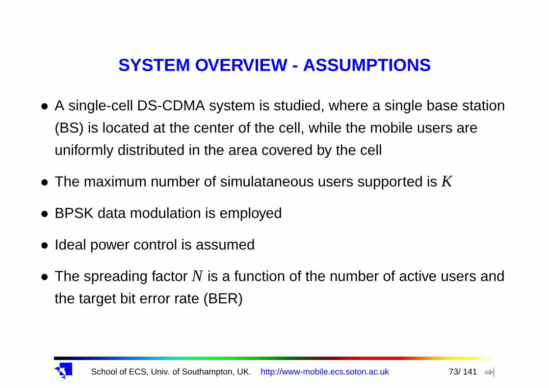
SYSTEM OVERVIEW - ASSUMPTIONS

• A single-cell DS-CDMA system is studied, where a single base station

(BS) is located at the center of the cell, while the mobile users are

uniformly distributed in the area covered by the cell

• The maximum number of simulataneous users supported is K

• BPSK data modulation is employed

• Ideal power control is assumed

• The spreading factor N is a function of the number of active users and

the target bit error rate (BER)


SYSTEM OVERVIEW - ASSUMPTIONS

• The number of interfering users, Kl can be modelled with the aid of a

Markov chain having K states

...... ......k0

(K −1)µ∆t

1− (K −1)µ∆tλ∆tλ∆tλ∆tλ∆t

µ∆t (k +1)µ∆tkµ∆t

1−λ∆t

1− (λ+ kµ)∆t

k +1k−1 K −1

• It represents a M/M/m/m queueing system, where

• λ: Arrival rate;

• 1/µ: Average service time.


K=64, =0.35, =0.009, k=k

0 500 1000 1500 2000 2500 3000Normalized time slots, n

0

10

20

30

40

50

60

Num

ber

ofac

tive

inte

rfer

ing

user

s,k

Figure 32: Markov characteristics of the number of active interfering users over the time slot interval of [0,

3000], where K is the maximum number of users.


K=64, =0.35, =0.009, k=k

1000 1200 1400 1600 1800 2000Normalized time slots, n

0

10

20

30

40

50

60

Num

ber

ofac

tive

inte

rfer

ing

user

s,k

Figure 33: Markov characteristics of the number of active interfering users over the time slot interval of [1000,

2000].


Based on the results of Fig.32 and Fig.33, we observe that

• the number of active interfering users is a slowly time-variant variable,

• it fluctuates as a function of the normalized time slot index.


c=0 dB

N=8,16,24,40,56,80,112,120

0 10 20 30 40 50 60Number of active users, Kl+1

10-5

10-4

10-3

10-2

10-1

100

BE

R,P

e

Figure 34: BER performance versus the number of active users for the parameters of γc = 0dB and spreading

factors of N = 8,16,24,40,56,80,112,120.


WHY VSF-BASED ADAPTIVE RATE TRANSMISSION

Based on the results of Fig.32, Fig.33 and Fig.34, we have the following

conclusions:

• An appropriate spreading factor can be employed within a specific time

slot for maximizing the number of bits transmitted in this specific time

slot, while maintaining the required constant target BER performance

• When the number of active users dynamically fluctuates, variable

spreading factors (VSF) can be employed by the DS-CDMA system for

achieving the maximum throughput, while guaranteeing the required

BER performance.


VSF-BASED ADAPTIVE RATE TRANSMISSIONS INDS-CDMA SYSTEMS - PRINCIPLE

The transmission rate is adapted in response to the multiuser interference

(MUI) level

• the mobile users increase their transmission rates by employing lower

spreading factors, when the number of active interfering users

decreases;

• By contrast, the mobile users decrease their transmission rates by

employing higher spreading factors, in response to an increased

number of active interfering users.


VSF-BASED ADAPTIVE RATE TRANSMISSIONS INDS-CDMA SYSTEMS - ADVANTAGES

• The rate adaption of each active user may be controlled independently;

• The adaptive-rate transmission scheme imposes no extra interference

on the system. An active user’s interference environment is affected

only by the number of active users corresponding to a certain level of

MUI, but not by their individual transmission rates;

• For DS-CDMA systems, where some active users may communicate at

constant rates, the BER and throughput of the active users

communicating at constant rates is not affected by those

communicating using adaptive rate transmissions.


K=64, k=k , PE=0.01

Adaptive

non-adaptive

=0.4 =0.006

=0.35 =0.009=0.2 =0.01

-15.0 -12.5 -10.0 -7.5 -5.0 -2.5 0.0 2.5 5.0SNR/chip, c (dB)

0.1

0.2

0.3

0.4

0.5

0.6

0.7

Thr

ough

put,

bits

/chi

p

Figure 35: Throughput performance comparison of the constant spreading factor assisted non-adaptive DS-

CDMA scheme and the VSF-assisted adaptive DS-CDMA arrangement.


K=64, k=k , PE=0.01

Adaptive

non-adaptive

=0.4 =0.006

=0.35 =0.009=0.2 =0.01

-15.0 -12.5 -10.0 -7.5 -5.0 -2.5 0.0 2.5 5.0SNR/chip, c (dB)

10-3

2

5

10-2

2

5

10-1

BE

R

Figure 36: BER performance comparison between the constant spreading factor assisted non-adaptive DS-

CDMA and the VSF-assisted adaptive DS-CDMA schemes, when they achieve the effective throughputs of Fig.35.


CONCLUSIONS

• By employing VSF-assisted adaptive rate transmissions, the effective

throughput of a DS-CDMA system may be increased by 40% upon

exploiting the Markovian distributed number of active users in the

system.

• The increased effective throughput is achieved:

– without wasting power

– without imposing extra interference upon other users

– without increasing the bit error rate (BER).


Further applications of multiple

antennas in wireless communications

• Beamforming

• SDMA

• SDM

• STTC and STBC


Beamforming [7] Typically λ/2-spaced antenna elements are used for the sake of creating a spa-

tially selective transmitter/receiver beam. Smart antennas using beamforming

have been employed for mitigating the effects of co-channel interfering signals

and for providing beamforming gain.

Spatial Diversity [5] and

Space-Time Spreading

(STBC and STTC)

In contrast to the λ/2-spaced phased array elements, in spatial diversity

schemes, such as space-time block or trellis codes [5] the multiple antennas are

positioned as far apart as possible, so that the transmitted signals of the different

antennas experience independent fading, resulting in the maximum achievable

diversity gain.

Space Division Multiple

Access (SDMA)

SDMA exploits the unique, user-specific ”spatial signature” of the individual users

for differentiating amongst them. This allows the system to support multiple users

within the same frequency band and/or time slot.

Space Division Multiplex-

ing (SDM) [Foschini 1996]

MIMO systems also employ multiple antennas, but in contrast to SDMA arrange-

ments, not for the sake of supporting multiple users. Instead, they aim for increas-

ing the throughput of a wireless system in terms of the number of bits per symbol

that can be transmitted by a given user in a given bandwidth at a given integrity.

Table 2: Applications of multiple antennas in wireless communications:The four MIMOs


Capacity of MIMO SystemsDiscrete-Input Continuous-Output Memoryless Channel (DCMC)

❏ The Full-multiplexing-gain sys-

tem has a higher asymptotic ca-

pacity as a benefit of its multi-

plexing gain.

❏ The gap between the capacity

curves of the Rayleigh fading

channel and the AWGN channel

is narrower for the full-diversity

system as a benefit of its diver-

sity gain.

ray-capacity-mimo-16qam-3.gle

-10 0 10 20 30SNR (dB)

0

1

2

3

4

5

6

7

8

9

10

11

C(b

it/sy

mbo

l)..........

.........

......

..................

......

..........

......................

......................

.........

......

......

......

........

...................

.....

...............

......

........................

....................................

....................

........

......

......

.......

.......

...........................

Nt = Nr = 2

. Multiplexing

RayleighAWGN

16-QAM, D=4

16-QAM, D=2

16-QAM, D=4

16-QAM, D=2

Diversity

The capacity of D = 2 and 4 dimensional 16QAM-based

MIMO DCMC uncorrelated Rayleigh-fading channel and

AWGN channel.


Space-Time Processing

Detection methods

Space-Time Processing Applications

Point-to-Point Point-to-Multipoint

BLAST/SDM STC

UplinkDownlink

D-BLAST SDMD

SDMABeamforming

MUD


Spatial Division Multiplexing Detection Techniques.

SDMD/MUD

Linear Detection Non-Linear Detection

LS MMSE ML SIC GA-MMSE OHRSA-ML

Log-MAP OHRSA-Log-MAP SOPHIE

• Various Space Division Multiplexing (SDM) detection methods have been studied in the context of

BLAST-type systems and their achievable performances have been evaluated using extensive computer

simulations.


Genetic Algorithm Assisted Minimum Bit Error Rate

Multiuser Detection in Multiple Antenna Aided OFDM

M. Y. Alias, S. Chen and L. Hanzo

VTC Fall, LA, USA, September 26-29, 2004

School of Electronics and Computer Science,


Tel: +44 23 8059 3125, Fax: +44 23 8059 4508

Email: {mya00r, sqc, lh}@ecs.soton.ac.uk



OUTLINE

❏ Introduction

❏ References

❏ Motivation

❏ System Model: SDMA

❏ System Model: Exact MBER Multiuser Detection

❏ System Model: Genetic Algorithm

❏ Simulation results

❏ Complexity comparison

❏ Conclusions


INTRODUCTION

❏ In an effort to increase the achievable system capacity of an OFDM system,

antenna arrays can be employed for supporting multiple users in a Space

Division Multiple Access (SDMA) communications scenario.

❏ A variety of linear multiuser detectors have been proposed for performing

the separation of OFDM users based on their unique, user-specific, spatial

signature provided that their channel impulse response was accurately esti-

mated.

❏ The most popular design strategy is constituted by the low-complexity mini-

mum mean-squared-error (MMSE) multiuser detector (MUD).


REFERENCES

1. P. Vandenameele, L. Van Der Perre, M. G. E. Engels, B. Gyselinckx, and H. J. De Man, “A

Combined OFDM/SDMA Approach,” IEEE Journals of Selected Areas in Communications, vol.

18, no. 11, pp. 2312–2321, November 2000.

2. L. Hanzo, M. Munster, B. J. Choi and T. Keller, OFDM and MC-CDMA, John Wiley and IEEE

Press, West Sussex, England, 2003.

3. B. Mulgrew and S. Chen, “Adaptive Minimum-BER Decision Feedback Equalizers for Binary

Signalling,” EURASIP Signal Processing Journal, vol. 81, no. 7, pp. 1479–1489, 2001.

4. C.-C. Yeh and J. R. Barry, “Adaptive Minimum Bit-Error Rate Equalization for Binary Signalling,”

IEEE Transactions on Communications, vol. 48, no. 7, pp. 1226–1235, July 2000.

5. M. Y. Alias, A. K. Samingan, S. Chen, and L. Hanzo, “Multiple Antenna Aided OFDM Employing

Minimum Bit Error Rate Multiuser Detection,” IEE Electronics Letters, vol. 39, no. 24, pp. 1769–

1770, 27 November 2003.

6. D. E. Goldberg, Genetic Algorithms in Search, Optimization, and Machine Learning, Addison-

Wesley, Reading, Massachusetts, 1989.


MOTIVATION

❏ However, as recognised in the literature, a better strategy is to choose the linear detec-

tor’s coefficients so as to directly minimise the error-probability or bit-error rate (BER),

rather than the mean-squared error (MSE).

❏ This is because minimising the MSE does not necessarily guarantee that the BER of

the system is also minimised. The family of detectors that directly minimises the BER

is referred to as the minimum bit-error rate (MBER) detector.

❏ In [5] we have derived the exact MBER MUD weight calculation for the uplink SDMA

OFDM system, and shown that the MBER MUD may significantly outperform the

MMSE MUD in terms of the achievable BER in a two-user OFDM scenario

❏ In this contribution, we will investigate the performance of the proposed MBER MUD

with the assistance of genetic algorithm for finding the MUD’s weight vectors, as an

alternative to the simplified conjugate gradient (CG) algorithm of [5].


SYSTEM MODEL: SDMA

User L Modulator

bL

User 22b

User 1 Modulator1b

+

n

x P

P

1n

+x 1

+x

n 2

2Modulator

Channel

Mul

tiuse

r D

etec

tor

s

1H

H 2H P

H 2H P

H 2

H

s

^

^1

2

Ls

s1

1

1

2

2

1H

2

H 1L

L

LP

2

1

sL Lb

2b

1bs

^

^

^

Figure 37: Schematic of an antenna array aided OFDM uplink scenario,

where each of the L users is equipped with a single transmit antenna and

the BS’s receiver is assisted by a P-element antenna front-end.


SYSTEM MODEL: SDMA (CONT’D)

❏ The set of complex signals received by the P-element antenna array can be

represented as:

x = Hs+n = x+n, (4)

where the received signals x, the transmitted signals s and the array noise

vector n, respectively, are given by:

x = (x1,x2, . . . ,xP)T , (5)

s = (s1,s2, . . . ,sL)T , (6)

n = (n1,n2, . . . ,nP)T , (7)

and x represents the noiseless component of x. The frequency domain chan-

nel transfer function matrix H of dimension P×L is constituted by the set of

channel transfer function vectors of the L users.


SYSTEM MODEL: SDMA (CONT’D)

❏ For linear multiuser detectors, the estimate s of the transmitted signal vector

s of the L simultaneous users is generated by linearly combining the signals

received by the P different antenna elements at the BS with the aid of the array

weight matrix W, resulting in:

s = WHx. (8)

❏ At the current state-of-the-art, the most popular MUD strategy is the MMSE

design, where wl is chosen as the unique vector minimising the MSE ex-

pressed as MSE = E[(sl − sl)2], namely as:

wl(MMSE) = (HHH +2σ2nI)−1Hl , (9)

where Hl is the l-th column of the system matrix H.


MSE and BER Surface

Error surfaces at the receiver’s

output calculated for five BPSK

modulated sources having

equal received power and

communicating over AWGN

channels at SNR=10 dB.-2-1.5

-1-0.5

0 0.5

1 1.5

2

Re{w1}

-2-1.5-1-0.5 0 0.5 1 1.5 2

Re{w2}

0 2 4 6 8

10 12 14

MSE

-0.5 0 0.5

1 1.5

2 2.5

Re{w1}

-0.5 0

0.5 1

1.5 2

2.5

Re{w2}

-6

-5

-4

-3

-2

-1

0

log10(BER)

The imaginary part of both weights of the 2-element array was fixed.


SYSTEM MODEL:EXACT MBER MULTIUSER DETECTION

Figure 38: An example of the complex, irregular shape BER

cost function of a 2-user SDMA/OFDM system supported by two

receiver antennas.

❏ The MBER solution is defined as:

wl(MBER) = argminwl

PE(wl). (10)

❏ However, the complex, irregular

shape of the BER cost function pre-

vents us from deriving a closed-form

solution for the MBER MUD weights.


SYSTEM MODEL:EXACT MBER MULTIUSER DETECTION (CONT’D)

❏ Therefore in practice an iterative strategy based on the steepest-descent gradient

method can be used for finding the weights of the MBER solution.

❏ According to this method, the linear MUD’s weight vector wl is iteratively updated,

commencing for example from the MMSE weights, until the weight vector that ex-

hibits the lowest BER is arrived at.

❏ In each step, the weight vector is updated according to a specific step-size, µ,

in the vectorial direction in which the BER cost function decreases most rapidly,

namely in the direction opposite to the gradient of the BER cost function.


SYSTEM MODEL: GAUse the probability of error

functionequation as the objective

Start GA

Is terminationcriterion met?

Initialisation

Evaluation

No

Evaluation

Mutation

Crossover

Selection Decisiontaken

Finish GA

Convert binary string to weightvalues

Yes

Figure 39: Flowchart of the BER optimisation using a

GA.

❏ Even though the MBER detector of [5] is ca-

pable of maintaining a good performance, the

convergence of the algorithm is sensitive to

the choice of the algorithm’s parameters.

❏ An attractive method that might be able to

assist the MBER MUD in circumventing the

above-mentioned problems is constituted by

the family of genetic algorithms (GA) [6].

❏ GAs may be invoked in robust global search

and optimisation procedures that do not re-

quire the knowledge of the objective function’s

derivatives or any gradient-related information

concerning the search space.


SIMULATION RESULTSParameter Value or type

SDMA 4 users and 4 receiver antennas

OFDM 128 subcarriers and 32 cyclic prefix

GA

Population size 30

Number of generations 100

Probability of mutation 0.01

Crossover type Single-point crossover

Probability of crossover 0.6

Genome type Binary string

Encoding/decoding Binary encoding and decoding

Channel impulse response h(z) = 0.8854+0.3504z−6

+0.2881−11, dispersive Gaussian channel [2]

Table 3: Parameters for the GA simulations.


SIMULATION RESULTS (CONT’D)

0 5 10 15 20 25 30 35 40Average SNR (dB)

10-7

10-6

10-5

10-4

10-3

10-2

10-1

100

Ave

rage

BE

R

1-user 1-antenna AWGNGA MBER DetectorCG MBER DetectorMMSE Detector

Figure 40: The average BER performance of the four

different users characterised in an SDMA system employ-

ing four receiver antennas and 128-subcarrier OFDM for

communicating over the OFDM symbol-invariant disper-

sive Gaussian channel given in Table 3.

❏ The parameters used for our simulations are

outlined in Table 3.

❏ A dispersive Gaussian channel was used,

where the z-domain transfer function associ-

ated with the CIR is given by h(z) = 0.8854+

0.3504z−6 +0.2881z−11 [2].

❏ As a starting point, we used binary type

genomes [6] for representing the GA’s individ-

uals. The GA’s termination criterion is consti-

tuted by the maximum affordable number of

generations.


COMPLEXITY COMPARISON

010-7

10-6

10-5

10-4

10-3

10-2

10-1

4000 8000 12000 16000 20000Complexity

-7

-6

-5

-4

-3

-2

-1L

og10

(Ave

rage

BE

R)

MMSE MUDGA MBERCG MBER

Figure 41: The BER performance of User 1 versus

complexity for the GA and CG MBER MUD invoked in

the OFDM/SDMA system employing P = 4, L = 4 and

128-subcarrier OFDM for communicating over the symbol-

invariant dispersive Gaussian channel given in Table 3 at

SNR = 15 dB.

❏ The complexity of the CG algorithm is proportional to the

number of iterations used for finding the MBER solution on

the BER surface.

Compl{CG} ' Max. number of iter. (11)

❏ If we used the maximum number of generations as the ter-

mination criterion in the GA, each generation of the popu-

lation contains a certain number of individuals, thus

Compl{GA} ' Pop. size×Gen. (12)


CONCLUSIONS

❏ In this contribution, we have shown that GAs may be applied in the context of an SDMA

OFDM system for determining the MBER MUD’s weight vectors.

❏ The GA-aided system has an edge over the CG-based system, because it does not

require an initial weight solution.

❏ It was also shown that the GA is capable of approaching the MBER solution at a lower

complexity than the CG algorithm.

❏ Our future work will invoke forward error correction codes in high-dimensional SDMA-

MUDs.


Reduced-Complexity Maximum-Likelihood SDMSphere-Detector for Rank-Deficient Scenarios

1

0

2

0.17

3

0.34

4

0.52

5

0.69

6

0.86

7

1.04

8

1.21

9

1.38

10

1.56

11

1.73

12

1.91

13

2.08

14

2.25

15

2.43

16

2.6

0

139


Reduced-Complexity SDM Sphere-Detector for Rank-Deficient Scenarios

10-6

10-5

10-4

10-3

10-2

10-1

100

0 5 10 15 20

BE

R

Eb/N0 [dB]

sdm-cmp-16qam : 27-Jun-2005

SOPHIEMMSE

mt=6,nr= 16QAM 464QAM 6

• The proposed SOPHIE SDM detection method exhibits near-optimum performance and relatively low

complexity in high-throughput scenarious such as 6x6 64QAM as well as rank-deficient 6x4 16QAM

MIMO-OFDM. The throughout is 36 and 24 bits/symbol, respectively.


Iterative Joint Receiver Architecture.

Channel

Estimator

Space-Time

DetectorDecoder 1 Decoder 2y

y

H

c d

turbo decoder

joint detector-decoder

extr. info.

extr. info.

extr. info.

• A joint data detection and channel estimation based turbo architecture is developed, where a succession of

detection modules constituting a MIMO-OFDM receiver iteratively exchange soft information, thus resulting

in a substantial system performance improvement.


Joint Iterative MIMO-OFDM Receiver

…

…

…

User 1

GA-aided

Iterative Joint

Channel

Estimator and

Multi-User

Detector

IFFT

SDMA MIMO Channel

(1)sb

1x

2x

Px

User 1

User 2

FFT

FFT

Base Station (BS)

Mod.

Geographically-separated Mobile Stations (MSs) …

…

…

…

…

User 2 IFFT

IFFT

Mod.

Mod. User L

…

…

…

User L FFT

P-element

Receiver

Antenna

Array

FEC Encoder

FEC Decoder

FEC Decoder

FEC Decoder

FEC Encoder

FEC Encoder

(2)b

( )Lb

(1)b

(1)b

(2)b

( )ˆ Lb

(1)s

(2)s

( )Ls

(2)sb

( )Lsb

(1)ˆsb

(2)ˆsb

( )ˆ Lsb


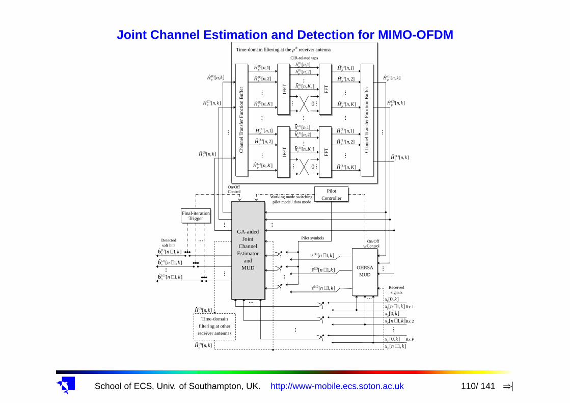
Joint Channel Estimation and Detection for MIMO-OFDM

…

…

…

Final-iteration Trigger

…

IFF

T

Cha

nnel

Tra

nsfe

r F

unct

ion

Buf

fer

GA-aided Joint

Channel Estimator

and MUD

OHRSA

MUD

( )ˆ [ , ]lpH n k

(2)[ , ]pH n k

�

(1)[ , ]pH n k

�

…

(1)[ , ]pH n K

�

(1)[ ,2]pH n

�

(1)[ ,1]pH n

�

…

…

(1)0[ , ]ph n K

�

(1)[ ,2]ph n

�

(1)[ ,1]ph n

�

…

FFT

…

…

0

…

(1)ˆ [ , ]pH n K

(1)ˆ [ ,2]pH n

(1)ˆ [ ,1]pH n

Cha

nnel

Tra

nsfe

r F

unct

ion

Buf

fer

IFF

T

…

( )[ ,2]LpH n

�

( )[ ,1]LpH n

…

( )0[ , ]L

ph n K

( )[ ,2]Lph n

�

( )[ ,1]Lph n

�

FFT

…

…

0

…

( )ˆ [ , ]LpH n K

( )ˆ [ ,2]LpH n

( )ˆ [ ,1]LpH n

…

Pilot

Controller

( )ˆ [ , ]LpH n k

(2)ˆ [ , ]pH n k

(1)ˆ [ , ]pH n k

…

…

Pilot symbols

(1)[ 1, ]s n k+

… …

…

(1)ˆ [ 1, ]s n k+b

(2)ˆ [ 1, ]s n k+b

( )ˆ [ 1, ]Ls n k+b

Time-domain filtering at the pth receiver antenna

Time-domain

filtering at other

receiver antennas

( )[ , ]lpH n k

�

( )ˆ [ , ]lpH n k

Detected soft bits

…

CIR-related taps

On/Off Control

…

…

On/Off Control

( )[ , ]LpH n K

�

1[0, ]x k

1[ 1, ]x n k+

2[0, ]x k

2[ 1, ]x n k+

[0, ]Px k[ 1, ]Px n k+

Working mode switching: pilot mode / data mode

Rx 1

Rx 2

Rx P

(2)[ 1, ]s n k+�

( )[ 1, ]Ls n k+� Received signals

…


Joint Channel Estimation and Detection for MIMO-OFDM

-2.0 -1.5 -1.0 -0.5 0.0 0.5 1.0 1.5 2.0Real

-2.0

-1.5

-1.0

-0.5

0.0

0.5

1.0

1.5

2.0Im

agin

ary

True Channel Transfer Functions, 2-path Rayleigh

...................

.......

. . . . . . . . . . . . . . . . . . . . . . .................................

........

. .. . . . . . . . . . . . . . . . . . . . . ....

.

..............................

..

....

. .. . . . . . . . . . . . . . . . . . . . .................................

..........

. . . . . . . . . . . . . . . . . . . . . ...................................

....... .

. . . . . . . . . . . . . . . . . . . . . ...................................

....... .

. . . . . . . . . . . . . . . . . . . . . ...................................

..

..... .

. . . . . . . . . . . . . . . . . . . . ...................................

........

. . . . . . . . . . . . . . . . . . . . . ...................................

........

. . . . . . . . . . . . . . . . . . . . . ...................................

........

. . . . . . . . . . . . . . . . . . . . . ...................................

........

. . . . . . . . . . . . . . . . . . . . ...................................

........

. . . . . . . . . . . . . . . . . . . . . ...................................

........

. . . . . . . . . . . . . . . . . . . . . ...................................

........

. . . . . . . . . . . . . . . . . . . . . ..................................

........

. .. . . . . . . . . . . . . . . . . . . .................................

..........

. .. . . . . . . . . . . . . . . . . . . .................................

..........

. .. . . . . . . . . . . . . . . . . . . .................................

..........

. .. . . . . . . . . . . . . . . . . . . ................................

............

. . . . . . . . . . . . . . . . . . . ...................................

........

. .. . . . . . . . . . . . . . . . . . . .................................

..........

. .. . . . . . . . . . . . . . . . . . . ................................

....

..

......

. . . . . . . . . . . . . . . . . . . ...................................

..........

. . . . . . . . . . . . . . . . . . . ...................................

..........

. . . . . . . . . . . . . . . . . . . ..................................

..........

. .. . . . . . . . . . . . . . . . . . ................................

....

..

......

. . . . . . . . . . . . . . . . . . . ...................................

..........

. . . . . . . . . . . . . . . . . . . ...................................

..........

. . . . . . . . . . . . . . . . . . . ..................................

..........

. .. . . . . . . . . . . . . . . . . .................................

....

..

......

. .. . . . . . . . . . . . . . . . . .................................

............

. .. . . . . . . . . . . . . . . . . ................................

....

........

. .. . . . . . . . . . . . . . . . . .................................

....

........

. .. . . . . . . . . . . . . . . . . .................................

....

..

......

. .. . . . . . . . . . . . . . . . . ................................

....

..........

. . . . . . . . . . . . . . . . . . ..................................

..........

. .. . . . . . . . . . . . . . . . . .................................

....

........

. .. . . . . . . . . . . . . . . . . ................................

....

..........

. . . . . . . . . . . . . . . . . . ..................................

............

. . . . . . . . . . . . . . . . . ...................................

..........

... . . . . . . . . . . . . . . . . ...........................

No. of OFDM symbols=40FD=0.003

User 1

User 2

User 3

User 4


-2.0 -1.5 -1.0 -0.5 0.0 0.5 1.0 1.5 2.0Real

-2.0

-1.5

-1.0

-0.5

0.0

0.5

1.0

1.5

2.0

Imag

inar

y

Estimated Channel Transfer Functions, 2-path Rayleigh

..

.

..

. .

... .

.

.

.

..

...

. ..

...

..

.... . ..

...

..

. . . ...

. ... .

..

.. .

..

. ..

..

.

.

..... ....

. ....

...

.

.

.. .

. . ...

.. . . . . . . . . . . .

.. ..

.. . ... .

. ...

.....

.... .

............

.....

.. .

. ...

. ....

.. ... . . . . .. . . .

.

.. .. ..

...

....

.

.....

........

........

....

.

..

....

. ..

. . ..

.

.. . .. . .

.. .

. .. . .

..

. .... .

.....

.. ...

....

..

......

.....

....

.

....

. . ... .. .

. . .. .. . . .

...

...

.....

..........

...........

. ..

.. .

.....

.. .

... .. .

. .. .

.. .... .

....

. ... .

....

..................

...

.

.

.

..

. ..

. . ... . ..

.... .

...

. . . . . ..

...

. .

..

.....

... .......

........

...

.

..

... ..

.. .... .. .

. . ..

. ..... . .

......

. .. .....

.................

....

. .

..... ..

.. . .

....

.. . . . ...

. . . . . .

...

..... ..

.

..

.. .........

..... .....

...

.. . .

.. . . ... . ..

... . . . .. . .

. .. .

.

.. .. .

.......

..........

..........

....

. ... .

.... .

.

.. .

. .. . .

. ..

.

. ... .

......

....

...

.. ...

.... ........

..

....... ..

... ..

. .. . . .

... ..

..

. . ....

....

.......

..

........

.....

.....

..

....... . .

..

.. . ..

. . . . . .. ..

.. .

.. .

.....

.... ...

....

.......

.....

..

..... .....

.. . .. .. . . . .. .. . .. .

. .. .

....

.......

... ....

..........

... ..

...

..... .. .

. .. .. . . .. . .

.. ... ...

..

..

. .......

............

..

.. ...

..

.. .

. .. .. .. .

... . . .

. ...

.. .

. .. .

..

....

..

......

...............

.. ....

.... .

....

.... . . . .

...

.. . ..

. ... ..

.

...

.... ....

.............

...

......

...

.... ...

.... . .

.. . . .

..

. . ... .

. . .

. ...

...

.. ..

.. ........

. .....

.. .....

. ..

...

. . .. .

. . .. ..

.. .. .

. ... ....

..

. .....

......

.....

......

....

. . .. ....

.

. .

. .. . .. .

. ..

. ..

.. .

...

..

......

...... .

...

.............

....

....

......

... . .

. . ... .. .. . . .

.....

...

.. .

..

......

........

.......

. ...

.. .....

.. .. .

. .

.. . . .. . . .

..

. ..

............

.........

... .. ..

........ ...

.. ..

. .. .... .

.. . ..

.. .. . .

. .........

..

......

....... ....

.. ....

....

.. ... ..

... . . . . . .

.. . . ..

.. . . .

..

.. ... .

......

.....

......

...

.......

. .. ... ..

.

... . .. . . . . .. .. .. .. .. ...

..

.......

.....

............

. ...

.

.... .

....

....

.

. . .. . ....

. . ...

. ... .

..

.....

......

.........

.....

... .

.. ....

.... ..

. . . .. . .. . ..

. ....... . ...

.....

.

.....

...

........

......

...... .

.. ..... .

.. .... . .

... ... . . . ....

....... ..

.

. ...

.. ..........

. ...

...... ....

. . . . . .. .. . .. . .. .

.. .. .

....

..... .

..........

......

.. ....

.......

.... .

..

.. . ... . . ..

. .. .. .

.. ....

....

.... .....

.... .

. ....

.....

. .. . ..

.. .. . .

. . .. . .. . .. . .. .. .

... ... ..

............

.. ......

.

....

.... .... ..

....

. . . . . .. .. . .. .

. .... .. ....

.. ..... ..

..... ........

...

..

...

... ..

.... . ....

...

..

.. . . .

. . .... .

..

.. .....

... ...

...

... ..

. .....

...

..

...

.. ....

.. . . . . .. .... ..

.. .. .

.. ..... ..

.. .

...........

....

....

...

... . .

. .. . . ..

. . . . . . .. .....

. . ... ....

.....

. .

...

.. ......

........

... ..

.

.

... . .. . .. . ..

. . . .. .. ..

.. . ..

.........

.....

. .... ..........

..

...

..

.....

. ..... .

.... . .

.. .. ...

... ..

.. ......

........

..... ...

.....

.........

.

.. ..

. .

.

. . . . . ... .. .. .

....

.. ... ....

......

............

...

... .

. ...

..... ..

. . ... .. . . . ... ..

.. ... .

... ......... .....

.....

.. ..... .

....

.... . ..

...

...

. .. .. . .. .. .

. .

. .......

..........

.....

No. of OFDM symbols=40FD=0.003

GA. Itr.=1=2.5%

SNR=20dB

User 1

User 2

User 3

User 4


GA-JCEMUD Performance

fdx_u4r2_jga_ldpc_4qam_mul.gle Mon Oct 10 2005 19:09:06

0 5 10 15 20 25 30SNR (dB)

10-5

10-4

10-3

10-2

10-1

100

BE

R

LDPC-GA-JCEMUD-SDMA-OFDM, L4/P2, 4QAM, 2-path Rayleigh

GA-JCEMUD, FD=0.005GA-JCEMUD, FD=0.003GA-JCEMUD, FD=0.001MMSE, Perfect CSIML, Perfect CSI

=2.5%GA. Itr.=1

LDPC-codedUncoded


GA-JCEMUD Performance

mse_fft-itx_u4r2_jga_ldpc_4qam_mul.gle Sat Sep 10 2005 14:26:24

0 5 10 15 20 25 30SNR (dB)

10-3

2

5

10-2

2

5

10-1

2

5

100

Cha

nnel

MSE

GA-JCEMUD-SDMA-OFDM, L4/P2, 4QAM, 2-path Rayleigh

GA. Itr.=2, =2.5%GA. Itr.=2, =100%GA. Itr.=1, =2.5%GA. Itr.=1, =100%GA. Itr.=0, =2.5%GA. Itr.=0, =100%FD=0.003

SchoolofE

CS

,Univ.

ofSoutham

pton,UK

.http://w

ww

-mobile.ecs.soton.ac.uk

115/141⇒|

CH

AN

NE

LVA

RIA

TIO

NIN

SPA

CE

-TIM

EC

OD

ED

OF

DM

1T

x1

Rx

0128

256384

512

Subcarrierindex0

2550

75100

125150

Transm

issionfram

e(T

ime)

4 5 6 7 8 9 10 11

12 13 14

Instantenous SNR (dB)2

Tx

1R

x

0128

256384

512

Subcarrierindex0

2550

75100

125150

Transm

issionfram

e(T

ime)

4 5 6 7 8 9 10 11

12 13 14

Instantaneous SNR (dB)

2T

x2

Rx

0128

256384

512

Subcarrierindex0

2550

75100

125150

Transm

issionfram

e(T

ime)

4 5 6 7 8 9 10 11

12 13 14


2T

x6

Rx

0128

256384

512

Subcarrierindex0

2550

75100

125150

Transm

issionfram

e(T

ime)

4 5 6 7 8 9 10 11

12 13 14



Effects of Rate Adaptation on the Throughput of Random

Ad Hoc Networks

Xiang Liu and Lajos Hanzo

Communications Research Group

School. of Electronics and Computer Science,




Outline

❏ The system model of wireless ad hoc networks.

❏ The achievable per-node throughput improvements of perfect rate adaptation

are investigated in the following two scenarios:

❍ Only pathloss is taken into account,

❍ Shadowing is also taken into account.

❏ Conclusions: Perfect rate adaptation has the potential of considerably improv-

ing the achievable throughput of the random ad hoc network compared to

fixed rate transmissions. However, even perfect rate control fails to change

the scaling law of the per-node throughput result given by Θ(

1√n logn

)

in [1],

regardless of the absence or presence of shadow fading.


Contributions

❏ In contrast to most of the existing literature, where a fixed transmission rate

associated with a time-invariant modulation scheme was assumed [1, 2, 3, 4,

5, 6], we consider the employment of perfect rate adaptation as well as the

effects of a fading channel

❏ Two formulas are provided for characterizing the beneficial effects of rate

adaptation on the achievable per-node throughput of random ad hoc networks

both in the absence and in the presence of shadow fading.


System Model

❏ A random ad hoc network supports n nodes uniformly and independently dis-

tributed in a unit area S , which is a planar disk as in [1].

❏ All nodes share the same bandwidth, which is given by W Hz.

❏ All packet-transmissions are slotted into perfectly synchronized time slots.

❏ No node is capable of simultaneously transmitting and receiving signals, or

simultaneously transmitting/receiving signals to/from more than one node.

❏ The minimum SINR required for successful reception is β.

❏ The common reliable transmission range rn of all nodes is chosen to guaran-

tee the asymptotic connectivity of random networks.

❏ Initially the minimum distance between nodes is assumed to be rmin, which

satisfies rmin < rn.


System Model

❏ The power of each transmitting node is fixed to Pt Watts, i.e. no power control

is used, which is typical in cost-efficient ad hoc networks.

❏ Let Nt be the subset of nodes simultaneously transmitting at some time in-

stant. If node i, i /∈ Nt is receiving signals from node j, j ∈ Nt , then the SINR

experienced at node i becomes:

γ ji =PtG ji

∑k∈Nt ,k 6= j PtGki +ηi, (13)

where γ ji is the SINR at node i experienced by the signal arriving from node j,

while Gki is the power gain between nodes k and i, and ηi is the background

noise encountered at node i.

❏ The value of the power gain G ji depends on the propagation model, which will

be discussed later, taking into account the absence of fading or the presence

of log-normal shadow fading, respectively.


Notations

❏ α is the path loss exponent in the pathloss model.

❏ σ is the standard deviation of the lognormal shadowing.

❏ cg is the average per-node throughput achievable without rate adaptation,

which is fixed and determined by the Shannon limit at the minimum required

SINR β.

❏ ca is the average per-node throughput achievable with the advent of perfect

rate adaptation.

❏ ci =ca

cgis the normalized per-node throughput improvement achievable with

the advent of perfect rate adaptation.

❏ c0i = max

rmin{ci} is the maximum achievable normalized per-node throughput

improvement ci attained with the advent of perfect rate adaptation, when we

have rmin = 0.


The Effects of Path Loss:The Normalized Per-Node Throughput Improvement ci Achievable

with the Advent of Perfect Rate Adaptation

Theorem 1

ci =2

∫ 1u s ln(1+βs−α)ds

(1−u2) ln(1+β)≤ 2

∫ 10 s ln(1+βs−α)ds

ln(1+β)

= c0i < +∞, (14)

❍ u =rmin

rnis the normalized minimum distance between ad hoc nodes,

❍ s =r ji

rnis the normalized distance.


The Effects of Path Loss:ci versus rmin/rn for different values of α

0.0 0.1 0.2 0.3 0.4 0.5 0.6 0.7 0.8 0.9 1.0Normalized minimum distance between nodes, rmin/rn

1.0

1.2

1.4

1.6

1.8

2.0

2.2

2.4

Nor

mal

ized

thro

ughp

utim

prov

emen

t,c i

=10 dB=4=3=2

Figure 42: The normalized per-node throughput improvement ci versus the normalized minimum distance

rmin/rn between nodes for different values of the path loss exponent α at a required SINR value of β = 10 dB in

the absence of fading, which is computed from Equation 14.


The Effects of Path Loss:ci versus rmin/rn for different values of β


1.0

1.5

2.0

2.5

3.0

3.5

4.0

Nor

mal

ized

thro

ughp

utim

prov

emen

t,c i

=20 dB=10 dB=0 dB=3


rmin/rn between nodes for different values of the required SINR β at a path loss exponent of α = 3 in the absence

of fading, which is computed from Equation 14.


The Effects of Path Loss:c0

i versus α for different values of β

2.0 2.2 2.4 2.6 2.8 3.0 3.2 3.4 3.6 3.8 4.0Path loss exponent,

1.0

1.5

2.0

2.5

3.0

3.5

4.0

4.5

5.0

Nor

mal

ized

thro

ughp

utim

prov

emen

tupp

erbo

und,

c i0

=20 dB=10 dB=0 dB

Figure 44: The normalized per-node throughput improvement upper bound c0i versus the pathloss exponent α

plotted for different values of the target SINR β in the absence of fading, which is evaluated from Equation 14. The

transmit power is fixed and perfect rate adaptation is assumed.


The Effects of Path Loss:c0

i versus β for different values of α

0 2 4 6 8 10 12 14 16 18 20Required SINR, (dB)

1.0

1.5

2.0

2.5

3.0

3.5

4.0

4.5

5.0

Nor

mal

ized

thro

ughp

utim

prov

emen

tupp

erbo

und,

c i0

=4=3=2

Figure 45: The normalized per-node throughput improvement upper bound c0i versus the target SINR β plotted

for different values of the pathloss exponent α in the absence of fading, which is evaluated from Equation 14. The

transmit power is fixed and perfect rate adaptation is assumed.


The Effects of Shadow Fading:The Normalized Per-Node Throughput Improvement ci Achievable

with the Advent of Perfect Rate Adaptation

Theorem 2

ci =

∫ +∞0 ln(1+βet)dt

∫ 0u e2se

− (t+αs)2

2σ2 ds

ln(1+β)∫ +∞

0 dt∫ 0

u e2se− (t+αs)2

2σ2 ds

≤∫ +∞

0 ln(1+βet)dt∫ 0−∞ e2se

− (t+αs)2

2σ2 ds

ln(1+β)∫ +∞

0 dt∫ 0−∞ e2se

− (t+αs)2

2σ2 ds

= c0i < +∞, (15)

❍ u = lnrmin− lnrn is the logarithmic normalized minimum distance between ad

hoc nodes,

❍ s = lnr ji − lnrn is the logarithmic normalized distance,

❍ t = lnγ ji − lnβ is the logarithmic normalized SINR.


The Effects of Shadow Fading:ci versus rmin/rn for different values of α


1.0

1.2

1.4

1.6

1.8

2.0

2.2

2.4

Nor

mal

ized

thro

ughp

utim

prov

emen

t,c i

=8 dB=10 dB=4=3=2


rmin/rn between nodes for different values of the path loss exponent α at a required SINR value of β = 10 dB and

a lognormal shadowing standard deviation of σ = 8 dB in the presence of shadow fading, which is computed from

Equation 15.


The Effects of Shadow Fading:ci versus rmin/rn for different values of β


1.0

1.5

2.0

2.5

3.0

3.5

4.0

Nor

mal

ized

thro

ughp

utim

prov

emen

t,c i

=8 dB=20 dB=10 dB=0 dB=3


rmin/rn between nodes for different values of the required SINR β at a path loss exponent value of α = 3 and a

lognormal shadowing standard deviation of σ = 8 dB in the presence of shadow fading, which is computed from

Equation 15.


The Effects of Shadow Fading:ci versus rmin/rn for different values of σ


1.0

1.2

1.4

1.6

1.8

2.0

2.2

2.4

Nor

mal

ized

thro

ughp

utim

prov

emen

t,c i

=12 dB=8 dB=5 dB=10 dB=3


rmin/rn between nodes for different values of the lognormal shadowing standard deviation σ at a path loss expo-

nent value of α = 3 and a required SINR of β = 10 dB in the presence of shadow fading, which is computed from

Equation 15.


The Effects of Shadow Fading:c0

i versus α for different values of β


1.0

1.5

2.0

2.5

3.0

3.5

4.0

4.5

5.0

Nor

mal

ized

thro

ughp

utim

prov

emen

tupp

erbo

und,

c i0

=8 dB=20 dB=10 dB=0 dB

Figure 49: The normalized per-node throughput improvement upper bound c0i versus the pathloss exponent α

plotted for different values of the target SINR β at a lognormal shadowing standard deviation of σ = 8 dB in the

presence of shadow fading, which is evaluated from Equation 15. The transmit power is fixed and perfect rate

adaptation is assumed.



i versus α for different values of σ


1.0

1.5

2.0

2.5

3.0

3.5

4.0

4.5

5.0

Nor

mal

ized

thro

ughp

utim

prov

emen

tupp

erbo

und,

c i0

=12 dB=8 dB=5 dB=10 dB

Figure 50: The normalized per-node throughput improvement upper bound c0i versus the pathloss exponent

α plotted for different values of the lognormal shadowing standard deviation σ at a target SINR of β = 10 dB in

the presence of shadow fading, which is evaluated from Equation 15. The transmit power is fixed and perfect rate




i versus β for different values of α

0 2 4 6 8 10 12 14 16 18 20Required SINR, (dB)

1.0

1.5

2.0

2.5

3.0

3.5

4.0

4.5

5.0

Nor

mal

ized

thro

ughp

utim

prov

emen

tupp

erbo

und,

c i0

=8 dB=4=3=2


for different values of the pathloss exponent α at a lognormal shadowing standard deviation of σ = 8 dB in the





i versus β for different values of σ

0 2 4 6 8 10 12 14 16 18 20Required SINR, (dB)

1.0

1.5

2.0

2.5

3.0

3.5

4.0

4.5

5.0

Nor

mal

ized

thro

ughp

utim

prov

emen

tupp

erbo

und,

c i0

=12 dB=8 dB=5 dB=3


for different values of the lognormal shadowing standard deviation σ at a pathloss exponent of α = 3 in the





i versus σ for different values of α

5 6 7 8 9 10 11 12Lognormal shadowing standard deviation, (dB)

1.0

1.5

2.0

2.5

3.0

3.5

4.0

4.5

5.0

Nor

mal

ized

thro

ughp

utim

prov

emen

tupp

erbo

und,

c i0

=10 dB=4 dB=3 dB=2 dB

Figure 53: The normalized per-node throughput improvement upper bound c0i versus the lognormal shadowing

standard deviation σ plotted for different values of the pathloss exponent α at a target SINR of β = 10 dB in the





i versus σ for different values of β

5 6 7 8 9 10 11 12Lognormal shadowing standard deviation, (dB)

1.0

1.5

2.0

2.5

3.0

3.5

4.0

4.5

5.0

Nor

mal

ized

thro

ughp

utim

prov

emen

tupp

erbo

und,

c i0

=20 dB=10 dB=0 dB=3

Figure 54: The normalized per-node throughput improvement upper bound c0i versus the lognormal shadowing

standard deviation σ plotted for different values of the target SINR β at a pathloss exponent of α = 3 in the




Example: AQAM Parameters

k 0 1 2 3 4 5 6

Mk 0 2 4 16 64 256 1024

bk 0 1 2 4 6 8 10

sk(dB) BER = 10−3 −∞ 6.7895 9.7998 16.5430 22.5490 28.4147 34.2607

sk(dB) BER = 10−5 −∞ 9.5879 12.5982 19.4551 25.5684 31.5341 37.4728

mode No Tx BPSK QPSK 16-QAM 64-QAM 256-QAM 1024-QAM

Table 4: The parameters of K-mode square AQAM systems using Gray coding and designed for maintaining

BER = 10−3 and 10−5, respectively. The switching thresholds were evaluated from Equations 14, 16 in [7] and

γ = γs/ log2 M.

❍ K is the number of modulation modes used in the AQAM scheme.

❍ Mk is the constellation size in the kth mode.

❍ bk is the number of bits per symbol (BPS) transmitted in the kth mode.

❍ sk is the switching level between the (k−1)th and kth modes.


Example: AQAM Results

1 2 3 4 5 6Number of AQAM modes, K

0.0

0.5

1.0

1.5

2.0

2.5

3.0

3.5

4.0

Nor

mal

ized

BPS

thro

ughp

ut,B

i

K-mode AQAM, BER=10-5

, in the presence of shadowingK-mode AQAM, BER=10

-3, in the presence of shadowing

K-mode AQAM, BER=10-5

, in the absence of fadingK-mode AQAM, BER=10

-3, in the absence of fading

Figure 55: The achievable normalized per-node average BPS throughput Bi versus the number of modes K in

K-mode square AQAM systems using Gray coding for a path loss exponent value of α = 3, a lognormal shadowing

standard deviation of σ = 8 dB and a target BER of 10−3 and 10−5, respectively, recorded both in the absence of

fading and in the presence of shadow fading in a random ad hoc network.


Conclusion

❏ Perfect rate adaptation has the potential of considerably improving the achievable

throughput of the random ad hoc network compared to fixed rate transmissions,

since rate adaptation is capable of mitigating the effects of link quality fluctuations,

as shown in Figures 42 - 48.

❏ However, Theorem 1 and 2 revealed that even perfect rate control fails to change

the scaling law of the per-node throughput result given by Θ(

1√n logn

)

in [1], re-

gardless of the absence or presence of shadow fading.

❏ This conclusion was further confirmed by Figure 55 in the context of our AQAM

examples.


[1] P. Gupta and P. Kumar, “The Capacity of Wireless Networks,” IEEE Transactions on Information Theory, vol. 46,

pp. 388–404, March 2000.

[2] A. Spyropoulos and C. Raghavendra, “Capacity Bounds for Ad-Hoc Networks Using Directional Antennas,” in

IEEE International Conference on Communications, vol. 1, (Anchorage, Alaska, USA), pp. 348–352, 11-15 May

2003.

[3] A. Spyropoulos and C. Raghavendra, “Asympotic Capacity Bounds for Ad-Hoc Networks Revisited: the Direc-

tional and Smart Antenna Cases,” in IEEE Global Telecommunications Conference, vol. 3, (San Francisco, Cali-

fornia, USA), pp. 1216–1220, 1-5 December 2003.

[4] M. Grossglauser and D. Tse, “Mobility Increases the Capacity of Ad Hoc Wireless Networks,” IEEE/ACM Trans-

actions on Networking, vol. 10, pp. 477–486, August 2002.

[5] B. Liu, Z. Liu, and D. Towsley, “On the Capacity of Hybrid Wireless Networks,” in IEEE INFOCOM, vol. 2, (San

Francisco, Carlifornia, USA), pp. 1543 –1552, 30 March-3 April 2003.

[6] U. C. Kozat and L. Tassiulas, “Throughput Capacity of Random Ad Hoc Networks with Infrastructure Support,” in

International Conference on Mobile Computing and Networking, (San Diego, Carlifornia, USA), pp. 55–65, 14-19

September 2003.

[7] K. Cho and D. Yoon, “On the General BER Expression of One- and Two-Dimension Amplitude Modulations,” IEEE

Transactions on Communications, vol. 50, pp. 1074–1080, July 2002.


Thank you...

advanced wireless networking and cross-layer optimization

Documents