advanced topics in population and community ecology and ... · advanced topics in population and...
TRANSCRIPT

Advanced Topics in Population and Community Ecologyand Conservation
Lecture 1
Ana I. BentoImperial College London
MRC Centre for Outbreak Analysis and Modelling
II Southern-Summer School on Mathematical BiologyJanuary 2013
Ana I. Bento Imperial College London Advanced Topics-II Southern Summer School January 2013 1 / 41

Overview
Today we will...
Revise the concept of population
Introduce demographic concepts
Matrix population models
Ana I. Bento Imperial College London Advanced Topics-II Southern Summer School January 2013 2 / 41

Overview
Today we will...
Revise the concept of population
Introduce demographic concepts
Matrix population models
Ana I. Bento Imperial College London Advanced Topics-II Southern Summer School January 2013 2 / 41

Overview
Today we will...
Revise the concept of population
Introduce demographic concepts
Matrix population models
Ana I. Bento Imperial College London Advanced Topics-II Southern Summer School January 2013 2 / 41

A quick review
A population is...
A group of individuals of one species that can be defined as a singleunit, distinct from other such units
a cluster of individuals with a high probability of mating with eachother, compared to their probability of mating with members ofanother population
Ana I. Bento Imperial College London Advanced Topics-II Southern Summer School January 2013 3 / 41

A quick review
Fundamental equation of population change
Nt+1 = Nt + B − D + I − E
Where:
Nt = the number of organisms now
Nt+1 = the number of organisms in the next time step per year pergeneration
B = the number of births
D = the number of deaths
I = the number of immigrants
E = the number of emigrants
Ana I. Bento Imperial College London Advanced Topics-II Southern Summer School January 2013 4 / 41

A quick review
This is often simplified to
Nt+1 = λNt
Where:
λ summarises B − D + I − E
λ is the net reproductive rate - the number of organisms next year perorganism this year
dNdt = rN
Where:
r = lnN- the intrinsic rate of increase
Ana I. Bento Imperial College London Advanced Topics-II Southern Summer School January 2013 5 / 41
A quick review
Describing mortality and fecundity
Fecundity is often expressed on a per capita basis, which meansdividing the total fecundity by population size
Mortality is often expressed as a proportion or percentage dying in atime interval
If d individuals die in a population of N individuals, then s = N − dsurvive and the probability of dying, p = d
N
Easiest way to collect such data is from marked individuals
Ana I. Bento Imperial College London Advanced Topics-II Southern Summer School January 2013 6 / 41

Data collection
How to collect data that is useful
Follow individuals throughout their lives recording birth data, breedingattempt data and movement and death data
In practice it is nearly always impossible to do this. Bighorn sheep atRam Mountain offer one exception
Ana I. Bento Imperial College London Advanced Topics-II Southern Summer School January 2013 7 / 41

Data collection
What if data are not complete?
Animal seen known to be alive (1)
Animal not seen, but not dead as seen in a later census- either alivebut not seen and living in study area or temporarily emigrated (0)
Animals not seen now or in later census- either alive but not seen andliving in the study or emigrated or dead (Last two zeros)
Ana I. Bento Imperial College London Advanced Topics-II Southern Summer School January 2013 8 / 41

Analysis of capture histories to estimate survival
Mark Recapture Analysis
Mark Recapture Analysis: estimates survival probabilities fromrecapture histories by examining what the probability of sighting ananimal in a specific demographic class is, given that it has to be alive
Uses this information to determine when a “0” is likely to mean ananimal has in fact died
Can do this for each year, for each class of animal (age, size,phenotype genotype)
Can then use this information to estimate when a “0” with nofollowing resightings means death
Ana I. Bento Imperial College London Advanced Topics-II Southern Summer School January 2013 9 / 41

Mark Recapture Analysis
Some insights from mark-recapture analyses
In long-lived animals, variability in vital rates is greatest in young andold individuals (e.g. Soay sheep)
Density-dependent and independent processes can interact toinfluence demography (At low density, climate doesn‘t influencesurvival, but at high density, climate does influence survival e.g.Mouse opossum: Lima et al. 2001 Proc. Roy. Soc. B 268,2053-2064)
Ana I. Bento Imperial College London Advanced Topics-II Southern Summer School January 2013 10 / 41

A quick review
Population growth
Populations grow when birth rate > death rate
Stay the same when equal
Decline when birth rate < death rate
Growth rate
Growth is the number of births - number of deaths in a population
Birth rate is number of births/1000 individuals (sometimes expressedas a proportion)
Death rate is number of deaths/1000 individuals (sometimesexpressed as a proportion)
Ana I. Bento Imperial College London Advanced Topics-II Southern Summer School January 2013 11 / 41

A quick review
Exponential growth
All populations have the potential to increase exponentially
This has been realised since Malthus and Darwin
But, for the most they do not... Why?
Figure 1. Exponential growth
Ana I. Bento Imperial College London Advanced Topics-II Southern Summer School January 2013 12 / 41
Limitations of exponential growth
Limits to exponential growth
Some factors that affect birth and death rates are dependent on thesize of the population (density-dependent factors)
Larger populations may mean less food/individual, fewer resources forsurvival or reproduction
Extrinscic factors can also cause populations to fluctuate(independent of population size) such as weather patterns,disturbance or habitat alterations, interspecific interactions (you willlearn more about these in the community part of the lectures)
Ana I. Bento Imperial College London Advanced Topics-II Southern Summer School January 2013 13 / 41

Density dependence
How does it affect population fluctuations?
The per capita rate of increase of a population will in general dependon density
If the per capita growth rate changes as density varies it is said to bedensity dependent
The concept of density dependence is fundamental to populationdynamics. We can use these graphs to determine stability
Figure 2. Density dependence
Ana I. Bento Imperial College London Advanced Topics-II Southern Summer School January 2013 14 / 41

Density dependence
Density Dependence can help us answer many questions
Why do populations fluctuate in size?
Why do populations fluctuate around a mean?
In common species the mean is high, in rare species the mean is low
Why are the fluctuations different? Large animals often appear tohave stable populations, small animals fluctuate variably with hugepeaks and troughs
Ana I. Bento Imperial College London Advanced Topics-II Southern Summer School January 2013 15 / 41
Density dependence
Density Dependence can help us answer many questions
Density-dependence is a powerful force in regulating populations
Simple models can generate a range of patterns
Ana I. Bento Imperial College London Advanced Topics-II Southern Summer School January 2013 16 / 41

Density dependence
Density Dependence can help us answer many questions
Density-dependence is a powerful force in regulating populations
Simple models can generate a range of patterns
Ana I. Bento Imperial College London Advanced Topics-II Southern Summer School January 2013 16 / 41

Density dependence
Fluctuations
Overcompensation (If DD is not perfect its effects mayovercompensate for current population levels)
Figure 3. Overcompensation due to density dependence
Ana I. Bento Imperial College London Advanced Topics-II Southern Summer School January 2013 17 / 41

Density dependence
Examples of overcompensation
Cinnabar moths on ragwort: the caterpillars eat the plants on whichthey are dependent entirely and the most of the local population canfail to reach a size sufficient to pupate, thus, most die.
Figure 4. Cinnabar moth caterpillar (Tyria jacobaeae) on ragwort(Jacobaea vulgaris)
Ana I. Bento Imperial College London Advanced Topics-II Southern Summer School January 2013 18 / 41

Density dependence
Examples of overcompensation
Nest site competition in bees: some solitary bee species will fight tothe death to secure a nest site. The corpse of the victim effectivelyblocks the hole for the victor and removes this resource from the“game”
Figure 5. Carpenter bee (Xylocopa micans) on Vitex sp.
Ana I. Bento Imperial College London Advanced Topics-II Southern Summer School January 2013 19 / 41

Populations are structured
Models when individuals differ
What are we trying to explain?
Need a value (or function) describing dynamics of each class
Need to combine these into a single model
We will focus on: population size, growth rate and structure
Figure 6. Dark Green Fritillary (Argynnis aglaja) life cycle
Ana I. Bento Imperial College London Advanced Topics-II Southern Summer School January 2013 20 / 41

Start with a life cycle
Figure 7. Stage cycle
Ana I. Bento Imperial College London Advanced Topics-II Southern Summer School January 2013 21 / 41

Matrix models
What they are...
Matrix population models are a specific type of population model thatuses matrix algebra
Make use of age or stage-based discrete time data
Ana I. Bento Imperial College London Advanced Topics-II Southern Summer School January 2013 22 / 41

Matrix models
What they are...
Matrix population models are a specific type of population model thatuses matrix algebra
Make use of age or stage-based discrete time data
Ana I. Bento Imperial College London Advanced Topics-II Southern Summer School January 2013 22 / 41

Matrices
Using vectors to describe the number of inviduals
How do get from population structure in year 1 to populationstructure in year 2 in terms of births and deaths?
Survey year 1: Total= 451= 276 hatched chicks + 57pre-reproductive juveniles + 118 adults
Survey year 2: Total= 323= 184 hatched chicks + 41pre-reproductive juveniles + 97 adults
Ana I. Bento Imperial College London Advanced Topics-II Southern Summer School January 2013 23 / 41

Matrices are an ideal model to describe transitions
Using vectors to describe the number os inviduals
Vectors and matrices are referred to as bold, non-italicised letters
So a matrix can describe how the population structure at one point intime is a function of the population structure in a previous point intime
Ana I. Bento Imperial College London Advanced Topics-II Southern Summer School January 2013 24 / 41

Matrices are an ideal model to describe transitions
Biological relevance of matrix elements
Ana I. Bento Imperial College London Advanced Topics-II Southern Summer School January 2013 25 / 41

Matrices are an ideal model to describe transitions
Biological relevance of matrix elements
Lets assume the matrix describes a yearly time step and thepopulation census is conducted just before breeding occurs. The toprow represents the per capita number of offspring that are nearly oneyear old at time t+1 produced by individuals in each class at time t
For example, if there were 112 individuals in class 3 at year t, andthey produced 283 offspring (class 1 individuals) that were in thepopulation at year t+1, the value for the 3 to 1 transition would be283 / 112 = 2.527
Ana I. Bento Imperial College London Advanced Topics-II Southern Summer School January 2013 26 / 41

Matrices are an ideal model to describe transitions
Biological relevance of matrix elements
Continuing with the same pre-breeding model. The main diagonalrepresents the per capita production of individuals in a class in yeart+1 by individuals in that class in year t
Biologically this generally relates to the probability of individualsremaining within a class. Cell to 1, however, can represent individualsin class 1 that produce offspring that recruit to class 1 within a year
Ana I. Bento Imperial College London Advanced Topics-II Southern Summer School January 2013 27 / 41
Matrices are an ideal model to describe transitions
Biological relevance of matrix elements
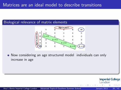
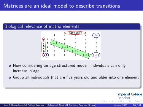
Now considering an age structured model individuals can onlyincrease in age
Group all individuals that are five years old and older into one element
Individuals ageing by one year (diagonal)
Ana I. Bento Imperial College London Advanced Topics-II Southern Summer School January 2013 28 / 41
Matrices are an ideal model to describe transitions
Biological relevance of matrix elements
Now considering an age structured model individuals can onlyincrease in age
Group all individuals that are five years old and older into one element
Individuals ageing by one year (diagonal)
Ana I. Bento Imperial College London Advanced Topics-II Southern Summer School January 2013 28 / 41

Matrices are an ideal model to describe transitions
Using the fundamental equation for each class
Nt+1 = Nt,axSa + Nt,ixRixSi
Where:
Nt,a = number of adult females at time t
Nt,i = number of immature females at time t
Sa = annual survival of adult females from time t to time t+1
Si = annual survival of immature females from time t to time t+1
Ri = ratio of surviving young females at the end of the breedingseason per breeding female
Ana I. Bento Imperial College London Advanced Topics-II Southern Summer School January 2013 29 / 41

Matrices are an ideal model to describe transitions
In a matrix notation
Ana I. Bento Imperial College London Advanced Topics-II Southern Summer School January 2013 30 / 41

Matrices are an ideal model to describe transitions
In a matrix notation
Each row in the first and third matrices corresponds to animals withina given age range (0 to1 years, 1 to 2 years and 2 to 3 years).
The top row of the middle matrix consists of age-specific fertilities:F1, F2 and F3.
These models can give rise to interesting cyclical or seemingly chaoticpatterns in abundance over time when fertility rates are high
The terms Fi and Si can be constants or they can be functions ofenvironment, such as habitat or population size. Randomness canalso be incorporated into the environmental component (as we willsee tomorrow).
Ana I. Bento Imperial College London Advanced Topics-II Southern Summer School January 2013 31 / 41

Matrices are an ideal model to describe this transition
Examples of matrices from biological systems
Blue parts of the matrices represent non-zero elements
Ana I. Bento Imperial College London Advanced Topics-II Southern Summer School January 2013 32 / 41

How do matrices work
How can we analyse matrices
Observed (average per capita) population growth rate
In year t+1 the population is 71.6 % as large as it was in year t. Onaverage one individual in year t is only 0.716 individuals in year t+1(hence the per capita bit)
Ana I. Bento Imperial College London Advanced Topics-II Southern Summer School January 2013 33 / 41
How do matrices work
λ = per capita population growth rate when the population is atequilibrium or long-term population growth rate. This is the dominanteigenvalue of the matrix.
ω= per capita population growth rate given an observed populationvector If a population structure is at equilibrium, then λ = ω
When λ >1 the population is growing, λ <1 the population isdeclining and λ=1 the population is constant
Ana I. Bento Imperial College London Advanced Topics-II Southern Summer School January 2013 34 / 41
Reproductive value
From the matrix model we can find the right (w) and left (v)eigenvectors of the matrix A associated with the dominant eigenvalue
The right eigenvector w is the stable (st)age distribution or the longterm equilibrium states
The left eigenvector (v) is the reproductive value for the populationat equilibrium
Reproductive value (Fisher 1930): “To what extent will persons ofthis age, on the average, contribute to the ancestry of futuregenerations? This question is of some interest, since the direct actionof Natural Selection must be proportional to this contribution”
Ana I. Bento Imperial College London Advanced Topics-II Southern Summer School January 2013 35 / 41

Reproductive value
Function of both recruitment and survival probability. For mostvertebrates reproductive value peaks with young breeding adults
Ana I. Bento Imperial College London Advanced Topics-II Southern Summer School January 2013 36 / 41

Sensitivity
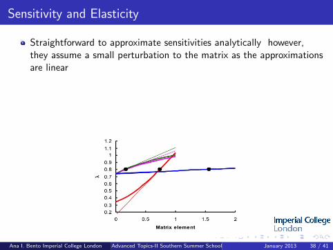
The association between a matrix element and λ. What wouldhappen to λ if a matrix element was perturbed?
Black dots representλ for the unperturbed matrix. Thick lines =actual consequences. Thin lines = linear approximations
Ana I. Bento Imperial College London Advanced Topics-II Southern Summer School January 2013 37 / 41

Sensitivity
The association between a matrix element and λ. What wouldhappen to λ if a matrix element was perturbed?
Black dots representλ for the unperturbed matrix. Thick lines =actual consequences. Thin lines = linear approximations
Ana I. Bento Imperial College London Advanced Topics-II Southern Summer School January 2013 37 / 41
Sensitivity and Elasticity
Straightforward to approximate sensitivities analytically however,they assume a small perturbation to the matrix as the approximationsare linear
Elasticities = proportional sensitivities (i.e. they sum to one)
To identify the key demographic rate associated with λ can targetdemographic rates with high sensitivites / elasticities for conservation/ bio-control
Ana I. Bento Imperial College London Advanced Topics-II Southern Summer School January 2013 38 / 41

Limitations of matrices
Most frequently used analysis assume the population is at equilibriumstructure
No variation is demographic rates
Ways to get around this
Demographic rates varying from year to year incorporatingenvironmental variation (adding stochasticity)
Ana I. Bento Imperial College London Advanced Topics-II Southern Summer School January 2013 39 / 41

Stochastic matrices
What if demographic rates vary with time?
Instead of working with average lambda well want to work with thelong-run stochastic growth rate
Demographic rates varying from year to year incorporatingenvironmental variation
Are methods to calculate the long-run stochastic growth rate fromrandom matrices, as well elasticities and sensitivities
We will see an example tomorrow
Also see papers by Tuljapurkar et al.
Ana I. Bento Imperial College London Advanced Topics-II Southern Summer School January 2013 40 / 41

Summary
Basic concepts of population and demography
Structured populations
Modelling framework for age or stage structured populations
Discrete time models are the most often used - especially matrices
Ana I. Bento Imperial College London Advanced Topics-II Southern Summer School January 2013 41 / 41