“advanced topics in finance and engineering: extreme value theory (evt), risk management, and...

“Advanced Topics in Finance and Engineering: Extreme Value Theory (EVT), Risk Management,

and Applications” Econ. & Mat. Enrique Navarrete

Palisade Risk ConferenceRio de Janeiro 2009

CONFERENCE

Extreme Value Theory

TOPICS:

• Introduction and motivation;• Use of the Gumbel distribution (Extreme Value

Distribution);• Use of the Generalized Extreme Value Distribution (GEV);

– Parameter estimation by Maximum Likelihood (MLE);– Identification of the tail parmeter (Hill’s method);– Estimation of extreme loss percentiles;

Examples

®Scalar Consulting, 2009

INTRODUCTION TO EXTREME VALUE

THEORY (EVT)


Motivation:• Maximum insurance claims (monthly maxima, N = 90

months)


Frauds (x)1 $256.9132 $150.0193 $151.5634 $154.1555 $156.4776 $158.5537 $161.5148 $162.8659 $166.021

10 $169.75311 $170.93012 $173.78613 $176.82814 $178.99315 $182.07316 $184.28817 $186.02418 $187.93719 $192.36920 …

What is the “maximimun” claims level we can expect ?

By simulation methods, could we expect to get a number larger than

the historical maximum?

70 …71 $407.37172 $419.05373 $421.36874 $430.99475 $444.76476 $446.24077 $455.95378 $463.73079 $474.91580 $487.68781 $494.44782 $507.04083 $518.97384 $533.72385 $550.38486 $557.65087 $577.51288 $585.97489 $606.91590 $633.334

Fraudes sobre $ 150,000

$0

$50.000

$100.000

$150.000

$200.000

$250.000

$300.000

$350.000

$400.000

$450.000

$500.000

1 8 15 22 29 36 43 50 57 64 71

Pérdidas

Val

or

de

la P

érd

ida


Motivation:• = RiskWeibull(1,2171;172469;RiskShift(144825))


99,0% 1,0%

−∞ 0,749

0,0

0,2

0,4

0,6

0,8

1,0

1,2

1,4

Values in Millions ($)

0,0

0,5

1,0

1,5

2,0

2,5

3,0

3,5

4,0

4,5

Val

ue

s x

10

^-6

Weibull

Weibull

Minimum$144844,0368Maximum$1366916,6887Mean $306486,7506Std Dev $133527,4049Values 10000

Weibull

p x0,99 749.000

0,995 823.0000,999 987.000


Motivation:• = RiskWeibull(1,2171;172469;RiskShift(144825))


Weibull

p x0,99 749.000

0,995 823.0000,999 987.000

For monthly data, how often should we expect to see the values at the 99,5 % and 99,9 % levels ?


Related Question:

• If the chance of volcanic eruption today is 0,006 %, how do we interpret this small probability ?



Related Question:

• If

* N

then:

N = 1/ (0,006 %) = 16,666 days

= 45,6 years®Scalar Consulting, 2009

N (time window to see an event) = 1 / Probability

N (number of days) * Daily probability = 1 event


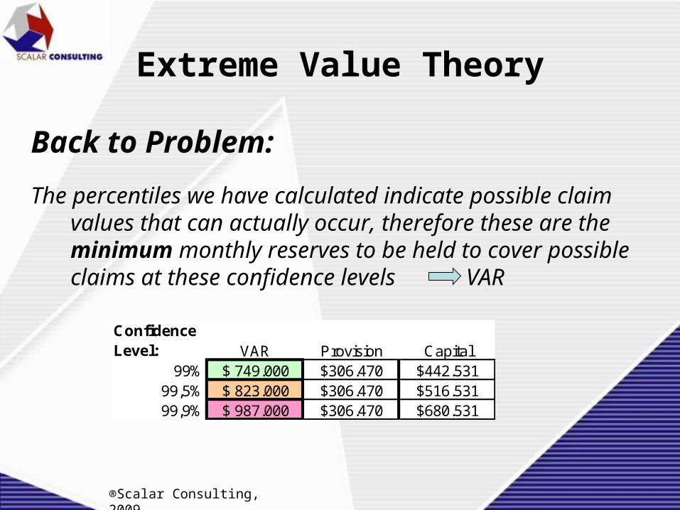
Back to Problem:

The percentiles we have calculated indicate possible claim values that can actually occur, therefore these are the minimum monthly reserves to be held to cover possible claims at these confidence levels VAR


ConfidenceLevel: VAR Provision Capital

99% $ 749.000 $306.470 $442.53199,5% $ 823.000 $306.470 $516.53199,9% $ 987.000 $306.470 $680.531


Back to Problem:

Now these confidence levels have failure rates:

Example: By setting up a monthly reserve of $ 823,000 (VAR 99,5 %), we would expect to cover all claims approximately 199/200 months (= 99,5 %) and will not be able to cover claims approx. 1 every 200 months


How many How manyCovers Fails months years

VAR 99 % 99% 1% 100 8,3VAR 99,5 % 99,5% 0,5% 200 16,7VAR 99,9 % 99,9% 0,1% 1000 83,3


Application:

How do we set an appropriate level of monthly reserves that fails (falls short of claims) approximately once every 2 years ?



Application:

How do we set a appropriate level of monthly reserves that fail (fall short of claims) approximately once every 2 years ?

Failure rate = (1/24 ) months = 4,2 %

Confidence level = (1 - 1/24) = 95,8%

VAR 95,8% = $ 590,000.



More Applications:

• How high should we build a dam that fails (allows flooding) once every 40 years ?

• How strong to build homes to support hurricanes and collapse every 80 years ?

• How resistant to build antennae in presence of very strong winds ?

• How strong to build materials in general?


EXTREME VALUE THEORY AND APPLICATIONS


Generalized Extreme Value Distribution (GEV):

• Under certain conditions, the GEV distribution is the limit distribution of sequences of independent and identically distributed random variables.

= location parameter; = scale parameter = shape (tail) parameter



Fisher-Tippett-Gnedenko Theorem:


Loss Distribution

Pro

bab

ilit

y

$

Only 3 possible families of distributions for the maximumm depending on the parameter !

> 0 (Fréchet)

= 0 (Gumbel)

< 0 (Reversed Weibull)



• For modeling maxima, the case < 0 is not interesting (“thin tails”);

• For the case (Gumbel), we can take shortcuts and avoid estimating the tail parameter;

use Gumbel (Extreme Value Distribution);

• For the case > 0 (“fat tails”), we have to use the GEV Distribution and estimate the tail parameter (Hill’s Plot).


Gumbel Distribution(Extreme Value Distribution)

= 0


Location and Scale parameters (MOM):

1) Obtain sample mean ( ) and sample standard deviation (s) from the series of maxima;

2) We are assuming initially that the distribution is Gumbel ( = 0);

3) Estimate location ( ) and scale parameters ( ) using formulas from Method of Moments (MOM);


x

x

s 6

Formulas apply to Gumbel distribution


Location and Scale parameters (MOM):

where = Euler´s Constant :

.


577216,0

Limiting difference between the harmonic series and the natural

logarithm


Example 1: (MOM)• Maximum losses (monthly, N = 60)


Sample

sample mean 69.117sample std dev 51.935

Gumbel MOM Percentiles:p x

0,99 232.0200,9917 239.6000,995 260.1900,999 325.444

Loss Plot Position 11 225.500 99,17%2 200.000 97,50%3 190.000 95,83%4 185.000 94,17%5 150.000 92,50%6 140.000 90,83%7 135.000 89,17%8 130.000 87,50%9 120.000 85,83%

10 118.000 84,17%11 113.000 82,50%12 110.000 80,83%13 … 79,17%

MOM (Gumbel)

location 45.743scale 40.494


Location and Scale parameters (MLE):

• As an alternative to MOM, we can calculate the location

and scale parameters by Maximum Likelihod Estimation

ie. and that maximize the function:

N

i

iN

i

i xxN

11

expln



Example 1: (MLE)• Maximum losses (monthly, N = 60)



10 118.000 84,17%11 113.000 82,50%12 110.000 80,83%13 … 79,17%

MLE MOM (Gumbel) 46.170 location 45.743 37.286 scale 40.494

Gumbel MLE Percentiles: Gumbel MOM Percentiles:p x p x0,99 217.690 0,99 232.020

0,9917 224.669 0,9917 239.6000,995 243.628 0,995 260.1900,999 303.712 0,999 325.444


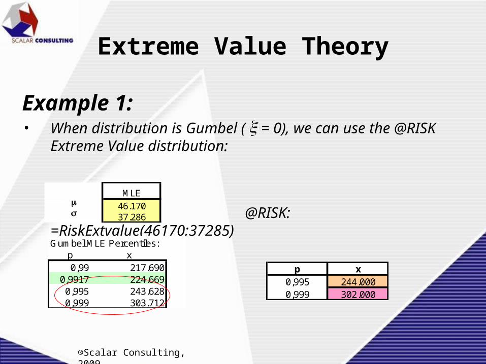
Example 1:• @RISK: =RiskExtvalue(46170;37285)

p x0,995 244.0000,999 302.000



Example 1:• When distribution is Gumbel ( = 0), we can use the @RISK

Extreme Value distribution:

@RISK: =RiskExtvalue(46170;37285)

p x0,995 244.0000,999 302.000


Gumbel MLE Percentiles: Gumbel MOM Percentiles:p x p x0,99 217.690 0,99 232.020

0,9917 224.669 0,9917 239.6000,995 243.628 0,995 260.1900,999 303.712 0,999 325.444


Generalized Extreme Value Distribution (GEV)

> 0



• Since in general , we need to estimate this parameter by Hill’s Method.

• Graph of:

0






To get the loss percentiles we need to estimate the shape parameter


10 118.000 84,17%11 113.000 82,50%12 110.000 80,83%13 … 79,17%

Location and scale parameters are very different, suggesting distribution

is not Gumbel


Example 2:• Hill’s Diagram


Hill Plots

0,000

0,500

1,000

1,500

2,000

2,500

1 5 9 13 17 21 25 29 33 37 41 45 49 53 57

Hill Plot 1

Hill Plot 2

= 0,4





10 118.000 84,17%11 113.000 82,50%12 110.000 80,83%13 … 79,17%

p x p x0,99 262.692 0,99 732.769

0,9917 271.377 0,9917 799.8840,995 294.968 0,995 840.5930,999 369.732 0,999 1.612.214

MLEGumbel EV Percentiles: GEV Percentiles:

MLE

We obtain very different GEV percentiles since the distribution is

not Gumbel ( ).0


Example 2:

• Since , we cannot use the Gumbel distribution; either estimate and use EVT or use a @RISK distribution, (not the Extreme value Distribution ie.Gumbel) since it will stay short.

0



Example 2:• @RISK: =RiskPearson5(2,2926;124899;RiskShift(-12413))

p x0,995 767.0000,999 1.593.000



Example 1 (Gumbel):• Hill’s Plot


= 0.06 (ie. for all practical purposes the

distribution is Gumbel)

Hill Plots

0,000

0,500

1,000

1,500

2,000

1 5 9 13 17 21 25 29 33 37 41 45 49 53 57

Hill Plot 1

Hill Plot 2


Example 3:• Hill’s Plot


Hill Plots

0.000

0.200

0.400

0.600

0.800

1.000

1 3 5 7 9 11 13 15 17 19 21

Hill Plot 1

Hill Plot 2

= 0.01 (Gumbel)


Example 4:• Hill’s Plot


= 0.38 (not Gumbel,

use GEV)

Hill Plots

0,000

0,500

1,000

1,500

2,000

2,500

1 2 3 4 5 6 7 8 9 10 11 12 13

Hill Plot 1

Hill Plot 2

Enrique Navarrete , Scalar Consulting

• www.grupoescalar.com• [email protected] • MSc. University of Chicago• BS. Economics, BS. Mathematics, MIT• Risk Software, Consulting and Auditing• Risk courses offered jointly with Universidad

Iberoamericana, several countries

“advanced topics in finance and engineering: extreme value theory (evt), risk management, and...

Documents