advanced topic 6: exchange rate determination iiihomes.chass.utoronto.ca/~floyd/atexrdt3.pdfadvanced...

Advanced Topic 6:

Exchange Rate Determination III

John E. FloydUniversity of Toronto

July 16, 2013

The analysis below involves an empirical investigation of the role of real shocks indetermining movements in real exchange rates. The task is to try to determinethe extent to which observed real exchange rate changes are a consequence of realshocks to technology and capital accumulation. Given the lack of useful modelsof technological change, we can only attempt to discern whether observed realexchange rate movements can be statistically explained by factors such as incomegrowth, terms of trade changes, world oil and commodity price changes, shiftsin world investment, and differential changes in government activity, that wouldobviously be expected to influence countries’ real exchange rates. To investigatethe frequent claim that an increase in domestic/foreign interest differentials arisingfrom monetary policy will cause capital inflows and real exchange rate appreciation,we must create additional regressions that are augmented by adding the interestrate differential to the variables that were otherwise statistically significant.

On the basis of earlier theoretical analysis, we have to conclude that the ar-gument that monetary policy affects exchange rates through its effects on interestrate differentials makes no economic sense for two reasons. First, central banks willnot be able to affect overall domestic/foreign real interest rate differentials by mon-etary expansion because those differentials are determined in world asset markets,although the monetary authories in big countries will be able to affect the overalllevel of world interest rates. And second, the view that international capital flowsrespond to interest rate differentials involves a fallacy of composition. While anyone individual might well shift her portfolio in towards securities whose interestrates have risen, when everyone tries to do this they reduce the demand for thelower-interest-rate securities and increase the demand for the higher-interest-ratesecurities, causing the higher interest rates to fall and/or the lower interest ratesto rise until there is no gain from shifting portfolios. Interest rate differentials aredetermined by the willingness of world asset holders to hold the existing stocks ofthe various securities—actual aggregate asset flows are not required.

To the extent that interest rate differentials and real exchange rates are re-lated, the relation must be in the reverse direction to that postulated above—domestic/foreign interest rate differentials clearly could change as a consequenceof the behaviour of real forces that lead to real exchange rate changes, or perhapsin response to movements of real exchange rates. For that reason, we also run OLSregressions of the interest rate differentials on the same factors that have been shown to causemovements in a country’s real exchange rate with respect to the U.S., including among theindependent variables the real exchange rate itself.

We start withCanada vs. the United States. Below are three Tables of regression resultsinterspersed with plots showing the response of the real exchange rate to various statisticallysignificant real forces. The real exchange rate is defined using, alternatively, the im-plicit GDP deflators and the consumer price indexes as measures of the price levels.The real commodity price variable is an index of world prices of commodities ex-cluding energy in U.S. dollars divided by an equal weighted index of U.S. exportand import prices. The energy price variable is an index of world energy prices inU.S. dollars divided by the equal weighted index of U.S. export and import prices.The real net capital inflow variable is the excess of Canadian imports of goodsand services over exports of goods and services as a percentage of Canadian GDPminus the excess of U.S. imports of goods and services over U.S. exports of goodsand services as a percentage of U.S. GDP. The government consumption expendi-ture variable is Canadian government consumption expenditure as a percentage ofGDP minus U.S. government consumption expenditure as a percentage of GDP.The Canadian and U.S. terms of trade are the countries’ export prices dividedby their import prices. The real GDP variables are constructed by dividing GDPby the implicit GDP deflator. The employment rate variables, which were onlyavailable from 1976Q1, are constructed by subtracting the country’s percentageof labour force unemployed from 100. And the interest rate differentials are ob-tained by subtracting the relevant U.S. interest rate from the Canadian one. In thethree left-most regressions in Table 1, the real exchange rate is constructed using the countries’consumer price indexes while in the three right-most regressions it is constructed using thecountries’ implicit GDP deflators. The three regressions on the left are ones used in InterestRates, Exchange Rates and World Monetary Policy while the three on the right take advantageof additional data available since the book was published and also include the Canadian andU.S. employment rates as independent variables. The addition of these employment ratesresulted in the real GDP variables becoming statistically significant. While theratio of the Canadian to the United States terms of trade was statistically insignif-icant, a significant coefficient with the expected positive sign was obtained whenthe Canadian terms of trade alone was used. Basing the real exchange rate on theimplicit GDP deflators rather than the consumer price indexes resulted in a statis-tically significant coefficient for the government expenditure variable. Logarithmsof all variables other than those representing differences in percentages were used.

2

Table 1: OLS regression analysis of real factors affecting the real exchange rate: Canada vs.United States, 1974:Q1 to 2010:Q4

Independent Dependent VariableVariables Logarithm of Real Exchange Rate

1974Q1 — 2007Q4 1976Q1 — 2010Q4

2.612 2.369 2.292 2.206 1.205 0.620Constant (0.187)∗∗∗ (0.185)∗∗∗ (0.186)∗∗∗ (1.102)∗∗ (0.894) (0.872)

Log of Com- 0.310 0.372 0.388 0.441 0.529 0.529modity Prices (0.065)∗∗∗ (0.068)∗∗∗ (0.071)∗∗∗ (0.118)∗∗∗ (0.104)∗∗∗ (0.106)∗∗∗

Log of 0.154 0.134 0.132 0.140 0.156 0.158Energy Prices (0.034)∗∗∗ (0.034)∗∗∗ (0.034)∗∗∗ (0.034)∗∗∗ (0.030)∗∗∗ (0.030)∗∗∗

Real Net 0.028 0.022 0.021 0.026 0.025 0.024Capital Inflow (0.004)∗∗∗ (0.004)∗∗∗ (0.005)∗∗∗ (0.004)∗∗∗ (0.003)∗∗∗ (0.003)∗∗∗

Gov’t Consumption 0.023 0.008 0.004Expenditure (0.014)∗∗ (0.011) (0.011)

Log of Canadian 0.738 0.639 0.666Terms of Trade (0.285)∗∗∗ (0.245)∗∗∗ (0.247)∗∗∗

Log Canadian 2.593 1.733 1.279Real GDP (0.520)∗∗∗ (0.408)∗∗∗ (0.414)∗∗∗

Log U.S. -2.288 -1.479 -1.050Real GDP (0.459)∗∗∗ (0.361)∗∗∗ (0.369)∗∗∗

Canadian -0.040 -0.045 -0.040Employment Rate (0.009)∗∗∗ (0.008)∗∗∗ (0.008)∗∗∗

U.S. 0.032 0.032 0.027Employment Rate (0.009)∗∗∗ (0.007)∗∗∗ (0.007)∗∗∗

1-Month 3-Month 1-Month 3-MonthCorporate Tresury Corporate TreasuryPaper Bills Paper Bills

Interest Rate 0.015 0.017 0.017 0.022Differential (0.004)∗∗∗ (0.004)∗∗∗ (0.003)∗∗∗ (0.004)∗∗∗

Num. Obs. 136 136 136 140 140 140R-Squared .775 .802 .808 .835 .865 .870

Note: The variables are defined in the main text. The figures in brackets are the heteroskedasticity andautocorrelation adjusted coefficient standard errors calculated in the Gretl statistical program, which chosea band width of 3 and a bartlett kernel. Significant serial correlation was present in the residuals of allregressions. The superscripts ∗∗∗ indicate significance at the 1% levels according to a standard t-test.

3

The real exchange rate is positively related, as our theory suggests, to commod-ity prices, energy prices, the excess of Canadian over U.S. net capital inflows aspercentages of their GDPs, the excess of Canadian over U.S. government consump-tion expenditures as percentages of their GDPs, and the Canadian terms of tradewith respect to the rest of the world. And the two interest rate differential variables thatwere added in turn were all significantly positively related to the relevant real exchange rates.The sign of the Canadian real GDP variable is positive and the sign of the U.S. realGDP variable is negative as consistent with the Balassa-Samuelson hypothesis andthe employment rate variables have opposite signs to the real GDP variables as isconsistent with our expectation that a temporary increase in a country’s outputshould reduce its value in world markets. The R-square in the 1976Q1 through 2010Q4regression was .835. The plots in Figure 1 below indicate that the major movementsprior to year 2000 are quite well explained by the real net capital inflow variableand after 2000 by commodity and energy prices. The other statistically significantvariables did not have effects on the real exchange rate that were visible to thenaked eye.1

Someone might try to argue that the regression results in Table 1 above could be spurious.When a unit-root variable is regressed on other unit-root variables, statistically significant coef-ficients will often arise even though the unit-root variables involved may be totally independentof each other. There are three reasons why the above regression results could notbe spurious. First, there are stationary independent variables in each regression—in particular the commodity price variable and the interest rate differentials. Forthese stationary variables to be statistically significant they must be correlated with the resid-uals of a regression that includes only the non-stationary variables, which can only happenif those residuals are stationary—for that regression to be spurious, its residuals would haveto be non-stationary. Second, while it is possible for a regression involving two orthree totally independent non-stationary variables to yield statistically significantresults, the chances of a regression of one non-stationary variable on nine othernon-related variables producing nine statistically significant coefficients with theexpected signs is virtually zero. Third, for the sake of argument a Johansen cointe-gration test was conducted in Gretl on the three non-stationary variables consistingof the logarithm of the real exchange rate, the net capital inflow difference and thelogarithm of energy prices for the period 1974Q1 through 2007Q4.2 The hypothesisof no-cointegration—that is, that the relationship between them is spurious—couldbe rejected at the 1% level.3 Since these variables are cointegrated, all the regressions inthe Table must be non-spurious since all the coefficients are statistically significant.

1This econometric work for the 1974Q1–2007Q4 period was performed alternatively in Gretl, and XLispStat

using the respective input files rexcaus.inp and rexcaus.lsp which, using the respective data files jfdataqt.gdtand jfdataqt.lsp, produced the output files rexcaus.got, rexcaus.lou. The data are also in the Excel spread-sheet file jfdataqt.xls. The sources are explained in the Gretl data file jfdataqt.gdt and in the text filejfdataqt.cat. The calculations for the period 1976Q1–2010Q4 were performed in a Gretl session for which thesession file is causrex.gretl, which contains and properly describes all the data used and the output produced.

2For a discussion of the nature of this test, see pages 385-400 of the Enders book cited in the course outline.It is also discussed more briefly on page 166 of Interest Rates, Exchange Rates and World Monetary Policy.

3The variables were first tested for stationarity in Gretl using augmented Dickey-Fuller tests and the null-hypothesis of stationarity could easily be rejected in all three cases.

4

Quarterly

Loga

rithm

s of

Mea

n E

quiv

alen

t Lev

els

1975 1980 1985 1990 1995 2000 2005 2010

4.5

4.6

4.7

4.8

4.9

Real Exchange RateEffect of Net Capital Inflows

Quarterly

Loga

rithm

s of

Mea

n E

quiv

alen

t Lev

els

1975 1980 1985 1990 1995 2000 2005 2010

4.5

4.6

4.7

4.8

4.9

Real Exchange RateEffect of Energy Prices

Figure 1: The effects of real net capital inflows energy prices and the prices of commoditiesexclusive of energy on the Canadian real exchange rate with respect to the United States.

5

The fact that the interest rate variables were positively signed and statistically significantin the regressions in Table 1 might be taken as support for the view that capital flows area function of interest rate differentials which are determined by the monetary authorities ofthe respective countries. The fact that there is no theoretical basis for this view requires analternative explanation of what is observed. Indeed, it is quite reasonable to argue thatthe observed interest rate differentials might be explained by the same variablesthat determine real exchange rates as well as by the real exchange rate itself. Thatis, the causality of the observed relationship between the real exchange rate andinterest rate differentials may be the direct opposite of that implied by the realexchange rate regressions in the table above. To check this out we run regressions of theinterest rate differentials on the real exchange rate and the variables found to explain it. Theseinterest rate differential regressions presented in Table 2 below for the period 1976Q1 through2010Q4. The U.S. employment rate and net capital inflow variables were insignificant in theT-Bill rate regression and were therefore dropped.4

A potential interpretation of these results is that increases in the real exchange rate andCanadian relative to U.S. real income and employment increase the risk of holding Canadian ascompared to U.S. assets while increases in commodity and energy prices, net capital inflows andgovernment consumption expenditure reduce that relative risk. Given that the real exchangerate and the differences in income and employment have no trend, high levels of these variablesincrease the probability of future declines and low levels increase the probability of futureincreases. Increased Canadian relative to U.S. government consumption expenditure wouldreduce the risk by making future increases in income more likely. And increased capital inflows,higher prices of commodities and energy and an improvement in the terms of trade, at givenlevels of income and employment and the real exchange rate, reduce the risk because theysignify that Canada is better off. The problem with this interpretation is that it is difficultto imagine that the default risk on treasury bills and would change as a result ofthe magnitudes of changes in real exchange rates and commodity prices that havebeen observed.

An alternative approach would explain the coefficients of the variables as reflect-ing the correlation of changes in those variables with expected future Canadianinflation relative to that in the United States. Expansion of income and employ-ment in a country might tend to increase the prospect of domestic inflation, Andincreases in commodity and energy prices, net capital inflows and the terms oftrade, holding real incomes and the price of domestic output in terms of foreignoutput constant, would tend to increase the supply of domestic output with theresult that the upward pressure on domestic nominal prices will be smaller. And,holding other things constant, an increase in the real exchange rate—that is, theprice of domestic in terms of foreign output—might be expected to exert upwardpressure on domestic nominal prices.

4The analysis here is performed entirely in the Gretl session causrex.gretl.

6

Table 2: OLS Regression analysis of real Factors affecting interest rate differentials: Canadavs. United States, 1976:Q1 to 2010:Q4

Dependent Variables: Interest Rate DifferentialsIndependentVariables 1-Month 3-Month

Corporate TreasuryPaper Bills

Constant 40.092 57.837(16.349)∗∗∗ (14.294)∗∗∗

Log of Energy Prices -1.452 -0.837(0.610)∗∗∗ (0.478)∗∗

Log of Commodity Prices -9.213 -7.626(1.932)∗∗∗ (1.766)∗∗∗

Net Capital Inflow -0.180(0.090)∗∗

Government Consumption -0.668 -0.551(0.274)∗∗∗ (0.227)∗∗∗

Log of Canadian Terms of Trade -6.419 -6.297(2.706)∗∗∗ (2.428)∗∗∗

Log of Canadian Real GDP 24.163 37.242(12.304)∗∗ (9.558)∗∗∗

Log of U.S. Real GDP -23.915 -35.882(10.995)∗∗ (8.480)∗∗∗

Canadian Employment Rate 0.718 0.459(0.200)∗∗∗ (0.127)∗∗∗

U.S. Employment Rate -0.316(0.177)∗∗

Log of Real Exchange Rate 10.793 7.788(2.127)∗∗∗ (1.578)∗∗∗

Num. Obs. 140 140R-Squared .605 .708Adjusted R-Squared .575 .690

Note: The figures in the brackets ( ) are the heteroskedastic and autocorrelation adjustedstandard errors calculated in the Gretl statistical program, which chose a band width of 3 anda bartlett kernel. The superscripts ∗∗∗ indicate significance at the 1% levels according to astandard t-test. The adjusted R-Squared is adjusted for degrees of freedom.

7

Table 3: OLS Regression analysis of relationship between interest rate and inflation rate differ-entials: Canada vs. United States, 1975:Q1 to 2010:Q4

Dependent Variables: Interest Rate DifferentialsIndependentVariables 1-Month 3-Month

Corporate TreasuryPaper Bills

Constant 1.096 1.429(0.225)∗∗∗ (0.237)∗∗∗

Inflation Rate Differential 0.336 0.314(0.097)∗∗∗ (0.097)∗∗∗

Num. Obs. 140 140R-Squared .120 .107Adjusted R-Squared .113 .101

Note: The interest rate differentials are those in Table 1 and the inflation differential is theexcess of the Canadian over U.S. year-over-year CPI inflation rate. The figures in bracketsare the heteroskedastic and autocorrelation adjusted standard errors calculated in the Gretlstatistical program, which chose a band width of 3 and a bartlett kernel. The superscripts ∗∗∗

indicate significance at the 1% levels according to a standard t-test. The adjusted R-squaredis adjusted for degrees of freedom.

8

In this respect, it is interesting that the excess of the Canadian over theU.S. year-over-year inflation rate was insignificant when added to the regressions inTable 2. Yet this variable is always significant with the expected positive sign whenit is the only explanatory variable, as shown in Table 3 above, but the R-squares,both unadjusted and adjusted for degrees of freedom, are very low compared tothose in the Table 2 regressions. This is consistent with the interpretation thatthe variables in the latter regressions are indeed capturing changes in the expectedfuture inflation differential—they encompass all explanatory power contained inthe inflation differential over the previous year, suggesting that the real variablesindirectly reflect both the actual and expected differences in Canadian relative toU.S. inflation. Final conclusions regarding the determination of the Canada/U.S. interestrate differential must nevertheless wait until monetary shocks are introduced into the analysis.

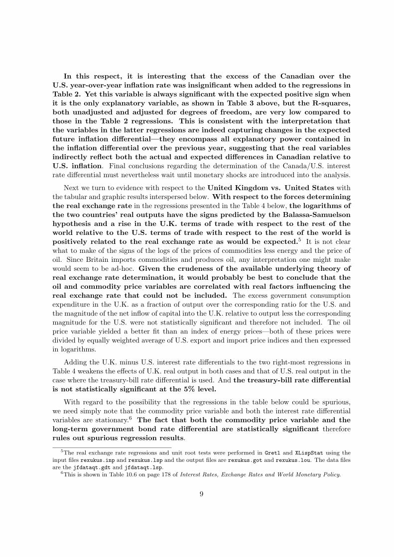
Next we turn to evidence with respect to the United Kingdom vs. United States withthe tabular and graphic results interspersed below. With respect to the forces determiningthe real exchange rate in the regressions presented in the Table 4 below, the logarithms ofthe two countries’ real outputs have the signs predicted by the Balassa-Samuelsonhypothesis and a rise in the U.K. terms of trade with respect to the rest of theworld relative to the U.S. terms of trade with respect to the rest of the world ispositively related to the real exchange rate as would be expected.5 It is not clearwhat to make of the signs of the logs of the prices of commodities less energy and the price ofoil. Since Britain imports commodities and produces oil, any interpretation one might makewould seem to be ad-hoc. Given the crudeness of the available underlying theory ofreal exchange rate determination, it would probably be best to conclude that theoil and commodity price variables are correlated with real factors influencing thereal exchange rate that could not be included. The excess government consumptionexpenditure in the U.K. as a fraction of output over the corresponding ratio for the U.S. andthe magnitude of the net inflow of capital into the U.K. relative to output less the correspondingmagnitude for the U.S. were not statistically significant and therefore not included. The oilprice variable yielded a better fit than an index of energy prices—both of these prices weredivided by equally weighted average of U.S. export and import price indices and then expressedin logarithms.

Adding the U.K. minus U.S. interest rate differentials to the two right-most regressions inTable 4 weakens the effects of U.K. real output in both cases and that of U.S. real output in thecase where the treasury-bill rate differential is used. And the treasury-bill rate differentialis not statistically significant at the 5% level.

With regard to the possibility that the regressions in the table below could be spurious,we need simply note that the commodity price variable and both the interest rate differentialvariables are stationary.6 The fact that both the commodity price variable and thelong-term government bond rate differential are statistically significant thereforerules out spurious regression results.

5The real exchange rate regressions and unit root tests were performed in Gretl and XLispStat using theinput files rexukus.inp and rexukus.lsp and the output files are rexukus.got and rexukus.lou. The data filesare the jfdataqt.gdt and jfdataqt.lsp.

6This is shown in Table 10.6 on page 178 of Interest Rates, Exchange Rates and World Monetary Policy.

9

Table 4: OLS Regression analysis of real factors affecting the real exchange rate: United King-dom vs. United States, 1974:Q1 to 2007:Q4


Constant -2.043 -3.609 -4.391(1.282) (1.309)∗∗∗ (1.356)∗∗∗

Log of Com- 0.466 0.513 0.359modity Prices (0.085)∗∗∗ (0.072)∗∗∗ (0.081)∗∗∗

Log of -0.206 -0.184 -0.174Oil Prices (0.051)∗∗∗ (0.053)∗∗∗ (0.038)∗∗∗

Log of Terms 1.835 1.846 1.932of Trade Ratio (0.213)∗∗∗ (0.225)∗∗∗ (0.200)∗∗∗

Log of U.K. 2.216 1.714 1.432Real GDP (0.731)∗∗∗ (0.786)∗∗ (0.556)∗∗

Log of U.S. -1.619 -1.191 -0.905Real GDP (0.586)∗∗∗ (0.632)∗ (0.451)∗∗

Treasury Long-TermBills Gov’t Bonds

Interest Rate 0.012 0.027Differential (0.006)∗ (0.008)∗∗∗

Num. Obs. 136 136 136R-Square .720 .748 .770

Note: The real exchange rate is CPI based and the commodity price and energy price variables are the

same as those used in the Canadian case. The interest rate differentials are U.K. minus U.S. The figures

in brackets are the heteroskedasticity and autocorrelation adjusted coefficient standard errors calculated

in the Gretl statistical program, which chose a band width of 3 and a bartlett kernel. Significant

serial correlation was present in the residuals of all regressions. The superscripts ∗∗∗, ∗∗ and ∗ indicate

significance at the 1%, 5% and 10% levels respectively.

10

40

60

80

100

120

140

160

1975 1980 1985 1990 1995 2000 2005

1975 = 100

Real Exchange RateNominal Exchange Rate

Price Level Ratio

Figure 2: Real and nominal exchange rates of the United Kingdom with respect to the UnitedStates and the ratio of the United Kingdom over United States price level, 1975 = 100.

4.4

4.5

4.6

4.7

4.8

4.9

5

5.1

5.2

1975 1980 1985 1990 1995 2000 2005

U.K. / U.S. REAL EXCHANGE RATE: ACTUAL AND FITTED BASED ON REAL FACTORS

Logarithm of ActualLogarithm of Fitted

Figure 3: The real exchange rate of the United Kingdom with respect to the United States:Actual and fitted levels in logarithms.

The real and nominal exchange rates of the United Kingdom with respect to the UnitedStates and the ratio of the U.K. over the U.S. price levels are plotted in Figure 2 above. Theactual and fitted values in the regression that excludes interest rate differentials are plotted inFigure 3 and contributions of important variables to explaining the real exchange rate move-ments are plotted in Figure 4. The terms of trade ratio provides some explanationof the real exchange rate movements prior to 1985 as well as the increase thatoccurred after 2000. The commodity price variable also seems to explain the risein the real exchange rate after 2000 with the real oil price variable having the op-posite effect, although it is unclear what forces these variables are capturing. Theincome variables simply help explain the trend.

11

4.4

4.5

4.6

4.7

4.8

4.9

5

5.1

5.2

5.3

1975 1980 1985 1990 1995 2000 2005

U.K. / U.S. REAL EXCHANGE RATE: EFFECTS OF PRICES OF COMMODITIES LESS ENERGY

Actual Real Exchange RateDue to Real Commodity Prices

4.4

4.5

4.6

4.7

4.8

4.9

5

5.1

5.2

5.3

1975 1980 1985 1990 1995 2000 2005

U.K. / U.S. REAL EXCHANGE RATE: EFFECTS OF OIL PRICES

Actual Real Exchange RateDue to Oil Prices

4.4

4.5

4.6

4.7

4.8

4.9

5

5.1

5.2

5.3

1975 1980 1985 1990 1995 2000 2005

U.K. / U.S. REAL EXCHANGE RATE: EFFECTS OF RATIO OF U.K. OVER U.S. TERMS OF TRADE

Actual Real Exchange RateDue to Relative Terms of Trade

4.4

4.5

4.6

4.7

4.8

4.9

5

5.1

5.2

5.3

1975 1980 1985 1990 1995 2000 2005

U.K. / U.S. REAL EXCHANGE RATE: COMBINED EFFECT OF U.K. AND U.S. OUTPUTS

Actual Real Exchange RateDue to Combined Real GDPs

Figure 4: The effects of oil prices, the prices of commodities exclusive of energy, the ratio of theU.K. to U.S. terms of trade and the combined effect of U.K. and U.S. outputs on the U.K. realexchange rate with respect to U.S.

12

Table 5: OLS Regression analysis of real factors affecting interest rate differentials: UnitedKingdom vs. United States, 1974:Q1 to 2007:Q4

Dependent Variables: Interest Rate DifferentialsIndependentVariables Treasury Bill Long-Term Gov’t

Interest Rate Bond RateDifferential Differential

Constant 26.858 59.373 119.095(8.825)∗∗∗ (22.511)∗∗∗ (11.000)∗∗∗

Log of Com- -5.766 -4.553modity Prices (1.976)∗∗∗ (1.915)∗∗

Log of Energy 1.534Prices (0.712)∗∗

Difference -0.929 0.441Gov’t Cons. (0.370)∗∗ (0.223)∗∗

Difference 0.593Cap. Inflow (0.169)∗∗∗

Terms of -13.452 -18.875Trade Ratio (4.916)∗∗∗ (3.041)∗∗∗

Log of U.K. 15.302Real GDP (6.416)∗∗

Log of U.S. -16.978Real GDP (5.263)∗∗∗

Log of Real 5.249 7.643Exchange Rate (2.532)∗∗ (1.255)∗∗∗

Inflation Rate 0.244 0.255Difference (0.070)∗∗∗ (0.089)∗∗∗

Num. Obs. 136 136 136Adj. R-Square .426 .297 .782

Note: The variables are defined in the text and in the notes to Table 4. The R-Square statisticsare adjusted for degrees of freedom. The figures in brackets are the heteroskedasticity andautocorrelation adjusted standard errors calculated in the Gretl statistical program, and thesignificance levels shown, in the same way as in Table 4.

13

Table 6: OLS Regression analysis of relationship between interest rate and inflation rate differ-entials: United Kingdom vs. United States, 1974:Q1 to 2007:Q4

Independent Dependent Variables: Interest Rate DifferentialsVariables Treasury Bills Short-Term Gov’t Bonds

Constant 1.889 2.352(0.302)∗∗∗ (0.273)∗∗∗

Inflation Rate 0.257 0.264Differential (0.067)∗∗∗ (0.053)∗∗∗

Num. Obs. 136 136Adj. R-Square .179 .262

Note: The interest rate differentials are defined in Table 4 and the inflation differential is theexcess of the U.K. over U.S. year-over-year CPI inflation rate. The figures in brackets are theheteroskedastic and autocorrelation adjusted standard errors calculated in the Gretl statisticalprogram, which chose a band width of 3 and a bartlett kernel. The superscripts ∗∗∗ indicatesignificance at the 1% levels according to a standard t-test.

With reference to the interest rate differential regressions in Table 5 above it is important tokeep in mind that the risk premiums on government debt will represent the probability of defaultplus the probability of unexpected inflation.7 And the interest rate differentials themselves willdirectly reflect the excess of expected inflation in the U.K. over that in the U.S. It is thereforenot surprising that the inflation rate difference is statistically significant with apositive sign in the treasury bill rate differential regression—greater past inflationtends to generate the expectation of greater future inflation in the short-run. Inthe case of the long-term government bond rate differential, the long-run expectedinflation differential must have been captured by the time patterns of the realvariables rather than by the past inflation rate.

Any interpretation of the coefficients of the real variables in Table 5, however, will involvelittle more than an ad-hoc exercise of theoretical imagination. If one believes that theprobabilities of default are very small and more or less constant, all that can besaid is that a collection of real factors that would be expected to determine thereal exchange rate are also correlated with the U.K. minus U.S. expected inflationrate differential.

7The respective Gretl and XLispStat input files are idfukus.inp and idfukus.lsp and the output files areidfukus.got and idfukus.lou. The data files are the same as referred to in Footnote 5 above.

14

In contrast to the Canada vs. U.S. case, the actual inflation rate differential, obviouslythrough its effect on expectations, is a major independent factor affecting theU.K. minus U.S. interest rate differentials. This can be seen from the fact that the R-Square statistics, adjusted for degrees of freedom, in the regressions in Table 6 using the inflationrate difference as the only independent variable are one-third to one-half the magnitudes of thedegrees-of-freedom-adjusted R-Squares in Table 5.

We turn now to the case of Japan with respect to the United States in the collection oftables and figures that follow. Figure 5 plots the real and nominal exchange rates of Japan withrespect to the United States, along with the ratio of Japanese over the U.S. price level. TheJapanese real exchange rate increased about 100 percent between 1974 and 1995and then has declined by somewhat less than that amount by 2007. The Japaneseprice level fell rather steadily relative to the U.S. price level by about 50 percentfrom the late 1970s to 2007.

0

50

100

150

200

250

300

350

400

1975 1980 1985 1990 1995 2000 2005

1975 = 100


Price Level Ratio

Figure 5: Real and nominal exchange rates of the Japan with respect to the United States andthe ratio of the Japanese over U.S. price level, 1975 = 100.

15

Table 7: OLS Regression analysis of real factors affecting the real exchange rate: Japanvs. United States, 1974:Q1 to 2007:Q4

Independent Dependent VariableVariables Real Exchange Rate

Constant -9.610 -10.038(1.442)∗∗∗ (1.541)∗∗∗

Log of 0.160 0.123Oil Prices (0.051)∗∗∗ (0.053)∗∗

Log of Terms 1.237 1.188of Trade Ratio (0.188)∗∗∗ (0.166)∗∗∗

Gov’t Consumption 0.033Expenditure (0.010)∗∗∗

Net Capital -0.014Inflow (0.006)∗∗

Log of Japanese 1.224 0.817Real GDP (0.182)∗∗∗ (0.153)∗∗

Log of U.S. -1.868 -0.272Real GDP (0.200)∗∗∗ (0.105)∗∗

Interest Rate -0.028Differential (0.007)∗∗∗

Num. Obs. 136 136R-Square .829 .841

Note: The construction of the variables is explained in the text. The figures in brackets arethe heteroskedasticity and autocorrelation adjusted standard errors calculated in the Gretlstatistical program, which chose a band width of 3 and a Bartlett kernel. Significant serialcorrelation was present in the residuals of all regressions. The superscripts ∗∗∗, ∗∗ and ∗indicatesignificance at the 1%. 5% and 10% levels, respectively.

16

4.5

4.6

4.7

4.8

4.9

5

5.1

5.2

5.3

5.4

5.5

1975 1980 1985 1990 1995 2000 2005

JAPAN / U.S. REAL EXCHANGE RATE: ACTUAL AND FITTED BASED ON REAL FACTORS


Figure 6: Actual and fitted values of the logarithm of the Japanese real exchange rate withrespect to the U.S.

In the OLS regression analysis of real factors affecting the CPI-based Japanesereal exchange rate with respect to the U.S. presented in Table 7 above, the loga-rithm of the ratio of the Japanese terms of trade with respect to the rest of theworld over the U.S. terms of trade with respect to the rest of the world is posi-tively related to the real exchange rate and the logarithm of Japanese real GDPis positively related and that of U.S. real GDP is negatively related as consistentwith the Balassa-Samuelson hypothesis.8 The logarithm of U.S. oil prices relativeto the average of U.S. export and import prices and the excess Japanese gov-ernment consumption expenditure as a percentage of GDP over U.S. governmentconsumption expenditure as a percentage of that country’s GDP are positivelyrelated and the excess of the negative of the Japanese trade balance—that is, realnet capital inflow—as a percentage of GDP over the negative of the U.S. tradebalance as a percentage of real GDP has, surprisingly, a negative sign. There is noobvious reason why the sign of the oil prices variable should be positive for Japan.In this respect it must be kept in mind that the results represent a relationshipbetween the variables that undoubtedly suffers from simultaneity bias and left-outvariables. When the Japanese less U.S. interest rate differential on long-term gov-ernment bonds is added to the equation, it comes in with a negative sign and drivesout the government consumption expenditure and real net capital inflow variables.

Figure 6 above plots the actual and fitted values of the Japanese real exchange rate withrespect to the U.S. and Figures 7 and 8 below plot the measured effects of the various inde-pendent variables in the left-most regression in Table 7 on the real exchange rate. It is clearin second panel from the top in Figure 7 that movements in the relative terms oftrade account for a substantial part of the time pattern of the real exchange ratemovements, and it is clear in the second panel from the to in Figure 8 that Japanese realincome growth has had an important influence. The effects of the other variables, apart fromincome growth in the U.S., are not observable on the graphs.

8The relevant Gretl and XLispStat input and output files here are rexjnus.inp, rexjnus.lsp, rexjnus.gotand rexjnus.lou and the data files are the same as used for the U.K. calculations.

17

4.4

4.6

4.8

5

5.2

5.4

1975 1980 1985 1990 1995 2000 2005

JAPAN / U.S. REAL EXCHANGE RATE: EFFECTS OF OIL PRICES

Actual Real Exchange RateDue to Real Oil Prices

4.4

4.6

4.8

5

5.2

5.4

1975 1980 1985 1990 1995 2000 2005

JAPAN / U.S. REAL EXCHANGE RATE: EFFECTS OF JAPANESE OVER U.S. TERMS OF TRADE

Actual Real Exchange RateDue to Relative Term of Trade

4.4

4.6

4.8

5

5.2

5.4

1975 1980 1985 1990 1995 2000 2005

JAPAN / U.S. REAL EXCHANGE RATE: EFFECTS OF JAPANESE LESS U.S. GOVERNMENT CONSUMPTION

Actual Real Exchange RateDue to Government Consumption

Figure 7: Effects on the logarithm of the Japanese real exchange rate with respect to theU.S. of oil prices, the ratio of the Japanese terms of trade with respect to the rest of theworld over the U.S. terms of trade with respect to the rest of the world, and the excess ofJapanese government consumption as a percentage of GDP over U.S. government consumptionas a percentage of U.S. GDP.

18

4.4

4.6

4.8

5

5.2

5.4

1975 1980 1985 1990 1995 2000 2005

JAPAN / U.S. REAL EXCHANGE RATE: EFFECT JAPANESE LESS U.S. REAL NET CAPITAL INFLOWS

Actual Real Exchange RateDue Excess Real Net Capital Inflow

4.4

4.6

4.8

5

5.2

5.4

1975 1980 1985 1990 1995 2000 2005

JAPAN / U.S. REAL EXCHANGE RATE: EFFECT JAPANESE OUTPUT GROWTH

Actual Real Exchange RateDue Japanese Output Growth

4.4

4.6

4.8

5

5.2

5.4

1975 1980 1985 1990 1995 2000 2005

JAPAN / U.S. REAL EXCHANGE RATE: EFFECT U.S. OUTPUT GROWTH

Actual Real Exchange RateDue to U.S. Output Growth

Figure 8: Effects on the Japanese real exchange rate with respect to the U.S. of the excessof Japanese real capital inflows as a percentage of GDP over U.S. real capital inflows as apercentage of U.S. GDP and of Japanese and U.S. real GDP growth.

19

As in the case of the U.K. with respect to the United States, the real exchange rate re-gressions contain statistically significant stationary variables—in particular, the gov-ernment consumption expenditure variable, the log of Japanese real GDP and the interestdifferential and inflation differential variables.9 This rules out the possibility that theregressions are spurious.

Table 8 below presents the results of regressions that purport to explain move-ments in the excess of the Japanese over the U.S. interest rates on long-termgovernment bonds on the basis of the type of real factors that would be expectedto explain movements in the Japanese vs. U.S. real exchange rate.10 An obvious ex-planatory variable, the Japanese minus U.S. year-over-year inflation rate difference, was added.The left-most regression was obtained by starting with all relevant real variables and droppingsuccessively the least-significant variable until the remaining variables were all significant atthe 5 percent level or better. The regression in the middle column was obtained by startingwith the variables that were significant in explaining the real exchange rate movements andthen dropping, in turn, the least significant variable other than the real exchange rate until allremaining variables were significant at the 5 percent level or better. The inflation differentialwhen added turned out to be significant at only the 10 percent level and the real exchangerate variable was not significant at even the 10 percent level. The regression in the right-mostcolumn has the inflation differential as the only independent variable.

Since it is difficult to imagine that any significant probability of default exists for the publicdebt of either country, the most reasonable interpretation of the regression results isthat they indicate the variables that are most correlated with the expected long-run inflation rate difference in Japan as compared to the U.S. While the positive signof the terms of trade ratio variable in the middle regression is encouraging in that a rise in theprice of traded output components in Japan relative to the United States might be expectedto increase the probability of Japanese inflation, that variable is not statistically significant inthe left-most regression, which has a much higher degrees-of-freedom-adjusted R-square. Anyattempt to explain the signs of the variables would be ad-hoc—all that can be said is that theyare correlated with the factors that determined the expected long-run inflation rate difference.Not surprisingly, the actual year-over-year inflation rate difference alone can explainover 40% of the variation in the long-term interest rate differential. As in the caseof all countries being examined, a fuller analysis awaits the incorporation of monetary shocks.

9The relevant unit root test results are presented in Table 10.10 in Interest Rates, Exchange Rates and WorldMonetary Policy.

10The relevant Gretl and XLispStat files here are idfjnus.inp, idfjnus.lsp, idfjnus.got and idfjnus.lou

and the data file used is the same as used previously.

20

Table 8: OLS Regression analysis of real factors on interest rate differentials: Japan vs. UnitedStates, 1974:Q1 to 2007:Q4

Independent Dependent VariableVariables Long-Term Government Bond Rate Differential

Constant -14.301 -50.198 -2.217(15.901) (11.304)∗∗∗ (0.249)∗∗∗

Log of -3.890Commodity Prices (1.165)∗∗∗

Log of 2.496Oil Prices (0.577)∗∗∗

Log of Terms 10.319of Trade Ratio (2.098)∗∗∗

Difference -1.095Gov’t Cons. (0.141)∗∗∗

Difference 0.460Capital Inflow (0.080)∗∗∗

Log of Japanese -10.989Real GDP (1.620)∗∗∗

Log of U.S. 19.355Real GDP (2.330)∗∗∗

Log of Real -2.215Exchange Rate (1.357)

Inflation Rate 0.198 0.237 0.359Differential (0.043)∗∗∗ (0.087)∗ (0.072)∗∗∗

Num. Obs. 136 136 136Adj. R-Square .779 .597 .408

Note: The construction of the variables is explained in the text. The figures in brackets arethe heteroskedasticity and autocorrelation adjusted coefficient standard errors calculated in theGretl statistical program, which chose a band width of 3 and a bartlett kernel. The superscripts∗∗∗, ∗∗ and ∗ indicate significance at the 1%, 5% and 10% levels respectively.

21

40

50

60

70

80

90

100

110

120

130

140

1975 1980 1985 1990 1995

1975 = 100


Price Level Ratio

Figure 9: Real and nominal exchange rates of France with respect to the United States and theratio of the French over U.S. price level, 1975 = 100.

The empirical results with respect to France vs. the United States are presented in thetables and charts that follow. We restrict ourselves to the period before France joined theEuropean Currency Union. Table 9 on the next page presents the results of regres-sions of the logarithm of the CPI-based French vs. U.S. real exchange rate on a setof real factors that would be expected to determine it.11 The logarithm of energy pricesin U.S. dollars divided by an equally weighted average of U.S. export and import prices provideda better fit than the logarithm of U.S. oil prices divided by the same U.S. traded goods priceindex. And the excess of net capital inflows and debt service flows into France—representedby the negative of the French trade balance—as a percentage of GDP over the correspondingU.S. net inflows as a percentage of that country’s GDP turned out to be statistically insignif-icant and was not included. The logarithm of the ratio of the French terms of tradewith respect to the rest of the world over the U.S. terms of trade with respectto the rest of the world is positively related to the real exchange rate, as mightbe expected, and the effects of the logarithms of the French and U.S. real GDPsare positive and negative, respectively, as consistent with the Balassa-Samuelsonhypothesis. The excess of French government consumption expenditure as a per-centage of GDP over U.S. government consumption expenditure as a percentage ofthat country’s GDP had the expected positive effect. The signs of the coefficientsof the logarithms of U.S. dollar prices of energy and of commodities excluding en-ergy, both deflated by U.S. traded goods prices, do not have an obvious non-ad-hocinterpretation.

11The Gretl and XLispStat files for these calculations are rexfrus.inp, rexfrus.lsp, rexfrus.got andrexfrus.lou and the data file is again the one used previously.

22

Table 9: OLS Regression analysis of real factors affecting the real exchange rate: Francevs. United States, 1974:Q1 to 1998:Q4


Constant -3.901 -3.809 -4.048(2.636) (2.580) (2.393)∗

Log of Commodity 0.313 0.300 0.343Prices (0.130)∗∗ (0.121)∗∗ (0.119)∗∗∗

Log of Energy -0.279 -0.283 -0.272Prices (0.078)∗∗∗ (0.078)∗∗∗ (0.076)∗∗∗

Gov’t Cons. 0.033 0.032 0.035Difference (0.018)∗ (0.018)∗ (0.018)∗


Log of French 1.778 1.810 1.564Real GDP (0.517)∗ ∗ ∗ (0.551)∗∗ (0.665)∗∗

Log of U.S. -1.911 -1.935 -1.717Real GDP (0.432)∗∗∗ (0.446)∗∗∗ (0.557)∗∗∗


Interest Rate -0.001 0.015Differential (0.004) (0.016)

Num. Obs. 100 100 100R-Square .803 .803 .809

Note: The construction of the variables is explained in the text. The figures in brackets are the het-

eroskedasticity and autocorrelation adjusted coefficient standard errors calculated in the Gretl statistical

program, which chose a band width of 3 and a bartlett kernel. Significant serial correlation was present

in the residuals of all the regressions. The superscripts ∗∗∗, ∗∗ and ∗ indicate significance at the 1%, 5%

and 10% levels respectively.

23

The regressions in the two right-side columns in Table 9 add the French minus U.S. interestrate differentials to the regression in deference to the common view that central bank imposedincreases in domestic interest rates lead to an inflow of capital and an increase in the realexchange rate. It turns out that interest rate differentials on both treasury-bills andlong-term government bonds are statistically insignificant and the former has a signopposite to that required by the argument above.

It turns out that non-stationarity of all of the statistically significant variablesin the above regressions cannot be ruled out using the standard tests, except forthe commodity price variable and possibly the U.S. real GDP variable. To be safe,a Johansen Cointegration Test was performed on the remaining five variables andthe null hypothesis of no cointegration could clearly be rejected.12

Figures 10 and 11 plot the actual and fitted levels of the left-most regression in the tablealong with the separate effects of the individual included variables on the real exchange rate.An examination of these plots leads one to the conclusion that the main factor accountingfor the decline in the real exchange rate between 1980 and 1985 and the increasethereafter was changes in the ratio of the French terms of trade with respect tothe rest of the world over the U.S. terms of trade with respect to the rest of theworld.

Regressions of the effects of real factors on the French minus U.S. interest ratedifferentials are presented in Table 10.13 The regression results are obtained by startingwith all variables of interest and successively dropping the ones that are the least statisticallysignificant until a completely significant set is obtained. As in previous cases, with the exceptionof Canada, any attempt to interpret these regression results, which really show the effect of thevariables on the excess of the expected French relative to U.S. inflation rates, would be ad-hoc.The proper interpretation of the underlying nature of the effects of the independentvariables is not obvious with the exception of the logarithm of the terms of traderatio in the first regression on the left. When this variable is dropped and replacedby the inflation rate differential, the R-Square improves slightly and the sign of theinflation rate differential is the one that would be expected. As shown in the right-mostcolumn of Table 11, the terms of trade ratio and the inflation differential happen tobe highly negatively correlated. This occurs because of an increase and subsequentdecline in French relative to U.S. inflation rates that happens to coincide with thedecline and subsequent increase in the terms of trade ratio during the 1980s. Itis also clear from that Table that the inflation rate differentials alone are significantlypositively related to the interest rate differentials although the correlation is only about√0.111 = 0.333 in the case of the treasury bill rate differential and around

√0.3 = 0.547 in the

case of the interest rate differential on long-term government bonds.

12All these tests results are presented on pages 193 and 194 of the book cited in previous footnotes.13Here the Gretl and XLispStat input and output files are idffrus.inp, idffrus.lsp, idffrus.got and

idffrus.lou and the data file is the same as before.

24

4.4

4.5

4.6

4.7

4.8

4.9

5

5.1

5.2

1975 1980 1985 1990 1995

FRANCE / U.S. REAL EXCHANGE RATE: ACTUAL AND FITTED BASED ON REAL FACTORS


4.4

4.5

4.6

4.7

4.8

4.9

5

5.1

5.2

1975 1980 1985 1990 1995

FRANCE / U.S. REAL EXCHANGE RATE: EFFECTS OF PRICES OF COMMODITIES LESS ENERGY


4.4

4.5

4.6

4.7

4.8

4.9

5

5.1

5.2

1975 1980 1985 1990 1995

FRANCE / U.S. REAL EXCHANGE RATE: EFFECTS OF ENERGY PRICES

Actual Real Exchange RateDue to Energy Prices

Figure 10: Actual and fitted values of the logarithm of the French real exchange rate withrespect to the U.S. and the effects of of commodity prices and energy prices.

25

4.4

4.5

4.6

4.7

4.8

4.9

5

5.1

5.2

1975 1980 1985 1990 1995

FRANCE / U.S. REAL EXCHANGE RATE: EFFECTS OF FRENCH LESS U.S. GOVT. CONSUMPTION


4.4

4.5

4.6

4.7

4.8

4.9

5

5.1

5.2

1975 1980 1985 1990 1995

FRANCE / U.S. REAL EXCHANGE RATE: EFFECTS OF FRENCH OVER U.S. TERMS OF TRADE


4.4

4.5

4.6

4.7

4.8

4.9

5

5.1

5.2

1975 1980 1985 1990 1995

FRANCE / U.S. REAL EXCHANGE RATE: COMBINED EFFECT OF FRENCH AND U.S. OUTPUTS


Figure 11: Effects on the logarithm of the French real exchange rate with respect to the U.S. ofthe excess excess of French government consumption as a percentage of GDP over U.S. gov-ernment consumption as a percentage of U.S. GDP, of the logarithm of the ratio of the Frenchterms of trade with respect to the rest of the world over the U.S. terms of trade with respectto the rest of the world and of combined French and U.S. real GDP growth.

26

Table 10: OLS Regression analysis of real factors on interest rate differentials: France vs. UnitedStates, 1974:Q1 to 1998:Q4

Dependent Variable: Interest Rate DifferentialIndependentVariables Treasury Long-Term

Bills Gov’t Bonds

Constant 141.163 83.713 1.822(30.475)∗∗∗ (17.291)∗∗∗ (5.420)

Log of Commodity -13.899 -12.795 -2.762Prices (2.687)∗∗∗ (2.734)∗∗∗ (1.158)∗∗

Log of Energy -3.789 -4.223Prices (2.425)∗∗∗ (1.353)∗∗∗

Gov’t Cons. -0.738 -0.837 -0.229Difference (0.247)∗∗∗ (0.228)∗∗∗ (0.064)∗∗∗

Real Net 0.667 0.544 0.211Capital Inflow (0.205)∗∗∗ (0.217)∗∗ (0.057)∗∗∗

Log of Terms -11.486of Trade Ratio (4.894)∗∗

Log of Real 2.641Exchange Rate (0.894)∗∗∗

Intflation Rate 0.333 0.217Differential (0.121)∗∗∗ (0.054)∗∗∗

Num. Obs. 100 100 100R-Square .473 .477 .661

Note: The figures in brackets are the heteroskedasticity and autocorrelation adjusted standard errors

calculated in the Gretl statistical program, which chose a band width of 3 and a bartlett kernel. Signif-

icant serial correlation was present in the residuals of all the regressions. The superscripts ∗∗∗, ∗∗ and ∗

indicate significance at the 1%, 5% and 10% levels respectively.

27

Table 11: OLS Regression analysis of the effects of inflation rate differentials on interest ratedifferentials and the relationship between the terms of trade ratio and inflation rate differentials:France vs. United States, 1974:Q1 to 1998:Q4

Dependent VariableIndependentVariables Interest Rate Differential Inflation

Treasury Long-Term RateBills Gov’t Bonds Differential

Constant 1.874 0.848 147.323(0.493)∗∗∗ (0.157)∗∗∗

Log of Terms -31.236of Trade Ratio (4.152)∗∗∗

Inflation Rate 0.334 0.249Differential (0.128)∗∗ (0.062)∗∗∗

Num. Obs. 100 100 100R-Square .111 .300 .660

Note: The figures in brackets are the heteroskedasticity and autocorrelation adjusted coefficient standard

errors calculated in the Gretl statistical program, which chose a band width of 3 and a bartlett kernel.

Significant serial correlation is present in the residuals of all the regressions. The superscripts ∗∗∗, ∗∗

and ∗ indicate significance at the 1%, 5% and 10% levels respectively.

28

50

60

70

80

90

100

110

120

130

140

150

1974 1976 1978 1980 1982 1984 1986 1988

1975 = 100


Price Level Ratio

Figure 12: Real and nominal exchange rates of Germany with respect to the United States andthe ratio of the French over U.S. price level, 1975 = 100.

Finally, we investigate the real factors affecting the real exchange rate of Germany withrespect to the United States. We restrict ourselves to the period before unification,which occurred before Germany adopted the Euro as its currency. As in the case of France,the real exchange rate fell by close to 50 percent between the late 1970s and1985 and then recovered very substantially by 1988. The German price level fellcontinually relative to the U.S. price level throughout the period by an amounttotaling more than 30 percent.

The results of a regression analysis of the real factors affecting the CPI-basedreal exchange rate are presented in Table 12.14 The coefficients of the logarithmsof German and U.S. real GDP are significantly positive and negative, respectively,as consistent with the Balassa-Samuelson hypothesis. The logarithm of the ratioof the German terms of trade with respect to the rest of the world over the corre-sponding U.S. terms of trade has a positive effect, reflecting the consequences of arise in the prices of the traded components of output in Germany relative to theUnited States. The excess of German government consumption expenditure as apercentage of GDP over U.S. government consumption expenditure as a percent-age of that country’s GDP has a positive sign, as would be expected from a bias ofpublic expenditure in the direction of domestic non-traded components. The log-arithm of oil prices is negatively related to the real exchange rates as is consistentwith the fact that Germany is not an oil producer. The logarithm of commodityprices excluding energy has a positive sign for reasons that are not clear.

Short-term and long-term interest rate differentials, when added to the regressionsin the right-most two columns of the table have signs opposite to what would beexpected by those who argue that a central bank induced increase in domestic inter-est rates attracts capital and thereby raises the real exchange rate. The long-termgovernment bond rate differential is not statistically significant and both it and

14The relevant Gretl and XLispStat files are rexgrus.inp, rexgrus.lsp, rexgrus.got and rexgrus.lou andthe data file is the same as used previously.

29

the treasury bill rate differential are obvious substitutes for the difference betweenGerman and U.S. government consumption expenditures, taken as percentages oftheir respective GDPs.

Again, largely for the sake of interest, a Johansen Cointegration Test was performedon the group of five non-stationary variables—the real exchange rate, oil price, gov-ernment consumption expenditure, terms of trade and German real GDP variables—and the null-hypothesis of no cointegration was clearly rejected.15

The actual and fitted values of the left-most regression in Table 12 are plotted in the toppanel of Figure 13 and the effects of the variables used as regressors are plotted, alongwith the actual series, in the bottom two panels of that figure and in Figure 14. The resultsare very similar to what occurred in the cases of France, Japan, and the UnitedKingdom. Of all the variables, only the logarithm of the ratio of the German termsof trade to the U.S. terms of trade has had a quantitative effect easily visible tothe naked eye. The terms of trade ratio obviously significantly accounted for theobserved pattern of real exchange rate movements.

Table 13 below presents the results of an OLS regression analysis of the rela-tionship between the treasury bill and long-term government bond interest ratedifferentials and the set of real factors potentially affecting the real exchange rate.16

The logarithm of the prices of commodities excluding energy was statistically insignificant andtherefore excluded, while the logarithm of energy prices provided a better fit than, and wastherefore substituted for, the logarithm of oil prices. As in the corresponding interestrate differential regressions for the other countries with respect to the UnitedStates, about all that can be said about the signs of the coefficients is that theysomehow capture the relationship between the independent variables and the ex-pected inflation rate in Germany relative to the United States. As can be seen fromthe R-Squares adjusted for degrees of freedom, the inflation rate differential can account for arather small fraction of the variation in the treasury bill rate differential and for virtually noneof the variation in the long-term government bond rate differential. Indeed, in the case of thelatter variable, the inflation rate differential has the wrong sign and in the regression on itselfalone is statistically insignificant. When included along with the other variables, the inflationrate differential tends to capture the effects of, and thereby displace, the German real GDPvariable.

With the shortening of the sample period to end with 1988 combined with the fact that thetreasury bill rate differential starts in the third quarter of 1975, the regressions which includethat variable are based on only 54 observations—less than 14 years of quarterly data. One mightargue that this sample is too small, given that the distributions of OLS regression coefficients,standard-errors and t-ratios approach their true values in the limit. Accordingly, a boot-strapprocedure is used and presented on pages 206 and 207 of Interest Rates, Exchange Rates andWorld Monetary Policy to verify the conclusions reached above.

15See tables on pages 203 and 204 of Interest Rates, Exchange Rates and World Monetary Policy for details.16The Gretl and XLispStat input and output files are idfgrus.inp, idfgrus.lsp, idfgrus.got and

idfgrus.lou and the data file is the same as before.

30

Table 12: OLS Regression analysis of real factors affecting the real exchange rate: Germanyvs. United States, 1974:Q1 to 1988:Q4


Constant -1.243 0.170 -1.194(1.566) (1.713) (1.560)

Log of Commodity 0.259 0.259 0.292Prices (0.083)∗∗∗ (0.114)∗∗ (0.103)∗∗∗

Log of -0.126 -0.130 -0.134Oil Prices (0.046)∗∗∗ (0.038)∗∗∗ (0.051)∗∗

Gov’t Cons. 0.048 0.015 0.041Difference (0.022)∗∗ (0.012) (0.022)∗


Log of German 2.283 1.942 2.331Real GDP (0.620)∗∗∗ (0.672)∗∗∗ (0.654)∗∗∗

Log of U.S. -2.105 -2.036 -2.161Real GDP (0.365)∗∗∗ (0.386)∗∗∗ (0.404)∗∗∗


Interest Rate -0.014 -0.006Differential (0.006)∗∗ (0.011)

Num. Obs. 60 54 60R-Square .925 .945 .926

Notes: The regression that includes the treasury bill interest rate differential begins in the third quarter

of 1975. The construction of the variables is explained in the text. The figures in brackets are the

heteroskedasticity and autocorrelation adjusted standard errors calculated in the Gretl statistical pro-

gram, which chose a band width of 3 and a bartlett kernel. Significant serial correlation is present in

the residuals of all the regressions. The superscripts ∗∗∗, ∗∗ and ∗ indicate significance at the 1%, 5%

and 10% levels respectively.

31

4.5

4.6

4.7

4.8

4.9

5

5.1

5.2

5.3

1974 1976 1978 1980 1982 1984 1986 1988

GERMANY / U.S. REAL EXCHANGE RATE: ACTUAL AND FITTED BASED ON REAL FACTORS


4.5

4.6

4.7

4.8

4.9

5

5.1

5.2

5.3

1974 1976 1978 1980 1982 1984 1986 1988

GERMANY / U.S. REAL EXCHANGE RATE: EFFECTS OF PRICES OF COMMODITIES LESS ENERGY


4.5

4.6

4.7

4.8

4.9

5

5.1

5.2

5.3

1974 1976 1978 1980 1982 1984 1986 1988

GERMANY / U.S. REAL EXCHANGE RATE: EFFECTS OF OIL PRICES

Actual Real Exchange RateDue to Oil Prices

Figure 13: Actual and fitted values of the logarithm of the German real exchange rate withrespect to the U.S. and the effects of of commodity prices and oil prices.

32

4.5

4.6

4.7

4.8

4.9

5

5.1

5.2

5.3

1974 1976 1978 1980 1982 1984 1986 1988

GERMANY / U.S. REAL EXCHANGE RATE: EFFECTS OF GERMAN LESS U.S. GOVT. CONSUMPTION


4.5

4.6

4.7

4.8

4.9

5

5.1

5.2

5.3

1974 1976 1978 1980 1982 1984 1986 1988

GERMANY / U.S. REAL EXCHANGE RATE: EFFECTS OF GERMAN OVER U.S. TERMS OF TRADE


4.5

4.6

4.7

4.8

4.9

5

5.1

5.2

5.3

1974 1976 1978 1980 1982 1984 1986 1988

GERMANY / U.S. REAL EXCHANGE RATE: COMBINED EFFECT OF GERMAN AND U.S. OUTPUTS


Figure 14: Effects on the logarithm of the German real exchange rate with respect to theU.S. of the excess excess of German government consumption as a percentage of GDP overU.S. government consumption as a percentage of U.S. GDP, of the logarithm of the ratio of theGerman terms of trade with respect to the rest of the world over the U.S. terms of trade withrespect to the rest of the world and of combined German and U.S. real GDP growth.

33

Table 13: OLS Regression analysis of real factors on interest rate differentials: Germanyvs. United States

Dependent Variable: Interest Rate DifferentialIndependent Treasury Long-TermVariables Bills Gov’t Bonds

1975:Q3 to 1988:Q4 1974:Q1 to 1988:Q4

Constant 61.252 -1.666 79.367 81.606 -2.446(10.794)∗∗∗ (0.477)∗∗∗ (11.362)∗∗∗ (12.405)∗∗∗ (0.592)∗∗∗

Log of Energy -1.670 -4.153 -4.035Prices (0.756)∗∗ (0.534)∗∗∗ (0.507)∗∗∗

Gov’t Cons. -0.943 -0.641 -0.737Difference (0.346)∗∗∗ (0.289)∗∗ (0.363)∗∗

Log of Terms -4.575 -4.813of Trade Ratio [2.173]∗∗ [2.187]∗∗∗

Log of German 13.594 11.853Real GDP (4.920)∗∗∗ (6.111)∗

Log of U.S. -6.112 -16.402 -15.063Real GDP (1.019)∗∗∗ (2.935)∗∗∗ (4.114)∗∗∗

Intflation 0.250 0.322 -0.044 -0.105Differential (0.101)∗∗ (0.103)∗∗∗ (0.076)∗∗∗ (0.130)

Num. Obs. 54 54 60 60 60R-Sq. (Adj.) .594 .222 .883 .882 -.002

Note: The construction of the variables is explained in the text. The figures in brackets are the het-

eroskedasticity and autocorrelation adjusted standard errors calculated in the Gretl statistical program,

which chose a band width of 3 and a bartlett kernel. Significant serial correlation is present in the

residuals of all the regressions. The superscripts ∗∗∗, ∗∗ and ∗ indicate significance at the 1%, 5% and

10% levels respectively.

34

To end this Topic we summarize the conclusions reached. First, it is clear thatmore than 75% of movements in the real exchange rates of the five countries ex-amined with respect to the United States can be attributed to real factors thatwould be expected to have such affects. Second, it is clear that in the case ofCanada with respect to the United States, net inflows of capital relative to GDPminus net inflows of capital into the U.S. relative to that country’s GDP, and toa lesser extent, commodity and energy prices relative to U.S. export and importprices were the dominant real factors. Third, in the cases of the real exchangerates with respect to the United States of all the other countries examined, themost important factors were the ratios of the domestic terms of trade with respectto the rest of the world over the U.S. terms of trade with respect to the rest of theworld, and the increase in domestic real GDP as compared to the increase in theUnited States real GDP, as consistent with the Balassa-Samuelson hypothesis. Fi-nally, the best explanation of the relationship between domesic minus U.S. interestrate differentials and real exchange rates is the relationship between those interestdifferentials and real forces determining real exchange rate movements that happento be correlated with the difference between domestic and U.S. expected inflationrates—often better correlated than actual inflation rate differences.

Of course, a more complete analysis of the determinants of interest rate differentials involvesincorporating the effects of monetary shocks, which we turn to in the next Advanced Topic onexchange rate determination.

35

advanced topic 6: exchange rate determination iiihomes.chass.utoronto.ca/~floyd/atexrdt3.pdfadvanced...

Documents