advanced probability and statistical inference i
TRANSCRIPT
ADVANCED PROBABILITY ANDSTATISTICAL INFERENCE I
Lecture Notes of BIOS 760
−4 −2 0 2 40
50
100
150
200
250
300
350
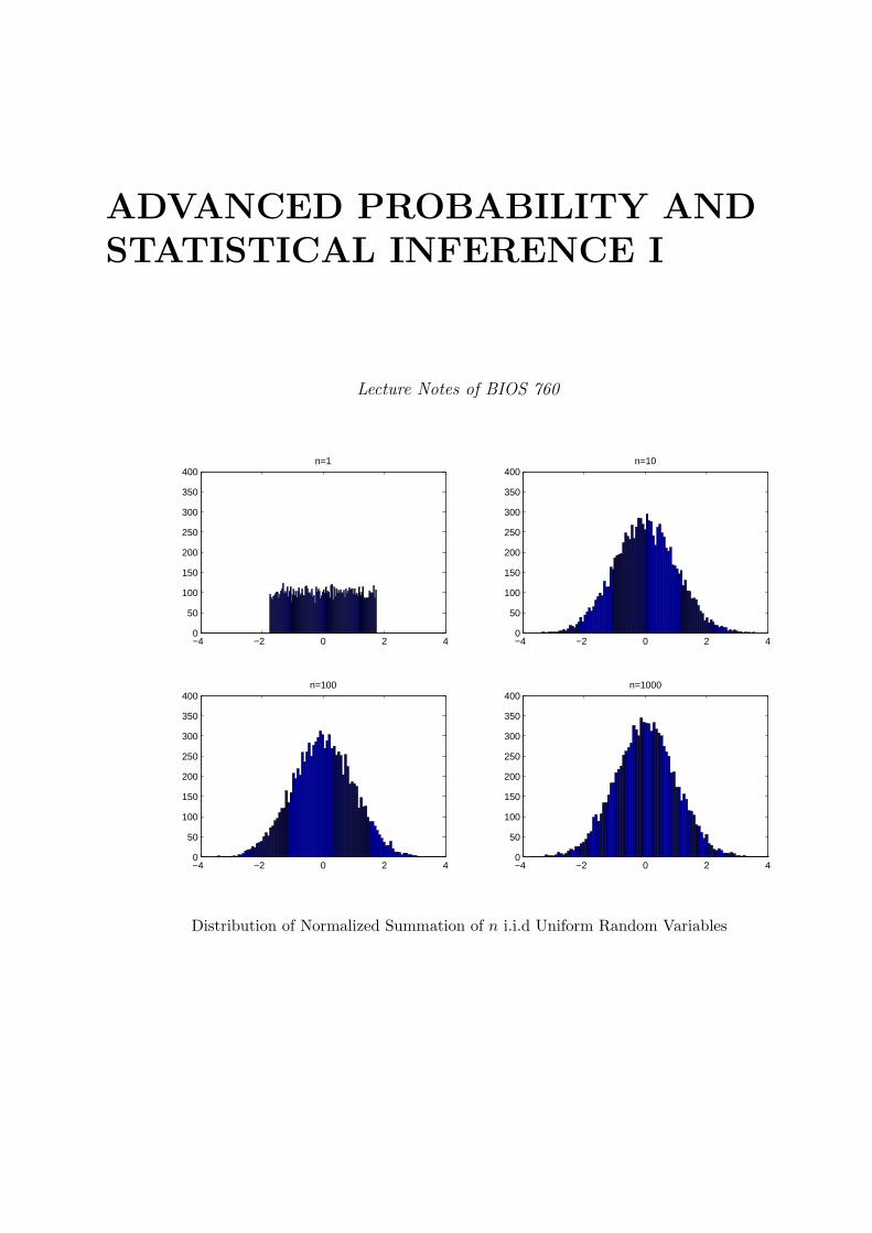
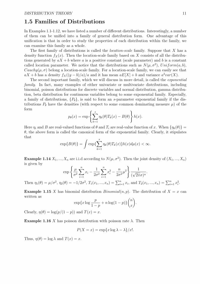
400n=1
−4 −2 0 2 40
50
100
150
200
250
300
350
400n=10
−4 −2 0 2 40
50
100
150
200
250
300
350
400n=100
−4 −2 0 2 40
50
100
150
200
250
300
350
400n=1000
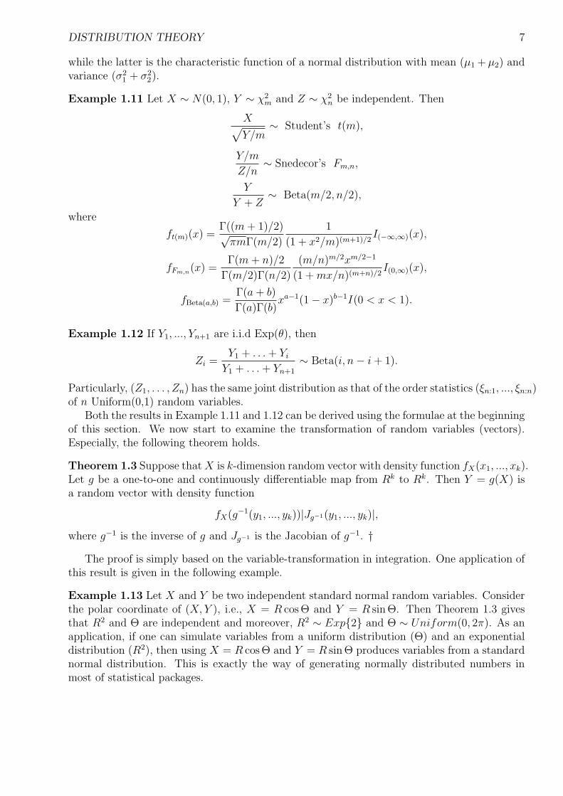
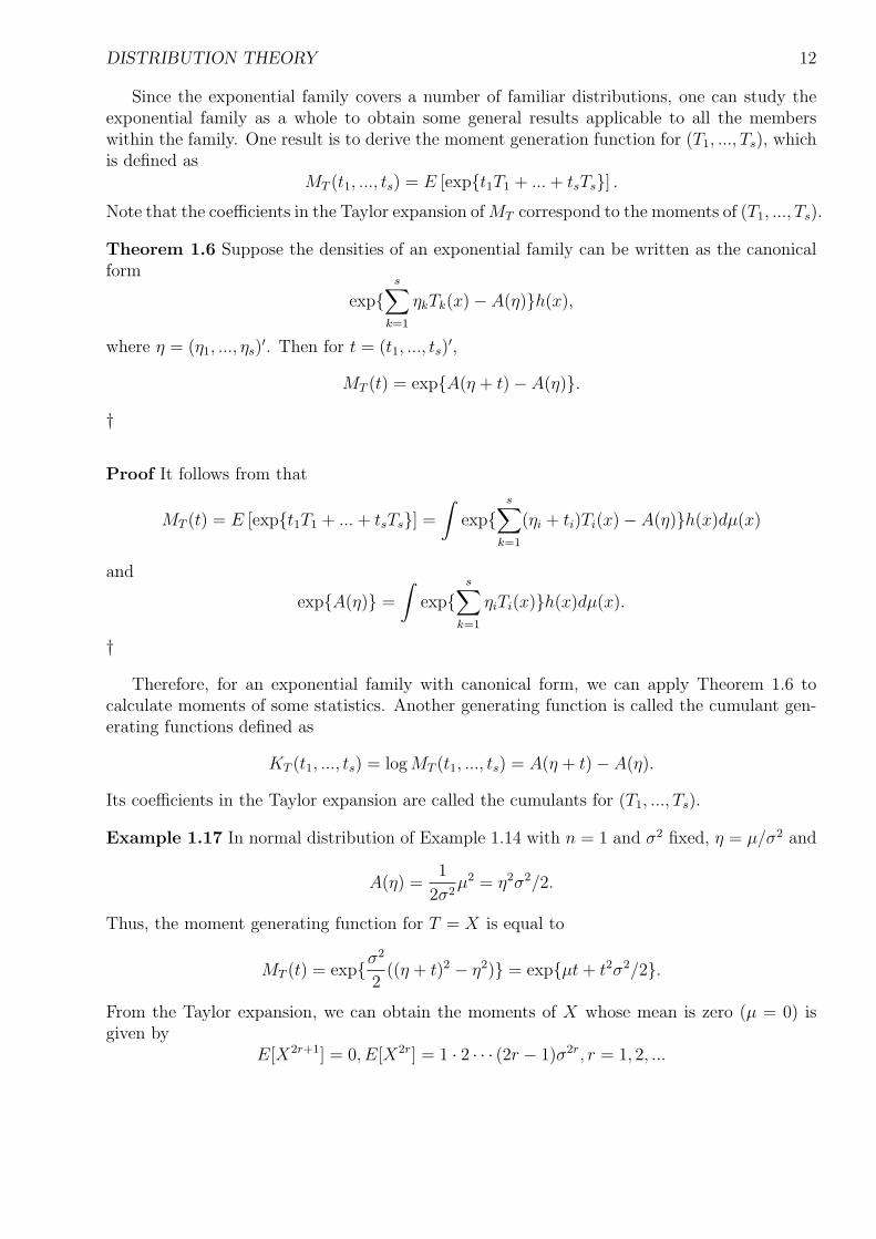
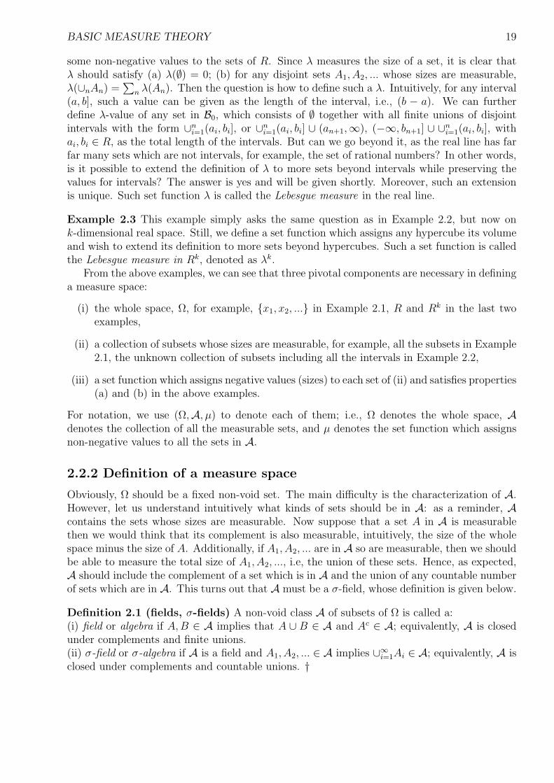
Distribution of Normalized Summation of n i.i.d Uniform Random Variables

PREFACE
These course notes have been revised based on my past teaching experience at the departmentof Biostatistics in the University of North Carolina in Fall 2004 and Fall 2005. The context in-cludes distribution theory, probability and measure theory, large sample theory, theory of pointestimation and efficiency theory. The last chapter specially focuses on maximum likelihoodapproach. Knowledge of fundamental real analysis and statistical inference will be helpful forreading these notes.
Most parts of the notes are compiled with moderate changes based on two valuable textbooks:Theory of Point Estimation (second edition, Lehmann and Casella, 1998) and A Course inLarge Sample Theory (Ferguson, 2002). Some notes are also borrowed from a similar coursetaught in the University of Washington, Seattle, by Professor Jon Wellner. The revision hasincorporated valuable comments from my colleagues and students sitting in my previous classes.However, there are inevitably numerous errors in the notes and I take all the responsibilitiesfor these errors.
Donglin ZengAugust, 2006
CHAPTER 1 A REVIEW OFDISTRIBUTION THEORY
This chapter reviews some basic concepts of discrete and continuous random variables. Distri-bution results on algebra and transformations of random variables (vectors) are given. Part ofthe chapter pays special attention to the properties of the Gaussian distributions. The finalpart of this chapter introduces some commonly-used distribution families.
1.1 Basic Concepts
Random variables are often classified into discrete random variables and continuous randomvariables. By names, discrete random variables are some variables which take discrete valueswith an associated probability mass function; while, continuous random variables are variablestaking non-discrete values (usually R) with an associated probability density function. A proba-bility mass function consists of countable non-negative values with their total sum being one anda probability density function is a non-negative function in real line with its whole integrationbeing one.
However, the above definitions are not rigorous. What is the precise definition of a randomvariable? Why shall we distinguish between mass functions or density functions? Can somerandom variable be both discrete and continuous? The answers to these questions will becomeclear in next chapter on probability measure theory. However, you may take a glimpse below:
(a) Random variables are essentially measurable functions from a probability measure spaceto real space. Especially, discrete random variables map into discrete set and continuousrandom variables map into the whole real line.
(b) Probability (probability measure) is a function assigning non-negative values to sets of aσ-field and it satisfies the property of countable additivity.
(c) Probability mass function for a discrete random variable is the Radon-Nykodym derivativeof random variable-induced measure with respect to a counting measure. Probabilitydensity function for continuous random variable is the Radon-Nykodym derivative ofrandom variable-induced measure with respect to the Lebesgue measure.
For this chapter, we do not need to worry about these abstract definitions.Some quantities to describe the distribution of a random variable include cumulative distri-
bution function, mean, variance, quantile, mode, moments, centralized moments, kurtosis andskewness. For instance, if X is a discrete random variable taking values x1, x2, ... with probabili-ties m1,m2, .... The cumulative distribution function of X is defined as FX(x) =
∑xi≤x mi. The
1
DISTRIBUTION THEORY 2
kth moment of X is given as E[Xk] =∑
i mixki and the kth centralized moment of X is given as
E[(X − µ)k] where µ is the expectation of X. If X is a continuous random variable with prob-ability density function fX(x), then the cumulative distribution function FX(x) =
∫ x
−∞ fX(t)dt
and the kth moment of X is given as E[Xk] =∫∞−∞ xkfX(x)dx if the integration is finite.
The skewness of X is given by E[(X − µ)3]/V ar(X)3/2 and the kurtosis of X is given byE[(X − µ)4]/V ar(X)2. The last two quantities describe the shape of the density function:negative values for the skewness indicate the distribution that are skewed left and positive val-ues for the skewness indicate the distribution that are skewed right. By skewed left, we meanthat the left tail is heavier than the right tail. Similarly, skewed right means that the righttail is heavier than the left tail. Large kurtosis indicates a “peaked” distribution and smallkurtosis indicates a “flat” distribution. Note that we have already used E[g(X)] to denote theexpectation of g(X). Sometimes, we use
∫g(x)dFX(x) to represent it no matter wether X is
continuous or discrete. This notation will be clear after we introduce the probability measure.Next we review an important definition in distribution theory, namely the characteris-
tic function of X. By definition, the characteristic function for X is defined as φX(t) =E[expitX ] =
∫expitxdFX (x ), where i is the imaginary unit, the square-root of -1. Equiva-
lently, φX(t) is equal to∫
expitxfX (x )dx for continuous X and is∑
j mj expitxj for discreteX. The characteristic function is important since it uniquely determines the distribution func-tion of X, the fact implied in the following theorem.
Theorem 1.1 (Uniqueness Theorem) If a random variable X with distribution functionFX has a characteristic function φX(t) and if a and b are continuous points of FX , then
FX(b)− FX(a) = limT→∞
1
2π
∫ T
−T
e−ita − e−itb
itφX(t)dt.
Moreover, if FX has a density function fX (for continuous random variable X) , then
fX(x) =1
2π
∫ ∞
−∞e−itxφX(t)dt.
†
We defer the proof to Chapter 3. Similar to the characteristic function, we can define themoment generating function for X as MX(t) = E[exptX]. However, we note that MX(t) maynot exist for some t but φX(t) always exists.
Another important and distinct feature in distribution theory is the independence of tworandom variables. For two random variables X and Y , we say X and Y are independent ifP (X ≤ x, Y ≤ y) = P (X ≤ x)P (Y ≤ y); i.e., the joint distribution function of (X,Y )is the product of the two marginal distributions. If (X, Y ) has a joint density, then anequivalent definition is that the joint density of (X,Y ) is the product of two marginal den-sities. Independence introduces many useful properties, among which one important propertyis that E[g(X)h(Y )] = E[g(X)]E[h(Y )] for any sensible functions g and h. In more gen-eral case when X and Y may not be independent, we can calculate the conditional densityof X given Y , denoted by fX|Y (x|y), as the ratio between the joint density of (X,Y ) andthe marginal density of Y . Thus, the conditional expectation of X given Y = y is equal to
DISTRIBUTION THEORY 3
E[X|Y = y] =∫
xfX|Y (x|y)dx. Clearly, when X and Y are independent, fX|Y (x|y) = fX(x)and E[X|Y = y] = E[X]. For conditional expectation, two formulae are useful:
E[X] = E[E[X|Y ]] and V ar(X) = E[V ar(X|Y )] + V ar(E[X|Y ]).
So far, we have reviewed some basic concepts for a single random variable. All the abovedefinitions can be generalized to multivariate random vector X = (X1, ..., Xk)
′ with a jointprobability mass function or a joint density function. For example, we can define the meanvector of X as E[X] = (E[X1], ..., E[Xk])
′ and define the covariance matrix for X as E[XX ′]−E[X]E[X]′. The cumulative distribution function for X is a k-variate function FX(x1, ..., xk) =P (X1 ≤ x1, ..., Xk ≤ xk) and the characteristic function of X is a k-variate function, defined as
φX(t1, ..., tk) = E[ei(t1X1+...+tkXk )] =
∫
Rk
ei(t1 x1+...+tkxk )dFX(x1, ..., xk).
Same as Theorem 1.1, an inversion formula holds: Let A = (x1, .., xk) : a1 < x1 ≤ b1, . . . , ak <xk ≤ bk be a rectangle in Rk and assume P (X ∈ ∂A) = 0, where ∂A is the boundary of A.Then
FX(b1, ..., bk)− FX(a1, ..., ak) = P (X ∈ A)
= limT→∞
1
(2π)k
∫ T
−T
· · ·∫ T
−T
k∏j=1
e−itj aj − e−itj bj
itjφX(t1, ..., tk)dt1 · · · dtk.
Finally, we can define the conditional density, the conditional expectation, the independence oftwo random vectors similar to the univariate case.
1.2 Examples of Special Distributions
We list some commonly-used distributions in the following examples.
Example 1.1 Bernoulli Distribution and Binomial Distribution A random variable Xis said to be Bernoulli(p) if P (X = 1) = p = 1 − P (X = 0). If X1, ..., Xn are independent,identically distributed (i.i.d) Bernoulli(p), then Sn = X1 + ... + Xn has a binomial distribution,denoted by Sn ∼ Binomial(n, p), with
P (Sn = k) =
(n
k
)pk(1− p)n−k.
The mean of Sn is equal to np and the variance of Sn is equal to np(1− p). The characteristicfunction for Sn is given by
E[eitSn ] = (1− p + peit)n.
Clearly, if S1 ∼ Binomial(n1, p) and S2 ∼ Binomial(n2, p) and S1, S2 are independent, thenS1 + S2 ∼ Binomial(n1 + n2, p).
Example 1.2 Geometric Distribution and Negative Binomial Distribution Let X1, X2, ...be i.i.d Bernoulli(p). Define W1 = minn : X1 + ... + Xn = 1. Then it is easy to see
P (W1 = k) = (1− p)k−1p, k = 1, 2, ...
DISTRIBUTION THEORY 4
We say W1 has a geometric distribution: W1 ∼ Geometric(p). To be general, define Wm =minn : X1 + ... + Xn = m to be the first time that m successes are obtained. Then
P (Wm = k) =
(k − 1
m− 1
)pm(1− p)k−m, k = m,m + 1, ...
Wm is said to have negative binomial distribution: Wm ∼ Negative Binomial(m, p). The meanof Wm is equal to m/p and the variance of Wm is m/p2−m/p. If Z1 ∼ Negative Binomial(m1, p)and Z2 ∼ Negative Binomial(m2, p) and Z1, Z2 are independent, then
Z1 + Z2 ∼ Negative Binomial(m1 + m2, p).
Example 1.3 Hypergeometric Distribution A hypergeometric distribution can be obtainedusing the following urn model: suppose that an urn contains N balls with M bearing the number1 and N −M bearing the number 0. We randomly draw a ball and denote its number as X1.Clearly, X1 ∼ Bernoulli(p) where p = M/N . Now replace the ball back in the urn andrandomly draw a second ball with number X2 and so forth. Let Sn = X1 + ... + Xn be the sumof all the numbers in n draws. Clearly, Sn ∼ Binomial(n, p). However, if each time we draw aball but we do not replace back, then X1, ..., Xn are dependent random variable. It is knownthat Sn has a hypergeometric distribution:
P (Sn = k) =
(Mk
)(N−Mn−k
)(
Nn
) , k = 0, 1, .., n.
Or, we write Sn ∼ Hypergeometric(N, M, n).
Example 1.4 Poisson Distribution A random variable X is said to have a Poisson distri-bution with rate λ, denoted X ∼ Poisson(λ), if
P (X = k) =λke−λ
k!, k = 0, 1, 2, ...
It is known that E[X] = V ar(X) = λ and the characteristic function for X is equal exp−λ(1−eit). Thus, if X1 ∼ Poisson(λ1) and X2 ∼ Poisson(λ2) are independent, then X1 + X2 ∼Poisson(λ1 + λ2). It is also straightforward to check that conditional on X1 + X2 = n, X1 isBinomial(n, λ1/(λ1 + λ2)). In fact, a Poisson distribution can be considered as the summationof a sequence of bernoulli trials each with small success probability: suppose that Xn1, ..., Xnn
are i.i.d Bernoulli(pn) and npn → λ. Then Sn = Xn1 + ...+Xnn has a Binomial(n, pn). We notethat for fixed k, when n is large,
P (Sn = k) =n!
k!(n− k)!pk
n(1− pn)n−k → λk
k!e−λ.
Example 1.5 Multinomial Distribution Suppose that B1, ..., Bk is a partition of R. LetY1, ..., Yn be i.i.d random variables. Let X i = (Xi1, ..., Xik) ≡ (IB1(Yi), ..., IBk
(Yi)) for i = 1, ..., n
DISTRIBUTION THEORY 5
and set N = (N1, ..., Nk) =∑n
i=1 Xi. That is, Nl, 1 ≤ l ≤ k counts the number of times thatY1, ..., Yn fall into Bl. It is easy to calculate
P (N1 = n1, ..., Nk = nk) =
(n
n1, ..., nk
)pn1
1 · · · pnkk , n1 + ... + nk = n,
where p1 = P (Y1 ∈ B1), ..., pk = P (Y1 ∈ Bk). Such a distribution is called the Multinomialdistribution, denoted Multinomial(n, (p1, .., pk)). We note that each Nl is a binomial distributionwith mean npl. Moreover, the covariance matrix for (N1, ..., Nk) is given by
n
p1(1− p1) . . . −p1pk...
. . ....
−p1pk . . . pk(1− pk)
.
Example 1.6 Uniform Distribution A random variable X has a uniform distribution in aninterval [a, b] if X’s density function is given by I[a,b](x)/(b−a), denoted by X ∼ Uniform(a, b).Moreover, E[X] = (a + b)/2 and V ar(X) = (b− a)2/12.
Example 1.7 Normal Distribution The normal distribution is the most commonly useddistribution and a random variable X with N(µ, σ2) has a probability density function
1√2πσ2
exp−(x− µ)2
2σ2.
Moreover, E[X] = µ and var(X) = σ2. The characteristic function for X is given by expitµ−σ2 t2/2. We will discuss such distribution in detail later.
Example 1.8 Gamma Distribution A Gamma distribution has a probability density
1
βθΓ(θ)xθ−1 exp−x
β, x > 0
denoted by Γ(θ, β). It has mean θβ and variance θβ2. Specially, when θ = 1, the distributionis called the exponential distribution, Exp(β). When θ = n/2 and β = 2, the distribution iscalled the Chi-square distribution with degrees of freedom n, denoted by χ2
n.
Example 1.9 Cauchy Distribution The density for a random variable X ∼ Cauchy(a, b)has the form
1
bπ 1 + (x− a)2/b2 .
Note E[X] = ∞. Such a distribution is often used as a counterexample in distribution theory.Many other distributions can be constructed using some elementary algebra such as sum-
mation, product, quotient of the above special distributions. We will discuss them in nextsection.
DISTRIBUTION THEORY 6
1.3 Algebra and Transformation of Random Variables (Vec-
tors)
In many applications, one wishes to calculate the distribution of some algebraic expressionof independent random variables. For example, suppose that X and Y are two independentrandom variables. We wish to find the distributions of X +Y , XY and X/Y (we assume Y > 0for the last two cases).
The calculation of these algebraic distributions is often done using the conditional expec-tation. To see how this works, we denote FZ(·) as the cumulative distribution function of anyrandom variable Z. Then for X + Y ,
FX+Y (z) = E[I(X+Y ≤ z)] = EY [EX [I(X ≤ z−Y )|Y ]] = EY [FX(z−Y )] =
∫FX(z−y)dFY (y);
symmetrically,
FX+Y (z) =
∫FY (z − x)dFX(x).
The above formula is called the convolution formula, sometimes denoted by FX ∗FY (z). If bothX and Y have densities functions fX and fY respectively, then the density function for X + Yis equal to
fX ∗ fY (z) ≡∫
fX(z − y)fY (y)dy =
∫fY (z − x)fX(x)dx.
Similarly, we can obtain the formulae for XY and X/Y as follows:
FXY (z) = E[E[I(XY ≤ z)|Y ]] =
∫FX(z/y)dFY (y), fXY (z) =
∫fX(z/y)/yfY (y)dy,
FX/Y (z) = E[E[I(X/Y ≤ z)|Y ]] =
∫FX(yz)dFY (y), fX/Y (z) =
∫fX(yz)yfY (y)dy.
These formulae can be used to construct some familiar distributions from simple randomvariables. We assume X and Y are independent in the following examples.
Example 1.10 (i) X ∼ N(µ1, σ21) and Y ∼ N(µ2, σ
22). X + Y ∼ N(µ1 + µ2, σ
21 + σ2
2).(ii) X ∼ Cauchy(0, σ1) and Y ∼ Cauchy(0, σ2) implies X + Y ∼ Cauchy(0, σ1 + σ2).(iii) X ∼ Gamma(r1, θ) and Y ∼ Gamma(r2, θ) implies that X + Y ∼ Gamma(r1 + r2, θ).(iv) X ∼ Poisson(λ1) and Y ∼ Poisson(λ2) implies X + Y ∼ Poisson(λ1 + λ2).(v) X ∼ Negative Binomial(m1, p) and Y ∼ Negative Binomial(m2, p). Then X +Y ∼ NegativeBinomial(m1 + m2, p).
The results in Example 1.10 can be verified using the convolution formula. However, theseresults can also be obtained using characteristic functions, as stated in the following theorem.
Theorem 1.2 Let φX(t) denote the characteristic function for X. Suppose X and Y areindependent. Then φX+Y (t) = φX(t)φY (t). †
The proof is direct. We can use Theorem 1.2 to find the distribution of X +Y . For example,in (i) of Example 1.10, we know φX(t) = expµ1t − σ2
1t2/2 and φY (t) = expµ2t − σ2
2t2/2.
Thus,φX+Y (t) = exp(µ1 + µ2)t− (σ2
1 + σ22)t
2/;
DISTRIBUTION THEORY 7
while the latter is the characteristic function of a normal distribution with mean (µ1 + µ2) andvariance (σ2
1 + σ22).
Example 1.11 Let X ∼ N(0, 1), Y ∼ χ2m and Z ∼ χ2
n be independent. Then
X√Y/m
∼ Student’s t(m),
Y/m
Z/n∼ Snedecor’s Fm,n,
Y
Y + Z∼ Beta(m/2, n/2),
where
ft(m)(x) =Γ((m + 1)/2)√
πmΓ(m/2)
1
(1 + x2/m)(m+1)/2I(−∞,∞)(x),
fFm,n(x) =Γ(m + n)/2
Γ(m/2)Γ(n/2)
(m/n)m/2xm/2−1
(1 + mx/n)(m+n)/2I(0,∞)(x),
fBeta(a,b) =Γ(a + b)
Γ(a)Γ(b)xa−1(1− x)b−1I(0 < x < 1).
Example 1.12 If Y1, ..., Yn+1 are i.i.d Exp(θ), then
Zi =Y1 + . . . + Yi
Y1 + . . . + Yn+1
∼ Beta(i, n− i + 1).
Particularly, (Z1, . . . , Zn) has the same joint distribution as that of the order statistics (ξn:1, ..., ξn:n)of n Uniform(0,1) random variables.
Both the results in Example 1.11 and 1.12 can be derived using the formulae at the beginningof this section. We now start to examine the transformation of random variables (vectors).Especially, the following theorem holds.
Theorem 1.3 Suppose that X is k-dimension random vector with density function fX(x1, ..., xk).Let g be a one-to-one and continuously differentiable map from Rk to Rk. Then Y = g(X) isa random vector with density function
fX(g−1(y1, ..., yk))|Jg−1(y1, ..., yk)|,where g−1 is the inverse of g and Jg−1 is the Jacobian of g−1. †
The proof is simply based on the variable-transformation in integration. One application ofthis result is given in the following example.
Example 1.13 Let X and Y be two independent standard normal random variables. Considerthe polar coordinate of (X, Y ), i.e., X = R cos Θ and Y = R sin Θ. Then Theorem 1.3 givesthat R2 and Θ are independent and moreover, R2 ∼ Exp2 and Θ ∼ Uniform(0, 2π). As anapplication, if one can simulate variables from a uniform distribution (Θ) and an exponentialdistribution (R2), then using X = R cos Θ and Y = R sin Θ produces variables from a standardnormal distribution. This is exactly the way of generating normally distributed numbers inmost of statistical packages.
DISTRIBUTION THEORY 8
1.4 Multivariate Normal Distribution
One particular distribution we will encounter in larger-sample theory is the multivariate normaldistribution. A random vector Y = (Y1, ..., Yn)′ is said to have a multivariate normal distributionwith mean vector µ = (µ1, ..., µn)′ and non-degenerate covariance matrix Σn×n, denoted asN(µ, Σ) or Nn(µ, Σ) to emphasize Y ’s dimension, if Y has a joint density as
fY (y1, ..., yn) =1
(2π)n/2|Σ|1/2exp−1
2(y − µ)′Σ−1(y − µ).
We can derive the characteristic function of Y using the following ad hoc way:
φY (t) = E[eit′Y ]
=1
(2π)n/2|Σ|1/2
∫expit′y − 1
2(y − µ)′Σ−1(y − µ)dy
=1
(2π)n/2|Σ|1/2
∫exp−1
2y′Σ−1y + (it + Σ−1µ)′y − µ′Σ−1µ
2dy
=exp−µ′Σ−1µ/2
(2π)n/2|Σ|1/2
∫exp
−1
2(y − Σit− µ)′Σ−1(y − Σit− µ)
+1
2(Σit + µ)′Σ−1(Σit + µ)
dy
= expit′µ− 1
2t′Σt.
Particularly, if Y has standard multivariate normal distribution with mean zero and covarianceIn×n, φY (t) = exp−t′t/2.
The following theorem describes the properties of a multivariate normal distribution.
Theorem 1.4 If Y = An×kXk×1 where X ∼ Nk(0, I) (standard multivariate normal distribu-tion), then Y ’s characteristic function is given by
φY (t) = exp −t′Σt/2 , t = (t1, ..., tn) ∈ Rk
and rank(Σ) = rank(A). Conversely, if φY (t) = exp−t′Σt/2 with Σn×n ≥ 0 of rank k, then
Y = An×kXk×1 with rank(A) = k and X ∼ Nk(0, I).
†
Proof
φY (t) = E[expit′(AX)] = E[expi(A′t)′X] = exp−(A′t)′(A′t)/2 = exp−t′AA′t/2.
Thus, Σ = AA′ and rank(Σ) = rank(A). Conversely, if φY (t) = exp−t′Σt/2, then frommatrix theory, there exist an orthogonal matrix O such that Σ = O′DO, where D is a diagonalmatrix with first k diagonal elements positive and the rest (n− k) elements being zero. Denote
DISTRIBUTION THEORY 9
these positive diagonal elements as d1, ..., dk. Define Z = OY . Then the characteristic functionfor Z is given by
φZ(t) = E[expit ′(OY )] = E [expi(O ′t)′Y ] = exp−(O ′t)′Σ (O ′t)/2
= exp−d1t21/2− ...− dkt
2k/2.
This implies that Z1, ..., Zk are independent N(0, d1), ..., N(0, dk) and Zk+1 = ... = Zn = 0. LetXi = Zi/
√di for i = 1, ..., k and write O′ = (Bn×k, Cn×(n−k)). Then
Y = O′Z = Bn×k
Z1...
Zk
= Bn×kdiag(
√d1, ...,
√dk)
X1...
Xk
≡ AX.
Clearly, rank(A) = k. †
Theorem 1.5 Suppose that Y = (Y1, ..., Yk, Yk+1, ..., Yn)′ has a multivariate normal distribution
with mean µ = (µ(1)′, µ(2)′)′ and a non-degenerate covariance matrix
Σ =
(Σ11 Σ12
Σ21 Σ22
).
Then(i) (Y1, ..., Yk)
′ ∼ Nk(µ(1), Σ11).
(ii) (Y1, ..., Yk)′ and (Yk+1, ..., Yn)′ are independent if and only if Σ12 = Σ21 = 0.
(iii) For any matrix Am×n, AY has a multivariate normal distribution with mean Aµ and co-variance AΣA′.(iv) The conditional distribution of Y (1) = (Y1, ..., Yk)
′ given Y (2) = (Yk+1, ..., Yn)′ is a multi-variate normal distribution given as
Y (1)|Y (2) ∼ Nk(µ(1) + Σ12Σ
−122 (Y (2) − µ(2)), Σ11 − Σ12Σ
−122 Σ21).
†
Proof (i) From Theorem 1.4, we obtain that the characteristic function for (Y1, ..., Yk) − µ(1)
is given by exp−t′(DΣ)(DΣ)′t/2, where D = (Ik×k 0k×(n−k)). Thus, the characteristicfunction is equal to
exp −(t1, ..., tk)Σ11(t1, ..., tk)′/2 ,
which is the same as the characteristic function from Nk(0, Σ11).(ii) The characteristics function for Y can be written as
exp
[it(1)′µ(1) + it(2)′µ(2) − 1
2
t(1)′Σ11t
(1) + 2t(1)′Σ12t(2) + t(2)′Σ22t
(2)]
.
If Σ12 = 0, the characteristics function can be factorized as the product of the separate functionsfor t(1) and t(2). Thus, Y (1) and Y (2) are independent. The converse is obviously true.(iii) The result follows from Theorem 1.4.
DISTRIBUTION THEORY 10
(iv) Consider Z(1) = Y (1)−µ(1)−Σ12Σ−122 (Y (2)−µ(2)). From (iii), Z(1) has a multivariate normal
distribution with mean zero and covariance calculated by
Cov(Z(1), Z(1)) = Cov(Y (1), Y (1))− 2Σ12Σ−122 Cov(Y (2), Y (1)) + Σ12Σ
−122 Cov(Y (2), Y (2))Σ−1
22 Σ21
= Σ11 − Σ12Σ−122 Σ21.
On the other hand,
Cov(Z(1), Y (2)) = Cov(Y (1), Y (2))− Σ12Σ−122 Cov(Y (2), Y (2)) = 0.
From (ii), Z(1) is independent of Y (2). Then the conditional distribution Z(1) given Y (2) is thesame as the unconditional distribution of Z(1); i.e.,
Z(1)|Y (2) ∼ N(0, Σ11 − Σ12Σ−122 Σ21).
The result follows. †
With normal random variables, we can use algebra of random variables to construct anumber of useful distributions. The first one is Chi-square distribution. Suppose X ∼ Nn(0, I),then ‖X‖2 =
∑ni=1 X2
i ∼ χ2n, the chi-square distribution with n degrees of freedom. One can
use the convolution formula to obtain that the density function for χ2n is equal to the density
for the Gamma(n/2, 2), denoted by g(y; n/2, 1/2).
Corollary 1.1 If Y ∼ Nn(0, Σ) with Σ > 0, then Y ′Σ−1Y ∼ χ2n. †
Proof Since Σ > 0, there exists a positive definite matrix A such that AA′ = Σ. ThenX = A−1Y ∼ Nn(0, I). Thus
Y ′Σ−1Y = X ′X ∼ χ2n.
†
Suppose X ∼ N(µ, 1). Define Y = X2, δ = µ2. Then Y has density
fY (y) =∞∑
k=0
pk(δ/2)g(y; (2k + 1)/2, 1/2),
where pk(δ/2) = exp(−δ/2)(δ/2)k/k!. Another ways to obtain this is: Y |K = k ∼ χ22k+1
where K ∼ Poisson(δ/2). We call Y has the noncentral chi-square distribution with 1 degreeof freedom and noncentrality parameter δ and write Y ∼ χ2
1(δ). More generally, if X =(X1, ..., Xn)′ ∼ Nn(µ, I) and let Y = X ′X, then Y has a density fY (y) =
∑∞k=0 pk(δ/2)g(y; (2k+
n)/2, 1/2) where δ = µ′µ. We write Y ∼ χ2n(δ) and call Y has the noncentral chi-square
distribution with n degrees of freedom and noncentrality parameters δ. It is then easy to showthat if X ∼ N(µ, Σ), then Y = X ′Σ−1X ∼ χ2
n(δ).If X ∼ N(0, 1), Y ∼ χ2
n and they are independent, then X/√
Y/n is called t-distributionwith n degrees of freedom. If Y1 ∼ χ2
m, Y2 ∼ χ2n and Y1 and Y2 are independent, then
(Y1/m)/(Y2/m) is called F-distribution with degrees freedom of m and n. These distributionshave already been introduced in Example 1.11.
DISTRIBUTION THEORY 11
1.5 Families of Distributions
In Examples 1.1-1.12, we have listed a number of different distributions. Interestingly, a numberof them can be unified into a family of general distribution form. One advantage of thisunification is that in order to study the properties of each distribution within the family, wecan examine this family as a whole.
The first family of distributions is called the location-scale family. Suppose that X has adensity function fX(x). Then the location-scale family based on X consists of all the distribu-tions generated by aX + b where a is a positive constant (scale parameter) and b is a constantcalled location parameter. We notice that the distributions such as N(µ, σ2), Uniform(a, b),Cauchy(µ, σ) belong a location-scale family. For a location-scale family, we can easily see thataX + b has a density fX((y − b)/a)/a and it has mean aE[X] + b and variance a2var(X).
The second important family, which we will discuss in more detail, is called the exponentialfamily. In fact, many examples of either univariate or multivariate distributions, includingbinomial, poisson distributions for discrete variables and normal distribution, gamma distribu-tion, beta distribution for continuous variables belong to some exponential family. Especially,a family of distributions, Pθ, is said to form an s-parameter exponential family if the dis-tributions Pθ have the densities (with respect to some common dominating measure µ) of theform
pθ(x) = exp
s∑
k=1
ηk(θ)Tk(x)−B(θ)
h(x).
Here ηi and B are real-valued functions of θ and Ti are real-value function of x. When ηk(θ) =θ, the above form is called the canonical form of the exponential family. Clearly, it stipulatesthat
expB(θ) =
∫exp
s∑
k=1
ηk(θ)Tk(x)h(x)dµ(x) < ∞.
Example 1.14 X1, ..., Xn are i.i.d according to N(µ, σ2). Then the joint density of (X1, ..., Xn)is given by
exp
µ
σ2
n∑i=1
xi − 1
2σ2
n∑i=1
x2i −
n
2σ2µ2
1
(√
2πσ)n.
Then η1(θ) = µ/σ2, η2(θ) = −1/2σ2, T1(x1, ..., xn) =∑n
i=1 xi, and T2(x1, ..., xn) =∑n
i=1 x2i .
Example 1.15 X has binomial distribution Binomial(n, p). The distribution of X = x canwritten as
expx logp
1− p+ n log(1− p)
(n
x
).
Clearly, η(θ) = log(p/(1− p)) and T (x) = x.
Example 1.16 X has poisson distribution with poisson rate λ. Then
P (X = x) = expx log λ− λ/x!.
Thus, η(θ) = log λ and T (x) = x.
DISTRIBUTION THEORY 12
Since the exponential family covers a number of familiar distributions, one can study theexponential family as a whole to obtain some general results applicable to all the memberswithin the family. One result is to derive the moment generation function for (T1, ..., Ts), whichis defined as
MT (t1, ..., ts) = E [expt1T1 + ... + tsTs] .Note that the coefficients in the Taylor expansion of MT correspond to the moments of (T1, ..., Ts).
Theorem 1.6 Suppose the densities of an exponential family can be written as the canonicalform
exps∑
k=1
ηkTk(x)− A(η)h(x),
where η = (η1, ..., ηs)′. Then for t = (t1, ..., ts)
′,
MT (t) = expA(η + t)− A(η).†
Proof It follows from that
MT (t) = E [expt1T1 + ... + tsTs] =
∫exp
s∑
k=1
(ηi + ti)Ti(x)− A(η)h(x)dµ(x)
and
expA(η) =
∫exp
s∑
k=1
ηiTi(x)h(x)dµ(x).
†
Therefore, for an exponential family with canonical form, we can apply Theorem 1.6 tocalculate moments of some statistics. Another generating function is called the cumulant gen-erating functions defined as
KT (t1, ..., ts) = log MT (t1, ..., ts) = A(η + t)− A(η).
Its coefficients in the Taylor expansion are called the cumulants for (T1, ..., Ts).
Example 1.17 In normal distribution of Example 1.14 with n = 1 and σ2 fixed, η = µ/σ2 and
A(η) =1
2σ2µ2 = η2σ2/2.
Thus, the moment generating function for T = X is equal to
MT (t) = expσ2
2((η + t)2 − η2) = expµt + t2σ2/2.
From the Taylor expansion, we can obtain the moments of X whose mean is zero (µ = 0) isgiven by
E[X2r+1] = 0, E[X2r] = 1 · 2 · · · (2r − 1)σ2r, r = 1, 2, ...
DISTRIBUTION THEORY 13
Example 1.18 X has a gamma distribution with density
1
Γ(a)baxa−1e−x/b, x > 0.
For fixed a, it has a canonical form
exp−x/b + (a− 1) log x− log(Γ(a)ba)I(x > 0).
Correspondingly, η = −1/b, T = X, A(η) = log(Γ(a)ba) = a log(−1/η) + log Γ(a). Then themoment generating function for T = X is given by
MX(t) = expa logη
η + t = (1− bt)−a.
After the Taylor expansion around zero, we obtain
E[X] = ab, E[X2] = ab2 + (ab)2, ...
As a further note, the exponential family has an important role in classical statistical infer-ence since it possesses many nice statistical properties. We will revisit it in Chapter 4.
READING MATERIALS : You should read Lehmann and Casella, Sections 1.4 and 1.5.
PROBLEMS
1. Verify the densities of t(m) and Fm,n in Example 1.11.
2. Verify the two results in Example 1.12.
3. Suppose X ∼ N(ν, 1). Show that Y = X2 has a density
fY (y) =∞∑
k=0
pk(µ2/2)g(y; (2k + 1)/2, 1/2),
where pk(µ2/2) = exp(−µ2/2)(µ2/2)k/k! and g(y; n/2, 1/2) is the density of Gamma(n/2, 2).
4. Suppose X = (X1, ..., Xn) ∼ N(µ, I) and let Y = X ′X. Show that Y has a density
fY (y) =∞∑
k=0
pk(µ′µ/2)g(y; (2k + n)/2, 1/2).
5. Let X ∼ Gamma(α1, β) and Y ∼ Gamma(α2, β) be independent random variables.Derive the distribution of X/(X + Y ).
DISTRIBUTION THEORY 14
6. Show that for any random variables X, Y and Z,
Cov(X, Y ) = E[Cov(X, Y |Z)] + Cov(E[X|Z], E[Y |Z]),
where Cov(X,Y |Z) is the conditional covariance of X and Y given Z.
7. Let X and Y be i.i.d Uniform(0,1) random variables. Define U = X−Y , V = max(X, Y ) =X ∨ Y .
(a) What is the range of (U, V )?
(b) find the joint density function fU,V (u, v) of the pair (U, V ). Are U and V indepen-dent?
8. Suppose that for θ ∈ R,
fθ(u, v) = 1 + θ(1− 2u)(1− 2v) I(0 ≤ u ≤ 1, 0 ≤ v ≤ 1).
(a) For what values of θ is fθ a density function in [0, 1]2?
(b) For the set of θ’s identified in (a), find the corresponding distribution function Fθ
and show that it has Uniform(0,1) marginal distributions.
(c) If (U, V ) ∼ fθ, compute the correlation ρ(U, V ) ≡ ρ as a function of θ.
9. Suppose that F is the distribution function of random variables X and Y with X ∼Uniform(0, 1) marginally and Y ∼ Uniform(0, 1) marginally. Thus, F (x, y) satisfies
F (x, 1) = x, 0 ≤ x ≤ 1, and F (1, y) = y, 0 ≤ y ≤ 1.
(a) Show thatF (x, y) ≤ x ∧ y
for all 0 ≤ x ≤ 1, 0 ≤ y ≤ 1. Here x ∧ y = min(x, y) and we denote it as FU(x, y).
(b) Show thatF (x, y) ≥ (x + y − 1)+
for all 0 ≤ x ≤ 1, 0 ≤ y ≤ 1. Here (x + y − 1)+ = max(x + y − 1, 0) and we denoteit as FL(x, y).
(c) Show that FU is the distribution function of (X, X) and FL is the distribution func-tion of (X, 1−X).
10. (a) If W ∼ χ22 = Gamma(1, 2), find the density of W , the distribution function W and
the inverse distribution function explicitly.
(b) Suppose that (X, Y ) ∼ N(0, I2×2). In two-dimensional plane, let R be the distanceof (X, Y ) from (0, 0) and θ be the angle between the line from (0,0) to (X,Y) andthe right-half line of x-axis. Then X = R cos Θ and Y = R sin Θ. Show that R andΘ are independent random variables with R2 ∼ χ2
2 and Θ ∼ Uniform(0, 2π).
(c) Use the above two results to show how to use two independent Uniform(0,1) randomvariables U and V to generate two standard normal random variables. Hint: use oneresult that if X has a distribution function F then F (X) has a uniform distributionin [0, 1].
DISTRIBUTION THEORY 15
11. Suppose that X ∼ F on [0,∞), Y ∼ G on [0,∞), and X and Y are independent randomvariables. Let Z = minX, Y = X ∧ Y and ∆ = I(X ≤ Y ).
(a) Find the joint distribution of (Z, ∆).
(b) If X ∼ Exponential(λ) and Y ∼ Exponential(µ), show that Z and ∆ are indepen-dent.
12. Let X1, ..., Xn be i.i.d N(0, σ2). (w1, ..., wn) is a constant vector such that w1, ..., wn > 0and w1 + ... + wn = 1. Define Xnw =
√w1X1 + ... +
√wnXn. Show that
(a) Yn = Xnw/σ ∼ N(0, 1).
(b) (n− 1)S2n/σ
2 = (∑n
i=1 X2i − X2
nw)/σ2 ∼ χ2n−1.
(c) Yn and S2n are independent so Tn = Yn/
√S2
n ∼ tn−1/σ.
(d) when w1 = ... = wn = 1/n, show that Yn is the standardized sample mean and S2n is
the sample variance.
Hint: Consider an orthogonal matrix Σ such that the first row is (√
w1, ...,√
wn). Let
Z1...
Zn
= Σ
X1...
Xn
.
Then Yn = Z1/σ and (n− 1)S2n/σ2 = (Z2
2 + ... + Z2n)/σ2.
13. Let Xn×1 ∼ N(0, In×n). Suppose that A is a symmetric matrix with rank r. ThenX ′AX ∼ χ2
r if and only if A is a projection matrix (that is, A2 = A). Hint: use thefollowing result from linear algebra: for any symmetric matrix, there exits an orthogonalmatrix O such that A = O′ diag((d1, ..., dn))O; A is a projection matrix if and only ifd1, ..., dn take values of 0 or 1’s.
14. Let Wm ∼ Negative Binomial(m, p). Consider p as a parameter.
(a) Write the distribution as an exponential family.
(b) Use the result for the exponential family to derive the moment generating functionof Wm, denoted by M(t).
(c) Calculate the first and the second cumulants of Wm. By definition, in the expansionof the cumulant generating function,
log M(t) =∞∑
k=0
µk
k!tk,
µk is the kth cumulant of Wm. Note that these two cumulants are exactly the meanand the variance of Wm.
15. For the density C exp−|x|1/2
,−∞ < x < ∞, where C is the normalized constant,
show that moments of all orders exist but the moment generating function exists only att = 0.

DISTRIBUTION THEORY 16
16. Lehmann and Casella, page 64, problem 4.2.
17. Lehmann and Casella, page 66, problem 5.6.
18. Lehmann and Casella, page 66, problem 5.7.
19. Lehmann and Casella, page 66, problem 5.8.
20. Lehmann and Casella, page 66, problem 5.9.
21. Lehmann and Casella, page 66, problem 5.10.
22. Lehmann and Casella, page 67, problem 5.12.
23. Lehmann and Casella, page 67, problem 5.14.
CHAPTER 2 MEASURE,INTEGRATION ANDPROBABILITY
This chapter is an introduction to (probability) measure theories, a foundation for all theprobabilistic and statistical framework. We first give the definition of a measure space. Thenwe introduce measurable functions in a measure space and the integration and convergence ofmeasurable functions. Further generalization including the product of two measures and theRadon-Nikodym derivatives of two measures is introduced. As a special case, we describe howthe concepts and the properties in measure space are used in parallel in a probability measurespace.
2.1 A Review of Set Theory and Topology in Real Space
We review some basic concepts in set theory. A set is a collection of elements, which can be acollection of real numbers, a group of abstract subjects and etc. In most of cases, we considerthat these elements come from one largest set, called a whole space. By custom, a whole spaceis denoted by Ω so any set is simply a subset of Ω. We can exhaust all possible subsets of Ωthen the collection of all these subsets is denoted as 2Ω, called the power set of Ω. We alsoinclude the empty set, which has no element at all and is denoted by ∅, in this power set.
For any two subsets A and B of the whole space Ω, A is said to be a subset of B if B containsall the elements of A, denoted as A ⊆ B. For arbitrary number of sets Aα : α is some index,where the index of α can be finite, countable or uncountable, we define the intersection of thesesets as the set which contains all the elements common to Aα for any α. The intersection ofthese sets is denoted as ∩αAα. Aα’s are disjoint if any two sets have empty intersection. Wecan also define the union of these sets as the set which contains all the elements belonging toat least one of these sets, denoted as ∪αAα. Finally, we introduce the complement of a set A,denoted by Ac, to be the set which contains all the elements not in A. Among the definitionsof set intersection, union and complement, the following relationships are clear: for any B andAα,
B ∩ ∪αAα = ∪α B ∩ Aα , B ∪ ∩αAα = ∩α B ∪ Aα ,
∪αAαc = ∩αAcα, ∩αAαc = ∪αAc
α. ( de Morgan law)
Sometimes, we use (A − B) to denote a subset of A excluding any elements in B. Thus(A − B) = A ∩ Bc. Using this notation, we can always partition the union of any countable
17
BASIC MEASURE THEORY 18
sets A1, A2, ... into a union of countable disjoint sets:
A1 ∪ A2 ∪ A3 ∪ ... = A1 ∪ (A2 − A1) ∪ (A3 − A1 ∪ A2) ∪ ...
For a sequence of sets A1, A2, A3, ..., we now define the limit sets of the sequence. The upperlimit set of the sequence is the set which contains the elements belonging to infinite numberof the sets in this sequence; the lower limit set of the sequence is the set which contains theelements belonging to all the sets except a finite number of them in this sequence. The formeris denoted by limnAn or lim supn An and the latter is written as limnAn or lim infn An. We canshow
lim supn
An = ∩∞n=1 ∪∞m=nAm , lim infn
An = ∪∞n=1 ∩∞m=nAm .
When both limit sets agree, we say that the sequence has a limit set. In the calculus, we knowthat for any sequence of real numbers x1, x2, ..., it has a upper limit, lim supn xn, and a lowerlimit, lim infn xn, where the former refers to the upper bound of the limits for any convergentsubsequences and the latter is the lower bound. It should be cautious that such upper limit orlower limit is different from the upper limit or lower limit of sets.
The second part of this section reviews some basic topology in a real line. Because thedistance between any two points is well defined in a real line, we can define a topology in a realline. A set A of the real line is called an open set if for any point x ∈ A, there exists an openinterval (x−ε, x+ε) contained in A. Clearly, any open interval (a, b) where a could be −∞ andb could be ∞, is an open set. Moreover, for any number of open sets Aα where α is an index,it is easy to show that ∪αAα is open. A closed set is defined as the complement of an open set.It can also be show that A is closed if and only if for any sequence xn in A such that xn → x,x must belong to A. By the de Morgan law, we also see that the intersection of any numberof closed sets is still closed. Only ∅ and the whole real line are both open set and closed set;there are many sets neither open or closed, for example, the set of all the rational numbers. Ifa closed set A is bounded, A is also called a compact set. These basic topological concepts willbe used later. Note that the concepts of open set or closed set can be easily generalized to anyfinite dimensional real space.
2.2 Measure Space
2.2.1 Introduction
Before we introduce a formal definition of measure space, let us examine the following examples.
Example 2.1 Suppose that a whole space Ω contains countable number of distinct pointsx1, x2, .... For any subset A of Ω, we define a set function µ#(A) as the number of points inA. Therefore, if A has n distinct points, µ#(A) = n; if A has infinite many number of points,then µ#(A) = ∞. We can easily show that (a) µ#(∅) = 0; (b) if A1, A2, ... are disjoint sets ofΩ, then µ#(∪nAn) =
∑n µ#(An). We will see later that µ# is a measure called the counting
measure in Ω.
Example 2.2 Suppose that the whole space Ω = R, the real line. We wish to measure the sizesof any possible subsets in R. Equivalently, we wish to define a set function λ which assigns
BASIC MEASURE THEORY 19
some non-negative values to the sets of R. Since λ measures the size of a set, it is clear thatλ should satisfy (a) λ(∅) = 0; (b) for any disjoint sets A1, A2, ... whose sizes are measurable,λ(∪nAn) =
∑n λ(An). Then the question is how to define such a λ. Intuitively, for any interval
(a, b], such a value can be given as the length of the interval, i.e., (b − a). We can furtherdefine λ-value of any set in B0, which consists of ∅ together with all finite unions of disjointintervals with the form ∪n
i=1(ai, bi], or ∪ni=1(ai, bi] ∪ (an+1,∞), (−∞, bn+1] ∪ ∪n
i=1(ai, bi], withai, bi ∈ R, as the total length of the intervals. But can we go beyond it, as the real line has farfar many sets which are not intervals, for example, the set of rational numbers? In other words,is it possible to extend the definition of λ to more sets beyond intervals while preserving thevalues for intervals? The answer is yes and will be given shortly. Moreover, such an extensionis unique. Such set function λ is called the Lebesgue measure in the real line.
Example 2.3 This example simply asks the same question as in Example 2.2, but now onk-dimensional real space. Still, we define a set function which assigns any hypercube its volumeand wish to extend its definition to more sets beyond hypercubes. Such a set function is calledthe Lebesgue measure in Rk, denoted as λk.
From the above examples, we can see that three pivotal components are necessary in defininga measure space:
(i) the whole space, Ω, for example, x1, x2, ... in Example 2.1, R and Rk in the last twoexamples,
(ii) a collection of subsets whose sizes are measurable, for example, all the subsets in Example2.1, the unknown collection of subsets including all the intervals in Example 2.2,
(iii) a set function which assigns negative values (sizes) to each set of (ii) and satisfies properties(a) and (b) in the above examples.
For notation, we use (Ω,A, µ) to denote each of them; i.e., Ω denotes the whole space, Adenotes the collection of all the measurable sets, and µ denotes the set function which assignsnon-negative values to all the sets in A.
2.2.2 Definition of a measure space
Obviously, Ω should be a fixed non-void set. The main difficulty is the characterization of A.However, let us understand intuitively what kinds of sets should be in A: as a reminder, Acontains the sets whose sizes are measurable. Now suppose that a set A in A is measurablethen we would think that its complement is also measurable, intuitively, the size of the wholespace minus the size of A. Additionally, if A1, A2, ... are in A so are measurable, then we shouldbe able to measure the total size of A1, A2, ..., i.e, the union of these sets. Hence, as expected,A should include the complement of a set which is in A and the union of any countable numberof sets which are in A. This turns out that A must be a σ-field, whose definition is given below.
Definition 2.1 (fields, σ-fields) A non-void class A of subsets of Ω is called a:(i) field or algebra if A,B ∈ A implies that A ∪ B ∈ A and Ac ∈ A; equivalently, A is closedunder complements and finite unions.(ii) σ-field or σ-algebra if A is a field and A1, A2, ... ∈ A implies ∪∞i=1Ai ∈ A; equivalently, A isclosed under complements and countable unions. †
BASIC MEASURE THEORY 20
In fact, a σ-field is not only closed under complement and countable union but also closedunder countable intersection, as shown in the following proposition.
Proposition 2.1. (i) For a field A, ∅, Ω ∈ A and if A1, ..., An ∈ A, ∩ni=1Ai ∈ A.
(ii) For a σ-field A, if A1, A2, ... ∈ A, then ∩∞i=1Ai ∈ A. †
Proof (i) For any A ∈ A, Ω = A ∪ Ac ∈ A. Thus, ∅ = Ωc ∈ A. If A1, ..., An ∈ A then∩n
i=1Ai = (∪ni=1A
ci)
c ∈ A.(ii) can be shown using the definition of a (σ-)field and the de Morgan law. †
We now give a few examples of σ-field or field.
Example 2.4 The class A = ∅, Ω is the smallest σ-field and 2Ω = A : A ⊂ Ω is the largestσ-field. Note that in Example 2.1, we choose A = 2Ω since each set of A is measurable.
Example 2.5 Recall B0 in Example 2.2. It can be checked that B0 is a field but not a σ-field,since (a, b) = ∪∞n=1(a, b− 1
n] does not belong to B0.
After defining a σ-field A on Ω, we can start to introduce the definition of a measure. Asimplicated before, a measure can be understood as a set-function which assigns non-negativevalue to each set in A. However, the values assigned to the sets of A are not arbitrary and theyshould be compatible in the following sense.
Definition 2.2 (measure, probability measure) (i) A measure µ is a function from a σ-fieldA to [0,∞) satisfying: µ(∅) = 0; µ(∪∞n=1An) =
∑∞n=1 µ(An) for any countable (finite) disjoint
sets A1, A2, ... ∈ A. The latter is called the countable additivity.(ii) Additionally, if µ(Ω) = 1, µ is a probability measure and we usually use P instead of µ toindicate a probability measure. †
The following proposition gives some properties of a measure.
Proposition 2.2 (i) If An ⊂ A and An ⊂ An+1 for all n, then µ(∪∞n=1An) = limn→∞ µ(An).(ii) If An ⊂ A, µ(A1) < ∞ and An ⊃ An+1 for all n, then µ(∩∞n=1An) = limn→∞ µ(An).(iii) For any An ⊂ A, µ(∪nAn) ≤ ∑
n µ(An) (countable sub-additivity). †
Proof (i) It follows from
µ(∪∞n=1An) = µ(A1 ∪ (A2 − A1) ∪ ...) = µ(A1) + µ(A2 − A1) + ....
= limnµ(A1) + µ(A2 − A1) + ... + µ(An − An−1) = lim
nµ(An).
(ii) First,
µ(∩∞n=1An) = µ(A1)− µ(A1 − ∩∞n=1An) = µ(A1)− µ(∪∞n=1(A1 ∩ Acn)).
Then since A1 ∩ Acn is increasing, from (i), the second term is equal to limn µ(A1 ∩ Ac
n) =µ(A1)− limn µ(An). (ii) thus holds.(iii) From (i), we have
µ(∪nAn) = limn
µ(A1 ∪ ... ∪ An) = limn
n∑
i=1
µ(Ai − ∪j<iAj)
BASIC MEASURE THEORY 21
≤ limn
n∑i=1
µ(Ai) =∑
n
µ(An).
The result holds. † .
If a class of sets An is increasing or decreasing, we can treat ∪nAn or ∩nAn as its limitset. Then Proportion 2.2 says that such a limit can be taken out of the measure for increasingsets and it can be taken out of the measure for decreasing set if the measure of some An isfinite. For an arbitrary sequence of sets An, in fact, similar to Proposition 2.2, we can show
µ(lim infn
An) = limn
µ(∩∞k=nAn) ≤ lim infn
µ(An).
The triplet (Ω,A, µ) is called a measure space. Any set in A is called a measurable set.Particularly, if µ = P is a probability measure, (Ω,A, P ) is called a probability measure space,abbreviated as probability space; an element in Ω is called a probability sample and a set in Ais called a probability event. As an additional note, a measure µ is called σ-finite if there existsa countable sets Fn ⊂ A such that Ω = ∪nFn and for each Fn, µ(Fn) < ∞.
Example 2.6 (i) A measure µ on (Ω,A) is discrete if there are finitely or countably manypoints ωi ∈ Ω and masses mi ∈ [0,∞) such that
µ(A) =∑ωi∈A
mi, A ∈ A.
Some examples include probability measures in discrete distributions.(ii) in Example 2.1, we define a counting measure µ# in a countable space. This definition canbe generalized to any space. Especially, a counting measure in the space R is not σ-finite.
2.2.3 Construction of a measure space
Even though (Ω,A, µ) is well defined, a practical question is how to construct such a measurespace. In the specific Example 2.2, one asks whether we can find a σ-field including all theintervals of B0 and on this σ-field, whether we can define a measure λ such that λ assigns anyinterval its length. Even more general, suppose that we have a class of sets C and a set functionµ satisfying property (i) of Definition 2.2. Can we find a σ-field which contains all the setsof C and moreover, can we obtain a measure defined for any set of this σ-field such that themeasure agrees with µ in C? The answer is positive for the first question and is positive forthe second question when C is a field. Indeed, such a σ-field is the smallest σ-field containingall the sets of C, called σ-field generated by C, and such a measure can be obtained using themeasure extension result as given below.
First, we show that the σ-field generated by C exists and is unique.
Proposition 2.3 (i) Arbitrary intersections of fields (σ-fields) are fields (σ-fields).(ii) For any class C of subsets of Ω, there exists a minimal σ-field containing C and we denoteit as σ(C). †
Proof (i) can be shown using the definitions of a (σ-)field. For (ii), we define
σ(C) = ∩C⊂A,A is σ-fieldA,
BASIC MEASURE THEORY 22
i.e., the intersection of all the σ-fields containing C. From (i), this class is also σ-field. Obviously,it is the minimal one among all the σ-fields containing C. †
Then the following result shows that an extension of µ to σ(C) is possible and unique if Cis a field.
Theorem 2.1 (Caratheodory Extension Theorem) A measure µ on a field C can beextended to a measure on the minimal σ-field σ(C). If µ is σ-finite on C, then the extension isunique and also σ-finite. †
Proof The proof is skipped. Essentially, we define an extension of µ using the following outermeasure definition: for any set A,
µ∗(A) = inf
∞∑i=1
µ(Ai) : Ai ∈ C, A ⊂ ∪∞i=1Ai
.
This is also the way of calculating the measure of any set in σ(C). †
Using the above results, we can construct many measure spaces. In Example 2.2, we firstgenerate a σ-field containing all the intervals of B0. Such a σ-field is called the Borel σ-field,denoted by B, and any set in B is called a Borel set. Then we can extend λ to B and the obtainedmeasure is called the Lebesgue measure. The triplet (R,B, λ) is named the Borel measure space.Similarly, in Example 2.3, we can obtain the Borel measure space in Rk, denoted by (Rk,Bk, λk).
We can also obtain many different measures in the Borel σ-field. To do that, let F be afixed generalized distribution function: F is non-decreasing and right-continuous. Then startingfrom any interval (a, b], we define a set function λF ((a, b]) = F (b)−F (a) thus λF can be easilydefined for any set of B0. Using the σ-field generation and measure extension, we thus obtaina different measure λF in B. Such a measure is called the Lebesgue-Stieltjes measure generatedby F . Note that the Lebesuge measure is a special case with F (x) = x. Particularly, if F is adistribution function, i.e., F (∞) = 1 and F (−∞) = 0, this measure is a probability measurein R.
In a measure space (Ω,A, µ), it is intuitive to assume that any subsets of a set with measurezero should be given measure zero. However, these subsets may not be included in A. Therefore,a final stage of constructing a measure space is to perform the completion by including suchnuisance sets in the σ-field. Especially, a general definition of the completion of a measure isgiven as follows: for a measure space (Ω,A, µ), a completion is another measure space (Ω, A, µ)where
A = A ∪N : A ∈ A, N ⊂ B for some B ∈ A such that µ(B) = 0and let µ(A∪N) = µ(A). Particularly, the completion of the Borel measure space is called theLebesgue measure space and the completed Borel σ-field is called the σ-field of Lebesgue sets.From now on, we always assume that a measure space is completed.
BASIC MEASURE THEORY 23
2.3 Measurable Function and Integration
2.3.1 Measurable function
In measure theory, functions defined on a measure space are more interesting and important,as compared to measure space itself. Specially, only so-called measurable functions are useful.
Definition 2.3 (measurable function) Let X : Ω 7→ R be a function defined on Ω. X ismeasurable if for x ∈ R, the set ω ∈ Ω : X(ω) ≤ x is measurable, equivalently, belongs to A.Especially, if the measure space is a probability measure space, X is called a random variable.†
Hence, for a measurable function, we can evaluate the size of the set such like X−1((−∞, x]).In fact, the following proposition concludes that for any Borel set B ∈ B, X−1(B) is a measur-able set in A.
Proposition 2.4 If X is measurable, then for any B ∈ B, X−1(B) = ω : X(ω) ∈ B ismeasurable. †
Proof We defined a class as below:
B∗ =B : B ⊂ R, X−1(B) is measurable in A
.
Clearly, (−∞, x] ∈ B∗. Furthermore, if B ∈ B∗, then X−1(B) ∈ A. Thus, X−1(Bc) =Ω−X−1(B) ∈ A then Bc ∈ B∗. Moreover, if B1, B2, ... ∈ B∗, then X−1(B1), X
−1(B2), ... ∈ A.Thus, X−1(B1 ∪ B2 ∪ ...) = X−1(B1) ∪X−1(B2) ∪ ... ∈ A. So B1 ∪ B2 ∪ ... ∈ B∗. We concludethat B∗ is a σ-field. However, the Borel set B is the minimal σ-filed containing all intervals ofthe type (−∞, x]. So B ⊂ B∗. Then for any Borel set B, X−1(B) is measurable in A. †
One special example of a measurable function is a simple function defined as∑n
i=1 xiIAi(ω),
where Ai, i = 1, ..., n are disjoint measurable sets in A. Here, IA(ω) is the indicator functionof A such that IA(ω) = 1 if ω ∈ A and 0 otherwise. Note that the summation and maximumof a finite number of simple functions are still simple functions. More examples of measurablefunctions can be constructed from elementary algebra.
Proposition 2.5 Suppose that Xn are measurable. Then so are X1 + X2, X1X2, X21 and
supn Xn, infn Xn, lim supn Xn and lim infn Xn. †
Proof All can be verified using the following relationship:
X1 + X2 ≤ x = Ω− X1 + X2 > x = Ω− ∪r∈Q X1 > r ∩ X2 > x− r ,
where Q is the set of all rational numbers. X21 ≤ x is empty if x < 0 and is equal to
X1 ≤√
x − X1 < −√x. X1X2 = (X1 + X2)2 −X2
1 −X22 /2 so it is measurable. The
remaining proofs can be seen from the following:
supn
Xn ≤ x
= ∩n Xn ≤ x .
BASIC MEASURE THEORY 24
infn
Xn ≤ x
=
sup
n(−Xn) ≥ −x
.
lim sup
nXn ≤ x
= ∩r∈Q,r>0 ∪∞n=1 ∩k≥n Xk < x + r .
lim infn
Xn = − lim supn
(−Xn).
†
One important and fundamental fact for measurable function is given in the following propo-sition.
Proposition 2.6 For any measurable function X ≥ 0, there exists an increasing sequence ofsimple functions Xn such that Xn(ω) increases to X(ω) as n goes to infinity. †
Proof Define
Xn(ω) =n2n−1∑
k=0
k
2nI k
2n≤ X(ω) <
k + 1
2n+ nI X(ω) ≥ n .
That is, we simply partition the range of X and assign the smallest value within each partition.Clearly, Xn is increasing over n. Moreover, if X(ω) < n, then |Xn(ω) − X(ω)| < 1
2n . Thus,Xn(ω) converges to X(ω). †
This fact can be used to verify the measurability of many functions, for example, if g is acontinuous function from R to R, then g(X) is also measurable.
2.3.2 Integration of measurable function
Now we are ready to define the integration of a measurable function.
Definition 2.4 (i) For any simple function X(ω) =∑n
i=1 xiIAi(ω), we define
∑ni=1 xiµ(Ai) as
the integral of X with respect to measure µ, denoted as∫
Xdµ.(ii) For any X ≥ 0, we define
∫Xdµ as
∫Xdµ = sup
Y is simple function, 0 ≤ Y ≤ X
∫Y dµ.
(iii) For general X, let X+ = max(X, 0) and X− = max(−X, 0). Then X = X+ −X−. If oneof
∫X+dµ,
∫X−dµ is finite, we define
∫Xdµ =
∫X+dµ− ∫
X−dµ. †
Particularly, we call X is integrable if∫ |X|dµ =
∫X+dµ +
∫X−dµ is finite. Note the
definition (ii) is consistent with (i) when X itself is a simple function. When the measure spaceis a probability measure space and X is a random variable,
∫Xdµ is also called the expectation
of X, denoted by E[X].
BASIC MEASURE THEORY 25
Proposition 2.7 (i) For two measurable functions X1 ≥ 0 and X2 ≥ 0, if X1 ≤ X2, then∫X1dµ ≤ ∫
X2dµ.(ii) For X ≥ 0 and any sequence of simple functions Yn increasing to X,
∫Yndµ → ∫
Xdµ. †
Proof (i) For any simple function 0 ≤ Y ≤ X1, Y ≤ X2. Thus,∫
Y dµ ≤ ∫X2dµ by the
definition of∫
X2dµ. We take the supreme over all the simple functions less than X1 andobtain
∫X1dµ ≤ ∫
X2dµ.(ii) From (i),
∫Yndµ is increasing and bounded by
∫Xdµ. It suffices to show that for any simple
function Z =∑m
i=1 xiIAi(ω), where Ai, 1 ≤ i ≤ m are disjoint measurable sets and xi > 0,
such that 0 ≤ Z ≤ X, it holds
limn
∫Yndµ ≥
m∑i=1
xiµ(Ai).
We consider two cases. First, suppose∫
Zdµ =∑m
i=1 xiµ(Ai) is finite thus both xi and µ(Ai)are finite. Fix an ε > 0, let Ain = Ai ∩ ω : Yn(ω) > xi − ε . Since Yn increases to X whois larger than or equal to xi in Ai, Ain increases to Ai. Thus µ(Ain) increases to µ(Ai) byProposition 2.2. It yields that when n is large,
∫Yndµ ≥
m∑i=1
(xi − ε)µ(Ai).
We conclude limn
∫Yndµ ≥ ∫
Zdµ − ε∑m
i=1 µ(Ai). Then limn
∫Yndµ ≥ ∫
Zdµ by letting εapproach 0. Second, suppose
∫Zdµ = ∞ then there exists some i from 1, ..., m, say 1, so
that µ(A1) = ∞ or x1 = ∞. Choose any 0 < x < x1 and 0 < y < µ(A1). Then the setA1n = A1 ∩ ω : Yn(ω) > x increases to A1. Thus when n large enough, µ(A1n) > y. We thusobtain limn
∫Yndµ ≥ xy. By letting x → x1 and y → µ(A1), we conclude limn
∫Yndµ = ∞.
Therefore, in either case, limn
∫Yndµ ≥ ∫
Zdµ. †
Proposition 2.7 implies that, to calculate the integral of a non-negative measurable functionX, we can choose any increasing sequence of simple functions Yn and the limit of
∫Yndµ is
the same as∫
Xdµ. Particularly, such a sequence can chosen as constructed as Proposition 2.6;then ∫
Xdµ = limn
n2n−1∑
k=1
k
2nµ(
k
2n≤ X <
k + 1
2n) + nµ(X ≥ n)
.
Proposition 2.8 (Elementary Properties) Suppose∫
Xdµ,∫
Y dµ and∫
Xdµ+∫
Y dµ exit.Then(i) ∫
(X + Y )dµ =
∫Xdµ +
∫Y dµ,
∫cXdµ = c
∫Xdµ;
(ii) X ≥ 0 implies∫
Xdµ ≥ 0; X ≥ Y implies∫
Xdµ ≥ ∫Y dµ; and X = Y a.e., that is,
µ(ω : X(ω) 6= Y (ω)) = 0, implies that∫
Xdµ =∫
Y dµ;(iii) |X| ≤ Y with Y integrable implies that X is integrable; X and Y are integrable impliesthat X + Y is integrable.†
BASIC MEASURE THEORY 26
Proposition 2.8 can be proved using the definition. Finally, we give a few facts of computingintegration without proof.
(a) Suppose µ# is a counting measure in Ω = x1, x2, .... Then for any measurable functiong, ∫
gdµ# =∑
i
g(xi).
(b) For any continuous function g(x), which is also measurable in the Lebsgue measure space(R,B, λ),
∫gdλ is equal to the usual Riemann integral
∫g(x)dx, whenever g is integrable.
(c) In a Lebsgue-stieljes measure space (Ω,B, λF ), where F is differentiable except discontin-uous points x1, x2, ..., the integration of a continuous function g(x) is given by
∫gdλF =
∑i
g(xi) F (xi)− F (xi−)+
∫g(x)f(x)dx,
where f(x) is the derivative of F (x).
2.3.3 Convergence of measurable functions
In this section, we provide some important theorems on how to take limits in the integration.
Theorem 2.2 (Monotone Convergence Theorem) If Xn ≥ 0 and Xn increases to X, then∫Xndµ → ∫
Xdµ. †
Proof Choose non-negative simple function Xkm increasing to Xk as m → ∞. Define Yn =maxk≤n Xkn. Yn is an increasing series of simple functions and it satisfies
Xkn ≤ Yn ≤ Xn, so
∫Xkndµ ≤
∫Yndµ ≤
∫Xndµ.
By letting n →∞, we obtain
Xk ≤ limn
Yn ≤ X,
∫Xkdµ ≤
∫lim
nYndµ = lim
n
∫Yndµ ≤ lim
n
∫Xndµ,
where the equality holds since Yn is simple function. By letting k →∞, we obtain
X ≤ limn
Yn ≤ X, limk
∫Xkdµ ≤
∫lim
nYndµ ≤ lim
n
∫Xndµ.
The result holds. †
Example 2.7 This example shows that the non-negative condition in the above theorem isnecessary: let Xn(x) = −I(x > n)/n be measurable function in the Lebesgue measure space.Clearly, Xn increases to zero but
∫Xndλ = −∞.
BASIC MEASURE THEORY 27
Theorem 2.3 (Fatou’s Lemma) If Xn ≥ 0 then
∫lim inf
nXndµ ≤ lim inf
n
∫Xndµ.
†
Proof Notelim inf
nXn =
∞supn=1
infm≥n
Xm.
Thus, the sequence infm≥n Xm increases to lim infn Xn. By the Monotone Convergence The-orem, ∫
lim infn
Xndµ = limn
∫infm≥n
Xmdµ ≤∫
Xndµ.
Take the lim inf on both sides and the theorem holds. †
The next theorem requires two more definitions.
Definition 2.5 A sequence Xn converges almost everywhere (a.e.) to X, denoted Xn →a.e. X,if Xn(ω) → X(ω) for all ω ∈ Ω − N where µ(N) = 0. If µ is a probability, we write a.e. asa.s. (almost surely). A sequence Xn converges in measure to a measurable function X, denotedXn →µ X, if µ(|Xn − X| ≥ ε) → 0 for all ε > 0. If µ is a probability measure, we say Xn
converges in probability to X. †
The following proposition further justifies the convergence almost everywhere.
Proposition 2.9 Let Xn, X be finite measurable functions. Then Xn →a.e. X if and only iffor any ε > 0,
µ(∩∞n=1 ∪m≥n |Xm −X| ≥ ε) = 0.
If µ(Ω) < ∞, then Xn →a.e. X if and only if for any ε > 0,
µ(∪m≥n |Xm −X| ≥ ε) → 0.
†
Proof Note that
ω : Xn(Ω) → X(ω)c = ∪∞k=1 ∩∞n=1 ∪m≥n
ω : |Xm(ω)−X(ω)| ≥ 1
k
.
Thus, if Xn →a.e X, the measure of the left-hand side is zero. However, the right-hand sidecontains ∩∞n=1 ∪m≥n |Xm −X| ≥ ε for any ε > 0. The direction ⇒ is proved. For the otherdirection, we choose ε = 1/k for any k, then by countable sub-additivity,
µ(∪∞k=1 ∩∞n=1 ∪m≥n
ω : |Xm(ω)−X(ω)| ≥ 1
k
)
BASIC MEASURE THEORY 28
≤∑
k
µ(∩∞n=1 ∪m≥n
ω : |Xm(ω)−X(ω)| ≥ 1
k
) = 0.
Thus, Xn →a.e. X. When µ(Ω) = 1, the latter holds by Proposition 2.2. †
The following proposition describes the relationship between the convergence almost every-where and the convergence in measure.
Proposition 2.10 Let Xn be finite a.e.(i) If Xn →µ X, then there exists a subsequence Xnk
→a.e X.(ii) If µ(Ω) < ∞ and Xn →a.e. X, then Xn →µ X. †
Proof (i) For any k, there exists some nk such that
P (|Xnk−X| ≥ 2−k) < 2−k.
Thenµ(∪m≥k |Xnm −X| ≥ ε) ≤ µ(∪m≥k
|Xnm −X| ≥ 2−k) ≤
∑
m≥k
2−m → 0.
Thus from the previous proposition, Xnk→a.e X.
(ii) is direct from the second part of Proposition 2.9. †
Example 2.8 Let X2n+k = I(x ∈ [k/2n, (k + 1)/2n)), 0 ≤ k < 2n be measurable functions inthe Lebesgue measure space. Then it is easy to see Xn →λ 0 but does not converge to zeroalmost everywhere. While, there exists a subsequence converging to zero almost everywhere.
Example 2.9 In Example 2.7, n2Xn →a.e. 0 but λ(|Xn| > ε) → ∞. This example shows thatµ(Ω) < ∞ in (ii) of Proposition 2.10 is necessary.
We now state the third important theorem.
Theorem 2.4 (Dominated Convergence Theorem) If |Xn| ≤ Y a.e. with Y integrable,and if Xn →µ X (or Xn →a.e. X), then
∫ |Xn −X|dµ → 0 and lim∫
Xndµ =∫
Xdµ. †
Proof First, assume Xn →a.e X. Define Zn = 2Y − |Xn −X|. Clearly, Zn ≥ 0 and Zn → 2Y .By the Fatou’s lemma, we have
∫2Y dµ ≤ lim inf
n
∫(2Y − |Xn −X|)dµ.
That is, lim supn
∫ |Xn − X|dµ ≤ 0 and the result holds. If Xn →µ X and the result doesnot hold for some subsequence of Xn, by Proposition 2.10, there exits a further sub-sequenceconverging to X almost surely. However, the result holds for this further subsequence. Weobtain the contradiction. †
The existence of the dominating function Y is necessary, as seen in the counter example inExample 2.7. Finally, the following result describes the interchange between integral and limitor derivative.
BASIC MEASURE THEORY 29
Theorem 2.5 (Interchange of Integral and Limit or Derivatives) Suppose that X(ω, t)is measurable for each t ∈ (a, b).(i) If X(ω, t) is a.e. continuous in t at t0 and |X(ω, t)| ≤ Y (ω), a.e. for |t − t0| < δ with Yintegrable, then
limt→t0
∫X(ω, t)dµ =
∫X(ω, t0)dµ.
(ii) Suppose ∂∂t
X(ω, t) exists for a.e. ω, all t ∈ (a, b) and | ∂∂t
X(ω, t)| ≤ Y (ω), a.e. for all t ∈ (a, b)with Y integrable. Then
∂
∂t
∫X(ω, t)dµ =
∫∂
∂tX(ω, t)dµ.
†
Proof (i) follows from the Dominated Convergence Theorem and the subsequence argument.(ii) can be seen from the following:
∂
∂t
∫X(ω, t)dµ = lim
h→0
∫X(ω, t + h)−X(ω, t)
hdµ.
Then from the conditions and (i), such a limit can be taken within the integration. †
2.4 Fubini Integration and Radon-Nikodym Derivative
2.4.1 Product of measures and Fubini-Tonelli theorem
Suppose that (Ω1,A1, µ1) and (Ω2,A2, µ2) are two measure spaces. Now we consider the productset Ω1 × Ω2 = (ω1, ω2) : ω1 ∈ Ω1, ω2 ∈ Ω2. Correspondingly, we define a class
A1 × A2 : A1 ∈ A1, A2 ∈ A2 .
A1×A2 is called a measurable rectangle set. However, the above class is not a σ-field. We thusconstruct the σ-filed based on this class and denote
A1 ×A2 = σ(A1 × A2 : A1 ∈ A1, A2 ∈ A2).To define a measure on this σ-field, denoted µ1 × µ2, we can first define it on any rectangle set
(µ1 × µ2)(A1 × A2) = µ1(A1)µ2(A2).
Then µ1 × µ2 is extended to all sets in the A1 ×A2 by the Caratheodory Extension theorem.One simple example is the Lebesgue measure in a multi-dimensional real space Rk. We let
(R,B, λ) be the Lebesgue measure in one-dimensional real space. Then we can use the aboveprocedure to define λ× ...× λ as a measure on Rk = R× ...×R. Clearly, for each cube in Rk,this measure gives the same value as the volume of the cube. In fact, this measure agrees withλk defined in Example 2.3.
With the product measure, we can start to discuss the integration with respect to thismeasure. Let X(ω1, ω2) be the measurable function on the measurable space (Ω1 × Ω2,A1 ×
BASIC MEASURE THEORY 30
A2, µ1 × µ2). The integration of X is denoted as∫Ω1×Ω2
X(ω1, ω2)d(µ1 × µ2). In the case whenthe measurable space is real space, this integration is simply bivariate integration such like∫
R2 f(x, y)dxdy. As in the calculus, we are often concerned about whether we can integrateover x first then y or we can integrate y first then x. The following theorem gives the conditionof changing the order of integration.
Theorem 2.6 (Fubini-Tonelli Theorem) Suppose that X : Ω1 × Ω2 → R is A1 × A2
measurable and X ≥ 0. Then∫
Ω1
X(ω1, ω2)dµ1 is A2 measurable,
∫
Ω2
X(ω1, ω2)dµ2 is A1 measurable,
and∫
Ω1×Ω2
X(ω1, ω2)d(µ1 × µ2) =
∫
Ω1
∫
Ω2
X(ω1, ω2)dµ2
dµ1 =
∫
Ω2
∫
Ω1
X(ω1, ω2)dµ1
dµ2.
†
As a corollary, suppose X is not necessarily non-negative but we can write X = X+ −X−.Then the above results hold for X+ and X−. Thus, if
∫Ω1×Ω2
|X(ω1, ω2)|d(µ1 × µ2) is finite,then the above results hold.
Proof Suppose that we have shown the theorem holds for any indicator function IB(ω1, ω2),where B ∈ A1 ×A2. We construct a sequence of simple functions, denoted as Xn, increases toX. Clearly,
∫Ω1
Xn(ω1, ω2)dµ1 is measurable and
∫
Ω1×Ω2
Xn(ω1, ω2)d(µ1 × µ2) =
∫
Ω2
∫
Ω1
Xn(ω1, ω2)dµ1
dµ2.
By the monotone convergence theorem,∫Ω1
Xn(ω1, ω2)dµ1 increases to∫Ω1
X(ω1, ω2)dµ1 almosteverywhere. Further applying the monotone convergence theorem to both sides of the aboveequality, we obtain
∫
Ω1×Ω2
X(ω1, ω2)d(µ1 × µ2) =
∫
Ω2
∫
Ω1
X(ω1, ω2)dµ1 dµ2.
Similarly, ∫
Ω1×Ω2
X(ω1, ω2)d(µ1 × µ2) =
∫
Ω1
∫
Ω2
X(ω1, ω2)dµ2 dµ1.
It remains to show IB(ω1, ω2) satisfies the theorem’s results for B ∈ A1 ×A2.To this end, we define what is called a monotone class: M is a monotone class if for any
increasing sequence of sets B1 ⊆ B2 ⊆ B3 . . . in the class, ∪iBi belongs to M. We then let M0
be the minimal monotone class in A1×A2 containing all the rectangles. The existence of suchminimal class can be proved using the same construction as Proposition 2.3 and noting thatA1 ×A2 itself is a monotone class. We show that M0 = A1 ×A2.
BASIC MEASURE THEORY 31
(a) M0 is a field: for A,B ∈M0, it suffices to show that A ∩B, A ∩Bc, Ac ∩B ∈M0. Weconsider
MA = B ∈M0 : A ∩B,A ∩Bc, Ac ∩B ∈M0 .
It is straightforward to see that if A is a rectangle, then B ∈MA for any rectangle B and thatMA is a monotone class. Thus, MA = M0 for A being a rectangle. For general A, the previousresult implies that all the rectangles are in MA. Clearly, MA is a monotone class. Therefore,MA = M0 for any A ∈M0. That is, for A, B ∈M0, A ∩B, A ∩Bc, Ac ∩B ∈M0.
(b) M0 is a σ-field. For any B1, B2, ... ∈ M0, we can write ∪iBi as the union of increasingsets B1, B1 ∪ B2, .... Since each set in the sequence is in M0 and M0 is a monotone class,∪iBi ∈M0. Thus, M0 is a σ-field so it must be equal to A1 ×A2.
Now we come back to show that for any B ∈ A1 ×A2, IB satisfies the equality in Theorem2.6. To do this, we define a class
B : B ∈ A1 ×A2 is measurable and IB satifies the equality in Theorem 2.6 .
Clearly, the class contains all the rectangles. Second, the class is a monotone class: supposeB1, B2, ... is an increasing sequence of sets in the class, we apply the monotone convergencetheorem to
∫
Ω1×Ω2
IBid(µ1 × µ2) =
∫
Ω2
∫
Ω1
IBidµ1
dµ2 =
∫
Ω1
∫
Ω2
IBidµ2
dµ1
and note IBi→ I∪iBi
. We conclude that ∪iBi is also in the defined class. Therefore, from theprevious result about the relationship between the monotone class and the σ-field, we obtainthat the defined class should be the same as A1 ×A2. †
Example 2.10 Let (Ω, 2Ω, µ#) be a counting measure space where Ω = 1, 2, 3, ... and (R,B, λ)be the Lebesgue measure space. Define f(x, y) be a bivariate function in the product of thesetwo measure space as f(x, y) = I(0 ≤ x ≤ y) exp−y. To evaluate the integral f(x, y), we usethe Fubini-Tonelli theorem and obtain
∫
Ω×R
f(x, y)dµ# × λ =
∫
Ω
∫
R
f(x, y)dλ(y)dµ#(x) =
∫
Ω
exp−xdµ#(x)
=∞∑
n=1
exp−n = 1/(e− 1).
2.4.2 Absolute continuity and Radon-Nikodym derivative
Let (Ω,A, µ) be a measurable space and let X be a non-negative measurable function on Ω.We define a set function ν as
ν(A) =
∫
A
Xdµ =
∫IAXdµ
for each A ∈ A. It is easy to see that ν is also a measure on (Ω,A). X can be regarded asthe derivative of the measure ν with respect µ (one can think about an example in real space).
BASIC MEASURE THEORY 32
However, one question is the opposite direction: if both µ and ν are the measures on (Ω,A),can we find a measurable function X such that the above equation holds? To answer this, weneed to introduce the definition of absolute continuity.
Definition 2.6 If for any A ∈ A, µ(A) = 0 implies that ν(A) = 0, then ν is said to beabsolutely continuous with respect to µ, and we write ν ≺≺ µ. Sometimes it is also said thatν is dominated by µ. †
One equivalent condition to the above the condition is the following lemma.
Proposition 2.11 Suppose ν(Ω) < ∞. Then ν ≺≺ µ if and only if for any ε > 0, there existsa δ such that ν(A) < ε whenever µ(A) < δ. †
Proof “ ⇐′′ is clear. To prove “ ⇒′′, we use the contradiction. Suppose there exists ε and aset An such that ν(An) > ε and µ(An) < n−2. Since
∑n µ(An) < ∞, we have
µ(lim supn
An) ≤∑m≥n
µ(An) → 0.
Thus µ(lim supn An) = 0. However, ν(lim supn An) = limn ν(∪m≥nAm) ≥ lim supn ν(An) ≥ ε. Itis a contradiction. †
The following Radon-Nikodym theorem says that if ν is dominated by µ, then a measurablefunction X satisfying the equation exists. Such X is called the Radon-Nikodym derivative of νwith respect µ, denoted by dν/dµ.
Theorem 2.7 (Radon-Nikodym theorem) Let (Ω,A, µ) be a σ-finite measure space, andlet ν be a measurable on (Ω,A) with ν ≺≺ µ. Then there exists a measurable function X ≥ 0such that ν(A) =
∫A
Xdµ for all A ∈ A. X is unique in the sense that if another measurablefunction Y also satisfies the equation, then X = Y , a.e. †
Before proving Theorem 2.7, we need the following Hahn decomposition theorem for anyadditive set function with real values, φ(A), which is defined on a measurable space (Ω,A) suchthat for countable disjoint sets A1, A2, ...,
φ(∪nAn) =∑
n
φ(An).
The main difference from the usual measure definition is that φ(A) can be negative and mustbe finite.
Proposition 2.12 (Hahn Decomposition) For any additive set function φ, there exist dis-joint sets A+ and A− such that A+ ∪A− = Ω, φ(E) ≥ 0 for any E ⊂ A+ and φ(E) ≤ 0 for anyE ⊂ A−. A+ is called positive set and A− is called negative set of φ. †
Proof Let α = supφ(A) : A ∈ A. Suppose there exists a set A+ such that φ(A+) = α < ∞.Let A− = Ω−A+. If E ⊂ A+ and φ(E) < 0, then φ(A+−E) ≥ α−φ(E) > α, an impossibility.Thus, φ(E) ≥ 0. Similarly, for any E ⊂ A−, φ(E) ≤ 0.
BASIC MEASURE THEORY 33
It remains to construct such A+. Choose An such that φ(An) → α. Let A = ∪nAn. For eachn, we consider all possible intersection of A1, ..., An, denoted by Bn = Bni : 1 ≤ i ≤ 2n. Thenthe collection of Bn is a partition of A. Let Cn be the union of those Bni in Bn such that φ(Bni) >0. Then φ(An) ≤ φ(Cn). Moreover, for any m < n, φ(Cm ∪ ... ∪ Cn) ≥ φ(Cm ∪ ... ∪ Cn−1). LetA+ = ∩∞m=1∪n≥m Cn. Then α = limm φ(Am) ≤ limm φ(∪n≥mCn) = φ(A+). Then φ(A+) = α. †
We now start to prove Theorem 2.7.
Proof We first show that this holds if µ(Ω) < ∞. Let Ξ be the class of non-negative functionsg such that
∫E
gdµ ≤ ν(E). Clearly, 0 ∈ Ξ. If g and g′ are in Ξ, then
∫
E
max(g, g′)dµ =
∫
E∩g≥g′gdµ +
∫
E∩g<g′g′dµ ≤
∫
E∩g≥g′dν +
∫
E∩g<g′dν = ν(E).
Thus, max(g, g′) ∈ Ξ. Moreover, if gn increases to g and gn ∈ Ξ, then by the monotoneconvergence theorem, g ∈ Ξ.
Let α = supg∈Ξ
∫gdµ then α ≤ ν(Ω). Choose gn in Ξ such that
∫gndµ > α − n−1. Define
fn = max(g1, ..., gn) ∈ Ξ and fn increases to f ∈ Ξ. We have∫
fdµ = α.Define a measure 0 ≤ νs(E) = ν(E)− ∫
Efdµ. We will show that there exists set Sµ and Sν
such that µ(Ω− Sµ) = 0, νs(Ω− Sν) = 0, and Sµ ∩ Sν = ∅. If this is true, then since ν ≺≺ µ,νs(Ω− Sµ) ≤ ν(Ω− Sµ) = 0. Thus,
νs(E) ≤ νs(E ∩ (Ω− Sµ)) + νs(E ∩ (Ω− Sν)) = 0.
This gives that ν(E) =∫
Efdµ. We prove the previous statement by contradiction. Let A+
n ∪A−n
be a Hahn decomposition for the the set function νs−n−1µ and let M = ∪nA+n so M c = ∩nA
−n .
Since νs(Mc) − n−1µ(M c) ≤ νs(A
−n ) − n−1µ(A−
n ) ≤ 0, we have νs(Mc) ≤ n−1µ(M c) → 0.
Then µ(M) must be positive. Therefore, there exists some A = A+n such that µ(A) > 0 and
νs(E) ≥ n−1µ(E) for any E ⊂ A. For such A, we have that for ε = 1/n,
∫
E
(f + εIA)dµ =
∫
E
fdµ + εµ(E ∩ A)
≤∫
E
fdµ + νs(E ∩ A)
≤∫
E∩A
fdµ + νs(E ∩ A) +
∫
E−A
fdµ
≤ ν(E ∩ A) +
∫
E−A
fdµ ≤ ν(E ∩ A) + ν(E − A) = ν(E).
In other words, f + εIA is in Ξ. However,∫
(f + εIA)dµ = α + εµ(A) > α. We obtain thecontradiction.
We have proved the theorem for µ(Ω) < ∞. If µ is countably finite, there exists countabledecomposition of Ω into Bn such that µ(Bn) < ∞. For the measures µn(A) = µ(A∩Bn) andνn(A) = ν(A ∩Bn), νn ≺≺ µn so we can find non-negative fn such that
ν(A ∩Bn) =
∫
A∩Bn
fndµ.
BASIC MEASURE THEORY 34
Then ν(A) =∑
n ν(A ∩Bn) =∫
A
∑n fnIBndµ.
The function f satisfying the result must be unique almost everywhere. If two f1 ad f2
satisfy that∫
Af1dµ =
∫A
f2dµ then after choosing A = f1 − f2 > 0 and A = f1 − f2 < 0,we obtain f1 = f2 almost everywhere. †
Using the Radon-Nikodym derivative, we can transform the integration with respect to themeasure µ to the integration with respect to the measure ν.
Proposition 2.13 Suppose ν and µ are σ-finite measure defined on a measure space (Ω,A)with ν ≺≺ µ, and suppose Z is a measurable function such that
∫Zdν is well defined. Then
for any A ∈ A, ∫
A
Zdν =
∫
A
Zdν
dµdµ.
†
Proof (i) If Z = IB where B ∈ A, then
∫
A
Zdν = ν(A ∩B) =
∫
A∩B
dν
dµdµ =
∫
A
IBdν
dµdµ.
The result holds.(ii) If Z ≥ 0, we can find a sequence of simple function Zn increasing to Z. Clearly, for Zn,
∫
A
Zndν =
∫
A
Zndν
dµdµ.
Take limits on both sides and apply the monotone convergence theorem. We obtain the result.(iii) For any Z, we write Z = Z+ − Z−. Then both Z+ and Z− are integrable. Thus,
∫Zdν =
∫Z+dν −
∫Z−dν =
∫Z+ dν
dµdµ−
∫Z− dν
dµdµ =
∫Z
dν
dµdµ.
†
2.4.3 X-induced measure
Let X be a measurable function defined on (Ω,A, µ). Then for any B ∈ B, since X−1(B) ∈ A,we can define a set function on all the Borel sets as
µX(B) = µ(X−1(B)).
Such µX is called a measure induced by X. Hence, we obtain a measure in the Borel σ-field(R,B, µX).
Suppose that (R,B, ν) is another measure space (often the counting measure or the Lebesguemeasure) and µX is dominated by ν with the derivative f . Then f is called the density of X
BASIC MEASURE THEORY 35
with respect to the dominating measure ν. Furthermore, we obtain that for any measurablefunction g from R to R,
∫
Ω
g(X(ω))dµ(ω) =
∫
R
g(x)dµX(x) =
∫
R
g(x)f(x)dν(x).
That is, the integration of g(X) on the original measure space Ω can be transformed as theintegration of g(x) on R with respect to the induced-measure µX and can be further transformedas the integration of g(x)f(x) with respect to the dominating measure ν.
When (Ω,A, µ) = (Ω,A, P ) is a probability space, the above interpretation has a specialmeaning: X is now a random variable then the above equation becomes
E[g(X)] =
∫
R
g(x)f(x)dν(x).
We immediately recognize that f(x) is the density function of X with respect to the dominat-ing measure ν. Particularly, if ν is the counting measure, f(x) is in fact the probability massfunction; if ν is the Lebesgue measure, f(x) is the probability density function in the usualsense. This fact has an important implication: any expectations regarding random variableX can be computed via its probability mass function or density function without referral towhatever probability measure space X is defined on. This is the reason why in most of statis-tical framework, we seldom mention the underlying measure space while only give either theprobability mass function or the probability density function.
2.5 Probability Measure
2.5.1 Parallel definitions
Already discussed before, a probability measure space (Ω,A, P ) satisfies that P (Ω) = 1 andrandom variable (or random vector in multi-dimensional real space) X is a measurable functionon this space. The integration of X is equivalent to the expectation. The density or the massfunction of X is the Radon-Nikydom derivative of the X-induced measure with respect to theLebesgue measure or the counting measure in real space. By using the mass function or densityfunction, statisticians unconsciously ignore the underlying probability measure space (Ω,A, P ).However, it is important for readers to keep in mind that whenever a density function or massfunction is referred, we assume that above procedure has been worked out for some probabilityspace.
Recall that F (x) = P (X ≤ x) is the cumulative distribution function of X. Clearly, F (x) isa nondecreasing function with F (−∞) = 0 and F (∞) = 1. Moreover, F (x) is right-continuous,meaning that F (xn) → F (x), if xn decreases to x. Interestingly, we can show that µF , theLebesgue-Stieljes measure generated by F , is exactly the same measure as the one induced byX, i.e., PX .
Since a probability measure space is a special case of general measure space, all the propertiesfor the general measure space including the monotone convergence theorem, the Fatou’s lemma,the dominating convergence theorem, and the Fubini-Tonelli theorem apply.
BASIC MEASURE THEORY 36
2.5.2 Conditional expectation and independence
Nevertheless, there are some features only specific to probability measure, which distinguishprobability theory from general measure theory. Two of these important features are conditionalprobability and independence. We describe them in the following text.
In a probability measure space (Ω,A, P ), we know the conditional probability of an eventA given another event B is defined as P (A|B) = P (A ∩ B)/P (B) and P (A|Bc) = P (A ∩Bc)/P (Bc). This means: if B occurs, then the probability that A occurs is P (A|B); if B doesnot occur, then the probability that A occurs if P (A|Bc). Thus, such a conditional distributioncan be thought as a measurable function assigned to the σ-field ∅, B, Bc, Ω, which is equal
P (A|B)IB(ω) + P (A|Bc)IBc(ω).
Such a simple example in fact characterizes the essential definition of conditional probability.Let ℵ be the sub-σ-filed of A. For any A ∈ A, the conditional probability of A given ℵ is ameasurable function on (Ω,ℵ), denoted P (A|ℵ), and satisfies that(i) P (A|ℵ) is measurable in ℵ and integrable;(ii) For any G ∈ ℵ, ∫
G
P (A|ℵ)dP = P (A ∩G).
Theorem 2.8 (Existence and Uniqueness of Conditional Probability Function) Themeasurable function P (A|ℵ) exists and is unique in the sense that any two functions satisfying(i) and (ii) are the same almost surely. †
Proof In the probability space (Ω,ℵ, P ), we define a set function ν on ℵ such that ν(G) =P (A∩G) for any G ∈ ℵ. It can easily show ν is a measure and P (G) = 0 implies that ν(G) = 0.Thus ν ≺≺ P . By the Radon-Nikodym theorem, there exits a ℵ-measurable function X suchthat
ν(G) =
∫
G
XdP.
Thus X satisfies the properties (i) and (ii). Suppose X and Y both are measurable in ℵ and∫G
XdP =∫
GY dP for any G ∈ ℵ. That is,
∫G(X − Y )dP = 0. Particularly, we choose
G = X−Y ≥ 0 and G = X−Y < 0. We then obtain∫ |X−Y |dP = 0. So X = Y , a.s. †
Some properties of the conditional probability P (·|ℵ) are the following.
Theorem 2.9 P (∅|ℵ) = 0, P (Ω|ℵ) = 1 a.e. and
0 ≤ P (A|ℵ) ≤ 1
for each A ∈ A. if A1, A2, ... is finite or countable sequence of disjoint sets in A, then
P (∪nAn|ℵ) =∑
n
P (An|ℵ).
†
BASIC MEASURE THEORY 37
The properties can be verified directly from the definition. Now we define the conditionalexpectation of a integrable random variable X given ℵ, denoted E[X|ℵ], as(i) E[X|ℵ] is measurable in ℵ and integrable;(ii) For any G ∈ ℵ, ∫
G
E[X|ℵ]dP =
∫
G
XdP,
equivalently; E [E[X|ℵ]IG] = E[XIG], a.e.The existence and the uniqueness of E[X|ℵ] can be shown similar to Theorem 2.8. The
following properties are fundamental.
Theorem 2.10 Suppose X,Y,Xn are integrable.(i) If X = a a.s., then E[X|ℵ] = a.(ii) For constants a and b, E[aX + bY |ℵ] = aE[X|ℵ] + b[Y |ℵ].(iii) If X ≤ Y a.s., then E[X|ℵ] ≤ E[Y |ℵ].(iv) |E[X|ℵ]| ≤ E[|X||ℵ].(v) If limn Xn = X a.s., |Xn| ≤ Y and Y is integrable, then limn E[Xn|ℵ] = E[X|ℵ].(vi) If X is measurable in ℵ, then
E[XY |ℵ] = XE[Y |ℵ].
(vii) For two sub-σ fields ℵ1 and ℵ2 such that ℵ1 ⊂ ℵ2,
E [E[X|ℵ2]|ℵ1] = E[X|ℵ1].
(viii) P (A|ℵ) = E[IA|ℵ]. †
Proof (i)-(iv) be shown directly using the definition. To prove (v), we consider Zn = supm≥n |Xm−X|. Then Zn decreases to 0. From (iii), we have
|E[Xn|ℵ]− E[X|ℵ]| ≤ E[Zn|ℵ].
On the other hand, E[Zn|ℵ] decreases to a limit Z ≥ 0. The result holds if we can show Z = 0a.s. Note E[Zn|ℵ] ≤ E[2Y |ℵ], by the dominated convergence theorem,
E[Z] =
∫E[Z|ℵ]dP ≤
∫E[Zn|ℵ]dP → 0.
Thus Z = 0 a.s.To see (vi) holds, we first show it holds for a simple function X =
∑i xiIBi
where Bi aredisjoint set in ℵ. For any G ∈ ℵ,
∫
G
E[XY |ℵ]dP =
∫
G
XY dP =∑
i
xi
∫
G∩Bi
Y dP =∑
i
xi
∫
G∩Bi
E[Y |ℵ]dP =
∫
G
XE[Y |ℵ]d.
Hence, E[XY |ℵ] = XE[Y |ℵ]. For any X, using the previous construction, we can find asequence of simple functions Xn converging to X and |Xn| ≤ |X|. Then we have
∫
G
XnY dP =
∫
G
XnE[Y |ℵ]dP.
BASIC MEASURE THEORY 38
Note that |XnE[Y |ℵ]| = |E[XnY |ℵ]| ≤ E[|XY ||ℵ]. Taking limits on both sides and from thedominated convergence theorem, we obtain
∫
G
XY dP =
∫
G
XE[Y |ℵ]dP.
Then E[XY |ℵ] = XE[Y |ℵ].For (vii), for any G ∈ ℵ1 ⊂ ℵ2, it is clear form that
∫
G
E[X|ℵ2]dP =
∫
G
XdP =
∫
G
E[X|ℵ1]dP.
(viii) is clear from the definition of the conditional probability. †
How can we relate the above conditional probability and conditional expectation given asub-σ field to the conditional distribution or density of X given Y ? In R2, suppose (X,Y )has joint density function f(x, y) then it is known that the conditional density of X givenY = y is equal to f(x, y)/
∫xf(x, y)dx and the conditional expectation of X given Y = y is
equal to∫
xxf(x, y)dx/
∫xf(x, y)dx. To recover these formulae using the current definition, we
define ℵ = σ(Y ), the σ-field generated by the class Y ≤ y : y ∈ R. Then we can define theconditional probability P (X ∈ B|ℵ) for any B in (R,B). Since P (X ∈ B|ℵ) is measurable inσ(Y ), P (X ∈ B|ℵ) = g(B, Y ) where g(B, ·) is a measurable function. For any Y ≤ y ∈ ℵ,
∫
Y≤y0
P (X ∈ B|ℵ)dP =
∫I(y ≤ y0)g(B, y)fY (y)dy = P (X ∈ B, Y ≤ y0)
=
∫I(y ≤ y0)
∫
B
f(x, y)dxdy.
Differentiate with respect to y0, we have g(B, y)fY (y) =∫
Bf(x, y)dx. Thus,
P (X ∈ B|ℵ) =
∫
B
f(x|y)dx.
Thus, we note that the conditional density of X|Y = y is in fact the density function of theconditional probability P (X ∈ ·|ℵ) with respect to the Lebesgue measure.
On the other hand, E[X|ℵ] = g(Y ) for some measurable function g(·). Note that
∫I(Y ≤ y0)E[X|ℵ]dP =
∫I(y ≤ y0)g(y)fY (y)dy = E[XI(Y ≤ y0)] =
∫I(y ≤ y0)xf(x, y)dxdy.
We obtain g(y) =∫
xf(x, y)dx/∫
f(x, y)dx. Then E[X|ℵ] is the same as the conditional ex-pectation of X given Y = y.
Finally, we give the definition of independence: Two measurable sets or events A1 and A2
in A are independent if P (A ∩ B) = P (A)P (B). For two random variables X and Y , X andY are said to independent if for any Borel sets B1 and B2, P (X ∈ B1, Y ∈ B2) = P (X ∈B1)P (Y ∈ B2). In terms of conditional expectation, X is independent of Y implies that forany measurable function g, E[g(X)|Y ] = E[g(X)].
BASIC MEASURE THEORY 39
READING MATERIALS : You should read Lehmann and Casella, Sections 1.2 and 1.3. Youmay read Lehmann Testing Statistical Hypotheses, Chapter 2.
PROBLEMS
1. Let O be the class of all open sets in R. Show that the Borel σ-field B is also a σ-fieldgenerated by O, i.e., B = σ(O).
2. Suppose (Ω,A, µ) is a measure space. For any set C ∈ A, we defineA∩C as A ∩ C : A ∈ A.Show that (Ω ∩ C,A ∩ C, µ) is a measure space (it is called the measure space restrictedto C).
3. Suppose (Ω,A, µ) is a measure space. We define a new class
A = A ∪N : A ∈ A and N is contained in a set B ∈ A with µ(B) = 0 .
Furthermore, we define a set function µ on A: for any A ∪ N ∈ A, µ(A ∪ N) = µ(A).Show (Ω, A, µ) is a measure space (it is called the completion of (Ω,A, µ)).
4. Suppose (R,B, P ) is a probability measure space. Let F (x) = P ((−∞, x]). Show
(a) F (x) is an increasing and right-continuous function with F (−∞) = 0 and F (∞) = 1.F is called a distribution function.
(b) if denote µF as the Lebesgue-Stieljes measure generated from F , then P (B) = µF (B)for any B ∈ B. Hint: use the uniqueness of measure extension in the Caratheodoryextension theorem.
Remark: In other words, any probability measure in the Borel σ-field can be consideredas a Lebesgue-Stieljes measure generated from some distribution function. Obviously,a Lebesgue-Stieljes measure generated from some distribution function is a probabilitymeasure. This gives a one-to-one correspondence between probability measures and dis-tribution functions.
5. Let (R,B, µF ) be a measure space, where B is the Borel σ-filed and µF is the Lebesgue-Stieljes measure generated from F (x) = (1− e−x)I(x ≥ 0).
(a) Show that for any interval (a, b], µF ((a, b]) =∫(a,b]
e−xI(x ≥ 0)dµ(x), where µ is the
Lebesgue measure in R.
(b) Use the uniqueness of measure extension in the Carotheodory extension theorem toshow µF (B) =
∫B
e−xI(x ≥ 0)dµ(x) for any B ∈ B.
(c) Show that for any measurable function X in (R,B) with X ≥ 0,∫
X(x)dµF (x) =∫X(x)e−xI(x ≥ 0)dµ(x). Hint: use a sequence of simple functions to approximate
X.
(d) Using the above result and the fact that for any Riemann integrable function, itsRiemann integral is the same as its Lebesgue integral, calculate the integration
∫(1+
e−x)−1dµF (x).
BASIC MEASURE THEORY 40
6. If X ≥ 0 is a measurable function on a measure space (Ω,A, µ) and∫
Xdµ = 0, thenµ(ω : X(ω) > 0) = 0.
7. Suppose X is a measurable function and∫ |X|dµ < ∞. Show that for each ε > 0, there
exists a δ > 0 such that∫
A|X|dµ < ε whenever µ(A) < δ.
8. Let µ be the Borel measure in R and ν be the counting measure in the space Ω =1, 2, 3, ... such that ν(n) = 2−n for n = 1, 2, 3, .... Define a function f(x, y) : R×Ω 7→R as f(x, y) = I(y−1 ≤ x < y)x. Show f(x, y) is a measurable function with respect to theproduct measure space (R×Ω, σ(B× 2Ω), µ× ν) and calculate
∫R×Ω
f(x, y)d(µ× ν)(x, y).
9. F and G are two continuous generalized distribution functions. Use the Fubini-Tonellitheorem to show that for any a ≤ b,
F (b)G(b)− F (a)G(a) =
∫
[a,b]
FdG +
∫
[a,b]
GdF (integration by parts).
Hint: consider the equality∫
[a,b]×[a,b]
d(µF × µG) =
∫
[a,b]×[a,b]
I(x ≥ y)d(µF × µG) +
∫
[a,b]×[a,b]
I(x < y)d(µF × µG),
where µF and µG are the measures generated by F and G respectively.
10. Let µ be the Borel measure in R. We list all rational numbers in R as r1, r2, .... Define νas another measure such that for any B ∈ B, ν(B) = µ(B∩ [0, 1])+
∑ri∈B 2−i. Show that
neither ν ≺≺ µ nor µ ≺≺ ν is true; however, ν ≺≺ µ+ ν. Calculate the Radon-Nikodymderivative dν/d(µ + ν).
11. X is a random variable in a probability measure space (Ω,A, P ). Let PX be the probabilitymeasure induced by X. Show that for any measurable function g : R → R such that g(X)is integrable, ∫
Ω
g(X(ω))dP (ω) =
∫
R
g(x)dPX(x).
Hint: first prove it for a simple function g.
12. X1, ..., Xn are i.i.d with Uniform(0,1). Let X(n) be maxX1, ..., Xn. Calculate the con-ditional expectation E[X1|σ(X(n))], or equivalently, E[X1|X(n)].
13. X and Y are two random variables with density functions f(x) and g(y) in R. DefineA = x : f(x) > 0 and B = y : g(y) > 0. Show PX , the measure induced by X, isdominated by PY , the measured induced by Y , if and only if λ(A ∩ Bc) = 0 (that is,A is almost contained in B). Here, λ is the Lebesgue measure in R. Use this result toshow that the measure induced by Uniform(0, 1) random variable is dominated by themeasure induced by N(0, 1) random variable but the opposite is not true.
14. Continue Question 9, Chapter 1. The distribution functions FU and FL are called theFrechet bounds. Show that FL and FU are singular with respect to Lebesgue measure λ2
in [0, 1]2; i.e., show that the corresponding probability measure PL and PU satisfy
P ((X, Y ) ∈ A) = 1, λ2(A) = 0

BASIC MEASURE THEORY 41
andP ((X,Y ) ∈ Ac) = 0, λ2(Ac) = 1
for some set A (which will be different for PL and PU). This implies that FL and FU donot have densities with respect to Lebesgue measure on [0, 1]2.
15. Lehmann and Casella, page 63, problem 2.6
16. Lehmann and Casella, page 64, problem 2.11
17. Lehmann and Casella, page 64, problem 3.1
18. Lehmann and Casella, page 64, problem 3.3
19. Lehmann and Casella, page 64, problem 3.7
CHAPTER 3 LARGE SAMPLETHEORY
In many probabilistic and statistical problems, we are faced with a sequence of random variables(vectors), say Xn, and wish to understand the limit properties of Xn. As one example, let Xn
be the number of heads appearing in n independent tossing coins. Interesting questions can be:what is the limit of the proportion of observing heads, Xn/n, when n is large? How accurateis Xn/n to estimate the probability of observing head in a flipping? Such theory studying thelimit properties of a sequence of random variables (vectors) Xn is called large sample theory.In this chapter, we always assume the existence of a probability measure space (Ω,A, P ) andsuppose X, Xn, n ≥ 1 are random variables (vectors) defined in this probability space.
3.1 Modes of Convergence in Real Space
3.1.1 Definition
Definition 3.1 Xn is said to converge almost surely to X, denoted by Xn →a.s. X, if thereexists a set A ⊂ Ω such that P (Ac) = 0 and for each ω ∈ A, Xn(ω) → X(ω). †
Remark 3.1. Note that
ω : Xn(ω) → X(ω)c = ∪ε>0 ∩n ω : supm≥n
|Xm(ω)−X(ω)| > ε.
Then the above definition is equivalent to
P (supm≥n
|Xm −X| > ε) → 0 as n →∞.
Such an equivalence is also implied in Proposition 2.9.
Definition 3.2 Xn is said to converge in probability to X, denoted by Xn →p X, if for everyε > 0,
P (|Xn −X| > ε) → 0.
†
Definition 3.3 Xn is said to converge in rth mean to X, denote by Xn →r X, if
E[|Xn −X|r] → 0 as n →∞ for functions Xn, X ∈ Lr(P ),
42
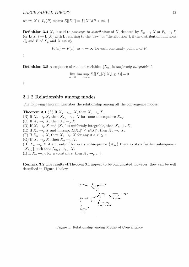
LARGE SAMPLE THEORY 43
where X ∈ Lr(P ) means E[|X|r] =∫ |X|rdP < ∞. †
Definition 3.4 Xn is said to converge in distribution of X, denoted by Xn →d X or Fn →d F(or L(Xn) → L(X) with L referring to the “law” or “distribution”), if the distribution functionsFn and F of Xn and X satisfy
Fn(x) → F (x) as n →∞ for each continuity point x of F.
†
Definition 3.5 A sequence of random variables Xn is uniformly integrable if
limλ→∞
lim supn→∞
E [|Xn|I(|Xn| ≥ λ)] = 0.
†
3.1.2 Relationship among modes
The following theorem describes the relationship among all the convergence modes.
Theorem 3.1 (A) If Xn →a.s. X, then Xn →p X.(B) If Xn →p X, then Xnk
→a.s. X for some subsequence Xnk.
(C) If Xn →r X, then Xn →p X.(D) If Xn →p X and |Xn|r is uniformly integrable, then Xn →r X.(E) If Xn →p X and lim supn E|Xn|r ≤ E|X|r, then Xn →r X.(F) If Xn →r X, then Xn →r′ X for any 0 < r′ ≤ r.(G) If Xn →p X, then Xn →d X.(H) Xn →p X if and only if for every subsequence Xnk
there exists a further subsequenceXnk,l such that Xnk,l →a.s. X.(I) If Xn →d c for a constant c, then Xn →p c. †
Remark 3.2 The results of Theorem 3.1 appear to be complicated; however, they can be welldescribed in Figure 1 below.
Figure 1: Relationship among Modes of Convergence
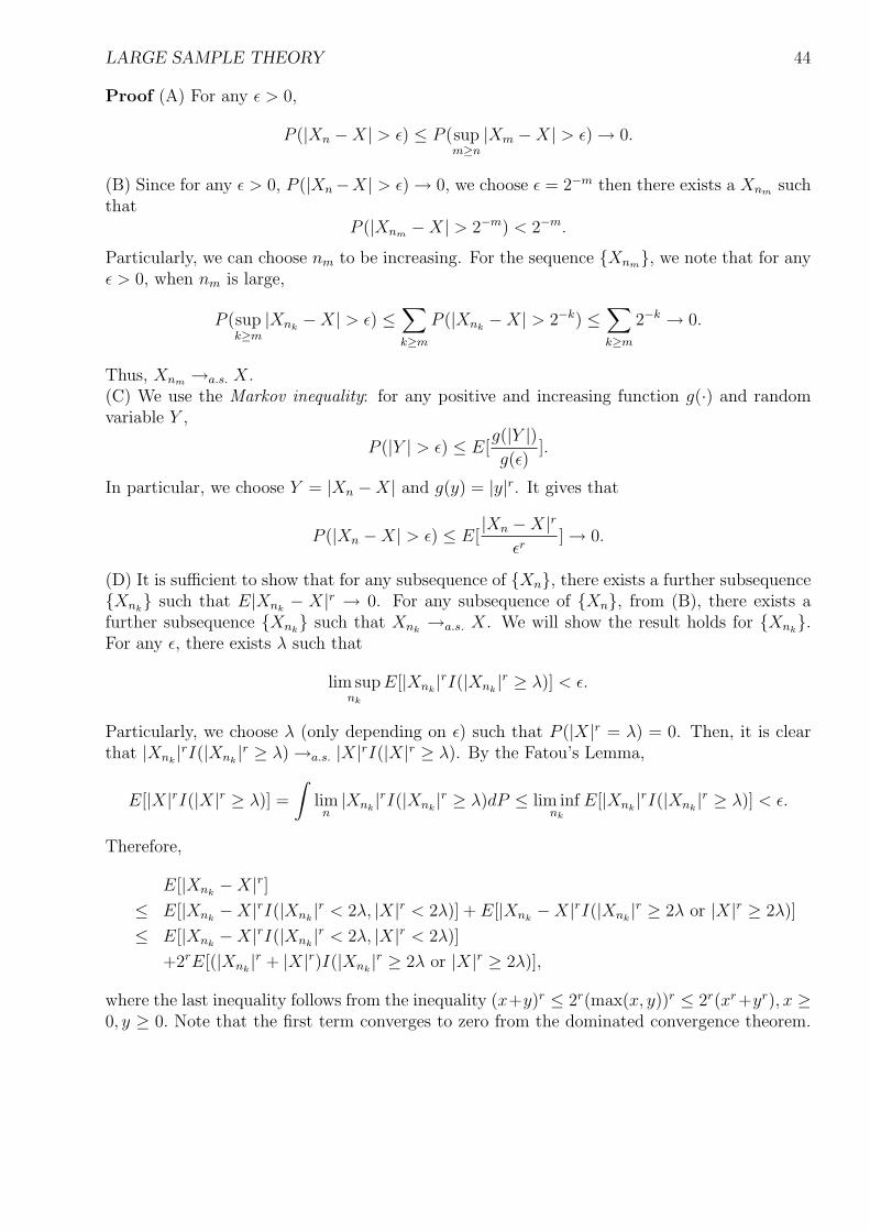
LARGE SAMPLE THEORY 44
Proof (A) For any ε > 0,
P (|Xn −X| > ε) ≤ P (supm≥n
|Xm −X| > ε) → 0.
(B) Since for any ε > 0, P (|Xn−X| > ε) → 0, we choose ε = 2−m then there exists a Xnm suchthat
P (|Xnm −X| > 2−m) < 2−m.
Particularly, we can choose nm to be increasing. For the sequence Xnm, we note that for anyε > 0, when nm is large,
P (supk≥m
|Xnk−X| > ε) ≤
∑
k≥m
P (|Xnk−X| > 2−k) ≤
∑
k≥m
2−k → 0.
Thus, Xnm →a.s. X.(C) We use the Markov inequality: for any positive and increasing function g(·) and randomvariable Y ,
P (|Y | > ε) ≤ E[g(|Y |)g(ε)
].
In particular, we choose Y = |Xn −X| and g(y) = |y|r. It gives that
P (|Xn −X| > ε) ≤ E[|Xn −X|r
εr] → 0.
(D) It is sufficient to show that for any subsequence of Xn, there exists a further subsequenceXnk
such that E|Xnk− X|r → 0. For any subsequence of Xn, from (B), there exists a
further subsequence Xnk such that Xnk
→a.s. X. We will show the result holds for Xnk.
For any ε, there exists λ such that
lim supnk
E[|Xnk|rI(|Xnk
|r ≥ λ)] < ε.
Particularly, we choose λ (only depending on ε) such that P (|X|r = λ) = 0. Then, it is clearthat |Xnk
|rI(|Xnk|r ≥ λ) →a.s. |X|rI(|X|r ≥ λ). By the Fatou’s Lemma,
E[|X|rI(|X|r ≥ λ)] =
∫lim
n|Xnk
|rI(|Xnk|r ≥ λ)dP ≤ lim inf
nk
E[|Xnk|rI(|Xnk
|r ≥ λ)] < ε.
Therefore,
E[|Xnk−X|r]
≤ E[|Xnk−X|rI(|Xnk
|r < 2λ, |X|r < 2λ)] + E[|Xnk−X|rI(|Xnk
|r ≥ 2λ or |X|r ≥ 2λ)]
≤ E[|Xnk−X|rI(|Xnk
|r < 2λ, |X|r < 2λ)]
+2rE[(|Xnk|r + |X|r)I(|Xnk
|r ≥ 2λ or |X|r ≥ 2λ)],
where the last inequality follows from the inequality (x+y)r ≤ 2r(max(x, y))r ≤ 2r(xr+yr), x ≥0, y ≥ 0. Note that the first term converges to zero from the dominated convergence theorem.
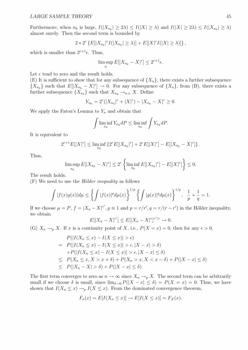
LARGE SAMPLE THEORY 45
Furthermore, when nk is large, I(|Xnk| ≥ 2λ) ≤ I(|X| ≥ λ) and I(|X| ≥ 2λ) ≤ I(|Xnk
| ≥ λ)almost surely. Then the second term is bounded by
2 ∗ 2r E[|Xnk|rI(|Xnk
| ≥ λ)] + E[|X|rI(|X| ≥ λ)] ,
which is smaller than 2r+1ε. Thus,
lim supn
E[|Xnk−X|r] ≤ 2r+1ε.
Let ε tend to zero and the result holds.(E) It is sufficient to show that for any subsequence of Xn, there exists a further subsequenceXnk
such that E[|Xnk− X|r] → 0. For any subsequence of Xn, from (B), there exists a
further subsequence Xnk such that Xnk
→a.s. X. Define
Ynk= 2r(|Xnk
|r + |X|r)− |Xnk−X|r ≥ 0.
We apply the Fatou’s Lemma to Yn and obtain that∫
lim infnk
YnkdP ≤ lim inf
nk
∫Ynk
dP.
It is equivalent to
2r+1E[|X|r] ≤ lim infnk
2rE[|Xnk|r] + 2rE[|X|r]− E[|Xnk
−X|r] .
Thus,
lim supnk
E[|Xnk−X|r] ≤ 2r
lim inf
nk
E[|Xnk|r]− E[|X|r]
≤ 0.
The result holds.(F) We need to use the Holder inequality as follows
∫|f(x)g(x)|dµ ≤
∫|f(x)|pdµ(x)
1/p ∫|g(x)|qdµ(x)
1/q
,1
p+
1
q= 1.
If we choose µ = P , f = |Xn−X|r′ , g ≡ 1 and p = r/r′, q = r/(r− r′) in the Holder inequality,we obtain
E[|Xn −X|r′ ] ≤ E[|Xn −X|r]r′/r → 0.
(G) Xn →p X. If x is a continuity point of X, i.e., P (X = x) = 0, then for any ε > 0,
P (|I(Xn ≤ x)− I(X ≤ x)| > ε)
= P (|I(Xn ≤ x)− I(X ≤ x)| > ε, |X − x| > δ)
+P (|I(Xn ≤ x)− I(X ≤ x)| > ε, |X − x| ≤ δ)
≤ P (Xn ≤ x,X > x + δ) + P (Xn > x,X < x− δ) + P (|X − x| ≤ δ)
≤ P (|Xn −X| > δ) + P (|X − x| ≤ δ).
The first term converges to zero as n →∞ since Xn →p X. The second term can be arbitrarilysmall if we choose δ is small, since limδ→0 P (|X − x| ≤ δ) = P (X = x) = 0. Thus, we haveshown that I(Xn ≤ x) →p I(X ≤ x). From the dominated convergence theorem,
Fn(x) = E[I(Xn ≤ x)] → E[I(X ≤ x)] = FX(x).

LARGE SAMPLE THEORY 46
Thus, Xn →d X.(H) One direction follows from (B). To prove the other direction, we use the contradiction.Suppose there exists ε > 0 such that P (|Xn −X| > ε) does not converge to zero. Then we canfind a subsequence Xn′ such hat P (|Xn′ − X| > ε) > δ for some δ > 0. However, by thecondition, we can choose a further subsequence Xn′′ such that Xn′′ →a.s. X then Xn′′ →p Xfrom A. This is a contradiction.(I) Let X ≡ c. It is clear from the following:
P (|Xn − c| > ε) ≤ 1− Fn(c + ε) + Fn(c− ε) → 1− FX(c + ε) + FX(c− ε) = 0.
†
Remark 3.3 Denote E[|X|r] as µr. Then as proving (F) in Theorem 3.1., we obtain µs−tr µr−s
t ≥µr−t
s where r ≥ s ≥ t ≥ 0. Thus, log µr is convex in r for r ≥ 0. Furthermore, the proof of (F )
says that µ1/rr is increasing in r.
Remark 3.4 For r ≥ 1, we denote E[|X|r]1/r as ‖X‖r (or ‖X‖Lr(P )). Clearly, ‖X‖r ≥ 0 andthe equality holds if and only if X = 0 a.s. For any constant λ, ‖λX‖r = |λ|‖X‖r. Furthermore,we note that
E[|X+Y |r] ≤ E[(|X|+|Y |)|X+Y |r−1] ≤ E[|X|r]1/rE[|X+Y |r]1−1/r+E[|Y |r]1/rE[|X+Y |r]1−1/r.
Then we obtain a triangular inequality (called the Minkowski’s inequality)
‖X + Y ‖r ≤ ‖X‖r + ‖Y ‖r.
Therefore, ‖ · ‖r in fact is a norm in the linear space X : ‖X‖r < ∞. Such a normed spaceis denoted as Lr(P ).
The following examples illustrate the results of Theorem 3.1.
Example 3.1 Suppose that Xn is degenerate at a point 1/n; i.e., P (Xn = 1/n) = 1. Then Xn
converges in distribution to zero. Indeed, Xn converges almost surely.
Example 3.2 X1, X2, ... are i.i.d with standard normal distribution. Then Xn →d X1 but Xn
does not converge in probability to X1.
Example 3.3 Let Z be a random variable with a uniform distribution in [0, 1]. Let Xn =I(m2−k ≤ Z < (m + 1)2−k) when n = 2k + m where 0 ≤ m < 2k. Then Xn converges inprobability to zero but not almost surely. This example is already given in the second chapter.
Example 3.4 Let Z be Uniform(0, 1) and let Xn = 2nI(0 ≤ Z < 1/n). Then E[|Xn|r]] →∞but Xn converges to zero almost surely.
The next theorem describes the necessary and sufficient conditions of convergence in mo-ments from convergence in probability.
Theorem 3.2 (Vitali’s theorem) Suppose that Xn ∈ Lr(P ), i.e., ‖Xn‖r < ∞, where 0 <r < ∞ and Xn →p X. Then the following are equivalent:(A) |Xn|r are uniformly integrable.
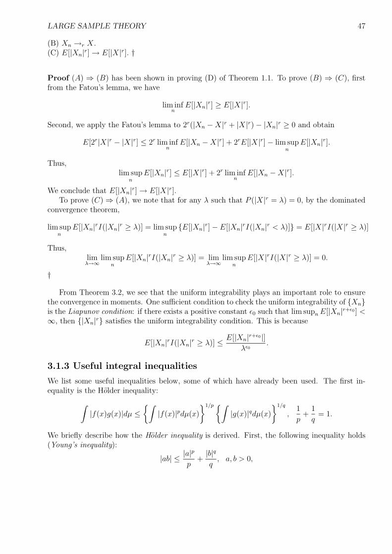
LARGE SAMPLE THEORY 47
(B) Xn →r X.(C) E[|Xn|r] → E[|X|r]. †
Proof (A) ⇒ (B) has been shown in proving (D) of Theorem 1.1. To prove (B) ⇒ (C), firstfrom the Fatou’s lemma, we have
lim infn
E[|Xn|r] ≥ E[|X|r].
Second, we apply the Fatou’s lemma to 2r(|Xn −X|r + |X|r)− |Xn|r ≥ 0 and obtain
E[2r|X|r − |X|r] ≤ 2r lim infn
E[|Xn −X|r] + 2rE[|X|r]− lim supn
E[|Xn|r].
Thus,lim sup
nE[|Xn|r] ≤ E[|X|r] + 2r lim inf
nE[|Xn −X|r].
We conclude that E[|Xn|r] → E[|X|r].To prove (C) ⇒ (A), we note that for any λ such that P (|X|r = λ) = 0, by the dominated
convergence theorem,
lim supn
E[|Xn|rI(|Xn|r ≥ λ)] = lim supn
E[|Xn|r]− E[|Xn|rI(|Xn|r < λ)] = E[|X|rI(|X|r ≥ λ)]
Thus,lim
λ→∞lim sup
nE[|Xn|rI(|Xn|r ≥ λ)] = lim
λ→∞lim sup
nE[|X|rI(|X|r ≥ λ)] = 0.
†
From Theorem 3.2, we see that the uniform integrability plays an important role to ensurethe convergence in moments. One sufficient condition to check the uniform integrability of Xnis the Liapunov condition: if there exists a positive constant ε0 such that lim supn E[|Xn|r+ε0 ] <∞, then |Xn|r satisfies the uniform integrability condition. This is because
E[|Xn|rI(|Xn|r ≥ λ)] ≤ E[|Xn|r+ε0|]λε0
.
3.1.3 Useful integral inequalities
We list some useful inequalities below, some of which have already been used. The first in-equality is the Holder inequality:
∫|f(x)g(x)|dµ ≤
∫|f(x)|pdµ(x)
1/p ∫|g(x)|qdµ(x)
1/q
,1
p+
1
q= 1.
We briefly describe how the Holder inequality is derived. First, the following inequality holds(Young’s inequality):
|ab| ≤ |a|pp
+|b|qq
, a, b > 0,
LARGE SAMPLE THEORY 48
where the equality holds if and only if a = b. This inequality is clear from its geometric meaning.In this inequality, we choose a = f(x)/
∫ |f(x)|pdµ(x)1/p and b = g(x)/∫ |g(x)|qdµ(x)1/q
and integrate over x on both side. It gives the Holder inequality and the equality holds if andonly if f(x) is proportional to g(x) almost surely. When p = q = 2, the inequality becomes
∫|f(x)g(x)|dµ(x) ≤
∫f(x)2dµ(x)
1/2 ∫g(x)2dµ(x)
1/2
,
which is the Cauchy-Schwartz inequality. One implication is that for non-trivial X and Y ,(E[|XY |])2 ≤ E[|X|2]E[|Y |2] and that the equality holds if and only if |X| = c0|Y | almostsurely for some constant c0.
A second important inequality is the Markov’s inequality, which was used in proving (C) ofTheorem 3.1:
P (|X| ≥ ε) ≤ E[g(|X|)]g(ε)
,
where g ≥ 0 is a increasing function in [0,∞). We can choose different g to obtain many similarinequalities. The proof of the Markov inequality is direct from the following:
P (|Y | > ε) = E[I(|Y | > ε)] ≤ E[g(|Y |)g(ε)
I(|Y | > ε)] ≤ E[g(|Y |)g(ε)
].
If we choose g(x) = x2 and X as X − E[X] in the Markov inequality, we obtain
P (|X − E[X]| ≥ ε) ≤ V ar(X)
ε2.
This inequality is the Chebychev’s inequality and gives an upper bound for controlling the tailprobability of X using its variance.
In summary, we have introduced different modes of convergence for random variables andobtained the relationship among these modes. The same definitions and relationship can begeneralized to random vectors. One additional remark is that since convergence almost surelyor in probability are special definitions of convergence almost everywhere or in measure as givenin the second chapter, all the theorems in Section 2.3.3 including the monotone convergencetheorem, the Fatou’s lemma and the dominated convergence theorem should apply. Conver-gence in distribution is the only one specific to probability measure. In fact, this model will bethe main interest of the subsequent sections.
3.2 Convergence in Distribution
Among all the convergence modes of Xn, convergence in distribution is the weakest conver-gence. However, this convergence plays an important and sufficient role in statistical inference,especially when large sample behavior of random variables is of interest. We focus on suchparticular convergence in this section.
3.2.1 Portmanteau theorem
The following theorem gives all equivalent conditions to the convergence in distribution for asequence of random variables Xn.
LARGE SAMPLE THEORY 49
Theorem 3.3 (Portmanteau Theorem) The following conditions are equivalent.(a) Xn converges in distribution to X.(b) For any bounded continuous function g(·), E[g(Xn)] → E[g(X)].(c) For any open set G in R, lim infn P (Xn ∈ G) ≥ P (X ∈ G).(d) For any closed set F in R, lim supn P (Xn ∈ F ) ≤ P (X ∈ F ).(e) For any Borel set O in R with P (X ∈ ∂O) = 0 where ∂O is the boundary of O, P (Xn ∈O) → P (X ∈ O). †
Proof (a) ⇒ (b). Without loss of generality, we assume |g(x)| ≤ 1. We choose [−M,M ] suchthat P (|X| = M) = 0. Since g is continuous in [−M, M ], g is uniformly continuous in [−M,M ].Thus for any ε, we can partition [−M,M ] into finite intervals I1 ∪ ... ∪ Im such that withineach interval Ik, maxIk
g(x)−minIkg(x) ≤ ε and X has no mass at all the endpoints of Ik (this
is feasible since X has at most countable points with point masses). Therefore, if choose anypoint xk ∈ Ik, k = 1, ..., m,
|E[g(Xn)]− E[g(X)]|≤ E[|g(Xn)|I(|Xn| > M)] + E[|g(X)|I(|X| > M)]
+|E[g(Xn)I(|Xn| ≤ M)]−m∑
k=1
g(xk)P (Xn ∈ Ik)|
+|m∑
k=1
g(xk)P (Xn ∈ Ik)−m∑
k=1
g(xk)P (X ∈ Ik)|
+|E[g(X)I(|X| ≤ M)]−m∑
k=1
g(xk)P (X ∈ Ik)|
≤ P (|Xn| > M) + P (|X| > M) + 2ε +m∑
k=1
|P (Xn ∈ Ik)− P (X ∈ Ik)|.
Thus, lim supn |E[g(Xn)]−E[g(X)]| ≤ 2P (|X| > M) + 2ε. Let M →∞ and ε → 0. We obtain(b).(b) ⇒ (c). For any open set G, we define a function
g(x) = 1− ε
ε + d(x,Gc),
where d(x,Gc) is the minimal distance between x and Gc, defined as infy∈Gc |x− y|. Since forany y ∈ Gc,
d(x1, Gc)− |x2 − y| ≤ |x1 − y| − |x2 − y| ≤ |x1 − x2|,
we have d(x1, Gc)− d(x2, G
c) ≤ |x1 − x2|. Then,
|g(x1)− g(x2)| ≤ ε−1|d(x1, Gc)− d(x2, G
c)| ≤ ε−1|x1 − x2|.
g(x) is continuous and bounded. From (a), E[g(Xn)] → E[g(X)]. Note g(x) = 0 if x /∈ G and|g(x)| ≤ 1. Thus,
lim infn
P (Xn ∈ G) ≥ lim infn
E[g(Xn)] → E[g(X)].
LARGE SAMPLE THEORY 50
Let ε → 0 and we obtain E[g(X)] converges to E[I(X ∈ G)] = P (X ∈ G).(c) ⇒ (d). This is clear by taking complement of F .(d) ⇒ (e). For any O with P (X ∈ ∂O) = 0, we have
lim supn
P (Xn ∈ O) ≤ lim supn
P (Xn ∈ O) ≤ P (X ∈ O) = P (X ∈ O),
andlim inf
nP (Xn ∈ O) ≥ lim inf
nP (Xn ∈ Oo) ≥ P (X ∈ Oo) = P (X ∈ O).
Here, O and Oo are the closure and interior of O respectively.(e) ⇒ (a). It is clear by choosing O = (−∞, x] with P (X ∈ ∂O) = P (X = x) = 0. †
The conditions in Theorem 3.3 are necessary, as seen in the following examples.
Example 3.5 Let g(x) = x, a continuous but unbounded function. Let Xn be a randomvariable taking value n with probability 1/n and value 0 with probability (1 − 1/n). ThenXn →d 0. However, E[g(X)] = 1 9 0. This shows that the boundness of g in condition (b) isnecessary.
Example 3.6 The continuity at boundary in (e) is also necessary: let Xn be degenerate at 1/nand consider O = x : x > 0. Then P (Xn ∈ O) = 1 but Xn →d 0.
3.2.2 Continuity theorem
Another way of verifying convergence in distribution of Xn is via the convergence of the char-acteristic functions of Xn, as given in the following theorem. This result is very useful in manyapplications.
Theorem 3.4 (Continuity Theorem) Let φn and φ denote the characteristic functions ofXn and X respectively. Then Xn →d X is equivalent to φn(t) → φ(t) for each t. †
Proof To prove ⇒ direction, from (b) in Theorem 3.1,
φn(t) = E[eitXn ] → E[eitX ] = φ(t).
We thus need to prove ⇐ direction. This proof consists of the following steps.Step 1. We show that for any ε, there exists a M such that supn P (|Xn| > M) < ε. Thisproperty is called asymptotic tightness of Xn. To see that, we note that
1
δ
∫ δ
−δ
(1− φn(t))dt = E[1
δ
∫ δ
−δ
(1− eitXn)dt]
= E[2(1− sin δXn
δXn
)]
≥ E[2(1− 1
|δXn|)I(|Xn| > 2
δ)]
≥ P (|Xn| > 2
δ).
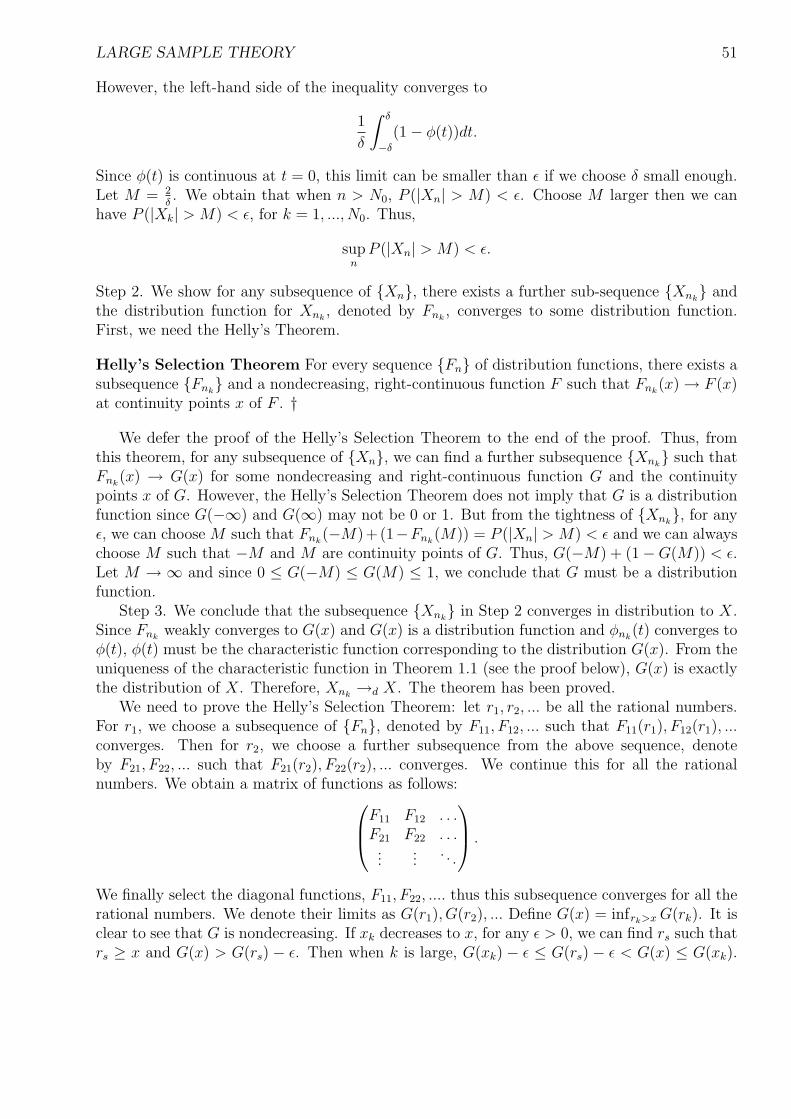
LARGE SAMPLE THEORY 51
However, the left-hand side of the inequality converges to
1
δ
∫ δ
−δ
(1− φ(t))dt.
Since φ(t) is continuous at t = 0, this limit can be smaller than ε if we choose δ small enough.Let M = 2
δ. We obtain that when n > N0, P (|Xn| > M) < ε. Choose M larger then we can
have P (|Xk| > M) < ε, for k = 1, ..., N0. Thus,
supn
P (|Xn| > M) < ε.
Step 2. We show for any subsequence of Xn, there exists a further sub-sequence Xnk and
the distribution function for Xnk, denoted by Fnk
, converges to some distribution function.First, we need the Helly’s Theorem.
Helly’s Selection Theorem For every sequence Fn of distribution functions, there exists asubsequence Fnk
and a nondecreasing, right-continuous function F such that Fnk(x) → F (x)
at continuity points x of F . †
We defer the proof of the Helly’s Selection Theorem to the end of the proof. Thus, fromthis theorem, for any subsequence of Xn, we can find a further subsequence Xnk
such thatFnk
(x) → G(x) for some nondecreasing and right-continuous function G and the continuitypoints x of G. However, the Helly’s Selection Theorem does not imply that G is a distributionfunction since G(−∞) and G(∞) may not be 0 or 1. But from the tightness of Xnk
, for anyε, we can choose M such that Fnk
(−M)+(1−Fnk(M)) = P (|Xn| > M) < ε and we can always
choose M such that −M and M are continuity points of G. Thus, G(−M) + (1−G(M)) < ε.Let M → ∞ and since 0 ≤ G(−M) ≤ G(M) ≤ 1, we conclude that G must be a distributionfunction.
Step 3. We conclude that the subsequence Xnk in Step 2 converges in distribution to X.
Since Fnkweakly converges to G(x) and G(x) is a distribution function and φnk
(t) converges toφ(t), φ(t) must be the characteristic function corresponding to the distribution G(x). From theuniqueness of the characteristic function in Theorem 1.1 (see the proof below), G(x) is exactlythe distribution of X. Therefore, Xnk
→d X. The theorem has been proved.We need to prove the Helly’s Selection Theorem: let r1, r2, ... be all the rational numbers.
For r1, we choose a subsequence of Fn, denoted by F11, F12, ... such that F11(r1), F12(r1), ...converges. Then for r2, we choose a further subsequence from the above sequence, denoteby F21, F22, ... such that F21(r2), F22(r2), ... converges. We continue this for all the rationalnumbers. We obtain a matrix of functions as follows:
F11 F12 . . .F21 F22 . . ....
.... . .
.
We finally select the diagonal functions, F11, F22, .... thus this subsequence converges for all therational numbers. We denote their limits as G(r1), G(r2), ... Define G(x) = infrk>x G(rk). It isclear to see that G is nondecreasing. If xk decreases to x, for any ε > 0, we can find rs such thatrs ≥ x and G(x) > G(rs) − ε. Then when k is large, G(xk) − ε ≤ G(rs) − ε < G(x) ≤ G(xk).
LARGE SAMPLE THEORY 52
That is, limk G(xk) = G(x). Thus, G is right-continuous. If x is a continuity point of G, forany ε, we can find two sequence of rational number rk and rk′ such that rk decreases to xand rk′ increases to x. Then after taking limits for the inequality Fll(rk′) ≤ Fll(x) ≤ Fll(rk), wehave
G(rk′) ≤ lim infl
Fll(x) ≤ lim supl
Fll(x) ≤ G(rk).
Let k →∞ then we obtain liml Fll(x) = G(x).It remains to prove Theorem 1.1, whose proof is deferred here: after substituting φ(t) in to
the integration, we obtain
1
2π
∫ T
−T
e−ita − e−itb
itφ(t)dt =
1
2π
∫ T
−T
∫ ∞
−∞
e−ita − e−itb
iteitxdF (x)dt
=1
2π
∫ ∞
−∞
∫ T
−T
eit(x−a) − eit(x−b)
itdtdF (x).
The interchange of the integrations follows from the Fubini’s theorem. The last part is equal
∫ ∞
−∞
sgn(x− a)
π
∫ T |x−a|
0
sin t
tdt− sgn(x− b)
π
∫ T |x−b|
0
sin t
tdt
dF (x).
The integrand is bounded by 2π
∫∞0
sin tt
dt and as T → ∞, it converges to 0, if x < a or x > b;1/2, if x = a or x = b; 1, if x ∈ (a, b). Therefore, by the dominated convergence theorem, theintegral converges to
F (b−)− F (a) +1
2F (b)− F (b−)+
1
2F (a)− F (a−) .
Since F is continuous at b and a, the limit is the same as F (b)− F (a). Furthermore, supposethat F has a density function f . Then
F (x)− F (0) =1
2π
∫ ∞
−∞
1− e−itx
itφ(t)dt.
Since | ∂∂x
1−e−itx
itφ(t)| ≤ φ(t), according to the interchange between derivative and integration,
we obtain
f(x) =1
2π
∫ ∞
−∞e−itxφ(t)dt.
†
The above theorem indicates that to prove the weak convergence of a sequence of randomvariables, it is sufficient to check the convergence of their characteristic functions. For example,if X1, ..., Xn are i.i.d Bernoulli(p), then the characteristic function of Xn = (X1 + ... + Xn)/n isgiven by (1−p+peit/n)n converges to a function φ(t) = eitp, which is the characteristic functionfor a degenerate random variable X ≡ p. Thus Xn converges in distribution to p. Then fromTheorem 3.1, Xn converges in probability to p.
Theorem 3.4 also has a multivariate version when Xn and X are k-dimensional randomvectors: Xn →d X if and only if E[expit ′Xn] → E [expit ′X ], where t is any k-dimensional
LARGE SAMPLE THEORY 53
constant. Since the latter is equivalent to the weak convergence of t′Xn to t′X, we concludethat the weak convergence of Xn to X is equivalent to the weak convergence of t′Xn to t′Xfor any t. That is, to study the weak convergence of random vectors, we can reduce to studythe weak convergence of one-dimensional linear combination of the random vectors. This is thewell-known Cramer-Wold’s device:
Theorem 3.5 (The Cramer-Wold device) Random vector Xn in Rk satisfy Xn →d X ifand only t′Xn →d t′X in R for all t ∈ Rk. †
3.2.3 Properties of convergence in distribution
Some additional results from convergence in distribution are the following theorems.
Theorem 3.6 (Continuous mapping theorem) Suppose Xn →a.s. X, or Xn →p X, orXn →d X. Then for any continuous function g(·), g(Xn) converges to g(X) almost surely, orin probability, or in distribution. †
Proof If Xn →a.s. X, then clearly, g(Xn) →a.s g(X). If Xn →p X, then for any subsequence,there exists a further subsequence Xnk
→a.s. X. Thus, g(Xnk) →a.s. g(X). Then g(Xn) →p
g(X) from (H) in Theorem 3.1. To prove that g(Xn) →d g(X) when Xn →d X, we apply (b)of Theorem 3.3. †
Remark 3.5 Theorem 3.6 concludes that g(Xn) →d g(X) if Xn →d X and g is continuous. Infact, this result still holds if P (X ∈ C(g)) = 1 where C(g) contains all the continuity pointsof g. That is, if g’s discontinuity points take zero probability of X, the continuous mappingtheorem holds.
Theorem 3.7 (Slutsky theorem) Suppose Xn →d X, Yn →p y and Zn →p z for someconstant y and z. Then ZnXn + Tn →d zX + y. †
Proof We first show that Xn + Yn →d X + y. For any ε > 0,
P (Xn + Yn ≤ x) ≤ P (Xn + Yn ≤ x, |Yn − y| ≤ ε) + P (|Yn − y| > ε)
≤ P (Xn ≤ x− y + ε) + P (|Yn − y| > ε).
Thus,lim sup
nFXn+Yn(x) ≤ lim sup
nFXn(x− y + ε) ≤ FX(x− y + ε).
On the other hand,
P (Xn + Yn > x) = P (Xn + Yn > x, |Yn − y| ≤ ε) + P (|Yn − y| > ε)
≤ P (Xn > x− y − ε) + P (|Yn − y| > ε).
LARGE SAMPLE THEORY 54
Thus,
lim supn
(1− FXn+Yn(x)) ≤ lim supn
P (Xn > x− y − ε) ≤ lim supn
P (Xn ≥ x− y − 2ε)
≤ (1− FX(x− y − 2ε)).
We obtain
FX(x− y − 2ε) ≤ lim infn
FXn+Yn(x) ≤ lim supn
FXn+Yn(x) ≤ FX(x + y + ε).
Let ε → 0 then it holds
FX+y(x−) ≤ lim infn
FXn+Yn(x) ≤ lim supn
FXn+Yn(x) ≤ FX+y(x).
Thus, Xn + Yn →d X + y.On the other hand, we have
P (|(Zn − z)Xn| > ε) ≤ P (|Zn − z| > ε2) + P (|Zn − z| ≤ ε2, |Xn| > 1
ε).
Thus,
lim supn
P (|(Zn− z)Xn| > ε) ≤ lim supn
P (|Zn− z| > ε2)+ lim supn
P (|Xn| ≥ 1
2ε) → P (|X| ≥ 1
2ε).
Since ε is arbitrary, we conclude that (Zn− z)Xn →p 0. Clearly zXn →d zX. Hence, ZnXn →d
zX from the proof in the first half. Again, using the first half’s proof, we obtain ZnXn +Yn →d
zX + y. †
Remark 3.6 In the proof of Theorem 3.7, if we replace Xn + Yn by aXn + bYn, we can showthat aXn + bYn →d aX + by by considering different cases of either a or b or both are non-zeros.Then from Theorem 3.5, (Xn, Yn) →d (X, y) in R2. By the continuity theorem, we obtainXn + Yn →d X + y and XnYn →d Xy. This immediately gives Theorem 3.7.
Both Theorems 3.6 and 3.7 are useful in deriving the convergence of some transformedrandom variables, as shown in the following examples.
Example 3.7 Suppose Xn →d N(0, 1). Then by continuous mapping theorem, X2n →d χ2
1.
Example 3.8 This example shows that g can be discontinuous in Theorem 3.6. Let Xn →d Xwith X ∼ N(0, 1) and g(x) = 1/x. Although g(x) is discontinuous at origin, we can still showthat 1/Xn →d 1/X, the reciprocal of the normal distribution. This is because P (X = 0) = 0.However, in Example 3.6 where g(x) = I(x > 0), it shows that Theorem 3.6 may not be trueif P (X ∈ C(g)) < 1.
Example 3.9 The condition Yn →p y, where y is a constant, is necessary. For example, letXn = X ∼ Uniform(0, 1). Let Yn = −X so Yn →d −X, where X is an independent randomvariable with the same distribution as X. However Xn+Yn = 0 does not converge in distributionto the non-zero random variable X − X.
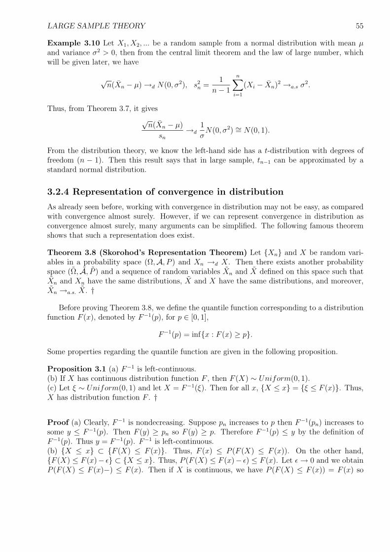
LARGE SAMPLE THEORY 55
Example 3.10 Let X1, X2, ... be a random sample from a normal distribution with mean µand variance σ2 > 0, then from the central limit theorem and the law of large number, whichwill be given later, we have
√n(Xn − µ) →d N(0, σ2), s2
n =1
n− 1
n∑i=1
(Xi − Xn)2 →a.s σ2.
Thus, from Theorem 3.7, it gives
√n(Xn − µ)
sn
→d1
σN(0, σ2) ∼= N(0, 1).
From the distribution theory, we know the left-hand side has a t-distribution with degrees offreedom (n − 1). Then this result says that in large sample, tn−1 can be approximated by astandard normal distribution.
3.2.4 Representation of convergence in distribution
As already seen before, working with convergence in distribution may not be easy, as comparedwith convergence almost surely. However, if we can represent convergence in distribution asconvergence almost surely, many arguments can be simplified. The following famous theoremshows that such a representation does exist.
Theorem 3.8 (Skorohod’s Representation Theorem) Let Xn and X be random vari-ables in a probability space (Ω,A, P ) and Xn →d X. Then there exists another probabilityspace (Ω, A, P ) and a sequence of random variables Xn and X defined on this space such thatXn and Xn have the same distributions, X and X have the same distributions, and moreover,Xn →a.s. X. †
Before proving Theorem 3.8, we define the quantile function corresponding to a distributionfunction F (x), denoted by F−1(p), for p ∈ [0, 1],
F−1(p) = infx : F (x) ≥ p.
Some properties regarding the quantile function are given in the following proposition.
Proposition 3.1 (a) F−1 is left-continuous.(b) If X has continuous distribution function F , then F (X) ∼ Uniform(0, 1).(c) Let ξ ∼ Uniform(0, 1) and let X = F−1(ξ). Then for all x, X ≤ x = ξ ≤ F (x). Thus,X has distribution function F . †
Proof (a) Clearly, F−1 is nondecreasing. Suppose pn increases to p then F−1(pn) increases tosome y ≤ F−1(p). Then F (y) ≥ pn so F (y) ≥ p. Therefore F−1(p) ≤ y by the definition ofF−1(p). Thus y = F−1(p). F−1 is left-continuous.(b) X ≤ x ⊂ F (X) ≤ F (x). Thus, F (x) ≤ P (F (X) ≤ F (x)). On the other hand,F (X) ≤ F (x)− ε ⊂ X ≤ x. Thus, P (F (X) ≤ F (x)− ε) ≤ F (x). Let ε → 0 and we obtainP (F (X) ≤ F (x)−) ≤ F (x). Then if X is continuous, we have P (F (X) ≤ F (x)) = F (x) so
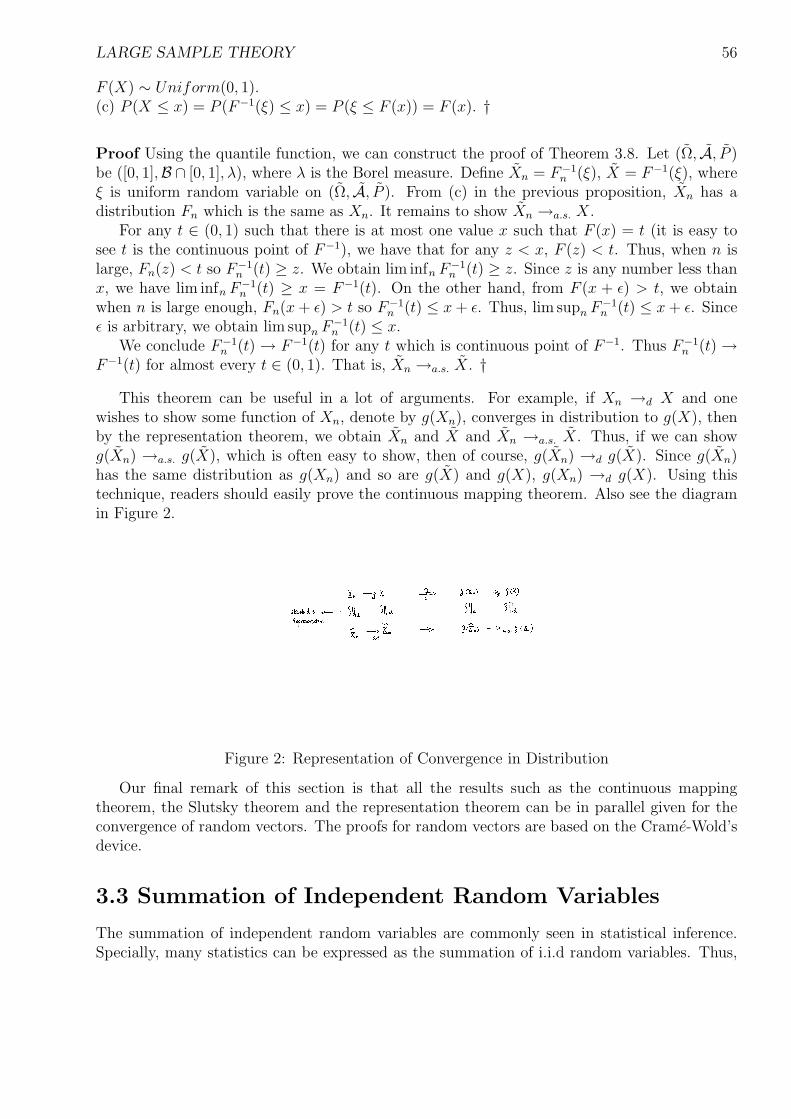
LARGE SAMPLE THEORY 56
F (X) ∼ Uniform(0, 1).(c) P (X ≤ x) = P (F−1(ξ) ≤ x) = P (ξ ≤ F (x)) = F (x). †
Proof Using the quantile function, we can construct the proof of Theorem 3.8. Let (Ω, A, P )be ([0, 1],B ∩ [0, 1], λ), where λ is the Borel measure. Define Xn = F−1
n (ξ), X = F−1(ξ), whereξ is uniform random variable on (Ω, A, P ). From (c) in the previous proposition, Xn has adistribution Fn which is the same as Xn. It remains to show Xn →a.s. X.
For any t ∈ (0, 1) such that there is at most one value x such that F (x) = t (it is easy tosee t is the continuous point of F−1), we have that for any z < x, F (z) < t. Thus, when n islarge, Fn(z) < t so F−1
n (t) ≥ z. We obtain lim infn F−1n (t) ≥ z. Since z is any number less than
x, we have lim infn F−1n (t) ≥ x = F−1(t). On the other hand, from F (x + ε) > t, we obtain
when n is large enough, Fn(x + ε) > t so F−1n (t) ≤ x + ε. Thus, lim supn F−1
n (t) ≤ x + ε. Sinceε is arbitrary, we obtain lim supn F−1
n (t) ≤ x.We conclude F−1
n (t) → F−1(t) for any t which is continuous point of F−1. Thus F−1n (t) →
F−1(t) for almost every t ∈ (0, 1). That is, Xn →a.s. X. †This theorem can be useful in a lot of arguments. For example, if Xn →d X and one
wishes to show some function of Xn, denote by g(Xn), converges in distribution to g(X), thenby the representation theorem, we obtain Xn and X and Xn →a.s. X. Thus, if we can showg(Xn) →a.s. g(X), which is often easy to show, then of course, g(Xn) →d g(X). Since g(Xn)has the same distribution as g(Xn) and so are g(X) and g(X), g(Xn) →d g(X). Using thistechnique, readers should easily prove the continuous mapping theorem. Also see the diagramin Figure 2.
Figure 2: Representation of Convergence in Distribution
Our final remark of this section is that all the results such as the continuous mappingtheorem, the Slutsky theorem and the representation theorem can be in parallel given for theconvergence of random vectors. The proofs for random vectors are based on the Crame-Wold’sdevice.
3.3 Summation of Independent Random Variables
The summation of independent random variables are commonly seen in statistical inference.Specially, many statistics can be expressed as the summation of i.i.d random variables. Thus,
LARGE SAMPLE THEORY 57
this section gives some classical large sample results for this type of statistics, which includethe weak/strong law of large numbers, the central limit theorem, and the Delta method etc.
3.3.1 Preliminary lemma
Proposition 3.2 (Borel-Cantelli Lemma) For any events An,
∞∑i=1
P (An) < ∞
implies P (An, i.o.) = P (An occurs infinitely often) = 0; or equivalently, P (∩∞n=1 ∪m≥n Am) =0. †
ProofP (An, i.o) ≤ P (∪m≥nAm) ≤
∑m≥n
P (Am) → 0, as n →∞.
†
As a result of the proposition, if for a sequence of random variables, Zn, and for any ε > 0,∑n P (|Zn| > ε) < ∞. Then with probability one, |Zn| > ε only occurs finite times. That is,
Zn →a.s. 0.
Proposition 3.3 (Second Borel-Cantelli Lemma) For a sequence of independent eventsA1, A2, ...,
∑∞n=1 P (An) = ∞ implies P (An, i.o.) = 1. †
Proof Consider the complement of An, i.o. Note
P (∪∞n=1 ∩m≥n Acm) = lim
nP (∩m≥nA
cm) = lim
n
∏m≥n
(1− P (Am)) ≤ lim supn
exp−∑m≥n
P (Am) = 0.
†
Proposition 3.4 X,X1, ..., Xn are i.i.d with finite mean. Define Yn = XnI(|Xn| ≤ n). Then∑∞n=1 P (Xn 6= Yn) < ∞. †
Proof Since E[|X|] < ∞,
∞∑n=1
P (Xn 6= Yn) ≤∞∑
n=1
P (|X| ≥ n) =∞∑
n=1
nP (n ≤ |X| < (n + 1)) ≤∞∑
n=1
E[|X|] < ∞.
From the Borel-Cantelli Lemma, P (Xn 6= Yn, i.o) = 0. That is, for almost every ω ∈ Ω, whenn is large enough, Xn(ω) = Yn(ω). †
LARGE SAMPLE THEORY 58
3.3.2 Law of large numbers
We start to prove the weak and strong law of large numbers.
Theorem 3.9 (Weak Law of Large Number) If X, X1, ..., Xn are i.i.d with mean µ (soE[|X|] < ∞ and µ = E[X]), then Xn →p µ. †
Proof Define Yn = XnI(−n ≤ Xn ≤ n). Let µn =∑n
k=1 E[Yk]/n. Then by the Chebyshev’sinequality,
P (|Yn − µn| ≥ ε) ≤ V ar(Yn)
ε2≤
∑nk=1 V ar(XkI(|Xk| ≤ k))
n2ε2.
Since
V ar(XkI(|Xk| ≤ k)) ≤ E[X2kI(|Xk| ≤ k)]
= E[X2kI(|Xk| ≤ k, |Xk| ≥
√kε2)] + E[X2
kI(|Xk| ≤ k, |X| ≤√
kε2)]
≤ kE[|Xk|I(|Xk| ≥√
kε2)] + kε4,
P (|Yn − µn| ≥ ε) ≤∑n
k=1 E[|X|I(|X| ≥√
kε2)]
nε2+ ε2n(n + 1)
2n2.
Thus, lim supn P (|Yn − µn| ≥ ε) ≤ ε2. We conclude that Yn − µn →p 0. On the other hand,µn → µ. We obtain Yn →p µ. This implies that for any subsequence, there is a furthersubsequence Ynk →a.s. µ. Since Xn is eventually the same as Yn for almost every ω fromProposition 3.4, we conclude Xnk →a.s. µ. This implies Xn →p µ. †
Theorem 3.10 (Strong Law of Large Number) If X1, ..., Xn are i.i.d with mean µ thenXn →a.s. µ. †
Proof Without loss of generality, we assume Xn ≥ 0 since if this is true, the result also holdsfor any Xn by Xn = X+
n −X−n .
Similar to Theorem 3.9, it is sufficient to show Yn →a.s. µ, where Yn = XnI(Xn ≤ n). NoteE[Yn] = E[X1I(X1 ≤ n)] → µ so
n∑
k=1
E[Yk]/n → µ.
Thus, if we denote Sn =∑n
k=1(Yk−E[Yk]) and we can show Sn/n →a.s. 0, then the result holds.Note
V ar(Sn) =n∑
k=1
V ar(Yk) ≤n∑
k=1
E[Y 2k ] ≤ nE[X2
1I(X1 ≤ n)].
Then by the Chebyshev’s inequality,
P (| Sn
n| > ε) ≤ 1
n2ε2V ar(Sn) ≤ E[X2
1I(X1 ≤ n)]
nε2.
LARGE SAMPLE THEORY 59
For any α > 1, let un = [αn]. Then
∞∑n=1
P (| Sun
un
| > ε) ≤∞∑
n=1
1
unε2E[X2
1I(X1 ≤ un)] ≤ 1
ε2E[X2
1
∑un≥X1
1
un
].
Since for any x > 0,∑
un≥xµn−1 < 2∑
n≥log x/ log α α−n ≤ Kx−1 for some constant K, wehave ∞∑
n=1
P (| Sun
un
| > ε) ≤ K
ε2E[X1] < ∞,
From the Borel-Cantelli Lemma in Proposition 3.2, Sun/un →a.s. 0.For any k, we can find un < k ≤ un+1. Thus, since X1, X2, ... ≥ 0,
Sun
un
un
un+1
≤ Sk
k≤ Sun+1
un+1
un+1
un
.
After taking limits in the above, we have
µ/α ≤ lim infk
Sk
k≤ lim sup
k
Sk
k≤ µα.
Since α is arbitrary number larger than 1, let α → 1 and we obtain limk Sk/k = µ. The proofis completed. †
3.3.3 Central limit theorem
We now consider the central limit theorem. All the proofs can be based on the convergence ofthe corresponding characteristic function. The following lemma describes the approximation ofa characteristic function.
Proposition 3.5 Suppose E[|X|m] < ∞ for some integer m ≥ 0. Then
|φX(t)−m∑
k=0
(it)k
k!E[Xk]|/|t|m → 0, as t → 0.
†
Proof We note the following expansion for eitx,
eitx =m∑
k=1
(itx)k
k!+
(itx)m
m![eitθx − 1],
where θ ∈ [0, 1]. Thus,
|φX(t)−m∑
k=0
(it)k
k!E[Xk]|/|t|m ≤ E[|X|m|eitθX − 1|]/m! → 0,
LARGE SAMPLE THEORY 60
as t → 0. †
Theorem 3.11 (Central Limit Theorem) If X1, ..., Xn are i.i.d with mean µ and varianceσ2 then
√n(Xn − µ) →d N(0, σ2). †
Proof Denote Yn =√
n(Xn − µ). We consider the characteristic function of Yn.
φYn(t) =φX1−µ(t/
√n)
n.
Using Proposition 3.5, we have φX1−µ(t/√
n) = 1− σ2t2/2n + o(1/n). Thus,
φYn(t) → exp−σ2t2
2.
The result holds. †
Theorem 3.12 (Multivariate Central Limit Theorem) If X1, ..., Xn are i.i.d randomvectors in Rk with mean µ and covariance Σ = E[(X−µ)(X−µ)′], then
√n(Xn−µ) →d N(0, Σ).
†
Proof Similar to Theorem 3.11, but this time, we consider a multivariate characteristic functionE[expi√nt′(Xn − µ)]. Note the result of Proposition 3.5 holds for this multivariate case. †
Theorem 3.13 (Liapunov Central Limit Theorem) Let Xn1, ..., Xnn be independent ran-dom variables with µni = E[Xni] and σ2
ni = V ar(Xni). Let µn =∑n
i=1 µni, σ2n =
∑ni=1 σ2
ni.If
n∑i=1
E[|Xni − µni|3]σ3
n
→ 0,
then∑n
i=1(Xni − µni)/σn →d N(0, 1). †
We skip the proof of Theorem 3.13 but try to give a proof for the following Theorem 3.14,for which Theorem 3.13 is a special case.
Theorem 3.14 (Lindeberg-Fell Central Limit Theorem) Let Xn1, ..., Xnn be independentrandom variables with µni = E[Xni] and σ2
ni = V ar(Xni). Let σ2n =
∑ni=1 σ2
ni. Then both∑ni=1(Xni−µni)/σn →d N(0, 1) and max σ2
ni/σ2n : 1 ≤ i ≤ n → 0 if and only if the Lindeberg
condition1
σ2n
n∑i=1
E[|Xni − µni|2I(|Xni − µni| ≥ εσn)] → 0, for all ε > 0
holds. †
LARGE SAMPLE THEORY 61
Proof “ ⇐′′: We first show that maxσ2nk/σ
2n : 1 ≤ k ≤ n → 0.
σ2nk/σ
2n ≤ E[|(Xnk − µk)/σn|2]≤ 1
σ2n
E[I(|Xnk − µnk| ≥ εσn)(Xnk − µnk)
2] + E[I(|Xnk − µnk| < εσn)(Xnk − µnk)2]
≤ 1
σ2n
E[I(|Xnk − µnk| ≥ εσn)(Xnk − µnk)2] + ε2.
Thus,
maxkσ2
nk/σ2n ≤
1
σ2n
n∑
k=1
E[|Xnk − µnk|2I(|Xnk − µnk| ≥ εσn)] + ε2.
From the Lindeberg condition, we immediately obtain
maxkσ2
nk/σ2n → 0.
To prove the central limit theorem, we let φnk(t) be the characteristic function of (Xnk −µnk)/σn. We note
|φnk(t)− (1− σ2nk
σ2n
t2
2)|
≤E
[∣∣∣eit(Xnk−µnk)/σn −2∑
j=0
(it)j
j!
(Xnk − µnk
σn
)j ∣∣∣]
≤E
[I(|Xnk − µnk| ≥ εσn)
∣∣∣eit(Xnk−µnk)/σn −2∑
j=0
(it)j
j!
(Xnk − µnk
σn
)j ∣∣∣]
+ E
[I(|Xnk − µnk| < εσn)
∣∣∣eit(Xnk−µnk)/σn −2∑
j=0
(it)j
j!
(Xnk − µnk
σn
)j ∣∣∣]
.
From the expansion in proving Proposition 3.5, the inequality |eitx − (1 + itx− t2x2/2)| ≤ t2x2
so we apply it to the first half on the right-hand side. Additionally, from the Taylor expansion,|eitx − (1 + itx− t2x2/2)| ≤ |t|3|x|3/6 so we apply it to the second half of the right-hand side.Then, we obtain
|φnk(t)− (1− σ2nk
σ2n
t2
2)|
≤E
[I(|Xnk − µnk| ≥ εσn)t2
(Xnk − µnk
σn
)2]
+ E
[I(|Xnk − µnk| < εσn)|t|3 |Xnk − µnk|3
6σ3n
∣∣∣]
≤ t2
σ2n
E[(Xnk − µnk)2I(|Xnk − µnk| ≥ εσn)] +
ε|t|36
σ2nk
σ2n
.
Therefore,
n∑
k=1
|φnk(t)− (1− t2
2
σ2nk
σ2n
)| ≤ t2
σ2n
n∑
k=1
E[I(|Xnk − µnk| ≥ εσn)(Xnk − µnk)2] +
ε|t|36
.
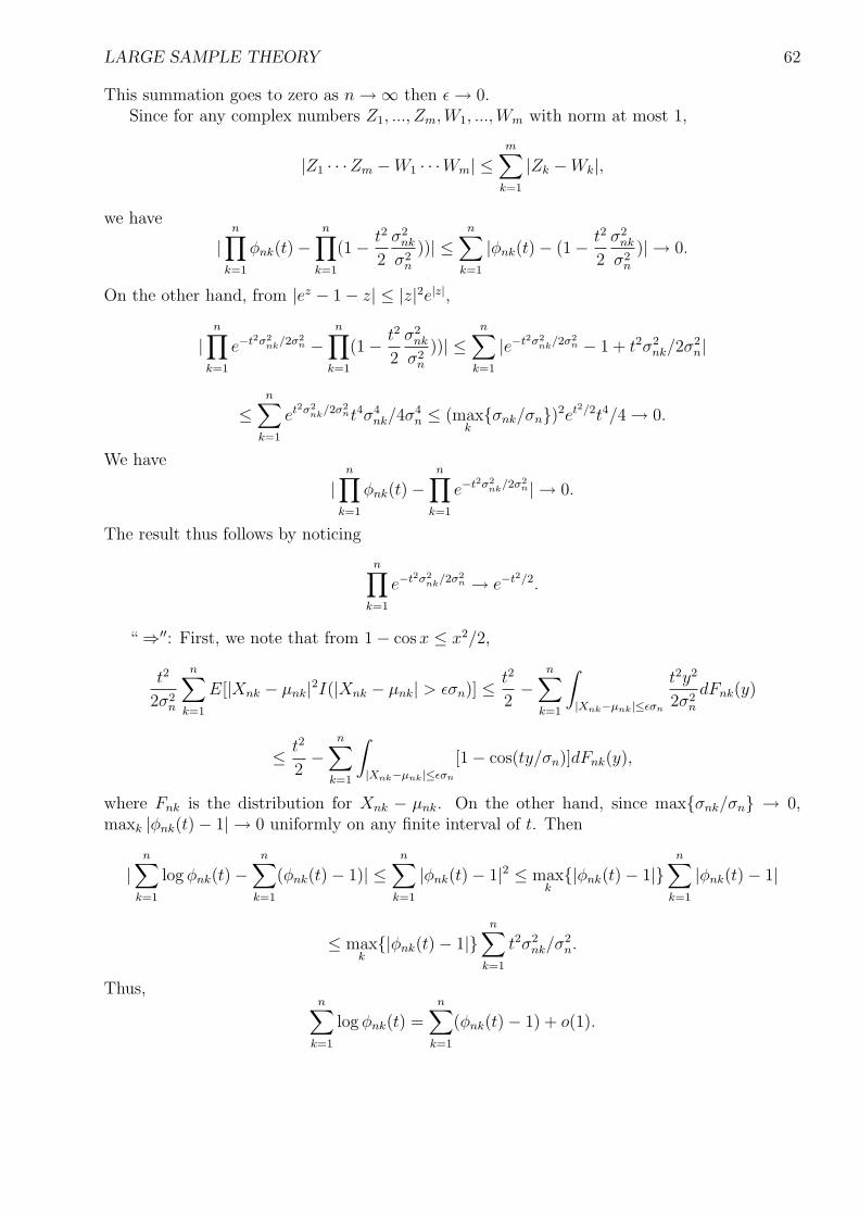
LARGE SAMPLE THEORY 62
This summation goes to zero as n →∞ then ε → 0.Since for any complex numbers Z1, ..., Zm,W1, ..., Wm with norm at most 1,
|Z1 · · ·Zm −W1 · · ·Wm| ≤m∑
k=1
|Zk −Wk|,
we have
|n∏
k=1
φnk(t)−n∏
k=1
(1− t2
2
σ2nk
σ2n
))| ≤n∑
k=1
|φnk(t)− (1− t2
2
σ2nk
σ2n
)| → 0.
On the other hand, from |ez − 1− z| ≤ |z|2e|z|,
|n∏
k=1
e−t2σ2nk/2σ2
n −n∏
k=1
(1− t2
2
σ2nk
σ2n
))| ≤n∑
k=1
|e−t2σ2nk/2σ2
n − 1 + t2σ2nk/2σ
2n|
≤n∑
k=1
et2σ2nk/2σ2
nt4σ4nk/4σ
4n ≤ (max
kσnk/σn)2et2/2t4/4 → 0.
We have
|n∏
k=1
φnk(t)−n∏
k=1
e−t2σ2nk/2σ2
n| → 0.
The result thus follows by noticing
n∏
k=1
e−t2σ2nk/2σ2
n → e−t2/2.
“ ⇒′′: First, we note that from 1− cos x ≤ x2/2,
t2
2σ2n
n∑
k=1
E[|Xnk − µnk|2I(|Xnk − µnk| > εσn)] ≤ t2
2−
n∑
k=1
∫
|Xnk−µnk|≤εσn
t2y2
2σ2n
dFnk(y)
≤ t2
2−
n∑
k=1
∫
|Xnk−µnk|≤εσn
[1− cos(ty/σn)]dFnk(y),
where Fnk is the distribution for Xnk − µnk. On the other hand, since maxσnk/σn → 0,maxk |φnk(t)− 1| → 0 uniformly on any finite interval of t. Then
|n∑
k=1
log φnk(t)−n∑
k=1
(φnk(t)− 1)| ≤n∑
k=1
|φnk(t)− 1|2 ≤ maxk|φnk(t)− 1|
n∑
k=1
|φnk(t)− 1|
≤ maxk|φnk(t)− 1|
n∑
k=1
t2σ2nk/σ
2n.
Thus,n∑
k=1
log φnk(t) =n∑
k=1
(φnk(t)− 1) + o(1).
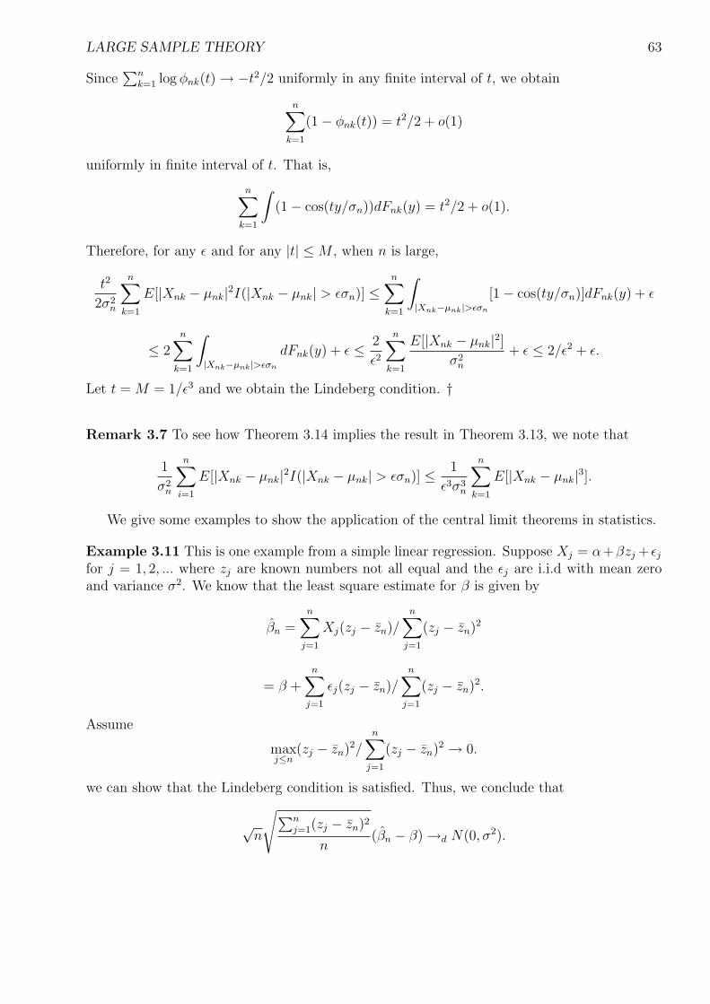
LARGE SAMPLE THEORY 63
Since∑n
k=1 log φnk(t) → −t2/2 uniformly in any finite interval of t, we obtain
n∑
k=1
(1− φnk(t)) = t2/2 + o(1)
uniformly in finite interval of t. That is,
n∑
k=1
∫(1− cos(ty/σn))dFnk(y) = t2/2 + o(1).
Therefore, for any ε and for any |t| ≤ M , when n is large,
t2
2σ2n
n∑
k=1
E[|Xnk − µnk|2I(|Xnk − µnk| > εσn)] ≤n∑
k=1
∫
|Xnk−µnk|>εσn
[1− cos(ty/σn)]dFnk(y) + ε
≤ 2n∑
k=1
∫
|Xnk−µnk|>εσn
dFnk(y) + ε ≤ 2
ε2
n∑
k=1
E[|Xnk − µnk|2]σ2
n
+ ε ≤ 2/ε2 + ε.
Let t = M = 1/ε3 and we obtain the Lindeberg condition. †
Remark 3.7 To see how Theorem 3.14 implies the result in Theorem 3.13, we note that
1
σ2n
n∑i=1
E[|Xnk − µnk|2I(|Xnk − µnk| > εσn)] ≤ 1
ε3σ3n
n∑
k=1
E[|Xnk − µnk|3].
We give some examples to show the application of the central limit theorems in statistics.
Example 3.11 This is one example from a simple linear regression. Suppose Xj = α+βzj + εj
for j = 1, 2, ... where zj are known numbers not all equal and the εj are i.i.d with mean zeroand variance σ2. We know that the least square estimate for β is given by
βn =n∑
j=1
Xj(zj − zn)/n∑
j=1
(zj − zn)2
= β +n∑
j=1
εj(zj − zn)/n∑
j=1
(zj − zn)2.
Assume
maxj≤n
(zj − zn)2/
n∑j=1
(zj − zn)2 → 0.
we can show that the Lindeberg condition is satisfied. Thus, we conclude that
√n
√∑nj=1(zj − zn)2
n(βn − β) →d N(0, σ2).
LARGE SAMPLE THEORY 64
Example 3.12 The example is taken from the randomization test for paired comparison. In apaired study comparing treatment vs control, 2n subjects are grouped into n pairs. For pair, itis decided at random that one subject receives treatment but not the other. Let (Xj, Yj) denotethe values of jth pairs with Xj being the result of the treatment. The usual paired t-test isbased on the normality of Zj = Xj − Yj which may be invalid in practice. The randomizationtest (sometimes called permutation test) avoids this normality assumption, solely based onthe virtue of the randomization that the assignments of the treatment and the control areindependent in the pair, i.e., conditional on |Zj| = zj, Zj = |Zj|sgn(Zj) is independent takingvalues ±|Zj| with probability 1/2, when treatment and control have no difference. Therefore,conditional on z1, z2, ..., the randomization t-test, based on the t-statistic
√n− 1Zn/sz where s2
z
is 1/n∑n
j=1(Zj − Zn)2, has a discrete distribution on 2n equally likely values. We can simulatethis distribution by the Monte Carlo method easily. Then if this statistic is large, there is strongevidence that treatment has large value. When n is large, such computation can be intimate,a better solution is to find an approximation. The Lindeberg-Feller central limit theorem canbe applied if we assume
maxj≤n
z2j /
n∑j=1
z2j → 0.
It can be shown that this statistic has an asymptotic normal distribution N(0, 1). The detailscan be found in Ferguson, page 29.
Example 3.13 In Ferguson, page 30, an example of applying the central limit theorem is givenfor the signed-rank test for paired comparisons. Interested readers can find more details there.
3.3.4 Delta method
In many situation, the statistics are not simply the summation of independent random variablesbut a transformation of the latter. In this case, the Delta method can be used to obtain a similarresult to the central limit theorem.
Theorem 3.15 (Delta method) For random vector X and Xn in Rk , if there exists twoconstant an and µ such that an(Xn−µ) →d X and an →∞, then for any function g : Rk 7→ Rl
such that g has a derivative at µ, denoted by ∇g(µ)
an(g(Xn)− g(µ)) →d ∇g(µ)X.
†
Proof By the Skorohod representation, we can construct Xn and X such that Xn ∼d Xn andX ∼d X (∼d means the same distribution) and an(Xn−µ) →a.s. X. Then an(g(Xn)−g(µ)) →a.s.
∇g(µ)X. We obtain the result. †
As a corollary of Theorem 3.15, if√
n(Xn − µ) →d N(0, σ2), then for any differentiablefunction g(·), √n(g(Xn)− g(µ)) →d N(0, g′(µ)2σ2).
LARGE SAMPLE THEORY 65
Example 3.14 Let X1, X2, ... be i.i.d with fourth moment. An estimate of the sample vari-ance is s2
n = (1/n)∑n
i=1(Xi − Xn)2. We can use the Delta method in deriving the asymp-totic distribution of s2
n. Denote mk as the kth moment of X1 for k ≤ 4. Note that s2n =
(1/n)∑n
i=1 X2i − (
∑ni=1 Xi/n)2 and
√n
[(Xn
(1/n)∑n
i=1 X2i
)−
(m1
m2
)]→d N
(0,
(m2 −m1 m3 −m1m2
m3 −m1m2 m4 −m22
)),
we can apply the Delta method with g(x, y) = y − x2 to obtain
√n(s2
n − V ar(X1)) →d N(0,m4 − (m2 −m21)
2).
Example 3.15 Let (X1, Y1), (X2, Y2), ... be i.i.d bivariate samples with finite fourth moment.One estimate of the correlation among X and Y is
ρn =sxy√s2
xs2y
,
where sxy = (1/n)∑n
i=1(Xi−Xn)(Yi−Yn), s2x = (1/n)
∑ni=1(Xi−Xn)2 and s2
y = (1/n)∑n
i=1(Yi−Yn)2. To derive the large sample distribution of ρn, we can first obtain the large sampledistribution of (sxy, s
2x, s
2y) using the Delta method as in Example 3.14 then further apply the
Delta method with g(x, y, z) = x/√
yz. We skip the details.
Example 3.16 The example is taken from the Pearson’s Chi-square statistic. Suppose thatone subject falls into K categories with probabilities p1, ..., pK , where p1 + ... + pK = 1. Weactually observe n1, ..., nk subjects in these categories from n = n1 + ...+nK i.i.d subjects. ThePearson’s statistic is defined as
χ2 = n
K∑
k=1
(nk
n− pk)
2/pk,
which can be treated as∑
(observed count− expected count)2/expected count. To obtain theasymptotic distribution of χ2, we note that
√n(n1/n − p1, ..., nK/n − pK) has an asymptotic
multivariate normal distribution. Then we can apply the Delta method to g(x1, ..., xK) =∑Ki=1 x2
k.
3.4 Summation of Non-independent Random Variables
In statistical inference, one will also encounter the summation of non-independent randomvariables. Theoretical results of the large sample theory for general non-independent randomvariables do not exist but for some summations with special structure, we have the similarresults to the central limit theorem. These special cases include the U-statistics, the rankstatistics, and the martingales.
LARGE SAMPLE THEORY 66
3.4.1 U-statistics
We suppose X1, ..., Xn are i.i.d. random variables.
Definition 3.6 A U-statistics associated with h(x1, ..., xr) is defined as
Un =1
r!(
nr
)∑
β
h(Xβ1 , ..., Xβr),
where the sum is taken over the set of all unordered subsets β of r different integers chosenfrom 1, ..., n. †
One simple example is h(x, y) = xy. Then Un = (n(n − 1))−1∑
i6=j XiXj. Many examplesof U statistics arise from rank-based statistical inference. If let X(1), ..., X(n) be the orderedrandom variables of X1, ..., Xn, one can see
Un = E[h(X1, ..., Xr)|X(1), ..., X(n)].
Clearly, Un is the summation of non-independent random variables.If define h(x1, ..., xr) as (r!)−1
∑(x1,...,xr) is permutation of (x1, ..., xr) h(x1, ..., xr), then h(x1, ..., xr)
is permutation-symmetric and moreover,
Un =1(nr
)∑
β1<...<βr
h(β1, ..., βr).
In the last expression, h is called the kernel of the U-statistic Un.The following theorem says that the limit distribution of U is the same as the limit distri-
bution of a sum of i.i.d random variables. Thus, the central limit theorem can be applied toU .
Theorem 3.16 Let µ = E[h(X1, ..., Xr)]. If E[h(X1, ..., Xr)2] < ∞, then
√n(Un − µ)−√n
n∑i=1
E[Un − µ|Xi] →p 0.
Consequently,√
n(Un − µ) is asymptotically normal with mean zero and variance r2σ2, where,with X1, ..., Xr, X1, ..., Xr i.i.d variables,
σ2 = Cov(h(X1, X2, ..., Xr), h(X1, X2, ..., Xr)).
†
To prove Theorem 3.16, we need the following lemmas. Let S be a linear space of randomvariables with finite second moments that contain the constants; i.e., 1 ∈ S and for any X, Y ∈S, aX + bY ∈ Sn where a and b are constants. For random variable T , a random variable S iscalled the projection of T on S if E[(T − S)2] minimizes E[(T − S)2], S ∈ S.
Proposition 3.6 Let S be a linear space of random variables with finite second moments.Then S is the projection of T on S if and only if S ∈ S and for any S ∈ S, E[(T − S)S] = 0.
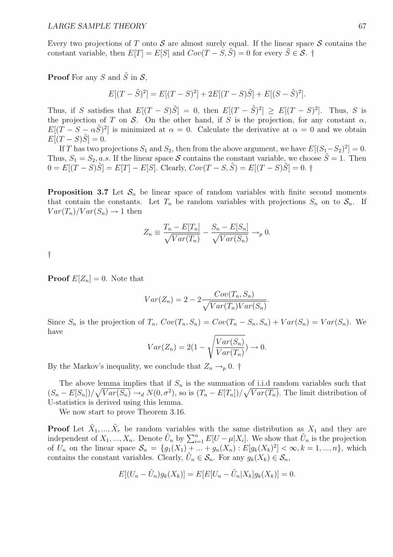
LARGE SAMPLE THEORY 67
Every two projections of T onto S are almost surely equal. If the linear space S contains theconstant variable, then E[T ] = E[S] and Cov(T − S, S) = 0 for every S ∈ S. †
Proof For any S and S in S,
E[(T − S)2] = E[(T − S)2] + 2E[(T − S)S] + E[(S − S)2].
Thus, if S satisfies that E[(T − S)S] = 0, then E[(T − S)2] ≥ E[(T − S)2]. Thus, S isthe projection of T on S. On the other hand, if S is the projection, for any constant α,E[(T − S − αS)2] is minimized at α = 0. Calculate the derivative at α = 0 and we obtainE[(T − S)S] = 0.
If T has two projections S1 and S2, then from the above argument, we have E[(S1−S2)2] = 0.
Thus, S1 = S2, a.s. If the linear space S contains the constant variable, we choose S = 1. Then0 = E[(T − S)S] = E[T ]− E[S]. Clearly, Cov(T − S, S) = E[(T − S)S] = 0. †
Proposition 3.7 Let Sn be linear space of random variables with finite second momentsthat contain the constants. Let Tn be random variables with projections Sn on to Sn. IfV ar(Tn)/V ar(Sn) → 1 then
Zn ≡ Tn − E[Tn]√V ar(Tn)
− Sn − E[Sn]√V ar(Sn)
→p 0.
†
Proof E[Zn] = 0. Note that
V ar(Zn) = 2− 2Cov(Tn, Sn)√
V ar(Tn)V ar(Sn).
Since Sn is the projection of Tn, Cov(Tn, Sn) = Cov(Tn − Sn, Sn) + V ar(Sn) = V ar(Sn). Wehave
V ar(Zn) = 2(1−√
V ar(Sn)
V ar(Tn)) → 0.
By the Markov’s inequality, we conclude that Zn →p 0. †
The above lemma implies that if Sn is the summation of i.i.d random variables such that(Sn −E[Sn])/
√V ar(Sn) →d N(0, σ2), so is (Tn −E[Tn])/
√V ar(Tn). The limit distribution of
U-statistics is derived using this lemma.We now start to prove Theorem 3.16.
Proof Let X1, ..., Xr be random variables with the same distribution as X1 and they areindependent of X1, ..., Xn. Denote Un by
∑ni=1 E[U −µ|Xi]. We show that Un is the projection
of Un on the linear space Sn = g1(X1) + ... + gn(Xn) : E[gk(Xk)2] < ∞, k = 1, ..., n, which
contains the constant variables. Clearly, Un ∈ Sn. For any gk(Xk) ∈ Sn,
E[(Un − Un)gk(Xk)] = E[E[Un − Un|Xk]gk(Xk)] = 0.
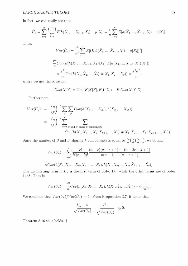
LARGE SAMPLE THEORY 68
In fact, we can easily see that
Un =n∑
i=1
(n−1r−1
)(
nr
) E[h(X1, ..., Xr−1, Xi)− µ|Xi] =r
n
n∑i=1
E[h(X1, ..., Xr−1, Xi)− µ|Xi].
Thus,
V ar(Un) =r2
n2
n∑i=1
E[(E[h(X1, ..., Xr−1, Xi)− µ|Xi])2]
=r2
nCov(E[h(X1, ..., Xr−1, X1)|X1], E[h(X1, ..., Xr−1, X1)|X1])
=r2
nCov(h(X1, X2, ..., Xr), h(X1, X2..., Xr)) =
r2σ2
n,
where we use the equation
Cov(X,Y ) = Cov(E[X|Z], E[Y |Z]) + E[Cov(X, Y |Z)].
Furthermore,
V ar(Un) =
(n
r
)−2 ∑
β
∑
β′Cov(h(Xβ1 , ..., Xβr), h(Xβ′1 , ..., Xβ′r))
=
(n
r
)−2 r∑
k=1
∑
β and β′ share k components
Cov(h(X1, X2, .., Xk, Xk+1, ..., Xr), h(X1, X2, ..., Xk, Xk+1, ..., Xr)).
Since the number of β and β′ sharing k components is equal to(
nr
)(rk
)(n−rr−k
), we obtain
V ar(Un) =r∑
k=1
r!
k!(r − k)!
(n− r)(n− r + 1) · · · (n− 2r + k + 1)
n(n− 1) · · · (n− r + 1)
×Cov(h(X1, X2, .., Xk, Xk+1, ..., Xr), h(X1, X2, ..., Xk, Xk+1, ..., Xr)).
The dominating term in Un is the first term of order 1/n while the other terms are of order1/n2. That is,
V ar(Un) =r2
nCov(h(X1, X2, ..., Xr), h(X1, X2, ..., Xr)) + O(
1
n2).
We conclude that V ar(Un)/V ar(Un) → 1. From Proposition 3.7, it holds that
Un − µ√V ar(Un)
− Un√V ar(Un)
→p 0.
Theorem 3.16 thus holds. †
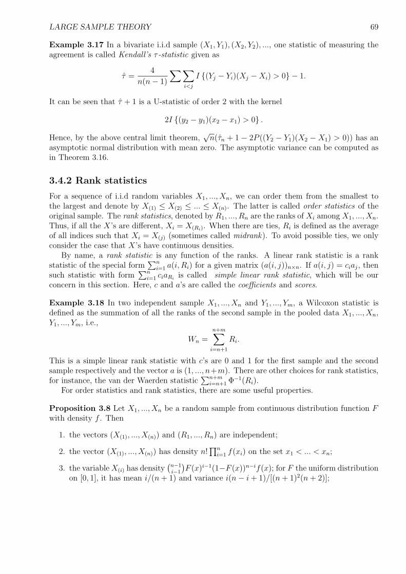
LARGE SAMPLE THEORY 69
Example 3.17 In a bivariate i.i.d sample (X1, Y1), (X2, Y2), ..., one statistic of measuring theagreement is called Kendall’s τ -statistic given as
τ =4
n(n− 1)
∑∑i<j
I (Yj − Yi)(Xj −Xi) > 0 − 1.
It can be seen that τ + 1 is a U-statistic of order 2 with the kernel
2I (y2 − y1)(x2 − x1) > 0 .
Hence, by the above central limit theorem,√
n(τn + 1 − 2P ((Y2 − Y1)(X2 −X1) > 0)) has anasymptotic normal distribution with mean zero. The asymptotic variance can be computed asin Theorem 3.16.
3.4.2 Rank statistics
For a sequence of i.i.d random variables X1, ..., Xn, we can order them from the smallest tothe largest and denote by X(1) ≤ X(2) ≤ ... ≤ X(n). The latter is called order statistics of theoriginal sample. The rank statistics, denoted by R1, ..., Rn are the ranks of Xi among X1, ..., Xn.Thus, if all the X’s are different, Xi = X(Ri). When there are ties, Ri is defined as the averageof all indices such that Xi = X(j) (sometimes called midrank). To avoid possible ties, we onlyconsider the case that X’s have continuous densities.
By name, a rank statistic is any function of the ranks. A linear rank statistic is a rankstatistic of the special form
∑ni=1 a(i, Ri) for a given matrix (a(i, j))n×n. If a(i, j) = ciaj, then
such statistic with form∑n
i=1 ciaRiis called simple linear rank statistic, which will be our
concern in this section. Here, c and a’s are called the coefficients and scores.
Example 3.18 In two independent sample X1, ..., Xn and Y1, ..., Ym, a Wilcoxon statistic isdefined as the summation of all the ranks of the second sample in the pooled data X1, ..., Xn,Y1, ..., Ym, i.e.,
Wn =n+m∑
i=n+1
Ri.
This is a simple linear rank statistic with c’s are 0 and 1 for the first sample and the secondsample respectively and the vector a is (1, ..., n+m). There are other choices for rank statistics,for instance, the van der Waerden statistic
∑n+mi=n+1 Φ−1(Ri).
For order statistics and rank statistics, there are some useful properties.
Proposition 3.8 Let X1, ..., Xn be a random sample from continuous distribution function Fwith density f . Then
1. the vectors (X(1), ..., X(n)) and (R1, ..., Rn) are independent;
2. the vector (X(1), ..., X(n)) has density n!∏n
i=1 f(xi) on the set x1 < ... < xn;
3. the variable X(i) has density(
n−1i−1
)F (x)i−1(1−F (x))n−if(x); for F the uniform distribution
on [0, 1], it has mean i/(n + 1) and variance i(n− i + 1)/[(n + 1)2(n + 2)];
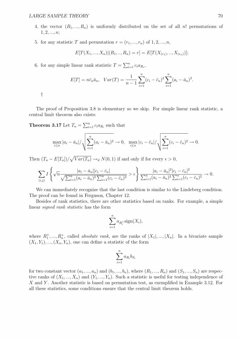
LARGE SAMPLE THEORY 70
4. the vector (R1, ..., Rn) is uniformly distributed on the set of all n! permutations of1, 2, ..., n;
5. for any statistic T and permutation r = (r1, ..., rn) of 1, 2, ..., n,
E[T (X1, ..., Xn)|(R1, .., Rn) = r] = E[T (X(r1), .., X(rn))];
6. for any simple linear rank statistic T =∑n
i=1 ciaRi,
E[T ] = ncnan, V ar(T ) =1
n− 1
n∑i=1
(ci − cn)2
n∑i=1
(ai − an)2.
†
The proof of Proposition 3.8 is elementary so we skip. For simple linear rank statistic, acentral limit theorem also exists:
Theorem 3.17 Let Tn =∑n
i=1 ciaRisuch that
maxi≤n
|ai − an|/√√√√
n∑i=1
(ai − an)2 → 0, maxi≤n
|ci − cn|/√√√√
n∑i=1
(ci − cn)2 → 0.
Then (Tn − E[Tn])/√
V ar(Tn) →d N(0, 1) if and only if for every ε > 0,
∑
(i,j)
I
√
n|ai − an||ci − cn|√∑n
i=1(ai − an)2∑n
i=1(ci − cn)2> ε
|ai − an|2|ci − cn|2∑n
i=1(ai − an)2∑n
i=1(ci − cn)2→ 0.
We can immediately recognize that the last condition is similar to the Lindeberg condition.The proof can be found in Ferguson, Chapter 12.
Besides of rank statistics, there are other statistics based on ranks. For example, a simplelinear signed rank statistic has the form
n∑i=1
aR+isign(Xi),
where R+1 , ..., R+
n , called absolute rank, are the ranks of |X1|, ..., |Xn|. In a bivariate sample(X1, Y1), ..., (Xn, Yn), one can define a statistic of the form
n∑i=1
aRibSi
for two constant vector (a1, ..., an) and (b1, ..., bn), where (R1, ..., Rn) and (S1, ..., Sn) are respec-tive ranks of (X1, ..., Xn) and (Y1, ..., Yn). Such a statistic is useful for testing independence ofX and Y . Another statistic is based on permutation test, as exemplified in Example 3.12. Forall these statistics, some conditions ensure that the central limit theorem holds.
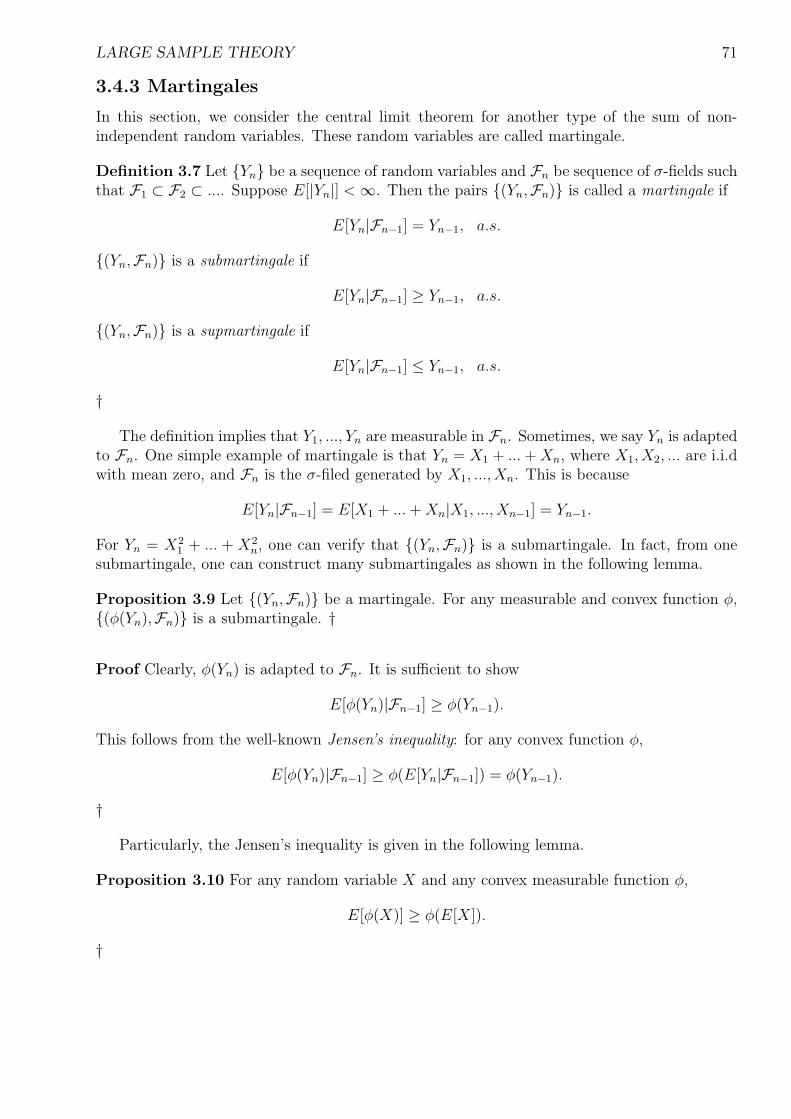
LARGE SAMPLE THEORY 71
3.4.3 Martingales
In this section, we consider the central limit theorem for another type of the sum of non-independent random variables. These random variables are called martingale.
Definition 3.7 Let Yn be a sequence of random variables and Fn be sequence of σ-fields suchthat F1 ⊂ F2 ⊂ .... Suppose E[|Yn|] < ∞. Then the pairs (Yn,Fn) is called a martingale if
E[Yn|Fn−1] = Yn−1, a.s.
(Yn,Fn) is a submartingale if
E[Yn|Fn−1] ≥ Yn−1, a.s.
(Yn,Fn) is a supmartingale if
E[Yn|Fn−1] ≤ Yn−1, a.s.
†
The definition implies that Y1, ..., Yn are measurable in Fn. Sometimes, we say Yn is adaptedto Fn. One simple example of martingale is that Yn = X1 + ... + Xn, where X1, X2, ... are i.i.dwith mean zero, and Fn is the σ-filed generated by X1, ..., Xn. This is because
E[Yn|Fn−1] = E[X1 + ... + Xn|X1, ..., Xn−1] = Yn−1.
For Yn = X21 + ... + X2
n, one can verify that (Yn,Fn) is a submartingale. In fact, from onesubmartingale, one can construct many submartingales as shown in the following lemma.
Proposition 3.9 Let (Yn,Fn) be a martingale. For any measurable and convex function φ,(φ(Yn),Fn) is a submartingale. †
Proof Clearly, φ(Yn) is adapted to Fn. It is sufficient to show
E[φ(Yn)|Fn−1] ≥ φ(Yn−1).
This follows from the well-known Jensen’s inequality: for any convex function φ,
E[φ(Yn)|Fn−1] ≥ φ(E[Yn|Fn−1]) = φ(Yn−1).
†
Particularly, the Jensen’s inequality is given in the following lemma.
Proposition 3.10 For any random variable X and any convex measurable function φ,
E[φ(X)] ≥ φ(E[X]).
†
LARGE SAMPLE THEORY 72
Proof We first claim that for any x0, there exists a constant k0 such that for any x,
φ(x) ≥ φ(x0) + k0(x− x0).
The line φ(x0) + k0(x − x0) is called the supporting line for φ(x) at x0. By the convexity, wehave that for any x′ < y′ < x0 < y < x,
φ(x0)− φ(x′)x0 − x′
≤ φ(y)− φ(x0)
y − x0
≤ φ(x)− φ(x0)
x− x0
.
Thus, φ(x)−φ(x0)x−x0
is bounded and decreasing as x decreases to x0. Let the limit be k+0 then
φ(x)− φ(x0)
x− x0
≥ k+0 .
I.e.,φ(x) ≥ k+
0 (x− x0) + φ(x0).
Similarly,φ(x′)− φ(x0)
x′ − x0
≤ φ(y′)− φ(x0)
y′ − x0
≤ φ(x)− φ(x0)
x− x0
.
Then φ(x′)−φ(x0)x′−x0
is increasing and bounded as x′ increases to x0. Let the limit be k−0 then
φ(x′) ≥ k−0 (x′ − x0) + φ(x0).
Clearly, k+0 ≥ k−0 . Combining those two inequalities, we obtain
φ(x) ≥ φ(x0) + k0(x− x0)
for k0 = (k+0 + k−0 )/2. We choose x0 = E[X] then
φ(X) ≥ φ(E[X]) + k0(X − E[X]).
The Jensen’s inequality holds by taking the expectation on both sides. †
If (Yn,Fn) is a submartingale, we can write Yn = (Yn − E[Yn|Fn−1]) + E[Yn|Fn−1]. Notethat (Yn−E[Yn|Fn−1],Fn) is a martingale and that E[Yn|Fn−1] is measurable in Fn−1. Thusany submartingale can be written as the summation of a martingale and a random variablepredictable in Fn−1. We now state the limit theorems for the martingales.
Theorem 3.18 (Martingale Convergence Theorem) Let (Xn,Fn) be submartingale. IfK = supn E[|Xn|] < ∞, then Xn →a.s. X where X is a random variable satisfying E[|X|] ≤ K.†
The proof needs the maximal inequality for a submartingale and the up-crossing inequality.
Proof We first prove the following maximal inequality: for α > 0,
P (maxi≤n
Xi ≥ α) ≤ 1
αE[|Xn|].
LARGE SAMPLE THEORY 73
To see that, we note that
P (maxi≤n
Xi ≥ α)
=n∑
i=1
P (X1 < α, ..., Xi−1 < α,Xi ≥ α)
≤n∑
i=1
E[I(X1 < α, ..., Xi−1 < α,Xi ≥ α)Xi
α]
=1
α
n∑i=1
E[I(X1 < α, ..., Xi−1 < α,Xi ≥ α)Xi].
Since E[Xn|X1, ..., Xn−1] ≥ Xn−1, E[Xn|X1, ..., Xn−2] ≥ E[Xn−1|X1, ..., Xn−2] and so on. Weobtain E[Xn|X1, ..., Xi] ≥ E[Xi+1|X1, ..., Xi] ≥ Xi for i = 1, ..., n− 1. Thus,
P (maxi≤n
Xi ≥ α) ≤ 1
α
n∑i=1
E[I(X1 < α, ..., Xi−1 < α, Xi ≥ α)E[Xn|X1, ..., Xi]]
≤ 1
αE[Xn
n∑i=1
I(X1 < α, ..., Xi−1 < α, Xi ≥ α)] ≤ 1
αE[Xn] ≤ 1
αE[|Xn|].
For any interval [α, β] (α < β), we define a sequence of numbers τ1, τ2, ... as follows:τ1 is the smallest j such that 1 ≤ j ≤ n and Xj ≤ α and is n if there is not such j;τ2k is the smallest j such that τ2k−1 < j ≤ n and Xj ≥ β, and is n if there is not such j;τ2k+1 is the smallest j such τ2k < j ≤ n and Xj ≤ α, and is n if there is not such j.A random variable U , called upcrossings of [α, β] by X1, ..., Xn, is the largest i such thatXτ2i−1
≤ α < β ≤ Xτ2i. We then show that
E[U ] ≤ E[|Xn|] + |α|β − α
.
Let Yk = max0, Xk − α and θ = β − α. It is easy to see Y1, ..., Yn is a submartingale. The τk
are unchanged if the definitions Xj ≤ α is replaced by Yj = 0 and Xj ≥ β by Yj ≥ θ, and so Uis also the number of upcrossings of [0, θ] by Y1, .., Yn. We also obtain
E[Yτ2k+1− Yτ2k
] =∑
1≤k1<k2≤n
E[(Yk2 − Yk1)I(τ2k+1 = k2, τ2k = k1)]
=n−1∑
k1=1
n∑
k′=2
E[I(τ2k = k1, k1 < k′ ≤ τ2k+1)(Yk′ − Yk′−1)]
=n−1∑
k1=1
n∑
k′=2
E[I(τ2k = k1, k1 < k′)(1− I(τ2k+1 < k′))(Yk′ − Yk′−1)].
By the definition, if τ2k−1 = i is measurable in Fi for i = 1, ..., n, where Fi is the σ-fieldgenerated by Y1, ..., Yi, then
τ2k = j = ∪j−1i=1 τ2k−1 = i, Yi+1 < θ, ..., Yj−1 ≤ θ, Yj ≥ θ
LARGE SAMPLE THEORY 74
belongs to the σ-field Fj and τ2k = n = τ2k ≤ n− 1c lies in Fn. Similarly, if τ2k = i ∈ Fi
for any i = 1, ..., n, so is τ2k+1 = i ∈ Fi for any i = 1, ..., n. Thus, by the deduction, weobtain that for any i = 1, ..., n, τk = i is in Fi. Then,
E[I(τ2k = k1, k1 < k′)(1− I(τ2k+1 < k′))(Yk′ − Yk′−1)]
= E[I(τ2k = k1, k1 < k′)(1− I(τ2k+1 < k′))(E[Yk′|Fk′−1]− Yk′−1)] ≥ 0.
We conclude that E[Yτ2k+1− Yτ2k
] ≥ 0.Since τk is strictly increasing and τn = n,
Yn = Yτn ≥ Yτn − Yτ1 =n∑
k=2
(Yτk− Yτk−1
) =∑
2≤k≤n,k even
(Yτk− Yτk−1
) +∑
2≤k≤n,k odd
(Yτk− Yτk−1
).
When k is even, Yτk− Yτk−1 ≥ θ and the total number of such k is U . The expectation of the
second half is non-negative. We obtain
E[Yn] ≥ θE[U ].
Thus,
E[U ] ≤ θ
E[Yn] ≤ E[|X|+ |α|
β − α.
With the maximal inequality, we can start to prove the martingale convergence theorem.Let Un be the number of upcrossings of [α, β] by X1, ..., Xn. Then
E[Un] ≤ K + |α|β − α
.
Let X∗ = lim supn Xn and X∗ = lim infn Xn. If X∗ < α < β < X∗, then Un must go to infinity.Since Un is bounded with probability 1, P (X∗ < α < β < X∗) = 0. Now
X∗ < X∗ = ∪α<β,α,β are rational numbersX∗ < α < β < X∗.We obtain P (X∗ = X∗) = 1. That is, Xn converges to their common values X. By the Fatou’slemma, E[|X|] ≤ lim infn E[|Xn|] ≤ K. X is integrable and finite with probability 1. † .
As a corollary of the martingale convergence theorem, we obtain
Corollary 3.1 If Fn is increasing σ-field and denote F∞ as the σ-field generated by ∪∞n=1Fn,then for any random variable Z with E[|Z|] < ∞, it holds
E[Z|Fn] →a.s. E[Z|F∞].
†
Proof Denote Yn = E[Zn|Fn]. Clearly, Yn is a martingale adapted to Fn. Moreover, E[|Yn|] ≤E[|Z|]. By the martingale convergence theorem, Yn converges to some random variable Y almostsurely. Clearly, Y is measurable in F∞. We then show Yn is uniformly integrable. SinceYn ≤ E[|Zn||Fn], we may assume Z is non-negative. For any ε > 0, there exists a δ such
LARGE SAMPLE THEORY 75
that E[ZIA] < ε whenever P (A) < δ (since the measure E[ZIA] is absolutely continuous withrespect to the measure P ). Note that for a large α, consider the set A = P (E[Z|Fn] ≥ α).Since
P (A) = E[I(E[Z|Fn] ≥ α)] ≤ 1
αE[Z],
we can choose α large enough (independent of n) such that P (A) < δ. Thus, E[ZI(E[Z|Fn] ≥α)] < ε for any n. We conclude E[Z|Fn] is uniformly integrable. With the uniform integrability,we have that for any A ∈ Fk, limn
∫A
YndP =∫
AY dP. Note that
∫A
YndP =∫
AZdP for n > k.
Thus,∫
AY dP =
∫A
ZdP =∫
AE[Z|F∞]dP . This is true for any A ∈ ∪∞n=1F∞ so it is also true
for any A ∈ F∞. Since Y is measurable in F∞, Y = E[Z|F∞], a.s. †
Finally, a similar theorem to the Lindeberg-Feller central limit theorem also exists for themartingales.
Theorem 3.19 (Martingale Central Limit Theorem) Let (Yn1,Fn1), (Yn2,Fn2), ... be amartingale. Define Xnk = Ynk − Yn,k−1 with Yn0 = 0 thus Ynk = Xn1 + ... + Xnk. Suppose that
∑
k
E[X2nk|Fn,k−1] →p σ2
where σ is a positive constant and that
∑
k
E[X2nkI(|Xnk| ≥ ε)|Fn,k−1] →p 0
for each ε > 0. Then ∑
k
Xnk →d N(0, σ2).
†
The proof is based on the approximation of the characteristic function and we skip thedetails here.
3.5 Some Notation
In a probability space (Ω,A, P ), let Xn be random variables (random vectors). We introducethe following notation: Xn = op(1) denotes that Xn converges in probability to zero, Xn = Op(1)denotes that Xn is bounded in probability; i.e.,
limM→∞
lim supn
P (|Xn| ≥ M) = 0.
It is easy to see Xn = Op(1) is equivalent to saying Xn is uniformly tight. Furthermore, fora sequence of random variable rn, Xn = op(rn) means that |Xn|/rn →p 0 and Xn = Op(rn)means that |Xn|/rn is bounded in probability.
There are many rules of calculus with o and O symbols. For instance, some commonly usedformulae are (Rn is a deterministic sequence)
op(1) + op(1) = op(1), Op(1) + Op(1) = Op(1), Op(1)op(1) = op(1),
LARGE SAMPLE THEORY 76
(1 + op(1))−1 = 1 + op(1), op(Rn) = Rnop(1), Op(Rn) = RnOp(1),
op(Op(1)) = op(1).
Furthermore, if a real function R(·) satisfies that R(h) = o(|h|p) as h → 0, then R(Xn) =op(|Xn|p); if R(h) = O(|h|p) as h → 0, then R(Xn) = Op(|Xn|p). Readers should be able toprove these results without difficulty.
READING MATERIALS : You should read Lehmann and Casella, Section 1.8, Ferguson, Part1, Part 2, Part 3 12-15
PROBLEMS
1. (a) If X1, X2, ... are i.i.d N(0, 1), then X(n)/√
2 log n →p 1 where X(n) is the maximumof X1, ..., Xn. Hint: use the following inequality: for any δ > 0,
δ√2π
e−(1+δ)y2/2y ≤∫ ∞
y
1√2π
e−x2/2dx ≤ e−y2(1−δ)/2
√δ
.
(b) If X1, X2, ... are i.i.d Uniform(0, 1), derive the limit distribution of n(1−X(n)).
2. Suppose that U ∼ Uniform(0, 1), α > 0, and
Xn = (nα/ log(n + 1))I[0,n−α](U).
(a) Show that Xn →a.s. 0 and E[Xn] → 0.
(b) Can you find a random variable Y with |Xn| ≤ Y for all n with E[Y ] < ∞?
(c) For what values of α does the uniform integrability condition
lim supn→∞
E[|Xn|I|Xn|≥M ] → 0, as M →∞
hold?
3. (a) Show by example that distribution functions having densities can converge in distri-bution even if the densities do not converge. Hint: Consider fn(x) = 1 + cos 2πnxin [0, 1].
(b) Show by example that distributions with densities can converge in distribution to alimit that has no density.
(c) Show by example that discrete distributions can converge in distribution to a limitthat has a density.
4. Stirling’s formula. Let Sn = X1 + ...+Xn, where the X1, ..., Xn are independent and eachhas the Poisson distribution with parameters 1. Calculate or prove successively:
LARGE SAMPLE THEORY 77
(a) Calculate the expectation of (Sn − n)/√
n−, the negative part of (Sn − n)/√
n.
(b) Show (Sn − n)/√
n− →d Z−, where Z has a standard normal distribution.
(c) Show
E
[Sn − n√
n
−]→ E[Z−].
(d) Use the above results to derive the Stirling’s formula:
n! ∼√
2πnn+1/2e−n.
5. This problem gives an alternative way of proving the Slutsky theorem. Let Xn →d Xand Yn →p y for some constant y. Assume Xn and Yn are both measurable functionson the same probability measure space (Ω,A, P ). Then (Xn, Yn)′ can be considered as abivariate random variable into R2.
(a) Show (Xn, Yn)′ →d (X, y)′. Hint: show the characteristic function of (Xn, Yn)′ con-verges using the dominated convergence theorem.
(b) Use the continuous mapping theorem to prove the Slutsky theorem. Hint: first showZnXn →d zX using the function g(x, z) = xz; then show ZnXn + Yn →d zX + yusing the function g(x, y) = x + y.
6. Suppose that Xn is a sequence of random variables in a probability measure space.Show that, if E[g(Xn)] → E[g(X)] for all continuous g with bounded support (that is,g(x) is zero when x is outside a bounded interval), then Xn →d X. Hint: verify (c) of thePortmanteau Theorem. Follow the proof for (c) by considering g(x) = 1− ε/[ε+d(x,Gc∪(−M, M)c)] for any M .
7. Suppose that X1, ..., Xn are i.i.d with distribution function G(x). Let Mn = maxX1, .., Xn.(a) If G(x) = (1− exp−αx)I(x > 0), what is the limit distribution of Mn−α−1 log n?
(b) If
G(x) =
0 if x ≤ 1,1− x−α if x ≥ 1,
where α > 0, what is the limit distribution of n−1/αMn?
(c) If
G(x) =
0 if x ≤ 0,1− (1− x)α if 0 ≤ x ≤ 1,1 if x ≥ 1,
where α > 0, what is the limit distribution of n1/α(Mn − 1)?
8. (a) Suppose that X1, X2, ... are i.i.d in R2 with distribution giving probability θ1 to (1, 0),probability θ2 to (0, 1), θ3 to (0, 0) and θ4 to (−1,−1) where θj ≥ 0 for j = 1, 2, 3, 4and θ1 + ...+ θ4 = 1. Find the limiting distribution of
√n(Xn−E[X1]) and describe
the resulting approximation to the distribution of Xn.
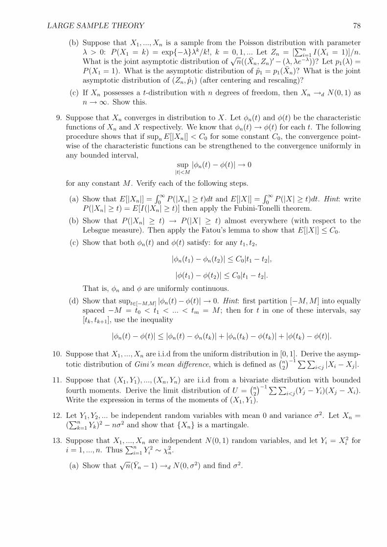
LARGE SAMPLE THEORY 78
(b) Suppose that X1, ..., Xn is a sample from the Poisson distribution with parameterλ > 0: P (X1 = k) = exp−λλk/k!, k = 0, 1, ... Let Zn = [
∑ni=1 I(Xi = 1)]/n.
What is the joint asymptotic distribution of√
n((Xn, Zn)′− (λ, λe−λ))? Let p1(λ) =P (X1 = 1). What is the asymptotic distribution of p1 = p1(Xn)? What is the jointasymptotic distribution of (Zn, p1) (after centering and rescaling)?
(c) If Xn possesses a t-distribution with n degrees of freedom, then Xn →d N(0, 1) asn →∞. Show this.
9. Suppose that Xn converges in distribution to X. Let φn(t) and φ(t) be the characteristicfunctions of Xn and X respectively. We know that φn(t) → φ(t) for each t. The followingprocedure shows that if supn E[|Xn|] < C0 for some constant C0, the convergence point-wise of the characteristic functions can be strengthened to the convergence uniformly inany bounded interval,
sup|t|<M
|φn(t)− φ(t)| → 0
for any constant M . Verify each of the following steps.
(a) Show that E[|Xn|] =∫∞
0P (|Xn| ≥ t)dt and E[|X|] =
∫∞0
P (|X| ≥ t)dt. Hint: writeP (|Xn| ≥ t) = E[I(|Xn| ≥ t)] then apply the Fubini-Tonelli theorem.
(b) Show that P (|Xn| ≥ t) → P (|X| ≥ t) almost everywhere (with respect to theLebsgue measure). Then apply the Fatou’s lemma to show that E[|X|] ≤ C0.
(c) Show that both φn(t) and φ(t) satisfy: for any t1, t2,
|φn(t1)− φn(t2)| ≤ C0|t1 − t2|,|φ(t1)− φ(t2)| ≤ C0|t1 − t2|.
That is, φn and φ are uniformly continuous.
(d) Show that supt∈[−M,M ] |φn(t)− φ(t)| → 0. Hint: first partition [−M,M ] into equallyspaced −M = t0 < t1 < ... < tm = M ; then for t in one of these intervals, say[tk, tk+1], use the inequality
|φn(t)− φ(t)| ≤ |φn(t)− φn(tk)|+ |φn(tk)− φ(tk)|+ |φ(tk)− φ(t)|.
10. Suppose that X1, ..., Xn are i.i.d from the uniform distribution in [0, 1]. Derive the asymp-
totic distribution of Gini’s mean difference, which is defined as(
n2
)−1 ∑∑i<j |Xi −Xj|.
11. Suppose that (X1, Y1), ..., (Xn, Yn) are i.i.d from a bivariate distribution with bounded
fourth moments. Derive the limit distribution of U =(
n2
)−1 ∑∑i<j(Yj − Yi)(Xj − Xi).
Write the expression in terms of the moments of (X1, Y1).
12. Let Y1, Y2, ... be independent random variables with mean 0 and variance σ2. Let Xn =(∑n
k=1 Yk)2 − nσ2 and show that Xn is a martingale.
13. Suppose that X1, ..., Xn are independent N(0, 1) random variables, and let Yi = X2i for
i = 1, ..., n. Thus∑n
i=1 Y 2i ∼ χ2
n.
(a) Show that√
n(Yn − 1) →d N(0, σ2) and find σ2.
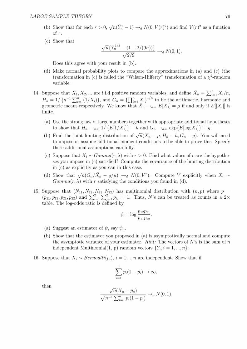
LARGE SAMPLE THEORY 79
(b) Show that for each r > 0,√
n(Y rn − 1) →d N(0, V (r)2) and find V (r)2 as a function
of r.
(c) Show that √nY 1/3
n − (1− 2/(9n))√2/9
→d N(0, 1).
Does this agree with your result in (b).
(d) Make normal probability plots to compare the approximations in (a) and (c) (thetransformation in (c) is called the “Wilson-Hilferty” transformation of a χ2-randomvariable.
14. Suppose that X1, X2, ... are i.i.d positive random variables, and define Xn =∑n
i=1 Xi/n,
Hn = 1/ n−1∑n
i=1(1/Xi), and Gn = ∏ni=1 Xi1/n
to be the arithmetic, harmonic andgeometric means respectively. We know that Xn →a.s. E[X1] = µ if and only if E[|Xi|] isfinite.
(a) Use the strong law of large numbers together with appropriate additional hypothesesto show that Hn →a.s. 1/ E[1/X1] ≡ h and Gn →a.s. expE[log X1] ≡ g.
(b) Find the joint limiting distribution of√
n(Xn − µ,Hn − h,Gn − g). You will needto impose or assume additional moment conditions to be able to prove this. Specifythese additional assumptions carefully.
(c) Suppose that Xi ∼ Gamma(r, λ) with r > 0. Find what values of r are the hypothe-ses you impose in (c) satisfied? Compute the covariance of the limiting distributionin (c) as explicitly as you can in this case.
(d) Show that√
n(Gn/Xn − g/µ) →d N(0, V 2). Compute V explicitly when Xi ∼Gamma(r, λ) with r satisfying the conditions you found in (d).
15. Suppose that (N11, N12, N21, N22) has multinomial distribution with (n, p) where p =(p11, p12, p21, p22) and
∑2i=1
∑2j=1 pij = 1. Thus, N ’s can be treated as counts in a 2×
table. The log-odds ratio is defined by
ψ = logp12p21
p11p22
.
(a) Suggest an estimator of ψ, say ψn.
(b) Show that the estimator you proposed in (a) is asymptotically normal and computethe asymptotic variance of your estimator. Hint: The vectors of N ’s is the sum of nindependent Multinomial(1, p) random vectors Yi, i = 1, ..., n.
16. Suppose that Xi ∼ Bernoulli(pi), i = 1, .., n are independent. Show that if
n∑i=1
pi(1− pi) →∞,
then √n(Xn − pn)√
n−1∑n
i=1 pi(1− pi)→d N(0, 1).
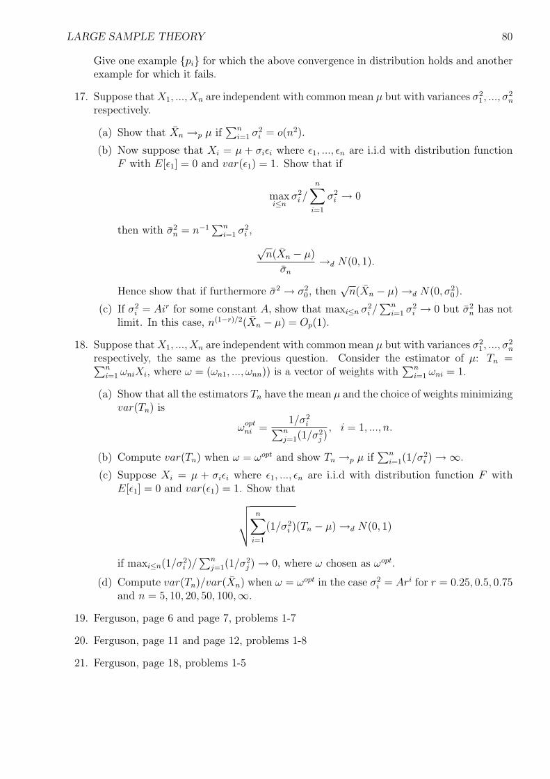
LARGE SAMPLE THEORY 80
Give one example pi for which the above convergence in distribution holds and anotherexample for which it fails.
17. Suppose that X1, ..., Xn are independent with common mean µ but with variances σ21, ..., σ
2n
respectively.
(a) Show that Xn →p µ if∑n
i=1 σ2i = o(n2).
(b) Now suppose that Xi = µ + σiεi where ε1, ..., εn are i.i.d with distribution functionF with E[ε1] = 0 and var(ε1) = 1. Show that if
maxi≤n
σ2i /
n∑i=1
σ2i → 0
then with σ2n = n−1
∑ni=1 σ2
i ,
√n(Xn − µ)
σn
→d N(0, 1).
Hence show that if furthermore σ2 → σ20, then
√n(Xn − µ) →d N(0, σ2
0).
(c) If σ2i = Air for some constant A, show that maxi≤n σ2
i /∑n
i=1 σ2i → 0 but σ2
n has notlimit. In this case, n(1−r)/2(Xn − µ) = Op(1).
18. Suppose that X1, ..., Xn are independent with common mean µ but with variances σ21, ..., σ
2n
respectively, the same as the previous question. Consider the estimator of µ: Tn =∑ni=1 ωniXi, where ω = (ωn1, ..., ωnn)) is a vector of weights with
∑ni=1 ωni = 1.
(a) Show that all the estimators Tn have the mean µ and the choice of weights minimizingvar(Tn) is
ωoptni =
1/σ2i∑n
j=1(1/σ2j )
, i = 1, ..., n.
(b) Compute var(Tn) when ω = ωopt and show Tn →p µ if∑n
i=1(1/σ2i ) →∞.
(c) Suppose Xi = µ + σiεi where ε1, ..., εn are i.i.d with distribution function F withE[ε1] = 0 and var(ε1) = 1. Show that
√√√√n∑
i=1
(1/σ2i )(Tn − µ) →d N(0, 1)
if maxi≤n(1/σ2i )/
∑nj=1(1/σ
2j ) → 0, where ω chosen as ωopt.
(d) Compute var(Tn)/var(Xn) when ω = ωopt in the case σ2i = Ari for r = 0.25, 0.5, 0.75
and n = 5, 10, 20, 50, 100,∞.
19. Ferguson, page 6 and page 7, problems 1-7
20. Ferguson, page 11 and page 12, problems 1-8
21. Ferguson, page 18, problems 1-5

LARGE SAMPLE THEORY 81
22. Ferguson, page 23, page 24 and page 25, problems 1-8
23. Ferguson, page 34 and page 35, problems 1-10
24. Ferguson, page 42 and page 43, problems 1-6
25. Ferguson, page 49 and page 50, problems 1-6
26. Ferguson, page 54 and page 55, problems 1-4
27. Ferguson, page 60, problems 1-4
28. Ferguson, page 65 and page 66, problems 1-3
29. Read Ferguson, pages 87-92 and do problems 3-6
30. Ferguson, page 100, problems 1-2
31. Lehmann and Casella, page 75, problems 8.2, 8.3
32. Lehmann and Casella, page 76, problems 8.8, 8.10, 8.11, 8.12, 8.14, 8.15, 8.16, 8.17 8.18
33. Lehmann and Casella, page 77, problems 8.19, 8.20, 8.21, 8.22, 8.23, 8.24, 8.25, 8.26
POINT ESTIMATION AND EFFICIENCY 82
CHAPTER 4 POINT ESTIMATION AND EFFICIENCY
The objective of science is to make general conclusions based on observed empirical data orphenomenon. The differences among different scientific areas are scientific tools implementedand scientific approaches to derive the decisions. However, they follow a similar procedure asfollows:(A) a class of mathematical models is proposed to model scientific phenomena or processes;(B) an estimated model is derived using the empirical data;(C) the obtained model is validated using more and new observations; if wrong, go back to (A).Usually, in (A), the class of mathematical models is proposed based on either past experienceor some physical laws. (B) is the step where all different scientific tools can play by using math-ematical methods to determine the model. (C) is the step of model validation. Undoubtedlyeac step is important.
In statistical science, (A) corresponds to proposing a class of distribution functions, denotedby P , to describe the probabilistic mechanisms of data generation. (B) consists of all kinds ofstatistical methods to decide which distribution in the class of (A) fits the data best. (C) ishow one can validate or test the goodness of the distribution obtained in (B). Our goal of thiscourse is mainly on (B), which is called statistical inference step.
One good estimation approach should be able to estimate model parameters with reasonableaccuracy. Such accuracy is characterized by either unbiasedness in finite sample performance orconsistency in large sample performance. Furthermore, by accounting for randomness in datageneration, we also want the estimation to be somewhat robust to intrinsic random mechanism.This robustness is characterized by the variance of the estimates. Thus, an ideally best estimatorshould have no bias and have the smallest variance in any finite sample. Unfortunately, althoughsuch estimators may exist for some models, most of models do not. One compromise is to seekan estimator which has no bias and has the smallest variance in large sample, i.e., an estimatewhich is asymptotically unbiased and efficient. Fortunately, such an estimator exists for mostof models.
In this chapter, we review some commonly-used estimation approaches, with particularattention to the estimation providing the unbiased and smallest variance estimators if they exist.The smallest variance for finite sample is characterized by the Cramer-Rao bound (efficiencybound in finite sample). Such a bound also turns out to be the efficiency bound in large sample,where we show that the asymptotic variance of any regular estimators in regular models cannot be smaller than this bound.
4.1 Introductory Examples
A model P is a collection of probability distributions for the data we observe. Parameters ofinterest are simply some functionals on P , denoted by ν(P ) for P ∈ P .
Example 4.1 Suppose X is a non-negative random variable.Case A. Suppose that X ∼ Exponential(θ), θ > 0; thus pθ(x) = θe−θxI(x ≥ 0). P consists ofdistribution function which are indexed by a finite-dimensional parameter θ. P is a parametricmodel. ν(pθ) = θ is parameter of interest.Case B. Suppose P consists of the distribution functions with density pλ,G =
∫∞0
λ exp−λxdG(λ),where λ ∈ R and G is any distribution function. Then P consists of the distribution functions
POINT ESTIMATION AND EFFICIENCY 83
which are indexed by both real parameter λ and functional parameter G. P is a semiparametricmodel. ν(pλ,G) = λ or G or both can be parameters of interest.Case C. P consists of all distribution functions in [0,∞). P is a nonparametric model.ν(P ) =
∫xdP (x), the mean of the distribution function, can be parameter of interest.
Example 4.2 Suppose that X = (Y, Z) is a random vector on R+ ×Rd.Case A. Suppose X ∼ Pθ with Y |Z = z ∼ exponential(λeθ′z) for y ≥ 0. This is a parametricmodel with parameter space Θ = R+ ×Rd.Case B. Suppose X ∼ Pθ,λ with Y |Z = z ∼ λ(y)eθ′z exp−Λ(y)eθ′z where Λ(y) =
∫ y
0λ(y)dy.
This is a semiparametric model, the Cox proportional hazards model for survival analysis, withparameter space (θ, λ) ∈ R× λ(y) : λ(y) ≥ 0,
∫∞0
λ(y)dy = ∞.Case C. Suppose X ∼ P on R+×Rd where P is completely arbitrary. This is a nonparametricmodel.
Example 4.3 Suppose X = (Y, Z) is a random vector in R×Rd.Case A. Suppose that X = (Y, Z) ∼ Pθ with Y = θ′Z + ε where θ ∈ Rd and ε ∼ N(0, σ2). Thisis a parametric model with parameter space (θ, σ) ∈ Rd ×R+.Case B. Suppose X = (Y, Z) ∼ Pθ with Y = θ′Z + ε where θ ∈ Rd and ε ∼ G with density g isindependent of Z. This is a semiparametric model with parameters (θ, g).Case C. Suppose X = (Y, Z) ∼ P where P is an arbitrary probability distribution on R × Rd.This is a nonparametric model.
For a given data, there are many reasonable models which can be used to describe data. Agood model is usually preferred if it is compatible with underlying mechanism of data genera-tion, has as few model assumption as possible, can be presented in simple ways, and inferenceis feasible. In other words, a good model should make sense, be flexible and parsimonious, andbe easy for inference.
4.2 Methods of Point Estimation: A Review
There have been a number of estimation methods proposed for many statistical models. How-ever, some methods may work well from some statistical models but may not work well forothers. In the following sections, we list a few of these methods, along with examples.
4.2.1 Least square estimation
The least square estimation is the most classical estimation method. This method estimatesthe parameters by minimizing the summed square distance between the observed quantitiesand the expected quantities.
Example 4.4 Suppose n i.i.d observations (Yi, Zi), i = 1, ..., n, are generated from the distri-bution in Example 4.3. To estimate θ, one method is to minimize the least square function
n∑i=1
(Yi − θ′Zi)2.
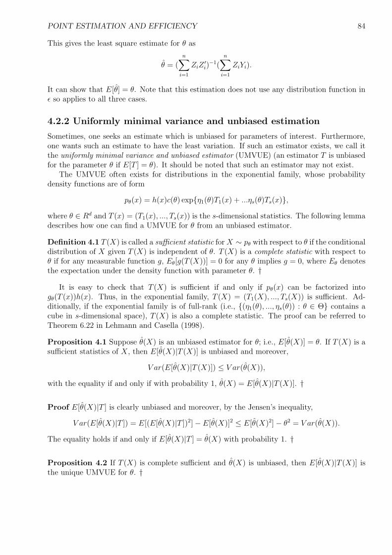
POINT ESTIMATION AND EFFICIENCY 84
This gives the least square estimate for θ as
θ = (n∑
i=1
ZiZ′i)−1(
n∑i=1
ZiYi).
It can show that E[θ] = θ. Note that this estimation does not use any distribution function inε so applies to all three cases.
4.2.2 Uniformly minimal variance and unbiased estimation
Sometimes, one seeks an estimate which is unbiased for parameters of interest. Furthermore,one wants such an estimate to have the least variation. If such an estimator exists, we call itthe uniformly minimal variance and unbiased estimator (UMVUE) (an estimator T is unbiasedfor the parameter θ if E[T ] = θ). It should be noted that such an estimator may not exist.
The UMVUE often exists for distributions in the exponential family, whose probabilitydensity functions are of form
pθ(x) = h(x)c(θ) expη1(θ)T1(x) + ...ηs(θ)Ts(x),where θ ∈ Rd and T (x) = (T1(x), ..., Ts(x)) is the s-dimensional statistics. The following lemmadescribes how one can find a UMVUE for θ from an unbiased estimator.
Definition 4.1 T (X) is called a sufficient statistic for X ∼ pθ with respect to θ if the conditionaldistribution of X given T (X) is independent of θ. T (X) is a complete statistic with respect toθ if for any measurable function g, Eθ[g(T (X))] = 0 for any θ implies g = 0, where Eθ denotesthe expectation under the density function with parameter θ. †
It is easy to check that T (X) is sufficient if and only if pθ(x) can be factorized intogθ(T (x))h(x). Thus, in the exponential family, T (X) = (T1(X), ..., Ts(X)) is sufficient. Ad-ditionally, if the exponential family is of full-rank (i.e., (η1(θ), ..., ηs(θ)) : θ ∈ Θ contains acube in s-dimensional space), T (X) is also a complete statistic. The proof can be referred toTheorem 6.22 in Lehmann and Casella (1998).
Proposition 4.1 Suppose θ(X) is an unbiased estimator for θ; i.e., E[θ(X)] = θ. If T (X) is asufficient statistics of X, then E[θ(X)|T (X)] is unbiased and moreover,
V ar(E[θ(X)|T (X)]) ≤ V ar(θ(X)),
with the equality if and only if with probability 1, θ(X) = E[θ(X)|T (X)]. †
Proof E[θ(X)|T ] is clearly unbiased and moreover, by the Jensen’s inequality,
V ar(E[θ(X)|T ]) = E[(E[θ(X)|T ])2]− E[θ(X)]2 ≤ E[θ(X)2]− θ2 = V ar(θ(X)).
The equality holds if and only if E[θ(X)|T ] = θ(X) with probability 1. †
Proposition 4.2 If T (X) is complete sufficient and θ(X) is unbiased, then E[θ(X)|T (X)] isthe unique UMVUE for θ. †
POINT ESTIMATION AND EFFICIENCY 85
Proof For any unbiased estimator for θ, denoted by T (X), we obtain from Proposition 4.1 thatE[T (X)|T (X)] is unbiased and
V ar(E[T (X)|T (X)]) ≤ V ar(T (X)).
Since E[E[T (X)|T (X)]− E[θ(X)|T (X)]] = 0 and E[T (X)|T (X)] and E[θ(X)|T (X)] are inde-pendent of θ, the completeness of T (X) gives that
E[T (X)|T (X)] = E[θ(X)|T (X)].
That is, V ar(E[θ(X)|T (X)]) ≤ V ar(T (X)). Thus, E[θ(X)|T (X)] is the UMVUE. The abovearguments also show that such a UMVUE is unique. †
Proposition 4.2 suggests two ways to derive the UMVUE in the presence of a completesufficient statistic T (X): one way is to find an unbiased estimator of θ then calculate theconditional expectation of this unbiased estimator given T (X); another way is to directly finda function g(T (X)) such that E[g(T (X))] = θ. The following example describes these twomethods.
Example 4.5 Suppose X1, ..., Xn are i.i.d according to the uniform distribution U(0, θ) and wewish to obtain a UMVUE of θ/2. From the joint density of X1, ..., Xn given by
1
θnI(X(n) < θ)I(X(1) > 0),
one can easily show X(n) is complete and sufficient for θ. Note E[X1] = θ/2. Thus, a UMVUEfor θ/2 is given by
E[X1|X(n)] =n + 1
n
X(n)
2.
The other way is to directly find a function g(X(n)) = θ/2 by noting
E[g(X(n))] =1
θn
∫ θ
0
g(x)nxn−1dx = θ/2.
Thus, we have ∫ θ
0
g(x)xn−1dx =θn+1
2n.
We differentiate both sides with respect to θ and obtain g(x) = n+1n
x2. Hence, we again obtain
the UMVUE for θ/2 is equal to (n + 1)X(n)/2n.Many more examples of the UMVUE can be found in Chapter 2 of Lehmann and Casella
(1998).
4.2.3 Robust estimation
In some regression problems, one may be concerned about outliers. For example, in a simplelinear regression, an extreme outlier may affect the fitted line greatly. One estimation approachcalled robust estimation approach is to propose an estimator which is little influenced by extreme

POINT ESTIMATION AND EFFICIENCY 86
observations. Often, for n i.i.d observations X1, ..., Xn, the robust estimation approach is tominimize an objective function with the form
∑ni=1 φ(Xi; θ).
Example 4.6 In linear regression, a model for (Y,X) is given by
Y = θ′X + ε,
where ε has mean zero. One robust estimator is to minimize
n∑i=1
|Yi − θ′Xi|
and the obtained estimator is called the least absolute deviation estimator. A more generalobjective function is to minimize
n∑i=1
φ(Yi − θ′Xi),
where φ(x) = |x|k, |x| ≤ C and φ(x) = Ck when |x| > C.
4.2.4 Estimating functions
In recent statistical inference, more and more estimators are based on estimating functions. Theuse of estimating functions has been extensively seen in semiparametric model. An estimatingfunction for θ is a measurable function f(X; θ) with E[f(X; θ)] = 0 or approximating zero.Then an estimator for θ using n i.i.d observations can be constructed by solving the estimatingequation
n∑i=1
f(Xi; θ) = 0.
The estimating function is useful, especially when there are other parameters in the model butonly θ is parameters of interest.
Example 4.7 We still consider the linear regression example. We can see that for any functionW (X), E[XW (X)(Y − θ′X)] = 0. Thus an estimating equation for θ can be constructed as
n∑i=1
XiW (Xi)(Yi − θ′Xi) = 0.
Example 4.8 Still in the regression example but we now assume the median of ε is zero. Itis easy to see that E[XW (X)sgn(Y − θ′X)] = 0. Then an estimating equation for θ can beconstructed as
n∑i=1
XiW (Xi)sgn(Yi − θ′Xi) = 0.
POINT ESTIMATION AND EFFICIENCY 87
4.2.5 Maximum likelihood estimation
The most commonly used method, at least in parametric models, is the maximum likelihoodestimation method: If n i.i.d observations X1, ..., Xn are generated from a distribution functionwith densities pθ(x), then it is reasonable to believe that the best value for θ should be the onemaximizing the observed likelihood function, which is defined as
Ln(θ) =n∏
i=1
pθ(Xi).
The obtained estimator θ is called the maximum likelihood estimator for θ. Many nice propertiesare possessed by the maximum likelihood estimators and we will particularly investigate thisissue in next chapter. Recent development has also seen the implementation of the maximumlikelihood estimation in semiparametric models and nonparametric models.
Example 4.9 Suppose X1, ..., Xn are i.i.d. observations from exp(θ). Then the likelihoodfunction for θ is equal to
Ln(θ) = θn exp−θ(X1 + ... + Xn).
The maximum likelihood estimator for θ is given by θ = Xn.
Example 4.10 The setting is Case B of Example 1.2. Suppose (Y1, Z1), ..., (Yn, Zn) are i.i.dwith the density function λ(y)eθ′z exp−Λ(y)eθ′zg(z), where g(z) is the known density functionof Z = z. Then the likelihood function for the parameters (θ, λ) is given by
Ln(θ, λ) =n∏
i=1
λ(Yi)e
θ′Zi exp−Λ(Yi)eθ′Zig(Zi)
.
It turns out that the maximum likelihood estimators for (θ, λ) do not exist. One way is to let Λbe a step function with jumps at Y1, ..., Yn and let λ(Yi) be the jump size, denoted as pi. Thenthe likelihood function becomes
Ln(θ, p1, ..., pn) =n∏
i=1
pie
θ′Zi exp−∑
Yj≤Yi
pjeθ′Zig(Zi)
.
The maximum likelihood estimators for (θ, p1, ..., pn) are given as: θ solves the equation
n∑i=1
Zi
[1−
∑Yj≥Yi
Zjeθ′Zj
∑Yj≥Yi
eθ′Zj
]= 0
and
pi =1∑
Yj≥Yieθ′Zj
.
POINT ESTIMATION AND EFFICIENCY 88
4.2.6 Bayesian estimation
In this estimation approach, the parameter θ in the model distributions pθ(x) is treated asa random variable with some prior distribution π(θ). The estimator for θ is defined as a valuedepending on the data and minimizing the expected loss function or the maximal loss function,where the loss function is denoted as l(θ, θ(X)). The usual loss function includes the quadraticloss (θ− θ(X))2, the absolute loss |θ− θ(X)| etc. It often turns out that θ(X) can be determinedfrom the posterior distribution of P (θ|X) = P (X|θ)P (θ)/P (X).
Example 4.11 Suppose X ∼ N(θ, 1), where θ has an improper prior distribution of beinguniform in (−∞,∞). It is clear that the estimator θ(X), minimizing the quadratic loss E[(θ−θ(X))2], is the posterior mean E[θ|X] = X.
4.2.7 Concluding remarks
We have reviewed a few methods which are seen in many statistical problems. However we havenot exhausted all estimation approaches. Other estimation methods include the conditionallikelihood estimation, the profile likelihood estimation, the partial likelihood estimation, theempirical Bayesian estimation, the minimax estimation, the rank estimation, L-estimation andetc.
With a number of estimators, one natural question is to decide which estimator is the bestchoice. The first criteria is that the estimator must be unbiased or at least consistent with thetrue parameter. Such a property is called the first order efficiency. In order to make a preciseestimation, we may also want the estimator to have as small variance as possible. The issuethen becomes the second order efficiency, which we will discuss in the next section.
4.3 Cramer-Rao Bounds for Parametric Models
4.3.1 Information bound in one-dimensional model
First, we assume the model is one-dimensional parametric model P = Pθ : θ ∈ Θ with Θ ⊂ R.We assume:A. X ∼ Pθ on (Ω,A) with θ ∈ Θ.B. pθ = dPθ/dµ exists where µ is a σ-finite dominating measure.C. T (X) ≡ T estimates q(θ) has Eθ[|T (X)|] < ∞; set b(θ) = Eθ[T ]− q(θ).D. q′(θ) ≡ q(θ) exists.
Theorem 4.1 (Information bound or Cramer-Rao Inequality) Suppose:(C1) Θ is an open subset of the real line.(C2) There exists a set B with µ(B) = 0 such that for x ∈ Bc, ∂pθ(x)/∂θ exists for all θ.Moreover, A = x : pθ(x) = 0 does not depend on θ.(C3) I(θ) = Eθ[lθ(X)2] > 0 where lθ(x) = ∂ log pθ(x)/∂θ. Here, I(θ) is the called the Fisherinformation for θ and lθ is called the score function for θ.(C4)
∫pθ(x)dµ(x) and
∫T (x)pθ(x)dµ(x) can both be differentiated with respect to θ under the
integral sign.
POINT ESTIMATION AND EFFICIENCY 89
(C5)∫
pθ(x)dµ(x) can be differentiated twice under the integral sign.If (C1)-(C4) hold, then
V arθ(T (X)) ≥ q(θ) + b(θ)2
I(θ),
and the lower bound is equal to q(θ)2/I(θ) if T is unbiased. Equality holds for all θ if and onlyif for some function A(θ), we have
lθ(x) = A(θ)T (x)− Eθ[T (X)], a.e.µ.
If, in addition, (C5) holds, then
I(θ) = −Eθ
∂2
∂θ2log pθ(X)
= −Eθ[lθ(X)].
†
Proof Note
q(θ) + b(θ) =
∫T (x)pθ(x)dµ(x) =
∫
Ac∩Bc
T (x)pθ(x)dµ(x).
Thus from (C2) can (C4),
q(θ) + b(θ) =
∫
Ac∩Bc
T (x)lθ(x)pθ(x)dµ(x) = Eθ[T (X)lθ(X)].
On the other hand, since∫
Ac∩Bc pθ(x)dµ(x) = 1,
0 =
∫
Ac∩Bc
lθ(x)pθ(x)dµ(x) = Eθ[lθ(X)].
Thenq(θ) + b(θ) = Cov(T (X), lθ(X)).
By the Cauchy-Schwartz inequality, we obtain
|q(θ) + b(θ)| ≤ V ar(T (X))V ar(lθ(X)).
The equality holds if and only if
lθ(X) = A(θ) T (X)− Eθ[T (X)] , a.s.
Finally, if (C5) holds, we further differentiate
0 =
∫lθ(x)pθ(x)dµ(x)
and obtain
0 =
∫lθ(x)pθ(x)dµ(x) +
∫lθ(x)2pθ(x)dµ(x).
Thus, we obtain the equality I(θ) = −Eθ[lθ(X)]. †
POINT ESTIMATION AND EFFICIENCY 90
Theorem 4.1 implies that the variance of any unbiased estimator has a lower bound q(θ)2/I(θ),which is intrinsic to the parametric model. Especially, if q(θ) = θ, then the lower bound for thevariance of unbiased estimator for θ is the inverse of the information. The following examplescalculate this bound for some parametric models.
Example 4.12 Suppose X1, ..., Xn are i.i.d Poisson(θ). The density function for (X1, ..., Xn)is given by
pθ(X1, ..., Xn) = −nθ + nXn log θ −n∑
i=1
log(Xi!).
Thus,
lθ(X1, ..., Xn) =n
θ(Xn − θ).
It is direct to check all the regularity conditions of Theorem 3.1 are satisfied. Then In(θ) =n2/θ2V ar(Xn) = n/θ. The Carmer-Rao bound for θ is equal to θ/n. On the other hand, wenote Xn is an unbiased estimator of θ. Moreover, since Xn is the complete statistic for θ. Xn
is indeed the UMVUE of θ. Note V ar(Xn) = θ/n. We conclude that Xn attains the lowerbound. However, although Tn = X2
n − n−1Xn is unbiased for θ2 and it is UMVUE of θ2, wefind V ar(Tn) = 4θ3/n + 2θ2/n2 > the Cramer-Rao lower bound for θ2. In other words, someUMVUE attains the lower bound but some do not.
Example 4.13 Suppose X1, ..., Xn are i.i.d with density pθ(x) = g(x − θ) where g is knowndensity. This family is the one-dimensional location model. Assume g′ exists and the regularityconditions in Theorem 4.1 are satisfied. Then
In(θ) = nEθ[g′(X − θ)
g(X − θ)
2
] = n
∫g′(x)2
g(x)dx.
Note the information does not depend on θ.
Example 4.14 Suppose X1, ..., Xn are i.i.d with density pθ(x) = g(x/θ)/θ where g is a knowndensity function. This model is one-dimensional scale model with the common shape g. It isdirect to calculate
In(θ) =n
θ2
∫(1 + y
g′(y)
g(y))2g(y)dy.
4.3.2 Information bound in multi-dimensional model
We can extend Theorem 4.1 to the case in which the model is k-dimensional parametric family:P = Pθ : θ ∈ Θ ⊂ Rk. Similar to Assumptions A-C, we assume Pθ has density functionpθ with respect to some σ-finite dominating measure µ; T (X) is an estimator for q(θ) withEθ[|T (X)|] < ∞ and b(θ) = Eθ[T (X)]− q(θ is the bias of T (X); q(θ) = ∇q(θ) exists.
Theorem 4.2 (Information inequality) Suppose that(M1) Θ an open subset in Rk.(M2) There exists a set B with µ(B) = 0 such that for x ∈ Bc, ∂pθ(x)/∂θi exists for all θ and
POINT ESTIMATION AND EFFICIENCY 91
i = 1, ..., k. The set A = x : pθ(x) = 0 does no depend on θ.(M3) The k × k matrix I(θ) = (Iij(θ)) = Eθ[lθ(X)lθ(X)′] > 0 is a positive definite where
lθi(x) =
∂
∂θi
log pθ(x).
Here, I(θ) is called the Fisher information matrix for θ and lθ is called the score for θ.(M4)
∫pθ(x)dµ(x) and
∫T (x)pθ(x)dµ(x) can both be differentiated with respect to θ under
the integral sign.(M5)
∫pθ(x)dµ(x) can be differentiated twice with respect to θ under the integral sign.
If (M1)-(M4) holds, than
V arθ(T (X)) ≥ (q(θ) + b(θ))′I−1(θ)(q(θ) + b(θ))
and this lower bound is equal q(θ)′I(θ)−1q(θ) if T (X) is unbiased. If, in addition, (M5) holds,then
I(θ) = −Eθ[lθθ(X)] = −(Eθ
∂2
∂θi∂θj
log pθ(X)
).
†
Proof Under (M1)-(M4), we have
q(θ) + b(θ) =
∫T (x)lθ(x)pθ(x)dµ(x) = Eθ[T (x)lθ(X)].
On the other hand, from∫
pθ(x)dµ(x) = 1, 0 = Eθ[lθ(X)]. Thus,
|
q(θ) + b(θ)′
I(θ)−1
q(θ) + b(θ)|
= |Eθ[T (X)(q(θ) + b(θ))′I(θ)−1lθ(X)]|= |Covθ(T (X), (q(θ) + b(θ))′I(θ)−1lθ(X))|≤
√V arθ(T (X))(q(θ) + b(θ))′I(θ)−1(q(θ) + b(θ)).
We obtain the information inequality. In addition, if (M5) holds, we further differentiate∫lθ(x)pθ(x)dµ(x) = 0 and obtain the then
I(θ) = −Eθ[lθθ(X)] = −(Eθ
∂2
∂θi∂θj
log pθ(X)
).
†
Example 4.15 The Weibull family P is the parametric model with densities
pθ(x) =β
α(x
α)β−1 exp
−(
x
α)β
I(x ≥ 0)
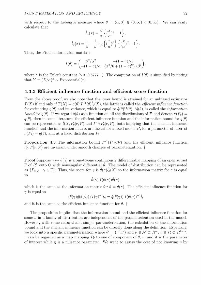
POINT ESTIMATION AND EFFICIENCY 92
with respect to the Lebesgue measure where θ = (α, β) ∈ (0,∞) × (0,∞). We can easilycalculate that
lα(x) =β
α
(x
α)β − 1
,
lβ(x) =1
β− 1
βlog
(x
α)β
(x
α)β − 1
.
Thus, the Fisher information matrix is
I(θ) =
(β2/α2 −(1− γ)/α
−(1− γ)/α π2/6 + (1− γ)2 /β2
),
where γ is the Euler’s constant (γ ≈ 0.5777...). The computation of I(θ) is simplified by notingthat Y ≡ (X/α)β ∼ Exponential(x).
4.3.3 Efficient influence function and efficient score function
From the above proof, we also note that the lower bound is attained for an unbiased estimatorT (X) if and only if T (X) = q(θ)′I−1(θ)lθ(X), the latter is called the efficient influence functionfor estimating q(θ) and its variance, which is equal to q(θ)′I(θ)−1q(θ), is called the informationbound for q(θ). If we regard q(θ) as a function on all the distributions of P and denote ν(Pθ) =q(θ), then in some literature, the efficient influence function and the information bound for q(θ)can be represented as l(X,Pθ|ν,P) and I−1(Pθ|ν,P), both implying that the efficient influencefunction and the information matrix are meant for a fixed model P , for a parameter of interestν(Pθ) = q(θ), and at a fixed distribution Pθ.
Proposition 4.3 The information bound I−1(P |ν,P) and the efficient influence functionl(·, P |ν,P) are invariant under smooth changes of parameterization. †
Proof Suppose γ 7→ θ(γ) is a one-to-one continuously differentiable mapping of an open subsetΓ of Rk onto Θ with nonsingular differential θ. The model of distribution can be representedas Pθ(γ) : γ ∈ Γ. Thus, the score for γ is θ(γ)lθ(X) so the information matrix for γ is equalto
θ(γ)′I(θ(γ))θ(γ),
which is the same as the information matrix for θ = θ(γ). The efficient influence function forγ is equal to
(θ(γ)q(θ(γ)))′I(γ)−1lγ = q(θ(γ))′I(θ(γ))−1lθ
and it is the same as the efficient influence function for θ. †
The proposition implies that the information bound and the efficient influence function forsome ν in a family of distribution are independent of the parameterization used in the model.However, with some natural and simple parameterization, the calculation of the informationbound and the efficient influence function can be directly done along the definition. Especially,we look into a specific parameterization where θ′ = (ν ′, η′) and ν ∈ N ⊂ Rm, η ∈ H ⊂ Rk−m.ν can be regarded as a map mapping Pθ to one of component of θ, ν, and it is the parameterof interest while η is a nuisance parameter. We want to assess the cost of not knowing η by
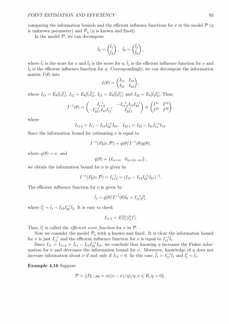
POINT ESTIMATION AND EFFICIENCY 93
comparing the information bounds and the efficient influence functions for ν in the model P (ηis unknown parameter) and Pη (η is known and fixed).
In the model P , we can decompose
lθ =
(l1l2
), lθ =
(l1l2
),
where l1 is the score for ν and l2 is the score for η, l1 is the efficient influence function for ν andl2 is the efficient influence function for η. Correspondingly, we can decompose the informationmatrix I(θ) into
I(θ) =
(I11 I12
I21 I22
),
where I11 = Eθ[l1l′1], I12 = Eθ[l1l
′2], I21 = Eθ[l2l
′1], and I22 = Eθ[l2l
′2]. Thus,
I−1(θ) =
(I−111·2 −I−1
11·2I12I−122
−I−122·1I21I
−111 I−1
22·1
)≡
(I11 I12
I21 I22
),
whereI11·2 = I11 − I12I
−122 I21, I22·1 = I22 − I21I
−111 I12.
Since the information bound for estimating ν is equal to
I−1(Pθ|ν,P) = q(θ)′I−1(θ)q(θ),
where q(θ) = ν, andq(θ) =
(Im×m 0m×(k−m)
),
we obtain the information bound for ν is given by
I−1(Pθ|ν,P) = I−111·2 = (I11 − I12I
−122 I21)
−1.
The efficient influence function for ν is given by
l1 = q(θ)′I−1(θ)lθ = I−111·2l
∗1,
where l∗1 = l1 − I12I−122 l2. It is easy to check
I11·2 = E[l∗1(l∗1)′].
Thus, l∗1 is called the efficient score function for ν in P .Now we consider the model Pη with η known and fixed. It is clear the information bound
for ν is just I−111 and the efficient influence function for ν is equal to I−1
11 l1.Since I11 > I11·2 = I11 − I12I
−122 I21, we conclude that knowing η increases the Fisher infor-
mation for ν and decreases the information bound for ν. Moreover, knowledge of η does notincrease information about ν if and only if I12 = 0. In this case, l1 = I−1
11 l1 and l∗1 = l1.
Example 4.16 Suppose
P = Pθ : pθ = φ((x− ν)/η)/η, ν ∈ R, η > 0 .
POINT ESTIMATION AND EFFICIENCY 94
Note that
lν(x) =x− ν
η2, lη(x) =
1
η
(x− ν)2
η2− 1
.
Then the information matrix I(θ) is given by by
I(θ) =
(η−2 00 2η−2
).
Then we can estimate the ν equally well whether we know the variance or not.
Example 4.17 If we reparameterize the above model as
Pθ = N(ν, η2 − ν2), η2 > ν2.
The easy calculation shows that I12(θ) = νη/(η2 − ν2)2. Thus lack of knowledge of η in thisparameterization does change the information bound for estimation of ν.
We provide a nice geometric way of calculating the efficient score function and the efficientinfluence function for ν. For any θ, the linear space L2(Pθ) = g(X) : Eθ[g(X)2] < ∞ is aHilbert space with the inner product defined as
< g1, g2 >= E[g1(X)g2(X)].
On this Hilbert space, we can define the concept of the projection. For any closed linear spaceS ⊂ L2(Pθ) and any g ∈ L2(Pθ), the projection of g on S is g ∈ S such that g− g is orthogonalto any g∗ in S in the sense that
E[(g(X)− g(X))g∗(X)] = 0, ∀g∗ ∈ S.
The orthocomplement of S is a linear space with all the g ∈ L2(P ) such that g is orthogonalto any g∗ ∈ S. The above concepts agree with the usual definition in the Euclidean space.The following theorem describes the calculation of the efficient score function and the efficientinfluence function.
Theorem 4.3 A. The efficient score function l∗1(·, Pθ|ν,P) is the projection of the score functionl1 on the orthocomplement of [l2] in L2(Pθ), where [l2] is the linear span of the components ofl2.B. The efficient influence function l(·, Pθ|ν,Pη) is the projection of the efficient influence functionl1 on [l1] in L2(Pθ). †
Proof A. Suppose the projection of l1 on [l2] is equal to Σl2 for some matrix Σ. Since E[(l1 −Σl2)l
′2] = 0, we obtain Σ = I12I
−122 then the projection on the orthocomplement of [l2] is equal
to l1 − I12I−122 l2, which is the same as l∗1.
B. After the algebra, we note
l1 = I−111·2(l1 − I12I
−122 l2) = (I−1
11 + I−111 I12I
−122·1I21I
−111 )(l1 − I12I
−122 l2) = I−1
11 l1 − I−111 I12l2.
Since from A, l2 is orthogonal to l1, the projection of l1 on [l1] is equal I−111 l1, which is the
efficient influence function l(·, Pθ|ν,Pη). †
POINT ESTIMATION AND EFFICIENCY 95
The following table describes the relationship among all these terminologies.Term Notation P (η unknown) Pη (η known)
efficient score l∗1(, P |ν, ·) l∗1 = l1 − I12I−122 l2 l1
information I(P |ν, ·) E[l∗1(l∗1)′] = I11 − I12I
−122 I22 I11
efficient l1(·, P |ν, ·) l1 = I11l1 + I12l2 = I−111·2l
∗1 I−1
11 l1influence information = I−1
11 l1 − I−111 I12l2
information bound I−1(P |ν, ·) I11 = I−111·2 = I−1
11 + I−111 I12I
−122·1I21I
−111 I−1
11
4.4 Asymptotic Efficiency Bound
4.4.1 Regularity conditions and asymptotic efficiency theorems
The Cramer-Rao bound can be considered as the lower bound for any unbiased estimator infinite sample. One may ask whether such a bound still holds in large sample. To be specific,we suppose X1, ..., Xn are i.i.d Pθ (θ ∈ R) and an estimator Tn for θ satisfies that
√n(Tn − θ) →d N(0, V (θ)2).
Then the question is whether V (θ)2 ≥ 1/I(θ). Unfortunately, this may not be true as thefollowing example due to Hodges gives one counterexample.
Example 4.18 Let X1, ..., Xn be i.i.d N(θ, 1) so that I(θ) = 1. Let |a| < 1 and define
Tn =
Xn if|Xn| > n−1/4
aXn if|Xn| ≤ n−1/4.
Then
√n(Tn − θ) =
√n(Xn − θ)I(|Xn| > n−1/4) +
√n(aXn − θ)I(|Xn| ≤ n−1/4)
=d ZI(|Z +√
nθ| > n1/4) +aZ +
√n(a− 1)θ
I(|Z +
√nθ| ≤ n1/4)
→a.s. ZI(θ 6= 0) + aZI(θ = 0).
Thus, the asymptotic variance of√
nTn is equal 1 for θ 6= 0 and a2 for θ = 0. The latter issmaller than the Cramer-Rao bound. In other words, Tn is a superefficient estimator.
To avoid the Hodge’s superefficient estimator, we need impose some conditions to Tn inaddition to the weak convergence of
√n(Tn − θ). One such condition is called locally regular
condition in the following sense.
Definition 4.2 Tn is a locally regular estimator of θ at θ = θ0 if, for every sequence θn ⊂ Θwith
√n(θn − θ) → t ∈ Rk, under Pθn ,
(local regularity)√
n(Tn − θn) →d Z, as n →∞
where the distribution of Z depend on θ0 but not on t. Thus the limit distribution of√
n(Tn−θn)does not depend on the direction of approach t of θn to θ0. Tn is a locally Gaussian regularif Z has normal distribution. †

POINT ESTIMATION AND EFFICIENCY 96
In the above definition,√
n(Tn − θn) →d Z under Pθn is equivalent to saying that for anybounded and continuous function g, Eθn [g(
√n(Tn−θn))] → E[g(Z)]. One can consider a locally
regular estimator as the one whose limit distribution is locally stable: if data are generated undera model not far from a given model, the limit distribution of centralized estimator remains thesame.
Furthermore, the locally regular condition, combining with the following two additionalconditions, gives the results that the Cramer-Rao bound is also the asymptotic lower bound:
(C1) (Hellinger differentiability) A model P = Pθ : θ ∈ Rk is a parametric model dominatedby a σ-finite measure µ. It is called a Hellinger-differentiable parametric model if
‖√pθ+h −√pθ − 1
2h′lθ
√pθ‖L2(µ) = o(|h|),
where pθ = dPθ/dµ.
(C2) (Local Asymptotic Normality (LAN)) In a model P = Pθ : θ ∈ Rk dominated by aσ-finite measure µ, suppose pθ = dPθ/dµ. Let l(x; θ) = log p(x, θ) and let
ln(θ) =n∑
i=1
l(Xi; θ)
be the log-likelihood function of X1, ..., Xn. The local asymptotic normality condition at θ0 is
ln(θ0 + n−1/2t)− ln(θ0) →d N(−1
2t′I(θ0)t, t
′I(θ0)t)
under Pθ0 .Both conditions (C1) and (C2) are the smooth conditions imposed on the parametric models.
In other words, we do not allow a model whose parameterization is irregular. An irregular modelis seldom encountered in practical use.
The following theorem gives the main results.
Theorem 4.4 (Hajek’s convolution theorem) Under conditions (C1)-(C2) with I(θ0) non-singular. For any locally regular estimator of θ, Tn, the limit distribution of
√n(Tn − θ0)
under Pθ0 satisfiesZ =d Z0 + ∆0,
where Z0 ∼ N(0, I−1(θ0)) is independent of ∆0. †
As a corollary, if V (θ0)2 is the asymptotic variance of
√n(Tn − θ0), then V (θ0)
2 ≥ I−1(θ0).Thus, the Cramer-Rao bound is a lower bound for the asymptotic variances of any locallyregular estimators. Furthermore, we obtain the following corollary from Theorem 4.4.
Corollary 4.1 Suppose that Tn is a locally regular estimator of θ at θ0 and that U : Rk → R+
is bowl-shaped loss function; i.e., U(x) = U(−x) and x : U(x) ≤ c is convex for any c ≥ 0.Then
lim infn
Eθ0 [U(√
n(Tn − θ0))] ≥ E[U(Z0)],
where Z0 ∼ N(0, I(θ0)−1). †
POINT ESTIMATION AND EFFICIENCY 97
Corollary 4.2 (Hajek-Le Cam asymptotic minmax theorem) Suppose that (C2) holds,that Tn is any estimator of θ, and U is bowl-shaped. Than
limδ→0
lim infn
supθ:√
n|θ−θ0|≤δ
Eθ[U(√
n(Tn − θ))] ≥ E[U(Z0)],
where Z0 ∼ N(0, I(θ0)−1). †
In summary, the two corollaries conclude that the asymptotic loss of any regular estimatorsis at least the loss given by the distribution Z0. Thus, from this point of view, Z0 is also thedistribution of most efficiency. The proofs of the two corollaries are beyond this book so areskipped.
4.4.2 Le Cam’s lemmas
Before proving Theorem 4.4, we introduce the contiguity definition and the Le Cam’s lemmas.Consider a sequence of measure spaces (Ωn,An, µn) and on each measure space, we have twoprobability measure Pn and Qn with Pn ≺≺ µn and Qn ≺≺ µn. Let pn = dPn/dµn andqn = dQn/dµn be the corresponding densities of Pn and Qn. We define the likelihood ratios
Ln =
qn/pn if pn > 01 if qn = pn = 0n if qn > 0 = pn.
Definition 4.3 (Contiguity) The sequence Qn is contiguous to Pn if for every sequenceBn ∈ An for which Pn(Bn) → 0 it follows that Qn(Bn) → 0. †
Thus contiguity of Qn to Pn means that Qn is “asymptotically absolutely continuous”with respect to Pn. We denote Qn / Pn. Two sequences are contiguous to each other ifQn / Pn and Pn / Qn and we write Pn / .Qn.
Definition 4.4 (Asymptotic orthogonality) The sequence Qn is asymptotically orthogonal toPn if there exists a sequence Bn ∈ An such that Qn(Bn) → 1 and Pn(Bn) → 0. †
Proposition 4.4 (Le Cam’s first lemma) Suppose under Pn, Ln →d L with E[L] = 1. ThenQn / Pn. On the contrary, if Qn / Pn and under Pn, Ln →d L, then E[L] = 1. †
Proof We fist prove the first half of the lemma. Let Bn ∈ An with Pn(Bn) → 0. ThenIΩn−Bn converges to 1 in probability under Pn. Since Ln is asymptotically tight, (Ln, IΩn−Bn) isasymptotically tight under Pn. Thus, by the Helly’s lemma, for every subsequence of n, thereexists a further subsequence such that (Ln, IΩn−Bn) →d (L, 1). By the Protmanteau Lemma,since (v, t) 7→ vt is continuous and nonnegative,
lim infn
Qn(Ωn −Bn) ≥ lim infn
∫IΩn−Bn
dQn
dPn
dPn ≥ E[L] = 1.
We obtain Qn(Bn) → 0. Thus Qn / Pn.

POINT ESTIMATION AND EFFICIENCY 98
We then prove the second half of the lemma. The probability measure Rn = (Pn + Qn)/2dominate both Pn and Qn. Note that dPn/dQn, Ln and Wn = dPn/dRn are tight withrespect to Qn, Pn and Rn. By the Prohov’s theorem, for any subsequence, there existsa further subsequence such that
dPn
dQn
→d U, under Qn,
Ln =dQn
dPn
→d L, under Pn,
Wn =dPn
dRn
→d W, under Rn
for certain random variables U , V , and W . Since ERn [Wn] = 1 and 0 ≤ Wn ≤ 2, we obtainE[W ] = 1. For a given bounded, continuous function f , define g(ω) = f(ω/(2− ω))(2− ω) for0 ≤ ω < 2 and g(2) = 0. Then g is continuous. Thus,
EQn [f(dPn
dQn
)] = ERn [f(dPn
dQn
)dQn
dRn
] = ERn [g(Wn)] → E[f(W
2−W)(2−W )].
Since EQn [f(dPn/dQn)] → E[f(U)], we have
E[f(U)] = E[f(W
2−W)(2−W )].
Choose fm in the above expression such that fm ≤ 1 and fm decreases to I0. From thedominated convergence theorem, we have
P (U = 0) = E[I0(W
2−W)(2−W )] = 2P (W = 0).
However, since
Pn( dPn
dQn
≤ εn ∩ qn > 0) ≤∫
dPn/dQn≤εn
dPn
dQn
dQn ≤ εn → 0
and Qn / Pn,
P (U = 0) = limn
P (U ≤ εn) ≤ lim infn
Qn(dPn
dQn
≤ εn) = lim infn
Qn( dPn
dQn
≤ εn ∩ qn > 0) = 0.
That is, P (W = 0) = 0. Similar to the above deduction, we obtain that
E[f(L)] = E[f(2−W
W)W ].
Choose fm in the expression such that fm(x) increase to x. By the monotone convergencetheorem, we have
E[L] = E[(2−W )I(W > 0)] = 2P (W > 0)− 1 = 1.
†
POINT ESTIMATION AND EFFICIENCY 99
As a corollary, we have
Corollary 4.3 If log Ln →d N(−σ2/2, σ2) under Pn, then Qn / Pn. †
Proof Under Pn, Ln →d exp−σ2/2+σZ where the limit has mean 1. The result thus followsfrom Proposition 4.4. †
Proposition 4.5 (Le Cam’s third lemma) Let Pn and Qn be sequence of probability mea-sures on measurable spaces (Ωn,An), and let Xn : Ωn → Rk be a sequence of random vectors.Suppose that Qn / Pn and under Pn,
(Xn, Ln) →d (X, L).
Then G(B) = E[IB(X)L] defines a probability measure, and under Qn, Xn →d G. †
Proof Because V ≥ 0, for countable disjoint sets B1, B2, ..., by the monotone convergencetheorem,
G(∪Bi) = E[limn
(IB1 + ... + IBn)L] = limn
n∑i=1
E[IBiL] =
∞∑i=1
G(Bi).
From Proposition 4.4, E[L] = 1. Then G(Ω) = 1. G is a probability measure. Moreover, forany measurable simple function f , it is easy to see
∫fdG = E[f(X)L].
Thus, this equality holds for any measurable function f . In particular, for continuous andnonnegative function f , (x, v) 7→ f(x)v is continuous and nonnegative. Thus,
lim inf EQn [f(Xn)] ≥ lim inf
∫f(Xn)
dQn
dPn
dPn ≥ E[f(X)L].
Thus, under Qn, Xn →d G. †
Remark 4.1 In fact, the name Le Cam’s third lemma is often reserved for the following result.If under Pn,
(Xn, log Ln) →d Nk+1
( (µ
−σ2/2
),
(Σ ττ σ2
) ),
then under Qn, Xn →d Nk(µ + τ, Σ). This result follows from Proposition 4.5 by noticing thatthe characteristic function of the limit distribution G is equal to E[eitXeY ], where (X, Y ) hasthe joint distribution
Nk+1
( (µ
−σ2/2
),
(Σ ττ σ2
) ).
Such a characteristic function is equal expit′(µ + τ) − t′Σt/2, which is the characteristicfunction for Nk(µ + τ, Σ).
POINT ESTIMATION AND EFFICIENCY 100
4.4.3 Proof of the convolution theorem
Equipped with the Le Cam’s two lemmas, we start to prove the convolution result in Theorem4.4.
Proof of Theorem 4.4 We divide the proof into the following steps.Step I. We first prove that the Hellinger differentiability condition (C1) implies that Pθ0 [lθ0 ] = 0,the Fisher information I(θ0) = Eθ0 [lθ0l
′θ0
] exists, and moreover, for every convergent sequencehn → h, as n →∞,
logn∏
i=1
pθ0+hn/√
n
pθ0
(Xi) =1√n
n∑i=1
h′lθ0(Xi)− 1
2h′Iθ0h + rn,
where rn →p 0. To see that , we abbreviate pn, p, g as pθ0+h/√
n, pθ0 , h′lθ0 . Since√
n(√
pn−√p)converges in L2(µ) to g
√p/2,
√pn converges to
√p in L2(µ). Then
E[g] =
∫1
2g√
p2√
pdµ = limn→∞
∫ √n(√
pn −√p)(√
pn +√
p)dµ = 0.
Thus, Eθ0 [lθ0 ] = 0. Let Wni = 2(√
pn(Xi)/p(Xi)− 1). We have
V ar(n∑
i=1
Wni − 1√n
n∑i=1
g(Xi)) ≤ E[(√
nWni − g(Xi))2] → 0,
E[n∑
i=1
Wni] = 2n(
∫ √pn√
pdµ− 1) = −n
∫[√
pn −√p]2dµ → −1
4E[g2].
Here, E[g2] = h′I(θ0)h. By the Chebyshev’s inequality, we obtain
n∑i=1
Wni =1√n
n∑i=1
g(Xi)− 1
4E[g2] + an,
where an →p 0.Next, by the Taylor expansion,
logn∏
i=1
pn
p(Xi) = 2
n∑i=1
log(1 +1
2Wni) =
n∑i=1
Wni − 1
4
n∑i=1
W 2ni +
1
2
n∑i=1
W 2niR(Wni),
where R(x) → 0 as x → 0. Since E[(√
nWni − g(Xi))2] → 0, nW 2
ni = g(Xi)2 + Ani where
E[|Ani|] → 0. Then∑n
i=1 W 2ni →p E[g2]. Moreover,
nP (|Wni| > ε√
2) ≤ nP (g(Xi)2 > nε2)+nP (|Ani| > nε2) ≤ ε−2E[g2I(g2 > nε2)]+ε−2E[|Ani|] → 0.
The left-hand side is the upper bound for P (max1≤i≤n |Wni| > ε). Thus, max1≤i≤n |Wni| con-verges to zero in probability; so is max1≤i≤n |R(Wni)|. Therefore,
logn∏
i=1
pn
p(Xi) =
n∑i=1
Wni − 1
4E[g2] + bn,
POINT ESTIMATION AND EFFICIENCY 101
where bn →p 0. Combining all the results, we obtain
logn∏
i=1
pθ0+hn/√
n
pθ0
(Xi) =1√n
n∑i=1
h′lθ0(Xi)− 1
2h′Iθ0h + rn,
where rn →pn 0.
Step II. Let Qn be the probability measure with density∏n
i=1 pθ0+h/√
n(xi) and Pn be theprobability measure with
∏ni=1 pθ0(xi). Define
Sn =√
n(Tn − θ0), ∆n =1√n
n∑i=1
lθ0(Xi).
By the assumptions, Sn weakly converges to some distribution and so is ∆n under Pn; thus,(Sn, ∆n) is tight under Pn. By the Prohorov’s theorem, for any subsequence, there exists afurther subsequence such that (Sn, ∆n) →d (S, ∆) under Pn. From Step I, we immediatelyobtain that under Pn,
(Sn, logdQn
dPn
) →d (S, h′∆− 1
2h′I(θ0)h).
Since under Pn, dQn/dPn weakly converges to N(−h′I(θ0)h/2, h′I(θ0)h), Corollary 4.3 givesthat Qn/Pn. Then from the Le Cam’s third lemma, under Qn, Sn =
√n(Tn−θ0) converges
in distribution to a distribution Gh. Clearly, Gh is the same as distribution with Z + h.
Step III. We show Z = Z0 + ∆0 where Z0 ∼ N(0, I(θ0)−1) is independent of ∆0. From Step II,
we haveEθ0+h/
√n[expit′Sn] → expit′hE[expit′Z].
On the other hand,
Eθ0+h/√
n[expit′Sn] = Eθ0 [expit′Sn + logdQn
dPn
] + o(1) → Eθ0 [expit′Z + h′∆− 1
2h′I(θ0)h].
We have
Eθ0 [expit′Z + h′∆− 1
2h′I(θ0)h] = expit′hEθ0 [expit′Z]
and it should hold for any complex number t and h. We let h = −i(t′ − s′)I(θ0)−1 and obtain
Eθ0 [expit′(Z − I(θ0)−1∆) + is′I(θ0)
−1∆] = Eθ0 [expit′Z +1
2t′I(θ0)
−1t] exp−1
2s′I(θ0)
−1s.This implies that ∆0 = (Z − I(θ0)
−1∆) is independent of Z0 = I(θ0)−1∆ and Z0 has the
characteristics function exp−s′I(θ0)−1s/2, meaning Z0 ∼ N(0, I(θ0)
−1). Then Z = Z0 + ∆0.†
The convolution theorem indicates that if Tn is locally regular and the model P is theHellinger differentiable and LAN, then the Cramer-Rao bound is also the asymptotic lowerbound. We have shown that the result holds for estimating θ. In fact, the same procedureapplies to estimating q(θ) where q is differentiable at θ0. Then the local regularity condition isthat under Pθ0+h/
√n, √
n(Tn − q(θ0 + h/√
n)) →d Z,
where Z is independent of h. The result in Theorem 4.4 then becomes that Z = Z0 +∆0 whereZ0 ∼ N(0, q(θ0)
′I(θ0)−1q(θ0)) is independent of ∆0.
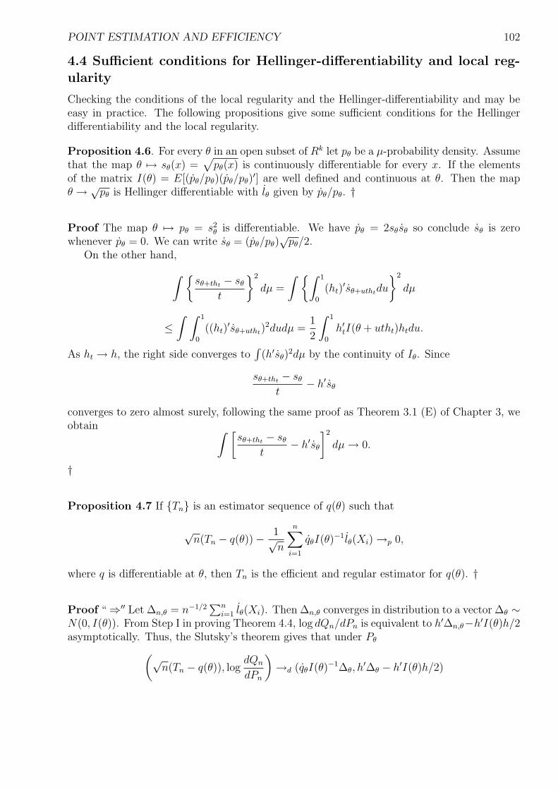
POINT ESTIMATION AND EFFICIENCY 102
4.4 Sufficient conditions for Hellinger-differentiability and local reg-ularity
Checking the conditions of the local regularity and the Hellinger-differentiability and may beeasy in practice. The following propositions give some sufficient conditions for the Hellingerdifferentiability and the local regularity.
Proposition 4.6. For every θ in an open subset of Rk let pθ be a µ-probability density. Assumethat the map θ 7→ sθ(x) =
√pθ(x) is continuously differentiable for every x. If the elements
of the matrix I(θ) = E[(pθ/pθ)(pθ/pθ)′] are well defined and continuous at θ. Then the map
θ → √pθ is Hellinger differentiable with lθ given by pθ/pθ. †
Proof The map θ 7→ pθ = s2θ is differentiable. We have pθ = 2sθsθ so conclude sθ is zero
whenever pθ = 0. We can write sθ = (pθ/pθ)√
pθ/2.On the other hand,
∫ sθ+tht − sθ
t
2
dµ =
∫ ∫ 1
0
(ht)′sθ+uthtdu
2
dµ
≤∫ ∫ 1
0
((ht)′sθ+utht)
2dudµ =1
2
∫ 1
0
h′tI(θ + utht)htdu.
As ht → h, the right side converges to∫
(h′sθ)2dµ by the continuity of Iθ. Since
sθ+tht − sθ
t− h′sθ
converges to zero almost surely, following the same proof as Theorem 3.1 (E) of Chapter 3, weobtain ∫ [
sθ+tht − sθ
t− h′sθ
]2
dµ → 0.
†
Proposition 4.7 If Tn is an estimator sequence of q(θ) such that
√n(Tn − q(θ))− 1√
n
n∑i=1
qθI(θ)−1lθ(Xi) →p 0,
where q is differentiable at θ, then Tn is the efficient and regular estimator for q(θ). †
Proof “ ⇒′′ Let ∆n,θ = n−1/2∑n
i=1 lθ(Xi). Then ∆n,θ converges in distribution to a vector ∆θ ∼N(0, I(θ)). From Step I in proving Theorem 4.4, log dQn/dPn is equivalent to h′∆n,θ−h′I(θ)h/2asymptotically. Thus, the Slutsky’s theorem gives that under Pθ
(√n(Tn − q(θ)), log
dQn
dPn
)→d (qθI(θ)−1∆θ, h
′∆θ − h′I(θ)h/2)
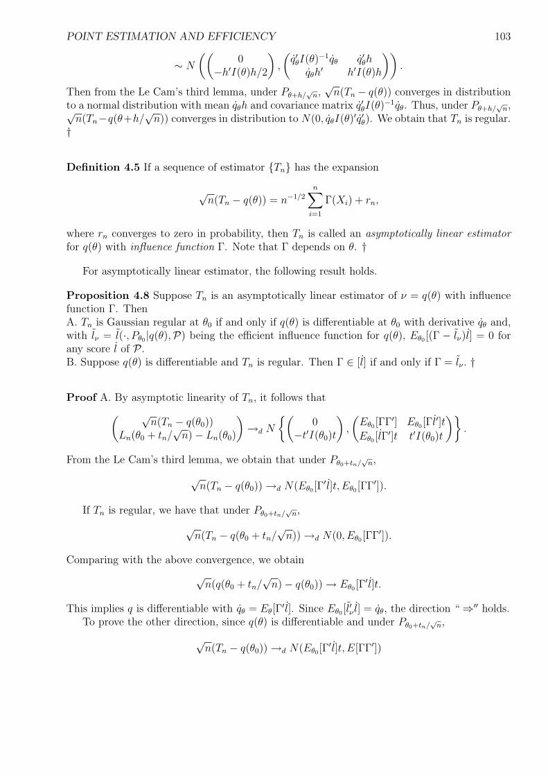
POINT ESTIMATION AND EFFICIENCY 103
∼ N
((0
−h′I(θ)h/2
),
(q′θI(θ)−1qθ q′θh
qθh′ h′I(θ)h
)).
Then from the Le Cam’s third lemma, under Pθ+h/√
n,√
n(Tn − q(θ)) converges in distributionto a normal distribution with mean qθh and covariance matrix q′θI(θ)−1qθ. Thus, under Pθ+h/
√n,√
n(Tn−q(θ+h/√
n)) converges in distribution to N(0, qθI(θ)′q′θ). We obtain that Tn is regular.†
Definition 4.5 If a sequence of estimator Tn has the expansion
√n(Tn − q(θ)) = n−1/2
n∑i=1
Γ(Xi) + rn,
where rn converges to zero in probability, then Tn is called an asymptotically linear estimatorfor q(θ) with influence function Γ. Note that Γ depends on θ. †
For asymptotically linear estimator, the following result holds.
Proposition 4.8 Suppose Tn is an asymptotically linear estimator of ν = q(θ) with influencefunction Γ. ThenA. Tn is Gaussian regular at θ0 if and only if q(θ) is differentiable at θ0 with derivative qθ and,with lν = l(·, Pθ0|q(θ),P) being the efficient influence function for q(θ), Eθ0 [(Γ − lν)l] = 0 forany score l of P .B. Suppose q(θ) is differentiable and Tn is regular. Then Γ ∈ [l] if and only if Γ = lν . †
Proof A. By asymptotic linearity of Tn, it follows that
( √n(Tn − q(θ0))
Ln(θ0 + tn/√
n)− Ln(θ0)
)→d N
(0
−t′I(θ0)t
),
(Eθ0 [ΓΓ′] Eθ0 [Γl′]tEθ0 [lΓ
′]t t′I(θ0)t
).
From the Le Cam’s third lemma, we obtain that under Pθ0+tn/√
n,
√n(Tn − q(θ0)) →d N(Eθ0 [Γ
′l]t, Eθ0 [ΓΓ′]).
If Tn is regular, we have that under Pθ0+tn/√
n,
√n(Tn − q(θ0 + tn/
√n)) →d N(0, Eθ0 [ΓΓ′]).
Comparing with the above convergence, we obtain
√n(q(θ0 + tn/
√n)− q(θ0)) → Eθ0 [Γ
′l]t.
This implies q is differentiable with qθ = Eθ[Γ′l]. Since Eθ0 [l
′ν l] = qθ, the direction “ ⇒′′ holds.
To prove the other direction, since q(θ) is differentiable and under Pθ0+tn/√
n,
√n(Tn − q(θ0)) →d N(Eθ0 [Γ
′l]t, E[ΓΓ′])
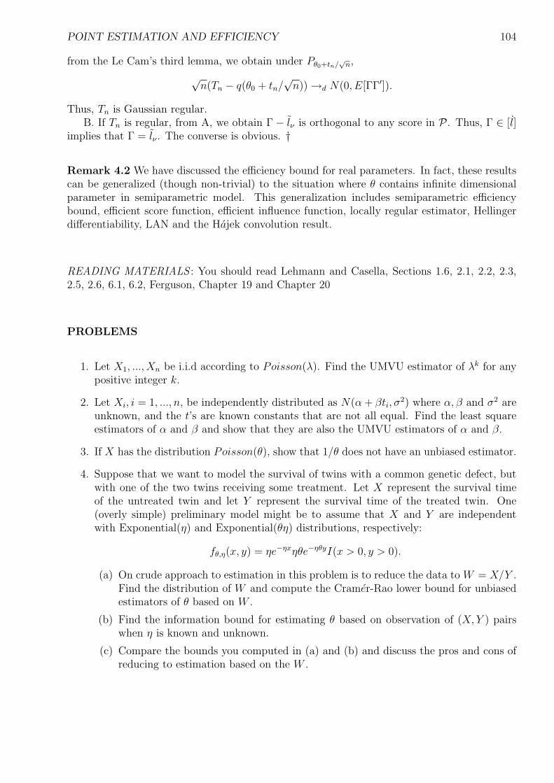
POINT ESTIMATION AND EFFICIENCY 104
from the Le Cam’s third lemma, we obtain under Pθ0+tn/√
n,
√n(Tn − q(θ0 + tn/
√n)) →d N(0, E[ΓΓ′]).
Thus, Tn is Gaussian regular.B. If Tn is regular, from A, we obtain Γ− lν is orthogonal to any score in P . Thus, Γ ∈ [l]
implies that Γ = lν . The converse is obvious. †
Remark 4.2 We have discussed the efficiency bound for real parameters. In fact, these resultscan be generalized (though non-trivial) to the situation where θ contains infinite dimensionalparameter in semiparametric model. This generalization includes semiparametric efficiencybound, efficient score function, efficient influence function, locally regular estimator, Hellingerdifferentiability, LAN and the Hajek convolution result.
READING MATERIALS : You should read Lehmann and Casella, Sections 1.6, 2.1, 2.2, 2.3,2.5, 2.6, 6.1, 6.2, Ferguson, Chapter 19 and Chapter 20
PROBLEMS
1. Let X1, ..., Xn be i.i.d according to Poisson(λ). Find the UMVU estimator of λk for anypositive integer k.
2. Let Xi, i = 1, ..., n, be independently distributed as N(α + βti, σ2) where α, β and σ2 are
unknown, and the t’s are known constants that are not all equal. Find the least squareestimators of α and β and show that they are also the UMVU estimators of α and β.
3. If X has the distribution Poisson(θ), show that 1/θ does not have an unbiased estimator.
4. Suppose that we want to model the survival of twins with a common genetic defect, butwith one of the two twins receiving some treatment. Let X represent the survival timeof the untreated twin and let Y represent the survival time of the treated twin. One(overly simple) preliminary model might be to assume that X and Y are independentwith Exponential(η) and Exponential(θη) distributions, respectively:
fθ,η(x, y) = ηe−ηxηθe−ηθyI(x > 0, y > 0).
(a) On crude approach to estimation in this problem is to reduce the data to W = X/Y .Find the distribution of W and compute the Cramer-Rao lower bound for unbiasedestimators of θ based on W .
(b) Find the information bound for estimating θ based on observation of (X,Y ) pairswhen η is known and unknown.
(c) Compare the bounds you computed in (a) and (b) and discuss the pros and cons ofreducing to estimation based on the W .
POINT ESTIMATION AND EFFICIENCY 105
5. This is a continuation of the preceding problem. A more realistic model involves assumingthat the common parameter η for the two wins varies across sets of twins. There are severaldifferent ways of modeling this: one approach involves supposing that each pair of twinsobserved (Xi, Yi) has its own fixed parameters ηi, i = 1, .., n. In this model we observe(Xi, Yi) with density fθ,ηi
for i = 1, ..., n; i.e.,
fθ,ηi(x, y) = ηie
−ηixiηiθe−ηiθyiI(xi > 0, yi > 0).
This is sometimes called a functional model (or model with incidental nuisance parame-ters).Another approach is to assume that η ≡ Z has a distribution, and that our obser-vations are from the mixture distribution. Assuming (for simplicity) that Z = η ∼Gamma(a, 1/b) (a and b are known) with density
ga,b(η) =baηa−1
Γ(a)exp−bηI(η > 0),
it follows that the (marginal) distribution of (X, Y ) is
pθ,a,b(x, y) =
∫ ∞
0
fθ,z(x, y)ga,b(z)dz.
This is sometimes called a “structural model” (or mixture model).
(a) Find the information bound for θ in the functional model based on (Xi, Yi), i =1, ..., n.
(b) Find the information bound for θ in the structural model based on (Xi, Yi), i =1, ..., n.
(c) Compare the information bounds you computed in (a) and (b). When is the informa-tion for θ in the functional model larger than the information for θ in the structuralmodel?
6. Suppose that X ∼ Gamma(α, 1/β); i.e., X has density pθ given by
pθ(x) =βα
Γ(α)xα−1 exp−βxI(x > 0), θ = (α, β) ∈ (0,∞)× (0,∞).
Consider estimation of q(θ) = Eθ[X].
(a) Compute the Fisher information matrix I(θ).
(b) Derive the efficient score function, the efficient influence function and the efficientinformation bound for α.
(c) Compute q(θ) and find the efficient influence functions for estimation of q(θ). Com-pare the efficient influence functions you find in (c) with the influence function ofthe natural estimator Xn.
7. Compute the score for location, −(f ′/f)(x), and the Fisher information when:
POINT ESTIMATION AND EFFICIENCY 106
(a) f(x) = φ(x) = (2π)−1/2 exp−x2/2, (normal or Gaussian);
(b) f(x) = exp−x/(1 + exp−x)2, (logistic);
(c) f(x) = exp−|x|/2, (double exponential);
(d) f(x) = tk, the t-distribution with k degrees of freedom;
(e) f(x) = exp−x exp− exp(−x), (Gumbel or extreme value).
8. Suppose that P = Pθ : θ ∈ Θ , Θ ⊂ Rk is a parametric model satisfying the hypothesesof the multiparameter Crameer-Rao inequality. Partition θ as θ = (ν, η), where ν ∈ Rm
and η ∈ Rk−m and 1 ≤ m < k. Let l = lθ = (l1, l2) be the corresponding partition of thescores and with l = I−1(θ)l, the efficient influence function for θ, let l = (l1, l2) be thecorresponding partition of l. In both cases, l1, l1 are m-vectors of functions and l2, l2 arek −m vectors. Partition I(θ) and I−1(θ) correspondingly as
I(θ) =
(I11 I12
I21 I22
),
where I11 is m×m, I12 is m× (k−m), I21 is (k−m)×m, I22 is (k−m)× (k−m). alsowrite
I−1(θ) = [I ij]i,j=1,2.
Verify that
(a) I11 = I−111·2 where I11·2 = I11 − I12I
−122 I21, I22 = I−1
22·1 where I22·1 = I22 − I21I−111 I12,
I12 = −I−111·2I12I
−122 , I21 = −I22 · 1−1I21I
−111 ..
(b) Verify that l1 = I11l1 + I12l2 = I−111·2(l1 − I12I
−122 l2), and l2 = I21l1 + I22l2 = I−1
22·1(l2 −I21I
−111 l1).
9. Let Tn be the Hodges superefficient estimator of θ.
(a) Show that Tn is not a regular estimator of θ at θ = 0, but that it is regular at everyθ 6= 0. If θn = t/
√n, find the limiting distribution of
√n(Tn − θn) under Pθn .
(b) For θn = t/√
n show that
Rn(θn) = nEθn [(Tn − θn)2] → a2 + t2(1− a)2.
This is larger than 1 if t2 > (1 + a)/(1− a), and hence supper efficiency also entailsworse risks in a local neighborhood of the points where the asymptotic variance issmaller.
10. Suppose that (Y |Z) ∼ Weibull(λ−1 exp−γZ, β) and Z ∼ Gη on R with density gη withrespect to some dominating measure µ. Thus the conditional cumulative hazards functionΛ(t|z) is given by
Λγ,λ,β(t|z) = (λeγzt)β = λβeβγztβ
and henceλγ,λ,β(t|z) = λβeβγzβtβ−1.
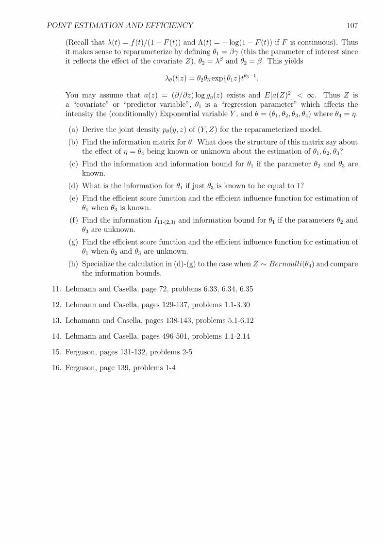
POINT ESTIMATION AND EFFICIENCY 107
(Recall that λ(t) = f(t)/(1− F (t)) and Λ(t) = − log(1− F (t)) if F is continuous). Thusit makes sense to reparameterize by defining θ1 = βγ (this the parameter of interest sinceit reflects the effect of the covariate Z), θ2 = λβ and θ2 = β. This yields
λθ(t|z) = θ2θ3 expθ1ztθ3−1.
You may assume that a(z) = (∂/∂z) log gη(z) exists and E[a(Z)2] < ∞. Thus Z isa “covariate” or “predictor variable”, θ1 is a “regression parameter” which affects theintensity the (conditionally) Exponential variable Y , and θ = (θ1, θ2, θ3, θ4) where θ4 = η.
(a) Derive the joint density pθ(y, z) of (Y, Z) for the reparameterized model.
(b) Find the information matrix for θ. What does the structure of this matrix say aboutthe effect of η = θ4 being known or unknown about the estimation of θ1, θ2, θ3?
(c) Find the information and information bound for θ1 if the parameter θ2 and θ3 areknown.
(d) What is the information for θ1 if just θ3 is known to be equal to 1?
(e) Find the efficient score function and the efficient influence function for estimation ofθ1 when θ3 is known.
(f) Find the information I11·(2,3) and information bound for θ1 if the parameters θ2 andθ3 are unknown.
(g) Find the efficient score function and the efficient influence function for estimation ofθ1 when θ2 and θ3 are unknown.
(h) Specialize the calculation in (d)-(g) to the case when Z ∼ Bernoulli(θ4) and comparethe information bounds.
11. Lehmann and Casella, page 72, problems 6.33, 6.34, 6.35
12. Lehmann and Casella, pages 129-137, problems 1.1-3.30
13. Lehamann and Casella, pages 138-143, problems 5.1-6.12
14. Lehmann and Casella, pages 496-501, problems 1.1-2.14
15. Ferguson, pages 131-132, problems 2-5
16. Ferguson, page 139, problems 1-4
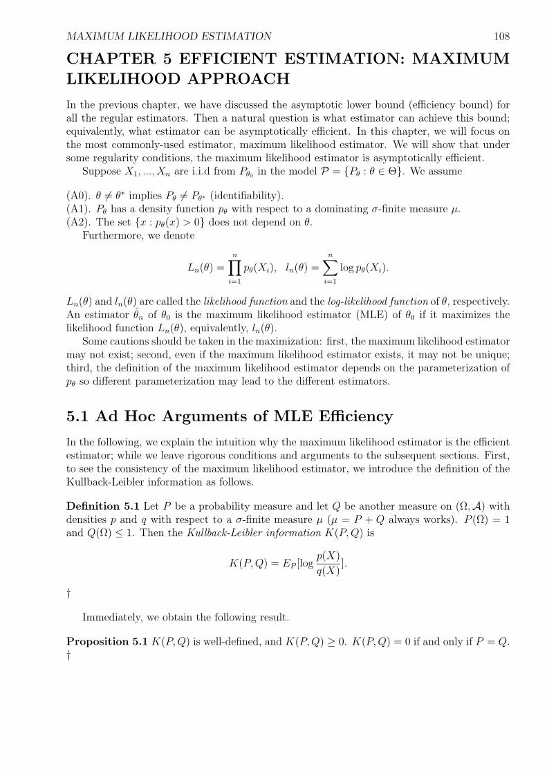
MAXIMUM LIKELIHOOD ESTIMATION 108
CHAPTER 5 EFFICIENT ESTIMATION: MAXIMUM
LIKELIHOOD APPROACH
In the previous chapter, we have discussed the asymptotic lower bound (efficiency bound) forall the regular estimators. Then a natural question is what estimator can achieve this bound;equivalently, what estimator can be asymptotically efficient. In this chapter, we will focus onthe most commonly-used estimator, maximum likelihood estimator. We will show that undersome regularity conditions, the maximum likelihood estimator is asymptotically efficient.
Suppose X1, ..., Xn are i.i.d from Pθ0 in the model P = Pθ : θ ∈ Θ. We assume
(A0). θ 6= θ∗ implies Pθ 6= Pθ∗ (identifiability).(A1). Pθ has a density function pθ with respect to a dominating σ-finite measure µ.(A2). The set x : pθ(x) > 0 does not depend on θ.
Furthermore, we denote
Ln(θ) =n∏
i=1
pθ(Xi), ln(θ) =n∑
i=1
log pθ(Xi).
Ln(θ) and ln(θ) are called the likelihood function and the log-likelihood function of θ, respectively.An estimator θn of θ0 is the maximum likelihood estimator (MLE) of θ0 if it maximizes thelikelihood function Ln(θ), equivalently, ln(θ).
Some cautions should be taken in the maximization: first, the maximum likelihood estimatormay not exist; second, even if the maximum likelihood estimator exists, it may not be unique;third, the definition of the maximum likelihood estimator depends on the parameterization ofpθ so different parameterization may lead to the different estimators.
5.1 Ad Hoc Arguments of MLE Efficiency
In the following, we explain the intuition why the maximum likelihood estimator is the efficientestimator; while we leave rigorous conditions and arguments to the subsequent sections. First,to see the consistency of the maximum likelihood estimator, we introduce the definition of theKullback-Leibler information as follows.
Definition 5.1 Let P be a probability measure and let Q be another measure on (Ω,A) withdensities p and q with respect to a σ-finite measure µ (µ = P + Q always works). P (Ω) = 1and Q(Ω) ≤ 1. Then the Kullback-Leibler information K(P,Q) is
K(P,Q) = EP [logp(X)
q(X)].
†
Immediately, we obtain the following result.
Proposition 5.1 K(P, Q) is well-defined, and K(P,Q) ≥ 0. K(P, Q) = 0 if and only if P = Q.†
MAXIMUM LIKELIHOOD ESTIMATION 109
Proof By the Jensen’s inequality,
K(P, Q) = EP [− logq(X)
p(X)] ≥ − log EP [
q(X)
p(X)] = − log Q(Ω) ≥ 0.
The equality holds if and only if p(x) = Mq(x) almost surely with respect P and Q(Ω) = 1.Thus, M = 1 and P = Q. †
Now that θn maximizes ln(θ),
1
n
n∑i=1
pθn(Xi) ≥ 1
n
n∑i=1
pθ0(Xi).
Suppose θn → θ∗. Then we would expect to the both sides converge to
Eθ0 [pθ∗(X)] ≥ Eθ0 [pθ0(X)],
which implies K(Pθ0 , Pθ∗) ≤ 0. From Proposition 5.1, Pθ0 = Pθ∗ . From (A0), θ∗ = θ0 (the modelidentifiability condition is used here). That is, θn converges to θ0. Note in this argument, threeconditions are essential: (i) θn → θ∗ (compactness of θn); (ii) the convergence of n−1ln(θn)(locally uniform convergence); (iii) Pθ0 = Pθ∗ implies θ0 = θ∗ (identifiability).
Next, we give an ad hoc discussion on the efficiency of the maximum likelihood estimator.Suppose θn → θ0. If θn is in the interior of Θ, θn solves the following likelihood (or score)equations
ln(θn) =n∑
i=1
lθn(Xi) = 0.
Suppose lθ(X) is twice-differentiable with respect to θ. We apply the Taylor expansion tolθn
(Xi) at θ0 and obtain
−n∑
i=1
lθ0(Xi) =n∑
i=1
lθ∗(Xi)(θ − θ0),
where θ∗ is between θ0 and θ. This gives that
√n(θ − θ0) = − 1√
n
n−1
n∑i=1
lθ∗(Xi)
−1 n∑
i=1
lθ0(Xi)
.
By the law of large number, we can see√
n(θn − θ0) is asymptotically equivalent to
1√n
n∑i=1
I(θ0)−1lθ0(Xi).
Then θn is an asymptotically linear estimator of θ0 with the influence function I(θ0)−1lθ0 =
l(·, Pθ0|θ,P). This shows that θn is the efficient estimator of θ0 and the asymptotic variance of√n(θn − θ0) attains the efficiency bound, which was defined in the previous chapter. Again,
the above arguments require a few conditions to go through.As mentioned before, in the following sections we will rigorously prove the consistency and
the asymptotic efficiency of the maximum likelihood estimator. Moreover, we will discuss thecomputation of the maximum likelihood estimators and some alternative efficient estimationapproaches.
MAXIMUM LIKELIHOOD ESTIMATION 110
5.2 Consistency of Maximum Likelihood Estimator
We provide some sufficient conditions for obtaining the consistency of maximum likelihoodestimator.
Theorem 5.1 Suppose that(a) Θ is compact.(b) log pθ(x) is continuous in θ for all x.(c) There exists a function F (x) such that Eθ0 [F (X)] < ∞ and | log pθ(x)| ≤ F (x) for all x andθ.Then θn →a.s. θ0. †
Proof For any sample ω ∈ Ω, θn is compact. Thus, be choosing a subsequence, we assumeθn → θ∗. Suppose we can show that
1
n
n∑i=1
lθn(Xi) → Eθ0 [lθ∗(X)].
Then since1
n
n∑i=1
lθn(Xi) ≥ 1
n
n∑i=1
lθ0(Xi),
we haveEθ0 [lθ∗(X)] ≥ Eθ0 [lθ0(X)].
Thus Proposition 5.1 plus the identifiability gives θ∗ = θ0. That is, any subsequence of θn
converges to θ0. We conclude that θn →a.s. θ0.It remains to show
Pn[lθn(X)] ≡ 1
n
n∑i=1
lθn(Xi) → Eθ0 [lθ∗(X)].
SinceEθ0 [lθn
(X)] → Eθ0 [lθ∗(X)]
by the dominated convergence theorem, it suffices to show
|Pn[lθn(X)]− Eθ0 [lθn
(X)]| → 0.
We can even prove the following uniform convergence result
supθ∈Θ
|Pn[lθ(X)]− Eθ0 [lθ(X)]| → 0.
To see this, we defineψ(x, θ, ρ) = sup
|θ′−θ|<ρ
(lθ′(x)− Eθ0 [lθ′(X)]).
Since lθ is continuous, ψ(x, θ, ρ) is measurable and by the dominance convergence theorem,Eθ0 [ψ(X, θ, ρ)] decreases to Eθ0 [lθ(x) − Eθ0 [lθ(X)]] = 0. Thus, for ε > 0, for any θ ∈ Θ, thereexists a ρθ such that
Eθ0 [ψ(X, θ, ρθ)] < ε.
MAXIMUM LIKELIHOOD ESTIMATION 111
The union of θ′ : |θ′−θ| < ρθ covers Θ. By the compactness of Θ, there exists a finite numberof θ1, ..., θm such that
Θ ⊂ ∪mi=1θ′ : |θ′ − θi| < ρθi
.Therefore,
supθ∈Θ
Pn[lθ(X)]− Eθ0 [lθ(X)] ≤ sup1≤i≤m
Pn[ψ(X, θi, ρθi)].
We obtain
lim supn
supθ∈Θ
Pn[lθ(X)]− Eθ0 [lθ(X)] ≤ sup1≤i≤m
Pθ[ψ(X, θi, ρθi)] ≤ ε.
Thus, lim supn supθ∈Θ Pn[lθ(X)]− Eθ0 [lθ(X)] ≤ 0. We apply the similar arguments to −l(X, θ)and obtain lim supn supθ∈Θ −Pn[lθ(X)] + Eθ0 [lθ(X)] ≤ 0. Thus,
limn
supθ∈Θ
|Pn[lθ(X)]− Eθ0 [lθ(X)]| → 0.
†
As a note, condition (c) in Theorem 5.1 is necessary. Ferguson (2002) page 116 gives aninteresting counterexample showing that if (c) is invalid, the maximum likelihood estimatorconverges to a fixed constant whatever true parameter is.
Another type of consistency result is the classical Wald’s consistency result.
Theorem 5.2 (Wald’s Consistency) Θ is compact. Suppose θ 7→ lθ(x) = log pθ(x) is upper-semicontinuous for all x, in the sense
lim supθ′→θ
lθ′(x) ≤ lθ(x).
Suppose for every sufficient small ball U ⊂ Θ,
Eθ0 [supθ′∈U
lθ′(X)] < ∞.
Then θn →p θ0. †
Proof Since Eθ0 [lθ0(X)] > Eθ0 [lθ′(X)] for any θ′ 6= θ0, there exists a ball Uθ′ containing θ′ suchthat
Eθ0 [lθ0(X)] > Eθ0 [ supθ∗∈Uθ′
lθ∗(X)].
Otherwise, there exists a sequence θ∗m → θ′ but Eθ0 [lθ0(X)] ≤ Eθ0 [lθ∗m(X)]. Since lθ∗m(x) ≤supU ′ lθ′(X) where U ′ is the ball satisfying the condition, we obtain
lim supm
Eθ0 [lθ∗m(X)] ≤ Eθ0 [lim supm
lθ∗m(X)] ≤ Eθ0 [lθ′(X)].
We then obtain Eθ0 [lθ0(X)] ≤ Eθ0 [lθ′(X)] and this is a contradiction.
MAXIMUM LIKELIHOOD ESTIMATION 112
For any ε, the balls ∪θ′Uθ′ covers the compact set Θ∩ |θ′ − θ0| > ε so there exists a finitecovering balls, U1, ..., Um. Then
P (|θn− θ0| > ε) ≤ P ( sup|θ′−θ0|>ε
Pn[lθ′(X)] ≥ Pn[lθ0(X)]) ≤ P ( max1≤i≤m
Pn[ supθ′∈Ui
lθ′(X)] ≥ Pn[lθ0(X)])
≤m∑
i=1
P (Pn[ supθ′∈Ui
lθ′(X)] ≥ Pn[lθ0(X)]).
SincePn[ sup
θ′∈Ui
lθ′(X)] →a.s. Eθ0 [ supθ′∈Ui
lθ′(X)] < Eθ0 [lθ0(X)],
the right-hand side converges to zero. Thus, θn →p θ0. †
5.3. Asymptotic Efficiency of Maximum Likelihood Esti-
mator
The following theorem gives some regular conditions so that the maximum likelihood estimatorattains asymptotic efficiency bound.
Theorem 5.3 Suppose that the model P = Pθ : θ ∈ Θ is Hellinger differentiable at an innerpoint θ0 of Θ ⊂ Rk. Furthermore, suppose that there exists a measurable function F (X) withEθ0 [F (X)2] < ∞ such that for every θ1 and θ2 in a neighborhood of θ0,
| log pθ1(x)− log pθ2(x)| ≤ F (x)|θ1 − θ2|.
If the Fisher information matrix I(θ0) is nonsingular and θn is consistent, then
√n(θn − θ0) =
1√n
n∑i=1
I(θ0)−1lθ0(Xi) + op(1).
In particular,√
n(θn − θ0) is asymptotically normal with mean zero and covariance matrixI(θ0)
−1.†
Proof For any hn → h, by the Hellinger differentiability,
Wn = 2
(√pθ0+hn/
√n
pθ0
− 1
)→ h′lθ0 , in L2(Pθ0).
We obtain √n(log pθ0+hn/
√n − log pθ0) = 2
√n log(1 + Wn/2) →p h′lθ0 .
Using the Lipschitz continuity of log pθ and the dominate convergence theorem, we can show
Eθ0
[√n(Pn − P )[
√n(log pθ0+hn/
√n − log pθ0)− h′lθ0 ]
]→ 0
MAXIMUM LIKELIHOOD ESTIMATION 113
andV arθ0
[√n(Pn − P )[
√n(log pθ0+hn/
√n − log pθ0)− h′lθ0 ]
]→ 0.
Thus, √n(Pn − P )[
√n(log pθ0+hn/
√n − log pθ0)− h′lθ0 ] →p 0,
where√
n(Pn − P )[g(X)] is defined as
n−1/2
[n∑
i=1
g(Xi)− Eθ0 [g(X)]]
.
From Step I in proving Theorem 4.4, we know
logn∏
i=1
log pθ0+hn/√
n
log pθ0
=1√n
n∑i=1
h′lθ0(Xi)− 1
2h′I(θ0)h + op(1).
We obtainnEθ0 [log pθ0+hn/
√n − log pθ0 ] → −h′I(θ0)h/2.
Hence the map θ 7→ Eθ0 [log pθ] is twice-differentiable with second derivative matrix −I(θ0).Furthermore, we obtain
nPn[log pθ0+hn/√
n − log pθ0 ] = −1
2h′nI(θ0)hn + h′n
√n(Pn − P )[lθ0 ] + op(1).
We choose hn =√
n(θn − θ0) and hn = I(θ0)−1√
n(Pn − P )[lθ0 ]. It gives that
nPn[log pθn− log pθ0 ] = −n
2(θn − θ0)
′I(θ0)(θ − θ0) +√
n(θn − θ0)√
n(Pn − P )[lθ0 ] + op(1),
nPn[log pθ0+I(θ0)−1√
n(Pn−P )[lθ0 ]/√
n − log pθ0 ]
=1
2√n(Pn − P )[lθ0 ]′I(θ0)
−1√n(Pn − P )[lθ0 ]+ op(1).
Since the left-hand side of the fist equation is larger than the left-hand side of the secondequation, after simple algebra, we obtain
−1
2
√n(θn − θ0)− I(θ0)
−1√
n(Pn − P )[lθ0 ]′
I(θ0)√
n(θn − θ0)− I(θ0)−1√
n(Pn − P )[lθ0 ]
+op(1) ≥ 0.
Thus, √n(θn − θ0) = I(θ0)
−1√
n(Pn − P )[lθ0 ] + op(1).
†
A classical condition for the asymptotic normality for√
n(θn− θ0) is the following theorem.
Theorem 5.4 For each θ in an open subset of Euclidean space. Let θ 7→ lθ(x) = log pθ(x)be twice continuously differentiable for every x. Suppose Eθ0 [lθ0 l
′θ0
] < ∞ and E[lθ0 ] exists and
MAXIMUM LIKELIHOOD ESTIMATION 114
is nonsingular. Assume that the second partial derivative of lθ(x) is dominated by a fixedintegrable function F (x) for every θ in a neighborhood of θ0. Suppose θn →p θ0. Then
√n(θn − θ0) = −(Eθ0 [lθ0 ])
−1 1√n
n∑i=1
lθ0(Xi) + op(1).
†
Proof θn solves the equation
0 =n∑
i=1
lθ(Xi).
After the Taylor expansion, we obtain
0 =n∑
i=1
lθ0(Xi) +n∑
i=1
lθ0(Xi)(θn − θ0) +1
2(θn − θ0)
′
n∑i=1
l(3)
θn(Xi)
(θn − θ0),
where θn is between θn and θ0. Thus,
|
1
n
n∑i=1
lθ0(Xi)
(θn − θ0) +
1
n
n∑i=1
lθ0(Xi)| ≤ 1
n
n∑i=1
|F (Xi)||θn − θ0|2.
We obtain (θn − θ0) = op(1/√
n). Then it holds
√n(θn − θ0)
1
n
n∑i=1
lθ0(Xi) + op(1)
= − 1√
n
n∑i=1
lθ0(Xi).
The result holds. † .
5.4 Computation of Maximum Likelihood Estimate
A variety of methods can be used to compute the maximum likelihood estimate. Since themaximum likelihood estimate, θn, solves the likelihood equation
n∑i=1
lθ(Xi) = 0,
one numerical method for the calculation is via the Newton-Raphson iteration: at kth iteration,
θ(k+1) = θ(k) −
1
n
n∑i=1
lθ(k)(Xi)
−1 1
n
n∑i=1
lθ(k)(Xi)
.
Sometimes, calculating lθ may be complicated. Note the
− 1
n
n∑i=1
lθ(k)(Xi) ≈ I(θ(k)).
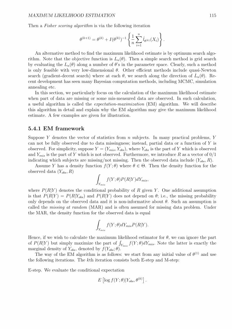
MAXIMUM LIKELIHOOD ESTIMATION 115
Then a Fisher scoring algorithm is via the following iteration
θ(k+1) = θ(k) + I(θ(k))−1
1
n
n∑i=1
lθ(k)(Xi)
.
An alternative method to find the maximum likelihood estimate is by optimum search algo-rithm. Note that the objective function is Ln(θ). Then a simple search method is grid searchby evaluating the Ln(θ) along a number of θ’s in the parameter space. Clearly, such a methodis only feasible with very low-dimensional θ. Other efficient methods include quasi-Newtonsearch (gradient-decent search) where at each θ, we search along the direction of Ln(θ). Re-cent development has seen many Bayesian computation methods, including MCMC, simulationannealing etc.
In this section, we particularly focus on the calculation of the maximum likelihood estimatewhen part of data are missing or some mis-measured data are observed. In such calculation,a useful algorithm is called the expectation-maximization (EM) algorithm. We will describethis algorithm in detail and explain why the EM algorithm may give the maximum likelihoodestimate. A few examples are given for illustration.
5.4.1 EM framework
Suppose Y denotes the vector of statistics from n subjects. In many practical problems, Ycan not be fully observed due to data missingness; instead, partial data or a function of Y isobserved. For simplicity, suppose Y = (Ymis, Yobs), where Yobs is the part of Y which is observedand Ymis is the part of Y which is not observed. Furthermore, we introduce R as a vector of 0/1indicating which subjects are missing/not missing. Then the observed data include (Yobs, R).
Assume Y has a density function f(Y ; θ) where θ ∈ Θ. Then the density function for theobserved data (Yobs, R) ∫
Ymis
f(Y ; θ)P (R|Y )dYmis,
where P (R|Y ) denotes the conditional probability of R given Y . One additional assumptionis that P (R|Y ) = P (R|Yobs) and P (R|Y ) does not depend on θ; i.e., the missing probabilityonly depends on the observed data and it is non-informative about θ. Such an assumption iscalled the missing at random (MAR) and is often assumed for missing data problem. Underthe MAR, the density function for the observed data is equal
∫
Ymis
f(Y ; θ)dYmisP (R|Y ).
Hence, if we wish to calculate the maximum likelihood estimator for θ, we can ignore the partof P (R|Y ) but simply maximize the part of
∫Ymis
f(Y ; θ)dYmis. Note the latter is exactly themarginal density of Yobs, denoted by f(Yobs; θ).
The way of the EM algorithm is as follows: we start from any initial value of θ(1) and usethe following iterations. The kth iteration consists both E-step and M-step:
E-step. We evaluate the conditional expectation
E[log f(Y ; θ)|Yobs, θ
(k)].
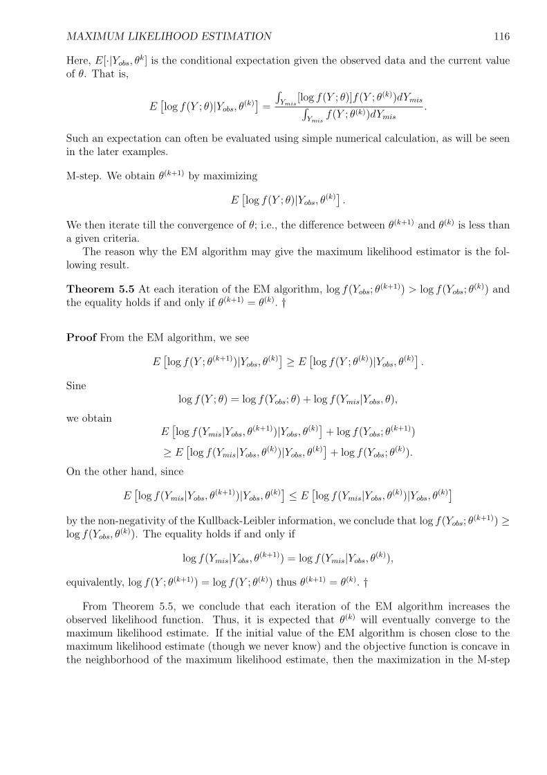
MAXIMUM LIKELIHOOD ESTIMATION 116
Here, E[·|Yobs, θk] is the conditional expectation given the observed data and the current value
of θ. That is,
E[log f(Y ; θ)|Yobs, θ
(k)]
=
∫Ymis
[log f(Y ; θ)]f(Y ; θ(k))dYmis∫Ymis
f(Y ; θ(k))dYmis
.
Such an expectation can often be evaluated using simple numerical calculation, as will be seenin the later examples.
M-step. We obtain θ(k+1) by maximizing
E[log f(Y ; θ)|Yobs, θ
(k)].
We then iterate till the convergence of θ; i.e., the difference between θ(k+1) and θ(k) is less thana given criteria.
The reason why the EM algorithm may give the maximum likelihood estimator is the fol-lowing result.
Theorem 5.5 At each iteration of the EM algorithm, log f(Yobs; θ(k+1)) > log f(Yobs; θ
(k)) andthe equality holds if and only if θ(k+1) = θ(k). †
Proof From the EM algorithm, we see
E[log f(Y ; θ(k+1))|Yobs, θ
(k)] ≥ E
[log f(Y ; θ(k))|Yobs, θ
(k)].
Sinelog f(Y ; θ) = log f(Yobs; θ) + log f(Ymis|Yobs, θ),
we obtainE
[log f(Ymis|Yobs, θ
(k+1))|Yobs, θ(k)
]+ log f(Yobs; θ
(k+1))
≥ E[log f(Ymis|Yobs, θ
(k))|Yobs, θ(k)
]+ log f(Yobs; θ
(k)).
On the other hand, since
E[log f(Ymis|Yobs, θ
(k+1))|Yobs, θ(k)
] ≤ E[log f(Ymis|Yobs, θ
(k))|Yobs, θ(k)
]
by the non-negativity of the Kullback-Leibler information, we conclude that log f(Yobs; θ(k+1)) ≥
log f(Yobs, θ(k)). The equality holds if and only if
log f(Ymis|Yobs, θ(k+1)) = log f(Ymis|Yobs, θ
(k)),
equivalently, log f(Y ; θ(k+1)) = log f(Y ; θ(k)) thus θ(k+1) = θ(k). †
From Theorem 5.5, we conclude that each iteration of the EM algorithm increases theobserved likelihood function. Thus, it is expected that θ(k) will eventually converge to themaximum likelihood estimate. If the initial value of the EM algorithm is chosen close to themaximum likelihood estimate (though we never know) and the objective function is concave inthe neighborhood of the maximum likelihood estimate, then the maximization in the M-step
MAXIMUM LIKELIHOOD ESTIMATION 117
can be replaced by the Newton-Raphson iteration. Correspondingly, an alternative way to theEM algorithm is given by:
E-step. We evaluate the conditional expectation
E
[∂
∂θlog f(Y ; θ)|Yobs, θ
(k)
]
and
E
[∂2
∂θ2log f(Y ; θ)|Yobs, θ
(k)
]
M-step. We obtain θ(k+1) by solving
0 = E
[∂
∂θlog f(Y ; θ)|Yobs, θ
(k)
]
using one-step Newton-Raphson iteration:
θ(k+1) = θ(k) −
E
[∂2
∂θ2log f(Y ; θ)|Yobs, θ
(k)
]−1
E
[∂
∂θlog f(Y ; θ)|Yobs, θ
(k)
]∣∣∣∣∣θ=θ(k)
.
We note that in the second form of the EM algorithm, only one-step Newton-Raphson iterationis used in the M-step since it still ensures that the iteration will increase the likelihood function.
5.4.2 Examples of using EM algorithm
Example 5.1 Suppose a random vector Y has a multinomial distribution with n = 197 and
p = (1
2+
θ
4,1− θ
4,1− θ
4,θ
4).
Then the probability for Y = (y1, y2, y3, y4) is given by
n!
y1!y2!y3!y4!(1
2+
θ
4)y1(
1− θ
4)y2(
1− θ
4)y3(
θ
4)y4 .
If we use the Newton-Raphson iteration to calculate the maximum likelihood estimator forθ, then after calculating the first and the second derivative of the log-likelihood function, weiterate using
θ(k+1) = θ(k) +
Y1
1/16
(1/2 + θ(k)/4)2+ (Y2 + Y3)
1
(1− θ(k))2+ Y4
1
θ(k)2
−1
×
Y11/4
1/2 + θ(k)/4− (Y2 + Y3)
1
1− θ(k)+ Y4
1
θ(k)
.
Suppose we observe Y = (125, 18, 20, 34). If we start with θ(1) = 0.5, after the convergence, weobtain θ(k) = 0.6268215. We can use the EM algorithm to calculate the maximum likelihood
MAXIMUM LIKELIHOOD ESTIMATION 118
estimator. Suppose the full data is X which has a multivariate normal distribution with n andthe p = (1/2, θ/4, (1 − θ)/4, (1 − θ)/4, θ/4). Then Y can be treated as an incomplete data ofX by Y = (X1 + X2, X3, X4, X5). The score equation for the complete data X is simple
0 =X2 + X5
θ− X3 + X4
1− θ.
Thus we note the M-step of the EM algorithm needs to solve the equation
0 = E
[X2 + X5
θ− X3 + X4
1− θ|Y, θ(k)
];
while the E-step evaluates the above expectation. By simple calculation,
E[X|Y, θ(k)] = (Y11/2
1/2 + θ(k)/4, Y1
θ(k)/4
1/2 + θ(k)/4, Y2, Y3, Y4).
Then we obtain
θ(k+1) =E[X2 + X5|Y, θ(k)]
E[X2 + X5 + X3 + X4|Y, θ(k)]=
Y1θ(k)/4
1/2+θ(k)/4+ Y4
Y1θ(k)/4
1/2+θ(k)/4+ Y2 + Y3 + Y4
.
We start form θ(1) = 0.5. The following table gives the results from iterations:
k θ(k+1) θ(k+1) − θ(k) θ(k+1)−θn
θ(k)−θn
0 .500000000 .126821498 .14651 .608247423 .018574075 .13462 .624321051 .002500447 .13303 .626488879 .000332619 .13284 .626777323 .000044176 .13285 .626815632 .000005866 .13286 .626820719 .0000007797 .626821395 .0000001048 .626821484 .000000014
From the table, we find the EM converges and the result agrees with what is obtained form theNewton-Raphson iteration. We also note the the convergence is linear as (θ(k+1) − θn)/(θ(k) − θn)becomes a constant when convergence; comparatively, the convergence in the Newton-Raphsoniteration is quadratic in the sense (θ(k+1) − θn)/(θ(k) − θn)2 becomes a constant when conver-gence. Thus, the Newton-Raphon iteration converges much faster than the EM algorithm;however, we have already seen the calculation of the EM is much less complex than the Newton-Raphson iteration and this is the advantage of using the EM algorithm.
Example 5.2 We consider the example of exponential mixture model. Suppose Y ∼ Pθ wherePθ has density
pθ(y) =pλe−λy + (1− p)µe−µy
I(y > 0)
and θ = (p, λ, µ) ∈ (0, 1) × (0,∞) × (0,∞). Consider estimation of θ based on Y1, ..., Yn
i.i.d pθ(y). Solving the likelihood equation using the Newton-Raphson is much computation
MAXIMUM LIKELIHOOD ESTIMATION 119
involved. We take an approach based on the EM algorithm. We introduce the complete dataX = (Y, ∆) ∼ pθ(x) where
pθ(x) = pθ(y, δ) = (pye−λy)δ((1− p)µe−µy)1−δ.
This is natural from the following mechanism: ∆ is a bernoulli variable with P (∆ = 1) = pand we generate Y from Exp(λ) if ∆ = 1 and from Exp(µ) if ∆ = 0. Thus, ∆ is missing. Thescore equation for θ based on X is equal to
0 = lp(X1, ..., Xn) =n∑
i=1
∆i
p− 1−∆i
1− p
,
0 = lλ(X1, ..., Xn) =n∑
i=1
∆i(1
λ− Yi),
0 = lµ(X1, ..., Xn) =n∑
i=1
(1−∆i)(1
µ− Yi).
Thus, the M-step of the EM algorithm is to solve the following equations
0 =n∑
i=1
E
[∆i
p− 1−∆i
1− p
|Y1, ..., Yn, p(k), λ(k), µ(k)
]=
n∑i=1
E
[∆i
p− 1−∆i
1− p
|Yi, p
(k), λ(k), µ(k)
],
0 =n∑
i=1
E
[∆i(
1
λ− Yi)|Y1, ..., Yn, p(k), λ(k), µ(k)
]=
n∑i=1
E
[∆i(
1
λ− Yi)|Yi, p
(k), λ(k), µ(k)
],
0 =n∑
i=1
E
[1−∆i)(
1
µ− Yi)|Y1, ..., Yn, p
(k), λ(k), µ(k)
]=
n∑i=1
E
[1−∆i)(
1
µ− Yi)|Yi, p
(k), λ(k), µ(k)
].
This immediately gives
p(k+1) =1
n
n∑i=1
E[∆i|Yi, p(k), λ(k), µ(k)],
λ(k+1) =
∑ni=1 E[∆i|Yi, p
(k), λ(k), µ(k)]∑ni=1 YiE[∆i|Yi, p(k), λ(k), µ(k)]
,
µ(k+1) =
∑ni=1 E[(1−∆i)|Yi, p
(k), λ(k), µ(k)]∑ni=1 YiE[(1−∆i)|Yi, p(k), λ(k), µ(k)]
.
The conditional expectation
E[∆|Y, θ] =pλe−λY
pλe−λY + (1− p)µe−µY.
As seen above, the EM algorithm facilitates the computation.
MAXIMUM LIKELIHOOD ESTIMATION 120
5.4.3 Information calculation in EM algorithm
We now consider the information of θ in the missing data. Denote lc as the score functionfor θ in the full data and denote lmis|obs as the score for θ in the conditional distribution of
Ymis given Yobs and lobs as the the score for θ in the distribution of Yobs. Then it is clear thatlc = lmis|obs + lobs. Using the formula
V ar(U) = V ar(E[U |V ]) + E[V ar(U |V )],
we obtainV ar(lc) = V ar(E[lc|Yobs]) + E[V ar(lc|Yobs)].
SinceE[lc|Yobs] = lobs + E[lmis|obs|Yobs] = lobs
andV ar(lc|Yobs) = V ar(lmis|obs|Yobs),
we obtainV ar(lc) = V ar(lobs) + E[V ar(lmis|obs|Yobs)].
Note that V ar(lc) is the information for θ based the complete data Y , denote by Ic(θ),V ar(lobs) is the information for θ based on the observed data Yobs, denote by Iobs(θ), andthe V ar(lmis|obs|Yobs) is the conditional information for θ based on Ymis given Yobs, denoted byImis|obs(θ; Yobs). We obtain the following Louis formula
Ic(θ) = Iobs(θ) + E[Imis|obs(θ, Yobs)].
Thus, the complete information is the summation of the observed information and the missinginformation. One can even show when the EM converges, the convergence linear rate, denoteas (θ(k+1) − θn)/(θ(k) − θn) approximates the 1− Iobs(θn)/Ic(θn).
The EM algorithms can be applied to not only missing data but also data with measurementerror. Recently, the algorithms have been extended to the estimation in missing data in manysemiparametric models.
5.5 Nonparametric Maximum Likelihood Estimation
In the previous section, we have studied the maximum likelihood estimation for parametricmodels. The maximum likelihood estimation can also be applied to many semiparametric ornonparametric models and this approach has been received more and more attention in recentyears. We illustrate through some examples how such an estimation approach is used in thesemiparametric or nonparametric model. Since obtaining the consistency and the asymptoticproperties of the maximum likelihood estimators require both advanced probability theory inmetric space and semiparametric efficiency theory, we would rather not get into details of thesetheories.
Example 5.3 Let X1, ..., Xn be i.i.d random variables with common distribution F , where Fis any unknown distribution function. One may be interested in estimating F . This model is
MAXIMUM LIKELIHOOD ESTIMATION 121
a nonparametric model. We consider maximizing the likelihood function to estimate F . Thelikelihood function for F is given by
Ln(F ) =n∏
i=1
f(Xi),
where f(Xi) is the density function of F with respect to some dominating measure. However,the maximum of Ln(F ) does not exists since one can always choose a continuous f such thatf(X1) →∞. To avoid this problem, instead, we maximize an alternative function
Ln(F ) =n∏
i=1
FXi,
where FXi denotes the value F (Xi)−F (Xi−). It is clear that Ln(F ) ≤ 1 and if Fn maximizesLn(F ), Fn must be a distribution function with point masses only at X1, ..., Xn. We denoteqi = FXi and qi = qj if Xi = Xj. Then maximizing Ln(F ) is equivalent to maximizing
n∏i=1
qi subject to∑
distinct qi
qi = 1.
The maximization with the Lagrange-Multiplier gives that
qi =1
n
n∑j=1
I(Xj = Xi).
Then
F (x) =1
n
n∑i=1
I(Xn ≤ x) = Fn(x).
In other words, the maximum likelihood estimator for F is the empirical distribution functionFn. It can be shown that Fn converges to F almost surely uniformly in x and
√n(Fn − F )
converges in distribution to a Brownian bridge process. Fn is called the nonparametric maximumlikelihood estimator of F .
Example 5.4 Suppose X1, ..., Xn are i.i.d F and Y1, ..., Yn are i.i.d G. We observe i.i.d pairs(Z1, ∆1), ..., (Zn, ∆n), where Zi = min(Xi, Yi) and ∆i = I(Xi ≤ Yi). We consider Xi as survivaltime and Yi as censoring time. Then it is easy to calculate the joint distributions for (Zi, ∆i),i = 1, ..., n, is equal to
Ln(F,G) =n∏
i=1
f(Zi)(1−G(Zi))∆i (1− F (Zi))g(Zi)1−∆i .
Similarly, Ln(F,G) does not have the maximum so we consider an alternative function
Ln(F,G) =n∏
i=1
FZi(1−G(Zi))∆i (1− F (Zi))GZi1−∆i .
MAXIMUM LIKELIHOOD ESTIMATION 122
Ln(F,G) ≤ 1 and maximizing Ln(F, G) is equivalent to maximizing
n∏i=1
pi(1−Qi)∆i qi(1− Pi)1−∆i ,
subject to the constraint∑
i pi =∑
j qj = 1, where pi = FZi, qi = GZi, and Pi =∑Yj≤Yi
pj, Qi =∑
Yj≤Yiqj. However, this maximization may not be easy. Instead, we will take
a different approach by considering a new parameterization. Define the hazard functions λX(t)and λY (t) as
λX(t) = f(t)/(1− F (t−)), λY (t) = g(t)/(1−G(t−))
and the cumulative hazard functions ΛX(t) and ΛY (t) as
ΛX(t) =
∫ t
0
λX(s)ds, ΛY (t) =
∫ t
0
λY (s)ds.
The derivation of F and G from ΛX and ΛY is based on the following product-limit form:
1− F (t) =∏s≤t
(1− dΛX) ≡ limmaxm
i=1 |ti−ti−1|→0
∏0=t0<t1<...<tm=t
1− (ΛX(ti)− ΛX(ti−1)),
1−G(t) =∏s≤t
(1− dΛY ) ≡ limmaxm
i=1 |ti−ti−1|→0
∏0=t0<t1<...<tm=t
1− (ΛY (ti)− ΛY (ti−1)).
Under the new parameterization, the likelihood function for (Zi, ∆i), i = 1, ..., n, is given by
n∏i=1
[λX(Zi)
∆i exp−ΛX(Zi)λY (Zi)1−∆i exp−ΛY (Zi)
].
Again, we maximize a modified function
n∏i=1
[ΛXZi∆i exp−ΛX(Zi)ΛY Zi1−∆i exp−ΛY (Zi)
],
where ΛXZi and ΛY Zi are the jump sizes of ΛX and ΛY at Zi. The maximization becomesmaximizing
n∏i=1
[a∆i
i exp−Aib1−∆ii exp−Bi
],
where Ai =∑
Zj≤Ziaj and Bi =
∑Zj≤Zi
bj. Simple calculation gives that
ai =∆i
Ri
, bi =(1−∆i)
Ri
, Ri =∑
Yj≥Yi
1.
Thus, the NPMLE’s for ΛX and ΛY are given by
ΛX(t) =∑Yi≤t
∆i
Ri
, ΛY (t) =∑Yi≤t
1−∆i
Ri
.
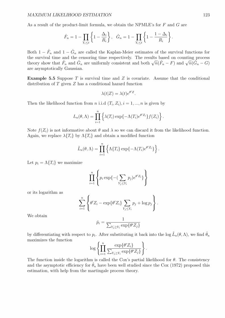
MAXIMUM LIKELIHOOD ESTIMATION 123
As a result of the product-limit formula, we obtain the NPMLE’s for F and G are
Fn = 1−∏Yi≤t
1− ∆i
Ri
, Gn = 1−
∏Yi≤t
1− 1−∆i
Ri
.
Both 1 − Fn and 1 − Gn are called the Kaplan-Meier estimates of the survival functions forthe survival time and the censoring time respectively. The results based on counting processtheory show that Fn and Gn are uniformly consistent and both
√n(Fn − F ) and
√n(Gn −G)
are asymptotically Gaussian.
Example 5.5 Suppose T is survival time and Z is covariate. Assume that the conditionaldistribution of T given Z has a conditional hazard function
λ(t|Z) = λ(t)eθ′Z .
Then the likelihood function from n i.i.d (Ti, Zi), i = 1, ..., n is given by
Ln(θ, Λ) =n∏
i=1
λ(Ti) exp−Λ(Ti)e
θ′Zif(Zi)
.
Note f(Zi) is not informative about θ and λ so we can discard it from the likelihood function.Again, we replace λTi by ΛTi and obtain a modified function
Ln(θ, Λ) =n∏
i=1
ΛTi exp−Λ(Ti)e
θ′Zi
.
Let pi = ΛTi we maximize
n∏i=1
pi exp−(
∑Yj≤Yi
pj)eθ′Zi
or its logarithm asn∑
i=1
θ′Zi − expθ′Zi
∑Yj≤Yi
pj + log pj
.
We obtain
pi =1∑
Yj≥Yiexpθ′Zj
by differentiating with respect to pi. After substituting it back into the log Ln(θ, Λ), we find θn
maximizes the function
log
n∏
i=1
expθ′Zi∑Yj≥Yi
expθ′Zj
.
The function inside the logarithm is called the Cox’s partial likelihood for θ. The consistencyand the asymptotic efficiency for θn have been well studied since the Cox (1972) proposed thisestimation, with help from the martingale process theory.
MAXIMUM LIKELIHOOD ESTIMATION 124
Example 5.6 We consider X1, ..., Xn are i.i.d F and Y1, ..., Yn are i.i.d G. We only observe(Yi, ∆i) where ∆i = I(Xi ≤ Yi) for i = 1, ..., n. This data is one type of interval censored data(or current status data). The likelihood for the observations is
n∏i=1
F (Yi)
∆i(1− F (Yi))1−∆ig(Yi)
.
To derive the NPMLE for F and G, we instead maximize
n∏i=1
P∆i
i (1− Pi)1−∆iqi
,
subject to the constraint that∑
qi = 1 and 0 ≤ Pi ≤ 1 increases with Yi. Clearly, qi = 1/n(suppose Yi are all different). This constrained maximization turns out to be solved by thefollowing steps:(i) Plot the points (i,
∑Yj≤Yi
∆j), i = 1, ..., n. This is called the cumulative sum diagram.
(ii) Form the H∗(t), the greatest the convex minorant of the cumulative sum diagram.(iii) Let Pi be the left derivative of H∗ at i.Then (P1, ..., Pn) maximizes the object function. Groeneboom and Wellner (1992) shows thatif f(t), g(t) > 0,
n1/3(Fn(t)− F (t)) →d
(F (t)(1− F (t))f(t)
2g(t)
)1/3
(2Z),
where Z is the location the maximum of the process B(t)− t2 : t ∈ R where B(t) is standardBrownian motion starting from 0.
In summary, the NPMLE is a generalization of the maximum likelihood estimation to thesemiparametric or nonparametric models. We have seen that in such a generalization, we oftenreplace the functional parameter by an empirical function with jumps only at observed dataand maximize a modified likelihood function. However, both computation of the NPMLE andthe asymptotic property of the NPMLE can be difficult and vary for different specific problems.
5.6 Alternative Efficient Estimation
Although the maximum likelihood estimation is the most popular way of obtaining an asymp-totically efficient estimator, there are alternative ways of deriving efficient estimation. Amongthem, one-step efficient estimation is the simplest.
In one-step efficient estimation, we assume that a strongly consistent estimator for parameterθ, denoted by θn, is given. Moreover |θn − θ0| = Op(n
−1/2). One-step procedure is essentially aone-step Newton-Raphson iteration in solving the likelihood score equation; that is, we define
θn = θn −
ln(θn)−1
ln(θn),
where ln(θ) is the sore function of the observed log-likelihood function and ln(θ) is the derivativeof ln(θ). The next theorem shows that θn is an asymptotically efficient estimator.
MAXIMUM LIKELIHOOD ESTIMATION 125
Theorem 5.6 Let lθ(X) be the log-likelihood function of θ. Assume that there exists a neigh-
borhood of θ0 such that in this neighborhood, |l(3)θ (X)| ≤ F (X) with E[F (X)] < ∞. Then
√n(θn − θ0) →d N(0, I(θ0)
−1),
where I(θ0) is the Fisher information. †
Proof Since θn →a.s. θ0, we perform the Taylor expansion on the right-hand side of the one-stepequation and obtain
θn = θn −
ln(θn)
ln(θ0) + ln(θ∗)(θn − θ0)
where θ∗ is between θn and θ0. Therefore,
θn − θ0 =
[I −
ln(θn)
−1
ln(θ∗)]
(θn − θ0)−
ln(θn)
ln(θ0).
On the other hand, by the condition that |l(3)θ (X)| ≤ F (X) with E[F (X)] < ∞, we know
1
nln(θ∗) →a.s. E[lθ0(X)],
1
nln(θn) →a.s. E[lθ0(X)].
Thus,
θn − θ0 = op(|θn − θ0|)−
E[lθ0(X)] + op(1)−1 1
nln(θ0)
so √n(θn − θ0) = op(1)−
E[lθ0(X)] + op(1)
−1 1√n
ln(θ0) →d N(0, I(θ0)−1).
We have proved that θn is asymptotically efficient. †
Remark 5.1 Many different conditions from Theorem 5.6 can be used to ensure the asymp-totic efficiency of θn and here we have presented a simple one. Additionally, in the one-stepestimation, since ln(θn) approximates −I(θ0) and the latter can be estimated by −I(θn), wesometimes use a slightly different one-step update:
θn = θn + I(θn)−1l(θn).
One can recognize that this estimation is in fact one-step iteration in the Fisher scoring algo-rithm. Another efficient estimation arises from the Bayesian estimation method, where it canbe shown that under regular condition of prior distribution, the posterior mode is equivalentto the maximum likelihood estimator. We will not pursue this method here.
In summary, efficient estimation is one of the most important goals in statistical inference.The maximum likelihood approach provides a natural and simple way of deriving an efficientestimator. However, when the maximum likelihood approach is not feasible, for example, themaximum likelihood estimator does not exist or the computation is difficult, other estimationapproaches may be considered such as one-step estimation, Bayesian estimation etc. So far,
MAXIMUM LIKELIHOOD ESTIMATION 126
we only focus on parametric models. When model is given semiparametrically or nonpara-metrically, the maximum likelihood estimator or the Bayesian estimator usually does not existbecause of the presence of some infinite dimensional parameters. In this case, some approxi-mated likelihood approaches have been developed, one of which is the nonparametric maximumlikelihood approach (sometimes called empirical likelihood approach) as given in Section 5.5.Other approaches include partial likelihood approach, sieve likelihood approach, and penalizedlikelihood approach etc. These topics need another full text to describe and will be deferred tosome future course.
READING MATERIALS: You should read Ferguson, Sections 16-20, Lehmann and Casella,Sections 6.2-6.7
PROBLEMS
We need the following definitions to answer the given problems.
Definition 5.2. Tn and Tn are two sequences of estimators for θ. Suppose√
n(Tn − θ) →d N(0, σ2),√
n(Tn − θ) →d N(0, σ2).
The asymptotic relative efficiency (ARE) of Tn with respect to Tn is defined as r = σ2/σ2.Intuitively, r can be understood as: to achieve the same accuracy in estimating θ, using theestimator Tn needs approximately 1/r times as many observations as using the estimator Tn.Thus, if r > 1, Tn is more efficient than Tn; vice versa.
Definition 5.3. If δ0 and δ1 are statistics, then the random interval (δ0, δ1) is called a (1−α)-confidence interval for g(θ) if
Pθ(g(θ) ∈ (δ0, δ1)) ≥ 1− α.
Intuitively, the above inequality says: however data are generated, there is at least (1 − α)probability that the interval contains the true value g(θ). Also, a random set S constructedfrom data is called a (1− α)-confidence region for g(θ) if
Pθ(g(θ) ∈ S) ≥ 1− α.
If (δ0, δ1) and S change with sample size n and the above inequalities hold at the limit, then(δ0, δ1) and S are approximately (1−α)-confidence interval and confidence region respectively.
1. Suppose that (X1, Y1),...,(Xn, Yn) are i.i.d. with bivariate normal distribution N2(µ, Σ)where µ = (µ1, µ2)
′ ∈ R2 and
Σ =
(σ2 στρστρ τ 2
)
where σ2 > 0, τ 2 > 0, and ρ ∈ (−1, 1).
MAXIMUM LIKELIHOOD ESTIMATION 127
(a) If we assume that µ1 = µ2 = θ and Σ is known, what is the maximum likelihoodestimator of θ?
(b) If we assume that µ is known and σ2 = τ 2 = θ, what is the maximum likelihoodestimator of (θ, ρ)?
(c) What is the asymptotic distribution of the estimator you found in (b)?
2. Let X1, ..., Xn be i.i.d. with common density
fθ(x) =θ
(1 + x)θ+1I(x > 0), θ > 0.
(a) Find the maximum likelihood estimator of θ, denoted as θn. Give the limit distribu-tion of
√n(θn − θ).
(b) Find a function g such that, regardless the value of θ,√
n(g(θn)− g(θ)) →d N(0, 1).
(c) Construct an approximately 1− α confidence interval based on (b).
3. Suppose X has a standard exponential distribution with density f(x) = e−xI(x > 0).Given X = x, Y has a Poisson distribution with mean λx.
(a) Determine the marginal mass function of Y . Find E[Y ] and V ar(Y ) without usingthe mass function of Y .
(b) Give a lower bound for the variance of an unbiased estimator of λ based on X andY .
(c) Suppose (X1, Y1), ..., (Xn, Yn) are i.i.d., with each pair having the same joint distri-bution as X and Y . Let λn be the maximum likelihood estimator based on thesedata, and let λn be the maximum likelihood estimator based on Y1, ..., Yn. Determinethe asymptotic relative efficiency of λn with respect to λn.
4. Suppose that X1, ..., Xn are i.i.d. with density function pθ(x), θ ∈ Θ ⊂ Rk. Denotelθ(x) = log pθ(x). Assume lθ(x) is three times differentiable with respect to θ and its thirdderivatives are bounded by M(x), where supθ Eθ[M(X)] < ∞. Let θn be the maximumlikelihood estimator of θ and assume
√n(θn − θ) →d N(0, I−1
θ ), where Iθ denotes theFisher information at θ and is assumed to be non-singular.
(a) To estimate the asymptotic variance of√
n(θn − θ), one proposes an estimator I−1n ,
where
In = − 1
n
n∑i=1
lθn(Xi).
Prove that I−1n is a consistent estimator of I−1
θ .
(b) Show √nI1/2
n (θn − θ) →d N(0, Ik×k),
where I1/2n is the square root matrix of In and Ik×k is k-by-k identity matrix. From
this approximation, construct an approximate (1− α)-confidence region for θ.
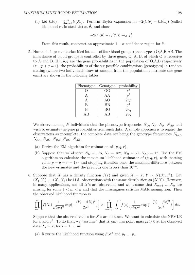
MAXIMUM LIKELIHOOD ESTIMATION 128
(c) Let ln(θ) =∑n
i=1 lθ(Xi). Perform Taylor expansion on −2(ln(θ) − ln(θn)) (called
likelihood ratio statistic) at θn and show
−2(ln(θ)− ln(θn)) →d χ2k.
From this result, construct an approximate 1− α confidence region for θ.
5. Human beings can be classified into one of four blood groups (phenotypes) O,A,B,AB. Theinheritance of blood groups is controlled by three genes, O, A, B, of which O is recessiveto A and B. If r, p, q are the gene probabilities in the population of O,A,B respectively(r + p + q = 1), the probabilities of the six possible combinations (genotypes) in randommating (where two individuals draw at random from the population contribute one geneeach) are shown in the following tables:
Phenotype Genotype probabilityO OO r2
A AA p2
A AO 2rpB BB q2
B BO 2rqAB AB 2pq
We observe among N individuals that the phenotype frequencies NO, NA, NB, NAB andwish to estimate the gene probabilities from such data. A simple approach is to regard theobservations as incomplete, the complete data set being the genotype frequencies NOO,NAA, NAO, NBB, NBO, NAB.
(a) Derive the EM algorithm for estimation of (p, q, r).
(b) Suppose that we observe NO = 176, NA = 182, NB = 60, NAB = 17. Use the EMalgorithm to calculate the maximum likelihood estimator of (p, q, r), with startingvalue p = q = r = 1/3 and stopping iteration once the maximal difference betweenthe new estimates and the previous one is less than 10−4.
6. Suppose that X has a density function f(x) and given X = x, Y ∼ N(βx, σ2). Let(X1, Y1), ..., (Xn, Yn) be i.i.d. observations with the same distribution as (X, Y ). However,in many applications, not all X’s are observable and we assume that Xm+1, ..., Xn aremissing for some 1 < m < n and that the missingness satisfies MAR assumption. Thenthe observed likelihood function is
m∏i=1
[f(Xi)
1√2πσ2
exp−(Yi − βXi)2
2σ2]×
n∏i=m+1
∫
x
[f(x)
1√2πσ2
exp−(Yi − βx)2
2σ2]
dx.
Suppose that the observed values for X’s are distinct. We want to calculate the NPMLEfor β and σ2. To do that, we “assume” that X only has point mass pi > 0 at the observeddata Xi = xi for i = 1, ...,m.
(a) Rewrite the likelihood function using β, σ2 and p1, ..., pm.

MAXIMUM LIKELIHOOD ESTIMATION 129
(b) Write out the score equations for all the parameters.
(c) A simple approach to calculate the NPMLE is to use the EM algorithm, whereXm+1, ..., Xn are missing data. Derive the EM algorithm. Hint: Xi, i = m + 1, ..., n,can only have values x1, ..., xm with probabilities p1, ..., pm.
7. Ferguson, pages 117-118, problems 1-3
8. Ferguson, pages 124-125, problems 1-7
9. Ferguson, page 131, problem 1
10. Ferguson, page 139, problems 1-4
11. Lehmann and Casella, pages 501-514, problems 3.1-7.34