REPORT

ADVANCED INTERNAL

COMBUSTION ENGINE

SENSOR ANALYSIS BY

MEANS OF MODELLING

AND REAL-TIME

MEASUREMENT

Heime Jonkers

EWI DATAMANAGEMENT & BIOMETRICS EXAMINATION COMMITTEE

Prof.Dr.Ir. R.N.J.Veldhuis, dr. G.G.M. Stoffels, dr. ir. A.J. Annema

DOCUMENT NUMBER

EWI19/DMB - BA-EE/001/HJ

24-01-2019

Abstract Given modern increased ability to model, measure and process the operation conditions of the internal combustion engine, an opportunity was presented to greatly improve the performance of older combustion engines through the development of a more affordable engine management system. As part of the development of this system, a study into the possible improvements to the usage of common automotive drivetrain sensors was conducted, resulting in a numerical model of the common SI (Spark Ignition) engine, the development of a real time measurement system and a set of real-time measurements on a representative Volvo b230k engine. These real time measurements were combined with the created model to result in the finding of 3 additional uses for the common MAP (Manifold Air Pressure) sensor, namely engine speed determination, crank angle position read out and camshaft profile identification. Additionally, methodologies for the usage of EGT (Exhaust Gas Temperature) sensors for the determination of the AFR (Air Fuel ratio) with provided engine speed were proposed, and the possible relationship between MAT (Manifold Air Temperature) and engine operating friction were discussed.

Preface The subject of this research was based in my personal interest in the motorcycle and car hobby, and my future ambitions to start a company specialized in the improvement of the performance of the vehicles commonly used in this hobby. This project has allowed me to gain a lot of knowledge on the topic of engine management, tuning and the creation of engine control systems, which will most definitely be applied in future projects and the development of my company. I would like to thank my examiners and supervisors Prof.Dr.Ir. R.N.J. Veldhuis, dr.ir. A.J. Annema and dr. G.G.M. Stoffels as well as my unofficial supervisor ing. G.J. Laanstra for their much-appreciated help and contribution during the weekly and individual meetings as well as for their helpful suggestions during project roadblocks. I additionally would like to thank my family and friends for their help and understanding during the key moments of this project, and their key advice during the finishing stages of this project.

1

Contents Contents ....................................................................................................................................................................1

Introduction ...............................................................................................................................................................2

The IC Engine: Theory ................................................................................................................................................3

A brief history of the internal combustion engine ..................................................................................................3

Operating principles of the internal combustion engine ........................................................................................3

The Two and Four stroke engine ............................................................................................................................4

The Diesel and Otto cycle.......................................................................................................................................6

Description of proposed test engine ......................................................................................................................8

The IC Engine: Modelling ..........................................................................................................................................10

Modelling research ..............................................................................................................................................10

Model construction .............................................................................................................................................11

Parameters from model .......................................................................................................................................17

The IC Engine: Real-Time Measurement ...................................................................................................................19

Sensors ................................................................................................................................................................19

Sensor placement ................................................................................................................................................20

Measurement ......................................................................................................................................................21

Method................................................................................................................................................................22

Discussion ............................................................................................................................................................22

Operating Conditions: Theory vs Practice .................................................................................................................24

Manifold Air Pressure ..........................................................................................................................................24

Manifold Air Temperature ...................................................................................................................................26

Exhaust Gas Temperature ....................................................................................................................................27

Operating Conditions: Extraction .............................................................................................................................29

Engine speed .......................................................................................................................................................29

Engine rotation ....................................................................................................................................................30

Camshaft profile. .................................................................................................................................................30

Engine fueling and load ........................................................................................................................................31

Concluding ...............................................................................................................................................................32

Achievements ......................................................................................................................................................32

Thesis discussion..................................................................................................................................................32

Suggested additional development ......................................................................................................................32

2

Introduction In the car and motorcycle hobby, wherein the maintenance, driving/riding and improvement of old vehicles is often the motivation, the demand for better fuel economy, control, power and reliability are requested[1.7], [1.8]. A cost-effective solution to these demands is often found in an electronic fuel injection (EFI) and electronic ignition (EI)

conversion, which replaces the often dated original and often mechanical fuel and ignition system by a more precisely controllable electronic system[1.9], [1.10]. The added control offered by these systems also allows for improved emission performance at the cost of system simplicity[1.11],[1.12].

Great opportunity Given modern improvements in the ability to process[1.1], model[1.2] and measure[1.3],[1.4] the operating conditions of the internal combustion engine, an opportunity is presented to greatly improve the performance of older combustion engine powered hobbyist cars and motorcycles. Which is of the essence amongst ever more stringent emission demands[1.5] to allow for the longer survival of the hobby, amongst a world switching to the electric motor vehicle[1.6]. These conversions are however often found to be inaccessible for most hobbyist due to the complex calibration

and often substantial costs of these systems[1.11] in comparison to the original system. An issue which was proposed

to be addressed by the development of a more affordable and simple electronic fuel injection and ignition system

by retaining only the most necessary of functions and sensors, simplifying calibration and reducing system

complexity.

Road to progress During this report the initial step towards such a system will be discussed through means of an advanced analysis of

the system to be controlled. Starting off with research towards common combustion engine operation principles,

from which a numeric combustion engine model in the MATLAB environment will be created. This model will then

be used along with the research into common engine operating principles to distill the key measurable quantities

for the determination of the engine’s running condition.

With the key measurements determined, an advanced analysis into the capabilities of the currently available

internal combustion engine sensors shall be performed based upon ranking in speed, prevalence and accuracy. This

analysis is then be followed by a series of real-time measurements with the top ranked sensors on a combustion

engine as is representative of those favored the car and motorcycle hobbyist, including a description of the

measurement system and processing algorithm.

This initial step shall be followed by a validation of the expected extractable operating parameters per sensor, based in comparison of combustion engine operating theory, the performed measurements and the results from the numerical model. This validation will then be followed by the suggestion of a method for the consistent detection and measurement of these key engine operation indicators.

Quantification of results

A summary of the attained improvements will then be discussed in an attempt to prove the below stated thesis: “Given the modern processing, modelling and measurement capabilities, a reduction of sensors used and additional control for internal combustion engine management can be achieved through the extraction of multiple key engine operating parameters from a single sensor”

3

The IC Engine: Theory Starting of the research the operating principles of the engine to be modelled and measured upon would have to be determined, in this chapter a summary of the obtained theory and a detailed description of the operation of the engine to be tested upon will be provided.

A brief history of the internal combustion engine In order to get a better understanding of the operating principles and theory behind the internal combustion engine. We will start off with a brief history of the internal combustion engine, focused on the intermittent-combustion based engine developments that eventually led to the engines used in automotive sector. In 1794, Robert Street developed a device which used gas expansion to move a piston which in turn moved a water pump as a form of work[2.1], displaying the principle of the usage of internal combustion as an engine. In 1807 the concept of the internal combustion engine in a transport vehicle was shown by Nicéphore Niépce who managed to create a boat, propelled by a pulse propulsion system based on expansion, used to displace water in order to create movement[2.2]. After several more years of development, in 1860 Étienne Lenoir managed to create the first practical gas expansion engine, with relatively modern operation, and comparably economical to the steam engine[2.1]. Another improvement to the operation of the combustion engine came with the 4-stroke engine cycle as patented in 1876 by Nikolaus Otto, which improved engine efficiency and added control by introducing an introduced spark to control ignition[2.3]. The 4-stroke, Otto-cycle engine was also adapted in the first production automobile created by Carl Benz in 1885[2.4]. Twelve years later in 1897 Rudolf Diesel presented the Diesel compression ignition engine, with very high efficiency for the time period[2.5]. A combination of the Otto-cycle (carbureted) and Diesel-cycle engine was also developed in 1925, which was able to burn heavy fuels at low compression with efficiency figures somewhere in between the two engines it combined[2.6]. Later developments were mostly based in the optimization of existing engine cycles and designs, with NSU developing the Wankel piston less engine in 1954[2.7], Daimler-Benz claiming a patent for the scotch yoke engine in 1986[2.8]. More recently with increasing emission demands, new cycle strategies have been developed to increase engine efficiency even further as shown by Mazda with their HCCI (Homogeneous Charge Compression Ignition) engine innovation in 2017[2.9].

Operating principles of the internal combustion engine As was already addressed in less detail above, the internal combustion engine is a system wherein an oxidizer and fuel are combined to create an explosion or combustion, to perform work in the engine. Through the combustion of the working fluids (oxidizer and fuel) heat is generated and transferred to the products of combustion, which are often hot gasses, that act upon for example a moving piston, blade or the outside environment in the case of a nozzle[2.10]. For the explanation of the operating principles we will focus on the reciprocating engine, since these are most commonly found in ground transportation applications. For these intermittent combustion engine where combustion occurs on cyclic occasions, and discrete quantities of the working fluids are processed during each cycle in a specific set of steps[2.10].

4

The Two and Four stroke engine To start the explanation these cycles, we have to define the steps which occur during the cycle, reciprocating engine designs can commonly be divided into 2-stroke, 4-stroke designs, which will be explained below. However, a general description of the piston crank mechanism as shown in figure 2.1 is first in order. As can be observed in the picture, the piston crank mechanism consists of a crank as shown at the bottom of the picture, a rod connecting the piston and the crankshaft, and a piston(1) moving in a cylinder(2), enclosed at the top to form a chamber, wherein depending on the engine design valves and a spark inducer are included. As the crank rotates the chamber volume is increased as the stroke of the crank is swept by the piston, when the piston is at its highest point as the crank is rotated this is called Top Dead Center (TDC), the lowest point that the piston reaches during the rotation is called the Bottom Dead Center (BDC)[2.11].

The four-stroke engine We will start off with the 4-stroke, since this is the most common and easiest to explain. The 4-stroke cycle can be described in 4 consecutive steps in order as shown in figure 2.2:

Figure 2.2 – 4 stroke engine cycles[2.F2]

1. Induction During the induction phase of the cycle, the piston moves downwards from TDC to BDC whilst the inlet valve is

opened, the fuel and oxidizer mixture with a fuel to oxidizer ratio often defined as the air-fuel ratio (AFR) in the

case air is used as the oxidizer, the derivation from[2.12], is sucked in as the chamber volume increases and therefore

results in a vacuum to be filled. The amount of mixture volume drawn in compared to the actual chamber volume

reached at BDC, is called the Volumetric Efficiency (VE)[2.13].

2. Compression During the compression phase of the cycle, both valves are closed, as the piston moves upwards from BDC to TDC,

compressing the mixture to increase engine efficiency[2.14]. The mixture is compressed by the compression ratio,

specified by the BDC chamber volume divided by the TDC chamber volume[2.14].

Figure 2.1 – Line art drawing of a piston-cylinder-crank system[2.F1], with a spark plug and valves also shown for the combustion chamber

5

3. Combustion

During the combustion phase of the cycle, the mixture is ignited through either a spark in the case of a spark

ignition (SI)[2.15] engine, or through the compression itself in the case of a compression ignition (CI) [2.15] engine. The

mixture combusts and drives the piston down from TDC to BDC, to drive the crankshaft.

4. Exhaust

During the exhaust phase of the cycle, the exhaust valve opens as the piston moves from BDC to TDC, and the

combustion products exit the chamber, first quickly during the blowdown stage due to the residual pressure in the

chamber, followed by the exhaust displacement where the residual combustion products are mostly

evacuated[2.16].

The two-stroke engine The next configuration to discuss is the 2-stroke, which simplifies the 4-stroke engine into a less complex valve less

design. The 2-stroke also has the benefit of being able to deliver power every engine rotation since the combustion

occurs on every crank rotation. This allows for lighter and more compact engine design of the power with a

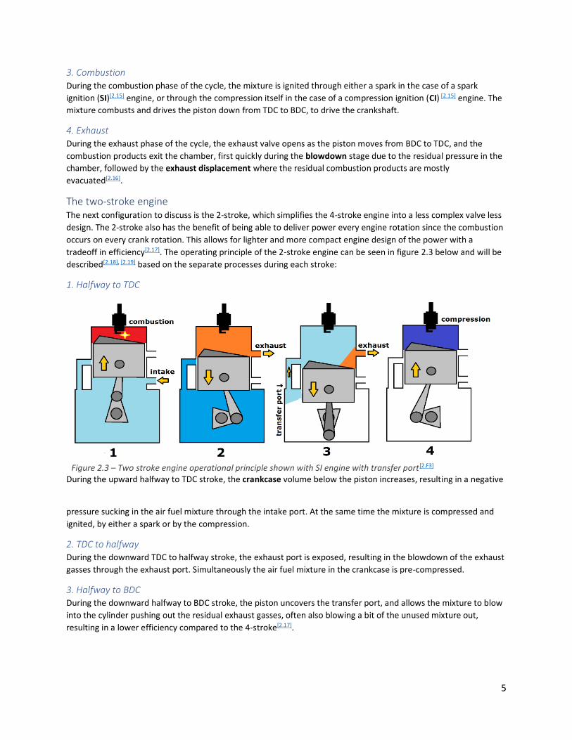
tradeoff in efficiency[2.17]. The operating principle of the 2-stroke engine can be seen in figure 2.3 below and will be

described[2.18], [2.19] based on the separate processes during each stroke:

1. Halfway to TDC

During the upward halfway to TDC stroke, the crankcase volume below the piston increases, resulting in a negative

pressure sucking in the air fuel mixture through the intake port. At the same time the mixture is compressed and

ignited, by either a spark or by the compression.

2. TDC to halfway During the downward TDC to halfway stroke, the exhaust port is exposed, resulting in the blowdown of the exhaust

gasses through the exhaust port. Simultaneously the air fuel mixture in the crankcase is pre-compressed.

3. Halfway to BDC During the downward halfway to BDC stroke, the piston uncovers the transfer port, and allows the mixture to blow

into the cylinder pushing out the residual exhaust gasses, often also blowing a bit of the unused mixture out,

resulting in a lower efficiency compared to the 4-stroke[2.17].

Figure 2.3 – Two stroke engine operational principle shown with SI engine with transfer port[2.F3]

6

4. BDC to halfway

During the upward BDC to halfway stroke, the combustion mixture is compressed in preparation for combustion. The exhaust displacement is left from the model, since per air standard assumption, it will return to the exact same state after the induction.

The Diesel and Otto cycle With the basic operation of the two- and four-stroke engine operation discussed, a more detailed look at the most

commonly used thermodynamic cycles for spark and compression ignition engines. The Otto and the Diesel Cycle.

To be able to simplify the analysis of both cycles we will first define the air-standard assumptions[2.20]: 1. “The working fluid is air, which continuously circulates in a closed loop and always behaves as an ideal gas” 2. “All the processes that make up the cycle are internally reversible” 3. “The combustion process is replaced by a heat-addition process from an external source” 4. “The exhaust process is replaced by a heat-rejection process that restores the working fluid to its initial

state”

The Otto Cycle[2.20] The Otto cycle, as invented by Nikolaus Otto[2.3] can quite easily be modelled with the use of the air standard assumptions. A 4-stroke engine will be assumed, to serve as guide for the explanation of each process as shown in figure 2.4.

Induction – Process 1: The induction process is not modelled since it is assumed according to the standard air assumptions that the same fluid remains in the closed loop. This can be interpreted as that the intake cycle is assumed to take in exactly the correct amount of air each cycle, and that this condition is the same as the chamber condition after all of the added energy from the combustion is removed.

Compression – Process 1 -> 2: The compression phase is modelled as an Isentropic compression process[2.20], for which it can be said that during the compression process work is transferred without friction and no transfer of heat or matter will occur.

Combustion – Process 2 -> 3 -> 4:

The combustion of the mixture is modelled as a constant volume addition of heat. This also defines that the fuel mixture for spark ignition engines has to burn quickly after the spark plug ignites the mixture for this statement to hold. The piston being driven down then is modelled as Isentropic expansion.

Exhaust – Process 4 -> 1: The exhaust process is modelled through constant volume heat rejection, modelling the rapid blowdown of the

chamber as the exhaust valve opens, removing the added combustion energy. The exhaust displacement is left

from the model, since per air standard assumption, it will return to the exact same state after the induction.

Figure 2.4 – Pressure/Volume diagram for the Otto cycle[2.F4]

7

The Diesel Cycle[2.20] The Diesel Cycle as invented by Rudolf Diesel[2.5] can also be easily modelled with the use of the air standard assumptions. As with the Otto cycle a 4-stroke engine will be assumed for the description of the model, as shown in figure 2.5.

Induction – Process 1: The induction process is once more left out of the model since it is assumed according to the standard air assumptions that the same fluid remains in the closed loop. This can be interpreted as that the intake cycle is assumed to take in exactly the correct amount of air each cycle, and that this condition is the same as the chamber condition after all of the added energy from the combustion is removed.

Compression – Process 1 -> 2:

The compression process is modelled as Isentropic

compression once more, meaning that all work will be

transferred without loss and no mass or heat is transferred.

Combustion – Process 2 -> 3 -> 4:

The combustion is the point where the Otto and Diesel cycle differ, for the Diesel it is assumed that the fuel will

burn slowly at a constant pressure after the pressure required for ignition is reached, as represented in the P-V

diagram. It is therefore modelled as constant pressure heat addition. In reality ignition is achieved by injecting fuel

at the somewhere around TDC where peak pressure occurs. The piston being driven down is modelled once more

as Isentropic expansion.

Exhaust – Process 4 -> 1:

The exhaust blowdown process is modelled once more as a heat rejection at constant volume, returning to the

condition assumed at the end of the induction process, as all of the added heat is removed.

Comparative efficiencies[2.20]

In order to be able to give some reference for the relative efficiencies of these two cycles, the thermal efficiencies can be determined for the Otto and Diesel cycle as shown below in equations 2.1a and 2.1b.

𝜂𝑡ℎ,𝑂𝑡𝑡𝑜 = 1 −1

𝑟𝑘−1𝑤𝑖𝑡ℎ

𝑟: 𝑐𝑜𝑚𝑝𝑟𝑒𝑠𝑠𝑖𝑜𝑛 𝑟𝑎𝑡𝑖𝑜

𝑘: 𝑠𝑝𝑒𝑐𝑖𝑓𝑖𝑐 ℎ𝑒𝑎𝑡 𝑟𝑎𝑡𝑖𝑜𝐶𝑝

𝐶𝑣

𝜂𝑡ℎ,𝐷𝑖𝑒𝑠𝑒𝑙 = 1 −1

𝑟𝑘−1[

𝑟𝑐𝑘−1

𝑘(𝑟𝑐−1)𝑤𝑖𝑡ℎ

𝑟: 𝑐𝑜𝑚𝑝𝑟𝑒𝑠𝑠𝑖𝑜𝑛 𝑟𝑎𝑡𝑖𝑜 𝑟𝑐: 𝑐𝑢𝑡𝑜𝑓𝑓 𝑟𝑎𝑡𝑖𝑜

𝑘: 𝑠𝑝𝑒𝑐𝑖𝑓𝑖𝑐 ℎ𝑒𝑎𝑡 𝑟𝑎𝑡𝑖𝑜𝐶𝑝

𝐶𝑣

Equation 2.1a – Thermal efficiency of Otto Cycle Equation 2.1b – Thermal efficiency of Diesel Cycle Given that the specific heat ratio for air is k = 1.4 for air at room temperature, and given that the cutoff ratio representative of the chamber after and before the combustion event is always greater than 1 for a compression ignition engine, it can be shown that 𝜂𝑡ℎ,𝑂𝑡𝑡𝑜 > 𝜂𝑡ℎ,𝐷𝑖𝑒𝑠𝑒𝑙 given equal compression ratio r.

However, spark ignition engines suffer from autoignition, which is the pre-ignition of the fuel-air mixture due to the compression of the mixture, which results in engine knock an audible noise, damage to the engine and efficiency loss. The compression ignition engine does not suffer this issue since only air is compressed after which fuel is later introduced, allowing for higher compression ratios for diesel cycle engines when compared to Otto cycle engines. From this and several additional real-world constraints not discussed, practical efficiencies of 25-30% can be achieved for the Otto cycle, and practical efficiencies of 35-40% are observed for the Diesel cycle.

Figure 2.5 – Pressure/Volume diagram for the Diesel cycle[2.F5]

8

Description of proposed test engine Since the most common engine found in automotive application is the four-stroke, gasoline-powered,

homogeneous charge spark ignition engine[2.10] operating on the Otto-cycle. To allow for appropriate modelling and

measurements on an engine of this category, an available Volvo B230K engine was chosen, a 4-Stroke spark ignition

petrol engine representative of the common hobbyist produced in 1986, for which the specifications are listed in

table 2.1 below.

Property Specification Brief explanation

Displacement 2316 [𝑐𝑚3] The displacement is the amount of displaced (air) volume for each complete engine cycle and can be determined from the chamber volume change for a single cycle.

Configuration In-line 4 The configuration determines the manner wherein the multiple pistons of a multiple piston engine move in comparison to one another

Firing order 1-3-4-2 The firing order determine in which order combustion will occur in each cylinder of the engine

Stroke 80.0 [mm] The stroke is the length of horizontal movement by the piston

Bore 96.0 [mm] The bore is the diameter of the cylinder in which the piston moves

Compression ratio 10.3 The compression ratio is the ratio of the chamber volume with the piston at TDC vs the chamber volume with the piston at BDC

Cylinder head configuration

2 valves per cylinder, with overhead camshaft

The valves per cylinder allow for a specification of chamber configuration and an estimate of maximum volumetric efficiency, since only so much of the total bore surface can be covered by valves due to design constraints for the valves.

Valve size In: 44Ø [mm] Ex: 35Ø [mm]

The valve diameters are an important factor in estimating the airflow into and out of the engine

Camshaft specification

Volvo k-profile: Lift in, out: 11.95 [mm] LSA: 110° Duration in: 270° Duration ex: 257°

The engine had a Volvo k-profile camshaft installed for a different performance

characteristic, found under the name of KG004 in [2.23]. The lift determines the

opening of the valves, the LSA the spacing of opening moments between the intake and exhaust valve, and the duration determines how long the valves are open.

Fuel and ignition Fuel: Bosch LH2.4 fuel injection from b230f engine Ignition: Bosch EZK116 from b230f engine

The engine was converted from carburetor to a fuel injection system from a more modern Volvo b230f engine. The system used contained an air fuel ratio and detonation sensor to allow for smooth fuel delivery and correct timing of the ignition events.

Table 2.1 – Specifications of modelled b230k engine [2.21], [2.22], [2.23], [2.24], [2.25]

Since these specifications might allow for confusion without proper description and a visual representation figure

2.6 below was created from previous teardown experience with these engines as well as with the use of the Haynes

Manual[2.26].

Mechanical operation The engine’s operation can be described as follows from the figure, the camshaft(1) pushes on the valve springs(2)

covered by a bucket (a metal cup, to allow for a more wear proof interaction between the cam and the springs),

resulting in the exhaust(9) and intake(8) valves to be pushed opened from the normally closed position. The

camshaft(1) is driven by the timing belt and gears(10) maintaining a rotation relation of 2:1 between camshaft and

the crankshaft, meaning 2 crankshaft(5) rotations equal one rotation of the camshaft(1), since for one cycle of the 4-

stroke engine for a single cylinder the intake and exhaust valve are only pushed open once as shown in figure 2.2.

Both the camshaft(1) and crankshaft(5) are supported by bearing surfaces lubricated by oil to ensure minimal friction.

Attached to the crankshaft(5) are the connecting rods(6) via another bearing surface to which the pistons P1-P4 are

attached through means of a pin and bearing surface, in which rings can also be observed sealing the piston to the

cylinder walls they are contained within as shown in figure 2.1.

9

The camshaft(1) has lobes as shown in the camshaft closeup, which determine the profile and timing of the valve

openings, with the base circle(C2) the section of the lobe where the springs are not pushed down, lift(C1) the amount

in [mm] the valves are pushed down and the duration(C3), the amount of rotation for which the springs and valves

are pushed down and the lobe is higher than the base circle.

Thermal operation In the figure the coolant passages(4) can also be observed in the Aluminum cylinder head as well as in the cast steel block[2.22], which serve to keep the engine temperature equal and allow for the liquid cooling of the system, to get rid of residual heat caused by heat transfer through the chamber walls and intake and exhaust ports. Figure 2.6 also shows the Otto cycle steps, as is correct for the Volvo engine’s firing order of P1 -> P3 -> P2 -> P4 -> P2 [2.22]. With P1 at the end of the induction process, with the intake valve(8) open, the exhaust(9) closed and the chamber filled with uncompressed air-fuel mixture. P2 can be observed to be at TDC during ignition with both valves closed, and a compressed mixture in the camber. P4 is shown at BDC after the expansion of the combusted mixture, with both valves still closed. P3 is shown with the piston at TDC after the blowdown and displacement of the exhaust gasses, with the exhaust valve opened. It can also be observed that the camshaft lobes are configured in such a manner that for every half rotation of the crankshaft a combustion event can occur in each cylinder.

Additional notes Some additional notes are to be considered for the used test engine, starting off with the note that the used engine had a mileage of approximately 0.55 million kilometers was well maintained and remained in good condition, as confirmed by a cranking compression measurement as described in the Haynes manual[2.26] It is also to be mentioned that the engine had improved intake and exhaust systems installed, which are assumed to have reduced airflow restriction in the air path to and from the chambers.

Figure 2.6 – Cut through illustration of Volvo B230 engine[2.F6]

10

The IC Engine: Modelling With the now determined properties and operating principles of a for hobbyist’s representative internal combustion engine, a model can be created to closely represent the engine’s thermal and mechanical behavior, in order to asses relevant measurable operation parameters. The proposed model was created in the MATLAB[3.1] environment and based upon an improved model of the Otto-cycle estimate with the use of the air-standard assumptions, with inclusion of valve, plenum and temperature dependent air density models.

Modelling research At the start of the model creation, a look was had into previously discovered resources as part of pre-research into

the creation of an electronic fuel injection and ignition system, which was divided into several categories of which

Appendix A1 concerned internal combustion engine modelling. In summary [A1.1, A1.4] described a discussion of open

and closed loop control modelling less relevant to the created model, [A1.5] described the creation of a Simulink[3.1]

model of an engine management system, which would be more relevant to the sensor selection described in the

measurement chapter. Resource [A1.3] was disqualified since it was written in Chinese with only an English abstract

and concluding [A1.2] described the most relevant modelling of combustion chamber conditions for NO2x prediction

in MATLAB[3.1], from which the usage pressure-volume modelling and the usage of crankshaft rotation as timescale

was noted.

Due to the somewhat insufficient information determined from the pre-research, additional information was

sourced through Khan Academy[3.2a-f] concerning the topic of thermodynamics, with in specific details on specific

heat, internal energy/work, piston problems and engine’s and their efficiency. After discussion with several

Mechanical Engineering students, a version of ‘Thermodynamics: An Engineering approach[3.3]’ was attained in

order to get more information on Otto-cycle modelling and a better understanding of energy/work relationships.

Commonly applied model and improvements From the previously discussed resources, it was concluded that the most common model, applicable to the desired results would be the Otto-Cycle model with the usage of the air-standard assumption, as proposed and described in the combustion engine operating principles chapter attained from[3.3]. In order to get a more accurate model, some of the assumptions made in this model were reconsidered. Firstly, the assumption that the exhaust and intake stroke can be left out is reconsidered, since this assumption requires for identical chamber conditions at the beginning of the exhaust displacement and the end of the intake stroked. This is inaccurate since the intake stroke almost never allows for complete chamber filling (Volumetric Efficiency) due to restrictions in the intake path determined partly by the valve size and opening[3.4]. It should additionally be considered that the exhaust evacuation is also dependent upon engine speed and camshaft profile, allowing for further inaccuracies[3.5]. Secondly the assumption of constant specific heat is inaccurate, since for air the specific heat is dependent upon temperature[3.6], which shall be tackled through the implementation of recalculation of specific heat for each simulation step. Thirdly, improvements could be made by replacing the working fluid by the actual mixture and converting this fluid to the gasses resulting from combustion along with the residual mixture. However, the implementation of this proposal was left from the model, since the formed combustion products are temperature and fuel timing dependent[A1.2] and thus difficult to estimate, and since the additional calculation for the multiple gasses would add a great amount of model complexity.

11

Model construction With the above described improvements, the adapted Otto-cycle model was based in the following assumptions.

1. The working fluid is dry air, that behaves as an ideal gas. 2. The air in the piston chambers and plenum remains in quasi-equilibrium 3. The combustion process is replaced by a heat addition through the energy release of all of the energy

available in the provided fuel. 4. All airflow through the valves shall be choked in flow. 5. No heat transfer shall occur between system components, except through the energy contained in the air

mass passed through the valves.

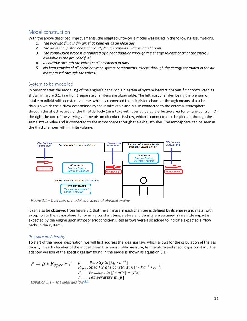
System to be modelled In order to start the modelling of the engine’s behavior, a diagram of system interactions was first constructed as

shown in figure 3.1, in which 3 separate chambers are observable. The leftmost chamber being the plenum or

intake manifold with constant volume, which is connected to each piston chamber through means of a tube

through which the airflow determined by the intake valve and is also connected to the external atmosphere

through the affective area of the throttle body (air intake with user adjustable effective area for engine control). On

the right the one of the varying volume piston chambers is show, which is connected to the plenum through the

same intake valve and is connected to the atmosphere through the exhaust valve. The atmosphere can be seen as

the third chamber with infinite volume.

Figure 3.1 – Overview of model equivalent of physical engine

It can also be observed from figure 3.1 that the air mass in each chamber is defined by its energy and mass, with exception to the atmosphere, for which a constant temperature and density are assumed, since little impact is expected by the engine upon atmospheric conditions. Red arrows were also added to indicate expected airflow paths in the system.

Pressure and density To start of the model description, we will first address the ideal gas law, which allows for the calculation of the gas density in each chamber of the model, given the measurable pressure, temperature and specific gas constant. The adapted version of the specific gas law found in the model is shown as equation 3.1.

𝑃 = 𝜌 ∗ 𝑅𝑠𝑝𝑒𝑐 ∗ 𝑇 𝜌: 𝐷𝑒𝑛𝑠𝑖𝑡𝑦 𝑖𝑛 [𝑘𝑔 ∗ 𝑚−3] 𝑅𝑠𝑝𝑒𝑐: 𝑆𝑝𝑒𝑐𝑖𝑓𝑖𝑐 𝑔𝑎𝑠 𝑐𝑜𝑛𝑠𝑡𝑎𝑛𝑡 𝑖𝑛 [𝐽 ∗ 𝑘𝑔−1 ∗ 𝐾−1] 𝑃: 𝑃𝑟𝑒𝑠𝑠𝑢𝑟𝑒 𝑖𝑛 [𝐽 ∗ 𝑚−3] = [𝑃𝑎] 𝑇: 𝑇𝑒𝑚𝑝𝑒𝑟𝑎𝑡𝑢𝑟𝑒 𝑖𝑛 [𝐾]

Equation 3.1 – The ideal gas law[3.7]

12

The next relevant equation is the calculation of the density, as shown below in Equation 3.2, which is used to relate chamber mass and volume and is later required for the flow calculations. This is also why the quasi-equilibrium assumption is required, since without an even distribution of gas particles, it cannot be assumed that the density at the valves is well represented by the mass in the chamber compared to the chamber volume.

𝜌 =𝑚

𝑉

𝜌: 𝐷𝑒𝑛𝑠𝑖𝑡𝑦 𝑖𝑛 [𝑘𝑔 ∗ 𝑚−3] 𝑚: 𝑀𝑎𝑠𝑠 𝑜𝑓 𝑔𝑎𝑠 𝑖𝑛 [𝑘𝑔] 𝑉: 𝑉𝑜𝑙𝑢𝑚𝑒 𝑖𝑛 [𝑚3]

Equation 3.2 - Density[3.9]

Energy

The third defining equation for the model is the relation of changing the gas masses temperature to its internal energy, allowing for a method of determining the added energy through combustion, as well as the energy contained in the gas in each chamber relative to a starting temperature. This equation will be used for both the combustion model as the flow model, where heat addition and rejection to the chamber masses occurs. The equation can be found as Equation 3.3 and was defined for constant volume heat rejection and addition, since combustion for an SI engine occurs with constant volume, and since it is assumed that the valve flow and thus chamber energy loss and addition calculations occur for relatively constant piston volume, if the chosen simulation resolution is high. This will further be explained during the detailed description of these models.

∆𝑄 = 𝑐𝑣 ∗ 𝑚 ∗ ∆𝑇 𝑄: 𝐸𝑛𝑒𝑟𝑔𝑦 𝑖𝑛 [𝐽] 𝑐𝑣: 𝐻𝑒𝑎𝑡 𝑐𝑎𝑝𝑎𝑐𝑖𝑡𝑦 𝑓𝑜𝑟 𝑐𝑜𝑛𝑠𝑡𝑎𝑛𝑡 𝑣𝑜𝑙𝑢𝑚𝑒 𝑖𝑛 [𝐽 ∗ 𝑘𝑔−1 ∗ 𝐾−1] 𝑚: 𝑀𝑎𝑠𝑠 𝑜𝑓 𝑔𝑎𝑠 𝑖𝑛 [𝑘𝑔] 𝑇: 𝑇𝑒𝑚𝑝𝑒𝑟𝑎𝑡𝑢𝑟𝑒 𝑖𝑛 [𝐾]

Equation 3.3 – Heat capacity per unit mass provided a constant volume[3.8]

As discussed previously in the section on suggested model improvements, the model shall use a more accurate calculation of 𝑐𝑣, that includes a temperature dependence, which was calculated through the use of Equation 3.4a of which the curve fit is discussed further in appendix E1.

𝑐𝑣 = −9.000 ∗ 10−9𝑇2 + 2.000 ∗ 10−4𝑇 + 0.6512 𝑇: 𝑇𝑒𝑚𝑝𝑒𝑟𝑎𝑡𝑢𝑟𝑒 𝑖𝑛 [𝐾] Equation 3.4a – Estimate equation of specific heat for constant volume [E1]

Expansion and compression model In order to determine the expansion and compression within the piston chamber, a calculation of the volume of the

chamber for each degree of crankshaft rotation was required. To achieve this piston displacement model was

adapted, to calculate crankshaft rotation dependent piston height referenced to piston BDC as shown in Equation

3.5, which could then be subtracted from the stoke and multiplied by the piston’s surface area, to calculate the

stroked volume. With the stroked volume and TDC chamber volume known, the complete piston chamber volume

was defined.

𝑠(𝜃) =𝑆𝑡𝑟𝑜𝑘𝑒

2cos(𝜃) + √𝐿𝑐𝑜𝑛𝑛𝑒𝑐𝑡2 − (

𝑆𝑡𝑟𝑜𝑘𝑒

2∗ sin(𝜃))

2

𝑠(𝜃): 𝑣𝑒𝑟𝑡𝑖𝑐𝑎𝑙 𝑝𝑖𝑠𝑡𝑜𝑛 𝑑𝑖𝑠𝑝𝑙𝑎𝑐𝑒𝑚𝑒𝑛𝑡 𝑟𝑒𝑓𝑒𝑟𝑒𝑛𝑐𝑒𝑑 𝑡𝑜 𝑐𝑟𝑎𝑛𝑘𝑠ℎ𝑎𝑓𝑡 𝑐𝑒𝑛𝑡𝑒𝑟𝑙𝑖𝑛𝑒 𝑖𝑛 [𝑚]

𝑦(𝜃) = 𝑠(𝜃) +𝑆𝑡𝑟𝑜𝑘𝑒

2− 𝐿𝑐𝑜𝑛𝑛𝑒𝑐𝑡 𝑦(𝜃): 𝑣𝑒𝑟𝑡𝑖𝑐𝑎𝑙 𝑑𝑖𝑠𝑝𝑙𝑎𝑐𝑒𝑚𝑒𝑛𝑡 𝑜𝑓 𝑝𝑖𝑠𝑡𝑜𝑛

𝑟𝑒𝑓𝑒𝑟𝑒𝑛𝑐𝑒𝑑 𝑡𝑜 𝑝𝑖𝑠𝑡𝑜𝑛 𝐵𝐷𝐶 𝑖𝑛 [𝑚] 𝜃: 𝑎𝑛𝑔𝑙𝑒 𝑜𝑓 𝑐𝑟𝑎𝑛𝑘𝑠ℎ𝑎𝑓𝑡 𝑟𝑜𝑡𝑎𝑡𝑖𝑜𝑛 𝑖𝑛 [𝑟𝑎𝑑] 𝑆𝑡𝑟𝑜𝑘𝑒: 𝑠𝑡𝑟𝑜𝑘𝑒 𝑜𝑓 𝑐𝑟𝑎𝑛𝑘𝑠ℎ𝑎𝑓𝑡 𝑖𝑛 [𝑚] 𝐿𝑐𝑜𝑛𝑛𝑒𝑐𝑡: 𝑙𝑒𝑛𝑔ℎ𝑡 𝑜𝑓 𝑐𝑜𝑛𝑛𝑒𝑐𝑡𝑖𝑛𝑔 𝑟𝑜𝑑 𝑖𝑛 [𝑚]

Equation 3.5 - Piston displacement[3.10]

13

With the new chamber volume now determined, Equation 3.6 for the Isentropic compression and expansion could then be applied with the use of the specific heat ration 𝛾 as calculated with the use of Equation 3.4b, given the previous and current chamber volume, to determine the temperature within the piston chamber.

𝛾 = −2.000 ∗ 10−8𝑇2 − 4.000 ∗ 10−6𝑇 + 1.405 𝑇: 𝑇𝑒𝑚𝑝𝑒𝑟𝑎𝑡𝑢𝑟𝑒 𝑖𝑛 [𝐾]

Equation 3.4b – Estimate equation of specific heat ratio [E2]

𝑇2

𝑇1= (

𝑉1

𝑉2)

𝛾−1

𝑇: 𝑇𝑒𝑚𝑝𝑒𝑟𝑎𝑡𝑢𝑟𝑒 𝑖𝑛 [𝐾] 𝑉: 𝑉𝑜𝑙𝑢𝑚𝑒 𝑖𝑛 [𝑚3] 𝛾: 𝑆𝑝𝑒𝑐𝑖𝑓𝑖𝑐 ℎ𝑒𝑎𝑡 𝑟𝑎𝑡𝑖𝑜

Equation 3.6 -Temperature and Volume relation for Isentropic process[3.11] After the application of Equation 3.6 the model recalculates the chamber pressure based upon Equation 3.1 and 3.2, the chamber conditions were initialized at BDC, assuming the intake stroke had just occurred and filled the camber completely with air at a temperature of 20 [℃] and a pressure equal to the standard atmospheric pressure of 101 [𝑃𝑎].

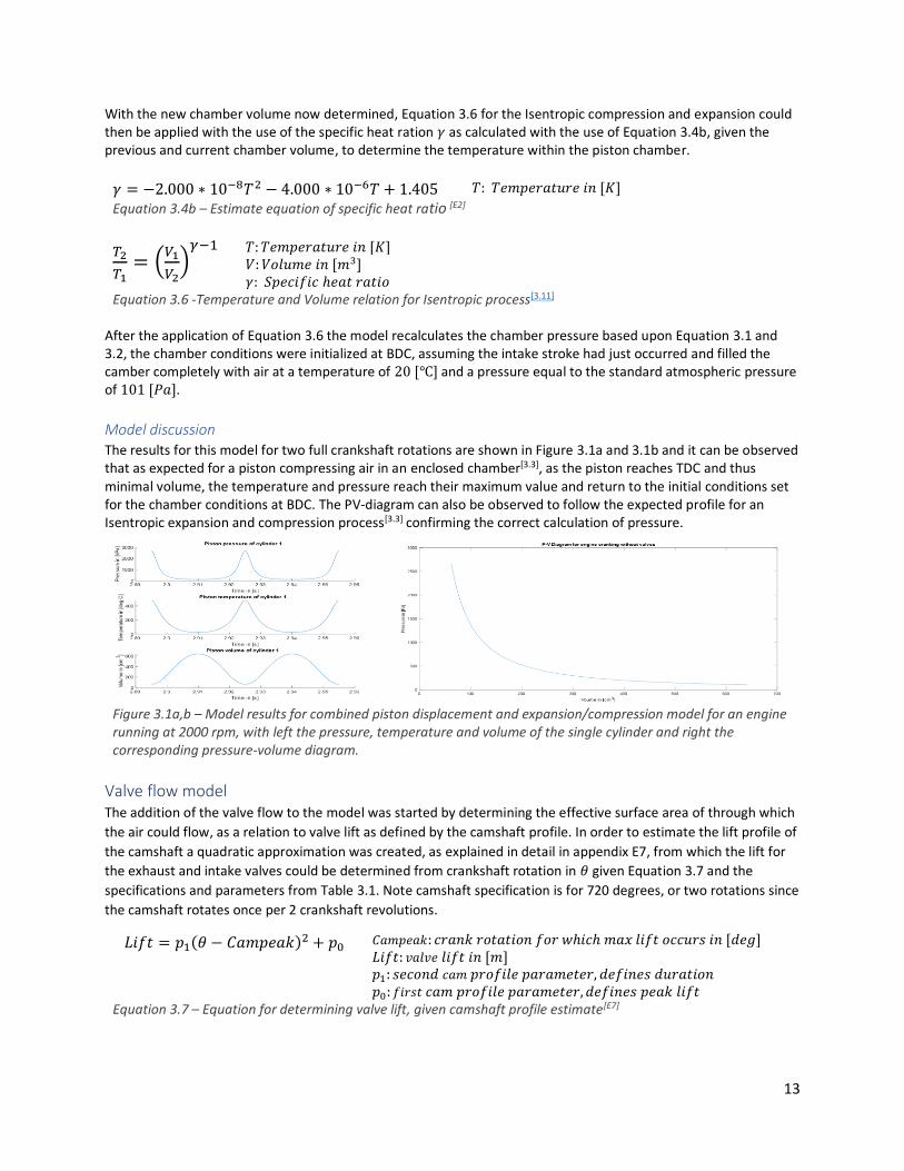
Model discussion The results for this model for two full crankshaft rotations are shown in Figure 3.1a and 3.1b and it can be observed that as expected for a piston compressing air in an enclosed chamber[3.3], as the piston reaches TDC and thus minimal volume, the temperature and pressure reach their maximum value and return to the initial conditions set for the chamber conditions at BDC. The PV-diagram can also be observed to follow the expected profile for an Isentropic expansion and compression process[3.3] confirming the correct calculation of pressure.

Valve flow model The addition of the valve flow to the model was started by determining the effective surface area of through which

the air could flow, as a relation to valve lift as defined by the camshaft profile. In order to estimate the lift profile of

the camshaft a quadratic approximation was created, as explained in detail in appendix E7, from which the lift for

the exhaust and intake valves could be determined from crankshaft rotation in 𝜃 given Equation 3.7 and the

specifications and parameters from Table 3.1. Note camshaft specification is for 720 degrees, or two rotations since

the camshaft rotates once per 2 crankshaft revolutions.

𝐿𝑖𝑓𝑡 = 𝑝1(𝜃 − 𝐶𝑎𝑚𝑝𝑒𝑎𝑘)2 + 𝑝0 𝐶𝑎𝑚𝑝𝑒𝑎𝑘: 𝑐𝑟𝑎𝑛𝑘 𝑟𝑜𝑡𝑎𝑡𝑖𝑜𝑛 𝑓𝑜𝑟 𝑤ℎ𝑖𝑐ℎ 𝑚𝑎𝑥 𝑙𝑖𝑓𝑡 𝑜𝑐𝑐𝑢𝑟𝑠 𝑖𝑛 [𝑑𝑒𝑔] 𝐿𝑖𝑓𝑡: 𝑣𝑎𝑙𝑣𝑒 𝑙𝑖𝑓𝑡 𝑖𝑛 [𝑚] 𝑝1: 𝑠𝑒𝑐𝑜𝑛𝑑 𝑐𝑎𝑚 𝑝𝑟𝑜𝑓𝑖𝑙𝑒 𝑝𝑎𝑟𝑎𝑚𝑒𝑡𝑒𝑟, 𝑑𝑒𝑓𝑖𝑛𝑒𝑠 𝑑𝑢𝑟𝑎𝑡𝑖𝑜𝑛 𝑝0: 𝑓𝑖𝑟𝑠𝑡 𝑐𝑎𝑚 𝑝𝑟𝑜𝑓𝑖𝑙𝑒 𝑝𝑎𝑟𝑎𝑚𝑒𝑡𝑒𝑟, 𝑑𝑒𝑓𝑖𝑛𝑒𝑠 𝑝𝑒𝑎𝑘 𝑙𝑖𝑓𝑡

Equation 3.7 – Equation for determining valve lift, given camshaft profile estimate[E7]

Figure 3.1a,b – Model results for combined piston displacement and expansion/compression model for an engine running at 2000 rpm, with left the pressure, temperature and volume of the single cylinder and right the corresponding pressure-volume diagram.

14

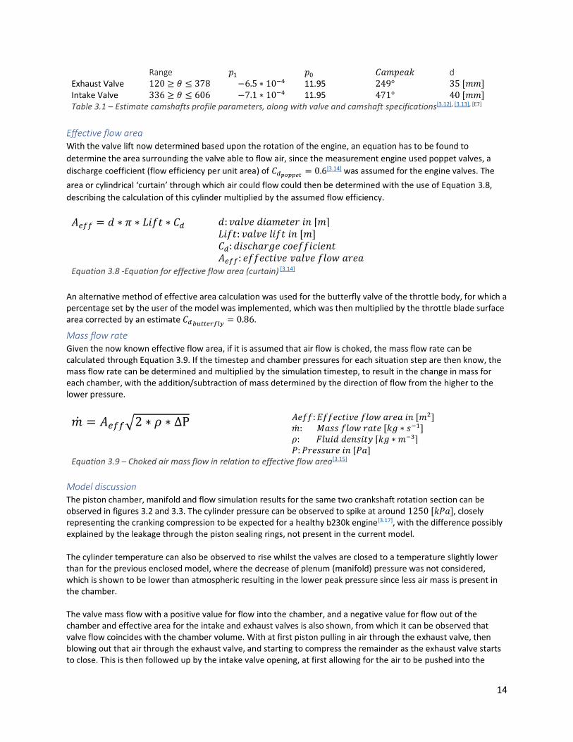
Range 𝑝1 𝑝0 𝐶𝑎𝑚𝑝𝑒𝑎𝑘 d Exhaust Valve 120 ≥ 𝜃 ≤ 378 −6.5 ∗ 10−4 11.95 249° 35 [𝑚𝑚] Intake Valve 336 ≥ 𝜃 ≤ 606 −7.1 ∗ 10−4 11.95 471° 40 [𝑚𝑚] Table 3.1 – Estimate camshafts profile parameters, along with valve and camshaft specifications[3.12], [3.13], [E7]

Effective flow area With the valve lift now determined based upon the rotation of the engine, an equation has to be found to

determine the area surrounding the valve able to flow air, since the measurement engine used poppet valves, a

discharge coefficient (flow efficiency per unit area) of 𝐶𝑑𝑝𝑜𝑝𝑝𝑒𝑡= 0.6[3.14] was assumed for the engine valves. The

area or cylindrical ‘curtain’ through which air could flow could then be determined with the use of Equation 3.8,

describing the calculation of this cylinder multiplied by the assumed flow efficiency.

An alternative method of effective area calculation was used for the butterfly valve of the throttle body, for which a percentage set by the user of the model was implemented, which was then multiplied by the throttle blade surface area corrected by an estimate 𝐶𝑑𝑏𝑢𝑡𝑡𝑒𝑟𝑓𝑙𝑦

= 0.86.

Mass flow rate Given the now known effective flow area, if it is assumed that air flow is choked, the mass flow rate can be calculated through Equation 3.9. If the timestep and chamber pressures for each situation step are then know, the mass flow rate can be determined and multiplied by the simulation timestep, to result in the change in mass for each chamber, with the addition/subtraction of mass determined by the direction of flow from the higher to the lower pressure.

�̇� = 𝐴𝑒𝑓𝑓√2 ∗ 𝜌 ∗ ΔP 𝐴𝑒𝑓𝑓: 𝐸𝑓𝑓𝑒𝑐𝑡𝑖𝑣𝑒 𝑓𝑙𝑜𝑤 𝑎𝑟𝑒𝑎 𝑖𝑛 [𝑚2] �̇�: 𝑀𝑎𝑠𝑠 𝑓𝑙𝑜𝑤 𝑟𝑎𝑡𝑒 [𝑘𝑔 ∗ 𝑠−1] 𝜌: 𝐹𝑙𝑢𝑖𝑑 𝑑𝑒𝑛𝑠𝑖𝑡𝑦 [𝑘𝑔 ∗ 𝑚−3] 𝑃: 𝑃𝑟𝑒𝑠𝑠𝑢𝑟𝑒 𝑖𝑛 [𝑃𝑎]

Equation 3.9 – Choked air mass flow in relation to effective flow area[3.15]

Model discussion The piston chamber, manifold and flow simulation results for the same two crankshaft rotation section can be observed in figures 3.2 and 3.3. The cylinder pressure can be observed to spike at around 1250 [𝑘𝑃𝑎], closely representing the cranking compression to be expected for a healthy b230k engine[3.17], with the difference possibly explained by the leakage through the piston sealing rings, not present in the current model. The cylinder temperature can also be observed to rise whilst the valves are closed to a temperature slightly lower than for the previous enclosed model, where the decrease of plenum (manifold) pressure was not considered, which is shown to be lower than atmospheric resulting in the lower peak pressure since less air mass is present in the chamber. The valve mass flow with a positive value for flow into the chamber, and a negative value for flow out of the chamber and effective area for the intake and exhaust valves is also shown, from which it can be observed that valve flow coincides with the chamber volume. With at first piston pulling in air through the exhaust valve, then blowing out that air through the exhaust valve, and starting to compress the remainder as the exhaust valve starts to close. This is then followed up by the intake valve opening, at first allowing for the air to be pushed into the

𝐴𝑒𝑓𝑓 = 𝑑 ∗ 𝜋 ∗ 𝐿𝑖𝑓𝑡 ∗ 𝐶𝑑 𝑑: 𝑣𝑎𝑙𝑣𝑒 𝑑𝑖𝑎𝑚𝑒𝑡𝑒𝑟 𝑖𝑛 [𝑚] 𝐿𝑖𝑓𝑡: 𝑣𝑎𝑙𝑣𝑒 𝑙𝑖𝑓𝑡 𝑖𝑛 [𝑚] 𝐶𝑑: 𝑑𝑖𝑠𝑐ℎ𝑎𝑟𝑔𝑒 𝑐𝑜𝑒𝑓𝑓𝑖𝑐𝑖𝑒𝑛𝑡 𝐴𝑒𝑓𝑓: 𝑒𝑓𝑓𝑒𝑐𝑡𝑖𝑣𝑒 𝑣𝑎𝑙𝑣𝑒 𝑓𝑙𝑜𝑤 𝑎𝑟𝑒𝑎

Equation 3.8 -Equation for effective flow area (curtain) [3.14]

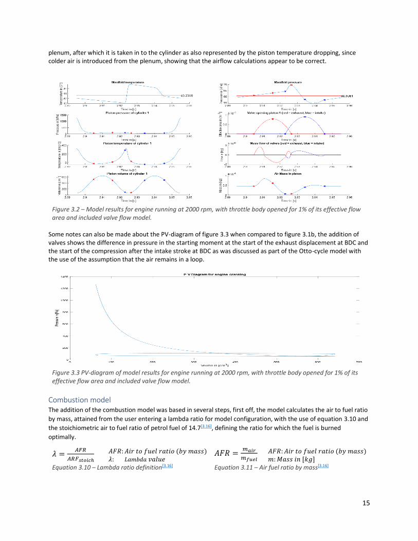
15

plenum, after which it is taken in to the cylinder as also represented by the piston temperature dropping, since colder air is introduced from the plenum, showing that the airflow calculations appear to be correct.

Some notes can also be made about the PV-diagram of figure 3.3 when compared to figure 3.1b, the addition of valves shows the difference in pressure in the starting moment at the start of the exhaust displacement at BDC and the start of the compression after the intake stroke at BDC as was discussed as part of the Otto-cycle model with the use of the assumption that the air remains in a loop.

Figure 3.3 PV-diagram of model results for engine running at 2000 rpm, with throttle body opened for 1% of its effective flow area and included valve flow model.

Combustion model The addition of the combustion model was based in several steps, first off, the model calculates the air to fuel ratio

by mass, attained from the user entering a lambda ratio for model configuration, with the use of equation 3.10 and

the stoichiometric air to fuel ratio of petrol fuel of 14.7[3.16], defining the ratio for which the fuel is burned

optimally.

𝜆 =𝐴𝐹𝑅

𝐴𝑅𝐹𝑠𝑡𝑜𝑖𝑐ℎ 𝐴𝐹𝑅: 𝐴𝑖𝑟 𝑡𝑜 𝑓𝑢𝑒𝑙 𝑟𝑎𝑡𝑖𝑜 (𝑏𝑦 𝑚𝑎𝑠𝑠) 𝐴𝐹𝑅 =

𝑚𝑎𝑖𝑟

𝑚𝑓𝑢𝑒𝑙 𝐴𝐹𝑅: 𝐴𝑖𝑟 𝑡𝑜 𝑓𝑢𝑒𝑙 𝑟𝑎𝑡𝑖𝑜 (𝑏𝑦 𝑚𝑎𝑠𝑠)

𝜆: 𝐿𝑎𝑚𝑏𝑑𝑎 𝑣𝑎𝑙𝑢𝑒 𝑚: 𝑀𝑎𝑠𝑠 𝑖𝑛 [𝑘𝑔] Equation 3.10 – Lambda ratio definition[3.16] Equation 3.11 – Air fuel ratio by mass[3.16]

Figure 3.2 – Model results for engine running at 2000 rpm, with throttle body opened for 1% of its effective flow area and included valve flow model.

16

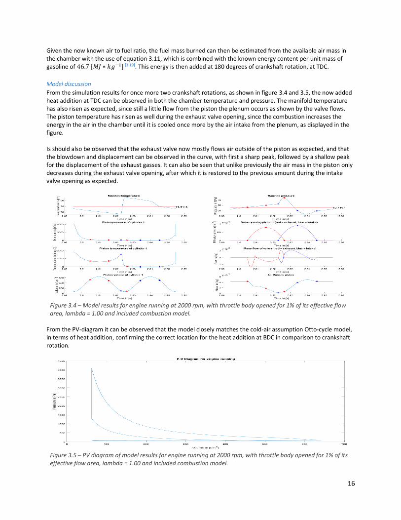
Given the now known air to fuel ratio, the fuel mass burned can then be estimated from the available air mass in the chamber with the use of equation 3.11, which is combined with the known energy content per unit mass of gasoline of 46.7 [𝑀𝐽 ∗ 𝑘𝑔−1] [3.19]. This energy is then added at 180 degrees of crankshaft rotation, at TDC.

Model discussion

From the simulation results for once more two crankshaft rotations, as shown in figure 3.4 and 3.5, the now added heat addition at TDC can be observed in both the chamber temperature and pressure. The manifold temperature has also risen as expected, since still a little flow from the piston the plenum occurs as shown by the valve flows. The piston temperature has risen as well during the exhaust valve opening, since the combustion increases the energy in the air in the chamber until it is cooled once more by the air intake from the plenum, as displayed in the figure. Is should also be observed that the exhaust valve now mostly flows air outside of the piston as expected, and that the blowdown and displacement can be observed in the curve, with first a sharp peak, followed by a shallow peak for the displacement of the exhaust gasses. It can also be seen that unlike previously the air mass in the piston only decreases during the exhaust valve opening, after which it is restored to the previous amount during the intake valve opening as expected.

Figure 3.4 – Model results for engine running at 2000 rpm, with throttle body opened for 1% of its effective flow area, lambda = 1.00 and included combustion model.

From the PV-diagram it can be observed that the model closely matches the cold-air assumption Otto-cycle model, in terms of heat addition, confirming the correct location for the heat addition at BDC in comparison to crankshaft rotation.

Figure 3.5 – PV diagram of model results for engine running at 2000 rpm, with throttle body opened for 1% of its effective flow area, lambda = 1.00 and included combustion model.

17

Multiple cylinders The model was completed with the addition of 3 more cylinders, in offset in initialization and crank angle rotation

as to correspond to the firing order of the b230k engine, with a combustion event occurring every 180 degrees of

crankshaft rotation. All cylinders were configured to take intake air from the plenum, and to exhaust to the

atmosphere.

Model discussion As shown below in figure 3.6, the simulation results for once more 720 degrees of crankshaft rotation, now show 4 spikes in manifold pressure and temperature, corresponding to the 4 cylinders connected to the plenum. It is also shown that the manifold pressure has dropped, since more air is being taken from the manifold, resulting in an observed peak piston pressure of 2500 [𝑘𝑃𝑎], which is close to the expected value for a standard engine under light load of 300 [𝑃𝑠𝑖][3.19] or approximately 2070 [𝑘𝑃𝑎]. This could possibly once more be explained by the lack of a ring leakage model or could possibly be due to the more performance oriented camshaft installed in the engine[3.19]. In additional note on the result, the valve overlap (where both valves are open) can clearly be observed in the manifold pressure and temperature, as shown by the camshaft markers, whilst also being clearly represented in the piston air mass.

Figure 3.6 – Model results for engine running at 2000 rpm, with throttle body opened for 1% of its effective flow area, lambda = 1.00 and including all 4-cylinders.

Parameters from model With the completed model, for which the code and operation overview are available in appendix G3-G5, the parameters to consider for measurement are to be determined. Below a list of the chosen interesting parameters is shown, with a brief explanation of what is assumed to be measurable. Manifold pressure: The manifold pressure is interesting, not only because it allows for an idea of the airflow through the engine, but also shows clear peaks for every 180 degrees of crankshaft rotation and shows the promise of determining valve overlap in the camshaft profile. Manifold temperature: The manifold temperature also shows promising peaks at 180-degree intervals, representing the intake opening, and could possibly for the estimation of the intake warming from the exhaust gasses pushed back into the intake. Piston chamber temperature:

18

The piston temperature is interesting since it shows internal operating heat of the combustion chamber, as well as showing the reversion of the exhaust gas flow for the short section where the exhaust valve is open as the piston is still moving to BDC, possibly allowing for the measurement of the location where the exhaust pressure is equal to the chamber pressure during expansion. Lambda: In order to make a good comparison of model and the to be completed a lambda measurement should be performed, to allow for correct estimation of the fuel quantity burned. Engine speed: In order to get an idea of the airflow through the engine in combination with the pressure signal the engine speed should be measured separately in order to allow for correct model configuration during comparison.

19

The IC Engine: Real-Time Measurement With the from the model determined interesting parameters to be measured, the next step was to attempt real time measurements of these parameters. The selection and placement of measurement sensors will first be discussed, followed by a description of the electronics and code used to process the sensor measurements. After these sections describing the measurement system, the used measurement method will be discussed, concluding with a discussion of mistakes and result validity.

Sensors The first step towards measurement shall be the selection of sensors, starting off with the description of the research done towards the common usage and types of automotive drivetrain sensors, followed by a description of the actually used sensors and concluding with an overview of the placement of these sensors.

Sensor research As a start to the research into common usage of automotive engine sensor, a look was had into the pre-research into engine management sensors, as found in appendix A2. Summarizing, the paper for [A2.1] described spark timing optimization through the use of a crank mounted torque sensor, paper [A2.2] described engine health management for aero engines and was excluded based on its irrelevance. Source [A2.3] discussed the tracking of manifold air pressure for estimation of user experienced torque through two control strategies, paper [A2.4] discussed the control of a valve timing actuator. Resources [A2.5, A2.6, A2.7] were most useful since they discussed the creation of an engine management system and the creation of air-fuel ratio estimators, whilst providing an overview of used engine management signals, with all sources describing the usage of air-fuel ratio (lambda), manifold air pressure (MAP) and engine speeds sensors. To supplement this pre-research a study of prevalence of all available automotive drivetrain sensors was conducted. First a list of the largest automotive sensor producers was created based upon sources [B1.1] and [B1.2], for which for each manufacturer the available sensor types were determined[B1.3-B1.15]. These results can be seen in table 4.1 below.

Table 4.1 – Overview of available automotive drivetrain sensors from major manufacturers (X for available, - for not available) [B1.1-B1.15]

Sensor selection With the now compiled list of commonly used sensors and an idea of the measurements to be considered from the

model, a selection could be made in the sensor types to be used. Below a discussion of use and representative

measurement for each sensor can be found.

Manifold Air Pressure and Temperature

The plenum conditions as shown in the model were decided to be directly measured with the use of a manifold air

pressure and temperature sensor, due to their good availability[B1.3-B1.15], the promise of a good representation of

Producer: Thro

ttle

ope

ning

Cam

/Cra

nk ro

tatio

nAi

rflo

w

Air p

ress

ure

Air t

empe

ratu

reO

xyge

n

Air-

Fuel

Exha

ust

tem

pera

ture

Etha

nol c

onte

ntFu

el te

mpe

ratu

reFu

el p

ress

ure

Oil l

evel

Oil p

ress

ure

Oil t

empe

ratu

reCo

olan

t tem

pera

ture

Knoc

k

Bourns Inc X X - - - - - - - - - - - - - -

Denso Global X X X X - X X X - - X - - - X X

Continental automotive X X X X X - - X X X X X X - X X

Bosch mobility solutions X X - X X X X - - X X X X X X X

Delphi auto parts X X X X - X - X - - - - X X X X

ZF TWR - X - - - - - - - - - - - - - -

Honeywell X X - - X - - X - X - - X X X -

20

the manifold pressure signal due to the fast response of the pressure measuring element with a response time of

𝑡90% = 0.2 [𝑚𝑠] [4.1] and the often found combination of the temperature and pressure sensor in a single sensor

device. The often-integrated temperature sensor commonly has a relatively slow response of 𝑡63% ≤ 45 [𝑠][4.1] and

can therefor only be used to estimate average plenum temperatures.

As for the physical sensor, a Bosch sensor with part number 0 281 002 401 was chosen, since it offered the fast

pressure response time, offered a build in temperature sensor, was easily obtained from common auto parts

dealers and offered a datasheet with calibration curves for measurement interpretation as shown in appendix E4

and E5.

Exhaust Gas Temperature

The piston chamber temperatures were chosen to be indirectly measured through the temperature of the exhaust

gasses, with the use of an exhaust gas temperature sensor, since it allowed for easy integration in the exhaust

system compared to the cylinder head modifications that would be required to install a direct measurement

sensor. These sensors were also shown to be commonly available[B1.3-B1.15], and could be found with fast response

times in the order of 11 [𝑚𝑠] 𝑝𝑒𝑟 300[℃][4.2].

The selected physical sensor was a BM100J-CWE produced by NKT, and was chosen due to its availability from

common auto parts dealers, wide temperature range of 100 − 900 [℃][4.3] and the availability of a datasheet for

measurement interpretation from which the calibration curves can be seen in appendix E3.

Air fuel ratio

The air-fuel mixture was chosen to be measured with the use of a narrowband O2 sensor, which measures excess oxygen in the exhaust path to determine the engine’s operating conditions, which differs for the also commonly available wideband air-fuel ratio sensor in measurement range. However, since the electric fuel injection system installed on the measurement vehicle used the same type of narrowband sensor, it was assumed that the fuel-ratio would remain within sensor measurement range, given the correct operation of the system. The used measurement sensor was a Bosch 0 258 005 097[4.4], a sensor of nearly type to the sensor used by the electric fuel injection system[4.5], with only the addition of an additional measurement ground lead for the sensor element to allow for more sensitive measurement, since the original sensor only offered 1 sensor wire, assuming the grounding occurred through the exhaust system itself. The calibration curves for this sensor can be found in appendix E6.

Engine Speed The engine speed was chosen to be measured through the ignition coil firing moments, which indicate the

approximate occurrence of the combustion event for each cylinder which are as discussed spaced out by 180

degrees of crankshaft rotation. The ignition coil firing was determined through the electronic ignition system that

uses a hall-effect sensor on the crankshaft for identification of the crankshaft rotation, the timing of which is

controlled by many factors[4.6].

No measurement sensors were applied to attain this measurement, instead, a direct connection of the ignition coil

positive was made to the measurement system, for the identification of ignition coil firing moments.

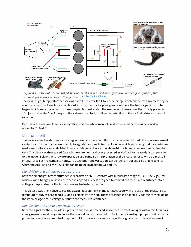
Sensor placement The sensor placement chosen for the final measurement setup can be found in figure 4.1. The manifold air pressure

and temperature sensor were placed right in the middle of the intake plenum, as to detect the airflow from all

cylinders as equally as possible.

21

The exhaust gas temperature sensor was placed just after the 4 to 2 tube merge which on the measurement engine

was made out of not easily modifiable cast iron, right at the beginning section where the two longer 2 to 1 tubes

began, which were made out of more compliable sheet metal. The narrowband sensor was then finally placed in

100 [𝑚𝑚] after the 2 to 1 merge of the exhaust manifold, to allow for detection of the air fuel mixture across all

cylinders.

Pictures of the real-world sensor integration into the intake manifold and exhaust manifold can be found in

Appendix F1.2a-1.2c

Measurement The measurement system was a datalogger based in an Arduino Uno microcontroller with additional measurement

electronics to convert al measurements to signals measurable for the Arduino, which was configured for maximum

read speed of its analog and digital inputs, which were then output via serial to a laptop computer, recording the

data. This data was then stored for each measurement and post processed in MATLAB to create data comparable

to the model. Below the hardware operation and software interpretation of the measurements will be discussed

briefly, for which the complete hardware description and validation can be found in appendix F2 and F3 and for

which the Arduino and MATLAB code can be found in appendix G1 and G2.

Manifold air and exhaust gas temperature

Both the air and gas temperature sensor consisted of NTC-resistors with a calibrated range of 100 − 50𝑘 [Ω], for

which a Wien-bridge circuit as described in appendix F2 was designed to convert the measured resistance into a

voltage interpretable for the Arduino analog to digital converter.

This voltage was then converted to the actual measurement in the MATLAB code with the use of the resistance to

temperature curves of appendix E3 and E4 along with the equations described in appendix F2 for the conversion of

the Wien-bridge circuit voltage output to the measured resistance.

Manifold air pressure and narrowband sensor

Both the signal for the manifold air pressure and the narrowband sensor consisted of voltages within the Arduino’s

analog measurement range and were therefore directly connected to the Arduino’s analog input pins, with only the

protection circuitry as described in appendix F2 in place to prevent damage through short circuits and incorrect

Figure 4.1 - Physical locations of all measurement sensors used on engine, in actual setup, only one of the

exhaust gas sensors was used. [Image credit: [4.7], [4.8], [4.9], [4.10], [4.11]]

22

sensor wiring. These voltages were then converted to the actual air-fuel ratio and pressure with the usage of the

voltage to AFR and voltage to pressure curves as described in appendix E5 and E6.

Engine speed The engine speed was measured through the ignition coil positive wire voltage, which was first attenuated, then limited with limiting diodes and then input into a Schmitt trigger to grab the rising and falling edge for the ignition pulses, as the spark plugs were fired with the circuit as shown in appendix F2. This signal was then directly input into the Arduino’s digital pins, and simply recorded as a quick high low measurement. These high and low values were then converted to a square wave in the MATLAB processing, from which the duration in between rising edge was counted to calculate the engine speed from, assuming each pulse was separated by 180 degrees of crankshaft duration.

Method The measurements were acquired starting off with getting the engine up to operating temperature, with a cooling system in place that kept the engine at a relatively constant temperature. During the measurements the engine was only loaded by its own friction and the rotating mass of the flywheel, clutch and transmission in neutral gear. Measurements were acquired for an engine rotation speed of 1000 – 5000 [rev/s] which was increased in steps of 500 [rev/s] for each measurement. Each measurement was started with the engine left to idle for approximate 20 seconds, after which the throttle was opened and maintained at a position for which the correct engine rotation speed was reached. The given measurement speed was then maintained for 10 seconds, to allow for all measurements to stabilize, after which the engine was once more left to idle for approximately 20 second concluding the measurement run. An overview of the complete measurements for each engine speed after processing in MATLAB can be found in appendix D1.1-D9.1. From these complete measurement runs, selections of 5 second sections with relatively constant engine speed close to the desired measurement speed was made, of which the results are shown in appendix D1.2-D9.2. Additionally, to these selected sections and fast Fourier transform was also applied, resulting in the frequency spectra as found in appendix D1.4-D9.4. Since for comparison to the model a closer view of two crankshaft rotations was also required, a section from the already selected 5 second period was taken wherein the measured air to fuel ratio was relatively constant. From these sections, an equivalent time duration to 2.5 crankshaft rotations at the specified measurement engine speed was selected, of which the results are shown in appendix D1.6 – D9.6.

Discussion

Correction factor After measurement a required correction factor was discovered by comparing the ‘measured’ frequency with original timestamp with expected values determined from calculation as seen in table 4.2 below. After plotting results against each other a ratio was suspected, and after averaging a ratio of 3.367 was determined, the offset value for 5000 [rev/min] can probably explained by a lower average speed successfully maintained, as is shown in appendix D9.1. This correction factor was caused by an error in the Arduino code, in placing the timer for each measurement, such that the serial write time would not be considered, resulting in a lower actual sample rate than told by the data, since the serial write time was significantly longer than the measurement time.

Engine speed in [rev/min] 1000 1500 2000 2500 3000 3500 4000 4500 5000

Calculated in [Hz] 33.33 50.00 66.67 83.33 100.00 116.67 133.33 150.00 166.67

Measured in [Hz] 112.88 172.29 226.38 283.27 339.75 399.16 454.42 501.42 519.14

Ratio Measured/Expected 3.386 3.446 3.396 3.399 3.397 3.421 3.408 3.343 3.115

4.2 – Table with measured ignition pulses versus calculated expected ignition pulses from rpm

23

The validity of the results in Appendix D could be argued, but since ratio appears to be reasonably stable with engine speed, and since for the comparison of the frequency spectrum peaks of the model and measurements close results can still be observed between model and processed measurements, enough can still be said about the signal, although a more accurate timestamp would be desirable in the future.

Achieved Sample rate

As shown in table 4.3 below, the achieved sample rate ended up at 492 [𝐻𝑧] average, which is less than would be desirable given the 𝑡90% = 0.2 [𝑚𝑠] [4.1] response time for the pressure sensor, which would require a minimum sampling frequency of 5 [𝑘𝐻𝑧]. From which it can be concluded that the full potential of the MAP sensor has not yet been achieved, which also unfortunately affected the usability of the 2.5 crankshaft rotation duration measurements in Appendix D. Since the integrated MAT sensor had a response time of 𝑡63% ≤ 45 [𝑠][4.1] from which it can be concluded its measurement resolution was not affected by the slower sample rate.

Since no response time was given in the EGT sensor datasheet for the used sensor, it cannot be said if it was sampled quick enough, but assuming the 11 [𝑚𝑠] 𝑝𝑒𝑟 300[℃][4.2] provided by competitive sensors a minimum sampling speed of 90 [𝐻𝑧] would be required, which would be satisfied with the current measurement results. Since the lambda sensor datasheet specified no response time, the response time from another source is assumed, which was equal to 2 [𝑠] [4.12], for which the sample rate is more than adequate.

Engine speed [rev/min] 1000 1500 2000 2500 3000 3500 4000 4500 5000 Average:

Sample rate in [Hz] 493 490 490 491 487 494 495 496 491 492

4.3 – Table with engine speed for measurement versus sample rate for measurement.

24

Operating Conditions: Theory vs Practice In order to verify the correspondence of the model and the measurements, to allow for later verification of

suggested methods of parameter extraction, a discussion will follow comparing all measured parameters to their

corresponding model equivalents.

For this comparison the waveforms appendix D2.2 and D2.3 were taken since they offer a close up view of

measurements in comparison to the simulation, for the comparison of the frequency spectra D.6 and D.7 were

taken since they offered the highest spectra resolution as they were based on the longer section simulation and

measurement of D2.4 and D2.5.

An engine speed of 1500 [𝑟𝑒𝑣

𝑚𝑖𝑛] was chosen for the base comparison of results since it sat high enough above the

idle speed to prevent engine management system interference through accidental entering of the idle condition at

800 [𝑟𝑒𝑣

𝑚𝑖𝑛] and allowed for as many samples as possible for the measured waveforms since the sample frequency

was limited. For the all measurements compared to simulation the same engine speed, average lambda and

averaged manifold pressure (as fine-tuned by the alteration of the throttle body configuration in the model until a

reasonable match was achieved) were configured in the model, to allow for fair comparison.

Manifold Air Pressure First of we will discuss the manifold air pressure measurements, since these showed the most promise in the model

discussion as well as offered the highest response speed, with a much higher potential than the sample speed

achieved.

Waveform A comparison of the measured and simulated manifold air pressure is shown below in figure 5.1a and b as taken

from appendix D2.6 and D2.7.

Figure 5.1a – Measured manifold air pressure as taken from appendix D2.6

Figure 5.1b – Simulated manifold air pressure as taken from appendix D2.7

As can be observed in the figures, the profile of the measurement coincides rather well, but appears to suffer from the low sample rate. This similarity of waveform shape is also observed in the comparison of the measured manifold pressures when compared to the model for all other measurement engine speeds from appendix Dx.6 and Dx.7 from which it can be concluded that the model is fairly accurate, as even the range across which the pressure is observed to vary is matched. It also becomes apparent when comparing the waveform for all engine speeds, that as the number of available samples to represent the waveform shape decreases with engine speed, less information about the pressure waveform becomes available, and that for future measurements a higher sample rate would be desirable.

Frequency spectrum A comparison of the measured signal frequency spectrum and the simulation frequency spectrum can be observed

below in figure 5.2a and b as taken from appendix D2.4 and D2.5.

25

Figure 5.2a – Measured manifold pressure frequency spectrum as taken from appendix D2.4

Figure 5.2b – Simulated manifold pressure frequency spectrum as taken from appendix D2.5

As can be observed in the figures, a first, second and third harmonic as determined from the simulation, can also clearly be observed in the measured signal, with even a fourth harmonic observable to coincide. However, an additional low frequency peak, which was neglected since it could be explained to be fluctuation in the throttle body position as caused by difficulty in holding the steady rpm with the throttle pedal for a 10 second section, since the variation has a very low frequency of 0.8 [𝐻𝑧].

Figure 5.3 – Graph of comparison of first harmonic observed in frequency spectra for measurements and simulations as taken from appendix H2.1

As can be observed in figure 5.3 above the first harmonic observed in the manifold pressure from the measurements and the model coincide really well, with worsening deviation occurring as engine speed increases, possibly explained by the low sample count. This can also clearly be observed in the manifold pressure waveform in appendix D6.6, D7.6, D8.6 and D9.6 where the waveform becomes less representative of the expected model with each increase in engine speed.

Figure 5.4 – Graph of comparison of second harmonic observed in frequency spectra for measurements and simulations as taken from appendix H2.2

0.0

50.0

100.0

150.0

200.0

0 1000 2000 3000 4000 5000 6000

Freq

uen

cy in

[H

z]

Engine Speed in [rev/s]

Comparison of measured vs modelled 1st harmonic

Measured main harmonic

Modelled main harmonic

0.0

100.0

200.0

300.0

0 500 1000 1500 2000 2500 3000 3500 4000Freq

uen

cy in

[H

z]

Engine Speed in [rev/s]

Comparison of measured vs modelled 2nd harmonic

Measured second harmonic

Modelled second harmonic

26

The good coincidence for the second harmonic of the lower engine speeds measurement and simulation is shown in figure 5.4, where only the engine speeds for which the measured harmonic still fell within the available frequency range to be correctly measured of half of the sample rate, due to the Nyquist-criterium are shown. The worsening deviation is not shown, since the affected engine speeds measurements have no second harmonic within the measurable frequency range.

Figure 5.5 – Graph of comparison of third harmonic observed in frequency spectra for measurements and simulations as taken from appendix H2.3

The good coincidence for the third harmonic of the lower engine speeds measurement and simulation is shown in figure 5.5, with only the third harmonics of the first three engine speeds measured falling within the measurable frequency range. In conclusion it can be said that the model and measurement harmonics are expected to coincide well even for the higher frequencies as the sample rate is increased, and the resolution of the manifold pressure signal is restored for the higher engine speeds, confirming once more that the model appears accurate for the simulation of the manifold pressure signal.

Manifold Air Temperature A comparison of the measured and simulated manifold air temperatures is shown below in figure 5.6a and b as taken from appendix D2.6 and D2.7.

Figure 5.6a – Measured manifold air temperature as

taken from appendix D2.6 Figure 5.6b – Simulated manifold air temperature as taken from appendix D2.7

As can be observed in the figures, as expected the measurement sensors response is relatively slow resulting in a relatively constant temperature measurement, without the expected peaks as observed in the model. It is also to be noted that the simulated intake manifold temperature is much higher, which can be observed in appendix D2.7 as caused by the pressure differential between the intake manifold and the atmosphere air, allowing air to flow from the exhaust to the intake as shown by the air flow from the exhaust into the piston and by the airflow from the piston to the plenum. This is different in reality since the exhaust system is often not at atmospheric pressure, since the exhaust manifold is configured is such a manner (the 4-2-1 configuration as shown in the sensor description) that the exhaust pulses create a low pressure at the exhaust port at just the right time during the valve overlap, to pull more of the exhaust gasses out of the chamber[5.1].

0.0

50.0

100.0

150.0

200.0

250.0

0 500 1000 1500 2000 2500

Freq

uen

cy in

[H

z]

Engine Speed in [rev/s]

Comparison of measured vs modelled 3rd harmonic

Measured third harmonic

Modelled third harmonic

27

Figure 5.7 – Graph of comparison of average measured and simulated intake temperatures along with air fuel ratio’s as taken from appendix H3.2

As shown in the figure 5.7, even though the incorrect modelling of the exhaust flow without the use of the scavenging effect, a rise in intake air temperature is observed both in the measurement and simulation as the lambda value decreases, and thus a richer mixture (more fuel) is introduced into the combustion chamber. This is as would be expected since the net amount of heat per combustion event would be increased since more fuel is allowed to be burned to produce energy, proving that the model behavior still coincides with expectation, although exact relations are not maintained when an exhaust system is attached to the engine that instead of venting the exhaust directly to the atmosphere, requiring care when comparing measurement and the model concerning intake temperatures.

Exhaust Gas Temperature A comparison of the measured exhaust gas temperature and simulated combustion chamber temperature temperatures is shown below in figure 5.8a and b as taken from appendix D2.6 and D2.7.

Figure 5.8a – Measured exhaust gas temperature as taken from appendix D2.6

Figure 5.8b – Simulated piston chamber temperature as

taken from appendix D2.6 As can be observed in the figure, the exhaust temperature is observed to be higher as the average combustion chamber temperature, as is expected, however when observing appendix D2.6, is can be seen that the section for which the exhaust valve is opened is approximated by the area where the piston chamber temperature is in between 500 − 1000 [℃], which would result in the observed approximate average of 700 [℃]. It should also once more be noted that the not modelled exhaust reversion would result in more hot exhaust flow right at the section of valve overlap where it can be observed that the chamber temperatures are around 1000 − 1250[℃], adding to the expected exhaust gas temperature heat, which is now added to the plenum in the model as shown previously.

0.85

0.9

0.95

1

1.05

1.1

0

50

100

150

200

Tem

per

atu

re in

[°C

]

Engine Speed in [rev/s]

Lambda versus Intake Temperature

Measured MAT

Model MAT

Air Fuel ratio (Lambda)

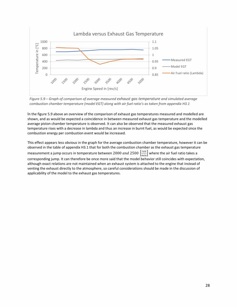
28

Figure 5.9 – Graph of comparison of average measured exhaust gas temperature and simulated average

combustion chamber temperature (model EGT) along with air fuel ratio’s as taken from appendix H3.1 In the figure 5.9 above an overview of the comparison of exhaust gas temperatures measured and modelled are

shown, and as would be expected a coincidence in between measured exhaust gas temperature and the modelled average piston chamber temperature is observed. It can also be observed that the measured exhaust gas temperature rises with a decrease in lambda and thus an increase in burnt fuel, as would be expected since the combustion energy per combustion event would be increased. This effect appears less obvious in the graph for the average combustion chamber temperature, however it can be observed in the table of appendix H3.1 that for both the combustion chamber as the exhaust gas temperature

measurement a jump occurs in temperature between 2000 𝑎𝑛𝑑 2500 [𝑟𝑒𝑣

𝑚𝑖𝑛] where the air fuel ratio takes a

corresponding jump. It can therefore be once more said that the model behavior still coincides with expectation, although exact relations are not maintained when an exhaust system is attached to the engine that instead of venting the exhaust directly to the atmosphere, so careful considerations should be made in the discussion of applicability of the model to the exhaust gas temperatures.

0.85

0.9

0.95

1

1.05

1.1

0

200

400

600

800

1000

Tem

per

atu

re in

[°C

]

Engine Speed in [rev/s]

Lambda versus Exhaust Gas Temperature

Measured EGT

Model EGT

Air Fuel ratio (Lambda)

29

Operating Conditions: Extraction With the correspondence of the model with the measurements for the manifold air pressure now confirmed, and the confirmation of similar to expected behavior for the exhaust and intake temperatures, a methodology and analysis for the extraction of engine operating conditions can be suggested.

Engine speed Starting off with one of the most important measurements for the determination of engine operation, the engine speed, a method is proposed for the extraction of this parameter through the use of the frequency transform of the manifold air pressure signal as shown below in figure 6.1.

𝐸𝑛𝑔𝑖𝑛𝑒 𝑆𝑝𝑒𝑒𝑑 =

𝑓𝑚𝑒𝑎𝑠𝑢𝑟𝑒𝑑

𝑥∗ 60

Figure 6.1 – Measured manifold pressure frequency spectrum as taken

from appendix D2.4 for an engine speed off 1500 [rev

min]

Equation 6.1 – Proposed engine speed calculation

As shown in the figure the main frequency measured is around 52 [𝐻𝑧]. Given that the pressure peaks observed represent the intake being open and air flowing from the piston into the plenum, equation 6.1 could be applied to extract the expected engine speed from the frequency measurement, with the factor x being dependent on engine configuration which represent the occurrence of intake valve openings per crankshaft rotation. Below in table 6.1 the application of equation 6.1 to all performed measurements with 𝑥 = 2 as is appropriate for the measurement engine can be found.

Average measured engine speed in [rev/min]

983 1561 2026 2551 3066 3614 4033 4514 4576

Measured main frequency of manifold air pressure in [Hz]

33.2 52.6 68.7 85.0 102.3 122.1 130.8 153.5 169.8

Calculated engine speed in [rev/min]

996 1578 2061 2550 3069 3663 3924 4605 5094

Table 6.1 – Measured engine speed as taken from appendix Dx.2 compared to engine speed as calculated with equation 6.1 from measured main manifold air pressure frequency as taken from appendix H2.1

It can be observed in table 6.1 that the calculated and measured engine speed coincide rather well, with more deviation shown towards the highest engine speeds, which is probably due to the measurement inaccuracy due to the low sample rate as discussed in the previous chapter. From these results it can be said that equation 6.1 appears to hold, thereby proving that the engine speed could be extracted from the manifold air pressure sensor signal.

30

Engine rotation The next important engine parameter to consider is the engine rotation, as often defined in crankshaft degrees, which allows the engine management system to determine engine rotation, which is commonly used for the determination of ignition timing and fuel injection timing[6.1], [6.2]. It is proposed that by the determination of key markers in the manifold air pressure signal an estimation of engine rotation could be achieved.

Figure 6.2a – Simulated manifold air pressure as taken from appendix D2.7

Figure 6.2b – Measured manifold air pressure as taken from appendix D2.6

From figure 6.2a and b above, and the discussed coincidence of the model with the manifold air pressure measurement, a look could be had at the camshaft markers as shown in figure 6.2a when compared to the measurements. It can be observed that the peaks and lows correspond to the opening of the intake and the closing of the exhaust valve as shown in appendix D2.7, which would allow for an accurate reference, since the timing in between intake closing and opening is well defined in degrees. With the use of this reference, and the knowledge of the valve opening occurrence spacing for each cylinder an estimate of the rotation rate in degrees per second for the engine could be determined with the use of equation 6.2 below.

𝑟𝑜𝑡𝑎𝑡𝑖𝑜𝑛 𝑟𝑎𝑡𝑒 =𝑜𝑣𝑒𝑟𝑙𝑎𝑝

(𝑡𝑝𝑒𝑎𝑘𝑚𝑖𝑛−𝑡𝑝𝑒𝑎𝑘𝑚𝑎𝑥)

𝑟𝑜𝑡𝑎𝑡𝑖𝑜𝑛 𝑟𝑎𝑡𝑒: 𝑒𝑛𝑔𝑖𝑛𝑒 𝑟𝑜𝑡𝑎𝑡𝑖𝑜𝑛 𝑟𝑎𝑡𝑒 𝑖𝑛 [°

𝑠]

𝑜𝑣𝑒𝑟𝑙𝑎𝑝: 𝑑𝑢𝑟𝑎𝑡𝑖𝑜𝑛 𝑖𝑛 [°]𝑓𝑜𝑟 𝑤ℎ𝑖𝑐ℎ 𝑏𝑜𝑡ℎ 𝑣𝑎𝑙𝑣𝑒𝑠 𝑎𝑟𝑒 𝑜𝑝𝑒𝑛 𝑡𝑝𝑒𝑎𝑘: 𝑡𝑖𝑚𝑒 𝑖𝑛 [𝑠] 𝑓𝑜𝑟 𝑤ℎ𝑖𝑐ℎ 𝑝𝑒𝑎𝑘 𝑖𝑛 𝑚𝑎𝑛𝑖𝑓𝑜𝑙𝑑 𝑝𝑟𝑒𝑠𝑠𝑢𝑟𝑒 𝑜𝑐𝑐𝑢𝑟𝑠

Equation 6.2 – Proposed equation for calculation of crankshaft rotation rate

With the determined rotation rate, and knowledge of the camshaft profile compared to engine rotation, either the peak at the maximum or at the minimum of the manifold air pressure measurement could be used as a steady reference from which to continuously determine actual crankshaft rotation. The only problem to be considered is the determination of the cylinder for which the maxima occurs, since a starting reference is required to determine which cylinder is first observed. This could possibly be solved by placing the pressure sensor closer to one of the cylinders, which would be expected to result in a stronger measurement of the pressure differential as caused by this cylinder.

Camshaft profile. Another possibly determinable engine parameter would be the profile of the camshaft given the above provided measurement of engine rotation, for which the simulated profile and valve flows can be observed in figure 6.3 below.

Figure 6.3 – Simulated camshaft profile and valve mass air flow (positive = into piston, negative = out of piston) as taken from appendix D2.7

As shown previously the peaks of the manifold air pressure measurements correspond well to the intake valve opening and exhaust valve closing as shown in figure 6.2a through the camshaft markers as corresponding to the

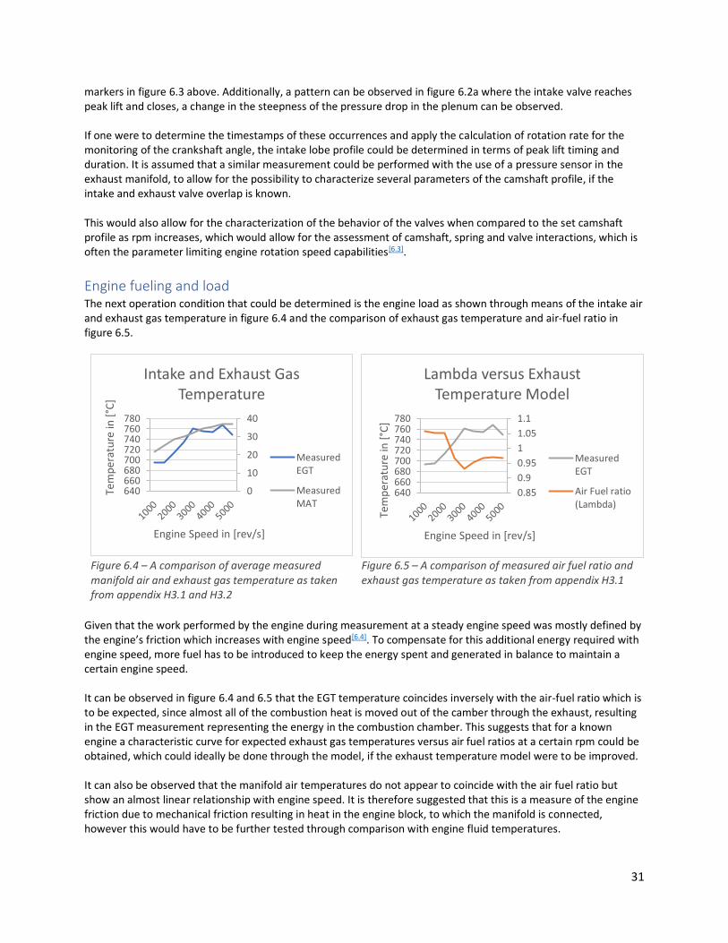
31

markers in figure 6.3 above. Additionally, a pattern can be observed in figure 6.2a where the intake valve reaches peak lift and closes, a change in the steepness of the pressure drop in the plenum can be observed. If one were to determine the timestamps of these occurrences and apply the calculation of rotation rate for the monitoring of the crankshaft angle, the intake lobe profile could be determined in terms of peak lift timing and duration. It is assumed that a similar measurement could be performed with the use of a pressure sensor in the exhaust manifold, to allow for the possibility to characterize several parameters of the camshaft profile, if the intake and exhaust valve overlap is known. This would also allow for the characterization of the behavior of the valves when compared to the set camshaft profile as rpm increases, which would allow for the assessment of camshaft, spring and valve interactions, which is often the parameter limiting engine rotation speed capabilities[6.3].

Engine fueling and load The next operation condition that could be determined is the engine load as shown through means of the intake air and exhaust gas temperature in figure 6.4 and the comparison of exhaust gas temperature and air-fuel ratio in figure 6.5.

Figure 6.4 – A comparison of average measured manifold air and exhaust gas temperature as taken from appendix H3.1 and H3.2

Figure 6.5 – A comparison of measured air fuel ratio and exhaust gas temperature as taken from appendix H3.1

Given that the work performed by the engine during measurement at a steady engine speed was mostly defined by the engine’s friction which increases with engine speed[6.4]. To compensate for this additional energy required with engine speed, more fuel has to be introduced to keep the energy spent and generated in balance to maintain a certain engine speed. It can be observed in figure 6.4 and 6.5 that the EGT temperature coincides inversely with the air-fuel ratio which is to be expected, since almost all of the combustion heat is moved out of the camber through the exhaust, resulting in the EGT measurement representing the energy in the combustion chamber. This suggests that for a known engine a characteristic curve for expected exhaust gas temperatures versus air fuel ratios at a certain rpm could be obtained, which could ideally be done through the model, if the exhaust temperature model were to be improved. It can also be observed that the manifold air temperatures do not appear to coincide with the air fuel ratio but show an almost linear relationship with engine speed. It is therefore suggested that this is a measure of the engine friction due to mechanical friction resulting in heat in the engine block, to which the manifold is connected, however this would have to be further tested through comparison with engine fluid temperatures.

0

10

20

30

40

640660680700720740760780

Tem

per

atu

re in

[°C

]

Engine Speed in [rev/s]

Intake and Exhaust Gas Temperature

MeasuredEGT

MeasuredMAT

0.85

0.9

0.95

1

1.05

1.1

640660680700720740760780

Tem

per

atu

re in

[°C

]

Engine Speed in [rev/s]

Lambda versus Exhaust Temperature Model

MeasuredEGT

Air Fuel ratio(Lambda)

32

Concluding To conclude the analysis into possible improvements in the use of automotive sensors in an electronic fuel injection

and ignition system, we will first list a summary of the achievements during this analysis, after which an attempt

will be made to answer the research thesis, which will be followed by a suggestion of further steps into the

developments of the suggested improvements.

Achievements During the analysis the first major achievement was the creation of a more accurate model for the 4-stroke Otto-

cycle engine with the ability to model multiple cylinders, camshaft profiles, plenum pressure and temperature

behavior and configurability of engine speed and air-fuel ratio, that could be verified to match with engine

operation theory.

The second major achievement was the creation of a real time measurement system, capable of measuring

manifold air pressure, manifold air temperature, exhaust gas temperature, air-fuel ratio’s and engine speed at a

sampling rate of 490 [𝐻𝑧].

The third major achievement was the combination of the model and measurement results with the theory of

engine operation to result in suggested methodologies for the extraction of engine speed and crankshaft rotation

from the manifold air pressure sensor, the extraction of engine fueling through the use of an exhaust gas

temperature sensor, and the suggested extraction of engine friction through the intake air temperature sensor.

Thesis discussion With the above stated achievements in mind, an attempt will be made to answer the thesis as stated in the introduction:

“Given the modern processing, modelling and measurement capabilities, a reduction of sensors used and

additional control for internal combustion engine management can be achieved through the extraction of

multiple key engine operating parameters from a single sensor”

Provided that during the third chapter clear proof was provided of the feasibility of the usage of the manifold air

pressure for the measurement of not only the average pressure, but also for the measurement of the engine speed

and crank rotation with clever sensor placement, allowing for the extraction of multiple key engine operation

parameters from a single sensor. The possibility of which was deducted through the comparison of a model created

in a modern modelling environment with the now commonly available fast real time measurement and post

processing of operation parameters. It could confidently be argued that the thesis statement could be argued valid.

Suggested additional development As suggested earlier, an exhaust manifold model could possibly be added to the engine model to more accurately

represent the airflow through the exhaust valves with the addition of exhaust scavenging, which should also

improve the accuracy of the modelled intake air temperature and the airflow during the exhaust and intake

overlap, allowing for better comparison of the measurements to the model.

As to the sensors are concerned, improvements could be made with faster response time temperature sensors as was shown in the section on interesting measurable quantities as shown in the model chapter, where the chamber temperature and intake air temperature both showed possibly useful waveform characteristics. Additionally, a measurement of the engine cylinder wall temperatures could be included to allow for comparison of the intake air temperature to the friction of the engine as was proposed previously. For the measurements it would be highly be recommended to increase the achieved sample rate to faster than the

response of the pressure sensor, to allow for more detailed comparison to the model results.

References Below all used reference are to be found, the references are numbered starting at 1 for each chapter.

[1.1] Tuomi, Ilkka.”The lives and death of Moore’s Law” 4 November 2002. Webpage describing a benchmark for the advancements in processing power. Visited: 18-01-2019. <https://firstmonday.org/ojs/index.php/fm/article/view/1000/921> [1.2] Mathworks Inc. “A Brief History of MATLAB” 2018. Webpage describing the history of the modelling capabilities of the MATLAB software package. Visited: 18-01-2019. <https://nl.mathworks.com/company/newsletters/articles/a-brief-history-of-matlab.html> [1.3] Bosch. “Bosch MEMS Sensor” 2018. Webpage describing the history of the Bosch MEMS sensor. Visited: 18-01-2019. <https://www.bosch-mobility-solutions.com/en/products-and-services/industry-elements-and-components/mems-sensors/> [1.4] NGK. “Exhaust Gas Temperature Sensors” 2016. Webpage describing NGK’s 4th generation of exhaust gas temperature sensors with a description of sensor advancements. Visited: 18-01-2018. <https://www.ngk.com.au/products/exhaust-gas-temerature-sensor/> [1.5] European Union. “Road transport: Reducing CO2 emissions from vehicles” Webpage describing current European Union policy on emissions for road vehicles. Visited: 18-01-2019. <https://ec.europa.eu/clima/policies/transport/vehicles_en> [1.6] The Economist. “The Death of the Internal Combustion Engine” 12 August 2017. Article discussing the gradual change from vehicles to electrical drive. Visited: 18-01-2019. <https://www.economist.com/leaders/2017/08/12/the-death-of-the-internal-combustion-engine> [1.7] Wikipedia. “Car Tuning” 18 November 2018. Webpage describing the activity of car tuning. Visited: 18-01-2019. <https://en.wikipedia.org/wiki/Car_tuning> [1.8] Wikipedia. “Motorcycling” 10 November 2018. Webpage describing the activity of Motorcycling. Visited: 18-01-2019. <https://en.wikipedia.org/wiki/Motorcycling> [1.9] Wikipedia. “Fuel Injection” 20 December 2018. Webpage describing the concept of fuel injection including historical development, application and operating principles. Visited: 18-01-2019. <https://en.wikipedia.org/wiki/Fuel_injection> [1.10] Wikipedia. “Ignition System” 22 January 2019. Webpage describing the concept of ignition systems including historical development, application and operating principles. Visited: 18-01-2019. <https://en.wikipedia.org/wiki/Ignition_system> [1.11] National Automotive Parts Association. “Carburetor vs Fuel Injection – Short History and Pros & Cons” 30 June 2016. Webpage describing an historical comparison of carburetors compared to fuel injection and their pros and cons. Visited: 18-01-2019. <http://knowhow.napaonline.com/carburetor-vs-fuel-injection-short-history-pros-cons/> [1.12] Springer. “Ignition systems over the years” 2015. Article describing the advancements in ignition systems across the years” Visited: 18-01-2019. <https://link.springer.com/content/pdf/10.1007%2F978-3-658-03964-6_10.pdf>

[2.1] Cambridge University Engineering Department. “The Early History of Combustion Engines” 2002. Webpage on the history of the combustion engine. Visited: 16-01-2019. <http://www3.eng.cam.ac.uk/DesignOffice/projects/cecil/history.html> [2.2] Maison Nicéphore Niépce. “Le pyréolophore” Webpage on the history of the pyréolophore by the Niépce brothers. Visited 16-01-2019. <http://www.photo-museum.org/fr/pyreolophore-invention-moteur-explosion/> [2.3] Nicolaus-Augustus-Otto.de (Archived version). “125 Jahre Viertaktmotor” 2009. Webpage archive on Nicolaus Otto and his engine. Visited: 16-01-2019. <https://web.archive.org/web/20110507083259/http:/www.nicolaus-august-otto.de/node/15> [2.4] Daimler Group. “Company History; Benz Patent Motor Car: The first automobile (1885-1886). 2019. Webpage on history of first automobile. Visited: 16-01-2019. <https://www.daimler.com/company/tradition/company-history/1885-1886.html> [2.5] Jääskeläinen, Hannu. “Early History of the Diesel Engine” 19-11-2013. Webpage on early Diesel engine history. Visited: 16-01-2019. <https://www.dieselnet.com/tech/diesel_history.php> [2.6] Pope, A., "The Hesselman Low-Compression Diesel-Fuel-Burning Engine," SAE Technical Paper 340111, 1934, <https://doi.org/10.4271/340111> [2.7] Craig’s Rotary Page. “NSU Wankel rotary engines and cars” 17-01-2001. Webpage on history of Wanke engine. Visited: 16-01-2019. <http://cp_www.tripod.com/rotary/pg05.htm> [2.8] Daimler-Benz AG. “Vorrichtung an einem in einem kurbelgehaeuse eingesetzten kurbeltrieb” 22-07-2019. Patent: DE3624753A1. <https://patents.google.com/patent/DE3624753A1/de> [2.9] Marotta Marco. “Mazda HCCI Engine” 2017. Webpage article on new Mazda engine for Drivetribe. Visited: 16-01-2019. <https://drivetribe.com/p/mazda-hcci-engine-eg4HHogdQg20qxRJ4e0QVA?iid=FR31MOHGQteCFZAlYN6Jmg> [2.10] Proctor, Charles Lafayette. “Internal Combustion Engine” 15 January 2018. Encyclopedia Britannica webpage about internal combustion engine. Visited: 16-01-2019. <https://www.britannica.com/technology/internal-combustion-engine> [2.11] Haynes. “Beginner's Guide: What Is a Four Stroke Engine (and How Does It Work)?” 21 February 2018. Webpage about the 4-stroke engine. Visited: 16-01-2019. <https://haynes.com/en-us/tips-tutorials/beginners-guide> [2.12] Goel, Tarun. “How to Calculate the Stoichoimetric Air-Fuel Ratio” Webpage about Air-Fuel ratio calculation for various fuels. Visited: 16-01-2019. <https://www.brighthubengineering.com/machine-design/15235-the-stoichiometric-air-fuel-ratio/> [2.13] CarBikeTech. “What Is Volumetric Efficiency? Volumetric Efficiency Vs Mechanical Efficiency” 31 May 2018. Webpage on the topic of volumetric efficiency and its meaning to internal combustion engine. Visited 17-01-2019. <https://carbiketech.com/volumetric-efficiency-mechanical-efficiency/> [2.14] Britannica’s Editorial Staff. “Compression Ratio” 01 December 2014. Webpage on compression ratio by encyclopedia Britannica. Visited 17-01-2019. <https://www.britannica.com/technology/compression-ratio> [2.15] Khemani, Haresh. “Spark Ignition (SI) Engine and Compression Ignition (CI) Engine: A Comparison” Webpage on comparison of Spark Ignition and Compression Ignition Engines. Visited: 17-01-2019.

[2.16] Brooking, Gerard. “Ideal Intake and Exhaust Strokes” 2015. Presentation concerning ideal intake and exhaust strokes. Visited: 17-01-2019. <https://slideplayer.com/slide/1709937/> [2.17] Khemani, Haresh. “Two-Stroke Engines: Advantages and Disadvantages” Webpage containing discussion of advantages and disadvantages of the two-stroke engine. Visited: 17-01-2019. <https://www.brighthubengineering.com/machine-design/1513-advantages-and-disadvantages-of-two-stroke-engine/> [2.18] Encyclopedia Britannica. “Two-Stroke Engine” Webpage containing an illustration of the two-stroke engine operating principle. Visited 17-01-2019. <https://www.britannica.com/technology/two-stroke-cycle> [2.19] Cycleworld – two stroke motorcycle engine <https://www.cycleworld.com/2015/04/06/two-stroke-motorcycle-engines-explained-tech-talk-by-kevin-cameron>

[2.20] Yunus A. Ç engel; Michael A. Boles. “Thermodynamics – An Engineering Approach” 2015. 8-th edition.

[2.21] Ultimate specs – b230k engine specifications <https://www.ultimatespecs.com/car-specs/Volvo/4556/Volvo-740-23-B230K.html> [2.22] Tulsi Ram; Anthony Hyde. “VOLVO B230 ENGINE SPECS & DIFFERENCES” August 2006. Webpage. Visited 17 January 2019. <http://people.physics.anu.edu.au/~amh110/volvo_b230_engine.htm> [2.23] Turbobricks – volvo B2xx 8v cam specification <https://turbobricks.com/resources.php?content=camspec>

[2.24] Anthony Hyde, “Volvo Cylinder Head Differences” February 2004 with update on April 2014. Webpage. Visited 17 January 2019. <http://people.physics.anu.edu.au/~amh110/Head/cylinder_head_531_530.htm> [2.25] Jetronic info team, “Jetronic info” Updated December 2018. Webpage. Visited 17 January 2019. <http://ipdown.net/jetronic.info/tiki-index.php> [2.26] Haynes, “Volvo 740 (1982 - 1991)” 1 Februari 2015. Maintenance Manual. <https://haynes.com/en-gb/volvo/740/1982-1991> [2.F1] Foresman, Pearson Scott. “Line art drawing of a piston” 3 December 2007. Online image. Visited: 16 January 2019. <https://commons.wikimedia.org/wiki/File:Piston_(PSF).png> [2.F2] Swain, Edwin. "4-Stroke-Cycle" March 19, 2012. Online image. Visited: 16 January 2019. <https://www.flickr.com/photos/powtpenguin/6852067166>

[2.F3] Jonkers, Heime (HeimeHarrie). “2-Stroke-Cycle” 16 January 2019. Created based on references [18], [19]. <https://i1250.photobucket.com/albums/hh530/Heimeharrie/Thesis/Two_stroke_zpsdg0zedvs.png> [2.F4] Jonkers, Heime (HeimeHarrie). “Otto-Cycle-PV” 16 January 2019. Created based on reference [20]. <http://i1250.photobucket.com/albums/hh530/Heimeharrie/Thesis/PV_Otto_zps2gwzh6vk.png> [2.F5] Jonkers, Heime (HeimeHarrie). “Diesel-Cycle-PV” 16 January 2019. Created based on reference [20]. <https://i1250.photobucket.com/albums/hh530/Heimeharrie/Thesis/PV_Diesel_zpsy0xrl4q9.png> [2.F6] Jonkers, Heime (HeimeHarrie). “Volvo b230 engine cut through” 18 January 2019. Created based on reference [26]. <http://s1250.photobucket.com/user/Heimeharrie/media/Thesis/B230%20-%20Copy_zpsld15t5qf.png.html?sort=3&o=0> [3.1] The Mathworks, Inc., MATLAB 2018b, Natick, Massachusetts, United States.

[3.2a] Khan Academy. “Thermodynamics: Thermodynamics part 2: Ideal gas law" Video. Visited: 21-10-2018. <https://www.khanacademy.org/science/physics/thermodynamics> [3.2b] Khan Academy. “Thermodynamics: Specific heat and latent heat of fusion and vaporization" Video. Visited: 21-10-2018. <https://www.khanacademy.org/science/physics/thermodynamics> [3.2c] Khan Academy. “Thermodynamics: First law of thermodynamics / internal energy" Video. Visited: 21-10-2018. <https://www.khanacademy.org/science/physics/thermodynamics> [3.2d] Khan Academy. “Thermodynamics: PV-diagrams and expansion work" Video. Visited: 21-10-2018. <https://www.khanacademy.org/science/physics/thermodynamics> [3.2e] Khan Academy. “Thermodynamics: Carnot cycle and Carnot engine" Video. Visited: 21-10-2018. <https://www.khanacademy.org/science/physics/thermodynamics> [3.2f] Khan Academy. “Thermodynamics: Efficiency of a Carnot engine" Video. Visited: 21-10-2018. <https://www.khanacademy.org/science/physics/thermodynamics> [3.3] Yunus A. Ç engel; Michael A. Boles. “Thermodynamics – An Engineering Approach” 2015. 8-th edition.

[3.4] CarBikeTech. “What Is Volumetric Efficiency? Volumetric Efficiency Vs Mechanical Efficiency” 31 May 2018. Webpage on the topic of volumetric efficiency and its meaning to internal combustion engine. Visited 17-01-2019. <https://carbiketech.com/volumetric-efficiency-mechanical-efficiency/> [3.5] Prof.Dr. Cem Soruşbay. Istanbul Technical University. “EXHAUST PROCESS and EMISSIONS” Presentation on exhaust processes and emissions. Visited: 18-01-2019. <https://web.itu.edu.tr/~sorusbay/ICE/index_files/LN09.pdf> [3.6] Engineering Toolbox. “Air - Specific Heat at Constant Pressure and Varying Temperature” 2004. Webpage describing specific heat calculation for pressure and temperatures. Visted: 18-01-2019. <https://www.engineeringtoolbox.com/air-specific-heat-capacity-d_705.html> [3.7] Wikipedia. “Ideal Gas Law” 20 January 2019. Webpage describing the ideal gas law. Visited: 20-01-2019. <https://en.wikipedia.org/wiki/Ideal_gas_law> [3.8] R. Nave. “Specific heat” Webpage describing the usage and definition of the specific heat per unit mass. Visited: 20-01-2019. <http://hyperphysics.phy-astr.gsu.edu/hbase/thermo/spht.html> [3.9] Wikipedia. “Density” 6 January 2019. Webpage describing density. Visited: 20-01-2019. <https://en.wikipedia.org/wiki/Density> [3.10] J. Mike Rollins. “What is the Speed of a Piston with an Offset Crankshaft?” Webpage with calculation of offset

crankshaft engine piston displacement, speed and acceleration. Visited: 20-01-2019.

<http://www.camotruck.net/rollins/piston-offset.html>

[3.11] Wikipedia. “Isentropic process” 20 January 2019. Webpage describing the isentropic process and equations.

Visited: 20-01-2019. <https://en.wikipedia.org/wiki/Isentropic_process>

[3.12] Turbobricks – volvo B2xx 8v cam specification <https://turbobricks.com/resources.php?content=camspec>

[3.13] Anthony Hyde, “Volvo Cylinder Head Differences” February 2004 with update on April 2014. Webpage. Visited 17 January 2019. <http://people.physics.anu.edu.au/~amh110/Head/cylinder_head_531_530.htm>

[3.14] Dr. Allan T. Kirkpatrick. Colorado State University. “Intake flow” Webpage outlining several combustion engine

principles, among which valve flow and affective flow area. Visited: 20-01-2019.

<https://www.engr.colostate.edu/~allan/fluids/page4/page4f.html>

[3.15] Wikipedia. “Choked flow” 23 October 2018. Webpage describing choked flow behavior. Visited: 20-01-2019. <https://en.wikipedia.org/wiki/Choked_flow> [3.16] Wikipedia. “Air fuel ratio” 23 October 2018. Webpage describing air fuel ratio definitions and common usage. Visited: 20-01-2019. <https://en.wikipedia.org/wiki/Air%E2%80%93fuel_ratio> [3.17] Haynes, “Volvo 740 (1982 - 1991)” 1 Februari 2015. Maintenance Manual. <https://haynes.com/en-gb/volvo/740/1982-1991> [3.18] Performance Trends Inc. “Cylinder pressure” Webpage discussing cylinder pressure for common internal combustion engines. Visited: 21-01-2019. <http://performancetrends.com/Definitions/Cylinder-Pressure.htm> [3.19] Wikipedia. “Gasoline” Webpage describing properties of gasoline fuel. 20 January 2019. Visited 21-01-2019. <https://en.wikipedia.org/wiki/Gasoline> [4.1] Bosch. “Drucksensor 0 389 06 051” 7 September 1995. Datasheet describing specifications of the 0 281 002 401 equivalent air pressure sensor. <http://vems.hu/download/sensors/Bosch_MAP_MAT/Drucksensor_038906051.pdf> [4.2] Delphi auto parts. “Delphi Exhaust Gas Temperature Sensors” 2019 Webpage describing exhaust gas temperature sensors on offer by Delphi auto parts. Visited 22-01-2019. <https://www.delphiautoparts.com/rus/en/product/delphi-exhaust-gas-temperature-sensors> [4.3] NKT. “C and E type sensor curves” Datasheet describing calibration curve of NKT exhaust gas temperature sensors. <https://www.ngkntk.co.jp/resource/pdf/product_sensors_plugs_temperature_e_02.pdf> [4.4] Bosch. “The modern oxygen sensor” Datasheet describing development and calibration curves of Bosch oxygen sensors. <http://alflash.com.ua/for/section_A.pdf> [4.5] Jetronic Info. “Bosch part application list” Webpage describing overview of sensors used by Volvo for their fuel injection vehicles equipped with LH systems, with relevant sensors for measurements under Volvo 940 Turbo (LH2.4, B230FK). Visited: 22-01-2019. <http://ipdown.net/jetronic.info/tiki-index.php?page=Bosch+Part+Application+List#Volvo_940_Turbo_LH2.4_B230FK_> [4.6] Jetronic Info. “EZK” Webpage with overview of functionality of Bosch EZK electronic ignition system. Visited: 22-01-2019. <http://ipdown.net/wiki/index.php/EZK>

[4.7] Bosch. “High Pressure Sensors” Image reference for used high pressure sensor image. <https://www.boschautoparts.com/en/auto/pressure-sensors/high-pressure-sensors?partID=0281002576> [4.8] Sparkplugs.co.uk. “NGK EGT SENSOR BM100J-CWE” Image reference for used EGT sensor image. <https://www.sparkplugs.co.uk/ngk-sensor-exhaust-gas-temperature-93604> [4.9] Estate Services. “Lambdasensor 940 lpt bruine stekker” Image reference for used Lambda sensor image. <https://www.estateservices.nl/motor/brandstofsysteem/lambda-sensoren/lambdasensor-940-lpt-bruine-stekker.html>

[4.10] L.M.R. “Extraktorgrenrör Volvo 740 / 940 B230 8V” Image reference for used exhaust manifold image. <https://www.l-m-r.se/p/volvo/740-760/avgassystem-avgasdelar-942/grenror-grenrorsdelar-945/extraktorgrenror-volvo-740-940-b230-8v.html> [4.11] Hyde, Anthony. “Specially prepared B230 Inlet Manifold” Image reference for used intake manifold image. <http://people.physics.anu.edu.au/~amh110/Manifold/inlet_manifold.htm> [4.12] Bosch. “LSM 11 Technical Data & Specifications” Datasheet for Bosch equivalent narrowband sensor for response time estimate. <http://aa-bosch-ecat-ap.resource.bosch.com/sao_ecat/downloads/Bosch%20Australia%20Oxygen%20Sensor%20Catalogue%202013.pdf> [5.1] Summit Racing. “The Scavenging Effect” 19 December 2018. Webpage describing the exhaust scavenging effect.

Visited: 22-01-2019. <https://help.summitracing.com/app/answers/detail/a_id/4794/~/the-scavenging-effect>

[6.1] Wikipedia. “Fuel Injection” 20 December 2018. Webpage describing the concept of fuel injection including historical development, application and operating principles. Visited: 18-01-2019. <https://en.wikipedia.org/wiki/Fuel_injection> [6.2] Wikipedia. “Ignition System” 22 January 2019. Webpage describing the concept of ignition systems including historical development, application and operating principles. Visited: 18-01-2019. <https://en.wikipedia.org/wiki/Ignition_system> [6.3] Quora. “What factors limit an engine’s RPM?” 4 October 2017. Article describing limiting factors on engine rpm capabilities with discussion of valvetrain effects. Visited: 23-01-2019. <https://www.quora.com/What-factors-limit-an-engine%E2%80%99s-RPM> [6.4] MIT. “Engine Friction and Lubrication” Lecture notes on internal combustion engine friction during operation. Visited: 23-01-2019. <http://web.mit.edu/2.61/www/Lecture%20notes/Lec.%2019%20Friction%20and%20tribology.pdf>

Appendix A: Engine Research

B: Sensor Research

C: Logbook and Project Planning

D: Results – Model vs Measurement

E: Correction Curves

F: Measurement Setup

G: Code

H: Observations

Appendix A Sources for Engine model and Engine management systems

Appendix A will consist of a summary of the sources and results obtained from the literary research into

the modelling and control of a petrol internal combustion engine. This section of the appendix will

consist of the following parts:

A1: Literature found concerning internal combustion engine modelling including a brief summary for each

paper.

A2: Literature found concerning internal combustion engine control including a brief summary for each

paper.

A1 – Internal combustion engine modelling Results attained through the IEEE Xplore digital library [ ieeexplore ] , with search terms closely

related to associated keywords for each paper

Title: Development of Calibration Tools for Model Based Engine Control Strategies

Associated keywords

AFR, open loop, closed loop, mass air flow, prediction algorithm, calibration, optimization

Summary During transient points in in the mass air flow, caused by driver action, rapid response is required, however for accurate measurement a delay is always present. With the use of a corrective algorithm with a low frequency feedback network a more accurate representation can be formed from the measured signal and a solid-state model

DOI: 10.1109/CCA.2003.1223280

T-A1.1 – Summary of paper describing a calibration tool for engine control systems

Title: Multizone Internal Combustion Engine Modelling

Associated keywords

internal combustion engine simulation, fuel injection modelling, leakage modelling, NO formation

Summary A discussion of improvements made to a multizone thermodynamic simulation model, validation of the simulation. Mostly concerns burn response within the cylinders, as well as NO, heat and pressure estimates, less relevant for fuel injection system design

DOI: 10.1109/ICEENVIRON.2009.5398624

T-A1.2 – Summary of thermodynamic modelling of internal combustion engine, with respects to mostly emissions

Title: Development of ECU Calibration System for Electronic Controlled Engine Based on LabVIEW

Associated keywords

engine, ECU, calibration system, development, LabVIEW

Summary Unfortunately, in Chinese, with English abstract.

DOI: 10.1109/ICEICE.2011.5776866

T-A1.3 – Summary of Chinese paper on ecu calibration in LabVIEW, unfortunately in Chinese

Title: A Sufficient Condition for Robust Internal Stability of Closed-Loop Systems with Disturbance Observer

Associated keywords

observer, Closed-loop systems, Robust, internal stability, Sufficient condition, Nyquist criterion

Summary Illustration of a system controller with error observer, capable of correcting mistakes in model assumptions, and providing in well-defined stability conditions.

DOI: 10.1109/ICIEA.2011.5975783

T-A1.4 – Summary of a paper discussing robust stability for model based systems with disturbance observer

Title: Electronic Control Unit for an Adaptive Cruise Control System & Engine Management System in a Vehicle using Electronic Fuel Injection

Associated keywords

Electronic Control Unit (ECU), Engine Management System (EMS), Adaptive Cruise Control (ACC), Electronic Fuel Injection (EFI)

Summary Simulation design of an Engine Management system with a good description of ecu functions/features, a clear oversight of the model and a clear description of the control requirements

DOI: 10.1109/ACC.2010.5531114

T-A1.5 – Summary of paper discussing engine management system layout and modelling, and the system requirements involved

A2 – Internal combustion engine control Results attained through the IEEE Xplore digital library [ ieeexplore ] , with search terms closely

related to associated keywords for each paper

Title: Estimation of combustion information by crankshaft torque sensing in an internal combustion engine torque sensing in an internal combustion engine

Associated keywords

Internal combustion engines, Signal processing, control system

Summary With the use of a crankshaft mounted torque sensor, and by applying adequate modelling of the crankshaft, bearing and other torsional components, an accurate measurement of the gas torque can be made. With this measurement a closed loop optimization of spark ignition control can be made, resulting in better efficiency, and less fuel consumption

DOI: 10.1109/CAMSAP.2007.4497979

T-A2.1 – Summary of paper about internal combustion engine optimization trough torque sensing on crankshaft

Title: Application of Intelligent Compensation to Engine Health Management System

Associated keywords

Engine health management, optimization

Summary Excluded based on irrelevance

DOI: 10.1109/CCCM.2008.72

T-A2.2 – Summary of paper about engine health management, excluded based on irrelevance

Title: Robust Non-linear Control Applied to Internal Combustion Engine Air Path Using Particle Swarm Optimization

Associated keywords

Turbocharged, gasoline, manifold pressure, engine controller

Summary Discussion of benefits of qLVP controller vs PID controllers, suggests control system layout and modelling of 1.2L petrol turbo engine. Suggested manifold air pressure tracking goals of 100mBar overshoot, 50mBar undershoot and 25mBar static error with 3 oscillations before settling for PID configuration

DOI: 10.1109/CCA.2009.5280714

T-A2.3 – Summary of paper discussing accurate tracking of manifold pressure, discussion of PID vs qLVP control

Title: Multirate Closed-Loop System Identification of a Variable Valve Timing Actuator for an Internal Combustion Engine

Associated keywords

Closed loop system identification, powertrain control

Summary Close loop modelling of a variable valve timing system, with comparison of bench test with model for open and closed loop control systems, discussion of simplification of model by removal of oscillatory behavior, and use of PRBS qMarkov Cover system characterization

DOI: 10.1109/ACC.2010.5531114

T-A2.4 – Summary of paper about the control of a variable timing actuator by use of system characterization

Title: Control Strategy & Calibration of Fuel Injection Impulse Width on EFI Motorcycle Engine

Associated keywords

motorcycle, engine, electronic fuel injection (EFI), Fuel injection impulse width, control strategy, calibration

Summary Description of MAP based engine management system, with in depth discussion of all correction factors affecting engine fuel requirements, along with calibration results and emissions discussion, also description of closed loop control algorithm.

DOI: 10.1109/ICEICE.2011.5776821

T-A2.5 – Summary of paper about the development of an electronic fuel injection system for motorcycle application, to improve emissions, along with the description of a calibration algorithm

Title: Experimental Validation of Recurrent Neuro-Fuzzy Networks for AFR Estimation and Control in SI Engines

Associated keywords

Fuel Injection Control, AFR, Recurrent Neuro-Fuzzy Networks

Summary Design description of a neural estimator for determining Air to fuel ratio for given manifold pressure, rpm, throttle plate angle and provided injection duration. Results are very close to measured output and provide very useful estimate for ecu development.

DOI: 10.1109/CIMSA.2011.6059918

T-A2.6 – Summary of paper about Air fuel ratio estimation based on neural network learning.

Title: Decoupled Torque-AFR Control by Frobenius H∞ Feedback and a λ Estimator

Associated keywords

AFR, Decoupling, Engine Control, Frobenius Norm, Hadamaard Weighting, MIMO, Optimization, Torque

Summary Discussion of 2 types of AFR predictors, based on H8, prediction of engine torque is also included. For Air to fuel ratio a deviation tolerance of .1% is suggested and for torque 2-3 % deviation is acceptable

DOI: 10.1049/ic.2010.0462

T-A2.7 – Summary of paper about air fuel ratio estimation for engine control schemes

Appendix B Sensor research

Appendix B will consist of a summary of the sources and results obtained from the literary research into

the currently commonly available automotive sensors. This section of the appendix will consist of the

following parts:

B1: Literature found concerning largest automotive sensor companies with a brief summary of products

they provide.

B1 – Automotive sensor companies and their products Results attained through the Google search engine [ google] , with provided search terms

Title: Automotive Sensor Market Report 2017-2027

Search term: Automotive sensor companies

Summary:

Research conducted to the market in sensors, defining sensor categories and giving the key players: Bourns Inc, Denso Co, Continental AG, Takata Co, Robert Bosch GmbH, Delphi automotive PLC, ZF TRW. With definitions in categories: Pressure, Temperature, Position, Motion, Optical, Torque, Gas, Level, Other -sensor.

URL: https://www.visiongain.com/report/automotive-sensor-market-report-2017-2027/

T-B1.1 – Summary of key players in the automotive sensor market

Title: Top Five Global Automotive Sensor Companies: Performance, Strategies, and

Competitive analysis

Search term: Automotive sensor companies

Summary:

Research in the sensor market due to expected growth. Top five companies: Continental AG, Delphi Automotive PLC, Denso Corporation, Honeywell International Inc, TRW Automotive Holdings Corp.

URL: https://www.lucintel.com/top-five-automotive-sensor-companies.aspx

T-B1.2 – Summary of top five companies in the automotive sensor market

Title: Automotive sensors

Search term: Bourns Inc

Summary:

Page describing automotive sensors produced by Bourns Inc. Sensor categories available: Fuel level, Wheel speed, Mirror, Accelerator pedal angle, transmission, Chassis Level, Motor position, Differential non-contacting angle sensor, Combo Steering-Torque, Throttle Position, HVAC, Steering.

URL: https://www.bourns.com/products/automotive/automotive-sensors

T-B1.3 – Summary of automotive sensor products by Bourns Inc.

Title: OEM tool: Drivetrain sensors

Search term: Denso Co

Summary:

Page for finding products based for OEM (original equipment manufacturers) produced by Denso global. Sensors Available: Air Flow Meter, Electronic Throttle body, Manifold Absolute pressure, variable cam timing, oil flow control valve (cam timing), Crank position, Oxygen, Air-fuel

URL: http://www.globaldenso.com/en/products/oem/tool/

T-B1.4 –Summary of automotive sensor products by Denso Co

Title: Engine management system

Search term: Denso automotive products

Summary: Page describing the aftermarket options offered by Denso. Sensor categories available: Lambda, Mass Air Flow, Exhaust gas temperature, Manifold air Pressure.

URL: http://www.denso-am.eu/products/automotive-aftermarket/engine-management-systems/

T-B1.5 –Summary of automotive sensor products by Denso automotive

Title: Powertrain Solutions: technical information

Search term: Continental AG

Summary:

Page describing the products on offer by the Continental automotive division. Sensors available Direct injection: Mass Air flow, Manifold absolute pressure, E-throttle, EVAP pressure sensor, Flex fuel sensor, Fuel pressure sensor, Manifold temperature, Camshaft position sensor, Ultrasonic oil level, Crankshaft position, Knock, Temperature coolant, Temperature exhaust, Pressure particle filter. Sensors available Port injection: Flex fuel, E-throttle, Pressure manifold, Temperature manifold, Vacuum leak detection, Crankshaft position, Knock, Temperature coolant, Camshaft position, Temperature exhaust, Pressure particle filter

URL: https://www.continental-automotive.com/getattachment/f5cbaddd-7b12-4d57-849d-4c95f2d8a2cb/POWERTRAIN_Product_Booklet_Final_2017.pdf

T-B1.6 –Summary of automotive sensor products by Continental AG

Title: Takata Corporation has changed its company name to TKJP Corporation as of June 21,

2018.

Search term: Takata Co

Summary: Company went bankrupt, bought by key safety solution, key safety solutions do not clearly offer products related to drivetrain

URL: http://www.takata.com/en/

T-B1.7 –Summary of automotive sensor products by Takata Co (bankrupt)

Title: Gasoline direct injection

Search term: Robert Bosch GmbH

Summary:

Page describing the products on offer by Bosch mobility solutions. Sensors available Direct injection: Temperature (fuel, oil, coolant), camshaft position, crankshaft position, knock, high pressure (fuel, oil), e-throttle, boost/manifold absolute pressure, switching lambda, throttle pedal

URL: https://www.bosch-mobility-solutions.com/en/products-and-services/passenger-cars-and-light-commercial-vehicles/powertrain-systems/gasoline-direct-injection/

T-B1.8 –Summary of automotive sensor products by Robert Bosch GmbH

Title: System components for the gasoline port injection

Search term: Robert Bosch GmbH

Summary:

Page describing the products on offer by Bosch mobility solution. Sensors available Port injection: Accel pedal, e-throttle, boost/manifold pressure, manifold temperature, temperature, crankshaft position, camshaft position, knock, wideband lambda, switch lambda

URL: https://www.bosch-mobility-solutions.com/en/products-and-services/passenger-cars-and-light-commercial-vehicles/powertrain-systems/gasoline-port-fuel-injection/

T-B1.9 –Summary of automotive sensor products by Robert Bosch GmbH

Title: Engine management product range

Search term: Delhi automotive

Summary:

Page describing the products on offer by Delphi Auto parts. Sensors available: Camshaft, Crankshaft, Temperature (Oil, Coolant) Differential pressure, Exhaust temperature, Knock, Mass Air Flow, Manifold Air Pressure, Manifold absolute pressure, Oil pressure switch, Oxygen, Throttle position, Transmission Speed.

URL: https://www.delphiautoparts.com/gbr/en/category/engine-management

T-B1.10 –Summary of automotive sensor products by Delhi automotive

Title: Speed and Direction sensors

Search term: ZF TRW Sensors

Summary: Site describing sensors manufactured by ZF TRW, only clear that camshaft and crankshaft sensors are produced.

URL: http://switches-sensors.zf.com/product_category/speed-direction/

T-B1.11 –Summary of automotive sensor products by ZF TRW Sensors

Title: Engines

Search term: Honeywell automotive sensors

Summary:

Product overview of Honeywell for their engine sensors. Sensors Available: Exhaust temperature, camshaft, Crankshaft, Throttle position, manifold air temperature, coolant temperature, oil temperature, fuel temperature, oil pressure, coolant pressure

URL: https://sensing.honeywell.com/transportation/engines

T-B1.12 –Summary of automotive sensor products by Honeywell automotive

Title: Powertrain Related Products Gasoline Engine Management System

Search term: Denso Co

Summary:

Page better describing powertrain products produced by Denso. Sensors available: Airflow meter, Throttle body, Absolute manifold pressure, fuel tank pressure sensor, Fuel pressure sensor, Cam position, Crank position, Knock, Oxygen, Air-Fuel

URL: https://www.denso.com/nl/en/products-and-services/oem/gasoline-engine-management-system/

T-B1.13 – Summary of automotive sensor products by Denso Co

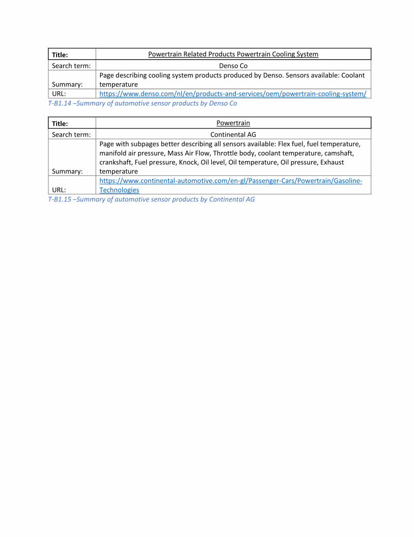
Title: Powertrain Related Products Powertrain Cooling System

Search term: Denso Co

Summary: Page describing cooling system products produced by Denso. Sensors available: Coolant temperature

URL: https://www.denso.com/nl/en/products-and-services/oem/powertrain-cooling-system/

T-B1.14 –Summary of automotive sensor products by Denso Co

Title: Powertrain

Search term: Continental AG

Summary:

Page with subpages better describing all sensors available: Flex fuel, fuel temperature, manifold air pressure, Mass Air Flow, Throttle body, coolant temperature, camshaft, crankshaft, Fuel pressure, Knock, Oil level, Oil temperature, Oil pressure, Exhaust temperature

URL: https://www.continental-automotive.com/en-gl/Passenger-Cars/Powertrain/Gasoline-Technologies

T-B1.15 –Summary of automotive sensor products by Continental AG

Appendix C Logbook and planning overview

Appendix E will consist of the project logbook maintained and the eventual planning overview in comparison to the initial planning. This section

of the appendix will contain of the following:

C1: Logbook

C2: Planning

C1 – Logbook Progression discussion per day per subject

22-Oct Task/Goal Description Relevant Information:

Morning Planning: Set out planning, hard due to wide research possibilities, determining what to achieve -

Afternoon Planning: Set out planning, hard due to wide research possibilities, determining what to achieve -

23-Oct Task/Goal Description Relevant Information:

Morning Planning: Finished Planning, reworked logbook in comparison to pre-research on topic, added clear tasks/goals -

Afternoon Sensor Research:

Got to about half of all automotive sensor manufacturers, collected information with summaries in an excel overview -

24-Oct Task/Goal Description Relevant Information:

Morning Sensor Research: Got to Bosch in list of sensor companies -

Afternoon

Sensor Research:

Finished sensor index for all major companies, most common sensors and availability now known -

Supervisor update:

Asked G.M. Stoffels if she would be willing to guide the thermodynamic modelling of the Internal combustion engine

-

Supervisor update:

Sent Email to A.J. Annema, R.N.J. Veldhuis, and G.J. Laanstra concerning setting the official start day at 22-october

-

Goal:

Decide on additional sensors to look into for potential research

-

25-Oct Task/Goal Description Relevant Information:

Morning Sensor Research: Looked into additional sensors, added them to sensor sheet and overview -

Afternoon

Sensor Research: Looked into additional sensors, added them to sensor sheet and overview -

Supervisor update:

Got a response from G.M. Stoffels, a meeting is planned for the 26th of October -

26-Oct Task/Goal Description Relevant Information:

Morning Sensor Research: Looked into next step and selection factors for sensors, sensor update speed, precision and signal potential seem good qualifiers -

Afternoon

Supervisor update:

Met with G.M. Stoffels, confirmed her as the third official examiner, she would be able to help on an intermediate basis, with a half an hour for questions where it would fit. Promised to go after concrete dates and deadlines for the presentation and report. -

Sensor Research:

Decided on sensor selection, Manifold Air Pressure will be the first, since it is always required in the model to determine airflow and is quicker than Mass Air Flow sensors.

See links Denso and Bosch for sensor research for speed of MAP and MAF (Appendix B)

29-Oct Task/Goal Description Relevant Information:

Morning Engine model: Sick, unfortunately no progression -

Afternoon

Supervisor meeting:

Sick, unfortunately missed meeting, setup new meeting for Friday 2 November with supervisors. -

Engine model: Sick, did manage to work on workings of model -

30-Oct Task/Goal Description Relevant Information:

Morning Engine model: Sick, unfortunately little progression -

Afternoon Engine model: Sick, unfortunately little progression -

31-Oct Task/Goal Description Relevant Information:

Morning Engine model:

Read in on thermodynamics, looked into venturi and diaphragms. Drew basic model of engine, realized quite the knowledge gap.

HyperPhysics

Wikipedia

Afternoon Engine model: Started on video lectures on Thermodynamics for more insight and a rough idea on where to start Khan Thermodynamics

01-Nov Task/Goal Description Relevant Information:

Morning Engine model: Read in on thermodynamics, piston problems, and combustion engine cycles -

Afternoon Engine model: Read in on thermodynamics, drew up another engine model, discussed with Mechanical Engineer brother on possible solutions -

02-Nov Task/Goal Description Relevant Information:

Morning

Engine model: Created pictures of preliminary model for progression presentation and interpretation -

Supervisor meeting preparation: Created presentation of meeting, as a summary of progression thus far -

Afternoon Supervisor meeting

Discussed deadlines, progression and current direction of research upon which was agreed. Also discussed meeting with G.M. Stoffels. -

05-Nov Task/Goal Description Relevant Information:

Morning Re-planning: Redoing the planning for concrete deadlines for ordering, model and measurement device -

Afternoon Re-planning: Done -

06-Nov Task/Goal Description Relevant Information:

Morning Test-engine: Looked at appropriate sensor locations, compared to online available sensors -

Afternoon Engine model: Determined required heat cycle steps for modelling of engine -

07-Nov Task/Goal Description Relevant Information:

Morning Engine model: Worked on implementation in MATLAB MATLAB engine model

Afternoon Engine model: Implemented piston velocity and translation model, including crankshaft offset, only time and resolution are to be added Piston model

08-Nov Task/Goal Description Relevant Information:

Morning

Engine model: Worked on implementation in MATLAB -

Sensor order: Figured out sensor types, sensors for which datasheets are available are more expensive, could it be paid by the University? -

Afternoon Sensor order: Found two good sensor options (MAP-T and EGT) and option via eBay, sent email to supervisors concerning ordering and cost NKG EGT

09-Nov Task/Goal Description Relevant Information:

Morning No progression: Was not able to work on model due to other appointments -

Afternoon No progression: Was not able to work on model due to other appointments -

12-Nov Task/Goal Description Relevant Information:

Morning Sensor order:

Response for supervisors, recommendation to check with European suppliers instead of part sites, also recommended to take a look at a scrapyard -

Afternoon Sensor implementation:

Got to work on exhaust manifold for EGT and Lambda sensors, tubing done. -

13-Nov Task/Goal Description Relevant Information:

Morning Sensor order: Called scrapyard, no response, will go there in person the 13th -

Afternoon Sensor implementation:

Finished exhaust manifold, sensor holes have to be tapped still, but will wait for actual sensors to confirm thread -

14-Nov Task/Goal Description Relevant Information:

Morning Engine model: Finished piston stroke/velocity model -

Afternoon

Sensor order:

Went to scrapyard, owner not present, left cell phone number. Did manage to get into the yard and determined available sensor brands mostly Denso and Bosch -

Sensor implementation:

Went on a search for the correct drill size for tapping, unfortunately it was not in stock. Got a wheel nut with correct hole diameter instead, which will be re-tapped -

15-Nov Task/Goal Description Relevant Information:

Morning Engine model: Clarified result plots to get better insight in model operation, through labels etc.. -

Afternoon

Presentation preparation:

Created piston stroke model result pictures, summarized sensor results, showed progression on exhaust manifold -

Sensor implementation:

Placed new exhaust manifold with lambda sensors under car, confirmed correct fitment -

16-Nov Task/Goal Description Relevant Information:

Morning Sensor order: Called scrapyard for information on EGT sensors, no BMW or Audi diesels available, so probably no EGT sensors available from yard -

Afternoon

Sensor order: Confirmed that order can be ordered by the University, order as quickly as possible -

Supervisor meeting:

Discussed progression, also got approved on decision to switch out model and measurement order, due to limited time until test-vehicle is not road legal. Sensors also agreed upon -

19-Nov Task/Goal Description Relevant Information:

Morning Sensor order:

Ordered 1 MAP sensor from Bosch, since it turned out that the sensor had a connector which could not easily be obtained. The cheap Chinese EGT sensor available in the Netherlands turned out to also have long delivery times, so an NGK EGT sensor was ordered. Also ordered corresponding connectors for sensors. -

Afternoon Sensor implementation: Created threaded weld in bung for EGT sensor -

20-Nov Task/Goal Description Relevant Information:

Morning Sensor order: Parts confirmed sent -

Afternoon Supervisor meeting

Went to G.M. Stoffels for signature on bachelor thesis form, discussed part of progression thus far -

21-Nov Task/Goal Description Relevant Information:

Morning Sensor implementation: Received sensors, welded in bung for EGT -

Afternoon

Engine model: Looked into Exhaust Gas Temperature model, got a better idea on how to model the process -

Sensor implementation:

Changed connector on EGT sensor, had a look at Arduino options for measurement. Found out that MAP connector was the same as ordered one, but 1 size larger in series. Determined another lambda sensor would be preferred with wired ground, since ground connection might be unreliable -

22-Nov Task/Goal Description Relevant Information:

Morning Sensor order:

Went to scrapyard, obtained Volvo 850 20v lambda sensor, same as current one, but with external ground wire for more reliable measurement. Also ordered a new exhaust gasket, an Arduino datalogger shield. -

Afternoon Sensor Implementation: Determined EGT sensor curve, and curve fit, did same for MAP sensor

NGK EGT

Bosch MAP

23-Nov Task/Goal Description Relevant Information:

Morning Sensor Implementation: Remounted exhaust with sensors in place, tested for exhaust leaks -

Afternoon Sensor Implementation:

Determined wiring lengths for sensors in car, measured coil signal to confirm suspicions of signal to detect, researched wheel speed sensors and air fuel ratio sensor read out

Wheel speed

Lambda/air-fuel

26-Nov Task/Goal Description Relevant Information:

Morning Sensor Implementation:

Drilled and tapped inlet manifold after removal, for addition of MAP/MAT sensor -

Afternoon Datalogger construction: Started datalogger box construction, including connectors -

Evening Sensor Implementation: Finished datalogger sensor loom -

27-Nov Task/Goal Description Relevant Information:

Morning Datalogger construction:

Started with circuit design, resistance measurement and input protection finished, put datalogger loom into test-vehicle and determined location for datalogger box -

Afternoon Datalogger construction:

Finished circuit design, pulse detection for wheel speed and engine speed now also included in the form of a Schmitt trigger Schmitt calculator

Evening Datalogger construction: Simulated all circuitry and confirmed correct operation -

28-Nov Task/Goal Description Relevant Information:

Morning Datalogger construction:

Added Neutrix connectors to datalogger enclosure, along with status led's, an Arduino Uno with the datalogger shield, and a circuit board for future operational amplifiers. Selected and simulated for mc3403 operational amplifiers (chosen for ability to get closer to rail), to assure new operational amplifiers selection will work -

Afternoon Datalogger construction:

Soldered all circuits and debugged the circuit. Figured out several issues with ignition pulse detector, redid the simulation to resolve, implemented and tested design once more -

Evening Datalogger construction:

Mounted datalogger in test-vehicle, attempted first test drive. Arduino power supply turned out to be failing, as shown by status leds, repairs will be attempted next day. -

29-Nov Task/Goal Description Relevant Information:

Morning Datalogger construction:

Datalogger ended up being wired wrongly, which was repaired. Arduino was reprogrammed, however it would not communicate, so new Arduino chip was used. Serial communication worked once more, so test drive was initiated, due to wiring issues Arduino power regulator got damaged and a new Arduino board was required and installed. -

Afternoon Datalogger construction:

In order to prevent future damage LM7805 voltage regulator was added for bigger input voltage swing tolerance, and the Arduino was now fed 5v through the fused usb port. -

Evening Datalogger construction:

Reprogrammed Arduino and prepped for new test drive, datalogger now operational, ready for measurement -

30-Nov Task/Goal Description Relevant Information:

Morning Measurements: Drove to ice track with large open parking space, cleared datalogger SD card and finished wide open throttle and constant rpm tests -

Afternoon Measurements:

Drove to Hengelo and back over an 80 km/h section, in 3,4,5 gear with constant rpm for varying load test. Also did 0-60km/h runs in second gear for (1000 to 5000) rpm, and let car roll to 1000 rpm again, for friction determination, however forgot to press clutch so these results are less useful for rolling friction determination. -

Evening Measurements: Created log of attempted measurements, with notes taken during data logged runs -

03-Dec Task/Goal Description Relevant Information:

Morning

Presentation preparation:

Prepared progression presentation, with datalogger construction and measurements as they now sat. -

Supervisor meeting:

Discussed datalogger electronics, measurement runs with idea behind them, and showed measurement data as far as I got. Got improvement tips concerning operational amplifiers selection and use of ADC range on Arduino, concerning rail to rail operational amplifiers, which I will consider in the next project of the sort. -

Afternoon

Planning: Revised planning once more, added corrected deadlines in agenda -

Measurement analysis:

Had a look at the measurement data, created scraper for reading in and applying correction curves to data. Since rpm signal appears unreliable, hopefully MAP signal will allow for better rpm representation -

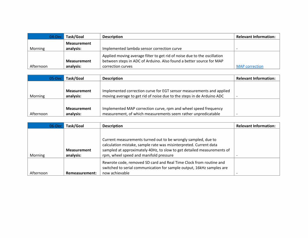
04-Dec Task/Goal Description Relevant Information:

Morning Measurement analysis: Implemented lambda sensor correction curve -

Afternoon Measurement analysis:

Applied moving average filter to get rid of noise due to the oscillation between steps in ADC of Arduino. Also found a better source for MAP correction curves MAP correction

05-Dec Task/Goal Description Relevant Information:

Morning Measurement analysis:

Implemented correction curve for EGT sensor measurements and applied moving average to get rid of noise due to the steps in de Arduino ADC -

Afternoon Measurement analysis:

Implemented MAP correction curve, rpm and wheel speed frequency measurement, of which measurements seem rather unpredicatable -

06-Dec Task/Goal Description Relevant Information:

Morning Measurement analysis:

Current measurements turned out to be wrongly sampled, due to calculation mistake, sample rate was misinterpreted. Current data sampled at approximately 40Hz, to slow to get detailed measurements of rpm, wheel speed and manifold pressure -

Afternoon Remeasurement:

Rewrote code, removed SD card and Real Time Clock from routine and switched to serial communication for sample output, 16kHz samples are now achievable -

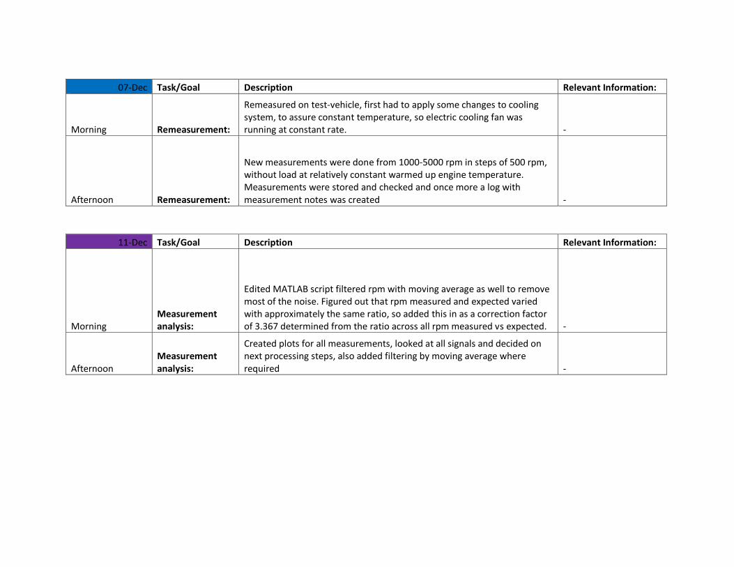
07-Dec Task/Goal Description Relevant Information:

Morning Remeasurement:

Remeasured on test-vehicle, first had to apply some changes to cooling system, to assure constant temperature, so electric cooling fan was running at constant rate. -

Afternoon Remeasurement:

New measurements were done from 1000-5000 rpm in steps of 500 rpm, without load at relatively constant warmed up engine temperature. Measurements were stored and checked and once more a log with measurement notes was created -

11-Dec Task/Goal Description Relevant Information:

Morning Measurement analysis:

Edited MATLAB script filtered rpm with moving average as well to remove most of the noise. Figured out that rpm measured and expected varied with approximately the same ratio, so added this in as a correction factor of 3.367 determined from the ratio across all rpm measured vs expected. -

Afternoon Measurement analysis:

Created plots for all measurements, looked at all signals and decided on next processing steps, also added filtering by moving average where required -

12-Dec Task/Goal Description Relevant Information:

Morning Measurement analysis:

Compared manifold pressure signal with expected rpm pulses, same shape but incorrect timing? -

Afternoon Measurement analysis:

Reinterpreted results, problem figured out, in measurement script timing function did not consider serial communication write time, correction factor for rpm, is measure of actual delta time's, applied correction factor to time scale, results now align with provided source MAP measurement

13-Dec Task/Goal Description Relevant Information:

Morning Engine model:

Researched flow op poppet valves as found in test engine, found it to be generally very complex, shrouding causes many issues as shown in linked paper, requires simplification Poppet valve paper

Afternoon Engine model:

Assumed piston speed is equal to air flow speed, with effective area the flow can then be determined. Found a source for poppet valve estimated effective area based on discharge coefficient Cd = 0.6 Valve flow

14-Dec Task/Goal Description Relevant Information:

Morning Engine model: Added intake flow to model, also determined parabola for lift curves of camshaft (see link), and added these estimates to model Camshaft in car

Afternoon Engine model: Worked on camshaft model, flow now based on lift, and confirmed to be correct for all angles -

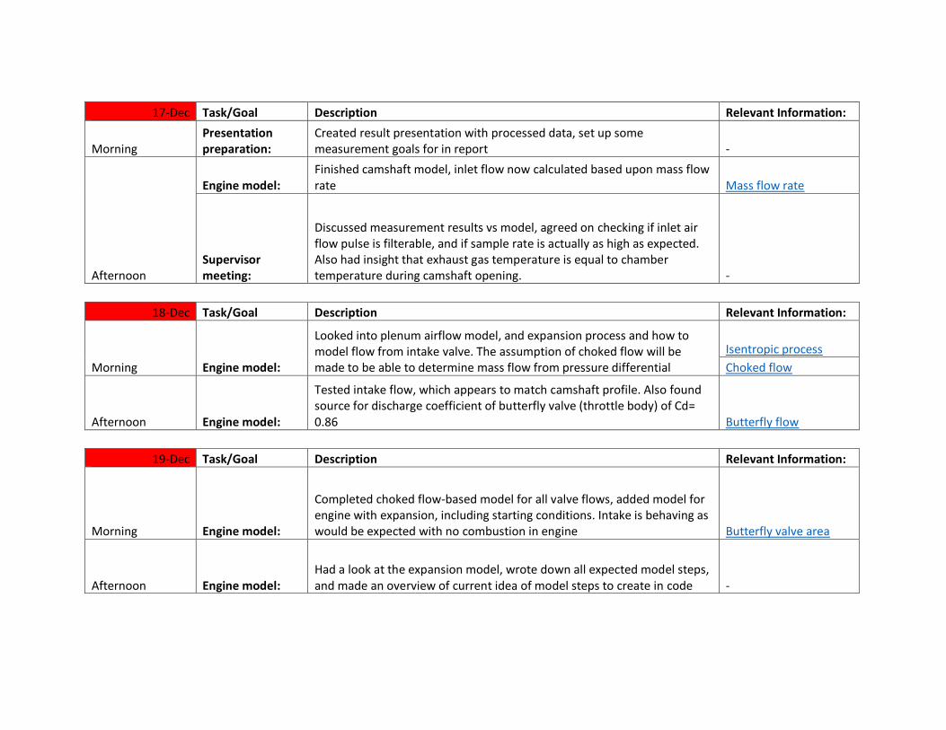
17-Dec Task/Goal Description Relevant Information:

Morning Presentation preparation:

Created result presentation with processed data, set up some measurement goals for in report -

Afternoon

Engine model: Finished camshaft model, inlet flow now calculated based upon mass flow rate Mass flow rate

Supervisor meeting:

Discussed measurement results vs model, agreed on checking if inlet air flow pulse is filterable, and if sample rate is actually as high as expected. Also had insight that exhaust gas temperature is equal to chamber temperature during camshaft opening. -

18-Dec Task/Goal Description Relevant Information:

Morning Engine model:

Looked into plenum airflow model, and expansion process and how to model flow from intake valve. The assumption of choked flow will be made to be able to determine mass flow from pressure differential

Isentropic process

Choked flow

Afternoon Engine model:

Tested intake flow, which appears to match camshaft profile. Also found source for discharge coefficient of butterfly valve (throttle body) of Cd= 0.86 Butterfly flow

19-Dec Task/Goal Description Relevant Information:

Morning Engine model:

Completed choked flow-based model for all valve flows, added model for engine with expansion, including starting conditions. Intake is behaving as would be expected with no combustion in engine Butterfly valve area

Afternoon Engine model: Had a look at the expansion model, wrote down all expected model steps, and made an overview of current idea of model steps to create in code -

20-Dec Task/Goal Description Relevant Information:

Morning

Engine model: Implemented correction curve for specific heats of dry air for exhaust gas and expansion model Dry air properties

Supervisor: Asked G.M. Stoffels if I could set up a meeting to discuss model assumptions -

Afternoon Supervisor meeting:

Met with G.M. Stoffels to discuss model assumptions, no strange things were found, should work as expected -

21-Dec Task/Goal Description Relevant Information:

Morning Engine model:

Debugged model, switched some calculations and variables, resulting in non-real values. Also moved piston and mass flow model out of main model, for better overview of calculation steps -

Afternoon Engine model: First model results, shape of manifold pressure appears to align with measured manifold pressure for 1000 rpm -

22-Dec Task/Goal Description Relevant Information:

Morning Engine model:

Oscillations are observed for exhaust flow in model, which got worse with shorter timesteps. Changed order of model calculation steps, oscillation is less but not yet gone. Will have to look into pressure calculations -

Afternoon Engine model:

Added temperature to combustion chamber at TDC after intake stroke, to model combustion as instantaneous addition of energy. Determined temperature of chamber as well, temperature appears to drop below zero resulting, something is off in the mass flow calculation. -

23-Dec Task/Goal Description Relevant Information:

Morning Engine model: Looked into chamber temperature some more, changed calculation order around, also checked mass flow calculation, still no solution to problem -

Afternoon Engine model: Mistake found in timestep calculation, less oscillation observed, and temperature overshoot now constant, and not getting more negative. -

24-Dec Task/Goal Description Relevant Information:

Morning Engine model: Reworked plots to hopefully get more insight into where the model is failing -

Afternoon Engine model: Still cannot figure out issue with model -

25-Dec Task/Goal Description Relevant Information:

Morning Measurement Analysis:

Finished measurement scraper and started selecting sections of measured engine operating conditions to save and to take an fft of. Long sections of 5 seconds with relatively constant rpm and short sections of 5 manifold air pressure pulses were chosen, along with an overview of the whole measurement run -

Afternoon Measurement Analysis:

Reworked output format, added frequency markers to fft, added correct labels, added average value line with value where required -

26-Dec Task/Goal Description Relevant Information:

Morning Engine model:

Found out issue with temperature, model should be based on energy per unit mass, and then temperature should follow from specific heat properties. Started on reworking model to work with delta mass and delta Q (energy) -

Afternoon Engine model: Finished reworking expansion and flow steps, still need to add combustion process -

27-Dec Task/Goal Description Relevant Information:

Morning Engine model: Added combustion as a function of lambda and energy in petrol, all petrol added is assumed to burn with a stoic mixture -

Afternoon Engine model: Model now appears to work correctly, also removed correction factor for flow, since it was only required for testing of flow issue -

28-Dec Task/Goal Description Relevant Information:

Morning Measurement Analysis: Started storing measurement sections plots -

Afternoon Measurement Analysis: Finished storing measurement section plots -

30-Dec Task/Goal Description Relevant Information:

Morning Engine model: Rewrote model plots to match measurement plots, to more easily compare results, also added labels and average values -

Afternoon Engine model:

Also added FFT with peaks, and created camshaft zero and peak moment identifiers for both intake and exhaust valves for comparison to manifold air pressure pulse -

31-Dec Task/Goal Description Relevant Information:

Morning Engine model: Attempted to start storing model comparison results for actual measurements, ran in to issues with values running to infinity -

Afternoon Engine model:

Looked into all calculation steps, minor issues resolved. Discovered issue with timestep when Ddegrees (resolution of simulation) was changed, calculation does not seem correct. Did manage to add all cylinders for modelled b230k engine in correct offset. -

01-Jan Task/Goal Description Relevant Information:

Morning Engine model: Rewrote manner in which timestep is calculated. -

Afternoon Engine model:

With new timestep plot results had to be reconfigured to align correctly, now everything seems correct except for manifold temperature, will have a think about an explanation, but for now it is time to start on the report, since it is long overdue. Created layout for rapport with correct chapters and appendices -

02-Jan Task/Goal Description Relevant Information:

Morning Model Results:

Got to work on matching al measurements to a suitable model run, sections of 4 manifold pressure peaks, and sections of 10 engine rotations were used for comparison -

Afternoon Report:

Got to work on Appendix B containing all research concerning automotive sensors and Appendix A containing the engine modelling research collected -

Evening Report: Got to work on Appendix E containing correction curves for all sensors and the heat capacities of dry air -

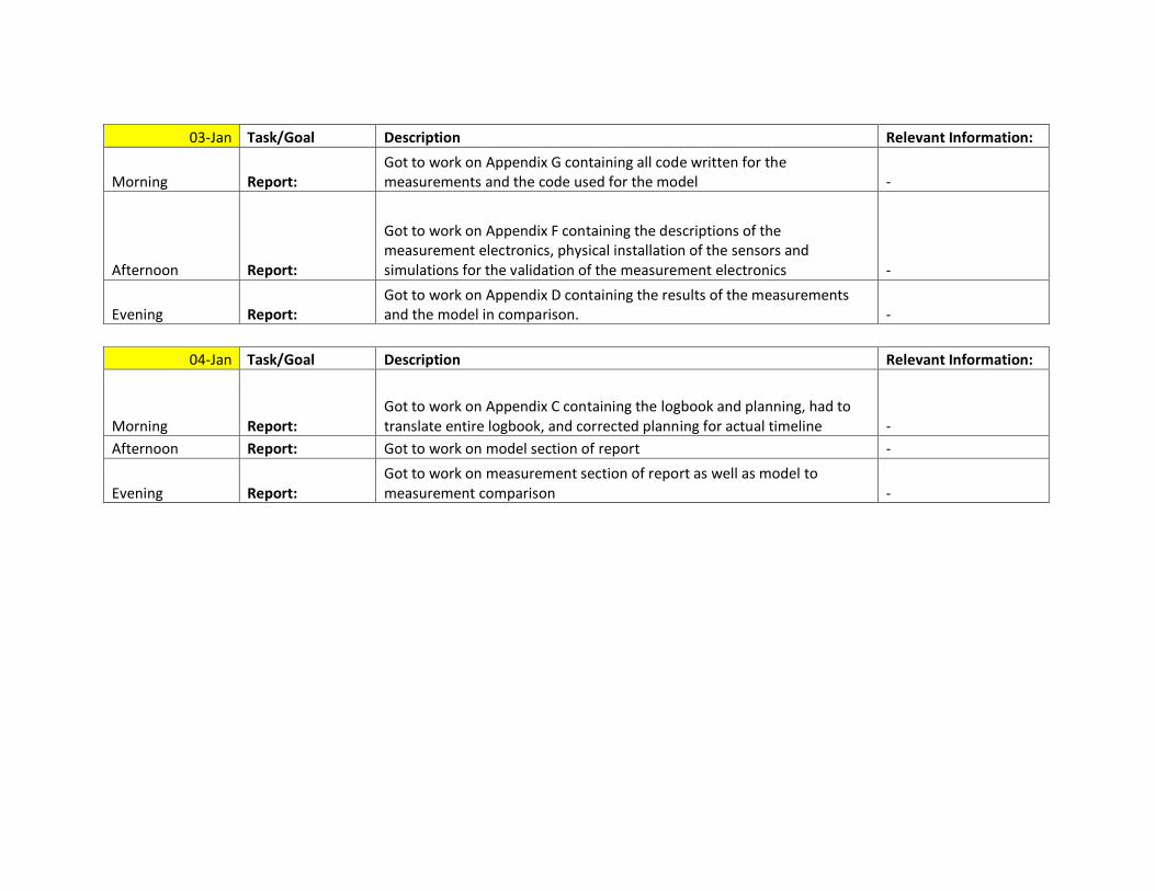
03-Jan Task/Goal Description Relevant Information:

Morning Report: Got to work on Appendix G containing all code written for the measurements and the code used for the model -

Afternoon Report:

Got to work on Appendix F containing the descriptions of the measurement electronics, physical installation of the sensors and simulations for the validation of the measurement electronics -

Evening Report: Got to work on Appendix D containing the results of the measurements and the model in comparison. -

04-Jan Task/Goal Description Relevant Information:

Morning Report: Got to work on Appendix C containing the logbook and planning, had to translate entire logbook, and corrected planning for actual timeline -

Afternoon Report: Got to work on model section of report -

Evening Report: Got to work on measurement section of report as well as model to measurement comparison -

C2 – Initial planning overview Planning estimate at start of project

Week, Day 22-Oct 23-Oct 24-Oct 25-Oct 26-Oct 29-Oct 30-Oct 31-Oct 01-Nov 02-Nov 05-Nov 06-Nov 07-Nov 08-Nov 09-NovLiterature research> Available/common sensors> Current readout methodologies> Estimation of possibilities

Focus study> Sensor selection> Goal of improvement> Expected measurement model

Measurement device> Basic design, ordering of sensors> Construction + implementation

Measurements> Measurement plan> Actual measurement> Measurement checks

Analysis> Signal cleanup> Model comparison> Conclusions

Report writing #1> Research> Model> Measurement

Report writing #2> Results/conclusions> Sources> Images etc

Report Repair> Results/conclusions> Sources> Improve with feedback

Presentation preparation> Prepare presentation> Presentation

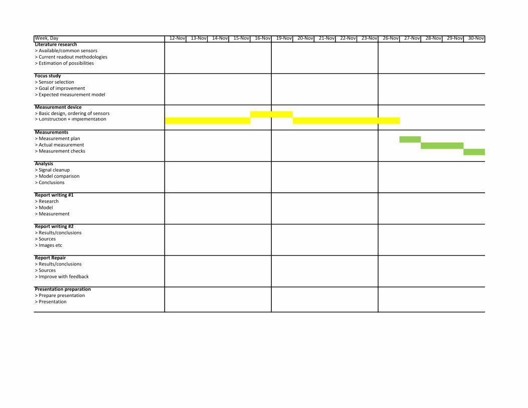
Week, Day 12-Nov 13-Nov 14-Nov 15-Nov 16-Nov 19-Nov 20-Nov 21-Nov 22-Nov 23-Nov 26-Nov 27-Nov 28-Nov 29-Nov 30-NovLiterature research> Available/common sensors> Current readout methodologies> Estimation of possibilities

Focus study> Sensor selection> Goal of improvement> Expected measurement model

Measurement device> Basic design, ordering of sensors> Construction + implementation

Measurements> Measurement plan> Actual measurement> Measurement checks

Analysis> Signal cleanup> Model comparison> Conclusions

Report writing #1> Research> Model> Measurement

Report writing #2> Results/conclusions> Sources> Images etc

Report Repair> Results/conclusions> Sources> Improve with feedback

Presentation preparation> Prepare presentation> Presentation

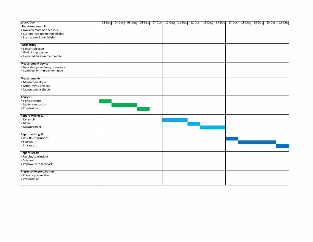
Week, Day 03-Dec 04-Dec 05-Dec 06-Dec 07-Dec 10-Dec 11-Dec 12-Dec 13-Dec 14-Dec 17-Dec 18-Dec 19-Dec 20-Dec 21-DecLiterature research> Available/common sensors> Current readout methodologies> Estimation of possibilities

Focus study> Sensor selection> Goal of improvement> Expected measurement model

Measurement device> Basic design, ordering of sensors> Construction + implementation

Measurements> Measurement plan> Actual measurement> Measurement checks

Analysis> Signal cleanup> Model comparison> Conclusions

Report writing #1> Research> Model> Measurement

Report writing #2> Results/conclusions> Sources> Images etc

Report Repair> Results/conclusions> Sources> Improve with feedback

Presentation preparation> Prepare presentation> Presentation

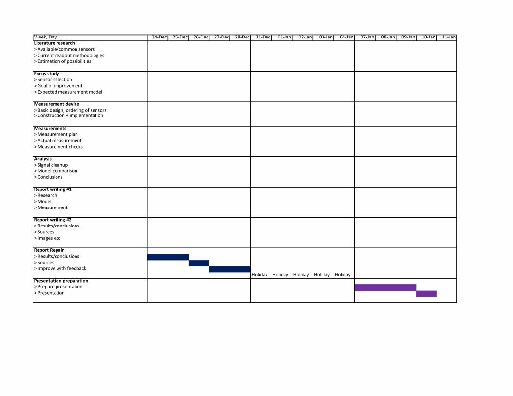
Week, Day 24-Dec 25-Dec 26-Dec 27-Dec 28-Dec 31-Dec 01-Jan 02-Jan 03-Jan 04-Jan 07-Jan 08-Jan 09-Jan 10-Jan 11-JanLiterature research> Available/common sensors> Current readout methodologies> Estimation of possibilities

Focus study> Sensor selection> Goal of improvement> Expected measurement model

Measurement device> Basic design, ordering of sensors> Construction + implementation

Measurements> Measurement plan> Actual measurement> Measurement checks

Analysis> Signal cleanup> Model comparison> Conclusions

Report writing #1> Research> Model> Measurement

Report writing #2> Results/conclusions> Sources> Images etc

Report Repair> Results/conclusions> Sources> Improve with feedback

Holiday Holiday Holiday Holiday HolidayPresentation preparation> Prepare presentation> Presentation

Appendix D Measurement and model results in comparison

Appendix D will consist of all measurements and model runs for these measurements, sorted by engine speed in

revolutions per minute (rpm). It has been structured as follows:

D1: Measurements and simulation results for 1000 rpm

D2: Measurements and simulation results for 1500 rpm

D3: Measurements and simulation results for 2000 rpm

D4: Measurements and simulation results for 2500 rpm

D5: Measurements and simulation results for 3000 rpm

D6: Measurements and simulation results for 3500 rpm

D7: Measurements and simulation results for 4000 rpm

D8: Measurements and simulation results for 4500 rpm

D9: Measurements and simulation results for 5000 rpm

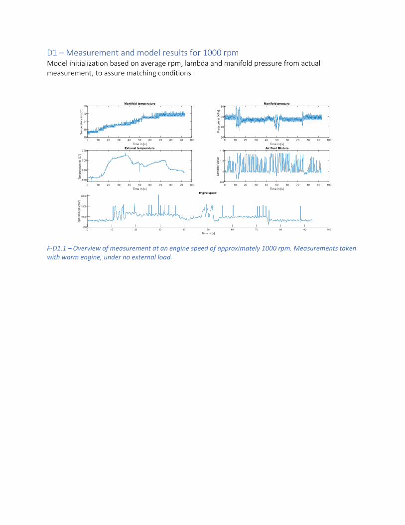
D1 – Measurement and model results for 1000 rpm Model initialization based on average rpm, lambda and manifold pressure from actual measurement, to assure matching conditions.

F-D1.1 – Overview of measurement at an engine speed of approximately 1000 rpm. Measurements taken with warm engine, under no external load.

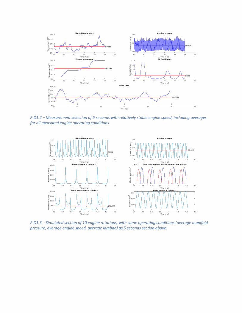
F-D1.2 – Measurement selection of 5 seconds with relatively stable engine speed, including averages for all measured engine operating conditions.

F-D1.3 – Simulated section of 10 engine rotations, with same operating conditions (average manifold pressure, average engine speed, average lambda) as 5 seconds section above.

F-D1.4 – Fast Fourier transform for measurement selection of 5 seconds with relatively stable engine speed, including averages for all measured engine operating conditions.

F-D1.5 – Fast Fourier transform for simulated section of 10 engine rotations, with same operating conditions (average manifold pressure, average engine speed, average lambda) as 5 seconds section above.

F-D1.6 – Measurement selection of 5 pressure peaks with relatively stable engine speed and lambda value, including averages for all measured engine operating conditions.

F-D1.7 – Simulated section of 4 pressure peaks, with same operating conditions (average manifold pressure, average engine speed, average lambda) as 5 peak section above.

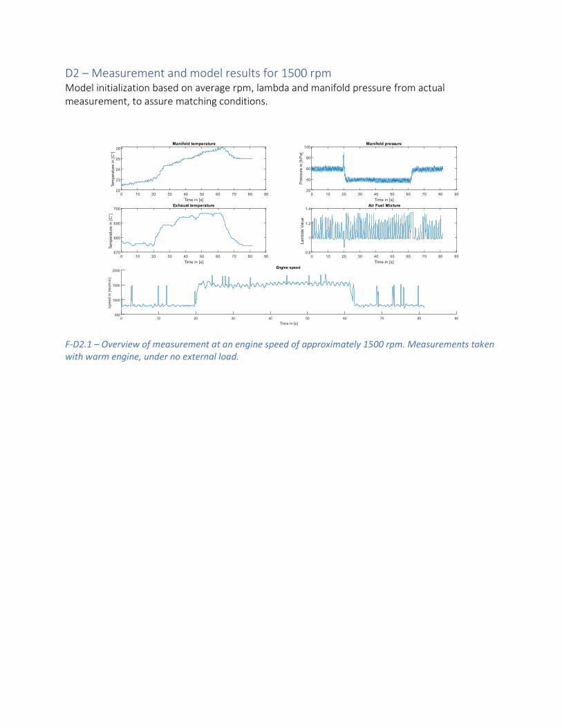
D2 – Measurement and model results for 1500 rpm Model initialization based on average rpm, lambda and manifold pressure from actual measurement, to assure matching conditions.

F-D2.1 – Overview of measurement at an engine speed of approximately 1500 rpm. Measurements taken with warm engine, under no external load.

F-D2.2 – Measurement selection of 5 seconds with relatively stable engine speed, including averages for all measured engine operating conditions.

F-D2.3 – Simulated section of 10 engine rotations, with same operating conditions (average manifold pressure, average engine speed, average lambda) as 5 seconds section above.

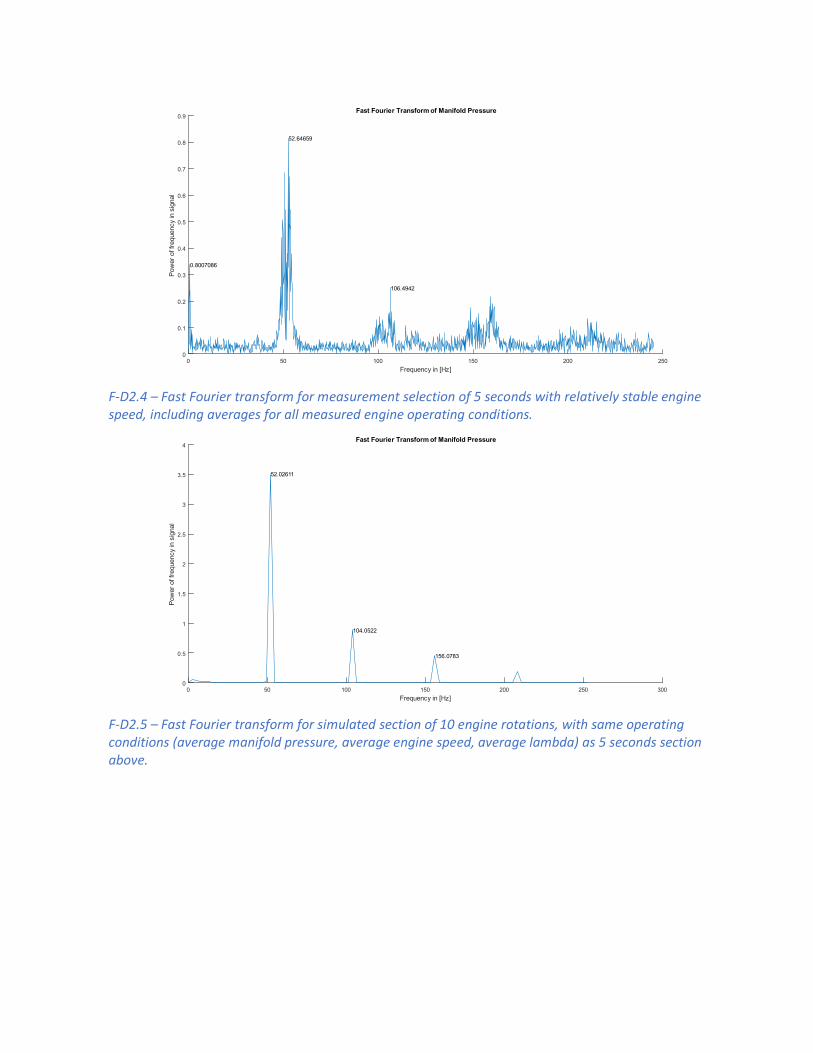
F-D2.4 – Fast Fourier transform for measurement selection of 5 seconds with relatively stable engine speed, including averages for all measured engine operating conditions.

F-D2.5 – Fast Fourier transform for simulated section of 10 engine rotations, with same operating conditions (average manifold pressure, average engine speed, average lambda) as 5 seconds section above.

F-D2.6 – Measurement selection of 5 pressure peaks with relatively stable engine speed and lambda value, including averages for all measured engine operating conditions.

F-D2.7 – Simulated section of 4 pressure peaks, with same operating conditions (average manifold pressure, average engine speed, average lambda) as 5 peak section above.

D3 – Measurement and model results for 2000 rpm Model initialization based on average rpm, lambda and manifold pressure from actual measurement, to assure matching conditions.

F-D3.1 – Overview of measurement at an engine speed of approximately 2000 rpm. Measurements taken with warm engine, under no external load.

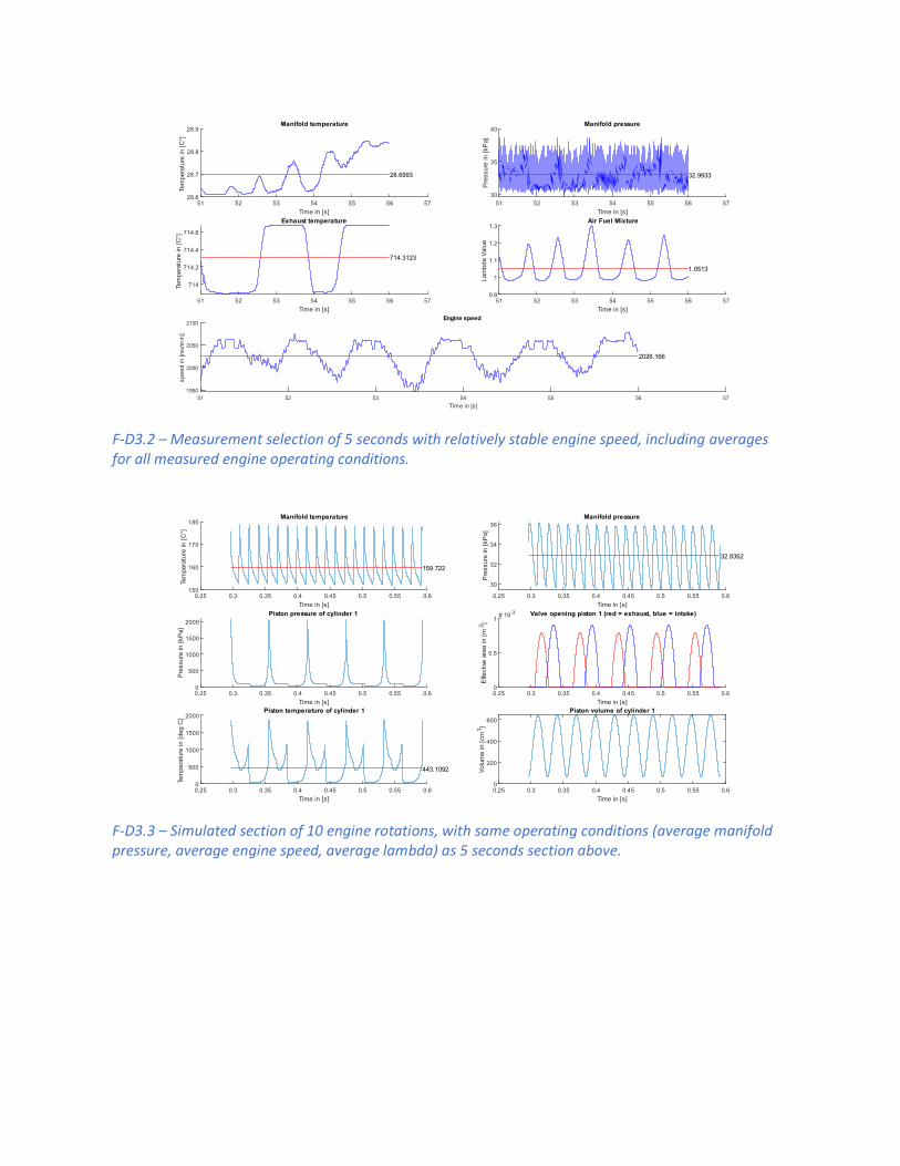
F-D3.2 – Measurement selection of 5 seconds with relatively stable engine speed, including averages for all measured engine operating conditions.

F-D3.3 – Simulated section of 10 engine rotations, with same operating conditions (average manifold pressure, average engine speed, average lambda) as 5 seconds section above.

F-D3.4 – Fast Fourier transform for measurement selection of 5 seconds with relatively stable engine speed, including averages for all measured engine operating conditions.

F-D3.5 – Fast Fourier transform for simulated section of 10 engine rotations, with same operating conditions (average manifold pressure, average engine speed, average lambda) as 5 seconds section above.

F-D3.6 – Measurement selection of 5 pressure peaks with relatively stable engine speed and lambda value, including averages for all measured engine operating conditions.

F-D3.7 – Simulated section of 4 pressure peaks, with same operating conditions (average manifold pressure, average engine speed, average lambda) as 5 peak section above.

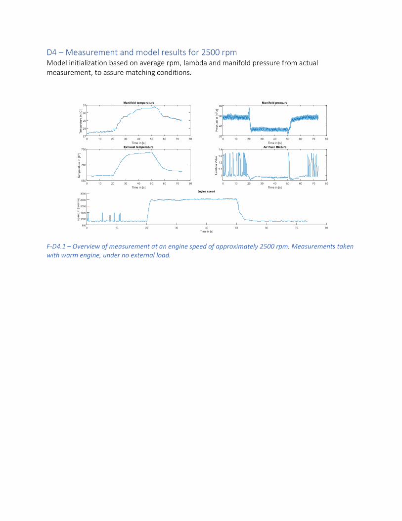
D4 – Measurement and model results for 2500 rpm Model initialization based on average rpm, lambda and manifold pressure from actual measurement, to assure matching conditions.

F-D4.1 – Overview of measurement at an engine speed of approximately 2500 rpm. Measurements taken with warm engine, under no external load.

F-D4.2 – Measurement selection of 5 seconds with relatively stable engine speed, including averages for all measured engine operating conditions.

F-D4.3 – Simulated section of 10 engine rotations, with same operating conditions (average manifold pressure, average engine speed, average lambda) as 5 seconds section above.

F-D4.4 – Fast Fourier transform for measurement selection of 5 seconds with relatively stable engine speed, including averages for all measured engine operating conditions.

F-D4.5 – Fast Fourier transform for simulated section of 10 engine rotations, with same operating conditions (average manifold pressure, average engine speed, average lambda) as 5 seconds section above.

F-D4.6 – Measurement selection of 5 pressure peaks with relatively stable engine speed and lambda value, including averages for all measured engine operating conditions.

F-D4.7 – Simulated section of 4 pressure peaks, with same operating conditions (average manifold pressure, average engine speed, average lambda) as 5 peak section above.

D5 – Measurement and model results for 3000 rpm Model initialization based on average rpm, lambda and manifold pressure from actual measurement, to assure matching conditions.

F-D5.1 – Overview of measurement at an engine speed of approximately 3000 rpm. Measurements taken with warm engine, under no external load.

F-D5.2 – Measurement selection of 5 seconds with relatively stable engine speed, including averages for all measured engine operating conditions.

F-D5.3 – Simulated section of 10 engine rotations, with same operating conditions (average manifold pressure, average engine speed, average lambda) as 5 seconds section above.

F-D5.4 – Fast Fourier transform for measurement selection of 5 seconds with relatively stable engine speed, including averages for all measured engine operating conditions.

F-D5.5 – Fast Fourier transform for simulated section of 10 engine rotations, with same operating conditions (average manifold pressure, average engine speed, average lambda) as 5 seconds section above.

F-D5.6 – Measurement selection of 5 pressure peaks with relatively stable engine speed and lambda value, including averages for all measured engine operating conditions.

F-D5.7 – Simulated section of 4 pressure peaks, with same operating conditions (average manifold pressure, average engine speed, average lambda) as 5 peak section above.

D6 – Measurement and model results for 3500 rpm Model initialization based on average rpm, lambda and manifold pressure from actual measurement, to assure matching conditions.

F-D6.1 – Overview of measurement at an engine speed of approximately 3500 rpm. Measurements taken with warm engine, under no external load.

F-D6.2 – Measurement selection of 5 seconds with relatively stable engine speed, including averages for all measured engine operating conditions.

F-D6.3 – Simulated section of 10 engine rotations, with same operating conditions (average manifold pressure, average engine speed, average lambda) as 5 seconds section above.

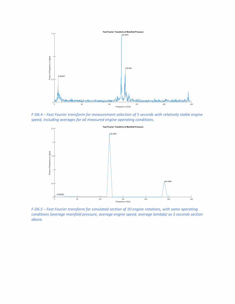
F-D6.4 – Fast Fourier transform for measurement selection of 5 seconds with relatively stable engine speed, including averages for all measured engine operating conditions.

F-D6.5 – Fast Fourier transform for simulated section of 10 engine rotations, with same operating conditions (average manifold pressure, average engine speed, average lambda) as 5 seconds section above.

F-D6.6 – Measurement selection of 5 pressure peaks with relatively stable engine speed and lambda value, including averages for all measured engine operating conditions.

F-D6.7 – Simulated section of 4 pressure peaks, with same operating conditions (average manifold pressure, average engine speed, average lambda) as 5 peak section above.

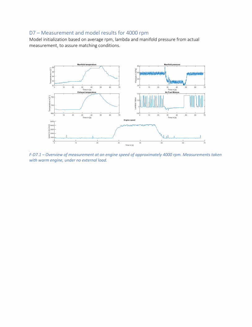
D7 – Measurement and model results for 4000 rpm Model initialization based on average rpm, lambda and manifold pressure from actual measurement, to assure matching conditions.

F-D7.1 – Overview of measurement at an engine speed of approximately 4000 rpm. Measurements taken with warm engine, under no external load.

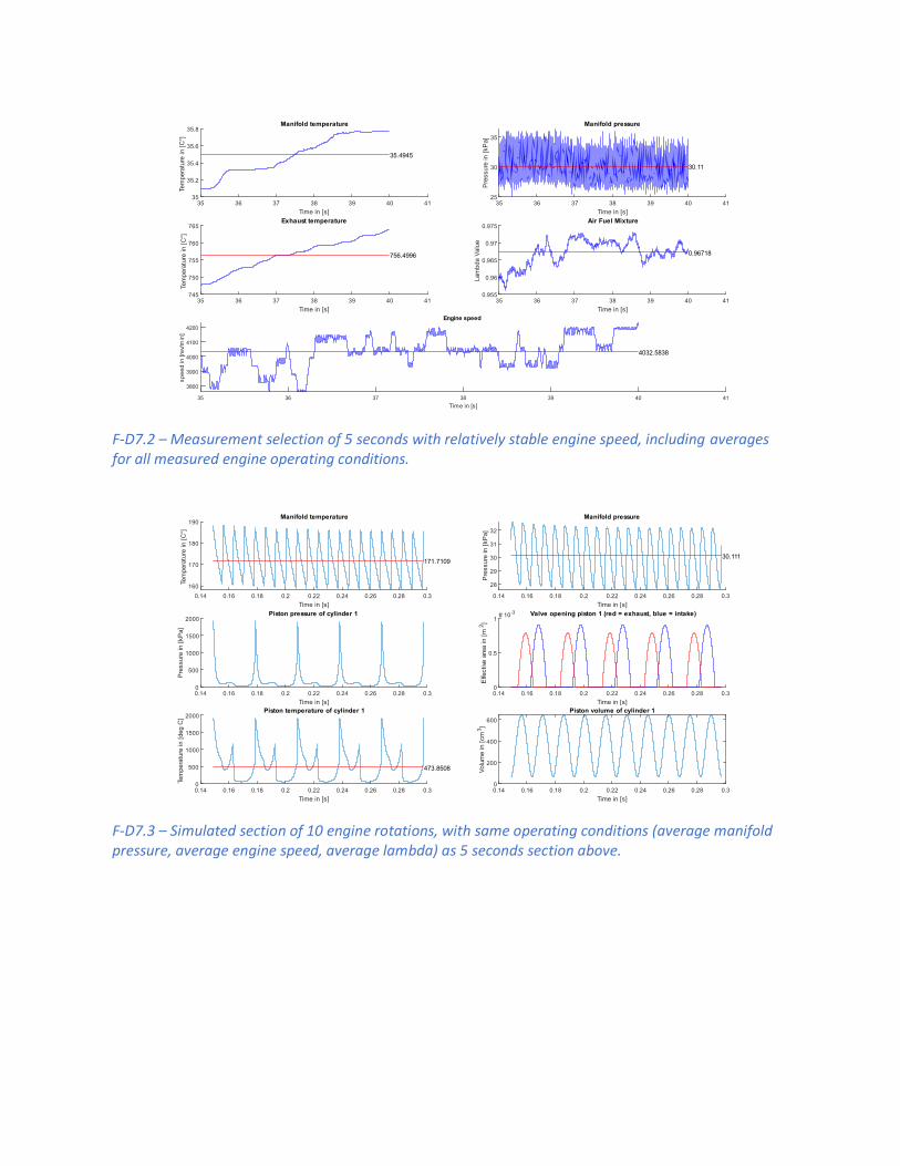
F-D7.2 – Measurement selection of 5 seconds with relatively stable engine speed, including averages for all measured engine operating conditions.

F-D7.3 – Simulated section of 10 engine rotations, with same operating conditions (average manifold pressure, average engine speed, average lambda) as 5 seconds section above.

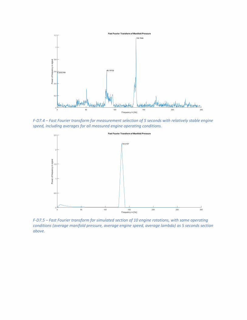
F-D7.4 – Fast Fourier transform for measurement selection of 5 seconds with relatively stable engine speed, including averages for all measured engine operating conditions.

F-D7.5 – Fast Fourier transform for simulated section of 10 engine rotations, with same operating conditions (average manifold pressure, average engine speed, average lambda) as 5 seconds section above.

F-D7.6 – Measurement selection of 5 pressure peaks with relatively stable engine speed and lambda value, including averages for all measured engine operating conditions.

F-D7.7 – Simulated section of 4 pressure peaks, with same operating conditions (average manifold pressure, average engine speed, average lambda) as 5 peak section above.

D8 – Measurement and model results for 4500 rpm Model initialization based on average rpm, lambda and manifold pressure from actual measurement, to assure matching conditions.

F-D8.1 – Overview of measurement at an engine speed of approximately 4500 rpm. Measurements taken with warm engine, under no external load.

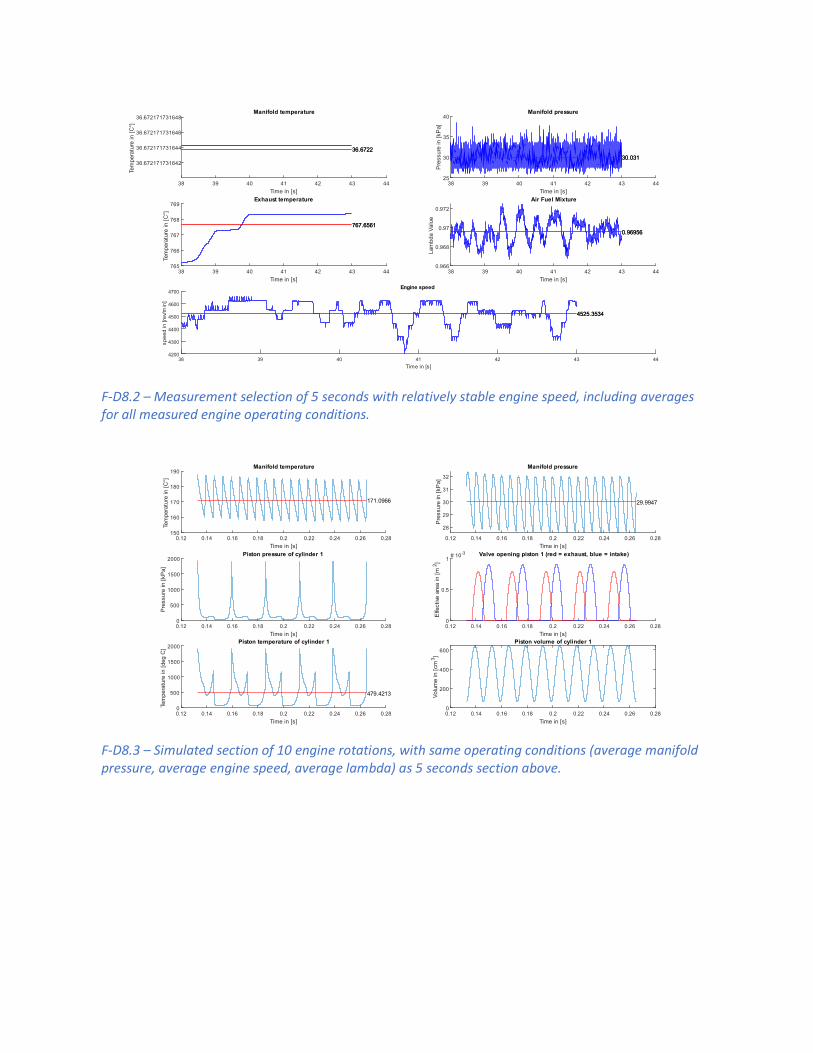
F-D8.2 – Measurement selection of 5 seconds with relatively stable engine speed, including averages for all measured engine operating conditions.

F-D8.3 – Simulated section of 10 engine rotations, with same operating conditions (average manifold pressure, average engine speed, average lambda) as 5 seconds section above.

F-D8.4 – Fast Fourier transform for measurement selection of 5 seconds with relatively stable engine speed, including averages for all measured engine operating conditions.

F-D8.5 – Fast Fourier transform for simulated section of 10 engine rotations, with same operating conditions (average manifold pressure, average engine speed, average lambda) as 5 seconds section above.

F-D8.6 – Measurement selection of 5 pressure peaks with relatively stable engine speed and lambda value, including averages for all measured engine operating conditions.

F-D8.7 – Simulated section of 4 pressure peaks, with same operating conditions (average manifold pressure, average engine speed, average lambda) as 5 peak section above.

D9 – Measurement and model results for 5000 rpm Model initialization based on average rpm, lambda and manifold pressure from actual measurement, to assure matching conditions.

F-D9.1 – Overview of measurement at an engine speed of approximately 5000 rpm. Measurements taken with warm engine, under no external load.

F-D9.2 – Measurement selection of 5 seconds with relatively stable engine speed, including averages for all measured engine operating conditions.

F-D9.3 – Simulated section of 10 engine rotations, with same operating conditions (average manifold pressure, average engine speed, average lambda) as 5 seconds section above.

F-D9.4 – Fast Fourier transform for measurement selection of 5 seconds with relatively stable engine speed, including averages for all measured engine operating conditions.

F-D9.5 – Fast Fourier transform for simulated section of 10 engine rotations, with same operating conditions (average manifold pressure, average engine speed, average lambda) as 5 seconds section above.

F-D9.6 – Measurement selection of 5 pressure peaks with relatively stable engine speed and lambda value, including averages for all measured engine operating conditions.

F-D9.7 – Simulated section of 4 pressure peaks, with same operating conditions (average manifold pressure, average engine speed, average lambda) as 5 peak section above.

Appendix E Sensor calibration curves and their sources

Appendix E will consist of all calibration and estimate curves used for sensor translation and model

parameters, that are dependent in some manner upon other variables. This section of the appendix will

contain of the following:

E1: Estimate curve for constant volume specific heat (cv) of dry air

E2: Estimate curve for specific heat ratio (γ) of dry air

E3: Estimated Resistance curve of Exhaust Gas Temperature sensor (EGT)

E4: Estimated Resistance curve of Manifold Air Temperature sensor (MAT)

E5: Estimated Voltage curve of Manifold Air Pressure sensor (MAP)

E6: Estimated Voltage curve Narrowband Air-Fuel ratio sensor (LAMBDA)

E7: Estimated Camshaft profiles for used Volvo b230k test engine

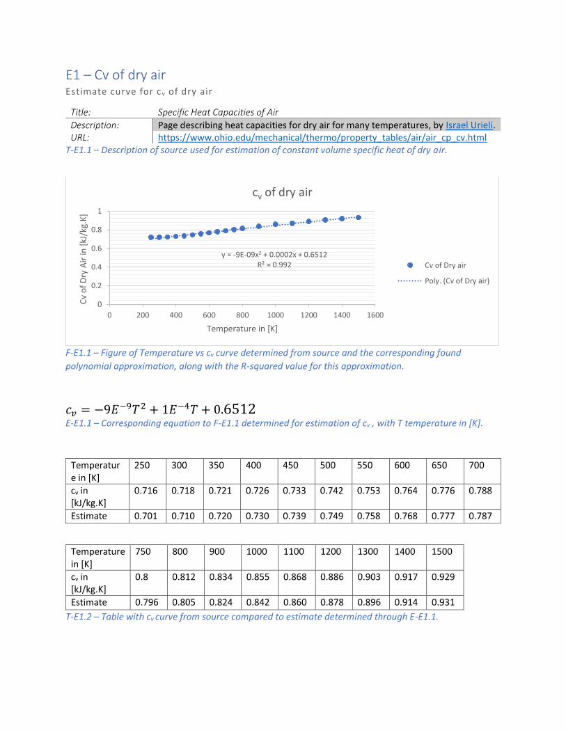
E1 – Cv of dry air Estimate curve for c v of dry air

Title: Specific Heat Capacities of Air

Description: Page describing heat capacities for dry air for many temperatures, by Israel Urieli. URL: https://www.ohio.edu/mechanical/thermo/property_tables/air/air_cp_cv.html

T-E1.1 – Description of source used for estimation of constant volume specific heat of dry air.

F-E1.1 – Figure of Temperature vs cv curve determined from source and the corresponding found

polynomial approximation, along with the R-squared value for this approximation.

𝑐𝑣 = −9𝐸−9𝑇2 + 1𝐸−4𝑇 + 0.6512 E-E1.1 – Corresponding equation to F-E1.1 determined for estimation of cv , with T temperature in [K].

Temperature in [K]

250 300 350 400 450 500 550 600 650 700

cv in [kJ/kg.K]

0.716 0.718 0.721 0.726 0.733 0.742 0.753 0.764 0.776 0.788

Estimate 0.701 0.710 0.720 0.730 0.739 0.749 0.758 0.768 0.777 0.787

Temperature in [K]

750 800 900 1000 1100 1200 1300 1400 1500

cv in [kJ/kg.K]

0.8 0.812 0.834 0.855 0.868 0.886 0.903 0.917 0.929

Estimate 0.796 0.805 0.824 0.842 0.860 0.878 0.896 0.914 0.931

T-E1.2 – Table with cv curve from source compared to estimate determined through E-E1.1.

y = -9E-09x2 + 0.0002x + 0.6512R² = 0.992

0

0.2

0.4

0.6

0.8

1

0 200 400 600 800 1000 1200 1400 1600

Cv

of

Dry

Air

in [

kJ/k

g.K

]

Temperature in [K]

cv of dry air

Cv of Dry air

Poly. (Cv of Dry air)

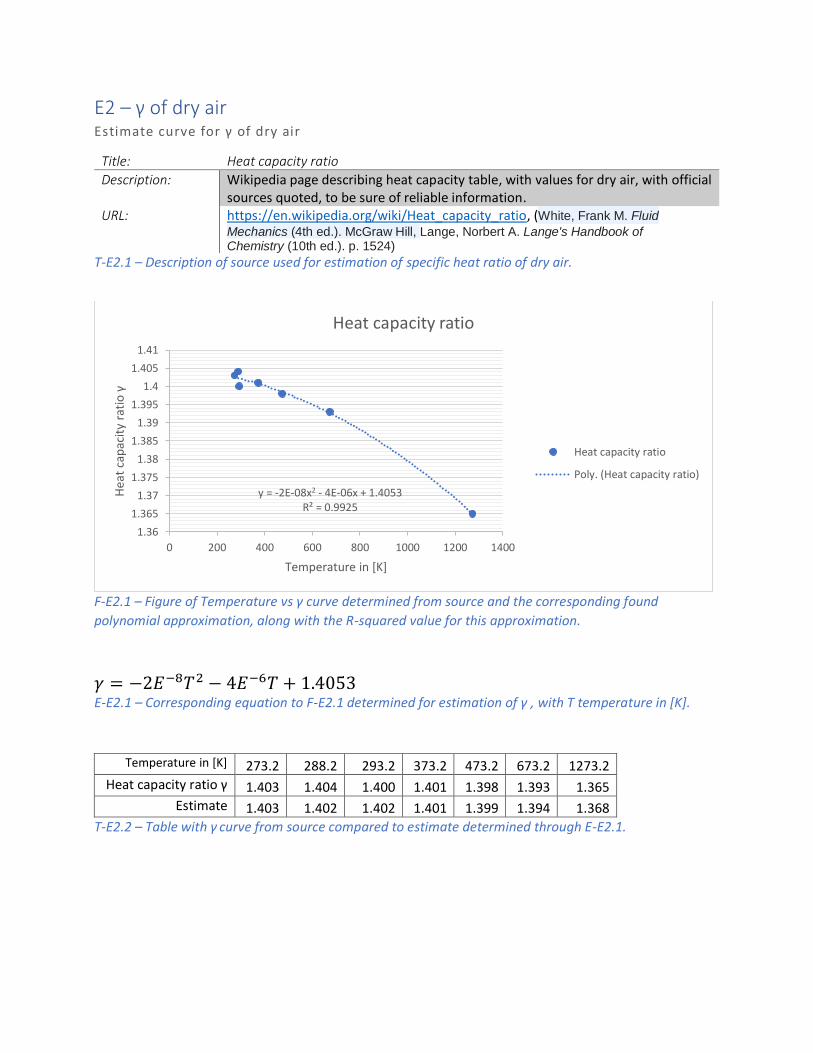
E2 – γ of dry air Estimate curve for γ of dry air

Title: Heat capacity ratio

Description: Wikipedia page describing heat capacity table, with values for dry air, with official sources quoted, to be sure of reliable information.

URL: https://en.wikipedia.org/wiki/Heat_capacity_ratio, (White, Frank M. Fluid

Mechanics (4th ed.). McGraw Hill, Lange, Norbert A. Lange's Handbook of Chemistry (10th ed.). p. 1524)

T-E2.1 – Description of source used for estimation of specific heat ratio of dry air.

F-E2.1 – Figure of Temperature vs γ curve determined from source and the corresponding found

polynomial approximation, along with the R-squared value for this approximation.

𝛾 = −2𝐸−8𝑇2 − 4𝐸−6𝑇 + 1.4053 E-E2.1 – Corresponding equation to F-E2.1 determined for estimation of γ , with T temperature in [K].

Temperature in [K] 273.2 288.2 293.2 373.2 473.2 673.2 1273.2

Heat capacity ratio γ 1.403 1.404 1.400 1.401 1.398 1.393 1.365

Estimate 1.403 1.402 1.402 1.401 1.399 1.394 1.368

T-E2.2 – Table with γ curve from source compared to estimate determined through E-E2.1.

y = -2E-08x2 - 4E-06x + 1.4053R² = 0.9925

1.36

1.365

1.37

1.375

1.38

1.385

1.39

1.395

1.4

1.405

1.41

0 200 400 600 800 1000 1200 1400

Hea

t ca

pac

ity

rati

o γ

Temperature in [K]

Heat capacity ratio

Heat capacity ratio

Poly. (Heat capacity ratio)

E3 – Resistance curve for EGT sensor Estimated resistance curve of Exhaust temperature sensor

Title: Exhaust gas temperature sensor calibration curve

Description: Official NTK manufacturer datasheet for used BM100J-CWE type sensor, from which C-type calibration curve was used.

URL: https://www.ngkntk.co.jp/resource/pdf/product_sensors_plugs_temperature_e_02.pdf T-E3.1 – Description of source used for estimation of Exhaust Temperature resistance curve.

F-E3.1 – Figure of Temperature vs resistance curve determined from source and the corresponding found

power function approximation, along with the R-squared value for this approximation.

T = 1635.5R−0.13 E-E3.1 – Corresponding equation to F-E3.1 determined for estimation of exhaust temperature T in [°C]

from measured sensor resistance R in [Ω].

Resistance in [Ω] 50000 8000 3000 500 300 100

Temperature in [°C] 400 500 600 700 800 900

Estimate 402 510 580 732 782 902

T-E3.2 – Table with temperature vs resistance curve from source compared to estimate determined

through E-E3.1.

y = 1636.5x-0.13

R² = 0.9811

0

100

200

300

400

500

600

700

800

900

1000

0 2000 4000 6000 8000 10000

Tem

per

atu

re in

[°

C]

Resistance in [Ω]

Exhaust gas temperature sensor calibration

EGT calibration

Power (EGT calibration)

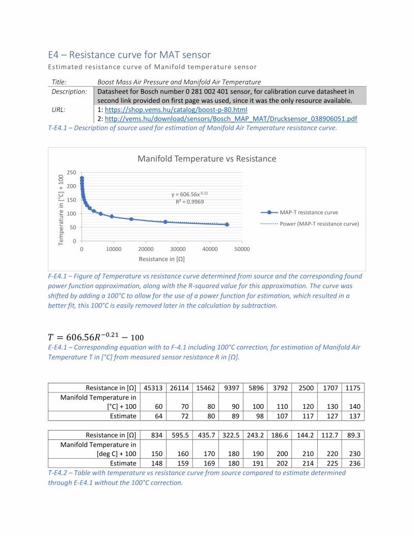
E4 – Resistance curve for MAT sensor Estimated resistance curve of Manifold temperature sensor

Title: Boost Mass Air Pressure and Manifold Air Temperature

Description: Datasheet for Bosch number 0 281 002 401 sensor, for calibration curve datasheet in second link provided on first page was used, since it was the only resource available.

URL: 1: https://shop.vems.hu/catalog/boost-p-80.html 2: http://vems.hu/download/sensors/Bosch_MAP_MAT/Drucksensor_038906051.pdf

T-E4.1 – Description of source used for estimation of Manifold Air Temperature resistance curve.

F-E4.1 – Figure of Temperature vs resistance curve determined from source and the corresponding found

power function approximation, along with the R-squared value for this approximation. The curve was

shifted by adding a 100°C to allow for the use of a power function for estimation, which resulted in a

better fit, this 100°C is easily removed later in the calculation by subtraction.

𝑇 = 606.56𝑅−0.21 − 100 E-E4.1 – Corresponding equation with to F-4.1 including 100°C correction, for estimation of Manifold Air

Temperature T in [°C] from measured sensor resistance R in [Ω].

Resistance in [Ω] 45313 26114 15462 9397 5896 3792 2500 1707 1175

Manifold Temperature in [°C] + 100 60 70 80 90 100 110 120 130 140

Estimate 64 72 80 89 98 107 117 127 137

Resistance in [Ω] 834 595.5 435.7 322.5 243.2 186.6 144.2 112.7 89.3

Manifold Temperature in [deg C] + 100 150 160 170 180 190 200 210 220 230

Estimate 148 159 169 180 191 202 214 225 236

T-E4.2 – Table with temperature vs resistance curve from source compared to estimate determined

through E-E4.1 without the 100°C correction.

y = 606.56x-0.21

R² = 0.9969

0

50

100

150

200

250

0 10000 20000 30000 40000 50000

Tem

per

atu

re in

[°C

] +

100

Resistance in [Ω]

Manifold Temperature vs Resistance

MAP-T resistance curve

Power (MAP-T resistance curve)

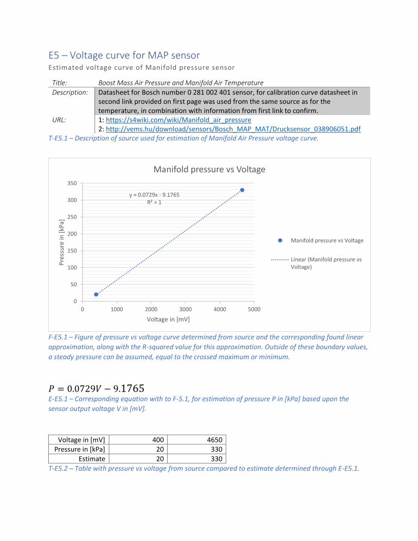
E5 – Voltage curve for MAP sensor Estimated voltage curve of Manifold pressure sensor

Title: Boost Mass Air Pressure and Manifold Air Temperature

Description: Datasheet for Bosch number 0 281 002 401 sensor, for calibration curve datasheet in second link provided on first page was used from the same source as for the temperature, in combination with information from first link to confirm.

URL: 1: https://s4wiki.com/wiki/Manifold_air_pressure 2: http://vems.hu/download/sensors/Bosch_MAP_MAT/Drucksensor_038906051.pdf

T-E5.1 – Description of source used for estimation of Manifold Air Pressure voltage curve.

F-E5.1 – Figure of pressure vs voltage curve determined from source and the corresponding found linear

approximation, along with the R-squared value for this approximation. Outside of these boundary values,

a steady pressure can be assumed, equal to the crossed maximum or minimum.

𝑃 = 0.0729𝑉 − 9.1765 E-E5.1 – Corresponding equation with to F-5.1, for estimation of pressure P in [kPa] based upon the

sensor output voltage V in [mV].

Voltage in [mV] 400 4650

Pressure in [kPa] 20 330

Estimate 20 330

T-E5.2 – Table with pressure vs voltage from source compared to estimate determined through E-E5.1.

y = 0.0729x - 9.1765R² = 1

0

50

100

150

200

250

300

350

0 1000 2000 3000 4000 5000

Pre

ssu

re in

[kP

a]

Voltage in [mV]

Manifold pressure vs Voltage

Manifold pressure vs Voltage

Linear (Manifold pressure vsVoltage)

E6 – Voltage curve of lambda sensor Estimated voltage curve Narrowband Air -Fuel ratio sensor

Title: Boost Mass Air Pressure and Manifold Air Temperature

Description: Datasheet for Bosch 0 258 005 097 Narrowband Air-Fuel ratio sensor URL: http://alflash.com.ua/for/section_A.pdf

T-E6.1 – Description of source used for estimation of Air-Fuel ratio voltage curve.

F-E6.1 – Figure of 𝜆 (lambda) value versus measured sensor voltage, with linear equations determined

from T-E6.1 and their R-squared value, for the boundary conditions the linearization’s will be extended,

with the note that the lambda value becomes less accurate the further one deviates from lambda 1.00.

𝑉𝑚𝑖𝑛 𝑖𝑛 [𝑚𝑉] 𝑉𝑚𝑎𝑥 𝑖𝑛 [𝑚𝑉] Equation of linearization

0 112 𝜆 = −0.0029𝑉 + 1.35

112 762 𝜆 = −6E−5𝑉 + 1.0269 762 1000 𝜆 = −0.0013V + 1.9779

T-E6.1 – Table of linearization’s of lambda value versus the voltage range for which they are assumed to

be valid with V measured voltage in [mV]

y = -0.0029x + 1.35R² = 1

y = -6E-05x + 1.0269R² = 1

y = -0.0013x + 1.9779R² = 1

0

0.2

0.4

0.6

0.8

1

1.2

1.4

1.6

0 200 400 600 800 1000

Lam

bd

a

Voltage in [mV]

Air-Fuel ratio linearisation curve

0 to 112 [mV]

112 to 762 [mV]

762 to 930 [mV]

Linear (0 to 112 [mV])

Linear (112 to 762 [mV])

Linear (762 to 930 [mV])

E7 – Camshaft curve Estimated camshaft profiles for measurement engine

Title: KG004 (Volvo k profile) camshaft

Description: Vendor and additional specifications on camshaft used in Volvo b230k measurement engine

URL: http://www.kgtrimning.org/tuning-special/b23b230b234/camshafts/kg004.html, https://turbobricks.com/resources.php?content=camspec

T-E7.1 – Description of source used camshaft profile estimation

F-E7.1 – Figure of actual camshaft profile markers determined from T-E7.1 versus estimate curves of

camshaft profiles.

𝐿𝑖𝑓𝑡 = 𝑝1(𝜃 − 𝐶𝑎𝑚𝑝𝑒𝑎𝑘)2 + 𝑝0 𝐶𝑎𝑚𝑝𝑒𝑎𝑘: 𝑐𝑎𝑚 𝑟𝑜𝑡𝑎𝑡𝑖𝑜𝑛 𝑓𝑜𝑟 𝑤ℎ𝑖𝑐ℎ 𝑚𝑎𝑥 𝑙𝑖𝑓𝑡 𝑜𝑐𝑐𝑢𝑟𝑠 𝑖𝑛 [𝑑𝑒𝑔] 𝐿𝑖𝑓𝑡: 𝑣𝑎𝑙𝑣𝑒 𝑙𝑖𝑓𝑡 𝑖𝑛 [𝑚] 𝑝1: 𝑠𝑒𝑐𝑜𝑛𝑑 𝑐𝑎𝑚 𝑝𝑟𝑜𝑓𝑖𝑙𝑒 𝑝𝑎𝑟𝑎𝑚𝑒𝑡𝑒𝑟, 𝑑𝑒𝑓𝑖𝑛𝑒𝑠 𝑑𝑢𝑟𝑎𝑡𝑖𝑜𝑛 𝑝0: 𝑓𝑖𝑟𝑠𝑡 𝑐𝑎𝑚 𝑝𝑟𝑜𝑓𝑖𝑙𝑒 𝑝𝑎𝑟𝑎𝑚𝑒𝑡𝑒𝑟, 𝑑𝑒𝑓𝑖𝑛𝑒𝑠 𝑝𝑒𝑎𝑘 𝑙𝑖𝑓𝑡

E-E7.1 – Corresponding equation for estimated camshaft profile curves shown in figure F-E7.1 to be used

with data from table T-E7.1.

Range 𝑝1 𝑝0 𝐶𝑎𝑚𝑝𝑒𝑎𝑘

Exhaust Valve 120 ≥ 𝜃 ≤ 378 −6.5 ∗ 10−4 11.95 249°

Intake Valve 336 ≥ 𝜃 ≤ 606 −7.1 ∗ 10−4 11.95 471°

T-E7.1 – Table of camshaft range and estimate parameters with additional information as determined

from T-E7.1.

0

2

4

6

8

10

12

14

0 100 200 300 400 500 600 700

Lift

in [

mm

]

Crankshaft rotation in degrees

Intake and exhaust estimate curves

Exhaust

Intake

Exhaust estimate

Intake Estimate

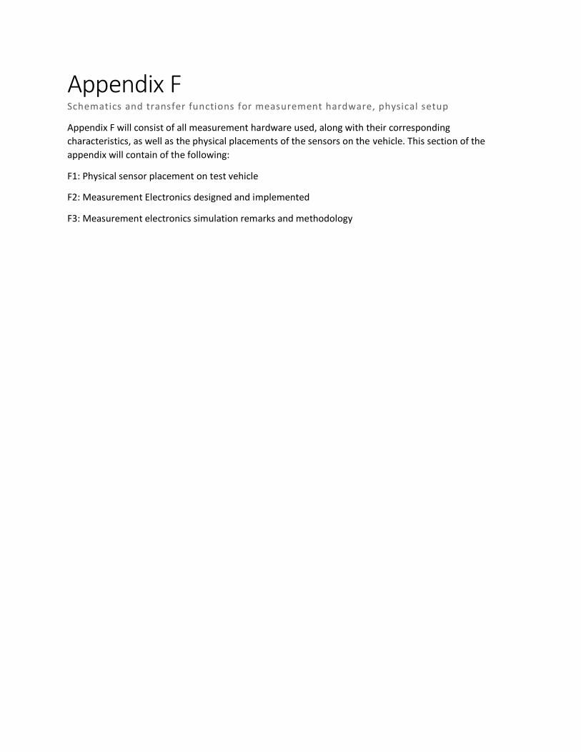
Appendix F Schematics and transfer functions for measurement hardware, physical setup

Appendix F will consist of all measurement hardware used, along with their corresponding

characteristics, as well as the physical placements of the sensors on the vehicle. This section of the

appendix will contain of the following:

F1: Physical sensor placement on test vehicle

F2: Measurement Electronics designed and implemented

F3: Measurement electronics simulation remarks and methodology

F1 – Physical sensor placement Placement of measurement devices used for comparison to model

F-F1.1 – Figure describing physical locations of all measurement sensors used on engine, for budget reasons in actual setup only one exhaust gas temperature sensor was used. [Image credit to: Bosch, NGK, Estate Services, L.M.R., Anthony Hyde]

F-F1.2a – Figure describing

Exhaust Gas Temperature

sensor in exhaust manifold,

just after the cast iron section

for the b230k engine. (circled

in red)

F-F1.2b – Figure describing

Narrowband sensor in exhaust

manifold, approximately 0.5m

from engine exhaust port of

b230k engine(circled in red)

F-F1.2c – Figure describing

Manifold Air Temperature and

Pressure sensor in Volvo b230 fuel

injection manifold (circled in red)

F2 – Measurement Electronics Measurement electronics used in datalogger device

F-F2.1 – Manifold Air Temperature sensor measurement electronics for amplifying resistance measurement into an Arduino interpretable voltage range. Wien bridge with differential amplifier reducing the measured bridge voltage by a factor of 2.2 to stay within linear range of MC3403NE operational amplifier for chosen rail voltages. The correct operation of the device was verified through LTspice.

F-F2.2 – Exhaust Gas Temperature sensor measurement electronics for amplifying resistance measurement into an Arduino interpretable voltage range. Wien bridge with differential amplifier reducing the measured bridge voltage by a factor of 2.2 to stay within linear range of MC3403NE operational amplifier for chosen rail voltages. The correct operation of the device was verified through LTspice.

𝑉𝑏𝑟𝑖𝑑𝑔𝑒 = 2.2 ∗ (𝑉𝑚𝑒𝑎𝑠 − 𝑉𝑟𝑒𝑓) [𝑉] E-F2.1 – Equation describing the measured Wien bridge voltage Vbridge in [V] based upon 𝑉meas in [V]

(output to Arduino), and power supply voltage 𝑉𝑟𝑒𝑓 𝑖𝑛 [𝑉] obtained from the power supply described in F-F2.4.

𝑅𝑚𝑒𝑎𝑠 =𝑉𝑥∗𝑅𝑏𝑟𝑖𝑑𝑔𝑒

1−𝑉𝑥[Ω] 𝑤𝑖𝑡ℎ 𝑉𝑥 =

𝑉𝑏𝑟𝑖𝑑𝑔𝑒

𝑉𝑠𝑢𝑝𝑝𝑙𝑦

E-F2.2 – Equation describing the measured sensor resistance 𝑅𝑚𝑒𝑎𝑠 𝑖𝑛 [Ω] from bridge resistors Rbridge = 1000 [Ω] (±5%), Vbridge in [V] as described in E-F2.1 and Vsupply in [V] as obtained from the

power supply described in F-F2.4.

F-F2.3 – Input protection circuitry for Manifold Air Pressure voltage measurement and Air fuel ratio measurement. Clamping diodes were used to keep Arduino analog pin between rail voltages in case of potential short circuits to battery voltage. Since both of the input voltages are not expected to get near the voltage rails in their usable range, no transfer function other than the one described in Appendix E are required. The correct operation of the device was verified through LTspice.

F-F2.4 – Power supply section for datalogger powered from noisy car battery voltage. A LM7805 voltage regulator was used to create a 5V rail to power all measurement electronics and the Arduino. With the use of a spare operational amplifier in the MC3403NE and a BC577, a stabilized center tap voltage was generated, which could be set exactly in the middle of the power supply rail with the use of the provided trim-resistor. The correct operation of the device was verified through LTspice.

F-F2.5 – Ignition event Schmitt trigger measurement device based on a MC3403NE operational amplifier with a triggering range of Vmin = 1.03 [V], Vmin = 1.47 [V] after the attenuator section of R1 and R2 to decrease the coil voltage from 0 - 14 [V] to 0 - 4.375 [V]. After the attenuator a protection circuit as described in F-F2.3 was used, with the assumption that since only a low or a high had to be detected the distortion caused by the diodes would not be a problem with the set trigger levels. The Schmitt trigger was designed with HyperPhysics and the correct operation of the device was verified through LTspice.

F-F2.6 – Physical construction of datalogger device, on bottom left of the left picture the operational

amplifier section can be seen, the top left of the left picture shows the Arduino with an expansion

shield for extra board space. For the connections Neutrix connectors were used for a robust

connection, along with an aluminum enclosure which was be mounted to the vehicle and plugged in to

the sensor wiring loom, as shown in the right picture

F3: Measurement electronics simulation Remarks and details of methodology

Resistance measurement:

F-F3.1a,b – LTspice schematics used for verification of resistance measurement circuitry. Since a

MC3403NE simulation model was not available, the already included simulation of the OP495 as

described by Digchip. The power supply was also included to simulate sag in the supply lines. Assuming

a resistance range from 50𝑘Ω to 50Ω a current sweep for the EGT sensor was determined of roughly

100μA to 5mA in the schematic configuration if no current draw into the amplifier is assumed. Since

both the EGT and MAT sensor feature the same resistance range and measurement schematic, the

results are valid for both and are shown in F-F3.2 and F-F3.3 below.

F-F3.2 – Simulation result for F-F3.1 for Wien bridge voltage compared to the current sweep, showing

that the bridge was approximately configured for a zero swing at 2.5 mA or 1000Ω roughly centered in

the measurement range. More swing towards the lower resistances is chosen with this value, since it can

be seen in F-E3.1 and F-E4.1 that those measurement are in the range of expected measurement signals

from the model.

F-F3.3 – Simulation result of measurement bridge voltage compared 𝑉𝑚𝑒𝑎𝑠/𝑉𝑎𝑟𝑑𝑢𝑖𝑛𝑜_𝑎1, as can be

seen, 𝑉𝑚𝑒𝑎𝑠 is according to E-F2.1, with Vmeas = 3.6 [V] for Vbridge = 2.4 [V] and 𝑉𝑚𝑒𝑎𝑠 =

1.4[V] 𝑓𝑜𝑟 𝑉bridge = −2.4 [𝑉], maintaining the from E-F2.1 expected relationship.

Voltage measurement:

F-F3.4 – LTspice schematics used for verification of voltage measurement circuitry. As seen above the

power supply was modelled as a source with Rserial = 5 as assumption of the output impedance of the

LM7805 voltage regulator. A sweep of 0 − 5 [V] was chosen for the MAP sensor according to T-E5.1, and

a sweep of 0 − 1 [V] was chosen for the Narrowband sensor according to T-E6.1.

F-F3.5 – Simulation result for 𝑉arduino_a2 which can be assumed equal to that of 𝑉arduino_a3 since for both

the component selection is the same and for 𝑉arduino_a3 the voltage swing is shorter. As observed the

voltage closely follows the sweep with only a slight deviation at Vpmap = 0.75 [V], which after a closer

look turned out to be a difference of 0.04 [mV], which is insignificant to comparison to the sensor

accuracy as shown in T-E5.1, T-E6.1.

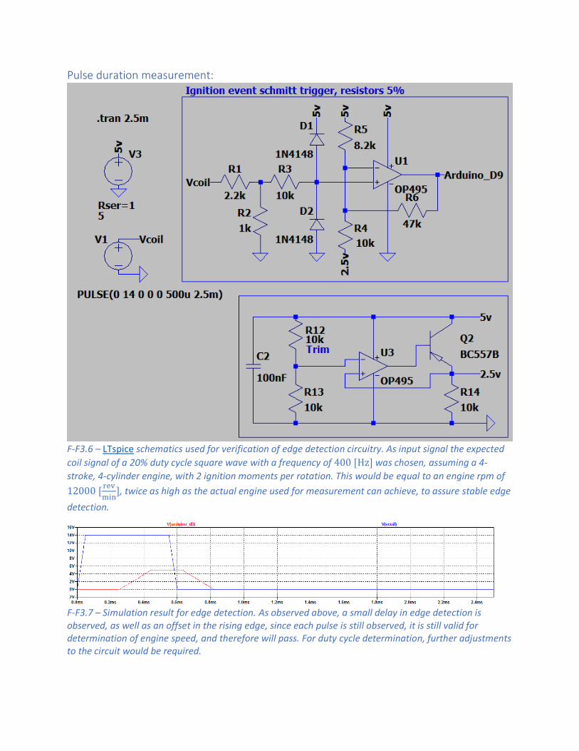
Pulse duration measurement:

F-F3.6 – LTspice schematics used for verification of edge detection circuitry. As input signal the expected

coil signal of a 20% duty cycle square wave with a frequency of 400 [Hz] was chosen, assuming a 4-

stroke, 4-cylinder engine, with 2 ignition moments per rotation. This would be equal to an engine rpm of

12000 [rev

min], twice as high as the actual engine used for measurement can achieve, to assure stable edge

detection.

F-F3.7 – Simulation result for edge detection. As observed above, a small delay in edge detection is observed, as well as an offset in the rising edge, since each pulse is still observed, it is still valid for determination of engine speed, and therefore will pass. For duty cycle determination, further adjustments to the circuit would be required.

Power Supply:

F-F3.8 – LTspice schematics used for verification of power supply circuitry. The voltage regulator is

assumed to have a 𝑅series = 5 [Ω] , The current draw from the 5 [V] and 2.5 [V] lines are estimated to

have a current draw of 50mA.

F-F3.9 – Simulation result for Vsupply with a current draw of 50 [mA], a voltage drop of 0.107 [V] can be

observed, which is deemed acceptable.

F-F3.10 Simulation result for Vref with a current draw of 50 [mA], as shown in F-F3.9, the value observed above is exact half of Vsupply which can be deemed as correct.

Appendix G Code sections for model and measurement

Appendix G will consist of all code used for the measurement and modelling of the combustion engine.

This section of the appendix will contain of the following:

G1: Arduino code for datalogger

G2: MATLAB code for file scraper/plotter

G3: Main MATLAB code for combustion engine model

G4: Subfunctions for main MATLAB model

G5: Combustion engine overview.

G1 – Arduino code for datalogger Final version of code used

// Define variables for prescale of ADC for faster analogread

#define cbi(sfr, bit) (_SFR_BYTE(sfr) &= ~_BV(bit))

#define sbi(sfr, bit) (_SFR_BYTE(sfr) |= _BV(bit))

// Configure for sensors

const int TMAP = A0; // Manifold temperature analog pin on arduino

const int EGT = A1; // Exhaust temperature analog pin on arduino

const int MAP = A2; // Manifold pressure analog pin on arduino

const int Lambda = A3; // Air fuel mixture analog pin on arduino

int Vtmap = 0; // Constant for storing measured analog value of Manifold

temperature

int Vegt = 0; // Constant for storing measured analog value of Exhaust

temperature

int Vmap = 0; // Constant for storing measured analog value of Manifold

pressure

int Vlambda = 0; // Constant for storing measured analog value of Air fuel

mixture

int Wheel = 9; // Define pin 9 as the Wheel speed measurement

int Engine = 8; // Define pin 8 as the Engine speed measurement

int Wheelpulse = 0; // int for storing high or low of wheel pulse

int Enginepulse =0; // int for storing high or low of wheel pulse

int t0 = 0;

int t = 0;

String dataString = "";

void setup() {

// Change prescale of ADC clock for faster analogread

sbi(ADCSRA, ADPS2);

cbi(ADCSRA, ADPS1);

cbi(ADCSRA, ADPS0);

// initialize status led pin

pinMode(7,OUTPUT);

// initialize Wheel speed and Engine speed pins

pinMode(Wheel,INPUT);

pinMode(Engine,INPUT);

// Initialize serial communication for RTC and sd

Serial.begin(115200);

// then writing status led on for active in code

digitalWrite(7, HIGH);

}

void loop() {

Serial.println(ReadSignals());

}

String ReadSignals(){

// start timing measurement duration

t0 = micros();

// make a string for assembling the data to log:

dataString = "";

// Read and print Manifold temperature measurement

Vtmap = analogRead(TMAP);

dataString += String(Vtmap);

dataString += ",";

// Read and print Exhaust temperature measurement

Vegt = analogRead(EGT);

dataString += String(Vegt);

dataString += ",";

// Read and print Manifold pressure measurement

Vmap = analogRead(MAP);

dataString += String(Vmap);

dataString += ",";

// Read and print Air fuel mixture measurement

Vlambda = analogRead(Lambda);

dataString += String(Vlambda);

dataString += ",";

// Read and print Wheel speed

Wheelpulse = digitalRead(Wheel);

dataString += String(Wheelpulse);

dataString += ",";

// Read and print Engine speed

Enginepulse = digitalRead(Engine);

dataString += String(Enginepulse);

dataString += ",";

t = micros() - t0;

dataString += String(t);

return dataString;

}

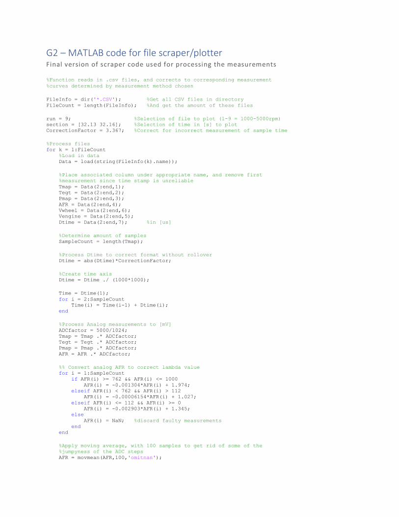
G2 – MATLAB code for file scraper/plotter Final version of scraper code used for processing the measurements

%Function reads in .csv files, and corrects to corresponding measurement %curves determined by measurement method chosen

FileInfo = dir('*.CSV'); %Get all CSV files in directory FileCount = length(FileInfo); %And get the amount of these files

run = 9; %Selection of file to plot (1-9 = 1000-5000rpm) section = [32.13 32.16]; %Selection of time in [s] to plot CorrectionFactor = 3.367; %Correct for incorrect measurement of sample time

%Process files for k = 1:FileCount %Load in data Data = load(string(FileInfo(k).name));

%Place associated column under appropriate name, and remove first %measurement since time stamp is unreliable Tmap = Data(2:end,1); Tegt = Data(2:end,2); Pmap = Data(2:end,3); AFR = Data(2:end,4); Vwheel = Data(2:end,6); Vengine = Data(2:end,5); Dtime = Data(2:end,7); %in [us]

%Determine amount of samples SampleCount = length(Tmap);

%Process Dtime to correct format without rollover Dtime = abs(Dtime)*CorrectionFactor;

%Create time axis Dtime = Dtime ./ (1000*1000);

Time = Dtime(1); for i = 2:SampleCount Time(i) = Time(i-1) + Dtime(i); end

%Process Analog measurements to [mV] ADCfactor = 5000/1024; Tmap = Tmap .* ADCfactor; Tegt = Tegt .* ADCfactor; Pmap = Pmap .* ADCfactor; AFR = AFR .* ADCfactor;

%% Convert analog AFR to correct lambda value for i = 1:SampleCount if AFR(i) >= 762 && AFR(i) <= 1000 AFR(i) = -0.001304*AFR(i) + 1.974; elseif AFR(i) < 762 && AFR(i) > 112 AFR(i) = -0.00006154*AFR(i) + 1.027; elseif AFR(i) <= 112 && AFR(i) >= 0 AFR(i) = -0.002903*AFR(i) + 1.345; else AFR(i) = NaN; %discard faulty measurements end end

%Apply moving average, with 100 samples to get rid of some of the %jumpyness of the ADC steps AFR = movmean(AFR,100,'omitnan');

%% Convert MAP pressure to correct value in [kPa] for i = 1:SampleCount if Pmap(i) >= 400 && Pmap(i) <= 4650 Pmap(i) = 0.07294*Pmap(i) - 9.176; else Pmap(i) = Pmap(i-1); %discard faulty measurements end end

%% Convert MAP temperature to correct value in [C°] Rbrid = 1000; %Bridge resitors Vref = 2.5; %Reference voltage [V] Vsup = 5.0; %Bridge supply voltage [V] for i = 1:SampleCount Vmeas = Tmap(i)/1000; %Convert and get Vmeas [V] Vx = (2*Vmeas - Vref)/Vsup; %Get intermediate voltage Vx Rmeas = (Rbrid*Vx)/(1-Vx); %Get measured resistance Tmap(i) = -100 + 606.5*Rmeas^-0.21; %Get actual temperature from calibration curve end

%Apply moving average, with 100 samples to get rid of some of the %jumpyness of the ADC steps Tmap = movmean(Tmap,100,'omitnan');

%% Convert EGT temperature to correct value in [C°] Rbrid = 1000; %Bridge resitors Vref = 2.5; %Reference voltage [V] Vsup = 5.0; %Bridge supply voltage [V] for i = 1:SampleCount Vmeas = Tegt(i)/1000; %Convert and get Vmeas [V] Vx = (2*Vmeas - Vref)/Vsup; %Get intermediate voltage Vx Rmeas = (Rbrid*Vx)/(1-Vx); %Get measured resistance Tegt(i) = 1641.6*Rmeas^-0.13; %Get actual temperature from calibration curve end

%Apply moving average, with 100 samples to get rid of some of the %jumpyness of the ADC steps Tegt = movmean(Tegt,100,'omitnan');

%% Convert Vengine to rpm signal PrevIndice = 1; %Make variable for start of period indices Vengine(1) = 0; %Start engine speed signal at 0 to prevent errors TimeOut = 0.5; %Define max value for no pulse to keep signal reasonoable PulsePerRot = 2; %Define spark events per rotation RotationIndice = []; %Create variable to store engine rotation indices in

for i = 2:SampleCount-1 if Vengine(i) == 0 && Vengine(i+1) == 1 Vengine(i) = Time(i) - Time(PrevIndice); PrevIndice = i; RotationIndice = [RotationIndice PrevIndice]; if Vengine(i) > TimeOut Vengine(i) = 0; %Assume engine not running end else Vengine(i) = Vengine(i-1); end end Vengine(SampleCount) = Vengine(i-1);

%Determine measured ignition pulse frequency Vengine = 1 ./ Vengine;

%Correct for cylinder count of engine Vengine = Vengine ./ PulsePerRot;

%Apply moving average, with 100 samples to get rid of some of the jumpyness of the ADC steps Vengine = movmean(Vengine,100,'omitnan');

%Convert to rev/min Vengine = Vengine * 60;

%% Convert Vwheel to Wheelpulse signal PrevIndice = 1; %Make variable for start of period indices Vwheel(1) = 0; %Start engine speed signal at 0 to prevent errors TimeOut = 0.5; %Define max value for no pulse to keep signal reasonoable PulsePerRot = 48; %Define how many spark events per rotation

for i = 2:SampleCount-1 if Vwheel(i) == 0 && Vwheel(i+1) == 1 Vwheel(i) = Time(i) - Time(PrevIndice); PrevIndice = i; if Vwheel(i) > TimeOut Vwheel(i) = 0; %Assume engine not running end else Vwheel(i) = Vwheel(i-1); end end Vwheel(SampleCount) = Vwheel(i-1);

%Convert to frequency measured for pulse Vwheel = PulsePerRot ./ Vwheel;

%Convert to actual speed in km/h %Wheel size r15 205/60 Circumference = 1.965; %circumference in m Vwheel = Circumference * Vwheel; %Convert speed to m/s Vwheel = 3.6 * Vwheel; %Convert to km/h

%% Plot results if run == k %Deterimine section indices a = find(Time > section(1)); b = find(Time > section(2)); if isempty(b) b = SampleCount; end

% Plot Manifold Temperature clear 1 figure(1)

subplot(3,2,1); hold on plot(Time(a(1):b(1)),Tmap(a(1):b(1)),'Color','b') Average = mean(Tmap(a(1):b(1))); plot(Time([a(1) b(1)]),[Average Average],'Color','r') text(Time(b(1)),Average,string(Average)); title('Manifold temperature') xlabel('Time in [s]') ylabel('Temperature in [C°]') hold off

% Plot Manifold Pressure subplot(3,2,2); hold on plot(Time(a(1):b(1)),Pmap(a(1):b(1)),'Color','b') Average = mean(Pmap(a(1):b(1))); plot(Time([a(1) b(1)]),[Average Average],'Color','r') text(Time(b(1)),Average,string(Average)); title('Manifold pressure') xlabel('Time in [s]') ylabel('Pressure in [kPa]') hold off

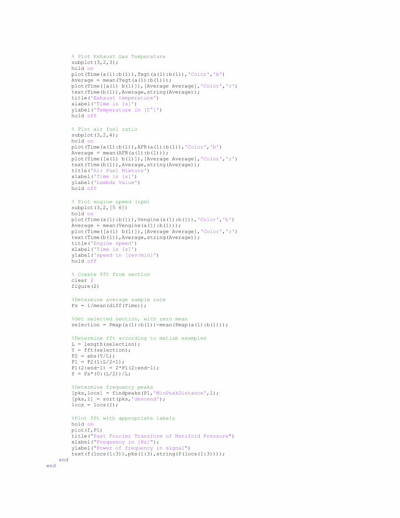
% Plot Exhaust Gas Temperature subplot(3,2,3); hold on plot(Time(a(1):b(1)),Tegt(a(1):b(1)),'Color','b') Average = mean(Tegt(a(1):b(1))); plot(Time([a(1) b(1)]),[Average Average],'Color','r') text(Time(b(1)),Average,string(Average)); title('Exhaust temperature') xlabel('Time in [s]') ylabel('Temperature in [C°]') hold off

% Plot air fuel ratio subplot(3,2,4); hold on plot(Time(a(1):b(1)),AFR(a(1):b(1)),'Color','b') Average = mean(AFR(a(1):b(1))); plot(Time([a(1) b(1)]),[Average Average],'Color','r') text(Time(b(1)),Average,string(Average)); title('Air Fuel Mixture') xlabel('Time in [s]') ylabel('Lambda Value') hold off

% Plot engine speed (rpm) subplot(3,2,[5 6]) hold on plot(Time(a(1):b(1)),Vengine(a(1):b(1)),'Color','b') Average = mean(Vengine(a(1):b(1))); plot(Time([a(1) b(1)]),[Average Average],'Color','r') text(Time(b(1)),Average,string(Average)); title('Engine speed') xlabel('Time in [s]') ylabel('speed in [rev/min]') hold off

% Create fft from section clear 2 figure(2)

%Determine average sample rate Fs = 1/mean(diff(Time));

%Get selected section, with zero mean selection = Pmap(a(1):b(1))-mean(Pmap(a(1):b(1)));

%Determine fft according to matlab examples L = length(selection); Y = fft(selection); P2 = abs(Y/L); P1 = P2(1:L/2+1); P1(2:end-1) = 2*P1(2:end-1); f = Fs*(0:(L/2))/L;

%Determine frequency peaks [pks,locs] = findpeaks(P1,'MinPeakDistance',1); [pks,I] = sort(pks,'descend'); locs = locs(I);

%Plot fft with appropriate labels hold on plot(f,P1) title("Fast Fourier Transform of Manifold Pressure") xlabel("Frequency in [Hz]"); ylabel("Power of frequency in signal") text(f(locs(1:3)),pks(1:3),string(f(locs(1:3)))); end end

G3 – Main MATLAB code for combustion engine model Final version combustion engine model used for comparison to measurements

%Make sure to start with a clean run

clear all

%Indicate determined AFR

LambdaRead = 1;

%Rpm specification

PistonSpec.Rpm = 2000;

%% Guess as to throttle plate opening

rtb = 25/1000; %Throttle body radius estimate

Cdtb = 0.86; %Estimate of throttle body flow efficiency [ratio]

opening = 1; %Estimate of throttle body opening in %

%Calculate effective area

Atb = pi*rtb*rtb*(opening/100); %Calculate flow area

Aefftb = Atb * Cdtb; %Calculate effective flow area

%% Create Piston Specification

% Piston specifications (b230)

PistonSpec.Bore = 96/1000; %Bore in (m)

PistonSpec.Stroke = 80/1000; %Stroke in (m)

PistonSpec.Compression = 10.3; %Compression ratio

PistonSpec.Lconnect = 152/1000; %Length of connecting rod in (m)

PistonSpec.FullRotation = 720; %Specify rotation required for full rotation (2/4 stroke)

% Define specific heat constant for dry air

Rair = 287.058;

% Calculate cylinder and chamber specifications

PistonSpec.Apiston = pi*(PistonSpec.Bore/2)*(PistonSpec.Bore/2); %Determine piston area

(m^2)

PistonSpec.Vstroke = PistonSpec.Stroke*PistonSpec.Apiston; %Determine volume in

stroked area (m^3)

PistonSpec.Vchamber = PistonSpec.Vstroke/(PistonSpec.Compression - 1); %Determine volume in

combustion chamber(m^3)

%% Initialize outside air variables

Athmos.P = 101.325*1000; %Outside air pressure in [Pa]

Athmos.T = 20 + 273.15; %Outside air temperature in [deg K]

%Calculate outside air density

Athmos.Rho = Athmos.P/(Rair*Athmos.T);

%% Initialize plenum variables

Plenum.P = Athmos.P; % Estimate at start Plenum is at Pathmos

Plenum.V = 2.376/1000; % Estimate of plenum size with runners in [L]

Plenum.T = Athmos.T;

%Calculate starting air mass in plenum

Plenum.M = (Plenum.P*Plenum.V)/(Rair*Plenum.T);

%Calculate starting air densisty in plenum

Plenum.Rho = Plenum.M/Plenum.V;

%Calculate starting energy in plenum

Cv = getCv(Plenum.T);

Plenum.Q = Plenum.M*Cv*Plenum.T;

%% Initialize PistonCalc with plenum = chamber at bdc assumption for intake stroke

%Assume plenum temperature is chamber temperature at bdc

PistonInit.T = Plenum.T;

%Chamber volume with full stroke at 180 deg of rotation

PistonInit.V = PistonSpec.Vstroke + PistonSpec.Vchamber;

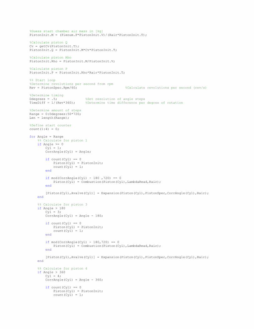
%Guess start chamber air mass in [kg]

PistonInit.M = (Plenum.P*PistonInit.V)/(Rair*PistonInit.T);

%Calculate piston Q

Cv = getCv(PistonInit.T);

PistonInit.Q = PistonInit.M*Cv*PistonInit.T;

%Calculate piston Rho

PistonInit.Rho = PistonInit.M/PistonInit.V;

%Calculate piston P

PistonInit.P = PistonInit.Rho*Rair*PistonInit.T;

%% Start loop

%Determine revolutions per second from rpm

Rev = PistonSpec.Rpm/60; %Calculate revolutions per second (rev/s)

%Determine timing

Ddegrees = .5; %Set resolution of angle steps

TimeDiff = 1/(Rev*360); %Determine time difference per degree of rotation

%Determine amount of steps

Range = 0:Ddegrees:50*720;

Len = length(Range);

%Define start counter

count(1:4) = 0;

for Angle = Range

%% Calculate for piston 1

if Angle >= 0

Cyl = 1;

CorrAngle(Cyl) = Angle;

if count(Cyl) == 0

Piston(Cyl) = PistonInit;

count(Cyl) = 1;

end

if mod(CorrAngle(Cyl) - 180 ,720) == 0

Piston(Cyl) = Combustion(Piston(Cyl),LambdaRead,Rair);

end

[Piston(Cyl),Avalve(Cyl)] = Expansion(Piston(Cyl),PistonSpec,CorrAngle(Cyl),Rair);

end

%% Calculate for piston 3

if Angle > 180

Cyl = 3;

CorrAngle(Cyl) = Angle - 180;

if count(Cyl) == 0

Piston(Cyl) = PistonInit;

count(Cyl) = 1;

end

if mod(CorrAngle(Cyl) - 180,720) == 0

Piston(Cyl) = Combustion(Piston(Cyl),LambdaRead,Rair);

end

[Piston(Cyl),Avalve(Cyl)] = Expansion(Piston(Cyl),PistonSpec,CorrAngle(Cyl),Rair);

end

%% Calculate for piston 4

if Angle > 360

Cyl = 4;

CorrAngle(Cyl) = Angle - 360;

if count(Cyl) == 0

Piston(Cyl) = PistonInit;

count(Cyl) = 1;

end

if mod(CorrAngle(Cyl) - 180,720) == 0

Piston(Cyl) = Combustion(Piston(Cyl),LambdaRead,Rair);

end

[Piston(Cyl),Avalve(Cyl)] = Expansion(Piston(Cyl),PistonSpec,CorrAngle(Cyl),Rair);

end

%% Calculate for piston 2

if Angle > 540

Cyl = 2;

CorrAngle(Cyl) = Angle - 540;

if count(Cyl) == 0

Piston(Cyl) = PistonInit;

count(Cyl) = 1;

end

if mod(CorrAngle(Cyl) - 180,720) == 0

Piston(Cyl) = Combustion(Piston(Cyl),LambdaRead,Rair);

end

[Piston(Cyl),Avalve(Cyl)] = Expansion(Piston(Cyl),PistonSpec,CorrAngle(Cyl),Rair);

end

%%Determine flows

TimeStep = TimeDiff * Ddegrees; %Determine delta in seconds per loop iteration

[Piston,Plenum,Flows] = Flow(Piston,Avalve,Plenum,Athmos,TimeStep,Rair,Aefftb); %Call flows

function for calculation

%% Determine results

Result(1+(Angle/Ddegrees)).Tplenum = Plenum.T;

Result(1+(Angle/Ddegrees)).Pplenum = Plenum.P;

Result(1+(Angle/Ddegrees)).Tpiston = Piston(1).T;

Result(1+(Angle/Ddegrees)).Ppiston = Piston(1).P;

Result(1+(Angle/Ddegrees)).Vpiston = Piston(1).V;

Result(1+(Angle/Ddegrees)).Mpiston = Piston(1).M;

Result(1+(Angle/Ddegrees)).AeffIn = Avalve(1).Ain;

Result(1+(Angle/Ddegrees)).AeffOut = Avalve(1).Aex;

Result(1+(Angle/Ddegrees)).FlowIn = Flows(1).In;

Result(1+(Angle/Ddegrees)).FlowOut = Flows(1).Ex;

end

%% Plot 'short' run

%Section specification

Section = [720*49 720*50] - 540;

clear 1

figure(1)

%Determine plot section

Angles = Section(1):Ddegrees:Section(2);

Time = Angles*TimeDiff;

Indices = Angles./Ddegrees;

%Plot the valve area calculated

subplot(4,2,4);

hold on

In = [Result(Indices+1).AeffIn];

Out = [Result(Indices+1).AeffOut];

plot(Time,In,'b')

plot(Time,Out,'r')

title('Valve opening piston 1 (red = exhaust, blue = intake)')

xlabel('Time in [s]')

ylabel('Effective area in [m^2]')

%Determine peak and start of curve for cams

[~,indiceIn] = max(In);

for k = 1:length(In)-1

if In(k) == 0 && In(k+1) > 0

indiceIn = [indiceIn k];

end

if In(k+1) == 0 && In(k) > 0

indiceIn = [indiceIn k+1];

end

end

scatter(Time(indiceIn),In(indiceIn),'b*')

[~,indiceEx] = max(Out);

for k = 1:length(Out)-1

if Out(k) == 0 && Out(k+1) > 0

indiceEx = [indiceEx k];

end

if Out(k+1) == 0 && Out(k) > 0

indiceEx = [indiceEx k+1];

end

end

scatter(Time(indiceEx),Out(indiceEx),'r*')

hold off

%Plot the Plenum Temperature

subplot(4,2,1);

hold on

Tplenum = [Result(Indices+1).Tplenum]-273.15;

plot(Time,Tplenum)

plot([Time(1) Time(end)],[mean(Tplenum) mean(Tplenum)],'r')

text(Time(end),mean(Tplenum),string(mean(Tplenum)));

title('Manifold temperature')

xlabel('Time in [s]')

ylabel('Temperature in [C°]')

hold off

%Plot Manifold Pressure

subplot(4,2,2);

hold on

Pplenum = [Result(Indices+1).Pplenum]./1000;

plot(Time,Pplenum)

plot([Time(1) Time(end)],[mean(Pplenum) mean(Pplenum)],'r')

text(Time(end),mean(Pplenum),string(mean(Pplenum)));

title('Manifold pressure')

xlabel('Time in [s]')

ylabel('Pressure in [kPa]')

%Add markers of valve timing

scatter(Time(indiceIn),Pplenum(indiceIn),'b*')

scatter(Time(indiceEx),Pplenum(indiceEx),'r*')

hold off

%Plot Piston Mass

subplot(4,2,8);

hold on

Mpiston = [Result(Indices+1).Mpiston]./1000;

plot(Time,Mpiston)

title('Air Mass in piston')

xlabel('Time in [s]')

ylabel('Mass in [kg]')

%Add markers of valve timing

scatter(Time(indiceIn),Mpiston(indiceIn),'b*')

scatter(Time(indiceEx),Mpiston(indiceEx),'r*')

hold off

%Plot chamber Volume

subplot(4,2,7);

hold on

Vpiston = [Result(Indices+1).Vpiston].*10^6;

plot(Time, Vpiston)

title('Piston volume of cylinder 1')

xlabel('Time in [s]')

ylabel('Volume in [cm^3]')

%Add markers of valve timing

scatter(Time(indiceIn),Vpiston(indiceIn),'b*')

scatter(Time(indiceEx),Vpiston(indiceEx),'r*')

hold off

%Plot chamber Pressure

subplot(4,2,3)

hold on

Ppiston = [Result(Indices+1).Ppiston]./1000;

plot(Time,Ppiston)

title('Piston pressure of cylinder 1')

xlabel('Time in [s]')

ylabel('Pressure in [kPa]')

%Add markers of valve timing

scatter(Time(indiceIn),Ppiston(indiceIn),'b*')

scatter(Time(indiceEx),Ppiston(indiceEx),'r*')

hold off

%Plot Piston Temperature

subplot(4,2,5)

hold on

Tpiston = [Result(Indices+1).Tpiston]-273.15;

plot(Time, Tpiston)

title('Piston temperature of cylinder 1')

xlabel('Time in [s]')

ylabel('Temperature in [deg C]')

%Add markers of valve timing

scatter(Time(indiceIn),Tpiston(indiceIn),'b*')

scatter(Time(indiceEx),Tpiston(indiceEx),'r*')

hold off

hold off

%Plot intake and exhaust flow in kg/s

subplot(4,2,6);

hold on

In = [Result(Indices+1).FlowIn];

Out = [Result(Indices+1).FlowOut];

plot(Time,In,'b')

plot(Time,Out,'r')

title('Mass flow of valves (red = exhaust, blue = intake)')

xlabel('Time in [s]')

ylabel('Flow in [kg]')

%% Plot P-V diagram

clear 5

figure(5)

plot(Vpiston,Ppiston)

title('P-V Diagram for engine')

xlabel('Voume in [cm^3]')

ylabel('Pressure in [Pa]')

%% Plot 'long' run

%Section specification

Section = [40*720 50*720];

clear 2

figure(2)

%Determine time

Angles = Section(1):Ddegrees:Section(2);

Time = Angles*TimeDiff;

Indices = Angles./Ddegrees;

%Plot Manifold Temperature

subplot(3,2,1);

hold on

Tplenum = [Result(Indices+1).Tplenum]-273.15;

plot(Time,Tplenum)

plot([Time(1) Time(end)],[mean(Tplenum) mean(Tplenum)],'r')

text(Time(end),mean(Tplenum),string(mean(Tplenum)));

title('Manifold temperature')

xlabel('Time in [s]')

ylabel('Temperature in [C°]')

hold off

%Plot Manifold Pressure

subplot(3,2,2);

hold on

Pplenum = [Result(Indices+1).Pplenum]./1000;

plot(Time,Pplenum)

plot([Time(1) Time(end)],[mean(Pplenum) mean(Pplenum)],'r')

text(Time(end),mean(Pplenum),string(mean(Pplenum)));

title('Manifold pressure')

xlabel('Time in [s]')

ylabel('Pressure in [kPa]')

%Plot Piston Pressure

subplot(3,2,3)

hold on

plot(Time,[Result(Indices+1).Ppiston]./1000)

title('Piston pressure of cylinder 1')

xlabel('Time in [s]')

ylabel('Pressure in [kPa]')

hold off

%Plot effective area of intake and exhaust valve

subplot(3,2,4);

hold on

plot(Time,[Result(Indices+1).AeffIn],'b')

plot(Time,[Result(Indices+1).AeffOut],'r')

title('Valve opening piston 1 (red = exhaust, blue = intake)')

xlabel('Time in [s]')

ylabel('Effective area in [m^2]')

hold off

%Plot Chamber Temperature

subplot(3,2,5)

hold on

Tpiston = [Result(Indices+1).Tpiston] -273.15;

plot(Time, Tpiston)

plot([Time(1) Time(end)],[mean(Tpiston) mean(Tpiston)],'r')

text(Time(end),mean(Tpiston),string(mean(Tpiston)));

title('Piston temperature of cylinder 1')

xlabel('Time in [s]')

ylabel('Temperature in [deg C]')

hold off

%Plot chamber Volume

subplot(3,2,6);

Vpiston = [Result(Indices+1).Vpiston].*10^6;

plot(Time, Vpiston)

title('Piston volume of cylinder 1')

xlabel('Time in [s]')

ylabel('Volume in [cm^3]')

%Plot frequency spectrum

figure(3)

%Determine average sample rate

Fs = 1/mean(diff(Time));

%Get selected section, with zero mean

selection = Pplenum-mean(Pplenum);

%Determine fft according to matlab examples

L = length(selection);

Y = fft(selection);

P2 = abs(Y/L);

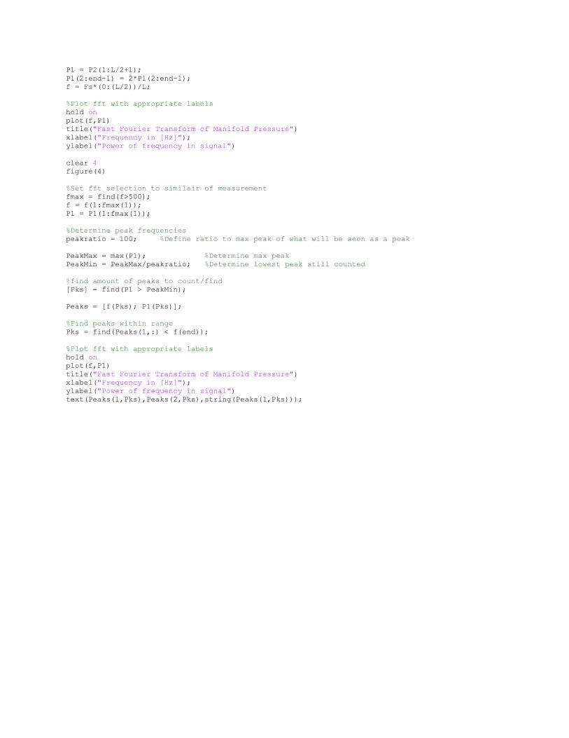
P1 = P2(1:L/2+1);

P1(2:end-1) = 2*P1(2:end-1);

f = Fs*(0:(L/2))/L;

%Plot fft with appropriate labels

hold on

plot(f,P1)

title("Fast Fourier Transform of Manifold Pressure")

xlabel("Frequency in [Hz]");

ylabel("Power of frequency in signal")

clear 4

figure(4)

%Set fft selection to similair of measurement

fmax = find(f>500);

f = f(1:fmax(1));

P1 = P1(1:fmax(1));

%Determine peak frequencies

peakratio = 100; %Define ratio to max peak of what will be seen as a peak

PeakMax = max(P1); %Determine max peak

PeakMin = PeakMax/peakratio; %Determine lowest peak still counted

%find amount of peaks to count/find

[Pks] = find(P1 > PeakMin);

Peaks = [f(Pks); P1(Pks)];

%Find peaks within range

Pks = find(Peaks(1,:) < f(end));

%Plot fft with appropriate labels

hold on

plot(f,P1)

title("Fast Fourier Transform of Manifold Pressure")

xlabel("Frequency in [Hz]");

ylabel("Power of frequency in signal")

text(Peaks(1,Pks),Peaks(2,Pks),string(Peaks(1,Pks)));

G4 – Subfunctions for main MATLAB model Final versions of subfunctions used in combustion engine model

GetCv: function Cv = getCv(Temp)

%% Determine Delta temperature assuming constant volume

r0 = 0.6512; % constant term for approximation of Cv

r1 = 0.0002; % linear term for approximation of Cv

r2 = 0.000000009; % kwadratic term for approximation of Cv

Cv = r2*Temp*Temp + r1*Temp + r0; %Determine Cv of dry air for starting temperature in [kJ*kg-

1*K-1]

Expansion: function [Piston,Avalve] = Expansion(Piston,PistonSpec,Angle,Rair)

%% Convert angle

Angle = mod(Angle, PistonSpec.FullRotation);

%% Calculate piston speed

%Determine correct piston model angle

Angle2 = (4*pi*Angle)/PistonSpec.FullRotation;

%Determine y postion of piston relative to angle (m)

y = (PistonSpec.Stroke/2)*cos(Angle2) + sqrt(PistonSpec.Lconnect^2 -

((PistonSpec.Stroke/2)*sin(Angle2))^2);

%Determine y position based on stroke

y = y - PistonSpec.Lconnect + PistonSpec.Stroke/2; %Correct to piston bottom = 0

%% Determine valve lifts

In1 = -0.00065; %Intake x^2 term

In0 = 11.95; %Intake constant term

Ex1 = -0.00071; %Exhaust x^2 term

Ex0 = 11.95; %Exhaust constant term

if Angle >= 120 && Angle <= 606

if Angle >= 120 && Angle <= 378

Ang = Angle - 249; %Correct to use x^2 equation

LiftEx = Ex1*Ang*Ang + Ex0; %Calculate exhaust lift

else

LiftEx = 0; %In case no lift set lift 0

end

if Angle >= 336 && Angle <= 606

Ang = Angle - 471; %Correct to use x^2 equation

LiftIn = In1*Ang*Ang + In0; %Calculate intake lift

else

LiftIn = 0; %In case no lift set lift 0

end

else

LiftEx = 0; %In case no lift set lift 0

LiftIn = 0; %In case no lift set lift 0

end

%% Calculate effective flow area

DiamEx = 35/1000; %Exhaust valve diameter in mm

DiamIn = 40/1000; %Inlet valve diameter in mm

LiftEx = LiftEx/1000;

LiftIn = LiftIn/1000;

Cd = 0.6; %Discharge coefficient estimate of poppet valve with major shrouding

AeffEx = pi*DiamEx*LiftEx*Cd; %Determine effective exhaust flow area

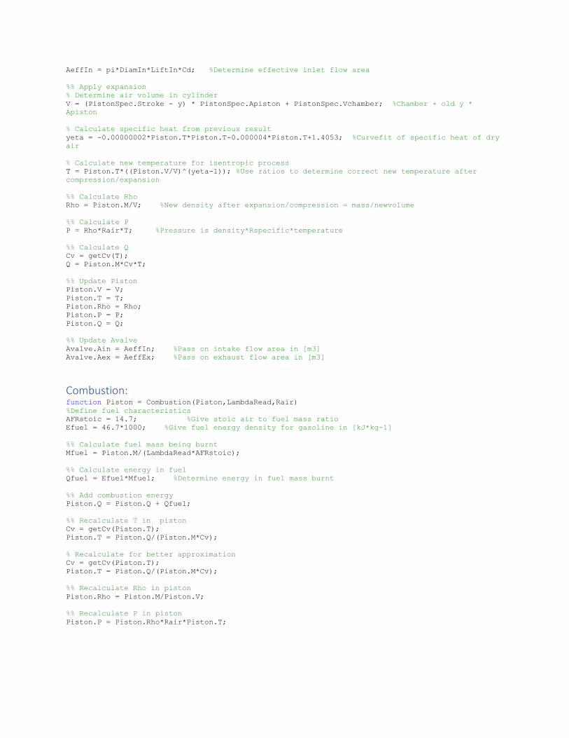
AeffIn = pi*DiamIn*LiftIn*Cd; %Determine effective inlet flow area

%% Apply expansion

% Determine air volume in cylinder

V = (PistonSpec.Stroke - y) * PistonSpec.Apiston + PistonSpec.Vchamber; %Chamber + old y *

Apiston

% Calculate specific heat from previous result

yeta = -0.00000002*Piston.T*Piston.T-0.000004*Piston.T+1.4053; %Curvefit of specific heat of dry

air

% Calculate new temperature for isentropic process

T = Piston.T*((Piston.V/V)^(yeta-1)); %Use ratios to determine correct new temperature after

compression/expansion

%% Calculate Rho

Rho = Piston.M/V; %New density after expansion/compression = mass/newvolume

%% Calculate P

P = Rho*Rair*T; %Pressure is density*Rspecific*temperature

%% Calculate Q

Cv = getCv(T);

Q = Piston.M*Cv*T;

%% Update Piston

Piston.V = V;

Piston.T = T;

Piston.Rho = Rho;

Piston.P = P;

Piston.Q = Q;

%% Update Avalve

Avalve.Ain = AeffIn; %Pass on intake flow area in [m3]

Avalve.Aex = AeffEx; %Pass on exhaust flow area in [m3]

Combustion: function Piston = Combustion(Piston,LambdaRead,Rair)

%Define fuel characteristics

AFRstoic = 14.7; %Give stoic air to fuel mass ratio

Efuel = 46.7*1000; %Give fuel energy density for gasoline in [kJ*kg-1]

%% Calculate fuel mass being burnt

Mfuel = Piston.M/(LambdaRead*AFRstoic);

%% Calculate energy in fuel

Qfuel = Efuel*Mfuel; %Determine energy in fuel mass burnt

%% Add combustion energy

Piston.Q = Piston.Q + Qfuel;

%% Recalculate T in piston

Cv = getCv(Piston.T);

Piston.T = Piston.Q/(Piston.M*Cv);

% Recalculate for better approximation

Cv = getCv(Piston.T);

Piston.T = Piston.Q/(Piston.M*Cv);

%% Recalculate Rho in piston

Piston.Rho = Piston.M/Piston.V;

%% Recalculate P in piston

Piston.P = Piston.Rho*Rair*Piston.T;

Flow: function [Piston,Plenum,Flows] = Flow(Piston,Avalve,Plenum,Athmos,TimeStep,Rair,Aefftb)

%Intialize flow

Flows.In = 0;

Flows.Ex = 0;

%Determine valve flow for all pistons

for i = 1:length(Piston)

%% Calculate intake port <> plenum flow

if Plenum.P > Piston(i).P

%Flow Plenum -> Piston

Mflow = Avalve(i).Ain*sqrt(2*Plenum.Rho*(Plenum.P-Piston(i).P)); %Determine mass

flow

Mflow = TimeStep*Mflow; %Determine resulting

Delta mass

%Get Cv

CvPlenum = getCv(Plenum.T);

%Determine Q changes

Plenum.Q = Plenum.Q - Mflow*CvPlenum*Plenum.T; %Remove energy from plenum

Piston(i).Q = Piston(i).Q + Mflow*CvPlenum*Plenum.T; %Add it to the piston

%Determine M changes

Plenum.M = Plenum.M - Mflow; %Remove mass from plenum

Piston(i).M = Piston(i).M + Mflow; %Add mass to piston

%Store intake flow

Flows(i).In = Mflow;

elseif Plenum.P < Piston(i).P

%Flow Piston -> Plenum

Mflow = Avalve(i).Ain*sqrt(2*Piston(i).Rho*(Piston(i).P-Plenum.P)); %Determine mass

flow

Mflow = TimeStep*Mflow; %Determine resulting Delta

mass

%Determine Cv

CvPiston = getCv(Piston(i).T);

%Determine Q changes

Piston(i).Q = Piston(i).Q - Mflow*CvPiston*Piston(i).T; %Remove Energy from piston

Plenum.Q = Plenum.Q + Mflow*CvPiston*Piston(i).T; %Add it to the plenum

%Determine M changes

Piston(i).M = Piston(i).M - Mflow; %Remove mass from piston

Plenum.M = Plenum.M + Mflow; %Add mass to plenum

%Store intake flow

Flows(i).In = -Mflow;

end

%% Calculate exhaust port <> athmosphere flow

if Athmos.P > Piston(i).P

%Flow Athmos -> Piston

Mflow = Avalve(i).Aex*sqrt(2*Athmos.Rho*(Athmos.P-Piston(i).P)); %Determine mass

flow

Mflow = TimeStep*Mflow; %Determine

resulting Delta mass

%Determine Cv

CvAthmos = getCv(Athmos.T);

%Determine Q changes

Piston(i).Q = Piston(i).Q + Mflow*CvAthmos*Athmos.T; %Add Energy to the piston

%Determine M changes

Piston(i).M = Piston(i).M + Mflow; %Add mass to piston

%Store exhaust flow

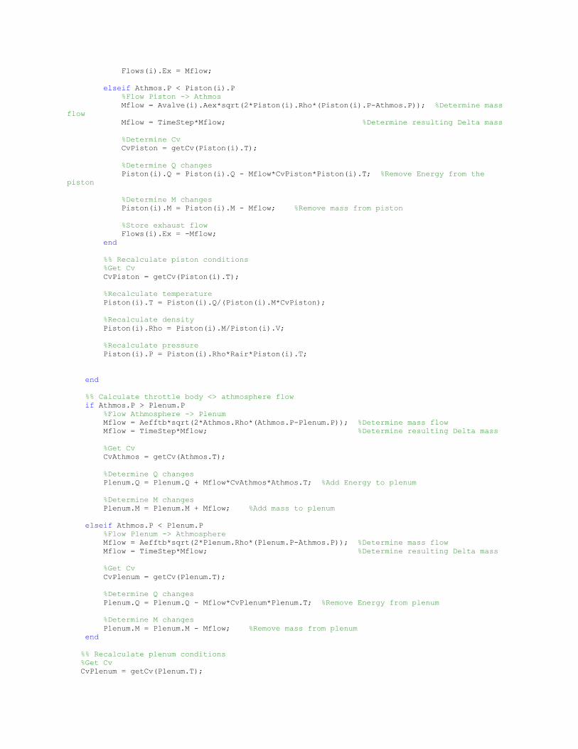
Flows(i).Ex = Mflow;

elseif Athmos.P < Piston(i).P

%Flow Piston -> Athmos

Mflow = Avalve(i).Aex*sqrt(2*Piston(i).Rho*(Piston(i).P-Athmos.P)); %Determine mass

flow

Mflow = TimeStep*Mflow; %Determine resulting Delta mass

%Determine Cv

CvPiston = getCv(Piston(i).T);

%Determine Q changes

Piston(i).Q = Piston(i).Q - Mflow*CvPiston*Piston(i).T; %Remove Energy from the

piston

%Determine M changes

Piston(i).M = Piston(i).M - Mflow; %Remove mass from piston

%Store exhaust flow

Flows(i).Ex = -Mflow;

end

%% Recalculate piston conditions

%Get Cv

CvPiston = getCv(Piston(i).T);

%Recalculate temperature

Piston(i).T = Piston(i).Q/(Piston(i).M*CvPiston);

%Recalculate density

Piston(i).Rho = Piston(i).M/Piston(i).V;

%Recalculate pressure

Piston(i).P = Piston(i).Rho*Rair*Piston(i).T;

end

%% Calculate throttle body <> athmosphere flow

if Athmos.P > Plenum.P

%Flow Athmosphere -> Plenum

Mflow = Aefftb*sqrt(2*Athmos.Rho*(Athmos.P-Plenum.P)); %Determine mass flow

Mflow = TimeStep*Mflow; %Determine resulting Delta mass

%Get Cv

CvAthmos = getCv(Athmos.T);

%Determine Q changes

Plenum.Q = Plenum.Q + Mflow*CvAthmos*Athmos.T; %Add Energy to plenum

%Determine M changes

Plenum.M = Plenum.M + Mflow; %Add mass to plenum

elseif Athmos.P < Plenum.P

%Flow Plenum -> Athmosphere

Mflow = Aefftb*sqrt(2*Plenum.Rho*(Plenum.P-Athmos.P)); %Determine mass flow

Mflow = TimeStep*Mflow; %Determine resulting Delta mass

%Get Cv

CvPlenum = getCv(Plenum.T);

%Determine Q changes

Plenum.Q = Plenum.Q - Mflow*CvPlenum*Plenum.T; %Remove Energy from plenum

%Determine M changes

Plenum.M = Plenum.M - Mflow; %Remove mass from plenum

end

%% Recalculate plenum conditions

%Get Cv

CvPlenum = getCv(Plenum.T);

%Recalculate temperature

Plenum.T = Plenum.Q/(Plenum.M*CvPlenum);

%Recalculate density

Plenum.Rho = Plenum.M/Plenum.V;

%Recalculate pressure

Plenum.P = Plenum.Rho*Rair*Plenum.T;

G5 – Combustion engine model operation overview Overview of model loop used for combustion engine model

F-G5 – Summary of operation of combustion engine model

Appendix H Observations for measurement and model results

Appendix H will consist of observations based upon the comparison of the measurements versus the

engine model. This section of the appendix will contain of the following:

H1: Comparison of FFT (Frequency Spectra)

H2: Comparison of Harmonics

H3: Comparison of Temperatures

Appendix H1 – FFT comparison Below the result of the frequency spectra measured and simulated can be found, along

with a brief description of relevant observations and notes.

1000 rpm 𝑓𝑝𝑒𝑎𝑘 1 [𝐻𝑧] 𝑓𝑝𝑒𝑎𝑘 2 [𝐻𝑧] 𝑓𝑝𝑒𝑎𝑘 3[𝐻𝑧] Brief description of observed results

Measurement long 33.2 64.9 98.0* Peak for measurement at 0.6 Hz

ignored since this is probably the

drive throttle position control error,

and far from the expected frequency

range for engine condition

characterization.

Model long 32.8 65.6 98.3

Deviation in % 1.2% -1.1% -0.3%

Deviation in ratio 1.01 0.99 1.00

T-H1.1 – Summary of frequency spectrum results of F-D1, with observation notes and frequency peak deviation in percentage and ratio. *estimate from graphs provided

1500 rpm 𝑓𝑝𝑒𝑎𝑘 1 [𝐻𝑧] 𝑓𝑝𝑒𝑎𝑘 2 [𝐻𝑧] 𝑓𝑝𝑒𝑎𝑘 3[𝐻𝑧] Brief description of observed results

Measurement long 52.6 106.5 160.0* Peak for measurement at 0.8 Hz

ignored since this is probably the drive

throttle position control error, and far

from the expected frequency range for

engine condition characterization.

Model long 52.0 104.0 156.0

Deviation in % 1.1% 2.3% 2.5%

Deviation in ratio 1.01 1.02 1.03

T-H1.2 – Summary of frequency spectrum results of F-D2, with observation notes and frequency peak deviation in percentage and ratio. *estimate from graphs provided

2000 rpm 𝑓𝑝𝑒𝑎𝑘 1 [𝐻𝑧] 𝑓𝑝𝑒𝑎𝑘 2 [𝐻𝑧] 𝑓𝑝𝑒𝑎𝑘 3[𝐻𝑧] Brief description of observed results

Measurement long 68.7 138.2 207.4 Measurement and model deviate in

slight manner, deviation ratio can also

be seen as relatively stable.

Model long 67.5 135.0 202.6

Deviation in % 1.7% 2.3% 2.3%

Deviation in ratio 1.02 1.02 1.02 T-H1.3 – Summary of frequency spectrum results of F-D3, with observation notes and frequency peak deviation in percentage and ratio.

2500 rpm 𝑓𝑝𝑒𝑎𝑘 1 [𝐻𝑧] 𝑓𝑝𝑒𝑎𝑘 2 [𝐻𝑧] 𝑓𝑝𝑒𝑎𝑘 3[𝐻𝑧] Brief description of observed results

Measurement long 85.0 170.0 151.5 In measurement additional peaks next to main frequency are observed. Third harmonic no longer within measurement range for sample rate.

Model long 85.0 170.0 -

Deviation in % 0.0% 0.0% -

Deviation in ratio 1.00 1.00 - T-H1.4 – Summary of frequency spectrum results of F-D4, with observation notes and frequency peak deviation in percentage and ratio.

3000 rpm 𝑓𝑝𝑒𝑎𝑘 1 [𝐻𝑧] 𝑓𝑝𝑒𝑎𝑘 2 [𝐻𝑧] 𝑓𝑝𝑒𝑎𝑘 3[𝐻𝑧] Brief description of observed results

Measurement long 102.3 203.7 60.3 Once more an additional peak is shown next to main peak of expected measurement frequency.

Model long 102.2 204.4 -

Deviation in % 0.1% -0.3% -

Deviation in ratio 1.00 1.00 - T-H1.5 – Summary of frequency spectrum results of F-D5, with observation notes and frequency peak deviation in percentage and ratio.

3500 rpm 𝑓𝑝𝑒𝑎𝑘 1 [𝐻𝑧] 𝑓𝑝𝑒𝑎𝑘 2 [𝐻𝑧] 𝑓𝑝𝑒𝑎𝑘 3[𝐻𝑧] Brief description of observed results

Measurement long 122.1 129.0 6.9 Additional frequency peak next to expected frequency observed once more. A strong oscillation can also be seen at 6.9 Hz, which is too fast for driver input, which is also observed in the model.

Model long 120.4 240.9 6.0

Deviation in % 1.4% -86.7% -

Deviation in ratio 1.01 0.54 -

T-H1.6 – Summary of frequency spectrum results of F-D6, with observation notes and frequency peak deviation in percentage and ratio.

4000 rpm 𝑓𝑝𝑒𝑎𝑘 1 [𝐻𝑧] 𝑓𝑝𝑒𝑎𝑘 2 [𝐻𝑧] 𝑓𝑝𝑒𝑎𝑘 3[𝐻𝑧] Brief description of observed results

Measurement long 130.8 85.8 50.0* Once more additional peaks next to main peak are observed. 0.2 Hz peak also observed but ignored since assumed user throttle input. Third harmonic now fully out of measurement range for sample rate.

Model long 134.4 8.0* -

Deviation in % -2.8% 90.7% -

Deviation in ratio 0.97 10.73 -

T-H1.7 – Summary of frequency spectrum results of F-D7, with observation notes and frequency peak deviation in percentage and ratio. *estimate from graphs provided

4500 rpm 𝑓𝑝𝑒𝑎𝑘 1 [𝐻𝑧] 𝑓𝑝𝑒𝑎𝑘 2 [𝐻𝑧] 𝑓𝑝𝑒𝑎𝑘 3[𝐻𝑧] Brief description of observed results

Measurement long 153.5 35.8 230.2 The expected main frequency peak is observed, with an additional 35.8 Hz peak. Also an additional peak at 230Hz observed.

Model long 150.8 8.0* -

Deviation in % 1.8% 77.7% -

Deviation in ratio 1.02 4.48 - T-H1.8 – Summary of frequency spectrum results of F-D8, with observation notes and frequency peak deviation in percentage and ratio. *estimate from graphs provided

5000 rpm 𝑓𝑝𝑒𝑎𝑘 1 [𝐻𝑧] 𝑓𝑝𝑒𝑎𝑘 2 [𝐻𝑧] 𝑓𝑝𝑒𝑎𝑘 3[𝐻𝑧] Brief description of observed results

Measurement long 169.8 15.5 85.0* Additional peak at 15Hz observed, which is also observed in model, undetermined peak observed at 85Hz.

Model long 152.5 10.0* -

Deviation in % 10.2% 35.5% -

Deviation in ratio 1.11 1.55 - T-H1.9 – Summary of frequency spectrum results of F-D9, with observation notes and frequency peak deviation in percentage and ratio. *estimate from graphs provided

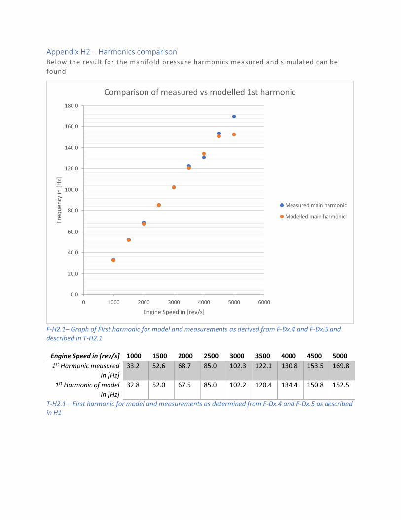
Appendix H2 – Harmonics comparison Below the result for the manifold pressure harmonics measured and simulated can be

found

F-H2.1– Graph of First harmonic for model and measurements as derived from F-Dx.4 and F-Dx.5 and described in T-H2.1

Engine Speed in [rev/s] 1000 1500 2000 2500 3000 3500 4000 4500 5000

1st Harmonic measured

in [Hz]

33.2 52.6 68.7 85.0 102.3 122.1 130.8 153.5 169.8

1st Harmonic of model

in [Hz]

32.8 52.0 67.5 85.0 102.2 120.4 134.4 150.8 152.5

T-H2.1 – First harmonic for model and measurements as determined from F-Dx.4 and F-Dx.5 as described in H1

0.0

20.0

40.0

60.0

80.0

100.0

120.0

140.0

160.0

180.0

0 1000 2000 3000 4000 5000 6000

Freq

uen

cy in

[H

z]

Engine Speed in [rev/s]

Comparison of measured vs modelled 1st harmonic

Measured main harmonic

Modelled main harmonic

F-H2.2– Graph of Second harmonic for model and measurements as derived from F-Dx.4 and F-Dx.5 and described in T-H2.2

Engine Speed in [rev/s] 1000 1500 2000 2500 3000 3500

2nd Harmonic measured in [Hz] 64.9 106.5 138.2 170.0 203.7 -

2nd Harmonic of model in [Hz] 65.6 104.0 135.0 170.0 204.4 240.9

T-H2.2 – Second harmonic for model and measurements as determined from F-Dx.4 and F-Dx.5 as described in H1. *estimate from graphs provided

0.0

50.0

100.0

150.0

200.0

250.0

300.0

0 500 1000 1500 2000 2500 3000 3500 4000

Freq

uen

cy in

[H

z]

Engine Speed in [rev/s]

Comparison of measured vs modelled 2nd harmonic

Measured second harmonic

Modelled second harmonic

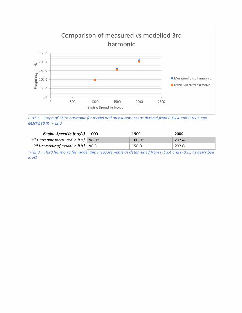
F-H2.3– Graph of Third harmonic for model and measurements as derived from F-Dx.4 and F-Dx.5 and described in T-H2.3

Engine Speed in [rev/s] 1000 1500 2000

3rd Harmonic measured in [Hz] 98.0* 160.0* 207.4

3rd Harmonic of model in [Hz] 98.3 156.0 202.6

T-H2.3 – Third harmonic for model and measurements as determined from F-Dx.4 and F-Dx.5 as described in H1

0.0

50.0

100.0

150.0

200.0

250.0

0 500 1000 1500 2000 2500

Freq

uen

cy in

[H

z]

Engine Speed in [rev/s]

Comparison of measured vs modelled 3rd harmonic

Measured third harmonic

Modelled third harmonic

Appendix H3 – Temperature Comparison Below the result for the engine temperatures measured and simulated can be found

F-H3.1 – Modelled and measured exhaust gas temperatures compared as taken from averages of Dx.2 and Dx.3, with air-fuel ratio for which was measured and simulated with included.

Engine Speed in [rev/s] 1000 1500 2000 2500 3000 3500 4000 4500 5000

Modelled EGT in [°C] 428.5 446.3 443.1 464.2 463.4 469.7 473.9 476.4 497.1

Measured EGT in [°C] 694.2 694.5 714.3 735.2 760.9 755.2 754.5 767.7 748.8

Air Fuel ratio (Lambda) 1.057 1.052 1.051 0.967 0.930 0.951 0.967 0.970 0.967

T-H3.1 Modelled and measured exhaust gas temperatures compared as taken from averages of Dx.2 and Dx.3, with air-fuel ratio for which was measured and simulated with included.

F-H3.2 – Modelled and measured manifold air temperatures compared as taken from averages of Dx.2 and Dx.3, with air-fuel ratio for which was measured and simulated with included.

Engine Speed in [rev/s] 1000 1500 2000 2500 3000 3500 4000 4500 5000

Modelled MAT in [°C] 83.9 138.8 159.7 164.9 175.7 173.3 171.7 171.1 161.9

Measured MAT in [°C] 21.5 25.3 28.7 30.1 32.2 34.6 35.5 36.7 37.0

Air Fuel ratio (Lambda) 1.057 1.052 1.051 0.967 0.930 0.951 0.967 0.970 0.967

T-H3.2 Modelled and measured manifold air temperatures compared as taken from averages of Dx.2 and Dx.3, with air-fuel ratio for which was measured and simulated with included.

0.85

0.9

0.95

1

1.05

1.1

0

200

400

600

800

1000

Tem

per

atu

re in

[°C

]

Engine Speed in [rev/s]

Lambda versus Exhaust Gas Temperature

Measured EGT

Model EGT

Air Fuel ratio (Lambda)

0.85

0.9

0.95

1

1.05

1.1

0

50

100

150

200

Tem

per

atu

re in

[°C

]

Engine Speed in [rev/s]

Lambda versus Intake Temperature

Measured MAT

Model MAT

Air Fuel ratio (Lambda)