www.iap.uni-jena.de

Optical Design with Zemax

for PhD - Advanced

Seminar 20 : Additional topics

2019-04-03

Herbert Gross / Norman Worku

Winter term 2019

2

Preliminary Schedule

Assistent

No Date Subject Detailed content Yi Uwe

Her-

bert

1 17.10. Introduction

Zemax interface, menus, file handling, system description, editors, preferences,

updates, system reports, coordinate systems, aperture, field, wavelength, layouts,

diameters, stop and pupil, solves x

2 24.10. Basic Zemax handlingRaytrace, ray fans, paraxial optics, surface types, quick focus, catalogs, vignetting,

footprints, system insertion, scaling, component reversal x Ziyao

3 07.11.Properties of optical

systems

aspheres, gradient media, gratings and diffractive surfaces, special types of

surfaces, telecentricity, ray aiming, afocal systems x Ziyao

4 14.11. Aberrations Irepresentations, spot, Seidel, transverse aberration curves, Zernike wave

aberrations x Yi

5 21.11. Aberrations II Point spread function and transfer function x Yi

6 28.11. Optimization I algorithms, merit function, variables, pick up’s x Ziyao

7 05.12. Optimization II methodology, correction process, special requirements, examples x Ziyao

8 12.12. Advanced handlingslider, universal plot, I/O of data, material index fit, multi configuration, macro

language x Yi

9 09.01. Imaging Fourier imaging, geometrical images x Yi

10 16.01. Correction I Symmetry, field flattening, color correction x Ziyao

11 23.01. Correction II Higher orders, aspheres, freeforms, miscellaneous x Ziyao

12 30.01. Tolerancing I Practical tolerancing, sensitivity x Yi

13 06.02. Tolerancing II Adjustment, thermal loading, ghosts x Yi

14 13.02. Illumination IPhotometry, light sources, non-sequential raytrace, homogenization, simple

examples x Yi

15 20.02. Illumination II Examples, special components x Yi

16 27.02. Physical modeling I Gaussian beams, Gauss-Schell beams, general propagation, POP x Yi

17 13.03. Physical modeling II Polarization, Jones matrix, Stokes, propagation, birefringence, components x Yi

18 20.03. Physical modeling III Coatings, Fresnel formulas, matrix algorithm, types of coatings x Yi

19 27.03. Physical modeling IVScattering and straylight, PSD, calculation schemes, volume scattering, biomedical

applications x Yi

20 03.04. Additional topicsAdaptive optics, stock lens matching, index fit, Macro language, coupling Zemax-

Matlab / Python x x Yi

Lecturer

3

Contents

1. Coupling Zemax / Matlab

2. Index fit

3. Macro language

4. Stock lens matching

5. Adaptive optics

Matlab-OpticStudio coupling using ZOS API

Introduction to ZOS API

Connecting OpticStudio to Matlab

Building optical systems

Ray tracing methods

System analysis tools

Demonstration

Conclusion

4

Introduction to ZOS-API

ZOS-API – Zemax OpticStudio Application Program Interface

Collection of interface functions to allow external programs to

access

• System data, editors and analyses tools

Three operation modes

• Standalone application (Matlab, Python, C# and C++)

• Entirely working on external program

• OpticStudio runs in the background

• Interactive application (Matlab and Python)

• OpticStudio and external program run simultaneously and interact

• User extension (C#, C++)

• Build analysis tools and operands similar to the inbuilt ones

5

Connecting OpticStudio and Matlab

Initial template code comes with OpticStudio installation

• Programming tab ZOS-API.NET Application Builders MATLAB

Standalone Application or Interactive Extension.

Template code

• Initialize connection with OpticStudio

• If successful run application (custom code)

• Clean up connection

Saved in “...\Documents\Zemax\ZOS-API

Projects\MATLABZOSConnection”

6

Interactive extension

Create interactive extension template.

Start the interactive extension

• Programming tab ZOS-API.NET Applications Interactive

Extension.

• Run the template code from Matlab

7

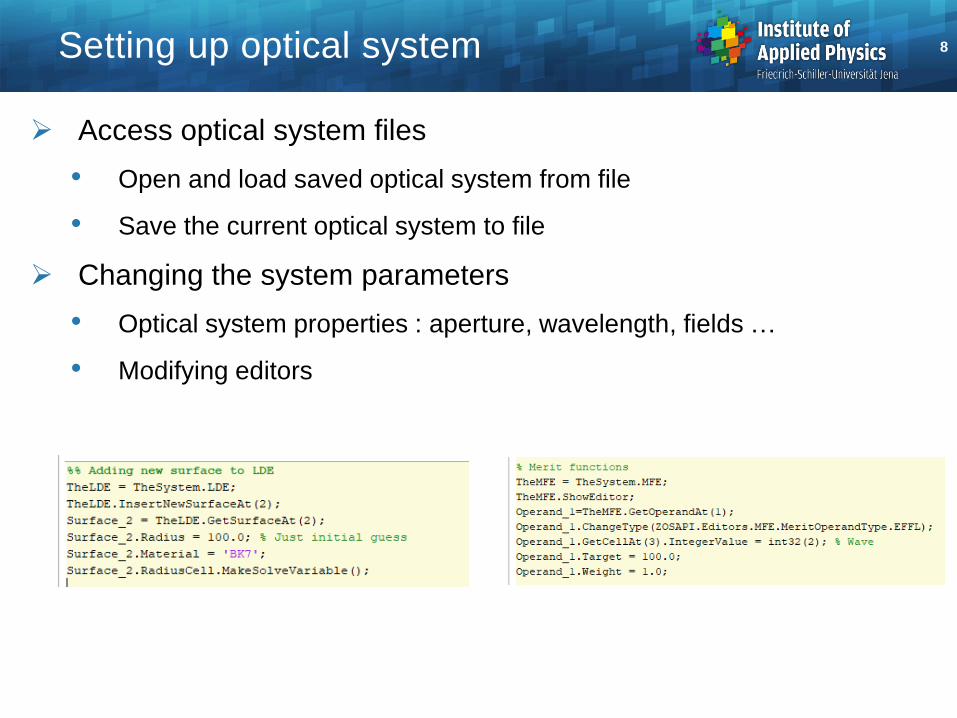
Setting up optical system

Access optical system files

• Open and load saved optical system from file

• Save the current optical system to file

Changing the system parameters

• Optical system properties : aperture, wavelength, fields …

• Modifying editors

8

Ray tracing

Trace rays through the system

• Single ray vs multiple rays (Batch ray trace)

• Normalized (ℎ𝑥, ℎ𝑦, 𝑝𝑥, 𝑝𝑦) vs direct (𝑥0, 𝑦0, 𝑧0, 𝑙0, 𝑚0, 𝑛0)

• Unpolarized vs polarized

• Batch ray tracer

• rayTracer = TheSystem.Tools.OpenBatchRayTrace();

• Multiple rays are traced at the same time

• Rays are added and results are read out individual with for loops

9

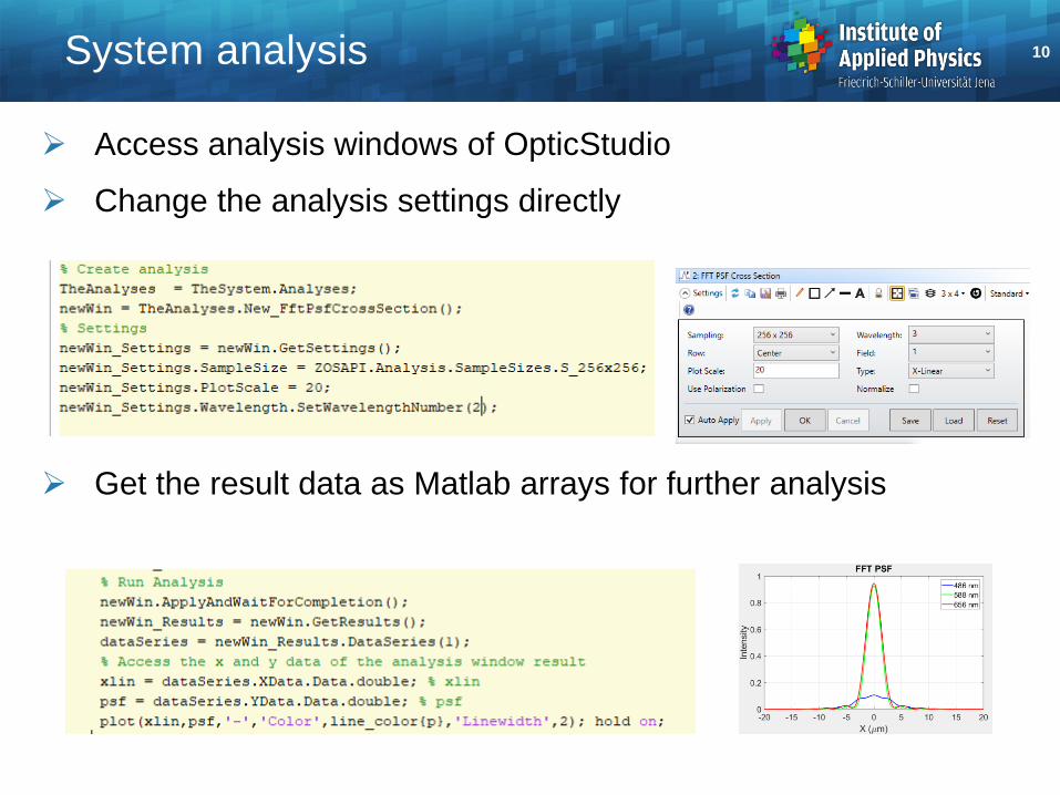
System analysis

Access analysis windows of OpticStudio

Change the analysis settings directly

Get the result data as Matlab arrays for further analysis

10

Conclusion

ZOS-API allows access of the OpticStudio from external

applications

Build optical systems

Trace multiple rays

Direct access to analysis settings and results

For more information

• User manual and ZOS-API syntax help

• Detailed description of the ZOS-API (classes, methods, properties, and

enumerated variables) with examples

• Sample codes for Matlab, Python, C++ and C#

• …\Documents\Zemax\ZOS-API Sample Code

11

Optional 4 glasses in comparison

12

Glass Dispersion

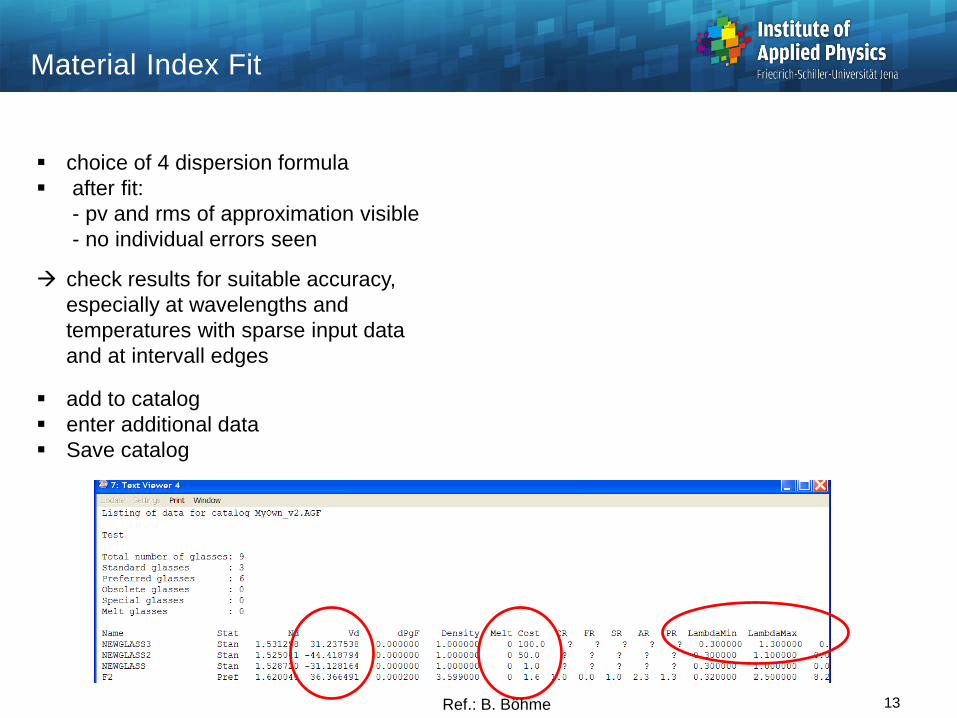
choice of 4 dispersion formula

after fit:

- pv and rms of approximation visible

- no individual errors seen

check results for suitable accuracy,

especially at wavelengths and

temperatures with sparse input data

and at intervall edges

add to catalog

enter additional data

Save catalog

Material Index Fit

13Ref.: B. Böhme

Establishing a special own

material

Select menue:

Tools / Catalogs / Glass catalogs

Options:

1. Fit index data

2. Fit melt data

Input of data for wavelengths

and indices

It is possible to establish own

material catalogs with additional

glasses as an individual library

14

Material Index Fit

Melt data:

- for small differences of real materials

- no advantage for new materials

Menue option:

‚Glass Fitting Tool‘

don‘t works (data input?)

15

Material Index Fit

Menue: Fit Index Data

Input of data: 2 options:

1. explicite entering wavelengths and indices

2. load file xxx.dat with two columns:

wavelength in mm and index

Choice of 4 different dispersion formulas

After fit:

- pv and rms of approximation visible

- no individual errors seen

- new material can be added to catalog

- data input can be saved to file

16

Material Index Fit

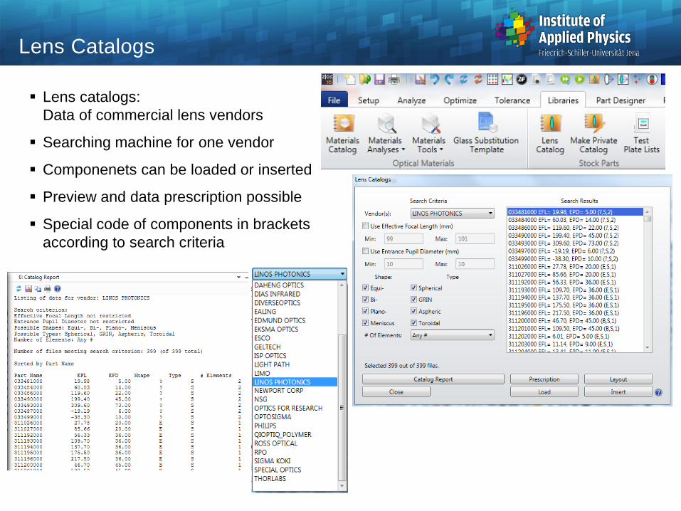
Lens catalogs:

Data of commercial lens vendors

Searching machine for one vendor

Componenets can be loaded or inserted

Preview and data prescription possible

Special code of components in brackets

according to search criteria

17

Lens Catalogs

Some system with more than one lens available

Sometimes:

- aspherical constants wrong

- hidden data with diameters, wavelengths,...

- problems with old glasses

Data stored in binary .ZMF format

Search over all catalogs not possible

Catalogs changes dynamically with every release

Private catalog can be generated

18

Lens Catalogs

Stock Lens Matching

This tool swaps out lenses in a design to the nearest equivalent candidate out of a

vendor catalogue

It works together with the merit function requirements (with constraints)

Aspheric, GRIN and toroidal surfaces not supported; only spherical

Works for single lenses and achromates

Compensation due to thickness adjustments is optional

Reverting a lens to optimize (?)

Top results are listed

Combination of best single lens substitutions is possible.

Overall optimization with nonlinear interaction ?

Ref.: D. Lokanathan

Stock Lens Matching

Selection of some vendors by

CNTR SHIFT marking

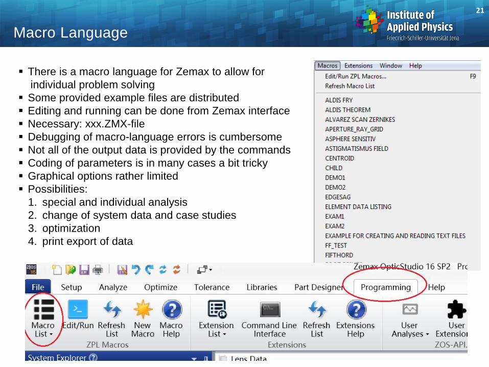
There is a macro language for Zemax to allow for

individual problem solving

Some provided example files are distributed

Editing and running can be done from Zemax interface

Necessary: xxx.ZMX-file

Debugging of macro-language errors is cumbersome

Not all of the output data is provided by the commands

Coding of parameters is in many cases a bit tricky

Graphical options rather limited

Possibilities:

1. special and individual analysis

2. change of system data and case studies

3. optimization

4. print export of data

21

Macro Language

Code Example:

Incidence angles at all surfaces

for 3 field positions

Online output

22

Macro Language

! comment line follows

variables, declarations, simple operations, strings, basic mathematical functions

IF THEN ELSE, GOTO, LABEL, FOR NEXT

a = AQVAL() numerical aperture

ro = CURV(j) surface curvature of surface no. j

y = FLDY(j) field size no. j

u = RAYL(j) direction cosine of real ray at surface no. j

y = RAYY(j) y-value of real ray at surface no. j

t = THIC(j) thickness at surface j

PRINT ‚text‘, x,y print text

FORMAT 5.3 numerical format of output: 5 places, 3 digits

OUTPUT ‚fname.txt‘ declaration of output file for results

GETSYSTEMDATA n get special coded (n) data of the system

GETZERNIKE maxorder, wave, field, sampling, vector, zerntype, epsilon, reference

PWAV n set primary wavelength

RAYTRACE hx, hy, px, py, wavelength

SURP surface, code, value1, value2 set surface properties

SYSP code, value1, value2 set system properties

23

Important Macro Commands

Calculate Focal lengths of all lenses

24

Macro Example 1 ! get number of surfaces Ns

Ns = nsur()

declare N, double, 1, Ns+1

! get refractive indices

FOR j = 1,Ns+1,1

N(j) = indx(j-1)

next

! number of lenses

Nl = 0

for j=1,Ns+1,1

if ( N(j) > 1 ) then Nl = Nl + 1

next

! header line: number of surfaces and glasses

print " "

format 2.0

print "lenses ",Nl

! focal lengths

print "focal lengths "

print " "

! print result

k=0

for j = 1 ,Ns-1,1

if ( N(j) == 1 ) then goto 1

k = k+1

c1 = curv(j-1)

c2 = curv(j)

t = thic(j-1)

ni = N(j)

F = (ni-1)*(c1-c2) + (ni-1)*(ni-1)/ni*t*c1*c2

foc = 0

if (F != 0) then foc = 1/F

format 2.0

print "L ",k," (",j-1,"-",j,") f = ",

format 10.4

print foc

label 1

next

Calculate telecentricity error

25

Macro Example 2

! sampling number over field

nfield = 21

! Set primary wavelength

jwave = pwav()

! define considered field index

jfield = 2

! save old field heigth

hyold = FLDY(jfield)

! calculate field increment

dw = 1/(nfield-1)

! fix ray data in pupil and x-field

hx = 0

px = 0

py = 0

! define surface of evaluation

n = nsur()

! header line

print " w-rel w-abs ws"

! raytrace of chief rays for all field heights and print results

FOR j = 1,nfield,1

hy = (j-1) * dw

hyabs = (j-1) * dw * hyold

SYSP 103, jfield, hy

update

raytrace hx, hy, px, py, jwave

delw = raym(n)

FORMAT 10.5

PRINT hy, hyabs, delw

NEXT

! recover data

SYSP 103, jfield, hyold

Calculate absolute size of Zernike

for astigmatism and coma

26

Macro Example 3

! Optional Output-File

!

! OUTPUT "c:\gross\new\zernvswave.txt"

!

! Number of points in the wavelength grid

!

jfield = 2

jwave = 1

!

! 1 = 32 , 2 = 64 Sampling Pupille

!

sampl = 2

maxzern = 9

!

! Set primary wavelength

!

wold = wavl(1)

!

! calculate Zernikes

!

GETZERNIKE maxzern,jwave, 1 ,sampl ,1, 0

ast = sqrt( vec1(8+5)*vec1(8+5) + vec1(8+6)*vec1(8+6) )

coma = sqrt( vec1(8+7)*vec1(8+7) + vec1(8+8)*vec1(8+8) )

!

! print result

!

print " "

FORMAT 10.5

PRINT "astig : ", ast

print "coma : ", coma

27

Example - 1

! 2013-05-12 H.Gross

!

! Calculation of the 2nd moments in x-and y-direction of a system spots for all field points

! A circular pupil shape is assumed

! number of field positions in the data

nfield = nfld()

!

! number of pupil sampling points (fix), arbitrary choice, determines accuracy and run time

!

npup = 21

! look for main wavelength in the data

!

jwave = pwav()

! initialization of increments in field and pupil

!

dw = 2/(nfield-1)

dp = 2/(npup-1)

!

! determine the index of image surface

n = nsur()

!

! header row in output: nfield npup jwave

print " "

print "Spot 2nd order moments in my"

print " "

FORMAT 10.5

PRINT "Fields: ",nfield, " pupil sampling: ",npup," wavelength: ",wavl(jwave)

print " "

28

Example - 2

!-------------------------------------------------

!

! loop over field points in y-direction: index jy

!

for jy = 1, nfield, 1

hx = 0

hy = sqrt((jy-1)/(nfield-1))

!

!----------------------------------------------------

!

! first loop to calculate the centroid

!

! initialization of centroids and moments

!

xc = 0

yc = 0

Mx2 = 0

My2 = 0

Nray = 0

!

! loop over pupil points: indices kx, ky

!

for ky = 1, npup, 1

for kx = 1, npup, 1

px = -1+(kx-1)*dp

py = -1+(ky-1)*dp

29

Example - 3

! raytrace

raytrace hx, hy, px, py, jwave

xp = rayx(n)

yp = rayy(n)

!

! error case for rays outside circular pupil

ierr = raye()

pr = sqrt(px*px+py*py)

if ( pr > 1) then ierr = 1

!

! summation of 1st order moment to calculate the centroid in x and y

if (ierr == 0)

Nray = Nray+1

xc = xc + xp

yc = yc + yp

endif

!

! end of pupil loop

next

next

!

! final calculation of centroid coordinates xc,yc

xc = xc / Nray

yc = yc / Nray

!

! second loop over pupil for calculation of moments M2 and M3

! indices kx, ky

for ky=1, npup, 1

for kx = 1, npup, 1

30

Example - 4

px = -1+(kx-1)*dp

py = -1+(ky-1)*dp

! raytrace

raytrace hx, hy, px, py, jwave

xp = rayx(n)

yp = rayy(n)

! error case

ierr = raye()

pr = sqrt(px*px+py*py)

if ( pr > 1) then ierr = 1

! summation of moments, scaling from mm into my

if (ierr == 0)

Mx2 = Mx2 + (xp-xc)*(xp-xc)*1.e6

My2 = My2 + (yp-yc)*(yp-yc)*1.e6

endif

! end of pupil loops

next

next

! final calculation of moments for present field location and print of results

Mx2 = Mx2 / Nray / 3.14159

My2 = My2 / Nray / 3.14159

!

! determine field size

Hy = fldy(jy)

FORMAT 8.4

PRINT "Field: ",Hy," Nray = ",Nray," centroid xc = ",xc," Mx2 = ",Mx2

PRINT " "," "," centroid yc = ",yc," My2 = ",My2

print " "

!

! end of field loop

next

User defined surfaces are possible

A routine written in C or C++ must be provided as DLL

By linking the DLL, the raytrace can be performed through user defined surfaces

Debugging of wrong DLL‘s is cumbersome, there is limited support from the hotline

Runtime is quite fast

Best way to establish a DLL due to the specific interface:

modify a provided C-source-routine

31

DLL Links

General Scheme of Adaptive Systems

optical

system

wavefront

sensor

adaptive

mirror

output

signal

wavefront

reconstruc-

tion

influence

function

control

algorithm

observation

actuators

object

Adaptive correction:

1. Measurement of image quality

Example: wavefront sensing

2. Signal processing and reconstruction

3. Digital calculation of necessary system

changes for optimization

4. Control and change of variable

component

Adaptive corrected systems

Measurement of perturbed wavefront

Appropriate phase conjugation by deformable mirror

Basic Setup

wavefront sensor

adaptive

mirror

sensor with

corrected image

perturbed

wavefront

calculation of

correction

Different types of variable components show quite different behavior of support:

1. spatial support - binary, limited range, no crosstalk (SLM, pixelized)

- limited support (electrostatic membran mirrors)

- global support (thick membran mirror plate)

strong correlation

2. frequency support - band limited, high frequency (SLM)

- only low frequencies (mirror plate)

Considerable influence on the correctability:

1. Spatial frequency response (higher order correction)

2. Condition of optimization matrix

3. Speed of correction

4. Boundary bahaviour

5. Degrees of freedom

Influence Functions

Influenz functions of actuators of a deformable mirror

Shape changes with position on mirror due to boundary effects

Decomposition of the wavefront into basic influence functions

Typically strong overlap

Influence Functions

Different geometries of sensor and actuator

Large bandwidth of correlation matrix

Geometry of Sensor and Actuators

geometry of sensorgeometry of actuators and

extension of influence functionscoupling matrix

sensor array

xSj , ySj

cartesian

actuator array

xSj , ySj

hexagonal

Geometry of Sensor and Variable Component

Usually, there are two different arrays:

1. Sensor array, measurement of quality

2. Actuator array for changing the wave

Critical:

1. different geometries

2. interlace effects and Moire

3. Boundary ranges

4. different number of cells, bad

resolution match

Resolution and Correctability

Correctability as function of the number of actuators and wavefront sensors

Hexagonal geometry usually better

Equal spatial resolution are benefitial

Sqrt(Nact)

Strehl Ds

0 5 10 15 20 25 300

10

20

30

40

50

60

70

80

90

100

NWFS = 100

NWFS = 256

NWFS =400

NWFS =625

hexagonal

hexagonal

cartesian

cartesian

Correction by adaptive

mirror

Strehl ratio increased from

0.05 to 0.60

Boundary effects limit the

performance

Adaptive Correction

1) PSF perturbed2) PSF after correction

1) Phase perturbed: Wrms = 0.60 2) Phase corrected: Wrms = 0.20

Star image without and with adaptive correction

Example of Adaptive Correction in Astronomy