advanced fluid mechanics -...
TRANSCRIPT
Advanced Fluid Mechanics
Chapter1- 1
hy
x
FU
Fluid (e.g. water)
u(y) = y/h U
Chapter 1 Introduction 1.1 Classification of a Fluid (A fluid can only substain tangential force when it moves)
1.) By viscous effect: inviscid & Viscous Fluid. 2.) By compressible: incompressible & Compressible Fluid. 3.) By Mack No: Subsonic, transonic, Supersonic, and hypersonic flow. 4.) By eddy effect: Laminar, Transition and Turbulent Flow.
The objective of this course is to examine the effect of tangential (shearing) stresses on a fluid.
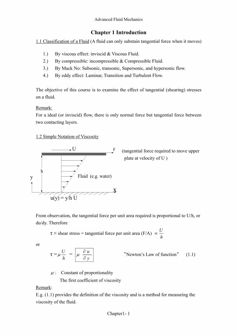
Remark: For a ideal (or inviscid) flow, there is only normal force but tangential force between two contacting layers. 1.2 Simple Notation of Viscosity (tangential force required to move upper
plate at velocity of U ) From observation, the tangential force per unit area required is proportional to U/h, or du/dy. Therefore
τ ≡ shear stress = tangential force per unit area (F/A) hU
∝
or
τ =hUµ =
yu
∂∂µ 〝Newton’s Law of function〞 (1.1)
µ : Constant of proportionality
The first coefficient of viscosity Remark: E.g. (1.1) provides the definition of the viscosity and is a method for measuring the viscosity of the fluid.

Advanced Fluid Mechanics
Chapter1- 2
In generally, if XYε represent the strain rate, then
( )xy xyfτ ε= (1.2)
τ
ε
Yield stress
plasticyielding fluids
Dilatent fluid Pesudoplastic fluid
Non- Newtonian fluid
Newtonian fluid
Newtonian fluid: linear relation between τ and ε
Pesudoplastic fluid: the slope of the curve decrease as ε increase (shear-thinning) of the shear-thinning effect is very strong. The fluid is called plastic fluid.
Dilatent fluid: the slope of the curve increases as ε increases (shear-thicking).
Yielding fluid: A material, part solid and part fluid can substain certain stresses before it starts to deform.
Note
1 Pa (Pascal) ≡ 2mNewton (Pascal, a French philosopher and Mathematist)
(a unit of pressure )
[µ] = [pa · sec] (= sm
smkg
⋅⋅
2
2 =
smkg⋅
= 10scm
g⋅
)
The metric unit of viscosity is called the poise (p) in honor of J.L.M. Poiseuille (1840), who conducted pioneering experiment on viscous flow in tubes.
1 P ≡ ( )( )scmg1
= 0.1 sec⋅pa

Advanced Fluid Mechanics
Chapter1- 3
The unit of viscosity:
[ ]µ =
∂yuατ =
LTL
LF
2=
T
LF
2 ← (Old -English Unit: F-L-T)
or
[ ]µ =
⋅T
LT
ML
2
2 =
LTM ← (international system SI unit: M-L-T)
Denote: 2MN ≡ Pa, then
sec1001.1 320, ⋅×=° Pacwaterµ
sec283100, ⋅=° Pacwaterµ
sec9.1720, ⋅=° Pacairµ
sec9.22100, ⋅=° Pacairµ
For dilute gas:
n
TT
≈
°°µµ
(Power- law)
STST
TT
++
≈ °
°°
23
µµ
(Sutherland’s law)
Where 0µ , 0T and S depends on the nature of the gases.
Kinematics Viscosity ρµυ ≡
(liquid): T → µ
(gas): T → µ

Advanced Fluid Mechanics
Chapter1- 4
θ∞U
R
uw
1
-3
Exp: (Effect of Viscosity on fluid) Flow past a cylinder Foe a ideal flow:
( )
−= ∞ 1cos, 2
2
rRUru θθ
( )
+= ∞ 1sin, 2
2
rRUrv θθ
At r = R, u=0, θsin2 ∞= Uv
The Bernoulli e.g. along the surface is:
pvPU +=+ ∞∞22
21
21 ρρ (Incompressible flow)
θρ
22
2
2sin
4111
21
−=−=−
=∞
∞
∞
Uv
U
PPC p
D’Albert paradox: No Drag. For a real flow: (viscous effect in)
µρVD
=Re
Re=0.16 (fig 6)(前後幾乎對稱)
( ) Re=1.54 (fig 24)前後不對稱

Advanced Fluid Mechanics
Chapter1- 5
Red ∼R eL ∼
(pair of recirculating eddies) Re=9.6 (fig 40) (6 < Re <40)
R=26 (fig. 26)d
L
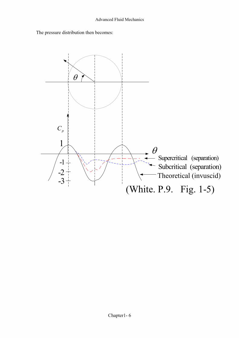
Separation occur
90θ > °
90sepθ < °
supercritical
Subcritical
Advanced Fluid Mechanics
Chapter1- 6
The pressure distribution then becomes:
θ
pC
θ
(White. P.9. Fig. 1-5)
Supercritical (separation)Subcritical (separation)Theoretical (invuscid)
-1
1
-2-3

Advanced Fluid Mechanics
Chapter1- 7
Remark: Newtonian Fluid Non-Newton Fluid
For a Newtonian fluid:
τ µ ε↔ ↔
= − τ↔
: stress tension
ε↔
: rate of strain tension
µ = a constant for a given temp, pressure and composition
Lf µ is not a constant for a given temp, pressure and composition, then the fluid is
called Non-Newtonian fluid. The Non-Newtonian fluid can be classified into several
kinds depending on how we model the viscosity. For example:
(I)Generalized Newtonian fluid
τ η ε↔ ↔
= − η = a function of the scalar invariants of ε↔
(i) The Carreau-Yusuda Model
( 1)
0
[1 ( ) ]n
a aη η λεη η
−∞
∞
−= +
− ε: magnitude of the ↔
ε
(ii) power-Law model
1−= nm εη
n<1: pseudo plastic (shear thinning) n=1: Newtonian fluid n>1: dilatant (shear thickening)
(II)Linear Viscoelastic Fluid → polymeric fluids (III)Non-linear Viscoelastic Fluid → The fluid has both 〝viscous〞 and 〝elastic〞 properties.
By 〝elasticity〞one usually means the ability of a material to return to some unique,
original shape on the other hand, by a 〝fluid〞, one means a material that will take the
shape of any container in which it is left, and thus does not possess a unique, original
shape. Therefore the viscoelastic fluid is often returned as 〝memory fluid〞.
Advanced Fluid Mechanics
Chapter1- 8
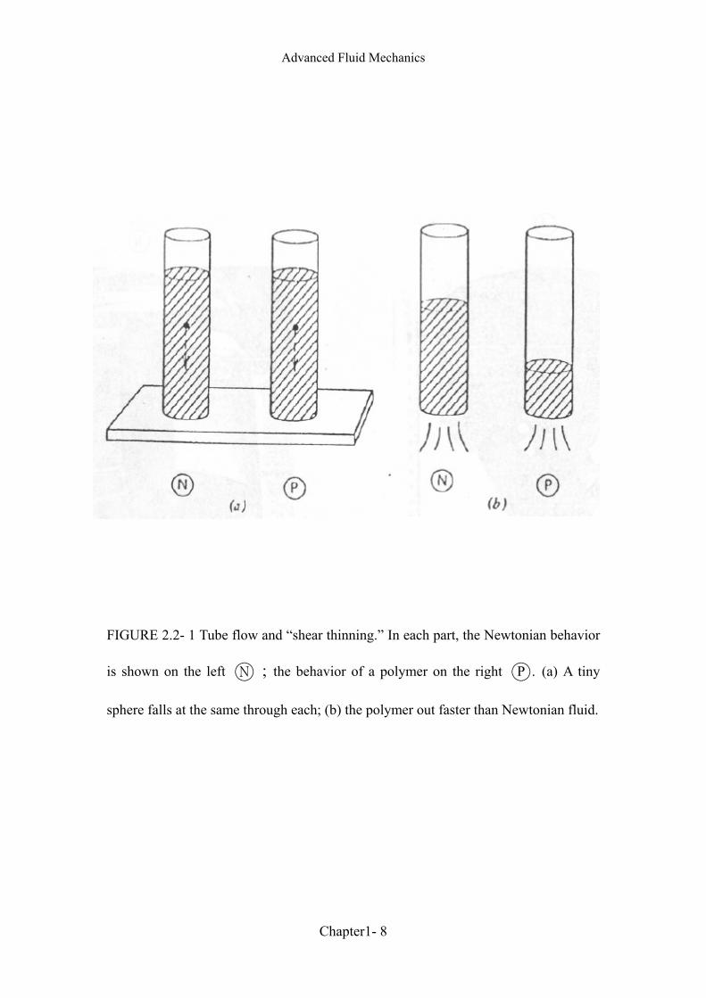
FIGURE 2.2- 1 Tube flow and “shear thinning.” In each part, the Newtonian behavior
is shown on the left N ; the behavior of a polymer on the right P . (a) A tiny
sphere falls at the same through each; (b) the polymer out faster than Newtonian fluid.
Advanced Fluid Mechanics
Chapter1- 9
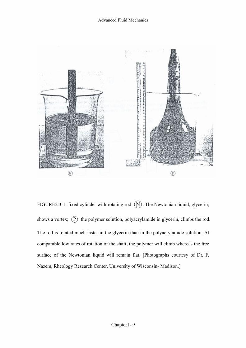
FIGURE2.3-1. fixed cylinder with rotating rod N . The Newtonian liquid, glycerin,
shows a vortex; P the polymer solution, polyacrylamide in glycerin, climbs the rod.
The rod is rotated much faster in the glycerin than in the polyacrylamide solution. At
comparable low rates of rotation of the shaft, the polymer will climb whereas the free
surface of the Newtonian liquid will remain flat. [Photographs courtesy of Dr. F.
Nazem, Rheology Research Center, University of Wisconsin- Madison.]
Advanced Fluid Mechanics
Chapter1- 10
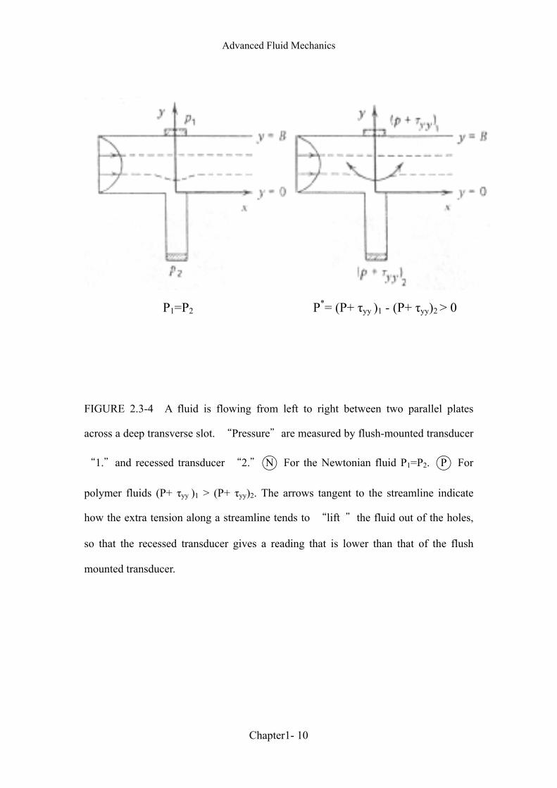
P1=P2 P*= (P+ τyy )1 - (P+ τyy)2 > 0
FIGURE 2.3-4 A fluid is flowing from left to right between two parallel plates
across a deep transverse slot. “Pressure”are measured by flush-mounted transducer
“1.”and recessed transducer “2.”N For the Newtonian fluid P1=P2. P For
polymer fluids (P+ τyy )1 > (P+ τyy)2. The arrows tangent to the streamline indicate
how the extra tension along a streamline tends to “lift ”the fluid out of the holes,
so that the recessed transducer gives a reading that is lower than that of the flush
mounted transducer.
Advanced Fluid Mechanics
Chapter1- 11
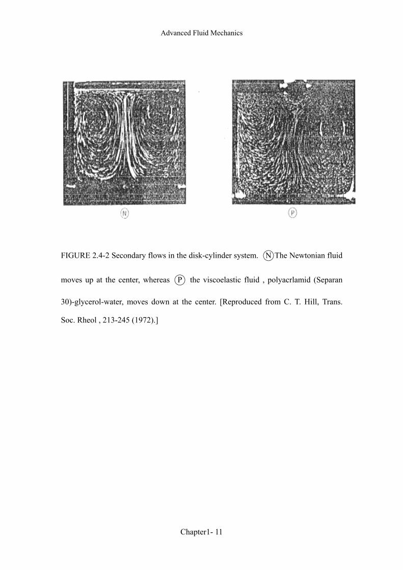
FIGURE 2.4-2 Secondary flows in the disk-cylinder system. N The Newtonian fluid
moves up at the center, whereas P the viscoelastic fluid , polyacrlamid (Separan
30)-glycerol-water, moves down at the center. [Reproduced from C. T. Hill, Trans.
Soc. Rheol , 213-245 (1972).]
Advanced Fluid Mechanics
Chapter1- 12
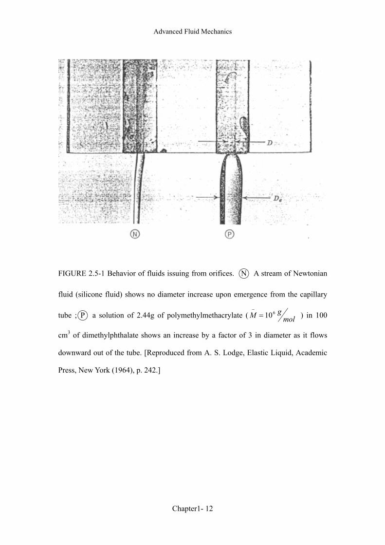
FIGURE 2.5-1 Behavior of fluids issuing from orifices. N A stream of Newtonian
fluid (silicone fluid) shows no diameter increase upon emergence from the capillary
tube ;P a solution of 2.44g of polymethylmethacrylate ( molgM 610=
−
) in 100
cm3 of dimethylphthalate shows an increase by a factor of 3 in diameter as it flows
downward out of the tube. [Reproduced from A. S. Lodge, Elastic Liquid, Academic
Press, New York (1964), p. 242.]

Advanced Fluid Mechanics
Chapter1- 13
FIGURE 2.5-2 the tubeless siphon. N When the siphon tube is lifted out of the
fluid, the Newtonian liquid stops flowing; P the macromolecular fluid continues to
be siphoned.
FIGURE 2.5-8 AN aluminum soap solution, made of aluminum dilaurate in decalin
and m-cresol, is (a) poured from a beaker and (b) cut in midstream. In (c), note that
the liquid above the cut springs back to the beaker and only the fluid below the cut
falls to the container.[Reproduced from A. S. Lodge, Elastic liquids, Academic Press,
New York (1964), p. 238. For a further discussion of aluminum soap solutions see N.
Weber and W. H. Bauer, J. Phys. Chem., 60, 270-273 (1956).]
Advanced Fluid Mechanics
Chapter1- 14
320 熱傳學
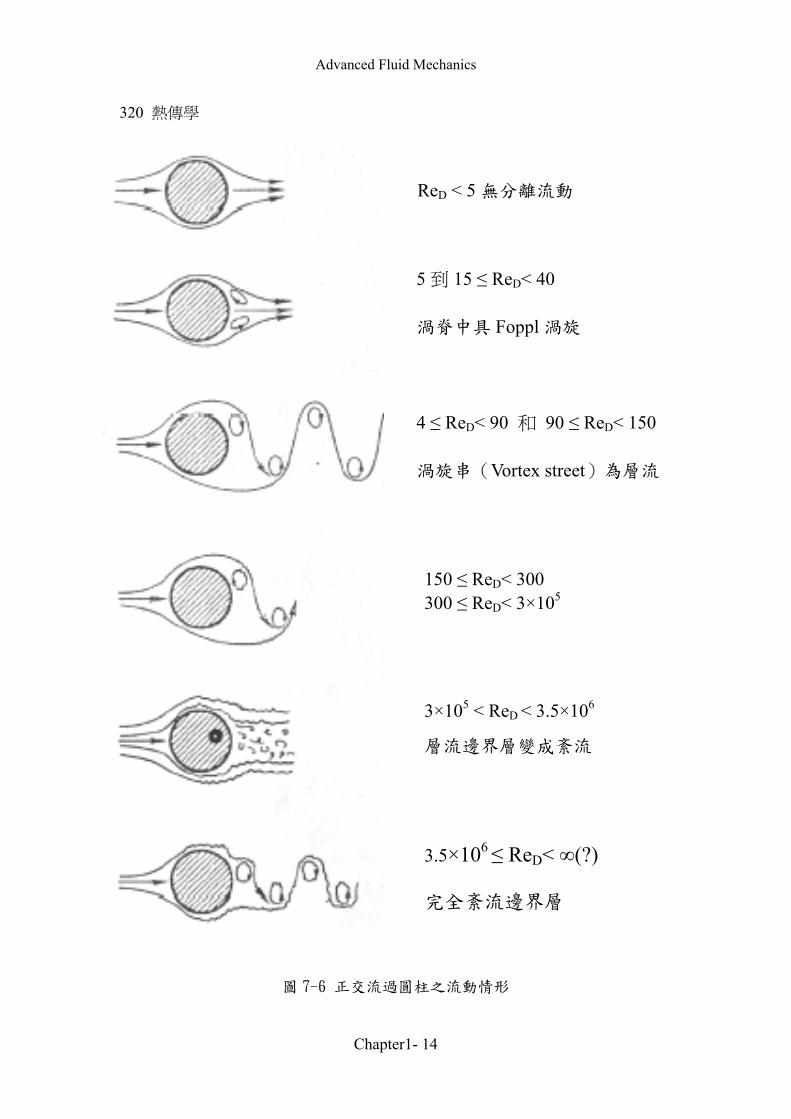
ReD < 5 無分離流動
圖 7-6 正交流過圓柱之流動情形
5 到 15 ≤ ReD< 40
渦脊中具 Foppl 渦旋
4 ≤ ReD< 90 和 90 ≤ ReD< 150
渦旋串(Vortex street)為層流
150 ≤ ReD< 300 300 ≤ ReD< 3×10⁵
3×10⁵ < ReD < 3.5×10⁶
層流邊界層變成紊流
3.5×10⁶ ≤ ReD< ∞(?)
完全紊流邊界層

Advanced Fluid Mechanics
Chapter1- 15
圖 7-7 長圓柱及球體之阻力係數 pC 與 Re 數關係
以下討論不同雷諾數下的物理現象:
(1) 雷諾數的數量級為 1或更小時,流場沒有分離現象,黏滯力是阻力的唯一
因素,此時流場可由勢流理論(Potential flow theory)來導證,在圖 7-7
中阻力係數隨著雷諾數的提高而直線變化下降。
(2) 雷諾數的數量級為 10 時,流場漸漸發生渦流,在圓柱後面有小渦旋
(Vertex) 出現,此時阻力的因素除了邊界層阻力外尚有渦流的因素,阻
力係數依雷諾數的提高而下降。
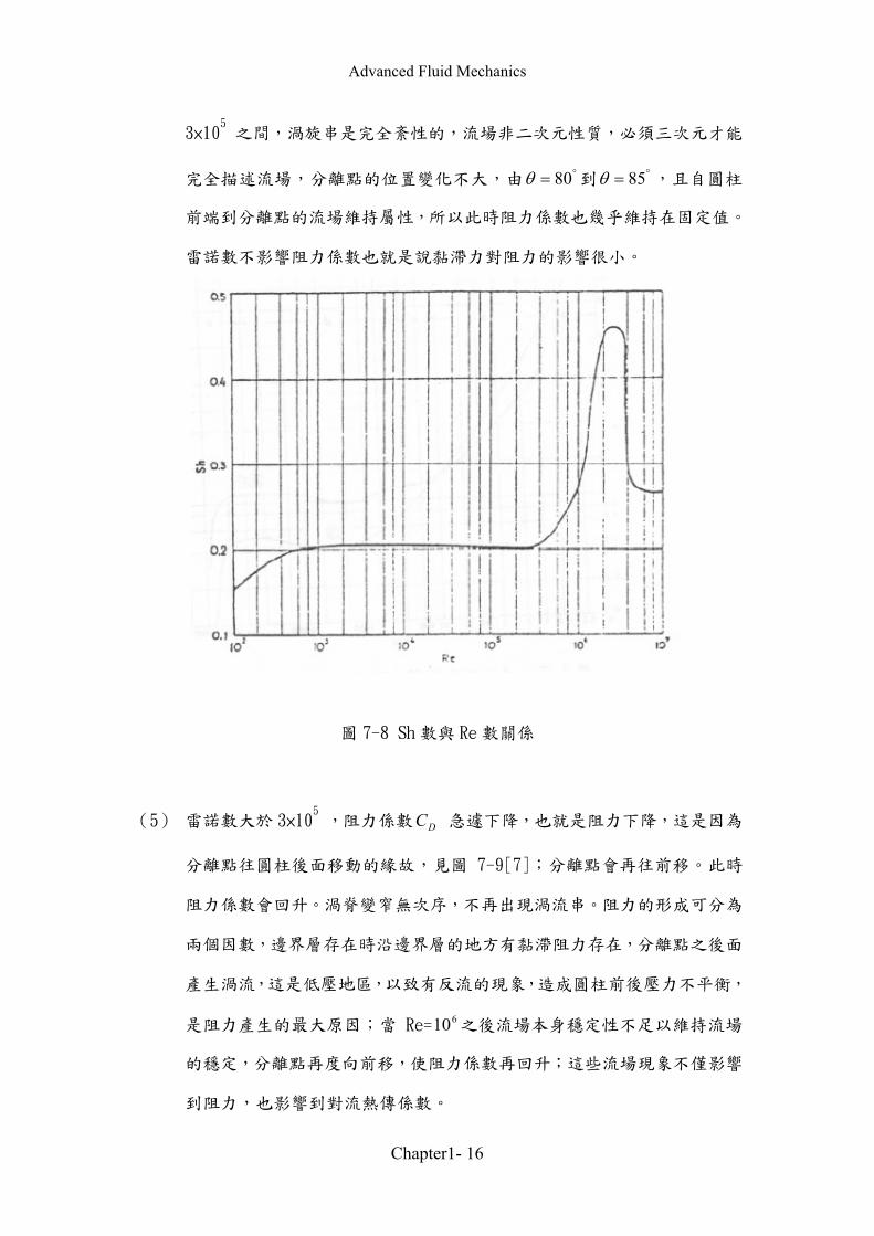
(3) 雷諾數介於 40 到 150 之間時,圓柱後形成渦旋串(Vertex street) ,產
生渦旋的頻率 fv 與流場雷諾數大小有關,定義 Strouhal 數 Sh:
∞
⋅=
uDf
Sh v (7-32)
Sh 與雷諾數 DRe 的關係如下圖 7-8;此時阻力主要由係由渦流造成。
(4) 雷諾數介於 150〜300 時,渦流串由層性漸漸轉變成紊性,雷諾數 300 到
Advanced Fluid Mechanics
Chapter1- 16
3×10⁵ 之間,渦旋串是完全紊性的,流場非二次元性質,必須三次元才能
完全描述流場,分離點的位置變化不大,由 °= 80θ 到 °= 85θ ,且自圓柱
前端到分離點的流場維持屬性,所以此時阻力係數也幾乎維持在固定值。
雷諾數不影響阻力係數也就是說黏滯力對阻力的影響很小。
圖 7-8 Sh 數與 Re 數關係
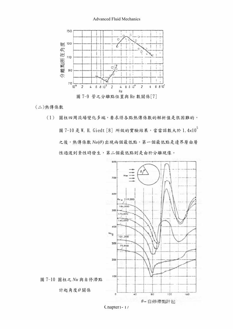
(5) 雷諾數大於 3×10⁵ ,阻力係數 DC 急遽下降,也就是阻力下降,這是因為
分離點往圓柱後面移動的緣故,見圖 7-9[7];分離點會再往前移。此時
阻力係數會回升。渦脊變窄無次序,不再出現渦流串。阻力的形成可分為
兩個因數,邊界層存在時沿邊界層的地方有黏滯阻力存在,分離點之後面
產生渦流,這是低壓地區,以致有反流的現象,造成圓柱前後壓力不平衡,
是阻力產生的最大原因;當 Re= 610 之後流場本身穩定性不足以維持流場
的穩定,分離點再度向前移,使阻力係數再回升;這些流場現象不僅影響
到阻力,也影響到對流熱傳係數。
Advanced Fluid Mechanics
Chapter1- 17
圖 7-9 管之分離點位置與 Re 數關係[7]
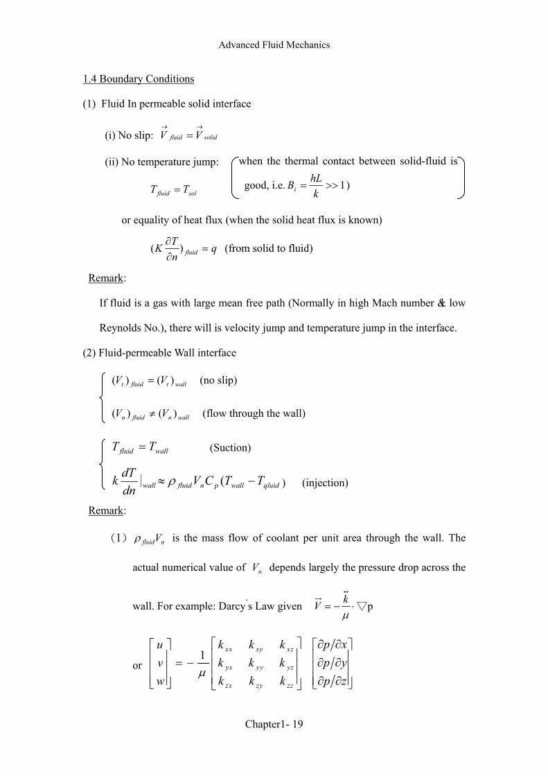
(二)熱傳係數
(1) 圓柱四周流場變化多端,要求得各點熱傳係數的解析值是很困難的,
圖 7-10 是 W. H. Giedt [8] 所做的實驗結果,當雷諾數大於 1.4×10⁵
之後,熱傳係數 )(θNu 出現兩個最低點,第一個最低點是邊界層由層
性過渡到紊性時發生,第二個最低點則是由於分離現像。
圖 7-10 圓柱之 Nu 與自停滯點
計起角度θ關係

Advanced Fluid Mechanics
Chapter1- 18
1.3 Properties of Fluids
There are four types of properties:
1. Kinematic properties
(Linear velocity, angular velocity, vorticity, acceleration, stain, etc.)
—strictly speaking, these are properties of the flow field itself rather than of the
fluid.
2. Transport properties
(Viscosity, thermal conductivity, mass diffusivity)
Transport phenomena:
Macroscopic cause Molecular Transport Macroscopic Reset
Non uniform flow velocity Momentum Viscosity
Non uniform flow temp Energy Heat conduction
Non uniform flow composition Mass Diffusion
e.g.:2
1
dudu
µτ = , 2dx
dTKg −= , 2dx
dxD A
ABA −=Γ
3. Thermodynamic properties
(pressure, density, temp, enthalpy, entropy, specific heat, prandtl number, bulk
modulus, etc)
—Classical thermodynamic, strictly speaking, does not apply to this subject, since
a viscous fluid in motion is technically not in equilibrium. However, deviations
from local thermodynamic equilibrium are usually not significient except when
flow residence time are short and the number of molecular particles, e.g.,
hypersonic flow of a rarefied gas.
4. Other miscellaneous properties
(surface tension, vapor pressure, eddy-diffusion coeff, surface-accommodation
coefficients, etc.)
Property is a point function, not a point function.
Advanced Fluid Mechanics
Chapter1- 19
1.4 Boundary Conditions
(1) Fluid In permeable solid interface
(i) No slip: solidfluid VV→→
=
(ii) No temperature jump:
solfluid TT =
or equality of heat flux (when the solid heat flux is known)
qnTK fluid =∂∂ )( (from solid to fluid)
Remark:
If fluid is a gas with large mean free path (Normally in high Mach number & low
Reynolds No.), there will is velocity jump and temperature jump in the interface.
(2) Fluid-permeable Wall interface
walltfluidt VV )()( = (no slip)
wallnfluidn VV )()( ≠ (flow through the wall)
wallfluid TT = (Suction)
qluidwallpnfluidwall TTCVdndTk −≈ (∣ ρ ) (injection)
Remark:
(1) nfluidVρ is the mass flow of coolant per unit area through the wall. The
actual numerical value of nV depends largely the pressure drop across the
wall. For example: Darcy’s Law given ⋅−=µkV p
or 1 xx xy xz
yx yy yz
zx zy zz
u k k kv k k kw k k k
µ
= −
p xp yp z
∂ ∂ ∂ ∂ ∂ ∂
when the thermal contact between solid-fluid is
good, i.e. 1>>=k
hLBi )
Advanced Fluid Mechanics
Chapter1- 20
),,( tyxηη =
Liquid, P Ry
x
z
Pa
Pa
P
P ( P<Pa)
( P>Pa)
interface(1)
(2)
Liquid
V
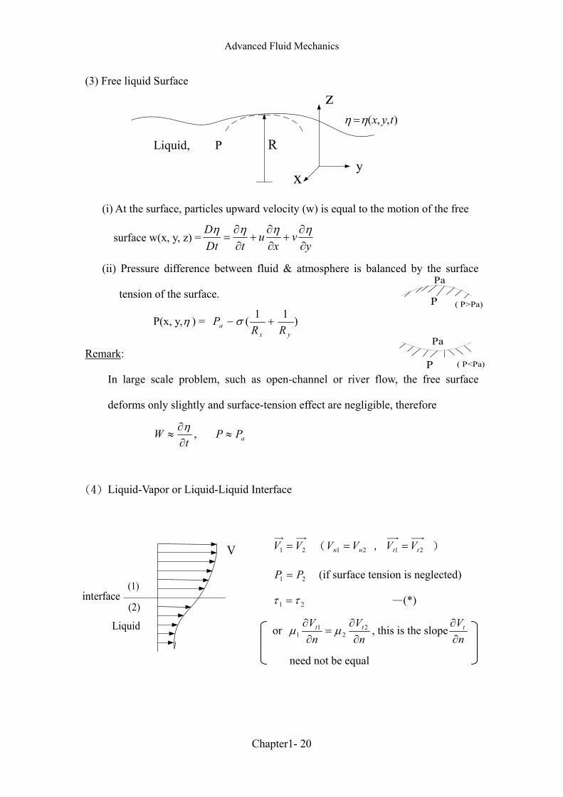
(3) Free liquid Surface
(i) At the surface, particles upward velocity (w) is equal to the motion of the free
surface w(x, y, z) =y
vx
utDt
D∂∂
+∂∂
+∂∂
=ηηηη
(ii) Pressure difference between fluid & atmosphere is balanced by the surface
tension of the surface.
P(x, y,η ) = )11(yx
a RRP +− σ
Remark:
In large scale problem, such as open-channel or river flow, the free surface
deforms only slightly and surface-tension effect are negligible, therefore
t
W∂∂
≈η , aPP ≈
(4) Liquid-Vapor or Liquid-Liquid Interface
21 VV = ( 21 nn VV = , 21 tt VV = )
21 PP = (if surface tension is neglected)
21 ττ = —(*)
or n
Vn
V tt
∂∂
=∂∂ 2
21
1 µµ , this is the slopenVt
∂∂
need not be equal

Advanced Fluid Mechanics
Chapter1- 21
interface(1)
(2)
T 21 TT =
21 qq = (Since interface has vanishing mass,
it can’t store momentum or energy.)
or nT
knT
k∂∂
−=∂∂
− 22
11 —(**)
Remark:
(1) If region (1) is vapor, itsµ & k are usually much smaller than for a liquid,
therefore, we may approximate E.g. (*) & (**) as
0)( ≈∂∂
liqt
nV
, 0)( ≈∂∂
liqnT
(2) If there is evaporation, condensation, or diffusion at the interface, the mass
flow must be balance, ⋅⋅
= 21 mm .
n
CDn
CD∂∂
=∂∂ 2
21
1
(5) Inlet and Exit Boundary Conditions
For the majority of viscous-flow analysis, we need to knowV , P, and T at every
point on inlet & exit section of the flow. However, through some approximation or
simplification, we can reduce the boundary condition s needed at exit.
Advanced Fluid Mechanics
Chapter1- 22
Supplementary Remarks
(1) Transports of momentum, energy, and mass are often similar and sometimes
genuinely analogous. The analogy fails in multidimensional problems become
heat and mass flux are vectors while momentum flux is a tension.
(2) Viscosity represents the ability of a fluid to flow freely. SAE30 means that 60 ml
of this oil at a specific temperature takes 30s to run out of a 1.76 cm hole in the
bottom of a cup.
(3) The flow of a viscous liquid out of the bottom of a cup is a difficult problem for
which no analytic solution exits at present.
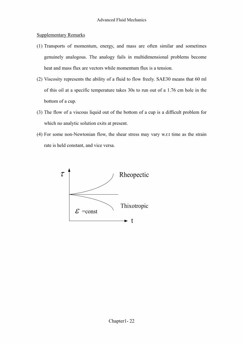
(4) For some non-Newtonian flow, the shear stress may vary w.r.t time as the strain
rate is held constant, and vice versa.
ε
τ Rheopectic
Thixotropic
t=const
Advanced Fluid Mechanics
Chapter1- 23
Advanced Fluid Mechanics
Chapter1- 24
Advanced Fluid Mechanics
Chapter1- 25
Advanced Fluid Mechanics
Chapter1- 26
Advanced Fluid Mechanics
Chapter2- 1
r!R
"!( , , )X Y Zy
x
0t =
z
(same particle)t>0(x, y, z)
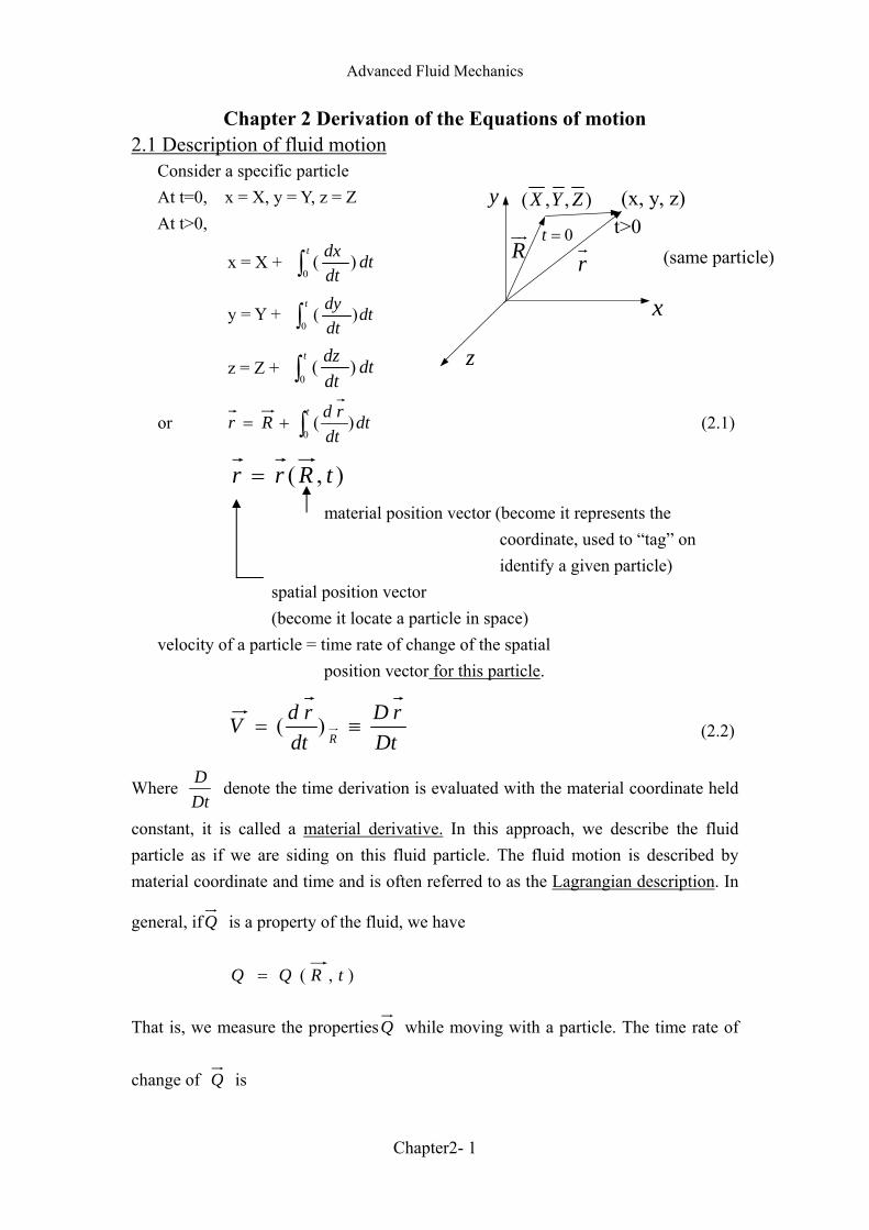
Chapter 2 Derivation of the Equations of motion 2.1 Description of fluid motion
Consider a specific particle At t=0, x = X, y = Y, z = Z At t>0,
x = X + ∫t
dtdtdx
0)(
y = Y + dtdtdyt
∫0)(
z = Z + ∫t
dtdtdz
0)(
or dtdt
rdRrt
)(0∫+= (2.1)
),( tRrr =
material position vector (become it represents the coordinate, used to tag on identify a given particle)
spatial position vector (become it locate a particle in space)
velocity of a particle = time rate of change of the spatial position vector for this particle.
DtrD
dtrdV
R≡= )( (2.2)
Where DtD denote the time derivation is evaluated with the material coordinate held
constant, it is called a material derivative. In this approach, we describe the fluid particle as if we are siding on this fluid particle. The fluid motion is described by material coordinate and time and is often referred to as the Lagrangian description. In
general, ifQ is a property of the fluid, we have
),( tRQQ =
That is, we measure the propertiesQ while moving with a particle. The time rate of
change of Q is

Advanced Fluid Mechanics
Chapter2- 2
(x, y, z)y
x
z
=kdt
dQ )( ( ) ( )lim[ ]Rt
Q t t Q t DQt Dt→∞
+ −="!
#
##
Note that ( )Q t t+# and Q(t) us the properties of Q for the same fluid particle. However, Q may be measured at a point fixed in space by a instrument. That is
( , , , ) ( , )Q Q x y z t Q r t= =!
(2.3)
This is called a 〝Euler Description〞.
If the spatial coordinate r!
are held constant while we take the limit ( ) ( )( ) lim[ ]r rt
dQ Q dy Q t t Q tdt t dx t→∞
∂ + −= =∂
! !#
##
The relation between ( ) r
dQdt
! and ( )R
dQdt
"! is as follows:
( , ) ( ( , ), )Q Q r t Q r R t t= =! ! "!
[ ( , ), ( , ), ( , ), ]Q x R t y R t z R t t="! "! "!
( ) ( )( ) ( )( ) ( )( )R R R R
dQ DQ Q dx Q dy Q dz Qdt Dt x dt y dt z dt t
∂ ∂ ∂ ∂= = + + +
∂ ∂ ∂ ∂"! "! "! "!
u v w = ( )r
dQdt
!
∴ ( ) ( ) QR r
d Q d Q Vd t d t
= +"! !"!i∇ (2.4a)
or
DQ Q VDt t
∂= +∂
"!i Q∇ (2.4b)
(Convective derivative) (Unsteady derivative or local derivative)
(Material Derivative substantial Euler derivative) If moves with the same does stay in a stationary location, nor moves with same
velocity as the fluid particle ( )V"!
, but moves with velocity bV""!
, then
( , )Q Q r t=!
dQ Q Q dx Q dy Q dzdt t X dt y dt z dt
∂ ∂ ∂ ∂= + + +∂ ∂ ∂ ∂

Advanced Fluid Mechanics
Chapter2- 3
( )r t t+!#
( )r t!
• •( , )V r t"! !
bV"!
( , )V r r t t+ +"! ! !
# #
Inertia coordinate system
and
DQ Q Vdt t
∂= +∂
"!i Q∇ (2.5)
( )rdQ Qdt t
∂=∂
"!
( )observerdQdt = The time rate of change of fluid property ( , )Q r t
!measured by
the observer.
= ( )bQ V Vt
∂+ −
∂
"! ""!i Q∇
Similarly:
a!
= acceleration of a fluid particle = time rate of change of the fluid particle
= ( )R
dV DV V Vdt Dt t
∂= = +
∂"!
"! "! "! "! "!i V∇ (2.6)
Note: (1) Observer riding with the fluid particle would describe his acceleration in
terms of a single vector a!
; the fixed observer would note theV"!
, V"!
,
Vt
∂∂
"!, and from these quantities be would deduce the acceleration.
(2) If the flow is steady ( 0)Vt
∂=
∂
"!, the acceleration is not necessarily zero.
Since, from (2.6)
Va V= ⋅! "! "!
∇
Advanced Fluid Mechanics
Chapter2- 4
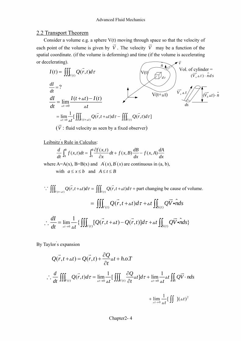
2.2 Transport Theorem Consider a volume e.g. a sphere V(t) moving through space so that the velocity of each point of the volume is given by V
"!. The velocity V
"! may be a function of the
spatial coordinate. (if the volume is deforming) and time (if the volume is accelerating or decelerating).
( )( ) ( , )
V tI t Q r t dτ= ∫∫∫
!
dIdt=?
0
( ) ( )limt
dI I t t I tdt t→
+ −=#
##
( ) ( )0
1lim [ ( , ) ( , ) ]V V tt t t
Q r t t d Q r t dt
τ τ→ +
= + −∫∫∫ ∫∫∫# #
! !#
#
(V"!
: fluid velocity as seen by a fixed observer)
Leibnitzs Rule in Calculus:
( , )( , ) ( , ) ( , )B B
A A
d f x t dB dAf x t dt dt f x B f x Adt x dx dx
∂= + −
∂∫ ∫
where A=A(x), B=B(x) and ' '( ), ( )A x B x are continuous in (a, b), with a x b≤ ≤ and A t B≤ ≤
∵( ) ( )
( , ) ( , )V t t V t
Q r t t d Q r t t dτ τ+
+ = + +∫∫∫ ∫∫∫#
! !# # part changing be cause of volume.
%( ) ( )
( , )V t S t
Q r t t d t QV ndsτ= + +∫∫∫ ∫∫! "!# # i
∴%
0 ( ) ( )lim
1 [ ( , ) ( , )] t V t S t
dI Q r t t Q r t d t QV ndsdt t
τ→
= + − +∫∫∫ ∫∫#
! ! "!# # i
#
By Taylors expansion
( , ) ( , ) . .QQ r t t Q r t t h oTt
∂+ = + +
∂
! !# #
∴( ) ( )0 0
1 1( , ) lim [ ] limV t V t St t
d QQ r t d t d t QV ndsdt t t t
τ τ→ →
∂= + ⋅
∂∫∫∫ ∫∫∫ ∫∫# #
! "!# #
# #
2
0
1lim [ ]( )t
tt→
+ ∫∫##
#
V"!
%n
dτ%( )sV t nd s⋅
""!#
sV t""!#
ds
%( )SV t n⋅""!#
Vol. of cylinder =V(t)
V(t+ t)#
Advanced Fluid Mechanics
Chapter2- 5
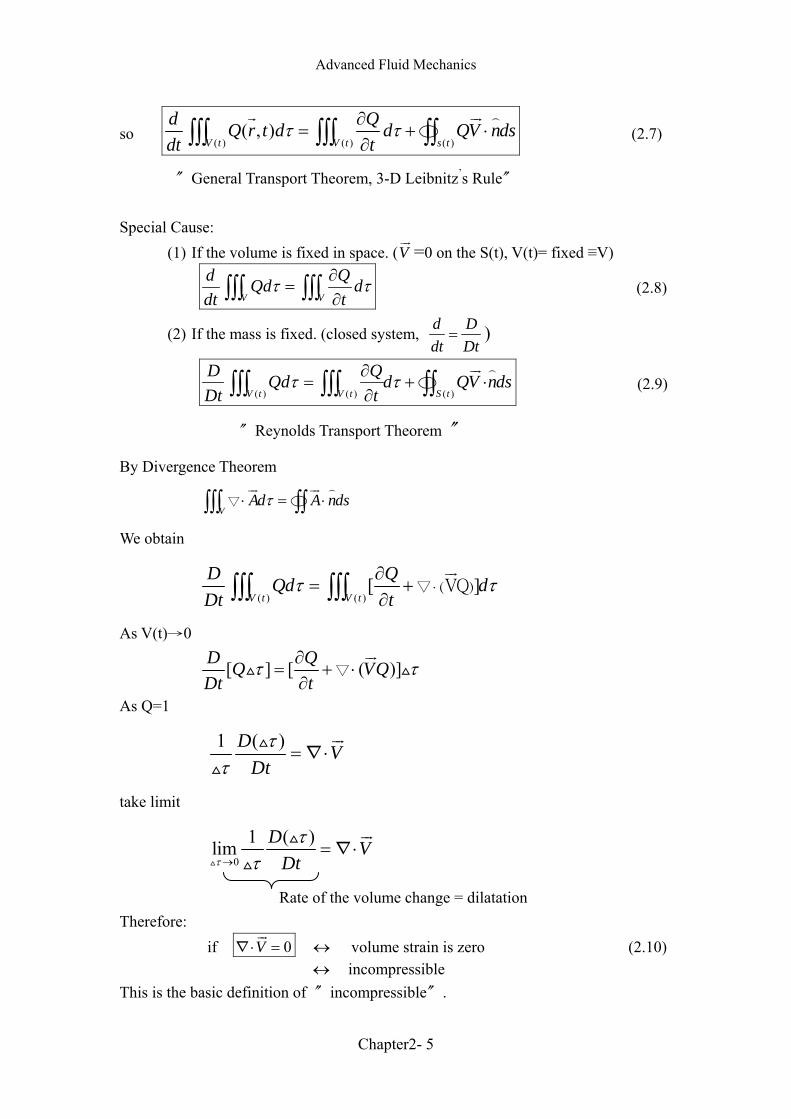
so ( ) ( ) ( )
( , )V t V t s t
d QQ r t d d QV ndsdt t
τ τ∂= + ⋅
∂∫∫∫ ∫∫∫ ∫∫! "! &
' (2.7)
〞General Transport Theorem, 3-D Leibnitzs Rule〞 Special Cause:
(1) If the volume is fixed in space. (V"!
=0 on the S(t), V(t)= fixed ≡V)
V V
d QQd ddt t
τ τ∂=
∂∫∫∫ ∫∫∫ (2.8)
(2) If the mass is fixed. (closed system, d Ddt Dt= )
( ) ( ) ( )V t V t S t
D QQd d QV ndsDt t
τ τ∂= + ⋅
∂∫∫∫ ∫∫∫ ∫∫"! &
' (2.9)
〞Reynolds Transport Theorem 〞
By Divergence Theorem
VAd A ndsτ⋅ = ⋅∫∫∫ ∫∫"! "! &'
We obtain
( ) ( )[ ]
V t V t
D QQd dDt t
τ τ⋅∂
= +∂∫∫∫ ∫∫∫
"! ( )VQ
As V(t)→0
[ ] [ ( )]D QQ VQDt t
τ τ∂= + ⋅
∂
"!# #
As Q=1
1 ( )D VDtτ
τ= ⋅
"!##
∇
take limit
0
1 ( )lim D VDtτ
ττ→
= ⋅#
"!##
∇
Rate of the volume change = dilatation Therefore:
if 0V⋅ ="!
∇ ↔ volume strain is zero (2.10) ↔ incompressible
This is the basic definition of 〞incompressible〞.
Advanced Fluid Mechanics
Chapter2- 6
.C VV"!
V"!
t
t+ t#
Control volume velocity
(Fluid particle velocity)
Control volume and system at time t
:control volume at t+ t#
:System at t+ t#
V"!
.C VV"!
.C VVr V V= −"! "! "!
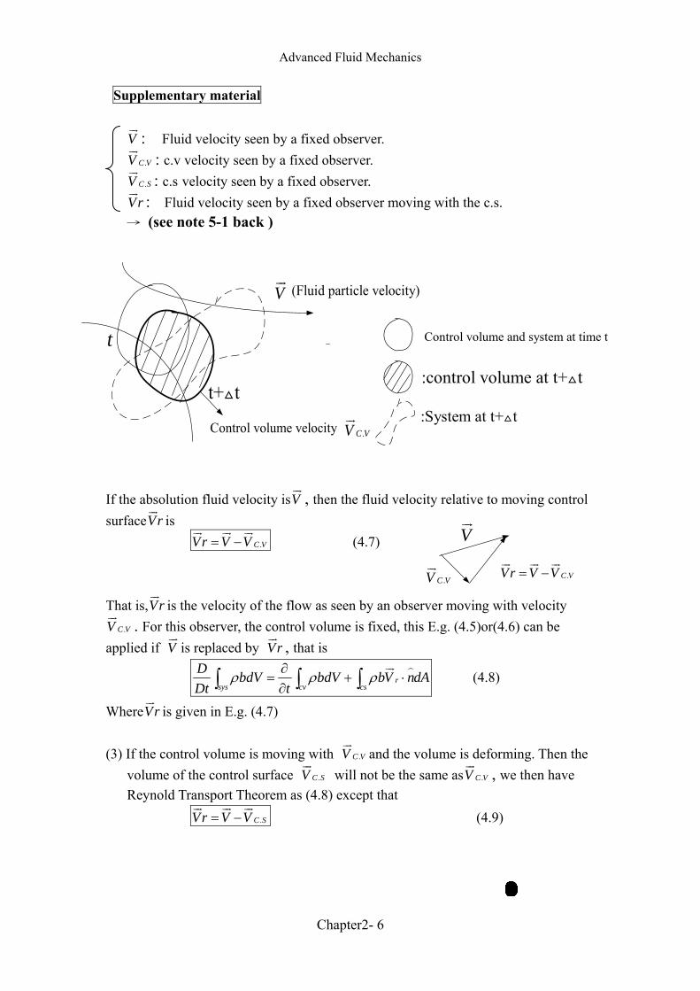
Supplementary material
V"!
: Fluid velocity seen by a fixed observer. .C VV
"!: c.v velocity seen by a fixed observer.
.C SV"!
: c.s velocity seen by a fixed observer. Vr"!
: Fluid velocity seen by a fixed observer moving with the c.s. → (see note 5-1 back ) If the absolution fluid velocity isV
"!, then the fluid velocity relative to moving control
surfaceVr"!
is .C VVr V V= −
"! "! "! (4.7)
That is,Vr
"!is the velocity of the flow as seen by an observer moving with velocity
.C VV"!
. For this observer, the control volume is fixed, this E.g. (4.5)or(4.6) can be applied if V
"!is replaced by Vr
"!, that is
rsys cv cs
D bdV bdV bV ndADt t
ρ ρ ρ∂= + ⋅∂∫ ∫ ∫
"! & (4.8)
WhereVr"!
is given in E.g. (4.7) (3) If the control volume is moving with .C VV
"!and the volume is deforming. Then the
volume of the control surface .C SV"!
will not be the same as .C VV"!
, we then have Reynold Transport Theorem as (4.8) except that
.C SVr V V= −"! "! "!
(4.9)
Advanced Fluid Mechanics
Chapter2- 7
V"!
n
2.3 Conservation of Mass
(1) For a closed system: ( 0m⋅
= , Lagrangian Description )
( )0
V t
D dDt
ρ τ =∫∫∫
( ) ( )V t s td V nds
tρ τ ρ∂
= + ⋅∂∫∫∫ ∫∫
"! &'
( )[ ]
V td
tρ
ρ τ⋅=∂ +∂∫∫∫
""! ( )V
if V(t) is arbitrary and the integrand is continuous, then
( ) 0Vtρ ρ∂+ ⋅ =
∂
"!∇ 〞Continuity equation〞 (2.11)
(Since it is continuous in the 1st order) or
0V Vtρ ρ ρ∂+ ⋅ + ⋅ =
∂
""! "!∇ ∇
( )R
d Ddt Dtρ ρ
= ="!
⇒ 0D VD tρ ρ+ ⋅ =
"!∇ (2.12)
Special Cases:
(a) For a steady flow: ( 0t∂=
∂)
⇒ ( ) 0Vρ⋅ ="!
(b) For a incompressible flow: ( 0V⋅ ="!
∇ )
E.g. (2.12)⇒ 0DDtρ=
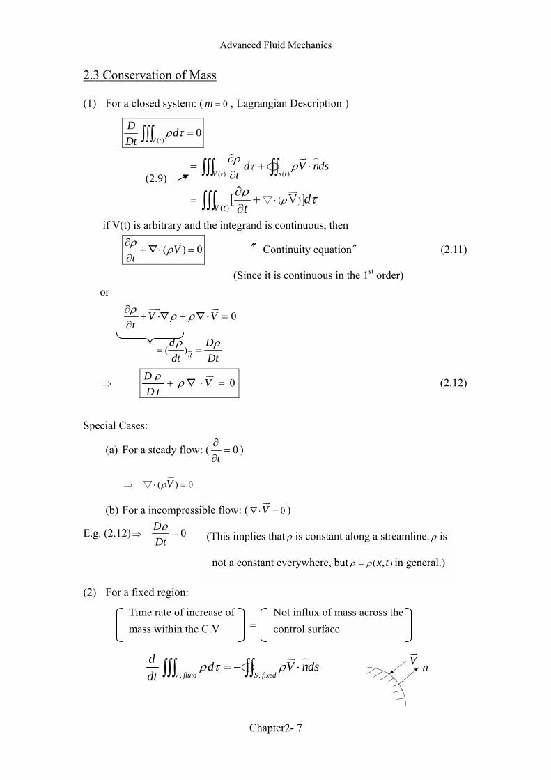
(2) For a fixed region: =
. .V fluid S fixed
d d V ndsdt
ρ τ ρ= − ⋅∫∫∫ ∫∫"! &
'
(2.9)
(This implies that ρ is constant along a streamline. ρ is
not a constant everywhere, but ( ),x tρ ρ=!
in general.)
Time rate of increase of mass within the C.V
Not influx of mass across the control surface
Advanced Fluid Mechanics
Chapter2- 8
Since V, S is fixed, from E.g. (2.8) with Q= ρ , we have
V V
d d ddt t
ρρ τ τ∂=
∂∫∫∫ ∫∫∫
Therefore
V Sd V ndsρ τ ρ= − ⋅∫∫∫ ∫∫
"! &' 〞conservation of mass〞 (2.13)
fixed fixed
Advanced Fluid Mechanics
Chapter2- 9
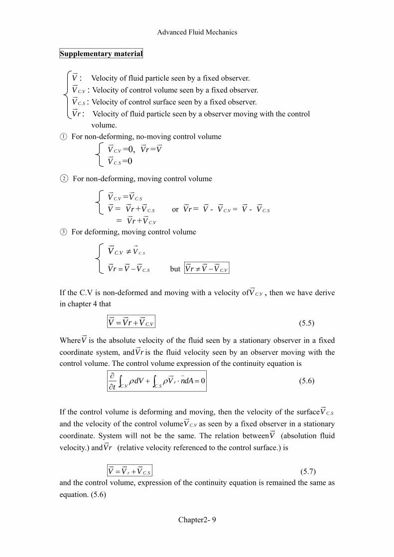
Supplementary material
V"!
: Velocity of fluid particle seen by a fixed observer. .C VV
"!: Velocity of control volume seen by a fixed observer.
.C SV"!
: Velocity of control surface seen by a fixed observer. Vr"!
: Velocity of fluid particle seen by a observer moving with the control volume.
1 For non-deforming, no-moving control volume
.C VV"!
=0, Vr"!
=V"!
.C SV
"!=0
2 For non-deforming, moving control volume
.C VV"!
= .C SV"!
V"!
= Vr"!
+ .C SV"!
or Vr"!
= V"!
- .C VV"!
= V"!
- .C SV"!
= Vr"!
+ .C VV"!
3 For deforming, moving control volume
.. C SC V VV ≠"! !
.C SVr V V= −"! "! "!
but .C VVr V V≠ −"! "! "!
If the C.V is non-deformed and moving with a velocity of .C VV"!
, then we have derive in chapter 4 that
.C VV Vr V= +"! "! "!
(5.5)
WhereV"!
is the absolute velocity of the fluid seen by a stationary observer in a fixed coordinate system, andVr
"!is the fluid velocity seen by an observer moving with the
control volume. The control volume expression of the continuity equation is
. .0r
C V C SdV V ndA
tρ ρ∂
+ ⋅ =∂ ∫ ∫
"! & (5.6)
If the control volume is deforming and moving, then the velocity of the surface .C SV
"!
and the velocity of the control volume .C VV"!
as seen by a fixed observer in a stationary coordinate. System will not be the same. The relation betweenV
"! (absolution fluid
velocity.) andVr"!
(relative velocity referenced to the control surface.) is
.r C SV V V= +"! "! "!
(5.7) and the control volume, expression of the continuity equation is remained the same as equation. (5.6)
Advanced Fluid Mechanics
Chapter2- 10
2.4 Equation of Change for momentum Newtons second low
dVF ma mdt
= ="!"! !
applies only for a point particle of fixed mass m. For a closed system (Lagrangian description), it become
( )V t
D Vd FDt
ρ τ =∑∫∫∫"! "!
(2.14)
The external not forces include forces acting on the body (volume) and on the surface, namely.
body surfaceF F F= +∑"! "! "!
Neglecting magnetic & electrical effect, the only body force is due to the gravitational force, thus
( )body
V tF f dρ τ= ∫∫∫"! "!
Where f"!
represent the body force per unit mass.
For any arbitrary position, the surface stresses (surface force/area) not only depend on the direction of the force, but also on the orientation of the surface. Therefore, the surface stress is a second order tension, and is denoted byσ
(!.
Before we involve on the derivation of surfaceF"!
, we need to know more about
tension. 〞pressure〞means the normal force per unit area acted on the fluid particle> As the fluid is static, the pressure of the fluid is called hydrostatic pressure. Since
the fluid is motionless, the fluid is in equilibrium, therefore the (Hydrostatic pressure = thermodynamic pressure)
As the fluid is in motion, the 3 principal normal stresses are not necessary equal, and the fluid is not in equilibrium. Therefore, the hydrodynamic pressure is defined by
(Hydrostatic pressure) ≡ 1 ( )3 xx yy zzσ σ σ+ +
and which is not equal to the thermodynamic pressure either. Later we will prove that
(Hydrostatic pressure) = thermodynamic pressure + '13λ
= (Hydrostatic pressure)

Advanced Fluid Mechanics
Chapter2- 11
Supplementary material 5.2 Conservation of momentum Consider a particular moment when the control volume is coincide with the control volume, then
.system C VF F=∑ ∑"! "!
(5.7)
Newtons 2nd law for the control mass system is
syssys
D VdV FDt
ρ =∑∫"! "!
(5.8)
From Reynolds Transport Theorem for a fixed spaced, non-deforming control volume.
. .sys C V C S
D VdV V dV V V ndADt t
ρ ρ ρ∂= + ⋅∂∫ ∫ ∫
"! "! "! "! &
Apply (5.7) & (5.8) into above equation, we can get the momentum equation for a control volume.
.. .
C VC V C S
V dV V V ndA Ft
ρ ρ∂+ ⋅ =
∂ ∑∫ ∫"! "! "! "!&
(5.9)
Remark:
If the control volume is non-deforming, but moves with a velocity of .C VV"!
, then we may take b= V
"! in equation (4.8), and get
. .r
sys C V C S
D V dV V dV V V ndADt t
ρ ρ ρ∂= + ⋅∂∫ ∫ ∫
"! "! "! "! &
Combined with (5.7) & (5.8), the above equation can be written as
.. .
C VrC V C S
V dV V V ndA Ft
ρ ρ∂+ ⋅ =
∂ ∑∫ ∫"! "! "! "!&
(5.10)
= Sum of external forces acting on the system
= time rate of change of the linear momentum of the system
= time rate of change of the linear momentum of the system
= not rate of flow of linear momentum through the C.S.

Advanced Fluid Mechanics
Chapter2- 12
Since .C VV Vr V= +"! "! "!
Equation (5.10) ⇒
.. .. .
( ) ( ) C Vr C V r C V rC V C S
V V dV V V V ndA Ft
ρ ρ∂+ + + ⋅ =
∂ ∑∫ ∫"! "! "! "! "! "!&
(5.11)
(Non-deforming + moving C.V) If the flow is steady, then
..
( ) 0r C VC V
V V dVt
ρ∂+ =
∂ ∫"! "!
and from the continuity equation
. .0r
C V C SdV V ndA
tρ ρ∂
+ ⋅ =∂ ∫ ∫
"! & (*)
The momentum equation of (5.11) reduces to
... .
C Vr r C V rC S C S
V V ndA V V ndA Fρ ρ⋅ + ⋅ =∑∫ ∫"! "! "! "! "!& &
..
0C V rC S
V V ndAρ= ⋅ =∫"! "! &
from equation(*)
or
..
C Vr rC S
V V ndA Fρ ⋅ =∑∫"! "! "!&
(5.12)
(For a non-deforming C.V moving with a constant velocity in a steady state flow)
Advanced Fluid Mechanics
Chapter2- 13
Aside: A second order tension, called a dyad and denoted as AB"!"!
, satisfies the following properties:
( ) ( )AB C A B C⋅ = ⋅"!"! "! "! "! "!
( ) ( )C AB C A B⋅ = ⋅"! "!"! "! "! "!
A unit tension, II("!
, is a tension with C C⋅ =
(! "! "!Ⅱ , C C⋅ =
"! (! "!Ⅱ
In a Cartesian coordinate system,
ii j j kk= + +(! !! !! ! !Ⅱ
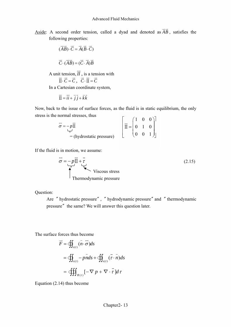
Now, back to the issue of surface forces, as the fluid is in static equilibrium, the only stress is the normal stresses, thus
pσ = −(! (!
Ⅱ
= (hydrostatic pressure) If the fluid is in motion, we assume:
pσ τ= − +(! (! )
Ⅱ (2.15)
Viscous stress Thermodynamic pressure Question:
Are 〞hydrostatic pressure〞, 〞hydrodynamic pressure〞and 〞thermodynamic pressure〞the same? We will answer this question later.
The surface forces thus become
( )( )
s tF n dsσ= ⋅∫∫"! (!&'
( ) ( )( )
s t s tpnds n dsτ= − + ⋅∫∫ ∫∫
)& &' '
( )[ ]
R tp dτ τ= − + ⋅∫∫∫
)* ∇ ∇
Equation (2.14) thus become
1 0 00 1 00 0 1
=
(!Ⅱ

Advanced Fluid Mechanics
Chapter2- 14
momentum flux tensor
( ) ( ) ( )[ ]
R t R t R t
D Vd f d p dDt
ρ τ ρ τ τ τ= + − + ⋅∫∫∫ ∫∫∫ ∫∫∫"! "! )
∇ ∇
= ( ) ( )
( ) ( )R t S t
V d V V ndstρ τ ρ∂
+ ⋅∂∫∫∫ ∫∫"! "! "! &
'
= ( )
( )[ ( )]R t
V V V dtρ ρ τ∂
+ ⋅∂∫∫∫"! "! "!
∇
⇒ ( ) ( )V V V f p
tρ ρ ρ τ∂
+ ⋅ = − + ⋅∂
"! "! "! "! )∇ ∇ ∇ (2.16)
or
( ) ( ) ( ) ( )R t R t R t R t
D D DV DVV d V dm dm dDt Dt Dt Dt
ρ τ ρ τ= = =∫∫∫ ∫∫∫ ∫∫∫ ∫∫∫"! "!"! "!
Equation (2.16) thus has another form of
D V f pD t
ρ ρ τ= − + ⋅"! "! )
∇ ∇ (2.17)
Equation (2.17) may be derived from (2.16) either
L.H.S = ( ) ( )V V Vtρ ρ∂
+ ⋅∂
"! "! "!∇
= ( ) ( )( )V V V V V Vt t
ρρ ρ ρ∂ ∂
+ + ⋅ + ⋅∂ ∂
"! "! "! "! "! "!∇ ∇
= ( )V V V V Vt t
ρρ ρ
∂ ∂ + ⋅ + + ⋅ ∂ ∂
"! "! "! "! "!∇ ∇
= DVDt
ρ
"!
By the tenor operation, we show that the left-hand side of the equation (2.16) & (2.17) are identical.
∵DDt
means we follow a fluid particle,
thus the mass dm is a constant, and not a function of time & location.
(= 0 from continuity equation)
(2.9)
(2.16)
Advanced Fluid Mechanics
3- 1
Chapter 3 Exact Solution of N-S Equation Assumptions: 1 Constant Density (Incompressible Flow)
2 Constant µ, k, vC , pC ve C T=
3 No body forces 3.1 Parallel Flow
V u i v j w k= + +
=0 =0 or
0v w= = , but
( , , , )u u x y z t= , ( , , , )p p x y z t= , ( , , , )T T x y z t=
1) Continuity equation: 0 0
0V⋅ =∇ ⇒ 0u v wx y z∂ ∂ ∂
+ + =∂ ∂ ∂
⇒ 0ux∂
=∂
⇒ u does not depend on x
or ( , , )u u y z t= 2) Momentum equation:
V V Vt
ρ µ∂ + ⋅ = − ∂ V 2∇ ∇P+ ∇
or
2 2 2
2 2 2
u u u u p u u uu v wt x y z x x y z
ρ µ ∂ ∂ ∂ ∂ ∂ ∂ ∂ ∂
+ + + = − + + + ∂ ∂ ∂ ∂ ∂ ∂ ∂ ∂
2 2 2
2 2 2
v v v v p v v vu v wt x y z y x y z
ρ µ ∂ ∂ ∂ ∂ ∂ ∂ ∂ ∂
+ + + = − + + + ∂ ∂ ∂ ∂ ∂ ∂ ∂ ∂
2 2 2
2 2 2
w w w w p w w wu v wt x y z z x y z
ρ µ ∂ ∂ ∂ ∂ ∂ ∂ ∂ ∂
+ + + = − + + + ∂ ∂ ∂ ∂ ∂ ∂ ∂ ∂
⇒ 0p py z∂ ∂
= =∂ ∂
⇒ ( , )p p x t=
Advanced Fluid Mechanics
3- 2
2 2
2 2
u p u ut x y z
ρ µ ∂ ∂ ∂ ∂
= − + + ∂ ∂ ∂ ∂ (3.1)
if we 2 2
2 2
u p u ux t x y z
ρ µ ∂ ∂ ∂ ∂ ∂
= − + + ∂ ∂ ∂ ∂ ∂
⇒ 2 2
2 2( ) ( ) ( ) ( )u p u ut x x x y x z x
ρ µ ∂ ∂ ∂ ∂ ∂ ∂ ∂ ∂
= − + + ∂ ∂ ∂ ∂ ∂ ∂ ∂ ∂
⇒ 2
2 0px
∂=
∂ or p
x∂
=∂
function of t only.
∴ ( , , )u u t y z= , ( , )p p x t= , ( )np fx
t∂=
∂
3) Energy equation: Eq. (2.40) ⇒ (v=0) (w=0)
2 2 22 ( ) ( ) ( )vT T T T u v wC u v wt x y z x y z
ρ µ ∂ ∂ ∂ ∂ ∂ ∂ ∂
+ + + = + + ∂ ∂ ∂ ∂ ∂ ∂ ∂
2 2 22 2 2
2 2 2
1 ( ) ( ) ( ) ( )2
u v u w v w T T Tky x z x z y x y z
∂ ∂ ∂ ∂ ∂ ∂ ∂ ∂ ∂+ + + + + + + + + ∂ ∂ ∂ ∂ ∂ ∂ ∂ ∂ ∂
⇒2 2 2
2 22 2 2( ) ( ) ( )v
T T u u T T TC u kt x y z x y z
ρ µ ∂ ∂ ∂ ∂ ∂ ∂ ∂
+ = + + + + ∂ ∂ ∂ ∂ ∂ ∂ ∂ (3.2)
∴ ( , , , )T T t x y z= 3.1.1 Steady, Parallel, 2-D Flow
( 0 , 0 )t z∂ ∂
= =∂ ∂
From the pressure discussion, we know
( )u u y= , ( )p p x= , ( , )T T x y= , constantp dpx dx∂
= =∂
The Equation of motion become 2
2 constantu dpy dx
µ ∂= =
∂ (3.3a)
2 22
2 2( )vT u T TC u kx y x y
ρ µ ∂ ∂ ∂ ∂
= + + ∂ ∂ ∂ ∂ (3.3b)
0 0 0
Advanced Fluid Mechanics
3- 3
integrate Eq (3.3a), we have 2
1 2( ) ( )2y dpu y C y C
dxµ= + + (3.4)
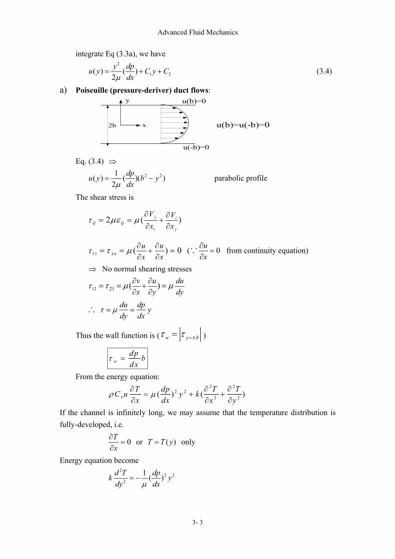
a) Poiseuille (pressure-deriver) duct flows:
2b x
y u(b)=0
u(-b)=0
u(b)=u(-b)=0
Eq. (3.4) ⇒
2 21( ) ( )( )2
dpu y b ydxµ
= − parabolic profile
The shear stress is
2 ( )j i
i jij ij
V Vx x
τ µε µ∂ ∂
+∂ ∂
= =
11 ( ) 0xxu ux x
τ τ µ ∂ ∂+
∂ ∂= = = (∵ 0u
x∂
=∂
from continuity equation)
⇒ No normal shearing stresses
12 21 ( )v u dux y dy
τ τ µ µ∂ ∂+
∂ ∂= = =
∴ du dp ydy dx
τ µ= =
Thus the wall function is ( w y bτ τ =±= )
wd p bd x
τ =
From the energy equation: 2 2
2 22 2( ) ( )v
T dp T TC u y kx dx x y
ρ µ∂ ∂ ∂= + +
∂ ∂ ∂
If the channel is infinitely long, we may assume that the temperature distribution is fully-developed, i.e.
0Tx
∂=
∂ or ( )T T y= only
Energy equation become 2
2 22
1 ( )d T dpk ydy dxµ
= −

Advanced Fluid Mechanics
3- 4
integrate twice 4
23 4
1( ) ( )12
dp yT y C y Ck dxµ
= − + +
If the B.C’S are: ( ) wT b T += , ( ) wT b T −− = , then
4 42
4( ) ( ) (1 )2 2 12
w w w wT T T T y b dp yT yb k dx bµ
+ − + −+ += + + −
When we calculate u(y), we are actually interested in the value of wτ . Similarly, as we solve the temperature distribution, we want to know the heat transfer on the walls. Aside:
In the temperature section, we mentioned that
( ) fluid solid fluidTk qn →
∂=
∂
For the current case
n ( )q q n qn= − = −
q qn= −
On upper surface
On lower surface
q
therefore q k T= − ∇
n n
fluid
Tqe k en
∂− = − ⇒
∂ s F
fluid
Tq kn→
∂=
∂
However, this is not a good way become ne always change its direction for a fixed coordinate frame. Therefore, we may take the positive valve of q as heat transfer in the direction of the positive-coordinate axis, then
q k p= − ∇
⇒ ( )x y zT T Tq i q j q k k i j kx y z
∂ ∂ ∂+ + = − + +
∂ ∂ ∂
⇒ xTq kx
∂= −
∂, y
Tq ky
∂= −
∂, z
Tq kz
∂= −
∂

Advanced Fluid Mechanics
3- 5
At any point, if 0xq > , it means the x-component of the heat transfer at this point is in the +x-axis direction.
For this case:
qy
x
1
2
Therefore, we set q in the direction of +y, then
dTq kdy
= −
(i) If a t p o in t0q >
①, it means q is transferred upward, therefore, it is from
the lower wall to the fluid.
(ii) If a t p o in t0q <
①, the heat is transferred downward, therefore, it is from
the fluid to the lower wall.
(iii)If a t p o in t0q >
②⇒ fluid to upper wall.
(iv) If a t p o in t 0q <②
⇒ upper wall to the fluid #
Take
q q j=
y
x
then dTq k
dy= −
or 3
2 31 ( ) ( )2 3
w wT T b dp yq kb k dx bµ
+ − += − −
Hence
321( ) ( )
2 3w wT T b dpq b k q
b k dxµ
+ −+ −
= − − ≡
321( ) ( )
2 3w wT T b dpq b k q
b k dxµ
+ −− −
− = − − ≡
q>0, heat transfer upward q<0, heat transfer downward
Advanced Fluid Mechanics
3- 6
Remark:
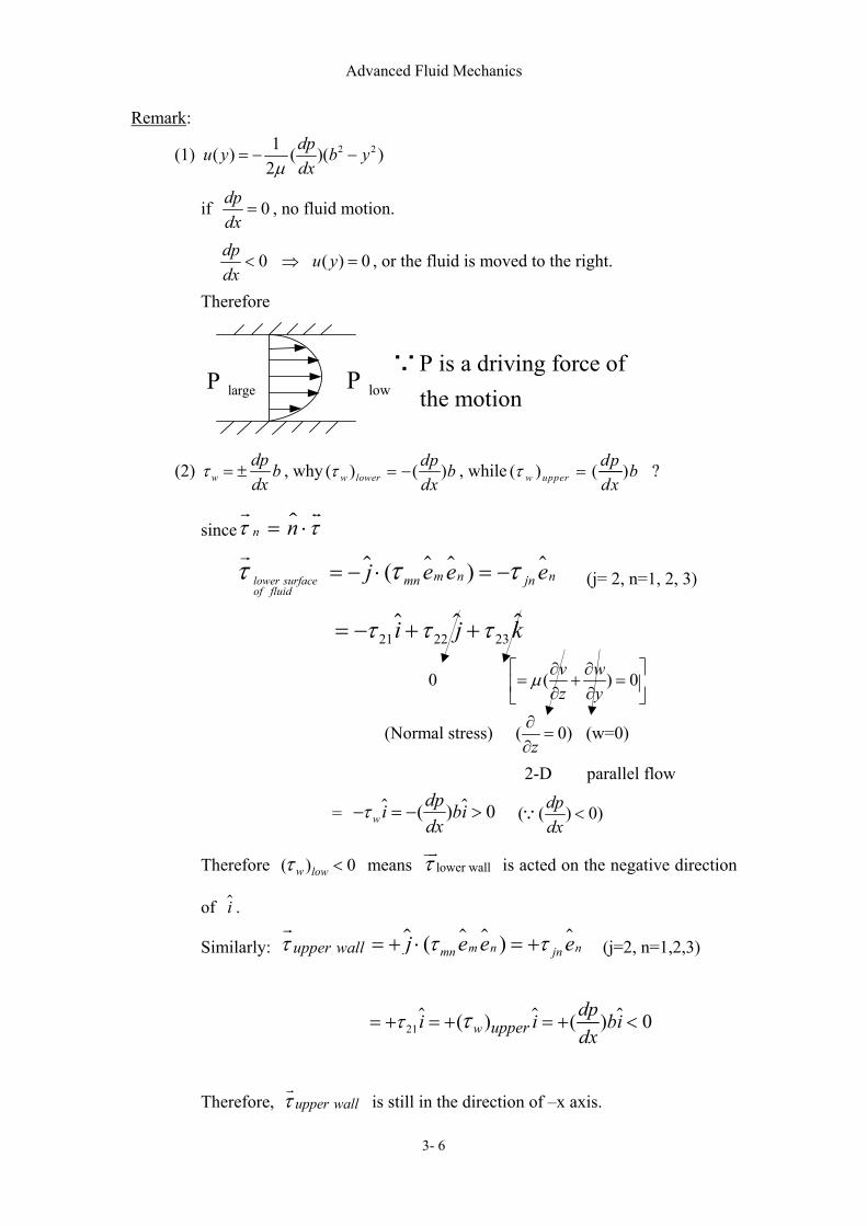
(1) 2 21( ) ( )( )2
dpu y b ydxµ
= − −
if 0dpdx
= , no fluid motion.
0dpdx
< ⇒ ( ) 0u y = , or the fluid is moved to the right.
Therefore
P is a driving force of the motion∵
lowP largeP
(2) wdp bdx
τ = ± , why ( ) ( )w lowerdp bdx
τ = − , while ( ) ( )w upperdp bdx
τ = ?
since n nτ τ= ⋅
( )lower surfaceof fluid
m n nmn jnj e e eτ τ τ= − ⋅ = −
(j= 2, n=1, 2, 3)
21 22 23i j kτ τ τ= − + +
0 ( ) 0v wz y
µ ∂ ∂= + = ∂ ∂
(Normal stress) ( 0)z∂=
∂ (w=0)
2-D parallel flow
= ( ) 0wdpi bidx
τ− = − > ( ( ) 0)dpdx
<∵
Therefore ( ) 0w lowτ < means lower wallτ is acted on the negative direction
of i .
Similarly: ( )m n nmn jnupper wall j e e eτ τ τ= + ⋅ = + (j=2, n=1,2,3)
21 ( ) ( ) 0w upperdpi i bidx
τ τ= + = + = + <
Therefore, upper wallτ is still in the direction of –x axis.

Advanced Fluid Mechanics
3- 7
(3) ( ) ( )q b q b≠ − because w wT T+ −≠
However, if w wT T+ −= , we know the results that
32( )
3b dpq
dxµ+ = +
32( )
3b dpq
dxµ− = −
Why these is a difference in sign? Does it mean that one wall is received heat while the other given away the heat? The answer is that
0q+ > ⇒ heat transfer upward ⇒ from fluid to the upper wall 0q− < ⇒ heat transfer downward ⇒ from fluid to the lower wall
To understand the flow in more detail, let’s see the temperature profile for the case of:
w w wT T T+ −= =
4 42
4( ) ( ) (1 )12w
b dp yT y Tk dx bµ
= + −
0≥
wT
wT
wτ
wτ 0
The shearing stress is du dp ydy dx
τ µ= =
Advanced Fluid Mechanics
3- 8
Question: Why the temperature is highest but the shearing stress is minimum (zero) along the centerline?
Answer: The high viscous force along the walls will produce a large amount of dissipation energy. In turn, it will increase the internal energy of the fluid near the wall. Partial internal energy transport to the wall due to dissipation
gradient,3
2( )3wb dpq
dxµ
=
, the rest of viscosity. Along the centerline, the
fluid received the diffused energy from upper & lower surface, thus it has the max temperature.
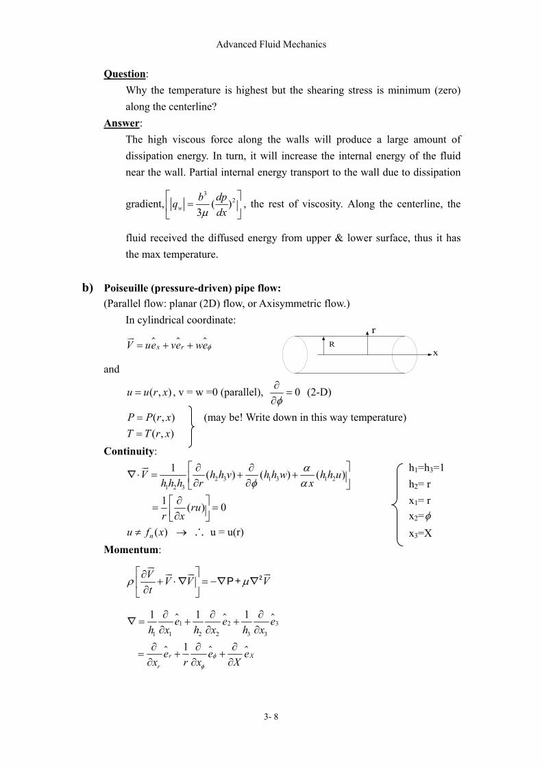
b) Poiseuille (pressure-driven) pipe flow:
(Parallel flow: planar (2D) flow, or Axisymmetric flow.) In cylindrical coordinate:
x rV ue ve weφ= + +
and
( , )u u r x= , v = w =0 (parallel), 0φ∂
=∂
(2-D)
( , )P P r x= (may be! Write down in this way temperature) ( , )T T r x=
Continuity:
2 3 1 3 1 21 2 3
1 ( ) ( ) ( )V h h v h h w h h uh h h r x
αφ α
∂ ∂⋅ = + + ∂ ∂
∇
1 ( ) 0rur x
∂ = = ∂
( )nu f x≠ → ∴ u = u(r) Momentum:
V V V Vt
ρ µ ∂
+ ⋅ = − ∂
2∇ ∇P+ ∇
1 2 3
1 1 2 2 3 3
1 1 1e e eh x h x h x
∂ ∂ ∂= + +
∂ ∂ ∂∇
1r X
r
e e ex r x X
φ
φ
∂ ∂ ∂= + +∂ ∂ ∂
R
r
x
h1=h3=1 h2= r x1= r x2=φ x3=X
Advanced Fluid Mechanics
3- 9
( ) ( ) ( ) ( )x x x r x r xdu duV ue u e u e e e e edr dr
= = + = =∇ ∇ ∇ ∇
0 (∵ xe is fixed, however ,re eφ are not )
( ) ( ) ( )( ) 0x r x x r xdu duV V ue e e u e e edr dr
⋅ = ⋅ = ⋅ =∇
r xp pp e er x∂ ∂
= +∂ ∂
∇
2 3 1 3 1 2
1 2 3 1 1 1 2 2 2 3 3 3
1 ( ) ( ) ( )h h h h h hh h h x h x x h x x h x
∂ ∂ ∂ ∂ ∂ ∂= + + ∂ ∂ ∂ ∂ ∂ ∂
2∇
1 1( ) ( ) ( )r rr r r r x xφ φ ∂ ∂ ∂ ∂ ∂ ∂
= + + ∂ ∂ ∂ ∂ ∂ ∂
2 1 1( ) ( ) ( )V V VV r rr r r r x xφ φ ∂ ∂ ∂ ∂ ∂ ∂
= + + ∂ ∂ ∂ ∂ ∂ ∂ ∇ , ( ) xV u r e=
0 ( ( ) rV u r e= ) 0
1 ( ) xur e
r r r∂ ∂ = ∂ ∂
∴ Momentum equation:
x-dir: 0 ( )p urx r r r
µ∂ ∂ ∂= − +
∂ ∂ ∂ (3.5)
r-dir: 0pr∂
=∂
⇒ p=p(x)
Eq. (3.5) ⇒
( ) constantdp d durdx r dr dr
µ= =
( )nf x ( )nf r
integrate twice with the B.C.’s: (i) u(r) = 0 (ii) 0
0r
dudr =
= , we obtain
2 21( ) ( )4
dpu r R rdxµ
= − − (parabolic profile)
2
max 0
14r
dpu u Rdxµ=
= = −
∵ L.H.S = ( )nf x R.H.S = ( )nf r
∴the only solution is that it is a constant
Advanced Fluid Mechanics
3- 10
Volume flow rate, 4
0( )(2 )
8R R dpQ u r r dr
dxππµ
= = −∫
The mean velocity, 2
2max
8 2uQ R dpu
R dxπ µ= = − =
Shear stress at wall 1 4( )2w
du dp uRdr dx R
µτ µ= = − =
216
1 Re2
wf
D
Cu
τ
ρ≡ = , where D
uDRe ρµ
=
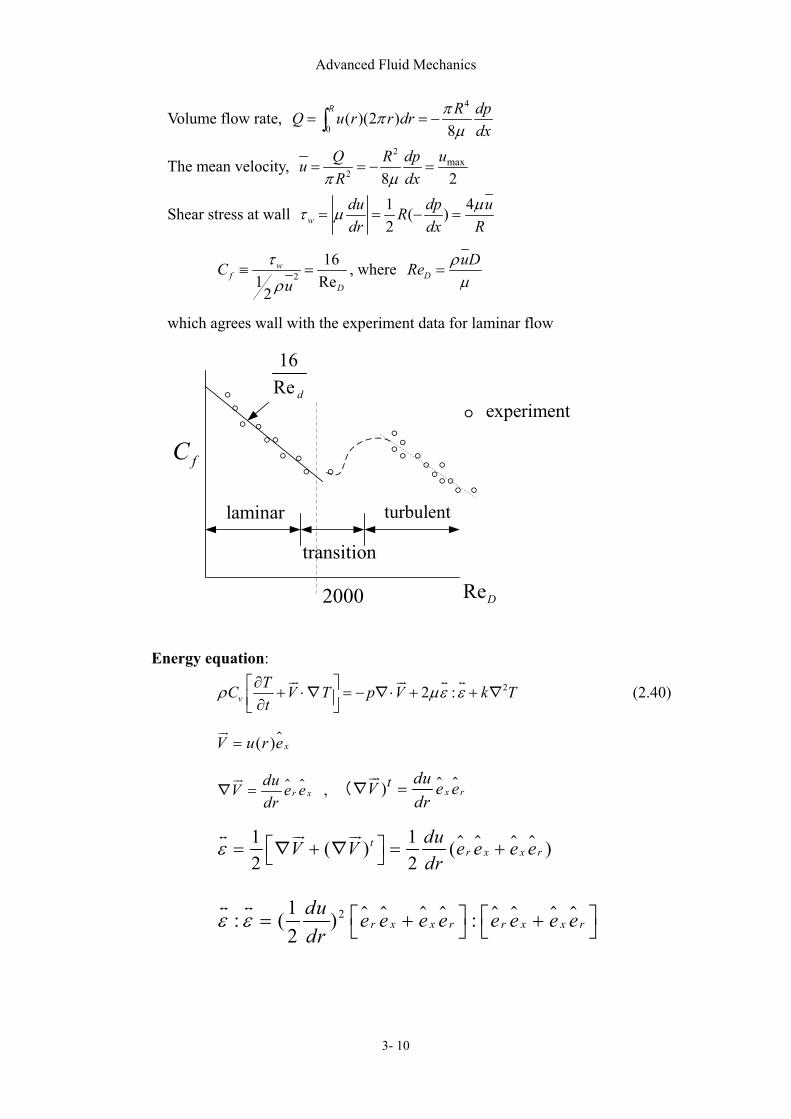
which agrees wall with the experiment data for laminar flow
fC
ReD
16Re d
2000
laminar
transition
turbulent
experiment
Energy equation:
22 :vTC V T p V k Tt
ρ µε ε∂ + ⋅ = − ⋅ + + ∂ ∇ ∇ ∇ (2.40)
( ) xV u r e=
r xduV e edr
=∇ , ) x rt duV e e
dr=(∇
1 1( ) ( )2 2
tr x x r
duV V e e e edr
ε = + = + ∇ ∇
21: ( ) :2
r x x r r x x rdu e e e e e e e edr
ε ε = + +
Advanced Fluid Mechanics
3- 11
21( ) : 2 : :2
r x r x x r r x x r x rdu e e e e e e e e e e e edr
= + +
( )( )1
x x r re e e e= ⋅ ⋅=
( )( )0
r x r xe e e e= ⋅ ⋅=
21 ( )2
dudr
=
0V⋅ =∇ (Incompressible flow)
( ( ) ) ( ..)x xT TV T u r e e ux x
∂ ∂⋅ = ⋅ + =
∂ ∂∇
2 1 1( ) ( ) ( )T T TT r rr r r r x xφ φ ∂ ∂ ∂ ∂ ∂ ∂
= + + ∂ ∂ ∂ ∂ ∂ ∂ ∇
Assume ( )T T r= only then Eq. (2.40) becomes
20 ( ) ( )du k dTrdr r r dr
µ ∂= +
∂ (fully-developed in temperature)
Sub. ( )dudr
into the above equation, and integrate twice with the B.C.’s:
1 ( ) wT r T= 2 0
0r
dTdr =
= , we have
2 4 41( ) ( ) ( )64w
dpT r T R rk dxµ
= + −
Remark:
1 Can discuss 2~ ( )walldpqdx
, while ~ ( )wdpdx
τ and ~ ( )dpQdx
, 4~Q R
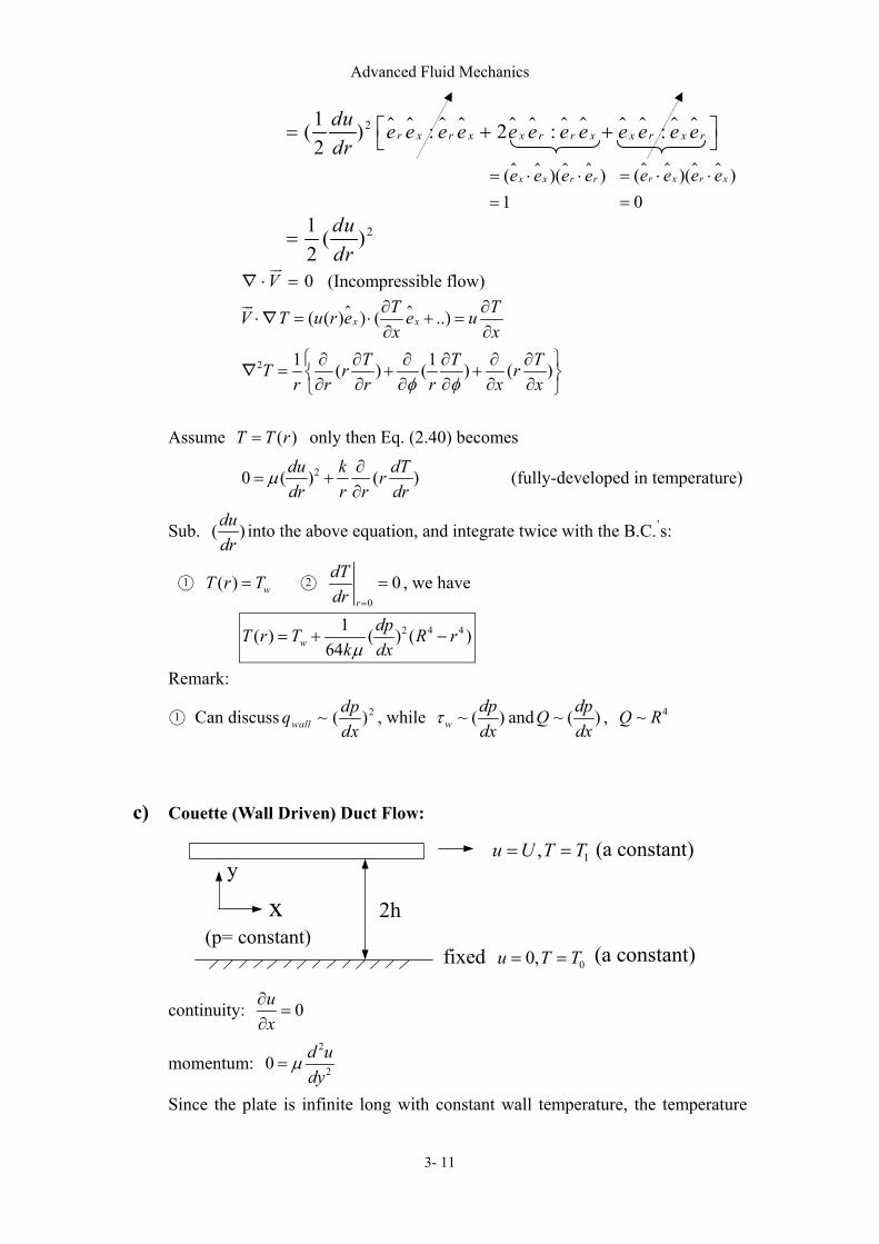
c) Couette (Wall Driven) Duct Flow:
1,u U T T= =
00,u T T= =
xy
(p= constant)
(a constant)
(a constant)
2h
fixed
continuity: 0ux∂
=∂
momentum: 2
20 d udy
µ=
Since the plate is infinite long with constant wall temperature, the temperature
Advanced Fluid Mechanics
3- 12
u(y)U
1.0
0
-1 0
yh
can be assumed fully developed. Thus T=T(y) only. The energy equation reduces to
2
220 ( )du d Tk
dy dyµ= +
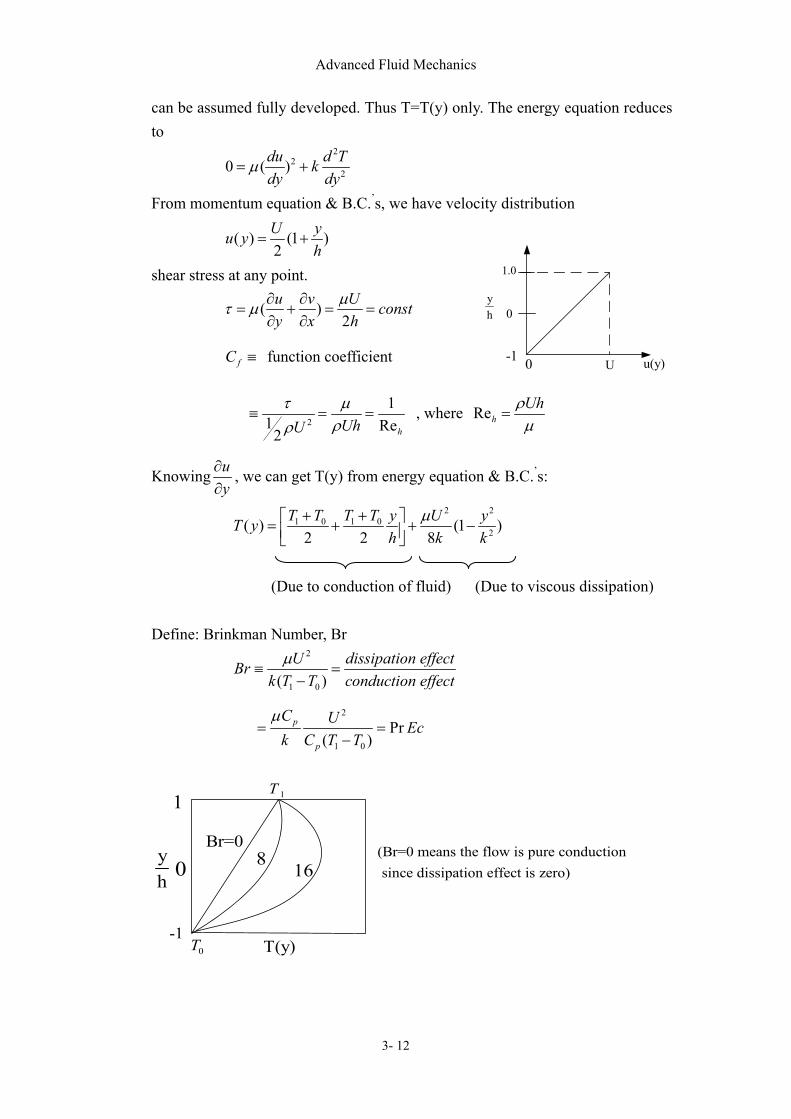
From momentum equation & B.C.’s, we have velocity distribution
( ) (1 )2U yu y
h= +
shear stress at any point.
( )2
u v U consty x h
µτ µ ∂ ∂= + = =
∂ ∂
fC ≡ function coefficient
2
11 Re2 hUhU
τ µρρ
≡ = = , where RehUhρµ
=
Knowing uy∂∂
, we can get T(y) from energy equation & B.C.’s:
2 2
1 0 1 02( ) (1 )
2 2 8T T T T y U yT y
h k kµ+ + = + + −
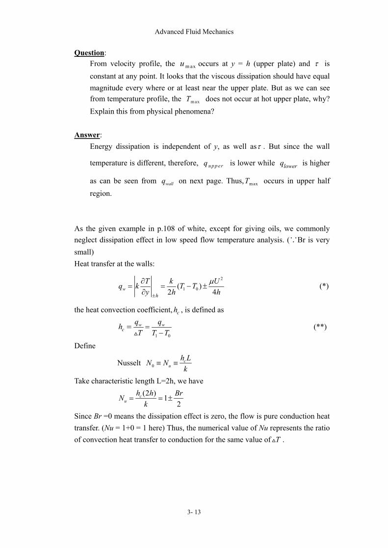
(Due to conduction of fluid) (Due to viscous dissipation)
Define: Brinkman Number, Br
2
1 0( )U dissipation effectBr
k T T conduction effectµ
≡ =−
2
1 0
Pr( )
p
p
C U Eck C T T
µ= =
−
1T
0T
(Br=0 means the flow is pure conduction since dissipation effect is zero)
yh
1
0
-1T(y)
Br=08 16
Advanced Fluid Mechanics
3- 13
Question: From velocity profile, the m axu occurs at y = h (upper plate) and τ is constant at any point. It looks that the viscous dissipation should have equal magnitude every where or at least near the upper plate. But as we can see from temperature profile, the m axT does not occur at hot upper plate, why? Explain this from physical phenomena?
Answer:
Energy dissipation is independent of y, as well asτ . But since the wall
temperature is different, therefore, u p p erq is lower while lowerq is higher
as can be seen from wallq on next page. Thus, maxT occurs in upper half region.
As the given example in p.108 of white, except for giving oils, we commonly neglect dissipation effect in low speed flow temperature analysis. (∵Br is very small) Heat transfer at the walls:
2
1 0( )2 4w
h
T k Uq k T Ty h h
µ
±
∂= = − ±
∂ (*)
the heat convection coefficient, ch , is defined as
1 0
w wc
q qhT T T=
−= (**)
Define
Nusselt 0c
uh LN Nk
≡ ≡
Take characteristic length L=2h, we have (2 ) 1
2c
uh h BrN
k= = ±
Since Br =0 means the dissipation effect is zero, the flow is pure conduction heat transfer. (Nu = 1+0 = 1 here) Thus, the numerical value of Nu represents the ratio of convection heat transfer to conduction for the same value of T .

Advanced Fluid Mechanics
3- 14
d) Couette (Wall Driven) Pipe Flow For the flow between two concentric cylinders rotating at angular velocity 1w and 2w , the fluid has velocity of
r zr zV u e u e u eθθ= + +
Assume: 0r zu u= =
( )u u rθ = ( )p p r= ( )T T r=
constantρ =
1r
2r θ
r1ω
2ω
z
z
rx
y
The continuity equation is identically satisfied. The momentum equation can be reduced as
2u dpr drρ
= (in r-dir) (3.6a)
and 2
2 ( ) 0d u d udr dr r
+ = (inθ -dir) (3.6b)
With the B.C.’s: (i) 1 1 1( )u r w r=
(ii) 2 2 2( )u r w r= Eq. (3.6b) becomes
2 22 2 1 2
2 2 1 1 2 12 22 1
1( ) ( ) ( )r ru r r w r w r w wr r r
= − − − − (3.7)
paralle
2-D + fully-developed

Advanced Fluid Mechanics
3- 15
Remarks: (1) If 2r →∞ , 2 0w →
(i) 2 2 22 1 2r r r− ≈
(ii) 2 0w → , 2r →∞ ∴ 2 2w r → uncertain No: however
22 2w r →∞ , ∴ 2 2 2
2 2 1 1 2 2w r w r w r− ≈
2 2 2 22 1 2 1 1 1 1
2 2 1 222
1( ) r r r w r wu r rw r w rwr r rr
≈ + = + =
221 1
1 1( ) ( )(2 ) 2r wcirculation u r d r w r constk
π πΓ ≡ ≡ = = =∫
∴ 0( )2
u rrπ
Γ=
0V× =∵∇
potential vortex (free vortex),No vorticity
Orientation of Will not change
u
r +
+ +
(2) If 1 1 0r w= = (No inner cylinder)
22 2 22
2
1( )u r rw r rwr
= =
0V× ≠∵∇
r
u Rigid body rotation (froce vortex)
Orientation of Of the cross Will change
+
+
Advanced Fluid Mechanics
3- 16
2 2
2
1 1 ( )
0 0
r ze re erw wV
r r z r r rrw
φ
φ∂ ∂ ∂ ∂ × = = = = Ω ∂ ∂ ∂ ∂
∇
0r=Ω →∞∴
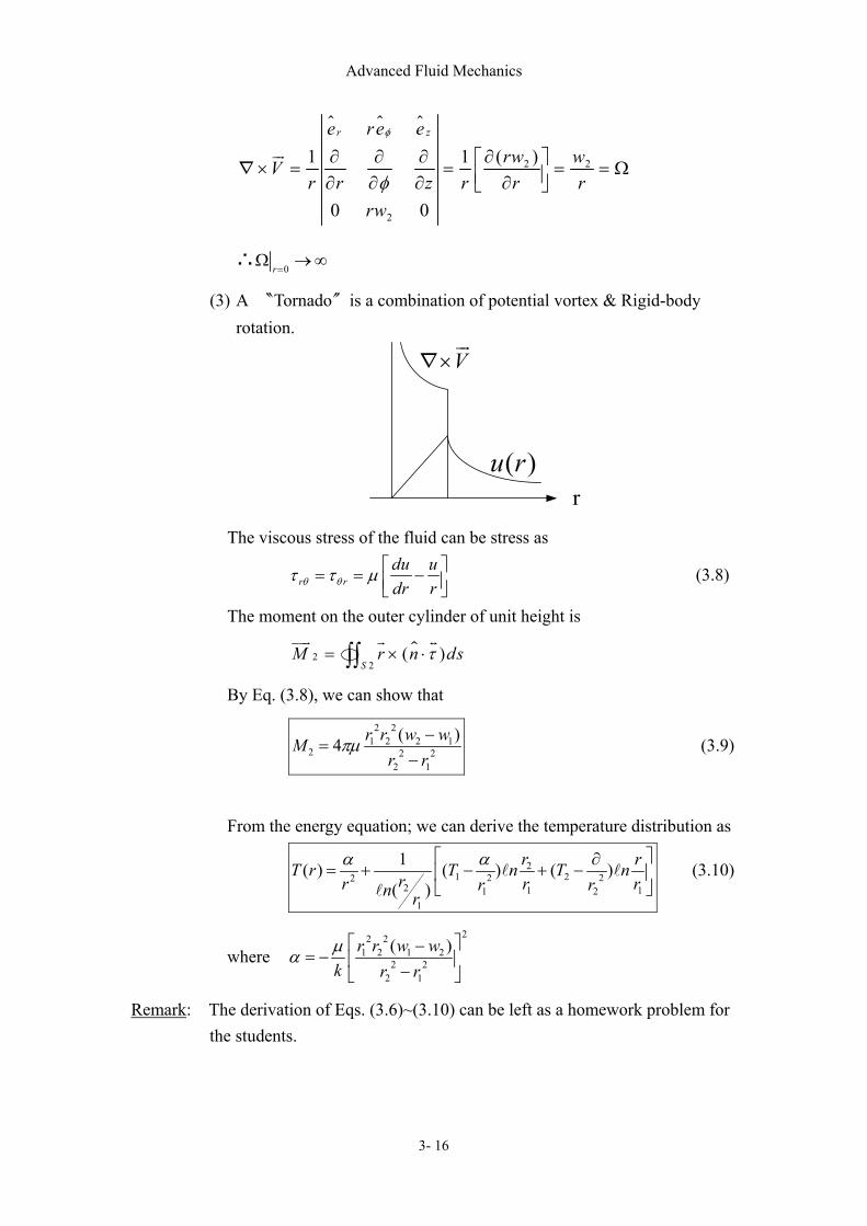
(3) A 〝Tornado〞is a combination of potential vortex & Rigid-body rotation.
V×∇
( )u rr
The viscous stress of the fluid can be stress as
r rdu udr rθ θτ τ µ = = −
(3.8)
The moment on the outer cylinder of unit height is
22
( )S
M r n dsτ= × ⋅∫∫
By Eq. (3.8), we can show that
2 21 2 2 1
2 2 22 1
( )4 r r w wMr r
πµ −=
− (3.9)
From the energy equation; we can derive the temperature distribution as
21 22 22
2 1 11 21
1( ) ( ) ( )( )
r rT r T n T nrr r rr rn r
α α ∂= + − + −
(3.10)
where 22 2
1 2 1 22 2
2 1
( )r r w wk r rµα −
= − −
Remark: The derivation of Eqs. (3.6)~(3.10) can be left as a homework problem for the students.
Advanced Fluid Mechanics
3- 17
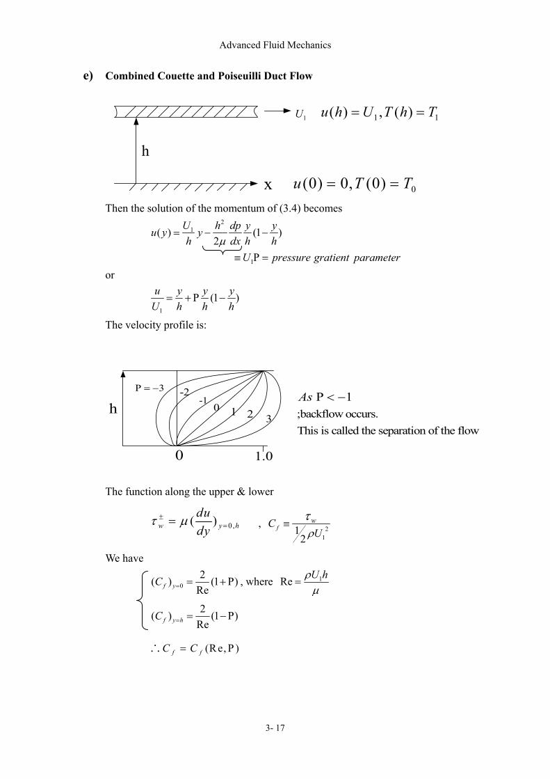
e) Combined Couette and Poiseuilli Duct Flow
1 1( ) , ( )u h U T h T= =
0(0) 0, (0)u T T= =
1U
h
x
Then the solution of the momentum of (3.4) becomes 2
1( ) (1 )2
U h dp y yu y yh dx h hµ
= − −
1U pressure gratient parameter≡ Ρ = or
1
(1 )u y y yU h h h
= + Ρ −
The velocity profile is:
3Ρ = −1As Ρ < −
;backflow occurs. This is called the separation of the flow
h
1.00
-2-1
0 1 2 3
The function along the upper & lower
0,( )w y hdudy
τ µ±== , 2
11
2f
wCUρ
τ≡
We have
02( ) (1 )
Ref yC = = + Ρ , where 1Re U hρµ
=
2( ) (1 )Ref y hC = = −Ρ
∴ (Re, )f fC C= Ρ

Advanced Fluid Mechanics
3- 18
In general:
(Re, , , Pr)pwf f
w
CTC CT k
µ+
−= Ρ =
(If consider conductivity) If the flow is compressible, connected with the energy equation
For the energy equation, if we assume also T=T(y) only, then
20 1
1 0 1 0
1 (1 )2 ( )
T T y U y yT T h h T T h h
µ−= + −
− −
21
0
Pr( )
p
p
C U Eck C T
µ= × ≡ ⋅
Where ( 0 1 0T T T≡ − )
.Pr PrandtlpNo
C viscous diffusion ratek thermal diffusion rate
µ≡ ≡ =
22ad1
0 0 0
2( T)Eckert No. = ( 1)( ) ( ) ( )p
U TEc r MC T T T
∞≡ ≡ = − , M→Mach No.
≈ work of compression (or the absolution temperature of the free stream)/(temperature difference) (Ec is important when the velocity is comparable with sound speed.)
also yh
η =
then 0
1 0
1 Pr (1 )2
T T EcT T
η η η−= + ⋅ −
−
yh
Pr 0Ec⋅ =
0
1 0
T TT T
−−
1 4 8

Advanced Fluid Mechanics
3- 19
3.2 Simple Unsteady Flow Assumptions: (1) Constant density, constantρ =
(2) , , kµ λ constants
(3) planar parallel flow 0z∂=
∂, 0v w= =
With the assumption above, we can only have ( , , )u u t x y= , ( , , )p p t x y= , ( , , )T T t x y=
By continuity equation: 0ux∂
=∂
⇒ ( , )u u t y=
By y-momentum equation: 0py∂
=∂
⇒ ( , )p p t x=
By x-momentum & continuity: 2
2 0px
∂=
∂ ⇒ ( )p fn t
x∂
=∂
only
∴ ( )p fn tx∂
=∂
(3.11)
The x-momentum and energy equations become 2
2
1u dp ut dx yρ
∂ ∂= − +
∂ ∂ν (3.12)
2 22
2 2( ) ( ) ( )vT T u T TC u kt x y x y
ρ µ∂ ∂ ∂ ∂ ∂+ = + +
∂ ∂ ∂ ∂ ∂ (3.13)
3.2.1 Stokes First problem (Rayleigh’s problem) Consider a semi-infinite space, y 0≥
y
x The air (or any medium) is still for 0y ≥ , t < 0. At t = 0, become wall impulsively moves to speed U0
0U
( , 0)U t y =
t
Advanced Fluid Mechanics
3- 20
The question is: What is the subsequent motion for y>0, and t>0 ?
First of all, we notice that there is 2 equations ((3.12) & (3.13)) but 3 unknown (p,
u, T). One unknown should be removed first. From Eq. (3.11), we have get ( )dp fn tdx
=
only, i.e. at a certain time (a fixed time) the value of dpdx
is not a function of position,
or the value of dpdx
is the same at any point of the flow domain. For our problem, as
y →∞ , u should approach to zero velocity for t >0, therefore, 2
2 0y y y
u u ut y y→∞ →∞ →∞
∂ ∂ ∂= = =
∂ ∂ ∂
Eqn (3.12) ⇒
2
2
1
y y y
u dp ut dx yρ→∞ →∞ →∞
∂ ∂= − +
∂ ∂ν
⇒ 0y
dpdx →∞
=
From our arguments that dpdx
is not a function of position, hence
0dpdx
= everywhere (3.14)
And the momentum equation becomes 2
2
du udt y
∂=
∂ν (3.15)
with B.C.’S 0( , 0)u t y U= = ( , ) 0u t y →∞ =
Eg. (3.15) is a P.D.E, we try to change it into a O.D.E, which will be easier to be
solved. Sinceν is a constant, Eq.(3.15) become
2
2( )u u
t y∂ ∂
=∂ ∂ν
Advanced Fluid Mechanics
3- 21
the independent variables are tν and y, therefore, a new variable should contain this
two parameters. Furthermore, we want the new variable to be dimensionless. In this
way, if we also set a new dependent variable to replace the old dependent variable u,
the equation will be dimensionless. We therefore can solve the O.D.E easier and once
for ever. Thus, define
( )y tα βη = ν , 0
( )u fu
η=
try the dimensional analysis
[ ] [ ]
22
3
uy
F L MLL LTL FLTT TM M M
L
τµρ ρ
∂∂
⋅
⋅ = = = = =
ν
2LT=
[ ] 2L=νt , [ ] L=y
So if want to dimensionlizeη , we should Take
1∂ = & 12
β = −
Thus 2
yη =νt
(3.16)
Recall
0
( )u fu
η= (3.17)
0 ( )u U f η=
12 22
yt t tη η∂ −= − =
∂ νt , 1
2yη∂=
∂ νt
0 0 2u df dfU Ut d t d t
η ηη η
∂ ∂= = −
∂ ∂
0 01
2u df dfU Uy d y d
ηη η
∂ ∂= =
∂ ∂ νt
2 2
02 2
14
u d fUy dη∂
=∂ νt
The coefficient 2 in the denominator is taken to make the final O.D.E. more easier to be integrated

Advanced Fluid Mechanics
3- 22
Eq. (3.15) ⇒ 2
0 2
12 4
df d fUd t d
ηη η
− = 0νUνt
⇒ 2
2 2 0d f dfd d
ηη η
+ = (3.18)
with B.C’S: 1 0η = , (0) 1f =
2 η →∞ , ( ) 0f ∞ =
Eq. (3.18) ⇒ '
'' 2 0df f
fη+ =
⇒ '
' 2df df
η η= −
⇒ ' 21 n f Cη= − +
or 2'f Ae η−=
integrate again
2
f A e d Bη η−= +∫
1 0η = , (0) 1f = 20 -
01=A e d Bη η +∫ ∴ B=1
2 η →∞ , ( ) 0f ∞ =
2-
00=A e 1dη η
∞+∫ ∴
2-z
0
1 1
e 2
Adz π∞
− −= =∫
∴ 22( ) 1f e dηη η
π−= − ∫
or 2
0
2( ) 1 zf e dzη
ηπ
−= − ∫ (3.19a)
( )erf η
Advanced Fluid Mechanics
3- 23
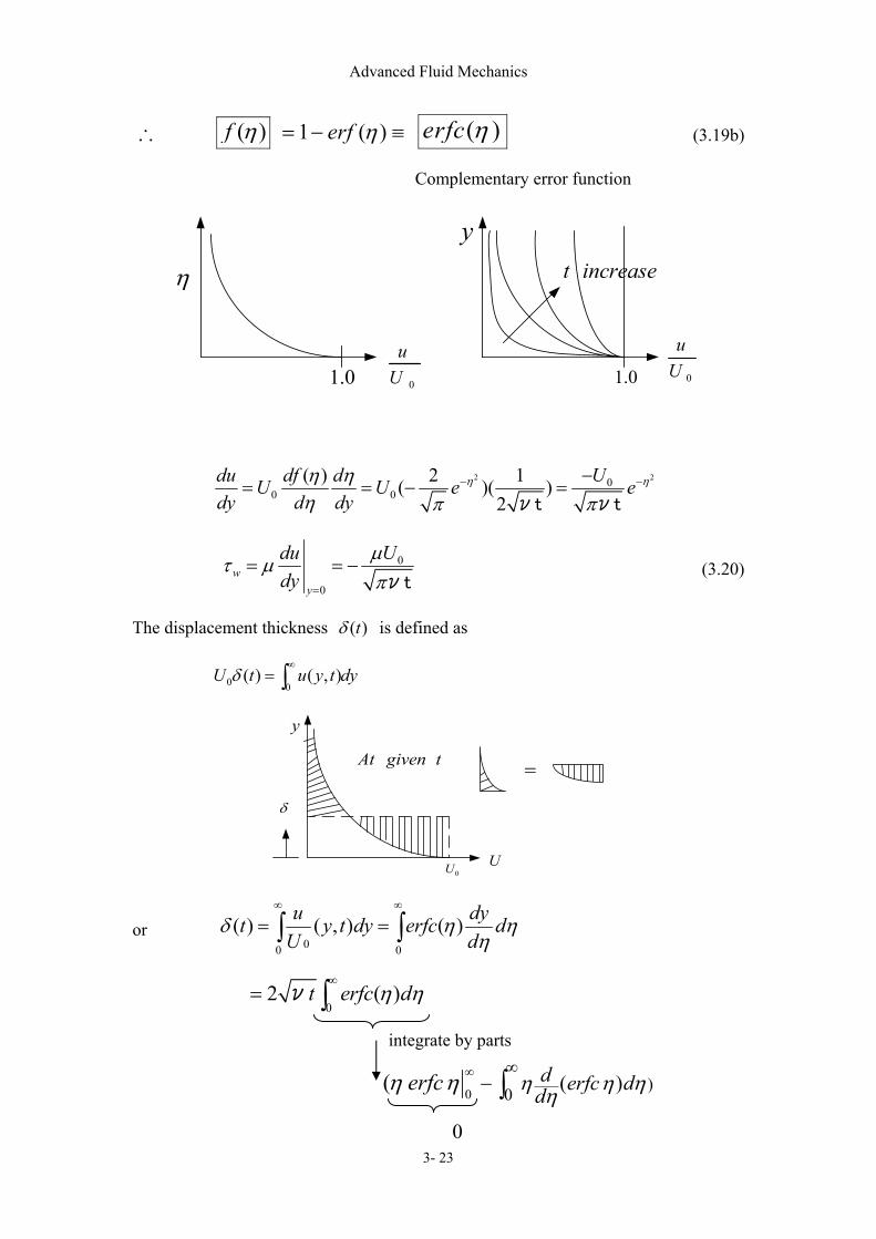
∴ ( )f η 1 ( )erf η= − ≡ ( )erfc η (3.19b)
Complementary error function
η
0
uU 0
uU
t increase
1.01.0
y
2 200 0
( ) 2 1( )( )2
Udu df dU U e edy d dy
η ηη ηη π π
− −−= = − =
νt νt
0
0w
y
Ududy
µτ µπ=
= = −νt
(3.20)
The displacement thickness ( )tδ is defined as
0 0( ) ( , )U t u y t dyδ
∞= ∫
0U
δ
=At given t
U
y
or 00 0
( ) ( , ) ( )u dyt y t dy erfc dU d
δ η ηη
∞ ∞
= =∫ ∫
02 ( )t erfc dη η
∞= ∫ν
integrate by parts
0)0 ( )( d erfc dderfc η η ηηη η ∞ ∞
− ∫
0

Advanced Fluid Mechanics
3- 24
η
( )erf η
η
( ) 1 ( )erfc erfη η= −
2
1
2( ( )) ( ) 2d erfc df e
d dηη η
η η π−= = −
2
0
2( ) 2 ( )t t e dηδ η ηπ
∞ −∴ = − −∫ν
2 2 2
0 02 2 2 ( )t te d e dη ηη η η
π π∞ ∞− −= =∫ ∫
ν ν
2
02 2t te η
π π
∞− = − =
ν ν (3.21)
for example: at t=10 sec
ν(m2/s) δ (m) µ (Pa Sec) Air,40 1.71×10⁻⁵ 0.0147 17.1 Water, 6.61×10⁻⁷ 0.0029 655
Lubricating Oil, 1×10⁻⁴ 0.0357 ---------------- Remark: At the first glance, it seems strength that the strength of the momentum
transport (or the speed of the propagation of the external disturbance) in three different fluid is:
Oil > Air > water While the µ of there is in the order of
Oil > water > Air
However, it is reasonable, since δ ~ ν1/2 ~ρµ , not only depend onµ .
Kg/m s
Advanced Fluid Mechanics
3- 25
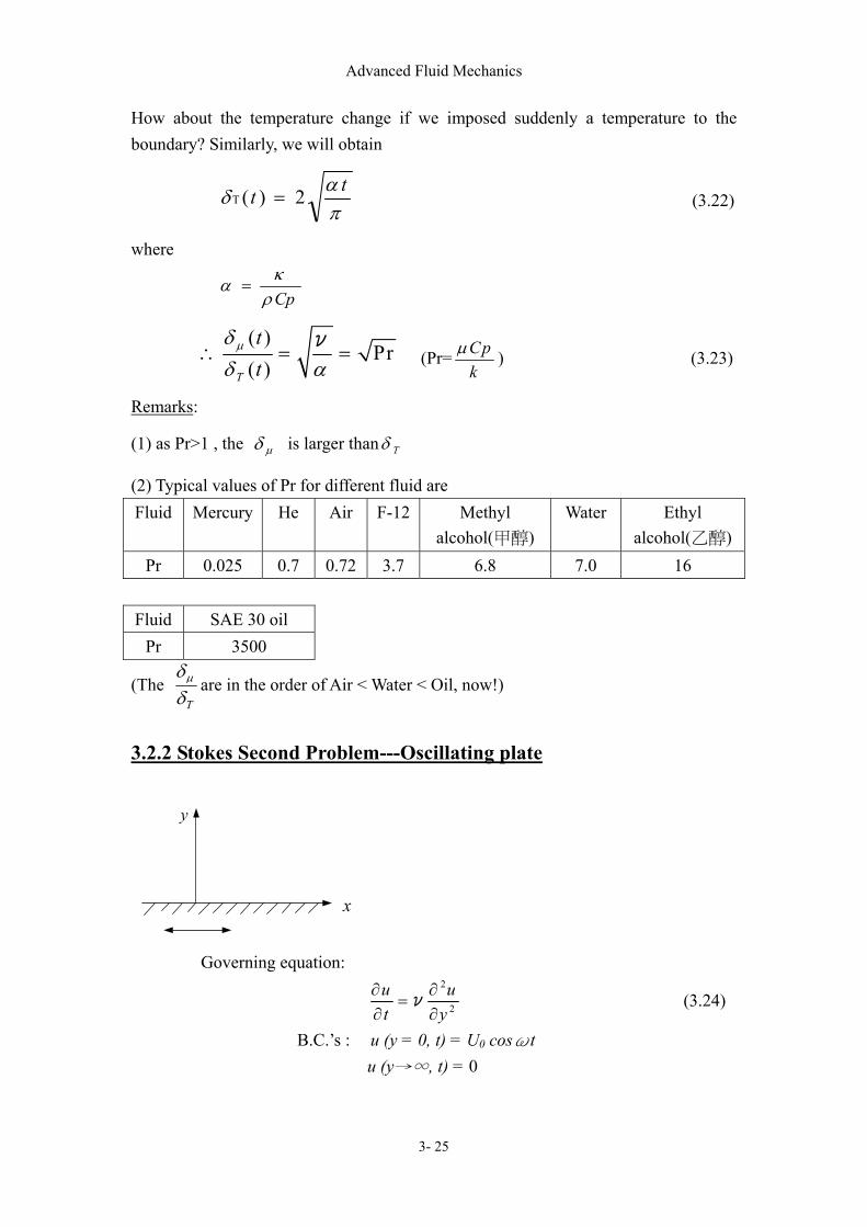
How about the temperature change if we imposed suddenly a temperature to the boundary? Similarly, we will obtain
παδ tt 2)( =Τ (3.22)
where
Cpρκα =
( )Pr
( )T
tt
µδδ α
∴ = =ν
(Pr= Cpk
µ ) (3.23)
Remarks:
(1) as Pr>1 , the µδ is larger than Tδ
(2) Typical values of Pr for different fluid are Fluid Mercury He Air F-12 Methyl
alcohol(甲醇) Water Ethyl
alcohol(乙醇)Pr 0.025 0.7 0.72 3.7 6.8 7.0 16
Fluid SAE 30 oil
Pr 3500
(The T
µδδ
are in the order of Air < Water < Oil, now!)
3.2.2 Stokes Second Problem---Oscillating plate
x
y
Governing equation:
2
2
u ut y
∂ ∂=
∂ ∂ν (3.24)
B.C.’s : u (y = 0, t) = U0 cosωt u (y→∞, t) = 0

Advanced Fluid Mechanics
3- 26
It is convenient (and make the procedure easier) to use a complex variable to solve the problem. Furthermore, if we are doing the problem of 0(0, ) sinu t U wt= , we can take the imaginary part of the solution and it is no need to do the problem twice.
sini te cos t i tω ω= +∵
we take the B.C. as
0( 0 , ) i tu t U e ω= (3.25)
Use separation of variables, we assume
0( , ) ( )i tu y t U e f yω= (3.26)
Eg.(3.25) of B.C. under thesolution theisWhich
Eg.(3.26). ofpart real thebe willproblem thisfosolution The :Note
0
2
0 02,
i t
i t i t
u i U e ftu uU e f U e fy y
ω
ω ω
ω∂=
∂∂ ∂′ ′′= =∂ ∂
sub into egn.(3.24) yields:
0 0i i ti U e f U e fω ωω ′′=ν
0if fω′′ − =ν
(3.27)
Use characteristic equation to solve, i.e. we assume
2,y y yf e f e f eλ λ λλ λ′ ′′= ⇒ = =
sub into Eg (3.27)
2
1/2
2 4
0
2 (1 )4 4 2
(1 )2
i i
i i
i e e cos i sin i
i
π π
ωλ λ
π π
ωλ
− = ⇒ = ±
= = = + = +
∴ = ± +
∵
ω
ν ν
ν
Advanced Fluid Mechanics
3- 27
(3.26)⇒
0 0
0
(1 ) (1 )2 2
( ) ( )2 2 2 2
( , )
i t i y i yyi t i t
y i t y y i t y
u y t U e e U Ae Be e
U Ae e Be e
ω ωωλω ω
ω ω ω ωω ω
+ + − +
+ − −
= = +
= +
ν ν
ν ν ν ν
Also 0 0(0, ) 1i t i tu t U e BU e Bω ω= = ⇒ =
Thus
0
( )2 2( , )
wy i t yu y t U e e
ω ω− −= ν ν
0 2 ( ) ( )2 2
yU e cos t y i sin t y
ω ω ωω ω−
= − + −
ν ν ν
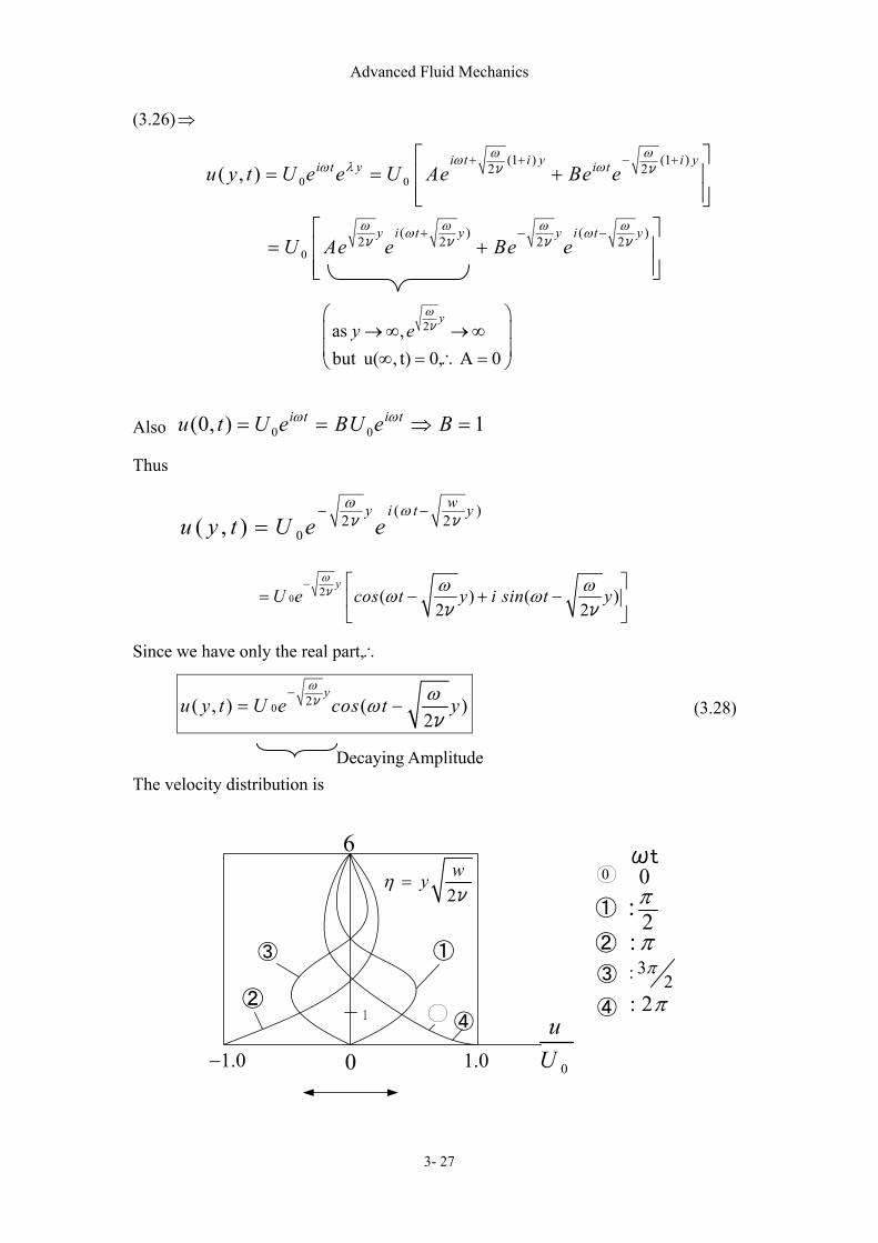
Since we have only the real part,∴
0 2( , ) ( )2
yu y t U e cos t y
ω ωω−
= −ν
ν (3.28)
Decaying Amplitude The velocity distribution is
2wyη =ν
0
uU
①③
②④
④
①
②
③
2:π
:π3: 2π
: 2π1
ωt
1.01.0−
600
0
2as ,but u( , t) 0, A 0
yy e
ω →∞ →∞
∞ = ∴ =
ν
Advanced Fluid Mechanics
3- 28
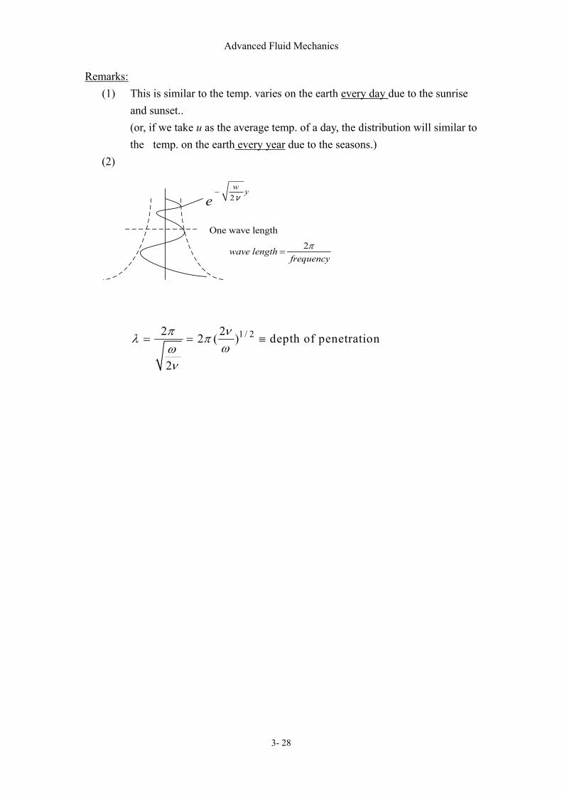
Remarks: (1) This is similar to the temp. varies on the earth every day due to the sunrise
and sunset.. (or, if we take u as the average temp. of a day, the distribution will similar to the temp. on the earth every year due to the seasons.)
(2)
2w y
e−
ν
2wave lengthfrequency
π=
One wave length
1 / 22 22 ( ) depth of penetration
2
π νλ πωω
ν
= = ≡
Advanced Fluid Mechanics
3- 29
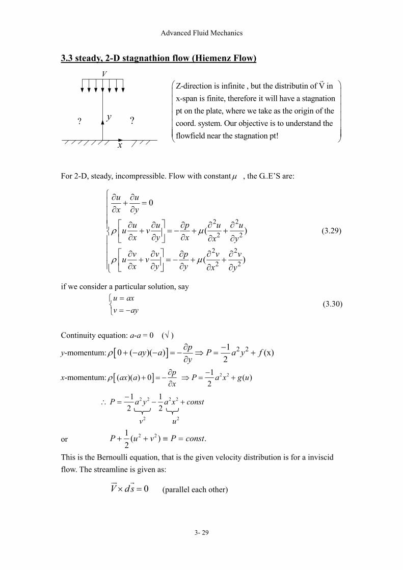
Z-direction is infinite , but the distributin of V inx-span is finite, therefore it will have a stagnationpt on the plate, where we take as the origin of the coord. system. Our objective is to understand the flowfield near the stagnation pt!
3.3 steady, 2-D stagnathion flow (Hiemenz Flow) V
y
x
? ?
For 2-D, steady, incompressible. Flow with constantµ , the G..E’S are:
2 2
2 2
2 2
2 2
0
( )
( )
u ux y
u u p u uu vx y x x y
v v p v vu vx y y x y
ρ µ
ρ µ
∂ ∂+ =
∂ ∂ ∂ ∂ ∂ ∂ ∂ + = − + + ∂ ∂ ∂ ∂ ∂ ∂ ∂ ∂ ∂ ∂ + = − + + ∂ ∂ ∂ ∂ ∂
(3.29)
if we consider a particular solution, say
−==
ayvaxu
(3.30)
Continuity equation: a-a = 0 (√ )
y-momentum: [ ] 2 210 ( )( ) (x)2
pay a P a y fy
ρ ∂ −+ − − = − ⇒ = +
∂
x-momentum: [ ] 2 21( )( ) 0 ( )2
pax a P a x g ux
ρ ∂ −+ = − ⇒ = +
∂
constxayaP +−−
=∴ 2222
21
21
2v 2u
or .)(21 22 constPvuP =≡++
This is the Bernoulli equation, that is the given velocity distribution is for a inviscid flow. The streamline is given as:
0V d s× = (parallel each other)
Advanced Fluid Mechanics
3- 30
0 ( ) 00
i j ku v udy vdx kdx dy
= − =
⇒ dx dyu v= ⇒ dx dy
ax ay=−
⇒ n x n y C= − +
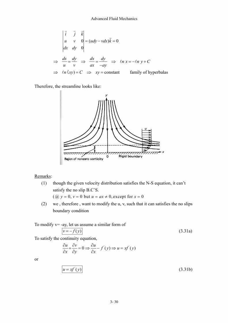
⇒ )n xy C= ( ⇒ constantxy = family of hyperbalas Therefore, the streamline looks like:
Remarks:
(1) though the given velocity distribution satisfies the N-S equation, it can’t satisfy the no slip B.C’S. ( @ 0, 0 but 0, except for 0y v u ax x= = = ≠ =
(2) we , therefore , want to modify the u, v, such that it can satisfies the no slips boundary condition
To modify v= -ay, let us assume a similar form of
( )v f y= − (3.31a) To satisfy the continuity equation,
' '0 ( ) ( )u v u f y u xf yx y x∂ ∂ ∂
+ = ⇒ − ⇒ =∂ ∂ ∂
or
' ( )u xf y= (3.31b)

Advanced Fluid Mechanics
3- 31
In order to satisfy the no-slip B.C’S:
'0
0 (0) 0y
u f== ⇒ =
00 (0) 0
yv f
== ⇒ = (3.32a, b)
As the ∞→y , we want u back to the inviscid case, that is u = ax, thus
' ( )f a∞ = (3.32c)
In the inviscid flow , the pressure is 2 2 2 20
12
p p a x a yρ = − +
Now, we modify the pressure as
2 2 20
1 ( )2
P P a x a F yρ = − + (3.33)
Not that u, v, p are replaced by two unknown function f (y) and F(y). However, we still have two momentum equations. the problem is closure. Sub. u, v, and p into the x-momentum equation, we have
2' '' 2 '''f ff a f− = +ν (3.34)
Sub u, v p∆ into y-momentum equation:
' 2 ' ''12
ff a F f⇒ = -ν
or ' '' '2
2F f ffa
= + ν
or 2
'2
22fF f const
a
= + + ν (3.35)
In summary, we have
2' 2''''' 0f ff f a+ − + =ν (3.34)
2'
2
22fF f const
a
= + + ν (3.35)
with B.C’S. 1 0)0( =f 2 ' (0 ) 0f = 3 ' ( )f a∞ =
Advanced Fluid Mechanics
3- 32
η
' uU
φ =
vφ ∼
1.0
with eq.(3.34) and B.C’S, we can solve the unknown function f. We want to use similarity method, introduce
yη α= , ( ) ( )f y Aφ η= then
23 2 2 2 ' 2'''''' 0( )( )A aA A Aα φ φ α φφ α + =+ −ν
2 2 ''A α φφ
To let the equation non-dimensionalized, i.e., let the coefficients of the above equation become all identically equal to unity , we put
3 2A aα =ν and 2 2 2A aα =
∴ A a= ν and α =a
ν
Thus, the new independent variables are a yη =ν
, ( ) ( )F y aφ η= ν (3.36)
The G.E’s become 2
' '
'''' '' 1 0:(0) 0, (0) 0, ( ) 1
with sφ φφ φ
φ φ φ
+ − + =
= = ∞ =
'
B.C
(3.37)
⇐Hiemenz Flow also get
2 '( 2 )Faφ φ= +
ν (3.38)
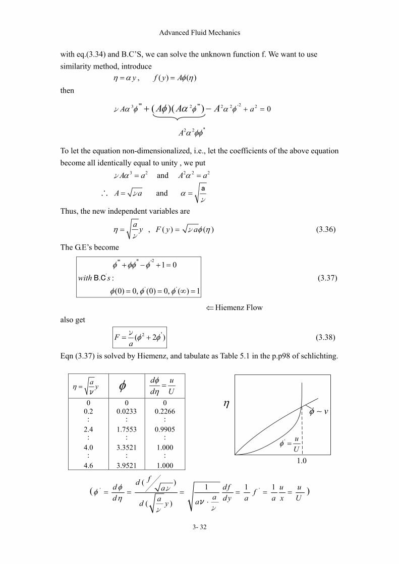
Eqn (3.37) is solved by Hiemenz, and tabulate as Table 5.1 in the p.p98 of schlichting.
a yη =ν
φ d ud Uφη=
0 0.2 : 2.4 : 4.0 : 4.6
0 0.0233 :
1.7553 :
3.3521 :
3.9521
0 0.2266 :
0.9905 :
1.000 :
1.000
( ' '( ) 1 1 1
( )
fdd d f u ua fad d y a a x Ua ad y
φφη
= = = = = =⋅ν
ν
νν
)
Advanced Fluid Mechanics
3- 33
jV
h
xy
d
Remarks: (1) As 9905.0/ ,4.2 == Uuη . We consider the corresponding distance from
the wall as the boundary layerδ , therefore ( a y ya
η η= =ν
ν)
2.4a aδδ η= =ν ν (3.39)
Note also that δ is independent of x. (The boundary-layer thickness is constant because the thinning due to stream acceleration exactly balances the thicknessing due to viscous dissipation)
2U ax=1U ax=
δ
1x
y
(2) As x →∞ , v ay= − & u →∞ for 0y ≠
As y →∞ (or η →∞ ), u ax= and v →∞ (∵φ →∞ ) That is the modified solution, though satisfies the no slip condition, still can’t satisfy the condition at infinite. We will see this problem in the “boundary layer theory”.
(Localized solution)
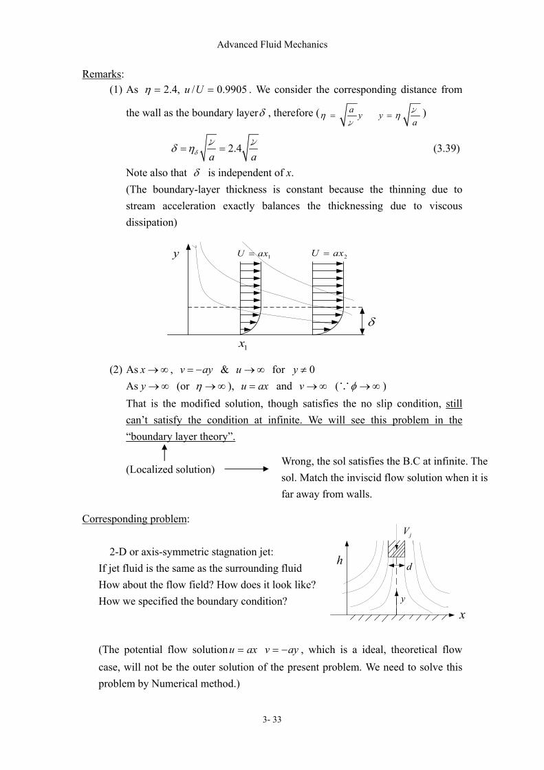
Corresponding problem:
2-D or axis-symmetric stagnation jet:
If jet fluid is the same as the surrounding fluid How about the flow field? How does it look like? How we specified the boundary condition? (The potential flow solution ayvaxu −== , which is a ideal, theoretical flow case, will not be the outer solution of the present problem. We need to solve this problem by Numerical method.)
Wrong, the sol satisfies the B.C at infinite. The sol. Match the inviscid flow solution when it is far away from walls.

Advanced Fluid Mechanics
3- 34
2-D or axis-symmetric Spraying.
jV
Liquid fuel
Air
x
How does the spray looked like?
Advanced Fluid Mechanics
3- 35
θ
,ze w
,e vθ
Z
y
x
r
ω
uer ,ˆ
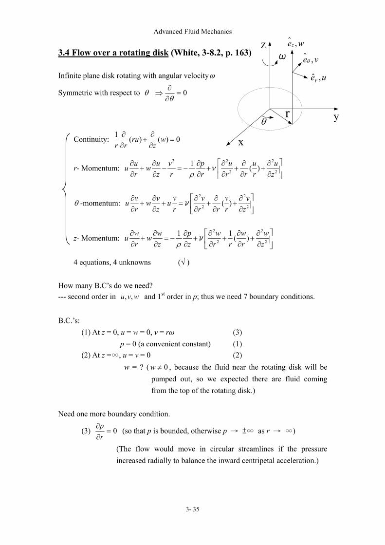
3.4 Flow over a rotating disk (White, 3-8.2, p. 163) Infinite plane disk rotating with angular velocityω
Symmetric with respect to θ 0=∂∂
⇒θ
Continuity: 1 ( ) ( ) 0ru wr r z∂ ∂
+ =∂ ∂
r- Momentum: 2 2 2
2 2
1 ( )u u v p u u uu wr z r r r r r zρ
ν ∂ ∂ ∂ ∂ ∂ ∂+ − = − + + + ∂ ∂ ∂ ∂ ∂ ∂
θ -momentum: 2 2
2 2( )v v v v v vu w ur z r r r r z
∂ ∂ ∂ ∂ ∂+ + = + + ∂ ∂ ∂ ∂ ∂
ν
z- Momentum: 2 2
2 2
1 1 ( )w w p w w wu wr z z r r r zρ
∂ ∂ ∂ ∂ ∂ ∂+ = − + + + ∂ ∂ ∂ ∂ ∂ ∂
ν
4 equations, 4 unknowns (√ ) How many B.C’s do we need? --- second order in wvu ,, and 1st order in p; thus we need 7 boundary conditions. B.C.’s:
(1) At z = 0, u = w = 0, v = rω (3) p = 0 (a convenient constant) (1)
(2) At z =∞, u = v = 0 (2) w = ? ( 0≠w , because the fluid near the rotating disk will be
pumped out, so we expected there are fluid coming from the top of the rotating disk.)
Need one more boundary condition.
(3) 0=∂∂
rp (so that p is bounded, otherwise p → ±∞ as r → ∞)
(The flow would move in circular streamlines if the pressure increased radially to balance the inward centripetal acceleration.)

Advanced Fluid Mechanics
3- 36
Compare inertial & viscous term in the r-momentum: 2
2
u uur z∂ ∂∂ ∂∼ν
[ ]12 2( )( ) ( ) / ( )O r O r δ δ ⇒ ∼ ∼ νω ω νω
ω
Therefore, we may non-dimensional z by the use ofδ . Introduce a new variable 1
2( )z zζδ
= =ω
ν (White: z*)
Also, try to use separation variables method by assuming
u = ω r F( ζ ) v = ω r G( ζ )
w = 1
2( )ων H( ζ )← function of z only since r & z are assumed separated
p = ρν ω P( ζ ) ← Since 0 is function of onlyp p zr∂
= ∴∂
)
The B.C.’s become: ζ= 0, F(0) = H(0) = P(0) = 0, G(0) = 1 (z = 0)
ζ =∞, F(∞) = G(∞) = 0 (z→∞) (3.40)
( 0=∂∂
rp cancel one term in r-momentum equation!) (3-185)
The G.E.’s becomes Continuity: 2F + H' = 0
r : F2 - G 2 + HF ' = F ''
θ : 2FG + HG '-G '' = 0 z : P ' + HH '-H '' = 0 (3.41a~d )
(3-184) Equation (3.41a-c) with B.C. (3.40) is sufficient to solve F, H, and G the results can be applied to equation (3.41d) to solve P. For small value of z, such that ζ is small seek a solution in powers of ζ
F = a0 +a1ζ + a2ζ 2 + a3ζ 3+ h.o.T neglecting high order terms
G = b0 +b1ζ +b2ζ 2 + b3ζ 3+ h.o.T
H = c0 +c1ζ +c2ζ 2 + c3ζ 3+ h.o.T (3.42)
(so that the effect of r and z are separated; u = vr; v = vq; w = vz)
Advanced Fluid Mechanics
3- 37
Try to determine 0 3,a c…… (12 unknowns)
From B.C’s on ζ = 0, F = 0 ⇒ a0 = 0 G = 1 ⇒ b0 = 1 H = 0 ⇒ c0 = 0
Apply the G.E. at ζ = 0, with F = H = 0 and G =1, we have
Continuity: 0 + H '(0) = 0 ⇒ H '(0) = 0 ⇒ c1 = 0
r: 0 – 1 + 0 = F ''(0) ⇒ F ''(0) = -1 ⇒ a2 = 21
−
θ: 0 + 0 - G ''(0) = 0 ⇒ G ''(0) = 0 ⇒ b2 = 0
Now differentiate original equations ω.r.t. ζ '
' ' ' '
'
''
'' '''
' ' ' '' '''
2 0
2 2 0
2 2 0
F H
FF GG H F HF F
F G FG H G HG G
+ =
− + + − =
+ + + − =
(3.43a-c)
Sub. (3.42) into (3.43) again for, ζ = 0, and use the previous results (i.e. a0 = 0, b0 = 0, c0 = 0, c1 = 0, a2 = -1/2, b2 = 0), we get
2a1 + 2c2 = 0
-2b1 – 6a3 = 0
2a1 – 6b3 =0 (3.44 a-c)
Differentiate Eq. (3.43a) again and evaluate at ζ = 0: 2F '' + H ''' = 0
(at ζ = 0, F '' = 2a2 = -1, H ''' = 3 4 306 24 ... 6c c c
ςς
=+ + = )
⇒ -2 + 6c3 = 0 ⇒ 31
3 =c
We have get 3+3+1=7 coefficients, therefore 5 unknowns left. However, we have 3 equations (Eq 3.44a-c), thus, we can express 3 unknown (c2, a3, b3) in terms of the other 2 unknowns (a1, b1). From (3.44) we have
C2 = -a1, a3 = -b1/3, b3 = a1/3
Advanced Fluid Mechanics
3- 38
The solution thus become
2 311
311
2 31
1 ....2 3
1 ......31 ......3
bF a
aG b
H a
ζ ζ ζ
ζ ζ
ζ ζ
= − − +
= + + +
= − + +
(3.45)
Two unknowns: 1a & 1b . Also note that Eq. (3.45) will not suitable for ζ→∞, because F, G, H will→∞ Now, let’s look at the equation. At ∞→ζ , where F(ζ ) = G(ζ )=0 is the known B.C.’s
Continuity: '2 0F H+ = ⇒ H '= 0 → H (ζ ) = -C (∵w < 0 at ζ→∞)
r : F2 - G 2 + HF ' = F '' ⇒ HF ' = F ''
θ : 2FG + HG '-G '' = 0 ⇒ HG '= G ''
' ' ( ) ( )H c cF e F e F eζ ζ ζζ ζ− −∞ ⇒ ∝ ⇒ ∝∼
' ' ( ) ( )c cHG e G e G eζ ζ ζζ ζ− −∞ ⇒ ∝ ⇒ ∝∼
Thus, in the far away region, we seek solution of the form of
F = A1e-cζ + A2e-2cζ +……
G = B1e-cζ + B2e-2cζ +…… (3.46)
H = – C + C1e-cζ + C2e-2cζ +…… Sub (3.46) into the G.E.s Continuity:
2A1e-Cζ + O[e-2Cζ] + … + – CC1e-Cζ + O[e-2Cζ] +…… = 0
⇒ e-Cζ: 2A1 – CC1 = 0 ⇒ C1 = 2A1/C
r-momentum:
A1e-Cζ + A2e-2Cζ2 – B1e-Cζ +…2 + [– C + C1e-Cζ +…][–A1Ce-Cζ
–2CA2e-2Cζ +…] = + A1C2 e-Cζ + 4C2A2C2 e-2Cζ +…
⇒ e-2cζ: A12 – B1
2 - CC1A1 + 2C2A2 – 4C2A2= 0
⇒ A2 = –2 2
1 12
(A +B )2C
⇒
Advanced Fluid Mechanics
3- 39
θ -momentum
B2 = 0 and C2 = –2 2
1 13
(A +B )2C
The solution near ζ→∞ is thus
F = A1e-Cζ + (A12 +B1
2) / 2C2e-2Cζ +……
G = B1e-Cζ + O[e-3Cζ] +…… (3.47)
H = – C + 12AC
e-Cζ – 2 2
1 13
(A +B )2C
e-2Cζ +……
Unknowns: A1, B1, C By matching the “inner” solution for small ζ to an “outer” solution for large ζ. That is, take small value of ζ in Eq. (3.47a). Numerically, we finally obtain
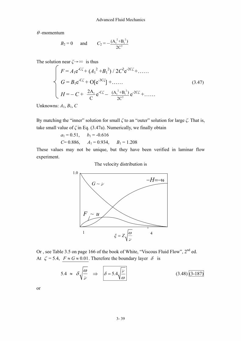
a1 = 0.51, b1 = -0.616 C= 0.886, A1 = 0.934, B1 = 1.208
These values may not be unique, but they have been verified in laminar flow experiment.
The velocity distribution is
1
0.1
4
~G νwH −=−
uF ~
Z ωξ =ν
Or , see Table 3.5 on page 166 of the book of White, “Viscous Fluid Flow”, 2nd ed. At ζ = 5.4, 0.01F G≈ ≈ . Therefore the boundary layer δ is
5.4 ≈ ωδν
⇒ 5.4δω
=ν (3.48) (3-187)
or
Advanced Fluid Mechanics
3- 40
δ
Z
rv ω=
δu
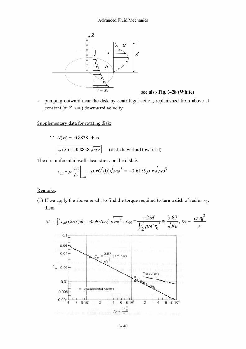
see also Fig. 3-28 (White) - pumping outward near the disk by centrifugal action, replenished from above at
constant (at Z→∞) downward velocity. Supplementary data for rotating disk:
∵ H(∞) = -0.8838, thus
vz (∞) = -0.8838 ων (disk draw fluid toward it)
The circumferential wall shear stress on the disk is
θ
0zθ
z
uz
µτ=
∂=
∂=
' 3 3 (0) 0.6159 rG rρ ω ρ ω= −ν ν
Remarks:
(1) If we apply the above result, to find the torque required to turn a disk of radius r0 . them
0
zθ0(2 )
rM r r drτ π= =∫ -0.967ρr0
4 3νω ; CM ≡ 520
2 3.871
2
MRerρω
−≅ , Re =
20 rω
ν

Advanced Fluid Mechanics
3- 41
The equation agrees well with experimental data for 53 10Re < ×
For 53 10Re < × , the flow becomes turbulent.
(2) If we stir tea in a cup; the flow pattern will be reversed. Thus these exists an
inversed radial flow.
(3) Rogers & Lance (1960) used a Runge-Kutta method to solve eqns (3.41), by
defining
Y1 = H, Y3 = F, Y5 = G
Y2 = 'F , Y4 = 'G , Y6 = Р
with I.C’s: Y1(0) = Y3(0) = Y6(0) = 0 , Y5(0) = 1 (3.40a)
The two unknown conditions of Y2 (0) & Y4 (0) must be chosen to satisfy the end
B.C.’s (3.40b). Namely
Y3 → 0, Y5 → 0, at ζ → ∞.
The fortrain statements for (3.41) are simply six statements, as described in p.165
of White’s book. By numerical iteration, we can find the I.C.’s to be
Y2 (0) = 'F (0) = 0.5102 Y4 (0) = 'G (0) = -0.6159
The numerical results agree well with those obtained by asymptotic expansion.

Advanced Fluid Mechanics
3- 42
5
5−
φ
100u
u
123456
7
3.5 Flow in a channel (3-8.3 Jeffery-Hamel Flow in a Wedge-Shaped Region)
α2φ φ
0u
(sink) convergent flow flow (source) divergent
1 2 3 4 5 6 7 The velocity distributions are Re = u0r /ν
1 : Re = 5000 2 : Re = 1342 convergent 3 : Re = 684
5 : Re = 684 6 : Re = 1342 divergent 7 : Re = 5000
Advanced Fluid Mechanics
3- 43
3.6 Stream Function For a 2-D, constant density flow (incompressible flow)
0=⋅∇ V ⇒ 0=∂∂
+∂∂
yv
xu ⇒ u =
y∂∂ψ ; v =
x∂∂
−ψ (3.49)
⇒ 0)()(22
=∂∂
∂−
∂∂∂
=∂∂
−∂∂
+∂∂
∂∂
yxyxxyyxψψψψ
By introducing the stream function “ψ”, the continuity equation is automatically satisfied. (By introducing theψ , the independent variable & the governing equation are reduced by one, however, the order of the P.D.E. increases by one.) In 3-D flow, the eqn of streamline is
0V d s× =
Where kwjviuV ˆˆˆ ++= , ˆ?d s dxi dyj dzk= + +
Thus udx =
vdy =
wdz
or dxdy =
),,(),,(
zyxuzyxv ,
dxdz =
),,(),,(
zyxuzyxw
The stream functions will be ψ 1(x,y,z) = C1 = constant, ψ 2(x,y,z) = C2 =constant
V1ψ∇
2ψ∇
y
z
x
const2 =ψ
const 1 =ψ
)line stream(
Since 21 ψψ ∇×∇ has the same direction as V , so we can say
V = k ( 21 ψψ ∇×∇ )
proportional constant
Advanced Fluid Mechanics
3- 44
Or
ҜV = 21 ψψ ∇×∇
Since
)( 21 ψψ ∇×∇⋅∇ = 0 (Mathematically)
∴ ⋅∇ (ҜV ) = 0
But for steady flow, we know 0)Vdiv( =ρ , so we can pick up Ҝ = ρ, then
ρV = 21 ψψ ∇×∇ (3.50)
If the flow is constant density, we know 0)Vdiv( =ρ , so we can pick up Ҝ = 1, then
V = 21 ψψ ∇×∇ (3.51)
Remarks:
There are only a few exact solutions for N-S equation unless the physical
problem and geometry is easy. The N-S equation may be simplified as Re >>1 or Re
→ ∞, where the exact solution may also be exist. In the next two chapters, we will
consider the flow fluid when Re >>1 or Re → 0.
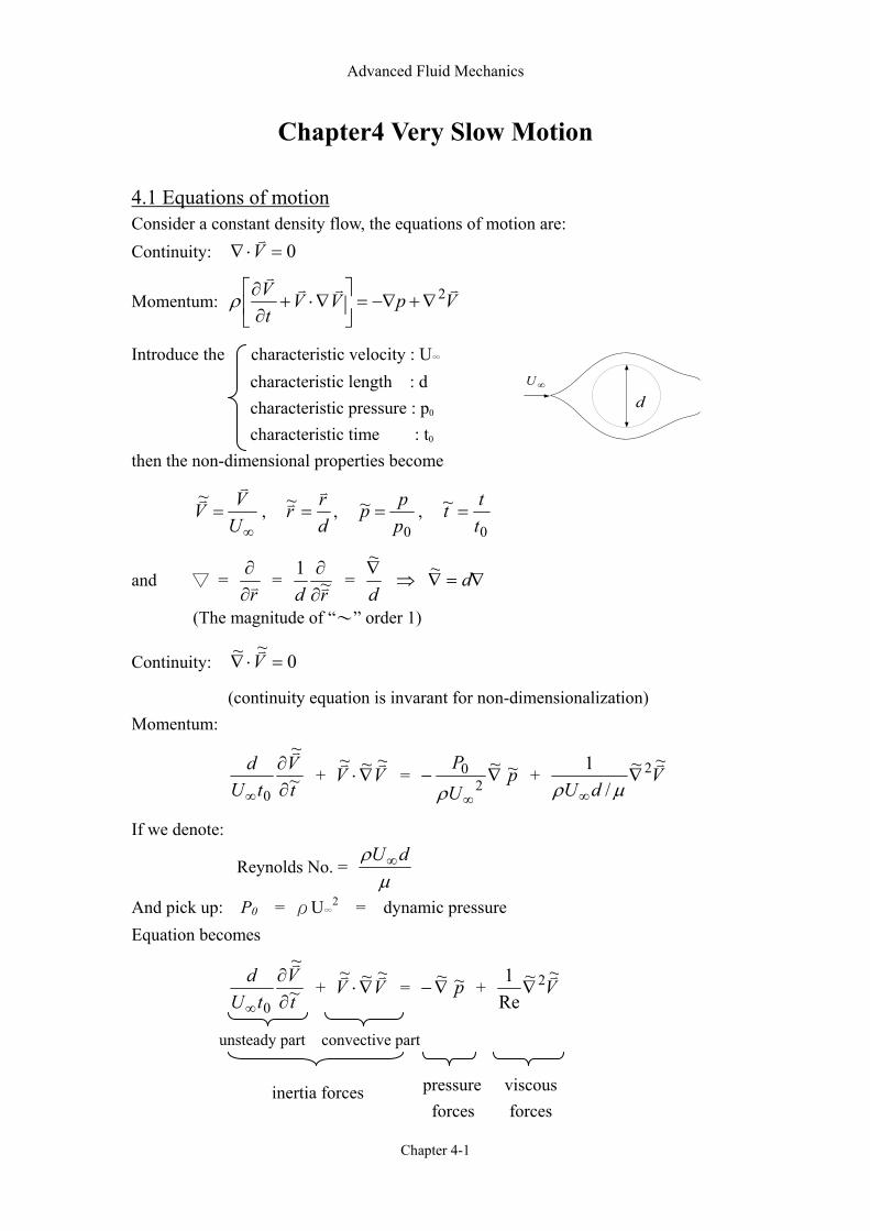
Advanced Fluid Mechanics
Chapter 4-1
d∞U
Chapter4 Very Slow Motion 4.1 Equations of motion Consider a constant density flow, the equations of motion are: Continuity: 0=⋅∇ V
v
Momentum: VpVVtV vvvv
2∇+−∇=
∇⋅+
∂∂ρ
Introduce the characteristic velocity : U∞ characteristic length : d characteristic pressure : p0
characteristic time : t0
then the non-dimensional properties become
∞=
UVVv
v~,
drrv
v =~ , 0
~ppp = ,
0
~ttt =
and = rv∂∂
= rd ~
1v∂∂
= d∇~
⇒ ∇=∇ d~
(The magnitude of “〜” order 1)
Continuity: 0~~ =⋅∇ Vv
(continuity equation is invarant for non-dimensionalization) Momentum:
tV
tUd
~
~
0 ∂∂
∞
v
+ VV~~~ vv
∇⋅ = pUP ~ ~
20 ∇−∞ρ
+ VdU
~~/
1 2 v∇∞ µρ
If we denote:
Reynolds No. = µ
ρ dU∞
And pick up: P0 = ρU∞2 = dynamic pressure
Equation becomes
tV
tUd
~
~
0 ∂∂
∞
v
+ VV~~~ vv
∇⋅ = p~ ~∇− + V~~
Re1 2 v∇
unsteady part convective part
inertia forces pressure
forces viscous forces

Advanced Fluid Mechanics
Chapter 4-2
1) If Re→∞ ⇒ tV
tUd
~
~
0 ∂∂
∞
v
+ VV~~~ vv
∇⋅ = p~ ~∇− (4.1)
2) If Re→ 0 ⇒ 0~ 2 =∇ Vv
(4.2)
Note that there is no balance term. We want to have a balance term. Multiply (4.11) by Re
RetV
tUd
~
~
0 ∂∂
∞
v
+ Re VV~~~ vv
∇⋅ = pUP ~ ~
20 ∇−∞
Reρ
+ V~~ 2 v∇
(0, as Re→0) (i) The unsteady term coefficient:
For a oscillation body flow, w = frequency of oscillation
we can choose: t0 = ω1
the first coefficient:
Re0tU
d
∞ = Re
∞Udω
→ 0, as Re → 0 and ω is not very large
Remark: 1 if there is no body oscillation, we may pick t0 = U∞/d 2 For a highly oscillation body, the unsteady term can’t neglected.
(ii) The pressure coefficient
We want to pick up P0 such that Re2
0
∞U
P
ρ→ 1, and this term can be left to
balance the viscous term. Therefore
P0 = Re
2∞Uρ
= µρ
ρ/
2
dUU
∞
∞ = dU∞µ
And the momentum equation (4.1) become
0 = p~ ~∇− + V~~ 2 v∇ (4.3)
Summary: For a steady, constant density, slow flow (Re→0)
V~~ v
∇ = 0
0 = p~ ~∇− + V~~ 2 v∇
Also name as: Slow flow, Creeping flow, or stokes′flow.
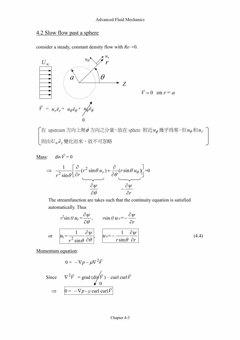
Advanced Fluid Mechanics
Chapter 4-3
4.2 Slow flow past a sphere consider a steady, constant density flow with Re→0.
Zθa
rθu ru
∞U
Vv
= rreu v + θθ eu v + φφeu v
0
在 upstream 方向上無φ 方向之分量,故在 sphere 附近 φu 幾乎為零。但 θu 和 ru
則由 zeU ˆ∞ 變化而來,故不可忽略
Mass: divV
v= 0
⇒
∂∂
+∂∂ ) sin() sin(
sin1 2
2 θθθ
θθ
ururrr
r =0
θψ∂∂
r∂
∂−
ψ
The streamfunction are takes such that the continuity equation is satisfied automatically. Thus
r2sinθur = θψ∂∂
, rsinθuθ=r∂
∂−
ψ
or ur = θψ
θ ∂∂
sin1
2r, uθ=
rr ∂∂
−ψ
θsin1
(4.4)
Momentum equation:
0 = Vpv2∇−∇− µ
Since Vv2∇ = grad (divV
v) – cuel curlV
v
⇒ 0 = p∇− -μcurl curlVv
0=Vv
on r = a
0

Advanced Fluid Mechanics
Chapter 4-4
take curl on both side
0 = 0 -μcurl curl curlVv
(4.5)
Ω≡v
Ωv
= cuelVv
= θsin
12r
0
ˆ sinˆˆ
θ
φθ
φθ
θ
ruur
erere
r
r
∂∂
∂∂
∂∂
= θsin
12r
∂∂
−∂
∂++
θθ θ
φθr
ru
rru
eree)(ˆ sin)0(ˆ)0(ˆ
=
∂∂
−∂∂
+θ
θθ
φ rur
uru
re
sub. Eqn (4.4)
= r
eφˆ
∂∂
∂∂
−∂∂
−∂∂
+∂∂
− )sin1()
sin1(
sin1
2 θψ
θθψ
θψ
θ rrrrr
rr
= r
eφˆ
∂∂
∂∂
−∂
∂+
∂∂−
−∂∂
− )sin
1(1)11(sinsin
122
2
2 θψ
θθψψ
θψ
θ rrrrrr
rr
=
∂∂
∂∂
+∂
∂−)
sin1(sin
sinˆ
22
2
θψ
θθθψ
θφ
rrre
= Ω φe
Where Ω ≡θsin
1r
− Dψ
D ≡ differential operator ≡ 2
2
r∂∂
+ )sin
1(sin2 θθθθ
∂∂
∂∂
r
Then
Curl Ωv
=θsin
12r
Ω∂∂
∂∂
∂∂
00
ˆ sinˆˆ
φθ
θ φθ
r
ererer
=θsin
12r
∂Ω∂
−∂Ω∂
rerer θθˆˆ

Advanced Fluid Mechanics
Chapter 4-5
Finally, we can obtain
curl curlΩv
= θ
φ
sinˆ
re
D2ψ
Eq. (4.5) ⇒ D2ψ = 0
or
∂
∂2
2
r+
2
2 )sin
1(sin
∂∂
∂∂
θθθθ
rψ =0 (4.6)
B.C’S in terms of ψ : (Recall ur = θψ
θ ∂∂
sin1
2r, uθ=
rr ∂∂
−ψ
θsin1
)
(i) On r = a:
ur = 0 → θψ∂∂
= 0
uθ= 0 → r∂
∂ψ = 0 (4.7a)
(ii) Infinity condition
∵ ∞Vv
= U∞ ze = U∞[( cosθ) re + (-sinθ) θe ]
∴ ur = θψ
θ ∂∂
sin1
2r → U∞cosθ as r→∞ (4.8a)
uθ= rr ∂
∂−
ψθsin
1 → -U∞sinθ as r→∞ (4.8b)
integrate (4.8a) and (4.8b), we obtain
ψ ~ U∞ 2
2r sin2θ as r→∞ (4.7b)
Assume: ψ (r,θ) = f(r)sin2θ, then the B.C’S become
(4.7a) r = a → )(' af = f (a) = 0
(4.7b) r→∞ → f (r) ~ U∞
2
2r as r→∞
Advanced Fluid Mechanics
Chapter 4-6
Sub. Into Eq. (4.6), we get
0)2)(2()2( 22
2
22
22
22
2=−−=−
rf
drfd
rdrdf
rdrd
Aside: 02
22
3
33
4
44 =++++ df
drdfcr
drfdbr
drfdar
drfdr
we can assume solution to be the form of f = Arn,
we will have 4 roots for n, n= 1, -1, 2, 4.
∴ f = rA
+ Br + Cr2 +Dr4 (4.9)
B.C’S:
(1) f (r) ~2
2rU∞ as r→∞
compare with (4.9), we observe that we need to take C = 2∞U
and D = 0
to satisfy f (r) ~2
2rU∞ for r →∞. ( The value of A, B are not important,
since they are not the highest order term, and r2 >> r as r→∞) Eq. (4.9) ⇒
f = rA
+ Br +2∞U
r2 (4.10)
(2) f (a) = 0 → aA
+ Ba +2∞U
a2 = 0
)(' af = 0 → - 2Aa
+ B + U∞ a = 0
A =41 a3U∞ , B =
43
− aU∞
∴ ψ (r,θ) = a2 U∞ sin2θ
+− 2)(
21)(
43)(
41
ar
ar
ra
+ const (4.11a)
ur = U∞cosθ
+− 3)(
21)(
231
ra
ra
uθ= -U∞sinθ
−− 3)(
41)(
431
ra
ra
(4.11 b, c)
⇒
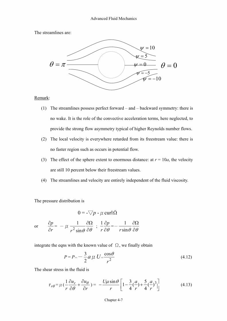
Advanced Fluid Mechanics
Chapter 4-7
The streamlines are:
πθ = 0=θ0=ψ5=ψ
10=ψ
5−=ψ10−=ψ
Remark:
(1) The streamlines possess perfect forward – and – backward symmetry: there is
no wake. It is the role of the convective acceleration terms, here neglected, to
provide the strong flow asymmetry typical of higher Reynolds number flows.
(2) The local velocity is everywhere retarded from its freestream value: there is
no faster region such as occurs in potential flow.
(3) The effect of the sphere extent to enormous distance: at r = 10a, the velocity
are still 10 percent below their freestream values.
(4) The streamlines and velocity are entirely independent of the fluid viscosity.
The pressure distribution is
0 = -p -μcurlΩv
or rp∂∂
= -μθθ ∂Ω∂
sin1
2r ;
θ∂∂p
r1
=-θθ ∂Ω∂
sin1
r
integrate the eqns with the known value of Ω, we finally obtain
P = P∞-23 aμU∞ 2
cosrθ
(4.12)
The shear stress in the fluid is
θτ r =μ(r
uur
r∂∂
+∂∂ θθ
1) =
rU θµ sin
−
+− 3)(
45)(
431
ra
ra
(4.13)

Advanced Fluid Mechanics
Chapter 4-8
The drag force on the sphere is thus
D = - ∫ =π
θ θτ0
sinarr dA - ∫ =π
θ0
cosarp dA
dA = 2πa2 sinθdθ
θ
θ
θ
θcosp
pa
θτ r θτ θ sinr
∴ D = 3πμaU∞
+∫ ∫
π πθθθθθ
0 023 sincossin dd
4/3 2/3
= 4πμa U∞ + 2πμa U∞
due to friction due to pressure force
or D = 6πμaU∞ “ Stoke’s Formula “ (4.14)
Define: Re = ν
aU 2∞
Then CD = ) ( 22
21 aU
Dπρ ∞
= Re24
(4.15)
dA = 2π(a sinθ)(a dθ) = 2πa2 sinθdθ
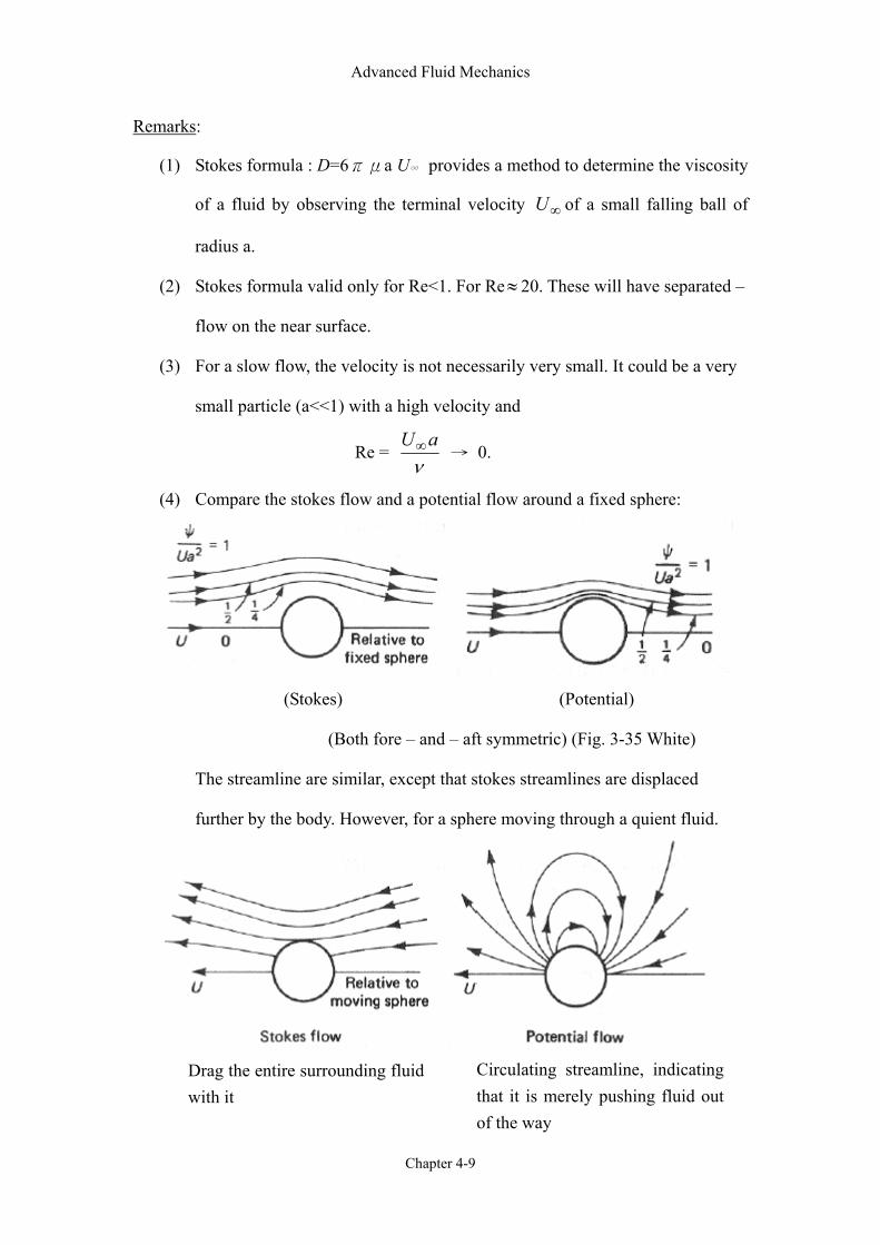
Advanced Fluid Mechanics
Chapter 4-9
Remarks:
(1) Stokes formula : D=6πμa U∞ provides a method to determine the viscosity
of a fluid by observing the terminal velocity ∞U of a small falling ball of
radius a.
(2) Stokes formula valid only for Re<1. For Re≈ 20. These will have separated –
flow on the near surface.
(3) For a slow flow, the velocity is not necessarily very small. It could be a very
small particle (a<<1) with a high velocity and
Re = ν
aU∞ → 0.
(4) Compare the stokes flow and a potential flow around a fixed sphere:
(Stokes) (Potential)
(Both fore – and – aft symmetric) (Fig. 3-35 White)
The streamline are similar, except that stokes streamlines are displaced
further by the body. However, for a sphere moving through a quient fluid.
Drag the entire surrounding fluid with it
Circulating streamline, indicating that it is merely pushing fluid out of the way
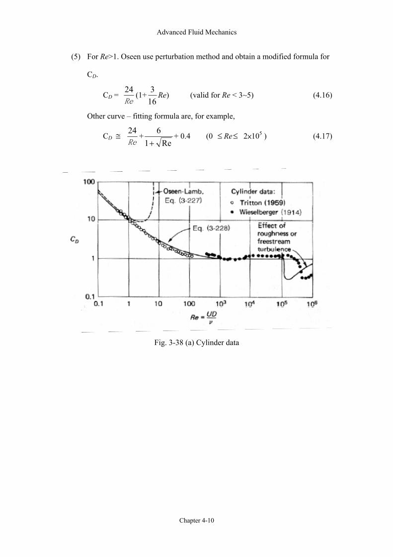
Advanced Fluid Mechanics
Chapter 4-10
(5) For Re>1. Oseen use perturbation method and obtain a modified formula for
CD.
CD = Re
24(1+
163
Re) (valid for Re < 3~5) (4.16)
Other curve – fitting formula are, for example,
CD ≅ Re
24+
Re16
++ 0.4 (0 ≤ Re≤ 2×10⁵ ) (4.17)
Fig. 3-38 (a) Cylinder data
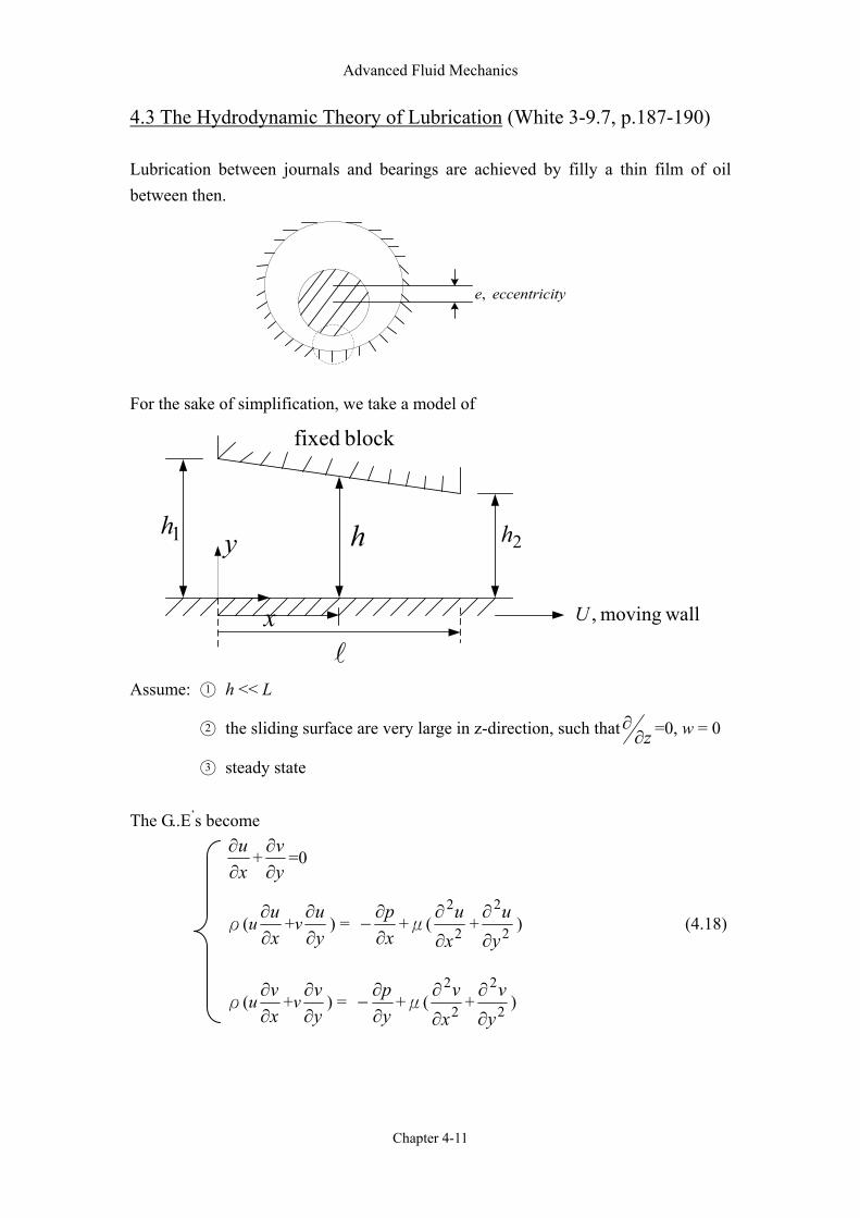
Advanced Fluid Mechanics
Chapter 4-11
4.3 The Hydrodynamic Theory of Lubrication (White 3-9.7, p.187-190) Lubrication between journals and bearings are achieved by filly a thin film of oil between then.
tyeccentricie ,
For the sake of simplification, we take a model of
y h1h2h
xl
block fixed
wallmoving ,U
Assume: 1 h << L
2 the sliding surface are very large in z-direction, such that z∂∂ =0, w = 0
3 steady state The G..E’s become
xu∂∂
+yv∂∂
=0
ρ(uxu∂∂
+vyu∂∂
) = xp∂∂
− +μ( 2
2
xu
∂
∂+ 2
2
yu
∂
∂) (4.18)
ρ(uxv∂∂
+vyv∂∂
) = yp∂∂
− +μ( 2
2
xv
∂
∂+ 2
2
yv
∂
∂)
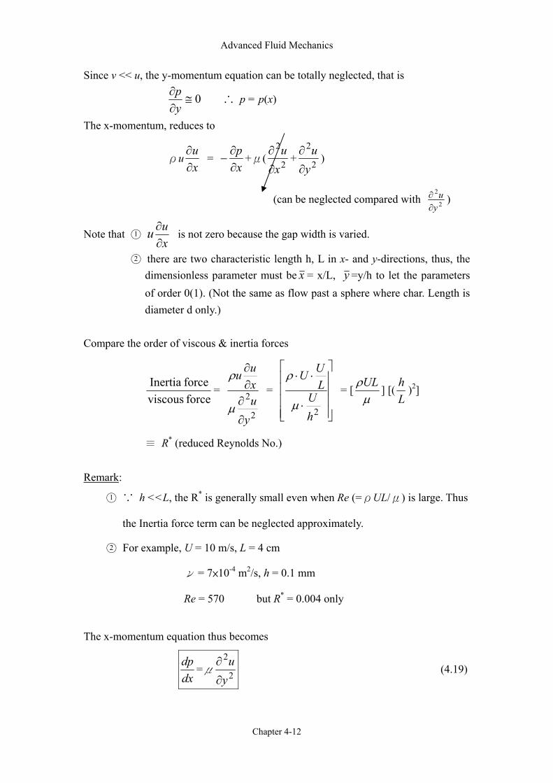
Advanced Fluid Mechanics
Chapter 4-12
Since v << u, the y-momentum equation can be totally neglected, that is
0≅∂∂
yp
∴ p = p(x)
The x-momentum, reduces to
ρuxu∂∂
= xp∂∂
− +μ( 2
2
xu
∂
∂+ 2
2
yu
∂
∂)
(can be neglected compared with 2
2
yu
∂∂ )
Note that 1 uxu∂∂ is not zero because the gap width is varied.
2 there are two characteristic length h, L in x- and y-directions, thus, the dimensionless parameter must be x = x/L, y =y/h to let the parameters of order 0(1). (Not the same as flow past a sphere where char. Length is diameter d only.)
Compare the order of viscous & inertia forces
force viscousforce Inertia
=
2
2
yuxuu
∂
∂∂∂
µ
ρ =
⋅
⋅⋅
2hU
LUU
µ
ρ = [
µρUL
] [(Lh
)2]
≡ R* (reduced Reynolds No.) Remark:
1 ∵ h <<L, the R* is generally small even when Re (=ρUL/μ) is large. Thus
the Inertia force term can be neglected approximately.
2 For example, U = 10 m/s, L = 4 cm
ν = 7×10⁻⁴ m2/s, h = 0.1 mm
Re = 570 but R* = 0.004 only
The x-momentum equation thus becomes
dxdp
=μ 2
2
yu
∂
∂ (4.19)

Advanced Fluid Mechanics
Chapter 4-13
B.C’s: 1 y =0, u =U 2 y =h, u = 0 3 x = 0, p = p0 4 x = L, p = p0
Note that dp/dx here is no longer constant (such as the couette flow between two
parallel walls), it must satisfy the pressure P0 at both ends. The dp/dx must be
determined in such a way as to satisfy the continuity equation in every section of the
form
Q = ∫ (udy + vdx) = ∫)(
0xh
udy = const (4.20)
The solution of Eq. (4.19) with given B.C’s is
u = U(1-hy
) - )1()(2
2
hy
hy
dxdph
−µ
(4.21)
Here, dp/dx is determined by sub. (4.21) into (4.20), as
Q = 2
Uh- )(
12
3
dxdph
µ
Or
dxdp
= 12μ( 22hU
- 3hQ
) (4.22)
integrate with B.C (p = p0 at x=0 ), we have
p = p0 + 6μU ∫x
hdx
0 2 -12μQ ∫x
hdx
0 3 (4.23)
≡ b1(x) ≡ b2(x)
Inserting B.C of p =p0 at x = L, we get
Q = 21
U)()(
2
1LbLb
= 21
UH (4.24)
≡ characteristic thickness ≡H
This is an assumed assumption for the model. For a certain segment in lubrication fluid, the pressure is not the same on both ends

Advanced Fluid Mechanics
Chapter 4-14
We may conclude the procedure of solution as follows:
(1) Known wedge shape h(x)
(2) Obtain b1(L) & b2(L), as well as H & Q
(3) The pressure distribution (4.23) can be rewritten as
p(x) = p0 + 6μUb1(x) -12μQb2(x) (4.25)
and is readily obtained.
(4) The dp/dx, Eq. (4.22) can be written and calculated as
dxdp
= 26h
Uµ(1-
hH
) (4.26)
(5) Knowing dp/dx, the velocity distribution can be found from Eq. (4.21)
Remark:
(1) pmax or pmin occurs where h =H.
(2) For a straight wedge with h1 & h2 at both ends, we get
p(x) = p0 + 6μU 221
22
21
))((h
hhhhhh
L −−
−
21
0
/ hULpp
µ−
1
2
3
0 5.0 1
8.0
7.0
5.0
4.0
3.01
2 =hh
exit. near the occurs andhigher become
pressuremax thedecrease as 1
2h
h
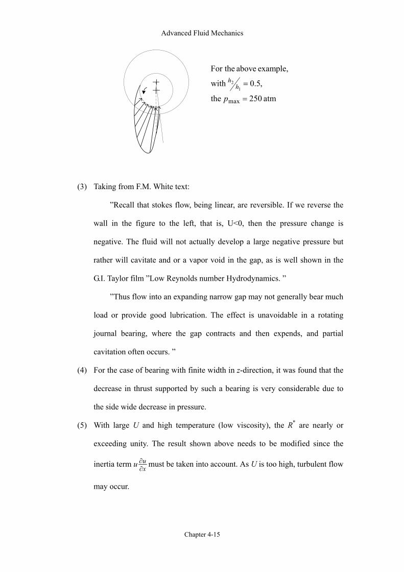
Advanced Fluid Mechanics
Chapter 4-15
atm 250 the
,5.0with
example, above For the
max
12
=
=
ph
h
(3) Taking from F.M. White text:
”Recall that stokes flow, being linear, are reversible. If we reverse the
wall in the figure to the left, that is, U<0, then the pressure change is
negative. The fluid will not actually develop a large negative pressure but
rather will cavitate and or a vapor void in the gap, as is well shown in the
G.I. Taylor film ”Low Reynolds number Hydrodynamics. ”
”Thus flow into an expanding narrow gap may not generally bear much
load or provide good lubrication. The effect is unavoidable in a rotating
journal bearing, where the gap contracts and then expends, and partial
cavitation often occurs. ”
(4) For the case of bearing with finite width in z-direction, it was found that the
decrease in thrust supported by such a bearing is very considerable due to
the side wide decrease in pressure.
(5) With large U and high temperature (low viscosity), the R* are nearly or
exceeding unity. The result shown above needs to be modified since the
inertia term u xu∂∂ must be taken into account. As U is too high, turbulent flow
may occur.
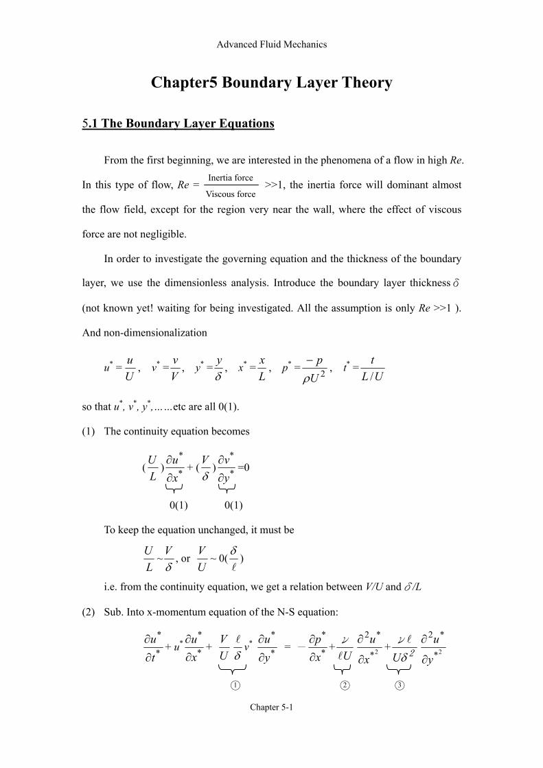
Advanced Fluid Mechanics
Chapter 5-1
Chapter5 Boundary Layer Theory 5.1 The Boundary Layer Equations
From the first beginning, we are interested in the phenomena of a flow in high Re.
In this type of flow, Re = >>1, the inertia force will dominant almost
the flow field, except for the region very near the wall, where the effect of viscous
force are not negligible.
In order to investigate the governing equation and the thickness of the boundary
layer, we use the dimensionless analysis. Introduce the boundary layer thicknessδ
(not known yet! waiting for being investigated. All the assumption is only Re >>1 ).
And non-dimensionalization
u* =Uu
, v* =Vv
, y* =δy
, x* =Lx
, p* = 2Up
ρ−
, t* =UL
t/
so that u*, v*, y*,……etc are all 0(1).
(1) The continuity equation becomes
(LU
) *
*
xu∂∂
+ (δV
) *
*
yv∂∂
=0
0(1) 0(1)
To keep the equation unchanged, it must be
LU
~δV
, or UV
~ 0(l
δ)
i.e. from the continuity equation, we get a relation between V/U andδ/L
(2) Sub. Into x-momentum equation of the N-S equation:
*
*
tu∂
∂+ u*
*
*
xu∂∂
+ UV
δl
v* *
*
yu∂
∂ = - *
*
xp∂∂
+Ulν
2*
*2
x
u
∂
∂+
2
ν
δUl
2*
*2
y
u
∂
∂
1 2 3
Inertia force
Viscous force

Advanced Fluid Mechanics
Chapter 5-2
all the '' * '' terms are 0(1), we need only to consider the 3 coefficients above.
1 = UV
δl
~ 0(1) from continuity equation
2 = Ulν
= Re
1 → 0 (∵ Re >>1), therefore, this term can be dropped out
compared with other)
3 2
ν
δUl
= ? In order to keep this term (otherwise, all the viscous term
disappear, it becomes the inviscid flow. This is the flow outside the boundary
layer, not what we want.) It should be also order of 1. So
2
ν
δUl
~ 0(1) → δ~Ulν
~U
xν
that is from dimensionless analysis, we already have a ideal about the
boundary layer thickness.
δ~U
xν
(3) Sub. Into y-momentum equation, we have
*
*
tv∂
∂+ u*
*
*
xv∂
∂+ (
UV
)(δl
)v* *
*
yv∂
∂= -
VU
δl
*
*
yp∂
∂+
Ulν
2*
*2
x
u
∂
∂+
2
ν
δUl
2*
*2
y
u
∂
∂
1 2 3 4
where 1 = UV
δl
~ 0(1) (continuity equation) (o.k.)
3 = Ulν
= Re
1 → 0 (∵ Re >>1) can be neglected
4 2
ν
δUl
= Re
1(δl
)2 ~ 0(1) from the result of x-momentum equation
2 -VU
δl
>> 0(1) , so that we can see that this term are larger than
other terms, the y-momentum equation can be written contained only
dominant term as yp∂
∂ = 0

Advanced Fluid Mechanics
Chapter 5-3
i.e. we can conclude p = p(x) only.
So we conclude:
For a flow with Re >>1, the flow very near the wall is governed by the equation
(incompressible flow)
xu∂∂
+yv∂∂
= 0 (5.1)
tu∂∂
+ uxu∂∂
+ vyu∂∂
= -ρ1
dxdp
+ν 2
2
yu
∂
∂
and yp∂∂
= 0. This equation is called”boundary layer equation”
Remark:
Compare the Navier-stokes equation and the boundary layer equation, and explain
why the latter is easier to be solved numerically?
(Ans:) For simplicity, let’s consider the incompressible flow as an example:
Navier-stokes equation:
xu∂∂
+yv∂∂
= 0
tu∂∂
+ uxu∂∂
+ vyu∂∂
= -ρ1
dxdp
+ν( 2
2
2
2
yu
xu
∂
∂+
∂
∂)
tv∂∂
+ uxv∂∂
+ vyv∂∂
= -ρ1
yp∂∂
+ν( 2
2
2
2
yv
xv
∂
∂+
∂
∂)
Boundary layer equation:
xu∂∂
+yv∂∂
=0
tu∂∂
+ uxu∂∂
+ vyu∂∂
= -ρ1
xp∂∂
+ν 2
2
yu
∂
∂
yp∂
∂ = 0
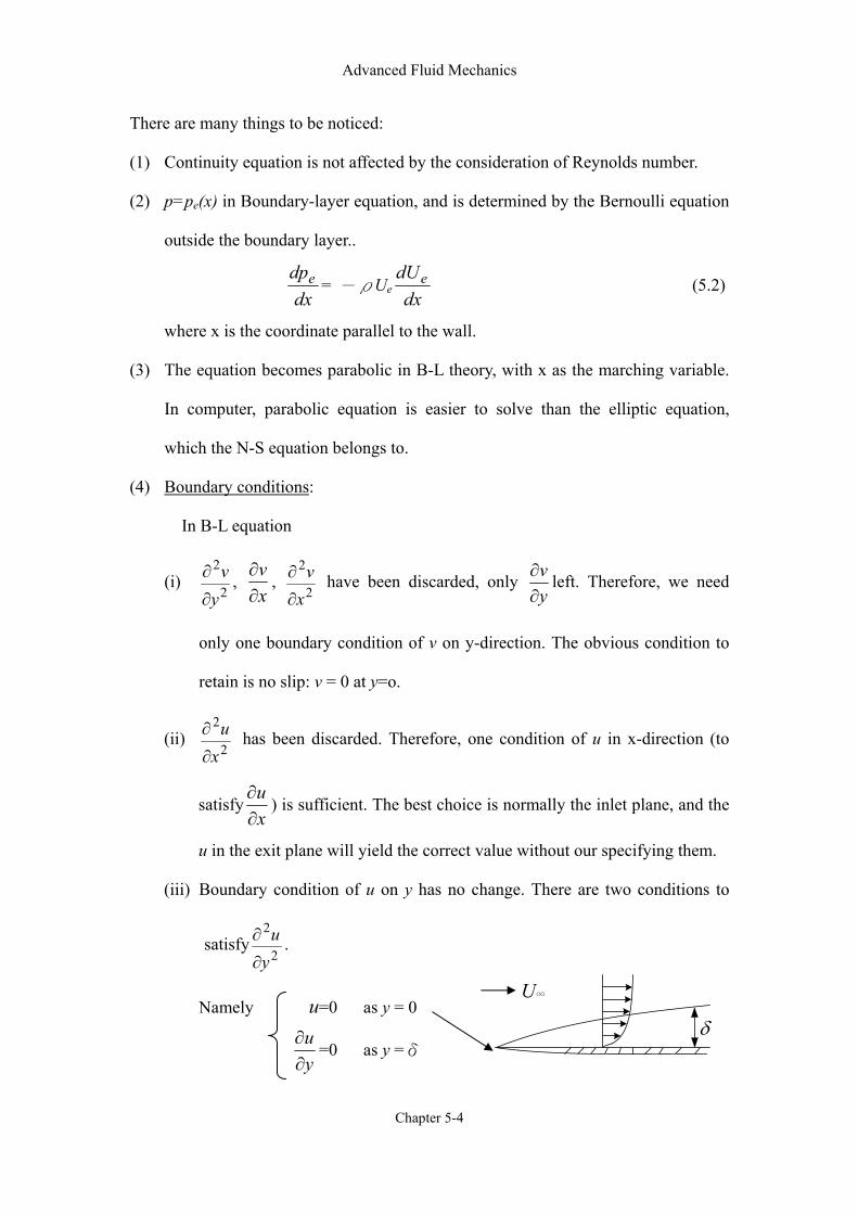
Advanced Fluid Mechanics
Chapter 5-4
δ
There are many things to be noticed:
(1) Continuity equation is not affected by the consideration of Reynolds number.
(2) p=pe(x) in Boundary-layer equation, and is determined by the Bernoulli equation
outside the boundary layer..
dxdpe = -ρUe
dxdUe (5.2)
where x is the coordinate parallel to the wall.
(3) The equation becomes parabolic in B-L theory, with x as the marching variable.
In computer, parabolic equation is easier to solve than the elliptic equation,
which the N-S equation belongs to.
(4) Boundary conditions:
In B-L equation
(i) 2
2
yv
∂
∂ , xv∂∂
, 2
2
xv
∂
∂ have been discarded, only yv∂∂ left. Therefore, we need
only one boundary condition of v on y-direction. The obvious condition to
retain is no slip: v = 0 at y=o.
(ii) 2
2
xu
∂
∂ has been discarded. Therefore, one condition of u in x-direction (to
satisfyxu∂∂
) is sufficient. The best choice is normally the inlet plane, and the
u in the exit plane will yield the correct value without our specifying them.
(iii) Boundary condition of u on y has no change. There are two conditions to
satisfy2
2
yu
∂
∂ .
Namely u=0 as y = 0
yu∂∂
=0 as y =δ
U∞
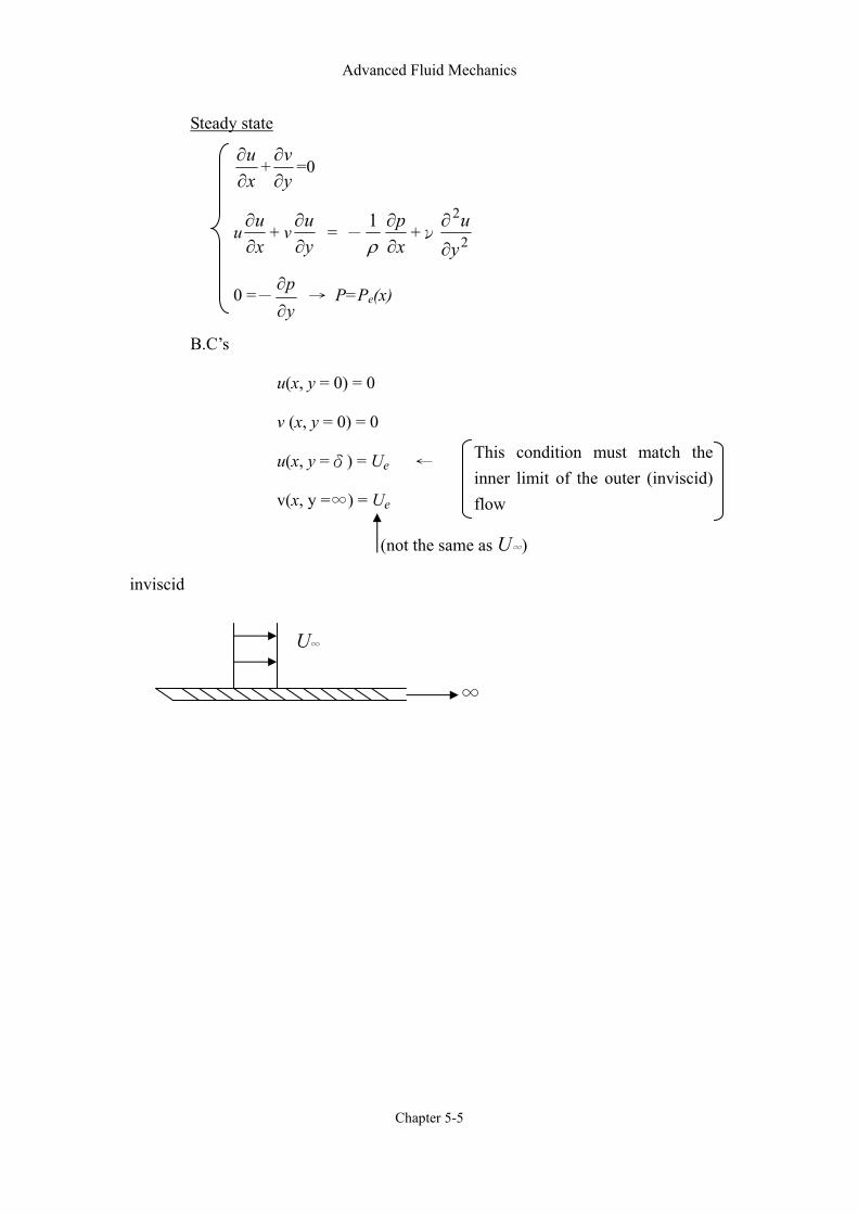
Advanced Fluid Mechanics
Chapter 5-5
Steady state
xu∂∂
+yv∂∂
=0
uxu∂∂
+ vyu∂∂
= -ρ1
xp∂∂
+ν 2
2
yu
∂
∂
0 =-yp∂
∂ → P=Pe(x)
B.C’s
u(x, y = 0) = 0
v (x, y = 0) = 0
u(x, y =δ) = Ue ←
v(x, y =∞) = Ue
(not the same as U∞)
inviscid
U∞
∞
This condition must match the inner limit of the outer (inviscid) flow
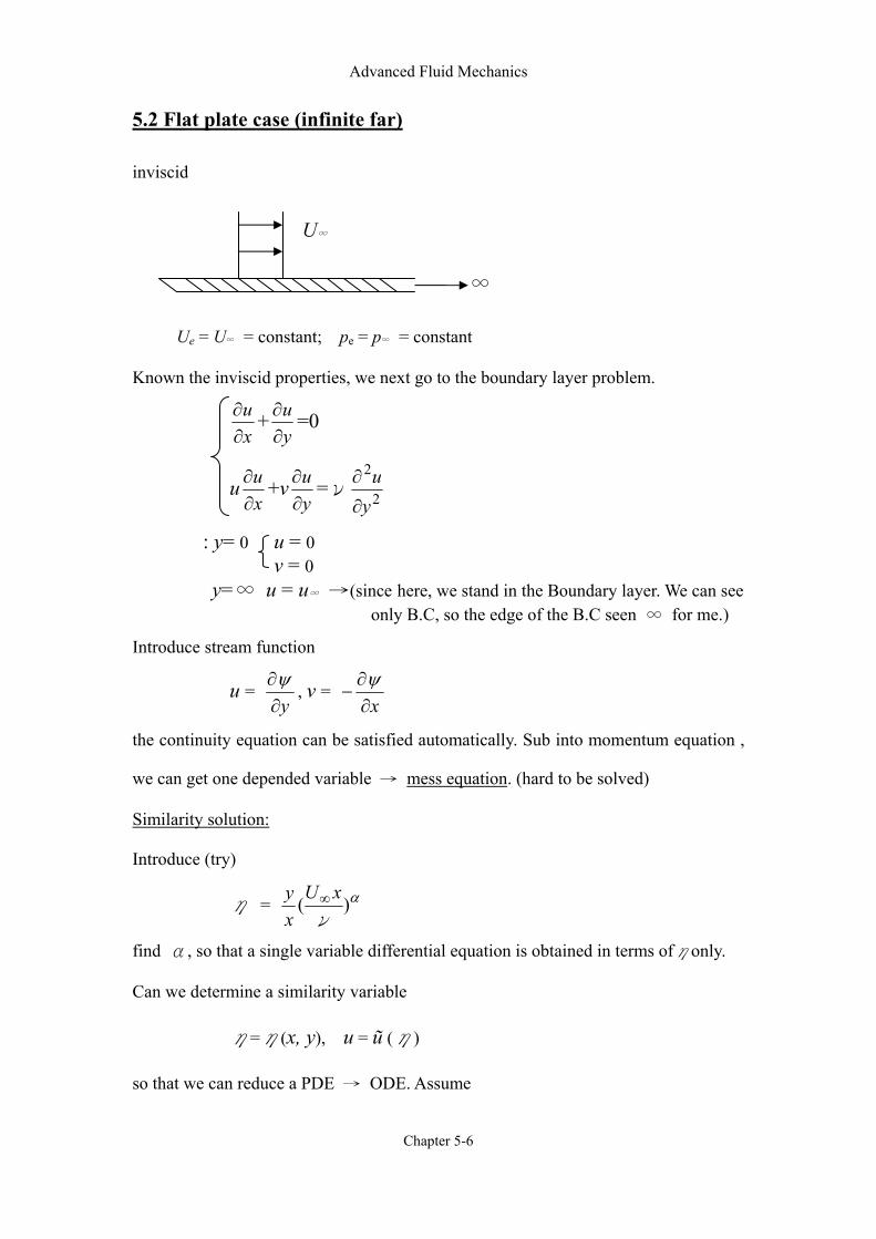
Advanced Fluid Mechanics
Chapter 5-6
5.2 Flat plate case (infinite far) inviscid
Ue = U∞ = constant; pe = p∞ = constant
Known the inviscid properties, we next go to the boundary layer problem.
xu∂∂ +
yu∂∂ =0
uxu∂∂ +v
yu∂∂ =ν 2
2
yu
∂
∂
: y= 0 u = 0 v = 0
y=∞ u = u∞ →(since here, we stand in the Boundary layer. We can see only B.C, so the edge of the B.C seen ∞ for me.)
Introduce stream function
u = y∂
∂ψ, v =
x∂∂
−ψ
the continuity equation can be satisfied automatically. Sub into momentum equation ,
we can get one depended variable → mess equation. (hard to be solved)
Similarity solution:
Introduce (try)
η = α)(ν
xUxy ∞
find α, so that a single variable differential equation is obtained in terms ofηonly.
Can we determine a similarity variable
η=η(x, y), u = ũ (η)
so that we can reduce a PDE → ODE. Assume
U∞
∞

Advanced Fluid Mechanics
Chapter 5-7
0=ψ
η= α)(ν
xUxy ∞ → α=1/2
Dimension of length: x, y, ∞U
ν
Dimensionless of length: ỹ =∞U
yν
= ν
yU∞ , x~ = ν
xU∞
∞UU
= fn(η) = 'f (η)
y∂∂ψ
=U∞'f (η)
y∂∂
∂∂ ηηψ
=U∞'f (η)
µψ∂∂
(ν∞U
)1/2
21
1x
= U∞'f (η)
µψ∂∂
= U∞(∞U
ν )1/2 x1/2 'f (η)
ψ = U∞(∞U
ν )1/2 x1/2 f (η) + const
∴ η= α)(ν
xUxy ∞
ψ = U∞(∞U
ν )1/2 x1/2 f (η)
u =y∂
∂ψ=U∞
'f (η)
v =x∂
∂−
ψ= -U∞(
∞Uν )1/2
2
12
1x
f (η) + x1/2
∂∂
xddf ηη
x∂∂η = (
∞Uν )1/2
−
212
1xy
x=
x2η
−
v = -U∞(∞U
ν )1/2
−
21
21
22
'
xf
xf η
anticipate f (η) as a dimensionless stream
function.
η=0 so thatψ =0 represent the body shape(∵along body (y=0)→η=0, but f(0)=0 from B.C.)
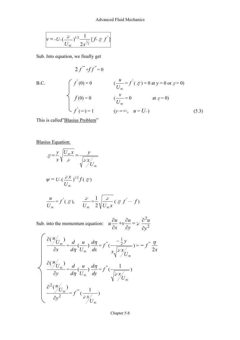
Advanced Fluid Mechanics
Chapter 5-8
v = -U∞(∞U
ν )1/2
21
21x
[ f-η 'f ]
Sub. Into equation, we finally get
2 '''f +f ''f = 0
B.C. 'f (0) = 0 (∞U
u= 'f (η) = 0 at y = 0 orη= 0)
f (0) = 0 (∞U
v= 0 atη= 0)
'f (∞) = 1 (y→∞, u = U∞) (5.3)
This is called”Blasius Problem”
Blasius Equation:
η=ν
xUxy ∞ =
∞Uxy
ν
ψ = U∞(∞Uxν )1/2 f (η)
∞Uu
= 'f (η), ∞U
ν=
xU∞
ν
21
(η 'f - f )
Sub. into the momentum equation: uxu∂∂ +v
yu∂∂ =ν 2
2
yu
∂
∂
xU
u
∂
∂∞
)(= )(
∞Uu
ddη dx
dη= ''f (
∞
−
Uxx
y
ν21
) = - ''fx2η
yU
u
∂
∂∞
)(= )(
∞Uu
ddη dy
dη= ''f (
∞Uxν
1)
2
2 )(
yU
u
∂
∂∞ = '''f (
∞Uxν1
)
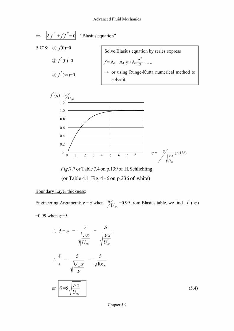
Advanced Fluid Mechanics
Chapter 5-9
⇒ 2 '''f + f ''f = 0 ”Blasius equation”
B.C’S: 1 f(0)=0
2 'f (0)=0
3 'f (∞)=0
0
2.0
4.0
6.0
8.0
0.1
2.1∞
= Uuf )(' η
1 2 3 4 5 6 70
∞
=
Ux
yν
η )136.( p
gSchlichtin H. of p.139on 7.4 Tableor 7.7.Fig
white)of p.236on 6-4 Fig. 4.1 Table(or
8
Boundary Layer thickness:
Engineering Argumemt: y =δwhen ∞U
u =0.99 from Blasius table, we find 'f (η)
=0.99 whenη=5.
∴ 5 =η =
∞Ux
yν
=
∞Uxν
δ
∴xδ
=
ν
xU∞
5 =
xRe5
or δ=5∞Uxν
(5.4)
Solve Blasius equation by series express
f = A0 +A1η+A2 2
2η +….
→ or using Runge-Kutta numerical method to solve it.
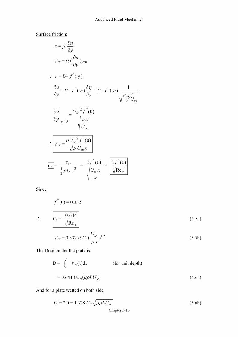
Advanced Fluid Mechanics
Chapter 5-10
Surface friction:
τ=μyu∂∂
τw =μ(yu∂∂ )y=0
∵ u = U∞'f (η)
yu∂∂
= U∞''f (η)
y∂∂η
= U∞''f (η)
∞Uνx
1
0=∂
∂
yyu
=
∞
∞
Ux
fUν
)0(''2
∴τw =xU
fU
∞
∞
ν
)0(''2µ
Cf = 221
∞Uw
ρτ
=
ν
xUf
∞
)0(2 '' =
x
fRe
)0(2 ''
Since
''f (0) = 0.332
∴ Cf = xRe
644.0 (5.5a)
τw = 0.332μU∞(x
Uν
∞ )1/2 (5.5b)
The Drag on the flat plate is
D = ∫L0
τw(x)dx (for unit depth)
= 0.644 U∞ ∞LUµρ (5.6a)
And for a plate wetted on both side
'D = 2D = 1.328 U∞ ∞LUµρ (5.6b)
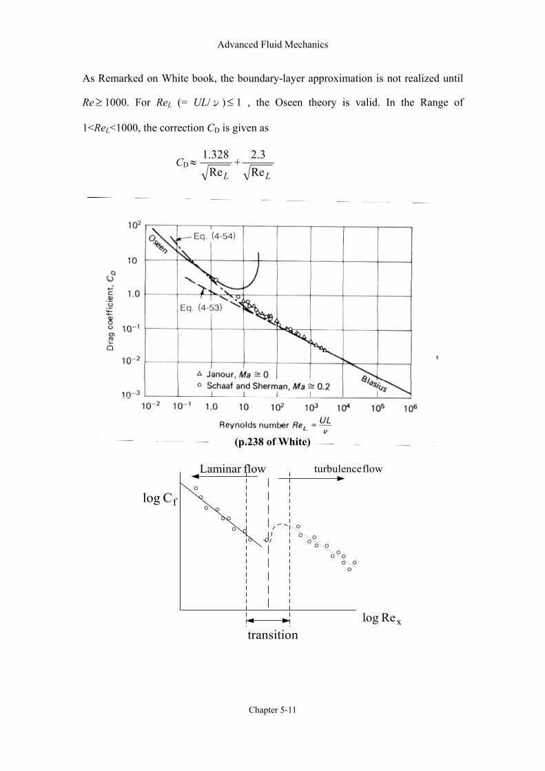
Advanced Fluid Mechanics
Chapter 5-11
As Remarked on White book, the boundary-layer approximation is not realized until
Re≥ 1000. For ReL (= UL/ν)≤ 1 , the Oseen theory is valid. In the Range of
1<ReL<1000, the correction CD is given as
CD≈LRe
328.1+
LRe3.2
oo
o oooo o
o oo
ooo ooooooo
o
fC log
xRe log
flow turbulence
transition
flowLaminar
(p.238 of White)
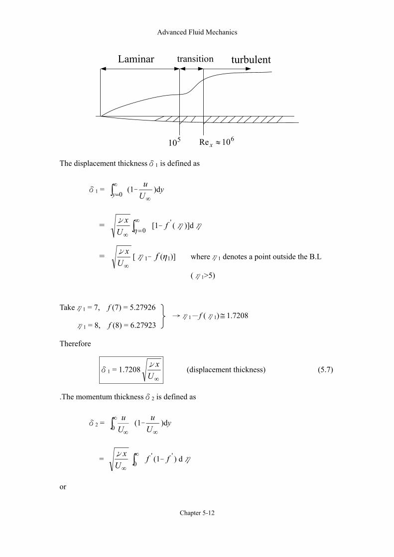
Advanced Fluid Mechanics
Chapter 5-12
510 610Re ≈x
Laminar transition turbulent
The displacement thicknessδ1 is defined as
δ1 = ∫∞
=0y(1-
∞Uu
)dy
= ∫∞
=∞
0ηUxν
[1- 'f (η)]dη
= ∞Uxν
[η1- f (η1)] whereη1 denotes a point outside the B.L
(η1>5)
Takeη1 = 7, f (7) = 5.27926
η1 = 8, f (8) = 6.27923
Therefore
δ1 = 1.7208∞Uxν
(displacement thickness) (5.7)
.The momentum thicknessδ2 is defined as
δ2 = ∫∞
∞0 U
u (1-
∞Uu
)dy
= ∞Uxν∫∞
0'f (1- 'f ) dη
or
→η1-f (η1)≅ 1.7208
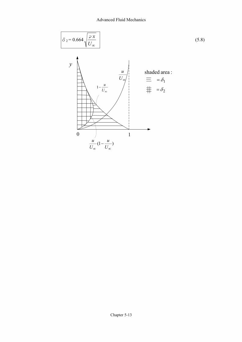
Advanced Fluid Mechanics
Chapter 5-13
δ2 = 0.664∞Uxν
(5.8)
0 1
y
∞−
Uu1
)1(∞∞
−U
uU
u
∞Uu :area shaded
1δ=
2δ=
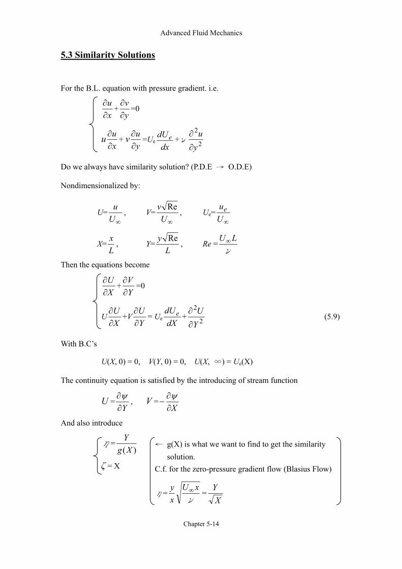
Advanced Fluid Mechanics
Chapter 5-14
5.3 Similarity Solutions
For the B.L. equation with pressure gradient. i.e.
xu∂∂
+yv∂∂
=0
uxu∂∂
+ vyu∂∂
=Uedx
dUe +ν 2
2
yu
∂
∂
Do we always have similarity solution? (P.D.E → O.D.E)
Nondimensionalized by:
U=∞U
u, V=
∞Uv Re
, Ue=∞U
ue
X=Lx
, Y=L
y Re, Re =
ν
LU∞
Then the equations become
XU∂∂
+YV∂∂
=0
UXU∂∂
+VYU∂∂
= UedX
dUe + 2
2
YU
∂
∂ (5.9)
With B.C’s
U(X, 0) = 0, V(Y, 0) = 0, U(X, ∞) = Ue(X)
The continuity equation is satisfied by the introducing of stream function
U =Y∂
∂ψ, V =
X∂∂
−ψ
And also introduce
η=)(Xg
Y
ζ = X
← g(X) is what we want to find to get the similarity solution.
C.f. for the zero-pressure gradient flow (Blasius Flow)
η=ν
xUxy ∞ =
XY
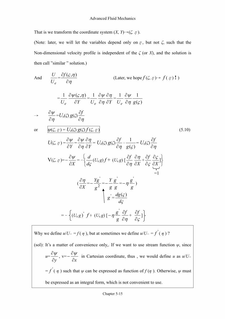
Advanced Fluid Mechanics
Chapter 5-15
That is we transform the coordinate system (X, Y)→(ζ,η).
(Note: later, we will let the variables depend only onη, but not ζ, such that the
Non-dimensional velocity profile is independent of the ζ (or X), and the solution is
then call ”similar ” solution.)
And eU
U=
ηης
∂∂ ),(f
(Later, we hope f (ζ,η)→ f (η) ! )
=eU
1Y∂
∂ ),( ηςψ=
eU1
Y∂∂
∂∂ ηηψ
=eU
1)(
1ςη
ψg∂
∂
→ ηψ∂∂
=Ue(ζ) g(ζ)η∂∂f
or ψ(ζ,η) = Ue(ζ) g(ζ) f (ζ,η) (5.10)
U(ζ,η) =Y∂
∂ψ=
Y∂∂
∂∂ ηηψ
= Ue(ζ) g(ζ)η∂∂f
)(1ςg
⋅ = Ue(ζ)η∂∂f
V(ζ,η)=X∂∂
−ψ
= -ςd
d(Ue g) f + (Ue g) [
η∂∂f
X∂∂η
+ς∂∂f
∂∂ ]Xς
=1
(X∂∂η
= 2
'
gYg
− =gg
gY '
− =gg '
η− )
'g =ςς
ddg )(
= - (Ue g ') f + (Ue g) [gg '
η−η∂∂f
+ ς∂∂f
]
Why we define u/U∞ = f ( η ), but at sometimes we define u/U∞ = 'f ( η ) ?
(sol): It’s a matter of convenience only,. If we want to use stream function ψ, since
u=y∂
∂ψ, v=
x∂∂
−ψ
in Cartesian coordinate, thus , we would define u as u/U∞
= 'f ( η ) such that ψ can be expressed as function of f (η ). Otherwise, ψ must
be expressed as an integral form, which is not convenient to use.
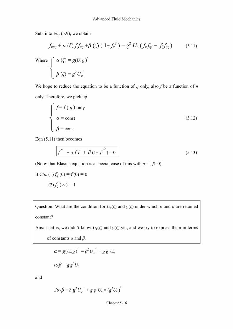
Advanced Fluid Mechanics
Chapter 5-16
Sub. into Eq. (5.9), we obtain
fηηη + α (ζ) f fηη +β (ζ) ( 1- fη2 ) = g2 Ue ( fη fηζ - fζ fηη ) (5.11)
Where α (ζ) = g(Ue g ')
β (ζ) = g2 'eU
We hope to reduce the equation to be a function of η only, also f be a function of η
only. Therefore, we pick up
f = f ( η ) only
α = const (5.12)
β = const
Eqn (5.11) then becomes
'''f + α f ''f + β (1-2'f ) = 0 (5.13)
(Note: that Blasius equation is a special case of this with α=1, β=0)
B.C’s: (1) fη (0) = f (0) = 0
(2) fη (∞) = 1
Question: What are the condition for Ue(ζ) and g(ζ) under which α and β are retained
constant?
Ans: That is, we didn’t know Ue(ζ) and g(ζ) yet, and we try to express them in terms
of constants α and β.
α = g(Ue g ') = g2 'eU + g 'g Ue
α-β = g 'g Ue
and
2α-β =2 g2 'eU + g 'g Ue = (g2Ue
')
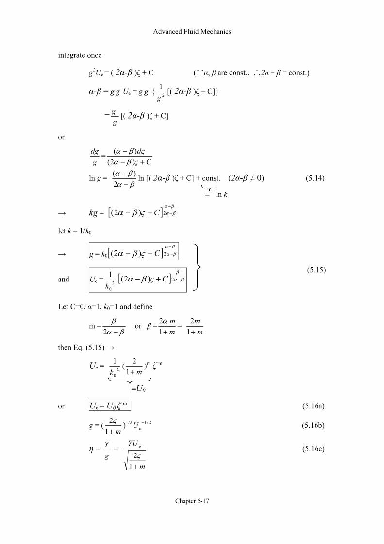
Advanced Fluid Mechanics
Chapter 5-17
integrate once
g2Ue = ( 2α-β )ζ + C (∵α, β are const., ∴2α - β = const.)
α-β = g 'g Ue = g 'g 2
1g
[( 2α-β )ζ + C]
=gg '
[( 2α-β )ζ + C]
or
gdg =
Cd+−
−ςβαςβα
)2()(
ln g = βαβα−−
2)( ln [( 2α-β )ζ + C] + const. (2α-β ≠ 0) (5.14)
≡ −ln k
→ kg = [ ] βαβα
ςβα −−
+− 2)2( C
let k = 1/k0
→ g = k0 [ ] βαβα
ςβα −−
+− 2)2( C
and Ue = 20
1k
[ ] βαβ
ςβα −+− 2)2( C
Let C=0, α=1, k0=1 and define
m =βα
β−2
or β =mm
+1 2α =
mm+12
then Eq. (5.15) →
Ue = 20
1k
(m+1
2 )m ζ m
≡U0
or Ue = U0 ζ m (5.16a)
g = (m+1
2ς )1/2 2/1−eU (5.16b)
η = gY
=
m
YU e
+12ς
(5.16c)
(5.15)

Advanced Fluid Mechanics
Chapter 5-18
1 2 3 4 5
2.0
4.0
6.0
8.0
0.1
)(' ηfU
u=
∞
yx
Umν2
1+=η
091.0−0654.0−
014=m
separation
This is called the” Falkner-Skan Problem”. From potential flow theory, the Eq. (5.16b)
is corresponding to an inviscid flow passing a wedge of angle πβ.
πβ or 2πβ
force.)gravity no plane, ( yx −
Special cases:
(1) For m = 1 → β = 1, stagnation flow
(2) For m = 0 → β = 0, flat plate at zero incidence.
The solution of Eq.(5.13) namely
'''f + ''ff + β(1-2'f ) = 0
with f(0) = 'f (0) = 0, 'f (1) = 1 is
m πβ → β
-0.091 -0.199π -35.8 -0.199
-0.0654 -0.14π -25.2 -0.14
0 0 0 0
1 π 180
4 1.6π 288
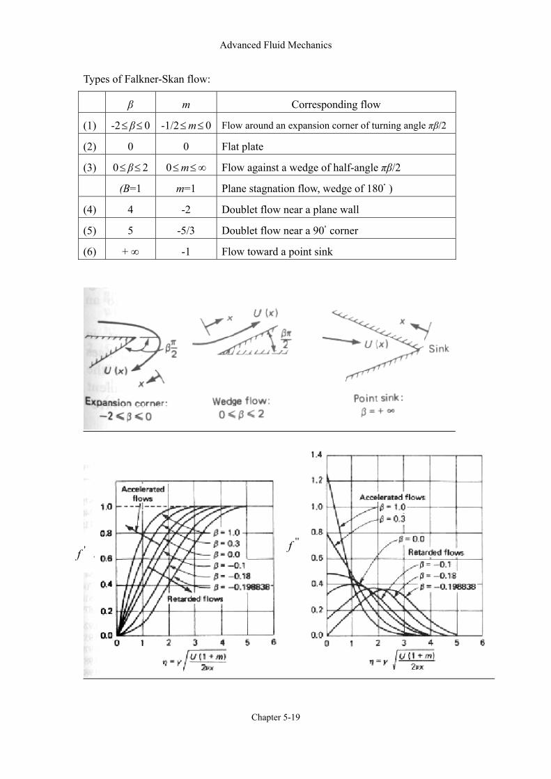
Advanced Fluid Mechanics
Chapter 5-19
Types of Falkner-Skan flow:
β m Corresponding flow
(1) -2≤ β≤ 0 -1/2≤m≤ 0 Flow around an expansion corner of turning angle πβ/2
(2) 0 0 Flat plate
(3) 0≤ β≤ 2 0≤m≤∞ Flow against a wedge of half-angle πβ/2
(Β=1 m=1 Plane stagnation flow, wedge of 180 )
(4) 4 -2 Doublet flow near a plane wall
(5) 5 -5/3 Doublet flow near a 90 corner
(6) + ∞ -1 Flow toward a point sink
'f ''f

Advanced Fluid Mechanics
Chapter 5-20
Note:
(1) For incompressible wedge flow. As the inclined angle πβ/2 increased, the
fluid is accelerated, and the boundary layer becomes thinner. However, the
τw is increased.
Remark:
(1) From f ’ ~ η figure, we can see that boundary layer grows thicker & thicker
as β decreasing. (For β = -0.199, separation occurs at y=0.)
(2) From ''f ~ η figure:
''f corresponding to shearing stress. For β>0, the shearing stress
decreases as η increases. However, as β < 0, the ''f rises and they decrease as
η increases. This is because
dxdpe = µ
02
2
=∂∂
yyu =
wally∂∂ τ
Thus for β < 0 (decelerating flow,dxdpe > 0). The
wally∂∂ τ > 0, therefore,
''f will rise near wall as η increases.
(3) From ''f ~ η figure:
-0.199 ≤ β ≤ 0 ← there are (at least) two solution
β < -0.199 ←multiple solution
(See F.M. White. P.245 for detail)
(4) As the N-S equations are no unique, the B.L. equations also show multiple
solutions.
(5) As described in Dr. Sepri’s Note, the conditions leading to a similar solution
are:
(i) B.C need to be similar → (ρv)0 restricted in form
(ii) I.C is similar, that is, can’t accept an arbitrary f0(η)
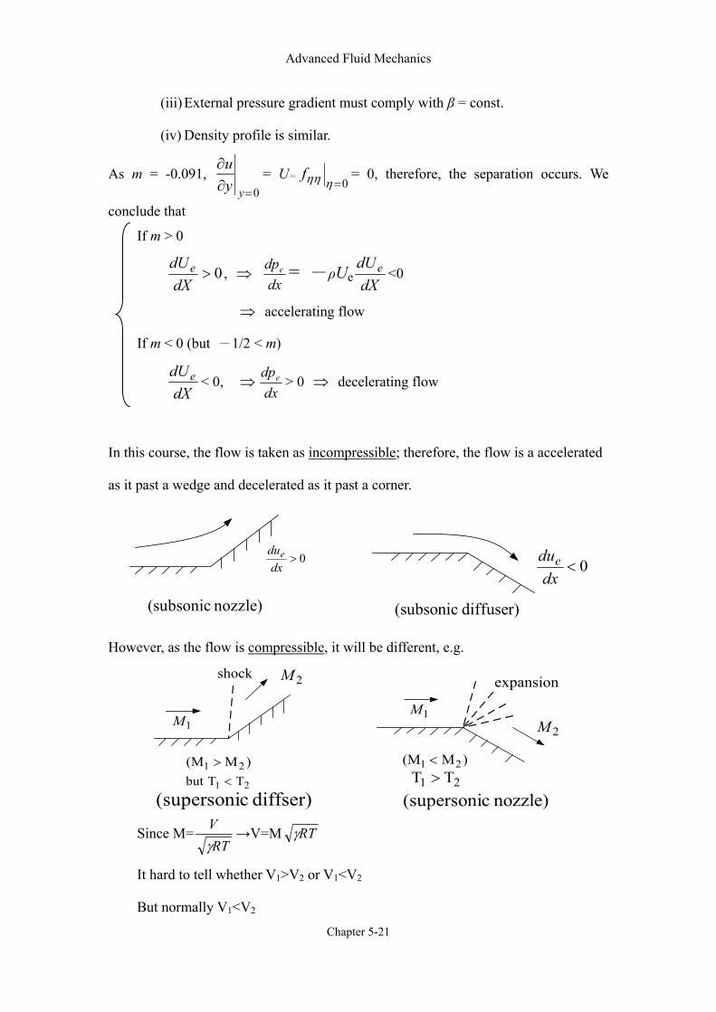
Advanced Fluid Mechanics
Chapter 5-21
(iii) External pressure gradient must comply with β = const.
(iv) Density profile is similar.
As m = -0.091, 0=∂
∂
yyu
= U∞0=ηηηf = 0, therefore, the separation occurs. We
conclude that
If m > 0
0>dX
dUe , ⇒ dxdpe = -ρUe dX
dUe <0
⇒ accelerating flow
If m < 0 (but -1/2 < m)
dX
dUe < 0, ⇒dxdpe > 0 ⇒ decelerating flow
In this course, the flow is taken as incompressible; therefore, the flow is a accelerated
as it past a wedge and decelerated as it past a corner.
0>dx
due
nozzle) (subsonic
0<dx
due
diffuser) (subsonic
However, as the flow is compressible, it will be different, e.g.
1M
2Mshock
)M(M 21 >
expansion
1M2M
)M(M 21 <
21 TT >21 TTbut <
diffser) c(supersoni nozzle) c(supersoni
Since M=RT
Vγ
→V=M RTγ
It hard to tell whether V1>V2 or V1<V2
But normally V1<V2

Advanced Fluid Mechanics
Chapter 5-22
(In x-y plane, no gravity force acting)
0>m0<m
.0→u
.
∞→u
)(X
)(V
∞U
0>dx
dUe 0<dx
dUe
seperation ,00=
∂∂
=yyu
eU
12
3 45. .
For curve 1-4, 2-4 & 3-4, the velocity profile at 5 will not be the same.
(Cannot determine thedx
dUe >0 ordx
dUe <0 from the
slope of the local surface w.r.t the free-stream direction.
It normally further upstream as shown)
Advanced Fluid Mechanics
Chapter 5-23
Problem:
Show that (δ*/τw) dp/dx represents the ratio of pressure force to wall friction force
in the fluid in a boundary layer. Show that it is constant for any of the Falkner-Skan
wedge flows. (J. schetz. P. 92, prob. 4.6)
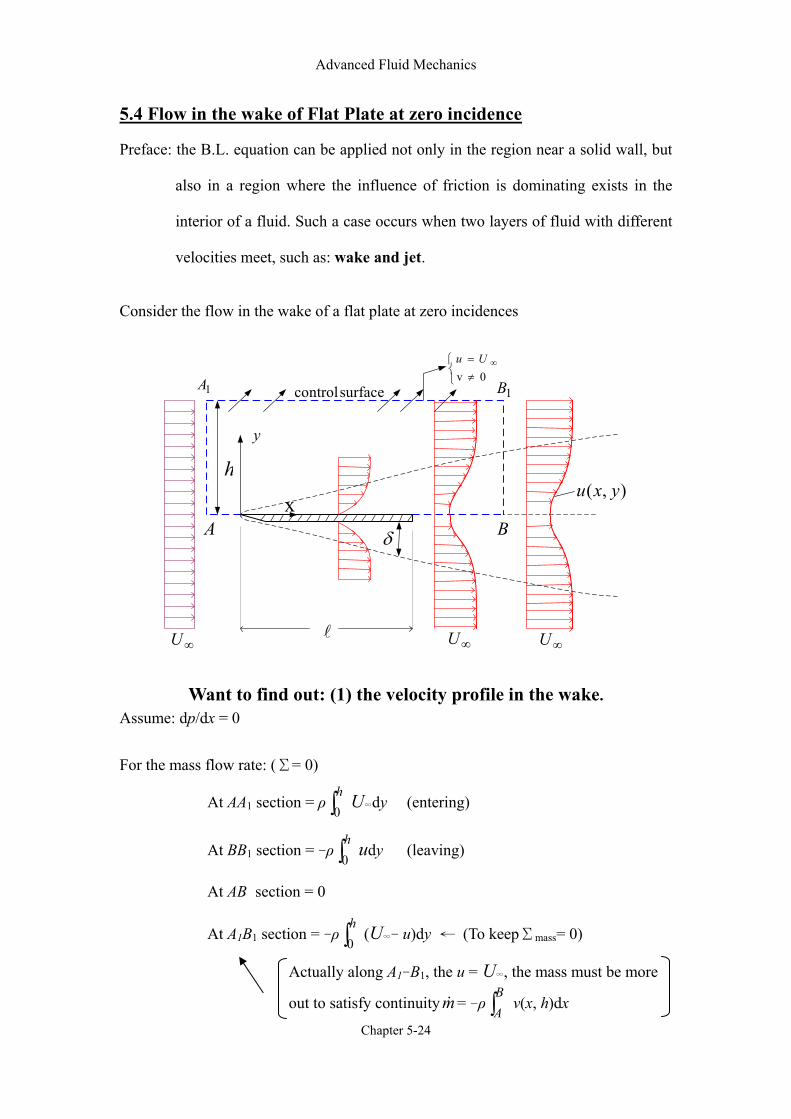
Advanced Fluid Mechanics
Chapter 5-24
5.4 Flow in the wake of Flat Plate at zero incidence
Preface: the B.L. equation can be applied not only in the region near a solid wall, but
also in a region where the influence of friction is dominating exists in the
interior of a fluid. Such a case occurs when two layers of fluid with different
velocities meet, such as: wake and jet.
Consider the flow in the wake of a flat plate at zero incidences
l
y
∞U ∞U∞U
δ
1A
A
1B
Bx
h
surface control
≠= ∞
0vUu
),( yxu
Want to find out: (1) the velocity profile in the wake. Assume: dp/dx = 0 For the mass flow rate: (Σ= 0)
At AA1 section = ρ ∫h0
U∞dy (entering)
At BB1 section = -ρ ∫h0
udy (leaving)
At AB section = 0
At A1B1 section = -ρ ∫h0
(U∞- u)dy ← (To keepΣmass= 0)
Actually along A1-B1, the u = U∞, the mass must be more
out to satisfy continuity m& = -ρ ∫BA
v(x, h)dx
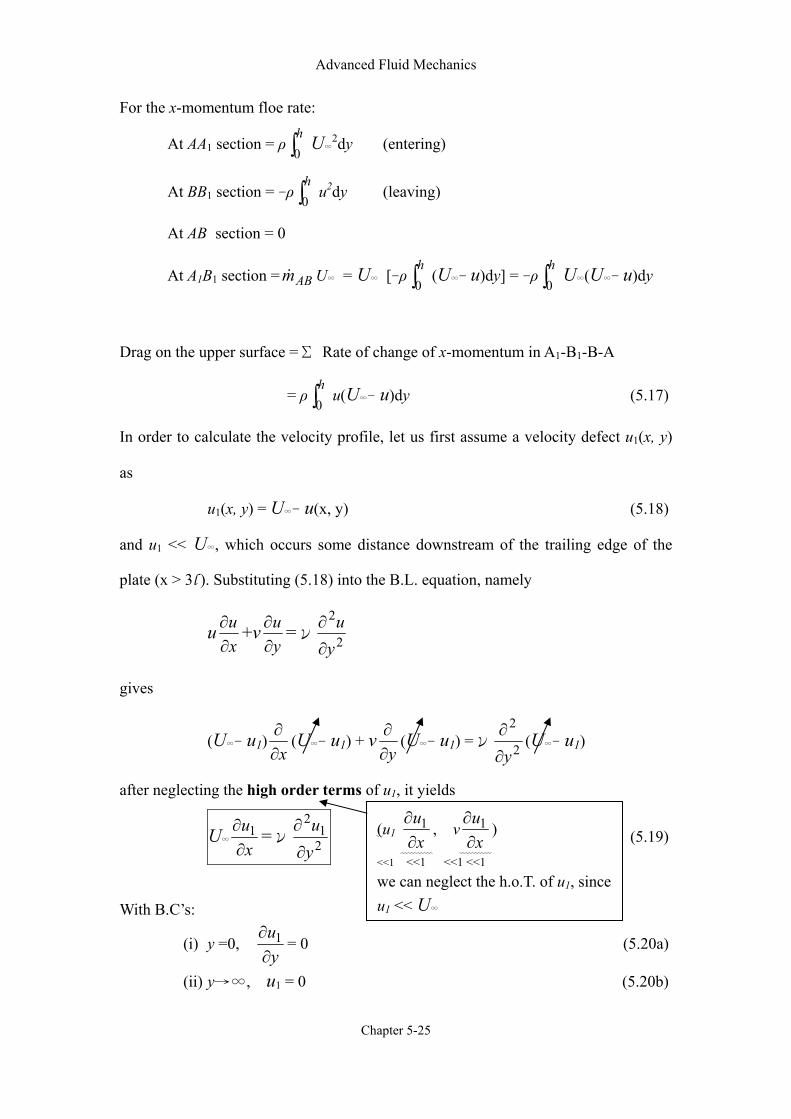
Advanced Fluid Mechanics
Chapter 5-25
For the x-momentum floe rate:
At AA1 section = ρ ∫h0
U∞2dy (entering)
At BB1 section = -ρ ∫h0
u2dy (leaving)
At AB section = 0
At A1B1 section = ABm& U∞ = U∞ [-ρ ∫h0
(U∞- u)dy] = -ρ ∫h0
U∞(U∞- u)dy
Drag on the upper surface =Σ Rate of change of x-momentum in A1-B1-B-A
= ρ ∫h0
u(U∞- u)dy (5.17)
In order to calculate the velocity profile, let us first assume a velocity defect u1(x, y)
as
u1(x, y) = U∞- u(x, y) (5.18)
and u1 << U∞, which occurs some distance downstream of the trailing edge of the
plate (x > 3l ). Substituting (5.18) into the B.L. equation, namely
uxu∂∂ +v
yu∂∂ =ν 2
2
yu
∂
∂
gives
(U∞- u1)x∂∂
(U∞- u1) + vy∂∂
(U∞- u1) =ν 2
2
y∂∂
(U∞- u1)
after neglecting the high order terms of u1, it yields
U∞
xu∂∂ 1 =ν 2
12
yu
∂
∂ (5.19)
With B.C’s:
(i) y =0, yu∂∂ 1 = 0 (5.20a)
(ii) y→∞, u1 = 0 (5.20b)
(u1 xu∂∂ 1 , v
xu∂∂ 1 )
<<1 <<1 <<1 <<1
we can neglect the h.o.T. of u1, since u1 << U∞
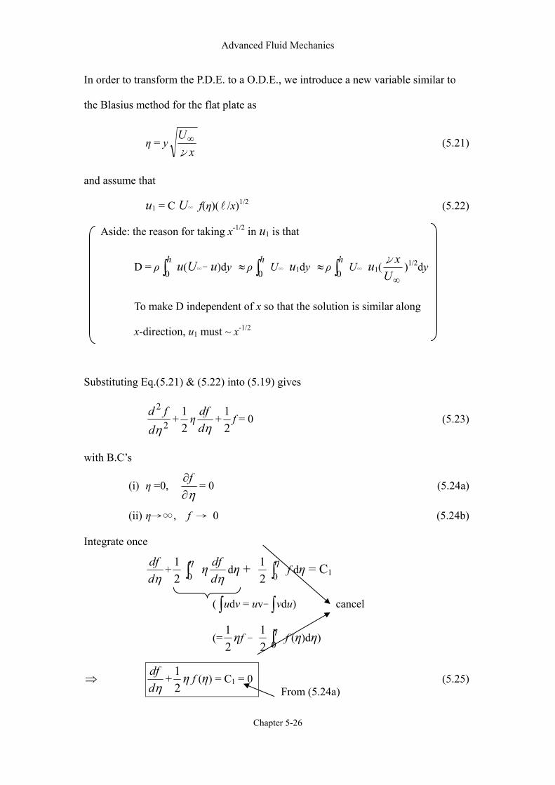
Advanced Fluid Mechanics
Chapter 5-26
In order to transform the P.D.E. to a O.D.E., we introduce a new variable similar to
the Blasius method for the flat plate as
η = yx
Uν
∞ (5.21)
and assume that
u1 = C U∞ f(η)(l /x)1/2 (5.22)
Aside: the reason for taking x-1/2 in u1 is that
D = ρ ∫h0
u(U∞- u)dy ≈ ρ ∫h0
U∞ u1dy ≈ ρ ∫h0
U∞ u1(∞Uxν
)1/2dy
To make D independent of x so that the solution is similar along
x-direction, u1 must ~ x-1/2
Substituting Eq.(5.21) & (5.22) into (5.19) gives
2
2
ηdfd
+21η
ηddf
+21
f = 0 (5.23)
with B.C’s
(i) η =0, η∂∂f
= 0 (5.24a)
(ii) η→∞, f → 0 (5.24b)
Integrate once
ηd
df+
21∫η0η
ηddf
dη + 21∫η0
f dη = C1
(∫ udv = uv-∫ vdu) cancel
(=21 ηf -
21∫η0
f (η)dη)
⇒ ηd
df+
21 η f (η) = C1 = 0 (5.25)
From (5.24a)
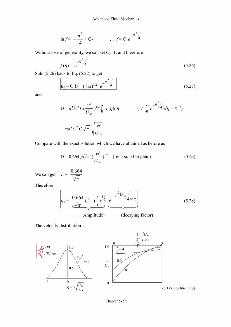
Advanced Fluid Mechanics
Chapter 5-27
ln f = 4
2η− + C2 ∴ f = C3 4
2η−e
Without lose of generality, we can set C3=1, and therefore
f (η)= 42η−
e (5.26)
Sub. (5.26) back to Eq. (5.22) to get
u1 = C U∞ (l /x)1/2 42η−
e (5.27)
and
D = ρU∞2 C(
∞Ulν
)1/2∫∞
0f (η)dη (∵ =∫
∞ −η
ηde
04
2
π1/2)
=ρU∞2 C π
∞Ulν
Compare with the exact solution which we have obtained as before as
D = 0.664 ρU∞2 (
∞Ulν
)1/2 (-one-side flat plate) (5.6a)
We can get C = π
664.0
Therefore
u1 = π
664.0 U∞ 21
)(xl x
Uye 4
2
ν∞−
(5.28)
(Amplitude) (decaying factor)
The velocity distribution is:
0.1
0 44−
5.0
max 11
uu
xUyν
∞=η
0 30.1
0
∞Uu
5.1
5.0
0
4=l
x
lν∞Uy
21
g)Schlichtinin (p.179
max1)(u1u
Advanced Fluid Mechanics
Chapter 5-28
Remark:
(1) Eq.(5.19) is a linear conduction equation, so it can actually be by separation
variables easily.
(2) A”wake” is the”defect” in stream velocity behind an immersed body in a
flow.
(3) A slender plane body with zero lift produces a smooth wake whose velocity
defects u1 decays monotonically downstream.
(4) A blunt body, such as a cylinder, has a wake distorted by an alternating shed
vortex structure.
(5) A lifting body will superimpose shed vortices of one sense.
(6) From velocity profile, we can assume boundary edge (u1/Umax ≈ 0.01)
occurs when η ~ 4 thus
η = yx
Uν
∞
→ 4 =δx
Uν
∞
∴δ =
xU
ν∞
4 = )(
4ν∞U ν
xU∞
∴δ ~ Rex1/2 (similar to the B.L. thickness growing in upper
surface of a flat plate)
(See p.22 of Van-Dyke book)
(7) In meet cases, the wake flow becomes turbulent due to the stability of the
wake flow. From velocity profile, there is a part of inflexion, which will
cause the unstability of the flow structure.

Advanced Fluid Mechanics
Chapter 5-29
5.5 Two-Dimensional Laminar Jet
Consider a 2-D Laminar Jet
The total momentum of the Jet remains constant, i.e., independent of the x, or
J =ρ ∫∞
∞−u2 dy = const (5.29)
Assume
u ~ )(' qxyf (5.30)
and the stream function
ψ ~ px f ( qxy
) = px f (η), where η = qxy
(5.31)
We now need to determine p & q.
(i) J = constant
⇒ ∫∞
∞− ∂∂ 2)(
yψ dy = independent of x.
⇒ ∫∞
∞− ∂∂
∂∂ qp x
yfx 2][ ηη
dη = ∫∞
∞−−
∂∂ qqp xfx 2][η
dη = independent of x.
⇒ power of x: ( p-q )×2 + q = 0
⇒ 2p-q = 0 (5.32)
0=dxdp
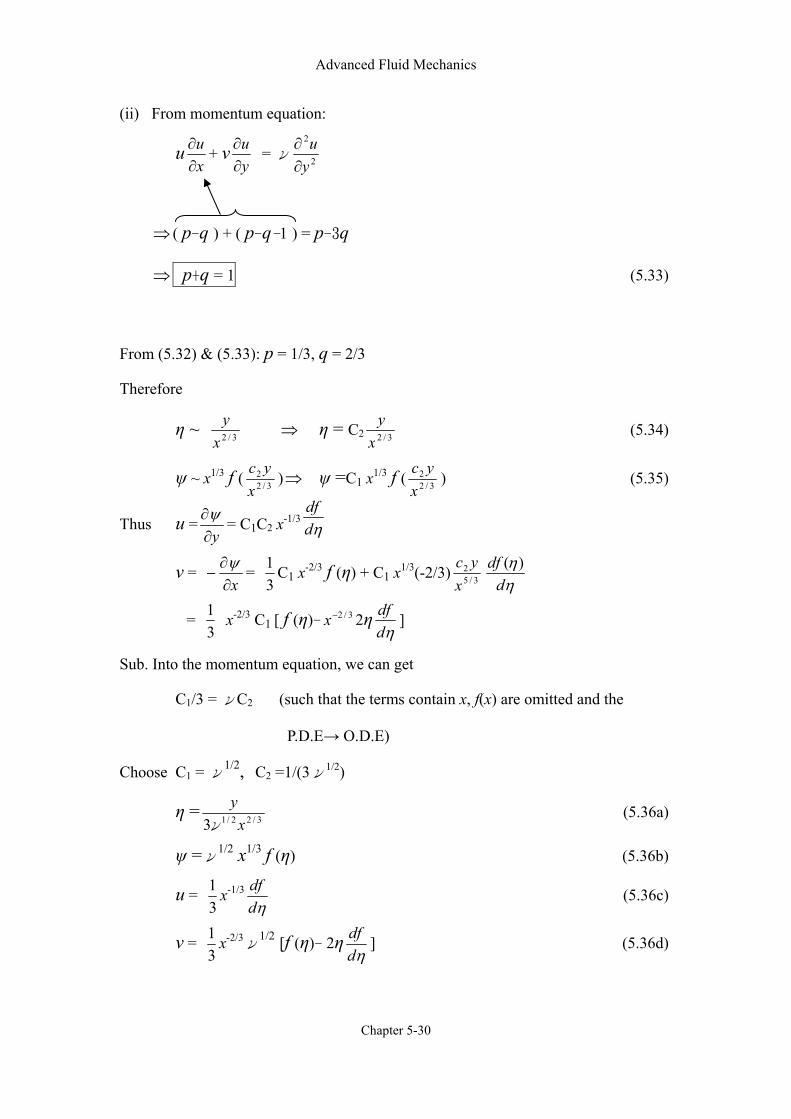
Advanced Fluid Mechanics
Chapter 5-30
(ii) From momentum equation:
uxu∂∂ + v
yu∂∂ = ν 2
2
yu
∂∂
⇒ ( p-q ) + ( p-q-1 ) = p-3q
⇒ p+q = 1 (5.33)
From (5.32) & (5.33): p = 1/3, q = 2/3
Therefore
η ~ 3/2xy ⇒ η = C2 3/2x
y (5.34)
ψ ~ x1/3 f ( 3/22
xyc )⇒ ψ =C1 x1/3 f ( 3/2
2
xyc ) (5.35)
Thus u =y∂
∂ψ = C1C2 x-1/3ηd
df
v = x∂
∂−
ψ = 31 C1 x-2/3 f (η) + C1 x1/3(-2/3) 3/5
2
xyc
ηη
ddf )(
= 31 x-2/3 C1 [ f (η)- 3/2−x 2η
ηddf ]
Sub. Into the momentum equation, we can get
C1/3 = νC2 (such that the terms contain x, f(x) are omitted and the
P.D.E→ O.D.E)
Choose C1 = ν1/2, C2 =1/(3ν1/2)
η = 3/22/13 xy
ν (5.36a)
ψ =ν1/2 x1/3 f (η) (5.36b)
u = 31 x-1/3
ηddf (5.36c)
v = 31 x-2/3ν
1/2 [f (η)- 2ηηd
df ] (5.36d)
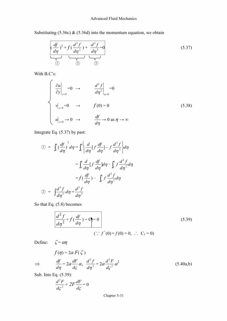
Advanced Fluid Mechanics
Chapter 5-31
Substituting (5.36c) & (5.36d) into the momentum equation, we obtain
(ηd
df )2 + f ( 2
2
ηdfd ) + 3
3
ηdfd =0 (5.37)
1 2 3
With B.C’s:
0=∂
∂
yyu =0 →
02
2
=ηηdfd =0
0=y
v =0 → f (0) = 0 (5.38)
0=y
u → 0 → ηd
df → 0 as η → ∞
Integrate Eq. (5.37) by past:
1 = ηη
ηd
ddf 2
0)(∫ = η
ηηηη
dd
fdfddff
dd
∫
−0 2
2
][
= ηηη
ηd
ddff
dd
∫0 ][ - ηη
ηd
dfdf∫0 2
2
= f (ηd
df ) - ηη
ηd
dfdf∫0 2
2
2 = ∫ ηη
dd
fd3
3
= 2
2
ηdfd
So that Eq. (5.8) becomes
2
2
ηdfd
+ f (ηd
df ) = C1= 0 (5.39)
(∵ )0(''f = f (0) = 0, ∴ C1 = 0)
Define: ζ = aη
f (η) = 2a F( ζ )
⇒ ηd
df = 2aςd
dF a, 2
2
ηdfd = 2a 2
2
ςdFd a2 (5.40a,b)
Sub. Into Eq. (5.39):
2
2
ςdFd + 2F
ςddF = 0
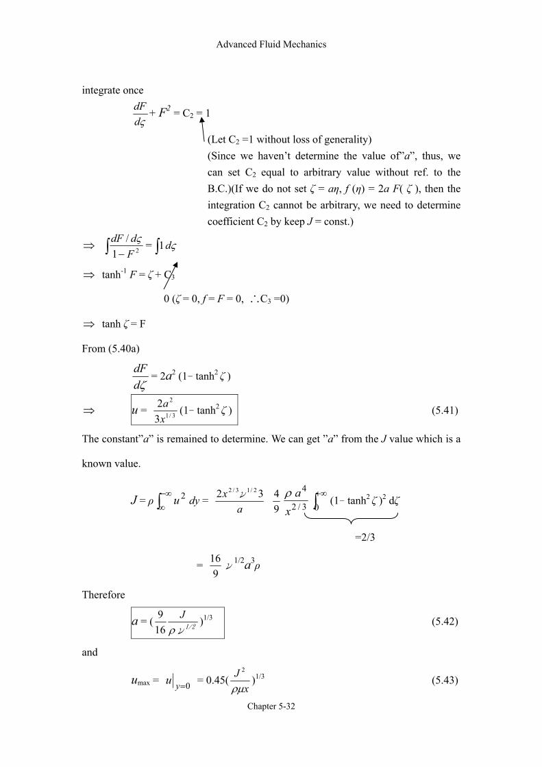
Advanced Fluid Mechanics
Chapter 5-32
integrate once
ςd
dF + F2 = C2 = 1
(Let C2 =1 without loss of generality) (Since we haven’t determine the value of”a”, thus, we can set C2 equal to arbitrary value without ref. to the B.C.)(If we do not set ζ = aη, f (η) = 2a F( ζ ), then the integration C2 cannot be arbitrary, we need to determine coefficient C2 by keep J = const.)
⇒ ∫ − 21/FddF ς = ∫ ςd 1
⇒ tanh-1 F = ζ + C3
0 (ζ = 0, f = F = 0, ∴C3 =0)
⇒ tanh ζ = F
From (5.40a)
ζd
dF= 2a2 (1- tanh2 ζ )
⇒ u = 3/1
2
32xa (1- tanh2 ζ ) (5.41)
The constant”a” is remained to determine. We can get ”a” from the J value which is a
known value.
J = ρ ∫−∞
∞2u dy =
ax 32 2/13/2 ν
94
3/2
4 x
aρ∫+∞
0(1- tanh2 ζ )2 dζ
=2/3
= 9
16ν
1/2a3ρ
Therefore
a = (1/2νρ
J169 )1/3 (5.42)
and
umax = 0=yu = 0.45(x
Jρµ
2
)1/3 (5.43)

Advanced Fluid Mechanics
Chapter 5-33
The volume rate of discharge across any vertical plane is
Q& = ∫∞
∞−udy = 3.3019(
ρxJν )1/3 (5.44)
or m& = ρQ& = 3.3019( Jρµx )1/3
From Eq.(5.43) we know that the max axial velocity decreases as x increases.
However, from Eq.(5.44) we downstream direction, because fluid particles are carried
away with the jet owing to friction on its boundary. It also increases with increasing
momentum.
Remark:
(1) Note that m& ~ x1/3 because the jet entrains ambient fluid by dragging it
along. However, Eq.(5.44) implies falsely that m& =0, which is the slot
where the Re ~ µm& ~ ( 2
µρ xJ
)1/3. The B.L. theory is not valid for Re is small.
Therefore, we cannot ascertain any details of the flow near the jet outlet
with B.L. theory.
(2) Since jet velocity profile are S-Shaped (i.e. have a point of inflection), they
are unstable and undergo transition to turbulent early – at a Re of about 30,
based on exist slot width and mean slot velocity.
(3) Define the width of the jet as twice the distance y where u = 0.01 umax, we
then have
Width = 2maxu %1=u
y ≈ 2.18(ρµ
Jx 22
)1/3
Thus Width ~ x2/3 and ~ J -1/3
Advanced Fluid Mechanics
Chapter 6-1
Chapter 6 Approximate methods for the Solution of the 2-D,
steady B.L. Equations
In the history of the developing the B.L. flow, we have:
(1) Analysis solution (exact solution): A exact solution consists every term in the
B.L. equation although some of terms may be identically zero. We do not imply
that an exact solution is one in a closed form; it could be a convergent series.
→ For as complex geometry (specially with pressure gradient), this method is
difficult and sometimes impossible. We have discussed some simple case in the
previous chapter.
(2) Approximate Solutions: All approximate methods are integral methods which
do not attempt to satisfy the B.L. equation for every streamline; instead, the
equations are satisfied only on an average extended over the thickness of the
B.L. → well-suited to the generation of a quick outline of a solution even in
more complex cases. This technique is important before the advent of fast
computer.
Advanced Fluid Mechanics
Chapter 6-2
6.1 Karman’s Integral Momentum Relation
Consider a steady, 2-D, compressible flow:
Continuity:
t∂
∂ρ+∇.(ρV
v) = 0
xu∂
)(ρ+
yv
∂∂ )(ρ
= 0 (6.1)
B.L. Eq:
ρ[uxu∂∂
+vyu∂∂
] = dxdp
− +y∂∂
[μyu∂∂
]
Since ρuxu∂∂
+ρvyu∂∂
= [ρuxu∂∂
+ρvyu∂∂
] + [xu∂
)(ρ+
yv
∂∂ )(ρ
].u
= [ρuxu∂∂
+ uxu∂
)(ρ] + [ρv
yu∂∂
+ uyv
∂∂ )(ρ
]
= x∂∂
(ρu2) + y∂∂
(ρuv)
∴ x∂∂
(ρu2) + y∂∂
(ρuv) = dxdp
− +y∂∂
[μyu∂∂
] (6.2)
Integrate the continuity equation from y = 0 to y =δ:
∫δ0 x
u∂
)(ρdy +∫
δ0 y
v∂
∂ )(ρdy = 0
(Leibnitz’s rule)
x∂∂∫δ0ρu dy -ρe ue dx
dδ +ρe ue -ρ0 u0 = 0
⇒ ve = eρ
1∂∂
− ∫δ0x
ρu dy +ρe ue dxdδ
+ρ0 u0 (6.3)
Integrate the B.L. equation:
∫δ0 x
u∂
)( 2ρdy +∫
δ0 y
uv∂
∂ )(ρdy = ∫ −
δ0
)(dxdp
dy +∫δ0 y∂
∂(μ
yu∂∂
) dy
1 2 3 4

Advanced Fluid Mechanics
Chapter 6-3
1 = x∂∂∫δ0ρu2 dy-ρe ue
2
dxdδ ( Leibnitz’s Rule)
2 = ρe ue ve-ρ0 u0 v0 =ρe ue ve = ue [ ∫∂∂
−δ0x
ρu dy +ρe ue dxdδ
+ρ0 u0]
(=0, ∵ u0 = 0) (Eq.(6.3))
3 = )(dxdp
− δ (∵dxdp
= fn(x) only from the B.L. Theory)
4 =μ(yu∂∂
)y=δ-μ(yu∂∂
)y=0 = -τ0
Therefore, the B.L. equation becomes
x∂∂∫δ0ρu2 dy-ρe ue
2
dxdδ
-ue ∫∂∂ δ
0xρu dy +ρe ue
2 dx
dδ+ρ0 u0
= )(dxdp
− δ -τ0 (6.4)
If we evaluate the B.L. equation at y =δ, we have
ρ[ue xu∂∂
+ ve yu∂∂
] = dxdp
− + y∂∂
[μyu∂∂
]
=0 ( = 0 at y =δ)
ρue dxdue =
dxdp
− (6.5a)
Also
ue ∫∂∂ δ
0xρu dy =
x∂∂
[ ue∫δ0 ρu dy ]-
dxdue ∫
δ0 ρu dy
= x∂∂
[ ∫δ0 ρu ue dy ]-
dxdue ∫
δ0 ρu dy (6.5b)
Sub. (6.5a) & (6.5b) into (6.4), we have
x∂∂∫δ0
(ρu2-ρu ue)dy +
dxdue ∫
δ0 ρu dy -ρe ue dx
due δ+ ueρ0 v0 = -τ0
or
dxd
ρe ue2 ∫
δ0 eeu
uρρ
(1eu
u− )dy +ρe ue dx
due ∫δ0 [1
eeuu
ρρ
− ]dy-ueρ0 v0 = -τ0
at y =δ
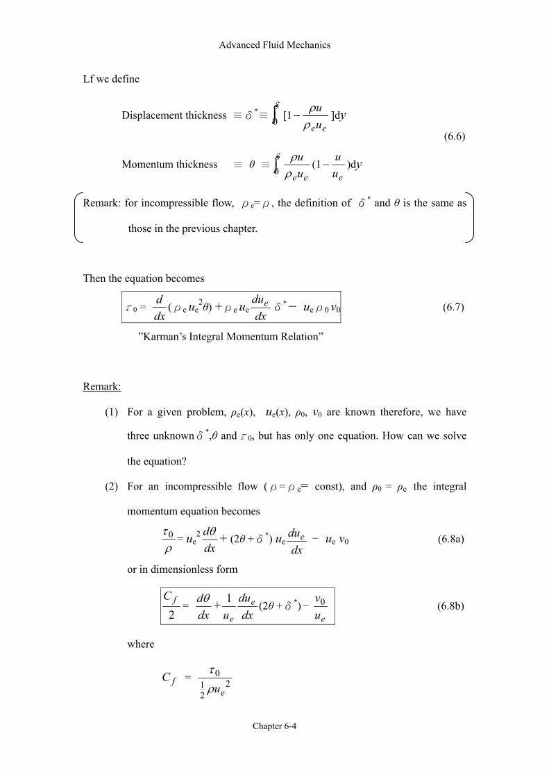
Advanced Fluid Mechanics
Chapter 6-4
Lf we define
Displacement thickness ≡δ*≡∫δ0 [1
eeuu
ρρ
− ]dy
Momentum thickness ≡ θ ≡∫δ0 eeu
uρρ
(1eu
u− )dy
Remark: for incompressible flow, ρe=ρ, the definition of δ* and θ is the same as
those in the previous chapter.
Then the equation becomes
τ0 = dxd
(ρe ue2θ) +ρe ue dx
due δ*- ueρ0 v0 (6.7)
”Karman’s Integral Momentum Relation”
Remark:
(1) For a given problem, ρe(x), ue(x), ρ0, v0 are known therefore, we have
three unknownδ*,θ andτ0, but has only one equation. How can we solve
the equation?
(2) For an incompressible flow (ρ=ρe= const), and ρ0 = ρe the integral
momentum equation becomes
ρτ 0 = ue
2
dxdθ + (2θ +δ*) ue
dxdue - ue v0 (6.8a)
or in dimensionless form
2
fC=
dxdθ +
dxdu
ue
e
1(2θ +δ*) -
euv0 (6.8b)
where
fC = 221
0
euρτ
(6.6)
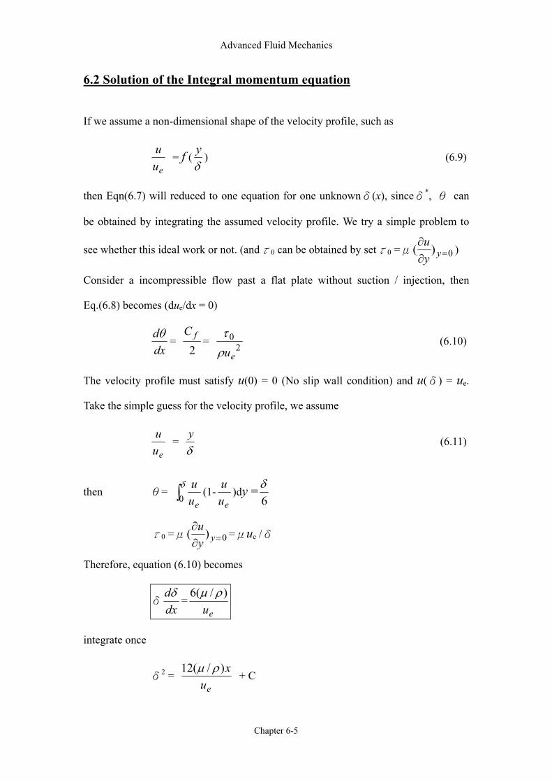
Advanced Fluid Mechanics
Chapter 6-5
6.2 Solution of the Integral momentum equation If we assume a non-dimensional shape of the velocity profile, such as
eu
u = f (
δy
) (6.9)
then Eqn(6.7) will reduced to one equation for one unknownδ(x), sinceδ*, θ can
be obtained by integrating the assumed velocity profile. We try a simple problem to
see whether this ideal work or not. (andτ0 can be obtained by setτ0 =μ 0)( =∂∂
yyu
)
Consider a incompressible flow past a flat plate without suction / injection, then
Eq.(6.8) becomes (due/dx = 0)
dxdθ
= 2
fC= 2
0
euρτ
(6.10)
The velocity profile must satisfy u(0) = 0 (No slip wall condition) and u(δ) = ue.
Take the simple guess for the velocity profile, we assume
eu
u =
δy
(6.11)
then θ= ∫δ0 eu
u(1-
euu
)dy =6δ
τ0 =μ 0)( =∂∂
yyu
=μue /δ
Therefore, equation (6.10) becomes
δdxdδ
=eu
)/(6 ρµ
integrate once
δ2 = eu
x)/(12 ρµ + C
Advanced Fluid Mechanics
Chapter 6-6
Sinceδ(x = 0) = 0 ⇒ C = 0
The boundary layer thickness is thus
δ(x) = eu
x)/(12 ρµ
or xδ
= xueρµ12
= 3.46 Rex-1/2 (6.12a)
The friction coefficient Cf is
Cf = 221
e
w
uρτ
= 221
/
e
e
uuρ
δµ = 0.577 Rex
-1/2 (6.12b)
From the exact solution as shown in chapter 5, we have obtained
xδ
= 5 Rex-1/2 (5.4)
and Cf = 0.664 Rex-1/2 (5.5a)
Thus, this simple analysis has achieved the correct dependence on Rex, bit fairly good
numerical values for the coefficients.
Question: Any better velocity profiles or better methods?
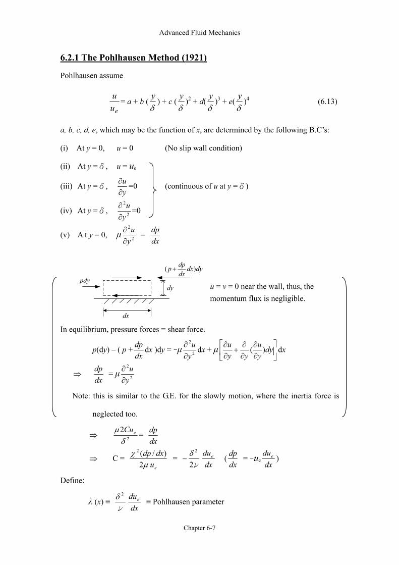
Advanced Fluid Mechanics
Chapter 6-7
dy
dx
pdy
dydxdxdpp )( +
6.2.1 The Pohlhausen Method (1921)
Pohlhausen assume
eu
u= a + b (
δy
) + c (δy
)2 + d(δy
)3 + e(δy
)4 (6.13)
a, b, c, d, e, which may be the function of x, are determined by the following B.C’s:
(i) At y = 0, u = 0 (No slip wall condition)
(ii) At y =δ, u = ue
(iii) At y =δ, yu∂∂ =0 (continuous of u at y =δ)
(iv) At y =δ, 2
2
yu
∂∂ =0
(v) A t y = 0, µ 2
2
yu
∂∂ =
dxdp
In equilibrium, pressure forces = shear force.
p(dy) – ( p +dxdp dx )dy = -µ 2
2
yu
∂∂ dx + µ
∂∂
∂∂
+∂∂ dy
yu
yyu )( dx
⇒ dxdp = µ 2
2
yu
∂∂
Note: this is similar to the G.E. for the slowly motion, where the inertia force is
neglected too.
⇒ 2
2δ
µ eCu=
dxdp
⇒ C = eudxdp
2)/(2
µχ =
ν2
2δ−
dxdue (
dxdp = -ue dx
due )
Define:
λ (x) ≡ ν
2δdxdue ≡ Pohlhausen parameter
u = v = 0 near the wall, thus, the momentum flux is negligible.
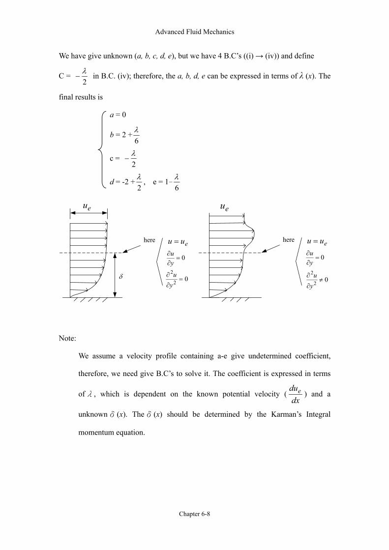
Advanced Fluid Mechanics
Chapter 6-8
We have give unknown (a, b, c, d, e), but we have 4 B.C’s ((i) → (iv)) and define
C = 2λ
− in B.C. (iv); therefore, the a, b, d, e can be expressed in terms of λ (x). The
final results is
a = 0
b = 2 +6λ
c = 2λ
−
d = -2 +2λ , e = 1-
6λ
here
δ
eu
euu =
0=∂∂
yu
02
2=
∂
∂
yu
eu
here euu =
0=∂∂
yu
02
2≠
∂
∂
yu
Note:
We assume a velocity profile containing a-e give undetermined coefficient,
therefore, we need give B.C’s to solve it. The coefficient is expressed in terms
ofλ, which is dependent on the known potential velocity (dx
due ) and a
unknownδ(x). Theδ(x) should be determined by the Karman’s Integral
momentum equation.
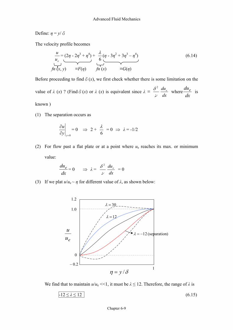
Advanced Fluid Mechanics
Chapter 6-9
Define: η = y/δ
The velocity profile becomes
eu
u = (2η - 2η3 + η4) + 6λ (η - 3η2 + 3η3 – η4) (6.14)
fn (x, y) ≡F(η) fn (x) ≡G(η)
Before proceeding to findδ(x), we first check whether there is some limitation on the
value of λ (x) ? (Findδ(x) or λ (x) is equivalent since λ ≡ ν
2δdxdue where
dxdue is
known )
(1) The separation occurs as
0=∂
∂
yyu = 0 ⇒ 2 +
6λ = 0 ⇒ λ = -1/2
(2) For flow past a flat plate or at a point where ue reaches its max. or minimum
value:
dx
due = 0 ⇒ λ = ν
2δdxdue = 0
(3) If we plat u/ue ~ η for different value of λ, as shown below:
2.1
0.1
0
2.0−1
δη /y=
euu
)separation( 12−=λ
12=λ
30=λ
We find that to maintain u/ue <<1, it must be λ ≤ 12. Therefore, the range of λ is
-12 ≤ λ ≤ 12 (6.15)

Advanced Fluid Mechanics
Chapter 6-10
By the velocity profile given in Eqn (6.14), we get
δ* = δ(12010
3 λ− )
θ = 63δ (
14415537 2λλ
−− ) (6.16)
τ0 =μ0
)(=∂
∂
yyu =
δµ eu
(2 +6λ )
Next step is to solve the integral momentum equation in terms of λ (x). For
incompressible flow without wall injection/ suction, Eq. (6.8a) gives
euµθτ 0 =
νeu θ
dxdθ + ( 2 +
θδ *
)ν
2θdxdue (6.17)
Note that equation (6.17) do not containδ(x) explicitly. We thus try to solve θ(x), and
then deduceδfrom it with the cuds of Eq.(6.16).
Introduce
Z ≡ ν
2θ λ
K ≡ ν
2θdxdue ⇒ K = Z
dxdue = (
δθ )2
ν
2δdxdue
= (31537
-945λ
-9072
2λ )2 λ (6.18a)
Denote
θδ *
=2
90721
9451
31537
1201
103
λλ
λ
−−
− ≡ f1 (K) (shape-factor correlation) (6.18b)
and
euµθτ 0 = (2 +
6λ )(
31537
-945λ
-9072
2λ ) ≡ f2 (K) (6.18c)
Also note that
ν
θdxdθ =
dxd
21 (
ν
2θ ) = dxdZ
21
(6.16)→
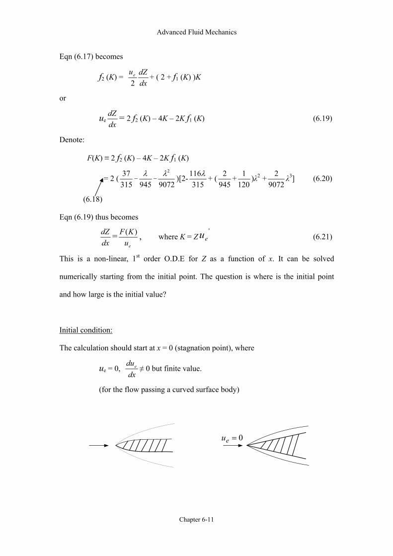
Advanced Fluid Mechanics
Chapter 6-11
Eqn (6.17) becomes
f2 (K) = dxdZue
2+ ( 2 + f1 (K) )K
or
ue dxdZ = 2 f2 (K) – 4K – 2K f1 (K) (6.19)
Denote:
F(K) ≡ 2 f2 (K) – 4K – 2K f1 (K)
= 2 (31537
-945λ
-9072
2λ )[2-315
116λ + (945
2 +120
1 )λ2 +9072
2 λ3] (6.20)
(6.18)
Eqn (6.19) thus becomes
dxdZ =
euKF )( , where K = Z
'eu (6.21)
This is a non-linear, 1st order O.D.E for Z as a function of x. It can be solved
numerically starting from the initial point. The question is where is the initial point
and how large is the initial value?
Initial condition:
The calculation should start at x = 0 (stagnation point), where
ue = 0, dxdue ≠ 0 but finite value.
(for the flow passing a curved surface body)
0=eu
Advanced Fluid Mechanics
Chapter 6-12
Since dxdZ =
euKF )(
That is, F(K) must be zero at the stagnation point, otherwise, dxdZ will become infinite,
which is physically meaningless. Therefore, at x = 0
F(K) = 0 λ = λ0 = 7.052
or K = K0 = 0.0770
The initial value of Z and dZ/dx are
Z0 =
0
0
=x
e
dxdu
K =
0
077.0
=x
e
dxdu
(dxdZ )0 = (
euKF )( )0 = (
dxdudxdK
dKdF
e /)0 = -0.0652
20
02
2
)(
)(
=
=
xe
xe
dxdudx
ud
Hosptial Rule (6.20)(6.18a)
Computational procedure:
(1) ue (x), dxdue , and
02
2
=x
e
dxud
are given by potential flow.
(2) Integral Eq.(6.21) → Z(x) & K(x)
(3) By equation of K =ν
2θdxdue → θ(x)
(4) By equation (6.18a) → λ (x)
(5) By (6.18b) & (6.18c) →δ*,τ0
(6) By (6.16) →δ
(7) By (6.14) → u / ue
The calculation is continuous until λ (x) = -12 or K = -0.1567, where the separation
occurs.
Eq. (6.20)

Advanced Fluid Mechanics
Chapter 6-13
Example: For a flat plate case.
dxdue = 0 → λ (x) =
ν
2δdxdue = 0
The assumed velocity profile (6.14) becomes
eu
u = 2η - 2η3 + η4
(6.18) ⇒ K = Zdx
due =0
(6.20) ⇒ F(0) = F(K) = 2(31537
)(2) = 0.1698
(6.21) ⇒ dxdZ =
euKF )( =
eu4698.0
∴ Z = eu
4698.0x + C
Since x = 0, Z = 0 (why?) →
∴ Z = eu
4698.0x = …..
From (6.16) with λ = 0, it yields
δδ *
= 0.3, δθ
= 631
(5
37) = 0.1174, τ0 =
δµ eu 2
(6.22)
From exact solution, we know
δ= 5eu
νx, δ* =1.7208
eu
νx, θ=0.664
eu
νx
τ0 = 0.332μue (νx
eu)1/2
Take eu
u= a + b (
δy
) + c (δy
)2 +…..
since shape edge flat plate (dxdue = 0), and Z
=ν
2δ), at x = 0, δ= 0 ∴ Z = 0 at x = 0.
don’t need this procedure
to get δδ *
,δθ
, andτ0
Advanced Fluid Mechanics
Chapter 6-14
With λ = 0, (dxdue = 0), we have
δδ *
= 0.3, δθ
= 0.1174, τ0 = δµ eu 2
Sub. into the Karman Integral equation
euµθτ 0 =
νeuθ
dxdθ
(δµ eu 2
)(0.11748)(euµ
1) = (0.11748δ)(
νeu
)dxd
[0.11748]
⇒ 0.2348 = (0.0138)ν
euδ
dxdδ
⇒ 17.015eu
ν=δ
dxdδ
=21
dxd )( 2δ
⇒ dx
d )( 2δ= 34.03
eu
ν
⇒ δ2 =34.03eu
νx
⇒ δ = 5.83eu
νx or
xδ
= 5.83 Rex-1/2
And the exact solution isδ= 5eu
νx, therefore, the Pohlhausen Method is closed
exact solution than taking eu
u=
δy
case.
Therefore, δδ *
= 5
7208.1= 0.344
δθ
= 5664.0
= 0.1328 (6.23)
τ0 = 0.332μue (δ5
) = 1.66δµ eu
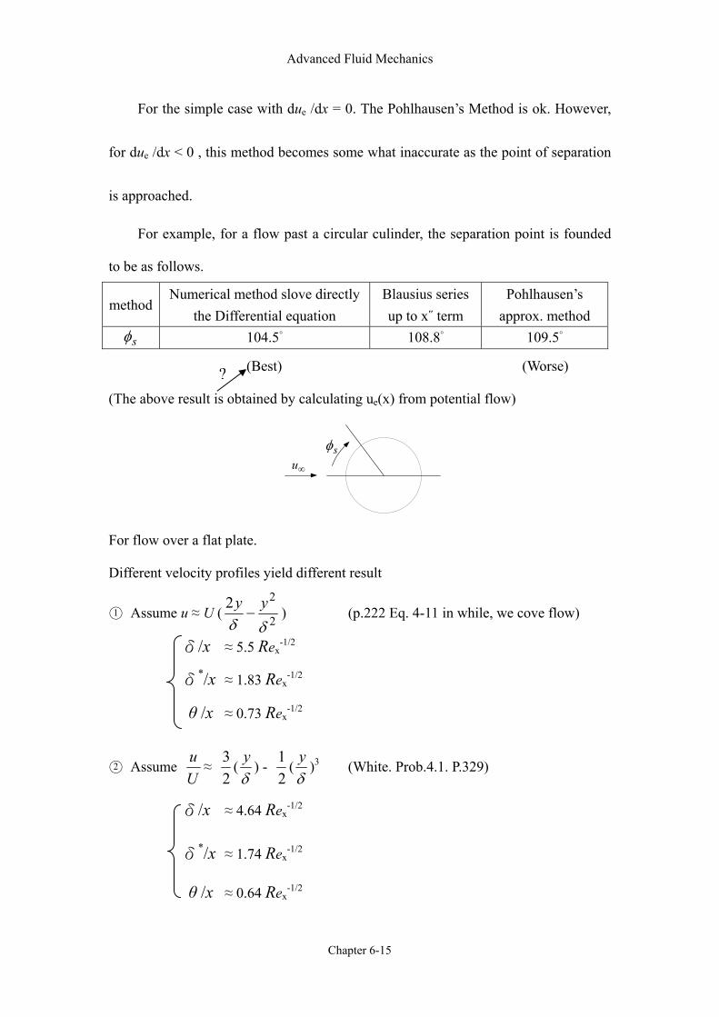
Advanced Fluid Mechanics
Chapter 6-15
For the simple case with due /dx = 0. The Pohlhausen’s Method is ok. However,
for due /dx < 0 , this method becomes some what inaccurate as the point of separation
is approached.
For example, for a flow past a circular culinder, the separation point is founded
to be as follows.
method Numerical method slove directly
the Differential equation Blausius series up to x˝ term
Pohlhausen’s approx. method
sφ 104.5° 108.8° 109.5°
(Best) (Worse)
(The above result is obtained by calculating ue(x) from potential flow)
∞usφ
For flow over a flat plate.
Different velocity profiles yield different result
1 Assume u ≈ U ( 2
22δδyy
− ) (p.222 Eq. 4-11 in while, we cove flow)
δ/x ≈ 5.5 Rex-1/2
δ*/x ≈ 1.83 Rex-1/2
θ /x ≈ 0.73 Rex-1/2
2 Assume Uu≈
23
(δy
) - 21
(δy
)3 (White. Prob.4.1. P.329)
δ/x ≈ 4.64 Rex-1/2
δ*/x ≈ 1.74 Rex-1/2
θ /x ≈ 0.64 Rex-1/2
?
Advanced Fluid Mechanics
Chapter 6-16
3 Assume Uu≈ sin (
δπ2
y) (White. Prob.4.3 p.330)
δ/x ≈ 4.80 Rex-1/2
θ /x ≈ 0.656 Rex-1/2
(The B.C’s needed for velocity profile is described very completely on p.534 in 吳望
一編著,流體力學.(歐亞))
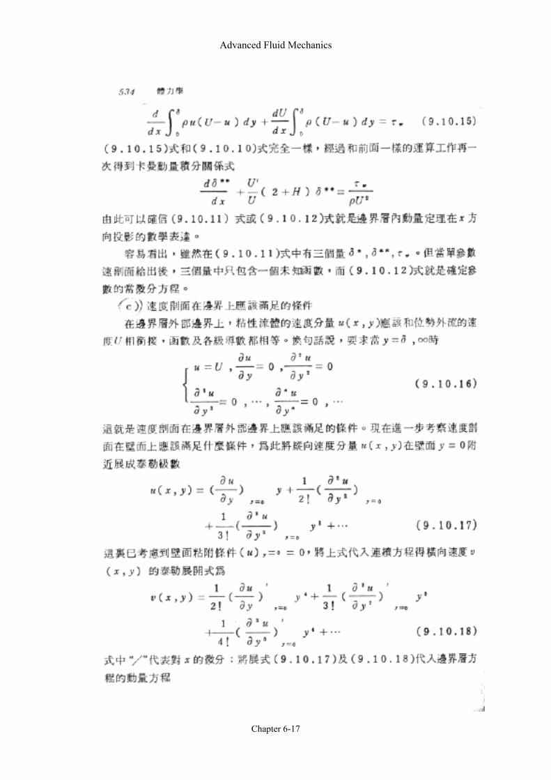
Advanced Fluid Mechanics
Chapter 6-17
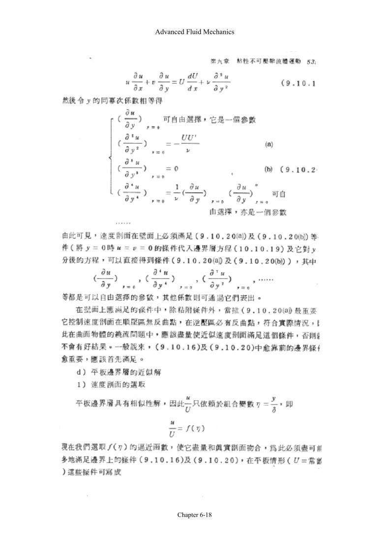
Advanced Fluid Mechanics
Chapter 6-18
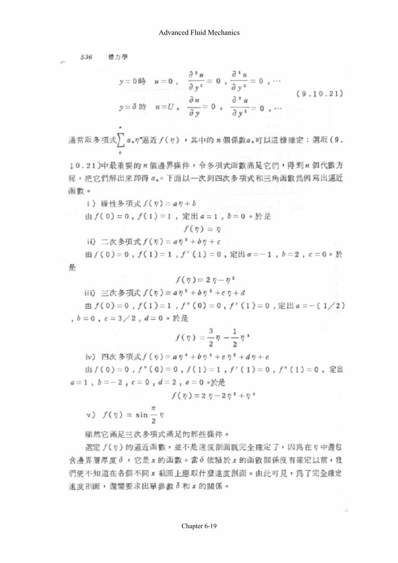
Advanced Fluid Mechanics
Chapter 6-19

Advanced Fluid Mechanics
Chapter 6-20
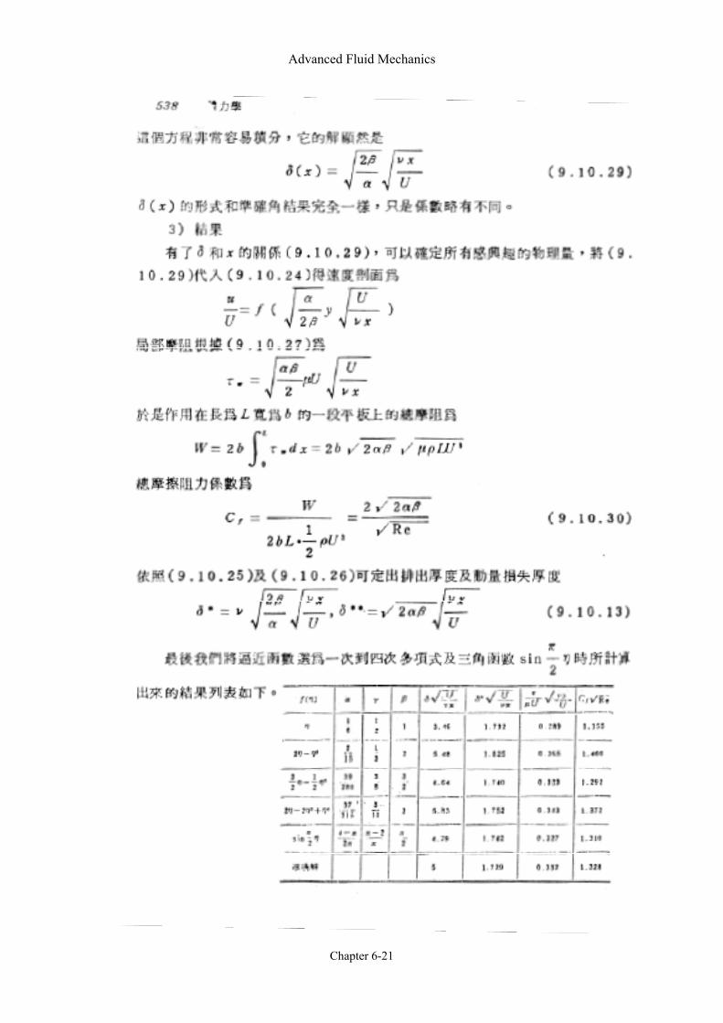
Advanced Fluid Mechanics
Chapter 6-21
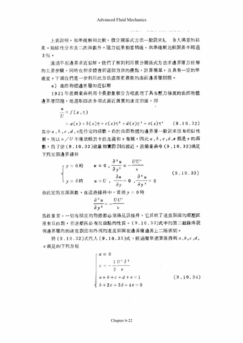
Advanced Fluid Mechanics
Chapter 6-22
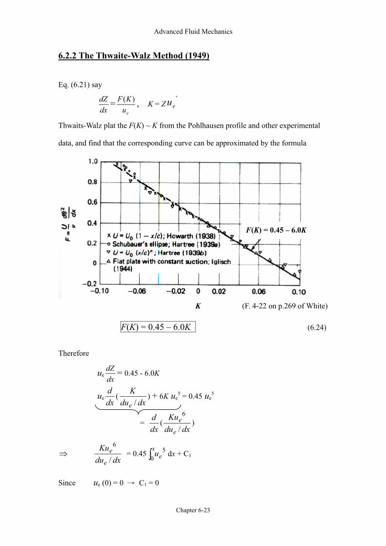
Advanced Fluid Mechanics
Chapter 6-23
6.2.2 The Thwaite-Walz Method (1949)
Eq. (6.21) say
dxdZ =
euKF )( , K = Z
'eu
Thwaits-Walz plat the F(K) ~ K from the Pohlhausen profile and other experimental
data, and find that the corresponding curve can be approximated by the formula
F(K) = 0.45 – 6.0K (6.24) Therefore
ue dxdZ = 0.45 - 6.0K
uedxd
(dxdu
K
e /) + 6K ue
5 = 0.45 ue5
= dxd
(dxdu
Ku
e
e/
6)
⇒ dxdu
Ku
e
e/
6 = 0.45 ∫
xeu
05 dx + C1
Since ue (0) = 0 → C1 = 0
F(K) = 0.45 – 6.0K
K (F. 4-22 on p.269 of White)
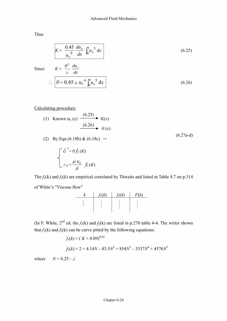
Advanced Fluid Mechanics
Chapter 6-24
Thus
K = 645.0
eu dxdue ∫
xeu
05 dx (6.25)
Since K = ν
2θdxdue
∴ θ= 0.45νue-6 ∫
xeu
05 dx (6.26)
Calculating procedure:
(1) Known ue (x) K(x)
θ(x)
(2) By Eqn (6.18b) & (6.18c) →
δ*=θf1 (K)
τ0 =δµ eu f2 (K)
The f1(k) and f2(k) are empirical correlated by Thwaits and listed in Table 4.7 on p.314
of White’s:”Viscous flow”
k f1(k) f2(k) F(k)
......
……
……
……
(In F. White, 2nd ed. the f1(k) and f2(k) are listed in p.270 table 4-4. The writer shown that f1(k) and f2(k) can be curve pitted by the following equations:
f1(k) ≈ ( K + 0.09)0.62
f2(k) ≈ 2 + 4.14N – 83.5N2 + 854N3 – 3337N4 + 4576N5
where N = 0.25 -λ
(6.25)
(6.26)
(6.27a-d)
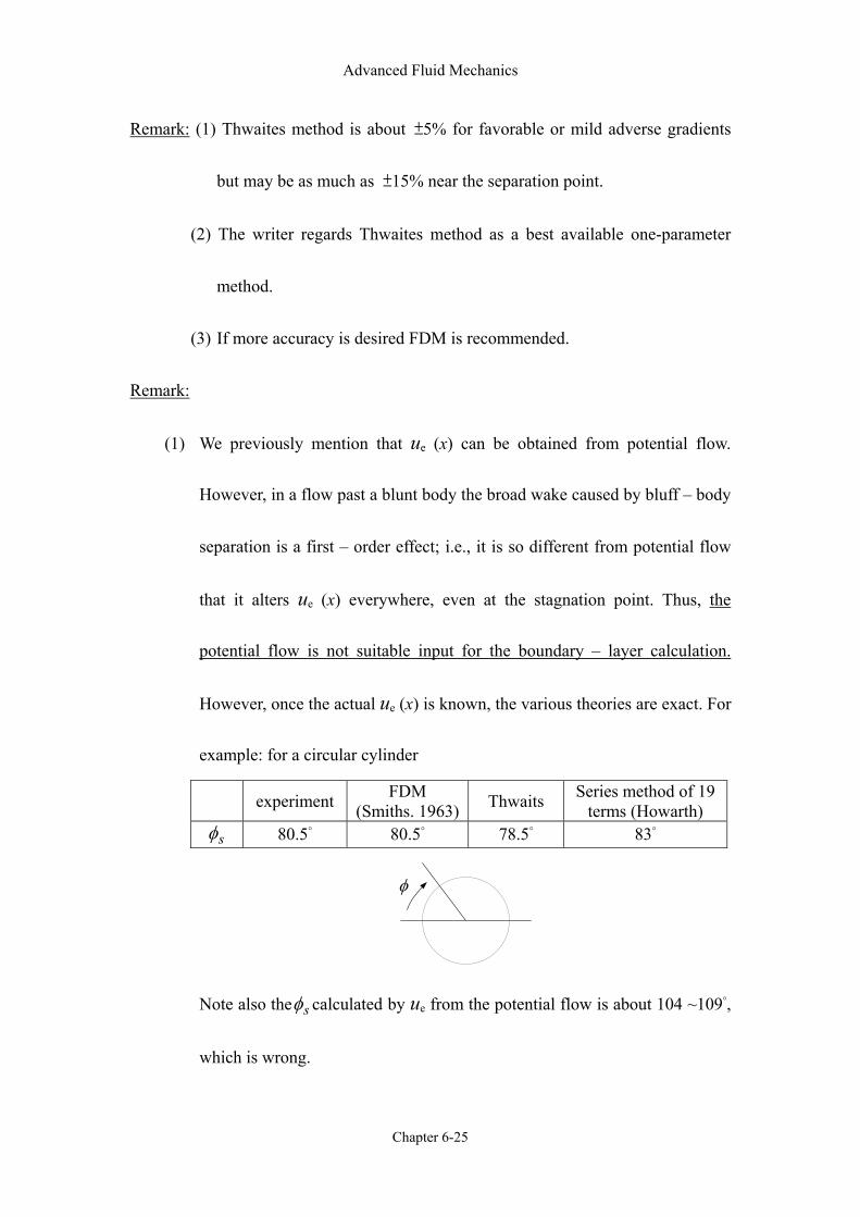
Advanced Fluid Mechanics
Chapter 6-25
Remark: (1) Thwaites method is about ±5% for favorable or mild adverse gradients
but may be as much as ±15% near the separation point.
(2) The writer regards Thwaites method as a best available one-parameter
method.
(3) If more accuracy is desired FDM is recommended.
Remark:
(1) We previously mention that ue (x) can be obtained from potential flow.
However, in a flow past a blunt body the broad wake caused by bluff – body
separation is a first – order effect; i.e., it is so different from potential flow
that it alters ue (x) everywhere, even at the stagnation point. Thus, the
potential flow is not suitable input for the boundary – layer calculation.
However, once the actual ue (x) is known, the various theories are exact. For
example: for a circular cylinder
experiment FDM (Smiths. 1963) Thwaits Series method of 19
terms (Howarth) sφ 80.5° 80.5° 78.5° 83°
φ
Note also the sφ calculated by ue from the potential flow is about 104 ~109°,
which is wrong.
Advanced Fluid Mechanics
Chapter 6-26
(2) All laminar – boundary – layer calculations hinge upon knowing the correct
ue (x). It is presently a very active area of research to develop coupled
methods in which a separating boundary layer interacts with and strongly
modifies the external inviscid flow. (e.g.: B.L/shock interaction)
(3) A higher order perturbation method or asymptotic expansion method is
applied to match the inviscid & viscous region.
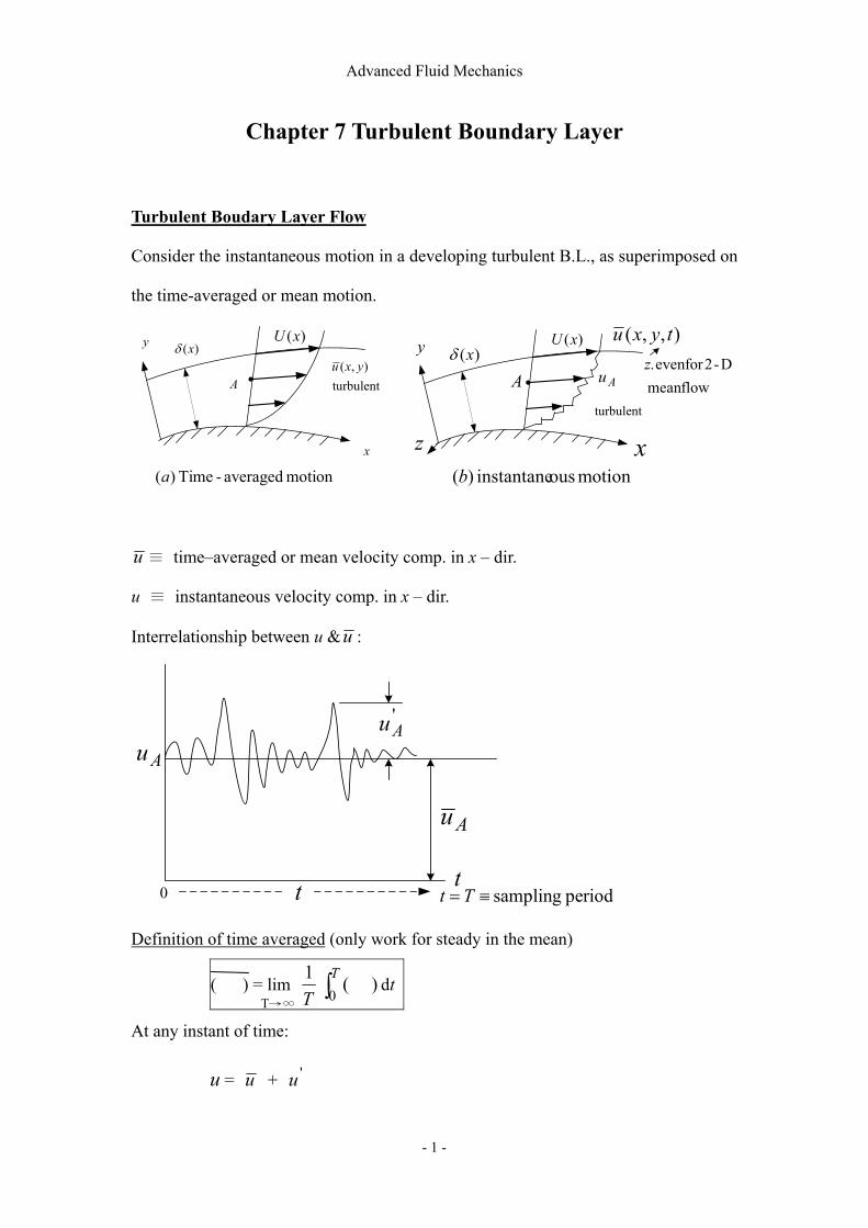
Advanced Fluid Mechanics
- 1 -
Chapter 7 Turbulent Boundary Layer
Turbulent Boudary Layer Flow
Consider the instantaneous motion in a developing turbulent B.L., as superimposed on
the time-averaged or mean motion.
x
y )(xδ
A
)(xU
turbulent),( yxu
•
motion averaged-Time )(ax
y )(xδ
A
)(xU ),,( tyxu
•
z
Au
turbulent
flowmean D-2for even .z
motion ousinstantane )(b
u ≡ time–averaged or mean velocity comp. in x – dir.
u ≡ instantaneous velocity comp. in x – dir.
Interrelationship between u &u :
'Au
Au
t
Au
0 t period sampling ≡=Tt
Definition of time averaged (only work for steady in the mean)
( ) = lim T1∫
T0
) ( dt
At any instant of time:
u = u + 'u
T→∞
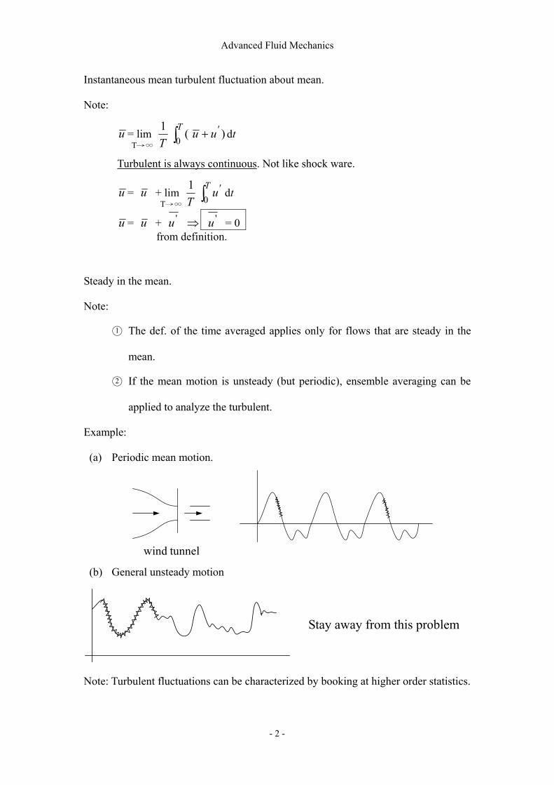
Advanced Fluid Mechanics
- 2 -
Instantaneous mean turbulent fluctuation about mean.
Note:
u = lim T1 )(
0∫ +T 'uu dt
Turbulent is always continuous. Not like shock ware.
u = u + lim T1∫
T 'u0
dt
u = u + 'u ⇒ 'u = 0 from definition.
Steady in the mean.
Note:
1 The def. of the time averaged applies only for flows that are steady in the
mean.
2 If the mean motion is unsteady (but periodic), ensemble averaging can be
applied to analyze the turbulent.
Example:
(a) Periodic mean motion.
tunnelwind (b) General unsteady motion
Note: Turbulent fluctuations can be characterized by booking at higher order statistics.
T→∞
T→∞
Stay away from this problem
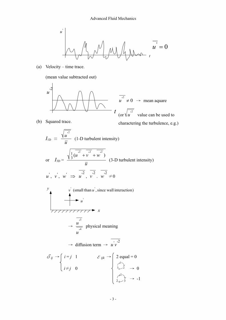
Advanced Fluid Mechanics
- 3 -
1
23
1
2 3
'u
t
0' =u
(a) Velocity – time trace.
(mean value subtracted out)
2'u
t (b) Squared trace.
I1D ≡ uu
2' (1-D turbulent intensity)
or I3D = u
wvu )(222 '''
31 ++
(3-D turbulent intensity)
'u , 'v , 'w ⇒ 2'u ,
2'v . 2'w ≠0
y
x
'u
'v )ninteractio wallsince , than small( 'u
→ 4
3
'
'
u
u physical meaning
→ diffusion term → 2''vu
δij → i = j 1 εijk → 2 equal = 0
i≠j 0 → 0
→ -1
02' ≠u → mean aquare
(or2'u value can be used to
charactering the turbulence, e.g.)
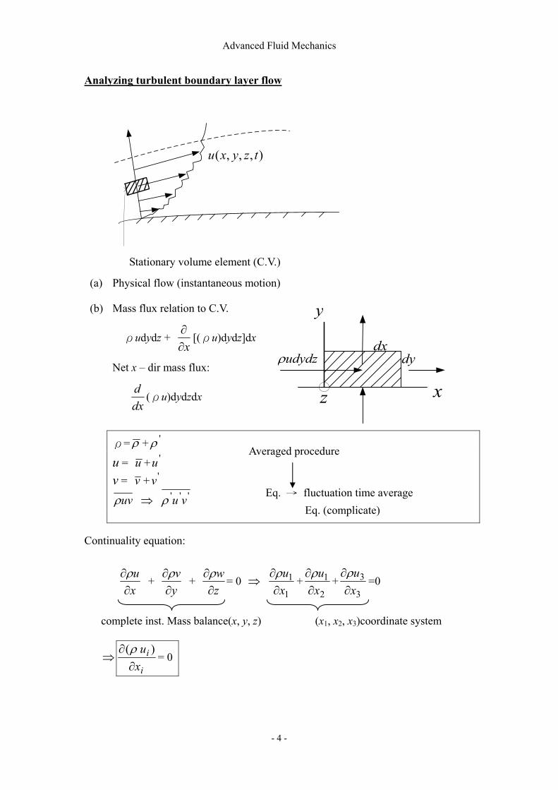
Advanced Fluid Mechanics
- 4 -
x
y
dxdyudydzρ
z
Analyzing turbulent boundary layer flow
),,,( tzyxu
Stationary volume element (C.V.)
(a) Physical flow (instantaneous motion)
(b) Mass flux relation to C.V.
ρudydz + x∂∂
[(ρu)dydz]dx
Net x – dir mass flux:
dxd
(ρu)dydzdx
ρ= ρ + 'ρ
u = u + 'u v = v + 'v
''' vuuv ρρ ⇒
Continuality equation:
xu
∂∂ρ
+ yv
∂∂ρ
+ zw
∂∂ρ
= 0 ⇒ 1
1xu
∂∂ρ
+2
1xu
∂∂ρ
+3
3xu
∂∂ρ
=0
complete inst. Mass balance(x, y, z) (x1, x2, x3)coordinate system
⇒i
ixu
∂∂ ) (ρ
= 0
Eq. → fluctuation time average Eq. (complicate)
Averaged procedure

Advanced Fluid Mechanics
- 5 -
Steady, Incompressible:
Mass flux consideration ⇒i
idxdu
=0 (1)
Momentum flux consideration
x
y
udydzρ
z
y
xz
),,,( tzyxu
dx
dy
dzuvdxdzy
uvdxdz )(ρρ∂∂
+
dxdydzux
dydzu )( 22 ρρ∂∂
+
uvdxdz)(ρ
(a) momentum fluxes
m& =ρAV
M =ρAV2 = ( m& )V
(b) pressure force
x
y
pdydz
z
dxpdydzx
pdydz )(∂∂
+
(c) viscous forces
x
y
dx
dydydzxu∂∂µ
dxdzyu∂∂µ
dxdydzxu
xdydz
xu )(
∂∂
∂∂
+∂∂ µµ
dxdydzxu
ydxdz
yu )(
∂∂
∂∂
+∂∂ µµ
yu
yx ∂∂
∝ µτ
Balance in x–dir:
x∂∂
(ρu2)(dxdydz) + y∂∂
(ρuv) (dxdydz) = xp∂∂
− (dxdydz) + µ ( 2
2
2
2
yu
xu
∂
∂+
∂
∂) (dxdydz)
Balance: Net Momentum efflux from
C.V. = sum of all ext. forces acting on fluid in C.V.
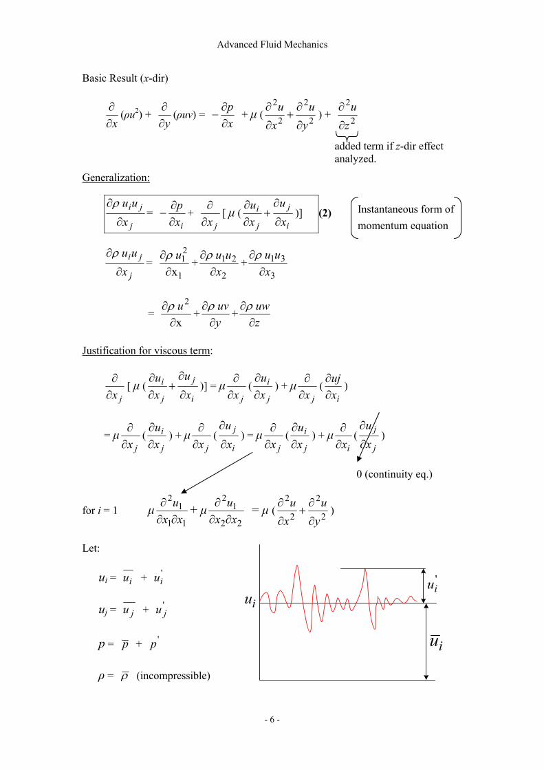
Advanced Fluid Mechanics
- 6 -
'iu
iu
iu
Basic Result (x-dir)
x∂∂
(ρu2) + y∂∂
(ρuv) = xp∂∂
− + µ ( 2
2
2
2
yu
xu
∂
∂+
∂
∂) + 2
2
zu
∂
∂
added term if z-dir effect analyzed.
Generalization:
j
ji
xuu
∂
∂ ρ=
ixp
∂∂
− + jx∂
∂[ µ (
i
j
j
ixu
xu
∂
∂+
∂∂
)] (2)
j
ji
xuu
∂
∂ ρ=
1
21
x
∂∂ uρ
+2
21 x
uu∂
∂ρ+
3
31 x
uu∂
∂ρ
= x 2
∂∂ uρ
+yuv
∂∂ ρ
+zuw∂
∂ ρ
Justification for viscous term:
jx∂∂
[ µ (i
j
j
ixu
xu
∂
∂+
∂∂
)] = µjx∂
∂(
j
ixu∂∂
) + µjx∂
∂(
ixuj∂∂
)
= µjx∂
∂(
j
ixu∂∂
) + µjx∂
∂(
i
j
xu∂
∂) = µ
jx∂∂
(j
ixu∂∂
) + µix∂∂
(j
j
xu∂
∂)
0 (continuity eq.)
for i = 1 µ11
12
xxu∂∂
∂ + µ22
12
xxu∂∂
∂ = µ ( 2
2
2
2
yu
xu
∂
∂+
∂
∂)
Let:
ui = iu + 'iu
uj = ju + 'ju
p = p + 'p
ρ = ρ (incompressible)
Instantaneous form of momentum equation
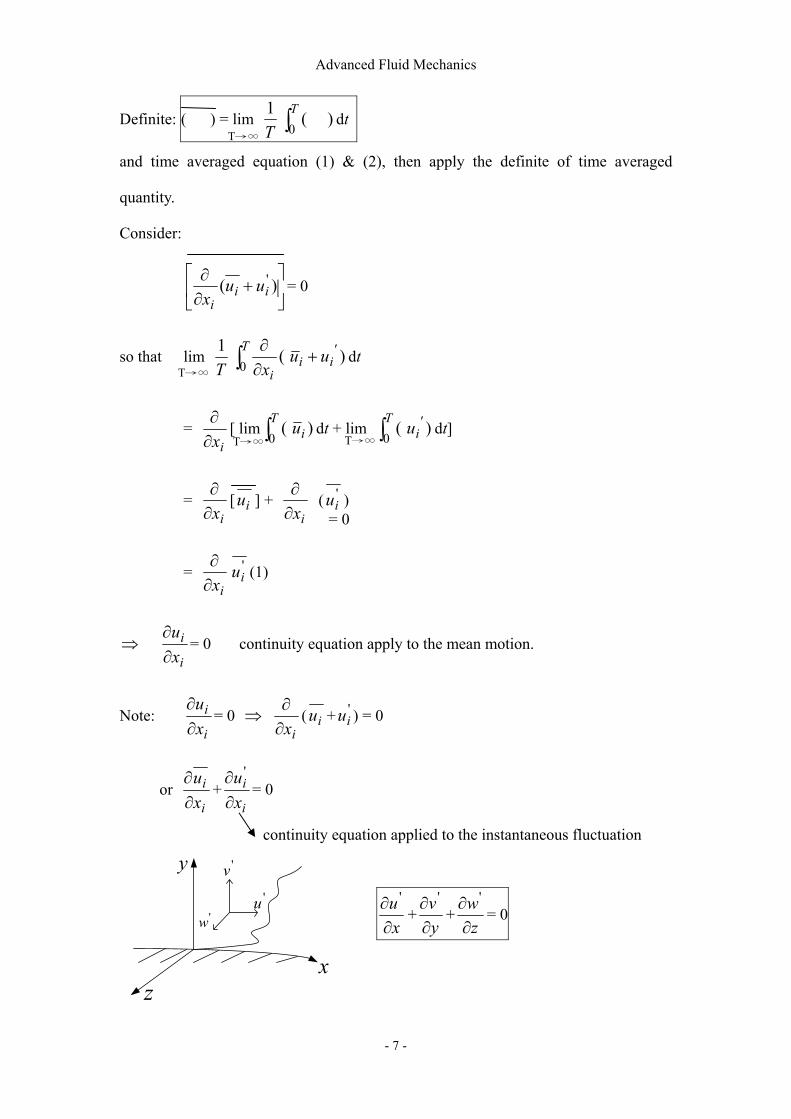
Advanced Fluid Mechanics
- 7 -
Definite: ( ) = lim T1∫
T0
) ( dt
and time averaged equation (1) & (2), then apply the definite of time averaged
quantity.
Consider:
+
∂∂ )( '
iii
uux
= 0
so that lim T1 )(
0∫ +∂∂T '
iii
uu x
dt
= ix∂∂
[ lim )(0∫T
iu dt + lim )(0∫T '
i u dt]
= ix∂∂
[ iu ] + ix∂∂
( 'iu )
= ix∂∂ '
iu (1)
⇒ i
ixu∂∂
= 0 continuity equation apply to the mean motion.
Note: i
ixu∂∂
= 0 ⇒ ix∂∂
( iu + 'iu ) = 0
or i
ixu∂∂
+i
ixu∂∂ '
= 0
continuity equation applied to the instantaneous fluctuation
x
y
z
'v'u
'w
T→∞
T→∞
T→∞ T→∞
= 0
xu∂∂ '
+yv∂∂ '
+z
w∂∂ '
= 0
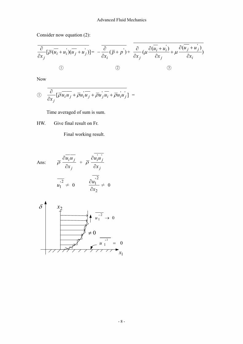
Advanced Fluid Mechanics
- 8 -
Consider now equation (2):
]))(([ ''jjii
juuuu
x++
∂∂ ρ = )( 'pp
xi+
∂∂
− + ))()(
(''
i
jj
j
ii
j xuu
xuu
x ∂
+∂+
∂+∂
∂∂ µµ
1 2 3
Now
1 ][ ''''jiijjiji
juuuuuuuu
xρρρρ +++
∂∂
=
Time averaged of sum is sum.
HW. Give final result on Fr.
Final working result.
Ans: ρj
ji
xuu
∂
∂ + ρ
j
ji
xuu
∂
∂ ''
2'
1u ≠ 0 2
2'1
xu∂∂
≠ 0
2x
1x
0≠
δ
02'
1 →u
02'
1 =u
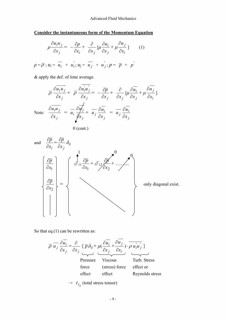
Advanced Fluid Mechanics
- 9 -
Consider the instantaneous form of the Momentum Equation
ρj
ji
xuu
∂
∂=
ixp
∂∂
− + jx∂
∂[µ
j
ixu∂∂ + µ
i
j
xu∂
∂] (1)
ρ = ρ ; ui = iu + 'iu ; uj = ju + '
ju ; p = p + 'p
& apply the def. of time average.
ρj
ji
xuu
∂
∂+ ρ
j
ji
xuu
∂
∂ ''=
jxp
∂∂
− + jx∂
∂[µ
j
ixu
∂∂ + µ
i
j
xu∂
∂]
Note: j
ji
xuu
∂
∂ = iu
j
j
xu∂
∂+ ju
j
ixu
∂∂ = ju
j
ixu
∂∂
0 (cont.)
and ix
p∂∂ =
jxp
∂∂ δij
1xp
∂∂ δ11
1xp
∂∂ +δ12
2xp
∂∂ + ……..
2xp
∂∂ = only diagonal exist.
So that eq.(1) can be rewritten as:
ρ juj
ixu
∂∂ =
jx∂∂ p δij + µ(
j
ixu
∂∂ +
i
j
xu∂
∂)- '' jiuuρ
→ ijtτ (total stress tensor)
001
Pressure force effect
Viscous (stress) force effect
Turb. Stress effect or Reynolds stress
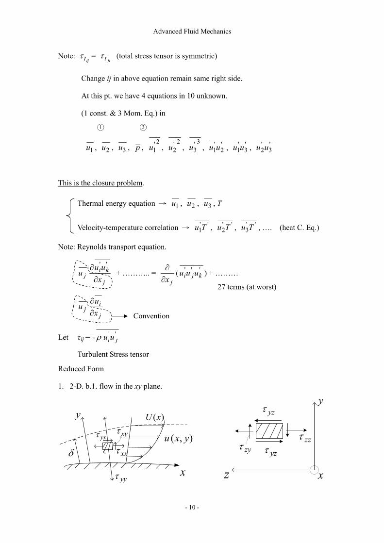
Advanced Fluid Mechanics
- 10 -
Note: ijtτ =
jitτ (total stress tensor is symmetric)
Change ij in above equation remain same right side.
At this pt. we have 4 equations in 10 unknown.
(1 const. & 3 Mom. Eq.) in
1 3
1u , 2u , 3u , p , 2'
1u , 2'
2u , 3'
3u , '2
'1uu , '
3'1uu , '
3'2uu
This is the closure problem.
Thermal energy equation → 1u , 2u , 3u , T
Velocity-temperature correlation → ''1Tu , ''
2Tu , ''3Tu , …. (heat C. Eq.)
Note: Reynolds transport equation.
juj
kixuu
∂∂ ''
+ ……….. = jx∂
∂( '''
kji uuu ) + ………
juj
ixu
∂∂
Let τij = - '' jiuuρ
Turbulent Stress tensor
Reduced Form
1. 2-D. b.1. flow in the xy plane.
yxτ
xxτ
xyτ
δ
x
y )(xU
),( yxu
yyτ x
y
z
yzτ
yzτzyτzzτ
27 terms (at worst)
Convention
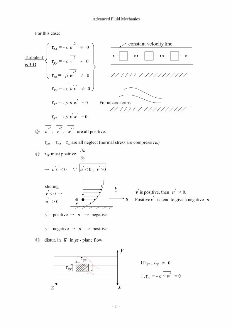
Advanced Fluid Mechanics
- 11 -
lineelocity constant v
termsunzeroFor
'u
'v
For this case:
τxx = -ρ2'u ≠ 0
τyy = -ρ2'v ≠ 0
τzz = -ρ2'w ≠ 0
τxy = -ρ ''vu ≠ 0
τxz = -ρ ''wu = 0
τyz = -ρ ''wv = 0
2'u ,
2'v , 3'w are all positive.
τxx, τyy, τzz are all neglect (normal stress are compressive.)
τxy must positive. yu∂∂
→ ''vu < 0 ∵ 'u < 0 ; 'v >0
'v = positive → 'u → negative
'v = negative → 'u → positive
distur. in u in yz - plane flow
yzτ
zyτ
y
z x
Turbulent is 3-D
slicting 'v < 0 → 'u > 0
'v is positive, then 'u < 0. Positive 'v is tend to give a negative 'u
If τyz , τzy ≠ 0
∴τyz = -ρ ''wv = 0
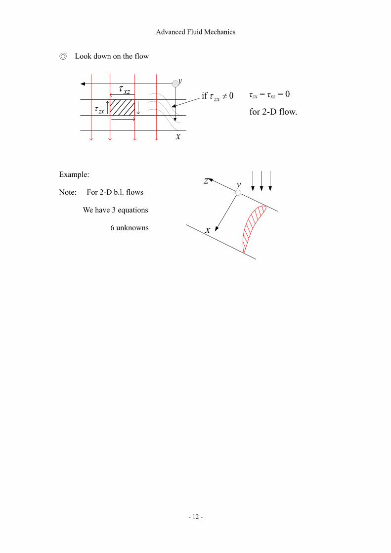
Advanced Fluid Mechanics
- 12 -
z
x
y
Look down on the flow
xzτ
zxτ
y
x
0 if ≠zxτ
Example:
Note: For 2-D b.l. flows
We have 3 equations
6 unknowns
τzx = τxz = 0
for 2-D flow.
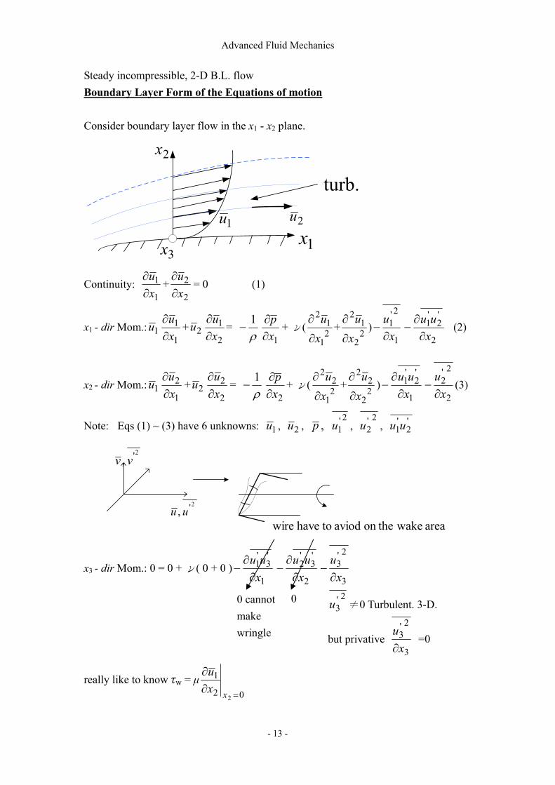
Advanced Fluid Mechanics
- 13 -
Steady incompressible, 2-D B.L. flow Boundary Layer Form of the Equations of motion Consider boundary layer flow in the x1 - x2 plane.
2x
1x3x
1u 2u
turb.
Continuity: 1
1xu∂∂
+2
2xu∂∂
= 0 (1)
x1 - dir Mom.: 1u1
1xu∂∂
+ 2u2
1xu∂∂
= ρ1
−1xp
∂∂
+ ν( 21
12
xu
∂
∂+ 2
2
12
xu
∂
∂)
1
2'1x
u∂
−2
'2
'1xuu
∂∂
− (2)
x2 - dir Mom.: 1u1
2xu∂∂
+ 2u2
2xu∂∂
= ρ1
−2xp
∂∂
+ ν( 21
22
xu
∂
∂+ 2
2
22
xu
∂
∂)
1
'2
'1xuu
∂∂
−2
2'2x
u∂
− (3)
Note: Eqs (1) ~ (3) have 6 unknowns: 1u , 2u , p , 2'
1u , 2'
2u , '2
'1uu
2' , uu
2' , vv
area wakeon the aviod tohave wire
x3 - dir Mom.: 0 = 0 + ν( 0 + 0 )1
'3
'1xuu
∂∂
−2
'3
'2xuu
∂∂
−3
2'3x
u∂
−
0
really like to know τw = µ02
1
2 =∂∂
xxu
0 cannot make wringle
2'3u ≠0 Turbulent. 3-D.
but privative 3
2'3x
u∂
=0

Advanced Fluid Mechanics
- 14 -
Cannot get 02
1
=∂∂
xxu
, unless solve the flow field.
(We need 3 additional equations to effect closure.)
Order – of – magnitude consideration
Let: 1. L1 & L2 be length scales in the x1 & x2 dir. respectively, (L1~x1 & L2 ~δ)
⇒ L2 << L1.
1x2x
)( 1x<<δs
.separation unlessthin,islayer boundary
here. know tohave typeEliptic
2. u1 & u2 be velocity scales in the x1 & x2 dir. Respectively.
3. V2 be the velocity scale of each RS comp.
( ''jiuu )
τij = -ρ ''jiuu
By correlation: ''jiuu ≡ ”stress” tensor (Kinematics sense)
(Verifiable experimentally)
0
1δy
2u
2v
2w
uv
0
Total stress tensor
Reynolds stress tensor

Advanced Fluid Mechanics
- 15 -
Justification (cross – derivation term)
Assume that
)(1
1
1xUu
= n
xx
1
1
2)(
δ
(a) Laminar case
∞U
1u
prescribed
1x
2x
)( 1xU∞
solution flow potential
*δ
shapebody erecalculat
∞U
do potential calculation on the original body.
n = 0.5 parabolic )(1
1
1xUu
= 2
1
2)(
x
xδ
(b) Turbulent flow
T
1x
2x
( η ≤ n ≤ 12) power law.
)(1
1
1xUu
= 71
1
2)(
x
xδ
~ 121