advanced analysis of resins production using …...advanced analysis of resins production using mvda...
TRANSCRIPT
Advanced analysis of resins production using MVDA tools
Clara de Castro Nemésio
Thesis to obtain the Master of Science Degree in
Chemical Engineering
Supervisors:
Doutora Engenheira Vera Mónica de Campos Loures Lourenço
Professor Doutor José Monteiro Cardoso de Menezes
Examination Committee
Chairperson: Prof. Doutora Benilde de Jesus Vieira Saramago
Supervisor: Prof. Doutor José Monteiro Cardoso de Menezes
Members of the Committee: Prof. Doutora Maria Joana Castelo Branco de Assis
Teixeira Neiva Correia
November 2016


iii
Acknowledgments
This thesis was one of the best experiences I have ever had and it was an amazing challenge. It required
me to change to a foreign country with a different culture and a very difficult language. Now I can say it
was the fastest however it was the best decision I could have ever made. But this challenge would not
be surpassed without help and I must thank the people that made it possible. The main responsible for
this adventure was without doubt my supervisor at my university, Professor Doutor José Cardoso de
Menezes, who made it possible! Without his persistency to find me and introducing me to Doutora Vera
Lourenço who was at that time in Portugal I would not be here. I have to thank him for giving me this
opportunity, for his scientific supervision and suggestions, friendship and patience. Without him nothing
would have been possible! The other person without whom I would not have had this opportunity was
Doutora Vera Lourenço, my supervisor at Trespa. To her I owe the conditions I was provided with in this
work, without her project proposal nothing would have happened. I want to thank her for her excellent
supervision, the patience and availability with all the questions I had, sometimes it was certainly
overwhelming. I want to thank her for all the understanding and scientific supervision. It was a
tremendous pleasure to meet and work with her, besides a supervisor I won an excellent friend that I
will never forget and thank enough. Also, a special acknowledgement to Doutor Pedro Mena, my second
supervisor at Trespa, for the support after Doutora Vera Lourenço had her maternity leave. I have to
thank for all the constructive criticism, friendship, knowledge about the production process and for his
trust in my work. At Trespa there were many people who were always available to help me with all the
questions. Pattiya, thank you for all the companionship at home and for the help when I was struggling
with the endless excel sheets. Thank you all for all the support! Finally, I have to thank the ones that did
not have anything to do with Trespa but gave the emotional support. To my parents for allowing me to
have this opportunity that changed my life, thank you for helping me settle down and for all the wise
advices. They know how much they mean and are important. To my brother for all his scientific
knowledge, for his help with the English, his support, happiness and the visit. A special thanks to him
and Ana for being the ones that said I should not miss this life opportunity, thank you. To my boyfriend
Konrad, whom I met during my stay here, thank you for all the patience when I was struggling with the
project, all the love. Without your support when I was missing home I think I would not have made it in
this country that I ended up liking a lot. Thank you for all your kindness and now we have a big challenge
ahead but I believe we will make it! To my friends the ones that came to visit me and the ones that
wanted and were not able to. You all know how important you are for me. A special thanks to Rita and
Patricia, for all the friendship since the beginning of our journey at Técnico, for all the support with the
bureaucracy with the thesis and the knowledge and specially for the friendship and personal advices.
Thank you for your visit, you are my friends for life and you know it!

v
Resumo
Foi realizado o estudo de um processo industrial de produção de resinas para avaliar o impacto da
qualidade das matérias-primas (através da análise de espectros FT-IR) e do processo de fabrico na
qualidade final da resina, obtida por espectroscopia de infravermelho próximo (NIR). O objetivo do
estudo foi aumentar o conhecimento do processo de produção de forma a identificar os aspetos críticos
para a qualidade das resinas.
O estudo iniciou-se com a análise multivariada (MVDA) dos diferentes conjuntos de dados (matérias-
primas, resinas e processo) de forma a conhecer o processo e descobrir os aspetos críticos.
Numa segunda fase, propriedades físicas e químicas das resinas foram medidas em laboratório de
forma a dar um significado físico aos espectros colhidos por NIR. Verificaram-se diferenças nas
propriedades das resinas consoante o reator onde são produzidas.
A avaliação do processo de produção mostrou que a eficiência do sistema de refrigeração aquando da
produção da resina é um aspeto crítico para a qualidade final da mesma, assim como o reator onde
são produzidas.
Por último, foi possível relacionar a análise aos espectros colhidos por NIR com as análises de
laboratório. Esta relação permitirá, futuramente, desenvolver um novo controlo de qualidade para a
empresa, complementar ou mesmo substituto do atual.
Palavras-chave:
Resina, MVDA, NIR, FT-IR, garantia de qualidade, processo de produção.
Por motivos de confidencialidade, os fornecedores de matérias-primas foram omitidos, assim
como valores de processo e às análises de laboratório foram dadas unidades arbitrárias.

vii
Abstract
A study was conducted on an industrial process of resins production to evaluate the impact of raw
materials quality (analysed by FT-IR spectra) and the manufacturing process in the resins final quality,
obtained by near infrared spectroscopy (NIR). The objective was to increase the knowledge of the
production process in order to identify critical aspects for resins quality.
The first step was multivariate analysis (MVDA) of different datasets (raw materials, resins and process)
in order to increase the production process knowledge and identify its critical aspects.
In the second step, chemical and physical properties of the resins were measured in the lab in order to
give a physical meaning to the NIR spectra. The resins show different properties according to the reactor
where they are produced.
The production process analysis showed that the cooling system’s efficiency is a critical aspect for the
final quality of the resin as well as the reactor where the resin is produced.
Finally, it was possible to correlate the spectral analysis of the NIR with the lab analyses. This correlation
will allow in the future to develop a quality control for Trespa to replace the currently installed.
Key words:
Resin, MVDA, NIR, FT-IR, quality assurance, production process.
For confidentiality reasons, the raw materials suppliers have been omitted, as well as process
values and the laboratory analyses have been given arbitrary units.

ix
Index
Acknowledgments ................................................................................................................................... iii
Resumo ....................................................................................................................................................v
Abstract................................................................................................................................................... vii
Index ........................................................................................................................................................ ix
List of figures ........................................................................................................................................... xi
List of Tables .......................................................................................................................................... xv
List of symbols and abbreviations ........................................................................................................ xvii
Part A. - Introduction .......................................................................................................................... 1
Chapter I. - Trespa International B.V.: overview............................................................................. 1
1. - Context ................................................................................................................................ 1
2. - Trespa’s products ................................................................................................................ 1
3. - Production process of the panels ........................................................................................ 2
Chapter II. - Objectives and Thesis Structure .................................................................................. 3
1. - Objectives ............................................................................................................................ 3
2. - Thesis Structure................................................................................................................... 3
Chapter III. - Resin production .......................................................................................................... 5
1. - Reactors Design .................................................................................................................. 5
2. - Reaction Mechanism ........................................................................................................... 7
3. - Reaction Path ...................................................................................................................... 9
Chapter IV. - Multivariate Data Analysis (MVDA) ....................................................................... 11
1. - Chemometrics .................................................................................................................... 11
2. - Signal (pre-)processing ..................................................................................................... 12
3. - Principal Components Analysis (PCA) .............................................................................. 13
4. - Partial Least Squares (PLS) .............................................................................................. 15
5. - Batch Modelling ................................................................................................................. 15
Chapter V. - Vibrational spectroscopies ......................................................................................... 17
Chapter VI. - Physical and chemical characterisation of resins .................................................. 19
Part B. - Results and Discussion ..................................................................................................... 21
x
Chapter I. - Study of raw materials variability ............................................................................... 21
1. - Phenol ................................................................................................................................ 21
2. - Formaldehyde .................................................................................................................... 25
3. - Catalyst .............................................................................................................................. 28
4. - Other raw materials ........................................................................................................... 29
5. - Conclusions ....................................................................................................................... 34
Chapter II. - Assessment of the quality for B13 resin .................................................................... 35
1. - Variability of resin quality by NIR spectral analysis ........................................................... 35
2. - Production process path .................................................................................................... 42
3. - Process versus resin quality (data integration) ................................................................. 52
4. - Conclusions ....................................................................................................................... 57
Chapter III. - Assessment of the quality for B52 resin .................................................................... 59
1. - Variability of resin quality by NIR spectral analysis ........................................................... 59
2. - Production process path .................................................................................................... 62
3. - Process versus resin quality (data integration) ................................................................. 66
4. - Conclusions ....................................................................................................................... 70
Chapter IV. - Conclusions and future work ................................................................................. 71
1. - Conclusions ....................................................................................................................... 71
2. - Future Work ....................................................................................................................... 72
References ............................................................................................................................................ 73
Appendices ............................................................................................................................................ 75
Appendix A: Univariate statistical process control charts B13 resin batches .................................... 75
Appendix B: Univariate statistical process control charts B52 resin batches .................................... 76
xi
List of figures
Figure 1 - Layers of a Trespa panel. ....................................................................................................... 1
Figure 2 - Production process of Trespa's HPL. ..................................................................................... 2
Figure 3 - Reactors design scheme. [2] .................................................................................................. 6
Figure 4 - Activation of phenol by deprotonation and aromatic electrophilic substitution. [3] ................. 8
Figure 5 - Example of a resol, phenolic resin. [4] .................................................................................... 8
Figure 6 - Schematic representation of Chemometrics fields of application. ........................................ 12
Figure 7 - Raw (a) and first derivative pre-processed (b) NIR spectra. ................................................ 13
Figure 8 - Example of scores and loadings plots [11] ........................................................................... 14
Figure 9 - Three-way table of batch process data. ................................................................................ 16
Figure 10 – Multivariate control chart of three batches. ........................................................................ 16
Figure 11 – FT-IR (a) and NIR (b) spectrometers. ............................................................................... 17
Figure 12 – FT-IR and NIR vibrational levels. [13] ................................................................................ 18
Figure 13 - Phenol raw (left side) and pre-treated (right side) spectra. ................................................ 22
Figure 14 - Reference spectra for both suppliers, A and B. .................................................................. 22
Figure 15 - Scores plot of PCA model for pure phenol, coloured by year (left side) and supplier (right
side). ...................................................................................................................................................... 23
Figure 16 – 80% phenolic compounds solution raw (left side) and pre-treated (right side) spectra. .... 23
Figure 17 - Scores plot of PCA model for 80% phenolic compounds solution, coloured by year (a) and
supplier (b) for the first and second PC. Scores plot for the first PC (c) according to the sampling. .... 24
Figure 18 - Scores plot for the first principal component for supplier C (a) and supplier D (b) according
to the sampling, coloured by year. ........................................................................................................ 25
Figure 19 - Raw spectra of formaldehyde solution. ............................................................................... 25
Figure 20 - Loadings plot of the first PCA model with the fingerprint for formaldehyde solution. PC1
coloured in blue and PC2 in green. ....................................................................................................... 26
Figure 21 - Scores plot for the second PCA model developed (without fingerprint) coloured by supplier
(a), year (b). Scores plot for the first (c) and second (d) PC along time, coloured by year. .................. 27
Figure 22 - Spectra from the truck (blue coloured) and the sampling arm (red coloured). ................... 27
Figure 23 - Catalyst raw (left side) and pre-treated (right side) spectra. ............................................... 28
Figure 24 - Scores plot of the catalyst PCA model (a) and scores plot for the first principal component
according to the sampling (b), coloured by year. .................................................................................. 28
Figure 25 - Loadings plot of the PCA model for the basic catalyst solution. ......................................... 29
Figure 26 - Diluent raw (left side) and pre-treated spectra (right side). ................................................ 30
Figure 27 - Scores plot of the diluent, coloured by years. .................................................................... 30
Figure 28 - Raw (left side) and pre-treated (right side) spectra of the plasticizer ................................. 31
Figure 29 - Scores plot of the PCA model for the plasticizer. ............................................................... 31
Figure 30 - Raw (left side) and pre-treated (right side) of the fire retardant agent A. ........................... 32
Figure 31 - Scores plot of the PCA model developed for the fire retardant agent A. ............................ 32
Figure 32 - Raw (left side) and pre-processed (right side) spectra of the fire retardant agent B. ......... 33
Figure 33 - Scores plot of the fire retardant agent B, coloured by year. ............................................... 33
xii
Figure 34 - Raw spectra of B13 resins produced during six months. ................................................... 35
Figure 35 - Values of Q2 (cumulative) with the number of PC. ............................................................. 36
Figure 36 - Pre-processed spectra, with SNV method, for B13 resin. .................................................. 36
Figure 37 - Scores plot of the PCA model developed for B13 resin, coloured by reactors (left side) and
phenol suppliers (right side). ................................................................................................................. 37
Figure 38 - Outliers A, B (Left side) and C (Right side) comparedwith an average spectra. ................ 38
Figure 39 – Spectra of bands 1 (a), 2 (c) and 3 (e) and scores plot for the correspondent developed
models for band 1 (b), band 2 (d) and band 3 (f), coloured by reactor. ................................................ 39
Figure 40 - p[n] for the nth PC versus wavenumber............................................................................... 40
Figure 41 - Intensity of the 5970 cm-1 wavenumber in the scores plot of the PCA model for band 1. .. 41
Figure 42 – Typical temperature profiles inside the reactors. ............................................................... 43
Figure 43 – Batch level modelling: Scores plot for the PCA model (a) and source of variations plot (b)
with the three reactors. .......................................................................................................................... 43
Figure 44 - Scores plots for phase 1(left side) and phase 2 (right side) of the process in reactor 5
coloured according to time maturity in minutes (batch starts in blue and ends in red). ........................ 45
Figure 45 - Scores plots for the different reactors in the 3rd phase of the process: (a) reactor 3, (b) reactor
4 and (c) reactor 5. The scores are coloured according to batch maturity time in minutes (batch starts in
blue, evolves to green and ends in red). ............................................................................................... 45
Figure 46 - Loadings plot for phase 1 (left side), phase 2 (centre) and phase 3 (right side) for reactor 5.
............................................................................................................................................................... 46
Figure 47 - Multivariate batch control chart for the third phase of reactor 5 (a) and temperature profile
during the 3rd phase. Batches are coloured according to the production month. Thick green dashed line:
average temperature profile, thick red dashed lines: batch control chart limits for the temperature. On
chart (a) the solid lines correspond to the scores of the 1st LV and on (b) it is the temperature each
minute for the third phase. ..................................................................................................................... 46
Figure 48 - Batch level modelling for reactor 3: Scores plot in which each dot corresponds to one whole
batch, coloured by week (left side) and sources of variation plot (right side) for all three phases. ....... 47
Figure 49 - Batch level modelling for reactor 3: Scores plot with the relevant weeks. .......................... 47
Figure 50 - Variable batch control chart: Water flow of the condenser (a) and vapour temperature (b)
during the third phase for reactor 3. Batches are coloured per week: Week 9 blue coloured and week
15 purple coloured. ................................................................................................................................ 48
Figure 51 - Loadings plot for the observation level of the third phase of reactor 3. .............................. 48
Figure 52 - Variable batch control chart: Water flow of the condenser (a) and vapour temperature (b)
during the third phase for reactor 3. Batches are coloured per week: Week 3 orange coloured and week
6 red coloured. ....................................................................................................................................... 49
Figure 53 - Batch level modelling for reactor 4: Scores plot in which each dot corresponds to one whole
batch, coloured by duration of the third phase (left side) and sources of variation plot (right side) for all
three phases. ......................................................................................................................................... 50
Figure 54 - Batch level modelling for reactor 4: Scores plot with the relevant weeks. .......................... 50
xiii
Figure 55 - Variable batch control charts: Temperature inside the reactor (a); Cooling coil flow rate (b);
Flow of the condenser (c); and vapour temperature (d) during the third phase for reactor 4. Batches are
coloured per week: Week 9 blue coloured and week 15 purple coloured. ............................................ 51
Figure 56 - Outliers flow in the condenser compared to the average for the third phase in reactor 4. . 51
Figure 57 - Batch level modelling for reactor 5: Scores plot of the first PCA model developed in which
each dot corresponds to one whole batch, coloured by month (a) and scores plot for the second PCA
model, excluding April, coloured by month (b). ..................................................................................... 52
Figure 58 - Scores plot of the developed PCA model for band 1 of the spectra coloured by molecular
weight. Blue corresponds to the lowest molecular weights and red to highest molecular weights. ...... 54
Figure 59 - Univariate statistical process control chart for the molecular weight of the 26 resin batches
analysed in the lab. The values of the molecular weights have arbitrary units due to confidentiality
purposes. ............................................................................................................................................... 54
Figure 60 - USPC chart for the phenol content of the 26 resin batches analysed in the lab. The values
of the phenol contents have arbitrary units due to confidentiality purposes. ........................................ 55
Figure 61 - PLS model: correlation between NIR spectra and molecular weight. Green: external
validation; Blue: calibration dataset. ...................................................................................................... 55
Figure 62 - Univariate statistical process control chart for curing time (left side) and viscosity (right side)
of the 26 resin batches analysed in the lab. The values shown have arbitrary units due to confidentiality
purposes. ............................................................................................................................................... 56
Figure 63 - Raw spectra (left side) and pre-processed with SNV (right side) of B52 resins produced
during six months. ................................................................................................................................. 59
Figure 64 - Scores plot (a) and loadings plot (b) for B52 resin produced in reactor 5. ......................... 60
Figure 65 - Scores plot of the PCA model developed for band 1 (left side) and band 3 (right side) for
B52 resin, coloured by supplier. ............................................................................................................ 61
Figure 66 - Spectra of band 1 (left side) and band 3 (right side) for B52 resin, coloured by supplier... 61
Figure 67 - Temperature profile inside reactor 5 for B52 resin. ............................................................ 62
Figure 68 - Scores plots for reactor 5 in the third phase of the process. The scores are coloured
according to the month where they were produced. ............................................................................. 63
Figure 69 - Batch control chart: Temperature inside the reactor batch control chart for phase 1 (left side)
and phase 3 (right side) for reactor 5. Batches are coloured according to the production month. Thick
green dashed line: average temperature profile, thick red dashed lines: batch control chart limits for the
temperature. .......................................................................................................................................... 64
Figure 70 - Batch level modelling for reactor 5: Scores plot coloured by supplier with the clusters
identified. ............................................................................................................................................... 65
Figure 71 - Variable batch control charts: Flow of the condenser for the clusters: Phase 1 (left side) and
Phase 3 (right side). Batches are coloured per month: April orange coloured and June blue coloured.
............................................................................................................................................................... 66
Figure 72 - PLS model: correlation between NIR spectra and free-phenol property for band 1. .......... 68
xiv
Figure 73 - Univariate statistical process control chart for molecular weight (left side) and Phenol content
(right side) of 18 resin batches analysed in the lab. The values shown have arbitrary units due to
confidentiality purposes. ........................................................................................................................ 69
Figure 74 - Univariate statistical process control chart for viscosity of 18 resin batches analysed in the
lab. The values shown have arbitrary units due to confidentiality purposes. ........................................ 69
Figure 75 - Univariate statistical process control chart for: (a) curing time and (b) active content of 18
resin batches analysed in the lab. The values shown have arbitrary units due to confidentiality purposes.
............................................................................................................................................................... 69
Figure A.1 - Univariate statistical process control chart for Formaldehyde content (left side) and pH (right
side) of 26 resin batches analysed in the lab. The values shown have arbitrary units due to confidentiality
purposes. ............................................................................................................................................... 75
Figure A.2 - Univariate statistical process control chart for Water tolerance (left side) and Active content
(right side) of 26 resin batches analysed in the lab. The values shown have arbitrary units due to
confidentiality purposes. ........................................................................................................................ 75
Figure B. 1 - Univariate statistical process control chart for formaldehyde (left side) and pH (right side)
of 18 resin batches analysed in the lab. The values shown have arbitrary units due to confidentiality
purposes. ............................................................................................................................................... 76
Figure B.2 - Univariate statistical process control chart for water tolerance of 18 resin batches analysed
in the lab. The values shown have arbitrary units due to confidentiality purposes. .............................. 76
xv
List of Tables
Table 1 - F-values for ANOVA test of the first PC (63.1% of explained variance), for a significance level
of 95%(α=0.05). ..................................................................................................................................... 37
Table 2 – Spectra PCA models indicators. Number of PC (PC), explained variance ( 𝑅𝒙𝟐), and variance
predicted by the model (Q2). .................................................................................................................. 39
Table 3 – Wavenumbers that dominate the PCA models. .................................................................... 40
Table 4 - Multiway PLS indicators for all the developed models. .......................................................... 44
Table 5 - Batch level PCA model indicators for reactor 3. .................................................................... 46
Table 6 - Batch level PCA model indicators for reactor 4. .................................................................... 49
Table 7 - Spectra PCA models indicators for reactor 5: Number of PC (PC), explained variance ( 𝑹𝒙𝟐),
and variance predicted by the model (Q2). ............................................................................................ 61
Table 8 - Multiway PLS indicators for developed model for reactor 5 in B52 resin............................... 63
Table 9 - Batch level PCA model indicators for reactor 5. .................................................................... 64

xvii
List of symbols and abbreviations
Symbols
p[n] – loading of nth principal component / latent variable
Q2 – total variance of the model
Abbreviations
BSPC – Batch Statistical Process Control
EBC – Electron Beam Curing
EN - European Norm
FT-IR – Fourier Transformed Infrared Spectroscopy
GPC – Gel Permeation Chromatography
HPL – High-Pressure Laminates
HPLC – High-Performance Liquid Chromatography
LV – Latent variables
MSC – Multiplicative Scatter Correction
MVDA – Multivariate Data Analysis
NIR – Near-infrared spectroscopy
NMR – Nuclear Molecular Resonance spectroscopy
PC – Principal Component
PCA – Principal Components Analysis
PLS – Partial Least Squares
SNV – Standard Normal Variate
USA – United States of America

1
Part A. - Introduction
This thesis is the result of an internship at Trespa International B.V in order to obtain a Master of Science
degree in Chemical Engineering. It took place from the 15th of February until the 28th of October of 2016.
Chapter I. - Trespa International B.V.: overview
1. - Context
Trespa International B.V. is a chemical company, founded in 1960, that produces High-Pressure
Laminates (HPL) panels for architectural purposes such as decorative façades and exterior cladding.
Trespa’s main focus is on developing their products with a combination of quality manufacturing
technologies and solutions for architectural applications. The company relies on these statements:
reliability, innovation, driven, durability, refreshing.
Trespa’s headquarters and the production plant are located in Weert (The Netherlands). The company
also has three design centres located in New York (USA), Barcelona (Spain) and Santiago (Chile). [1]
Trespa produced around 4 000 000 square meters of panels in 2015.
2. - Trespa’s products
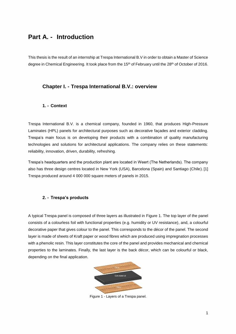
A typical Trespa panel is composed of three layers as illustrated in Figure 1. The top layer of the panel
consists of a colourless foil with functional properties (e.g. humidity or UV resistance), and, a colourful
decorative paper that gives colour to the panel. This corresponds to the décor of the panel. The second
layer is made of sheets of Kraft paper or wood fibres which are produced using impregnation processes
with a phenolic resin. This layer constitutes the core of the panel and provides mechanical and chemical
properties to the laminates. Finally, the last layer is the back décor, which can be colourful or black,
depending on the final application.
Figure 1 - Layers of a Trespa panel.
2
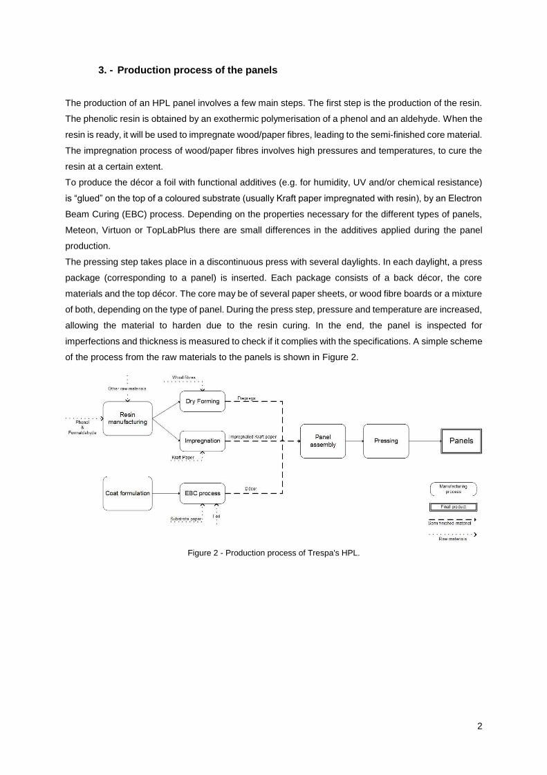
3. - Production process of the panels
The production of an HPL panel involves a few main steps. The first step is the production of the resin.
The phenolic resin is obtained by an exothermic polymerisation of a phenol and an aldehyde. When the
resin is ready, it will be used to impregnate wood/paper fibres, leading to the semi-finished core material.
The impregnation process of wood/paper fibres involves high pressures and temperatures, to cure the
resin at a certain extent.
To produce the décor a foil with functional additives (e.g. for humidity, UV and/or chemical resistance)
is “glued” on the top of a coloured substrate (usually Kraft paper impregnated with resin), by an Electron
Beam Curing (EBC) process. Depending on the properties necessary for the different types of panels,
Meteon, Virtuon or TopLabPlus there are small differences in the additives applied during the panel
production.
The pressing step takes place in a discontinuous press with several daylights. In each daylight, a press
package (corresponding to a panel) is inserted. Each package consists of a back décor, the core
materials and the top décor. The core may be of several paper sheets, or wood fibre boards or a mixture
of both, depending on the type of panel. During the press step, pressure and temperature are increased,
allowing the material to harden due to the resin curing. In the end, the panel is inspected for
imperfections and thickness is measured to check if it complies with the specifications. A simple scheme
of the process from the raw materials to the panels is shown in Figure 2.
Figure 2 - Production process of Trespa's HPL.
3
Chapter II. - Objectives and Thesis Structure
1. - Objectives
The main objective of this project is to increase the understanding of the resin manufacturing process
in order to identify the main critical aspects for the resin quality. These can be related to raw materials
quality or process path of resins production. The followed approach was: 1) to detect and check process
variability and identify trends taking into account seasonality effects, suppliers of the raw materials or
even the reactors where the resins are produced; 2) to analyse the quality of the resins using collected
near- infrared (NIR) spectra searching for differences between the reactors and also seasonality effects;
3) to execute lab analyses to selected resin batches in order to give a physical meaning to the NIR
spectral analysis and to better understand their quality variations; 4) to integrate the different types of
data (NIR spectra, lab results and process data) in order to check what has more influence in the quality
of the resin (Quality Assurance).
2. - Thesis Structure
This thesis is divided into two parts, Part A and B. Part A gives an overview of the main aspects
concerning the realization of this project. Part B describes the approach to achieve the project
objectives.
In Part A, Chapter I gives an overview of Trespa International B.V., describing its products and the
production process of the panels. Chapter II describes the objectives of this project. Chapter III is
focused on describing resins production from the reactors design and constitution until the reaction path
to obtain a resin. Chapter IV is dedicated to explain the MVDA techniques used throughout the project.
Chapter V gives a brief explanation of the vibrational spectroscopies used in the raw materials and
resins study. Lastly, Chapter VI is about physical and chemical characterisation of resins, performed in
the lab and that allowed to give a physical/chemical meaning to the MVDA techniques.
In Part B, for Chapter I the stored spectra for the raw materials is studied with MVDA techniques, to
identify differences between the suppliers and quality variability of the raw materials. Chapters II and III
describe all the analyses performed for B13 and B52 resins, respectively. In these Chapters the
approach is the same. Analysis of the NIR spectra, using MVDA techniques is performed in order to
analyse the quality of the resin given by spectral analysis. Historical process data concerning the resin
production process is analysed using MVDA techniques to identify critical aspects for process quality.
Integration of all the data in order to see common patterns in the NIR spectral analysis and the process
was performed in the end of each Chapter (II for B13 and III for B52). Finally, in Chapter IV of Part B. -
conclusions are presented and suggestions of future work are made, indicating where there is still room
for further improvement.

5
Chapter III. - Resin production
The project that originated this thesis was more focused on the resin production which is the first step
of the production process of a Trespa panel. A resin is a synthetic polymer that is formed during the
reaction between an aldehyde and phenol.
Currently, there are eight different resin formulations produced at Trespa with differences in the raw
materials ratios and additives that will provide additional properties to the resins and consequently to
the laminates. In this project, B13, B25, and B52 were analysed, being B13 and B25 standard resins,
and B52 a post-forming resin. The main difference between B13 and B25 is that the first is used for
impregnation with Kraft paper and the second for impregnation with wood fibres. The resin production
process may be crucial to the quality of a panel since this semi-finished material accounts partially for
the chemical and mechanical properties of the final panel.
1. - Reactors Design
The phenolic resins are produced in three different reactors available at the resin tower: reactors 3, 4
and 5. Those reactors have some differences that will be described below.
All three reactors are constituted by:
Reactor vessel;
Heat storage for emergency situations;
Dosing system for the catalyst;
Riser tube;
Condenser;
Distillation vessel;
Vacuum unit (only for reactor 5).
The reactor vessel is where the raw materials are loaded and where the reaction occurs, being the most
important part of the reactors. The bottom and the walls of all three reactors have insulation to ensure
that the heat inside the reactor does not have any external influence. Reactors 3 and 4 have a capacity
of 5,5 ton, each, and reactor 5 has a capacity of 6 ton. Each reactor has an agitator, cooling and heating
coils and pressure and temperature monitoring systems.
All raw materials are introduced through the upper inlet of the reactor vessel and the agitator ensures
that the mixing of the raw materials is efficient and that the heat circulation is properly distributed. Along
the wall of the reactor vessels, showed in Figure 3, there is a spiral that corresponds to the cooling coil
in which there is cooling water circulating. The water is introduced in the lower inlet of the cooling coil
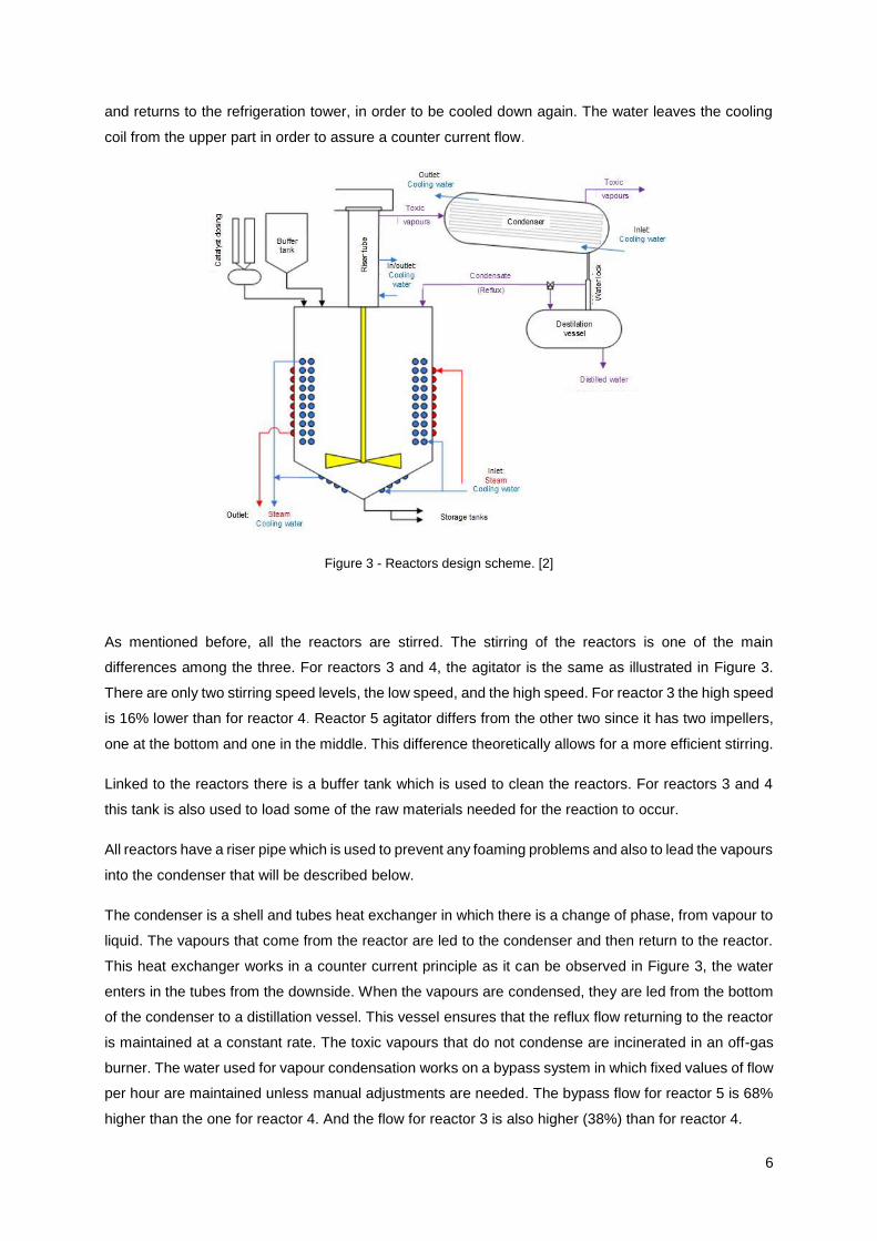
6
and returns to the refrigeration tower, in order to be cooled down again. The water leaves the cooling
coil from the upper part in order to assure a counter current flow.
Figure 3 - Reactors design scheme. [2]
As mentioned before, all the reactors are stirred. The stirring of the reactors is one of the main
differences among the three. For reactors 3 and 4, the agitator is the same as illustrated in Figure 3.
There are only two stirring speed levels, the low speed, and the high speed. For reactor 3 the high speed
is 16% lower than for reactor 4. Reactor 5 agitator differs from the other two since it has two impellers,
one at the bottom and one in the middle. This difference theoretically allows for a more efficient stirring.
Linked to the reactors there is a buffer tank which is used to clean the reactors. For reactors 3 and 4
this tank is also used to load some of the raw materials needed for the reaction to occur.
All reactors have a riser pipe which is used to prevent any foaming problems and also to lead the vapours
into the condenser that will be described below.
The condenser is a shell and tubes heat exchanger in which there is a change of phase, from vapour to
liquid. The vapours that come from the reactor are led to the condenser and then return to the reactor.
This heat exchanger works in a counter current principle as it can be observed in Figure 3, the water
enters in the tubes from the downside. When the vapours are condensed, they are led from the bottom
of the condenser to a distillation vessel. This vessel ensures that the reflux flow returning to the reactor
is maintained at a constant rate. The toxic vapours that do not condense are incinerated in an off-gas
burner. The water used for vapour condensation works on a bypass system in which fixed values of flow
per hour are maintained unless manual adjustments are needed. The bypass flow for reactor 5 is 68%
higher than the one for reactor 4. And the flow for reactor 3 is also higher (38%) than for reactor 4.
7
In the distillation vessel, there is a water trap that ensures that no vapours from the reactor enter these
pipelines. At the end of each batch what is still inside the distillation vessel is led to a process tank for
posterior reutilization.
The major difference between reactor 5 and reactors 3 and 4 is that the previous has a vacuum system.
This vacuum system is only used during the cooling phase. Because of this vacuum system the cooling
phase in reactor 5 is 20% faster than in the other two. The vacuum system of reactor 5 is constituted by
a vacuum pump, a buffer tank for the water that circulates in the vacuum pump, and a heater for the
water.
To finalise the description of the reactors design it is important to explain how the control of the
temperature is executed. The temperature inside the reactor is the controlled variable and the
manipulated is the flow of the cooling water that enters in the cooling coils. The flow of the cooling water
ensures that the temperature is maintained at the reflux temperature, during the reaction phase.
Runaway conditions and safety issues are assured with this type of control. In general, chemical
industries have very complex controlling systems. However, for this project the most important one is
the temperature control.
2. - Reaction Mechanism
The phenolic resins can be of two different types: novolacs and resols that are formed by a step-growth
polymerisation reaction. For the resols polycondensation occurs with a basic catalyst and the functional
groups are the hydroxymethyl groups and the dimethylene ether bridge. These two are reactive groups.
In order to limit the growth of the polymer in these resins, a substoichiometric amount of the aldehydes
that are added into the reaction mixture is used. [3]
The resins produced at Trespa are the resols type and the raw materials used are formaldehyde, phenol
and also a basic catalyst.
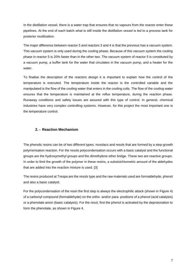
For the polycondensation of the resin the first step is always the electrophilic attack (shown in Figure 4)
of a carbonyl compound (formaldehyde) on the ortho- and/or para- positions of a phenol (acid catalysis)
or a phenolate anion (basic catalysis). For the resol, first the phenol is activated by the deprotonation to
form the phenolate, as shown in Figure 4.
8
Figure 4 - Activation of phenol by deprotonation and aromatic electrophilic substitution. [3]
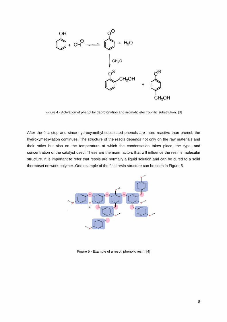
After the first step and since hydroxymethyl-substituted phenols are more reactive than phenol, the
hydroxymethylation continues. The structure of the resols depends not only on the raw materials and
their ratios but also on the temperature at which the condensation takes place, the type, and
concentration of the catalyst used. These are the main factors that will influence the resin’s molecular
structure. It is important to refer that resols are normally a liquid solution and can be cured to a solid
thermoset network polymer. One example of the final resin structure can be seen in Figure 5.
Figure 5 - Example of a resol, phenolic resin. [4]

9
3. - Reaction Path
The process path of the reaction can be divided into three main phases, for all three reactors: phase 1
that corresponds to the warm-up phase; phase 2, reaction phase and finally phase 3 which corresponds
to the cooling phase.
For phase 1, raw materials phenol and formaldehyde are loaded into the reactor vessel, the mixture is
stirred and heated until reaching the reflux temperature where the polymerisation reaction starts with
the help of the basic catalyst, starting the second phase of the process.
In the second phase, since the polymerisation reaction is exothermic it is imperative to control the
temperature inside the reactors with the cooling coil, previously described in the Reactors Design
section, for safety and resin quality reasons.
Finally, after the reaction phase (phase 2) the cooling phase ensues. In it there is no control of the
temperature. The cooling water valve is totally open in order to cool down the resin until 35ºC. When
this temperature is reached the resin can be discharged to the storage tanks for posterior impregnation
with Kraft paper or wood fibres. In this phase, the vacuum system of reactor 5 is activated in order to
have a faster cooling. A faster phase 3 will control the condensation of the resin during the cooling since
the resin continues to react, until a certain temperature is reached.
Only resins that are within specs will be unloaded to the storage tanks and they are classified as in-spec
or out-of-spec according to the physical-chemical properties pH and viscosity measured at the end of
each batch. If for some reason the resin produced is out-of-spec it will go to a mischarge tank.

11
Chapter IV. - Multivariate Data Analysis (MVDA)
Industrial processes are very complex to study due to the different kinds and/or types of datasets that
can be generated. Some of the data is only collected once for one batch, such as the NIR spectra, while
other types of data are collected every minute until the end of the batch (e.g. the time-dependent
variables collected like temperature inside a reactor or the flow of water that circulates in cooling coils).
Each measurement can also correspond to one single value (e.g. temperature) or to a vector of values
(as the NIR spectrum of a sample). Also, industrial processes present some variations such as when
producing a resin, the duration of all batches for a certain resin should be the same however that does
not happen turning the data analysis techniques very useful. Some of the variables present in datasets
show high variations on signal-to-noise ratios.
Multivariate data analysis tools render possible the observation of patterns by executing exploratory
analysis, the quantification of given properties and their relationships, and the analysis of complex
process datasets like the ones that will be studied in this project. In this Chapter, the multivariate data
analysis techniques used throughout this work are presented. The MVDA software programmes used
during this project were:
SOLO 8.1.1 (Eigenvector Research Inc., Washington, USA),
SIMCA 13.0.3.0 (Umetrics, Umeå, Sweden).
1. - Chemometrics
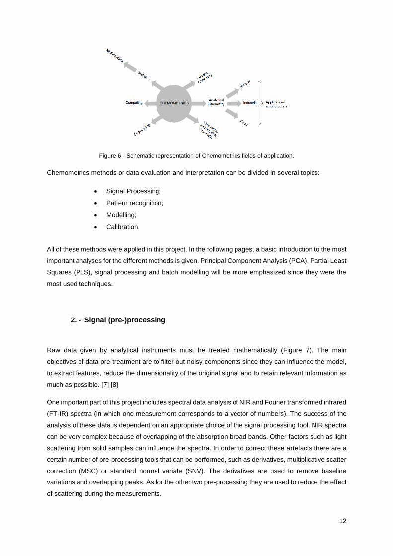
Multivariate data analysis techniques derive from Chemometrics. The word Chemometrics was first
introduced in the 70’s by the Swedish Svante Wold and the American Bruce R. Kowalski. By that time
Chemometrics was strongly correlated to analytical chemistry, being first applied on the food industry.
Since then it has evolved into many other areas, such as organic chemistry and engineering (Figure 6).
[5]
Nowadays the most known definition of Chemometrics is: a chemical science that uses statistical and
mathematical models to design or select optimal measurement procedures and experiments, and
provide maximum chemical information of the studied process with the analysis of collected data. [5] [6]
12
Figure 6 - Schematic representation of Chemometrics fields of application.
Chemometrics methods or data evaluation and interpretation can be divided in several topics:
Signal Processing;
Pattern recognition;
Modelling;
Calibration.
All of these methods were applied in this project. In the following pages, a basic introduction to the most
important analyses for the different methods is given. Principal Component Analysis (PCA), Partial Least
Squares (PLS), signal processing and batch modelling will be more emphasized since they were the
most used techniques.
2. - Signal (pre-)processing
Raw data given by analytical instruments must be treated mathematically (Figure 7). The main
objectives of data pre-treatment are to filter out noisy components since they can influence the model,
to extract features, reduce the dimensionality of the original signal and to retain relevant information as
much as possible. [7] [8]
One important part of this project includes spectral data analysis of NIR and Fourier transformed infrared
(FT-IR) spectra (in which one measurement corresponds to a vector of numbers). The success of the
analysis of these data is dependent on an appropriate choice of the signal processing tool. NIR spectra
can be very complex because of overlapping of the absorption broad bands. Other factors such as light
scattering from solid samples can influence the spectra. In order to correct these artefacts there are a
certain number of pre-processing tools that can be performed, such as derivatives, multiplicative scatter
correction (MSC) or standard normal variate (SNV). The derivatives are used to remove baseline
variations and overlapping peaks. As for the other two pre-processing they are used to reduce the effect
of scattering during the measurements.
13
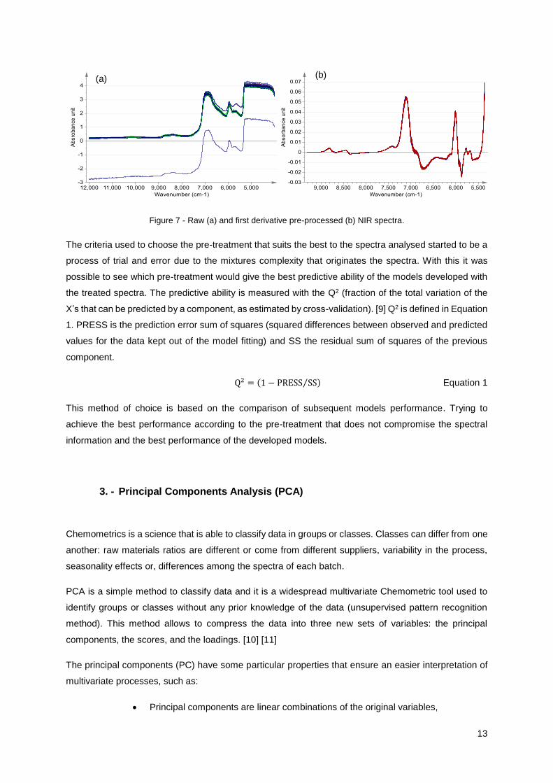
Figure 7 - Raw (a) and first derivative pre-processed (b) NIR spectra.
The criteria used to choose the pre-treatment that suits the best to the spectra analysed started to be a
process of trial and error due to the mixtures complexity that originates the spectra. With this it was
possible to see which pre-treatment would give the best predictive ability of the models developed with
the treated spectra. The predictive ability is measured with the Q2 (fraction of the total variation of the
X’s that can be predicted by a component, as estimated by cross-validation). [9] Q2 is defined in Equation
1. PRESS is the prediction error sum of squares (squared differences between observed and predicted
values for the data kept out of the model fitting) and SS the residual sum of squares of the previous
component.
Q2 = (1 − PRESS SS⁄ ) Equation 1
This method of choice is based on the comparison of subsequent models performance. Trying to
achieve the best performance according to the pre-treatment that does not compromise the spectral
information and the best performance of the developed models.
3. - Principal Components Analysis (PCA)
Chemometrics is a science that is able to classify data in groups or classes. Classes can differ from one
another: raw materials ratios are different or come from different suppliers, variability in the process,
seasonality effects or, differences among the spectra of each batch.
PCA is a simple method to classify data and it is a widespread multivariate Chemometric tool used to
identify groups or classes without any prior knowledge of the data (unsupervised pattern recognition
method). This method allows to compress the data into three new sets of variables: the principal
components, the scores, and the loadings. [10] [11]
The principal components (PC) have some particular properties that ensure an easier interpretation of
multivariate processes, such as:
Principal components are linear combinations of the original variables,
(b) (a)
14
The different principal components are not correlated with each other (orthogonal),
The first principal component describes the greatest source of variation within the
original variables,
The remaining principal components that are relevant take into account the
remaining variability.
The choice of how many PC are relevant is sometimes subjective. It will be the result of balancing
between trying to explain the most variability of a certain data and/or at the same time avoiding
unnecessary information (noise). In order to help in the decision of how many PC are needed to explain
the data, there are some statistical tools such as eigenvalue-one criterion or cross-validation.
Two other sets of variables, the scores, and the loadings contain valuable information for pattern
recognition. The scores measure how samples relate to each other. The pattern recognition is possible
to visualise through a plot of the first PC scores versus the second PC scores (since these two normally
explain a significant amount of the variability present in the dataset). On the other hand, the loadings
measure how the variables relate to each other and which are the most significant variables for the
position of a certain sample in the scores plot.
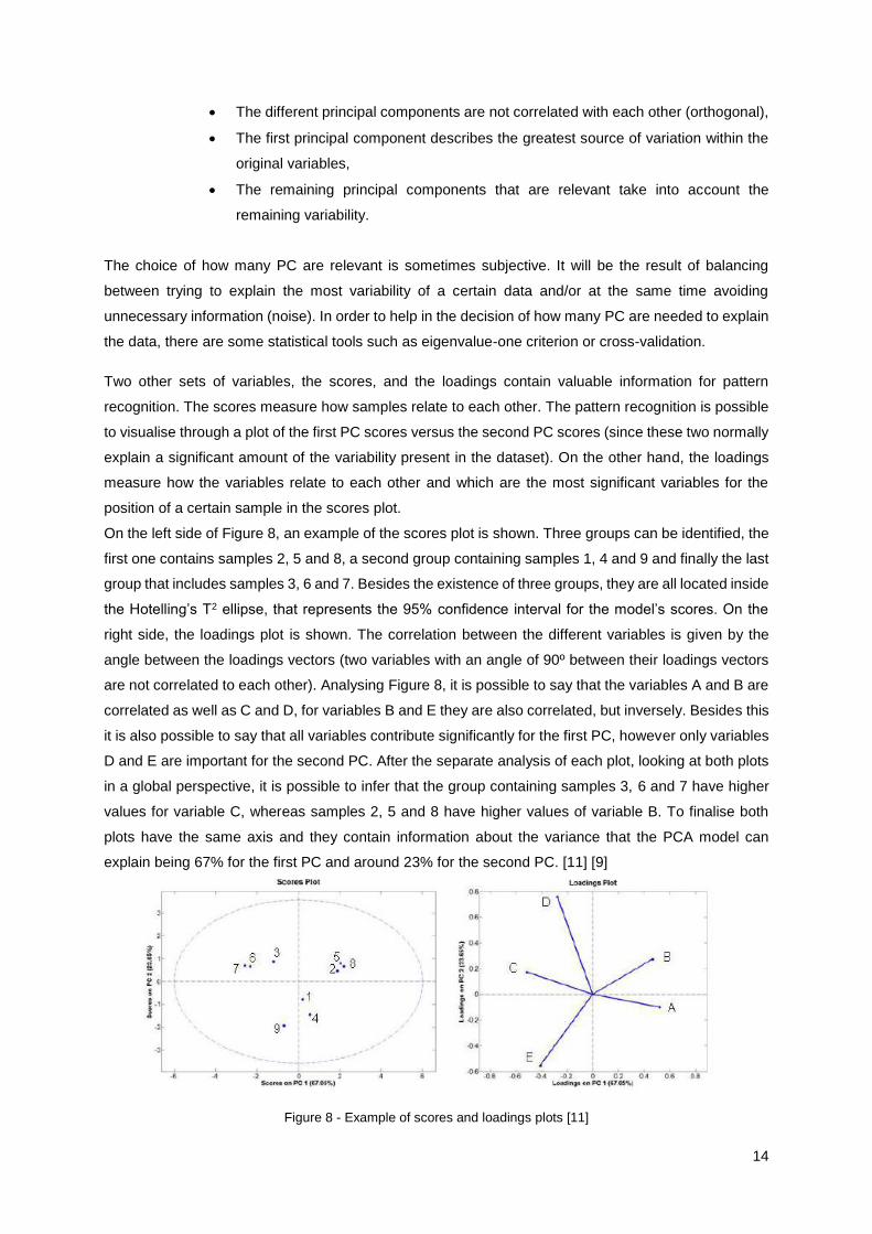
On the left side of Figure 8, an example of the scores plot is shown. Three groups can be identified, the
first one contains samples 2, 5 and 8, a second group containing samples 1, 4 and 9 and finally the last
group that includes samples 3, 6 and 7. Besides the existence of three groups, they are all located inside
the Hotelling’s T2 ellipse, that represents the 95% confidence interval for the model’s scores. On the
right side, the loadings plot is shown. The correlation between the different variables is given by the
angle between the loadings vectors (two variables with an angle of 90º between their loadings vectors
are not correlated to each other). Analysing Figure 8, it is possible to say that the variables A and B are
correlated as well as C and D, for variables B and E they are also correlated, but inversely. Besides this
it is also possible to say that all variables contribute significantly for the first PC, however only variables
D and E are important for the second PC. After the separate analysis of each plot, looking at both plots
in a global perspective, it is possible to infer that the group containing samples 3, 6 and 7 have higher
values for variable C, whereas samples 2, 5 and 8 have higher values of variable B. To finalise both
plots have the same axis and they contain information about the variance that the PCA model can
explain being 67% for the first PC and around 23% for the second PC. [11] [9]
Figure 8 - Example of scores and loadings plots [11]
15
4. - Partial Least Squares (PLS)
Through pattern recognition, multivariate calibration is another application of Chemometrics. In it,
investigation of correlations between a set of measurements that are cheaper and/or easier to acquire
than other measurements are made. After the discovery of these relationships (calibration equations)
the cheapest and easiest measurements (the NIR spectra) can replace the ones that are expensive
(e.g. lab analyses), saving money and time. There are two different sets of variables for PLS methods:
X variables which are independent variables and the other set, Y, which corresponds to dependent
variables. Partial least squares regression (PLS) it is of particular interest because it can analyse
strongly collinear, noisy or incomplete (both in X and Y sets) data. [12] This method condenses the X
information into a new set of variables, the latent variables (LV) in such a way that the covariance
between X and Y is maximised. These latent variables have the same properties as the PC, mentioned
above, for the PCA method. This method was used to predict physical and chemical properties
considering the NIR spectra collected for each batch.
5. - Batch Modelling
In the chemical, pharmaceutical and biotechnological industries, batch-wise processes are very
common. The development and application of batch statistical process control (BSPC) methods is highly
important.
As opposed to a continuous process, a batch process has a finite duration. Generally, the datasets
generated during a process with many variables and observations are time dependent/related. BSPC
analysis allows to determine which variables influence the quality of the final product, how those
variables are correlated to each other and also to distinguish the common batches from the deviating
ones. BSPC will not be a useful tool if the variables monitored during the batches are not sensitive to
variations.
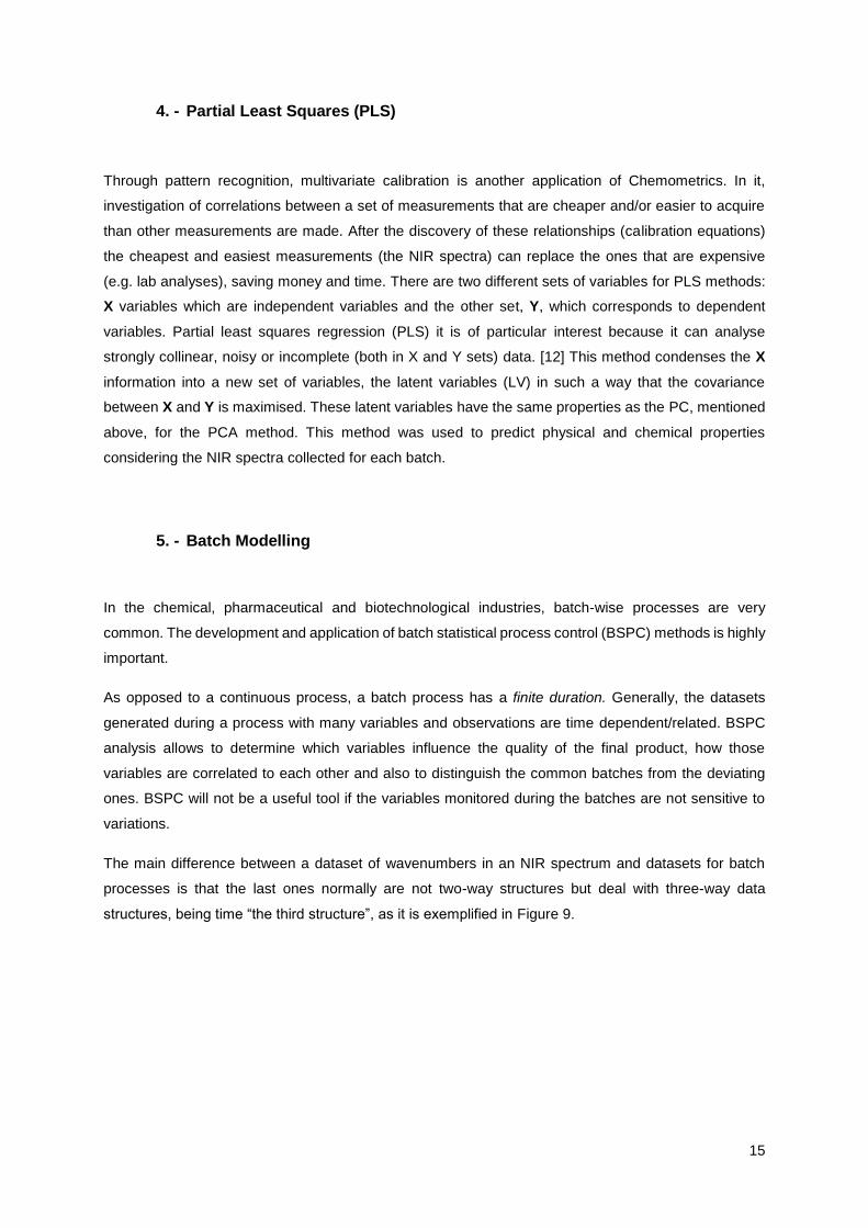
The main difference between a dataset of wavenumbers in an NIR spectrum and datasets for batch
processes is that the last ones normally are not two-way structures but deal with three-way data
structures, being time “the third structure”, as it is exemplified in Figure 9.
16
Figure 9 - Three-way table of batch process data.
The time dependency of the batches can sometimes be challenging since not all batches have the same
duration requiring their alignment. In batch modelling, a maturity variable is used as the basis for batch
synchronisation instead of real time. This maturity variable expresses the degree of batch completion.
Two different levels of batch monitoring are performed: the observation and the batch level.
Observation level monitoring is mainly interesting to (1) evaluate individual observations (such as time
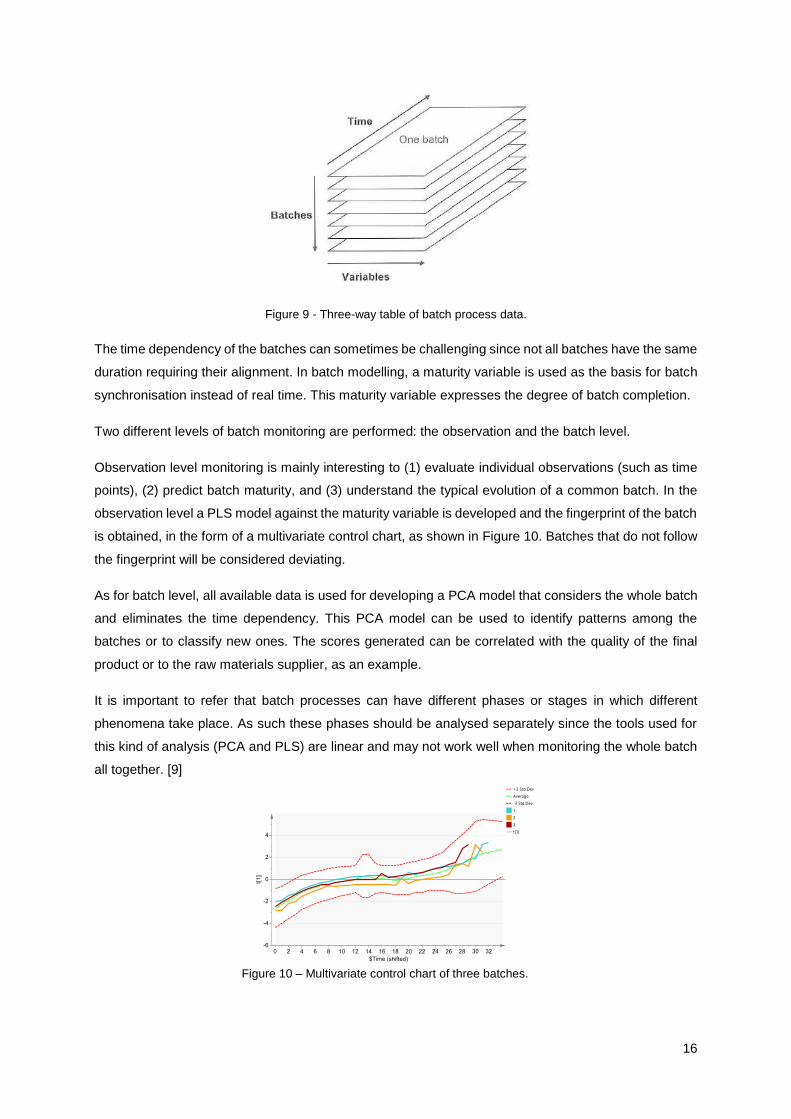
points), (2) predict batch maturity, and (3) understand the typical evolution of a common batch. In the
observation level a PLS model against the maturity variable is developed and the fingerprint of the batch
is obtained, in the form of a multivariate control chart, as shown in Figure 10. Batches that do not follow
the fingerprint will be considered deviating.
As for batch level, all available data is used for developing a PCA model that considers the whole batch
and eliminates the time dependency. This PCA model can be used to identify patterns among the
batches or to classify new ones. The scores generated can be correlated with the quality of the final
product or to the raw materials supplier, as an example.
It is important to refer that batch processes can have different phases or stages in which different
phenomena take place. As such these phases should be analysed separately since the tools used for
this kind of analysis (PCA and PLS) are linear and may not work well when monitoring the whole batch
all together. [9]
Figure 10 – Multivariate control chart of three batches.
17
Chapter V. - Vibrational spectroscopies
The demand for product quality improvement has been increasing in many industries like (petro)
chemical, polymer, pharmaceutical, food, in the last few years. This increase led to a gradual substitution
of classic analytical techniques (Gel Permeation Chromatography (GPC), High-Performance Liquid
Chromatography (HPLC), Nuclear Molecular Resonance (NMR)) and non-specific chemical analyses
(pH, viscosity, temperature or pressure) for more specific, environmentally compatible and faster
analytical tools. These analytical tools are the different methods of vibrational spectroscopies (FT-IR,
NIR and Raman) that allow for non-destructive and fast measurements almost without any need of
sample preparation. [13] This kind of analyses can be executed off-line, at-line or even in-line,
contributing all for quality monitoring of the raw materials and also for the final products. During this
project, NIR and FT-IR spectroscopies were used, FT-IR for raw materials quality check and NIR for the
finished resin. The FT-IR device used at Trespa is a Spectrum Two IR Spectrometer (Perkin Elmer,
Massachusetts, USA), see Figure 11 (a), and for NIR an MPA FT-NIR spectrometer (Brüker,
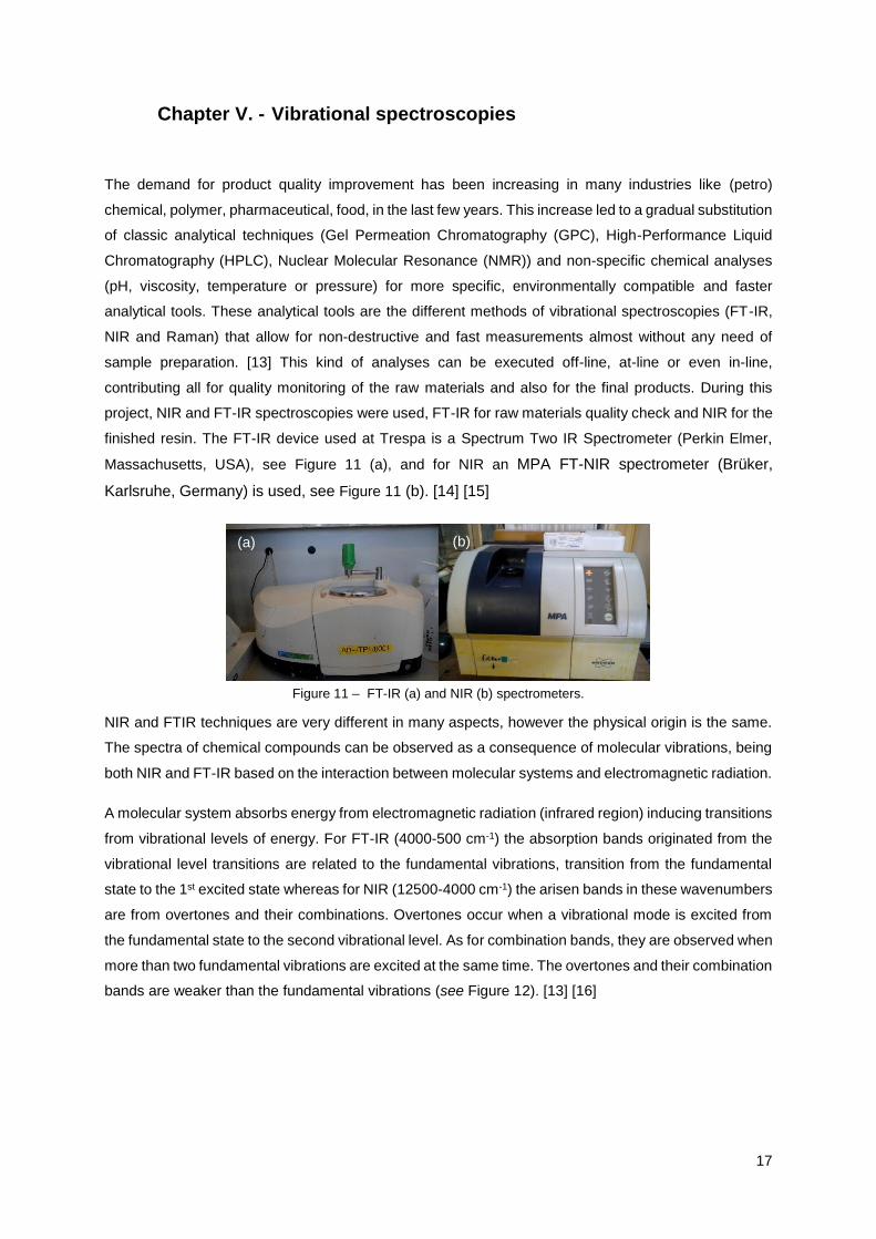
Karlsruhe, Germany) is used, see Figure 11 (b). [14] [15]
NIR and FTIR techniques are very different in many aspects, however the physical origin is the same.
The spectra of chemical compounds can be observed as a consequence of molecular vibrations, being
both NIR and FT-IR based on the interaction between molecular systems and electromagnetic radiation.
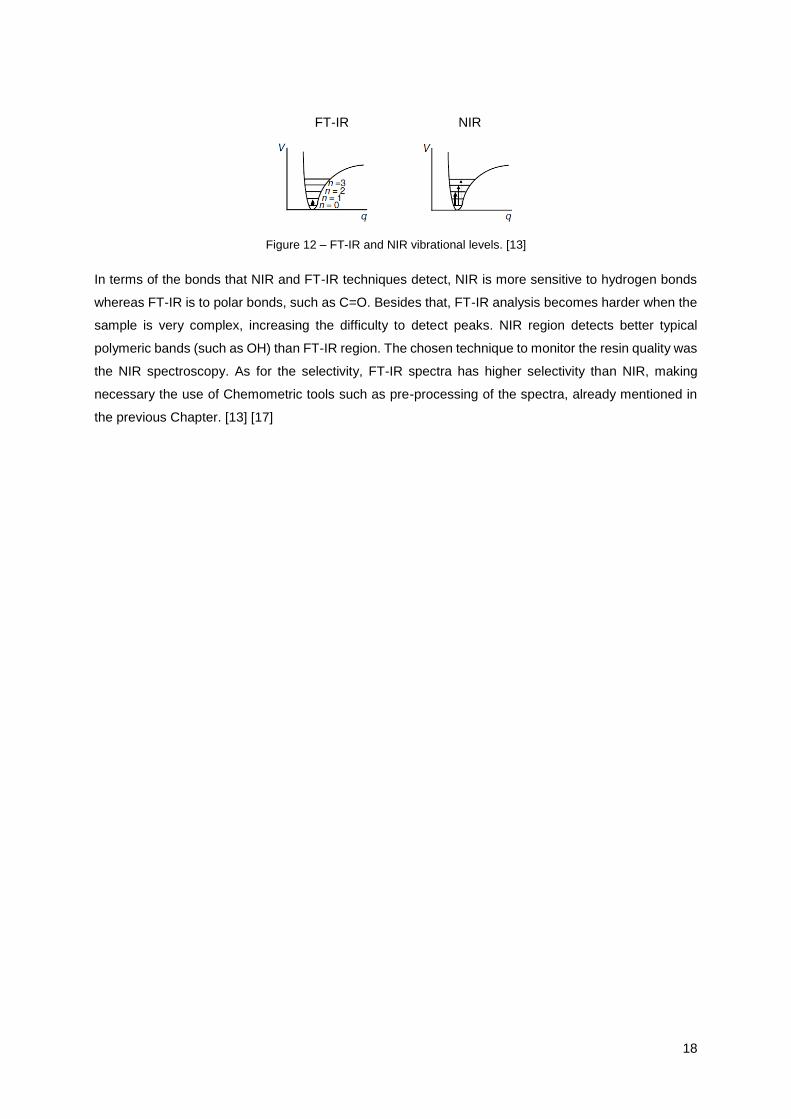
A molecular system absorbs energy from electromagnetic radiation (infrared region) inducing transitions
from vibrational levels of energy. For FT-IR (4000-500 cm-1) the absorption bands originated from the
vibrational level transitions are related to the fundamental vibrations, transition from the fundamental
state to the 1st excited state whereas for NIR (12500-4000 cm-1) the arisen bands in these wavenumbers
are from overtones and their combinations. Overtones occur when a vibrational mode is excited from
the fundamental state to the second vibrational level. As for combination bands, they are observed when
more than two fundamental vibrations are excited at the same time. The overtones and their combination
bands are weaker than the fundamental vibrations (see Figure 12). [13] [16]
Figure 11 – FT-IR (a) and NIR (b) spectrometers.
(b) (a)
18
Figure 12 – FT-IR and NIR vibrational levels. [13]
In terms of the bonds that NIR and FT-IR techniques detect, NIR is more sensitive to hydrogen bonds
whereas FT-IR is to polar bonds, such as C=O. Besides that, FT-IR analysis becomes harder when the
sample is very complex, increasing the difficulty to detect peaks. NIR region detects better typical
polymeric bands (such as OH) than FT-IR region. The chosen technique to monitor the resin quality was
the NIR spectroscopy. As for the selectivity, FT-IR spectra has higher selectivity than NIR, making
necessary the use of Chemometric tools such as pre-processing of the spectra, already mentioned in
the previous Chapter. [13] [17]
FT-IR NIR
19
Chapter VI. - Physical and chemical characterisation of resins
The determination of the structure and physical-chemical properties of a resin is revealed with some lab
analyses. For each resin sample, the analyses performed were: viscosity, curing speed time, tolerance
to water, HPLC, GPC, formaldehyde and phenol contents, percentage of solids, and pH. [18]
The resin viscosity was measured in a DV2T Viscometer (Brookfield AMETEK Inc., Middleboro,
MA, USA) at 20ºC and 100 r.p.m. during 1 minute. This physical property gives a direct
indication of the manageability of the resin in production and also the size of the polymer.
For the curing speed of the resin B-time measurement was performed using a heated plate (Gel
instrument AG, Oberuzwil, Switzerland) at 120ºC. Ca. 1 mL of the resin was added to the heated
plate and stirred until the resin was totally cured. If a resin has higher curing speed time it
probably means that the curing of the resin during the reaction was shorter, being the polymer
smaller. The curing process also gives important information for the pressing process. A longer
pressing cycle (high curing) leads to a structural deterioration of the panel due to high shrinking.
The water tolerance measurement allows to see if the resin can be diluted with water and also
the amount of water that a resin can carry before it starts precipitating. This measurement is
done with 5-10 g of resin in which water is added until the resin becomes turbid. After every
addition of water stirring is required to make sure that the mixture is homogeneous.
The percentage of solids is measured by drying the resin for 3 hours in an oven type FED 53
(Binder, Tuttlingen, Germany) at 135ºC. This analysis gives an indication of the amount of solid
impurities coming from raw materials.
The pH determination is performed in a HI2211 equipment (Hanna Instruments, Limena, Italy),
that features automatic calibration to 1 or 2 points. All the readings are compensated
automatically for temperature variations by the supplied thermistor probe. The pH allows to
measure the amount of basic catalyst that is still present in the resin at the end of the batch.
To quantify which components are present in the resin and the molecular weight of the polymer, HPLC
and GPC were used. Those techniques were performed in an Alliance 2690/2690D Separations Module
Upgrade (Waters Corp., Milford, MA, USA).
HPLC was performed to quantify the phenol content. The amount of formaldehyde is measured
by titration. For resins with fire retardant additives, the amount of formaldehyde has to be
performed by HPLC. GPC measures the molecular weight and polydispersity of the resin. All
these measurements are of extreme importance since they give a direct indication of the
performance of the process. The quality of the resin is measured with GPC and HPLC, e.g.
higher phenol content indicates a lower molecular weight thus less condensation. The same
conclusion can be applied for the formaldehyde content. Both GPC and HPLC were performed
by a technician from Trespa.

20
The titration to determine the formaldehyde content is performed according to the norm DIN EN
ISO 11402 in an 848 Titrino Plus (Metrohm, Herisau, Switzerland). [19]
21
Part B. - Results and Discussion
Chapter I. - Study of raw materials variability
The analysis of the variability of raw materials precedes the study of resins. As mentioned before, every
supply truck that comes to Trespa with all the raw materials is inspected. A sample of each truck is
analysed through spectroscopy (FT-IR) and the collected spectra are saved in a database.
These spectra are also used to conclude if the raw material, inside the truck, complies with the reference
spectrum, using a correlation factor. The reference spectrum is known to correspond to a raw material
that complies with what is agreed to be supplied. The whole spectrum is taken into account. As for the
correlation factor, it is used to find the similarities between the reference and the analysed spectrum
giving a relative similarity factor. If the sample spectrum of the truck has a similarity factor higher or
equal to the one established for the raw material analysed, the truck can be unloaded to the
corresponding storage tank.
In this thesis, multivariate data analysis was performed to the collected spectra to investigate variability
of the raw materials. Some of the raw materials are supplied by more than one supplier. Differences
among the suppliers were also investigated, as the suppliers can provide different raw materials quality.
Nevertheless, both suppliers can comply to the specifications agreed with Trespa. All these variations
can have further impact on the production process and on resin quality, which will be investigated in the
next Chapters.
To produce a resin, formaldehyde and phenol are the main raw materials, yet for, some of the studied
resins, a diluent and other special additives are also needed. For each of those raw materials,
exploratory analysis was performed from 2013 until mid-2016. PCA was performed for each of the
spectral datasets. In order to improve the models results, the spectra were pre-processed. The pre-
processing was applied to each of the raw materials. A few spectra were not properly collected, having
been eliminated from the dataset. Some of the spectral zones of the different raw materials datasets
showed noise, which were also excluded. This analysis was performed using the MVDA software
programme SOLO 8.1.1 (Eigenvector Research Inc., Washington, USA).
1. - Phenol
The phenol used to produce the resins is purchased by Trespa in both pure (99% purity) and impure
forms (80% of phenolic compounds). Both of these are widely used as one of the main raw materials
for all the types of resins. It is of extreme importance to analyse the variability and/or quality of this raw
material.
22
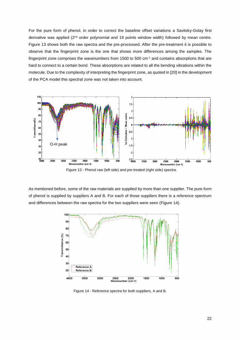
For the pure form of phenol, in order to correct the baseline offset variations a Savitsky-Golay first
derivative was applied (2nd order polynomial and 19 points window width) followed by mean centre.
Figure 13 shows both the raw spectra and the pre-processed. After the pre-treatment it is possible to
observe that the fingerprint zone is the one that shows more differences among the samples. The
fingerprint zone comprises the wavenumbers from 1500 to 500 cm-1 and contains absorptions that are
hard to connect to a certain bond. These absorptions are related to all the bending vibrations within the
molecule. Due to the complexity of interpreting the fingerprint zone, as quoted in [20] in the development
of the PCA model this spectral zone was not taken into account.
As mentioned before, some of the raw materials are supplied by more than one supplier. The pure form
of phenol is supplied by suppliers A and B. For each of those suppliers there is a reference spectrum
and differences between the raw spectra for the two suppliers were seen (Figure 14).
Figure 14 - Reference spectra for both suppliers, A and B.
Figure 13 - Phenol raw (left side) and pre-treated (right side) spectra.
O-H peak
23
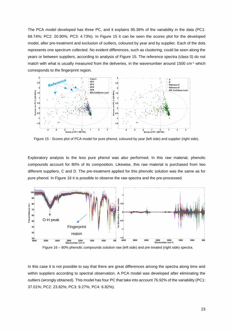
The PCA model developed has three PC, and it explains 95.36% of the variability in the data (PC1:
69.74%; PC2: 20.90%; PC3: 4.73%). In Figure 15 it can be seen the scores plot for the developed
model, after pre-treatment and exclusion of outliers, coloured by year and by supplier. Each of the dots
represents one spectrum collected. No evident differences, such as clustering, could be seen along the
years or between suppliers, according to analysis of Figure 15. The reference spectra (class 0) do not
match with what is usually measured from the deliveries, in the wavenumber around 1500 cm-1 which
corresponds to the fingerprint region.
Exploratory analysis to the less pure phenol was also performed. In this raw material, phenolic
compounds account for 80% of its composition. Likewise, this raw material is purchased from two
different suppliers, C and D. The pre-treatment applied for this phenolic solution was the same as for
pure phenol. In Figure 16 it is possible to observe the raw spectra and the pre-processed.
In this case it is not possible to say that there are great differences among the spectra along time and
within suppliers according to spectral observation. A PCA model was developed after eliminating the
outliers (wrongly obtained). This model has four PC that take into account 76.92% of the variability (PC1:
37.01%; PC2: 23.82%; PC3: 9.27%; PC4: 6.82%).
Figure 16 – 80% phenolic compounds solution raw (left side) and pre-treated (right side) spectra.
Figure 15 - Scores plot of PCA model for pure phenol, coloured by year (left side) and supplier (right side).
O-H peak
Fingerprint
region
24
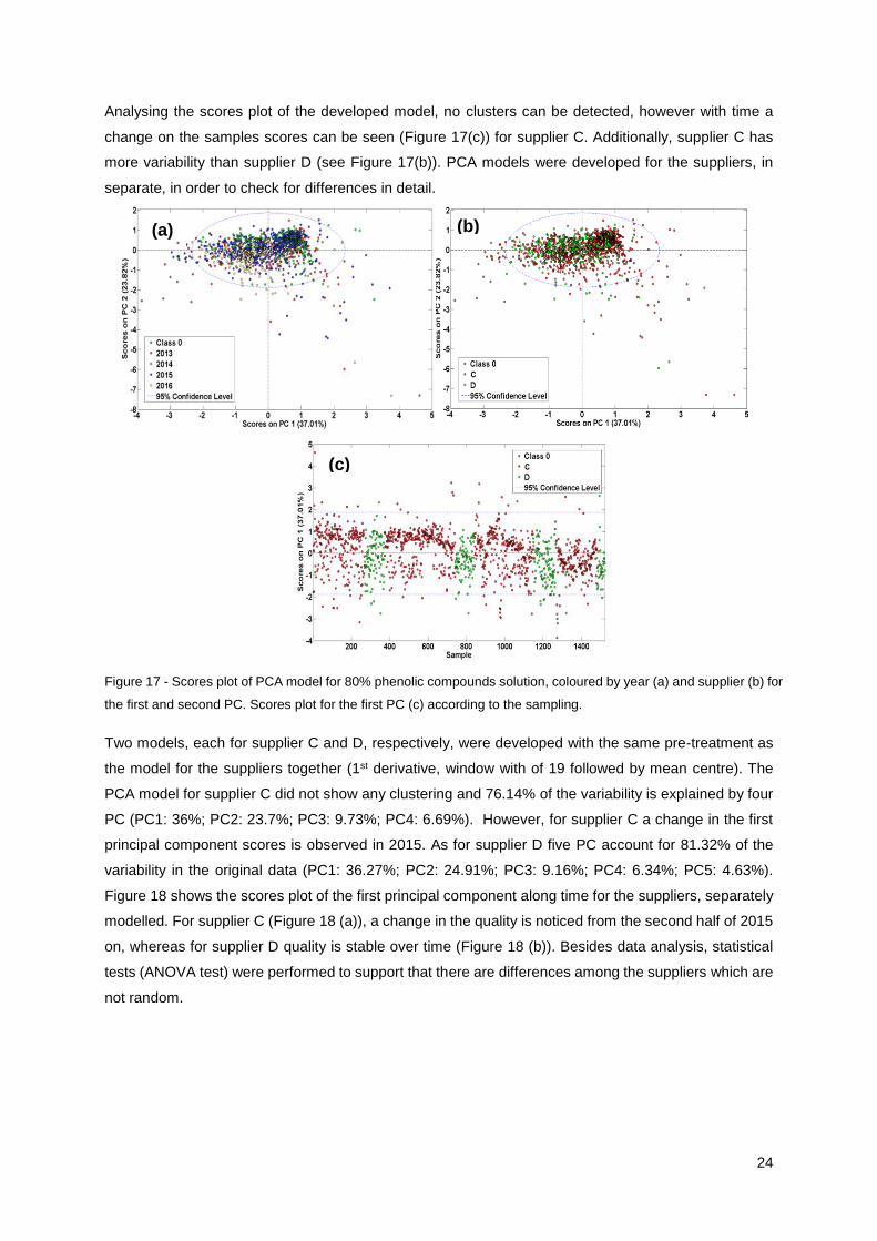
Analysing the scores plot of the developed model, no clusters can be detected, however with time a
change on the samples scores can be seen (Figure 17(c)) for supplier C. Additionally, supplier C has
more variability than supplier D (see Figure 17(b)). PCA models were developed for the suppliers, in
separate, in order to check for differences in detail.
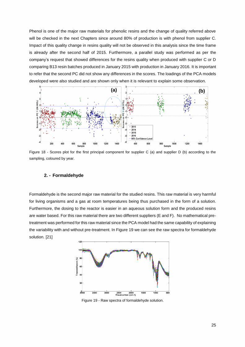
Two models, each for supplier C and D, respectively, were developed with the same pre-treatment as
the model for the suppliers together (1st derivative, window with of 19 followed by mean centre). The
PCA model for supplier C did not show any clustering and 76.14% of the variability is explained by four
PC (PC1: 36%; PC2: 23.7%; PC3: 9.73%; PC4: 6.69%). However, for supplier C a change in the first
principal component scores is observed in 2015. As for supplier D five PC account for 81.32% of the
variability in the original data (PC1: 36.27%; PC2: 24.91%; PC3: 9.16%; PC4: 6.34%; PC5: 4.63%).
Figure 18 shows the scores plot of the first principal component along time for the suppliers, separately
modelled. For supplier C (Figure 18 (a)), a change in the quality is noticed from the second half of 2015
on, whereas for supplier D quality is stable over time (Figure 18 (b)). Besides data analysis, statistical
tests (ANOVA test) were performed to support that there are differences among the suppliers which are
not random.
(a) (b)
(c)
Figure 17 - Scores plot of PCA model for 80% phenolic compounds solution, coloured by year (a) and supplier (b) for
the first and second PC. Scores plot for the first PC (c) according to the sampling.
25
Phenol is one of the major raw materials for phenolic resins and the change of quality referred above
will be checked in the next Chapters since around 80% of production is with phenol from supplier C.
Impact of this quality change in resins quality will not be observed in this analysis since the time frame
is already after the second half of 2015. Furthermore, a parallel study was performed as per the
company’s request that showed differences for the resins quality when produced with supplier C or D
comparing B13 resin batches produced in January 2015 with production in January 2016. It is important
to refer that the second PC did not show any differences in the scores. The loadings of the PCA models
developed were also studied and are shown only when it is relevant to explain some observation.
2. - Formaldehyde
Formaldehyde is the second major raw material for the studied resins. This raw material is very harmful
for living organisms and a gas at room temperatures being thus purchased in the form of a solution.
Furthermore, the dosing to the reactor is easier in an aqueous solution form and the produced resins
are water based. For this raw material there are two different suppliers (E and F). No mathematical pre-
treatment was performed for this raw material since the PCA model had the same capability of explaining
the variability with and without pre-treatment. In Figure 19 we can see the raw spectra for formaldehyde
solution. [21]
Figure 19 - Raw spectra of formaldehyde solution.
Figure 18 - Scores plot for the first principal component for supplier C (a) and supplier D (b) according to the
sampling, coloured by year.
(a) (b)
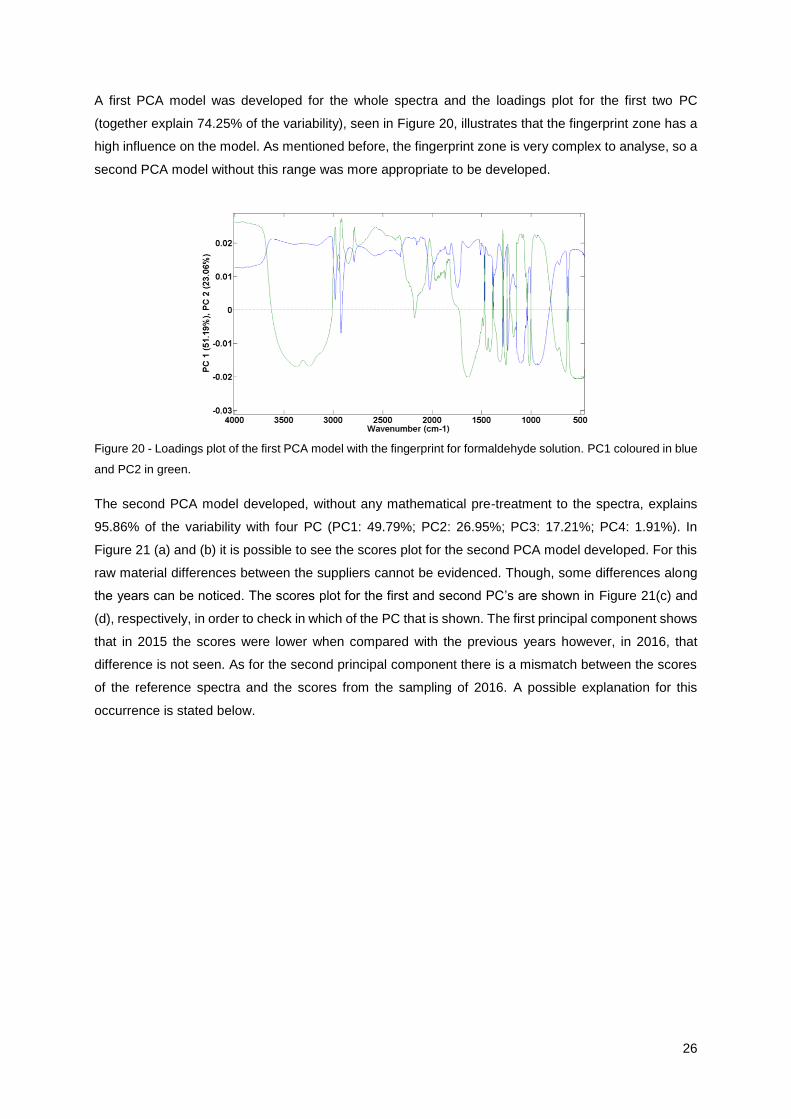
26
A first PCA model was developed for the whole spectra and the loadings plot for the first two PC
(together explain 74.25% of the variability), seen in Figure 20, illustrates that the fingerprint zone has a
high influence on the model. As mentioned before, the fingerprint zone is very complex to analyse, so a
second PCA model without this range was more appropriate to be developed.
Figure 20 - Loadings plot of the first PCA model with the fingerprint for formaldehyde solution. PC1 coloured in blue
and PC2 in green.
The second PCA model developed, without any mathematical pre-treatment to the spectra, explains
95.86% of the variability with four PC (PC1: 49.79%; PC2: 26.95%; PC3: 17.21%; PC4: 1.91%). In
Figure 21 (a) and (b) it is possible to see the scores plot for the second PCA model developed. For this
raw material differences between the suppliers cannot be evidenced. Though, some differences along
the years can be noticed. The scores plot for the first and second PC’s are shown in Figure 21(c) and
(d), respectively, in order to check in which of the PC that is shown. The first principal component shows
that in 2015 the scores were lower when compared with the previous years however, in 2016, that
difference is not seen. As for the second principal component there is a mismatch between the scores
of the reference spectra and the scores from the sampling of 2016. A possible explanation for this
occurrence is stated below.
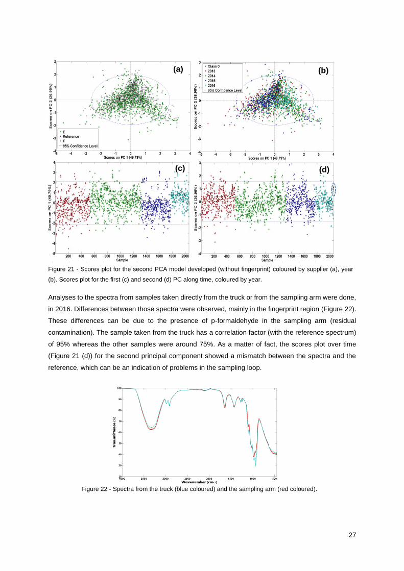
27
SDGDFH
Analyses to the spectra from samples taken directly from the truck or from the sampling arm were done,
in 2016. Differences between those spectra were observed, mainly in the fingerprint region (Figure 22).
These differences can be due to the presence of p-formaldehyde in the sampling arm (residual
contamination). The sample taken from the truck has a correlation factor (with the reference spectrum)
of 95% whereas the other samples were around 75%. As a matter of fact, the scores plot over time
(Figure 21 (d)) for the second principal component showed a mismatch between the spectra and the
reference, which can be an indication of problems in the sampling loop.
Figure 22 - Spectra from the truck (blue coloured) and the sampling arm (red coloured).
(a) (b)
(c) (d)
Figure 21 - Scores plot for the second PCA model developed (without fingerprint) coloured by supplier (a), year
(b). Scores plot for the first (c) and second (d) PC along time, coloured by year.
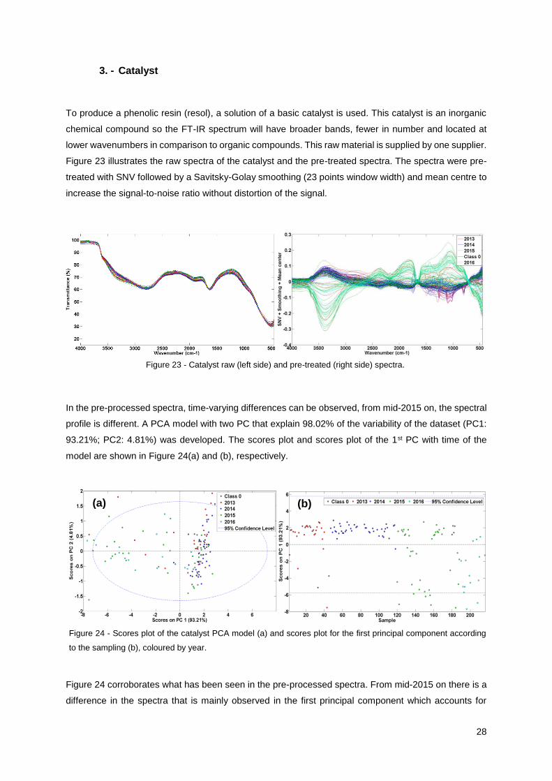
28
3. - Catalyst
To produce a phenolic resin (resol), a solution of a basic catalyst is used. This catalyst is an inorganic
chemical compound so the FT-IR spectrum will have broader bands, fewer in number and located at
lower wavenumbers in comparison to organic compounds. This raw material is supplied by one supplier.
Figure 23 illustrates the raw spectra of the catalyst and the pre-treated spectra. The spectra were pre-
treated with SNV followed by a Savitsky-Golay smoothing (23 points window width) and mean centre to
increase the signal-to-noise ratio without distortion of the signal.
In the pre-processed spectra, time-varying differences can be observed, from mid-2015 on, the spectral
profile is different. A PCA model with two PC that explain 98.02% of the variability of the dataset (PC1:
93.21%; PC2: 4.81%) was developed. The scores plot and scores plot of the 1st PC with time of the
model are shown in Figure 24(a) and (b), respectively.
Figure 24 corroborates what has been seen in the pre-processed spectra. From mid-2015 on there is a
difference in the spectra that is mainly observed in the first principal component which accounts for
Figure 24 - Scores plot of the catalyst PCA model (a) and scores plot for the first principal component according
to the sampling (b), coloured by year.
(a) (b)
Figure 23 - Catalyst raw (left side) and pre-treated (right side) spectra.
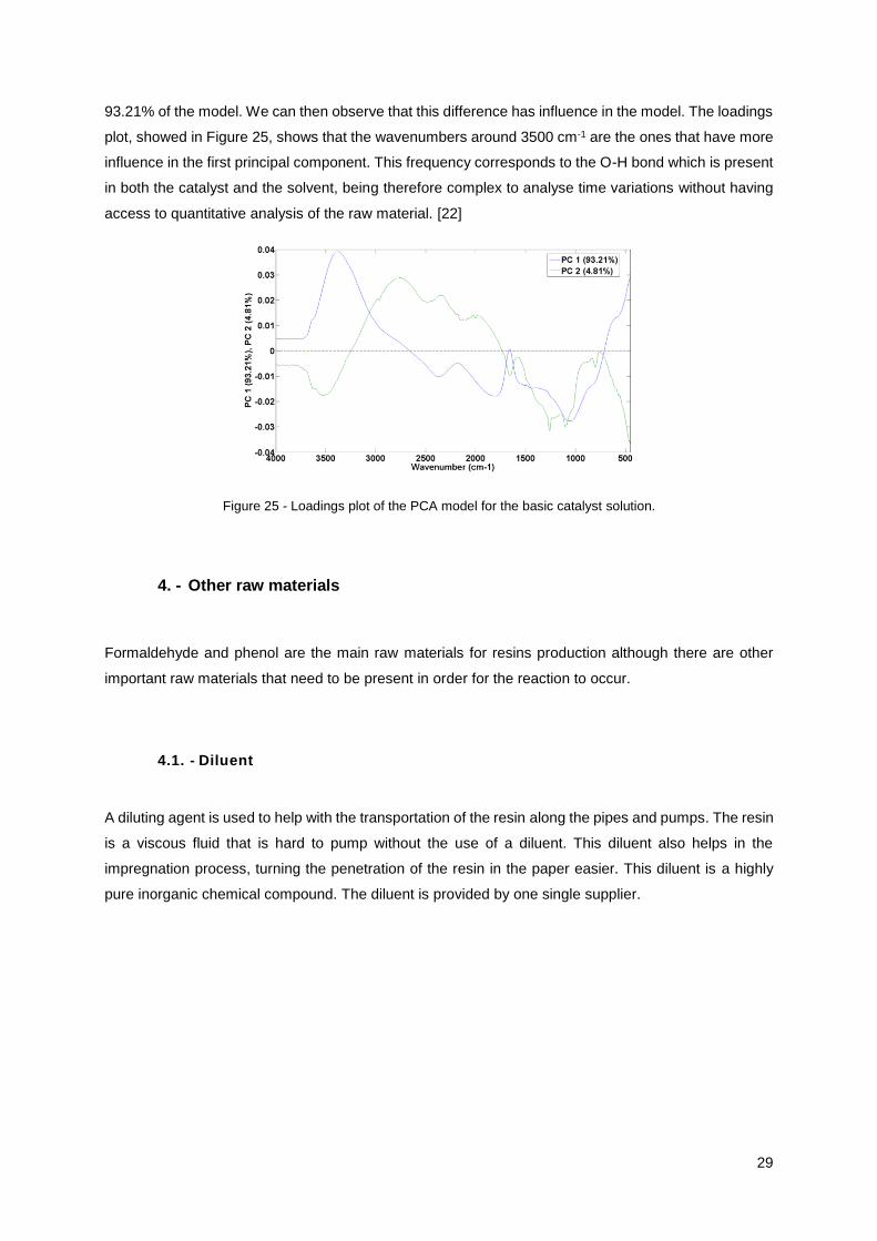
29
93.21% of the model. We can then observe that this difference has influence in the model. The loadings
plot, showed in Figure 25, shows that the wavenumbers around 3500 cm-1 are the ones that have more
influence in the first principal component. This frequency corresponds to the O-H bond which is present
in both the catalyst and the solvent, being therefore complex to analyse time variations without having
access to quantitative analysis of the raw material. [22]
Figure 25 - Loadings plot of the PCA model for the basic catalyst solution.
4. - Other raw materials
Formaldehyde and phenol are the main raw materials for resins production although there are other
important raw materials that need to be present in order for the reaction to occur.
4.1. - Diluent
A diluting agent is used to help with the transportation of the resin along the pipes and pumps. The resin
is a viscous fluid that is hard to pump without the use of a diluent. This diluent also helps in the
impregnation process, turning the penetration of the resin in the paper easier. This diluent is a highly
pure inorganic chemical compound. The diluent is provided by one single supplier.
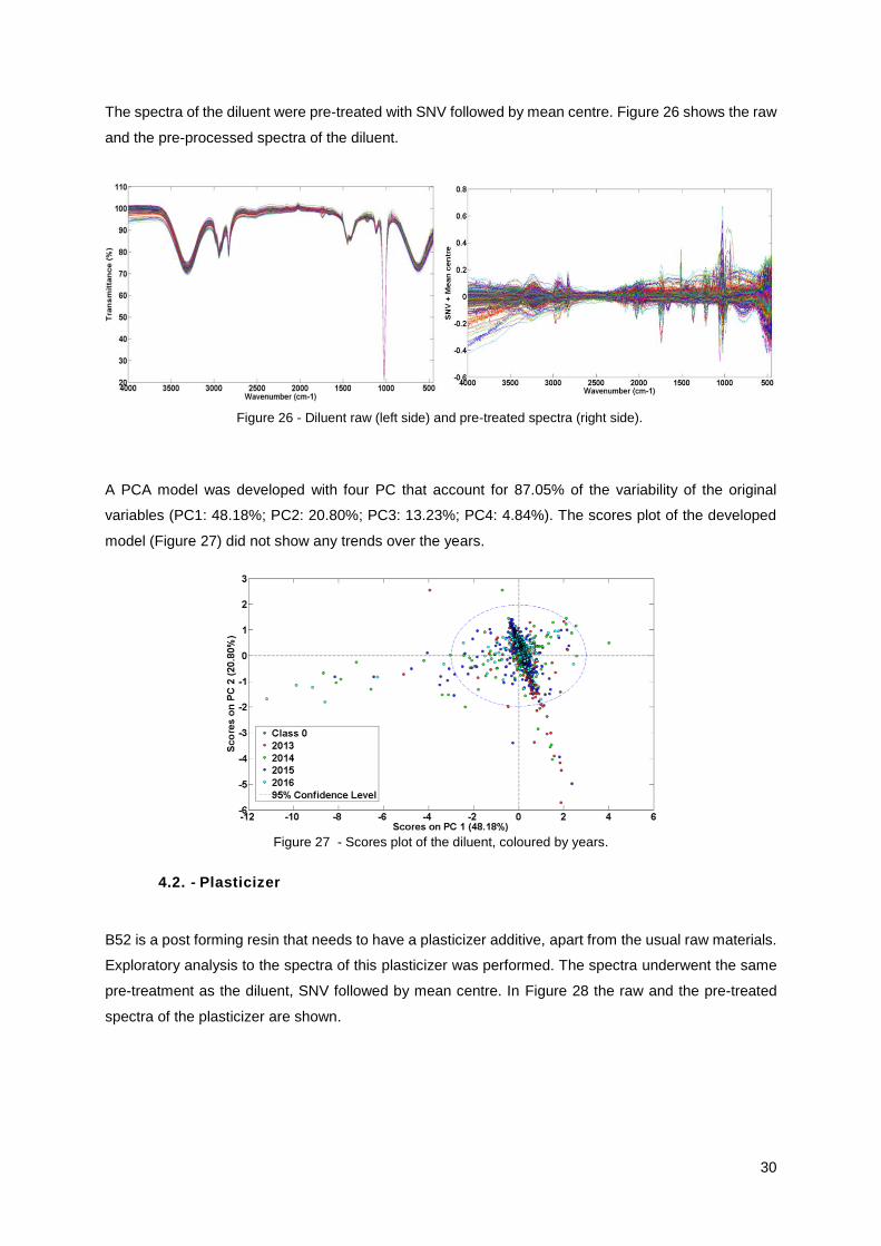
30
The spectra of the diluent were pre-treated with SNV followed by mean centre. Figure 26 shows the raw
and the pre-processed spectra of the diluent.
A PCA model was developed with four PC that account for 87.05% of the variability of the original
variables (PC1: 48.18%; PC2: 20.80%; PC3: 13.23%; PC4: 4.84%). The scores plot of the developed
model (Figure 27) did not show any trends over the years.
Figure 27 - Scores plot of the diluent, coloured by years.
4.2. - Plasticizer
B52 is a post forming resin that needs to have a plasticizer additive, apart from the usual raw materials.
Exploratory analysis to the spectra of this plasticizer was performed. The spectra underwent the same
pre-treatment as the diluent, SNV followed by mean centre. In Figure 28 the raw and the pre-treated
spectra of the plasticizer are shown.
Figure 26 - Diluent raw (left side) and pre-treated spectra (right side).
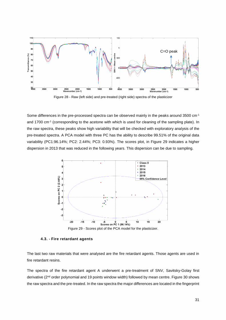
31
Some differences in the pre-processed spectra can be observed mainly in the peaks around 3500 cm-1
and 1700 cm-1 (corresponding to the acetone with which is used for cleaning of the sampling plate). In
the raw spectra, these peaks show high variability that will be checked with exploratory analysis of the
pre-treated spectra. A PCA model with three PC has the ability to describe 99.51% of the original data
variability (PC1:96.14%; PC2: 2.44%; PC3: 0.93%). The scores plot, in Figure 29 indicates a higher
dispersion in 2013 that was reduced in the following years. This dispersion can be due to sampling.
Figure 29 - Scores plot of the PCA model for the plasticizer.
4.3. - Fire retardant agents
The last two raw materials that were analysed are the fire retardant agents. Those agents are used in
fire retardant resins.
The spectra of the fire retardant agent A underwent a pre-treatment of SNV, Savitsky-Golay first
derivative (2nd order polynomial and 19 points window width) followed by mean centre. Figure 30 shows
the raw spectra and the pre-treated. In the raw spectra the major differences are located in the fingerprint
Figure 28 - Raw (left side) and pre-treated (right side) spectra of the plasticizer
C=O peak
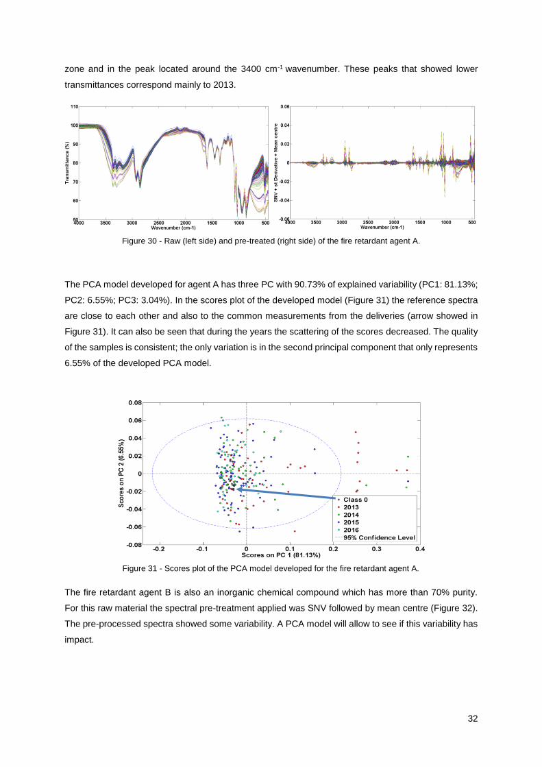
32
zone and in the peak located around the 3400 cm-1 wavenumber. These peaks that showed lower
transmittances correspond mainly to 2013.
The PCA model developed for agent A has three PC with 90.73% of explained variability (PC1: 81.13%;
PC2: 6.55%; PC3: 3.04%). In the scores plot of the developed model (Figure 31) the reference spectra
are close to each other and also to the common measurements from the deliveries (arrow showed in
Figure 31). It can also be seen that during the years the scattering of the scores decreased. The quality
of the samples is consistent; the only variation is in the second principal component that only represents
6.55% of the developed PCA model.
The fire retardant agent B is also an inorganic chemical compound which has more than 70% purity.
For this raw material the spectral pre-treatment applied was SNV followed by mean centre (Figure 32).
The pre-processed spectra showed some variability. A PCA model will allow to see if this variability has
impact.
Figure 30 - Raw (left side) and pre-treated (right side) of the fire retardant agent A.
Figure 31 - Scores plot of the PCA model developed for the fire retardant agent A.
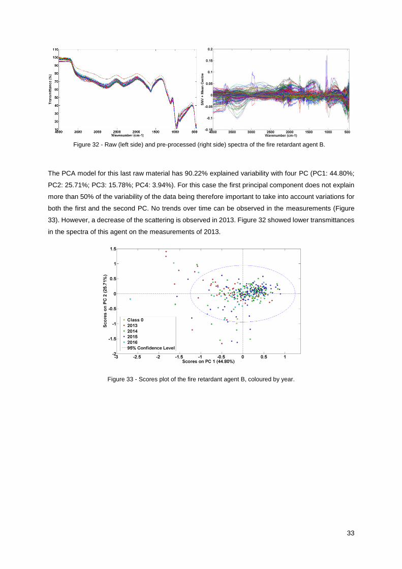
33
The PCA model for this last raw material has 90.22% explained variability with four PC (PC1: 44.80%;
PC2: 25.71%; PC3: 15.78%; PC4: 3.94%). For this case the first principal component does not explain
more than 50% of the variability of the data being therefore important to take into account variations for
both the first and the second PC. No trends over time can be observed in the measurements (Figure
33). However, a decrease of the scattering is observed in 2013. Figure 32 showed lower transmittances
in the spectra of this agent on the measurements of 2013.
Figure 33 - Scores plot of the fire retardant agent B, coloured by year.
Figure 32 - Raw (left side) and pre-processed (right side) spectra of the fire retardant agent B.
34
5. - Conclusions
This Chapter has shown that the FT-IR spectra of the raw materials contains information that can be
extracted with MVDA techniques. With the analysis of the raw materials spectra a great insight into the
differences was achieved.
Significant differences between the suppliers could be identified for the less pure phenol, further
analyses will show the impact of these on the final quality of resins;
Mismatches of the reference spectra and the common measurements could be pointed out: a
review on the references should be done in order to check if it is a sampling problem;
Differences of the spectra along the years were identified. These differences can be related to
problems with the sampling of the trucks or contamination of the sampling arms.
In the next Chapters, it will be checked if the mentioned findings have impact on the resins quality.
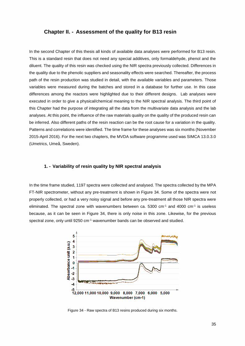
35
Chapter II. - Assessment of the quality for B13 resin
In the second Chapter of this thesis all kinds of available data analyses were performed for B13 resin.
This is a standard resin that does not need any special additives, only formaldehyde, phenol and the
diluent. The quality of this resin was checked using the NIR spectra previously collected. Differences in
the quality due to the phenolic suppliers and seasonality effects were searched. Thereafter, the process
path of the resin production was studied in detail, with the available variables and parameters. Those
variables were measured during the batches and stored in a database for further use. In this case
differences among the reactors were highlighted due to their different designs. Lab analyses were
executed in order to give a physical/chemical meaning to the NIR spectral analysis. The third point of
this Chapter had the purpose of integrating all the data from the multivariate data analysis and the lab
analyses. At this point, the influence of the raw materials quality on the quality of the produced resin can
be inferred. Also different paths of the resin reaction can be the root cause for a variation in the quality.
Patterns and correlations were identified. The time frame for these analyses was six months (November
2015-April 2016). For the next two chapters, the MVDA software programme used was SIMCA 13.0.3.0
(Umetrics, Umeå, Sweden).
1. - Variability of resin quality by NIR spectral analysis
In the time frame studied, 1197 spectra were collected and analysed. The spectra collected by the MPA
FT-NIR spectrometer, without any pre-treatment is shown in Figure 34. Some of the spectra were not
properly collected, or had a very noisy signal and before any pre-treatment all those NIR spectra were
eliminated. The spectral zone with wavenumbers between ca. 5300 cm-1 and 4000 cm-1 is useless
because, as it can be seen in Figure 34, there is only noise in this zone. Likewise, for the previous
spectral zone, only until 9250 cm-1 wavenumber bands can be observed and studied.
Figure 34 - Raw spectra of B13 resins produced during six months.
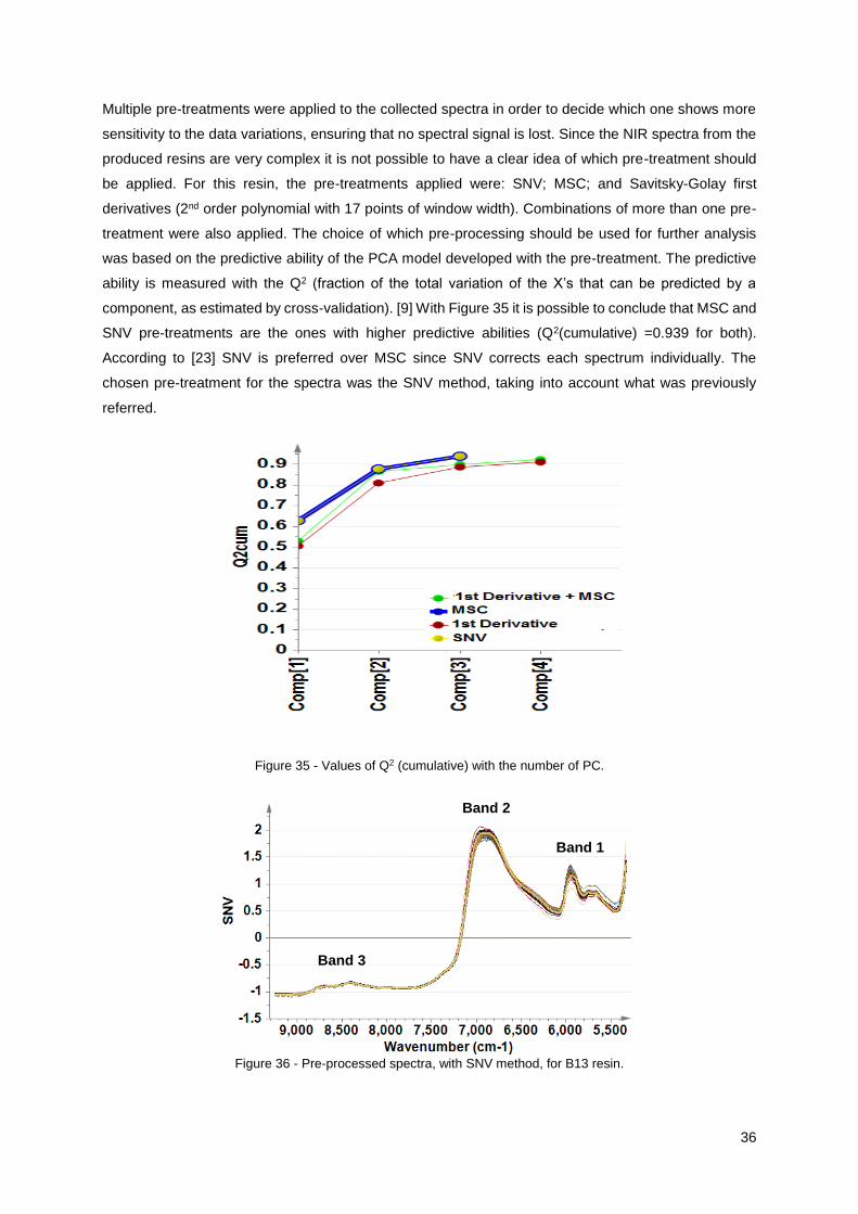
36
Multiple pre-treatments were applied to the collected spectra in order to decide which one shows more
sensitivity to the data variations, ensuring that no spectral signal is lost. Since the NIR spectra from the
produced resins are very complex it is not possible to have a clear idea of which pre-treatment should
be applied. For this resin, the pre-treatments applied were: SNV; MSC; and Savitsky-Golay first
derivatives (2nd order polynomial with 17 points of window width). Combinations of more than one pre-
treatment were also applied. The choice of which pre-processing should be used for further analysis
was based on the predictive ability of the PCA model developed with the pre-treatment. The predictive
ability is measured with the Q2 (fraction of the total variation of the X’s that can be predicted by a
component, as estimated by cross-validation). [9] With Figure 35 it is possible to conclude that MSC and
SNV pre-treatments are the ones with higher predictive abilities (Q2(cumulative) =0.939 for both).
According to [23] SNV is preferred over MSC since SNV corrects each spectrum individually. The
chosen pre-treatment for the spectra was the SNV method, taking into account what was previously
referred.
Figure 35 - Values of Q2 (cumulative) with the number of PC.
Figure 36 - Pre-processed spectra, with SNV method, for B13 resin.
Band 1
Band 2
Band 3
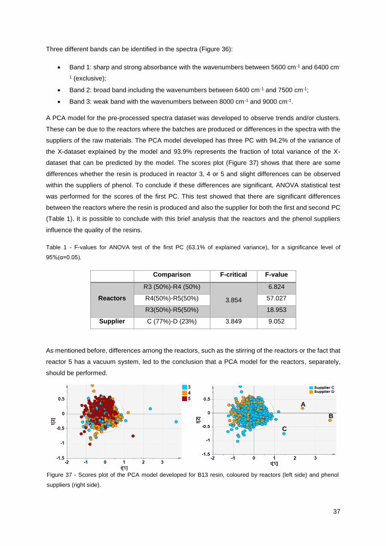
37
Three different bands can be identified in the spectra (Figure 36):
Band 1: sharp and strong absorbance with the wavenumbers between 5600 cm-1 and 6400 cm-
1 (exclusive);
Band 2: broad band including the wavenumbers between 6400 cm-1 and 7500 cm-1;
Band 3: weak band with the wavenumbers between 8000 cm-1 and 9000 cm-1.
A PCA model for the pre-processed spectra dataset was developed to observe trends and/or clusters.
These can be due to the reactors where the batches are produced or differences in the spectra with the
suppliers of the raw materials. The PCA model developed has three PC with 94.2% of the variance of
the X-dataset explained by the model and 93.9% represents the fraction of total variance of the X-
dataset that can be predicted by the model. The scores plot (Figure 37) shows that there are some
differences whether the resin is produced in reactor 3, 4 or 5 and slight differences can be observed
within the suppliers of phenol. To conclude if these differences are significant, ANOVA statistical test
was performed for the scores of the first PC. This test showed that there are significant differences
between the reactors where the resin is produced and also the supplier for both the first and second PC
(Table 1). It is possible to conclude with this brief analysis that the reactors and the phenol suppliers
influence the quality of the resins.
Table 1 - F-values for ANOVA test of the first PC (63.1% of explained variance), for a significance level of
95%(α=0.05).
Comparison F-critical F-value
Reactors
R3 (50%)-R4 (50%)
3.854
6.824
R4(50%)-R5(50%) 57.027
R3(50%)-R5(50%) 18.953
Supplier C (77%)-D (23%) 3.849 9.052
As mentioned before, differences among the reactors, such as the stirring of the reactors or the fact that
reactor 5 has a vacuum system, led to the conclusion that a PCA model for the reactors, separately,
should be performed.
Figure 37 - Scores plot of the PCA model developed for B13 resin, coloured by reactors (left side) and phenol
suppliers (right side).
A
B
C
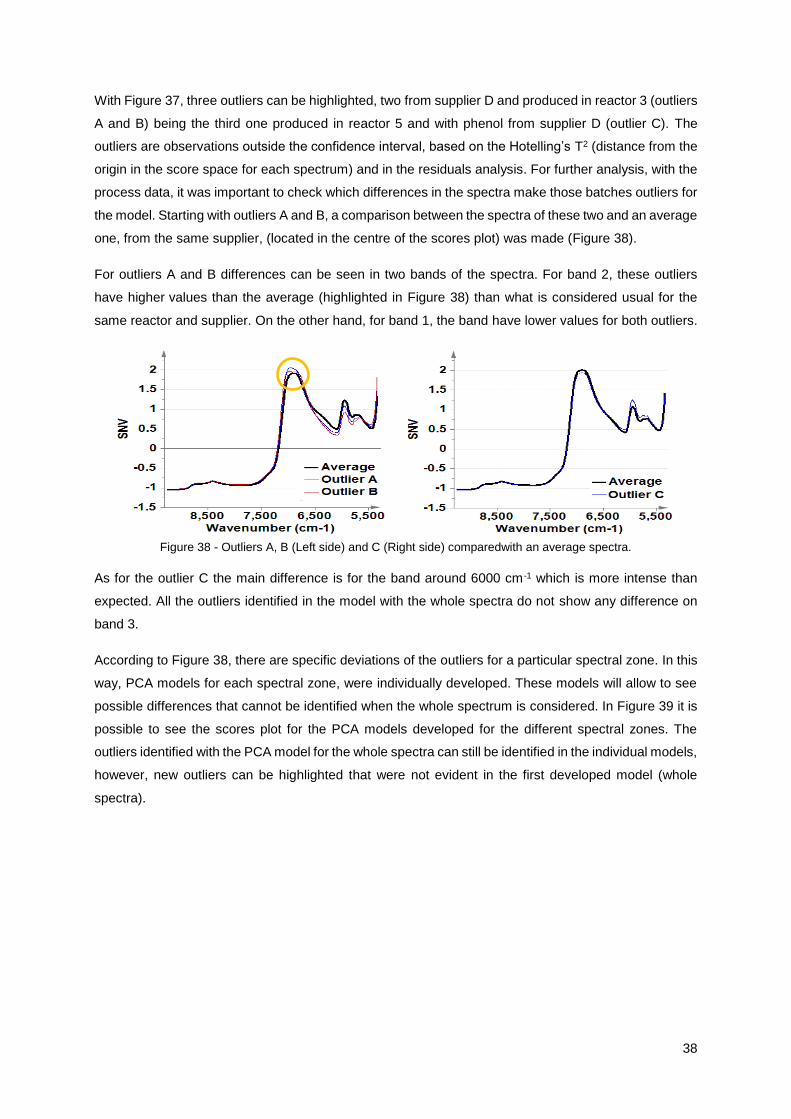
38
With Figure 37, three outliers can be highlighted, two from supplier D and produced in reactor 3 (outliers
A and B) being the third one produced in reactor 5 and with phenol from supplier D (outlier C). The
outliers are observations outside the confidence interval, based on the Hotelling’s T2 (distance from the
origin in the score space for each spectrum) and in the residuals analysis. For further analysis, with the
process data, it was important to check which differences in the spectra make those batches outliers for
the model. Starting with outliers A and B, a comparison between the spectra of these two and an average
one, from the same supplier, (located in the centre of the scores plot) was made (Figure 38).
For outliers A and B differences can be seen in two bands of the spectra. For band 2, these outliers
have higher values than the average (highlighted in Figure 38) than what is considered usual for the
same reactor and supplier. On the other hand, for band 1, the band have lower values for both outliers.
As for the outlier C the main difference is for the band around 6000 cm -1 which is more intense than
expected. All the outliers identified in the model with the whole spectra do not show any difference on
band 3.
According to Figure 38, there are specific deviations of the outliers for a particular spectral zone. In this
way, PCA models for each spectral zone, were individually developed. These models will allow to see
possible differences that cannot be identified when the whole spectrum is considered. In Figure 39 it is
possible to see the scores plot for the PCA models developed for the different spectral zones. The
outliers identified with the PCA model for the whole spectra can still be identified in the individual models,
however, new outliers can be highlighted that were not evident in the first developed model (whole
spectra).
Figure 38 - Outliers A, B (Left side) and C (Right side) comparedwith an average spectra.
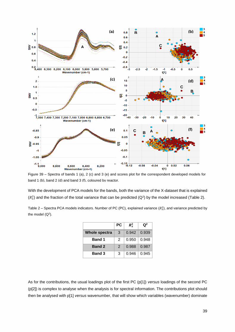
39
With the development of PCA models for the bands, both the variance of the X-dataset that is explained
(𝑅𝑥2) and the fraction of the total variance that can be predicted (Q2) by the model increased (Table 2).
Table 2 – Spectra PCA models indicators. Number of PC (PC), explained variance (𝑅𝑥2), and variance predicted by
the model (Q2).
PC 𝑹𝒙𝟐 Q2
Whole spectra 3 0.942 0.939
Band 1 2 0.950 0.948
Band 2 2 0.988 0.987
Band 3 3 0.946 0.945
As for the contributions, the usual loadings plot of the first PC (p[1]) versus loadings of the second PC
(p[2]) is complex to analyse when the analysis is for spectral information. The contributions plot should
then be analysed with p[1] versus wavenumber, that will show which variables (wavenumber) dominate
A B
C
A B C
(a) (b)
(c) (d)
(e) (f)
A
B C
Figure 39 – Spectra of bands 1 (a), 2 (c) and 3 (e) and scores plot for the correspondent developed models for
band 1 (b), band 2 (d) and band 3 (f), coloured by reactor.
A
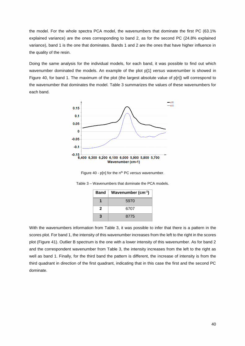
40
the model. For the whole spectra PCA model, the wavenumbers that dominate the first PC (63.1%
explained variance) are the ones corresponding to band 2, as for the second PC (24.8% explained
variance), band 1 is the one that dominates. Bands 1 and 2 are the ones that have higher influence in
the quality of the resin.
Doing the same analysis for the individual models, for each band, it was possible to find out which
wavenumber dominated the models. An example of the plot p[1] versus wavenumber is showed in
Figure 40, for band 1. The maximum of the plot (the largest absolute value of p[n]) will correspond to
the wavenumber that dominates the model. Table 3 summarizes the values of these wavenumbers for
each band.
Figure 40 - p[n] for the nth PC versus wavenumber.
Table 3 – Wavenumbers that dominate the PCA models.
With the wavenumbers information from Table 3, it was possible to infer that there is a pattern in the
scores plot. For band 1, the intensity of this wavenumber increases from the left to the right in the scores
plot (Figure 41). Outlier B spectrum is the one with a lower intensity of this wavenumber. As for band 2
and the correspondent wavenumber from Table 3, the intensity increases from the left to the right as
well as band 1. Finally, for the third band the pattern is different, the increase of intensity is from the
third quadrant in direction of the first quadrant, indicating that in this case the first and the second PC
dominate.
Band Wavenumber (cm-1)
1 5970
2 6707
3 8775
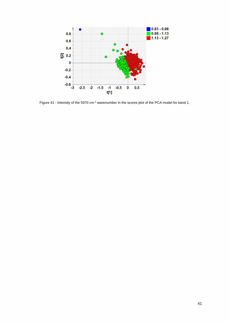
41
Figure 41 - Intensity of the 5970 cm-1 wavenumber in the scores plot of the PCA model for band 1.
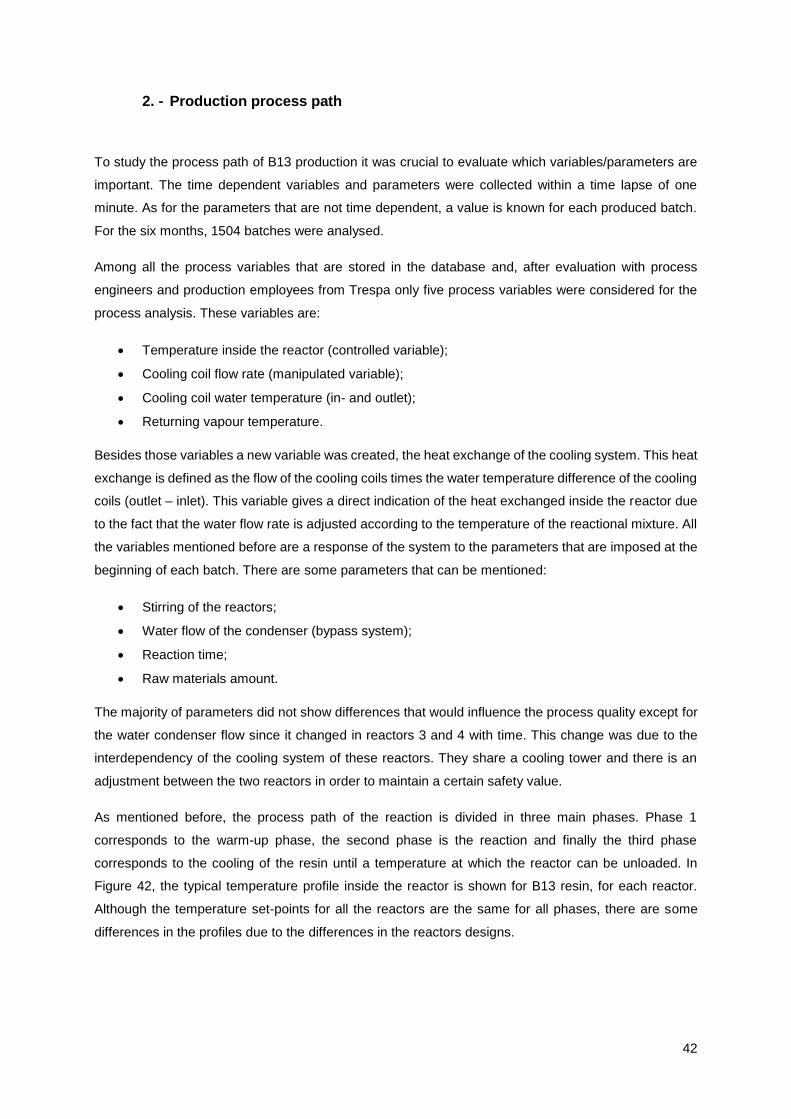
42
2. - Production process path
To study the process path of B13 production it was crucial to evaluate which variables/parameters are
important. The time dependent variables and parameters were collected within a time lapse of one
minute. As for the parameters that are not time dependent, a value is known for each produced batch.
For the six months, 1504 batches were analysed.
Among all the process variables that are stored in the database and, after evaluation with process
engineers and production employees from Trespa only five process variables were considered for the
process analysis. These variables are:
Temperature inside the reactor (controlled variable);
Cooling coil flow rate (manipulated variable);
Cooling coil water temperature (in- and outlet);
Returning vapour temperature.
Besides those variables a new variable was created, the heat exchange of the cooling system. This heat
exchange is defined as the flow of the cooling coils times the water temperature difference of the cooling
coils (outlet – inlet). This variable gives a direct indication of the heat exchanged inside the reactor due
to the fact that the water flow rate is adjusted according to the temperature of the reactional mixture. All
the variables mentioned before are a response of the system to the parameters that are imposed at the
beginning of each batch. There are some parameters that can be mentioned:
Stirring of the reactors;
Water flow of the condenser (bypass system);
Reaction time;
Raw materials amount.
The majority of parameters did not show differences that would influence the process quality except for
the water condenser flow since it changed in reactors 3 and 4 with time. This change was due to the
interdependency of the cooling system of these reactors. They share a cooling tower and there is an
adjustment between the two reactors in order to maintain a certain safety value.
As mentioned before, the process path of the reaction is divided in three main phases. Phase 1
corresponds to the warm-up phase, the second phase is the reaction and finally the third phase
corresponds to the cooling of the resin until a temperature at which the reactor can be unloaded. In
Figure 42, the typical temperature profile inside the reactor is shown for B13 resin, for each reactor.
Although the temperature set-points for all the reactors are the same for all phases, there are some
differences in the profiles due to the differences in the reactors designs.
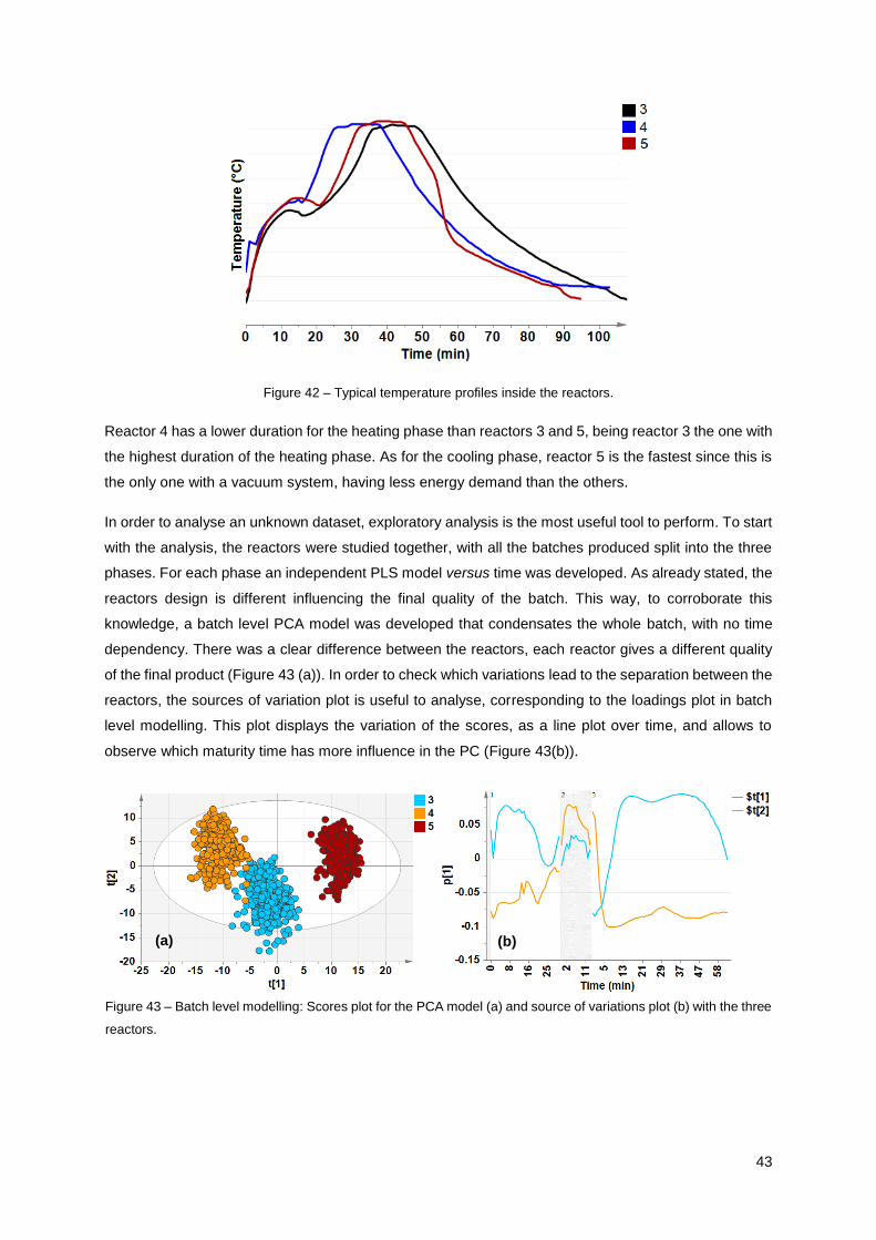
43
Figure 42 – Typical temperature profiles inside the reactors.
Reactor 4 has a lower duration for the heating phase than reactors 3 and 5, being reactor 3 the one with
the highest duration of the heating phase. As for the cooling phase, reactor 5 is the fastest since this is
the only one with a vacuum system, having less energy demand than the others.
In order to analyse an unknown dataset, exploratory analysis is the most useful tool to perform. To start
with the analysis, the reactors were studied together, with all the batches produced split into the three
phases. For each phase an independent PLS model versus time was developed. As already stated, the
reactors design is different influencing the final quality of the batch. This way, to corroborate this
knowledge, a batch level PCA model was developed that condensates the whole batch, with no time
dependency. There was a clear difference between the reactors, each reactor gives a different quality
of the final product (Figure 43 (a)). In order to check which variations lead to the separation between the
reactors, the sources of variation plot is useful to analyse, corresponding to the loadings plot in batch
level modelling. This plot displays the variation of the scores, as a line plot over time, and allows to
observe which maturity time has more influence in the PC (Figure 43(b)).
(a) (b)
Figure 43 – Batch level modelling: Scores plot for the PCA model (a) and source of variations plot (b) with the three
reactors.
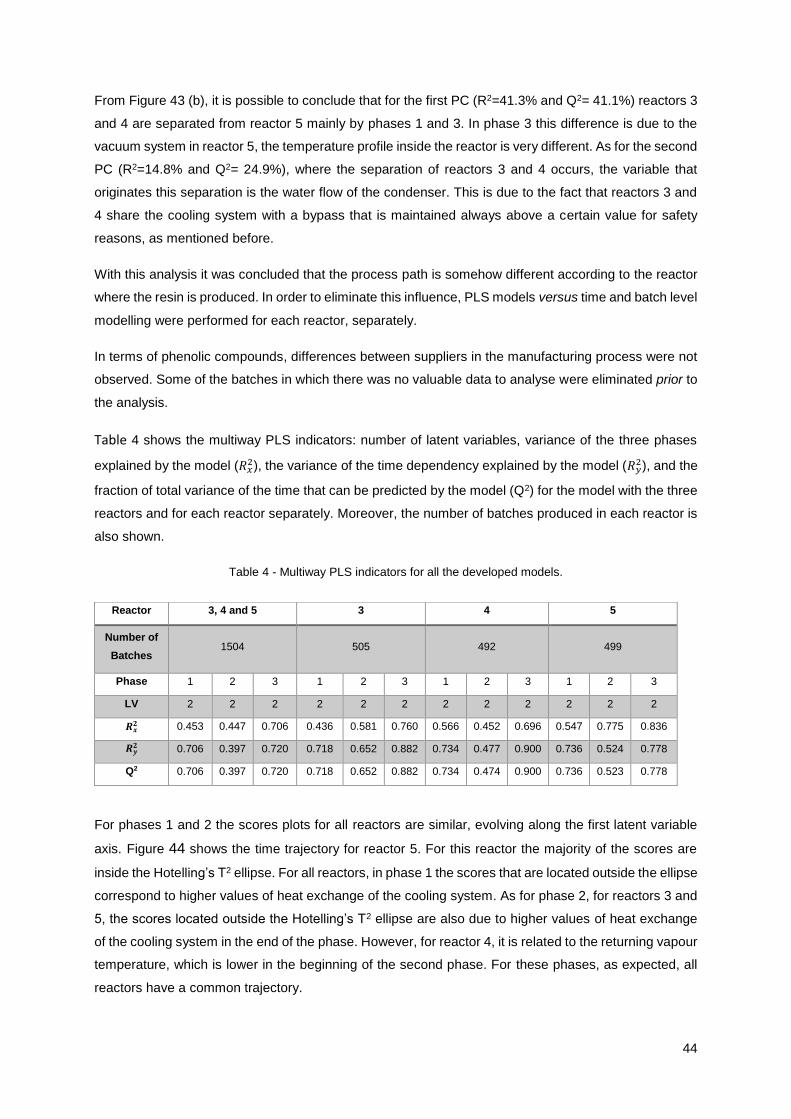
44
From Figure 43 (b), it is possible to conclude that for the first PC (R2=41.3% and Q2= 41.1%) reactors 3
and 4 are separated from reactor 5 mainly by phases 1 and 3. In phase 3 this difference is due to the
vacuum system in reactor 5, the temperature profile inside the reactor is very different. As for the second
PC (R2=14.8% and Q2= 24.9%), where the separation of reactors 3 and 4 occurs, the variable that
originates this separation is the water flow of the condenser. This is due to the fact that reactors 3 and
4 share the cooling system with a bypass that is maintained always above a certain value for safety
reasons, as mentioned before.
With this analysis it was concluded that the process path is somehow different according to the reactor
where the resin is produced. In order to eliminate this influence, PLS models versus time and batch level
modelling were performed for each reactor, separately.
In terms of phenolic compounds, differences between suppliers in the manufacturing process were not
observed. Some of the batches in which there was no valuable data to analyse were eliminated prior to
the analysis.
Table 4 shows the multiway PLS indicators: number of latent variables, variance of the three phases
explained by the model (𝑅𝑥2), the variance of the time dependency explained by the model (𝑅𝑦
2), and the
fraction of total variance of the time that can be predicted by the model (Q2) for the model with the three
reactors and for each reactor separately. Moreover, the number of batches produced in each reactor is
also shown.
Table 4 - Multiway PLS indicators for all the developed models.
For phases 1 and 2 the scores plots for all reactors are similar, evolving along the first latent variable
axis. Figure 44 shows the time trajectory for reactor 5. For this reactor the majority of the scores are
inside the Hotelling’s T2 ellipse. For all reactors, in phase 1 the scores that are located outside the ellipse
correspond to higher values of heat exchange of the cooling system. As for phase 2, for reactors 3 and
5, the scores located outside the Hotelling’s T2 ellipse are also due to higher values of heat exchange
of the cooling system in the end of the phase. However, for reactor 4, it is related to the returning vapour
temperature, which is lower in the beginning of the second phase. For these phases, as expected, all
reactors have a common trajectory.
Reactor 3, 4 and 5 3 4 5
Number of
Batches 1504 505 492 499
Phase 1 2 3 1 2 3 1 2 3 1 2 3
LV 2 2 2 2 2 2 2 2 2 2 2 2
𝑹𝒙𝟐 0.453 0.447 0.706 0.436 0.581 0.760 0.566 0.452 0.696 0.547 0.775 0.836
𝑹𝒚𝟐 0.706 0.397 0.720 0.718 0.652 0.882 0.734 0.477 0.900 0.736 0.524 0.778
Q2 0.706 0.397 0.720 0.718 0.652 0.882 0.734 0.474 0.900 0.736 0.523 0.778
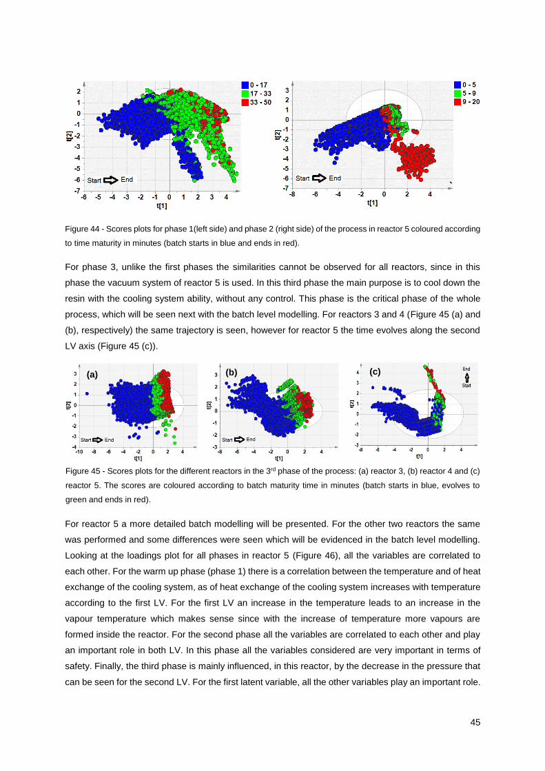
45
Figure 44 - Scores plots for phase 1(left side) and phase 2 (right side) of the process in reactor 5 coloured according
to time maturity in minutes (batch starts in blue and ends in red).
For phase 3, unlike the first phases the similarities cannot be observed for all reactors, since in this
phase the vacuum system of reactor 5 is used. In this third phase the main purpose is to cool down the
resin with the cooling system ability, without any control. This phase is the critical phase of the whole
process, which will be seen next with the batch level modelling. For reactors 3 and 4 (Figure 45 (a) and
(b), respectively) the same trajectory is seen, however for reactor 5 the time evolves along the second
LV axis (Figure 45 (c)).
For reactor 5 a more detailed batch modelling will be presented. For the other two reactors the same
was performed and some differences were seen which will be evidenced in the batch level modelling.
Looking at the loadings plot for all phases in reactor 5 (Figure 46), all the variables are correlated to
each other. For the warm up phase (phase 1) there is a correlation between the temperature and of heat
exchange of the cooling system, as of heat exchange of the cooling system increases with temperature
according to the first LV. For the first LV an increase in the temperature leads to an increase in the
vapour temperature which makes sense since with the increase of temperature more vapours are
formed inside the reactor. For the second phase all the variables are correlated to each other and play
an important role in both LV. In this phase all the variables considered are very important in terms of
safety. Finally, the third phase is mainly influenced, in this reactor, by the decrease in the pressure that
can be seen for the second LV. For the first latent variable, all the other variables play an important role.
(a) (b) (c)
Figure 45 - Scores plots for the different reactors in the 3rd phase of the process: (a) reactor 3, (b) reactor 4 and (c)
reactor 5. The scores are coloured according to batch maturity time in minutes (batch starts in blue, evolves to
green and ends in red).
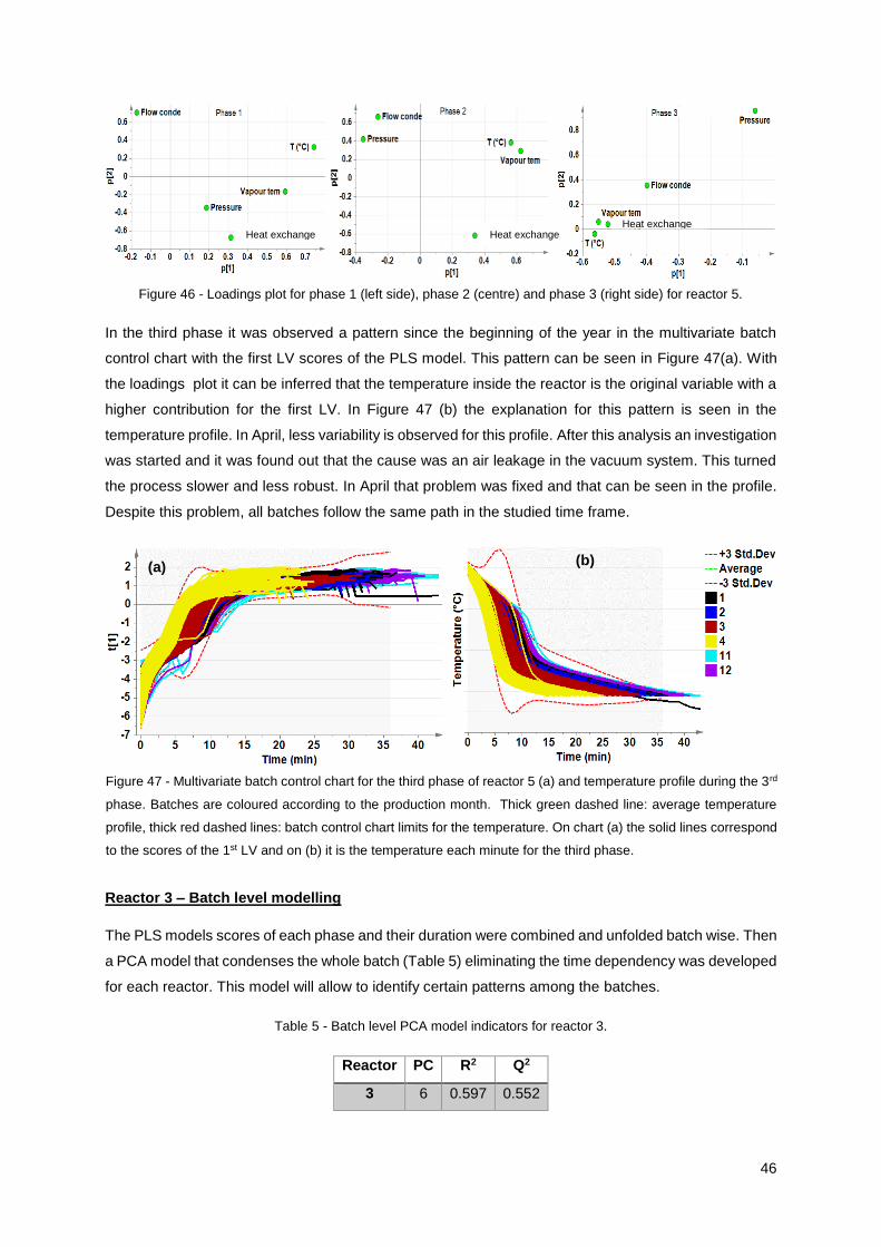
46
In the third phase it was observed a pattern since the beginning of the year in the multivariate batch
control chart with the first LV scores of the PLS model. This pattern can be seen in Figure 47(a). With
the loadings plot it can be inferred that the temperature inside the reactor is the original variable with a
higher contribution for the first LV. In Figure 47 (b) the explanation for this pattern is seen in the
temperature profile. In April, less variability is observed for this profile. After this analysis an investigation
was started and it was found out that the cause was an air leakage in the vacuum system. This turned
the process slower and less robust. In April that problem was fixed and that can be seen in the profile.
Despite this problem, all batches follow the same path in the studied time frame.
Reactor 3 – Batch level modelling
The PLS models scores of each phase and their duration were combined and unfolded batch wise. Then
a PCA model that condenses the whole batch (Table 5) eliminating the time dependency was developed
for each reactor. This model will allow to identify certain patterns among the batches.
Table 5 - Batch level PCA model indicators for reactor 3.
Reactor PC R2 Q2
3 6 0.597 0.552
Figure 46 - Loadings plot for phase 1 (left side), phase 2 (centre) and phase 3 (right side) for reactor 5.
Figure 47 - Multivariate batch control chart for the third phase of reactor 5 (a) and temperature profile during the 3rd
phase. Batches are coloured according to the production month. Thick green dashed line: average temperature
profile, thick red dashed lines: batch control chart limits for the temperature. On chart (a) the solid lines correspond
to the scores of the 1st LV and on (b) it is the temperature each minute for the third phase.
(b) (a)
Heat exchange Heat exchange Heat exchange
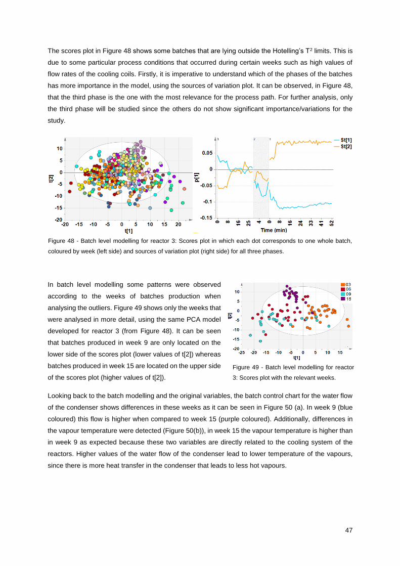
47
The scores plot in Figure 48 shows some batches that are lying outside the Hotelling’s T2 limits. This is
due to some particular process conditions that occurred during certain weeks such as high values of
flow rates of the cooling coils. Firstly, it is imperative to understand which of the phases of the batches
has more importance in the model, using the sources of variation plot. It can be observed, in Figure 48,
that the third phase is the one with the most relevance for the process path. For further analysis, only
the third phase will be studied since the others do not show significant importance/variations for the
study.
In batch level modelling some patterns were observed
according to the weeks of batches production when
analysing the outliers. Figure 49 shows only the weeks that
were analysed in more detail, using the same PCA model
developed for reactor 3 (from Figure 48). It can be seen
that batches produced in week 9 are only located on the
lower side of the scores plot (lower values of t[2]) whereas
batches produced in week 15 are located on the upper side
of the scores plot (higher values of t[2]).
Looking back to the batch modelling and the original variables, the batch control chart for the water flow
of the condenser shows differences in these weeks as it can be seen in Figure 50 (a). In week 9 (blue
coloured) this flow is higher when compared to week 15 (purple coloured). Additionally, differences in
the vapour temperature were detected (Figure 50(b)), in week 15 the vapour temperature is higher than
in week 9 as expected because these two variables are directly related to the cooling system of the
reactors. Higher values of the water flow of the condenser lead to lower temperature of the vapours,
since there is more heat transfer in the condenser that leads to less hot vapours.
Figure 49 - Batch level modelling for reactor
3: Scores plot with the relevant weeks.
Figure 48 - Batch level modelling for reactor 3: Scores plot in which each dot corresponds to one whole batch,
coloured by week (left side) and sources of variation plot (right side) for all three phases.
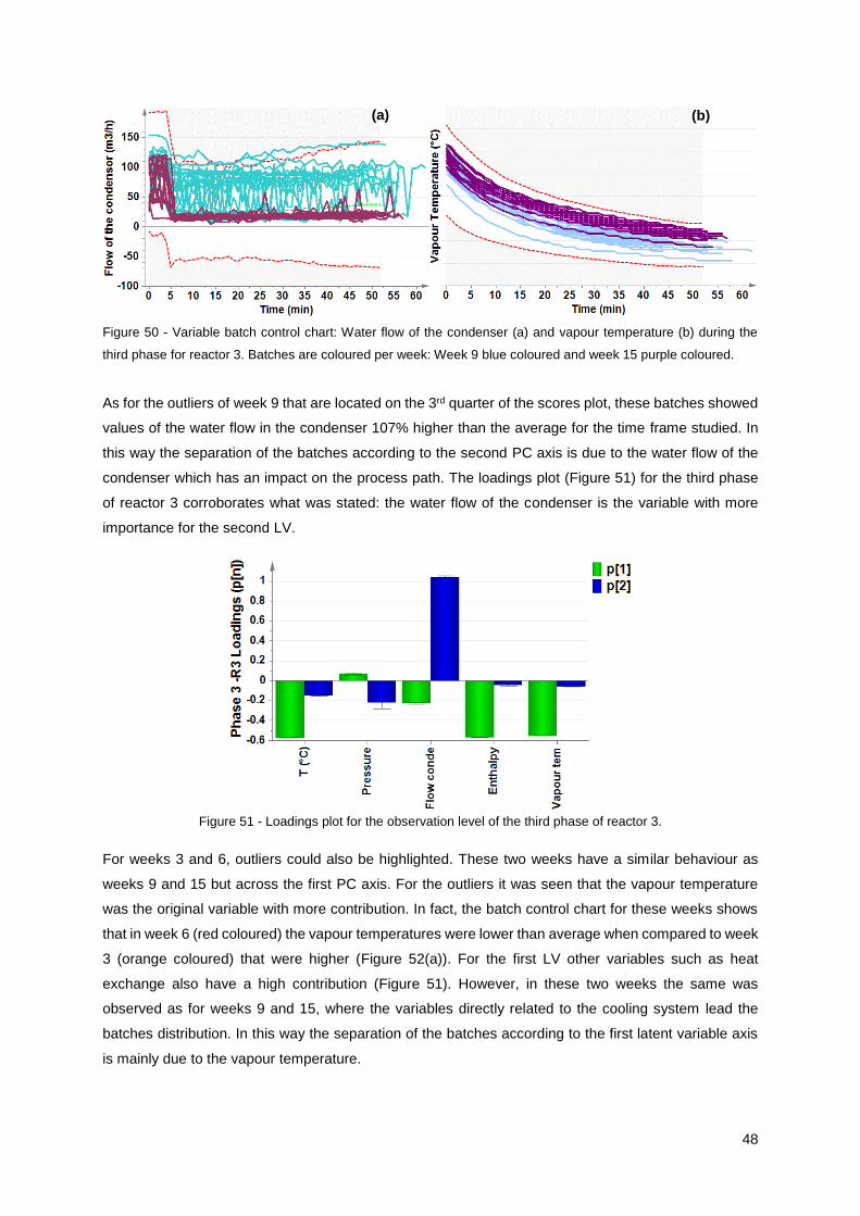
48
As for the outliers of week 9 that are located on the 3rd quarter of the scores plot, these batches showed
values of the water flow in the condenser 107% higher than the average for the time frame studied. In
this way the separation of the batches according to the second PC axis is due to the water flow of the
condenser which has an impact on the process path. The loadings plot (Figure 51) for the third phase
of reactor 3 corroborates what was stated: the water flow of the condenser is the variable with more
importance for the second LV.
Figure 51 - Loadings plot for the observation level of the third phase of reactor 3.
For weeks 3 and 6, outliers could also be highlighted. These two weeks have a similar behaviour as
weeks 9 and 15 but across the first PC axis. For the outliers it was seen that the vapour temperature
was the original variable with more contribution. In fact, the batch control chart for these weeks shows
that in week 6 (red coloured) the vapour temperatures were lower than average when compared to week
3 (orange coloured) that were higher (Figure 52(a)). For the first LV other variables such as heat
exchange also have a high contribution (Figure 51). However, in these two weeks the same was
observed as for weeks 9 and 15, where the variables directly related to the cooling system lead the
batches distribution. In this way the separation of the batches according to the first latent variable axis
is mainly due to the vapour temperature.
Figure 50 - Variable batch control chart: Water flow of the condenser (a) and vapour temperature (b) during the
third phase for reactor 3. Batches are coloured per week: Week 9 blue coloured and week 15 purple coloured.
(b) (a)
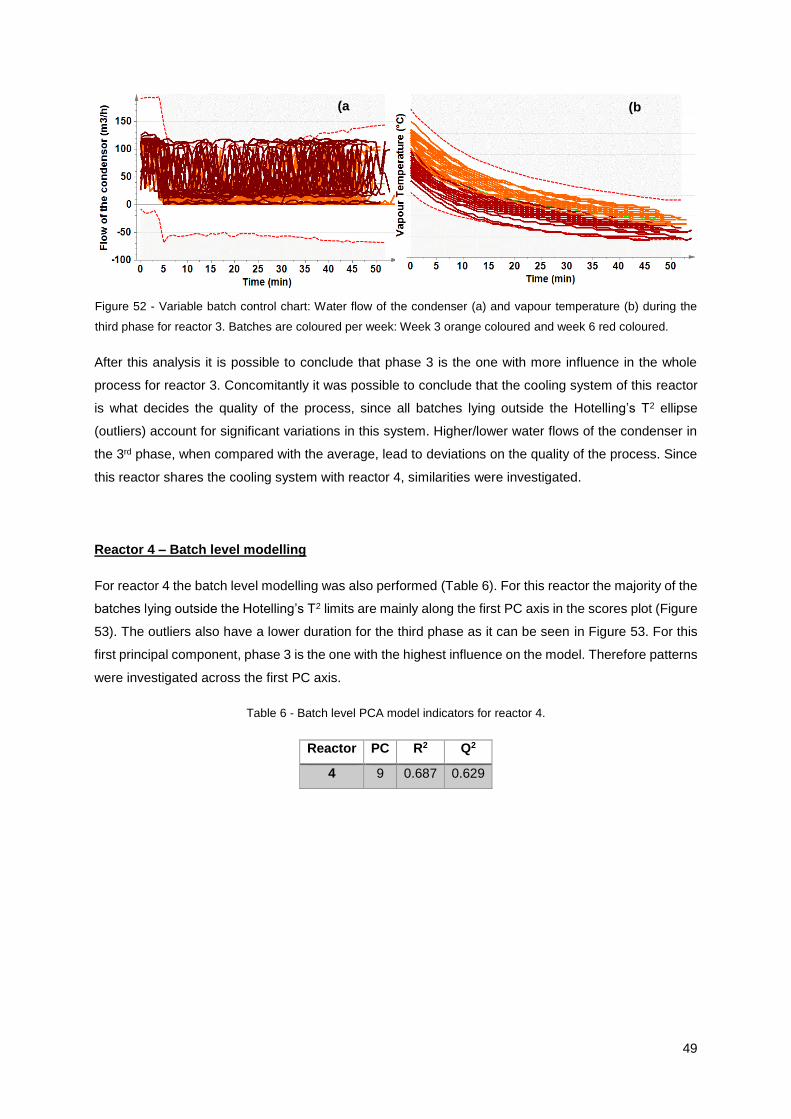
49
After this analysis it is possible to conclude that phase 3 is the one with more influence in the whole
process for reactor 3. Concomitantly it was possible to conclude that the cooling system of this reactor
is what decides the quality of the process, since all batches lying outside the Hotelling’s T2 ellipse
(outliers) account for significant variations in this system. Higher/lower water flows of the condenser in
the 3rd phase, when compared with the average, lead to deviations on the quality of the process. Since
this reactor shares the cooling system with reactor 4, similarities were investigated.
Reactor 4 – Batch level modelling
For reactor 4 the batch level modelling was also performed (Table 6). For this reactor the majority of the
batches lying outside the Hotelling’s T2 limits are mainly along the first PC axis in the scores plot (Figure
53). The outliers also have a lower duration for the third phase as it can be seen in Figure 53. For this
first principal component, phase 3 is the one with the highest influence on the model. Therefore patterns
were investigated across the first PC axis.
Table 6 - Batch level PCA model indicators for reactor 4.
Reactor PC R2 Q2
4 9 0.687 0.629
Figure 52 - Variable batch control chart: Water flow of the condenser (a) and vapour temperature (b) during the
third phase for reactor 3. Batches are coloured per week: Week 3 orange coloured and week 6 red coloured.
(b(a
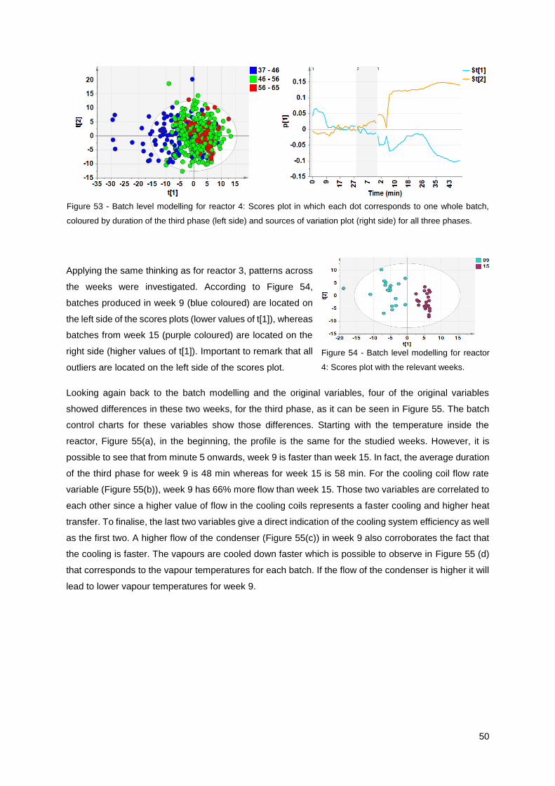
50
Applying the same thinking as for reactor 3, patterns across
the weeks were investigated. According to Figure 54,
batches produced in week 9 (blue coloured) are located on
the left side of the scores plots (lower values of t[1]), whereas
batches from week 15 (purple coloured) are located on the
right side (higher values of t[1]). Important to remark that all
outliers are located on the left side of the scores plot.
Looking again back to the batch modelling and the original variables, four of the original variables
showed differences in these two weeks, for the third phase, as it can be seen in Figure 55. The batch
control charts for these variables show those differences. Starting with the temperature inside the
reactor, Figure 55(a), in the beginning, the profile is the same for the studied weeks. However, it is
possible to see that from minute 5 onwards, week 9 is faster than week 15. In fact, the average duration
of the third phase for week 9 is 48 min whereas for week 15 is 58 min. For the cooling coil flow rate
variable (Figure 55(b)), week 9 has 66% more flow than week 15. Those two variables are correlated to
each other since a higher value of flow in the cooling coils represents a faster cooling and higher heat
transfer. To finalise, the last two variables give a direct indication of the cooling system efficiency as well
as the first two. A higher flow of the condenser (Figure 55(c)) in week 9 also corroborates the fact that
the cooling is faster. The vapours are cooled down faster which is possible to observe in Figure 55 (d)
that corresponds to the vapour temperatures for each batch. If the flow of the condenser is higher it will
lead to lower vapour temperatures for week 9.
Figure 53 - Batch level modelling for reactor 4: Scores plot in which each dot corresponds to one whole batch,
coloured by duration of the third phase (left side) and sources of variation plot (right side) for all three phases.
Figure 54 - Batch level modelling for reactor
4: Scores plot with the relevant weeks.
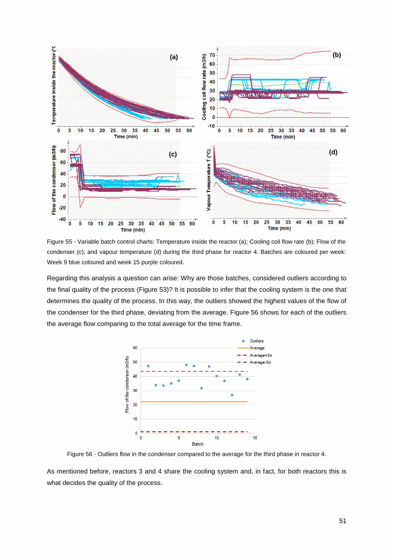
51
Regarding this analysis a question can arise: Why are those batches, considered outliers according to
the final quality of the process (Figure 53)? It is possible to infer that the cooling system is the one that
determines the quality of the process. In this way, the outliers showed the highest values of the flow of
the condenser for the third phase, deviating from the average. Figure 56 shows for each of the outliers
the average flow comparing to the total average for the time frame.
Figure 56 - Outliers flow in the condenser compared to the average for the third phase in reactor 4.
As mentioned before, reactors 3 and 4 share the cooling system and, in fact, for both reactors this is
what decides the quality of the process.
(a) (b)
(c) (d)
Figure 55 - Variable batch control charts: Temperature inside the reactor (a); Cooling coil flow rate (b); Flow of the
condenser (c); and vapour temperature (d) during the third phase for reactor 4. Batches are coloured per week:
Week 9 blue coloured and week 15 purple coloured.
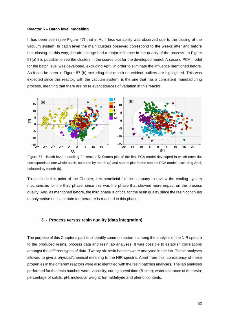
52
Reactor 5 – Batch level modelling
It has been seen (see Figure 47) that in April less variability was observed due to the closing of the
vacuum system. In batch level the main clusters observed correspond to the weeks after and before
that closing. In this way, the air leakage had a major influence in the quality of the process. In Figure
57(a) it is possible to see the clusters in the scores plot for the developed model. A second PCA model
for the batch level was developed, excluding April, in order to eliminate the influence mentioned before.
As it can be seen in Figure 57 (b) excluding that month no evident outliers are highlighted. This was
expected since this reactor, with the vacuum system, is the one that has a consistent manufacturing
process, meaning that there are no relevant sources of variation in this reactor.
To conclude this point of the Chapter, it is beneficial for the company to review the cooling system
mechanisms for the third phase, since this was the phase that showed more impact on the process
quality. And, as mentioned before, the third phase is critical for the resin quality since the resin continues
to polymerise until a certain temperature is reached in this phase.
3. - Process versus resin quality (data integration)
The purpose of this Chapter’s part is to identify common patterns among the analysis of the NIR spectra
to the produced resins, process data and resin lab analyses. It was possible to establish correlations
amongst the different types of data. Twenty-six resin batches were analysed in the lab. These analyses
allowed to give a physical/chemical meaning to the NIR spectra. Apart from this, consistency of these
properties in the different reactors were also identified with the resin batches analyses. The lab analyses
performed for the resin batches were: viscosity; curing speed time (B-time); water tolerance of the resin;
percentage of solids; pH; molecular weight; formaldehyde and phenol contents.
Figure 57 - Batch level modelling for reactor 5: Scores plot of the first PCA model developed in which each dot
corresponds to one whole batch, coloured by month (a) and scores plot for the second PCA model, excluding April,
coloured by month (b).
(a) (b)
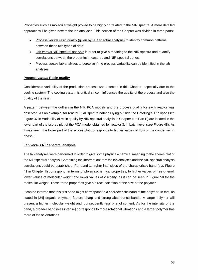
53
Properties such as molecular weight proved to be highly correlated to the NIR spectra. A more detailed
approach will be given next to the lab analyses. This section of the Chapter was divided in three parts:
Process versus resin quality (given by NIR spectral analysis) to identify common patterns
between these two types of data;
Lab versus NIR spectral analysis in order to give a meaning to the NIR spectra and quantify
correlations between the properties measured and NIR spectral zones;
Process versus lab analyses to perceive if the process variability can be identified in the lab
analyses.
Process versus Resin quality
Considerable variability of the production process was detected in this Chapter, especially due to the
cooling system. The cooling system is critical since it influences the quality of the process and also the
quality of the resin.
A pattern between the outliers in the NIR PCA models and the process quality for each reactor was
observed. As an example, for reactor 3, all spectra batches lying outside the Hotelling’s T2 ellipse (see
Figure 37 in Variability of resin quality by NIR spectral analysis of Chapter II of Part B) are located in the
lower part of the scores plot of the PCA model obtained for reactor 3, in batch level (see Figure 48). As
it was seen, the lower part of the scores plot corresponds to higher values of flow of the condenser in
phase 3.
Lab versus NIR spectral analysis
The lab analyses were performed in order to give some physical/chemical meaning to the scores plot of
the NIR spectral analysis. Combining the information from the lab analyses and the NIR spectral analysis
correlations could be established. For band 1, higher intensities of the characteristic band (see Figure
41 in Chapter II) correspond, in terms of physical/chemical properties, to higher values of free-phenol,
lower values of molecular weight and lower values of viscosity, as it can be seen in Figure 58 for the
molecular weight. These three properties give a direct indication of the size of the polymer.
It can be inferred that this first band might correspond to a characteristic band of the polymer. In fact, as
stated in [24] organic polymers feature sharp and strong absorbance bands. A larger polymer will
present a higher molecular weight and, consequently less phenol content. As for the intensity of the
band, a broader band (less intense) corresponds to more rotational vibrations and a larger polymer has
more of these vibrations.
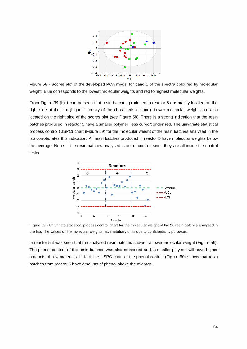
54
Figure 58 - Scores plot of the developed PCA model for band 1 of the spectra coloured by molecular
weight. Blue corresponds to the lowest molecular weights and red to highest molecular weights.
From Figure 39 (b) it can be seen that resin batches produced in reactor 5 are mainly located on the
right side of the plot (higher intensity of the characteristic band). Lower molecular weights are also
located on the right side of the scores plot (see Figure 58). There is a strong indication that the resin
batches produced in reactor 5 have a smaller polymer, less cured/condensed. The univariate statistical
process control (USPC) chart (Figure 59) for the molecular weight of the resin batches analysed in the
lab corroborates this indication. All resin batches produced in reactor 5 have molecular weights below
the average. None of the resin batches analysed is out of control, since they are all inside the control
limits.
In reactor 5 it was seen that the analysed resin batches showed a lower molecular weight (Figure 59).
The phenol content of the resin batches was also measured and, a smaller polymer will have higher
amounts of raw materials. In fact, the USPC chart of the phenol content (Figure 60) shows that resin
batches from reactor 5 have amounts of phenol above the average.
Figure 59 - Univariate statistical process control chart for the molecular weight of the 26 resin batches analysed in
the lab. The values of the molecular weights have arbitrary units due to confidentiality purposes.
Reactors
3 4 5
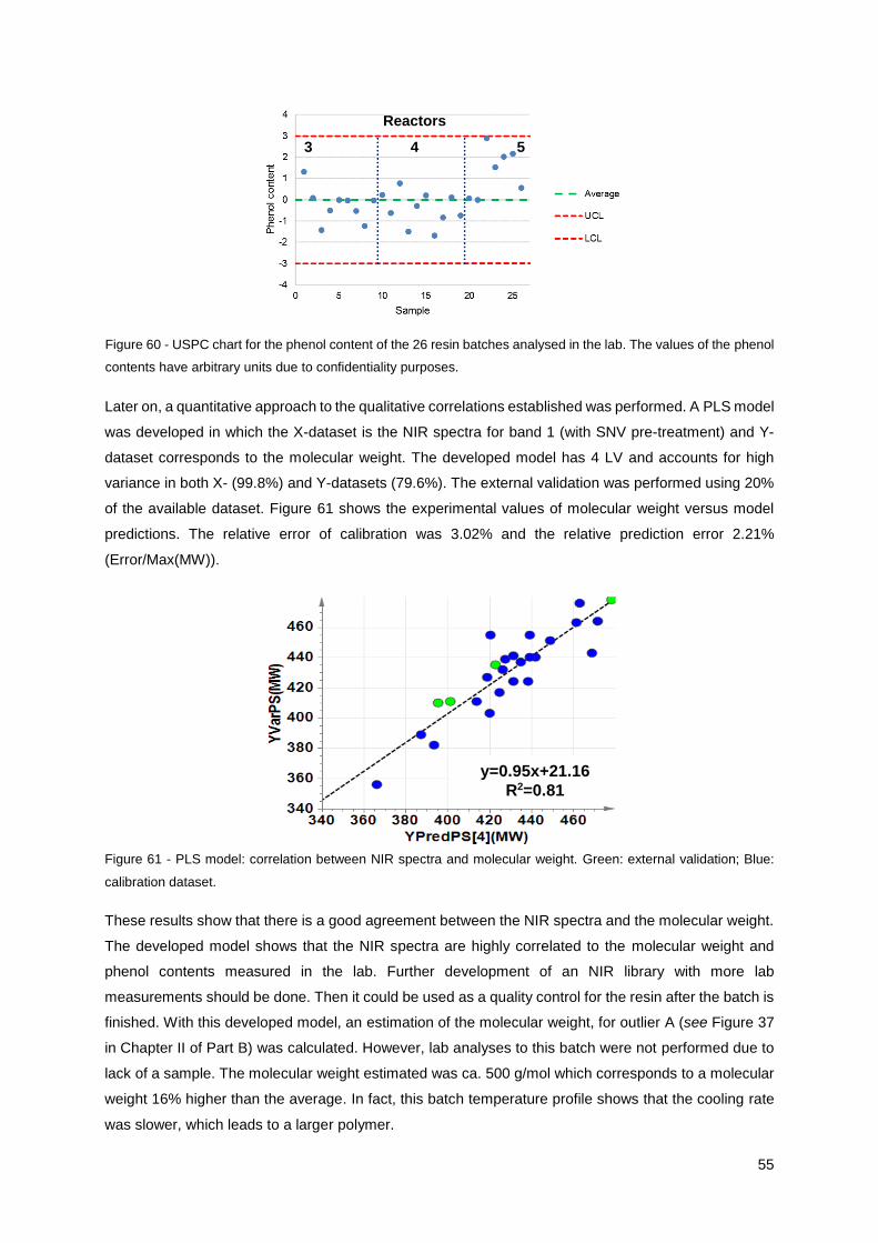
55
Later on, a quantitative approach to the qualitative correlations established was performed. A PLS model
was developed in which the X-dataset is the NIR spectra for band 1 (with SNV pre-treatment) and Y-
dataset corresponds to the molecular weight. The developed model has 4 LV and accounts for high
variance in both X- (99.8%) and Y-datasets (79.6%). The external validation was performed using 20%
of the available dataset. Figure 61 shows the experimental values of molecular weight versus model
predictions. The relative error of calibration was 3.02% and the relative prediction error 2.21%
(Error/Max(MW)).
Figure 61 - PLS model: correlation between NIR spectra and molecular weight. Green: external validation; Blue:
calibration dataset.
These results show that there is a good agreement between the NIR spectra and the molecular weight.
The developed model shows that the NIR spectra are highly correlated to the molecular weight and
phenol contents measured in the lab. Further development of an NIR library with more lab
measurements should be done. Then it could be used as a quality control for the resin after the batch is
finished. With this developed model, an estimation of the molecular weight, for outlier A (see Figure 37
in Chapter II of Part B) was calculated. However, lab analyses to this batch were not performed due to
lack of a sample. The molecular weight estimated was ca. 500 g/mol which corresponds to a molecular
weight 16% higher than the average. In fact, this batch temperature profile shows that the cooling rate
was slower, which leads to a larger polymer.
y=0.95x+21.16
R2=0.81
Reactors
3 4 5
Figure 60 - USPC chart for the phenol content of the 26 resin batches analysed in the lab. The values of the phenol
contents have arbitrary units due to confidentiality purposes.
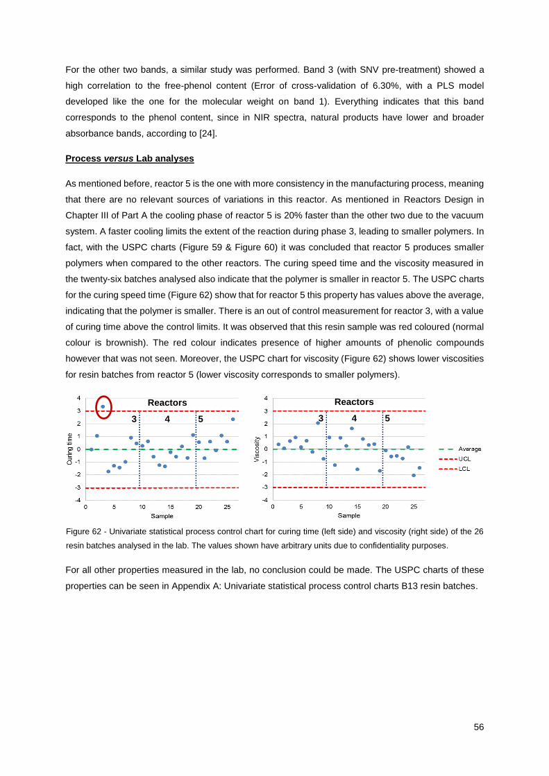
56
For the other two bands, a similar study was performed. Band 3 (with SNV pre-treatment) showed a
high correlation to the free-phenol content (Error of cross-validation of 6.30%, with a PLS model
developed like the one for the molecular weight on band 1). Everything indicates that this band
corresponds to the phenol content, since in NIR spectra, natural products have lower and broader
absorbance bands, according to [24].
Process versus Lab analyses
As mentioned before, reactor 5 is the one with more consistency in the manufacturing process, meaning
that there are no relevant sources of variations in this reactor. As mentioned in Reactors Design in
Chapter III of Part A the cooling phase of reactor 5 is 20% faster than the other two due to the vacuum
system. A faster cooling limits the extent of the reaction during phase 3, leading to smaller polymers. In
fact, with the USPC charts (Figure 59 & Figure 60) it was concluded that reactor 5 produces smaller
polymers when compared to the other reactors. The curing speed time and the viscosity measured in
the twenty-six batches analysed also indicate that the polymer is smaller in reactor 5. The USPC charts
for the curing speed time (Figure 62) show that for reactor 5 this property has values above the average,
indicating that the polymer is smaller. There is an out of control measurement for reactor 3, with a value
of curing time above the control limits. It was observed that this resin sample was red coloured (normal
colour is brownish). The red colour indicates presence of higher amounts of phenolic compounds
however that was not seen. Moreover, the USPC chart for viscosity (Figure 62) shows lower viscosities
for resin batches from reactor 5 (lower viscosity corresponds to smaller polymers).
For all other properties measured in the lab, no conclusion could be made. The USPC charts of these
properties can be seen in Appendix A: Univariate statistical process control charts B13 resin batches.
Reactors
3 4 5
Reactors
3 4 5
Figure 62 - Univariate statistical process control chart for curing time (left side) and viscosity (right side) of the 26
resin batches analysed in the lab. The values shown have arbitrary units due to confidentiality purposes.
57
4. - Conclusions
This Chapter showed that existing historical data contain information that can provide valuable process
knowledge, using MVDA techniques. With multivariate tools to analyse the different types of available
information, a great insight into B13 resin process was achieved. It was also possible to highlight critical
aspects for the final quality of the resin.
Three characteristic bands with the NIR spectral analysis could be identified and linked to each
molecule present in the resin mixture (Band 1: polymer; Band 3: phenol);
Differences were seen between the suppliers in the NIR spectral analysis however it was not
possible to conclude that it is a critical aspect for the resins quality;
Differences between the reactors were seen in both NIR spectral analysis and production
process path. It was possible to conclude that reactor 5 leads to smaller polymers due to the
efficiency of cooling in the third phase;
On the other hand, for reactors 3 and 4, phase 3 was the one with more influence in the quality
of the process. In fact, these two reactors share the cooling system which is a critical aspect for
the resins quality. The cooling system of the reactors should be revised by the company
carefully, especially for reactors 3 and 4. For reactor 5 no critical aspects could be highlighted.
Seasonality effects were not identified for this resin within the studied time frame;
The study of the spectral bands together with the lab analyses performed allowed to conclude
that: Band 1 corresponds to the size of the polymers whereas band 3 corresponds to the amount
of phenol. An alternative quality control for the resins with the implementation of a spectral
library could be done.

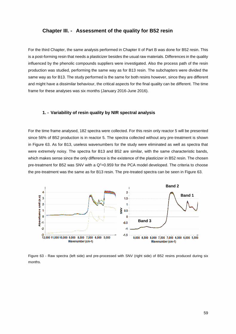
59
Chapter III. - Assessment of the quality for B52 resin
For the third Chapter, the same analysis performed in Chapter II of Part B was done for B52 resin. This
is a post-forming resin that needs a plasticizer besides the usual raw materials. Differences in the quality
influenced by the phenolic compounds suppliers were investigated. Also the process path of the resin
production was studied, performing the same way as for B13 resin. The subchapters were divided the
same way as for B13. The study performed is the same for both resins however, since they are different
and might have a dissimilar behaviour, the critical aspects for the final quality can be different. The time
frame for these analyses was six months (January 2016-June 2016).
1. - Variability of resin quality by NIR spectral analysis
For the time frame analysed, 182 spectra were collected. For this resin only reactor 5 will be presented
since 56% of B52 production is in reactor 5. The spectra collected without any pre-treatment is shown
in Figure 63. As for B13, useless wavenumbers for the study were eliminated as well as spectra that
were extremely noisy. The spectra for B13 and B52 are similar, with the same characteristic bands,
which makes sense since the only difference is the existence of the plasticizer in B52 resin. The chosen
pre-treatment for B52 was SNV with a Q2=0.959 for the PCA model developed. The criteria to choose
the pre-treatment was the same as for B13 resin. The pre-treated spectra can be seen in Figure 63.
Figure 63 - Raw spectra (left side) and pre-processed with SNV (right side) of B52 resins produced during six
months.
Band 1
Band 2
Band 3
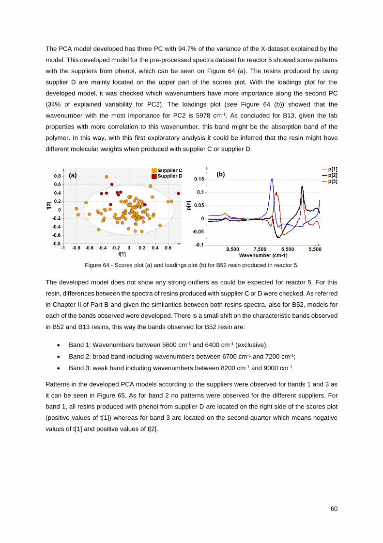
60
The PCA model developed has three PC with 94.7% of the variance of the X-dataset explained by the
model. This developed model for the pre-processed spectra dataset for reactor 5 showed some patterns
with the suppliers from phenol, which can be seen on Figure 64 (a). The resins produced by using
supplier D are mainly located on the upper part of the scores plot. With the loadings plot for the
developed model, it was checked which wavenumbers have more importance along the second PC
(34% of explained variability for PC2). The loadings plot (see Figure 64 (b)) showed that the
wavenumber with the most importance for PC2 is 5978 cm-1. As concluded for B13, given the lab
properties with more correlation to this wavenumber, this band might be the absorption band of the
polymer. In this way, with this first exploratory analysis it could be inferred that the resin might have
different molecular weights when produced with supplier C or supplier D.
The developed model does not show any strong outliers as could be expected for reactor 5. For this
resin, differences between the spectra of resins produced with supplier C or D were checked. As referred
in Chapter II of Part B and given the similarities between both resins spectra, also for B52, models for
each of the bands observed were developed. There is a small shift on the characteristic bands observed
in B52 and B13 resins, this way the bands observed for B52 resin are:
Band 1: Wavenumbers between 5600 cm-1 and 6400 cm-1 (exclusive);
Band 2: broad band including wavenumbers between 6700 cm-1 and 7200 cm-1;
Band 3: weak band including wavenumbers between 8200 cm-1 and 9000 cm-1.
Patterns in the developed PCA models according to the suppliers were observed for bands 1 and 3 as
it can be seen in Figure 65. As for band 2 no patterns were observed for the different suppliers. For
band 1, all resins produced with phenol from supplier D are located on the right side of the scores plot
(positive values of t[1]) whereas for band 3 are located on the second quarter which means negative
values of t[1] and positive values of t[2].
(a) (b)
Figure 64 - Scores plot (a) and loadings plot (b) for B52 resin produced in reactor 5.
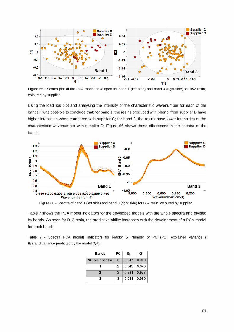
61
Using the loadings plot and analysing the intensity of the characteristic wavenumber for each of the
bands it was possible to conclude that: for band 1, the resins produced with phenol from supplier D have
higher intensities when compared with supplier C; for band 3, the resins have lower intensities of the
characteristic wavenumber with supplier D. Figure 66 shows those differences in the spectra of the
bands.
Table 7 shows the PCA model indicators for the developed models with the whole spectra and divided
by bands. As seen for B13 resin, the predictive ability increases with the development of a PCA model
for each band.
Table 7 - Spectra PCA models indicators for reactor 5: Number of PC (PC), explained variance (
𝑹𝒙𝟐), and variance predicted by the model (Q2).
Figure 66 - Spectra of band 1 (left side) and band 3 (right side) for B52 resin, coloured by supplier.
Band 1 Band 3
Band 1 Band 3
Figure 65 - Scores plot of the PCA model developed for band 1 (left side) and band 3 (right side) for B52 resin,
coloured by supplier.
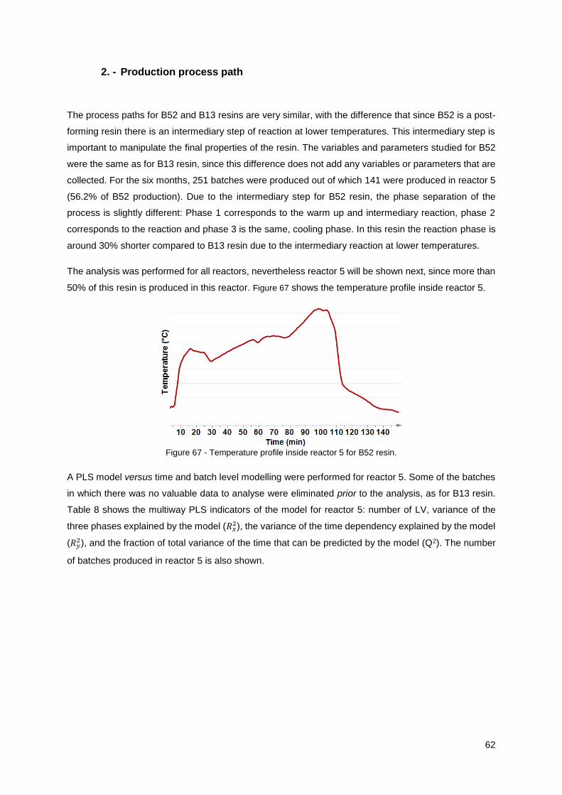
62
2. - Production process path
The process paths for B52 and B13 resins are very similar, with the difference that since B52 is a post-
forming resin there is an intermediary step of reaction at lower temperatures. This intermediary step is
important to manipulate the final properties of the resin. The variables and parameters studied for B52
were the same as for B13 resin, since this difference does not add any variables or parameters that are
collected. For the six months, 251 batches were produced out of which 141 were produced in reactor 5
(56.2% of B52 production). Due to the intermediary step for B52 resin, the phase separation of the
process is slightly different: Phase 1 corresponds to the warm up and intermediary reaction, phase 2
corresponds to the reaction and phase 3 is the same, cooling phase. In this resin the reaction phase is
around 30% shorter compared to B13 resin due to the intermediary reaction at lower temperatures.
The analysis was performed for all reactors, nevertheless reactor 5 will be shown next, since more than
50% of this resin is produced in this reactor. Figure 67 shows the temperature profile inside reactor 5.
Figure 67 - Temperature profile inside reactor 5 for B52 resin.
A PLS model versus time and batch level modelling were performed for reactor 5. Some of the batches
in which there was no valuable data to analyse were eliminated prior to the analysis, as for B13 resin.
Table 8 shows the multiway PLS indicators of the model for reactor 5: number of LV, variance of the
three phases explained by the model (𝑅𝑥2), the variance of the time dependency explained by the model
(𝑅𝑦2), and the fraction of total variance of the time that can be predicted by the model (Q2). The number
of batches produced in reactor 5 is also shown.
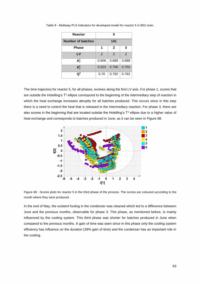
63
Table 8 - Multiway PLS indicators for developed model for reactor 5 in B52 resin.
The time trajectory for reactor 5, for all phases, evolves along the first LV axis. For phase 1, scores that
are outside the Hotelling’s T2 ellipse correspond to the beginning of the intermediary step of reaction in
which the heat exchange increases abruptly for all batches produced. This occurs since in this step
there is a need to control the heat that is released in the intermediary reaction. For phase 3, there are
also scores in the beginning that are located outside the Hotelling’s T2 ellipse due to a higher value of
heat exchange and corresponds to batches produced in June, as it can be seen in Figure 68.
Figure 68 - Scores plots for reactor 5 in the third phase of the process. The scores are coloured according to the
month where they were produced.
In the end of May, the existent fouling in the condenser was cleaned which led to a difference between
June and the previous months, observable for phase 3. This phase, as mentioned before, is mainly
influenced by the cooling system. This third phase was shorter for batches produced in June when
compared to the previous months. A gain of time was seen since in this phase only the cooling system
efficiency has influence on the duration (39% gain of time) and the condenser has an important role in
the cooling.
Reactor 5
Number of batches 141
Phase 1 2 3
LV 2 2 2
𝑹𝒙𝟐 0.606 0.689 0.688
𝑹𝒚𝟐 0.523 0.706 0.703
Q2 0.70 0.792 0.792
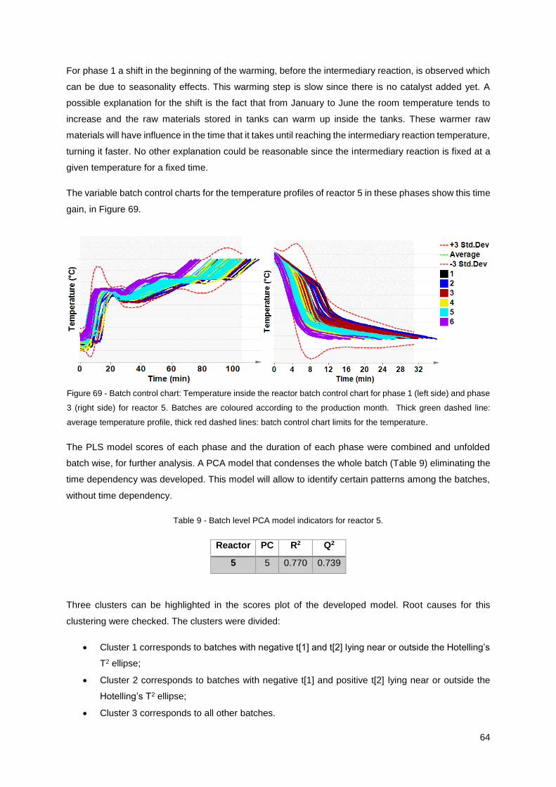
64
For phase 1 a shift in the beginning of the warming, before the intermediary reaction, is observed which
can be due to seasonality effects. This warming step is slow since there is no catalyst added yet. A
possible explanation for the shift is the fact that from January to June the room temperature tends to
increase and the raw materials stored in tanks can warm up inside the tanks. These warmer raw
materials will have influence in the time that it takes until reaching the intermediary reaction temperature,
turning it faster. No other explanation could be reasonable since the intermediary reaction is fixed at a
given temperature for a fixed time.
The variable batch control charts for the temperature profiles of reactor 5 in these phases show this time
gain, in Figure 69.
The PLS model scores of each phase and the duration of each phase were combined and unfolded
batch wise, for further analysis. A PCA model that condenses the whole batch (Table 9) eliminating the
time dependency was developed. This model will allow to identify certain patterns among the batches,
without time dependency.
Table 9 - Batch level PCA model indicators for reactor 5.
Reactor PC R2 Q2
5 5 0.770 0.739
Three clusters can be highlighted in the scores plot of the developed model. Root causes for this
clustering were checked. The clusters were divided:
Cluster 1 corresponds to batches with negative t[1] and t[2] lying near or outside the Hotelling’s
T2 ellipse;
Cluster 2 corresponds to batches with negative t[1] and positive t[2] lying near or outside the
Hotelling’s T2 ellipse;
Cluster 3 corresponds to all other batches.
Figure 69 - Batch control chart: Temperature inside the reactor batch control chart for phase 1 (left side) and phase
3 (right side) for reactor 5. Batches are coloured according to the production month. Thick green dashed line:
average temperature profile, thick red dashed lines: batch control chart limits for the temperature.
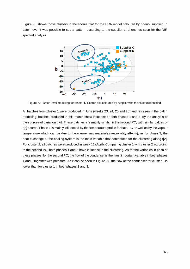
65
Figure 70 shows those clusters in the scores plot for the PCA model coloured by phenol supplier. In
batch level it was possible to see a pattern according to the supplier of phenol as seen for the NIR
spectral analysis.
All batches from cluster 1 were produced in June (weeks 23, 24, 25 and 26) and, as seen in the batch
modelling, batches produced in this month show influence of both phases 1 and 3, by the analysis of
the sources of variation plot. These batches are mainly similar in the second PC, with similar values of
t[2] scores. Phase 1 is mainly influenced by the temperature profile for both PC as well as by the vapour
temperature which can be due to the warmer raw materials (seasonality effects); as for phase 3, the
heat exchange of the cooling system is the main variable that contributes for the clustering along t[2].
For cluster 2, all batches were produced in week 15 (April). Comparing cluster 1 with cluster 2 according
to the second PC, both phases 1 and 3 have influence in the clustering. As for the variables in each of
these phases, for the second PC, the flow of the condenser is the most important variable in both phases
1 and 3 together with pressure. As it can be seen in Figure 71, the flow of the condenser for cluster 2 is
lower than for cluster 1 in both phases 1 and 3.
Figure 70 - Batch level modelling for reactor 5: Scores plot coloured by supplier with the clusters identified.
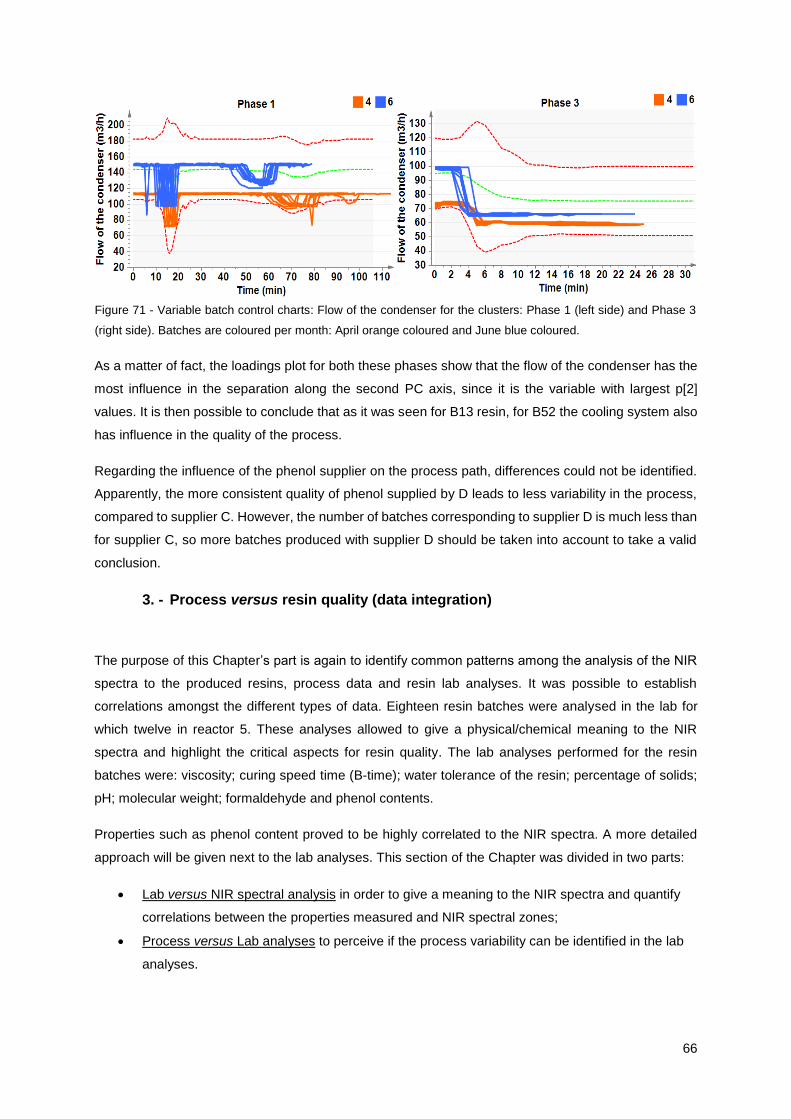
66
As a matter of fact, the loadings plot for both these phases show that the flow of the condenser has the
most influence in the separation along the second PC axis, since it is the variable with largest p[2]
values. It is then possible to conclude that as it was seen for B13 resin, for B52 the cooling system also
has influence in the quality of the process.
Regarding the influence of the phenol supplier on the process path, differences could not be identified.
Apparently, the more consistent quality of phenol supplied by D leads to less variability in the process,
compared to supplier C. However, the number of batches corresponding to supplier D is much less than
for supplier C, so more batches produced with supplier D should be taken into account to take a valid
conclusion.
3. - Process versus resin quality (data integration)
The purpose of this Chapter’s part is again to identify common patterns among the analysis of the NIR
spectra to the produced resins, process data and resin lab analyses. It was possible to establish
correlations amongst the different types of data. Eighteen resin batches were analysed in the lab for
which twelve in reactor 5. These analyses allowed to give a physical/chemical meaning to the NIR
spectra and highlight the critical aspects for resin quality. The lab analyses performed for the resin
batches were: viscosity; curing speed time (B-time); water tolerance of the resin; percentage of solids;
pH; molecular weight; formaldehyde and phenol contents.
Properties such as phenol content proved to be highly correlated to the NIR spectra. A more detailed
approach will be given next to the lab analyses. This section of the Chapter was divided in two parts:
Lab versus NIR spectral analysis in order to give a meaning to the NIR spectra and quantify
correlations between the properties measured and NIR spectral zones;
Process versus Lab analyses to perceive if the process variability can be identified in the lab
analyses.
Figure 71 - Variable batch control charts: Flow of the condenser for the clusters: Phase 1 (left side) and Phase 3
(right side). Batches are coloured per month: April orange coloured and June blue coloured.
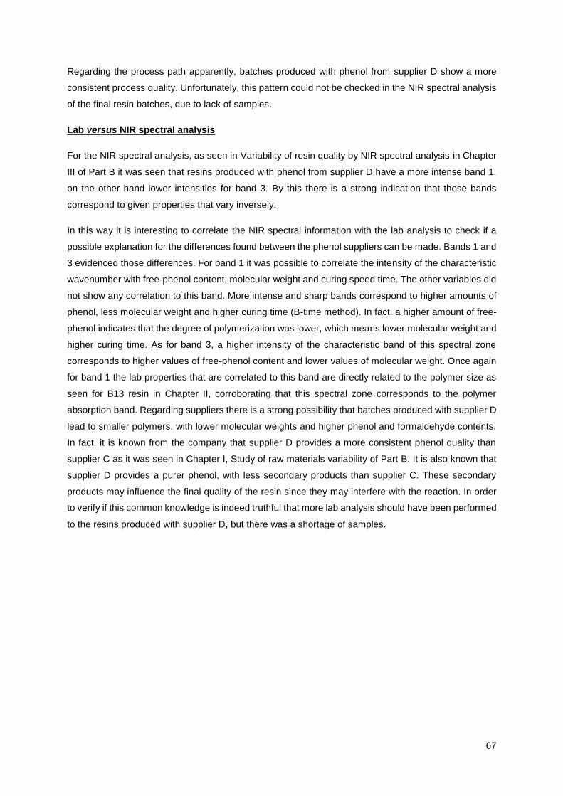
67
Regarding the process path apparently, batches produced with phenol from supplier D show a more
consistent process quality. Unfortunately, this pattern could not be checked in the NIR spectral analysis
of the final resin batches, due to lack of samples.
Lab versus NIR spectral analysis
For the NIR spectral analysis, as seen in Variability of resin quality by NIR spectral analysis in Chapter
III of Part B it was seen that resins produced with phenol from supplier D have a more intense band 1,
on the other hand lower intensities for band 3. By this there is a strong indication that those bands
correspond to given properties that vary inversely.
In this way it is interesting to correlate the NIR spectral information with the lab analysis to check if a
possible explanation for the differences found between the phenol suppliers can be made. Bands 1 and
3 evidenced those differences. For band 1 it was possible to correlate the intensity of the characteristic
wavenumber with free-phenol content, molecular weight and curing speed time. The other variables did
not show any correlation to this band. More intense and sharp bands correspond to higher amounts of
phenol, less molecular weight and higher curing time (B-time method). In fact, a higher amount of free-
phenol indicates that the degree of polymerization was lower, which means lower molecular weight and
higher curing time. As for band 3, a higher intensity of the characteristic band of this spectral zone
corresponds to higher values of free-phenol content and lower values of molecular weight. Once again
for band 1 the lab properties that are correlated to this band are directly related to the polymer size as
seen for B13 resin in Chapter II, corroborating that this spectral zone corresponds to the polymer
absorption band. Regarding suppliers there is a strong possibility that batches produced with supplier D
lead to smaller polymers, with lower molecular weights and higher phenol and formaldehyde contents.
In fact, it is known from the company that supplier D provides a more consistent phenol quality than
supplier C as it was seen in Chapter I, Study of raw materials variability of Part B. It is also known that
supplier D provides a purer phenol, with less secondary products than supplier C. These secondary
products may influence the final quality of the resin since they may interfere with the reaction. In order
to verify if this common knowledge is indeed truthful that more lab analysis should have been performed
to the resins produced with supplier D, but there was a shortage of samples.
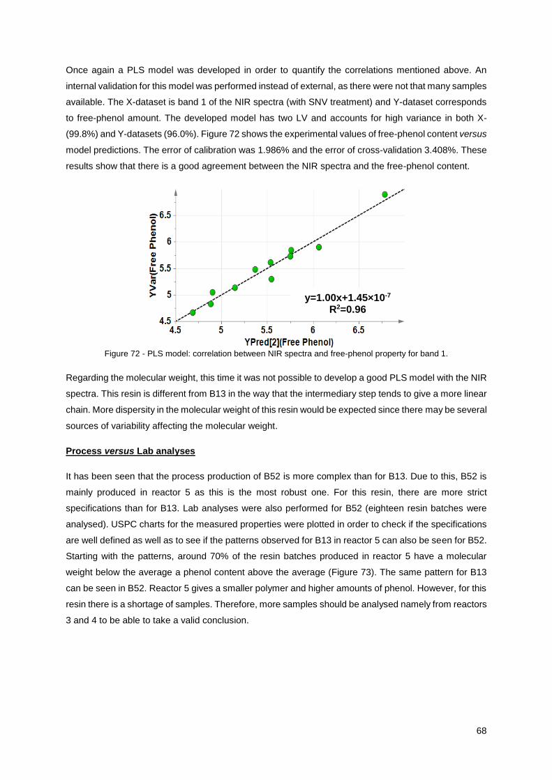
68
Once again a PLS model was developed in order to quantify the correlations mentioned above. An
internal validation for this model was performed instead of external, as there were not that many samples
available. The X-dataset is band 1 of the NIR spectra (with SNV treatment) and Y-dataset corresponds
to free-phenol amount. The developed model has two LV and accounts for high variance in both X-
(99.8%) and Y-datasets (96.0%). Figure 72 shows the experimental values of free-phenol content versus
model predictions. The error of calibration was 1.986% and the error of cross-validation 3.408%. These
results show that there is a good agreement between the NIR spectra and the free-phenol content.
Figure 72 - PLS model: correlation between NIR spectra and free-phenol property for band 1.
Regarding the molecular weight, this time it was not possible to develop a good PLS model with the NIR
spectra. This resin is different from B13 in the way that the intermediary step tends to give a more linear
chain. More dispersity in the molecular weight of this resin would be expected since there may be several
sources of variability affecting the molecular weight.
Process versus Lab analyses
It has been seen that the process production of B52 is more complex than for B13. Due to this, B52 is
mainly produced in reactor 5 as this is the most robust one. For this resin, there are more strict
specifications than for B13. Lab analyses were also performed for B52 (eighteen resin batches were
analysed). USPC charts for the measured properties were plotted in order to check if the specifications
are well defined as well as to see if the patterns observed for B13 in reactor 5 can also be seen for B52.
Starting with the patterns, around 70% of the resin batches produced in reactor 5 have a molecular
weight below the average a phenol content above the average (Figure 73). The same pattern for B13
can be seen in B52. Reactor 5 gives a smaller polymer and higher amounts of phenol. However, for this
resin there is a shortage of samples. Therefore, more samples should be analysed namely from reactors
3 and 4 to be able to take a valid conclusion.
y=1.00x+1.45×10⁻⁷ R2=0.96
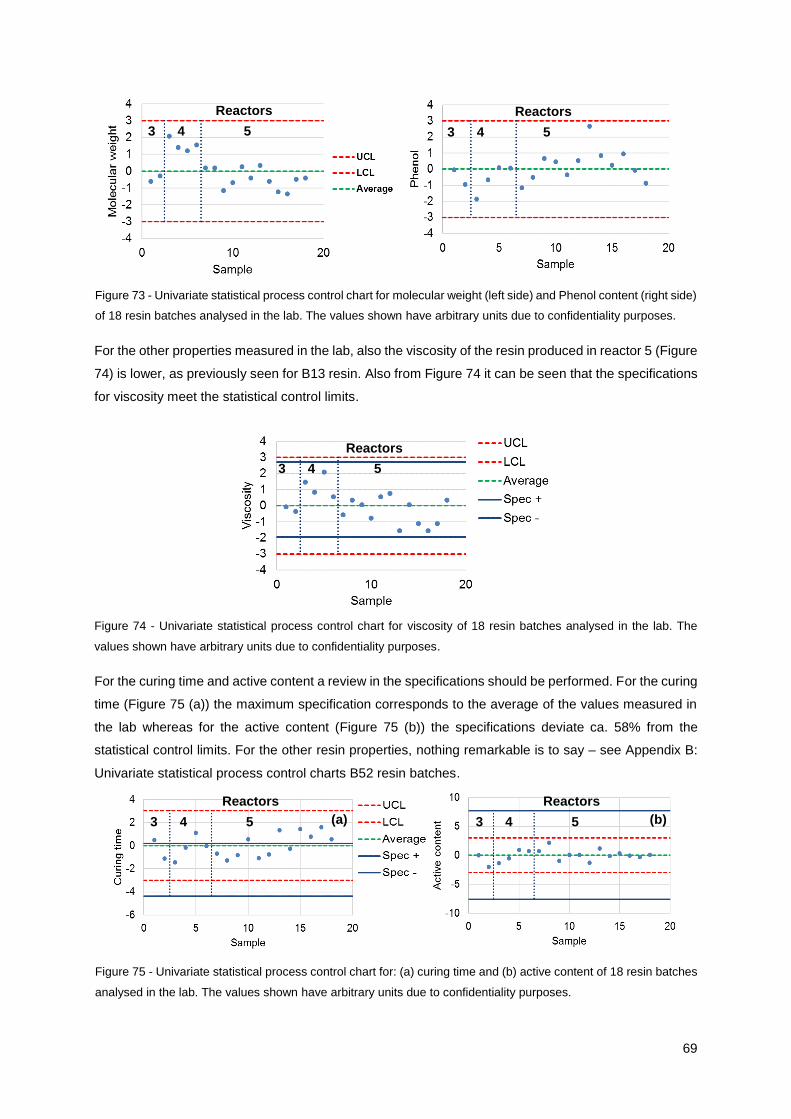
69
For the other properties measured in the lab, also the viscosity of the resin produced in reactor 5 (Figure
74) is lower, as previously seen for B13 resin. Also from Figure 74 it can be seen that the specifications
for viscosity meet the statistical control limits.
Figure 74 - Univariate statistical process control chart for viscosity of 18 resin batches analysed in the lab. The
values shown have arbitrary units due to confidentiality purposes.
For the curing time and active content a review in the specifications should be performed. For the curing
time (Figure 75 (a)) the maximum specification corresponds to the average of the values measured in
the lab whereas for the active content (Figure 75 (b)) the specifications deviate ca. 58% from the
statistical control limits. For the other resin properties, nothing remarkable is to say – see Appendix B:
Univariate statistical process control charts B52 resin batches.
Figure 73 - Univariate statistical process control chart for molecular weight (left side) and Phenol content (right side)
of 18 resin batches analysed in the lab. The values shown have arbitrary units due to confidentiality purposes.
Reactors
3 4 5
Reactors
3 4 5
Reactors
3 4 5
(a) (b)
Figure 75 - Univariate statistical process control chart for: (a) curing time and (b) active content of 18 resin batches
analysed in the lab. The values shown have arbitrary units due to confidentiality purposes.
Reactors
3 4 5
Reactors
3 4 5
70
4. - Conclusions
This Chapter showed that existing historical data contain information that can provide valuable
conclusions, using MVDA techniques. With multivariate tools to analyse the different types of available
information, valuable insight into B52 resin production was achieved. For this resin other critical aspects
for the final resin quality could be highlighted, when compared to B13 resin.
Three characteristic bands with the NIR spectral analysis could be identified and linked to a
specific molecule present in the complex polymeric mixture (Band 3: phenol);
The final quality of the resin depends on the phenol supplier;
It was seen that the flow of the condenser leads to clustering in the process quality. However,
this could not be linked to variability in the resin quality given by NIR.
It was seen that resins produced by phenol from supplier D lead to smaller polymers. This may
be due to the existence of secondary products in phenol from supplier C that are not present in
supplier D (differences already observed in the study of the raw materials variability);
An alternative quality control for the resins with the implementation of a spectral library could be
done with the quantified correlation between the phenol content analysis and the NIR spectra.
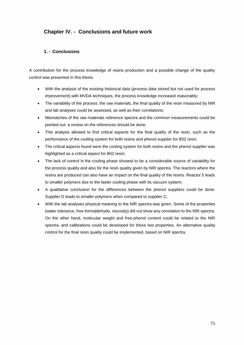
71
Chapter IV. - Conclusions and future work
1. - Conclusions
A contribution for the process knowledge of resins production and a possible change of the quality
control was presented in this thesis.
With the analysis of the existing historical data (process data stored but not used for process
improvement) with MVDA techniques, the process knowledge increased reasonably;
The variability of the process, the raw materials, the final quality of the resin measured by NIR
and lab analyses could be assessed, as well as their correlations;
Mismatches of the raw materials reference spectra and the common measurements could be
pointed out: a review on the references should be done;
This analysis allowed to find critical aspects for the final quality of the resin, such as the
performance of the cooling system for both resins and phenol supplier for B52 resin.
The critical aspects found were the cooling system for both resins and the phenol supplier was
highlighted as a critical aspect for B52 resin;
The lack of control in the cooling phase showed to be a considerable source of variability for
the process quality and also for the resin quality given by NIR spectra. The reactors where the
resins are produced can also have an impact on the final quality of the resins. Reactor 5 leads
to smaller polymers due to the faster cooling phase with its vacuum system;
A qualitative conclusion for the differences between the phenol suppliers could be done:
Supplier D leads to smaller polymers when compared to supplier C;
With the lab analyses physical meaning to the NIR spectra was given. Some of the properties
(water tolerance, free-formaldehyde, viscosity) did not show any correlation to the NIR spectra.
On the other hand, molecular weight and free-phenol content could be related to the NIR
spectra, and calibrations could be developed for these two properties. An alternative quality
control for the final resin quality could be implemented, based on NIR spectra.
72
2. - Future Work
For B52 resin there was a shortage of samples, namely resin batches produced with phenol
from supplier D. More than 80% of the resin batches were produced with supplier C, within the
studied time frame. The performed study should be extended for a longer period, in order to
validate the presented conclusions;
The developed calibrations for phenol content and molecular weight should be improved if they
are to be used as a new quality control tool;
The PCA models based on the resin NIR spectra together with the lab analyses showed that a
quality control based on an NIR spectral library should be possible, replacing the current
method. Further development and validation of these spectral libraries is advised.
73
References
[1] Trespa International B.V., [Online]. Available: http://www.trespa.com. [Accessed 14 April 2016].
[2] Trespa International BV, “Beschrijving reactoren,” 2016.
[3] A. P. L. Gardziella, in Phenolic Resins, 2nd ed., Berlin, New York, Barcelona, Hong Kong,
London, Milan, Paris, Singapore, Tokyo, Springer, 2000, pp. 24-82.
[4] Y. Salubi, “Monitoring of fire retardant grade resins with respect to NIR quality control”.
[5] M. Otto, Chemometrics, Weinheim: Wiley-VCH, 1999.
[6] R. G. Brereton, Chemometrics: Data Analysis for the Laboratory and Chemical Plant, Chichester:
John Wiley & Sons Ltd., 2003, pp. 1-12.
[7] X. Z. Wang, “Data Mining and Knowledge Discovery for Process Monitoring and Control,” in
Advances in Industrial Control, London, Springer-Verlag, 1999, pp. 29-59.
[8] T. Næs, T. Isaksson, T. Fearn and T. Davies, A User-Friendly Guide to Multivariate Calibration
and Classification, Chichester: NIR Publications, 2002.
[9] L. Eriksson, E.Johansson, N.Kettaneh-Wold, J. Tryg, C.Wikström and a. S.Wold, “Multi- and
Megavariate Data Analysis,” in Part I - Basic and Principles Applications, Umea, Umetrics AB,
2006.
[10] D. T. Dearing, “Centre for Process Analysis & Control,” 2012. [Online]. Available:
http://depts.washington.edu/cpac/Activities/Meetings/documents/DearingFundamentalsofChem
ometrics.pdf. [Accessed July 2016].
[11] V. M. d. C. L. Lourenço, A Quality by design study of an Industrial Fluid Bed Granulation Process,
Lisboa, 2011.
[12] S. Wold, M. Sjöström and L. Eriksson, “PLS-regression: a basic tool of chemometrics”. Sweden
2001.
[13] H. W. Siesler, “Basic Principles of Near-Infrared Spectroscopy,” in Handbook of Near-Infrared
Analysis, Boca Raton, CRC Press , 2008, pp. 7-18.
[14] PerkinElmer Inc., 2016. [Online]. Available: http://www.perkinelmer.com/category/infrared-ir-
instruments. [Accessed August 2016].
74
[15] Bruker, Bruker, 2016. [Online]. Available: https://www.bruker.com/products/infrared-near-
infrared-and-raman-spectroscopy/ft-nir/mpa/overview.html. [Accessed August 2016].
[16] A. Holmes, “Combination Bands, Overtones and Fermi Resonances,” Chemistry LibreTexts,
September 2016. [Online]. Available:
http://chem.libretexts.org/Core/Physical_and_Theoretical_Chemistry/Spectroscopy/Vibrational_
Spectroscopy/Vibrational_Modes/Combination_Bands%2C_Overtones_and_Fermi_Resonanc
es. [Accessed August 2016].
[17] B. C. Smith, “Introduction to Infrared Spectroscopy,” in Fundamentals of Fourier Transfom
Infrared Spectroscopy, Boca Raton, CRC Press, 2011, pp. 1-17.
[18] K. Helwegen, Development of a fire retardant resin, Weert: Trespa International BV, 2010.
[19] Deutsche Norm, DIN EN ISO 11402 - Phenolic, amino and condensation resins, September
2005.
[20] J. Clark, “The Fingerprint Region,” Chemistry LibreTexts, December 2013. [Online]. Available:
http://chem.libretexts.org/Core/Physical_Chemistry/Spectroscopy/Vibrational_Spectroscopy/Infr
ared_Spectroscopy/The_Fingerprint_Region. [Accessed August 2016].
[21] J. Huang, S. Romero-Torres and M. Moshgbar, “Practical Considerations in Data Pre-treatment
for NIR and Raman Spectroscopy,” 1 October 2010.
[22] “Department of Chemistry,” Michigan State University, 5 May 2013. [Online]. Available:
https://www2.chemistry.msu.edu/faculty/reusch/virttxtjml/Spectrpy/InfraRed/infrared.htm.
[Accessed April 2016].
[23] M. S. Dhanoa, S. Lister, R. Sanderson and R. Barnes, “The Link between Multiplicative Scatter
Correction (MSC) and Standard Normal Variate (SNV) Transformations of NIR spectra,” Journal
of Near Infrared Spectroscopy, vol. Volume 2, no. Issue 1, pp. 43-47, 1994.
[24] C. K. Lee and K. A., “NIR Analysis of Polymers,” in Handbook of Near-Infrared Analysis, Boca
Raton, CRC Press, 2008, pp. 530-563.
[25] O. Ivanov, Applications and Experiences of Quality Control, Rijeka: InTech, 2011.
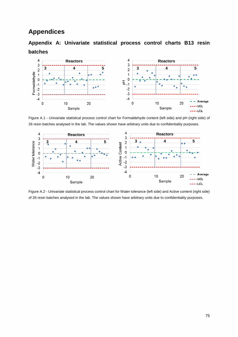
75
Appendices
Appendix A: Univariate statistical process control charts B13 resin
batches
Reactors
3 4 5
Reactors
3 4 5
Figure A.1 - Univariate statistical process control chart for Formaldehyde content (left side) and pH (right side) of
26 resin batches analysed in the lab. The values shown have arbitrary units due to confidentiality purposes.
Reactors
3 4 5
Reactors
3 4 5
Figure A.2 - Univariate statistical process control chart for Water tolerance (left side) and Active content (right side)
of 26 resin batches analysed in the lab. The values shown have arbitrary units due to confidentiality purposes.
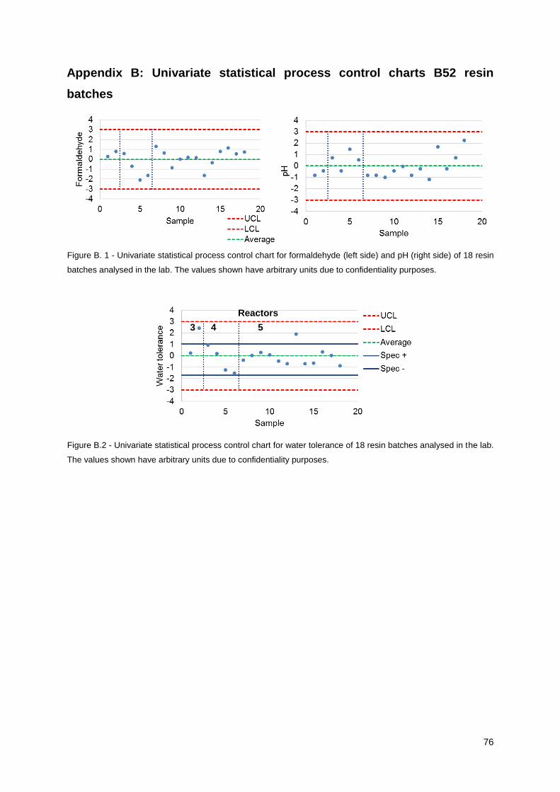
76
Appendix B: Univariate statistical process control charts B52 resin
batches
Reactors
3 4 5
Reactors
3 4 5
Figure B. 1 - Univariate statistical process control chart for formaldehyde (left side) and pH (right side) of 18 resin
batches analysed in the lab. The values shown have arbitrary units due to confidentiality purposes.
Reactors
3 4 5
Figure B.2 - Univariate statistical process control chart for water tolerance of 18 resin batches analysed in the lab.
The values shown have arbitrary units due to confidentiality purposes.