advanced algebra for teacherszimmer.csufresno.edu/~lburger/math 139 (1_3).pdf · advanced algebra...
TRANSCRIPT

Advanced Algebra for Teachers (Revised Edition)
By Kirthi Premadasa, Rajee Amarasinghe, and Oscar Vega
California State University, Fresno

Bassim Hamadeh, CEO and PublisherChristopher Foster, General Vice PresidentMichael Simpson, Vice President of AcquisitionsJessica Knott, Managing EditorKevin Fahey, Cognella Marketing ManagerJess Busch, Senior Graphic Designer
Copyright © 2013 by Cognella, Inc. All rights reserved. No part of this publication may be reprinted, reproduced, transmitted, or utilized in any form or by any electronic, mechanical, or other means, now known or hereafter invented, including photocopying, microfilming, and recording, or in any information retrieval system without the written permission of Cognella, Inc.
First published in the United States of America in 2013 by Cognella, Inc.
Trademark Notice: Product or corporate names may be trademarks or registered trademarks, and are used only for identification and explanation without intent to infringe.
Printed in the United States of America
ISBN: 978-1-93555-157-7 (pbk)

Contents
1 Expressions and Equations . . . . . . . . . . . . . . . . . . . . . . . . . . . . . . . . . . . . . . . . . . . . . . . . . . . . . . . . . . . . . 11.1 Introduction . . . . . . . . . . . . . . . . . . . . . . . . . . . . . . . . . . . . . . . . . . . . . . . . . . . . . . . . . . . . . . . . . . . . . . 11.2 Number Systems . . . . . . . . . . . . . . . . . . . . . . . . . . . . . . . . . . . . . . . . . . . . . . . . . . . . . . . . . . . . . . . . . . 1
1.2.1 Types of Numbers and Notation . . . . . . . . . . . . . . . . . . . . . . . . . . . . . . . . . . . . . . . . . . . . . . . 11.2.2 How Various Numbers are Related to Each Other . . . . . . . . . . . . . . . . . . . . . . . . . . . . . . . . 2
1.3 Algebraic Expressions . . . . . . . . . . . . . . . . . . . . . . . . . . . . . . . . . . . . . . . . . . . . . . . . . . . . . . . . . . . . . 21.4 Equations . . . . . . . . . . . . . . . . . . . . . . . . . . . . . . . . . . . . . . . . . . . . . . . . . . . . . . . . . . . . . . . . . . . . . . . . 4
1.4.1 Solving Linear Equations . . . . . . . . . . . . . . . . . . . . . . . . . . . . . . . . . . . . . . . . . . . . . . . . . . . . 41.5 Solving a System of Equations . . . . . . . . . . . . . . . . . . . . . . . . . . . . . . . . . . . . . . . . . . . . . . . . . . . . . . 5
1.5.1 Solving a System by Graphing . . . . . . . . . . . . . . . . . . . . . . . . . . . . . . . . . . . . . . . . . . . . . . . . 51.6 Solving Linear Inequalities . . . . . . . . . . . . . . . . . . . . . . . . . . . . . . . . . . . . . . . . . . . . . . . . . . . . . . . . . 71.7 The Graph of a Single Linear Inequality . . . . . . . . . . . . . . . . . . . . . . . . . . . . . . . . . . . . . . . . . . . . . . . 71.8 Graphing a System of Two or More Inequalities . . . . . . . . . . . . . . . . . . . . . . . . . . . . . . . . . . . . . . . . 11
2 Quadratic Equations . . . . . . . . . . . . . . . . . . . . . . . . . . . . . . . . . . . . . . . . . . . . . . . . . . . . . . . . . . . . . . . . . . 232.1 The Quadratic Formula . . . . . . . . . . . . . . . . . . . . . . . . . . . . . . . . . . . . . . . . . . . . . . . . . . . . . . . . . . . . . 232.2 Rational Equations That Lead to Quadratic Equations . . . . . . . . . . . . . . . . . . . . . . . . . . . . . . . . . . . 242.3 Quadratic Equations With Complex Coefficients . . . . . . . . . . . . . . . . . . . . . . . . . . . . . . . . . . . . . . . 252.4 Equations That Transform Into Quadratic Equations . . . . . . . . . . . . . . . . . . . . . . . . . . . . . . . . . . . . 272.5 Manipulation of Roots of Quadratic Equations . . . . . . . . . . . . . . . . . . . . . . . . . . . . . . . . . . . . . . . . . 282.6 Solving Quadratic Equations by Completing the Square. . . . . . . . . . . . . . . . . . . . . . . . . . . . . . . . . . 28
3 Relations and Functions . . . . . . . . . . . . . . . . . . . . . . . . . . . . . . . . . . . . . . . . . . . . . . . . . . . . . . . . . . . . . . . 333.1 Relations . . . . . . . . . . . . . . . . . . . . . . . . . . . . . . . . . . . . . . . . . . . . . . . . . . . . . . . . . . . . . . . . . . . . . . . . 33
3.1.1 Domain and Range of a Relation . . . . . . . . . . . . . . . . . . . . . . . . . . . . . . . . . . . . . . . . . . . . . . 333.2 What is a Function? . . . . . . . . . . . . . . . . . . . . . . . . . . . . . . . . . . . . . . . . . . . . . . . . . . . . . . . . . . . . . . . . 363.3 The Domain of a Function . . . . . . . . . . . . . . . . . . . . . . . . . . . . . . . . . . . . . . . . . . . . . . . . . . . . . . . . . . 373.4 The Graph of a Function . . . . . . . . . . . . . . . . . . . . . . . . . . . . . . . . . . . . . . . . . . . . . . . . . . . . . . . . . . . . 38
3.4.1 The Vertical Line Test. . . . . . . . . . . . . . . . . . . . . . . . . . . . . . . . . . . . . . . . . . . . . . . . . . . . . . . . 393.5 Algebra of Functions . . . . . . . . . . . . . . . . . . . . . . . . . . . . . . . . . . . . . . . . . . . . . . . . . . . . . . . . . . . . . . . 393.6 One-to-one Functions . . . . . . . . . . . . . . . . . . . . . . . . . . . . . . . . . . . . . . . . . . . . . . . . . . . . . . . . . . . . . . 40
3.6.1 The Horizontal Line Test. . . . . . . . . . . . . . . . . . . . . . . . . . . . . . . . . . . . . . . . . . . . . . . . . . . . . 413.7 The Inverse of a Function . . . . . . . . . . . . . . . . . . . . . . . . . . . . . . . . . . . . . . . . . . . . . . . . . . . . . . . . . . . 423.8 The Graph of the Inverse Function . . . . . . . . . . . . . . . . . . . . . . . . . . . . . . . . . . . . . . . . . . . . . . . . . . . 423.9 How to Find the Inverse Function? . . . . . . . . . . . . . . . . . . . . . . . . . . . . . . . . . . . . . . . . . . . . . . . . . . . 43
vii

viii Contents
4 Polynomials . . . . . . . . . . . . . . . . . . . . . . . . . . . . . . . . . . . . . . . . . . . . . . . . . . . . . . . . . . . . . . . . . . . . . . . . . . 474.1 Finding Roots of Polynomials . . . . . . . . . . . . . . . . . . . . . . . . . . . . . . . . . . . . . . . . . . . . . . . . . . . . . . . 474.2 Conjugate Root Theorems . . . . . . . . . . . . . . . . . . . . . . . . . . . . . . . . . . . . . . . . . . . . . . . . . . . . . . . . . . 504.3 Graphs of Polynomials . . . . . . . . . . . . . . . . . . . . . . . . . . . . . . . . . . . . . . . . . . . . . . . . . . . . . . . . . . . . . 514.4 The Sum and Product of the Roots of a Polynomial . . . . . . . . . . . . . . . . . . . . . . . . . . . . . . . . . . . . . 584.5 Rational Functions . . . . . . . . . . . . . . . . . . . . . . . . . . . . . . . . . . . . . . . . . . . . . . . . . . . . . . . . . . . . . . . . 59
5 The Binomial Theorem . . . . . . . . . . . . . . . . . . . . . . . . . . . . . . . . . . . . . . . . . . . . . . . . . . . . . . . . . . . . . . . . 715.1 What is the Binomial Theorem? . . . . . . . . . . . . . . . . . . . . . . . . . . . . . . . . . . . . . . . . . . . . . . . . . . . . . 715.2 Binomial Expansions Using Pascal’s Triangle . . . . . . . . . . . . . . . . . . . . . . . . . . . . . . . . . . . . . . . . . . 735.3 Working With Specific Terms of a Binomial Expansion . . . . . . . . . . . . . . . . . . . . . . . . . . . . . . . . . . 73
6 Radicals . . . . . . . . . . . . . . . . . . . . . . . . . . . . . . . . . . . . . . . . . . . . . . . . . . . . . . . . . . . . . . . . . . . . . . . . . . . . . 776.1 Simplifying Radicals . . . . . . . . . . . . . . . . . . . . . . . . . . . . . . . . . . . . . . . . . . . . . . . . . . . . . . . . . . . . . . . 776.2 Radical Equations . . . . . . . . . . . . . . . . . . . . . . . . . . . . . . . . . . . . . . . . . . . . . . . . . . . . . . . . . . . . . . . . . 79
6.2.1 Single Radical Equations . . . . . . . . . . . . . . . . . . . . . . . . . . . . . . . . . . . . . . . . . . . . . . . . . . . . . 796.2.2 Double Radical Equations . . . . . . . . . . . . . . . . . . . . . . . . . . . . . . . . . . . . . . . . . . . . . . . . . . . . 80
6.3 Graphs of Radical Functions . . . . . . . . . . . . . . . . . . . . . . . . . . . . . . . . . . . . . . . . . . . . . . . . . . . . . . . . 816.3.1 Graphing Radical Functions With Even Index . . . . . . . . . . . . . . . . . . . . . . . . . . . . . . . . . . . 816.3.2 Graphing Radical Functions With Odd Index . . . . . . . . . . . . . . . . . . . . . . . . . . . . . . . . . . . . 84
7 Exponential and Logarithmic Functions . . . . . . . . . . . . . . . . . . . . . . . . . . . . . . . . . . . . . . . . . . . . . . . . . 877.1 Exponential Functions . . . . . . . . . . . . . . . . . . . . . . . . . . . . . . . . . . . . . . . . . . . . . . . . . . . . . . . . . . . . . 87
7.1.1 The Graph of f (x) = ax, for a > 1 . . . . . . . . . . . . . . . . . . . . . . . . . . . . . . . . . . . . . . . . . . . . . 877.1.2 The Graph of f (x) = ax, for a < 1 . . . . . . . . . . . . . . . . . . . . . . . . . . . . . . . . . . . . . . . . . . . . . 89
7.2 Other Problems Involving Exponential Functions . . . . . . . . . . . . . . . . . . . . . . . . . . . . . . . . . . . . . . . 917.3 The Natural Exponential Function . . . . . . . . . . . . . . . . . . . . . . . . . . . . . . . . . . . . . . . . . . . . . . . . . . . . 927.4 Logarithmic Functions . . . . . . . . . . . . . . . . . . . . . . . . . . . . . . . . . . . . . . . . . . . . . . . . . . . . . . . . . . . . . 947.5 Properties of Logarithms . . . . . . . . . . . . . . . . . . . . . . . . . . . . . . . . . . . . . . . . . . . . . . . . . . . . . . . . . . . 977.6 Exponential Equations . . . . . . . . . . . . . . . . . . . . . . . . . . . . . . . . . . . . . . . . . . . . . . . . . . . . . . . . . . . . . 997.7 Logarithmic Equations . . . . . . . . . . . . . . . . . . . . . . . . . . . . . . . . . . . . . . . . . . . . . . . . . . . . . . . . . . . . . 101
8 Linear Algebra . . . . . . . . . . . . . . . . . . . . . . . . . . . . . . . . . . . . . . . . . . . . . . . . . . . . . . . . . . . . . . . . . . . . . . . 1078.1 Matrices . . . . . . . . . . . . . . . . . . . . . . . . . . . . . . . . . . . . . . . . . . . . . . . . . . . . . . . . . . . . . . . . . . . . . . . . . 1078.2 Matrix Operations . . . . . . . . . . . . . . . . . . . . . . . . . . . . . . . . . . . . . . . . . . . . . . . . . . . . . . . . . . . . . . . . . 107
8.2.1 Matrix Addition . . . . . . . . . . . . . . . . . . . . . . . . . . . . . . . . . . . . . . . . . . . . . . . . . . . . . . . . . . . . 1078.2.2 Matrix Multiplication . . . . . . . . . . . . . . . . . . . . . . . . . . . . . . . . . . . . . . . . . . . . . . . . . . . . . . . . 1088.2.3 Scalar Multiplication . . . . . . . . . . . . . . . . . . . . . . . . . . . . . . . . . . . . . . . . . . . . . . . . . . . . . . . . 109
8.3 Special Types of Matrices. . . . . . . . . . . . . . . . . . . . . . . . . . . . . . . . . . . . . . . . . . . . . . . . . . . . . . . . . . . 1108.3.1 Diagonal Matrices . . . . . . . . . . . . . . . . . . . . . . . . . . . . . . . . . . . . . . . . . . . . . . . . . . . . . . . . . . 1108.3.2 Symmetric Matrices . . . . . . . . . . . . . . . . . . . . . . . . . . . . . . . . . . . . . . . . . . . . . . . . . . . . . . . . . 1108.3.3 Upper Triangular Matrices . . . . . . . . . . . . . . . . . . . . . . . . . . . . . . . . . . . . . . . . . . . . . . . . . . . 1118.3.4 Lower Triangular Matrices . . . . . . . . . . . . . . . . . . . . . . . . . . . . . . . . . . . . . . . . . . . . . . . . . . . 111
8.4 Linear Systems of Equations and Row Operations. . . . . . . . . . . . . . . . . . . . . . . . . . . . . . . . . . . . . . . 1118.4.1 Row Operations . . . . . . . . . . . . . . . . . . . . . . . . . . . . . . . . . . . . . . . . . . . . . . . . . . . . . . . . . . . . 1128.4.2 Row Echelon Form . . . . . . . . . . . . . . . . . . . . . . . . . . . . . . . . . . . . . . . . . . . . . . . . . . . . . . . . . . 1148.4.3 Solving Systems of Linear Equations Using Row Operations . . . . . . . . . . . . . . . . . . . . . . . 116
8.5 Determinants . . . . . . . . . . . . . . . . . . . . . . . . . . . . . . . . . . . . . . . . . . . . . . . . . . . . . . . . . . . . . . . . . . . . . 1218.6 Properties of Determinants . . . . . . . . . . . . . . . . . . . . . . . . . . . . . . . . . . . . . . . . . . . . . . . . . . . . . . . . . . 1228.7 Solving Systems of Equations Suing Cramer’s Rule . . . . . . . . . . . . . . . . . . . . . . . . . . . . . . . . . . . . . 1258.8 The Inverse of a Matrix . . . . . . . . . . . . . . . . . . . . . . . . . . . . . . . . . . . . . . . . . . . . . . . . . . . . . . . . . . . . . 126
8.8.1 How to Find the Inverse of a Matrix . . . . . . . . . . . . . . . . . . . . . . . . . . . . . . . . . . . . . . . . . . . . 126

Contents ix
8.9 Vectors . . . . . . . . . . . . . . . . . . . . . . . . . . . . . . . . . . . . . . . . . . . . . . . . . . . . . . . . . . . . . . . . . . . . . . . . . . 1278.9.1 Vector Algebra . . . . . . . . . . . . . . . . . . . . . . . . . . . . . . . . . . . . . . . . . . . . . . . . . . . . . . . . . . . . . 1288.9.2 The Dot Product . . . . . . . . . . . . . . . . . . . . . . . . . . . . . . . . . . . . . . . . . . . . . . . . . . . . . . . . . . . . 131
8.10 Vectors in a Three-Dimensional Space . . . . . . . . . . . . . . . . . . . . . . . . . . . . . . . . . . . . . . . . . . . . . . . . 1328.10.1 The Cross Product . . . . . . . . . . . . . . . . . . . . . . . . . . . . . . . . . . . . . . . . . . . . . . . . . . . . . . . . . . 132
9 Number Theory . . . . . . . . . . . . . . . . . . . . . . . . . . . . . . . . . . . . . . . . . . . . . . . . . . . . . . . . . . . . . . . . . . . . . . . 1419.1 Division . . . . . . . . . . . . . . . . . . . . . . . . . . . . . . . . . . . . . . . . . . . . . . . . . . . . . . . . . . . . . . . . . . . . . . . . . 1419.2 Prime Numbers. . . . . . . . . . . . . . . . . . . . . . . . . . . . . . . . . . . . . . . . . . . . . . . . . . . . . . . . . . . . . . . . . . . . 1419.3 The Fundamental Theorem of Arithmetic. . . . . . . . . . . . . . . . . . . . . . . . . . . . . . . . . . . . . . . . . . . . . . 1449.4 The greatest Common Divisor . . . . . . . . . . . . . . . . . . . . . . . . . . . . . . . . . . . . . . . . . . . . . . . . . . . . . . . 1469.5 The Least Common Multiple . . . . . . . . . . . . . . . . . . . . . . . . . . . . . . . . . . . . . . . . . . . . . . . . . . . . . . . . 1479.6 The Euclidean Algorithm. . . . . . . . . . . . . . . . . . . . . . . . . . . . . . . . . . . . . . . . . . . . . . . . . . . . . . . . . . . 1499.7 Mathematical Induction. . . . . . . . . . . . . . . . . . . . . . . . . . . . . . . . . . . . . . . . . . . . . . . . . . . . . . . . . . . . . 1509.8 Divisibility Tests. . . . . . . . . . . . . . . . . . . . . . . . . . . . . . . . . . . . . . . . . . . . . . . . . . . . . . . . . . . . . . . . . . . 1549.9 A Few Important Theorems. . . . . . . . . . . . . . . . . . . . . . . . . . . . . . . . . . . . . . . . . . . . . . . . . . . . . . . . . 155
10 Abstract Algebra . . . . . . . . . . . . . . . . . . . . . . . . . . . . . . . . . . . . . . . . . . . . . . . . . . . . . . . . . . . . . . . . . . . . . . 15910.1 Introduction . . . . . . . . . . . . . . . . . . . . . . . . . . . . . . . . . . . . . . . . . . . . . . . . . . . . . . . . . . . . . . . . . . . . . . 15910.2 Closure Property . . . . . . . . . . . . . . . . . . . . . . . . . . . . . . . . . . . . . . . . . . . . . . . . . . . . . . . . . . . . . . . . . . 15910.3 The Associative Property . . . . . . . . . . . . . . . . . . . . . . . . . . . . . . . . . . . . . . . . . . . . . . . . . . . . . . . . . . . 16110.4 The Commutative Property . . . . . . . . . . . . . . . . . . . . . . . . . . . . . . . . . . . . . . . . . . . . . . . . . . . . . . . . . 16110.5 The Existence of an Identity . . . . . . . . . . . . . . . . . . . . . . . . . . . . . . . . . . . . . . . . . . . . . . . . . . . . . . . . . 16210.6 The Existence of Inverses . . . . . . . . . . . . . . . . . . . . . . . . . . . . . . . . . . . . . . . . . . . . . . . . . . . . . . . . . . . 16410.7 Groups . . . . . . . . . . . . . . . . . . . . . . . . . . . . . . . . . . . . . . . . . . . . . . . . . . . . . . . . . . . . . . . . . . . . . . . . . . 16510.8 Rings and Fields . . . . . . . . . . . . . . . . . . . . . . . . . . . . . . . . . . . . . . . . . . . . . . . . . . . . . . . . . . . . . . . . . . 16610.9 Fields . . . . . . . . . . . . . . . . . . . . . . . . . . . . . . . . . . . . . . . . . . . . . . . . . . . . . . . . . . . . . . . . . . . . . . . . . . . 17010.10 Ordered Fields . . . . . . . . . . . . . . . . . . . . . . . . . . . . . . . . . . . . . . . . . . . . . . . . . . . . . . . . . . . . . . . . . . . 174
Index . . . . . . . . . . . . . . . . . . . . . . . . . . . . . . . . . . . . . . . . . . . . . . . . . . . . . . . . . . . . . . . . . . . . . . . . . . . . . . . . . . . . 179

Preface
The purpose of this text is to provide a much needed resource for secondary school math teachers who arestriving to acquire the knowledge for state certification in algebra. Today, most secondary school math teachersare required to have a knowledge of algebra that covers the full range of algebraic topics there are; startingfrom high school algebra all the way to the level of abstract algebra learned by senior math majors.
One of the main bottlenecks standing in the way of a secondary school teacher trying to acquire this knowl-edge is the lack of a single text which covers this variety of topics in a practical and user-friendly manner.This book is aimed at satisfying that requirement. On the one hand, a typical college algebra text falls short ofmeeting the required standard, both in the range of the content and the depth of the material, while on the otherhand a typical abstract algebra textbook , which covers the deeper material, falls short of covering the basic andintermediate material. This book will cover the most relevant topics in the undergraduate algebra spectrum tothe range and depth optimal to a typical certification examination.
Even though the chapters of this book are in close alignment with the subject matter relevance sections of theCalifornia certification examination for Algebra and Number Theory (CSET subtest for Algebra and NumberTheory), the topics should also cover similar requirements in most other states.
The text is written with the practical teacher in mind. The book exposes the reader to the concepts andthe techniques of the different topics in a gradual manner through a series of worked out examples, whichrange from the simplest of exercises to the harder problems. This method, which deviates from the traditionaltheorem-proof approach should benefit a teacher that is hoping to acquire the expertise in a limited time frame.Each chapter is followed by a good collection of problems of all levels which the reader is encouraged toattempt in order to reinforce the required problem solving skills.
The author team has used their experience teaching abstract algebra and number theory topics to non-mathmajors to bring across the abstract concepts in a simple manner. The essence of abstract algebra is presentedusing classification attempts found in other sciences as a motivation, and the reader is motivated to discoverand understand the meaning of concepts such as identity and inverse using diagrams that are easy to visualize.
Covering a full range of algebra topics in a single text in a user friendly manner is by no means an easy task.However, the authors are confident that this book will fill the need of the hour for secondary school teacherswho are planning to enhance their knowledge base in algebra and number theory. The confidence that authorshave is reinforced by the fact that the material of this book has been used at several workshops for Californiateachers who were planning to take the Algebra and Number Theory subtest, which resulted in an exceptionallyhigh passing rate.
The AuthorsJuly, 2012
xi
Chapter 1Expressions and Equations
Abstract In this section we will introduce you to the very foundations of algebra. We will start by showinghow the natural numbers initiate the evolution of the number systems, which stretches all the way to complexnumbers and will go on to show how these number systems are linked to one another. We will then presentsome of the basic algebraic expressions that you would encounter throughout this book and their geometricrationale. We will then, gently, introduce the art of solving equations by presenting the simplest scenario whichinvolves the solving of single and multiple linear equations and inequalities using different approaches.
1.1 Introduction
In school’s mathematics curricula, Algebra has gone through major changes in the past few years. The pointat which students should learn algebra and how they should learn it has been debated throughout the UnitedStates, particularly in California, where people promote taking algebra in earlier grades. However, the conceptthat algebra is a subject that is a gateway for all other mathematical scientific content needs justification.
Those intending to teach in secondary school mathematics classrooms as well as those intending to teachin elementary school classrooms can benefit from improving their knowledge of algebra. The need for deeperconceptual understanding is essential for those teachers.
1.2 Number Systems
1.2.1 Types of Numbers and Notation
In mathematics, numbers are commonly categorized in various sets, some of these number sets are subsets ofother number sets. Alphabetical letters such as N, W, Z, R, and Q are commonly used to represent these numbersets. Understanding how these numbers are related to each other and how they are categorized is essential tolearning the concepts explained in this book.
N: The set of all natural numbers.N= {1,2,3,4, · · ·}
These are also called counting numbers. These are the first numbers humans used for counting. Note that 0is not included in the natural numbers.
W: The set of whole numbers.W= {0,1,2,3,4, · · ·}
The whole numbers are composed of zero and the set of natural numbers. Humans started using zero muchlater in their development.
Z: The set of all integers.Z= {· · · ,−4,−3,−2,−1,0,1,2,3,4, · · ·}
The integers are composed of whole numbers and their opposites. Often people separate the integers intopositive integers (natural numbers), negative integers (opposites of natural numbers), and zero.
Q: The set of all rational numbers.
1

2 1 Expressions and Equations
Q={a
b; a,b are integers, b 6= 0
}Rational numbers are numbers that can be expressed as a ratio of two integers. All integers are rational
numbers. Another common definition of rational numbers is: a set of numbers that, when written in decimalform, either terminate or repeat.
Numbers that cannot be written as a ratio of two integers are called Irrational Numbers.√
2,√
3, and π aresome of the most common irrational numbers.
R: The set of all real numbers.
R= {a; a is a rational number or irrational number}
Any point on the number line (often referred to as the real line) has a corresponding real number. Numbersthat are not defined as real numbers, are called imaginary numbers. The square root of a negative number is animaginary number.
√−1 is represented by the letter i.
C: The set of all complex numbers.
C= {a+bi; a and b are real numbers}
Complex numbers consist of real numbers, imaginary numbers and their combinations.
1.2.2 How Various Numbers are Related to Each Other
Many of the sets of numbers are subsets of the other sets. For example, the set of rational numbers and set ofirrational numbers are subsets of the set of real numbers. Also, the set of natural numbers, set of whole num-bers and the set of integers are subsets of the set of rational numbers. The following Venn diagram is a visualrepresentation of how these various sets of numbers relate to each other.
1.3 Algebraic Expressions
Real numbers, variables and combinations of them with mathematical operations are called algebraic expres-sions. For example, the following are algebraic expressions:

1.3 Algebraic Expressions 3
−5, 100,35, 2x+3, 6x+ y, −7xy+3,
2x3x+1
Algebraic expressions can be evaluated if they have variables. For example, the expression 3x+4 evaluatedfor x = 2 is 3(2)+ 4 = 10. Some algebraic expressions may be simplified by combining like terms, factoringor distributing.
Manipulatives such as Algebra Tiles can be used to visualize algebraic expressions. These tiles allow us tolearn to simplify and evaluate expressions, as long as one does not forget to consider the order of operationswhen working with them. Showing how to do this is beyond the scope of this book, however all readers areencouraged to explore and investigate further to learn and teach manipulations of expressions using AlgebraTiles. You can learn about virtual manipulatives at http://nlvm.usu.edu.
The area model is used for multiplication of whole numbers and fractions since it helps the learner tovisualize the distributive property easily. The same model can be also used to study more complex algebraicexpressions. In the following example we show how to obtain a very common and important ‘formula’ usingthe area model.
Example 1.1. Consider the figure
We look at the area of this square in two different ways and we obtain.
(a+b)2 = (a+b)(a+b) = a2 +2ab+b2 (a+b)2 = a2 +2ab+b2
Next you will find a list of very common, and important, algebraic expressions that you will encounter inmiddle and high school mathematics curriculum. Familiarizing yourself with how to simplify and expand themwill be very useful in learning algebra. It is a good exercise for you to create the appropriate figure to explainhow these expressions are obtained.
(a−b)2 = (a−b)(a−b)(a−b)2 = a2−2ab+b2
= a2−2ab+b2
(a−b)(a+b) = a2−ab+ab−b2(a−b)(a+b) = a2−b2
= a2−b2
(x−a)(x−b) = x2−ax−bx+ab(x−a)(x−b) = x2− (a+b)x+ab= x2− (a+b)x+ab
(a+b)3 = (a+b)2(a+b)(a+b)3 = a3 +3a2b+3ab2 +b3= (a2 +2ab+b2)(a+b)
= a3 +3a2b+3ab2 +b3

4 1 Expressions and Equations
(a−b)3 = (a−b)2(a−b)(a−b)3 = a3−3a2b+3ab2−b3= (a2−2ab+b2)(a−b)
= a3−3a2b+3ab2−b3
(a+b)(a2−ab+b2) = a(a2−ab+b2)+b(a2−ab+b2)
(a+b)(a2−ab+b2) = a3 +b3= a3−a2b+ab2 +a2b−ab2 +b3
= a3 +b3
(a−b)(a2 +ab+b2) = a(a2 +ab+b2)−b(a2 +ab+b2)
(a−b)(a2 +ab+b2) = a3−b3= a3 +a2b+ab2− (a2b+ab2 +b3)= a3 +a2b+ab2−a2b−ab2−b3
= a3−b3
1.4 Equations
When you set two algebraic expressions equal to each other it is called an equation. If you have one variable inthe equation, you may be able to find the value of the variable that satisfies the equation. This process is calledsolving the equation.
For example 2x+4 = 10 is true when x = 3, therefore x = 3 satisfies the equation.
1.4.1 Solving Linear Equations
A linear equation in one variable is an equation of the form of ax+b = 0, where a and b are real numbers, witha 6= 0.Why is it called linear? Because the solutions of an equation of the form y = ax+b form a line.
When you have one linear equation with one variable you can find one unique solution. You can do this bysolving algebraically or solving graphically. However, when you have one linear equation with two variablesyou can find an infinite number of pairs of values that satisfy that equation.
When you have two equations with two variables it is called system of equations. For a system of equationsyou have the possibility of having one solution, no solution or infinitely many solutions. Just like when havingone linear equation with two variables, you can solve system of equations graphically or algebraically. Solvingalgebraically can be done using many techniques, such as substitution, elimination and by using matrices (youwill learn this in later chapter in this book).
Solving Algebraically
Solving linear equations can be done using many strategies. To solve an equation algebraically is to find thevalue of the variable by isolating it on one side of the equation. For this, we use the addition property of equalityand the multiplication property of equality.
Addition Property of Equality: Adding the same number to both sides of an equation does not change the solu-tion set to the equation. In symbols: if a = b, then a+ c = b+ c.

1.5 Solving a System of Equations 5
Multiplication Property of Equality: Multiplying both sides of an equation by the same non-zero number doesnot change the solution set to the equation. In symbols: if a = b, then ac = bc, when c 6= 0.
Solving Graphically
To find the solution to ax+ b = 0, you can graph the equation y = ax+ b and find the place where this graphintersects the x-axis (when y = 0). Because y = ax+b represents a straight line on the plane, then the set of allpairs (x,y) on the line are the solutions to y = ax+b. So, if you want to solve an equation, such as − x
2+1 = 0
you need to graph y =− x2+1 and find its x-intercept. The following figure illustrates this idea.
1.5 Solving a System of Equations
Any collection of two or more equations is called a system of equations. The set of all values of the variablesthat satisfy all equations is called the solution set of the system. In this section, we will look at various strategiesto solve systems of two linear equations with two variables.
1.5.1 Solving a System by Graphing
We plot the two lines and look for the points where the lines intersect (if they do). This method is not soeffective, as most of the times it will be very hard to find what the intersection points is.
The three possible situations are represented next:

6 1 Expressions and Equations
A system with one solution:
y = x+3x+ y = 4
Advanced Algebra for Teachers 7
x + y = 4
A system with no Solution 2x - 3y =7 3y 2x = 6
A system with infinitely many solutions 3(x + 2) = y y - 3x = 6
A system with no solutions:
2x−3y = 73y−2x = 6
Advanced Algebra for Teachers 7
x + y = 4
A system with no Solution 2x - 3y =7 3y 2x = 6
A system with infinitely many solutions 3(x + 2) = y y - 3x = 6

1.7 The Graph of a Single Linear Inequality 7
A system with infinitely many solutions:
3(x+2) = yy−3x = 6
Advanced Algebra for Teachers 8
!"#$%&'()*+$,)*-./$)*-01.')2)-3$
In this section, we will discuss how to graph linear inequalities of two variables in the X-Y coordinate plane. Also, we will discuss how to find a region in the X-Y plane common to all of your linear equalities (called the feasible region) when you have several linear inequalities (called a system of linear inequalities) .
What is a linear inequality? It is like a linear eq"" "" .
So for example
523 yx is an example of a linear inequality.
!"#"!$4/.56$&7$.$3)*+'-$')*-./$)*-01.')28$ Now what does a linear inequality represent in the XY plane? Linear inequalities represent half planes in the X-Y plane. As an illustration,
1.6 Solving Linear Inequalities
In this section, we will discuss how to graph linear inequalities of two variables in the X −Y -plane. Also, wewill discuss how to find a region in the X −Y -plane common to all of them (called the feasible region) whenyou have several linear inequalities (called a system of inequalities).What is a linear inequality ?It is similar to a linear equality, but instead of the “=” sign, you have one of the following: “>”, “<” , “≥”,“≤”.So, for example 3x+2y≤ 5 is an example of a linear inequality.
1.7 The Graph of a Single Linear Inequality
Now what does a linear inequality represent in the X−Y -plane?Linear inequalities represent half planes in the X−Y -plane.As an illustration,
(i) First let us graphically illustrate the linear equality 3x+2y = 5 in the X−Y -plane.You can easily do this by finding the x-intercept and the y-intercept.

8 1 Expressions and Equations
X-intercept: put y = 0. We get 3x+2 ·0 = 5→ 3x = 5→ x = 5/3 .Y -intercept: put x = 0. We get 3 ·0+2y = 5→ 2y = 5→ y = 5/2.Now let us us mark the x and the y-intercepts (5/3 and 2.5) and draw the graph.
(ii) Now let us graphically illustrate the linear inequality 3x+2y≤ 5
Notice that the region shaded in blue is the graph of the inequality. This is a half plane. Can you now see whatthe boundary of the half plane is? Notice that the boundary of the half plane represented by the inequality3x+2y≤ 5 is the equality 3x+2y = 5. So, now you can see a way to actually graph an inequalityHow to graph an inequality:
Step 1. Change the ‘unequal’ sign to an ‘equal’ sign and get the equality.Step 2. Draw the straight line corresponding to the equality (easiest way is to find two points like the x and
y-intercepts by setting y = 0 and x = 0, respectively, and then draw the line using the x and y-intercepts)This straight line is the boundary of the half plane that we want.But the line boundary has two sides! How do we know which side is correct?
Step 3. To find the correct side, we select one side of the line at random, and select a test point that lies on thatside (usually we can select (0,0), unless that point is actually on the border line). Now you plug thecoordinates of the test point into the inequality and check whether the inequality is true for that test point.If the inequality is true, then the test point is lying on the correct side and you shade that side. Otherwise,the test point is on the wrong side. In this case, the correct side is the other side and you shade that otherside.
The Graph of a Single Linear Inequality: Worked out examples
1. Find the region in the X−Y -plane represented by the inequality y+ x≤ 1Answer: Let us go through each of the steps one by one.Step 1: Change the ‘unequal’ sign to an ‘equal’ sign and get an equality.

1.7 The Graph of a Single Linear Inequality 9
Inequality: y+ x≤ 1Changing the sign to an ‘equal’ sign, we get the equality: y+ x = 1Step 2: Draw the straight line corresponding to the equality.Now we will draw the straight line representing the equality: y+ x = 1Find x-intercept: When y = 0, since y+ x = 1, then x = 1 is the x-intercept.Find y-intercept: When x = 0, since y+ x = 1, then y = 1 is the y-interceptNow, using x and y-intercepts, we can draw the straight line y+ x = 1 corresponding to the equality
Now that we have finished drawing the equality straight line, we need to find which side of the line (left orright) satisfies the inequality. To do that, we go to step 3.Step 3: Identify the the correct side to shade.Let’s check whether left side is the correct side. Notice that the point (0,0) is on the left side. Let us plug itinto the inequality y+ x≤ 1.Plugging in x = 0 and y = 0, we get 0+0≤ 1. Is this a true statement?Yes, since 0≤ 1.So, the side that we chose is the correct side !The left side of the line represents the inequality.Now let us shade this region, a half plane, as the answer
The area shaded in blue is the area that we require.2. Find the region in the X−Y plane represented by the inequality 2x− y≤−2.
Answer: Let us go through each of the steps one by oneStep 1: Change the ‘unequal’ sign to an ‘equal’ sign and get an equality.Inequality: 2x− y≤−2Changing the sign to an ‘equal’ sign we get the equality: 2x− y =−2Step 2: Draw the straight line corresponding to the equality.Now we will draw the straight line representing the equality: 2x− y =−2

10 1 Expressions and Equations
Find x-intercept: When y = 0, since 2x− y =−2, then x =−1 is the x-intercept.Find y-intercept: When x = 0, since 2x− y =−2, then y = 2 is the y-intercept.Now using X and Y intercepts we can draw the straight line 2x− y =−2 corresponding to the equality
Now we need to find which side of the line is the correct side for the inequality.Step 3: Identify the the correct side to shade.Let us check whether left side is the correct side. Notice that the point (0,0) is on the left side. Let us plugit to the inequality 2x− y≤−2.Plugging in x = 0 and y = 0, we get 0+ 0 ≤ −2. Is this a true statement ? No, since 0 cannot be less than−2.This means only one thing (0,0) is not on the correct side. Then what is the correct side?The other side, the side not containing (0,0), is the correct side.Now let us shade this side. This is the answer.
The area shaded is the area that we require.3. Find the region in the X−Y -plane represented by the inequality 2x−3y >−12.
Answer: Notice that in this problem we have a strict inequality (rather than ‘greater than or equal...’ wehave ‘strictly greater than...’).The only difference between this problem and the previous problem is that when you have a strict inequality,the boundary straight line is a dotted line, meaning you don’t consider the points on the straight line as partof the region.Let us go through each of the steps one by oneStep 1: Change the ‘unequal’ sign to an ‘equal’ sign and get an equality.Inequality: 2x−3y >−12Changing the sign to an ‘equal’ sign we get the equality: 2x−3y =−12Step 2: Draw the straight line corresponding to the equality.Now we will draw the straight line representing the equality: 2x−3y =−12Find x-intercept: When y = 0, since 2x−3y =−12, then x =−6 is the x-intercept.
1.8 Graphing a System of Two or More Inequalities 11
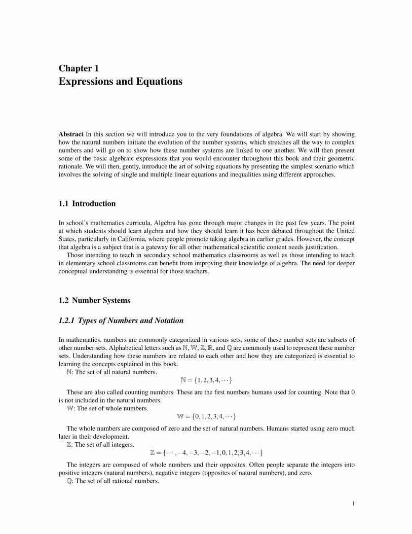
Find y-intercept: When x = 0, since 2x−3y =−12, then y = 4 is the y-interceptNow using X and Y intercepts we can draw the straight line 2x−3y =−12 corresponding to the equality.
Notice however since we have the strict inequality, then we must use a dotted line when drawing the line forthe final answer.Now we need to find which side of the line is the correct side for the inequality.Step 3: Identify the the correct side to shade.As before, consider (0,0) as a test point and plug it in.Plugging in x = 0 and y = 0, we get 0+0 >−12. Is this a true statement ? Yes, since 0 is greater than anynegative number.(0,0) is on the correct side !So, the correct side is the side of the straight line which contains (0,0). Now let us shade the final answer.
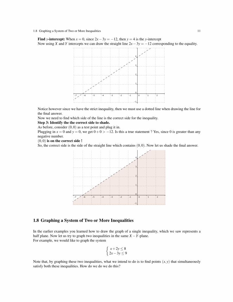
1.8 Graphing a System of Two or More Inequalities
In the earlier examples you learned how to draw the graph of a single inequality, which we saw represents ahalf plane. Now let us try to graph two inequalities in the same X−Y -plane.For example, we would like to graph the system{
x+2y≤ 82x−3y≤ 9
Note that, by graphing these two inequalities, what we intend to do is to find points (x,y) that simultaneouslysatisfy both these inequalities. How do we do we do this?

12 1 Expressions and Equations
First we find the region representing one of the inequalities using the method we used in the earlier exercises.Then we find the region representing the second inequality. Then we look to see whether there is a commonregion. That common region is the graph of the system of inequalities. We will try this in the following exam-ples.
Graphing a System of Two or More Inequalities: Worked out examples
1. Graph the system {x+2y≤ 8
2x−3y≤ 9
Answer: We will first draw the graph of the first inequality x+2y≤ 8.As before first consider x+2y = 8.x-intercept: Input y = 0. We get x = 8.y-intercept: Input x = 0. We get y = 4.Use the test point (0,0). We get 0 < 8, which is a true statement. Therefore (0,0) is on the correct side ofthe inequality. We get the following graph.
Next we draw the graph of the second inequality 2x−3y≤ 9.
When you draw these two regions in the same diagram, you will notice that there is a region that is commonto both these regions. This common region consists of the points (x,y) that simultaneously satisfy both theseinequalities. That common region is our solution, and it is called the feasible region of the system.The region common to both of the above regions (solution of the system) is shown below.

1.8 Graphing a System of Two or More Inequalities 13
2. Graph the system of inequalities {x+ y≤ 1y− x≤ 1
Answer: First we should graph the inequality x+ y ≤ 1, but this was already done in problem 1 of section1.7. We got the following graph:
Next we graph the inequality y− x ≤ 1 by graphing the line y− x = 1 and then plugging (0,0) into theinequality to decide which side to shade. We get:
So far we have individually graphed the two regions represented by the two inequalities. Now we simplygraph them in the same graph and find the common region:

14 1 Expressions and Equations
3. Find the region in the X−Y -plane common to y− x≤ 1, y+ x≥ 2, and x≤ 32
Answer: You will notice that the first two inequalities are the same as the last question but there is a thirdinequality this time. Since the first two were already graphed in the previous problem, let us just graph thethird.We want to graph the inequality x≤ 3
2 .Step 1. We change the ‘unequal’ sign to ‘equal’ and get x = 3
2 .Step 2. Next draw the line x = 3
2 . It is easy to see that this is a vertical line through x = 32
Now we need to find which side of the line is the correct side for the inequalityStep 3. To find the correct side, we select one side at random, and select a test point in that side. As before,consider (0,0) as a test point. We get 0≤ 3
2 , which is true. So (0,0) is on the correct side. Let us shade thisside.
So far we have individually graphed the three regions representing each of the three inequalities.

1.8 Graphing a System of Two or More Inequalities 15
When we draw all three regions in the same graph we see that the heavily shaded region in the picture belowis the region we are looking for
4. Find the region in the X−Y -plane common to 2y+3x > 6 and y− x≥ 1.Answer: A new thing in this problem is that the first inequality is a strict inequality. Hence, we will use adashed line when drawing the boundary of the region created by that inequality.We want to graph the inequality 2y+3x > 6.Step 1. The associated equation is 2y+3x = 6.Step 2. In order to graph this line we check the intercepts. The x-intercept is x = 2 and the y-intercept isy = 3. The graph of this line is shown below (notice the dotted line).

16 1 Expressions and Equations
Step 3. Take (0,0) as a test point. Plug it into 2y+3x > 6, we get 0 > 6, which is false. So, the correct sideis shown shaded below.
We want to graph the inequality y− x≥ 1.Step 1. The associated equation is y− x = 1.Step 2. In order to graph this line we check the intercepts. The x-intercept is x = −1 and the y-intercept isy = 1. The graph of this line is shown below.Step 3. Take (0,0) as a test point. Plug it into y− x≥ 1, we get 0 > 1, which is false. So, the correct side toconsider is shown shaded below.
Now we draw the two regions in a single graph and find the common region. You get the following region(shaded)

1.8 Graphing a System of Two or More Inequalities 17
5. Find a system of two linear inequalities having the region shaded below as a representation of its solution.
Answer: This problem asks you to do the reverse of the previous problem. Here, you are given the regionand asked to find the inequalities. To solve this problem you have to find the equations of the boundary lines.
(a) What is the equation of the continuous line?From the graph, you can see that the intercepts are (1,0) and (0,1). Now that you know these two points, youcan find the equation of the line. We use the slope formula to find the slope of the line through (x1,y1)= (1,0)and (x2,y2) = (0,1):
m =y2− y1
x2− x1=
1−00−1
=−1
The equation of the line in point-slope form is y− y1 = m(x− x1). By plugging in (x1,y1) = (1,0) andm =−1 we get y−0 = (−1)(x−1) which is y =−x+1.
(b) What is the equation of the dashed line?From the graph you can see that the intercepts are (−1,0) and (0,1). Now that you know these two points,you can find the equation of the line. We use the slope formula to find the slope of the line through (x1,y1) =(−1,0) and (x2,y2) = (0,1):
m =y2− y1
x2− x1=
1−00− (−1)
= 1
By plugging (x1,y1) = (1,0) and m = 1 into the point-slope formula, we get y−0 = (1)(x− (−1)) which isy = x+1.
(c) Now that we have the two equations how do we find the corresponding inequalities that we need?Let us take a test point from the (solution) region that is given to us (the region shaded). Notice that (−1,1)is in that region, so we plug this point into the expressions below to figure out what symbol should be in theboxes
y �− x+1 y � x+1
When we plug (−1,1) we get
1 <−(−1)+1 1 > (−1)+1
Since the equation y = −x+ 1 was associated with the continuous line, we get the inequality y ≤ −x+ 1.Similarly, the dashed line yields y > x+1. It follows that the system of the shaded region given is{
y≤−x+1y > x+1 i.e.
{y+ x≤ 1y− x > 1
6. Find the solution region of the system

18 1 Expressions and Equationsx+ y≤ 9
6x+4y≤ 48x≥ 0y≥ 0
Answer: This problem is more complex than the ones we have solved before because we have more in-equalities to consider for the solution region. However, the method used for previous problems works hereas well. We will streamline this process.
(a) Graph x+ y≤ 9
(b) Graph 6x+4y≤ 48
(c) Graph x≥ 0, which is what is to the right of the y-axis.

1.8 Graphing a System of Two or More Inequalities 19
(d) Graph y≥ 0, which is what is above the x-axis.
Putting all these graphs together at the same time we obtain the solution region for the system given
20 1 Expressions and Equations
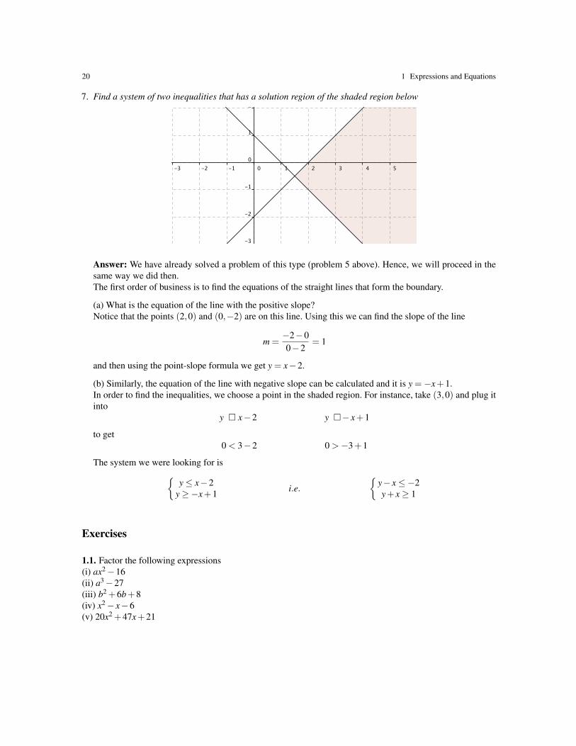
7. Find a system of two inequalities that has a solution region of the shaded region below
Answer: We have already solved a problem of this type (problem 5 above). Hence, we will proceed in thesame way we did then.The first order of business is to find the equations of the straight lines that form the boundary.
(a) What is the equation of the line with the positive slope?Notice that the points (2,0) and (0,−2) are on this line. Using this we can find the slope of the line
m =−2−00−2
= 1
and then using the point-slope formula we get y = x−2.
(b) Similarly, the equation of the line with negative slope can be calculated and it is y =−x+1.In order to find the inequalities, we choose a point in the shaded region. For instance, take (3,0) and plug itinto
y � x−2 y �− x+1
to get0 < 3−2 0 >−3+1
The system we were looking for is{y≤ x−2
y≥−x+1 i.e.{
y− x≤−2y+ x≥ 1
Exercises
1.1. Factor the following expressions(i) ax2−16(ii) a3−27(iii) b2 +6b+8(iv) x2− x−6(v) 20x2 +47x+21

1.8 Graphing a System of Two or More Inequalities 21
1.2. Graph (solve) the following inequalities.
(i){
y− x≥−1y+2x≤ 4 (ii)
{2x− y≤ 8x−3y≥ 6 (iii)
{2x+ y > 5
5x−3y < 15
(iv){
2x− y >−34x+ y < 5 (v)
{3x+2y≥ 15
x≥ 3 (vi)
2x−3y≤ 12x+5y≤ 20
x > 0
(vii)
x+3y≥ 123x+2y≤ 15
y≥ 2(viii)
2x+3y≥ 6y− x≥ 0
y≤ 2(ix)
4x+2y≥ 28
x≥ 0y≥ 0
2x+ y≥ 125x+8y≥ 74
(x)
x+6y≥ 24x≥ 0y≥ 0
1.3. Which of the following inequalities represent the region shaded below
(a){
8y−3x≥ 24y+2x≤ 10 (b)
{8y−3x≤ 24y+2x≥ 10
(c){
3x−8y≥−24y+2x≤ 10 (d)
{8y−3x≥ 24y+2x≥ 10
1.4. Write four systems of inequalities, one for each of the four regions in the X −Y -plane formed by thefollowing two lines.

Chapter 2Quadratic Equations
Abstract In this chapter we will discuss solving quadratic equations using both completing the square and thequadratic formula. Applications of the quadratic formula appear in SMR 1.2 of the CSET subtest 1 examination.
A quadratic equation is an equation of the form ax2 +bx+ c = 0, where a 6= 0 and a,b, and c could be realor complex numbers. There are many ways to solve such an equation, and there are many problems that canbe solved by using quadratic equations. In this chapter you will learn, among other things, the following topicsregarding quadratic equations
1. How to solve a given quadratic equation using the quadratic formula.2. How to solve a quadratic equation using completing the square.3. How to solve a rational equation, which leads to a quadratic equation.4. How to solve an equation, which can be transformed into quadratic equations.5. How to handle a quadratic equation with complex coefficients6. How to manipulate the roots of a quadratic equation without solving the equation.
2.1 The Quadratic Formula
The quadratic formula is the name we give to the formula that says that the solutions of the equation ax2+bx+c = 0, where a 6= 0, are given by
x =−b±
√b2−4ac
2a
The number ∆ = b2−4ac is called the discriminant of the equation ax2 +bx+ c = 0. Since computing√
∆
yields either two distinct real numbers (when ∆ > 0), or one real number (which is zero, when ∆ = 0), or twodistinct complex (no real) numbers (when ∆ < 0) then
• if ∆ > 0, then the equation has exactly two distinct real solutions,• if ∆ = 0, then the equation has exactly one real solution,• if ∆ < 0, then the equation has exactly two distinct complex (non-real) solutions.
If you want to use the quadratic formula to solve a given quadratic equation you can use a two-step approach:Step 1. Write the given equation in the standard form: ax2 +bx+ c = 0.Step 2. Identify what a, b and c are, and the plug these values in the quadratic formula to get the solution(s).
The Quadratic Formula: Worked out examples
1. Solve x2−5x+6 = 0.Answer: Since this equation is already in standard form, we can immediately go to step 1 and find a,b andc. In this case we get a = 1, b =−5 and c = 6.Now we plug these values into the quadratic formula and obtain
x =−(−5)±
√(−5)2−4(1)(6)2(1)
=5±√
25−242
=5±1
2
23

24 2 Quadratic Equations
We get the solutions to be x =5−1
2= 2 and x =
5+12
= 3.Notice also that in this case the discriminant ∆ = 1 > 0, which means the equation has two distinct realroots. This is consistent with what we have found above.
2. Solve x2 = 2−4x.Answer: This equation is not yet in standard form, so we need to put it in the standard, which is x2+4x−2=0.Now we look for the values to plug into the quadratic formula, and we get a = 1, b = 4 and c = −2. Byplugging these values we obtain
x =−(4)±
√(4)2−4(1)(−2)2(1)
=−4±
√16+8
2=−4±
√24
2=−4±2
√6
2=−2±
√6
So, the solutions are x =−2−√
6 and x =−2+√
6.3. Solve x2 +8x+16 = 0.
Answer: This equation is already in standard form, so we just identify a = 1, b = 8 and c = 16. We plugthese values into the quadratic formula to obtain
x =−(8)±
√(8)2−4(1)(16)2(1)
=−8±
√64−64
2=−8±
√0
2=−4
So, there is only one solution, which is x = −4. Note that this is consistent with having ∆ = 0 for thisequation.
4. Solve x2−2x+2 = 0.Answer: Since this equation is already in standard form, then we start by identifying a = 1, b = −2 andc = 2. We plug these values into the quadratic formula to obtain
x =−(−2)±
√(−2)2−4(1)(2)2(1)
=2±√
4−82
=2±√−4
2=
2±2√−1
2= 1±
√−1
Since√−1 = i, the we get two complex roots: x = 1− i and x = 1+ i. Note that this is consistent with having
∆ =−4 < 0 for this equation.5. Solve the equation (x+2)(x+1) = 12.
Answer: Even though this equation does not seem to be a quadratic equation, it is. In order to see this onejust needs to multiply the expression on the left-hand side. Let us do this
12 = (x+2)(x+1) = x2 +3x+2
and thus, the equation we want to solve is x2 +3x−10 = 0.Now we just plug a = 1, b = 3 and c =−10 into the quadratic formula to obtain
x =−(3)±
√(3)2−4(1)(−10)
2(1)=−3±
√9+40
2=−3±
√49
2=−3±7
2
So, we get the two solutions to be x =−5 and x = 2.
2.2 Rational Equations That Lead to Quadratic Equations
Consider the equation
8−4x =1x

2.3 Quadratic Equations With Complex Coefficients 25
At first sight, this does not look like a quadratic equation. But if you multiply both sides of the equation by xthen you do get the following quadratic equation:
8x−4x2 = 1
So, in order to solve a rational equation one should try to multiply both sides of the equation by an expressionthat eliminates all denominators (multiplying by the LCM of the denominators is a good idea). After multiplyingand simplifying you might end up with a quadratic equation, which you can solve using steps 1 and 2 that weoutlined in the previous section.
Rational Equations That Lead to Quadratic Equations: Worked out examples
1. Solve 8−4x =1x
.
Answer: As we have seen above, after multiplying by x both sides of this equation we get 8x− 4x2 = 1,which once re-written as 8x−4x2−1 = 0 we can solve by setting a = 8, b =−4, and c =−1 and pluggingthese values in the quadratic formula to get
x =−(−4)±
√(−4)2−4(8)(−1)2(8)
=4±√
4816
=4±4
√3
16=
1±√
34
Therefore the solutions are x =1−√
34
and x =1+√
34
.
2. Solvex−2x−3
= x+2.
Answer: In this case, we need to multiply both sides by x− 3 to eliminate all denominators. Once we dothis we get
x−2 = (x+2)(x−3)
which can be re-written by multiplying the terms on the right-hand side to get x−2 = x2−x−6, which aftersimplifying becomes, x2−2x−4 = 0Since in this case we have a = 1, b =−2, and c =−4 then
x =−(−2)±
√(−2)2−4(1)(−4)2(1)
=2±√
202
=2±2
√5
2= 1±
√5
So, the solutions are x = 1−√
5 and x = 1+√
5.
2.3 Quadratic Equations With Complex Coefficients
As mentioned at the beginning of this chapter, the coefficients a,b and c of the equation ax2 +bx+c = 0 couldbe real or complex. So far we have solved only equations with real coefficients, but in this section we willdiscuss equations that might have complex coefficients. In short, there is no need to worry about this ‘strange’numbers, you should proceed as if you were solving a quadratic equation with real coefficients.
Example 2.1. We want to solve z2 +(2− i)z− i = 0.Comparing with the standard quadratic equation ax2 + bx+ c = 0 (of course now we have the variable z
instead of x) we see that a = 1, b = 2− i, and c =−i then

26 2 Quadratic Equations
z =−(2− i)±
√(2− i)2−4(1)(−i)2(1)
=−2+ i±
√22−2 ·2i+(i2)+4i
2
=−2+ i±
√3
2
So, we have two solutions for the equation: z =−2−
√3+ i
2and z =
−2+√
3+ i2
.
Quadratic Equations With Complex Coefficients: Worked out examples
1. Find the imaginary part of the solutions of 2iz2 +(4+ i)z+1 = 0.Answer: In order to find the imaginary part of the solutions of the equation, we first need to solve theequation. It is clear that a = 2i, b = 4+ i, and c = 1 then
z =−(4+ i)±
√(4+ i)2−4(2i)(1)2(2i)
=−4− i±
√(16+8i−1)−8i
4i
=−4− i±
√15
4i
Now to find the imaginary parts, first we notice that i appears both in the numerator and the denominator.To get rid of the 4i in the denominator we will multiply both the numerator and the denominator by −4i.Hence,
z =(−4− i±
√15)(−4i)
−(4i)2
=16i+4i2±
√15 4i
16
=−4+(16±4
√15)i
16
=−416
+16±4
√15
16i
It follows, after simplifying, that the imaginary parts of the roots are4±√
154
.
2. Find the solutions, and their imaginary parts, for z2 +2z+4i−2 = 0.Answer: It is clear that a = 1, b = 2, and c = 4i−2. Thus, the quadratic formula yields
z =−(2)±
√(2)2−4(1)(4i−2)
2(1)
=−2±
√4(3−4i)2
= −1±√
3−4i
In any one of the previous problems we have ever had a non-real number under the the radical sign. Whatdo we do with that 3−4i under the radical? Well, our best hope is that 3−4i is a square, in which case the

2.4 Equations That Transform Into Quadratic Equations 27
radical would cancel with the square and then we would have a clean expression, with no square roots. Letus see if we can get 3−4i to be square.Since (s+ ti)2 = (s2− t2)+2sti then we want to find s and t such that 3 = s2− t2 and −4 = 2st. We see thats = 2 and t =−1 solve these equations, and thus (2− i)2 = 3−4i. Hence, the solutions of the equation are
z =−1±√
3−4i =−1±√
(2− i)2 =−1± (2− i)
which, explicitly, are x =−3+ i and x = 1− i.
2.4 Equations That Transform Into Quadratic Equations
Consider the problem of solving the equation x4−5x2 +4 = 0, which is an equation of degree 4.Note that by using the simple substitution t = x2 we can transform this equation into a quadratic equation.
In fact, we gett2−5t +4 = 0
which has solutions t = 1 and t = 4. Hence, the solutions for the original equation are given by x2 = 1 andx2 = 4. This implies that the solutions are x =±1 and x =±2.
Equations That Transform Into Quadratic Equations: Worked out examples
1. Solve x4−13x2 +36 = 0.Answer: Using the substitution t = x2 we obtain the equation t2−13t +36 = 0, which we can solve usingthe quadratic formula, we get
t =13±
√(−13)2−4 ·36
2=
13±52
It follows that the solutions for this equation are t = 4 and t = 9. So, we now know that x2 = 4 and x2 = 9,and thus x =±2 and x =±3.
2. Solve x2/3−3x1/3 +2 = 0.Answer: In this equation setting t = x2 will lead us nowhere, but since x2/3 = (x1/3)2 then we can considerthe substitution t = x1/3 to get the equation.
t2−3t +2 = 0
Now we use the quadratic formula to find the solutions to this equation. We get t = 1 and t = 2. It followsthat x1/3 = 1, and thus x = 1 or x1/3 = 2, and thus x = 8.Since this is a radical equation it is of vital importance to check whether the solutions found are correct. Wecheck:For x = 1
12/3−3 ·11/3 +2 = 1−3+2 = 0
For x = 882/3−3 ·81/3 +2 = 4−3 ·2+2 = 4−6+2 = 0
So, both x = 1 and x = 8 are valid solutions.3. Solve a−6
√a+8 = 0.
Answer: This is just like the previous example except that in this case we will use you the substitutiont =√
a, which will transform the given equation into t2−6t+8= 0, which can be solved using the quadraticformula. The solutions of this equation are t = 2 and t = 4. Now we back-substitute to get
√a= 2 and
√a= 4
implying a = 4 and a = 16.It is easy to check that both solutions make sense and are valid.

28 2 Quadratic Equations
2.5 Manipulation of Roots of Quadratic Equations
Sometimes it becomes necessary for us to get information about the roots of a quadratic equation withoutactually solving the equation. In order to do this we will use a couple of very simple formulas.
Let α and β be the two solutions (not necessarily distinct) of the equation ax2 +bx+ c = 0, then:
(i) α +β =−ba
(ii) αβ =ca
(iii) |α−β |=√
∆
a
where ∆ = b2−4ac, the discriminant of the equation.Why does all this make sense? Note that if α and β are the two solutions of ax2 +bx+ c = 0 then
ax2 +bx+ c = a(x−α)(x−β )
and thus, when multiplying the expression on the right we get
ax2 +bx+ c = ax2−a(α +β )x+aαβ
By comparing the coefficients with x and no x we get the α +β =−ba
and αβ =ca
.
The expression |α−β |=√
∆
afollows from taking the difference of the solutions given by the quadratic
formula, that is
|α−β |=∣∣∣∣∣−b+
√b2−4ac
2a− −b−
√b2−4ac
2a
∣∣∣∣∣=∣∣∣∣∣±√
b2−4aca
∣∣∣∣∣=√
b2−4aca
Manipulation of Roots of Quadratic Equations: Worked out examples
1. Find the sum and the product of the roots of the equation 4x2−8x+3 = 0.Answer: This can be calculated easily by simply plugging values in the formulae given.
α +β =−ba=−−8
4= 2 αβ =
ca=
34
2. Find the absolute value of the difference of the roots of the equation 4x2−16x+15 = 0.Answer: Then again, from the formulae given above, we can calculated this easily
|α−β |=√
(16)2−4 ·4 ·154
=
√164
= 1
2.6 Solving Quadratic Equations by Completing the Square.
Using the quadratic formula is one way of solving a quadratic equation. Another way is to use a method calledcompletion of a square. We will describe this method in the following steps.
Assume the quadratic equation has the form ax2 +bx+ c = 0.Step 1: Subtract the constant c from both sides so that only the x2 and x terms are left on the left-hand side.Step 2: Make the coefficient of x2 equal to 1 by dividing both sides by the coefficient a. Note that now thecoefficient of x has also been modified.
Step 3: Add(
12·new coefficient with x
)2
both sides.

2.6 Solving Quadratic Equations by Completing the Square. 29
Step 4: Write the left hand side as a complete square. You should have(x− 1
2·new coefficient with x
)2
Step 5: Take square roots on both sides. Make sure to put ± on front of the radical.Step 6: Solve for x.
Solving Quadratic Equations by Completing the Square: Worked out examples
1. Solve x2 +6x+5 = 0 by completing the square.Answer: Let us perform the steps described above.Step 1: Subtract 5 both sides: x2 +6x =−5Step 2: Since the coefficient with x2 is 1, there is nothing to do.Step 3: 1/2 of the coefficient with x is 3, then we add 32 = 9 both sides: x2 +6x+9 = 4Step 4: The left-hand side is a perfect square: (x+3)2 = 4.Step 5: We take square roots both sides: x+3 =±2.Step 6: x =−3±2, and thus x =−1 or x =−5.
2. Solve 2x2 +6x−3 = 0 by completing the square.Answer: Just as in the previous problem, we will perform the steps described above.Step 1: Subtract −3 both sides: 2x2 +6x = 3
Step 2: The coefficient with x2 is 2, then we divide by 2: x2 +3x =32
Step 3: 1/2 of the coefficient with x is32
, then we add(
32
)2
both sides, we get
x2 +3x+(
32
)2
=32+
(32
)2
Step 4: The left-hand side is a perfect square, and we simplify the right-hand side:(x+
32
)2
=154
Step 5: We take square roots both sides: x+32=±
√154
.
Step 6: x =±√
154− 3
2=−3±
√15
2
3. Solve x(2x−1) =−72
by completing the square.
Answer: We first distribute and get the equation in the standard form: 2x2− x+72= 0. Now we can use the
steps.
Step 1: Subtract72
both sides: 2x2− x =−72
Step 2: The coefficient with x2 is 2, then we divide by 2: x2− 12
x =−74
.
Step 3: 1/2 of the coefficient with x is14
, then we add(
14
)2
both sides, we get
x2− 12
x+(
14
)2
=−74+
(14
)2
Step 4: The left-hand side is a perfect square, and we simplify the right-hand side:
30 2 Quadratic Equations(x− 1
4
)2
=−2716
Step 5: We take square roots both sides: x− 14=±
√−27
16.
Step 6: x =14±√−27
16=
1±3√−3
4=
1±3√
3i4
Exercises
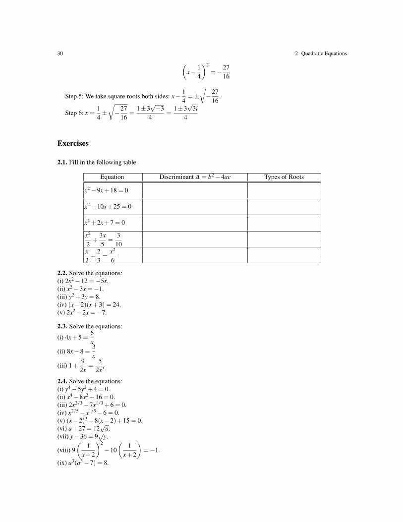
2.1. Fill in the following table
Equation Discriminant ∆ = b2−4ac Types of Roots
x2−9x+18 = 0
x2−10x+25 = 0
x2 +2x+7 = 0
x2
2+
3x5
=3
10x2+
23=
x2
6
2.2. Solve the equations:(i) 2x2−12 =−5x.(ii) x2−3x =−1.(iii) y2 +3y = 8.(iv) (x−2)(x+3) = 24.(v) 2x2−2x =−7.
2.3. Solve the equations:
(i) 4x+5 =6x
(ii) 8x−8 =3x
(iii) 1+92x
=5
2x2
2.4. Solve the equations:(i) y4−5y2 +4 = 0.(ii) x4−8x2 +16 = 0.(iii) 2x2/3−7x1/3 +6 = 0.(iv) x2/5− x1/5−6 = 0.(v) (x−2)2−8(x−2)+15 = 0.(vi) a+27 = 12
√a.
(vii) y−36 = 9√
y.
(viii) 9(
1x+2
)2
−10(
1x+2
)=−1.
(ix) a3(a3−7) = 8.

2.6 Solving Quadratic Equations by Completing the Square. 31
2.5. Find the solutions of(i) z2−2iz−3 = 0.(ii) iz2 +(1−5i)z−1+8i = 0.
2.6. Find the imaginary parts of the solutions of iz2 +3z−2i = 0.
2.7. What are the real and imaginary parts of the solutions of the equation
(1+ i)z2 +(3−2i)z− (21−7i) = 0 ?
2.8. If α and β are the solutions of the equation x2−2x−3 = 0. Find
(i) αβ (ii)α +β (iii)|α−β | (iv)α2 +β2
2.9. Find the absolute value of the difference of the roots of the equation 2x2− x−3 = 0.
2.10. You are given that the absolute value of the difference of the roots of x2−mx+ 1 = 0 is equal to√
5,where m is a real positive number. Find m.
2.11. Solve the following quadratic equations by completing squares(i) x2 +4x = 9.(ii) 2x2−4x−1 = 0.(iii) 6x = 1−4x2.(iv) x(2x+9) =−5.

Chapter 3Relations and Functions
Abstract In this chapter we will discuss the concepts related to relations and functions. This content is used inthe CSET 1 examination SMR 1.3
3.1 Relations
A relation is created when the elements of two sets are related. Consider the following two sets:
Years = { 2003, 2004, 2005, 2006, 2007} Teams = {Spurs, Pistons, Heat}
and the relation is given by the figure below
Advanced Algebra for Teachers 93
!"#$%&'()(*(+&,#%-./0(#/1(23/4%-./0( In this chapter we will discuss the concepts related to relations and functions. Is content is used in the CSET 1 examination SMR 1.3
)56(+&,#%-./0(A relation is created when the elements of two sets are related. Consider the following two sets:
Years={2003, 2004, 2005, 2006,2007} Teams={Spurs, Pistons, Heat}
And the relation is given by the map below. You can clearly see that the relation above relates the year to the team that won the NBA Championship. We can also write the relation as a collection of ordered pairs {(2003, Pistons), (2004, Spurs), (2005, Heat), (2006, Heat), (2207, Spurs)} The Domain and the range of a relation Notice that in the above relation, the set of years ={2003,2004,2005,2006,2007} served
The Domain of a relation is the set of inputs for the relation while the range of a relation is the set of outputs of the relation. So for the above relation,
Domain={2003, 2004, 2005, 2006, 2007}. Range={Spurs, Pistons, Heat}
Notice that in the Range, we do not repeat "Spurs" twice even though it repeats twice as an output in the relation. The reason for this is the when you are writing a set, you are not allowed to repeat elements.
2003 2004 2005 2006 2007
Spurs Pistons Heat
You can clearly see that the relation above relates a year to the team that won the NBA Championship thatyear. We can also write the relation as a collection of ordered pairs
{(2003, Pistons), (2004, Spurs), (2005, Heat), (2006, Heat), (2207, Spurs)}
3.1.1 Domain and Range of a Relation
Notice that in the above relation, the set of years, {2003,2004,2005,2006,2007}, served as a set of ‘inputs’,while the set {Spurs, Pistons, Heat} served as a set of ‘outputs’. The domain of a relation is the set of inputsfor the relation while the range of a relation is the set of outputs of the relation. So for the above relation,
Domain={2003, 2004, 2005, 2006, 2007} Range={Spurs, Pistons, Heat}
Notice that in the range, we do not write ‘Spurs’ twice even though they won two championships, and thusthey appear twice as an output of the relation. The reason for this is the when you are writing a set, you are notallowed to repeat elements. Also, notice that it is OK have the same output for multiple inputs. The reverse isalso true for relations as we can see in our example below.
33

34 3 Relations and Functions
Domain and Range of a Relation: Worked out examples
1. Find the domain and range of the following relation which matches some western states with their senators(as of 2010). Then write the relation as a set of ordered pairs.
Advanced Algebra for Teachers 94
Also notice that it is OK have the same output for multiple inputs. The reverse is also true for relations as we can see in our example below. Relations Worked out examples
Example 1. Find the domain and the following relation which matches some western states with their senators (as of 2010) and write the relation as a set of ordered pairs.
Solution
Notice that in the above relation, each input has two outputs. That is perfectly OK for a relation.
Domain=The set of inputs = {CA, OR, NV} Range= The set of outputs= { Barbara Boxer, Dianne Feinstein, Jeff Merkley, Ron Wyden, John Ensign, Harry Reid}
The relation as a collection of ordered pairs ={(CA, Barbara Boxer),(CA, Dianne Feinstein),(OR, Jeff Merkley),(OR, Ron Wyden),(NV, John Ensign),(NV, Harry Reid)}.
Example 2. Write down the domain and the range of the relation given below and represent it as a figure.
Solution.
Notice that in this problem, the relation is given to you as a set of ordered pairs.
CA OR NV
Barbara Boxer Dianne Feinstein Jeff Merkley Ron Wyden John Ensign Harry Reid
Answer: Notice that in the above relation, each input has two outputs. That is perfectly OK for a relation.We have:Domain = set of inputs = {CA, OR, NV}.Range = set of outputs= {Barbara Boxer, Dianne Feinstein, Jeff Merkley, Ron Wyden, John Ensign, HarryReid}.The relation as a collection of ordered pairs is = {(CA, Barbara Boxer), (CA, Dianne Feinstein), (OR, JeffMerkley), (OR, Ron Wyden), (NV, John Ensign), (NV, Harry Reid)}.
2. Write down the domain and range of the relation given below and represent it as a figure.
{(2,8), (5,−2), (7,12), (−4,−7), (7,3), (5,−1)}
Answer: Notice that in this problem, the relation is given to you as a set of ordered pairs. Let us firstrepresent it by using a diagram.
Advanced Algebra for Teachers 95
Domain= The set of inputs ={-4,2,5,7} Range=The set of outputs={-7,-2,-1,3,8,12}
Example 3. Identify the domain and the range of the relation given in the graph below.
Solution
t that we have plotted the ordered pairs as points in the X-Y plane. In this type of
!"
!#
!$
!%
&
%
$
#
"
!" !# !$ !% & % $ # "
-4 2 5 7
-7 -2 -1 3 8 12
It follows that the domain is {−4,2,5,7} and the range is {−7,−2,−1,3,8,12}.

3.1 Relations 35
3. Identify the domain and range of the relation given in the graph below.
Advanced Algebra for Teachers 95
Domain= The set of inputs ={-4,2,5,7} Range=The set of outputs={-7,-2,-1,3,8,12}
Example 3. Identify the domain and the range of the relation given in the graph below.
Solution
t that we have plotted the ordered pairs as points in the X-Y plane. In this type of
!"
!#
!$
!%
&
%
$
#
"
!" !# !$ !% & % $ # "
-4 2 5 7
-7 -2 -1 3 8 12
Answer: In this example, the relation is given as a graph. It is the same concept explored before, exceptthat we have now plotted the ordered pairs as points in the X −Y -plane. In this type of problem, the set ofx-coordinates of the points of the graph are the inputs of the relation, and the set of y-coordinates of thepoints of the graph are the outputs of the relation.We get the relation
{(−3,2),(−2,−1),(0,2),(0,−3),(2,−1),(3,3)}and thus
Domain = {-3,-2,0,2,3} Range = {2,-1,-3,3}Notice that once again we have not repeated the elements when writing the domain and range.
4. Graph the relation y =−x2 +1 and use the graph to determine its domain and range.Answer: In this example, think of x as the input and y as the output. To draw the graph, we first need tocalculate some ordered pairs, which represent the function. In order to do that let us create a table.
x y =−x2 +1 (x,y)−3 −(−3)2 +1 =−8 (−3,−8)−2 −(−2)2 +1 =−3 (−2,−3)−1 −(−1)2 +1 = 0 (−1,0)0 −(0)2 +1 = 1 (0,1)1 −(1)2 +1 = 0 (1,0)2 −(2)2 +1 =−3 (2,−3)3 −(3)2 +1 =−8 (3,−8)
The corresponding graph follows

36 3 Relations and Functions
By looking at the graph, we can observe the following.- The inputs can take any x value! (We only took from −3 to 3, just to draw the graph). You could, if youwanted, plug any real number x into y = −x2 + 1 and always get a corresponding value for y. Therefore,Domain = all real numbers = (−∞,∞).- You can clearly see that that outputs (y values) cannot exceed 1. Therefore, the range is the set of all realnumbers less than or equal to 1, which is {y; y≤ 1}= (−∞,1].
3.2 What is a Function?
Now if you compare the ‘NBA’ relation and the ‘Senator’ relation that we presented in the previous section, wecan see that one of the key differences between these two relations is that, in the ‘NBA’ relation, each input hasonly one output but in the ‘Senator’ relation some inputs have multiple outputs. For instance, the input ‘CA’has two outputs, namely Barbara Boxer and Dianne Feinstein.
A function is a special type of relation where each number in the input set is mapped to one single output.Therefore, the ‘NBA’ relation is a function while the ‘Senator’ relation is not.
What is a Function?: Worked out examples
1. The following relation maps a group of students to their birthday. Is this relation a function?
Advanced Algebra for Teachers 98
A function is a special type of relation where each number in the input set is mapped to one single output.
Definition of a function Worked out examples
Example 1. The following relation maps a group of students to their birthday. Is this relation a function?.
Solution
Notice that each input is mapped to one single output. Therefore, this is a function. Two inputs (Steve and Amanda) have a single output. This is OK.
Example 2. Determine whether each of the following relations determine a function and if so, find the Domain and the Range of the function.
a) b) c)
Solution (a) This is a function. Domain of function=Domain of relation={-4,-3,-
2,0,1,2}. The range of the function={3,2,5,6}. Notice that all three inputs -4,-2 and 0 have a single output (3). But this is perfectly OK for a function as long as no input has multiple outputs,
Steve Judy Alicia Amanda
June 10 May 10 April 1
Answer: Since each input is mapped to one single output then this is a function. Notice that two inputs(Steve and Amanda) have a single output. This is OK, we have no restrictions for this type of situation.
2. Determine whether each of the following relations determine a function and if so, find their domain andrange.(a) {(−4,3), (−3,2), (−2,3), (0,3), (1,5), (2,6)}(b) {(−2,2), (−1,4), (0,5), (1,7), (2,8)}(c) {(−2,2), (−2,4), (−1,2), (0,3), (4,7)}
Answer: (a) Since every input yields a unique output then this is a function. The domain of this function is{−4,−3,−2,0,1,2} and its range is {3,2,5,6}. Notice that all three inputs −4,−2 and 0 have a commonoutput, namely 3. This is perfectly OK for a function, we do not have any restrictions of this type forfunctions.(b) Again this is a function. Domain= {-2,-1,0,1,2}. Range={2,4,5,7,8}.(c) This is not a function since the input −2 has two outputs: 2 and 4. This is not allowed for a function.
3. Determine whether each of the following relations determine a function.(a) y = 3x
3.3 The Domain of a Function 37
(b) y =±3x(c) y2 = x
Answer: In the problems above, the relation is given by an equation. As we did in the previous section,think of x as the input and y as the output to see if these relations are functions.a) When you give a value for x, the value of y is determined by y = 3x, which is a unique value. So, this is afunction.b) Let x = 1. Then y =±3. That is, you get two (output) values for x = 1. Therefore, this is not a function.c) Let x = 4. then y2 = 4, which implies that y = ±2. This means that there are two (output) values for theinput x = 4. This cannot be a function.
A function can be presented in many different ways. Many times, it will be given by a ‘formula’. What doesthis mean? Let us say that f is our function and let x be an element in the domain of the function. Then theelement in the range which corresponds to x is called f (x) and is pronounced ‘ f of x’. For example, the functiony = 3x, that we encountered in example 3 in section 3.2, can be written as f (x) = 3x. In this context, x is calledthe independent variable and y is called the dependent variable.
Example 3.1. Let f be the function given by f (x) = x2 +3x+2. We want to find the values of
(a) f (−2) (b) f (3) (c) f (a) (d) f (a+h)
(a) In order to find f (−2), we simply substitute −2 for x in the function definition. We get
f (−2) = (−2)2 +3(−2)+2 = 4−6+2 = 0
(b) In order to find f (3), we substitute 3 for x in f (x) = x2 +3x+2. We get
f (3) = (3)2 +3(3)+2 = 9+9+2 = 20
(c) Now we just substitute a for x and get f (a) = a2 +3a+2.(d) In order to find f (a+h), we substitute a+h for x in f (x) = x2 +3x+2. We get
f (a+h) = (a+h)2 +3(a+h)+2 = a2 +2ah+h2 +3a+3h+2
3.3 The Domain of a Function
When a function is explicitly given as a relation, then the domain of the function is simply the domain of therelation, which is just the set of inputs. However, if we were given a function f (x) as a ‘formula’ without anyindications on the input set, then we should be able to decide what the domain of f (x) is. What we do is thatwe take the domain of f (x) to be the largest set numbers for which f (x) can be computed (it has an output).For example if f (x) = 1
x−3 , then you will see that the only number that x cannot be equal to is 3. Therefore, thedomain of f (x) consists of all real numbers other than 3.
In the search for values that are not in the domain of a function we should remember the following:- a radical (of an even root) of a negative number is not a real number- a fraction with a zero in the denominator is not defined.
Hence, when looking for the domain of a function, let us always ask ourselves these questions to start with:- Does the function have denominator? If yes, then you should check for which values the denominator becomeszero. All these values must be removed from the domain. If not, then no problems there!- Does the function have a radical? If yes, then you must make sure that what is inside the radical (even indexonly) is not negative. Remove points that yield a negative radical (even index) If not, then no problems here!

38 3 Relations and Functions
Example 3.2. We want to find the domain of each of the functions given below.
(a) f (x) =√
x−3 (b) g(x) =1
x2−9(c) h(x) = x2 +5
(a) Since this function is not a fraction then we do not need to worry about zeros in the denominator. However,this function has a square root, and thus (x− 3) must be positive. We set x− 3 ≥ 0, which implies x ≥ 3. So,the domain of f (x) is {x; x≥ 3}.(b) Because there are no radicals in this function, then we only have to worry about zero in the denominator. Itfollows that x2−9 6= 0. Since the equation x2−9 = 0 has solutions x =±3, then 3 and−3 are the only ‘illegal’points and should be removed from the domain. Hence, the domain of g(x) is the set of all real numbers except±3.(c) Since the functions has neither denominators nor radicals, there are no ‘problematic’ values for x. So, x cantake any value, and thus the domain of h(x) is the set of all real numbers.
3.4 The Graph of a Function
The graph of a function f is defined as the collection of points x, f (x)), where x is any point in the domain ofthe f . In other words it is the collection of the (input, output) pairs of the function displayed in the X−Y -plane.
Example 3.3. We want to sketch the graph of the function f (x) =√
x−1.There are many ways to sketch the graph of a function. The easiest way is to plot a few points and then join
them with a curve. Notice that the domain of the function (because there is a squared root), is {x; x ≥ 1}. So,when we are drawing the table, we must only consider values for x that are at least 1.
x y =√
x−1 (x,y)1
√1−1 = 0 (1,0)
2√
2−1 = 1 (2,1)3
√3−1 =
√2∼ 1.414 (3,1.414)
4√
4−1 =√
3∼ 1.732 (4,1.732)5
√5−1 = 2 (5,2)
We now plot these points on the X−Y -plane and get
At the beginning of this problem we saw that the domain of this function is {x; x≥ 1}. From the graph wecan clearly see that the outputs of f (x) can only take values y≥ 0. Therefore, the range of f (x) is the set of allpositive real numbers.

3.5 Algebra of Functions 39
3.4.1 The Vertical Line Test.
Sometimes, as we saw in section 3.1, a relation can be presented as a graph. To determine whether such arelation defines a function, we can use the vertical line test.
The vertical line testA collection of points representing a relation in the X −Y -plane is a function if and only if each vertical linedrawn on the X−Y -plane cuts the graph at most once. That is, it is OK to not cut the graph, to cut it at exactlyone point, but it is not OK to cut the graph at two or more points.
Example 3.4. Let us use the vertical line test to determine whether the following graphs represent functions.
(a) (b) (c)
(a) A vertical line drawn will cut the graph in two places most of the times. So, the graph does not represent afunction.(b) Any vertical line will only cut the graph at one place. Therefore, this represents a function.(c) A vertical line will cut the graph at two places most of the times. So, the graph does not represent a function.
3.5 Algebra of Functions
In this section we will discuss operations between functions. That is, ways of obtaining new functions out ofknown ones. These operations include sum, difference, product, quotient, and composition of functions.
Let f and g be two functions. We can define the sum, difference, product and quotient of these two functionsby:
• Sum: ( f +g)(x) = f (x)+g(x).• Difference: ( f −g)(x) = f (x)−g(x).• Product: ( f g)(x) = f (x)g(x).
• Quotient:(
fg
)(x) =
f (x)g(x)
.
Note that the domains of f + g, f − g, and f g are the intersections of the domains of f and g, but that the
domain offg
is the intersection of the domains of f and g excluding the points x such that g(x) = 0.
Example 3.5. We want to find the sum, difference, product and quotient of the functions f (x) =√
x+2 andg(x) = 3x+1.
The definitions above tell us
• Sum: ( f +g)(x) = f (x)+g(x) =√
x+2+3x+1.• Difference: ( f −g)(x) = f (x)−g(x) =
√x+2− (3x+1).
• Product: ( f g)(x) = f (x)g(x) =√
x+2(3x+1).
• Quotient:(
fg
)(x) =
f (x)g(x)
=
√x+2
3x+1.
Note that in the last function we need 3x+1 6= 0, that is x 6=− 13 .
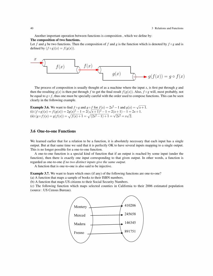
40 3 Relations and Functions
Another important operation between functions is composition , which we define by:The composition of two functions.Let f and g be two functions. Then the composition of f and g is the function which is denoted by f ◦g and isdefined by ( f ◦g)(x) = f (g(x)).
x
f (x)
g(f (x)) = g ! f (x)
f (x)
g(x)
The process of composition is usually thought of as a machine where the input x, is first put through g andthen the resulting g(x) is then put through f to get the final result f (g(x)). Also, f ◦g will, most probably, notbe equal to g◦ f , thus one must be specially careful with the order used to compose functions. This can be seenclearly in the following example.
Example 3.6. We want to find f ◦g and g◦ f for f (x) = 2x2−1 and g(x) =√
x+1.(i) ( f ◦g)(x) = f (g(x)) = 2g(x)2−1 = 2(
√x+1)2−1 = 2(x+1)−1 = 2x+1.
(ii) (g◦ f )(x) = g( f (x)) =√
f (x)+1 =√(2x2−1)+1 =
√2x2 = x
√2.
3.6 One-to-one Functions
We learned earlier that for a relation to be a function, it is absolutely necessary that each input has a singleoutput. But at that same time we said that it is perfectly OK to have several inputs mapping to a single output.This is no longer possible for a one-to-one function.
A one-to-one function is a special kind of function that if an output is reached by some input (under thefunction), then there is exactly one input corresponding to that given output. In other words, a function isregarded as one-to-one if no two distinct inputs give the same output.
A function that is one-to-one is also said to be injective.
Example 3.7. We want to learn which ones (if any) of the following functions are one-to-one?(a) A function that maps a sample of books to their ISBN numbers.(b) A function that maps US citizens to their Social Security Numbers.(c) The following function which maps selected counties in California to their 2006 estimated population(source : US Census Bureau).
Advanced Algebra for Teachers 106
Therefore . Now let us find . By definition
. To find this now we substitute for in we get
!Therefore
!"#$$%&'$()$)&'$*+&,(-)&."$We learnt earlier that for a relation to be a function, it is absolutely necessary that each input has only one single output. But at that same time we told that it is perfectly OK to have several inputs mapping to a single output. Now a one to one function is a special kind of function where even this is not allowed. A one to one function has only one input corresponding to a given output. In other words a function is regarded as one-to-one if no two inputs give the same output.
Section 5.8 One-to-One functions
Worked out examples
Example 1. Which one of the following maps are one-to-one ?
a) A map which maps a sample of books to their ISBN numbers. b) A map which maps US citizens to their Social Security numbers. c) The following function which maps selected counties in California to their 2006
estimated population (source : US Census Bureau)
Montery Merced Madera Fresno
410206 245658 146345 891751

3.6 One-to-one Functions 41
(d) The ‘NBA function’ discussed in section 3.1.
In order to do this we will check whether ‘no two inputs give the same output’. If so, the function is one-to-one. Otherwise it is not.(a) This function is one-to-one since no two books (inputs) can have the same ISBN number (output).(b) This function too is one-to-one since no two people (inputs) can have the same SSN (output).(c) This function is one-to-one too, since no two of the selected counties (inputs) have the same (population).(d) Since in both 2004 and 2007, the Spurs won the NBA championship, then there are two inputs (2004 and2007) that map to the same output (Spurs). Therefore, the function is not one-to-one.
Example 3.8. We want to see which (if any) of the following two functions is/are injective.(a) {(−3,2), (−2,1), (0,0), (1,3), (2,4)}.(b) {(−3,2), (−2,2), (0,0), (1,4), (2,7)}.
Since these functions are given as sets of ordered pairs, it is easy to catch when the same output comes fromtwo distinct inputs. Keeping this in mind we get:(a) This function is one-to-one since no two inputs give the same output.(b) This function is not one-to-one since two inputs, −3 and −2 have the same output, namely 2.
3.6.1 The Horizontal Line Test.
When a function is given as a graph, we can check whether it is one-to-one using the horizontal line test.
The horizontal line test.If a horizontal line cuts the graph of a function at most at one point (that is, 0 or 1 point, not 2 or more), thenthe function is one-to-one.
Example 3.9. We want to use the horizontal line test to check whether the following functions are injective.(a) f (x) = 2x2−1.(b) f (x) = x3 +1.(c) f (x) = 4x+5
Using point tables, you can draw the graphs of these two functions. You get the following graphs.
By looking at the graphs, you can clearly see that(a) A horizontal line above the x-axis will definitely cut the graph at two places. So this function is not injective.(b) No horizontal line will cut the graph at two places. Therefore this function is injective.(c) No horizontal line will cut the graph at two places. The function is injective.

42 3 Relations and Functions
3.7 The Inverse of a Function
Certain functions have what are know as inverse functions. The inverse function is created to answer the reversequestion. For instance, look at the ‘population of counties’ function we discussed in section 3.6, this functiongave answers to questions like ‘What is the 2006 estimated population of Monterey?’. The inverse functionaddresses the reverse question, it answers question like ‘Which county has an estimated 2006 population of245,658?’. In other words, the inverse function switches inputs and outputs, it answers the reverse question:given a output, what is the input?
y
y
xf!1(x)f (x)
x
Notice that in order to ask the reverse question, the function must be one-to-one. Otherwise the reversequestion will have more than one answer preventing it from being a function (since more than one input willhave the same output). We will denote the inverse function of f by f−1.
Example 3.10. Find the inverse of the function {(2,−5), (5,3), (6,2), (7,5)}, and write down the domain andthe range of the inverse function.
Before even talking about an inverse function, we must ensure that the given function is one-to-one! Sincethe function given does not map two distinct inputs to the same output then it is injective. So, the inverse exists!
We find the inverse by switching the inputs and the outputs of the pairs. In other words, old outputs becomeyour new inputs and vice-versa. The inverse function is given by {(−5,2), (3,5), (2,6), (5,7)}. Moreover, thedomain of the inverse function is {−5,3,2,5} and the range is {2,5,6,7}.
Note that Domain of the inverse function is equal to the range of original function, and that the range of theinverse coincides with the domain of the original function.
3.8 The Graph of the Inverse Function
Sometimes one needs to graph the inverse of a function f given the graph of f . Since the inverse functionis created by reversing input and output, then the graph of f−1 can be obtained by switching the x and ycoordinates on the graph of f . That is, the graph of f−1 is obtained by reflecting the graph of f around the liney = x.
Example 3.11. The graph of a function is given below:
By taking this graph and reflecting it across y = x we get the dashed graph/curve below. Note that we haveleft the original graph as continuous line, for you to see how the two graphs are symmetric with respect to ‘thediagonal’ y = x.

3.9 How to Find the Inverse Function? 43
3.9 How to Find the Inverse Function?
Sometimes you will be asked to find the inverse of a function where the function will be given to you as a‘formula’. We can find the inverse function in such a situation using the following simple steps.Step 1: Replace f (x) by y in case it is necessary.Step 2: Switch x and y in the equation.Step3: Solve this equation for y in terms of x. The expression obtained is your inverse.Step 4: Replace y with f−1(x).
How to Find the Inverse Function?: Worked out examples
1. Find the inverse of f (x) = 3x+5.Answer: Lets follow the steps described above.Step 1: Replacing f (x) with y we get y = 3x+5.Step 2: By switching y and x we obtain x = 3y+5.
Step 3: By subtracting 5 both sides and then dividing by 3 we get y =x−5
3Step 4: Finally, f−1(x) =
x−53
.
2. Find the inverse of f (x) = x3 +1.Answer: Just as we did above.Step 1: Replacing f (x) with y we get y = x3 +1.Step 2: By switching y and x we obtain x = y3 +1.Step 3: By subtracting 1 both sides and taking cubed roots we get y = 3
√x−1
Step 4: Finally, f−1(x) = 3√
x−1.

44 3 Relations and Functions
Exercises
3.1. Determine the Domain and the Range of the following relations:(a) {(−3,2), (−3,5), (2,4), (3,2), (1,5)}(b)
3.2. Determine whether the following relations are functions:(a) {(1,3), (2,4), (3,5), (7,9)}(b) {(1,3), (2,4), (1,5), (3,7)}(c) {(1,4), (2,5), (3,4), (6,4)}(d) y = x2 +1(e) y2 = 4x(f) y =±4x(g) y = x3 +2x2 +1
3.3. Determine whether the relations given by the graphs below are functions.
(a) (b)
(c) (d)
(e) (f)

3.9 How to Find the Inverse Function? 45
3.4. Find the domain of the following functions(a) f (x) = x3 +5(b) f (x) = 2x+5
x−2(c) f (x) =
√x−4
(d) f (x) =√
7−2x(e) f (x) = 3
√x−1. Hint: The cubed root of a real number is always a real number.
(f) f (x) =√
x2 +1(g) f (x) = 1
x2+x−2
(h) f (x) =√
4−xx2−9
(i) f (x) =√
x−5x2−x−6
3.5. Sketch the graph of the following functions and find their domain and range.For polynomial functions, you should use methods you learned in chapter 4 to sketch the graph. For others, youmay use a point table.(a) f (x) = 2x2−1(b) f (x) =
√x−1
(c) f (x) = x3 +2(d) f (x) = 2−√x
3.6. Let f (x) = x2−2x. Find:
(a) f (−2) (b) f (a+3) (c)f (a+h)− f (a)
h
3.7. Let f (x) =−x2 +3x. Find:
(a) f (a−h) (b) f (a2) (c) f (3a+h)
3.8. Let f (x) = x−2 and g(x) =√
x+2. Find the following functions:
(a) f +g (b) f g (c)fg
3.9. Let f (x) = 3x−5 and g(x) =√
x+2. Find ( f ◦g)(−2).
3.10. Let f (x) = x2−3x+2 and g(x) = 4x. Find:(a) ( f ◦g)(x)(b) (g◦ f )(x)(c) ( f ◦g)(−2)
3.11. For the following functions f and g, find ( f ◦g)(x) and (g◦ f )(x):(a) f (x) = x2 +3x+5, g(x) = x2
(b) f (x) = 3x+5, g(x) = 1x
(c) f (x) =√
5− x, g(x) = x−3(d) f (x) =
√x+2, g(x) = x2−2
(e) f (x) = x2 +8x+16, g(x) =√
x
3.12. If f (x) = x2−5 and g(x) = x+4, find the values of x such that ( f ◦g)(x) = 0.
3.13. For each of the following, find functions f and g such that h = f ◦g:
(a) h(x) = (x2 +3x+5)4 (b) h(x) =1√
x2−9(c) h(x) =
1x2−9
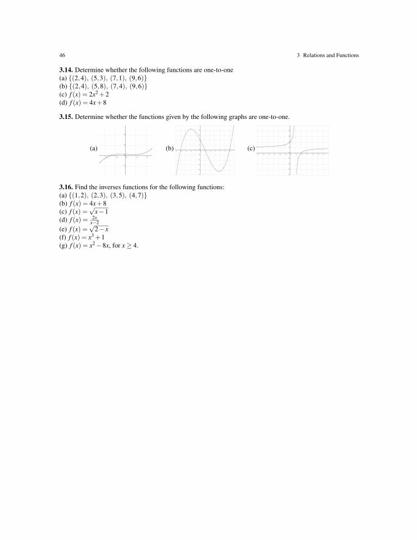
46 3 Relations and Functions
3.14. Determine whether the following functions are one-to-one(a) {(2,4), (5,3), (7,1), (9,6)}(b) {(2,4), (5,8), (7,4), (9,6)}(c) f (x) = 2x2 +2(d) f (x) = 4x+8
3.15. Determine whether the functions given by the following graphs are one-to-one.
(a) (b) (c)
3.16. Find the inverses functions for the following functions:(a) {(1,2), (2,3), (3,5), (4,7)}(b) f (x) = 4x+8(c) f (x) =
√x−1
(d) f (x) = 2xx−2
(e) f (x) =√
2− x(f) f (x) = x3 +1(g) f (x) = x2−8x, for x≥ 4.