adv anced insurance pla y in 21 : ris k av er sion and c om p osi...

Advanced Insurance Play in 21:Risk Aversion and Composition Dependence

R. Michael Canjar

Department of Mathematics and Computer Science, University of Detroit Mercy

Abstract. Risk-averse strategies for card counting in blackjack or twenty-one werefirst introduced in the landmark paper of Friedman (1980). These strategies arebased upon optimizing the player’s utility and/or reducing the player’s long-runindex (variance divided by square of expectation) rather than merely optimizing ex-pectation. This concept has now become part of mainstream blackjack theory andhas been endorsed in the popular literature (Schlesinger 2005). There are commer-cially available programs that will now compute risk-averse indices for all plays, withthe notable exception of the most important one, insurance. Risk-averse strategy forthis play necessarily involves the concept of partial insurance. This was presentedin Gri!n (1999) for the very important special case of insuring a natural.

This paper will give a comprehensive treatment of the theory of risk-averseinsurance. We will present and derive the pertinent mathematical equations andshow how to compute optimal partial insurance as well as insurance indices. Thisnecessarily involves the production of di"erent indices for di"erent hand totals, andthus requires a discussion of composition-dependent indices.

1 Introduction

In the game of blackjack (twenty-one), players are o!ered “insurance” when-ever the dealer’s up-card is an Ace. In most casinos, players may wager up tohalf their original bet, and this bet is paid o! at 2 to 1 if the casino holds aten-valued card under its Ace, giving it a natural. It is promoted as an op-portunity to “insure” a good hand. In reality, it usually functions as simplya side bet that the dealer’s hole card is a 10. (This paper will actually be anexception to that, in that here we will explore the “insurance” aspects of theinsurance wager.) Since approximately 4/13 of the cards in a full pack are10s, a simple calculation shows that the expectation on this bet is approx-imately 3(4/13) ! 1 = !1/13 = !7.6%, making it one of the worst wagersin the casino. Wagers like this are sometimes called “sucker bets.” However,a card-counting strategy is obvious: If more than 1/3 of the remaining cardsare 10s, then the wager has positive expectation for the player. This option is

4 R. Michael Canjar

quite valuable for a card counter, and all modern counting systems have anindex number for the insurance play. Indeed, this is the most important indexnumber in most systems.

Indices in counting systems have traditionally been based solely on maxi-mizing the player’s expectation. However, in recent years the more appropriateconcept of so-called “risk-averse” indices has become popular among blackjackplayers. This is a playing strategy based upon maximizing the player’s utility,and minimizing her long-run index: variance divided by expectation squared.The concept was originally introduced by Joel Friedman in his landmark paper(Friedman 1980), and now has become part of mainstream blackjack theory.It has recently been endorsed in the popular literature (Schlesinger 2005) andmost commercial simulators will now produce risk-averse index numbers forevery playing decision except insurance.

Insurance is inherently a di!erent and more complicated type of decisionbecause there is (negative) correlation between this bet and the other wagerthe player has made. Most players have an intuitive understanding that insur-ing a “good hand” reduces variance, and that these hands should be insuredat somewhat below the index. To some extent, the opposite is true for a weakhand. So the proper strategy will depend on the player’s holding. Also, riskaversion becomes more important with bigger bets, so a risk-averse insurancestrategy will depend on the size of our bets. We should note that our strategywill have more application to players who wager on two spots, as this willproduce larger optimal bets.

There was actually some preliminary discussion of this topic by Peter Grif-fin in his definitive book The Theory of Blackjack (1999). Gri"n computes thestrategy for insuring the best possible hand, a blackjack, that should be usedby a Kelly player, i.e., one using logarithmic utility. He shows that the optimalstrategy includes taking partial insurance under certain circumstances, whichwill be the key to our discussion. Gri"n’s solution is exact for this specialcase, but a more general treatment will require approximations.

My interest in this issue arose after Internet discussions with Steven Hestonin the early days of the bj21.com website. In particular, he pointed out to methe crucial role played by partial insurance and he helped to derive some ofthe formulas for pv below.

2 Risk-averse playing strategy

If advantage players simply wished to maximize their expectations, they wouldrisk their entire fortunes on each positive-expectation bet. Although there isan infinitesimal probability that such a player will become immensely wealthy,the overwhelming probability is that he/she will eventually go bankrupt. Thisis not usually regarded as a rational approach by responsible authors. In-stead, most texts on blackjack or advantage play advocate “optimal betting”strategies that seek to maximize a utility function. Such a function allows

Advanced Insurance Play in 21 5

quantification of the risk-reward tradeo!. For blackjack purposes, we can ap-proximate a wager’s certainty equivalent (CE) for reasonable utility functionswith the quadratic1

CE " EV ! 12

Vark Bank

, (1)

where EV is the expected value of the wager, Var is its variance, and Bank isthe size of the player’s bank, with EV,

#Var, and Bank measured in mone-

tary units (e.g., dollars). The parameter k is a constant that depends on theplayer’s utility function. It reflects the player’s risk aversion/risk tolerance.For logarithmic utility, k = 1. This utility gives rise to the famous “Kelly”betting system.

Note that to apply this formula we don’t need to know either the player’sBank or her risk aversion k, but only the product k Bank. This is sometimescalled the “Kelly-equivalent” bank.

Given a particular wagering opportunity, we can compute its mean µ andstandard deviation ! expressed as proportions of the amount wagered. !2 isthe variance, which we will denote by v. Let f be the amount wagered, ex-pressed as a fraction of the Kelly-equivalent bank. Then our certainty equiv-alent becomes

CE " k Bank!

µf ! vf2

2

"(2)

This function is maximized by selecting a betting fraction f = µ/v, which isthe basic equation for optimal betting. Note that optimal betting could becalled “risk-averse betting.”

Conventional playing strategy in blackjack simply looked at the expectedvalue of each decision and selected the one that was highest. Risk-averse strat-egy looks at the certainty equivalent of each decision and selects the one whoseCE is highest. It should really be called “optimal” playing strategy, if we usethat term in the same away that we do when we speak of “optimal betting.”

3 Underlying mathematics

Throughout the rest of the paper we will employ the following notation:

p The proportion of insurance that we take. Full insurance is wa-gering one-half of our bet on the insurance line and correspondsto p = 1. In most casinos, p is constrained to be between 0 and1.

d The density of 10-valued cards remaining in the pack.

µ The expectation of the insurance wager, namely 3d! 1.

1 A derivation of this formula is provided in Appendix 2.

6 R. Michael Canjar

R The result of the playing hand when the dealer has a natural.With standard rules, this is 0 if we have a blackjack and !1 forother hands.

CondEV The conditional expectation of the playing hand, computed un-der the assumption that the dealer does not have a BJ.

Suppose that we are in an insurance situation and we take partial insurancep. This partial insurance will a!ect both our expected value and our variance.We can compute this as a function of p, and then obtain our overall certaintyequivalent. Our CE will be a quadratic function of p, and it will obtain amaximum value for the optimal level insurance popt. After some mathematicalwork, the details of which are found in Appendix 1, we obtain the followingsimple and elegant formula for popt:

popt = p0 + pv, (3)

wherep0 =

29

#3d! 1

d(1! d)

$1f

=2µ

f(2 + µ! µ2)" µ

f, (4)

pv =23[!R + CondEV]. (5)

Each of these terms has a special significance, which we will elaborate onbelow. The first term, p0, represents the optimal insurance bet we would makein a stand-alone situation, where we did not have any money wagered on a BJhand. It tells us the amount we would bet if we had an opportunity to makean “over-the-shoulder” insurance bet on another player’s hand. The amountof this wager in monetary units does not depend on f ; its approximate valueis simply (µ/2)(k Bank). Eq. (4) expresses this insurance bet in terms of theamount of partial insurance to take on a hand with a blackjack wager of sizef · (k Bank). The pv term minimizes the overall variance of the result of ourinsurance bet and our playing hand.

Our formula for pv is exact. However we will use an approximation forp0. Our primary interest in risk-averse partial insurance will be when themagnitude of the expectation |µ| on the insurance wager is small. Otherwise wewill either not take insurance, or take as much insurance as we have available,depending on the algebraic sign of µ. Our simplification will be valid for smallvalues of µ.

Under ordinary blackjack rules, R is !1 except when the player has ablackjack. For these hands pv = (2/3)[1 + CondEV]. But if the player holdsa blackjack, R = 0 and CondEV = 3/2, in which case pv = 1, as we wouldexpect. We summarize:

pv =

%1 if player holds a blackjack,

(2/3)[1 + CondEV] if player holds any other hand.(6)


This applies for standard blackjack rules. If early surrender or Europeanhole card rules are applicable, then we would have to use a di!erent value forR.

4 Minimizing variance with pv

Let us consider the case where d = 1/3 and our insurance expectation is0. Whatever insurance wager we make will have no e!ect on our overall ex-pectation. It will a!ect our variance, and our optimal strategy is clearly tominimize the variance. We do that by taking p = pv specified above. Notethat the value of pv depends entirely on our playing hand. Strong hands thathave high CondEV will require higher insurance bets. Weak hands will requiresmaller insurance bets.

We estimated the CondEV for each possible playing hand. We put togetheran infinite pack that reflected the composition that a 10-counter would seeat the break-even point for insurance (d = 1/3). A combinatorial analysiswas performed over that pack. We assumed that the dealer stands on soft17. The values are listed in the Table A1 of the Appendix, along with thecorresponding values of pv.

Our formula calls for full insurance if we have a natural. This is obviouslycorrect for by doing so we guarantee that we make “even money” no matterwhat the dealer holds and we have reduced our variance to 0! But a blackjackis not the most insurable hand. The table shows that for a 20, we minimizevariance by taking 111% insurance. The reader may be surprised because 20is a weaker hand than 21. But with a blackjack, there is no possibility of aloss, and so there is less risk to avert.

As an exercise, the reader may wish to consider a variation on blackjack inwhich the house takes ties on blackjack. Then R = !1, and CondEV = 3/2,so our formula calls for (2/3)[1 + 3/2] = 140% of insurance, higher than thatfor a 20.

Of course, as a practical matter most casinos do not allow a player toover-insure, so if we held a 20, we would merely take the sub-optimal fullinsurance.

The reader may be surprised to see that even with a poor hand, somepartial insurance is called for. An easy example to look at is if the playerhas a hand that she wishes to surrender. Our formula calls for taking 1/3insurance. That is, if the player wagered 6 units, our formula calls for a 1-unitinsurance wager. Consider what happens. If the dealer has a BJ, we lose our6 units but make 2 units on insurance, for a net loss of 4 units. But if thedealer doesn’t have BJ, we lose 1 unit on the insurance and 3 units on thesurrender. Again the total loss is 4 units. We always lose the same 4 units;our variance has been reduced to 0.

This helps illustrate why we always take some insurance. Even a weakhand has some value. Insuring that small value reduces our variance.

8 R. Michael Canjar

It is customary for players who take full insurance on a blackjack to simplyrequest “even money.” If late surrender and partial insurance are both avail-able, the player could just as simply ask for the return of “one-third money”of the wager on poor hands, e!ectively o!ering to surrender two-thirds. Iwill refer to this maneuver as “modified early surrender” (MES) since it ismathematically equivalent to a type of surrender that could be done beforethe dealer checks for a blackjack. However, I would advise the reader againstthis, since it may indicate some mathematical understanding of the insurancebet, which is undesirable given the current state of paranoia among casinopersonnel.

For slot machines, it is customary to measure the expected value in termsof the amount of money returned by the machine. That is, a machine with EVof !3% is said to return 97%. This return is 1+CondEV. Note that this is theterm that is our formula for pv: It calls for us to insure 2/3 of the payback.

For another exercise, consider an unusual rule variation where a certainplayer hand is an automatic loser. That is, its CondEV = !1. This particularhand returns 0 and our formula yields pv = 0. This would be the extreme casein which we would have nothing to insure.

5 Rounding strategies and playing two hands

Of course, we cannot make exact insurance bets; we have to do some rounding.Our formula is based upon a quadratic approximation, and quadratics aresymmetric around their vertices. This means that “round to the nearest” willgive us the best possible result. For example, if an insurance bet of 1.3 unitsis optimal, it would be better to bet 1 unit rather than 2. But if 1.6 units wereoptimal, it would be better to wager 2 units.

What if the player can take only full insurance? If the choice is “all ornothing,” then our critical value is 50%. Take full insurance when p > 50%,and do not insure when p < 50%. We can set pv = 0.5 and solve to obtainCondEV = !25%. At the break-even point, we would insure hands whoseCondEV is above this value, and decline insurance for the others. From ourtable, this includes hard 8 and better hands. In particular, we do not take fullinsurance on a sti!. (To our knowledge, the first discussion of this strategywas by Peter Gri"n 1988.)

A corollary of this is that taking full insurance on a sti! hand actuallyincreases the overall variance.

Now what if the player is betting on two spots, and so has two hands inaction? We could treat these two hands as one entity with a certain aggregateCondEV and an aggregate R. Then we would plug these into our formulafor pv. However, CondEV is linear and R is linear (actually R is just theconditional expectation under the assumption that there is a dealer BJ) ourfinal result will just be the average of the pv values of the individual hands,weighted by bet size.


Here is an example. Suppose we bet 12 units on the left spot and 6 unitson the right. Inevitably, we get a blackjack on the right and a 16 on the left.Assume that we have a break-even situation for the insurance expectation.Our table tells us to take full insurance on the 6 unit bet (bet 3 units) , buttake 1/3 insurance on the 12 unit hand (bet 2 units). Our total insurance betshould be 5 units. We have taken 5/9 of our available insurance. This is theweighted average of 1/3 and 1, with the 1/3 weighted twice.

Examples like this have led most blackjack players to prefer wagers ofequal amounts when they are playing 2 spots. This is optimal for reducingvariance. If we are betting equal amounts, then we just do a simple average.

Even if the casino requires “all or nothing” insurance, we can insure onehand and not the other. E!ectively, this gives us half-insurance. If the decisionis “all, half, or none,” then our critical values are 25% and 75%. If less than25% of insurance is optimal, then we take no insurance. Between 25% and75%, we insure one of our two spots. Above that, we insure both.

Even a worse hand (16) calls for 30% insurance. If we have two such hands,our average is above 25%, so we should insure one of them. So we conclude:If we are playing two hands and we have a break-even insurance situation, wealways insure at least one of them.

If the hands are strong enough, we can take full insurance on both. Weneed the sum of their pv values to be 150%, so that the average is 75%. FromTable A1 in Appendix 2, we see that the following combinations are su"cientlystrong.

20 + hard 12 or better,BJ + hard 8 or better,19 + hard 9 (borderline) or better,

AA or 11 + hard 10 or better.

Of course, if partial insurance is allowed, there will be times where we takefull insurance on one spot and partial insurance on the other. Mathematically,it doesn’t matter which spot we put the full insurance on, but for the sake ofappearances, I recommend that you put the bigger insurance bet in front ofthe stronger hand.

Let me again emphasize that all of this discussion has been for the break-even case, µ = 0. In the next section, we discuss the more general situation.

6 The over-the-shoulder term p0

The other term in our formula is p0. While pv depends only on the hand weare playing, p0 depends on the insurance expectation and the size of our initialbet. The simplest way to understand p0 is to imagine this situation: Anotherplayer has wagered an amount f on a blackjack hand and is faced with aninsurance option. He/she doesn’t want to take it, but o!ers to allow you toexercise his/her option. What size insurance bet would you make?

10 R. Michael Canjar

Basically you would use your utility function and compute the “optimalbet” in a 2-to-1 wager game with expectation µ. If you used our quadraticapproximation, you would obtain a bet b = [µ/(2+µ!µ2)](k Bank). Now f =1/(k Bank). Also, p = 2b. Substituting these, we obtain p = 2µ/[(2+µ!µ2)f ],which was our original approximation for p0. Of course, we simplified thatfurther by approximating p " µ/f .

For a Kelly player who uses logarithmic utility, there is an exact solutionto this problem. The optimal bet for a wager that pays 2 : 1 is µBank /2.Translating this to our p and f notation gives our p = µ/f . That is, ourapproximation for p0 appears to be actually exact for the case of Kelly players.However, this is not completely accurate. While our methods give the correctvalue for the p0-term, as we have described it, they do not give the exactanswer for the overall value of popt. This is also discussed in Appendix 1.

The reader may be surprised that we simply add the p0 and pv termstogether to get our optimal bet. The next example may help to clarify that.

Example 1. Suppose that we hold a natural and the dealer has an Ace up. Wehave a large wager of f = 4% and our card-counting system estimates theinsurance expectation is !1%. pv = 100%, and our p0 = 1%/4% = !25%. Ifit were permitted, our optimal bet would be 1! 0.25 = 75% insurance. Thinkof this as a two-stage process. First we put out a 100% insurance bet. Thisis mathematically equivalent to settling the hand for “even money.” Now wehave essentially withdrawn the hand; mathematically it is as though we nolonger had any money on the betting square. But we have a negative-EV betin front of us, and our optimal bet on that would be to wager !25% of ourallowed insurance bet. Ordinarily casinos do not accept negative insurancebets, but here we can accomplish the same e!ect by pulling back some of themoney that we had planned to place on the insurance line.

Note that this is an example where risk-aversion causes us to make anegative-expectation insurance wager. It also helps to illustrate the relation-ship between optimal betting and risk-averse play. Declining “even-money” ona natural is essentially making a bet. The size of that bet should be computedproportionally, just like the size of any other bet. If the edge is marginal, wewould not make a “big bet”; that is, we would not completely decline the evenmoney.

Example 2. Suppose that we held a 16, and the insurance expectation is +1%.Since we plan to surrender the 16, our pv is 33 1

3%, and p0 is 25%. Our optimalplay would be 58% insurance. Again, think of two-stage betting. When we putout a 33 1

3% insurance bet, we are essentially settling for the return of one-third of our original wager, e!ectively surrendering two-thirds, which I earliercalled MES. We have removed all the variance from our playing hand, justas if we had no wager on the table. But again, we have a positive-EV bet infront of us on which we should make an optimal wager of p0.


If our only choice was all or nothing, then we would slightly prefer fullinsurance. But half-insurance would be better if permitted. Here is a casewhere we desire to take less than full insurance even though the insurance bethas positive expectation.

Example 3. Same as example 2, except that the insurance edge is only 0.5%.Then p0 become 12.5% and our optimal play is 46%. If our only choice is “allor nothing” insurance, then we would actually decline insurance, even thoughit is a positive-EV bet.

Our equations give us a linear relationship between p and µ. The playerwill usually measure µ via a count system, and our formulas give us p as alinear function of µ. However the typical constraint on p, 0 $ p $ 1, changesour function into a piecewise linear function, of the form

p =

&'(

')

0 if µ > µl,

µ/f + pv otherwise,1 if µ < µr,

(7)

as seen in the graphs in the Appendix.We can determine the left and right endpoints µl and µr by taking p = 0

and p = 1, respectively, in our equations

µ " [p! pv]f. (8)

Note that the length of the interval is proportional to the bet size f . Themidpoint of this interval (µ for p = 0.5) gives us the index for all-or-nothinginsurance. The quartiles (p = 0.25 and p = 0.75) give us the indices for half,all, or nothing. The interval will usually contain the conventional index, µ = 0.The exceptions are 20, where the conventional index lies to the right of theinterval, and blackjack, where it is the right endpoint.

We illustrate this by doing the computations for a 19 (pv = 80%) with abet size of 2%.

left endpoint: µl " (0! 0.8)2% = !1.6%right endpoint: µr " (1! 0.8)2% = 0.4%

“all or nothing” index: µ " (0.5! 0.8)2% = !0.6%“half or nothing” index: µ " (0.25! 0.8)2% = !1.1%

“half or all” index: µ " (0.75! 0.8)2% = !0.1%

Note that the length of the interval is 2%, the bet size.In the Appendix, we have included graphs that illustrate the typical partial

insurance interval. We have taken d, the density of 10s to be the independentvariable. Of course, d is just a linear function of µ, namely (µ + 1)/3.

The first graph is based upon a hard 18, pv " 0.6, with a 5% bet. Asan exercise the reader may verify that the interesting points have µ-valuesof !3.0%, !1.8%, !0.5%, 0.8%, 2.0%, and d-values of 32.3%, 32.8%, 33.2%,


33.6%, 34.0%. These are the points that correspond to the p-values of 0, 0.25,0.5, 0.75, 1.0.

Additional graphs are included to show the e!ects of hand-strength andbet size.

In practice, the player will employ a count system to estimate d and µ.This will be a linear functions of a parameter called the “true count.” Withthat linear function, we can transform these µ indices into count indices. Inthe next two sections, we will illustrate this with two popular count systems:the unbalanced 10-count and the Hi-Lo count.

7 Unbalanced 10-count

A 10-count gives a perfect estimation of insurance expectation µ. There area number of di!erent ways of counting 10s, but in our opinion the simplest isthe unbalanced ten count (UTC). In the UTC, we count 10s as !2, and allother cards as +1. We start with an initial running count of !4N , where Nis the number of decks used. In a 6-deck game, we would start at !24.

When the count is 0 (called the pivot point), insurance breaks even (µ =0). For positive counts, insurance has positive expectation, and for negativecounts it has negative expectation. Thus the conventional insurance playercan make decisions based simply on the algebraic sign of the UTC. A moresubtle feature of the UTC is that the insurance expectation µ is actually equalto its true count when measured in points per card. If instead we employ atrue count T of points per deck, then µ = T/52.

We can use this simple relationship to change the µ-indices described aboveinto T -indices, by simply taking T = 52µ. Let us illustrate this by revisitingthe example at the end of the previous section: a 19 with a bet size of 2%.

left-endpoint: µ " !1.6% so T -index is (!1.6%)(52) " !0.83right-endpoint: µ " 0.4% so T -index is (0.4%)(52) " 0.21

“all or nothing” index: µ " !0.6% so T -index is (!0.6%)(52) " !0.31“half or nothing” index: µ " !1.1% so T -index is (!.1.1%)(52) " !0.57

“half or all” index: µ " !0.1% so T -index is (!0.1%)(52) " !0.05

The length of our interval is (2%)(52) = 1.04 points per card. The shiftsin indices here will be very moderate and of very limited value. If we had abigger bet of 5% out, then the length of the interval would be 2.6 points percard, leading to some playable index shifts.

We have tabulated these indices for the 2% and 5% bet sizes in TablesA2 and A3 of the Appendix. These indices are based on playing one hand.However, if the player is wagering on two hands, he/she can simply take theweighted averages of the indices.

The table for 5% bets does give some interesting results for the “all, half,or full” insurance. This part is useful to players who have 2 spots and wish


to decide between insuring neither, one, or both spots. Note that for goodhands, the index for half-insurance is shifted 1–2. This means that the playershould buy some insurance, even though it is a negative-EV bet. Also, the“full insurance” index is shifted to the right for weak hands. If the player hastwo sti!s, he/she should not insure both of them until the true count is a fullpoint per deck over the index.

8 Another count system: Hi-Lo

While the 10-count is perfect for the insurance wager, it has a weak bettingcorrelation of 0.72. Other counts are usually used for betting purposes. Whilethere are players who have the remarkable ability to keep multiple countsand use them for di!erent purposes, most players keep only one count, anduse that count for all decisions. In this section we will show how they couldcompute our indices and discuss some of the other issues that occur.

Count systems typically determine a parameter called the “true count”T . A linear model may be used to relate deck composition, and thereforeinsurance expectation, to T . For insurance, our equation has the form:

µ " C(T ! Index0), (9)

where Index0 is the conventional insurance index, and C is a proportionalityconstant. We can solve this for T and substitute into the previous equation(8) to get our risk-averse index

RAIndex " Index0 +(p! pv)f

C. (10)

We plug in the critical values for p for the decision we are considering. For“all or nothing insurance,” we use p = 0.5.

One of the most popular count systems is the Hi-Lo. We will discuss it here,partly because it is so common, but also because it illustrates the problemsthat will occur with other count systems.

The Hi-Lo treats Aces and 10s as “high cards” and the player counts !1 foreach that is seen. Cards 2–6 are considered low and are counted +1. The 7, 8, 9are “neutral” and ignored (counted as 0). The player divides this “runningcount” by the number of unseen cards (or decks) to form a “true count.” Thistrue count gives a measure of deck composition and can be used to estimateexpectation for betting purposes and for playing decisions.

If we were playing from an infinite deck, we could compute our insuranceindex as follows. Let Tc be the true count in points per card. Let Td = 52Tc

be the points per deck. Tc may be increased by having a higher density of 10sand Aces, or a lower density of 2–6. We treat each of these as equally likely,so a representative pack with true count Tc has Tc/10 extra Aces, 10s, Js, Qs,Ks, and Tc/10 fewer 2s, 3s, 4s, 5s, 6s. Note that there are 10 ranks that are


counted, and four of these are 10-valued. Since the initial 10s density is 4/13,our 10s-density and insurance expectation are approximately

d " 413

+410

Tc, (11)

µ = 3d! 1 " ! 113

+1210

Tc " ! 113

+12520

Td " !7.60% + 2.30%Td. (12)

Setting µ = 0 gives us the infinite deck index Td = 10/3 " 3.33 which isthe “full pack” index for betting that the next card is a 10.

Thus when we compute Hi-Lo indices, we use a factor of 2.3% to translateexpectation into indices. The general formula is

RAIndex " Index0 +(p! pv)f

2.3%, (13)

where we plug in the critical value for p for the decision that we want, suchas 0.5 for “all-or-nothing insurance.”

Note that the length of the partial insurance interval is f/2.3%. See Table1.

Table 1. Length of Hi-Lo partial insurance interval.

bet size interval length

1% 0.42% 0.93% 1.34% 1.75% 2.26% 2.6

Fortunately for blackjack players, but unfortunately for blackjack analysts,blackjack is not dealt from an infinite deck. When we make a decision to insurea specific hand, we have some additional information that some specific cardshave been removed from the pack. That is, we can compute di!erent indicesfor each hand composition, which will be more accurate than a generic index.

For Hi-Lo, the known removal of Aces makes a big di!erence for our in-surance decisions. Hi-Lo does not distinguish between the Ace and the 10. Ifa number of Aces are removed, then insurance is more favorable, but Hi-Lothinks it is less favorable. We therefore adjust our Hi-Lo index to compensatefor this. Similar, but much smaller, e!ects exist for the other denominations.

Peter Gri"n appears to have been the first to have observed this phe-nomenon. Gri"n did a thorough computer analysis and determined exactvalues for all the single-deck compositions. He documented it in a private


letter to Prof. Edward Thorp on October 17, 1970. This was re-published inGri"n (1998) shortly after Gri"n’s death.

We will use a linear approximation to estimate the composition-dependentindices. Some of the mathematical justification for this will be included inAppendix 1. For each known removal, we will add or subtract an adjustmentto our insurance index. Table 2 shows the approximate adjustments.

Table 2. Adjustments to insurance index. (N is the number of decks.)

Ace !1.9/Nneutrals (7, 8, 9) !0.8/N10s +0.8/Nlows (2–6) +0.21/N

Let us illustrate this by computing the generic index for insuring a generichand for the various deck sizes. We add !1.9/N to adjust for the dealers Ace.See Table 3.

Table 3. Estimating generic Hi-Lo insurance indices.

single deck 3.3! 1.9/1 = 1.4double deck 3.3! 1.9/2 = 2.4six decks 3.3! 1.9/6 = 3.0

These are approximately the traditional indices used by Hi-Lo players.They are listed in Wong (1994, Table 11), where they are attributed toDr. Gri"n.

We have seen that risk-averse insurance depends on the specific hand weare playing, and in previous sections we have showed how to shift the conven-tional index to obtain risk-averse indices. However, each of the specific handshas a di!erent composition-dependent conventional index. For example, theconventional index for 10, 10 (Hard 20) can be estimated using the methodabove. For each 10 we add +0.8/N to the “generic indices” above, for a totalof 1.6/N . This gives the results in Table 4.

Note that we are working at cross-purposes to risk-aversion! Risk-aversionraises the index for 20 slightly, but the conventional index should be raised toadjust for the composition.

The situation can be di!erent for other hands. For example, if we have anAce and 9, the composition adjustment is (!1.9 ! 0.8)/N = !2.7/N , givingTable 5.


Table 4. Hi-Lo conventional insurance: 10, 10 vs. Ace.

single deck 1.4 + 1.6/1 = 3.0 (adjustment of + 1.6)double deck 2.4 + 1.6/2 = 3.2 (adjustment of + 0.8)six decks 3.3 + 1.6/6 = 3.6 (adjustment of + 0.3)

Table 5. Hi-Lo conventional insurance: Ace, 9 vs. Ace.

single deck 1.4! 2.7 = !1.3 (adjustment of ! 2.7)double deck 2.4! 2.7/2 = +1.1 (adjustment of ! 1.3)six decks 3.3 + 2.7/6 = +2.9 (adjustment of + 0.4)

The same phenomena will occur for other hands. For example, risk-aversionraises the index for 16. But the composition considerations raise the index for9, 7, although they do lower it for 10, 6.

We should also consider the orders of magnitude of these shifts. For modestsized bets of 2%, the entire partial insurance interval is less than 1 pointper deck. The shift in the index is less than that. But in single deck, thecomposition adjustments are typically greater and sometimes move in theopposite direction. The single-deck player who uses a lower index for insuring10, 10 will be making an error.

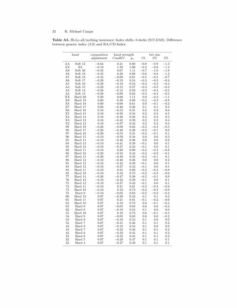
To illustrate this phenomenon, we have included tables for Hi-Lo insurancefor one- and six-deck games. Table A4 shows a single-deck game and TableA5 shows a six-deck one. We have also re-computed our estimates of the con-ditional expectation and the resulting pv parameter for these specific games,using rules more typical for them. For the single-deck game, we assumed thehouse hits soft 17 and for the six-deck game, we assumed that it stands on it.(In doing the computations for 8, 8, we assumed that double after split waspermitted in the six-deck game but not in the single-deck.) We have shownthe shifts in the indices for di!erent bet sizes, so that the reader can gaugethe order of magnitude of these e!ects.

9 Bet-sizing and practical considerations

As we have seen, optimal insurance involves a great deal of complexity. Thereare several parameters that go into each index, and there is a di!erent indexfor each play. Some simplifications are needed.

First, let us consider the issue of bet-sizing. We should assume that theplayer is using an “optimal” betting system, as it would be rather strange forsomeone to consider risk-aversion in insurance while ignoring it in betting!This in turn depends somewhat on the bet spread that the player uses. Usu-ally, players use a much smaller spread at single-deck than at multiple-deck.


At single-deck, bets rarely get over 1% or 2% of the Kelly-equivalent bank. Wesee that at these levels, risk-aversion is a minor factor. But composition de-pendence is a very important factor in single-deck. So for single-deck players,the composition-dependent e!ects are the most important.

For single-deck players that wish to use di!erent indices for various hands,I would recommend they focus on the composition dependence. Small RA-adjustments could be made for one representative bet size, such as 1%. I haveincluded a complete table of single-deck insurance indices for this level in TableA6 of the Appendix. These have indices for all our insurance decisions. At 1%,they are all fairly close to each other, and I would suggest that the player onlyuse one. (Single-deck players would do even better to just learn side-count,which would improve both their insurance decisions and their other playingdecisions as well.)

Wider spreads are often used in multiple-deck games. Total bets of 4% ofthe Kelly-equivalent bank are not that uncommon, particularly for someoneplaying two spots. In six-deck, the composition e!ects are minor, but at thisbet level the RA-e!ects are significant. To show this, I have included a tableof complete six-deck indices at the 4% bet level, as Table A7. Note that TablesA4/A5 show the shifts in indices, while Tables A6/A7 show the actual indices.

I would suggest that six-deck players start with the principle “When indoubt insure one of two spots.” They can refine the play by looking at our“half, all, or none” indices. Note that for the “good hands,” half insurance canbe taken as low as 2 when there is a big bet out. For poor hands, full-insurancecan be delayed until almost 4 when there is a big bet.

Again, if you are playing two spots, you simply average the indices foreach hand, weighting them by bet size.

Appendix 1. More mathematical details

In this appendix we will further elaborate on some of the details that wereomitted in the foregoing discussion.

A1.1 Optimizing the partial insurance

First, we will provide the derivation of our basic equations for the optimalpartial insurance bet. Our total result is the sum of two random variables.One is the result of the insurance wager, and the other is the original play-ing hand itself. We will temporarily call these Ins and Hand, respectively,and will let Tot = Ins +Hand be the sum of these. The bet on the in-surance wager is p/2 times the wager f on the hand. Note that E(Tot) =E(Ins) + E(Hand), whereas Var(Tot) = Var(Ins) + Var(Hand) + 2 Cov, whereCov is short for Cov(Ins,Hand). Our overall certainty equivalent is given byE(Tot)f ! Var(Tot)f2/2. If we express these in terms of the Ins and Handvariables, there will be five terms, two expectation terms, two variance terms,


and the covariance term. Now the E(Hand) and Var(Hand) terms are basi-cally just the certainty equivalent CE(Hand). If we write MCE(Ins) for themarginal certainty equivalent that the insurance bet adds, then we have

CE(Tot) = CE(Hand) + MCE(Ins), (14)

where

MCE(Ins) =!

pf

2

"E(Ins)! 1

2

!pf

2

"2

Var(Ins)! 12

2!

pf

2

"f Cov . (15)

Note that CE(Hand) is a constant term; its value does not depend on theamount p of partial insurance that we take. Essentially, this means that itis a “sunk cost,” which we can do nothing about. Note that the Var(Hand)only appears here, and so it has no e!ect on the optimal value of p in ourapproximation.

Our equation for MCE(Ins) is a quadratic in p, and we can rewrite it as

MCE(Ins) = "p! #p2, (16)

where

" =!

f

2

"E(Ins)!

!f2

2

"Cov, (17)

# =!

f2

8

"Var(Ins). (18)

Our quadratic will obtain a maximum at its vertex popt = "/(2#) or

popt = p0 + pv, (19)

where

p0 = 2E(Ins)

Var(Ins)1f

, (20)

pv = !2Cov

Var(Ins). (21)

Each of these terms has a special significance. The p0 term is exactlythe optimal insurance bet we would make if we considered insurance asa stand-alone bet, without reference to the hand. Our optimal bet bopt

would be [E(Ins)/ Var(Ins)]k Bank. Temporarily let bH be the amount thatwe have wagered on the hand, so that f = bH/(k Bank). Then k Bank =bH/f . Since a full insurance wager is bH/2, our optimal p will be 2b/bH =2[E(Ins)/ Var(Ins)]k Bank /bH = 2[E(Ins)/ Var(Ins)](bH/f)/bH , which is just(20).

Note also that pv minimizes the overall variance. If we wrote out theequation for the overall variance, it would contain the Var(Ins) and the Cov


term from the MCE(Ins) equation above, plus the Var(Hand) term. But theVar(Hand) term is just constant, and it will not a!ect the optimal value.

Let us compute the value of p0. Insurance is just a 2-to-1 bet with prob-ability d of success, so E(Ins) = µ = 3d ! 1 and Var(Ins) = 9d(1 ! d) or2 + µ! µ2. So this gives us

p0 =29

#3d! 1

d(1! d)

$1f

=2µ

f(2 + µ! µ2)" µ

f. (22)

For the pv term, we calculate the covariance. Consider a representation ofthe random variable Hand as a vector of possible outcomes %R,X1, X2, . . . , Xn&with corresponding probabilities %d, q1, q2, . . . , qn&. The vector for insurance is%2,!1,!1, . . . ,!1&. Note that

*q = 1! d and that CondEV =

*(qX)/(1!

d).Now the covariance is E(Ins · Hand)! E(Ins) · E(Hand) and

E(Ins · Hand) = d(2R) ++

(!1)qX = 2dR! (1! d) CondEV, (23)

E(Ins) · E(Hand) = µ · [dR + (1! d) CondEV]. (24)

Substituting in µ = 3d! 1 and simplifying we obtain

Cov = 3d(1! d)(R! CondEV), (25)

so that

pv = !2Cov

Var(Ins)= !2

3d(1! d)(R! CondEV)9d(1! d)

=23[!R + CondEV]. (26)

A1.2 Kelly digression: Do two wrongs make a right?

We used a quadratic approximation for CE. The “exact” solution that opti-mized this approximate function contained the p0-term of 2µ/[f(2 + µ!µ2)].We approximate this as µ/f . Now as pointed out above in the section on p0,this is exactly the amount of partial insurance that a Kelly player would takeon a stand-alone insurance bet. When I first considered this, it appeared thatour formula was exact for Kelly players. It looked as if two approximationscanceled each other, and that two wrongs made a right.

However, this is not quite true. While our methods give the correct valuefor the p0-term, as we have described it, they do not give the exact answerfor the overall value of popt.

A Kelly player uses logarithmic utility. For the case where there is novariance in the playing hand (such as when the player holds a blackjack orplans to surrender) we can actually compute the exact value of popt as

popt =µ

f+

23

[!R + CondEV] + µ

#R + 2 CondEV

3

$(27)


orpopt = p0 + pv + µ

#R + 2 CondEV

3

$. (28)

To derive this, let X1 = p+R be the amount of our gain if the house has anatural, and X2 = !p/2 + CondEV be our gain if it does not. A Kelly playerwishes to maximize his/her expected logarithm, which may be expressed

EL = d ln(1 + X1f) + (1! d) ln(1 + X2f)= d ln[1 + (p + R)f ] + (1! d) ln[1 + (!p/2 + CondEV)f ]. (29)

We wish to find the value of p that maximizes this. We take the derivative ofEL with respect to p obtaining

(EL)!(p) =df

1 + (p + R)f! 1

2(1! d)f

1 + (!p/2 + CondEV)f. (30)

We find the optimal p by setting this to 0 and solving. After simplifying theresult, we obtain the following:

popt =3d! 1

f+ 2d CondEV +(d! 1)R. (31)

This expresses popt in terms of d, but we would like to have it in terms ofµ = 3d!1. Note that d = (µ+1)/3. Our first term is simply µ/f . The secondterm becomes (2/3)(µ+1) CondEV, or µ(2/3) CondEV +(2/3) CondEV. Thefinal term becomes [(µ + 1)/3! 1]R or (µ/3)R! (2/3)R. If we group the twoµ-terms together, we simply obtain the last term in (27); if we group the otherterms together, we have pv.

The last term of (28) represents the error in our approximation. It is clearlyproportional to µ. For the case where the dealer holds a natural, the error isjust (1)µ; for the case of a surrender hand, the error is (!2/3)µ. The casewhere the player holds a blackjack is worked out in Gri"n (1999), where theexact answer is expressed in terms of the parameter that we are calling d, thedensity of 10s.

There is a simple explanation for this. Recall how we described the “two-step process” above. First, we take partial insurance pv to minimize variance.If we hold a natural, this means that we take “even money.” Then we takethe Kelly-optimal stand-alone insurance bet, µBank. We have approximatedBank as 1/f , but this is actually our pre-deal Bank. After we take “evenmoney,” our Bank has gone up by 1 bet, and is now 1/f + 1. Thus the Kellyoptimal bet is µ(1/f +1), as computed from (28). If we had a surrender hand,then our bank would go down by 2/3 of a bet when we execute an MES soour p0-term should really be (1)(1/f ! 2/3). Our quadratic approximation isnot clever enough to adjust for the change in our fortune.

This is a very general phenomenon, and it occurs with any utility function,provided the conditional payo!s to our blackjack hand are constant. To see


this, let U denote our utility, and let B denote our bank, measured in termsof the number of our current bets. (In other words, assume that our bet is 1unit). Let X1 = p + R be the amount of our gain if the house has a natural,and X2 = !p/2 + CondEV be our gain if it does not. Then our expectedutility is

EU = dU(B + X1) + (1! d)U(B + X2).= dU(B + p + R) + (1! d)U(B ! p/2 + CondEV). (32)

Let us introduce a new variable p! = p ! pv = p ! (2/3)[!R + CondEV].The optimal value of p! is the exact value of our p0.

Now if we accept “even-money” or “third-money” by taking pv partialinsurance, our expected result is [2 CondEV +R]/3. Call this amount EX.Note that

X1 ! EX = p + R! 13[2CondEV +R] = p! 2

3[!R + CondEV] = p!. (33)

And with a little more algebra,

X2 ! EX = !p

2+ CondEV!1

3[2CondEV +R]

= !12

#p! 2

3(CondEV!R)

$= !p!

2, (34)

so that our expected utility (32) becomes

EU = dU(B + EX1 + p!) + (1! d)U(B + EX ! p!/2). (35)

Let B! = B + EX. This our adjusted bank, after we accept “even money”or “early surrender two-thirds.” From (33), we see that B+X1 is B+EX+p! =B!+p!. From (34) we see that B+X2 = B+EX!p!/2 = B!!p!/2. Substitutingthese into (32) gives us

EU = dU(B! + p!) + (1! d)U(B! ! p!/2). (36)

This is precisely the same as our expected utility if we were making astand-alone insurance bet, of size p!, from our adjusted bank B!. The valueof p! that optimizes this will be precisely the optimal value of p0 as it wasdescribed earlier.

Of course, this relies heavily on the fact that our payo!s are constant.For most hands, they are not constant, and the exact solution would have anadditional term reflecting the conditional variance of our hand.

A1.3 Composition-dependent insurance

Here we will give a little more justification for the composition-dependentadjustments that were discussed above in the section on the Hi-Lo true count


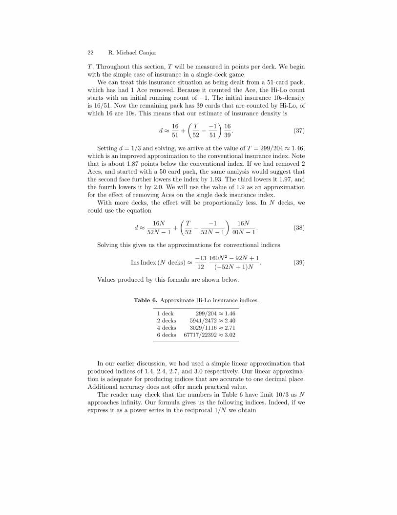
T . Throughout this section, T will be measured in points per deck. We beginwith the simple case of insurance in a single-deck game.

We can treat this insurance situation as being dealt from a 51-card pack,which has had 1 Ace removed. Because it counted the Ace, the Hi-Lo countstarts with an initial running count of !1. The initial insurance 10s-densityis 16/51. Now the remaining pack has 39 cards that are counted by Hi-Lo, ofwhich 16 are 10s. This means that our estimate of insurance density is

d " 1651

+!

T

52! !1

51

"1639

. (37)

Setting d = 1/3 and solving, we arrive at the value of T = 299/204 " 1.46,which is an improved approximation to the conventional insurance index. Notethat is about 1.87 points below the conventional index. If we had removed 2Aces, and started with a 50 card pack, the same analysis would suggest thatthe second face further lowers the index by 1.93. The third lowers it 1.97, andthe fourth lowers it by 2.0. We will use the value of 1.9 as an approximationfor the e!ect of removing Aces on the single deck insurance index.

With more decks, the e!ect will be proportionally less. In N decks, wecould use the equation

d " 16N

52N ! 1+

!T

52! !1

52N ! 1

"16N

40N ! 1. (38)

Solving this gives us the approximations for conventional indices

Ins Index (N decks) " !1312

160N2 ! 92N + 1(!52N + 1)N

. (39)

Values produced by this formula are shown below.

Table 6. Approximate Hi-Lo insurance indices.

1 deck 299/204 " 1.462 decks 5941/2472 " 2.404 decks 3029/1116 " 2.716 decks 67717/22392 " 3.02

In our earlier discussion, we had used a simple linear approximation thatproduced indices of 1.4, 2.4, 2.7, and 3.0 respectively. Our linear approxima-tion is adequate for producing indices that are accurate to one decimal place.Additional accuracy does not o!er much practical value.

The reader may check that the numbers in Table 6 have limit 10/3 as Napproaches infinity. Our formula gives us the following indices. Indeed, if weexpress it as a power series in the reciprocal 1/N we obtain


Ins Index (N decks) " 103! 289

156

!1N

"! 5

388

!1N

"2

(40)

or

Ins Index (N decks) " 103! (1.85)! (0.15)

!1N

"! (0.15)

!1N

"2

. (41)

We will further simplify this by approximating it as 10/3 ! 1.9/N . Note therole played by the number of decks N in computing our index.

There is a similar e!ect for removing the other cards tracked by Hi-Lo:the 10s, the lows, and the neutrals. In a similar way, the e!ect is roughlyproportional to the reciprocal of the number of decks. We will mercifullyspare the reader the details of obtaining the corresponding approximations.

Appendix 2. Derivation of CE equation

The concept of certainty equivalent arises from utility theory. We assume thata person has a utility function U(B), expressed in terms of wealth B. We willassume that U is a strictly increasing function. We will also see that theutilities that are of interest to advantage players are concave down. Given awager with payo!s of %X1, X2, . . .& per unit bet and corresponding probabili-ties %p1, p2, . . .& we can compute its expected utility EU =

*pkU(B + Xkb).

Here B is our wealth prior to the wager, and b is the bet size. The certaintyequivalent is the quantity CE that satisfies

U(B + CE) = EU =+

pkU(B + Xkb). (42)

That is, if we had a “wager” that paid us the amount CE with probability100%, then it would produce the same expected utility as EU . Equation (42)does define a function; since U is strictly increasing, it has an inverse U"1

and we could explicitly express CE as

CE = U"1(EU)!B = U"1,+

pkU(B + Xkb)-!B. (43)

However, I find it more convenient to work from (42). We will treat CE asa function CE(b) of the bet size b. As such, it has a second-order Taylorexpansion of the form

CE(b) = CE(0) + CE!(0)b +12

CE!!(0)b2 + O(b3). (44)

CE(0) is clearly 0, and we can find the derivatives CE! and CE!! from (42),using implicit di!erentiation. Taking the derivative of both sides gives us

U !(B + CE)CE! =+

pkU !(B + Xkb)Xk, (45)


from which we obtain

CE!(b) =+

pkU !(B + Xkb)Xk/U !(B + CE(b)). (46)

This gives us that CE!(0) =*

pkU !(B)Xk/U !(B) = µ. Taking the secondderivative with the quotient rule gives us

CE!!(b) =.+

pkU !!(B + Xkb)X2kU !(B + CE(b))

!+

pkU !(B + Xkb)XkU !!(B + CE(b))CE!(b)/

0[U !(B + CE(b))]2. (47)

Fortunately, this simplifies when we substitute in b = 0. Remembering thatCE(0) = 0, we have

CE!!(0) =.+

pkU !!(B)X2kU !(B)!

+pkU !(B)XkU !!(B) CE!(0)

/

0[U !(B)]2. (48)

Now*

pkX2k is the second moment M2 of our wager and

*pkXk is the mean

µ, and we know that CE!(0) = µ. Substituting, we have

CE!!(0) =U !!(B)U !(B)

(M2 ! µ2) =U !!(B)U !(B)

!2. (49)

For the utilities that interest us, U !!(B) < 0 and U !(B) > 0, so the coe"cientof !2 is negative. For some of the interesting utilities described below, themagnitude of this coe"cient is inversely proportional to B. This motivatesthe definition

k = !U !(B)/[BU !!(B)], (50)

which happens to be the reciprocal of the Arrow–Pratt measure of relativerisk aversion, so that our coe"cient of !2 is !1/(kB). Eq. (44) now becomes

CE = µb! !2

2kBb2 + O(b3). (51)

The first term µb is the expected value of the wager, and !2b2 is the variance.With slightly di!erent notation, we obtain eq. (1).

I conclude this section with the promised discussion of some specific util-ity functions. The Kelly betting system is associated with logarithmic utilityU(B) = lnB ; Kelly players seek to maximize the expected logarithm of thebankroll E[lnB]. For this utility, k = !U !/[BU !!] = !(B"1)/[B(!B"2)] = 1,as discussed in Section 1.

If we wished to determine the value of b that maximizes our CE, we couldapproximate this by finding where our quadratic approximation reaches amaximum. This occurs at the vertex:


bopt "µ

!2kB, (52)

which is the classical approximation for optimal betting.Another interesting utility function is U(B) = !B"1. For this utility,

k = !(B"2)/(!2B"3B) = 1/2. Players using this utility would thus bet halfof what a Kelly player would in any given situation; this is called half-Kellybetting. Here 1/2 is sometimes called the “Kelly fraction.” We can obtainutilities for any other Kelly fraction k ' (0, 1), by selecting U(W ) = !W p,where p = (k ! 1)/k.

At the beginning of this section I stated that the utilities of interest to ad-vantage players are concave down. For such utilities, our k will be positive, andthe coe"cient of !2 in (51) will be negative. Then even negative-expectationwagers would have positive CE. That is, such utilities would call for makingnegative-expectation wagers, which is not characteristic of advantage gam-blers.

Appendix 3. Graphs of partial insurance

The graphs illustrate the interval of partial insurance. The first example is amediocre hand (Hard 18) with big bet (f = 5%).

The length of the interval is proportional to the bet size f . The µ-lengthis f . The d-length is f/3. The Hi-Lo length is approximately f/2.3% Hi-Lopoints.

The conventional index (f = 0) occurs at d = 1/3. It is usually within theinterval. For weak hands, it is to the left of the interval. For strong hands, itis to the right of the interval. Exceptions: For BJ, the conventional index isthe right endpoint. For 20, the conventional index is outside the interval.

References

1. Friedman, J. F. (1980) Risk averse playing strategies in the game of blackjack.Presented at the Spring ORSA Conference, May.

2. Gri!n, Peter A. (1999) The Theory of Blackjack: The Compleat Card Counter’sGuide to the Casino Game of 21, 6th edition. Huntington Press, Las Vegas.

3. Gri!n, Peter (1988) Insure a good hand, part II. Blackjack Forum 8 (2).

4. Gri!n, Peter (1998) Letter to Edward Thorp, 16 Oct. 1970. Blackjack Forum 18(4).

5. Schlesinger, Don (2005) Blackjack Attack: Playing the Pros’ Way, 3rd edition.RGE Publishing, Las Vegas.

6. Wong, Stanford (1994) Professional Blackjack. Pi Yee Press.


0.31 0.32 0.33 0.34 0.35

0.0

0.2

0.4

0.6

0.8

1.0

1.2

–0.2

Index: Half or None

Index: All or Nothing

Index: All or Half

=0

Density of 10s

Pro

port

ion o

f In

sura

nce

Interval of Partial Insurance

Fig. 1. Graph for player 18.

0.31 0.32 0.33 0.34 0.35

0.0

0.2

0.4

0.6

0.8

1.0

1.2

–0.2

Index: Half or None


Index: All or Half

=0

Density of 10s

Pro

port

ion o

f In

sura

nce




0.31 0.32 0.33 0.34 0.35

0.0

0.2

0.4

0.6

0.8

1.0

1.2

–0.2

Index: Half or None


Index: All or Half

=0

Density of 10s

Pro

po

rtio

n o

f In

sura

nce


Fig. 3. Graph for player Surrender.

0.31 0.32 0.33 0.34 0.35

0.0

0.2

0.4

0.6

0.8

1.0

1.2

–0.2

Index: Half or None


Index: All or Half

=0

Density of 10s

Pro

po

rtio

n o

f In

sura

nce




Table A1. Minimizing variance with pv. Optimal partial insurance at the break-even point (µ = 0). Infinite deck; dealer stands on soft 17. Note: Conditional expec-tations were computed using an infinite deck, with additional 10s added to make10s-density equal 1/3.

hand action CondEV part. ins. pv ins. bet

Any 20 Stand 66% 111% 0.55

BJ Stand 150% 100% 0.50

Any 19 Stand 29% 86% 0.43

A, A Split 20% 80% 0.40

Hard 11 Double 20% 80% 0.40

Hard 10 Hit 10% 73% 0.37

Hard 9 Hit !5% 63% 0.32

Any 18 Stand !8% 61% 0.31

Soft 13 Hit !8% 61% 0.31

Soft 14 Hit !12% 59% 0.29

Soft 15 Hit !15% 56% 0.28

Soft 17 Hit !19% 54% 0.27

Soft 16 Hit !19% 54% 0.27

Hard 8 Hit !19% 54% 0.27

Hard 4 Hit !27% 49% 0.24

Hard 5 Hit !29% 47% 0.24

Hard 7 Hit !31% 46% 0.23

Hard 6 Hit !32% 45% 0.23

8, 8 Split !35% 43% 0.22

Hard 12 Hit !38% 42% 0.21

Hard 13 Hit !42% 39% 0.19

Hard 17 Stand !46% 36% 0.18

Hard 14 Hit !46% 36% 0.18

Hard 15 Hit !50% 34% 0.17

Hard 16 Surrender !50% 33% 0.17

Hard 16 Hit !53% 31% 0.16


Table A2. Risk-averse insurance interval and indices. Infinite deck; unbalanced 10count. Conventional index = 0. Bet size = 2%.

hand action hand strength interval indices

CondEV pv left right all/none half/none half/all

Any 20 Stand 66.30% 110.8% !1.15 !0.11 !0.63 !0.89 !0.37

BJ Stand 150.00% 100.0% !1.04 0.00 !0.52 !0.78 !0.26

Any 19 Stand 29.00% 86.0% !0.89 0.15 !0.37 !0.63 !0.11

A, A Split 20.20% 80.2% !0.83 0.21 !0.31 !0.57 !0.05

Hard 11 Dble 20.20% 80.2% !0.83 0.21 !0.31 !0.57 !0.05

Hard 10 Hit 10.20% 73.4% !0.76 0.28 !0.24 !0.50 0.02

Hard 9 Hit !5.00% 63.4% !0.66 0.38 !0.14 !0.40 0.12

Any 18 Stand !8.30% 61.2% !0.64 0.40 !0.12 !0.38 0.14

Soft 13 Hit !8.20% 61.2% !0.64 0.40 !0.12 !0.38 0.14

Soft 14 Hit !11.80% 58.8% !0.61 0.43 !0.09 !0.35 0.17

Soft 15 Hit !15.30% 56.4% !0.59 0.45 !0.07 !0.33 0.19

Soft 17 Hit !18.80% 54.2% !0.56 0.48 !0.04 !0.30 0.22

Soft 16 Hit !18.70% 54.2% !0.56 0.48 !0.04 !0.30 0.22

Hard 8 Hit !18.90% 54.0% !0.56 0.48 !0.04 !0.30 0.22

Hard 4 Hit !26.70% 48.8% !0.51 0.53 0.01 !0.25 0.27

Hard 5 Hit !29.20% 47.2% !0.49 0.55 0.03 !0.23 0.29

Hard 7 Hit !31.00% 46.0% !0.48 0.56 0.04 !0.22 0.30

Hard 6 Hit !31.80% 45.4% !0.47 0.57 0.05 !0.21 0.31

8, 8 Split !34.90% 43.4% !0.45 0.59 0.07 !0.19 0.33

Hard 12 Hit !37.50% 41.6% !0.43 0.61 0.09 !0.17 0.35

Hard 13 Hit !41.80% 38.8% !0.40 0.64 0.12 !0.14 0.38

Hard 17 Stand !45.60% 36.2% !0.38 0.66 0.14 !0.12 0.40

Hard 14 Hit !45.80% 36.2% !0.38 0.66 0.14 !0.12 0.40

Hard 15 Hit !49.60% 33.6% !0.35 0.69 0.17 !0.09 0.43

Hard 16 Surrender !50.00% 33.3% !0.35 0.69 0.17 !0.09 0.43

Hard 16 Hit !53.00% 31.4% !0.33 0.71 0.19 !0.07 0.45


Table A3. Risk-averse insurance interval and indices. Infinite deck; unbalanced 10count. Conventional index = 0. Bet size = 5%.

hand action hand strength interval indices

CondEV pv left right all/none half/none half/all

Any 20 Stand 66.30% 110.8% !2.88 !0.28 !1.58 !2.23 !0.93

BJ Stand 150.00% 100.0% !2.60 0.00 !1.30 !1.95 !0.65

Any 19 Stand 29.00% 86.0% !2.24 0.36 !0.94 !1.59 !0.29

A, A Split 20.20% 80.2% !2.09 0.51 !0.79 !1.44 !0.14

Hard 11 Dble 20.20% 80.2% !2.09 0.51 !0.79 !1.44 !0.14

Hard 10 Hit 10.20% 73.4% !1.91 0.69 !0.61 !1.26 0.04

Hard 9 Hit !5.00% 63.4% !1.65 0.95 !0.35 !1.00 0.30

Any 18 Stand !8.30% 61.2% !1.59 1.01 !0.29 !0.94 0.36

Soft 13 Hit !8.20% 61.2% !1.59 1.01 !0.29 !0.94 0.36

Soft 14 Hit !11.80% 58.8% !1.53 1.07 !0.23 !0.88 0.42

Soft 15 Hit !15.30% 56.4% !1.47 1.13 !0.17 !0.82 0.48

Soft 17 Hit !18.80% 54.2% !1.41 1.19 !0.11 !0.76 0.54

Soft 16 Hit !18.70% 54.2% !1.41 1.19 !0.11 !0.76 0.54

Hard 8 Hit !18.90% 54.0% !1.40 1.20 !0.10 !0.75 0.55

Hard 4 Hit !26.70% 48.8% !1.27 1.33 0.03 !0.62 0.68

Hard 5 Hit !29.20% 47.2% !1.23 1.37 0.07 !0.58 0.72

Hard 7 Hit !31.00% 46.0% !1.20 1.40 0.10 !0.55 0.75

Hard 6 Hit !31.80% 45.4% !1.18 1.42 0.12 !0.53 0.77

8, 8 Split !34.90% 43.4% !1.13 1.47 0.17 !0.48 0.82

Hard 12 Hit !37.50% 41.6% !1.08 1.52 0.22 !0.43 0.87

Hard 13 Hit !41.80% 38.8% !1.01 1.59 0.29 !0.36 0.94

Hard 17 Stand !45.60% 36.2% !0.94 1.66 0.36 !0.29 1.01

Hard 14 Hit !45.80% 36.2% !0.94 1.66 0.36 !0.29 1.01

Hard 15 Hit !49.60% 33.6% !0.87 1.73 0.43 !0.22 1.08

Hard 16 Surrender !50.00% 33.3% !0.87 1.73 0.43 !0.22 1.08

Hard 16 Hit !53.00% 31.4% !0.82 1.78 0.48 !0.17 1.13


Table A4. Hi-Lo all/nothing insurance: Index shifts. 1 deck (H17). Di"erence be-tween generic index (1.4) and RA/CD-Index.

hand composition hand strength bet sizeadjustment CondEV pv 1% 2% 5%

AA Soft 12 !3.84 0.236 0.824 !4.0 !4.1 !4.5AX BJ !1.15 1.500 1.000 !1.4 !1.6 !2.2A9 Soft 20 !2.71 0.636 1.091 !3.0 !3.2 !4.0A8 Soft 19 !2.71 0.205 0.803 !2.8 !3.0 !3.4A7 Soft 18 !2.71 !0.173 0.552 !2.7 !2.8 !2.8A6 Soft 17 !1.71 !0.238 0.508 !1.7 !1.7 !1.7A5 Soft 16 !1.71 !0.268 0.488 !1.7 !1.7 !1.7A4 Soft 15 !1.71 !0.185 0.543 !1.7 !1.7 !1.8A3 Soft 14 !1.71 !0.147 0.569 !1.7 !1.8 !1.9A2 Soft 13 !1.71 !0.091 0.606 !1.8 !1.8 !1.9XX Hard 20 1.54 0.602 1.068 1.3 1.0 0.3X9 Hard 19 !0.02 0.232 0.821 !0.2 !0.3 !0.7X8 Hard 18 !0.02 !0.184 0.544 0.0 !0.1 !0.1X7 Hard 17 !0.02 !0.476 0.349 0.0 0.1 0.3X6 Hard 16 0.98 !0.542 0.305 1.1 1.1 1.4X5 Hard 15 0.98 !0.537 0.308 1.1 1.1 1.4X4 Hard 14 0.98 !0.486 0.343 1.0 1.1 1.3X3 Hard 13 0.98 !0.440 0.373 1.0 1.1 1.3X2 Hard 12 0.98 !0.402 0.398 1.0 1.1 1.299 Hard 18 !1.58 !0.185 0.544 !1.6 !1.6 !1.798 Hard 17 !1.58 !0.483 0.345 !1.5 !1.4 !1.297 Hard 16 !1.58 !0.548 0.301 !1.5 !1.4 !1.196 Hard 15 !0.58 !0.518 0.321 !0.5 !0.4 !0.295 Hard 14 !0.58 !0.480 0.347 !0.5 !0.4 !0.294 Hard 13 !0.58 !0.399 0.400 !0.5 !0.5 !0.493 Hard 12 !0.58 !0.405 0.396 !0.5 !0.5 !0.492 Hard 11 !0.58 0.207 0.805 !0.7 !0.8 !1.288 Hard 16 !1.58 !0.473 0.352 !1.5 !1.5 !1.387 Hard 15 !1.58 !0.485 0.343 !1.5 !1.4 !1.286 Hard 14 !0.58 !0.487 0.342 !0.5 !0.4 !0.285 Hard 13 !0.58 !0.445 0.370 !0.5 !0.5 !0.384 Hard 12 !0.58 !0.403 0.398 !0.5 !0.5 !0.483 Hard 11 !0.58 0.226 0.817 !0.7 !0.9 !1.382 Hard 10 !0.58 0.041 0.694 !0.7 !0.7 !1.077 Hard 14 !1.58 !0.530 0.314 !1.5 !1.4 !1.276 Hard 13 !0.58 !0.451 0.366 !0.5 !0.5 !0.375 Hard 12 !0.58 !0.408 0.395 !0.5 !0.5 !0.474 Hard 11 !0.58 0.245 0.830 !0.7 !0.9 !1.373 Hard 10 !0.58 0.040 0.694 !0.7 !0.7 !1.072 Hard 9 !0.58 !0.133 0.578 !0.6 !0.6 !0.766 Hard 12 0.42 !0.405 0.396 0.5 0.5 0.665 Hard 11 0.42 0.252 0.834 0.3 0.1 !0.364 Hard 10 0.42 0.046 0.698 0.3 0.2 0.063 Hard 9 0.42 !0.119 0.587 0.4 0.3 0.262 Hard 8 0.42 !0.278 0.482 0.4 0.4 0.555 Hard 10 0.42 0.042 0.695 0.3 0.3 0.054 Hard 9 0.42 !0.120 0.587 0.4 0.3 0.253 Hard 8 0.42 !0.281 0.479 0.4 0.4 0.552 Hard 7 0.42 !0.368 0.422 0.5 0.5 0.644 Hard 8 0.42 !0.269 0.487 0.4 0.4 0.443 Hard 7 0.42 !0.377 0.415 0.5 0.5 0.642 Hard 6 0.42 !0.378 0.414 0.5 0.5 0.633 Hard 6 0.42 !0.379 0.414 0.5 0.5 0.632 Hard 5 0.42 !0.323 0.451 0.4 0.5 0.522 Hard 4 0.42 !0.298 0.468 0.4 0.4 0.5


Table A5. Hi-Lo all/nothing insurance: Index shifts. 6 decks (S17-DAS). Di"erencebetween generic index (3.0) and RA/CD-Index.

hand composition hand strength bet sizeadjustment CondEV pv 1% 2% 5%

AA Soft 12 !0.64 0.21 0.80 !0.8 !0.9 !1.3AX BJ !0.19 1.50 1.00 !0.4 !0.6 !1.3A9 Soft 20 !0.45 0.67 1.11 !0.7 !1.0 !1.8A8 Soft 19 !0.45 0.29 0.86 !0.6 !0.8 !1.2A7 Soft 18 !0.45 !0.09 0.61 !0.5 !0.5 !0.7A6 Soft 17 !0.28 !0.19 0.54 !0.3 !0.3 !0.4A5 Soft 16 !0.28 !0.19 0.54 !0.3 !0.3 !0.4A4 Soft 15 !0.28 !0.15 0.57 !0.3 !0.3 !0.4A3 Soft 14 !0.28 !0.12 0.59 !0.3 !0.4 !0.5A2 Soft 13 !0.28 !0.08 0.62 !0.3 !0.4 !0.5XX Hard 20 0.26 0.66 1.11 0.0 !0.3 !1.1X9 Hard 19 0.00 0.30 0.86 !0.2 !0.3 !0.8X8 Hard 18 0.00 !0.08 0.61 0.0 !0.1 !0.2X7 Hard 17 0.00 !0.46 0.36 0.1 0.1 0.3X6 Hard 16 0.16 !0.53 0.31 0.2 0.3 0.6X5 Hard 15 0.16 !0.50 0.34 0.2 0.3 0.5X4 Hard 14 0.16 !0.46 0.36 0.2 0.3 0.5X3 Hard 13 0.16 !0.42 0.39 0.2 0.3 0.4X2 Hard 12 0.16 !0.37 0.42 0.2 0.2 0.399 Hard 18 !0.26 !0.08 0.62 !0.3 !0.4 !0.598 Hard 17 !0.26 !0.46 0.36 !0.2 !0.1 0.097 Hard 16 !0.26 !0.53 0.31 !0.2 !0.1 0.196 Hard 15 !0.10 !0.50 0.34 0.0 0.0 0.395 Hard 14 !0.10 !0.46 0.36 0.0 0.0 0.294 Hard 13 !0.10 !0.41 0.39 !0.1 0.0 0.193 Hard 12 !0.10 !0.37 0.42 !0.1 0.0 0.192 Hard 11 !0.10 0.20 0.80 !0.2 !0.4 !0.888 Hard 16 !0.26 !0.34 0.44 !0.2 !0.2 !0.187 Hard 15 !0.26 !0.49 0.34 !0.2 !0.1 0.186 Hard 14 !0.10 !0.46 0.36 0.0 0.0 0.285 Hard 13 !0.10 !0.42 0.39 !0.1 0.0 0.184 Hard 12 !0.10 !0.37 0.42 !0.1 0.0 0.183 Hard 11 !0.10 0.21 0.80 !0.2 !0.4 !0.882 Hard 10 !0.10 0.10 0.73 !0.2 !0.3 !0.677 Hard 14 !0.26 !0.47 0.36 !0.2 !0.1 0.076 Hard 13 !0.10 !0.42 0.39 !0.1 0.0 0.175 Hard 12 !0.10 !0.37 0.42 !0.1 0.0 0.174 Hard 11 !0.10 0.21 0.81 !0.2 !0.4 !0.873 Hard 10 !0.10 0.10 0.73 !0.2 !0.3 !0.672 Hard 9 !0.10 !0.05 0.63 !0.2 !0.2 !0.466 Hard 12 0.07 !0.38 0.42 0.1 0.1 0.265 Hard 11 0.07 0.21 0.81 !0.1 !0.2 !0.664 Hard 10 0.07 0.10 0.73 0.0 !0.1 !0.463 Hard 9 0.07 !0.05 0.63 0.0 0.0 !0.262 Hard 8 0.07 !0.19 0.54 0.1 0.0 0.055 Hard 10 0.07 0.10 0.73 0.0 !0.1 !0.454 Hard 9 0.07 !0.05 0.63 0.0 0.0 !0.253 Hard 8 0.07 !0.19 0.54 0.1 0.0 0.052 Hard 7 0.07 !0.31 0.46 0.1 0.1 0.244 Hard 8 0.07 !0.19 0.54 0.1 0.0 0.043 Hard 7 0.07 !0.32 0.46 0.1 0.1 0.242 Hard 6 0.07 !0.32 0.45 0.1 0.1 0.233 Hard 6 0.07 !0.32 0.45 0.1 0.1 0.232 Hard 5 0.07 !0.29 0.47 0.1 0.1 0.122 Hard 4 0.07 !0.27 0.49 0.1 0.1 0.1


Table A6. Complete Hi-Lo single-deck insurance indices. Bet size: 1%. Rules: H17.

hand composition hand strength interval indicesadjustment CondEV pv left right all/none half/none half/all

AA Pair Aces !3.8 0.24 0.8 !2.8 !2.3 !2.5 !2.7 !2.4AX BJ !1.2 1.50 1.0 !0.2 0.3 0.1 0.0 0.2A9 Soft 20 !2.7 0.64 1.1 !1.8 !1.3 !1.5 !1.6 !1.4A8 Soft 19 !2.7 0.21 0.8 !1.6 !1.2 !1.4 !1.5 !1.3A7 Soft 18 !2.7 !0.17 0.6 !1.5 !1.1 !1.3 !1.4 !1.2A6 Soft 17 !1.7 !0.24 0.5 !0.5 !0.1 !0.3 !0.4 !0.2A5 Soft 16 !1.7 !0.27 0.5 !0.5 !0.1 !0.3 !0.4 !0.2A4 Soft 15 !1.7 !0.19 0.5 !0.5 !0.1 !0.3 !0.4 !0.2A3 Soft 14 !1.7 !0.15 0.6 !0.5 !0.1 !0.3 !0.4 !0.2A2 Soft 13 !1.7 !0.09 0.6 !0.5 !0.1 !0.3 !0.4 !0.2XX Hard 20 1.5 0.60 1.1 2.5 2.9 2.7 2.6 2.8X9 Hard 19 0.0 0.23 0.8 1.1 1.5 1.3 1.2 1.4X8 Hard 18 0.0 !0.18 0.5 1.2 1.6 1.4 1.3 1.5X7 Hard 17 0.0 !0.48 0.3 1.3 1.7 1.5 1.4 1.6X6 Hard 16 1.0 !0.54 0.3 2.3 2.7 2.5 2.4 2.6X5 Hard 15 1.0 !0.54 0.3 2.3 2.7 2.5 2.4 2.6X4 Hard 14 1.0 !0.49 0.3 2.3 2.7 2.5 2.4 2.6X3 Hard 13 1.0 !0.44 0.4 2.3 2.7 2.5 2.4 2.6X2 Hard 12 1.0 !0.40 0.4 2.2 2.7 2.5 2.3 2.699 Hard 18 !1.6 !0.19 0.5 !0.4 0.1 !0.2 !0.3 !0.198 Hard 17 !1.6 !0.48 0.3 !0.3 0.1 !0.1 !0.2 0.097 Hard 16 !1.6 !0.55 0.3 !0.3 0.2 !0.1 !0.2 0.096 Hard 15 !0.6 !0.52 0.3 0.7 1.1 0.9 0.8 1.095 Hard 14 !0.6 !0.48 0.3 0.7 1.1 0.9 0.8 1.094 Hard 13 !0.6 !0.40 0.4 0.7 1.1 0.9 0.8 1.093 Hard 12 !0.6 !0.41 0.4 0.7 1.1 0.9 0.8 1.092 Hard 11 !0.6 0.21 0.8 0.5 0.9 0.7 0.6 0.888 Pair 8s !1.6 !0.47 0.4 !0.3 0.1 !0.1 !0.2 0.087 Hard 15 !1.6 !0.49 0.3 !0.3 0.1 !0.1 !0.2 0.086 Hard 14 !0.6 !0.49 0.3 0.7 1.1 0.9 0.8 1.085 Hard 13 !0.6 !0.45 0.4 0.7 1.1 0.9 0.8 1.084 Hard 12 !0.6 !0.40 0.4 0.7 1.1 0.9 0.8 1.083 Hard 11 !0.6 0.23 0.8 0.5 0.9 0.7 0.6 0.882 Hard 10 !0.6 0.04 0.7 0.6 1.0 0.8 0.7 0.977 Hard 14 !1.6 !0.53 0.3 !0.3 0.2 !0.1 !0.2 0.076 Hard 13 !0.6 !0.45 0.4 0.7 1.1 0.9 0.8 1.075 Hard 12 !0.6 !0.41 0.4 0.7 1.1 0.9 0.8 1.074 Hard 11 !0.6 0.25 0.8 0.5 0.9 0.7 0.6 0.873 Hard 10 !0.6 0.04 0.7 0.6 1.0 0.8 0.7 0.972 Hard 9 !0.6 !0.13 0.6 0.6 1.0 0.8 0.7 0.966 Hard 12 0.4 !0.41 0.4 1.7 2.1 1.9 1.8 2.065 Hard 11 0.4 0.25 0.8 1.5 1.9 1.7 1.6 1.864 Hard 10 0.4 0.05 0.7 1.5 2.0 1.8 1.7 1.963 Hard 9 0.4 !0.12 0.6 1.6 2.0 1.8 1.7 1.962 Hard 8 0.4 !0.28 0.5 1.6 2.1 1.9 1.8 2.055 Hard 10 0.4 0.04 0.7 1.6 2.0 1.8 1.7 1.954 Hard 9 0.4 !0.12 0.6 1.6 2.0 1.8 1.7 1.953 Hard 8 0.4 !0.28 0.5 1.6 2.1 1.9 1.8 2.052 Hard 7 0.4 !0.37 0.4 1.7 2.1 1.9 1.8 2.044 Hard 8 0.4 !0.27 0.5 1.6 2.1 1.9 1.8 2.043 Hard 7 0.4 !0.38 0.4 1.7 2.1 1.9 1.8 2.042 Hard 6 0.4 !0.38 0.4 1.7 2.1 1.9 1.8 2.033 Hard 6 0.4 !0.38 0.4 1.7 2.1 1.9 1.8 2.032 Hard 5 0.4 !0.32 0.5 1.7 2.1 1.9 1.8 2.022 Hard 4 0.4 !0.30 0.5 1.6 2.1 1.9 1.8 2.0


Table A7. Complete Hi-Lo six-deck insurance indices. Bet size: 4%. Rules: S17DAS.

hand composition hand strength interval indicesadjustment CondEV pv left right all/none half/none half/all

AA Pair Aces !0.64 0.21 0.80 1.0 2.7 1.8 1.4 2.3AX BJ !0.19 1.50 1.00 1.1 2.8 2.0 1.5 2.4A9 Soft 20 !0.45 0.67 1.11 0.6 2.4 1.5 1.1 1.9A8 Soft 19 !0.45 0.29 0.86 1.1 2.8 1.9 1.5 2.4A7 Soft 18 !0.45 !0.09 0.61 1.5 3.2 2.4 1.9 2.8A6 Soft 17 !0.28 !0.19 0.54 1.8 3.5 2.7 2.2 3.1A5 Soft 16 !0.28 !0.19 0.54 1.8 3.5 2.7 2.2 3.1A4 Soft 15 !0.28 !0.15 0.57 1.8 3.5 2.6 2.2 3.1A3 Soft 14 !0.28 !0.12 0.59 1.7 3.5 2.6 2.1 3.0A2 Soft 13 !0.28 !0.08 0.62 1.7 3.4 2.5 2.1 3.0XX Hard 20 0.26 0.66 1.11 1.4 3.1 2.2 1.8 2.7X9 Hard 19 0.00 0.30 0.86 1.5 3.3 2.4 2.0 2.8X8 Hard 18 0.00 !0.08 0.61 2.0 3.7 2.8 2.4 3.3X7 Hard 17 0.00 !0.46 0.36 2.4 4.1 3.3 2.8 3.7X6 Hard 16 0.16 !0.53 0.31 2.6 4.4 3.5 3.1 3.9X5 Hard 15 0.16 !0.50 0.34 2.6 4.3 3.5 3.0 3.9X4 Hard 14 0.16 !0.46 0.36 2.5 4.3 3.4 3.0 3.9X3 Hard 13 0.16 !0.42 0.39 2.5 4.2 3.4 2.9 3.8X2 Hard 12 0.16 !0.37 0.42 2.4 4.2 3.3 2.9 3.899 Hard 18 !0.26 !0.08 0.62 1.7 3.4 2.6 2.1 3.098 Hard 17 !0.26 !0.46 0.36 2.1 3.9 3.0 2.6 3.497 Hard 16 !0.26 !0.53 0.31 2.2 3.9 3.1 2.6 3.596 Hard 15 !0.10 !0.50 0.34 2.3 4.1 3.2 2.8 3.695 Hard 14 !0.10 !0.46 0.36 2.3 4.0 3.2 2.7 3.694 Hard 13 !0.10 !0.41 0.39 2.2 4.0 3.1 2.7 3.593 Hard 12 !0.10 !0.37 0.42 2.2 3.9 3.1 2.6 3.592 Hard 11 !0.10 0.20 0.80 1.5 3.3 2.4 2.0 2.888 Pair 8s !0.26 !0.34 0.44 2.0 3.7 2.9 2.4 3.387 Hard 15 !0.26 !0.49 0.34 2.2 3.9 3.0 2.6 3.586 Hard 14 !0.10 !0.46 0.36 2.3 4.0 3.2 2.7 3.685 Hard 13 !0.10 !0.42 0.39 2.2 4.0 3.1 2.7 3.584 Hard 12 !0.10 !0.37 0.42 2.2 3.9 3.1 2.6 3.583 Hard 11 !0.10 0.21 0.80 1.5 3.3 2.4 2.0 2.882 Hard 10 !0.10 0.10 0.73 1.6 3.4 2.5 2.1 2.977 Hard 14 !0.26 !0.47 0.36 2.1 3.9 3.0 2.6 3.476 Hard 13 !0.10 !0.42 0.39 2.2 4.0 3.1 2.7 3.575 Hard 12 !0.10 !0.37 0.42 2.2 3.9 3.1 2.6 3.574 Hard 11 !0.10 0.21 0.81 1.5 3.3 2.4 2.0 2.873 Hard 10 !0.10 0.10 0.73 1.6 3.4 2.5 2.1 2.972 Hard 9 !0.10 !0.05 0.63 1.8 3.6 2.7 2.3 3.166 Hard 12 0.07 !0.38 0.42 2.4 4.1 3.2 2.8 3.765 Hard 11 0.07 0.21 0.81 1.7 3.4 2.6 2.1 3.064 Hard 10 0.07 0.10 0.73 1.8 3.6 2.7 2.2 3.163 Hard 9 0.07 !0.05 0.63 2.0 3.7 2.9 2.4 3.362 Hard 8 0.07 !0.19 0.54 2.2 3.9 3.0 2.6 3.555 Hard 10 0.07 0.10 0.73 1.8 3.6 2.7 2.2 3.154 Hard 9 0.07 !0.05 0.63 2.0 3.7 2.9 2.4 3.353 Hard 8 0.07 !0.19 0.54 2.2 3.9 3.0 2.6 3.552 Hard 7 0.07 !0.31 0.46 2.3 4.0 3.2 2.7 3.644 Hard 8 0.07 !0.19 0.54 2.1 3.9 3.0 2.6 3.543 Hard 7 0.07 !0.32 0.46 2.3 4.0 3.2 2.7 3.642 Hard 6 0.07 !0.32 0.45 2.3 4.0 3.2 2.7 3.633 Hard 6 0.07 !0.32 0.45 2.3 4.0 3.2 2.7 3.632 Hard 5 0.07 !0.29 0.47 2.3 4.0 3.1 2.7 3.622 Hard 4 0.07 !0.27 0.49 2.2 4.0 3.1 2.7 3.5

adv anced insurance pla y in 21 : ris k av er sion and c om p osi...

Documents