additional crossing of the clarence river at grafton · preferred location for an additional...
TRANSCRIPT

Route Options Development Report Technical Paper – Economic Evaluation
SEPTEMBER 2012
Additional crossing of the Clarence River at Grafton

whatwouldyouliketogrow.com.au
AdditionalCrossing of theClarence River atGraftonRoute Options DevelopmentReport
Technical Paper - EconomicEvaluation
Final
Arup
August 2012

Disclaimer
This Report has been prepared by PricewaterhouseCoopers (PwC) at the request of theArup, to conduct an economic evaluation (EE) of an additional crossing of the ClarenceRiver at Grafton.
The information, statements, statistics and commentary (together the “Information”)contained in this Report have been prepared by PwC from material provided by Arup, itstechnical advisers and from other industry data from sources external to Arup. PwC mayat its absolute discretion, but without being under any obligation to do so, update, amendor supplement this document.
PwC does not express an opinion as to the accuracy or completeness of the informationprovided, the assumptions made by the parties that provided the information or anyconclusions reached by those parties. PwC disclaims any and all liability arising fromactions taken in response to this report. PwC disclaims any and all liability for anyinvestment or strategic decisions made as a consequence of information contained in thisreport. PwC, its employees and any persons associated with the preparation of theenclosed documents are in no way responsible for any errors or omissions in the encloseddocument resulting from any inaccuracy, mis-description or incompleteness of theinformation provided or from assumptions made or opinions reached by the parties thatprovided information.
PwC has based this Report on information received or obtained, on the basis that suchinformation is accurate and, where it is represented by Arup as such, complete. TheInformation contained in this report has not been subject to an Audit. The informationmust not be copied, reproduced, distributed, or used, in whole or in part, for any purposeother than detailed in our Consultant Agreement without the written permission of theArup and PwC.
Comments and queries can be directed to:
Scott LennonPartner – PricewaterhouseCoopersPh: (02) 8266 2765Email: [email protected]


ArupPwC i What would you like to grow?
Contents
Executive Summary 2
Glossary 5
1 Introduction 8
2 Rationale for an additional crossing of the Clarence River 11
3 Economic evaluation methodology 28
4 Demand (traffic) analysis 32
5 Estimating road user and external costs 43
6 Direct infrastructure costs 53
7 Results 60
8 Conclusions 64
Appendix A Grafton Bridge 66
Appendix B Traffic modelling study area 67
Appendix C Unadjusted capital cost estimates 68
Appendix D Capital cost cashflows by route option 74
Appendix E Detailed road user and external cost profiles 80
Executive Summary
2 What would you like to grow?
Executive Summary
Background
Roads and Maritime Services (RMS, formerly RTA) is currently undertaking investigations to identify thepreferred location for an additional crossing of the Clarence River at Grafton to address short-term and long-term transport needs. Arup (on behalf of RMS) has engaged PricewaterhouseCoopers (PwC) to undertake aneconomic evaluation of six short-listed route options. This technical paper builds on the work undertaken forthe Preliminary Route Options Report Final (PROR) and is an attachment to the Route Options DevelopmentReport. This Economic Evaluation (EE) is primarily concerned with transport related outcomes. RMS willdetermine the recommended route option based on its performance against a wider range of indicators (i.e.environment, amenity, heritage etc.). Information on non-transport indicators will be provided by othertechnical streams.
Transport issues in the study area
While Grafton and South Grafton have respective residential and employment centres, forecast significantgrowth in population is expected to add to the existing focus on residential land uses in South Grafton. Thiswill increase demand for trips crossing the river to access employment and services concentrated in Grafton.Population growth in the Grafton area is expected to increase the demand for bridge crossings by 108 per centover the next 30 years.
Negative social, environmental and economic outcomes occur when the capacity and design of the existingtransport network cannot accommodate the growth in the number of trips. The key transport problems in theGrafton area relate to:
the insufficient capacity of the existing bridge;
sub-optimal alignment and design of the existing bridge;
the reliance on the bridge evidenced by the high proportion of total network trips which involve ariver crossing; and
the lack of practical alternative routes crossing the river.
Route options
RMS seeks to address the transport problems above through a short-list of six route options. These are shownbelow in Table ES 1. A graphical presentation of the route option alignment follows in Figure ES 1.
Table ES 1: Short-listed route options
RouteOption
Description
E Option E includes a new bridge upstream of the existing bridge where it would connect theGwydir Highway at Cowan Street in South Grafton to Villiers Street in Grafton. Both thenew and existing bridge would have one lane in each direction.
A Option A consists of a new bridge constructed slightly upstream and parallel to the existingbridge. This option would connect Bent Street in South Grafton to Fitzroy Street inGrafton. The new bridge would have two northbound lanes and one southbound lane andthe existing bridge will be converted to one southbound lane.
C Option C involves building a new bridge slightly downstream and parallel to the existingbridge. This option connects the Pacific Highway at Iolanthe Street in South Grafton toClarence and Pound Street in Grafton. Under Option C, both bridges would have one lanein each direction.
11 Option 11 involves the construction of a new bridge downstream of the existing bridgewhere it would connect the Pacific Highway at McClaers Lane in South Grafton to Fry Streetin Grafton. Option 11 would include two viaduct structures between the Pacific Highwayand the Clarence River. It would also include an upgrade of Fry Street to enable it to meet

Executive Summary
ArupPwC 3 What would you like to grow?
RouteOption
Description
future traffic volumes and of Villiers Street to accommodate a 5.3m vertical clearance forheavy vehicles beneath the railway viaduct. Both bridges would have one lane in eachdirection.
14 Option 14 involves the construction of a new bridge downstream of the existing bridgewhere it connects Pacific Highway at Centenary Drive in South Grafton and North Street viaKirchner Street at Grafton. Both the new and existing bridge would be one lane in eachdirection.
15 Option 15 involves the construction of a new bridge downstream of the existing bridgewhere it connects Pacific Highway at Centenary Drive in South Grafton to SummerlandWay via Kirchner Street in Grafton. All construction aspects are the same as Option 14; theonly difference is the alignment of the connections on the Grafton side.
Figure ES 1: Short-listed route options
Approach to economic evaluation
The economic evaluation of the six route options is undertaken using Cost Benefit Analysis (CBA). CBAmeasures the economic viability of a route option by comparing the additional benefits of the route option withthe additional costs with a route option, over a defined evaluation period. The additional benefits and costs aremeasured with respect to a Base Case, which is the scenario that would prevail in the absence of the routeoptions.

Executive Summary
ArupPwC 4 What would you like to grow?
Road based transport options are commonly appraised using Road User Cost Benefit Analysis (RUCBA).RUCBA is an applied CBA framework which defines and measures the key benefits of road transport options asreductions in:
vehicle travel time costs (VTTC);
vehicle operating costs (VOC);
crash costs (CC); and
costs of environmental and social effects from vehicle use (externalities).
The first three economic costs are collectively referred to as ‘road user costs’, while environmental and socialeffects from transport use are referred to as ‘external costs’.
The practical tasks undertaken include:
‘streaming’ of costs with the Base Case and route options. These are based on cashflow profilesprovided by Arup while estimates of capital costs are provided by technical consultants MacDonaldInternational;
collection and ‘streaming’ of traffic demand forecasts. This is the first step in benefit estimation.Conventional traffic outputs for economic evaluations include network vehicle kilometres travelled,(VKT), vehicle hours travelled (VHT), stops and trips, with the Base Case and the route options. Thetraffic demand forecasts are provided by technical consultants GTA Consultants;
estimation of ‘conventional’ road user and external costs. The methodology for this task involvessourcing and applying the relevant economic unit costs to the annual demand estimates developedabove. Conventional benefits estimated include reductions in: travel time cost, vehicle operating cost,stop costs, crash costs and environmental and social externalities such as Greenhouse Gas Emissions(GHG) and water pollution. All economic parameters are sourced from the RMS’ Economic AnalysisManual unless otherwise stated; and
spreadsheeting analysis used to combine the annual benefits and costs with the route options. CBA isbased on a Discounted Cashflow (DCF) framework which forecasts the annual benefits and costs overan evaluation period extending 30 years from the first full year of operation of the route option(2019/20 – 2048/49). These future costs and benefits are then ‘discounted’ using a real discount rateof 7 per cent. These benefits and costs are combined (using specific equations) to produce measuresof economic merit including the Benefit Cost Ratio (BCR) and Net Present Value (NPV).
Results of the economic evaluation
The results in Table ES 2 indicate that all route options generate significant savings in travel time cost,between PV$120 - $160m. Route Options E, C and 11 generate the highest travel time cost savings. Savings intravel time costs also account for the largest proportion of total present value benefits at around 80 per cent foreach route option. The next largest benefit component involves the reduction in economic costs associatedwith a reduction in vehicle stops. This benefit line item accounts for between 15 and 20 per cent of totalpresent value benefits. Route Options E, C and 11 generate similar levels of total present value benefit.

Executive Summary
ArupPwC 5 What would you like to grow?
Table ES 2: Discounted incremental infrastructure, road user and external costs by routeoption ($000)
Cost/Benefit Item PV$’000
E A C 11 14 15
Direct Infrastructure Cost
Capital 127,373 139,037 138,456 123,936 177,040 197,967
Operating and maintenance - - - - - -
Residual -8,050 -9,017 -8,819 -7,848 -11,740 -13,422
Total DirectInfrastructure Cost 119,322 130,020 129,638 116,088 165,300 184,545
Road User Cost (savings)
Travel time cost 155,936 139,190 160,819 155,199 126,404 128,168
Vehicle operating cost 7,455 2,860 5,944 5,014 1,009 1,771
Stop cost 28,763 29,128 33,895 34,858 32,805 32,746
Crash cost 956 -31 549 380 -327 -224
Total Road User Cost(savings) 193,110 171,147 201,208 195,451 159,892 162,461
External Cost (Savings)
Environmental cost 1,485 117 855 674 -85 -142
Total External Cost(savings) 1,485 117 855 674 -85 -142
Total Road User andExternal Cost Savings 194,595 171,264 202,062 196,125 159,807 162,319
Table ES 3 presents the BCRs and NPVs for each route option.
The results indicate that for Route Options E, A, C and 11 the road user and external benefits would appreciablyexceed the capital cost, but for Route Options 14 and 15 the benefits would be marginally lower than the cost.
Table ES 3: Measures of economic performance by route option
Performance Measure PV$’000
E A C 11 14 15
Net Present Value 75,272 41,244 72,424 80,037 -5,493 -22,226
Benefit Cost Ratio 1.6 1.3 1.6 1.7 1.0 0.9
Conclusions
The comparative BCR and NPV results indicate that for Route Options E, A, C and 11, the road user andexternal benefits would appreciably exceed the capital cost, but for Route Options 14 and 15 the benefits wouldbe marginally lower than the cost.
With a BCR of 1.7 and the highest NPV, Route Option 11 performs the best overall. While the road user costsavings with Route Option 11 are marginally lower than with Route Option C, Route Option 11 performs betterdue to a lower capital cost compared with Route Option C.
The performance of the next best Route Options E and C are similar and only marginally behind Route Option11. Route Option C generates higher road user cost savings than Route Option E but this is offset by a highercapital cost.

Executive Summary
ArupPwC 6 What would you like to grow?
Route Option A performs does not perform as well as Route Options E, C and 11 because the road user costsavings are lower with Route Option A and it has a comparatively high capital cost.
Route Options 14 and 15 are the worst performing options since they generate the lowest road user cost savingswhile their capital costs are highest.

Glossary
ArupPwC 7 What would you like to grow?
Glossary
Abbreviation Description
BCR Benefit Cost Ratio
CAGR Compound Annual Growth Rate
CBA Cost Benefit Analysis
CC Crash costs
DCF Discounted Cashflow Analysis
ERR Economic Rate of Return
EXT External costs (e.g. GHG emissions)
FYRR First Year Rate of Return
GHG Greenhouse Gas Emissions
M Metre
NPV Net Present Value
OD Origins and destinations
PV Present Value
PwC PricewaterhouseCoopers
RMS Roads and Maritime Services
RODR Route Options Development Report
RUCBA Road User Cost Benefit Analysis
VHT Vehicle Hours Travelled
VKT Vehicle Kilometres Travelled
VOC Vehicle Operating Costs
VTTC Vehicle Travel Time Costs
Introduction
ArupPwC 8 What would you like to grow?
1 Introduction
This Chapter provides a background to the Economic Evaluation technical paper.It outlines the objectives and scope of the technical paper and provides an overviewof the report structure.
1.1 Background
Roads and Maritime Services (RMS, formerly RTA) is currently undertaking investigations to identify anadditional crossing of the Clarence River at Grafton to address short-term and long-term transport needs. Arup(on behalf of RMS) has engaged PricewaterhouseCoopers (PwC) to undertake economic investigations.
Since the early 1970s there have been various discussions and studies into an additional crossing of theClarence River at Grafton. A number of these studies have been carried out during the past ten years andprovide the background to the current investigation.
In December 2010, RMS commenced a revised process to work more closely with the community to determinethe preferred location for an additional crossing. As part of this revised process, a series of public surveys,community forums and meetings with residents and community groups have been held and various studiesand project documents released for public viewing and comment.
In June 2011, RMS released the Feasibility Assessment Report, which describes the assessment undertaken byRMS on the 41 route suggestions identified by the community following the announcement of the revisedprocess in December 2010. The report identified 25 preliminary options within five strategic corridors to goforward for further engineering and environmental investigation.
Between June 2011 and January 2012, RMS carried out investigations in the Grafton area and surrounds toidentify constraints relevant to an additional crossing of the Clarence River. The outcomes of theseinvestigations, community comment and a community and stakeholder evaluation workshop provided theinputs to the selection of the short-list of options.
In January 2012, six route options to be investigated further as part of the process to identify a location for thecrossing were announced (as shown in Figure 1). The short-listed route options were identified in thePreliminary Route Options Report – Final (January 2012) which also provided details of the technicalinvestigations undertaken on the 25 preliminary options and the process to select the short-listed routeoptions.
This technical paper builds on the work undertaken for the Preliminary Route Options Report Final (PROR)and is an attachment to the Route Options Development Report. This technical paper provides a comparativeeconomic evaluation of the six short-listed route options. The findings of this evaluation will be used as aninput to the selection of a recommended preferred route option.
Introduction
ArupPwC 9 What would you like to grow?
1.2 Objectives and scope of the economic evaluation
PwC was engaged by Arup to undertake an economic evaluation of the six short-listed route options for anadditional crossing of the Clarence River at Grafton, NSW. The key objectives of the economic evaluation areto:
identify and describe the transport problems in Grafton and South Grafton and hence, the need for anadditional crossing of the Clarence River;
define and describe the evaluation Base Case1
and route options;
describe the economic evaluation framework used to assess the route options;
present and discuss the project development, design and direct infrastructure costs with the BaseCase and the route options;
present, discuss and analyse the traffic demand forecasts which are the basis for estimating the road
user and external benefits2;
estimate and present the changes in road user and external costs with each route option, includingpresenting the road user and external unit costs and traffic expansion factors;
undertake a Cost Benefit Analysis (CBA) to produce the conventional economic indicators includingBenefit Cost Ratios (BCR) and Net Present Values (NPV) for each route option; and
undertake a sensitivity analysis to assess the robustness of the economic evaluation results to changesin key assumptions.
Economic evaluation of road initiatives is primarily concerned with transport related outcomes. Weunderstand that RMS will determine the recommended route option based on its performance against a widerrange of indicators (i.e. environment, amenity, heritage etc…). Information on non-transport indicators will beprovided by other technical streams.
1The Base Case refers to the road network scenario which would prevail in the absence of an additional crossing of the Clarence River in
Grafton.
2The benefit of the route options are attributable to reductions in road user and external costs with the route options compared with the Base
Case.

Introduction
ArupPwC 10 What would you like to grow?
1.3 Structure of this report
This remainder of this Report is structured as follows:
Chapter 2 – discusses the transport problems which provide the rationale for an additional crossingof the Clarence River. It also defines the six route options for an additional crossing of the ClarenceRiver and the Base Case. It also provides a comparative analysis of the route options by describingthe differences in expected transport outcomes across route options;
Chapter 3 – outlines the approach and methodology for the economic evaluation;
Chapter 4 – discusses the role of traffic demand in the economic evaluation, and also presents trafficdemand forecasts for each of the route options and the Base Case;
Chapter 5 – defines and presents the road user and external costs associated with the route optionsand the Base Case;
Chapter 6 – presents the direct infrastructure costs associated with the route options and the BaseCase;
Chapter 7 – presents the results of the economic evaluation (including sensitivity analyses) for eachroute option;
Chapter 8 – summarises the findings and draws conclusions from the results of the economicevaluation.
Rationale for an additional crossing of the Clarence River
ArupPwC 11 What would you like to grow?
2 Rationale for an additional crossing of theClarence River
This chapter sets out the rationale for and objectives of an additional crossing ofthe Clarence River at Grafton. The rationale for the additional crossing isdeveloped by identifying the range of range of existing transport problems whichprevent the objectives of the additional crossing being realised. This chapter alsodefines and describes the economic evaluation Base Case and the six short-listedroute options.
2.1 Background
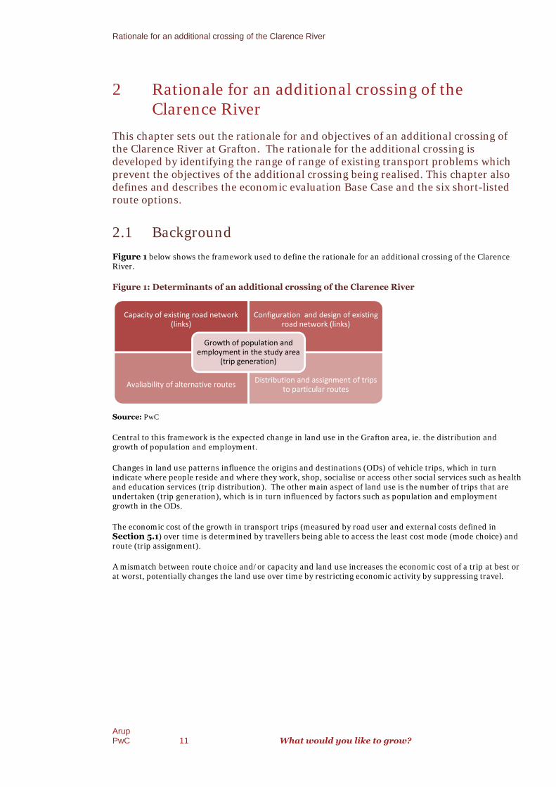
Figure 1 below shows the framework used to define the rationale for an additional crossing of the ClarenceRiver.
Figure 1: Determinants of an additional crossing of the Clarence River
Source: PwC
Central to this framework is the expected change in land use in the Grafton area, ie. the distribution andgrowth of population and employment.
Changes in land use patterns influence the origins and destinations (ODs) of vehicle trips, which in turnindicate where people reside and where they work, shop, socialise or access other social services such as healthand education services (trip distribution). The other main aspect of land use is the number of trips that areundertaken (trip generation), which is in turn influenced by factors such as population and employmentgrowth in the ODs.
The economic cost of the growth in transport trips (measured by road user and external costs defined inSection 5.1) over time is determined by travellers being able to access the least cost mode (mode choice) androute (trip assignment).
A mismatch between route choice and/or capacity and land use increases the economic cost of a trip at best orat worst, potentially changes the land use over time by restricting economic activity by suppressing travel.
Capacity of existing road network(links)
Configuration and design of existingroad network (links)
Avaliability of alternative routesDistribution and assignment of trips
to particular routes
Growth of population andemployment in the study area
(trip generation)

Rationale for an additional crossing of the Clarence River
ArupPwC 12
2.2 Land use in Grafton
2.2.1 Land use
The existing and future land use patresidential and employment/service zonesthe Clarence River. The other main aspect of land use iswhich include a river crossing. There is evidence that population growth in theexceeding the rates of growth at the State and regional levels, and that a large proportion of this growth will beconcentrated on one side of the Clarence River.
Figure 2 locates the town centres of Grafton and South Grafton
Figure 2: Clarence River Crossing
Source: Google Maps (2012)
Most of the highway-related businesses inWay). Bent Street also connects to Grafton via the existing bridge with South Grafton, Armidale Road and theGwydir Highway. Skinner Street in South Grafton functions as theBusiness District (CBD). South Grafton also features industrial and employment lands to the west of thePacific Highway between Clarenza and the existing residential areas. The industrial area is connected to SouthGrafton by the Pacific Highway or through local road linkages through to Armidale Road.
The existing residential areas in South Grafton are bounded to theto the west. There is also residential development along the Gwydir Highwresidential area in South Grafton isresidential development. The area is intersected by Centenary Drive, with connections to the Pacific Highwayprovided by Frances, Clarenza and Duncans Roads.
Rationale for an additional crossing of the Clarence River
What would you like to grow?
Land use in Grafton
The existing and future land use pattern in the Grafton area underpin the case for an additionalresidential and employment/service zones are geographically separated and concentrated on opposite sides ofthe Clarence River. The other main aspect of land use is the growth in demand for trips, particularly thosewhich include a river crossing. There is evidence that population growth in the Grafton area will be significant,exceeding the rates of growth at the State and regional levels, and that a large proportion of this growth will beconcentrated on one side of the Clarence River.
town centres of Grafton and South Grafton on opposite sides of the
: Clarence River Crossing – linking Grafton and South Grafton
related businesses in South Grafton are located along Bent Street (part of SummerlandWay). Bent Street also connects to Grafton via the existing bridge with South Grafton, Armidale Road and theGwydir Highway. Skinner Street in South Grafton functions as the main street in the South Grafton Central
South Grafton also features industrial and employment lands to the west of thePacific Highway between Clarenza and the existing residential areas. The industrial area is connected to South
Pacific Highway or through local road linkages through to Armidale Road.
The existing residential areas in South Grafton are bounded to the east by Mackay Street and Rushfor. There is also residential development along the Gwydir Highway. The primary
is the Clarenza Urban Release Area. It is directly east of the existingresidential development. The area is intersected by Centenary Drive, with connections to the Pacific Highway
Frances, Clarenza and Duncans Roads.
additional crossing asare geographically separated and concentrated on opposite sides of
growth in demand for trips, particularly thosearea will be significant,
exceeding the rates of growth at the State and regional levels, and that a large proportion of this growth will be
Clarence River.
South Grafton are located along Bent Street (part of SummerlandWay). Bent Street also connects to Grafton via the existing bridge with South Grafton, Armidale Road and the
he South Grafton CentralSouth Grafton also features industrial and employment lands to the west of the
Pacific Highway between Clarenza and the existing residential areas. The industrial area is connected to SouthPacific Highway or through local road linkages through to Armidale Road.
by Mackay Street and Rushforth Roadprimary developing
directly east of the existingresidential development. The area is intersected by Centenary Drive, with connections to the Pacific Highway

Rationale for an additional crossing of the Clarence River
ArupPwC 13 What would you like to grow?
Across the Clarence River, Grafton has a clearly defined urban core, with the primary commercial activitiescentred along Prince Street. Highway-related businesses are located along Fitzroy Street, which links the
existing bridge with Grafton’s CBD and also runs perpendicular to Prince Street3, bringing traffic (and hence,
passing trade) off the bridge and in to the main commercial street.
The existing and proposed residential areas are bounded by the Clarence River and North Street to the north.Running perpendicular to Prince Street, Victoria Street is Grafton’s civic street, where much of the town’sadministrative and institutional activities are concentrated. King Street also has an administrative function.
Grafton has a clearly defined urban core, with the primary commercial activities centred along Prince Street.Grafton covers the majority of trip attractants including but not limited to educational facilities (7 of the 10main educational facilities), Grafton Base Hospital, Grafton Shopping World, emergency services including thepolice station, and 66 per cent of the businesses surveyed (n=104) as part of the technical investigations forthis initiative4.
2.2.2 Population
Grafton is identified in the Mid North Coast Regional Strategy5
as a major regional centre and also has thegreatest capacity for commercial redevelopment. It is expected to take the majority of future commercialdevelopment in the Clarence sub region. Other major regional centres in the Mid North Coast Region are CoffsHarbour, Port Macquarie and Taree.
GTA Consultants (GTA)6 indicates that population in the Grafton area (Grafton, Junction Hill, South Grafton
and Clarenza) will grow at a rate of 1.67
per cent per annum between 2011 and 20498. These in turn are based
on population forecasts developed from information provided by Clarence Valley Council (CVC) and theDepartment of Planning and Infrastructure.
These forecasts are based on the dwelling targets established in the Mid North Coast Regional Strategy whichidentified the need for a minimum of 7,100 dwellings in the Clarence sub-region to 2031. While the Strategydocument identified a growth rate of 1.1 per cent across the Mid North Coast as a whole, it identifies Grafton asa major regional centre and one of the four main focal points for growth in the region.
Clarence Valley Council provided a breakdown of the dwelling locations which identified 6,297 new dwellingswithin Clarence Valley Council as well as their distribution within the Council area based on land capacity.Table 1 below shows the locations of new dwellings that are within the study area.
3While the recently developed Grafton Shopping World, located on Fitzroy Street, has shifted some of the commercial and retail focus away
from the main street environment (Prince Street) to an internalised shopping mall, its close proximity to Prince Street has helped to keepthe town centre intact.
4 Jetty Research 2011, Additional crossing of the Clarence River at Grafton, Online Business Survey Report, Prepared for the Roads and
Traffic Authority, June 2011, p.12.
5NSW Department of Planning 2009, Mid North Coast Regional Strategy, NSW Government.
6 GTA Consultants 2012, Main Road 83, Summerland Way, Additional Crossing of the Clarence River, Grafton, Route Options Development
Report – Technical Paper: Traffic Assessment, p.6.
7This rate of growth is significant when compared to forecasts by NSW Planning and Infrastructure which estimates growth at around 1 per
cent (2011 – 2036) for Sydney and the Mid-North Coast, NSW.
8The growth rate is based on advice from Clarence Valley Council (CVC). It assumes that land capacity of the area will be taken up over a 20
year period to 2031, and then extrapolated to 2041 for our 30 year time horizon. In reality, the uptake on the available land and thereforeincrease in population may take longer than assumed.

Rationale for an additional crossing of the Clarence River
ArupPwC 14 What would you like to grow?
Table 1: Forecast dwelling locations in Grafton
AreaDwellings2010 – 2021
Dwellings2021 – 2031
Clarenza 375 375Grafton 200 0Junction Hill 500 500South Grafton 300 330Total 1,375 1,205
The CVC recommended the following occupancy rates to convert dwellings to persons:
2.47 persons per household was adopted for the period 2010 – 2021; and
2.41 persons per household was adopted fort the period 2021 – 2031.
Adopting the above new dwellings and household rates results in an additional 3,396 persons by 2021 and afurther 2,904 persons between 2021 and 2031 as outlined.
Table 2 indicates that population growth in the Grafton area (Grafton, Junction Hill, South Grafton andClarenza) is expected to occur at a rate of approximately 1.6 per cent per annum linear from 2010 for the 31year period from 2010.
Table 2: Population growth in Grafton
Year
Location 2010 2021 2031 2041
Grafton 10,761 11,255 11,255 11,255Junction Hill 1,015 2,250 3,455 3,455South Grafton 6,065 6,806 7,601 7,601Clarenza 684 1,610 2,514 5,418Total 18,525 21,921 24,825 27,729Growth(LinearGrowth from
2010)9
3,396(1.6 per cent peryear)
2,904(1.6 per cent peryear)
2,904(1.6 per cent peryear)
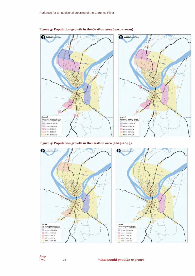
Growth to year 2021 is expected to occur in Grafton, Junction Hill, South Grafton and Clarenza. Growthbetween years 2021 and 2031 is expected to be concentrated in Junction Hill, South Grafton and Clarenza.Between years 2031 and 2041 the majority of growth will occur in Clarenza. The geographical profile of
population growth is shown in Figure 3 and Figure 4 below10
. The rate of growth of population indicatesthat the demand for cross river access from the residential areas in South Grafton will continue and increase.
9Growth beyond 2031 is assumed to be at the same linear growth rate.
10 GTA Consultants 2011a, Additional crossing of the Clarence River at Grafton, Preliminary Route Options Report – Part Two, Volume 2
Technical paper - Strategic Traffic Assessment, November 2011, p. 30.
Rationale for an additional crossing of the Clarence River
ArupPwC 15
Figure 3: Population growth in
Figure 4: Population growth in the Grafton
Rationale for an additional crossing of the Clarence River
What would you like to grow?
Population growth in the Grafton area (2011 – 2029)
Population growth in the Grafton area (2029-2049)
What would you like to grow?

Rationale for an additional crossing of the Clarence River
ArupPwC 16 What would you like to grow?
2.3 Defining the existing transport challenges
While Grafton and South Grafton have respective residential and employment centres, forecast growth inpopulation is expected to add to the existing focus on residential land uses in South Grafton. This will increasedemand for trips crossing the River to access employment and services concentrated in Grafton. Populationgrowth in the Grafton area is expected to increase the demand for bridge crossings by 108 per cent over thenext 30 years11.
The increase in the demand for river crossings is not in itself a problem. Negative social, environmental andeconomic outcomes occur when the capacity and design of the existing transport network cannot accommodatethe growth in the number of trips. The reasons for a network’s inability to accommodate these changes(effectively and efficiently) comprise the problem. The key transport problems in the Grafton area relate to:
the capacity of key road links;
the design of key road links;
the extent to which travel between key ODs rely on specific routes; and
the lack of available alternative routes linking the key ODs.
2.3.1 Inefficient configuration and capacity of existinginfrastructure
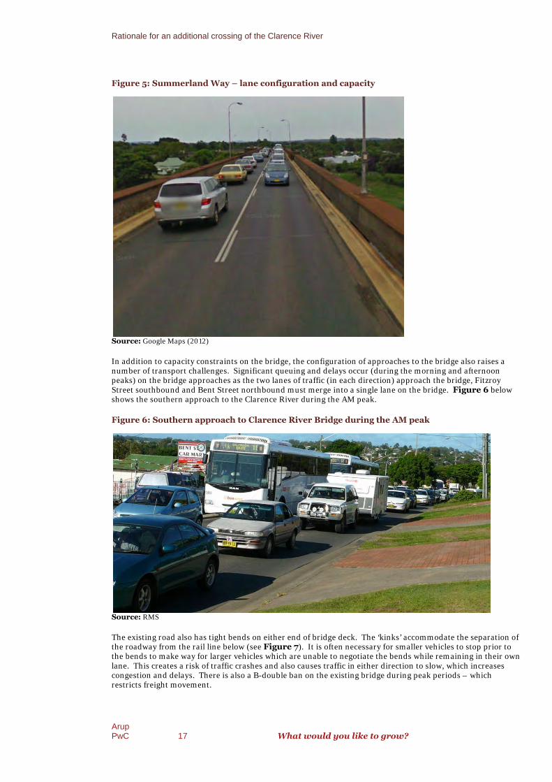
The existing road linking Grafton and South Grafton comprises a four hundred and thirty-eight metre (m) longdouble deck steel bridge (see Appendix A). The lower deck comprises a railway track and twopedestrian/cyclist lanes, while the upper deck comprises two-way road lanes.
Lane widths (see Figure 5) constrain capacity to carry the expected growth in the number of trips. The
theoretical capacity12
of the bridge could be considered in the range of 900 to 1,400 vehicles per hour in onedirection. Traffic counts undertaken in August 2010 indicate that the bridge was carrying 1,360 vehicles perhour in the northbound direction during the AM peak and 1,330 vehicles per hour in the southbound directionin the PM peak. Based on the traffic flows recorded on the bridge and the information set out in the AustroadsGuide, it is apparent that the peak hour traffic flows across the bridge are at, or very close to, capacity on thebridge.
11GTA Consultants (2012, p. 6).
12Austroads 2009, Guide to Traffic Management Part 3: Traffic Studies and Analysis, Austroads.
Rationale for an additional crossing of the Clarence River
ArupPwC 17 What would you like to grow?
Figure 5: Summerland Way – lane configuration and capacity
Source: Google Maps (2012)
In addition to capacity constraints on the bridge, the configuration of approaches to the bridge also raises anumber of transport challenges. Significant queuing and delays occur (during the morning and afternoonpeaks) on the bridge approaches as the two lanes of traffic (in each direction) approach the bridge, FitzroyStreet southbound and Bent Street northbound must merge into a single lane on the bridge. Figure 6 belowshows the southern approach to the Clarence River during the AM peak.
Figure 6: Southern approach to Clarence River Bridge during the AM peak
Source: RMS
The existing road also has tight bends on either end of bridge deck. The ‘kinks’ accommodate the separation ofthe roadway from the rail line below (see Figure 7). It is often necessary for smaller vehicles to stop prior tothe bends to make way for larger vehicles which are unable to negotiate the bends while remaining in their ownlane. This creates a risk of traffic crashes and also causes traffic in either direction to slow, which increasescongestion and delays. There is also a B-double ban on the existing bridge during peak periods – whichrestricts freight movement.

Rationale for an additional crossing of the Clarence River
ArupPwC 18
Figure 7: Grafton Bridge ‘kinks’
Source: Google Maps (2012)
2.3.2 Reliance on the
The reliance on the existing route across the Clarence River is attributable to two main
the trip ODs implied by the existi
the absence of practical alternative routes across the Clarence River.
The absence of a practical alternative route is the key challenge to accommodating the expected growth in tripdemand. The trip length between Grafton and South Grafton (using the existing bridge) is approximately 3 km(see Figure 2). The figure below shows an alternative route via Rogan Bridge Road and the Gwydir Highway.The trip distance in comparison to the existing route is significantly longer at around 60 km.
sing of the Clarence River
What would you like to grow?
: Grafton Bridge ‘kinks’
the existing bridge
The reliance on the existing route across the Clarence River is attributable to two main factors:
mplied by the existing land use pattern (discussed above); and
the absence of practical alternative routes across the Clarence River.
he absence of a practical alternative route is the key challenge to accommodating the expected growth in tripen Grafton and South Grafton (using the existing bridge) is approximately 3 km
The figure below shows an alternative route via Rogan Bridge Road and the Gwydir Highway.ison to the existing route is significantly longer at around 60 km.
factors:
he absence of a practical alternative route is the key challenge to accommodating the expected growth in tripen Grafton and South Grafton (using the existing bridge) is approximately 3 km
The figure below shows an alternative route via Rogan Bridge Road and the Gwydir Highway.ison to the existing route is significantly longer at around 60 km.

Rationale for an additional crossing of the Clarence River
ArupPwC 19
Figure 8: Alternative River crossing route
Source: Google Maps (2012)
The reliance on the existing cross river route is clThe survey indicates that 97 per cent of trips which crossed the Grafton Bridge started andGrafton or South Grafton. In particular GTA found that:
approximately 63 per cent of northGrafton
approximately 90 per cent of southbound vehicles crossing the Clarence River have an origin inGrafton and 65 per cent travel to a destination in South Grafton
approximately 62 perorigin in South Grafton and 80 per cent travel to a destination in Grafton
approximately 72 per cent of heavy vehicles travelling southbound across the Clarence River have anorigin in Grafton and 56 per cent travel to a destination in South Grafton.
13 The survey was undertaken between 5 am and 7pm on 19
14GTA Consultants (2012, p. 4).
Rationale for an additional crossing of the Clarence River
What would you like to grow?
: Alternative River crossing route – Rogan Bridge Road and Gwydir Highway
Google Maps (2012)
The reliance on the existing cross river route is clearly demonstrated in an ODThe survey indicates that 97 per cent of trips which crossed the Grafton Bridge started andGrafton or South Grafton. In particular GTA found that:
approximately 63 per cent of northbound vehicles crossing the Clarence River have an origin in South
approximately 90 per cent of southbound vehicles crossing the Clarence River have an origin inGrafton and 65 per cent travel to a destination in South Graftonapproximately 62 per cent of heavy vehicles travelling northbound across the Clarence River have anorigin in South Grafton and 80 per cent travel to a destination in Graftonapproximately 72 per cent of heavy vehicles travelling southbound across the Clarence River have anorigin in Grafton and 56 per cent travel to a destination in South Grafton.
The survey was undertaken between 5 am and 7pm on 19th August 2010.
GTA Consultants (2012, p. 4).
What would you like to grow?
Rogan Bridge Road and Gwydir Highway
survey conducted13 by GTA14.The survey indicates that 97 per cent of trips which crossed the Grafton Bridge started and/or finished in
bound vehicles crossing the Clarence River have an origin in South
approximately 90 per cent of southbound vehicles crossing the Clarence River have an origin in
cent of heavy vehicles travelling northbound across the Clarence River have anorigin in South Grafton and 80 per cent travel to a destination in Graftonapproximately 72 per cent of heavy vehicles travelling southbound across the Clarence River have anorigin in Grafton and 56 per cent travel to a destination in South Grafton.

Rationale for an additional crossing of the Clarence River
ArupPwC 20 What would you like to grow?
Moreover, the traffic demand modelling undertaken by GTA15 indicates that trip ODs which involve a bridgecrossing account for large proportion of network trips. Figure 9 below indicates that during the AM and PMpeak periods, over 30 per cent of network trips cross the Clarence River use the existing route. This proportionincreases to nearly 40 percent by 2049.
Figure 9: Number of bridge crossings as a proportion of total trips
Year AM Peak (7am to 9am) PM Peak (3pm – 5pm)
Tripscrossingbridge
Total trips% crossingbridge
Tripscrossingbridge
Total trips% crossingbridge
2011 3,783 12,456 30.37 4,603 14,641 31.44
2019 4,285 14,040 30.52 5,549 15,963 34.76
2029 6,103 18,130 33.81 7,507 20,554 36.52
2039 7,152 21,232 33.69 8,627 23,833 36.20
2049 8,099 23,047 35.14 9,544 25,577 37.31
Source: GTA (2012)
2.3.3 Network redundancy
The existing cross-river route provides network redundancy during incident responses on the Pacific Highway– particularly during flood events and traffic incidents. This role exacerbates the problems discussed above.For example, in January 2012, flooding led to the closure of the Pacific Highway near Grafton and at Corindi.Southbound light and heavy vehicles were diverted at Ballina onto the Bruxner Highway to Casino, then ontoSummerland Way to Grafton. The extent of diversion shown below in Figure 10 demonstrates theimportance of the river crossing to the regional road network.
It is noted that the reliance on the bridge as a detour will be significantly reduced following the upgrade of thePacific Highway to dual carriageway.
15 ibid.

Rationale for an additional crossing of the Clarence River
ArupPwC 21 What would you like to grow?
Figure 10: Diversions to Summerland Way during flooding of Pacific Highway
Source: Google Maps (2012)
2.4 Outcomes of the existing transport challenges
The transport problems identified above have led to a number of negative outcomes:
there are significant traffic delays and constraints on the existing Grafton Bridge during peak periods;
there are delays to emergency vehicles responding to incidents on the Pacific Highway due to the
delays caused on the existing bridge16
;
there is conflict with heavy vehicles on the bends on the existing bridge;
there is a B-double ban on the existing bridge during peak periods – which restricts freightmovement;
the existing bridge is causing an impact on access to services and facilities due to delays17
;
16However, this risk is mitigated to some extent by contingency plans by emergency services including the placement of personnel and
vehicles on either side of the bridge during the peak periods.
17Jetty Research (2011).

Rationale for an additional crossing of the Clarence River
ArupPwC 22 What would you like to grow?
there are safety issues with the pedestrian/cycle access on the existing bridge – no dedicated
pedestrian or bicycle paths are provided at the vehicular level (bridge upper deck)18
; and
the existing bridge and approach roads do not facilitate the economic viability of the South Graftonbusiness area (Skinner St) – this area is bypassed by the current approach roads.
These challenges impact negatively on the following traffic outcomes:
network vehicle hours travelled (VHT) and vehicle kilometres travelled (VKT) over the entire roadnetwork;
estimated average trip travel times across the network and between key ODs such as: Grafton andSouth Grafton; the Pacific Highway and the Summerland Way; and
estimated average total delay across the network.
Deterioration in network performance increases the economic cost of travel. Significant increases in trip costscan change travel behaviour, particularly for commercial trips. For example, a survey of businesses and bus
companies in the region found that19:
most companies established routes to avoid areas of peak hour traffic congestion;
some companies have arranged business times so that deliveries are made outside of the peak periods,although at times this was noted to be unavoidable;
the bridge curfew during morning and afternoon peak periods has a significant effect on businessoperations (e.g. scheduling);
late running of services due to bridge congestion led to additional cost in the operation of catch upand head off services; and
perceptions of incidents on the bridge were a concern due to a lack of access to and from each side ofthe bridge in emergency situations for ambulances and the like.
More broadly, traffic delays in peak periods are changing people's travel behaviour and daily activity patterns,and as a result may be constraining development. It would appear from the traffic count data that bridge usershave timed their trip to avoid the peak period traffic congestion. Grafton and South Grafton are to some extent
operating as separate towns20
.
18Roads and Maritime Services (RMS) 2012a, Additional crossing of the Clarence River at Grafton, Preliminary Route Options Report, Final
January 2012, p.40.
19GTA (2011a, p. 3).
20ibid (p. 5).

Rationale for an additional crossing of the Clarence River
ArupPwC 23 What would you like to grow?
2.5 Objectives and outcomes sought from a solution
The key objectives for the additional crossing of the Clarence River at Grafton are to:
enhance road safety for all road users over the length of the project;
improve traffic efficiency between and within Grafton and South Grafton;
support regional and local economic development;
involve all stakeholders and consider their interests;
provide value for money; and
minimise impact on the environment.
The following supporting objectives assist in achieving the project objectives.
Enhance road safety for all road users over the length of the project
reduce the potential for road crashes and injuries on the bridge and approaches including anyintersections and connecting roads
provide safe facilities for pedestrians and cyclists
Improve traffic efficiency between and within Grafton and South Grafton
provide efficient access for a additional crossing of the Clarence River and for the State road network
provide a traffic management network which reduces delays between Grafton and South Grafton inpeak periods to an acceptable level of service for 30 years after opening
provide adequate vertical clearance for heavy vehicles
consider demand management strategies to minimise delays to local and through traffic.
Support regional and local economic development
provide transport solutions that complement existing and future land uses and support developmentopportunities
provide improved opportunities for economic and tourist development for Grafton
provide for commercial transport including B-Doubles where required
provide flood immunity for the bridge for a one in 100-year flood event, and for the approach roadsfor a one in 20-year flood event, where economically justified
provide navigational clearance from the additional crossing for river users.
Involve all stakeholders and consider their interests
develop solutions that consider community expectations for the project
satisfy the technical and procedural requirements of RMS with respect to the planning and design ofthe project

Rationale for an additional crossing of the Clarence River
ArupPwC 24 What would you like to grow?
integrate input from the community into the development of the project through the implementationof a comprehensive program of community consultation and participation.
Provide value for money
achieve a justifiable benefit-cost ratio at an affordable cost
develop a strategy to integrate future upgrades into the project.
Minimise impact on the environment
minimise the impact on the social and economic environment, including property impacts
minimise the impact on residential amenity, including noise, vibration, air quality etc
minimise the impact on heritage
minimise impact on the natural environment
provide a project that fits sensitively into the built, natural and community context
minimise flooding impact caused by the project.
2.6 Definition of the Base Case
The Base Case for this economic evaluation comprises the 2011 road network. It also includes four upgradeprojects that would be required by 2019 with and without the additional crossing route options. These upgradeprojects include:
upgrading Pound Street to two lanes in each direction between Villiers Street and Prince Street;
upgrading of Gwydir highway to two traffic lanes in each direction between Pacific Highway and BentStreet;
upgrading of the Villiers Street and Dobie Street roundabout to improve turning movements for heavyvehicles; and
upgrading the Gwydir Highway and Skinner Street roundabout from a single roundabout to a twolane roundabout.
The Base Case, as with the route options, also assumes that the Glenugie to Tyndale Upgrade of the PacificHighway (which bypasses South Grafton) is opened to traffic by 2019.
The direct infrastructure costs included in this economic evaluation are incremental, ie. they are net of directinfrastructure costs that would also occur with the Base Case. Therefore, the Base Case is not explicitly costed.However, as discussed in Section 6.1, the costs of these projects are deducted from route option costs toensure the route option costs are incremental.

Rationale for an additional crossing of the Clarence River
ArupPwC 25 What would you like to grow?
2.7 Description of the proposed route options
The process used to identify the six short-listed route options is discussed in Chapter 1.1 of the Route OptionsDevelopment Report. These six route options are described below in Table 3.
Table 3: Additional crossing route options by corridor
RouteOption
Description
E Option E includes a new bridge upstream of the existing bridge where it would connect the GwydirHighway at Cowan Street in South Grafton to Villiers Street in Grafton. The vertical clearance ofVilliers Street would be upgraded to 5.3m to accommodate heavy vehicles under the railwayviaduct.
Both the new and existing bridge would have one lane in each direction.
A Option A consists of a new bridge constructed slightly upstream and parallel to the existing bridge.This option would connect Bent Street in South Grafton to Fitzroy Street in Grafton. The verticalclearance of Villiers Street would be upgraded to 5.3 m to accommodate heavy vehicles under therailway viaduct.
The new bridge would have two northbound lanes and one southbound lane and the existing bridgewill be converted to one southbound lane.
C Option C involves building a new bridge slightly downstream and parallel to the existing bridge.This option connects the Pacific Highway at Iolanthe Street in South Grafton to Clarence andPound Street in Grafton. Villiers Street would have its vertical clearance upgraded to 5.3m toaccommodate heavy vehicles under the railway viaduct.
Under Option C, both bridges would have one lane in each direction.
11 Option 11 involves the construction of a new bridge downstream of the existing bridge where itwould connect the Pacific Highway at McClaers Lane in South Grafton to Fry Street in Grafton.
Option 11 would include two viaduct structures between the Pacific Highway and the ClarenceRiver. It would also include an upgrade of Fry Street to enable it to meet future traffic volumes andof Villiers Street to accommodate a 5.3m vertical clearance for heavy vehicles beneath the railwayviaduct.
Both bridges would have one lane in each direction.
14 Option 14 involves the construction of a new bridge downstream of the existing bridge where itconnects Pacific Highway at Centenary Drive in South Grafton and North Street via Kirchner Streetat Grafton.
Both the new and existing bridge would be one lane in each direction.
Option 14 involves a number of constructions and upgrades:
Kirchner, North and Turk Street would require an upgrade to accommodate future trafficvolumes;
a viaduct structure would be required from the Pacific Highway to the Clarence River; and
Villiers Street would need to be upgraded to increase the vertical clearance for heavy

Rationale for an additional crossing of the Clarence River
ArupPwC 26 What would you like to grow?
RouteOption
Description
vehicles to 5.3m.
Prince, Kirchner and Dobie Street would need to be upgraded for heavy vehicle access into
central Grafton.21
15 Option 15 involves the construction of a new bridge downstream of the existing bridge where itconnects Pacific Highway at Centenary Drive in South Grafton to Summerland Way via KirchnerStreet in Grafton.
All construction aspects are the same as Option 14; the only difference is the alignment of thebridge after it connects in Grafton. As a result, Option 15 has the same implications as Option 14 inconstructing an additional crossing of the Clarence River.
Source: RMS (2012)
21ARUP (2012) Additional Crossing of the Clarence River at Grafton – Preliminary Route Options Report Final, prepared for Roads and
Maritime Services, p121

Rationale for an additional crossing of the Clarence River
ArupPwC 27 What would you like to grow?
The short-listed route options are illustrated in Figure 11.
Figure 11: Map of short listed route options
Source: Arup

Economic evaluation methodology
ArupPwC 28 What would you like to grow?
3 Economic evaluation methodology
This chapter outlines the methodology for the economic evaluation. It is based onthe Road User Cost Benefit Analysis (RUCBA) approach. This approach usesdiscounted cash flow analysis (DCFA). The key assumptions of DCFA such asdiscount rate and evaluation period are defined. This chapter also highlights keyaspects of the economic evaluation methodology including the specific treatmentand role of traffic demand produced from a microsimulation traffic model andselection of appropriate traffic expansion factors to estimate benefits of relievingnetwork congestion during peak periods.
3.1 Economic evaluation approach
The economic evaluation of the six route options in this Report is undertaken using CBA. CBA measures theeconomic viability of a route option by comparing the additional benefits of the route option with the
additional costs22
with a route option, over a defined evaluation period.
Microsimulation traffic modelling was used to estimate the traffic demand for this economic evaluation. Thisapproach was selected over a strategic (unconstrained) link based traffic model given the significant transportproblems in the Grafton area (see Section 2.3). As a vehicular based approach, microsimulation is ideal forsimulating traveller behaviour in congested road networks. However, it poses a number of challenges toproducing outputs for economic evaluation including the difficulty in producing sufficient capacity for longterm traffic forecasts and the potential for the modelling to suppress travel altogether beyond certain levels ofroad congestion. These challenges are identified and addressed in Section 4.2.1. Microsimulation trafficmodelling is discussed further in the Route Options Development Report: Technical Paper – TrafficAssessment.
The microsimulation modelling of the Grafton area was unable to produce traffic demand forecasts (for allforecast years) with the Base Case. While the discussion in Chapter 4 outlines an approach for dealing withthis issue, it is applied with a number of qualifications and caveats. Therefore, the results should only be usedto demonstrate the relative economic merit of the route options (ie. a comparative assessment), rather thanproviding an accurate measure of the absolute net economic benefit of a particular route option.
A route option is considered economically viable if the additional benefits exceed the additional costs.
Road based transport options are commonly appraised using Road User Cost Benefit Analysis (RUCBA).RUCBA is an applied CBA framework which defines and measures the key benefits of road transport options asreductions in:
vehicle travel time costs (VTTC);
vehicle operating costs (VOC);
crash costs (CC); and
costs of environmental and social effects from vehicle use (externalities).
22The additional or incremental benefits and costs are measured with respect to the Base Case.

Economic evaluation methodology
ArupPwC 29 What would you like to grow?
The first three economic costs are collectively referred to as ‘road user costs’, while environmental and socialeffects from transport use are referred to as ‘external costs’.
Changes in road user and external costs are compared to the fixed and recurrent infrastructure costs to assesseconomic viability of the route options.
The RUCBA is applied using discounted cash-flow analysis (DCFA). The DCFA is based on a spreadsheetmodel which ‘streams’ the annual benefits and costs with the Base Case and the route option. These annualvalues are presented over a defined period into the future (commonly 30 years from the first full year ofoperation of the route option).
The DCFA converts all future values to a common time dimension. The common time dimension in DCF isreferred to as Present Value (PV). Present values are calculated by discounting future values (which reflects thetime value of money, ie. a dollar today is worth more than a dollar in the future) using a recommendeddiscount rate.
The general assumptions used in this DCFA:
cashflows are expressed for financial years ending June (YEJ);
cashflows are included in the period within which the associated expenditures or benefits occur;
the Base Year of the economic evaluation is 2010/1123
;
all values are expressed in real dollars24
;
prices are expressed in 2011/12 dollars (unless otherwise stated);
all road user cost parameters are sourced from the latest version of the RMS’s Economic Analysis
Manual, ie. 200925
.
the evaluation period starts in 2019/2026
and ends in 2048/49. This is in line with the RMSGuidelines which requires that projects are evaluated over a 30 year period from the first year of fulloperation of the road initiative;
future net benefits are discounted to the respective base years using a real discount rate of 7 per
cent27
;
incremental road maintenance cost is assumed to be zero for each scenario (see Section 6.2); and
the demand modelling assumes that the transport effects of the ultimate route option design will berealised in the first year of operation. In reality, some infrastructure components of the route optionsmay be staged over time.
23To maintain consistency, the Base Year is assumed to be 2010/11 to maintain consistency with the Base Year of the traffic demand
modelling.
24Real values exclude inflation.
25The latest road user and external cost parameters are included in Appendix B of RMS’s Economic Analysis Manual 2009. Inquiries made
during this study indicate that Austroads are yet to release updated parameter values for Road User Effects, and that provisional indicatorssuggest that the current valuation of benefits are approximately 6.4 per cent higher than those shown in the 2009 version of the RMS’sEconomic Analysis Manual.
26For the purposes of assessment, it is assumed that the additional crossing would be opened to traffic in 2019. Since the economic
evaluation is based on financial years, the first full year of operation is 2019/2020.
27In line with guidance from Infrastructure Australia, NSW Treasury and RMS.

Economic evaluation methodology
ArupPwC 30 What would you like to grow?
This RUCBA reports on the following measures of economic performance:
Net Present Value (NPV) – the difference between the present value (PV) of total incremental benefits(avoided road user and external costs) and the present value of the total incremental infrastructurecosts. The NPV is used as the primary measure of merit where budgets are un-constrained; and
Benefit Cost Ratio (BCR) – ratio of the PV of total incremental benefits over the PV of totalincremental costs. The BCR is used as the primary measure of merit where budgets are constrained.
Route options with a positive NPV indicate that the incremental benefits exceed the incremental infrastructurecosts over the evaluation period. A BCR greater than 1.0 indicates that a project is also economically viable. Ifthere is no constraint on the availability of funds, NSW Treasury guidelines suggest the use of NPV as thisenables economic benefits to be maximised. The BCR is the most commonly used evaluation criteria within theRMS.
3.2 RUCBA methodology
The RUCBA approach is outlined in RMS’s Economic Analysis Manual28
. However, specific methodologiesare required at certain stages. These methodologies are identified below and reference is provided to therelevant section in the report where these specific treatments are discussed.
Having defined and documented the: transport problems (see Section 2.3); objectives and outcomes of asolution (see Section 2.5) and the proposed solutions and the Base Case (see Section 2.6), the followingcomprise the key steps in the RUCBA:
‘streaming’29
of costs with the Base Case and route options. These are based on cashflow profiles
provided by Arup30
. The key issue with this task is ensuring that the costs are appropriatelymeasured and defined for economic (rather than financial) evaluation. This includes ensuring thatcosts are in real and resource terms, excluding inflation and transfers such as taxes and profit. Thedetailed costing methodology is outlined in Chapter 6.
collection and ‘streaming’ of traffic demand forecasts. This is the first step in benefit estimation.Conventional traffic outputs for economic evaluations include network VKT, VHT, stops and trips,with the Base Case and the route option. The key methodological issues outlined in Chapter 4includes:
o clear identification of the land use and population assumptions adopted and whether thesechange between the Base Case and the route options;
o identification of the appropriate peak period to daily forecast to ensure that the economicbenefits are not overestimated; and
o developing an approach to address suppressed demand with the Base Case due to capacityconstraints with microsimulation traffic modelling.
estimation of ‘conventional’ road user and external costs. The methodology for this task is outlined inChapter 5 and involves sourcing and applying the relevant economic unit costs to the annual
28RMS 1999, Economic Analysis Manual, Version 2, RMS, NSW.
29Streaming refers to assigning the cost or benefit to the year in which it is expected to occur. Capital costs are streamed in line with the
construction profile of the route options (see Section 6.1.3). Benefits in this economic evaluation are defined as reductions in road userand external costs (compared with the Base Case). The road use and external costs are in turn a function of changes in traffic demand andhence, benefits are streamed in line with the traffic demand forecast profiles. The role of traffic demand forecasts in estimating road userand external costs is discussed in Section 4.2.
30Email dated 13th February 2012.

Economic evaluation methodology
ArupPwC 31 What would you like to grow?
demand estimates developed above. Conventional benefits estimated include reductions in: traveltime cost, vehicle operating cost, stop costs, crash costs and environmental and social externalitiessuch as Greenhouse Gas Emissions (GHG) and water pollution;
Chapter 7 discusses the spreadsheeting analysis used to combine the annual benefits and costs withthe route options. CBA is based on a DCF which forecasts the annual benefits and costs over anevaluation period extending 30 years from the first full year of operation of the route option. Thesefuture costs and benefits are then ‘discounted’ using a real discount rate of 7 per cent. These benefitsand costs are combined (using specific equations) to produce measures of economic merit includingthe BCR and NPV. This task also includes sensitivity analyses which assess the robustness of theeconomic viability of the route option under alternative assumptions relating to different levels ofcapital cost, demand, land use assumptions, discount rate etc…

Demand (traffic) analysis
ArupPwC 32 What would you like to grow?
4 Demand (traffic) analysis
This Chapter details the role of traffic demand forecasts in the economicevaluation. It also presents estimated traffic demand for each of the additionalcrossing route options. Finally, it discusses the approach used to address thechallenges posed by using microsimulation traffic demand forecasts for economicevaluation.
4.1 Background
4.1.1 Traffic forecasting approach
The traffic forecasts used in this economic evaluation are produced by GTA using Q-Paramics, amicrosimulation traffic model. The traffic modelling approach and outputs are detailed in GTA’s technical
paper31
.
4.1.2 Study area
The study area modelled includes the existing Grafton Bridge connecting Grafton and South Grafton, as well asthe areas of Junction Hill, Carrs Creek, Great Marlow, Clarenza, Waterview Heights and South Grafton. Themodel considers traffic movements within these areas and includes traffic movements to and from the PacificHighway north and south, the Summerland Way, the Gwydir Highway and Armidale Road.
The study area is shown in Appendix B.
4.1.3 Model period and years
The flow of traffic varies throughout the day. Theoretically, traffic demand could be forecast on an hourly basisfor a 24-hour period. However, traffic demand is usually estimated for specific blocks or periods during theday which share common traffic flow characteristics.
GTA forecast traffic demand for a two hour period in both the AM peak (7am to 9am) and PM peak (3pm-5pm). The decision on the model period is based on the need to assess effects in different time periodscompared with using average annual daily estimates. In the case of the Grafton Bridge, peak travel places thegreatest demand on bridge capacity.
The model has a base year of 2011 and forecast years 2019, 2029, 2039 and 2049.
4.1.4 Expansion factors
The microsimulation model is a peak period model.
GTA developed a series of factors that are used to translate the peak period volumes to daily volumes.Congestion on the existing bridge and approaches is largely a peak phenomenon. Adopting an expansionfactor which would apply peak congestion relief benefits to trips which are taken outside the peak, and hencewould not have experienced the same level of congestion, would likely overestimate the net economic benefitsof the route options.
31GTA (2012, p.7).

Demand (traffic) analysis
ArupPwC 33 What would you like to grow?
Therefore, GTA undertook an exercise which involved re-running the traffic demand model for each of the sixroute options in unconstrained conditions. The exercise identified the hourly VKT and VHT for theunconstrained conditions for each of the route options. Finally, using existing daily traffic counts, theunconstrained VKT and VHT were apportioned over the entire day to determine appropriate peak to daily
values. These daily values are then annualised using a factor of 33532
.
4.1.5 Traffic growth – future years
A number of key assumptions were used in undertaking the microsimulation modelling assessment, inparticular those for the future year model. A summary of the key assumptions used by GTA to determine the
future year growth is provided by GTA33
:
the forecasts do not reflect the potential traffic impacts (particularly on heavy vehicles) of theproposed inland port located in the vicinity of the NSW and Queensland border;
the forecasts (conservatively) assume that the future industrial estate and freight hub planned forCasino will have no impact on heavy vehicle movements on the Summerland Way;
all future year modelling has assumed that the future upgrade of the Pacific Highway which wouldbypass of South Grafton would be open by 2019;
it is assumed that infill development would offset the population reductions due to declininghousehold size predicted by the Australian Bureau of Statistics. Therefore, the zonal populationforecasts for the traditional areas of Grafton and South Grafton are assumed to remain constant;
the key residential growth areas include Junction Hill, South Grafton,Waterview Heights, andClarenza. The development sequence assumed is Junction Hill and South Grafton, followed byWaterview Heights and finally Clarenza; and
growth in cross-river demand was constrained in the model between 2011 and 2019 due to the limitedcapacity of the existing bridge and as such traffic was redistributed within Grafton and South Graftonin order to realistically capture anticipated growth.
The network traffic growth assumptions are shown below in Table 4.
Table 4: Network traffic growth assumptions
Year AM Peak (7am to 9am) PM Peak (3pm to 5pm)
Total Trips(Vehicles)
TrafficGrowth Rate(% per year)
Total Trips(Vehicles)
TrafficGrowth Rate(% per year)
2011 12,456 14,641
2019 14,040 1.5 15,963 1.1
2029 18,130 2.6 20,554 2.6
2039 21,232 1.6 23,833 1.5
2049 23,047 0.8 25,577 0.7
Source: GTA (2012, p. 18)
32GTA (2012).
33GTA (2011a, p.28).

Demand (traffic) analysis
ArupPwC 34 What would you like to grow?
4.2 The role of traffic demand in RUCBA
Traffic demand measures the use of the road network, with and without the route options. It therefore alsoindicates the resources used in the course of undertaking a trip on the road network. The primary objective ofmost road infrastructure initiatives is to reduce the resource cost of trips on the network.
The total economic cost of a trip within RUCBA is determined by the type of road treatment being analysed anddefined according to transport economic theory. Table 5 below identifies the conventional road user costswhich comprise the total economic cost of a trip. Importantly, it also identifies the unit cost driver, whichrelates to the estimated measure of traffic demand.

Demand (traffic) analysis
ArupPwC 35 What would you like to grow?
Table 5: Determinants of road user costs
Road user cost (RUC) Unit Description Determinant
Savings in travel time costs(VTT)
$/vehicle hour travelled private occupant travel time costs; business occupant travel time costs;
commercial driver wage cost; and
freight contents delay costs – reflects the impacts ofgoods delays on the productive process of theeconomy.
vehicle type (e.g. car, light commercial, rigid truck,etc);
vehicle composition (% of traffic accounted for byrespective vehicle types);
distribution of traffic flow by time of day; and
vehicle occupancy.
Vehicle operating costs (VOC) $/vehicle kilometre travelled fuel and lubricant costs;
tyre costs; vehicle repair and maintenance costs;
depreciation, consumption of capital investment; and vehicle operator overhead costs.
vehicle type (e.g. car, light commercial, rigid truck,etc.);
vehicle composition (% of traffic accounted for byrespective vehicle types);
travel speed; pavement condition; and
grade and curvature.
Vehicle stops $/stop fuel and lubricant costs; tyre costs;
vehicle repair and maintenance costs; and
depreciation, consumption of capital investment.
number of stops
Crash costs $/incident fatal crash costs;
injury crash costs; and
property damage crash costs
crash rates;
type of road;
vehicle type; and vehicle occupancy.
Environmental external costs $/vehicle kilometre travelled noise;
air pollution;
water pollution; greenhouse;
nature and landscape; and urban separation costs.
vehicle type; and
urban/rural setting.
Source: RMS (RTA) (1999)

Demand (traffic) analysis
ArupPwC 36 What would you like to grow?
4.2.1 Treatment of suppressed demand with the Base Case
For most projects there are sufficient alternative traffic routes to allow the Base Case model to be established infuture years, although travel speeds may be low and travel times high. However, for this project, there are nosuitable alternative routes to cross the Clarence River in Grafton and cross-river traffic does not have anychoice but to use the existing bridge (see Section 2.3).
Economic evaluations undertaken as part of the Preliminary Route Options Report (PROR)34
used trafficdemand forecasts produced by strategic traffic models. These models are link based and allow traffic to passthrough the network at slower and slower speeds with demand well beyond the practical capacity of thenetwork. The result is that in later years the travel speeds with the Base Case model reduced to unrealisticallylow average network speeds of less than 5 km/h.
Increasingly, microsimulation modelling is being used in congested traffic conditions, such as the Graftonnetwork. This is because it becomes difficult to forecast sensible performance metrics using strategic link
based models35
. Unlike strategic traffic models, microsimulation is vehicular based and as such, physicallyprevents vehicles from passing through a congested network. However, adoption of microsimulationmodelling for this study means that when the peak cross-river traffic demand exceeds the physical capacity ofthe link between Grafton and South Grafton then vehicles are unable to pass through the congested networkand the result is gridlock in the model. The microsimulation model showed that the existing road networkwould be over-congested even by 2029 and as a result the Base Case option could not be modelled for 2029,2039 or 2049. Only a 2019 Base Case microsimulation model was established.
This is a stylised outcome of the modelling. In reality, travellers would undertake any number of adaptationswith the Base Case, including but not limited to:
re-timing their trip;
changing the number of trips undertaken;
changing their route and/or origin and destination.
There could also be more significant land use changes including declines in population and employmentgrowth rates and changes in land use patterns (e.g. location, timing and area of development of residential,commercial and employment lands). These non-marginal changes would in turn impact on the trip generationphase of the traffic demand model and hence, impact total demand.
In this situation, an alternative approach to estimating the economic benefits is adopted. In discussions withRMS it was agreed that benefits would be estimated by generating an indicative Base Case for future years.Establishment of this indicative Base Case acknowledges the reality that the existing road network wouldcontinue to function beyond 2019 even without an additional bridge. Travellers would adapt to increasingcongestion in the middle of the peak periods by for example re-scheduling trips to less congested periods andwould also accept higher levels of future congestion because of the absence of an alternative route.
Development of the indicative Base Case is intended to replicate the increase in delays and congestion thatwould occur over time without an additional bridge. It is established by taking the 2019 Base Case model andfactoring up the annual VKT and VHT parameters at similar rates to the increases observed in Route Options14 and 15. The reason for adopting the rates of increase for these route options is that due to their distancefrom the existing bridge and the town centres of Grafton and South Grafton, the majority of the traffic is shownto continue using the existing bridge. Therefore, they are the most constrained in terms of capacity betweenSouth Grafton and Grafton and therefore are likely to more closely represent what would happen in theindicative Base Case without a new bridge. In fact this would be a conservative approach, especially for VHTgrowth, because without the additional bridge it is likely that VHT growth for the Base Case would be higherthan for Route Options 14 and 15 which have spare capacity on the new bridge, albeit with longer travel times.
34RMS (2012).
35Austroads 2006, The Use and Application of Microsimulation Traffic Models, AP – R286/06, Austroads, Sydney, NSW, p. 18.

Demand (traffic) analysis
ArupPwC 37 What would you like to grow?
The use of higher VHT growth rates for the Base Case would increase the economic benefits of all of the routeoptions and for this reason adopting the VKT and VHT growth rates from Route Options 14 and 15 is itself aconservative approach. The method would be more likely to underestimate rather than overestimate theeconomic benefits and BCR of all route options, but ensures that the relativity when comparing the economicperformance of all route options is retained. Therefore, for the purposes of this comparative assessment, this isconsidered a suitable and robust approach.
4.3 Results of traffic demand modelling
The discussion (below) in Chapter 5 defines the role of the traffic demand modelling outputs in estimatingthe change in road user and external costs. This discussion indicates that the key traffic parameters includenetwork VHT, VKT, stops and average speeds. These results of the traffic demand modelling are summarisedin terms of these parameters below. Each section presents the absolute annual observation for the trafficparameter by forecast year. This is followed by a table which shows the incremental annual observation whichis calculated with respect to the Base Case. Negative incremental values mean that the route options lead to areduction in the respective parameter relative to the Base Case.
4.3.1 Vehicle hours travelled
Table 6 below shows the annualised network vehicle hours travelled by vehicle type, option and forecast year.
Table 6: Annual vehicle hours travelled (‘000)
Option 2011 2019 2029 2039 2049
Base Case
Light 1,822 2,149 3,128 3,760 4,270
Heavy 197 221 322 387 440
E
Light 1,822 1,729 2,301 2,709 3,013
Heavy 197 178 237 277 303
A
Light 1,822 1,782 2,373 2,824 3,182
Heavy 197 185 246 291 303
C
Light 1,822 1,709 2,267 2,678 2,971
Heavy 197 179 237 279 307
11
Light 1,822 1,673 2,308 2,784 3,075
Heavy 197 175 239 286 314
14
Light 1,822 1,710 2,478 3,014 3,425
Heavy 197 176 254 304 340
15
Light 1,822 1,700 2,489 2,963 3,373
Heavy 197 178 257 304 339
Source: GTA (2012)Note: Private car comprises the ‘Light vehicles’ category, while the heavy vehicle category includes buses, light commercials,rigid trucks and articulated vehicles.

Demand (traffic) analysis
ArupPwC 38 What would you like to grow?
Table 7 below shows the annualised incremental network vehicle hours travelled by vehicle type, option andforecast year for existing travellers.
Table 7: Incremental annual vehicle hours travelled (‘000)
Option 2011 2019 2029 2039 2049
E
Light - -420 -827 -1,051 -1,256
Heavy - -43 -85 -111 -136
A
Light - -367 -754 -936 -1,088
Heavy - -37 -76 -96 -136
C
Light - -440 -861 -1,082 -1,299
Heavy - -42 -85 -109 -133
11
Light - -477 -820 -976 -1,195
Heavy - -46 -83 -101 -126
14
Light - -439 -650 -746 -845
Heavy - -46 -69 -83 -99
15
Light - -449 -639 -797 -897
Heavy - -44 -65 -84 -101
Source: GTA (2012)Note: Private car comprises the ‘Light vehicles’ category, while the heavy vehicle category includes buses, light commercials,rigid trucks and articulated vehicles.

Demand (traffic) analysis
ArupPwC 39 What would you like to grow?
4.3.2 Vehicle kilometres travelled
Table 8 below shows the annualised network vehicle kilometres travelled by vehicle type, option and forecastyear.
Table 8: Annual vehicle kilometres travelled by forecast year (‘000)
Option 2011 2019 2029 2039 2049
Base Case
Light 77,809 86,458 114,497 134,012 145,733
Heavy 8,709 9,106 12,059 14,114 15,349
E
Light 77,809 85,828 113,233 132,364 144,111
Heavy 8,709 8,805 11,622 13,486 14,499
A
Light 77,809 86,750 114,680 134,367 146,333
Heavy 8,709 8,999 11,927 13,951 15,078
C
Light 77,809 86,205 113,631 133,108 144,924
Heavy 8,709 8,940 11,792 13,768 14,848
11
Light 77,809 86,212 114,012 133,797 145,567
Heavy 8,709 8,929 11,809 13,760 14,901
14
Light 77,809 87,247 115,616 135,134 147,112
Heavy 8,709 8,932 11,859 13,774 14,877
15
Light 77,809 86,893 114,934 134,918 146,858
Heavy 8,709 9,053 12,023 13,968 14,995
Source: GTA (2012)Note: Private car comprises the ‘Light vehicles’ category, while the heavy vehicle category includes buses, light commercials,rigid trucks and articulated vehicles.

Demand (traffic) analysis
ArupPwC 40 What would you like to grow?
Table 9 below shows the annualised incremental network vehicle kilometres travelled by vehicle type, option,demand segment and forecast year.
Table 9: Annual incremental vehicle kilometres travelled by forecast year (‘000)
Option 2011 2019 2029 2039 2049
E
Light - -630 -1,264 -1,648 -1,621
Heavy - -300 -436 -629 -850
A
Light - 291 183 355 600
Heavy - -107 -131 -163 -271
C
Light - -254 -867 -904 -809
Heavy - -166 -267 -346 -501
11
Light - -246 -486 -214 -166
Heavy - -177 -250 -354 -447
14
Light - 789 1,119 1,122 1,379
Heavy - -174 -200 -340 -472
15
Light - 434 436 906 1,125
Heavy - -53 -36 -146 -354
Source: GTA (2012)Note: Private car comprises the ‘Light vehicles’ category, while the heavy vehicle category includes buses, light commercials,rigid trucks and articulated vehicles.
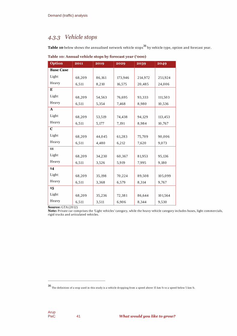
Demand (traffic) analysis
ArupPwC 41 What would you like to grow?
4.3.3 Vehicle stops
Table 10 below shows the annualised network vehicle stops36
by vehicle type, option and forecast year.
Table 10: Annual vehicle stops by forecast year (‘000)
Option 2011 2019 2029 2039 2049
Base Case
Light 68,209 86,161 173,946 214,972 251,924
Heavy 6,511 8,210 16,575 20,485 24,006
E
Light 68,209 54,563 76,695 93,333 111,503
Heavy 6,511 5,354 7,468 8,980 10,536
A
Light 68,209 53,519 74,438 94,129 113,453
Heavy 6,511 5,177 7,191 8,984 10,767
C
Light 68,209 44,045 61,283 75,709 90,006
Heavy 6,511 4,480 6,212 7,620 9,073
11
Light 68,209 34,230 60,367 81,953 95,136
Heavy 6,511 3,526 5,919 7,995 9,180
14
Light 68,209 35,198 70,224 89,508 105,099
Heavy 6,511 3,368 6,579 8,314 9,767
15
Light 68,209 35,236 72,381 86,644 101,564
Heavy 6,511 3,511 6,906 8,344 9,530
Source: GTA (2012)Note: Private car comprises the ‘Light vehicles’ category, while the heavy vehicle category includes buses, light commercials,rigid trucks and articulated vehicles.
36The definition of a stop used in this study is a vehicle dropping from a speed above 15 km/h to a speed below 5 km/h.
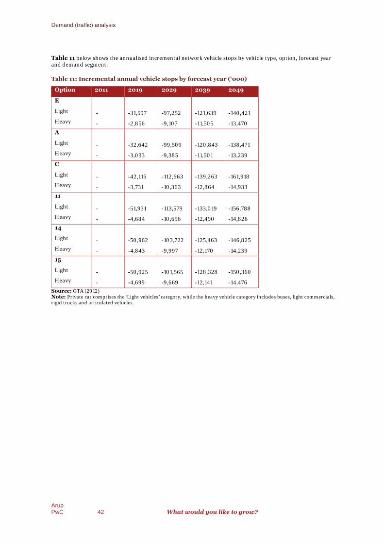
Demand (traffic) analysis
ArupPwC 42 What would you like to grow?
Table 11 below shows the annualised incremental network vehicle stops by vehicle type, option, forecast yearand demand segment.
Table 11: Incremental annual vehicle stops by forecast year (‘000)
Option 2011 2019 2029 2039 2049
E
Light - -31,597 -97,252 -121,639 -140,421
Heavy - -2,856 -9,107 -11,505 -13,470
A
Light - -32,642 -99,509 -120,843 -138,471
Heavy - -3,033 -9,385 -11,501 -13,239
C
Light - -42,115 -112,663 -139,263 -161,918
Heavy - -3,731 -10,363 -12,864 -14,933
11
Light - -51,931 -113,579 -133,019 -156,788
Heavy - -4,684 -10,656 -12,490 -14,826
14
Light - -50,962 -103,722 -125,463 -146,825
Heavy - -4,843 -9,997 -12,170 -14,239
15
Light - -50,925 -101,565 -128,328 -150,360
Heavy - -4,699 -9,669 -12,141 -14,476
Source: GTA (2012)Note: Private car comprises the ‘Light vehicles’ category, while the heavy vehicle category includes buses, light commercials,rigid trucks and articulated vehicles.

Estimating road user and external costs
ArupPwC 43 What would you like to grow?
5 Estimating road user and external costs
This Chapter defines the road user and external costs that are contained in theeconomic evaluation. It also defines the road user cost estimation methodologiesby type and presents the assumptions that are used to calculate the change in roaduser and external costs by route options.
5.1 Definition of road user external costs
The incremental benefits of each route option are measured in terms of savings (reductions) in road user andexternal costs. As identified above in Table 5, these savings arise from a reduction in VHT, VKT, stops and animprovement in average network speeds, compared with the Base Case.
The benefits associated with the route options include:
savings in travel time costs;
savings in vehicle operating costs including stops;
savings in crash costs;
savings in environmental costs; and
residual value of assets.
A summary of the determinants of road user travel costs are shown earlier in Table 5.
5.2 Travel time costs
Annualised incremental VHT from GTA’s traffic forecasts are used to estimate savings in travel time cost withthe route options, relative to the Base Case.
This involves applying an appropriate value of travel time (VOTT) to the annual VHT with the Base Case androute options. The VOTT is sourced from the RMS Economic Analysis Manual, Version 2, 199937, and isreported by vehicle type to the extent to which vehicle type implies trip purpose – i.e. commercial versusprivate vehicle use – and the proportion of the vehicle fleet comprised by each vehicle type.
The RMS Guidelines38 classify Grafton as a rural area for the purposes of economic evaluation.
However, the VOTT used in this analysis uses the urban values presented in the RMS Guidelines, which are inturn, based on the observed concentration of traffic during the peak periods in the study catchment. The VOTTparameter for non-urban areas is more appropriate for road networks characterised by higher speed limits andtravel speeds.
The weighted average VOTT for this evaluation is calculated using data from Tables 7, 8 and 9 of Appendix B ofRMS Economic Analysis Manual – Economic Parameters for 2009, which present urban vehicle composition,occupancy by time of day and value of travel time (urban).
37RMS 1999, RMS Economic Analysis Manual, Version 2, 1999, RMS Corporate Finance and Strategy, Economic Parameters for 2009.
38 RMS Guidelines base categorisation from ABS categorisation in ABS Survey of Motor Vehicle Use (SMVU) Australia 9208.0 p.43 (2008).

Estimating road user and external costs
ArupPwC 44 What would you like to grow?
Vehicle occupancy rates in the RMS Guidelines have been adopted for this study. These are shown below inTable 12.
Table 12: Assumed vehicle occupancies (number of passengers per vehicle)
Hours Private Car Business CarCommercial
Light Heavy
Peak 1.12 1.2 1.3 1.0
Business 1.5 1.4 1.3 1.0
Other 1.97 1.4 1.3 1.0
Source: RMS (1999, 2009 update of Appendix B, Table 8, p.9)
The model results supplied by GTA indicate that the composition of the traffic demand in the peak differs tothe vehicle compositions presented in Table 7 of Appendix B of RMS Economic Analysis Manual – EconomicParameters for 2009. The study specific compositions are adopted in this economic evaluation. These arecompared to the RMS compositions below in Table 13.
Table 13: Study specific vehicle compositions
HoursPrivate
Car
Business
Car
Commercial
Light Heavy
RMS Peak (%) 80.0 5.0 11.0 4.0
Model Peak (%) 88.5 5.5 4.4 1.6
Business 63.0 22.0 10.0 5.0
Other hours 85.0 5.0 7.0 3.0
Source: RMS (1999, 2009 update of Appendix B, Table 7, p.9)
This economic evaluation uses the values of travel time in Table 14 to estimate travel time cost savings.
Table 14: Value of travel time (urban)
Hours
Private
Car
Business
CarCommercial light Commercial heavy
$/person
hour
$/person
hour
Occupant Freight Occupant Freight
$/person
Hour
$/veh.
Hour
$/person
hour
$/veh.
hour
Peak and
Business11.89 38.05 23.31 1.26 24.75 22.13
Other 11.89 11.89 23.31 25.5 11.89 11.89
Source: RMS (1999, 2009 update of Appendix B, Table 9, p.9)
Based on the assumptions identified in Table 12, Table 13 and Table 14, values of travel time used in thisevaluation are:
light vehicles – $22.82/VHT; and
heavy vehicles – $36.07/VHT.
To estimate the change in travel time costs, the VOTT parameters are combined with the VHT output from thetraffic demand forecasts by option.
Table 15 below shows the incremental annual travel time cost for each forecast year and in total over theevaluation period (undiscounted and in present value terms). Negative values indicate cost savings. The totalsare calculated by interpolating values between forecast years.

Estimating road user and external costs
ArupPwC 45 What would you like to grow?
Table 15: Incremental travel time costs by forecast year ($’000), total ($’000) and totaldiscounted (PV$’000)
Option $’000 PV$’000 2011 2019 2029 2039 2049
E
Light -633,543 -133,916 - -9,586 -18,866 -23,985 -28,670
Heavy -105,249 -22,020 - -1,550 -3,068 -3,992 -4,919
A
Light -563,401 -119,618 - -8,371 -17,213 -21,355 -24,823
Heavy -95,337 -19,572 - -1,318 -2,738 -3,457 -4,919
C
Light -655,528 -139,027 - -10,038 -19,646 -24,687 -29,105
Heavy -103,627 -21,792 - -1,531 -3,074 -3,914 -4,693
11
Light -614,628 -133,766 - -10,875 -18,701 -22,266 -26,721
Heavy -99,730 -21,433 - -1,676 -2,991 -3,645 -4,448
14
Light -477,653 -108,029 - -10,020 -14,832 -17,018 -19,280
Heavy -83,121 -18,376 - -1,642 -2,474 -3,010 -3,581
15
Light -494,270 -110,324 - -10,250 -14,574 -18,196 -20,221
Heavy -81,813 -17,844 - -1,572 -2,349 -3,015 -3,580
Source: GTA (2012), PwCNote: Private car comprises the ‘Light vehicles’ category, while the heavy vehicle category includes buses, light commercials,rigid trucks and articulated vehicles.
5.3 Vehicle operating costs
The change in vehicle operating costs (VOC) with the route options is estimated by applying the modelledvehicle compositions, VKT and journey speeds to the freeway model outlined in RMS (2009, Appendix B, p.5).The freeway model is used to ensure that there is no double counting of benefits associated with the reductionin stops, which are estimated explicitly below. The freeway model equation is shown below:
c = C0 + C1V+ C2V2, where:
c = VOC per kilometre;
V = is journey speed (km/hr); and
C0, C1 and C2 are estimated model coefficients linked to vehicle type.
The traffic modelling provided by GTA includes estimates of annual weighted average (across AM and PMpeaks) network speeds for the Base Case (2019) and each option by forecast year. Speeds are provided byvehicle class. However, due to the large proportion of the total number of trips accounted for by privatevehicles, the total network speeds approximate those for ‘light’ vehicles.
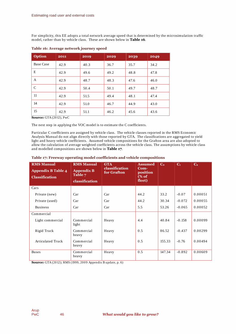
Estimating road user and external costs
ArupPwC 46 What would you like to grow?
For simplicity, this EE adopts a total network average speed that is determined by the microsimulation trafficmodel, rather than by vehicle class. These are shown below in Table 16.
Table 16: Average network journey speed
Option 2011 2019 2029 2039 2049
Base Case 42.9 40.3 36.7 35.7 34.2
E 42.9 49.6 49.2 48.8 47.8
A 42.9 48.7 48.3 47.6 46.0
C 42.9 50.4 50.1 49.7 48.7
11 42.9 51.5 49.4 48.1 47.4
14 42.9 51.0 46.7 44.9 43.0
15 42.9 51.1 46.2 45.6 43.6
Source: GTA (2012), PwC
The next step in applying the VOC model is to estimate the C coefficients.
Particular C coefficients are assigned by vehicle class. The vehicle classes reported in the RMS EconomicAnalysis Manual do not align directly with those reported by GTA. The classifications are aggregated to yieldlight and heavy vehicle coefficients. Assumed vehicle compositions for the Grafton area are also adopted toallow the calculation of average weighted coefficients across the vehicle class. The assumptions by vehicle classand modelled compositions are shown below in Table 17.
Table 17: Freeway operating model coefficients and vehicle compositions
RMS Manual
Appendix B Table 4
Classification
RMS Manual
Appendix BTable 7
classification
GTAclassificationfor Grafton
AssumedCom-position(% offleet)
C0 C1 C2
Cars
Private (new) Car Car 44.2 33.2 -0.07 0.00051
Private (used) Car Car 44.2 30.34 -0.072 0.00055
Business Car Car 5.5 53.26 -0.065 0.00052
Commercial
Light commercial Commerciallight
Heavy 4.4 40.84 -0.158 0.00099
Rigid Truck Commercialheavy
Heavy 0.5 86.52 -0.437 0.00299
Articulated Truck Commercialheavy
Heavy 0.5 155.33 -0.76 0.00494
Buses Commercialheavy
Heavy 0.5 147.34 -0.892 0.00609
Source: GTA (2012); RMS (1999, 2009 Appendix B update, p. 6)

Estimating road user and external costs
ArupPwC 47 What would you like to grow?
The resultant weighted average coefficients are:
C0 = 35;
C1 = -0.08; and
C2 = 0.001
Based on the data presented in Table 16 and Table 17 and vehicle compositions, the appropriate VOCparameters for this analysis are calculated based on the average network speed achieved in each year of theevaluation period.
The unit VOCs estimated from the freeway model are identified below in Table 18.
Table 18: Unit VOC estimated from freeway vehicle operating model ($/VKT)
Option 2011 2019 2029 2039 2049
Base Case 0.3229 0.3237 0.3251 0.3254 0.3261
E 0.3229 0.3211 0.3212 0.3212 0.3215
A 0.3229 0.3213 0.3214 0.3215 0.3220
C 0.3229 0.3209 0.3209 0.3210 0.3213
11 0.3229 0.3206 0.3211 0.3214 0.3216
14 0.3229 0.3207 0.3218 0.3223 0.3228
15 0.3229 0.3207 0.3219 0.3221 0.3227
Source: GTA (2012), (1999, 2009 Appendix B update, p. 6)
The incremental unit VOC is applied to the total VKTs with each of the route options to calculate theincremental VOC for the analysis period. The approach seeks to identify the incremental change in unit VOCas a result of improvements in network speed. Therefore, the incremental change is captured in the unit costand applies to absolute total VKTs travelled with each option, as opposed to the incremental VKTs identifiedabove in Table 9. The incremental VOC are shown below in Table 19.
Table 19: Incremental vehicle operating costs by forecast year ($’000), total ($’000) and totaldiscounted (PV$’000)
Option $’000 PV$’000 2011 2019 2029 2039 2049
E -34,762 -7,455 - -555 -1,041 -1,355 -1,532
A -13,152 -2,860 - -176 -452 -517 -555
C -27,554 -5,944 - -408 -885 -1,054 -1,195
11 -22,012 -5,014 - -431 -737 -778 -915
14 -4,630 -1,009 - -88 -119 -216 -226
15 -7,345 -1,771 - -165 -271 -253 -299
Source: GTA (2012), PwCNote: Private car comprises the ‘Light vehicles’ category, while the heavy vehicle category includes buses, light commercials,rigid trucks and articulated vehicles.
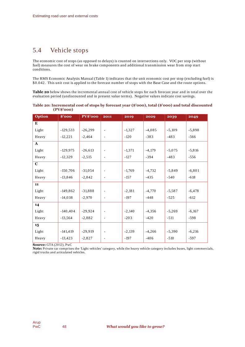
Estimating road user and external costs
ArupPwC 48 What would you like to grow?
5.4 Vehicle stops
The economic cost of stops (as opposed to delays) is counted on intersections only. VOC per stop (withoutfuel) measures the cost of wear on brake components and additional transmission wear from stop startconditions.
The RMS Economic Analysis Manual (Table 1) indicates that the unit economic cost per stop (excluding fuel) is$0.042. This unit cost is applied to the forecast number of stops with the Base Case and the route options.
Table 20 below shows the incremental annual cost of vehicle stops for each forecast year and in total over theevaluation period (undiscounted and in present value terms). Negative values indicate cost savings.
Table 20: Incremental cost of stops by forecast year ($’000), total ($’000) and total discounted(PV$’000)
Option $’000 PV$’000 2011 2019 2029 2039 2049
E
Light -129,533 -26,299 - -1,327 -4,085 -5,109 -5,898
Heavy -12,221 -2,464 - -120 -383 -483 -566
A
Light -129,975 -26,613 - -1,371 -4,179 -5,075 -5,816
Heavy -12,329 -2,515 - -127 -394 -483 -556
C
Light -150,706 -31,054 - -1,769 -4,732 -5,849 -6,801
Heavy -13,846 -2,842 - -157 -435 -540 -618
11
Light -149,862 -31,888 - -2,181 -4,770 -5,587 -6,478
Heavy -14,038 -2,970 - -197 -448 -525 -612
14
Light -140,404 -29,924 - -2,140 -4,356 -5,269 -6,167
Heavy -13,564 -2,882 - -203 -420 -511 -598
15
Light -141,419 -29,919 - -2,139 -4,266 -5,390 -6,216
Heavy -13,423 -2,827 - -197 -406 -510 -597
Source: GTA (2012), PwCNote: Private car comprises the ‘Light vehicles’ category, while the heavy vehicle category includes buses, light commercials,rigid trucks and articulated vehicles.
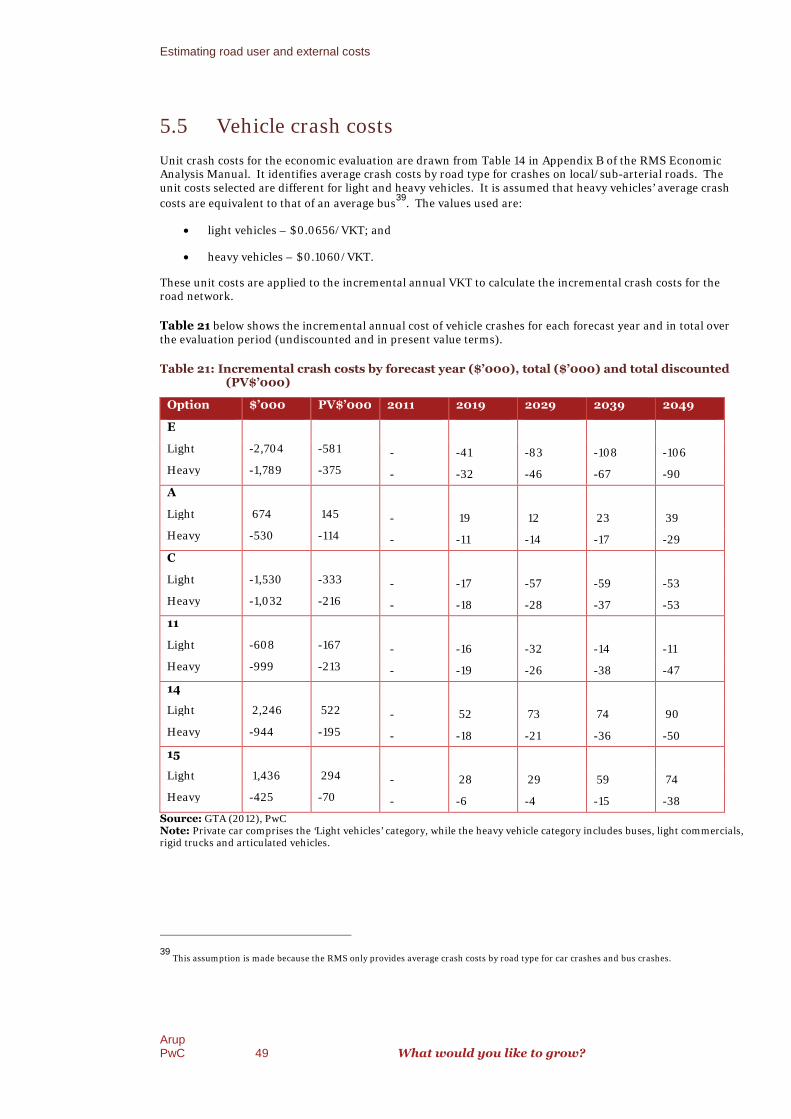
Estimating road user and external costs
ArupPwC 49 What would you like to grow?
5.5 Vehicle crash costs
Unit crash costs for the economic evaluation are drawn from Table 14 in Appendix B of the RMS EconomicAnalysis Manual. It identifies average crash costs by road type for crashes on local/sub-arterial roads. Theunit costs selected are different for light and heavy vehicles. It is assumed that heavy vehicles’ average crash
costs are equivalent to that of an average bus39
. The values used are:
light vehicles – $0.0656/VKT; and
heavy vehicles – $0.1060/VKT.
These unit costs are applied to the incremental annual VKT to calculate the incremental crash costs for theroad network.
Table 21 below shows the incremental annual cost of vehicle crashes for each forecast year and in total overthe evaluation period (undiscounted and in present value terms).
Table 21: Incremental crash costs by forecast year ($’000), total ($’000) and total discounted(PV$’000)
Option $’000 PV$’000 2011 2019 2029 2039 2049
E
Light -2,704 -581 - -41 -83 -108 -106
Heavy -1,789 -375 - -32 -46 -67 -90
A
Light 674 145 - 19 12 23 39
Heavy -530 -114 - -11 -14 -17 -29
C
Light -1,530 -333 - -17 -57 -59 -53
Heavy -1,032 -216 - -18 -28 -37 -53
11
Light -608 -167 - -16 -32 -14 -11
Heavy -999 -213 - -19 -26 -38 -47
14
Light 2,246 522 - 52 73 74 90
Heavy -944 -195 - -18 -21 -36 -50
15
Light 1,436 294 - 28 29 59 74
Heavy -425 -70 - -6 -4 -15 -38
Source: GTA (2012), PwCNote: Private car comprises the ‘Light vehicles’ category, while the heavy vehicle category includes buses, light commercials,rigid trucks and articulated vehicles.
39This assumption is made because the RMS only provides average crash costs by road type for car crashes and bus crashes.
Estimating road user and external costs
ArupPwC 50 What would you like to grow?
5.6 External costs
Road use produces external costs on society in terms of the economic costs of environmental impacts.Therefore, changes in VKT will translate into changes in associated environmental costs. The environmentalunit costs used in this economic evaluation are based on the parameters presented in Appendix B, Table 18 ofthe RMS EAM 2009, and include:
noise;
air pollution;
water pollution;
Greenhouse Gas Emissions (GHG);
nature and landscape; and
urban separation costs.
For an urban road network the RMS manual considers four classes of vehicle for which they provide separateenvironmental externality values:
passenger vehicles;
buses;
light vehicles; and
heavy vehicles.
5.6.1 Passenger vehicles and buses
Environmental unit costs for passenger vehicles are expressed in dollars per VKT in the RMS EconomicAnalysis Manual. The unit costs are directly applied to the change in VKT to estimate the change inenvironmental costs by route option. The average environmental external costs per VKT used primarily forthese vehicles are:
passenger vehicles – $0.0683/VKT; and
buses – $0.5214/VKT.
In order to convert the above environmental cost parameters into annual environmental costs by option, thepassenger vehicle and buses costs per VKT above are applied to the annual VKT for each vehicle type in eachoption.
5.6.2 Freight vehicles
For freight vehicles, the RMS expresses environmental unit costs in cents per tonne kilometre (tkm), whichrequires conversion for application to this economic evaluation. The tkm unit costs are converted to dollarsper VKT using NSW average tonne per trip for the light and heavy vehicle types taken from the latestAustralian Bureau of Statistics “Survey of Motor Vehicle Use”.
The survey provides different average freight loads for ‘Light Commercial’, ‘Heavy Commercial – Rigid’ and‘Heavy Commercial – articulated’ which requires an additional traffic classification step to match this approachwith the approach used in Table 18 of the RMS manual.
A summary of the traffic classification, the assumed vehicle composition, the average load per trip, and thecalculated environmental externality value for each component of traffic is provided in Table 22.

Estimating road user and external costs
ArupPwC 51 What would you like to grow?
Table 22: Calculation assumptions for environmental externality values
ABS Survey of MotorVehicle Use
classification40
RMS ManualAppendix BTable 18classification
Assumedtrafficcomposition(%)
Averagefreight load(tonnes)
Environmentalexternalityvalues per VKT($)
Passenger vehicles Passengervehicles
94.0 n/a 0.0683
Buses Buses 0.5 n/a 0.5214
Light commercial Light Vehicles 4.4 0.00046 0.1479
Heavy commercial – Rigid Heavy Vehicles 0.5 0.00599 0.2265
Heavy commercial –Articulated
Heavy vehicles 0.5 0.02222 0.8401
These calculated results from this approach are expressed in terms of ‘cars’ and ‘heavy vehicles’ (as provided bythe GTA modelling) through appropriate weighting. These values are:
value for cars – $0.0683/VKT; and
value for heavy vehicles – $0.2489/VKT.
These unit costs are applied to the incremental annual VKT to calculate the incremental external costs for theroad network. Table 23 below shows the incremental annual external cost of vehicle for each forecast yearand in total over the evaluation period (undiscounted and in present value terms).
40Australian Bureau of Statistics 2010, Survey of Motor Vehicle Use, Australia, 9208.0 - 12 months ended 31 October 2010.

Estimating road user and external costs
ArupPwC 52 What would you like to grow?
Table 23: Incremental external costs by forecast year ($’000), total ($’000) and totaldiscounted (PV$’000)
Option $’000 PV$’000 2011 2019 2029 2039 2049
E
Light -2,815 -605 - -43 -86 -113 -111
Heavy -4,200 -880 - -75 -109 -156 -212
A
Light 702 151 - 20 12 24 41
Heavy -1,245 -269 - -27 -33 -41 -67
C
Light -1,593 -346 - -17 -59 -62 -55
Heavy -2,422 -508 - -41 -66 -86 -125
11
Light -633 -174 - -17 -33 -15 -11
Heavy -2,346 -500 - -44 -62 -88 -111
14
Light 2,338 544 - 54 76 77 94
Heavy -2,216 -459 - -43 -50 -85 -117
15
Light 1,495 306 - 30 30 62 77
Heavy -999 -164 - -13 -9 -36 -88
Source: GTA (2012), PwCNote: Private car comprises the ‘Light vehicles’ category, while the heavy vehicle category includes buses, light commercials,rigid trucks and articulated vehicles.

Direct infrastructure costs
ArupPwC 53 What would you like to grow?
6 Direct infrastructure costs
6.1 Capital costs
6.1.1 Definitions
Capital cost estimates were provided by Arup’s technical advisor, MacDonald International. The estimates aredefined in terms of the following categories:
project development;
investigation and design;
property acquisition;
public utility adjustments;
construction; and
handover.
The cost estimation approach is detailed in MacDonald International’s Cost Estimates Report41
. The
assumptions which are relevant for the economic evaluation include42
:
costs are in 2012 prices (Quarter 2);
no profit margin was allowed in the construction cost estimates to ensure that values are in real
terms43
;
the indicative cost of the four upgrades with the Base Case (see Section 2.6) is based on measuringthe pavement areas, making allowances based on the length of kerb, and using proportions ofconstruction costs from the current route options. These upgrades would also occur with the routeoption cases. MacDonald International advises that the total cost of the Base Case projects is in theorder of $18 million which includes construction costs, contingency, project development,investigation and design, utilities and handover. Given that the Base Case is not explicitly costed, thecost of Base Case upgrades is wholly deducted from the construction cost component of each routeoption to ensure that construction costs are incremental;
costs are not estimated using a probabilistic approach. However, MacDonald International indicatesthat estimates are equivalent to a P90 estimate; and
MacDonald International disaggregated the construction cost categories by asset type so that residualvalues could be estimated. This process also allocated indirect costs such as contingency, projectmanagement, sponsor costs and insurance across asset type.
41MacDonald International 2012, Main Road 83 – Summerland Way, Additional Crossing of the Clarence River at Grafton: Route Options
Development Report – Technical Paper: Strategic Cost Estimate, August.
42These assumptions are implied in the MacDonald International Technical Paper.
43PwC adjusted the direct infrastructure costs by removing the profit margin identified by MacDonald International.

Direct infrastructure costs
ArupPwC 54 What would you like to grow?
6.1.2 Undiscounted capital costs
The total undiscounted capital costs by option are shown below in Figure 12. The costs exclude a 9 per centprofit margin and are incremental to the upgrade works that would take place with the Base Case. The figureshows that Route Option 14 and Route Option 15 have the highest cost, while Route Options E and 11 have thelowest.
The capital costs are in the range of $170-$300 million.
Figure 12: Undiscounted total capital costs by option
0
50,000,000
100,000,000
150,000,000
200,000,000
250,000,000
300,000,000
E A C 11 14 15
$(2
012,
real)
Option
Source: MacDonald International (2012)Note: Excludes 9 per cent profit margin and Base Case upgrade costs.
The range of total cost by option is relatively wide.
Figure 13 presents the total costs by option as an Index, where an index value of 1 indicates the lowest costoption. Figure 13 indicates that Route Option 11 has the lowest cost, with the total cost of Route Options 14and 15 being around 50 per cent and 70 per cent higher than Route Option 11, respectively.
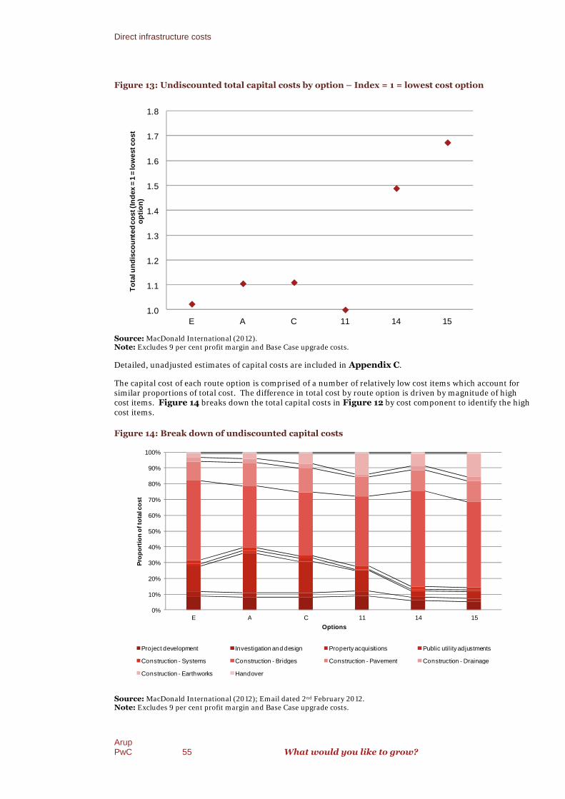
Direct infrastructure costs
ArupPwC 55 What would you like to grow?
Figure 13: Undiscounted total capital costs by option – Index = 1 = lowest cost option
1.0
1.1
1.2
1.3
1.4
1.5
1.6
1.7
1.8
E A C 11 14 15
To
talu
nd
isco
unte
dco
st(I
nd
ex
=1
=lo
westco
st
op
tio
n)
Source: MacDonald International (2012).Note: Excludes 9 per cent profit margin and Base Case upgrade costs.
Detailed, unadjusted estimates of capital costs are included in Appendix C.
The capital cost of each route option is comprised of a number of relatively low cost items which account forsimilar proportions of total cost. The difference in total cost by route option is driven by magnitude of highcost items. Figure 14 breaks down the total capital costs in Figure 12 by cost component to identify the highcost items.
Figure 14: Break down of undiscounted capital costs
0%
10%
20%
30%
40%
50%
60%
70%
80%
90%
100%
E A C 11 14 15
Pro
po
rtio
no
fto
talc
ost
Options
Project development Investigation and design Propertyacquisitions Public utilityadjustments
Construction - Systems Construction - Bridges Construction - Pavement Construction - Drainage
Construction - Earthworks Handover
Source: MacDonald International (2012); Email dated 2nd February 2012.Note: Excludes 9 per cent profit margin and Base Case upgrade costs.
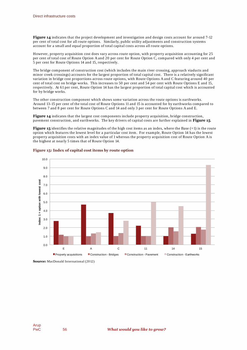
Direct infrastructure costs
ArupPwC 56 What would you like to grow?
Figure 14 indicates that the project development and investigation and design costs account for around 7-12per cent of total cost for all route options. Similarly, public utility adjustments and construction systemsaccount for a small and equal proportion of total capital costs across all route options.
However, property acquisition cost does vary across route option, with property acquisition accounting for 25per cent of total cost of Route Option A and 20 per cent for Route Option C, compared with only 4 per cent and5 per cent for Route Options 14 and 15, respectively.
The bridge component of construction cost (which includes the main river crossing, approach viaducts andminor creek crossings) accounts for the largest proportion of total capital cost. There is a relatively significantvariation in bridge cost proportions across route options, with Route Options A and C featuring around 40 percent of total cost on bridge works. This increases to 50 per cent and 54 per cent with Route Options E and 15,respectively. At 61 per cent, Route Option 14 has the largest proportion of total capital cost which is accountedfor by bridge works.
The other construction component which shows some variation across the route options is earthworks.Around 13-15 per cent of the total cost of Route Options 11 and 15 is accounted for by earthworks compared tobetween 7 and 8 per cent for Route Options C and 14 and only 3 per cent for Route Options A and E.
Figure 14 indicates that the largest cost components include property acquisition, bridge construction,pavement construction, and earthworks. The key drivers of capital costs are further explained in Figure 15.
Figure 15 identifies the relative magnitudes of the high cost items as an index, where the Base (=1) is the routeoption which features the lowest level for a particular cost item. For example, Route Option 14 has the lowestproperty acquisition costs with an index value of 1 whereas the property acquisition cost of Route Option A isthe highest at nearly 5 times that of Route Option 14.
Figure 15: Index of capital cost items by route option
0.0
1.0
2.0
3.0
4.0
5.0
6.0
7.0
8.0
9.0
10.0
E A C 11 14 15
Ind
ex:
1=
op
tio
nw
ith
low
est
co
st
Property acquisitions Construction - Bridges Construction - Pavement Construction - Earthworks
Source: MacDonald International (2012)

Direct infrastructure costs
ArupPwC 57 What would you like to grow?
6.1.3 Capital cost cash flow profile
Arup defined the likely cash flow profiles of capital costs by item and route option. This is used to distributethe capital costs over time, based on when expenditure is expected to occur. The information provided by Arupalso indicates that the construction period, including pre-construction activities, commences in 2011 and endsin 2019 with handover. The handover accounts for a small cost and is not construction related. The first fullyear of operation of the additional crossing of the Clarence River at Grafton is assumed to be 2019/20. Thecashflow profiles are applied to the total undiscounted infrastructure costs by route option to generate thecashflows shown below in Figure 16.
Figure 16: Capital cost cash flows by route option
2011 2012 2013 2014 2015 2016 2017 2018 2019
E 5,192 10,384 21,364 36,967 65,220 103,174 141,127 179,081 180,493
A 5,192 10,384 25,348 49,239 85,183 121,339 157,496 193,653 195,006
C 5,192 10,384 23,320 43,757 77,215 116,277 155,338 194,400 195,839
11 5,192 10,384 20,186 32,724 58,235 97,155 136,076 174,996 176,424
14 5,192 10,384 17,664 25,903 56,756 124,599 192,441 260,284 262,663
15 5,192 10,384 18,276 27,774 62,797 139,371 215,946 292,521 295,186
-
50,000
100,000
150,000
200,000
250,000
300,000
$'0
00
cu
mu
lati
ve
Source: MacDonald International (2012), Arup (2012, email dated 13th February 2012)
The streamed costs are discounted at a real discount rate of 7 per cent and expressed in present value terms.These are shown below in Table 24. These costs do not include residual values.

Direct infrastructure costs
ArupPwC 58 What would you like to grow?
Table 24: Incremental capital costs by route option
Route option Undiscounted total
($’000, 2012 m)
Discounted total
(PV$’000)
Option E 180,493 127,373
Option A 195,006 139,037
Option C 195,839 138,456
Option 11 176,424 123,936
Option 14 262,663 177,040
Option 15 295,186 197,967
Source: Arup (2012), MacDonald International (2012).
Detailed capital cost cashflows are provided in Appendix D.
6.2 Recurrent costs
Recurrent, or variable, costs are defined as those costs that recur, as opposed to capital, or fixed, costs, whichare concentrated at the beginning of a project's life.
It has been assumed that recurrent costs are the same for the Base Case as for bridge route options. Whilenewer roads under the route options are likely to require lower levels or frequency of maintenance as olderroads, the route options are expected to result in additional maintenance from additional road surfaces. Thishas been assumed to result in recurrent costs for the route options equalling the Base Case, i.e. incrementalrecurrent costs are negligible.
6.3 Residual (terminal) values
This economic evaluation includes the residual values of road infrastructure assets.
The residual value reflects the fact that some assets have economic lives which extend beyond the evaluationperiod. Residual values are entered in the last year of the evaluation period (2048/49) to represent the unusedportion of assets that have lives greater than the evaluation period.
The economic lives, by asset class, adopted in this economic evaluation are shown below in Table 25.
It should be noted that land does not depreciate and hence, its full value is retained at the end of the evaluationperiod.

Direct infrastructure costs
ArupPwC 59 What would you like to grow?
Table 25: Economic lives by asset type
Asset type Economic Life1 Economic LifeRemaining in 2048/495
Systems2 25 -
Bridges3 120 90
Pavement 50 20
Drainage4 110 80
Earthworks 125 95
Property Infinite Full
Source: Australian Transport Council 2006, National Guidelines for Transport Systems Management in Australia, Volume4, Urban Transport, p. 44.Notes:1 The ‘systems’ construction component is assumed to have an economic life similar to that for traffic lights.2In some cases, the ATC Guidelines present a range of economic lives for a particular type of asset. The analysis adopts amid-point value of the range.3Refers to the economic life of a concrete bridge.4Refers to the economic life of culverts.5Assumes that depreciation of all assets commences from the first full year of operation.
The residual values are calculated by applying straight-line depreciation. Depreciation of assets for each routeoption is assumed to commence in 2019/20. Given that the period of analysis is for a further 30 years from thefirst full year of operation, the residual value is identified for 2048/49. These residual values are shown belowin Table 26.
Table 26: Residual value by asset type ($000, undiscounted, 2048/49)
Asset Type Route Option
E A C 11 14 15
Systems - - - - - -
Bridges 68,144 57,128 58,915 58,380 119,243 120,396
Pavement 8,741 11,570 12,052 8,782 13,825 15,554
Drainage 3,346 3,506 3,913 2,177 5,027 5,801
Earthworks 3,496 5,129 9,814 17,444 15,761 32,584
Property 28,938 48,861 38,719 23,049 10,440 13,499
Total 112,665 126,194 123,413 109,833 164,296 187,834
Source: MacDonald International (2012), PwC

Results
ArupPwC 60 What would you like to grow?
7 Results
This Chapter of the report presents discounted total direct infrastructure, road userand external costs by route option. These incremental costs are combined toproduce the measures of economic performance including BCR and NPV. It alsopresents the results of sensitivity analysis undertaken on a selection of keyassumptions.
7.1 RUCBA results
The changes in direct infrastructure, road user and external costs detailed in Chapter 5 and Chapter 6 arepresented below in Table 27. Positive values associated with the direct infrastructure cost componentsindicate increases compared with the Base Case whereas positive values with the road user and external costcomponents refer to savings (or cost reductions).
The results indicate that all route options generate significant savings in travel time cost, between PV$120 -$160m. Route Options E, C and 11 generate the highest travel time cost savings. Savings in travel time costsalso account for the largest proportion of total present value benefits at around 80 per cent for each routeoption.
The next largest benefit component involves the reduction in economic costs associated with a reduction invehicle stops. This benefit line item accounts for between 15 and 20 per cent of total present value benefits.
Route Options E, C and 11 generate similar levels of total present value benefit.
Table 27: Discounted incremental infrastructure, road user and external costs by route option($’000)
Cost/Benefit Item PV$’000
E A C 11 14 15
Direct Infrastructure Cost
Capital 127,373 139,037 138,456 123,936 177,040 197,967
Operating and maintenance - - - - - -
Residual -8,050 -9,017 -8,819 -7,848 -11,740 -13,422
Total DirectInfrastructure Cost 119,322 130,020 129,638 116,088 165,300 184,545
Road User Cost (savings)
Travel time cost 155,936 139,190 160,819 155,199 126,404 128,168
Vehicle operating cost 7,455 2,860 5,944 5,014 1,009 1,771
Stop cost 28,763 29,128 33,895 34,858 32,805 32,746
Crash cost 956 -31 549 380 -327 -224
Total Road User Cost(savings) 193,110 171,147 201,208 195,451 159,892 162,461
External Cost (Savings)
Environmental cost 1,485 117 855 674 -85 -142
Total External Cost(savings) 1,485 117 855 674 -85 -142
Total Road User andExternal Cost Savings 194,595 171,264 202,062 196,125 159,807 162,319

Results
ArupPwC 61 What would you like to grow?
The detailed streams of road user and external costs are shown in Appendix E.
Table 28 below combines the data in Table 27 to produce BCRs and NPVs for each route option.
The results indicate that for Route Options E, A, C and 11 the road user and external benefits would appreciablyexceed the capital cost, but for Route Options 14 and 15 the benefits would be marginally lower than the cost.
Table 28: Measures of economic performance by route option
Performance Measure PV$’000
E A C 11 14 15
Net Present Value 75,272 41,244 72,424 80,037 -5,493 -22,226
Benefit Cost Ratio 1.6 1.3 1.6 1.7 1.0 0.9
7.2 Sensitivity analyses
This section presents a range of sensitivity analyses. Sensitivity analyses assess the robustness of the coreresults (see Table 28) with respect to changes in key parameters and assumptions.
7.2.1 Alternate discount rates
Table 29 and Table 30 present the results of the core analysis under alternative discount rates of 4 per centand 10 per cent, respectively.
Table 29: Alternative discount rates – 4 per cent
Performance Measure PV$’000
E A C 11 14 15
Net Present Value 235,645 182,523 238,349 236,439 113,534 99,179
Benefit Cost Ratio 2.9 2.4 2.8 2.9 1.6 1.5
Table 30: Alternative discount rates – 10 per cent
Performance Measure PV$’000
E A C 11 14 15
Net Present Value 5,762 -18,108 842 11,367 -51,189 -66,941
Benefit Cost Ratio 1.1 0.8 1.0 1.1 0.6 0.6
The results of the sensitivity analysis show a significant increase in NPV and BCR values for all options when adiscount rate of 4 per cent is adopted, and the road user and external benefits would appreciably exceed thecapital cost for all route options including Options 14 and 15.
Using a discount rate of 10 per cent, the road user and external benefits reduce significantly. For RouteOptions E, C and 11 the road user and external benefits slightly exceed the capital cost, but for Route OptionsA, 14 and 15 the benefits would be marginally lower than the cost.
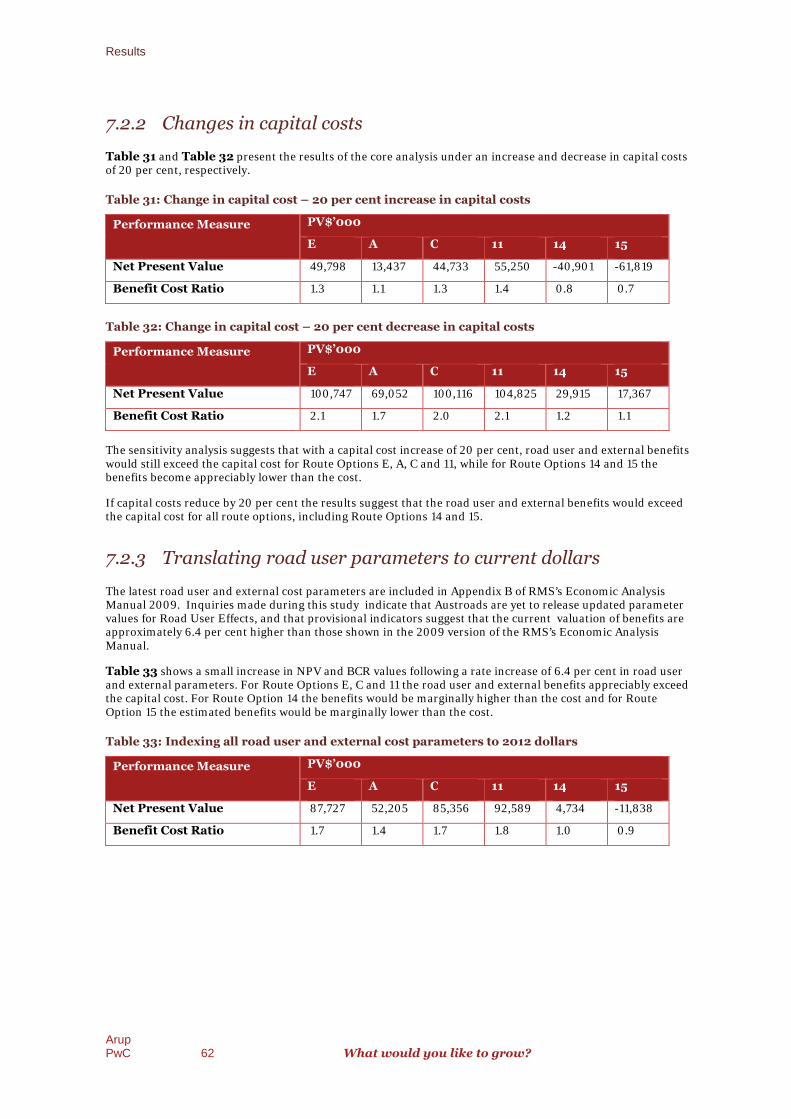
Results
ArupPwC 62 What would you like to grow?
7.2.2 Changes in capital costs
Table 31 and Table 32 present the results of the core analysis under an increase and decrease in capital costsof 20 per cent, respectively.
Table 31: Change in capital cost – 20 per cent increase in capital costs
Performance Measure PV$’000
E A C 11 14 15
Net Present Value 49,798 13,437 44,733 55,250 -40,901 -61,819
Benefit Cost Ratio 1.3 1.1 1.3 1.4 0.8 0.7
Table 32: Change in capital cost – 20 per cent decrease in capital costs
Performance Measure PV$’000
E A C 11 14 15
Net Present Value 100,747 69,052 100,116 104,825 29,915 17,367
Benefit Cost Ratio 2.1 1.7 2.0 2.1 1.2 1.1
The sensitivity analysis suggests that with a capital cost increase of 20 per cent, road user and external benefitswould still exceed the capital cost for Route Options E, A, C and 11, while for Route Options 14 and 15 thebenefits become appreciably lower than the cost.
If capital costs reduce by 20 per cent the results suggest that the road user and external benefits would exceedthe capital cost for all route options, including Route Options 14 and 15.
7.2.3 Translating road user parameters to current dollars
The latest road user and external cost parameters are included in Appendix B of RMS’s Economic AnalysisManual 2009. Inquiries made during this study indicate that Austroads are yet to release updated parametervalues for Road User Effects, and that provisional indicators suggest that the current valuation of benefits areapproximately 6.4 per cent higher than those shown in the 2009 version of the RMS’s Economic AnalysisManual.
Table 33 shows a small increase in NPV and BCR values following a rate increase of 6.4 per cent in road userand external parameters. For Route Options E, C and 11 the road user and external benefits appreciably exceedthe capital cost. For Route Option 14 the benefits would be marginally higher than the cost and for RouteOption 15 the estimated benefits would be marginally lower than the cost.
Table 33: Indexing all road user and external cost parameters to 2012 dollars
Performance Measure PV$’000
E A C 11 14 15
Net Present Value 87,727 52,205 85,356 92,589 4,734 -11,838
Benefit Cost Ratio 1.7 1.4 1.7 1.8 1.0 0.9
Results
ArupPwC 63 What would you like to grow?
7.2.4 Impacts of lower road user and external benefits
Traffic forecasts under various land use scenarios were not supplied for this economic evaluation. The rate oftraffic growth directly impacts on the road user and external cost savings in a particular year. However, therelationship between population and traffic growth is not linear.
This sensitivity analysis undertakes a coarse assessment of the robustness of the results to changes inpopulation and traffic growth by assessing the impacts of a conservative reduction in total present valuebenefits of 30 per cent.
Table 34 shows an appreciable decrease in the NPV and BCR values following a 30 per cent reduction in totalpresent value benefits. For Route Options E, C and 11 the road user and external benefits slightly exceed thecapital cost. For Route Option A the benefits would be slightly lower than the cost and for Route Options 14and 15 the estimated benefits would be appreciably lower than the cost.
Table 34: 30 per cent decrease in present value benefits
Performance Measure PV$’000
E A C 11 14 15
Net Present Value 16,894 -10,135 11,806 21,200 -53,435 -70,922
Benefit Cost Ratio 1.1 0.9 1.1 1.2 0.7 0.6

Conclusions
ArupPwC 64 What would you like to grow?
8 Conclusions
The comparative BCR and NPV results indicate that for Route Options E, A, C and 11, the road user andexternal benefits would appreciably exceed the capital cost, but for Route Options 14 and 15 the benefits wouldbe marginally lower than the cost.
With a BCR of 1.7 and the highest NPV, Route Option 11 performs the best overall. While the road user costsavings with Route Option 11 are marginally lower than with Route Option C, Route Option 11 performs betterdue to a lower capital cost compared with Route Option C.
The performance of the next best Route Options E and C are similar and only marginally behind Route Option11. Route Option C generates higher road user cost savings than Route Option E but this is offset by a highercapital cost.
Route Option A performs does not perform as well as Route Options E, C and 11 because the road user costsavings are lower with Route Option A and it has a comparatively high capital cost.
Route Options 14 and 15 are the worst performing options since they generate the lowest road user cost savingswhile their capital costs are highest.

ArupPwC 65 What would you like to grow?
Appendices
Appendix A Grafton Bridge 66
Appendix B Traffic modelling study area 67
Appendix C Unadjusted capital cost estimates 68
Appendix D Capital cost cashflows by route option 74
Appendix E Detailed road user and external cost profiles 80

ArupPwC 66 What would you like to grow?
Appendix A Grafton Bridge
Figure A 1: The existing Grafton Bridge
Source: Arup (2012, p. 23)
Traffic modelling study area
ArupPwC 67 What would you like to grow?
Appendix B Traffic modelling study area
Figure B 1: Definition of traffic modelling study area
Source: GTA (2012, p.9)

Unadjusted capital cost estimates
ArupPwC 68 What would you like to grow?
Appendix C Unadjusted capital cost estimates
Figure C 1: Capital cost estimate: Route Option E
Source: MacDonald International (2012)

Unadjusted capital cost estimates
ArupPwC 69
Figure C 2: Capital cost estimate:
Source: MacDonald International (2012)
Unadjusted capital cost estimates
What would you like to grow?
: Capital cost estimate: Route Option A
International (2012)
at would you like to grow?

Unadjusted capital cost estimates
ArupPwC 70
Figure C 3: Capital cost estimate:
Source: MacDonald International (2012)
What would you like to grow?
: Capital cost estimate: Route Option C
International (2012)

Unadjusted capital cost estimates
ArupPwC 71
Figure C 4: Capital cost estimate:
Source: MacDonald International (2012)
Unadjusted capital cost estimates
What would you like to grow?
: Capital cost estimate: Route Option 11
International (2012)
at would you like to grow?

Unadjusted capital cost estimates
ArupPwC 72
Figure C 5: Capital cost estimate:
Source: MacDonald International (2012)
What would you like to grow?
imate: Route Option 14
International (2012)

Unadjusted capital cost estimates
ArupPwC 73
Figure C 6: Capital cost estimate:
Source: MacDonald International (2012)
Unadjusted capital cost estimates
What would you like to grow?
: Capital cost estimate: Route Option 15
International (2012)
at would you like to grow?

Capital cost cashflows by route option
ArupPwC 74 What would you like to grow?
Appendix D Capital cost cashflows by route option
Figure D 1: Capital cost cashflows – Route Option E
Opt ion Capit a l Cost s 0 1 2 3 4 5 6 7 8
T ot al ($ m ) PV ($ m ) 2011 2012 2013 2014 2015 2016 2017 2018 2019
Ca pex a s per Cost In pu t Page (i.e. $ m real , a dju st ed t o exclu de 9% profit m a rgin a n d Base Ca se u pgrade cost s)
Pr oject dev elopm en t 12,461 15,054 4 ,1 5 4 4 ,1 5 4 4 ,1 5 4 - - - - - -
Con tin g en cy 3,115 3,764 1 ,03 8 1 ,03 8 1 ,0 3 8 - - - - - -
In v est iga t ion a n d desig n 3,980 2,937 - - - 1 ,9 9 0 1 ,9 9 0 - - - -
Con tin g en cy 1,592 1,175 - - - 7 9 6 7 9 6 - - - -
Pr oper t y a cqu isit ion s 18,436 13,893 - - 3 ,6 8 7 7 ,3 7 4 7 ,3 7 4 - - - -
Con tin g en cy 10,502 7,915 - - 2 ,1 00 4 ,2 01 4 ,2 01 - - - -
Pu blic u tilit y a dju stm en t s 1,658 1,224 - - - 8 2 9 8 2 9 - - - -
Con tin g en cy 824 608 - - - 4 1 2 4 1 2 - - - -
Con str u ct ion - Sy stem s 3,263 2,064 - - - - 3 2 6 9 7 9 9 7 9 9 7 9 -
Con tin g en cy 1,338 846 - - - - 1 3 4 4 0 1 4 0 1 4 0 1 -
Con str u ct ion - Br idg es 64,438 40,766 - - - - 6 ,4 4 4 1 9 ,3 3 2 1 9 ,3 3 2 1 9 ,3 3 2 -
Con tin g en cy 26,420 16,714 - - - - 2 ,6 4 2 7 ,9 2 6 7 ,9 2 6 7 ,9 2 6 -
Con str u ct ion - Pa v em en t 15,498 9,804 - - - - 1 ,5 5 0 4 ,6 4 9 4 ,6 4 9 4 ,6 4 9 -
Con tin g en cy 6,354 4,020 - - - - 6 3 5 1 ,9 06 1 ,9 06 1 ,9 06 -
Con str u ct ion - Dr a in a g e 3,263 2,064 - - - - 3 2 6 9 7 9 9 7 9 9 7 9 -
Con tin g en cy 1,338 846 - - - - 1 3 4 4 0 1 4 0 1 4 0 1 -
Con str u ct ion - Ea r th w or ks 3,263 2,064 - - - - 3 2 6 9 7 9 9 7 9 9 7 9 -
Con tin g en cy 1,338 846 - - - - 1 3 4 4 0 1 4 0 1 4 0 1 -
Ha n dov er 1,009 549 - - - - - - - - 1 ,00 9
Con tin g en cy 404 220 - - - - - - - - 4 04
T ot al (excl. residu al) 180,493 127,373 5,192 5,192 10,980 15,603 28,254 37,953 37,953 37,953 1,412
Residu a l - - 8,050 - - - - - - - - -
T ot al (in cl. residu al) 119,322 5,192 5,192 10,980 15,603 28,254 37,953 37,953 37,953 1,412
Option E
Source: MacDonald International (2012); Arup Email dated 2nd February 2012.

Capital cost cashflows by route option
ArupPwC 75 What would you like to grow?
Figure D 2: Capital cost cashflows – Route Option A
Opt ion Ca pit a l Cost s 0 1 2 3 4 5 6 7 8
T ot al ($ m ) PV ($ m ) 2011 2012 2013 2014 2015 2016 2017 2018 2019
Ca pex as per Cost In pu t Pa ge (i.e. $ m r ea l, a dju st ed t o exclu de 9% profit m a rgin an d Ba se Ca se u pgra de cost s)
Pr oject dev elopm en t 12,461 15,054 4 ,1 5 4 4 ,1 5 4 4 ,1 5 4 - - - - - -
Con t in g en cy 3,115 3,764 1 ,03 8 1 ,03 8 1 ,03 8 - - - - - -
In v est ig a t ion a n d desig n 3,980 2,937 - - - 1 ,9 9 0 1 ,9 9 0 - - - -
Con t in g en cy 1,592 1,175 - - - 7 9 6 7 9 6 - - - -
Pr oper ty a cqu isit ion s 31,550 23,776 - - 6 ,3 1 0 1 2 ,6 2 0 1 2 ,6 2 0 - - - -
Con t in g en cy 17,311 13,046 - - 3 ,4 6 2 6 ,9 2 5 6 ,9 2 5 - - - -
Pu blic u t ility a dju stm en ts 2,085 1,539 - - - 1 ,04 2 1 ,04 2 - - - -
Con t in g en cy 1,036 764 - - - 5 1 8 5 1 8 - - - -
Con str u ct ion - Sy stem s 2,735 1,730 - - - - 2 7 4 8 2 1 8 2 1 8 2 1 -
Con tin g en cy 1,121 709 - - - - 1 1 2 3 3 6 3 3 6 3 3 6 -
Con str u ct ion - Br idg es 54,021 34,175 - - - - 5 ,4 02 1 6 ,2 06 1 6 ,2 06 1 6 ,2 06 -
Con tin g en cy 22,149 14,012 - - - - 2 ,2 1 5 6 ,6 4 5 6 ,6 4 5 6 ,6 4 5 -
Con str u ct ion - Pa v em en t 20,514 12,978 - - - - 2 ,05 1 6 ,1 5 4 6 ,1 5 4 6 ,1 5 4 -
Con tin g en cy 8,411 5,321 - - - - 8 4 1 2 ,5 2 3 2 ,5 2 3 2 ,5 2 3 -
Con str u ct ion - Dr a in a g e 3,419 2,163 - - - - 3 4 2 1 ,02 6 1 ,02 6 1 ,02 6 -
Con tin g en cy 1,402 887 - - - - 1 4 0 4 2 1 4 2 1 4 2 1 -
Con str u ct ion - Ea r th w or ks 4,787 3,028 - - - - 4 7 9 1 ,4 3 6 1 ,4 3 6 1 ,4 3 6 -
Con tin g en cy 1,963 1,242 - - - - 1 9 6 5 8 9 5 89 5 8 9 -
Ha n dov er 967 526 - - - - - - - - 9 6 7
Con tin g en cy 387 210 - - - - - - - - 3 8 7
T ot al (Excl. Residu a l) 195,006 139,037 5,192 5,192 14,964 23,891 35,943 36,157 36,157 36,157 1,353
Residu a l - - 9,017 - - - - - - - - -
T ot a l (Incl. Residu a l) 130,020 5,192 5,192 14,964 23,891 35,943 36,157 36,157 36,157 1,353
Option A
Source: MacDonald International (2012); Arup Email dated 2nd February 2012.

Capital cost cashflows by route option
ArupPwC 76 What would you like to grow?
Figure D 3: Capital cost cashflows – Route Option C
Opt ion Ca pit a l Cost s 0 1 2 3 4 5 6 7 8
T ot al ($ m ) PV ($ m ) 2011 2012 2013 2014 2015 2016 2017 2018 2019
Ca pex a s per Cost Inpu t Pa ge (i.e. $ m real , a dju st ed t o exclu de 9% profit m a rgin a nd Base Ca se u pgra de cost s)
Pr oject dev elopm en t 12,461 15,054 4 ,1 5 4 4 ,1 5 4 4 ,1 5 4 - - - - - -
Con tin g en cy 3,115 3,764 1 ,0 3 8 1 ,03 8 1 ,03 8 - - - - - -
In v est ig a t ion a n d desig n 3,980 2,937 - - - 1 ,9 9 0 1 ,9 9 0 - - - -
Con tin g en cy 1,592 1,175 - - - 7 9 6 7 9 6 - - - -
Pr oper ty a cqu isit ion s 25,430 19,165 - - 5 ,0 8 6 1 0 ,1 7 2 1 0 ,1 7 2 - - - -
Con tin g en cy 13,289 10,014 - - 2 ,6 5 8 5 ,3 1 5 5 ,3 1 5 - - - -
Pu blic u t ility a dju stm en ts 2,891 2,133 - - - 1 ,4 4 5 1 ,4 4 5 - - - -
Con tin g en cy 1,436 1,060 - - - 7 1 8 7 1 8 - - - -
Con str u ct ion - Sy stem s 2,273 1,438 - - - - 2 2 7 6 82 6 82 6 8 2 -
Con tin g en cy 955 604 - - - - 9 5 2 86 2 86 2 8 6 -
Con str u ct ion - Br idg es 55,320 34,997 - - - - 5 ,5 3 2 1 6 ,5 9 6 1 6 ,5 9 6 1 6 ,5 9 6 -
Con tin g en cy 23,234 14,699 - - - - 2 ,3 2 3 6 ,9 7 0 6 ,9 7 0 6 ,9 7 0 -
Con str u ct ion - Pa v em en t 21,218 13,423 - - - - 2 ,1 2 2 6 ,3 6 6 6 ,3 6 6 6 ,3 6 6 -
Con tin g en cy 8,912 5,638 - - - - 89 1 2 ,6 7 4 2 ,6 7 4 2 ,6 7 4 -
Con str u ct ion - Dr a in a g e 3,789 2,397 - - - - 3 7 9 1 ,1 3 7 1 ,1 3 7 1 ,1 3 7 -
Con tin g en cy 1,591 1,007 - - - - 1 5 9 4 7 7 4 7 7 4 7 7 -
Con str u ct ion - Ea r th w or ks 9,094 5,753 - - - - 9 0 9 2 ,7 2 8 2 ,7 2 8 2 ,7 2 8 -
Con tin g en cy 3,819 2,416 - - - - 3 8 2 1 ,1 4 6 1 ,1 4 6 1 ,1 4 6 -
Ha n dov er 1,028 559 - - - - - - - - 1 ,02 8
Con tin g en cy 411 224 - - - - - - - - 4 1 1
T ot al (excl. residu a l) 195,839 138,456 5,192 5,192 12,936 20,437 33,458 39,062 39,062 39,062 1,439
Residu a l - - 8,819 - - - - - - - - -
T ot al (In cl. residu a l) 129,638 5,192 5,192 12,936 20,437 33,458 39,062 39,062 39,062 1,439
Option C
Source: MacDonald International (2012); Arup Email dated 2nd February 2012.

Capital cost cashflows by route option
ArupPwC 77 What would you like to grow?
Figure D 4: Capital cost cashflows – Route Option 11
Opt ion Capit a l Cost s 0 1 2 3 4 5 6 7 8
T ot a l ($ m ) PV ($ m ) 2011 2012 2013 2014 2015 2016 2017 2018 2019
Capex a s per Cost Inpu t Pa ge (i.e. $ m real , adju st ed t o exclu de 9% profit m argin a nd Ba se Case u pgrade cost s)
Pr oject dev elopm en t 12,461 15,054 4 ,1 5 4 4 ,1 5 4 4 ,1 5 4 - - - - - -
Con tin g en cy 3,115 3,764 1 ,0 3 8 1 ,0 3 8 1 ,03 8 - - - - - -
In v estig a tion a n d desig n 3,980 2,937 - - - 1 ,9 9 0 1 ,9 9 0 - - - -
Con tin g en cy 1,592 1,175 - - - 7 9 6 7 9 6 - - - -
Pr oper ty acqu isit ion s 14,816 11,165 - - 2 ,9 6 3 5 ,9 2 6 5 ,9 2 6 - - - -
Con tin g en cy 8,233 6,205 - - 1 ,6 4 7 3 ,2 9 3 3 ,2 9 3 - - - -
Pu blic u tilit y a dju st m en ts 711 525 - - - 3 5 5 3 5 5 - - - -
Con tin g en cy 353 261 - - - 1 7 7 1 7 7 - - - -
Con str u ct ion - Sy st em s 2,811 1,778 - - - - 2 8 1 8 4 3 8 4 3 8 4 3 -
Con tin g en cy 1,181 747 - - - - 1 1 8 3 5 4 3 5 4 3 5 4 -
Con str u ct ion - Br idg es 54,817 34,679 - - - - 5 ,4 8 2 1 6 ,4 4 5 1 6 ,4 4 5 1 6 ,4 4 5 -
Con tin g en cy 23,023 14,565 - - - - 2 ,3 02 6 ,9 07 6 ,9 0 7 6 ,9 07 -
Con str u ct ion - Pa v em en t 15,461 9,781 - - - - 1 ,5 4 6 4 ,6 3 8 4 ,6 3 8 4 ,6 3 8 -
Con tin g en cy 6,494 4,108 - - - - 6 4 9 1 ,9 4 8 1 ,9 4 8 1 ,9 4 8 -
Con str u ct ion - Dr a in a g e 2,108 1,334 - - - - 2 1 1 6 3 3 6 3 3 6 3 3 -
Con tin g en cy 886 560 - - - - 8 9 2 6 6 2 6 6 2 6 6 -
Con str u ct ion - Ea r t h w or ks 16,164 10,226 - - - - 1 ,6 1 6 4 ,8 4 9 4 ,8 4 9 4 ,8 4 9 -
Con tin g en cy 6,789 4,295 - - - - 6 7 9 2 ,0 3 7 2 ,03 7 2 ,0 3 7 -
Ha n dov er 1,024 557 - - - - - - - - 1 ,0 2 4
Con tin g en cy 404 220 - - - - - - - - 4 04
Tot a l (excl. r esidu al) 176,424 123,936 5,192 5,192 9,802 12,538 25,511 38,920 38,920 38,920 1,429
Residu al - - 7,848 - - - - - - - - -
T ot al (In cl. residu al) 116,088 5,192 5,192 9,802 12,538 25,511 38,920 38,920 38,920 1,429
Option 11
Source: MacDonald International (2012); Arup Email dated 2nd February 2012.

Capital cost cashflows by route option
ArupPwC 78 What would you like to grow?
Figure D 5: Capital cost cashflows – Route Option 14
Opt ion Ca pit a l Cost s 0 1 2 3 4 5 6 7 8
T ot a l ($ m ) PV ($ m ) 2011 2012 2013 2014 2015 2016 2017 2018 2019
Capex a s per Cost In pu t Pa ge (i.e. $ m rea l, a dju st ed t o exclu de 9% profit m a rgin a nd Base Ca se u pgr ade cost s)
Pr oject dev elopm en t 12,461 15,054 4 ,1 5 4 4 ,1 5 4 4 ,1 5 4 - - - - - -
Con tin g en cy 3,115 3,764 1 ,03 8 1 ,03 8 1 ,03 8 - - - - - -
In v est ig a t ion a n d desig n 3,980 2,937 - - - 1 ,9 9 0 1 ,9 9 0 - - - -
Con tin g en cy 1,592 1,175 - - - 7 9 6 7 9 6 - - - -
Pr oper ty a cqu isit ion s 6,886 5,190 - - 1 ,3 7 7 2 ,7 5 5 2 ,7 5 5 - - - -
Con tin g en cy 3,553 2,678 - - 7 1 1 1 ,4 2 1 1 ,4 2 1 - - - -
Pu blic u t ility a dju stm en ts 1,706 1,259 - - - 8 5 3 8 5 3 - - - -
Con tin g en cy 847 625 - - - 4 2 4 4 2 4 - - - -
Con str u ct ion - Sy stem s 3,477 2,200 - - - - 3 4 8 1 ,04 3 1 ,04 3 1 ,04 3 -
Con tin g en cy 1,460 924 - - - - 1 4 6 4 3 8 4 3 8 4 3 8 -
Con str u ct ion - Br idg es 111,965 70,832 - - - - 1 1 ,1 9 7 3 3 ,5 9 0 3 3 ,5 9 0 3 3 ,5 9 0 -
Con tin g en cy 47,025 29,750 - - - - 4 ,7 03 1 4 ,1 08 1 4 ,1 08 1 4 ,1 08 -
Con str u ct ion - Pa v em en t 24,340 15,398 - - - - 2 ,4 3 4 7 ,3 02 7 ,3 02 7 ,3 02 -
Con tin g en cy 10,223 6,467 - - - - 1 ,02 2 3 ,06 7 3 ,06 7 3 ,06 7 -
Con str u ct ion - Dr a in a g e 4,868 3,080 - - - - 4 8 7 1 ,4 6 0 1 ,4 6 0 1 ,4 6 0 -
Con tin g en cy 2,045 1,293 - - - - 2 04 6 1 3 6 1 3 6 1 3 -
Con str u ct ion - Ea r th w or ks 14,604 9,239 - - - - 1 ,4 6 0 4 ,3 8 1 4 ,3 8 1 4 ,3 8 1 -
Con tin g en cy 6,134 3,880 - - - - 6 1 3 1 ,8 4 0 1 ,84 0 1 ,84 0 -
Ha n dov er 1,700 925 - - - - - - - - 1 ,7 00
Con tin g en cy 680 370 - - - - - - - - 6 80
T ot a l (excl. residu a l) 262,663 177,040 5,192 5,192 7,280 8,239 30,853 67,843 67,843 67,843 2,380
Residu a l - - 11,740 - - - - - - - - -
T ot a l (Incl. residu a l) 165,300 5,192 5,192 7,280 8,239 30,853 67,843 67,843 67,843 2,380
Option 14
Source: MacDonald International (2012); Arup Email dated 2nd February 2012.
Capital cost cashflows by route option
ArupPwC 79 What would you like to grow?
Figure D 6: Capital cost cashflows – Route Option 15
Opt ion Capit a l Cost s 0 1 2 3 4 5 6 7 8
T ot al ($ m ) PV ($ m ) 2011 2012 2013 2014 2015 2016 2017 2018 2019
Ca pex as per Cost Inpu t Pa ge (i.e. $ m rea l , adju st ed t o exclu de 9% profit m a rgin a nd Ba se Ca se u pgra de cost s)
Pr oject dev elopm en t 12,461 15,054 4 ,1 5 4 4 ,1 5 4 4 ,1 5 4 - - - - - -
Con tin g en cy 3,115 3,764 1 ,0 3 8 1 ,0 3 8 1 ,0 3 8 - - - - - -
In v est ig a tion a n d desig n 3,980 2,937 - - - 1 ,9 9 0 1 ,9 9 0 - - - -
Con tin g en cy 1,592 1,175 - - - 7 9 6 7 9 6 - - - -
Pr oper ty a cqu isit ion s 8,923 6,724 - - 1 ,7 85 3 ,5 6 9 3 ,5 6 9 - - - -
Con tin g en cy 4,576 3,449 - - 9 1 5 1 ,8 3 0 1 ,8 3 0 - - - -
Pu blic u tility a dju stm en ts 1,753 1,294 - - - 8 7 7 8 7 7 - - - -
Con tin g en cy 871 643 - - - 4 3 6 4 3 6 - - - -
Con str u ct ion - Sy stem s 3,511 2,221 - - - - 3 5 1 1 ,0 5 3 1 ,0 5 3 1 ,05 3 -
Con tin g en cy 1,475 933 - - - - 1 4 7 4 4 2 4 4 2 4 4 2 -
Con str u ct ion - Br idg es 113,048 71,517 - - - - 1 1 ,3 0 5 3 3 ,9 1 4 3 3 ,9 1 4 3 3 ,9 1 4 -
Con tin g en cy 47,480 30,037 - - - - 4 ,7 4 8 1 4 ,2 4 4 1 4 ,2 4 4 1 4 ,2 4 4 -
Con str u ct ion - Pa v em en t 27,384 17,324 - - - - 2 ,7 3 8 8 ,2 1 5 8 ,2 1 5 8 ,2 1 5 -
Con tin g en cy 11,501 7,276 - - - - 1 ,1 5 0 3 ,4 5 0 3 ,4 5 0 3 ,4 5 0 -
Con str u ct ion - Dr a in a g e 5,617 3,554 - - - - 5 6 2 1 ,6 8 5 1 ,6 85 1 ,6 8 5 -
Con tin g en cy 2,359 1,493 - - - - 2 3 6 7 08 7 0 8 7 0 8 -
Con str u ct ion - Ea r th w or ks 30,193 19,101 - - - - 3 ,0 1 9 9 ,0 5 8 9 ,05 8 9 ,0 5 8 -
Con tin g en cy 12,681 8,022 - - - - 1 ,2 6 8 3 ,8 04 3 ,80 4 3 ,8 0 4 -
Ha n dov er 1,904 1,035 - - - - - - - - 1 ,9 0 4
Con tin g en cy 761 414 - - - - - - - - 7 6 1
T ot al (excl . residu al) 295,186 197,967 5,192 5,192 7,892 9,498 35,023 76,575 76,575 76,575 2,665
Residu a l - - 13,422 - - - - - - - - -
T ot al (In cl . residu a l) 184,545 5,192 5,192 7,892 9,498 35,023 76,575 76,575 76,575 2,665
Option 15
Source: MacDonald International (2012); Arup Email dated 2nd February 2012.

Detailed road user and external cost profiles
ArupPwC 80 What would you like to grow?
Appendix E Detailed road user and external cost profiles
Figure E 1: Incremental annual travel time cost
Source: GTA (2012), MacDonald International (2012); Arup Email dated 2nd February 2012, RMS (1999, Appendix B 2009 Update), PwC
Figure E 2: Incremental annual vehicle operating cost
Source: GTA (2012), MacDonald International (2012); Arup Email dated 2nd February 2012, RMS (1999, Appendix B 2009 Update), PwC

Detailed road user and external cost profiles
ArupPwC 81 What would you like to grow?
Figure E 3: Incremental annual vehicle stop cost
Source: GTA (2012), MacDonald International (2012); Arup Email dated 2nd February 2012, RMS (1999, Appendix B 2009 Update), PwC
Figure E 4: Incremental annual crash cost
Source: GTA (2012), MacDonald International (2012); Arup Email dated 2nd February 2012, RMS (1999, Appendix B 2009 Update), PwC

Detailed road user and external cost profiles
ArupPwC 82 What would you like to grow?
Figure E 5: Incremental annual external cost
Source: GTA (2012), MacDonald International (2012); Arup Email dated 2nd February 2012, RMS (1999, Appendix B 2009 Update), PwC


pwc.com.au
© 2011 PricewaterhouseCoopers. All rights reserved. In this document, “PwC” refers to PricewaterhouseCoopers, whichis a member firm of PricewaterhouseCoopers International Limited, each member firm of which is a separate legal entity