Adaptive Sampling for Multi-RobotWide Area Prospecting

Kian Hsiang Low Geoffrey J. Gordon John M. DolanPradeep Khosla

October 2005

CMU-RI-TR-05-51

October 2005

Robotics InstituteCarnegie Mellon University

Pittsburgh, Pennsylvania 15213

c© Carnegie Mellon University

Abstract

Prospecting forin situmineral resources is essential for establishing settlements onthe Moon and Mars. To reduce human effort and risk, it is desirable to build roboticsystems to perform this prospecting. An important issue in designing such systems isthesampling strategy: how do the robots choose where to prospect next? This paper ar-gues that a strategy calledAdaptive Cluster Sampling(ACS) has a number of desirableproperties: compared to conventional strategies, (1) it reduces the total mission timeand energy consumption of a team of robots, and (2) returns a higher mineral yieldand more information about the prospected region by directing exploration towards ar-eas of high mineral density, thus providing detailed maps ofthe boundaries of suchareas. Due to the adaptive nature of the sampling scheme, it is not immediately obvi-ous how the resulting sampled data can be used to provide an unbiased, low-varianceestimate of the regional mineral density. This paper therefore investigates new min-eral density estimators, which have lower error than previously-developed estimators;they are derived from the older estimators via a process calledRao-Blackwellization.Since the efficiency of estimators depends on the type of mineralogical population sam-pled, the population characteristics that favor ACS estimators are also analyzed. TheACS scheme and our new estimators are evaluated empiricallyin a detailed simulationof the prospecting task, and the quantitative results show that our approach can yieldmore minerals with less resources and provide more accuratemineral density estimatesthan previous methods.

I

Contents

1 Introduction 1

2 Robot Supervision Architecture 2

3 Adaptive Cluster Sampling 3

4 Unbiased ACS Estimators 44.1 Modified Horvitz-Thompson Estimator . . . . . . . . . . . . . . . . 44.2 Modified Hansen-Hurwitz Estimator . . . . . . . . . . . . . . . . . . 7

5 Improved Unbiased Rao-Blackwellized ACS Estimators 75.1 Rao-Blackwellized HT Estimator . . . . . . . . . . . . . . . . . . . . 95.2 Rao-Blackwellized HH Estimator . . . . . . . . . . . . . . . . . . . 11

6 Efficiency Analysis of ACS Estimators 13

7 Experiments and Discussion 14

8 Conclusion and Future Work 17

A Proof of Theorem 1 18

B Proof of Corollary 1 19

C Derivation: var[ µHT | D] 19

D Significance levels fromt-tests on similarity inRMSEs between estimators 21

III

1 Introduction

The establishment of large, self-sufficient lunar and Martian settlements will require anextensive use ofin situ mineral resources. Prospecting for these resources is thereforecrucial to planning these settlements [19] (e.g., site selection, processing equipment,and manufactured products). Although orbiting spacecraftcan remotely survey the lu-nar surface for the distribution of minerals, their sensingdata are limited in resolutionand the types of minerals/elements sensed [13]. Hence, surface prospecting is neces-sary to determine the specific regions of highest abundance (in particular, geographi-cally rare minerals and minerals not sensed by orbiters) formining and to extract themost geologically interesting samples for detailed analysis and calibration of orbiters’data [12].

Surface prospecting can be conducted by either robots or spacesuited humans. Thebenefits of robot prospectors include a wider range of sensory capabilities for mineralidentification, elimination of safety and life support issues, operation in harsh environ-ments, and greater strength and endurance [6, 18]. Their deployment may increase theefficiency of sampling in large prospecting regions and relieve the humans for moresophisticated tasks such as real-time perception and planning, and detailed geologicfield study.

Traditionally, conventional sampling methods such asRaster Scanning(RS) [1],Simple Random Sampling(SRS) [14], and stratified random sampling [1] have beenused in prospecting with robots. The first approach acquiresmeasurements at uniformintervals, thus incurring high sampling and travel costs toachieve adequate samplingdensity. The second approach selects a random sample of locations and makes mea-surements at each of the selected locations. However, it ignores the fact that mineraldeposits are usually clustered [3, 20] and sometimes rare [19]. This results in an impre-cise estimate of the mineral density in the prospecting region (i.e., large variance) [17].Stratified random sampling requires prior knowledge of the mineral distribution for al-locating the appropriate sampling effort among strata [17]. Without such information,its efficiency degrades to that of SRS. There is one other conventional sampling schemecalledSystematic Sampling(SS) [20], which has not been utilized in robot prospecting.It will be used as a method of comparison in our paper.

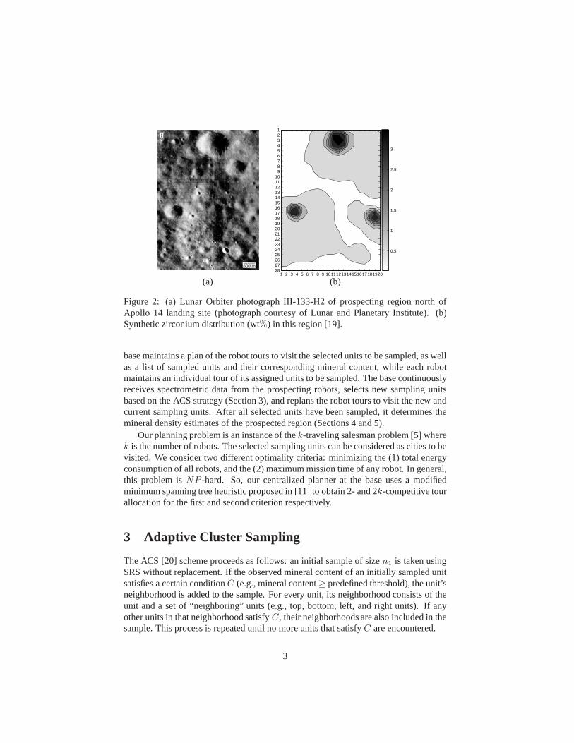
This paper presents adaptive sampling techniques for wide area prospecting witha team of robots (Fig. 1). Assume that the prospecting region(Fig. 2a) is discretizedinto a grid ofN sampling units.Adaptive samplingrefers to sampling strategies inwhich the procedure for selecting units to be included in thesample depends on themineral concentration observed during prospecting. In contrast, conventional samplinghas no such dependence. The main objective of adaptive sampling is to exploit the pop-ulation characteristics of mineral deposits (e.g., spatial clustering or patchiness shownin Fig. 2b) to obtain more precise estimates of the regional density than conventionalstrategies for a given sample size or cost.

This paper describes a specific adaptive sampling scheme known as ACS (Sec-tion 3), which has a number of desirable benefits for multi-robot wide area prospecting:(1) it returns a higher mineral yield and more information about the prospected regionby directing robot exploration towards areas of high mineral density, thus providingdetailed maps of the boundaries of such areas, and (2) it reduces the total mission time

1

Figure 1: Multi-robot mineral prospecting task.

and energy consumption of the robot team (Section 7).The adaptive nature of this scheme incurs a considerable bias in conventional es-

timators due to a large proportion of high mineral content data in the sample. Conse-quently, two unbiased estimators are proposed in [20] for the ACS strategy (Section 4).This paper investigates how the error of these estimators can be reduced through a pro-cess known asRao-Blackwellization, in which the outputs of the estimators are aver-aged over several different ordered samples that are constructed by permuting the orig-inal sampled data. The Rao-Blackwellization procedure is elaborated in Section 5; inthat section, its computational expense is also addressed,and closed-form expressionsare provided for the Rao-Blackwellized estimators. Since the efficiency of estimatorsdepends on the type of mineralogical population sampled, the population characteris-tics that favor ACS estimators are also analyzed (Section 6). Before discussing the ACSstrategy and estimators, an overview of the multi-robot architecture will be presentedfirst in the next section.

2 Robot Supervision Architecture

The mineral prospecting task demonstrates an application of the Robot SupervisionArchitecture (RSA) in our project called PROSPECT: Planetary Robots Organized forSafety and Prospecting Efficiency via Cooperative Telesupervision(http://www.ri.cmu.edu/∼prospect). This project is supported by NASA’s ExplorationSystems Mission Directorate. Our primary goal is to developa general architecture forhuman supervision of an autonomous robot team in support of sustained, affordable,and safe space exploration.

The RSA comprises the teleoperation base and robot prospectors. The teleoperation

2

1 2 3 4 5 6 7 8 9 1011121314151617181920

123456789

10111213141516171819202122232425262728

0.5

1

1.5

2

2.5

3

(a) (b)

Figure 2: (a) Lunar Orbiter photograph III-133-H2 of prospecting region north ofApollo 14 landing site (photograph courtesy of Lunar and Planetary Institute). (b)Synthetic zirconium distribution (wt%) in this region [19].

base maintains a plan of the robot tours to visit the selectedunits to be sampled, as wellas a list of sampled units and their corresponding mineral content, while each robotmaintains an individual tour of its assigned units to be sampled. The base continuouslyreceives spectrometric data from the prospecting robots, selects new sampling unitsbased on the ACS strategy (Section 3), and replans the robot tours to visit the new andcurrent sampling units. After all selected units have been sampled, it determines themineral density estimates of the prospected region (Sections 4 and 5).

Our planning problem is an instance of thek-traveling salesman problem [5] wherek is the number of robots. The selected sampling units can be considered as cities to bevisited. We consider two different optimality criteria: minimizing the (1) total energyconsumption of all robots, and the (2) maximum mission time of any robot. In general,this problem isNP -hard. So, our centralized planner at the base uses a modifiedminimum spanning tree heuristic proposed in [11] to obtain 2- and 2k-competitive tourallocation for the first and second criterion respectively.

3 Adaptive Cluster Sampling

The ACS [20] scheme proceeds as follows: an initial sample ofsizen1 is taken usingSRS without replacement. If the observed mineral content ofan initially sampled unitsatisfies a certain conditionC (e.g., mineral content≥ predefined threshold), the unit’sneighborhood is added to the sample. For every unit, its neighborhood consists of theunit and a set of “neighboring” units (e.g., top, bottom, left, and right units). If anyother units in that neighborhood satisfyC, their neighborhoods are also included in thesample. This process is repeated until no more units that satisfy C are encountered.

3

At this stage, clusters of units are obtained. Eachclustercontains units that satisfyC and a boundary ofedge units. An edge unitis a unit that does not satisfyC but isin the neighborhood of a unit that does. The final sample of sizeν consists of up ton1

clusters. These clusters are not necessarily distinct, since two units in the initial samplethat satisfyC could have been selected from the same cluster. If a unit in the initialsample does not satisfyC, it is considered to be a cluster of size one.

Let thenetworkAi that is generated by uniti be defined as a cluster generatedby that unit with its edge units removed. A selection of any unit in Ai leads to theselection of all units inAi. Any unit that does not satisfyC is a network of size onesince its selection does not lead to the inclusion of any other units. This implies thatany edge unit is also a network of size one. Hence, any clusterof size larger than 1 canbe decomposed into a network with units that satisfyC, and also networks (edge units)of size one that do not satisfyC. Clusters may overlap on their edge units. In contrast,networks are disjoint and form a partition of the entire population of units.

An example of an adaptive cluster sample is illustrated in Table 1. The valuesin this table are obtained in a simulation test run on the prospecting region in Fig. 2,which is discretized into a28×20 grid of square sampling units (thus, the total numberof units N = 560). The neighborhood of a unit is defined to be the top, bottom,left, and right units. The condition for sampling a unit’s neighborhood is defined asC = (y ≥ 1.0 wt%) wherey is the observed mineral content of a sampling unit. Withan initial sample sizen1 of 80, the ACS scheme results in a final sample sizeν of150. The boxed values correspond to units from the initial sample. The lightly anddarkly shaded units correspond to network and edge units respectively. 3 networks ofsize larger than 1 can be observed in the sample (Table 1). Notice that the leftmostnetwork is intersected 4 times by the initial sample while the other two networks areeach intersected once.

A noteworthy aspect of ACS is that given a fixedν, the travel cost of adding acluster or network of “neighboring” units in ACS is usually lower than that of addingunits selected at random using SRS in the prospecting region. This is demonstratedempirically in Section 7.

Since the ACS scheme results in a large proportion of high mineral content datain the sample, it will incur a considerable bias with the conventional sample meanestimatorµ = ν−1

∑ν

i=1yi. Kriging (or Gaussian process regression) [4] is a more

sophisticated alternative but will be similarly biased. For example, the true populationmeanµ is 0.648 for the zirconium distribution in Fig. 2b. However,for the ACS exam-ple in Table 1,µ = 1.070 with var[µ] = 0.004139 (i.e., standard error of 0.064), whichclearly overestimatesµ. Hence, unbiased estimators are needed for the ACS scheme.Two of these are presented in the next section.

4 Unbiased ACS Estimators

4.1 Modified Horvitz-Thompson Estimator

The first ACS estimator is modified from the Horvitz-Thompson(HT) estimator [8].LetBi be the set of units in theith network andmi be the number of units inBi. Note

4

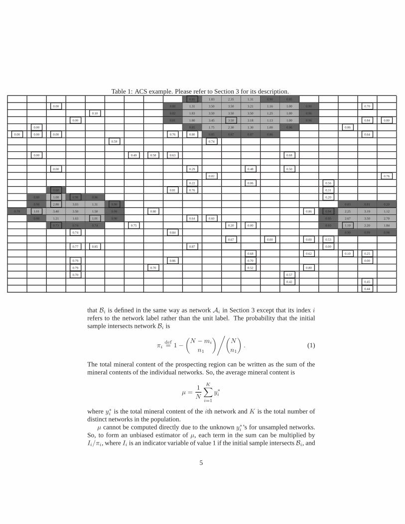
Table 1: ACS example. Please refer to Section 3 for its description.0.85 1.83 2.35 1.31 0.90 0.85

0.00 0.80 1.31 3.50 3.50 3.21 1.16 1.00 0.90 0.70

0.10 0.82 1.83 3.50 3.50 3.50 1.25 1.00 0.96

0.00 0.81 1.80 3.45 3.50 3.18 1.13 1.00 0.96 0.84 0.80

0.00 0.85 1.75 2.30 1.30 1.00 0.96 0.86

0.00 0.00 0.00 0.76 0.80 0.85 0.87 0.87 0.86 0.64

0.59 0.74

0.00 0.49 0.58 0.63 0.68

0.00 0.29 0.48 0.50

0.02 0.76

0.22 0.06 0.56

0.60 0.81 0.76 0.31

0.80 1.00 0.98 0.86 0.20

0.98 2.88 3.03 1.31 0.90 0.83 0.81 0.20

0.79 1.01 3.40 3.50 1.50 0.99 0.80 0.86 0.94 2.25 3.19 1.12

0.88 1.21 1.63 1.01 0.90 0.64 0.60 0.95 2.67 3.50 2.70

0.73 0.74 0.74 0.75 0.20 0.00 0.93 1.10 2.20 1.84

0.74 0.84 0.90 0.99 0.98

0.67 0.00 0.00 0.53

0.77 0.85 0.87 0.00

0.68 0.62 0.10 0.25

0.79 0.86 0.70 0.00

0.79 0.70 0.52 0.80

0.70 0.57

0.42 0.45

0.44

thatBi is defined in the same way as networkAi in Section 3 except that its indexirefers to the network label rather than the unit label. The probability that the initialsample intersects networkBi is

πidef= 1 −

(N − mi

n1

)/(N

n1

). (1)

The total mineral content of the prospecting region can be written as the sum of themineral contents of the individual networks. So, the average mineral content is

µ =1

N

K∑

i=1

y∗i

wherey∗i is the total mineral content of theith network andK is the total number of

distinct networks in the population.µ cannot be computed directly due to the unknowny∗

i ’s for unsampled networks.So, to form an unbiased estimator ofµ, each term in the sum can be multiplied byIi/πi, whereIi is an indicator variable of value 1 if the initial sample intersectsBi, and

5

0 otherwise. The expected value ofIi/πi is 1 for sampled networks, so our estimatoris unbiased; sinceIi is 0 for unsampled networks, information about these networksare not needed to calculate our estimator. Applying this trick yields themodified HTestimatorof µ:

µHT =

K∑

i=1

y∗i Ii

Nπi

=

κ∑

i=1

y∗i

Nπi

(2)

whereκ is the number of distinct networks intersected by the initial sample.For practical use of the HT estimator, it is important to be able to estimate its

variance from the sample. There is a simple closed-form formula which can be used forthis purpose.πi has been defined to be the probability that the initial sampleintersectstheith network. Defineπjk to be the probability that the initial sample intersects boththejth andkth networks. Ifj = k, thenπjk = πj . Otherwise, to computeπjk, noticethat the probability that the initial sample intersects neither networkj nor networkk is

P(Ij 6= 1 ∩ Ik 6= 1) =

(N − mj − mk

n1

)/(N

n1

).

So, the probability that the initial sample intersects either jth or kth network is1−P(Ij 6= 1 ∩ Ik 6= 1), and

πjk = πj + πk − (1 − P(Ij 6= 1 ∩ Ik 6= 1)) .

SinceµHT is a sum of several terms, its variance can be derived by taking the sumof covariances between these terms:

var[µHT ] =

K∑

j=1

K∑

k=1

cov[y∗

j Ij

Nπj

,y∗

kIk

Nπk

]

=

K∑

j=1

K∑

k=1

y∗j

Nπj

y∗k

Nπk

cov[Ij , Ik] .

(3)

(3) cannot be computed from the sample data since not all the networks in the popula-tion are necessarily sampled. So, to obtain an unbiased estimator of the variance, wecan use a similar trick as before: each term is multiplied byIjIk/πjk (which has anexpected value of 1 for sampled networks) to get

var[µHT ] =

K∑

j=1

K∑

k=1

y∗j Ij

Nπj

y∗kIk

Nπk

cov[Ij , Ik]

πjk

=1

N2

κ∑

j=1

κ∑

k=1

y∗j y∗

k

πjk

(πjk

πjπk

− 1

)

.

(4)

The second equality follows because cov[Ij, Ik] is πjk − πjπk.For the ACS example in Table 1,µHT = 0.665 andvar[µHT ] = 0.001835 (i.e.,

standard error of 0.043) by using (2) and (4) respectively.

6

4.2 Modified Hansen-Hurwitz Estimator

The second ACS estimator is modified from the Hansen-Hurwitz(HH) estimator [7].In the previous section, we mention that the total mineral content of the prospectingregion is the sum of the mineral contents of the individual networks. The mineralcontent of each network can be written as the average mineralcontent of all units inthis network summed over its number of network units. So, theaverage mineral contentof the prospecting region can also be expressed as

µ =1

N

N∑

i=1

wi

wherewi is the average mineral content of the networkAi containing uniti.µ cannot be computed directly due to the unknownwi’s for unsampled networks.

Using the same trick as in the previous section, an unbiased estimator ofµ can beformed by multiplying each term in the sum withNJi/n1, whereJi is an indicatorvariable of value 1 if uniti is included in the initial sample, and 0 otherwise. Theexpected value ofNJi/n1 is 1 for initial sample units, so our estimator is unbiased;sinceJi is 0 for units not in the initial sample, information about these units is notneeded to calculate our estimator. Applying this trick yields themodified HH estimatorof µ:

µHH =1

n1

N∑

i=1

wiJi =1

n1

n1∑

i=1

wi (5)

Note thatµHH can be interpreted as the conventional sample mean obtainedusing SRSof sizen1 from a population ofwi values rather thanyi values. So, using the theory ofSRS [20],

var[µHH ] =N − n1

Nn1(N − 1)

N∑

i=1

(wi − µ)2 (6)

with unbiased estimator

var[µHH ] =N − n1

Nn1(n1 − 1)

n1∑

i=1

(wi − µHH)2 . (7)

For the ACS example in Table 1,µHH = 0.624 andvar[µHH ] = 0.002802 (i.e.,standard error of 0.053) by using (5) and (7) respectively.

5 Improved Unbiased Rao-Blackwellized ACS Estima-tors

An estimatort(Do) of a population characteristicµ is a functiont which maps ourobserved dataDo to an estimate ofµ. Saying thatµ is a population characteristicmeans there is a parameter vectorθ which completely describes the distribution of ourpopulation, andµ = µ(θ) is a function of this parameter vector.

7

In our setting,Do is an ordered list of pairs〈is, yis〉 whereis is the unit sampled

at steps and yisis its mineral content. The population characteristic of interestµ

is the average mineral content of the sampling region. The population parameter isθ = 〈y1, . . . , yN 〉, which is the vector of true mineral contents for all units inthepopulation. The estimators ofµ that we are interested in areµHT andµHH .

To evaluate an estimatort(Do), its distribution conditioned on a possible value ofθcan be examined. Good estimators have low mean-squared errors, i.e., the distributionP(t(D0) − µ|θ) is concentrated around 0. In this section, we will describea way toreduce the mean-squared errors of the estimatorsµHT andµHH .

Rao-Blackwellization is a procedure that allows us to reduce the mean-squared er-ror of an arbitrary estimatort(Do). The improved estimator is E(t(Do)|D) whereD isa reduced description of our data that omits some redundant information. In particular,D is defined as astatisticif it is a function of our dataDo, andD is defined as asuffi-cient statisticif it contains all relevant information inDo aboutθ, i.e., P(Do|D, θ) =P(Do|D).

Given these definitions, Rao-Blackwellization is the process of computing E(t(Do)|D)whenD is a sufficient statistic. In our case,D is set to be theunorderedset of distinct,labeled observations, i.e.,D = {〈i, yi〉| i ∈ S} whereS is the set of distinct unit labelsin our data sample [20].

The following theorem, adapted from the Rao-Blackwell theorem [2], justifies theuse of the Rao-Blackwellized (RB) estimator:

Theorem 1 Let t = t(Do) be a (not necessarily unbiased) estimator ofµ. DefinetD = E[t|D]. Then(a) tD is an estimator;(b) E[tD] = E[t];(c) MSE[tD] ≤ MSE[t] with strict inequality for allθ such that Pθ(t 6= tD) > 0.

Corollary 1 If t is unbiased,

var[tD] = var[t] − EDE[(t − tD)2|D]= var[t] − ED{var[t|D]} .

(8)

The proofs of Theorem 1 and Corollary 1 are provided in Appendices A and B respec-tively. From (8), var[tD] ≤ var[t] since the variance reduction term ED{var[t|D]} ≥ 0.

Rao-Blackwellization does nothing ifg(Do) is already a function ofD. On theother hand, it achieves the largest possible reduction in variance whenD is aminimalsufficient statistic. A minimal sufficient statistic is one that reducesDo as much aspossible without losing information aboutθ:

Definition 1 A sufficient statisticD = g(Do) is minimal sufficientfor θ if, for anyother sufficient statisticD′ = g′(Do), D is a function ofD′.

In our case,D is minimal sufficient, andµHT and µHH are not functions ofD;they depend on the order of selection. To see this, consider asmall population of fourunits withθ = [0.1, 0.5, 1, 2]T . The condition isy ≥ 1. The initial sample sizen1 is2. The initial samples (〈2, 0.5〉, 〈3, 1〉) and (〈3, 1〉, 〈4, 2〉) give the same final unordered

8

sampleD = {〈2, 0.5〉, 〈3, 1〉, 〈4, 2〉}. Note that the edge unit〈2, 0.5〉 is included in thefirst initial sample but not the second one. This implies the edge unit will be involved incomputingµHT or µHH only in the first sample. Hence, either estimator will producedifferent estimates for the two samples.

In order to Rao-BlackwellizeµHT andµHH , we will need several notations. LetG =

(νn1

)be the number of combinations ofn1 distinct initial sample units from the

ν units in the final sample and let these combinations be indexed by the labelg whereg = 1, 2, . . . , G. Let τg be the value of an estimatort when the initial sample consistsof combinationg, Ig be an indicator variable of value 1 if thegth combination canresult inD (i.e., iscompatiblewith D), and 0 otherwise. The number of compatiblecombinations is thenξ =

∑G

g=1Ig. It follows that P(t = τg|D) = 1/ξ for all compatible

g. So, the improved RB estimator is

tRB = E[t|D] =1

ξ

G∑

g=1

τgIg =1

ξ

ξ∑

g=1

τg . (9)

The variance oftRB is obtained using (8) wheretD = tRB . The unbiased estimator ofvar[tRB] is then

var[tRB ] = var[t] − var[t|D] = var[t] −1

ξ

ξ∑

g=1

(τg − tRB)2 . (10)

Since (9) and (10) are based on samples compatible withD, naively, theξ compat-ible samples have to be identified from theG combinations and their correspondingξestimators have to be evaluated.ξ andG can be potentially large, which would ren-der the RB method computationally infeasible. However, in the next two subsections,closed-form expressions for the RBHT and RBHH estimators [16] will be described.

5.1 Rao-Blackwellized HT Estimator

The reason that the HT estimator yields different values with different compatible sam-ples is each compatible sample intersects a different combination of the edge units inthe final sampleD (in contrast, all networks other than the edge units must be includedin every compatible sample). So, some of the indicator variables in (2) will have dif-ferent values in different compatible samples.

The closed-form expression for the RBHT estimator is based on the observationthat we can analytically compute the expectation of each of the indicator variables in(2) given a randomly selected compatible sample. This expectation will be 1 for allnetworks of size greater than 1 and for all networks of size 1 that are not edge units.For networks that are edge units, the expectation will be strictly positive and less than1.

As we will see below, computing these expectations requiresevaluating several bi-nomial coefficients. The number of binomial coefficients is exponential in the numberof networks of size greater than 1. So, computing the RBHT estimator will be efficientif relatively few networks of size larger than 1 are intersected by the initial sample.

9

This assumption is reasonable because a prospecting regiontypically contains only afew major mineral deposits.

Since the modified HT estimator is formulated based on networks, its RB versionwill be derived likewise. LetE be the set of network labels in the sample. From (2),µHT for thegth combination can be written as

µgHT =

∑

i∈E

y∗i

Nπi

Igi (11)

whereIgi is an indicator variable of value 1 if thegth combination contains at least oneunit fromBi, and 0 otherwise.

By substituting (11) into (9), we get the RBHT estimator ofµ:

µRBHT =1

ξ

ξ∑

g=1

∑

i∈E

y∗i

Nπi

Igi =∑

i∈E

y∗i

Nπi

ξ∑

g=1

Igi

ξ(12)

where∑ξ

g=1Igi is the number of combinations containing at least one unit fromBi.

Clearly,ξ and∑ξ

g=1Igi in (12) have to be evaluated in order to obtain the closed-form

expression ofµRBHT . This can be achieved by evaluating them based on the differenttypes of network in the sample.

The sampleD can be partitioned into three different types of network: (a) networksof size larger than 1, (b) networks that are edge units, and (c) networks of size one thatare not edge units. More formally,E = F1∪F2∪F3 where (a)F1 = {i ∈ E| mi > 1},(b)F2 = {i ∈ E| Bi is an edge unit}, and (c)F3 = {i ∈ E − F1 −F2}.

ξ can be determined as follows: every network inF3 must be intersected by theinitial sample and is thus allocated one initial sample uniteach. The remainingn′

1 =n1 − |F3| initial sample units can be chosen fromν′ = ν − |F3| final sample units in(

ν′

n′

1

)ways. From these

(ν′

n′

1

)ways, combinations that are not compatible withD have

to be removed to getξ. These incompatible combinations are the ones that containnounits from at least one of the networks inF1. Formally, ifCi is the set of combinationscontaining no units fromBi, ∪i∈F1

Ci is the set of incompatible combinations that con-tain no units from at least one of the networks inF1. Using the inclusion-exclusionidentity for the cardinality of set union,

∣∣∣∣ ∪i∈F1

Ci

∣∣∣∣ =∑

i∈F1

|Ci| −∑

i,j∈F1

|Ci ∩ Cj | + . . . + (−1)|F1−1|

∣∣∣∣ ∩i∈F1

Ci

∣∣∣∣

=∑

i∈F1

(ν′ − mi

n′1

)−∑

i,j∈F1

(ν′ − mi − mj

n′1

)

+ . . . + (−1)|F1−1|

(ν′ −

∑i∈F1

mi

n′1

).

Then the number of compatible combinations is simply

ξ =

(ν′

n′1

)−

∣∣∣∣ ∪i∈F1

Ci

∣∣∣∣ . (13)

10

Since all compatible combinations contain at least one unitfrom each network inF1 ∪ F3,

∑ξ

g=1Igi = ξ for i ∈ F1 ∪ F3. This takes care of the cases (a) and (c).

However, each edge unit inF2 is not necessarily included in every combination. Toinclude an edge unit in a combination, one initial sample unit has to be allocated to theedge unit, which results inν′ − 1 units inD andn′

1 − 1 initial sample units. So, if welet ξ1 be the number of combinations containing the edge unitBi (i.e.,

∑ξ

g=1Igi = ξ1

for i ∈ F2), ξ1 is similar toξ except that both terms in every binomial coefficient arereduced by one. Substitutingξ andξ1 into (12),

µRBHT =∑

i∈F1∪F3

y∗i

Nπi

+ξ1

ξ

∑

i∈F2

y∗i

Nπi

. (14)

From (14),µRBHT is similar toµHT except that all edge units inF2 are now involvedbut each edge unit term is weighted byξ1/ξ. Hence,µRBHT is improved fromµHT

by using all information from the edge units. This is also therationale for improvingthe variance estimate ofµRBHT , which will be described next.

It is shown in Appendix C that

var[µHT |D] =1

(n1ξ)2

(ξ1ξ − ξ2

1)∑

i∈F2

y∗2i + 2(ξ2ξ − ξ2

1)∑

i∈F2

∑

j<i

y∗i y∗

j

(15)

whereξ2 is the number of combinations containing any two edge units in F2. Twoinitial sample units are allocated to two edge units, resulting in ν′ − 2 units inD andn′

1−2 initial sample units. So,ξ2 is similar toξ except that both terms in every binomialcoefficient are reduced by two. From (10), the unbiased estimator of var[µRBHT ] is

var[µRBHT ] = var[µHT ] − var[µHT |D] (16)

wherevar[µHT ] and var[µHT |D] are previously determined using (4) and (15) re-spectively. It can be observed from ( 15) that the variance reduction term var[µHT |D]depends solely on they-values of the edge units. Hence, the improvement in the RBHTestimator becomes smaller as they-values of the edge units tend to zero. For the ACSexample in Table 1,µRBHT = 0.656 andvar[µRBHT ] = 0.001574 (i.e., standard er-ror of 0.040) by using (14) and (16) respectively. The standard error is only reducedby 0.003, which is expected since they-values of the edge units are less than 1.0 (Sec-tion 3).

Note thatξ, ξ1, andξ2 each requires2|F1| binomial coefficients to be evaluated.Hence, the expressions forµRBHT andvar[µRBHT ] are computationally efficient if|F1| is small, i.e., relatively few networks of size larger than 1are intersected by theinitial sample.

5.2 Rao-Blackwellized HH Estimator

The derivation of the closed-form expression for the RBHH estimator follows the samenotion as before: we evaluate expectations of indicator variables by counting how often

11

individual units are present in a compatible sample. In the RBHT estimator, the indi-cator variables for networks inF1∪F3 are always 1, and we only need to calculate theexpectations for the networks inF2. The RBHH estimator, on the other hand, uses in-dicator variables of individual units. As before, all unitsin F3 will be present in everycompatible sample and so, their indicator variables will always be 1. But, the indicatorvariables for the units in networks inF1 ∪ F2 will be strictly between 0 and 1: bothedge units and units in networks of size greater than 1 are notnecessarily included inall of the compatible samples.

Since the modified HH estimator is formulated based on thew-value for each unit,its RB version will be derived likewise. The setS of unit labels in the sampleD can bepartitioned into three different types of units: (a) units in networks of size larger than 1,(b) edge units, and (c) non-edge units in networks of size one. So,S = H1 ∪H2 ∪H3

where (a)H1 = {i ∈ S| unit i ∈ Bj , j ∈ F1}, (b)H2 = {i ∈ S| unit i ∈ Bj , j ∈ F2},and (c)H3 = {i ∈ S| unit i ∈ Bj , j ∈ F3}. Note that|H2| = |F2| and|H3| = |F3|.

Let Jgi be an indicator variable of value 1 if thegth combination contains uniti,and 0 otherwise. From (5),µHH for thegth combination can be expressed as

µgHH =

1

n1

∑

i∈S

wiJgi =1

n1

(∑

i∈H1∪H2

wiJgi +∑

i∈H3

wi

)(17)

since all unit labels inH3 must be in everygth combination. By substituting (17) into(9), the RBHH estimator ofµ is

µRBHH =1

ξ

ξ∑

g=1

1

n1

(∑

i∈H1∪H2

wiJgi +∑

i∈H3

wi

)

=1

n1

(1

ξ

∑

i∈H1∪H2

wi

ξ∑

g=1

Jgi +∑

i∈H3

wi

) (18)

where∑ξ

g=1Jgi = ξi is the number of combinations containing uniti. ξ can be

determined using (13) in the previous section. To obtainξi, one initial sample unit isallocated to uniti and each unit inH3, resulting inν′ − 1 = ν − |H3| − 1 units inDandn′

1 − 1 = n1 − |H3| − 1 initial sample units.ξi is then(

ν′−1

n′

1−1

)ways reduced by

the number of combinations that contain no unit label from atleast one of the networksin F1. For i ∈ H1, ξi is similar toξ1 except that we ignore the binomial coefficientsinvolving j ∈ F1 where uniti ∈ Bj. Fori ∈ H2, ξi = ξ1. Substitutingξi into (18),

µRBHH =1

n1

(1

ξ

∑

i∈H1∪H2

wiξi +∑

i∈H3

wi

). (19)

From (19),µRBHH differs from µHH by involving all network units inH1 and edgeunits, but each term with these units is weighted byξi/ξ. Hence,µRBHH is improvedfrom µHH by using all information from the network units inH1 and edge units, whichis also the case for improving the variance estimate ofµRBHH . Similar to deriving

12

var[µHT |D] in Appendix C,

var[µHH |D] =1

(n1ξ)2

( ∑

i∈H1∪H2

(ξiξ − ξ2

i )w2

i

+2∑

i∈H1∪H2

∑

j<i

(ξijξ − ξiξj)wiwj

) (20)

whereξij is the number of combinations containing unitsi andj in H1 ∪H2, that is,

ξij =

(ν′−2

n′

1−2

)−∑

x 6=k,l

(ν′−mx−2

n′

1−2

)if unit i ∈ Bk ∧ unit j ∈ Bl,

+∑

x,y 6=k,l

(ν′−mx−my−2

n′

1−2

)k, l ∈ F1,

+ . . . + (−1)|F1|(ν′−

P

mx−2

n′

1−2

)(

ν′−2

n′

1−2

)−∑

x 6=k

(ν′−mx−2

n′

1−2

)if (unit i ∈ Bk, k ∈ F1

+∑

x,y 6=k

(ν′−mx−my−2

n′

1−2

)∧ j ∈ H2) ∨ (unitsi, j ∈ Bk,

+ . . . + (−1)|F1|(ν′−

P

mx−2

n′

1−2

)k ∈ F1),

ξ2 if i, j ∈ H2

(21)

wherex, y ∈ F1. From (10), the unbiased estimator of var[µRBHH ] is

var[µRBHH ] = var[µHH ] − var[µHH |D] (22)

wherevar[µHH ] and var[µHH |D] are previously determined using (7) and (20) respec-tively. By comparing (15) and (20), we can observe that var[µHH |D] > var[µHT |D].If the y-values of the edge units tend to zero, var[µHH |D] depends more on thew-values of the network units inH1. Thus, the improvement of the RBHH estimatoris always greater than that of the RBHT estimator. For the ACSexample in Table 1,µRBHH = 0.648 andvar[µRBHT ] = 0.000720 (i.e., standard error of 0.027) by us-ing (19) and (22) respectively. The standard error is reduced by 0.026, which is morethan the reduction of 0.003 for the RBHT estimator (Section 5.1). Similar to the com-plexity analysis of RBHT estimator, the expressions forµRBHH andvar[µRBHH ] arecomputationally efficient if|F1| is small.

6 Efficiency Analysis of ACS Estimators

The efficiency of ACS over SRS depends on the type of mineralogical population beingsampled. In particular,µHH is more efficient than the conventional sample meanµ forSRS if var[µHH ] < var[µ]. Using the theory of SRS [20],

var[µ] =N − ν

Nν(N − 1)

N∑

i=1

(yi − µ)2 (23)

The total sum of squared difference betweenyi andµ in (23) can be partitioned intowithin-network and between-network components:

N∑

i=1

(yi − µ)2 =N∑

i=1

(yi − wi)2 +

N∑

i=1

(wi − µ)2 (24)

13

Using (6), (23), and (24), var[µHH ] < var[µ] if and only if

(1 −

n1

ν

) N∑

i=1

(yi − µ)2 <(1 −

n1

N

) N∑

i=1

(yi − wi)2 (25)

It can be observed from (25) thatµHH is more efficient thanµ if (1) the within-networkvariance of the population (rightmost term) is sufficientlyhigh, (2) the final sample sizeν is not much larger than the initial sample sizen1 for µHH so that1 − n1/ν is small,and (3)n1 ≪ N so that1 − n1/N is large. However, conditions 2 and 3 can opposecondition 1 because a small difference between initial and final sample size, and asmall initial sample size usually mean small within-network variance. So, ACS withµHH works best with networks that are small enough to restrict the final sample sizebut large enough for the within-network variance to represent the population variancereasonably. This means even though drastically lowering the threshold for conditionCcan increase the within-network variance and improve condition 1, it also increases thefinal sample size tremendously and violates condition 2 easily.

Although it is straightforward to compare var[µHT ] (3) and var[µ], it cannot beeasily interpreted since var[µHT ] involves the intersection probabilities. However, em-pirical results in Section 7 show thatµHT is consistently more efficient thanµ.

7 Experiments and Discussion

This section presents quantitative evaluations of the ACS scheme and its estimators forwide area prospecting with a team of four robots; this is the number of robots that willbe fielded on NASA Ames Research Center’s Moonscape for our project’s real-worldtest and evaluation. The experiments were performed using Webots, a mobile robotsimulator (http://www.cyberbotics.com). 16 directed distance sensors with 0.3 m rangewere modelled around its body of0.32 m (L)×0.27 m (W)×0.2 m (H). Each robotcould sense its global position through GPS1, and communicate spectrometric and tourdata with the base. The robots used the potential fields method [9] for navigationbetween sampling units and obstacle avoidance. Each robot could move at a maximumspeed of 0.425 m/s and consumed about 28.2 J/m. It used the Alpha Particle X-RaySpectrometer (APXS) [15] (1.3 W) for sampling, which required about 2 hours toobtain a high-quality x-ray spectrum of the mineral content. So, sampling each unitwould use about 9.5 kJ. The 6.46 km×4.61 km prospecting region is discretized intoa28×20 grid of sampling units such that each unit’s width is about 231 m. The robotswere placed at a sampling unit in the center of the region and had to rendezvous at thissame unit after all selected units were sampled.

To compare the performance of the estimators, the RMSE criterion is used to mea-sure their quality:

RMSE[t] =

[1

R

R∑

i=1

(τi − µ)2

] 1

2

1Deployment of space exploration infrastructure would ultimately result in GPS or similar localizationcapability on the Moon and Mars. If this is absent, the current technique of a sun-seeking sensor combinedwith local inertial navigation can be used.

14

whereR = 20 is the number of test runs,τi is the mean mineral content estimateobtained in test runi.

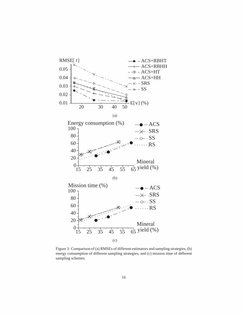
Using this measure, a quantitative test was conducted to compare the estimatorsdescribed above. For ACS, the initial sample sizen1 was 40, 80 or 240 samplingunits. After 20 test runs for eachn1, it resulted in an average final sample size E[ν]of approximately 95, 145, and 288 units, which correspondedto 17.1%, 25.7%, and51.4% of the 560 total sampling units. The SRS and SS schemes were conducted usingthe same sample sizes as E[ν].

Test results (Fig. 3a) show that the ACS estimators perform better than the non-ACSestimators. Among the ACS estimators, the Rao-Blackwellized estimators achievedlower RMSE. In particular, the differences in performance between the estimators werethe most significant at the sample size of 145 units. This implies that the ACS estima-tors, especially the Rao-Blackwellized ones, are practically more appealing becausemore accurate mineral density estimates can be obtained with a reasonably small sam-ple size. If the sample size decreases too much below 17.1%, the performance of allestimators will converge since their behavior will be more and more alike. If the samplesize increases too much beyond 51.4%, their performance will also converge due to in-creasing similarity in information from the prospecting region. Usingt-tests (α = 0.1),the differences in RMSEs between the estimators have been verified to be statisticallysignificant if these differences are more than 0.006 for the sample sizes of 95 and 145units, and more than 0.004 for the sample size of 288 units (see Appendix D). Note thatthe biased sample mean estimatorµ under the ACS scheme is not included in Fig. 3a;it has extremely large RMSEs of 0.525, 0.406, and 0.143 corresponding to 17.1%,25.7%, and 51.4% of the total sampling units.

To compare the system performance of the sampling schemes, the optimality cri-teria mentioned in Section 2 are considered: minimizing (1)total energy consumptionof all robots, and (2) maximum mission time of any robot. Fig.3b and c show the re-sults after 20 test runs for the first and second criterion respectively; the mineral yield,energy consumption, and mission time recorded for the various sampling strategies aregiven as a percentage of the corresponding values for RS (i.e., complete sampling of560 units). Note that each strategy (other than RS) has threedifferent records in itsplot, which correspond to E[ν] of 95, 145, and 288 units; a smaller sample size gives asmaller mineral yield. The line for RS shows a constant ratioof energy consumption ormission time to mineral yield. We observe that the ACS strategy yields more mineralsthan SRS and SS with less energy and mission time. The differences in mineral yield,energy consumption or mission time between ACS and the othertwo strategies havebeen verified usingt-tests (α = 0.1) to be statistically significant except for that ofenergy consumption between ACS and SS with a sample size of 145 units.

Furthermore, in contrast to SRS and SS, we observe that ACS falls below the dottedline of RS, which implies it achieves a lower ratio of energy consumption or missiontime to mineral yield than RS. Hence, it is both energy and time efficient to utilize ACSfor prospecting in place of RS. We also expect the advantage of ACS to increase whenthe sampling cost increases. For example, the alpha mode of APXS [15] requires atleast 8 hours of sampling time, while the Mossbauer spectrometer [10] runs at 2 W andneeds at least 6 hours. In our experiments for ACS, the spectrometry incurs 45% of thetotal energy consumption and 83% of the overall mission timefor a typical sample size

15

20 30 40 50 0.01

0.02

0.03

0.04

0.05 ACS+RBHH ACS+RBHT

ACS+HT ACS+HH

RMSE[ t ]

SRS

E[ ν ] (%)

SS

(a)

15 25 35 45 55 65 0

20

40

60

80

100 SRS ACS Energy consumption (%)

Mineral yield (%)

SS RS

(b)

15 25 35 45 55 65 0

20

40

60

80

100 SRS ACS Mission time (%)

Mineral yield (%)

SS RS

(c)

Figure 3: Comparison of (a) RMSEs of different estimators and sampling strategies, (b)energy consumption of different sampling strategies, and (c) mission time of differentsampling schemes.

16

of 288 units. These figures will increase substantially if the Mossbauer spectrometer isused instead.

8 Conclusion and Future Work

This paper describes the derivation of new low-error estimators within the ACS schemeand its application to multi-robot wide area prospecting. Quantitative experimental re-sults in the prospecting task simulation have shown that theACS scheme can yieldmore minerals with less resources and the Rao-Blackwellized ACS estimators can pro-vide more precise mineral density estimates than previous methods. For our futurework, we will apply these techniques on a larger robot team and real robots. Our plan-ner will be improved using other minimum spanning tree heuristics or stochastic searchstrategies to reduce the tour lengths so that ACS can be even more efficient than RS.We will also consider the effect of noisy and multivariate mineral content data on ourscheme and estimators. Lastly, adaptive systematic sampling will be examined.

References

[1] M. A. Batalin, M. Rahimi, Y. Yu, D. Liu, A. Kansal, G. S. Sukhatme, W. J. Kaiser,M. Hansen, G. J. Pottie, M. Srivastava, and D. Estrin. Call and response: Experimentsin sampling the environment. InProc. ACM SenSys’04, pages 25–38, 2004.

[2] D. Blackwell. Conditional expectation and unbiased sequential estimation.Ann. Math.Stat., 18(1):105–110, 1947.

[3] C. A. Carlson. Spatial distribution of ore deposits.Geology, 19(2):111–114, 1991.

[4] N. A. C. Cressie.Statistics for Spatial Data. Wiley, NY, 2nd edition, 1993.

[5] G. N. Frederickson, M. S. Hecht, and C. E. Kim. Approximation algorithms for somerouting problems.SIAM J. Comput., 7(2):178–193, 1978.

[6] B. Glass and G. Briggs. Evaluation of human vs. teleoperated robotic performance in fieldgeology tasks at a Mars analog site. InProc. 7th i-SAIRAS-03, 2003.

[7] M. M. Hansen and W. N. Hurwitz. On the theory of sampling from finite populations.Ann.Math. Stat., 14(4):333–362, 1943.

[8] D. G. Horvitz and D. J. Thompson. A generalization of sampling without replacement.J.Am. Stat. Assoc., 47(260):663–685, 1952.

[9] O. Khatib. Real-time obstacle avoidance for manipulators and mobile robots.Int. J. Robot.Res., 5(1):90–98, 1986.

[10] G. Klingelhofer, R. V. Morris, B. Bernhardt, D. Rodionov, P. A. de Souza Jr., S. W. Squyres,J. Foh1, E. Kankeleit, U. Bonnes, R. Gellert, C. Schroder, S. Linkin, E. Evlanov, B. Zubkov,and O. Prilutski. Athena MIMOS II Mossbauer spectrometer investigation.J. Geophys.Res., 108(E12), 2003.

[11] M. G. Lagoudakis, E. Markakis, D. Kempe, P. Keskinocak,A. Kleywegt, S. Koenig,C. Tovey, A. Meyerson, and S. Jain. Auction-based multi-robot routing. InProc. Robotics:Science and Systems, 2005.

17

[12] P. G. Lucey, D. T. Blewett, and B. L. Jolliff. Lunar iron and titanium abundance algo-rithms based on final processing of Clementine ultraviolet-visible images. J. Geophys.Res., 105(E8):20,297–20,305, 2000.

[13] P. G. Lucey, G. J. Taylor, and E. Malaret. Abundance and distribution of iron on the moon.Science, 268(5214):1150–1153, 1995.

[14] R. McCartney and H. Sun. Sampling and estimation by multiple robots. InProc. 4thICMAS-00, pages 415–416, 2000.

[15] R. Rieder, R. Gellert, J. Bruckner, G. Klingelhofer, G. Dreibus, A. Yen, and S. W. Squyres.The new Athena alpha particle X-ray spectrometer for the Mars exploration rovers.J.Geophys. Res., 108(E12):7,1–7,13, 2003.

[16] M. M. Salehi. Rao-Blackwell versions of the Horvitz-Thompson and Hansen-Hurwitz inadaptive cluster sampling.Environ. Ecol. Stat., 6(2):183–195, 1999.

[17] G. A. F. Seber and S. K. Thompson. Environmental adaptive sampling. In G. P. Patil andC. R. Rao, editors,Environmental Statistics, volume 12 ofHandbook of Statistics, pages201–220. North-Holland/Elsevier Sci. Publ., NY, 1994.

[18] P. D. Spudis and G. J. Taylor. The roles of humans and robots as field geologists on themoon. In W. W. Mendell, editor,2nd Conference on Lunar Bases and Space Activities ofthe 21st Century, NASA Conf. Pub. 3166, pages 307–313. 1992.

[19] G. J. Taylor and L. M. V. Martel. Lunar prospecting.Adv. Space Res., 31(11):2403–2412,2003.

[20] S. K. Thompson.Sampling. John Wiley & Sons, Inc., NY, 2002.

A Proof of Theorem 1

(a) SinceD is minimally sufficient forθ, E[t|D] does not depend onθ. HencetD doesnot depend onθ and can be regarded as an estimator;(b) E[tD] = EDE[t|D] = E[t];

(c) MSE[t] = E[(t − µ)2] = E[(t − tD + tD − µ)2]= E[(t − tD)2] + MSE[tD]

(26)

since

E[(t − tD)(tD − µ)] = EDE[(t − tD)(tD − µ)|D]= ED(tD − µ)E[(t − tD)|D]= ED(tD − µ)(E[t|D] − tD)= 0 .

(27)

It follows from (26) that MSE[tD] ≤ MSE[t] with equality if and only if E[(t−tD)2] =0 (i.e., t = tD with probability 1). Strict inequality will occur ift is different fromtDover a set of nonzero probability.

18

B Proof of Corollary 1

Given thatt is unbiased, E[t] = µ. Then

MSE[t] = E[(t − µ)2]= E[(t − E[t] + E[t] − µ)2]= var[t] + (E[t] − µ)2

= var[t] .

(28)

SincetD is also unbiased (Theorem 1), E[tD] = µ. Corollary 1 follows from (26) byusing (28) to replace MSE[t] and MSE[tD] with var[t] and var[tD] respectively.

C Derivation: var[ µHT | D]

µHT (2) for thegth combination can be expressed as

µgHT =

∑

i∈E

y∗i

Nπi

Igi =∑

i∈F1∪F3

y∗i

Nπi

+∑

i∈F2

y∗i

n1

Igi (29)

sinceπi = n1/N for networks of size one. Note thatI2gi = Igi,

∑ξ

g=1Igi = ξ1 for

i ∈ F2, IgiIgj = 1 if the gth combination contains at least one unit each fromBi

andBj, andIgiIgj = 0 otherwise. Since networksi andj in F2 are each of size 1,∑ξ

g=1IgiIgj = ξ2, i.e., the number of combinations containing any two edge units in

F2. By substituting (14) and (29) into the second term of (10),

var[µHT |D] =1

ξ

∑

g

(µgHT − µRBHT )2

=1

ξ

ξ∑

g=1

(∑

i∈F2

y∗i

n1

Igi −ξ1

ξ

∑

i∈F2

y∗i

n1

)2

=1

n21ξ3

ξ∑

g=1

(∑

i∈F2

y∗i (ξIgi − ξ1)

)2

=1

n21ξ3

ξ∑

g=1

∑

i∈F2

y∗2i (ξIgi − ξ1)

2

+2

n21ξ3

ξ∑

g=1

∑

i∈F2

∑

j<i

y∗i y∗

j (ξIgi − ξ1)(ξIgj − ξ1)

=1

n21ξ3

∑

i∈F2

y∗2i

ξ∑

g=1

(ξIgi − ξ1)2

+2

n21ξ3

∑

i∈F2

∑

j<i

y∗i y∗

j

ξ∑

g=1

(ξIgi − ξ1)(ξIgj − ξ1)

19

=1

n21ξ3

∑

i∈F2

y∗2i

ξ∑

g=1

(ξ2

1 + ξ2I2

gi − 2ξξ1Igi)

+2

n21ξ3

∑

i∈F2

∑

j<i

y∗i y∗

j

ξ∑

g=1

(ξ2IgiIgj − ξξ1Igi − ξξ1Igj + ξ2

1)

=1

n21ξ3

∑

i∈F2

y∗2i

(ξ∑

g=1

ξ2

1 + ξ2

ξ∑

g=1

Igi − 2ξξ1

ξ∑

g=1

Igi

)

+2

n21ξ3

∑

i∈F2

∑

j<i

y∗i y∗

j

(ξ2

ξ∑

g=1

IgiIgj

−ξξ1

ξ∑

g=1

Igi − ξξ1

ξ∑

g=1

Igj +

ξ∑

g=1

ξ2

1

)

=1

(n1ξ)2

∑

i∈F2

y∗2i (ξ1ξ − ξ2

1)

+2

(n1ξ)2

∑

i∈F2

∑

j<i

y∗i y∗

j (ξ2ξ − ξ1)2

=1

(n1ξ)2

((ξ1ξ − ξ2

1)∑

i∈F2

y∗2i

+2(ξ2ξ − ξ1)2∑

i∈F2

∑

j<i

y∗i y∗

j

).

20

D Significance levels fromt-tests on similarity inRMSEs between estimators

E[ν] = 95 SS SRS ACS+HH ACS+HT ACS+RBHHACS+RBHT 0.01 0.00 0.07 0.05 0.16ACS+RBHH 0.05 0.00 0.25 0.24

ACS+HT 0.16 0.00 0.48ACS+HH 0.20 0.00

SRS 0.01

E[ν] = 145 SS SRS ACS+HH ACS+HT ACS+RBHHACS+RBHT 0.00 0.00 0.02 0.02 0.01ACS+RBHH 0.00 0.01 0.17 0.16

ACS+HT 0.10 0.04 0.46ACS+HH 0.07 0.03

SRS 0.10

E[ν] = 288 SS SRS ACS+HH ACS+HT ACS+RBHHACS+RBHT 0.00 0.00 0.10 0.48 0.25ACS+RBHH 0.01 0.00 0.20 0.25

ACS+HT 0.00 0.01 0.10ACS+HH 0.16 0.01

SRS 0.02

21