adaptive sample-efficient blackbox optimization via es ... · ducting optimization of...
TRANSCRIPT
From Complexity to Simplicity: Adaptive ES-ActiveSubspaces for Blackbox Optimization
Krzysztof Choromanski*Google Brain [email protected]
Aldo Pacchiano*
Jack Parker-Holder*
Columbia [email protected]
Yunhao Tang*
Columbia [email protected]
Abstract
We present a new algorithm (ASEBO) for optimizing high-dimensional blackboxfunctions. ASEBO adapts to the geometry of the function and learns optimalsets of sensing directions, which are used to probe it, on-the-fly. It addresses theexploration-exploitation trade-off of blackbox optimization with expensive black-box queries by continuously learning the bias of the lower-dimensional model usedto approximate gradients of smoothings of the function via compressed sensing andcontextual bandits methods. To obtain this model, it leverages techniques from theemerging theory of active subspaces [8] in the novel ES blackbox optimization con-text. As a result, ASEBO learns the dynamically changing intrinsic dimensionalityof the gradient space and adapts to the hardness of different stages of the optimiza-tion without external supervision. Consequently, it leads to more sample-efficientblackbox optimization than state-of-the-art algorithms. We provide theoreticalresults and test ASEBO advantages over other methods empirically by evaluatingit on the set of reinforcement learning policy optimization tasks as well as functionsfrom the recently open-sourced Nevergrad library.
1 Introduction
Consider a high-dimensional function F : Rd → R. We assume that querying it is expensive.Examples include reinforcement learning (RL) blackbox functions taking as inputs vectors θ encodingpolicies π : S → A mapping states to actions and outputting total (expected/discounted) rewardsobtained by agents applying π in given environments [6]. For this class of functions evaluationsusually require running a simulator. Other examples include wind configuration design optimizationproblems for high speed civil transport aircrafts, optimizing computer codes (e.g. NASA synthetictool FLOPS/ENGENN used to size the aircraft and propulsion system [2]), crash tests, medical andchemical reaction experiments [37].
Evolution strategy (ES) methods have traditionally been used in low-dimensional regimes (e.g.hyperparameter tuning), and considered ill-equipped for higher dimensional problems due to poorsampling complexity [27]. However, a flurry of recent work has shown they can scale better thanpreviously believed [33, 11, 29, 25, 7, 30, 21]. This is thanks to a couple of reasons.
First of all, new ES methods apply several efficient heuristics (filtering, various normalizationtechniques as in [25] and new exploration strategies as in [11]) in order to substantially improvesampling complexity. Other recent methods [29, 7] are based on more accurate Quasi Monte Carlo(MC) estimators of the gradients of Gaussian smoothings of blackbox functions with theoretical
Preprint. Work in progress.
arX
iv:1
903.
0426
8v3
[m
ath.
OC
] 4
Jun
201
9

guarantees. These approaches provide better quality gradient sensing mechanisms. Additionally,in applications such as RL, new compact structured policy architectures (such as low-displacementrank neural networks from [7] or even linear policies [14]) are used to reduce the number of policies’parameters and dimensionality of the optimization problem.
Recent research also shows that ES-type blackbox optimization in RL leads to more stable policiesthan policy gradient methods since ES methods search for parameters that are robust to perturbations[19]. Unlike policy gradient methods, ES aims to find parameters maximizing expected reward (ratherthan just a reward) in respect to Gaussian perturbations.
Finally, pure ES methods as opposed to state-of-the-art policy optimization techniques (TRPO, PPOor ARS [32, 15, 31, 25]), can be applied also for blackbox optimization problems that do not exhibitMDP structure required for policy gradient methods and cannot benefit from state normalizationalgorithm central to ARS. This has led to their recent popularity for non-differentiable tasks [17, 14].
In this paper we introduce a new adaptive sample-efficient blackbox optimization algorithm. ASEBOadapts to the geometry of blackbox functions and learns optimal sets of sensing directions, whichare used to probe them, on-the-fly. To do this, it leverages techniques from the emerging theory ofactive subspaces [8, 10, 9, 20] in a novel ES blackbox optimization context. Active subspaces andtheir extensions are becoming popular as effective techniques for dimensionality reduction (see forinstance: active manifolds [5] or ResNets for learning isosurfaces [36]). However, to the best of ourknowledge we are the first to apply active subspace ideas for ES optimization.
ASEBO addresses the exploration-exploitation trade-off of blackbox optimization with expensivefunction queries by continuously learning the bias of the lower-dimensional model used to approx-imate gradients of smoothings of the function with compressed sensing and contextual banditsmethods. The adaptiveness is what distinguishes it from some recently introduced guided ES methodssuch as [24] that rely on fixed hyperparameters that are hard to tune in advance (e.g. the length ofthe buffer defining lower dimensional space for gradient search). We provide theoretical results andempirically evaluate ASEBO on a set of RL blackbox optimization tasks as well as non-RL blackboxfunctions from the recently open-sourced Nevergrad library [34], showing that it consistently learnsoptimal inputs with fewer queries to a blackbox function than other methods.
ASEBO versus CMA-ES: There have been a variety of works seeking to reduce sampling complexityfor ES methods through the use of metric learning. The prominent class of the covariance matrixadaptation evolution strategy (CMA-ES) methods derives state-of-the-art derivative free blackboxoptimization algorithms, which seek to learn and maintain a fully parameterized Gaussian distribution.CMA-ES suffers from quadratic time complexity for each evaluation which can be limiting for highdimensional problems. As such, a series of attempts have been made to produce scalable variantsof CMA-ES, by restricting the covariance matrix to the diagonal (sep-CMA-ES [28]) or a low rankapproximation as in VD-CMA-ES [3] and LM-CMA-ES [22]. Two recent algorithms, VkD-CMA-ES[4] and LM-MA-ES [23], seek to combine the above ideas and have been shown to be successful inlarge-scale settings, including RL policy learning [26]. Although these methods are able to quicklylearn and adapt the covariance matrix, they are heavily dependent on hyperparameter selection [4, 35]and lack the means to avoid learning a bias. As our experiments show, this can severely hurt theirperformance. The best CMA-ES variants often struggle with RL tasks of challenging objecivelandscapes, displaying inconsistent performance across tasks. Furthermore, they require carefulhyperparameter tuning for good performance (see: analysis in Section 4, Fig. 3).
2 Adaptive Sample-Efficient Blackbox Optimization
Before we describe ASEBO, we explain key theoretical ideas behind the algorithm. ASEBO usesonline PCA to maintain and update on-the-fly subspaces which we call ES-active subspaces LES
active,accurately approximating the gradient data space at a given phase of the algorithm. The bias of theobtained gradient estimators is measured by sensing the length of its component from the orthogonalcomplement LES,⊥
active via compressed sensing or computing optimal probabilities for exploration (e.g.sensing from LES,⊥
active) via contextual bandits methods [1]. The algorithm corrects its probabilisticdistributions used for choosing directions for gradient sensing based on these measurements. Aswe show, we can measure that bias accurately using only a constant number of additional functionqueries, regardless of the dimensionality. This in turn determines an exploration strategy, as weexplain later. Estimated gradients are then used to update parameters.
2

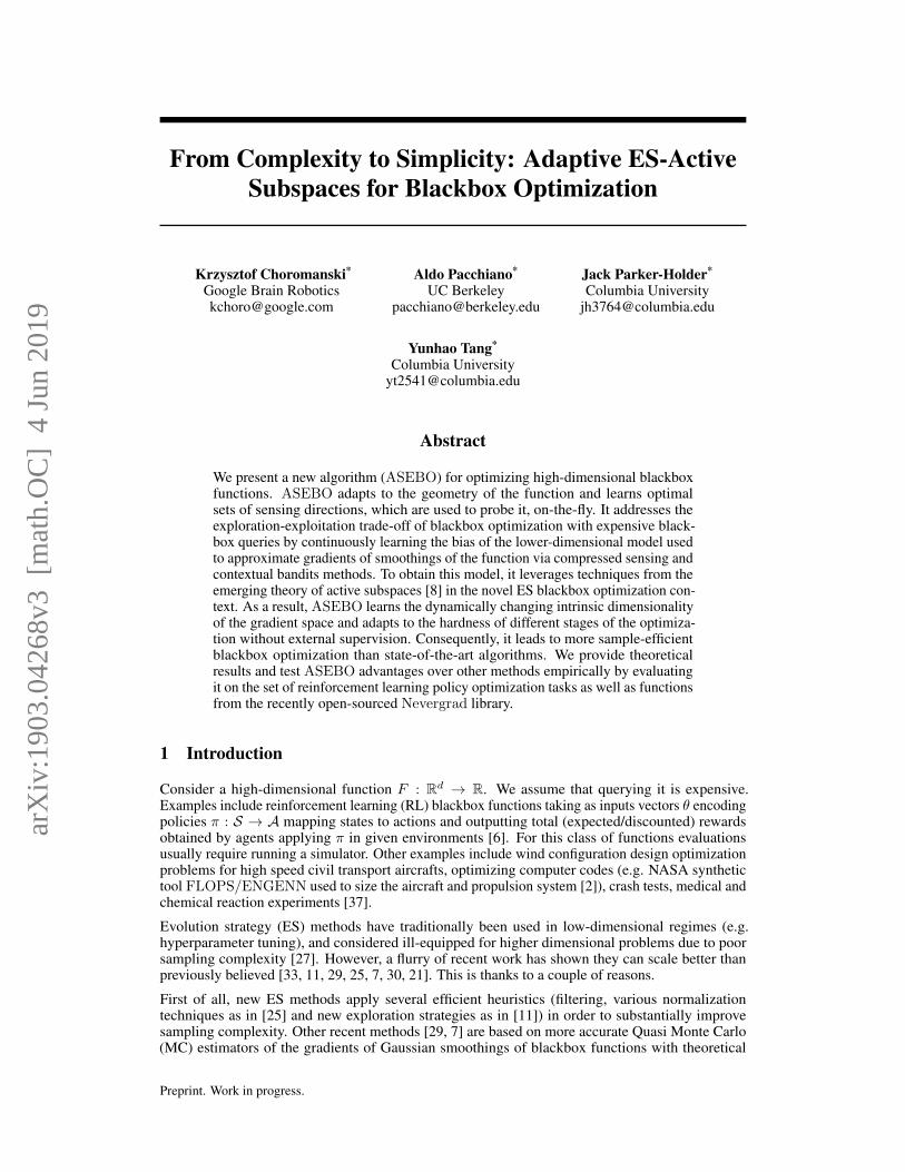
(a) HC: active subspace (b) SW: active subspace (c) HC: # of samples (d) SW: # of samples
Figure 1: The motivation behind ASEBO. Two first plots: ES baseline for HalfCheetah andSwimmer tasks from the OpenAI Gym library for 212-dimensional policies - the plot shows howthe dimensionality of the space capturing a given percentage of variance of approximate gradient datadepends on the iteration of the algorithm. This information is never exploited by the algorithm, eventhough 99.5% of the variance resides in the much lower-dimensional space (100 dimensions). Twolast plots: ASEBO taking advantage of this information (# of sample/sensing directions reflects thehardness of the optimization at each iteration and is strongly correlated with the PCA dimensionality.
2.1 Preliminaries
Consider a blackbox function F : Rd → R. We do not assume that F is differentiable. TheGaussian smoothing [27] Fσ of F parameterized by smoothing parameter σ > 0 is given as:
Fσ(θ) = Eg∈N (0,Id)[F (θ+ σg)] = (2π)−d2
∫Rd F (θ+ σg)e−
‖g‖22 dg. The gradient of the Gaussian
smoothing of F is given by the formula:
∇Fσ(θ) =1
σEg∼N (0,Id)[F (θ + σg)g]. (1)
Formula 1 on ∇Fσ(θ) leads straightforwardly to several unbiased Monte Carlo (MC) estimatorsof ∇Fσ(θ), where the most popular ones are: the forward finite difference estimator [7] definedas: ∇FD
MCFσ(θ) = 1kσ
∑ki=1(F (θ + σgi) − F (θ))gi, and an antithetic ES gradient estimator [30]
given as: ∇ATMCFσ(θ) = 1
2kσ
∑ki=1(F (θ + σgi) − F (θ − σgi))gi, where typically g1, ...,gk are
taken independently at random from N (0, Id) of from more complex joint distributions for variancereduction (see: [7]). We call samples g1, ...,gk the sensing directions since they are used to sensegradients∇Fσ(θ). The antithetic formula can be alternatively rationalized as giving the renormalizedgradient of F (if F is smooth), if not taking into account cubic and higher-order terms of the Taylorexpansion F (θ+v) = F (θ) +∇F>v+ 1
2v>H(θ)v (where H(θ) stands for the Hessian of F in θ).
Standard ES methods apply different gradient-based techniques such as SGD or Adam, fed withthe above MC estimators of∇Fσ to conduct blackbox optimization. The number of samples k periteration of the optimization procedure is usually of the order O(d). This becomes a computationalbottleneck for high-dimensional blackbox functions F (for instance, even for relatively small RLtasks with policies encoded by compact neural networks we still have d > 100 parameters).
2.2 ES-active subspaces via online PCA with decaying weights
The first idea leading to the ASEBO algorithm is that in practice one does not need to estimate thegradient of F accurately (after all ES-type methods do not even aim to compute the gradient of F , butrather focus on∇Fσ). Poor scalability of ES-type blackbox optimization algorithms is caused by high-dimensionality of the gradient vector. However, during the optimization process the space spannedby gradients may be locally well approximated by a lower-dimensional subspace L and sensingthe gradient in that subspace might be more effective. In some recent papers such as [24] such asubspace is defined simply as L = span{∇AT
MCFσ(θi), ∇ATMCFσ(θi−1), ..., ∇AT
MCFσ(θi−s+1)}, where{∇AT
MCFσ(θi), ∇ATMCFσ(θi−1), ..., ∇AT
MCFσ(θi−s+1)} stands for the batch of last s approximatedgradients during the optimization process and s is a fixed hyperparameter. Even though L willdynamically change during the optimization, such an approach has several disadvantages in practice.Tuning parameter s is very difficult or almost impossible and the assumption that the dimensionalityof L should be constant during optimization is usually false. In our approach, dimensionality of Lvaries and depends on the hardness of the optimization in different optimization stages.
We apply Principal Component Analysis (PCA, [18]) to create a subspace L capturing particularvariance σ > 0 of the approximate gradients data. This data is either: the approximate gradients
3

computed in previous iterations from the antithetic formula or: the elements of the sum from thatequation that are averaged over to obtain these gradients. For clarity of the exposition, from now onwe will assume the former, but both variants are valid. Choosing σ is in practice much easier than sand leads to subspaces L of varying dimensionalities throughout the optimization procedure, calledby us from now on ES-active subspaces LES
active.Algorithm 1 ASEBO AlgorithmHyperparameters: number of iterations of full sampling l, smoothing parameter σ > 0, step size η,PCA threshold ε, decay rate γ, total number of iterations T .Input: blackbox function F , vector θ0 ∈ Rd where optimization starts. Cov0 ∈ {0}d×d, p0 = 0.Output: vector θT .for t = 0, . . . , T − 1 do
if t < l thenTake nt = d. Sample g1, · · · ,gnt from N (0, Id) (independently).
else1. Take top r eigenvalues λi of Covt, where r is smallest such that:
∑ri=1 λi ≥ ε
∑di=1 λi,
using its SVD as described in text and take nt = r.2. Take the corresponding eigenvectors u1, ...,ur ∈ Rd and let U ∈ Rd×r be obtainedby stacking them together. Let Uact ∈ Rd×r be obtained from stacking together someorthonormal basis of LES
activedef= span{u1, ...,ur}. Let U⊥ ∈ Rd×(d−r) be obtained from
stacking together some orthonormal basis of the orthogonal complement LES,⊥active of LES
active.3. Sample nt vectors g1, ...,gnt as follows: with probability 1− pt from N (0,U⊥(U⊥)>)and with probability pt from N (0,Uact(Uact)>).4. Renormalize g1, ...,gnt such that marginal distributions ‖gi‖2 are χ(d).
1. Compute ∇ATMCF (θt) as: ∇AT
MCF (θt) = 12ntσ
∑ntj=1(F (θt + gj)− F (θt − gj))gj .
2. Set Covt+1 = λCovt + (1− λ)Γ, where Γ = ∇ATMCFσ(θt)(∇AT
MCFσ(θt))>.
3. Set pt+1 = popt for popt output by Algorithm 2 and: θt+1 ← θt + η∇ATMCF (θt).
These will be in turn applied to define covariance matrices encoding probabilistic distributions appliedto construct sensing directions used for estimating∇Fσ(θ). The additional advantage of our approachis that PCA automatically filters out gradient noise.
We use our own online version of PCA with decaying weights (decay rate is defined by parameterλ > 0). By tuning λ we can define the rate at which historical approximate gradient data is usedto choose the right sensing directions, which will continuously decay. We consider a stream ofapproximate gradients ∇AT
MCFσ(θ0), ...∇ATMCFσ(θi), ... obtained during the optimization procedure.
We maintain and update on-the-fly the covariance matrix Covt, where t stands for the number ofcompleted iterations, in the form of the symmetric matrix SVD-decomposition Covt = Q>t ΣtQt ∈Rd. When the new approximate gradient ∇AT
MCFσ(θt) arrives, the update of the covariance matrix isdriven by the following equation, reflecting data decay process, where xt = ∇AT
MCFσ(θt):Q>t+1Σt+1Qt+1 = λQ>t ΣtQt + (1− λ)xtx
>t , (2)
To conduct the update cheaply, it suffices to observe that the RHS of Equation 2 can be rewrittenas: λQ>t ΣtQt + (1 − λ)xtx
>t = Q>t (λΣt + (1 − λ)Qtxt(Qtxt)
>)Qt. Now, using the fact thatfor a matrix of the form D + uu>, we can get its decomposition in time O(d2) [13], we obtain analgorithm performing updates in quadratic time. That in practice suffices since the bottleneck of thecomputations is in querying F and additional overhead related to updating LES
active is negligible.
ES-active subspaces versus active subspaces: Our mechanism for constructing LESactive is inspired
by the recent theory of active subspaces [8], developed to determine the most important directions inthe space of input parameters of high-dimensional blackbox functions such as computer simulations.
The active subspace of a differentiable function F : Rd → R, square-integrable with respect to thegiven probabilistic density function ρ : Rd → R, is given as a linear subspace Lactive defined by thefirst r (for a fixed r < d) eigenvectors of the following d× d symmetric positive definite matrix:
Cov =
∫x∈Rd
∇F (x)∇F (x)>ρ(x)dx (3)
4

Density function ρ determines where compact representation of F is needed. In our approach we donot assume that∇F exists, but the key difference between LES
active and Lactive lies somewhere else.
The goal of ASEBO is to avoid approximating the exact gradient∇F (x) ∈ Rd which is what makesstandard ES methods very expensive and which is done in [9] via gradient sketching techniquescombined with finite difference approaches (standard methods of choice for ES baselines).
Algorithm 2 Explore estimator via exponentiated samplingHyperparameters: smoothing parameter σ, horizon C, learning rate α, probability regularizer β,initial probability parameter qt0 ∈ (0, 1).Input: subspaces: LES
active, LES,⊥active, function F , vector θt
Output:for l = 1, · · · , C + 1 do
1. Compute ptl−1 = (1− 2β)qtl−1 + β and sample atl ∼ Ber(ptl).3. If atl = 1, sample gl ∼ N (0, σILES
active), otherwise sample gl ∼ N (0, σILES,⊥
active).
4. Compute vl = 12σ (F (θt + gl)− F (θt − gl)).
5. Set el = (1− 2β)
(−a
tl(dim(LES
active)+2)(ptl)
3
)(− (1−atl)(dim(LES,⊥
active)+2)
(1−ptl)3
) v2l .
6. Set qtl =qtl−1 exp(−αel(1))
qtl−1 exp(−αel(1))+(1−qtl−1) exp(−αel(2)).
Return: pC .
Instead, in ASEBO an ES-active subspace LESactive is itself used to define sensing directions and
the number of chosen samples k is given by the dimensionality of LESactive. This drastically reduces
sampling complexity, but comes at a price of risking the optimization to be trapped in the fixedlower-dimensional space that will not be representative for gradient data as optimization progresses.We propose a solution requiring only a constant number of extra queries to F in the next sections.
2.3 Exploration-exploitation trade-off: Adaptive Exploration Mechanism
The procedure described above needs to be accompanied with an exploration strategy that willdetermine how frequently to choose sensing directions outside the constructed on-the-fly lower-dimensional ES-subspace LES
active. Our exploration strategies will be encoded by hybrid probabilisticdistributions for sampling sensing directions. The frequency of sensing from the distributions withcovariance matrices obtained from LES
active (corresponding to exploitation) and from its orthogonalcomplement LES,⊥
active or entire space (corresponding to exploration) will be given by weights encodingthe importance of exploitation versus exploration in any given iteration of the optimization. For avector x ∈ Rd denote by xactive its projection onto LES
active and by x⊥ its projection onto LES,⊥active.
The useful metric that can be used to update the above weights in an online manner in the tth iterationof the algorithm is the ratio: r = ‖(∇Fσ(θt))active‖2
‖(∇Fσ(θt))⊥‖2 . Smaller values of r indicate that current activesubspace is not representative enough for the gradient and more aggressive exploration needs to beconducted. In practice, we do not compute r explicitly, but rather its approximated version r.
One can simply take: r =‖(∇AT
MCFσ(θt−1))active‖2‖(∇AT
MCFσ(θt−1))⊥‖2, where ∇AT
MCFσ(θt−1) is obtained in the pre-
vious iteration. But we can do better. It suffices to separately estimate ‖(∇Fσ(θt))active‖2 and‖(∇Fσ(θt))⊥‖2. However we do not aim to estimate (∇Fσ(θt))active and (∇Fσ(θt))⊥. That wouldbe equivalent to computing exact estimate of∇Fσ(θt), defeating the purpose of ASEBO. Instead,we note that estimating the length of the unknown high-dimensional vector is much simpler thanestimating the vector itself and can be done in the probabilistic manner with arbitrary precision via theset of dot-product queries of size independent from dimensionality d via compressed sensing methods.We refine this approach and propose more accurate contextual bandits method that also relies ondot-product queries applied in the ES-context, but aims to directly approximate optimal probabilitiesof sampling from LES
active rather than approximating gradients components’ lengths (see Algorithm2 box, the compressed sensing baseline is presented in the Appendix). The related computationaloverhead is measured in constant number of extra function queries, negligible in practice.
5

2.4 The Algorithm
ASEBO is given in the Algorithm 1 box. The algorithm we apply to score relative importance ofsampling from the ES-active subspace LES
active versus from outside LESactive is in the Algorithm 2 box.
As we have already mentioned, it uses bandits method do determine optimal probability of samplingfrom LES
active. In the next section we show that by using these techniques we can substantially reducethe variance of ES blackbox gradient estimators if ES-active subspaces approximate the gradientdata well (which is the case for RL blackbox functions as presented in Fig. 1). Horizon lengths C inAlgorithm 2 which determines the number of extra function queries should be in practice chosen assmall constants. In each iteration of Algorithm 1 the number of function queries is proportional tothe dimensionality of the ES-active subspace LES
active rather than the original space.
3 Theoretical Results
We provide here theoretical guarantees for the ASEBO sampling mechanism (in Algorithm 1), wheresensing directions {gi} at time t are sampled from the hybrid distribution P : with probability ptfrom N (0, ILactive
) and with probability 1− pt from N (0, IL⊥active).
Following notation in Algorithm 1, let Uact ∈ Rd×r be obtained by stacking together vectors ofsome orthonormal basis of LES
active, where dim(LESactive) = r and let U⊥ ∈ Rd×(d−r) be obtained my
stacking together vectors of some orthonormal basis of its orthogonal complement LES,⊥active. Denote
by σ a smoothing parameter. We make the following regularity assumptions on F :
Assumption 1. F is L−Lipschitz, i.e. for all θ, θ′ ∈ Rd, |F (θ)− F (θ′)| ≤ L‖θ − θ′‖2.Assumption 2. F has a τ -smooth third order derivative tensor with respect to σ > 0, so thatF (θ + σg) = F (θ) + σ∇F (θ)>g + σ2
2 g>H(θ)g + 16σ
3F ′′′(θ)[v,v,v] for some v ∈ Rd(‖v‖2 ≤ ‖g‖2) satisfying |F ′′′(θ)[v,v,v] ≤ τ‖v‖32 ≤ τ‖g‖32.
Observe that: Eg∼P[gg>
]=
(ptUact (Uact)
>+ (1− pt)U⊥
(U⊥)>)
. Define C1 =(ptUact (Uact)
>+ (1− pt)U⊥
(U⊥)>)
. Let ∇AT,aseboMC,k=1 Fσ(θ) = C−1
1F (θ+σg)g+F (θ+σg)(−g)
2σ
be the gradient estimator corresponding to P . We will assume that σ is small enough, i.e.
σ < 135
√εmin(pt,1−pt)τd3 max(L,1) for some precision parameter ε > 0. Our first result shows that under
these assumptions, baseline and ASEBO estimators of ∇σF (θ) are also good estimators of∇F (θ):
Lemma 3.1. If F satisfies Assumptions 1 and 2, the estimators ∇AT,baseMC,k=1Fσ(θ) and ∇AT,asebo
MC,k=1 Fσ(θ)
are close to the true gradient ∇F (θ), i.e.:∥∥∥Eg∼N (0,Id)
[∇AT,base
MC,k=1Fσ(θ)]−∇F (θ)
∥∥∥ ≤ ε and∥∥∥Eg∼P
[∇AT,asebo
MC,k=1 Fσ(θ)]−∇F (θ)
∥∥∥ ≤ ε.3.1 Variance reduction via non isotropic sampling
We show now that under sampling strategy given by distribution P , the variance of the gradientestimator can be made smaller by choosing the probability parameter pt appropriately. Denote:dactive = dim(LES
active) and d⊥ = dim(LES,⊥active). Let Γ := dactive+2
pt sUact + d⊥+21−pt sU⊥ − ‖∇F (θ)‖2.
Theorem 3.2. The following holds for sUact = ‖(Uact)>∇F (θ)‖22 and sU⊥ = ‖(U⊥)>∇F (θ)‖22:
1. The variance of ∇AT,aseboMC,k=1 Fσ(θ) is close to Γ, i.e. |Var[∇AT,asebo
MC,k=1 Fσ(θ)]− Γ| ≤ ε.
2. The choice of pt that minimizes Γ satisfies pt∗ :=
√(sUact )(dactive+2)√
(sUact )(dactive+2)+√
(sU⊥ )(d
U⊥+2)and
the optimal variance Varopt corresponding to pt∗ satisfies: |Varopt − ∆| ≤ ε for ∆ =[√(sUact)(dactive + 2) +
√(sU⊥)(d⊥ + 2)
]2− ‖∇F (θ)‖2.
3. Varopt ≤ Var[∇AT,baseMC,k=1Fσ(θ)]+ε−|
√(sU⊥)(dactive + 2)−
√(sUact)(d⊥ + 2)|2 − 2‖∇F (θ)‖2︸ ︷︷ ︸λ
.
Furthermore, slack variable λ is always nonnegative.
6

Theorem implies that when sUact = (1 − α)‖∇F (θ)‖22 and sU⊥ = α‖∇F (θ)‖22, forsome α ∈ (0, 1), we have: Var[∇AT,base
MC,k=1Fσ(θ)] ≈ (d + 1)‖∇F (θ)‖2 whereas Varopt =
O ((1− α)(dactive + 1) + α(d⊥ + 1)). When dactive << d and α << 1: Varopt �Var[∇AT,base
MC,k=1Fσ(θ)].
3.2 Adaptive Mirror Descent
In Theorem 3.2 we showed that for appropriate choices of LESactive and pt, the gradient estimator
∇AT,aseboMC,k=1 Fσ(θ) will have significantly smaller variance than ∇AT,base
MC,k=1Fσ(θ). In this section weshow that Algorithm 2 provides an adaptive way to choose pt. Using tools from online learningtheory, we provide regret guarantees that quantify the rate at which this Algorithm 2 minimizes thevariance of ∇AT,asebo
MC,k=1 Fσ(θ) and converges to the optimal pt∗.
Let ptl =( ptl
1−ptl
). The main component Γ of the variance of ∇AT,asebo
MC,k=1 Fσ(θ) as a function of ptlequals Γ = `(ptl) = dactive+2
ptl(1)sUact + d⊥+2
ptl(2)sU⊥ − ‖∇F (θ)‖2 (Theorem 3.2). We have:
Theorem 3.3. Let ∆2 be the a 2-d simplex. Under assumptions: 1 and 2, if σ < 135
√εmin(pt,1−pt)τd3 max(L,1) ,
α = 2β2√C[(dactive+2)2s2
Uact+(d⊥+2)s2U⊥
]and ε = β3
2C(d+1) , Algorithm 2 satisfies:
1
CE
[C∑l=1
`(ptl)
]− min
p∈β+(1−2β)∆2
`(p) ≤ Varopt
β2√C
+1
C
4 Experiments
In our experiments we use different classes of high-dimensional blackbox functions: RL blackboxfunctions (where the input is a high-dimensional vector encoding a neural network policy π : S → Amapping states s to actions a and the output is the cumulative reward obtained by an agent applyingthis policy in a particular environment) and functions from the recently open-sourced Nevergradlibrary [34]. In practice one can setup the hyperparameters used by Algorithm 2 as follows: σ =0.01, C = 10, α = 0.01, β = 0.1, qt0 = 0.1. For each algorithm we used k = 5 seeds and obtainedcurves are median-curves with inter-quartile ranges presented as shadowed regions.
Figure 2: Comparison of different blackbox optimization algorithms on OpenAI Gym tasks. Allcurves are median-curves obtained from k = 5 seeds and with inter-quartile ranges presented asshadowed regions. For Reacher we present only 3 curves since LM-MA-ES and TRPO did not learn.
4.1 RL blackbox functions
We used the following environments from the OpenAI Gym library: Swimmer-v2, HalfCheetah-v2, Walker2d-v2, Reacher-v2, Pusher-v2 and Thrower-v2. In all experiments we used policiesencoded by neural network architectures of two hidden layers and with tanh nonlinearities, with> 100 parameters. For gradient-based optimization we use Adam. For this class of blackboxfunctions we compared ASEBO with other generic blackbox methods as well as those specializingin optimizing RL blackbox functions F , namely: (1) CMA-ES variants; we compare against tworecently introduced algorithms designed for high-dimensional settings (we use the implementation
7

of VkD-CMA-ES in the pycma open-source implementation from https : //github.com/CMA-ES/pycma), and that of LM-MA-ES from [26]), (2) Augmented Random Search (ARS) [25](we use implementation released by the authors at http : //github.com/modestyachts/ARS), (3)Proximal Policy Optimization (PPO) [32] and Trust Region Policy Optimization (TRPO) [31] (weuse OpenAI baseline implementation [12]). The results for four environments are on Fig. 2.
Table 1: Median rewards obtained across k = 5 seeds for seven RL environments. For eachenvironment the top two performing algorithms are bolded, while the bottom two are shown in red.
Median reward after # timestepsEnvironment Timesteps ASEBO ES ARS VkD-CMA LM-MA TRPO PPO
HalfCheetah 5.107 3821 1530 2420 -144 1632 -512 1514Swimmer 107 358 36 348 367 297 110 52Walker2d 5.107 9941 347 1112 1 18065 3011 2377Hopper 107 99949 626 1091 42 100199 1663 1310Reacher 105 −11 −10 -12 -1391 -173 -112 -196Pusher 105 −46 -48 −45 -1001 -467 -120 -316Thrower 105 −89 -96 -90 -796 -737 −85 -175
Sampling complexity is measured in the number of timesteps (environment transitions) used by thealgorithms. ASEBO is the only algorithm that performs consistently across all seven environments(see: Table 1), outperforming CMA-ES variants on all tasks aside from VkD-CMA-ES on Swimmerand LM-MA-ES on Walker2d. For environments such as Reacher, Thrower and Pusher, thesemethods perform poorly, drastically underperforming even Vanilla ES. On Fig. 3, we demonstratethe common problem of state-of-the-art CMA-ES methods: if the number of samples n is not carefullytuned, the algorithm does not learn. ASEBO does not have this problem since n is learned on-the-fly.
Figure 3: Sensitivity analysis for CMA-ES variants on the HalfCheetah (HC) and Walker2d (WA)tasks. In each setting, we run k = 5 seeds, solely changing the number of samples per iteration (orpopulation size) n.
4.2 Nevergrad blackbox functions
We tested functions: sphere, rastrigin, rosenbrock and lunacek (from the class of Bi-Rastrigin/Lunacek’s No.02 functions). All tested functions are 1000-dimensional. The resultsare presented on Fig. 4. ASEBO is the most reliable method across different functions.
Figure 4: Comparison of median-curves obtained from k = 5 seeds for different algorithms onNevergrad functions [34]. Inter-quartile ranges are presented as shadowed regions.
8

5 Conclusion
We proposed a new algorithm for optimizing high-dimensional blackbox functions. ASEBO adjustson-the-fly the strategy of choosing gradient sensing directions to the hardness of the problem at thecurrent stage of optimization and can be applied for both RL and non-RL problems. We providedtheoretical guarantees for our method and exhaustive empirical validation.
References[1] S. Agrawal, N. R. Devanur, and L. Li. Contextual bandits with global constraints and objective.
CoRR, abs/1506.03374, 2015.
[2] S. Ahmad and K. B. Thomas. Flight optimization system ( flops ) hybrid electric aircraft designcapability. 2013.
[3] Y. Akimoto, A. Auger, and N. Hansen. Comparison-based natural gradient optimization in highdimension. GECCO, 2014.
[4] Y. Akimoto and N. Hansen. Projection-Based Restricted Covariance Matrix Adaptation forHigh Dimension. GECCO, 2016.
[5] R. A. Bridges, A. D. Gruber, C. Felder, M. E. Verma, and C. Hoff. Active manifolds: Anon-linear analogue to active subspaces. CoRR, abs/1904.13386, 2019.
[6] G. Brockman, V. Cheung, L. Pettersson, J. Schneider, J. Schulman, J. Tang, and W. Zaremba.OpenAI Gym, 2016.
[7] K. Choromanski, M. Rowland, V. Sindhwani, R. E. Turner, and A. Weller. Structured evolutionwith compact architectures for scalable policy optimization. In Proceedings of the 35th Interna-tional Conference on Machine Learning, ICML 2018, Stockholmsmassan, Stockholm, Sweden,July 10-15, 2018, pages 969–977, 2018.
[8] P. G. Constantine. Active Subspaces - Emerging Ideas for Dimension Reduction in ParameterStudies, volume 2 of SIAM spotlights. SIAM, 2015.
[9] P. G. Constantine, A. Eftekhari, and M. B. Wakin. Computing active subspaces efficientlywith gradient sketching. In 6th IEEE International Workshop on Computational Advances inMulti-Sensor Adaptive Processing, CAMSAP 2015, Cancun, Mexico, December 13-16, 2015,pages 353–356, 2015.
[10] P. G. Constantine, C. Kent, and T. Bui-Thanh. Accelerating markov chain monte carlo withactive subspaces. SIAM J. Scientific Computing, 38(5), 2016.
[11] E. Conti, V. Madhavan, F. P. Such, J. Lehman, K. O. Stanley, and J. Clune. Improving explorationin evolution strategies for deep reinforcement learning via a population of novelty-seekingagents. In Advances in Neural Information Processing Systems 31: Annual Conference onNeural Information Processing Systems 2018, NeurIPS 2018, 3-8 December 2018, Montreal,Canada., pages 5032–5043, 2018.
[12] P. Dhariwal, C. Hesse, O. Klimov, A. Nichol, M. Plappert, A. Radford, J. Schulman, S. Sidor,Y. Wu, and P. Zhokhov. Openai baselines. https://github.com/openai/baselines, 2017.
[13] G. H. Golub. Some modified matrix eigenvalue problems. SIAM, 15, 1973.
[14] D. Ha and J. Schmidhuber. Recurrent world models facilitate policy evolution. NeurIPS, 2018.
[15] P. Hamalainen, A. Babadi, X. Ma, and J. Lehtinen. Ppo-cma: Proximal policy optimizationwith covariance matrix adaptation. CoRR, abs/1810.02541, 2018.
[16] N. Hansen and A. Ostermeier. Adapting arbitrary normal mutation distributions in evolutionstrategies: The covariance matrix adaptation. In Evolutionary Computation, 1996., Proceedingsof IEEE International Conference on, pages 312–317. IEEE, 1996.
9

[17] R. Houthooft, Y. Chen, P. Isola, B. Stadie, F. Wolski, O. Jonathan Ho, and P. Abbeel. Evolvedpolicy gradients. NeurIPS, 2018.
[18] I. Jolliffe. Principal component analysis. Series: Springer Series in Statistics, XXIX, 2002.
[19] J. Lehman, J. Chen, J. Clune, and K. O. Stanley. ES is more than just a traditional finite-difference approximator. In Proceedings of the Genetic and Evolutionary Computation Confer-ence, GECCO 2018, Kyoto, Japan, July 15-19, 2018, pages 450–457, 2018.
[20] C. Li, H. Farkhoor, R. Liu, and J. Yosinski. Measuring the intrinsic dimension of objective land-scapes. In 6th International Conference on Learning Representations, ICLR 2018, Vancouver,BC, Canada, April 30 - May 3, 2018, Conference Track Proceedings, 2018.
[21] G. Liu, L. Zhao, F. Yang, J. Bian, T. Qin, N. Yu, and T.-Y. Liu. Trust region evolution strategies.In AAAI, 2019.
[22] I. Loshchilov. A computationally efficient limited memory cma-es for large scale optimization.GECCO, 2014.
[23] I. Loshchilov, T. Glasmachers, and H. Beyer. Large scale black-box optimization by limited-memory matrix adaptation. IEEE Transactions on Evolutionary Computation, 2019.
[24] N. Maheswaranathan, L. Metz, G. Tucker, and J. Sohl-Dickstein. Guided evolutionary strategies:escaping the curse of dimensionality in random search. CoRR, abs/1806.10230, 2018.
[25] H. Mania, A. Guy, and B. Recht. Simple random search provides a competitive approach toreinforcement learning. CoRR, abs/1803.07055, 2018.
[26] N. Muller and T. Glasmachers. Challenges in high-dimensional reinforcement learning withevolution strategies. Parallel Problem Solving from Nature – PPSN XV, 2018.
[27] Y. Nesterov and V. Spokoiny. Random gradient-free minimization of convex functions. Found.Comput. Math., 17(2):527–566, Apr. 2017.
[28] R. Ros and N. Hansen. A simple modification in cma-es achieving linear time and spacecomplexity. In G. Rudolph, T. Jansen, N. Beume, S. Lucas, and C. Poloni, editors, ParallelProblem Solving from Nature – PPSN X, pages 296–305, 2008.
[29] M. Rowland, K. Choromanski, F. Chalus, A. Pacchiano, T. Sarlos, R. E. Turner, and A. Weller.Geometrically coupled monte carlo sampling. In NeurIPS, 2018.
[30] T. Salimans, J. Ho, X. Chen, S. Sidor, and I. Sutskever. Evolution strategies as a scalablealternative to reinforcement learning. 2017.
[31] J. Schulman, S. Levine, P. Abbeel, M. I. Jordan, and P. Moritz. Trust region policy optimization.In Proceedings of the 32nd International Conference on Machine Learning, ICML 2015, Lille,France, 6-11 July 2015, pages 1889–1897, 2015.
[32] J. Schulman, F. Wolski, P. Dhariwal, A. Radford, and O. Klimov. Proximal policy optimizationalgorithms. arXiv preprint arXiv:1707.06347, 2017.
[33] F. P. Such, V. Madhavan, E. Conti, J. Lehman, K. O. Stanley, and J. Clune. Deep neuroevo-lution: Genetic algorithms are a competitive alternative for training deep neural networks forreinforcement learning. CoRR, abs/1712.06567, 2017.
[34] O. Teytaud and J. Rapin. Nevergrad: An open source tool for derivative-free optimization.https://code.fb.com/ai-research/nevergrad/, 2018.
[35] K. Varelas, A. Auger, D. Brockhoff, N. Hansen, O. A. Elhara, Y. Semet, R. Kassab, andF. Barbaresco. A comparative study of large-scale variants of cma-es. PPSN XV 2018 - 15thInternational Conference on Parallel Problem Solving from Nature, 2018.
[36] G. Zhang and J. Hinkle. Resnet-based isosurface learning for dimensionality reduction inhigh-dimensional function approximation with limited data. CoRR, 2019.
[37] Z. Zhou, X. Li, and R. N. Zare. Optimizing chemical reactions with deep reinforcement learning.ACS Central Science, 3(12):1337–1344, 2017. PMID: 29296675.
10

APPENDIX: From Complexity to Simplicity: Adaptive ES-Active Subspacesfor Blackbox Optimization
6 Theoretical Results
Throughout this section we will assume the sensings directions {gi} at time t are sampled from oneof the following families of distributions:
P =
{g ∼ N (0, ILES
active) with probability pt
g ∼ N (0, ILES,⊥active
) with probability 1− pt
Where pt is a probability parameter with values in [0, 1].
Denote an by Uact ∈ Rd×dactive an orthonormal basis of the active subspace LESactive and U⊥ ∈
Rd×(d−dactive) an orthonormal basis of LES,⊥active.
Let’s start by computing the covariance matrix of P :
Eg∼Pi[gg>
]=(ptUact(Uact)> + (1− pt)U⊥(U⊥)>
)︸ ︷︷ ︸C1
In order to simplify the notation of the proofs in this section we use the following conventions:
zES = ∇AT,baseMC,k=1Fσ(θ)
z1 = ∇AT,aseboMC,k=1 Fσ(θ)
Where z1 is the ASEBO gradient estimator resulting form using sampling mechanism P .
Notational simplification To simplify notation we also use U instead of Uact, IU instead ofILES
activeand IU⊥ instead of ILES,⊥
active
Let ε > 0 be the precision parameter. We choose σ with the goal of making the bias between theexpectation of our gradient estimators and the true gradient of F smaller than ε. Throughout thissection we assume σ is small enough:
0 < σ <1
35
√εmin(pt, 1− pt)τd3 max(L, 1)
6.1 Gradient Estimators, their bias and their variance.
In this section we aim to produce theoretical guarantees regarding the bias and variance of ourproposed gradient estimators. We show that under the right assumptions, the isotropic and nonisotropic versions of the evolution Strategies estimators have small bias, and
We make the following assumptions on F :
Assumption 1. F is L−Lipschitz. For all θ, θ′ ∈ Rd, |F (θ)− F (θ′)| ≤ L‖θ − θ′‖.Assumption 2. F has a τ -smooth third order derivative tensor, so that F (θ + σg) =
F (θ) + σ∇F (θ)>g + σ2
2 g>H(θ)g + 16σ
3F ′′′(θ)[v, v, v] with v ∈ [0,g] satisfying|F ′′′(θ)[v, v, v] ≤ τ‖v‖3 ≤ τ‖g‖3.
Let dactive and d⊥ denote the dimensionality of L(active) and L⊥ respectively.
Under these assumptions, F (θt+σg)−F (θt−σg)2σ =
(g>∇F (θt)
)+ξg(θt) such that ξg(θt) ≤ τ
6σ2‖g‖3,
uniformly over all θt. We relax the constants slightly. If F ’s third order derivative tensor is smoothwith constant τ :
11

∣∣∣∣F (θt + σg)− F (θt − σg)
2σ− g>∇F (θt)
∣∣∣∣ ≤ τσ2‖g‖3.
Recall the following definitions:
• Evolution Strategies Gradient. Let g ∼ N (0, I). The ES gradient is defined as zES =F (θt+σg)−F (θt−σg)
2σ g.
• P Nonisotropic Gradient.. Let g ∼ P . The P gradient is defined as z1 =
C−11
F (θt+σg)−F (θt−σg)2σ g.
The following inequalitites hold:
‖ξg(θt)g‖2 ≤τ
6σ2‖g‖4
‖Eg∼N (0,I) [ξg(θt)g] ‖2 ≤ σ4τ2
36
(Eg∼N (0,I)
[‖g‖4
])2 ≤ σ4τ2d4
4
‖Eg∼N (0,IU) [ξg(θt)g] ‖2 ≤ σ4τ2
36
(Eg∼N (0,I
U⊥ )
[‖g‖4
])2
≤ σ4τ2d4active
4
‖Eg∼N (0,IU) [ξg(θt)g] ‖2 ≤ σ4τ2
36
(Eg∼N (0,I
U⊥ )
[‖g‖4
])2
≤ σ4τ2d4⊥
4
Bounding the Bias The first result in this section is to show that under the right conditions the ESgradient estimators in both the isotropic and non isotropic cases can be close to the true gradientprovided the function satisfies Assumptions 1 and 2. Theorem 6.1 deals with the isotropic case andTheorem 6.2 with the non isotropic case. The combination of these results yields the proof of Lemma3.1 in the main text.Theorem 6.1. The evolution strategies gradient estimator zES satisfies:
∥∥Eg∼N (0,I) [zES ]−∇F (θt)∥∥ ≤ 3τσ2d2 (4)
If σ < 135
√εmin(pt,1−pt)τd3 max(L,1) : ∥∥Eg∼N (0,I) [zES ]−∇F (θt)
∥∥ ≤ ε (5)
Proof. Notice that ‖g‖4 = (∑di=1 g(i)2)2 ≤ d
∑di=1 g(i)4. Where we denote g(i) as the i−th entry
of the d−dimensional vector g ∈ Rd. Since E[g(i)4] = 3 for all i:
Eg∼N (0,I)
[‖g‖4
]≤ 3d2
And therefore:∥∥∥∥Eg∼N (0,I)
[F (θt + σg)− F (θt − σg)
2σg
]−∇F (θt)
∥∥∥∥ ≤ τσ2Eg∼N (0,I)
[‖g‖4
]≤ 3τσ2d2
A similar result holds for the z1 gradient.
Theorem 6.2. The non isotropic P gradient estimator satisfies:
‖Eg∼P [z1]−∇F (θt)‖ ≤3σ2τ
ptd2
active +3σ2τ
1− ptd2⊥
If σ < 135
√εmin(pt,1−pt)τd3 max(L,1) :
‖Eg∼P [z1]−∇F (θt)‖ ≤ ε
12

Proof. Expanding Eg∼P [z1] yields:
Eg∼P [z1] = C−11 Eg∼P
[F (θt + σg)− F (θt − σg)
2σg
]= C−1
1 Eg∼P[gg>∇F (θt) + ξg(θt)g
]= ∇F (θt) +
1
ptEg∼N (0,IU) [ξg(θt)g] +
1
1− ptEg∼N (0,I
U⊥ ) [ξg(θt)g]
By a similar argument as in the proof of Theorem 6.1:
‖Eg∼N (0,IU) [ξg(θt)g] ‖ ≤ 3τσ2d2active
‖Eg∼N (0,IU⊥ ) [ξg(θt)g] ‖ ≤ 3τσ2d2
⊥
The result follows.
Towards bounding the variance We start by showing how under the right assumptions the ex-pected squared norm of the ES gradients are also bounded away from the squared norms of the truegradients. The distance between the square norms of the expectation of the ES gradient and the truegradient of F are also bounded. Theorem 6.3 deals with the isotropic ES estimator and Theorem 6.4with its non isotropic counterpart:
Theorem 6.3. If F satisfies Assumption 1 and 2:∣∣∣∥∥Eg∼N (0,I) [zES ]∥∥2 − ‖∇F (θt)‖2
∣∣∣ ≤ 105τ2σ4d4 + 6τσ2Ld2 (6)
If σ < 135
√εmin(pt,1−pt)τd3 max(L,1) :
∣∣∣∥∥Eg∼N (0,I) [zES ]∥∥2 − ‖∇F (θt)‖2
∣∣∣ ≤ ε (7)
Proof.∣∣∣∣∣∥∥∥∥Eg∼N (0,I)
[F (θt + σg)− F (θt − σg)
2σg
]∥∥∥∥2
− ‖∇F (θt)‖2∣∣∣∣∣ ≤ τ2
(σ2Eg∼N (0,I)
[‖g‖4
])2+
2τσ2‖∇F (θt)‖‖Eg∼N (0,I)
[‖g‖4
]≤ 105τ2σ4d4 + 6τσ2Ld2
Theorem 6.4. If F satisfies Assumption 1 and 2:∣∣∣∣∥∥∥Eg∼P [z1]∥∥∥2
− ‖∇F (θt)‖2∣∣∣∣ ≤ 1
(pt)2
σ4τ2d4active
4+
1
(1− pt)2
σ4τ2d4⊥
4+
2
ptLσ2τd2
active
4+
2
1− ptLσ2τd2
⊥4
+2
pt(1− pt)σ4τ2d2
actived2⊥
16
If σ < 135
√εmin(pt,1−pt)τd3 max(L,1) :
∣∣∣∣∥∥∥Eg∼P [z1]∥∥∥2
− ‖∇F (θt)‖2∣∣∣∣ ≤ ε
Proof. Consider the following expansion of E [z1].
13
‖Eg∼P [z1] ‖2 = ‖∇F (θt)‖2 +1
(pt)2‖Eg∼N (0,IU) [ξg(θt)g] ‖2 +
(1
1− pt
)2
‖Eg∼N (0,IU⊥ ) [ξg(θt)g] +
2
pt〈∇F (θt),Eg∼N (0,IU) [ξg(θt)g]〉+
2
1− pt〈∇F (θt),Eg∼N (0,I
U⊥ ) [ξg(θt)g]〉+
2
pt(1− pt)〈∇Eg∼N (0,IU) [ξg(θt)g] ,Eg∼N (0,I
U⊥ ) [ξg(θt)g]〉
And therefore by Cauchy Schwartz:
∣∣∣‖Eg∼P [z1] ‖2 − ‖∇F (θt)‖2∣∣∣ ≤ 1
(pt)2
σ4τ2d4active
4+
1
(1− pt)2
σ4τ2d4⊥
4+
2
ptLσ2τd2
active
4+
2
1− ptLσ2τd2
⊥4
+2
pt(1− pt)σ4τ2d2
actived2⊥
16
As desired.
Bounding the variance of zES and z1. We have now the necessary ingredients for bounding thevariance of the ES isotropic and non isotropic estimators. We start by showing in theorem 6.5 that thevariance of the isotropic estimator is roughly of the order of (d+ 1)‖∇F (θt)‖2. In contrast, Theorem6.6 characterizes the variance of z1 the non isotropic ES gradient estimator in terms of the ∇F (θt)decomposition along the subspaces spanned by U and U⊥. In the following section 6.2 we show thatwith an appropriate choice of the probabilities pt, 1− pt, and provided the subspace decomposition isadequate, the variance of the non isotropic gradient estimator can be much smaller than the varianceof the zES .Theorem 6.5. If F satisfies Assumption 1 and 2, the variance of the ES estimator satisfies:
|VarES − (d+ 1)‖∇F (θt)‖2| ≤ 105τ2σ4d4 + 6τσ2Ld2 + 15d3σ2Lτ + 105τ2σ4d4
If σ < 135
√εmin(pt,1−pt)τd3 max(L,1) :
|VarES − (d+ 1)‖∇F (θt)‖2| ≤ ε
Proof. The second moment of the ES estimator satisfies:
Eg∼N (0,I)
[z>ESzES
]= Eg∼N (0,I)
[(F (θt + σg)− F (θt − σg))2)
22σ2g>g
]= Eg∼N (0,I)
[(g>∇F (θt) + ξg(θt)
)2g>g
]= Eg∼N (0,I)
[∇F (xt)
>gg>gg>∇F (θt) + 2∇F (θt)>gg>gξg(θt) + ξg(θt)
2g>g]
= (d+ 2)‖∇F (θt)‖2 + 2Eg∼N (0,I)
[∇F (θt)
>gg>gξg(θt)]
+
Eg∼N (0,I)
[ξg(θt)
2g>g]
Under Assumption 1 and 2, the following bound for the second and third terms of the last equalityholds:
∣∣Eg∼N (0,I)
[∇F (θt)
>gg>gξg(θt)]∣∣ ≤ Eg∼N (0,I)
[‖∇F (θt)‖‖g‖6
]≤ 15d3σ2Lτ
And:
∣∣Eg∼N (0,I)
[ξg(θt)
2g>g]∣∣ ≤ τ2σ4Eg∼N (0,I)
[‖g‖8
]≤ 105τ2σ4d4
Therefore:
14

VarES = Eg∼N (0,I)
[(F (θt + σg)− F (θt − σg))2)
22σ2g>g
]︸ ︷︷ ︸
♦
−∥∥∥∥Eg∼N (0,I)
[F (θt + σg)− F (θt − σg)
2σg
]∥∥∥∥2
︸ ︷︷ ︸♠
After coalescing the bounds dervied in the preceeding section, we can obtain the following bound onthe term ♦:
∣∣♦− (d+ 2)‖∇F (θt)‖2∣∣ ≤ 15d3σ2Lτ + 105τ2σ4d4
Notice that by virtue of 6, the following bound on term ♠ of the previous equation holds:
∣∣♠− ‖∇F (θt)‖2∣∣ ≤ 105τ2σ4d4 + 6τσ2Ld2
Combining these two inequalities the result follows.
A similar theorem holds for z1.
Theorem 6.6. Let Γ =(dactive+2
pt ‖U>∇F (θt)‖2 + d⊥+21−pt ‖(U
⊥)>F (θt)‖2 − ‖∇F (θt)‖2)
.
∣∣V arP − Γ∣∣ ≤ 1
pt(15d3
activeσ2Lτ + 105τ2σ4d4
active
)+
1
1− pt(15d3⊥σ
2Lτ + 105τ2σ4d4⊥)
+
1
(pt)2
σ4τ2d4active
4+
1
(1− pt)2
σ4τ2d4⊥
4+
2
ptLσ2τd2
active
4+
2
1− ptLσ2τd2
⊥4
+
2
pt(1− pt)σ4τ2d2
actived2⊥
16
If σ < 135
√εmin(pt,1−pt)τd3 max(L,1) :∣∣∣∣V arP − (dactive + 2
pt‖U>∇F (θt)‖2 +
d⊥ + 2
1− pt‖(U⊥)>F (θt)‖2 − ‖∇F (θt)‖2
)∣∣∣∣ ≤ εProof. The second moment of z1 satisfies:
Eg∼P[z>1 z1
]=
1
ptEg∼N (0,IU)
[(F (θt + σg)− F (θt − σg))2)
22σ2g>g
]+
1
1− ptEg∼N (0,I
U⊥ )
[(F (θt + σg)− F (θt − σg))2)
22σ2g>g
]Notice that:
VarP = Eg∼P
[(F (θt + σg)− F (θt − σg))2)
22σ2g>C−2
1 g
]︸ ︷︷ ︸
♦
−∥∥∥∥Eg∼P
[F (θt + σg)− F (θt − σg)
2σC−1
1 g
]∥∥∥∥2
︸ ︷︷ ︸♠
15

By a similar argument as that in the previous theorem, we conclude:
∣∣∣∣♦− dactive + 2
pt‖U>∇F (θt)‖2 −
(dV⊥ + 2)
1− pt‖(U⊥)>∇F (θt)‖2
∣∣∣∣ ≤ 1
pt(15d3
activeσ2Lτ + 105τ2σ4d4
active
)+
1
1− pt(15d3⊥σ
2Lτ + 105τ2σ4d4⊥)
By Theorem 6.4:
∣∣♠− ‖∇F (θt)‖2∣∣ ≤ 1
(pt)2
σ4τ2d4active
4+
1
(1− pt)2
σ4τ2d4⊥
4+
2
ptLσ2τd2
active
4+
2
1− ptLσ2τd2
⊥4
+
2
pt(1− pt)σ4τ2d2
actived2⊥
16
6.2 Variance reduction via non isotropic sampling
The first result of this section is to condense the theorems in the previous sections into a single result(see Theorem 6.7). Lemma 6.8 then shows what the variance corresponding to the optimal choiceof parameter pt is. Theorem 6.9 then provides conditions under which the approximate variance(without considering the bias terms) corresponding to the optimal non isotropic estimator is smallerthan the variance of the isotropic one. Finally Thoerem 6.10 takes into account the bias and states thefinal reuslt of this section. The combination of these results yield the proof of Theorem 3.2 in themain section of the paper.
Theorem 6.7. Let ε > 0. If σ < 135
√εmin(pt,1−pt)τd3 max(L,1) then:∥∥Eg∼N (0,I) [zES ]−∇F (θt)
∥∥ ≤ ε (8)∥∥∥Eg∼P [z1]−∇F (θt)∥∥∥ ≤ ε (9)
and
∣∣VarES − (d+ 1)‖∇F (θt)‖2∣∣ ≤ ε (10)∣∣∣∣VarP −
(dactive + 2
pt‖U>∇F (θt)‖2 +
d⊥ + 2
1− pt‖(U⊥)>F (θt)‖2 − ‖∇F (θt)‖2
)∣∣∣∣ ≤ ε (11)
We say that in this case:
VarP ≈(dactive + 2
pt‖U>∇F (θt)‖2 +
d⊥ + 2
1− pt‖(U⊥)>F (θt)‖2 − ‖∇F (θt)‖2
)︸ ︷︷ ︸
VarMP
and VarES ≈ (d+ 1)‖∇F (θt)‖2. We refer to VarMP
as the ”main component” of the variance VarP .Similarly we define VarMES = (d+ 1)‖∇F (θt)‖2 and use the same name, ”main component” of thevariance VarMES .
The optimal pt, that which minimizes VarMP
equals:
(pt)∗ =‖ (∇F (θt))active ‖
√dactive + 2
‖ (∇F (θt))active ‖√dactive + 2 + ‖ (∇F (θ))⊥ ‖
√d⊥ + 2
16

Proof. Roughly the same argument as above yields the desired result.
Lemma 6.8. The optimal variance VarMP∗
corresponding to (pt)∗ equals:
[‖ (∇F (θt))active ‖
√dactive + 2 + ‖ (∇F (θt))⊥ ‖
√d⊥ + 2
]2− ‖∇F (θt)‖2 (12)
Proof. The statement follows directly from substituting the expression for (pt)∗ into the varianceformula.
Theorem 6.9. VarMP∗≤ VarMES if
|√dactive + 2‖ (∇F (θt))⊥ ‖ −
√d⊥ + 2‖∇F (θt)active‖| ≥
√2‖∇F (θt)‖
Proof. By definition, VarMP∗
< VarMES if:
(‖ (∇F (θt))active ‖
√dactive + 2 + ‖ (∇F (θt))⊥ ‖
√d⊥ + 2
)2
< ‖∇F (θt)‖2(d+ 2) (13)
Let a1 =√dactive + 2, a2 =
√d⊥ + 2, b1 = ‖ (∇F (θt))active ‖, b2 = ‖ (∇F (θt))⊥ ‖, a =
√d+ 2
and b = ‖∇F (xt)‖.The following relationships hold: b21 + b22 = b2 and a2
1 + a22 − 2 = a2. The bound we want to prove
in Equation 13 reduces to finding conditions under which:
(a1b1 + a2b2)2 ≤ (b21 + b22)(a21 + a2
2 − 2)
Which holds iff:
2b21 + 2b22 ≤ a22b
21 + a2
1b22 − 2a1a2b1b2
The later holds iff:
|a1b2 − a2b1| ≥√
2b
Which holds iff:
∣∣∣√dactive + 2‖ (∇F (xt))⊥ ‖ −√d⊥ + 2‖ (∇F (xt))active ‖
∣∣∣ ≥ √2‖∇F (xt)‖
The inequality is strict for example when ‖ (∇F (xt))⊥ ‖ = 0 and d⊥ ≥ 1.
This in turn implies that, after taking into account the bias terms:
Theorem 6.10. If ε > 0. If σ < 135
√εmin((pt)∗,1−(pt)∗)
τd3 max(L,1) , we denote by Var(P )∗ as the variance of
the gradient estimator z1 corresponding to the optimal (for VarMP
) probability (pt)∗ and
|√dactive + 2‖ (∇F (θt))⊥ ‖ −
√d⊥ + 2‖∇F (θt)active‖| ≥
√2‖∇F (θt)‖
Then:VarP∗ ≤ VarES + ε
17

6.3 Adaptive Mirror Descent for variance reduction.
In this section we propose an adaptive procedure to learn the optimal probability parameter (pt)∗ (asintroduced in the previous section) this is necessary since as it can be infered from the discussion insection 6.2, the optimal variance depends of unknown parameters such as the projection of the truegradient onto the subspaces spanned by U and U⊥. The final result of this section 6.15 correspondsto Theorem 3.3 in the main section of the text.
Let pl =(pl
1−pl). The main component Γ of the variance of ∇AT,asebo
MC,k=1 Fσ(θ) as a function of pl
equals (Lemma 3.2) :
Γ = `(pl) =dactive + 2
pl(1)sUact +
d⊥ + 2
pl(2)sU⊥ − ‖∇F (θ)‖2. (14)
In order to avoid the gradients to explote in norm, we parametrise pl as follows:
pl = (1− 2β)ql +
(β
β
)For ql ∈ ∆2 and β ∈ (0, 1), the boundary probability bias.
Notice that Γ is a convex function of p and also a convex function of q. With a slight abuse ofnotation we denote `(ql) as the loss parametrized by ql (which satisfies `(ql) = `(pl)).
The gradient ∇ql`(ql) equals:
∇ql`(ql) = (1− 2β)
(− dactive+2((1−2β)ql(1)+β)2
sUort
− d⊥+2((1−2β)ql(2)+β)2
sU⊥
),
And can be approximated (at the cost of some bias) using function evaluations.Lemma 6.11. The gradient∇ql`(q
l) satisfies:∥∥∥∥∥∥∇ql`(ql)− E
(1− 2β)
(− al(dactive+2)((1−2β)pl(1)+β)3
− (1−al)(d⊥+2)((1−2β)pl(2)+β)3
)v2l
∥∥∥∥∥∥ ≤ ε(d+ 2)
(min(pl(1),pl(2)))3 ≤
ε(d+ 2)
β3,
where vl = 12σ (F (θ + gl)− F (θ − gl)) .
Proof. We start with some notation borrowed from the previous section:
ξ(2)gl
(θ) =
(F (θ + σgl)− F (θ − σgl)
2σ
)2
︸ ︷︷ ︸v2l
−(g>l ∇F (θt)
)2
Observe that:
|ξ(2)gl
(θ)| =
∣∣∣∣∣(F (θ + σgl)− F (θ − σgl)
2σ
)2
−(g>l ∇F (θ)
)2∣∣∣∣∣≤ ξgl(θ)2 + 2
∣∣g>l ∇F (θ)ξgl(θ)∣∣
≤ σ4τ2‖gl‖6 + 2σ2τL‖gl‖4
Since σ < 135
√εmin(pt,1−pt)τd3 max(L,1) :
E[|ξ(2)
gl(θ)|]≤ ε
The result follows.
18

Let pl = (1− 2β)ql + β be the probability that we choose to sample from the subspace LESactive and
1− pl the probability that we choose to sample from LES,⊥active. Let al be a Bernoulli random variable
al ∈ {0, 1} with E[(
al1−al
)]= pl. Define the stochastic gradient (with respect to ql):
el = (1− 2β)
(−al(dactive+2)p3l
)(− (1−al)(d⊥+2)
(1−pl)3
) v2l
By definition this random vector (conditioned on the choice of pl) satisfies:∥∥E [el]−∇ql`(ql)∥∥ ≤ ε(d+ 2)
(min(pl(1),pl(2)))3 ≤
ε(d+ 2)
β3,
If ε is chosen small enough, the bias can be driven to be arbitrarily small.
6.3.1 Mirror descent
We treat this problem as that of minimizing the loss ` over the two dimensional simplex and resort toadapt a version of Mirror descent for it. As opposed the case of projected gradient descent, mirrordescent performs updates that are adapted to the geometry of the simplex, ensuring the iterates alwaysbelong to the simplex and no projection step is necessary. The mirror descent updates are:
ql(1) =ql−1(1) exp(−αel(1))
ql−1(1) exp(−αel(1)) + (ql−1(2)) exp(−αel(2))
ql(2) =ql−1(2) exp(−αel(2))
ql−1(1) exp(−αel(1)) + (ql−1(2)) exp(−αel(2))
For a step size parameter α.
6.4 Regret guarantees
Using he notation in https://www.stat.berkeley.edu/~bartlett/courses/2014fall-cs294stat260/lectures/mirror-descent-notes.pdf, In this case letR(q) = q(1) log(q(1)) + q(2) log(q(2))− q(1)− q(2) and therefore:
∇R(q) =
(log(q(1))
log(q(2))
)(15)
The Fenchel conjugate of R equals:
R∗(q) = eq(1) + eq(2) (16)
And therefore the gradient of the Fenchel conjugate equals:
∇R∗(q) =
(exp(q(1))
exp(q(2))
)(17)
And:
DR(q1,q2) = q1(1) log
(q1(1)
q2(1)
)+q1(2) log
(q1(2)
q2(2)
)+q2(1)−q1(1) +q2(2)−q1(2) (18)
Recall the update behind Mirror descent takes the form (stepsize α:
1. Play(al
1−al
)such that E[
(al
1−al
)] = pl.
2. Let wl+1 = ∇R∗(∇R(pl)− αel
)19

3. Let pl+1 = arg minp∈∆2 DR(p, wt+1)
Recall the general definition of Bregman divergence:
DΨ(u, v) = Ψ(u)−Ψ(v)− 〈∇Ψ(v), u− v〉 (19)
The following regret guarantee holds for Mirror descent (see https://www.stat.berkeley.edu/~bartlett/courses/2014fall-cs294stat260/lectures/mirror-descent-notes.pdf):Theorem 6.12. If at time l a convex loss function fl is revealed to the player and the player performsthe mirror descent step using∇fl as a proxy linear function, with actions (from the mirror descentstep) al at time l, for any a in the intersection of all of fl’s domains, the following regret bound holds:
C∑l=1
(fl(al)− fl(a)) ≤C∑l=1
∇fl(al)>(al − a) (20)
≤ 1
α
(R(a)−R(a1) +
C∑l=1
DR∗(∇R(al)− α∇fl(al),∇R(al))
)(21)
Also remember that if R∗ is θ-smooth with respect to some norm ‖ · ‖, we can upper bound DR∗ .The former (R∗ being θ−smooth) holds if R is 1
θ -strongly convex with respect to the dual norm ‖ · ‖∗.When R equals the entropy, this is 1−strongly convex with respect to the L1 norm and hence R∗ is1−strongly smooth with respect to the L∞ norm:
DR∗(a, b) ≤‖a− b‖2∞
2(22)
In our case, let fl(q) = e>l q. Using the upper bound previously described for DR. For any q ∈ ∆2:
C∑l=1
fl(ql)− fl(q) ≤ 1
α
(R(q)−R(q1) + α2
C∑l=1
‖∇fl(ql)‖2∞2
)
Taking expectations, since∣∣∣E[fl(q)|ql]−∇>ql`(q
l)q∣∣∣ ≤ ε(d+2)
β3 we obtain the following result:
(C∑l=1
∇>ql`(ql)(ql − q
))− C 2ε(d+ 2)
β3≤ 1
α
(R(q)− E
[R(q1)
]+ α2
C∑l=1
E[‖el‖2∞
]2
)
Now we bound the Right Hand side of the expression above. Notice that R(q) ≤ 2 and R(q1) ≥ 0.We can also bound the expectation E
[‖el‖2∞
].
Lemma 6.13.∣∣E [‖el‖2]− ‖∇ql`(q
l)‖2∣∣ ≤ ε(d+1)
β3
Proof. A similar calculation as in Lemma 6.11 yields the desired result.
Since:E[‖el‖2∞
]≤ E
[‖el‖2
](23)
And ‖∇ql`(ql)‖2 ≤ 1
β4
((dactive + 2)2s2
Uort + (d⊥ + 2)2s2U⊥
).
We obtain the following bound:(C∑l=1
∇>ql`(ql)(ql − q
))−C 2ε(d+ 2)
β3≤ 2
α+αC
2β4
((dactive + 2)2s2
Uort + (d⊥ + 2)2s2U⊥
)+αCε(d+ 1)
β3
The following theorem follows:
20

Theorem 6.14. If α = 2β2
√C√
(dactive+2)2s2Uort+(d⊥+2)s2
U⊥and ε = β3
2C(d+1) , for any q ∈ ∆2:
(C∑l=1
∇>ql`(ql)(ql − q
))≤
√C√
(dactive + 2)2s2Uort + (d⊥ + 2)s2
U⊥
β2+ 1
Proof. Plugging in this value of α:
(C∑l=1
∇>ql`(ql)(ql − q
))≤
√C√
(dactive + 2)2s2Uort + (d⊥ + 2)s2
U⊥
β2
+
1 +2β2
√C√
(dactive + 2)2s2Uort + (d⊥ + 2)s2
U⊥
Cε(d+ 1)
β3
By setting ε = β3
2C(d+1) the result follows. Assuming C is large enough so that α < 1.
Since `(q) is a convex function of q for all l and q ∈ ∆2:
`(ql)− `(q) ≤ ∇>ql`(ql)(ql − q
)Which in turn implies the main result of this section:
Theorem 6.15. If α = 2β2
√C√
(dactive+2)2s2Uort+(d⊥+2)s2
U⊥and ε = β3
2C(d+1) , for any q ∈ ∆2:
E
[C∑l=1
`(ql)− `(q)
]≤
√C√
(dactive + 2)2s2Uort + (d⊥ + 2)s2
U⊥
β2+ 1
This is equivalent to the result stated in the main paper.
7 Additional Implementation Details
In this section we present additional details on our experimental results, for both the RL tasks andNevergrad functions.
7.1 Reinforcement Learning Experiment Details
We provide additional details regarding the RL experiments below.
State Normalization. State-of-the-art policy optimization baselines such as PPO/TRPO [12] andthe original ARS [25] apply state normalization as part of the implementation. In particular, thealgorithms maintain a component-wise running average of mean s and standard deviation vectorσ(s) of the state. When at given state st, the algorithm computes the normalized state st = st−s
σ(s)
before inputing to the policy network to compute actions at = π(st). For PPO/TRPO, since theoptimization is based on back-propagation of neural networks, properly scaling the inputs st → stis critical for the performance. In all experiments, we remove state normalization mechanism fromthe implementation to test the robustness of various blackbox optimization algorithms. Notice thatas reported by [25], state normalization was not needed in ARS to learn good policies for RL tasksunder consideration in this paper. As a result, we observe that PPO/TRPO underperform other ESalgorithms for most tasks.
21

Benchmark Environments. Benchmark environments are from OpenAI gym [6]. These environ-ments have variable sizes of observation space and action space: Swimmer-v2 |S| = 8, |A| = 2;Hopper-v2 |S| = 11, |A| = 3; HalfCheetah-v2 |S| = 17, |A| = 6; Thrower-v2 |S| = 23, |A| = 7;Pusher-v2 |S| = 23, |A| = 7; Walker2d-v2 |S| = 17, |A| = 6; Reacher-v2 |S| = 11, |A| = 2.All environments have a natural termination condition specified in the simulation environment.
Policy Architecture. All baseline algorithms involve training a parameterized policy πθ(a|s) usingsample gradient estimates generated from the environment. The policy architecture is shared acrossall algorithms: a 2-layer feed-forward neural network with tanh non-linearity and h hidden units perlayer. The input to the network is the state s ∈ S . For all ES-based algorithms (Vanilla ES, CMA-ES,ARS and ASEBO), the output of the network is the action aθ(s) ∈ A. For policy optimizationalgorithms (PPO, TRPO), the output of the network is a mean of Gaussian µθ(s) and we drawactions from a factorized Gaussian distribution a ∼ N (µθ(s), σ
2I) where we separately parameterizea standard deviation parameter σ shared across dimensions. The sizes of hidden layers where: 4 forLQR, 16 for Swimmer-v2, Hopper-v2 and Reacher-v2, 32 for HalfCheetah-v2 and Walker2d-v2,reflecting the difficulty of each task.
Optimization. Our method (ASEBO) and most baselines (Vanilla ES, ARS, CMA-ES and PPO)apply SGD based methods and we apply the Adam optimizer to stabilize the gradients.
7.1.1 Baseline Algorithms
Vanilla ES. Vanilla ES is the simplest evolutionary algorithm applied in RL tasks [7, 30]. We applythe antithetic sampling scheme as applied in [7]. Our implementation does not rank the rewards as in[30], and as previously discussed does not include observation normalization.
CMA-ES variants. Covariance Matrix Adaptation Evolution Strategy is a state-of-the-art and pop-ular black box optimization algorithm [16]. VkD-CMA-ES and LM-MA-ES are recently proposedvariant designed for high dimensional blackbox functions. For VkD-CMA-ES we use the opensource implementation from pycma available at http://github.com/CMA-ES/pycma. We use thedefault hyper-parameters in the original code base with the standard deviation parameter σ = 1.0.For LM-MA-ES we use the implementation from [26].
ARS. Augmented Random Search [25] is based on the code released by the original paper. We usethe standard deviation σ = 0.02 and learning rate η = 0.01. The hyper-parameters are tuned on topof the default hyper-parameters in the original code base. We remove the observation normalizationutility in the original code for fair comparison.
ASEBO. We propose Adaptive Sample Efficient Blackbox Optimization in this work. Our algo-rithms have the following hyper-parameters: the covariance decay parameter λ = 0.995 (slow decay),proportion of variance of the active (PCA) space ε = 0.995, standard deviation parameter σ = 0.02.We set the learning rate η = 0.02.
Trust Region Policy Optimization. Trust Region Policy Optimization (TRPO) is based on theimplementation of OpenAI baseline [12]. We use the default training hyper-parameters in the codebase: we collect N = 1024 samples per batch to compute a policy gradient, with the trust region sizeparameter ε = 0.01. We remove the observation normalization utility in the original code for faircomparison.
Proximal Policy Optimization. Proximal Policy Optimization (PPO) [32] is also based on theimplementation of OpenAI baseline [12]. We use the default hyper-parameters in the code base: wecollect N = 2048 samples per batch to compute policy gradients and set the clipping coefficientε = 0.2. The learning rate is set to be α = 3 · 10−5 for all environments. We remove the observationnormalization utility in the original code for fair comparison.
22

7.2 Nevergrad Experiment Details
Function Settings. We tested the following functions: cigar, ellipsoid, sphere, sphere2,rosenbrock, rastrigin and lunacek. In each case we used d = 1000 to evaluate ASEBO in ahigh dimensional setting.
Algorithm Hyper-Parameters. We use the same hyper-parameters across all functions. ForASEBO and VanillaES, we use η = 0.02. For ASEBO we set λ = 0.99. For VkD-CMA-ES weuse the default parameters from the pycma package, and for LM-MA-ES we use the implementationfrom [26].
8 The Algorithm - Additional Details & Analysis
We provide here few variations of the ASEBO algorithm from the main body of the paper, namely:
Algorithm 3 ASEBO Algorithm - extended versionHyperparameters: number of iterations of full sampling l, smoothing parameter σ > 0, step size η,PCA threshold ε, decay rate γ, total number of iterations T .Input: blackbox function F , vector θ0 ∈ Rd where optimization starts. Cov0 ∈ {0}d×d, p0 = 0.Output: vector θT .for t = 0, . . . , T − 1 do
if t < l thenTake nt = d. Sample g1, · · · ,gnt from N (0, Id) (independently).
else1. Take top r eigenvalues λi of Covt, where r is smallest such that:
∑ri=1 λi ≥ ε
∑di=1 λi,
using its SVD as described in text and take nt = r.2. Take the corresponding eigenvectors u1, ...,ur ∈ Rd and let U ∈ Rd×r be obtainedby stacking them together. Let Uact ∈ Rd×r be obtained from stacking together someorthonormal basis of LES
activedef= span{u1, ...,ur}. Let U⊥ ∈ Rd×(d−r) be obtained from
stacking together some orthonormal basis of the orthogonal complement LES,⊥active of LES
active.3. Sample g1, ...,gnt from N (0, σΣ) (independently), where Σ = 1−pt
d Id + pt
r UU> (V0)or sample nt vectors g1, ...,gnt as follows: with probability 1− pt from N (0,U⊥(U⊥)>)and with probability pt from N (0,Uact(Uact)>) (V1).4. Renormalize g1, ...,gnt such that marginal distributions ‖gi‖2 are χ(d).
1. Compute ∇ATMCF (θt) as:
∇ATMCF (θt) =
1
2ntσ
nt∑j=1
(F (θt + gj)− F (θt − gj))gj .
2. Set Covt+1 = λCovt + (1− λ)Γ, where Γ = ∇ATMCFσ(θt)(∇AT
MCFσ(θt))>.
3. Set pt+1 = popt for popt output by Algorithm 2 (from the main body) or pt+1 = rr+1 , where:
r =‖(∇Fσ(θt))active‖2‖(∇Fσ(θt))⊥‖2
,
is computed by Algorithm 4 (see: below) and scalars ‖(∇Fσ(θt))active‖2, ‖(∇Fσ(θt))⊥‖2 standfor the estimates of ‖(∇Fσ(θt))active‖2 and ‖(∇Fσ(θt))⊥‖2.4. Set θt+1 ← θt + η∇AT
MCF (θt).
• we propose one more method for sampling from heterogeneous distributions (see: versionV0 in Algorithm 3; the default one that we present in the main body is called V1 here),• we propose to use compressed sensing techniques (Algorithm 4) as an alternative to the
contextual bandits method from the main body (Algorithm 2); the bandits method can beseen as an extension of the compressed sensing techniques.
23

Algorithm 4 Explore estimator via compressed sensingHyperparameters: smoothing parameter σ, horizon C.Input: subspaces: LES
active, LES,⊥active, function F , vector θt.
Output: ratio r.1. Initialize square norm averages sactive
0 = s⊥0 = 0.for l = 1, · · · , C do
1. Sample gactivel ∼ N (0, σILES
active).
2. Sample g⊥l ∼ N (0, σILES,⊥active
).
3. Ask for F (θt ± gtypel ) for type ∈ {active,⊥}.
4. Compute vtypel = 1
2σ (F (θt + gtypel )− F (θt − gtype
l )).
5. Compute sactivel = l−1
l ∗ sactivel−1 +
(vactivel )2
l .
6. Compute s⊥l = l−1l ∗ s
⊥l−1 +
(v⊥l )2
l .
Return: r =
√sactiveC
s⊥C.
8.1 Estimating the sensing ratio r.
In this section we provide guarantees for the estimation of the ratio r as specified in Section 2.3 forAlgorithm 4. Recall the definitions sUact = ‖U>∇F (θt)‖2 and sU⊥ = ‖(U⊥)>∇F (θt)‖2.
Since∣∣∣F (θt+σg)−F (θt−σg)
2σ − g>∇F (θt)∣∣∣ ≤ ξg(θt), when g ∼ P , we recognize two cases. If
g ∼ N (0, IU) the distribution of F (θt+σg)−F (θt−σg)2σ ≈ N(0, ‖U>∇F (θt)‖2). Analogously when
g ∼ N (0, IU⊥) the distribution of F (θt+σg)−F (θt−σg)2σ ≈ N(0, ‖(U⊥)>∇F (θt)‖2).
Theorem 8.1. Let 0 < s < C and let gi ∼ N (0, ILES(active)
) for i = 1, ..., s and gi,∼
N (0, ILES,⊥active
) for i = s + 1, ..., C. Let sUort := 1s
∑sj=1
(F (θ+σgj)−F (θ−σgj)
2σ
)2
, sU⊥ :=
1C−s
∑C−sj=1
(F (θ+σgj)−F (θ−σgj)
2σ
)2
and let r =√
sUort
sU⊥
. Given u, ε > 0 and δ ∈ (ε, 1), thefollowing holds.
1. If C = 2s for s ≥ 16u2 log
(8δ
)and under the mechanism from Algorithm 4 or
2. If {gi}Ci=1 are samples generated under P , min(pt, 1 − pt) > u and C ≥max
(8
(pt−u)u2 ,8
(1−pt−u)u2 ,2pt+2u/3
u2
)log(
12δ
),
then with probability at least 1− δ:√sUort(1− u)− 2ε
δ
sU⊥(1 + u) + 2εδ
≤ r ≤
√sUact(1 + u) + 2ε
δ
sU⊥(1− u)− 2εδ
.
Proof. First observe we introduce some notation.
ξ(2)g (θt) =
(F (θt + σg)− F (θt − σg)
2σ
)2
−(g>∇F (θt)
)2Observe that:
ξ(2)g (θt) =
∣∣∣∣∣(F (θt + σg)− F (θt − σg)
2σ
)2
−(g>∇F (θt)
)2∣∣∣∣∣≤ ξg(θt)
2 + 2∣∣g>∇F (θt)ξg(θt)
∣∣≤ σ4τ2‖g‖6 + 2σ2τL‖g‖4
24

Let sV = s0V + 1
s
∑sj=1 ξgj (θt) and sV ⊥ = s0
V ⊥ + 1C−s
∑C−sj=1 ξgj (θt). Where s0
Uact =1s
∑sj=1
(∇F (θt)
>gj)2
and s0U⊥ = 1
C−s∑Cj=s
(∇F (θt)
>gj)2
.
Notice that∇F (θt)>g is distributed as a Gaussian Random variable (with variance depending on the
support of the covariance of g).
By concentration of squared gaussian random variables:
P[|s0V − sUact | ≥ usUact
]≤ 2 exp
(−su
2
8
)P[|s0V ⊥ − sU⊥ | ≥ usU⊥
]≤ 2 exp
(− (k − s)u2
8
)Consequently, with probability 1− 2 exp
(− su
2
8
)− 2 exp
(− (k−s)u2
8
), it holds that:
sUact
sU⊥
(1 + u
1− u
)≥ s0
V
s0V ⊥≥ sUact
sU⊥
(1− u1 + u
)Notice that by Markov’s inequality:
P(ξg(θt) ≥
2ε
δ
)≤ δ
E[σ4τ2‖g‖6 + 2σ2τL‖g‖4
]2ε
≤ δ
2(24)
Since σ < 135
√εmin(pt,1−pt)τd3 max(L,1) , E
[σ4τ2‖g‖6 + 2σ2τL‖g‖4
]≤ ε.
Regardless if g was sampled from N (0, I), N (0, IU) or N (0, IU⊥).
Case 1.
By definition, C = 2s, and therefore C − s = C/2 and therefore:
P[|s0V − sUact | ≥ usUact
]≤ 2 exp
(−Cu
2
16
)P[|s0V ⊥ − sU⊥ | ≥ usU⊥
]≤ 2 exp
(−Cu
2
16
)We require that:
2 exp
(−Cu
2
16
)≤ δ/4
2 exp
(−Cu
2
16
)≤ δ/4
Case 2.
In fact, by concentration results on Bernoulli variables, given α > 0, |s− kpt| ≤ kα and |(k − s)−(1− pt)k| ≤ kα with probability at least 1− exp
(−kα
2
2pt
)− exp
(− kα2
2pt+2α/3
).
Let α = u. Conditioning on the events that |s− kpt| ≤ uk and |(k− s)− (1− pt)k| ≤ uk. We seekto ensure that:
2 exp
(− (pt − u)ku2
8
)≤ δ/6
2 exp
(− (1− pt − u)ku2
8
)≤ δ/6
exp
(−ku
2
2pt
)≤ δ/6
exp
(− ku2
2pt + 2u/3
)≤ δ/6
25

Case 1 and 2 The following inequalities hold:
sUact(1− u)− 2εδ
sU⊥(1 + u) + 2εδ
≤s0V − 2ε
δ
s0V ⊥
+ 2εδ
≤ sVsV ⊥
≤s0V + 2ε
δ
s0V ⊥− 2ε
δ
≤sUact(1 + u) + 2ε
δ
sU⊥(1− u)− 2εδ
The union bound yields the desired result. And therefore the result follows.
26