adaptive runge–kutta discontinuous galerkin method...

INTERNATIONAL JOURNAL FOR NUMERICAL METHODS IN FLUIDSInt. J. Numer. Meth. Fluids 2013; 73:847–868Published online 9 July 2013 in Wiley Online Library (wileyonlinelibrary.com). DOI: 10.1002/fld.3825

Adaptive Runge–Kutta discontinuous Galerkin method forcomplex geometry problems on Cartesian grid

Jianming Liu1,2,3, Jianxian Qiu1,*,†, Ou Hu4, Ning Zhao4,Mikhail Goman3 and Xinkai Li3

1School of Mathematical Sciences, Xiamen University, Xiamen, China2Department of Mathematics, Jiangsu Normal University, Xuzhou, China

3Faculty of Technology, De Montfort University, Leicester, England4College of Aerospace Engineering, Nanjing University of Aeronautics and Astronautics, Nanjing, China

SUMMARY

A Cartesian grid method using immersed boundary technique to simulate the impact of body in fluid hasbecome an important research topic in computational fluid dynamics because of its simplification, automa-tion of grid generation, and accuracy of results. In the frame of Cartesian grid, one often uses finite volumemethod with second order accuracy or finite difference method. In this paper, an h-adaptive Runge–Kuttadiscontinuous Galerkin (RKDG) method on Cartesian grid with ghost cell immersed boundary method forarbitrarily complex geometries is developed. A ghost cell immersed boundary treatment with the modifica-tion of normal velocity is presented. The method is validated versus well documented test problems involvingboth steady and unsteady compressible flows through complex bodies over a wide range of Mach numbers.The numerical results show that the present boundary treatment to some extent reduces the error of entropyand demonstrate the efficiency, robustness, and versatility of the proposed approach. Copyright © 2013 JohnWiley & Sons, Ltd.

Received 4 February 2013; Revised 29 May 2013; Accepted 8 June 2013

KEY WORDS: RKDG; adaptive Cartesian grid; immersed boundary method; complex geometry; limiter;shock

1. INTRODUCTION

In this paper, we investigate the h-adaptive Runge–Kutta discontinuous Galerkin (RKDG) methodon Cartesian grid with ghost cell immersed boundary method and its applications for complex geom-etry. Recently, Cartesian grid methods have become popular in computational fluid dynamics (see[1–11] and their references), because such methods do not suffer from the complex grid generationand grid management requirements inherent to other methods and can be easily used in high ordernumerical schemes. Conceptually, the implementation of the Cartesian grid approach is much sim-pler than other grids. In this method, solid bodies are cut out of a single static background mesh,and their boundaries are represented by different types of cut cells, or solid bodies are equippedwith ghost cells using the immersed boundary. When cut cells become very small, degenerate cellswill be encountered. In this situation, numerical instability may occur when an explicit time stepscheme is used in calculations. Some techniques have been employed to overcome those problemsalong with time step stability restrictions [1, 6–9]. Although there are many different techniques,ghost cell method (GCM) or immersed boundary method still obtains people’s favor because of itssimplicity [2–5, 10, 11].

*Correspondence to: Jianxian Qiu, School of Mathematical Sciences, Xiamen University, Xiamen, China.†E-mail: [email protected]

Copyright © 2013 John Wiley & Sons, Ltd.

848 J. LIU ET AL.

In addition to the simplification and automation of grid generation, Cartesian grid method alsofacilitates the adaptive mesh refinement (AMR). It is well known that for hyperbolic conserva-tion law, most of AMR methods on Cartesian grid have only second order accuracy. Recently,there have been many research efforts on the high order accuracy Cartesian grid AMR method,in which essentially non-oscillatory or weighted essentially non-oscillatory (ENO/WENO) finitedifference method is used [12–14]. However, there are limitations of the enhancement of the numer-ical accuracy when the interpolation schemes are implemented on the newly generated fine grids andcoarsened child grids and the boundary conditions on the interface of coarse–fine grid [13]. Accord-ing to the description of Shen et al. in [14], it is difficult to maintain high order accuracy acrossseveral levels of grids, and introducing a high order accurate scheme in the AMR setting makes itharder to maintain local mass conservation. Furthermore, high order scheme such as ENO/WENOwill use broader grid stencil, which increases the difficulty on dealing with boundary conditions,in particular, demand more ghost points to retain the approximation accuracy on computationalboundaries or the interface of coarse–fine grid.

Discontinuous Galerkin (DG) method is a very effective high order numerical scheme for hyper-bolic conservation law, which is developed by Cockburn et al. in a series of papers [15–19]. Thismethod consists of many advantages, including flexible hp-adaptive ability, certain superconver-gence property, and high parallelism of the resulting algorithm using explicit Runge–Kutta method.RKDG is not like the ENO/WENO method, the stencil used in the DG method is more compact. Thisis because the solution representation in each cell is kept independent of the solutions in other cells,in which communication occurs only with adjacent cells sharing a common edge. This makes theDG method extremely flexible for solving problems on complicated fluid boundaries and process-ing with adaptive grid. As an alternative of high order numerical algorithm during AMR, DG canalso treat nonconforming element with hang node. During the process of the grid refinement or gridcoarsening, for the prolongation and restriction of grid, DG method can use L2 projection to main-tain local conservation. In addition, at the interface between the coarse and fine grid, the cell solutionpolynomial of the DG finite element space provides ready-made interpolation one. Because of theseadvantages, the RKDG method is a good alternative for high order accuracy numerical method onthe adaptive Cartesian grid. However, the research on h-adaptive RKDG method is limited com-pared with the finite difference Cartesian grid AMR method. We refer, for instance, to Flahertyet al. [20–23] and Dedner et al. [24]. We also refer to Hartmann and Houston [25], where dualitytechniques were used for designing adaptive strategy. Recently, Zhu and Qiu [26,27] systematicallystudy the h-adaptive RKDG method with WENO limiter. To the authors’ knowledge, there are lack-ing practical applications on dealing with complex geometry with RKDG method on the Cartesiangrids, such as flow past an airfoil. In fact, the high sensitivity to the accuracy of the boundary rep-resentation of DG and the appearance of cut cells near the wall limit its applications [28, 29]. Inthis paper, a discontinuous detector and a limiting technique are used to suppress oscillation, anda solution-based grid adaptive method with hybrid sensors is used during the grid refinement. Fur-thermore, we will focus on the implementation detail of the adaptive Cartesian RKDG method for acomplex body.

The paper is structured as follows. In Section 2, the governing equations and their numerical dis-cretization are provided, including the review of the RKDG method, a detailed description of theh-adaptive RKDG method, and the limiting process near the discontinuous. The implementation ofthe ghost cell immersed boundary method coupling with the high-order accurate RKDG method ispresented in Section 3. In Section 4, the computational results for two-dimensional (2D) benchmarkproblems with complex geometries are presented, illustrating the high order accuracy, robustness,and efficiency of the proposed h-adaptive RKDG scheme. Finally, a conclusion is given in Section 5.

2. GOVERNING EQUATIONS AND THE NUMERICAL METHOD

The inviscid compressible Euler equations can be given in vector form explicitly expressing theconservation laws of mass, momentum, and energy, which are

Copyright © 2013 John Wiley & Sons, Ltd. Int. J. Numer. Meth. Fluids 2013; 73:847–868DOI: 10.1002/fld

ADAPTIVE RKDG METHOD FOR COMPLEX GEOMETRY ON CARTESIAN GRID 849

@U

@tCr �F D 0, (1)

where the conservative state vector U and the inviscid flux vectors F D .f ,g/T are defined by

U D

264

�

�u

�v

�E

375 ,f D

2664

�u

�u2C p�uv

u.�E C p/

3775 ,g D

2664

�v

�uv

�v2C pv.�E C p/

3775 .

The variables p, �,u, and v are the pressure, the density, and the two Cartesian components of thevelocity vector, respectively, and E represents the total energy per unit mass. The pressure p isobtained using an equation of state for ideal gases:

p D .� � 1/�

�E �

1

2

�u2C v2

��. (2)

2.1. Review of RKDG method

To formulate the RKDG method, we first discretize (1) in space using the DG method. For simplic-ity, U is considered as a scalar function here only. If U is vector-valued, one simply proceeds withcomponent by component.

Assuming that Th is a grid coverage of � where the domain � is subdivided into a collectionof nonoverlapping elements K, we seek the approximate solution Uh.t , x,y/ in the finite elementspace of discontinuous functions defined as

Vh D°vh 2 L

1.�/ W vhjK 2 Pk ,8K 2 Th

±,

where P k being the space of polynomials with degree 6 k.Firstly, Equation (1) is multiplied by a test function v.x,y/ 2 Vh and integrated over cell K, then

the following semi-discrete form of (1) is obtained by using integration by parts:

d

dt

ZK

U.x,y, t /vdxdy �Zk

F.U / � rvdxdy CXe2@K

Ze

F.U / � Ene vds D 0, (3)

where Ene is the outward unit normal to the edge e. The volume integral termRK F.U / �rvdxdy can

be computed either exactly or by a numerical quadrature with sufficiently high order of accuracy.The line integral in (3) is typically discretized by a Gaussian quadrature with sufficient accuracy:Z

e

F.U / � Enevds � jej

qXlD1

!lF.U.Gl , t //Enev.Gl/,

where q is the number of Gaussian quadrature points. Because the numerical solution Uh is dis-continuous between each element on the interfaces, the flux F.U.Gl , t //Ene must be replaced by anumerical flux function OF

�U�.Gl/,UC.Gl/, Ene

�, which depends on both the inner and outer trace

of Uh on @K, K 2 Th, and the unit outward normal vector Ene of edge e. It should be emphasizedthat the choice of the numerical flux function is independent on the finite element space employed.In this study, for the Euler equations, the HLLC approximate Riemann solvers [30] is used as thenumerical flux.

To complete the definition of the RKDG method, the following third-order total variationdiminishing Runge–Kutta time discretization [31] is used to solve the semi-discrete form (3),this is

u.1/ D unC�tL.un, tn/,

u.2/ D 34unC 1

4u.1/C 1

4�tL

�u.1/, tnC�t

�,

unC1 D 13unC 2

3u.2/C 2

3�tL

�u.2/, tnC 1

2�t�

,(4)


850 J. LIU ET AL.

where L denotes the spatial discretization. In this study on h-adaptive RKDG method, for unsteadyproblems, global time steps are used in Runge–Kutta method, which are equal to the smallest localtime step calculated by local maximum characteristic speed and the local cell size at each time level.For a steady problem, in order to accelerate the convergence to a steady solution, a local time stepis used.

2.2. h-Adaptive RKDG method in 2D

In fact, for h-adaptive Cartesian grid RKDG method, apart from the appearance of hanging cell,there is no main difference from general RKDG method. Cartesian grid in conjunction with treedata structure is a natural choice for solution with adaptive grid. In this work, we use a generalizedbinary tree (e.g., quad-tree in 2D, octree in 3D, etc.) data structure. We do not allow any cells withside length ratio> 2 or< 0.5 to be neighbors. This restriction results in what is known as a balancedtree. It should be noted here that such a tree is different from the one presented in [27], where theyuse a non-balance tree.

For the RKDG method, if a local basis of P k is chosen and denoted as v.K/l.x,y/ for l D

0, � � � ,Qk in cell element K, then numerical solution Uh.x,y, t / 2 Vh can be expressed as

Uh.x,y, t /jK DQkXlD0

U.l/K .t/v

.K/

l.x,y/, (5)

where U .l/K .t/.l D 0, � � � ,Qk/ are the degrees of freedom. Commonly, the local orthogonal basisfunctions are adopted during the implementation and numerical calculation of RKDG method,which are

1,�1,�2,�21 �1

3,�1�2,�22 �

1

3, � � � ,

inside the rectangular element K D

�xK�

12

, xKC

12

��

�yK�

12

,yKC

12

�, and

�1 Dx � xK

�xK=2,�2 D

y � yK

�yK=2,

where .xK ,yK/ is the center of rectangle K, �xK and �yK are the lengths of K’s sides in thedirection of x and y, respectively. Obviously, U .0/K .t/ is a cell average of Uh over K.

In order to retain the approximation accuracy and the local conservation property, an L2 pro-jection approach is used to obtain the new generated grid’s degrees of freedom [27]. SupposeUh is already known on the mesh Th.tn/, and we need to determine the degrees of freedomU.l/K0 .tn/.l D 0, : : : ,Qk/ in the new cell K 0 2 Th.tnC1/. Let Uh denote the L2 projection of Uh

and satisfy the following equation:ZK0U 0hjK0v

.K0/

l.x,y/dxdy D

ZK0Uhv

.K0/

l.x,y/dxdy. (6)

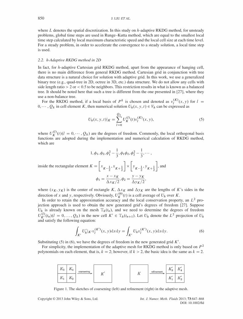
Substituting (5) in (6), we have the degrees of freedom in the new generated grid K 0.For simplicity, the implementation of the adaptive mesh for RKDG method is only based on P 2

polynomials on each element, that is, k D 2; however, if k > 2, the basic idea is the same as k D 2.

Figure 1. The sketches of coarsening (left) and refinement (right) in the adaptive mesh.



When four cells K1,K2,K3, andK4 are flagged and coarsened to a new cell K 0 (see the leftsketch in Figure 1), the new degrees of freedom are given by

U.0/K0 D

14

�U.0/K1CU

.0/K2CU

.0/K3CU

.0/K4

,

U.1/K0 D

18

�U.1/K1CU

.1/K2CU

.1/K3CU

.1/K4

C 3

8

��U

.0/K1CU

.0/K2�U

.0/K3CU

.0/K4

,

U.2/K0 D

18

�U.2/K1CU

.2/K2CU

.2/K3CU

.2/K4

C 3

8

��U

.0/K1�U

.0/K2CU

.0/K3CU

.0/K4

,

U.3/K0 D

116

�U.3/K1CU

.3/K2CU

.3/K3CU

.3/K4

C 3

16

��U

.2/K1CU

.2/K2�U

.2/K3CU

.2/K4

C 316

��U

.1/K1�U

.1/K2CU

.1/K3CU

.1/K4

C 9

16

�U.0/K1�U

.0/K2�U

.0/K3CU

.0/K4

,

U.4/K0 D

116

�U.4/K1CU

.4/K2CU

.4/K3CU

.4/K4

C 15

32

��U

.1/K1CU

.1/K2�U

.1/K3CU

.1/K4

,

U.5/K0 D

116

�U.5/K1CU

.5/K2CU

.5/K3CU

.5/K4

C 15

32

��U

.2/K1�U

.2/K2CU

.2/K3CU

.2/K4

.

(7)

When a parent cell K is flagged and refined to four child cells K1,K2,K3,K4, (see the right sketchin Figure 1), the new degrees of freedom can be defined as

U.0/

K0i

D U.0/K C aiU

.1/K C biU

.2/K C aibiU

.3/K ,

U.1/

K0i

D 12U.1/K C .�1/

iaibiU.3/K C aiU

.4/K ,

U.2/

K0i

D 12U.1/K C .�1/

i jaibi jU.3/K C biU

.5/K ,

U.3/

K0i

D 14U.3/K ,

U.4/

K0i

D 14U.4/K ,

U.5/

K0i

D 14U.5/K ,

(8)

and

ai D .�1/i 1

2, b1 D b2 D�

1

2, b3 D b4 D

1

2.i D 1, 2, 3, 4/.

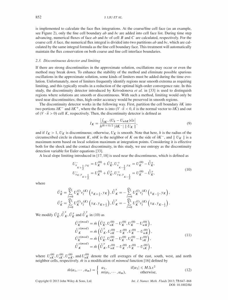
It should be noted that in the original AMR finite difference method [32], one must impose cor-rection of conservation law to make the fluxes into the fine grid across a coarse/fine cell boundary,as shown in Figure 2, equivalent to the flux out of the coarse cell after every time step advancing.However, the RKDG method is born with h-adaptive ability and can be applied in the presence ofhanging nodes. In our study, a list is used to record the cell faces, and a loop over all cell faces

Figure 2. The treatment of hanging node in the adaptive Cartesian grid.


852 J. LIU ET AL.

is implemented to calculate the face flux integrations. At the coarse/fine cell face (as an example,see Figure 2), only the fine cell boundary ab and bc are added into cell face list. During time stepadvancing, numerical fluxes of face ab and bc of cell B and C are calculated, respectively. For thecoarse cell A face, the numerical flux integral is divided into two partitions ab and bc, which are cal-culated by the same integral formula as the fine cell boundary face. This treatment will automaticallymaintain the flux conservation on both coarse and fine cell interface boundaries.

2.3. Discontinuous detector and limiting

If there are strong discontinuities in the approximate solution, oscillations may occur or even themethod may break down. To enhance the stability of the method and eliminate possible spuriousoscillations in the approximate solution, some kinds of limiters must be added during the time evo-lution. Unfortunately, most of limiters frequently identify regions near smooth extrema as requiringlimiting, and this typically results in a reduction of the optimal high-order convergence rate. In thisstudy, the discontinuity detector introduced by Krivodonova et al. in [33] is used to distinguishregions where solutions are smooth or discontinuous. With such a method, limiting would only beused near discontinuities; thus, high-order accuracy would be preserved in smooth regions.

The discontinuity detector works in the following way. First, partition the cell boundary @K intotwo portions @K� and @KC, where the flow is into .V � En < 0, En is the normal vector to @K/ and outof (V � En > 0/ cell K, respectively. Then, the discontinuity detector is defined as

IK D

ˇ̌R@K�.Uk �UnbK/ds

ˇ̌h.kC1/=2 j@K�j k UK k

, (9)

and if IK > 1, UK is discontinuous; otherwise, UK is smooth. Note that here, h is the radius of thecircumscribed circle in element K, nbK is the neighbor of K on the side of @K�, and k UK k is amaximum norm based on local solution maximum at integration points. Considering it is effectiveboth for the shock and the contact discontinuity, in this study, we use entropy as the discontinuitydetection variable for Euler equations [33].

A local slope limiting introduced in [17, 18] is used near the discontinuous, which is defined as

U�xKC

12

,yKD U

.0/K C

QU xK ,UCxK�

12

,yKD U

.0/K �

QQU xK ,

U�xK ,yKC

12

D U.0/K C

QUyK ,UCyK ,y

K�12

D U.0/K �

QQUyK ,

(10)

where

QU xK DQkPlD0

U.l/K v

.K/

l

�xKC 12

,yK

, QQUx

K D�QkPlD0

U.l/K v

.K/

l

�xK� 12

,yK

,

QUyK D

QkPlD0

U.l/K v

.K/

l

�xK ,yKC 12

, QQU

y

K D�QkPlD0

U.l/K v

.K/

l

�xK ,yK� 12

.

We modify QU xK , QQUx

K , QU yK and QQUy

K in (10) as

QUx.mod/K D Nm

�QU xK ,U .0/eK �U

.0/K ,U .0/K �U

.0/wK

,

QQUx.mod/

K D Nm�QQUx

K ,U .0/eK �U.0/K ,U .0/K �U

.0/wK

,

QUy.mod/K D Nm

�QUyK ,U .0/nK �U

.0/K ,U .0/K �U

.0/sK

,

QQUy.mod/

K D Nm�QQUy

K ,U .0/nK �U.0/K ,U .0/K �U

.0/sK

,

(11)

where U .0/eK ,U .0/sK ,U .0/wK , andU .0/nK denote the cell averages of the east, south, west, and northneighbor cells, respectively. Nm is a modification of minmod function [16] defined by

Nm.˛1, � � � ,˛m/D

²˛1, ifj˛1j6M�x2m.˛1, � � � ,˛m/, otherwise,

(12)



for the first two equations in (11), and with a change of �x to �y in the last two equations in (11).The minmod function m is defined by

m.˛1, � � � ,˛m/D

´sminij˛i j, ifs D sign.˛1/D � � � D sign.˛m/,

0, otherwise,

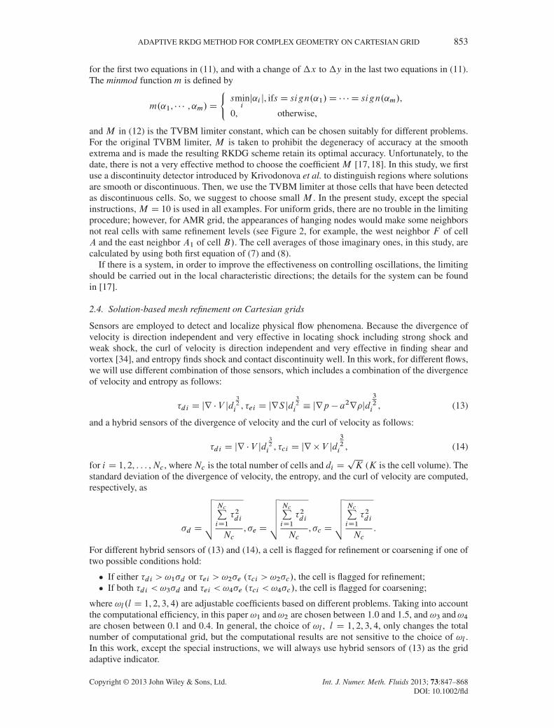
and M in (12) is the TVBM limiter constant, which can be chosen suitably for different problems.For the original TVBM limiter, M is taken to prohibit the degeneracy of accuracy at the smoothextrema and is made the resulting RKDG scheme retain its optimal accuracy. Unfortunately, to thedate, there is not a very effective method to choose the coefficient M [17, 18]. In this study, we firstuse a discontinuity detector introduced by Krivodonova et al. to distinguish regions where solutionsare smooth or discontinuous. Then, we use the TVBM limiter at those cells that have been detectedas discontinuous cells. So, we suggest to choose small M . In the present study, except the specialinstructions, M D 10 is used in all examples. For uniform grids, there are no trouble in the limitingprocedure; however, for AMR grid, the appearances of hanging nodes would make some neighborsnot real cells with same refinement levels (see Figure 2, for example, the west neighbor F of cellA and the east neighbor A1 of cell B/. The cell averages of those imaginary ones, in this study, arecalculated by using both first equation of (7) and (8).

If there is a system, in order to improve the effectiveness on controlling oscillations, the limitingshould be carried out in the local characteristic directions; the details for the system can be foundin [17].

2.4. Solution-based mesh refinement on Cartesian grids

Sensors are employed to detect and localize physical flow phenomena. Because the divergence ofvelocity is direction independent and very effective in locating shock including strong shock andweak shock, the curl of velocity is direction independent and very effective in finding shear andvortex [34], and entropy finds shock and contact discontinuity well. In this work, for different flows,we will use different combination of those sensors, which includes a combination of the divergenceof velocity and entropy as follows:

�di D jr � V jd32

i , �ei D jrS jd32

i � jrp � a2r�jd

32i , (13)

and a hybrid sensors of the divergence of velocity and the curl of velocity as follows:

�di D jr � V jd32

i , �ci D jr � V jd32i , (14)

for i D 1, 2, : : : ,Nc , whereNc is the total number of cells and di DpK (K is the cell volume). The

standard deviation of the divergence of velocity, the entropy, and the curl of velocity are computed,respectively, as

�d D

vuuutNcPiD1

�2di

Nc, �e D

vuuutNcPiD1

�2di

Nc, �c D

vuuutNcPiD1

�2di

Nc.

For different hybrid sensors of (13) and (14), a cell is flagged for refinement or coarsening if one oftwo possible conditions hold:

� If either �di > !1�d or �ei > !2�e (�ci > !2�c/, the cell is flagged for refinement;� If both �di < !3�d and �ei < !4�e (�ci < !4�c/, the cell is flagged for coarsening;

where !l.l D 1, 2, 3, 4/ are adjustable coefficients based on different problems. Taking into accountthe computational efficiency, in this paper !1 and!2 are chosen between 1.0 and 1.5, and !3 and!4are chosen between 0.1 and 0.4. In general, the choice of !l , l D 1, 2, 3, 4, only changes the totalnumber of computational grid, but the computational results are not sensitive to the choice of !l .In this work, except the special instructions, we will always use hybrid sensors of (13) as the gridadaptive indicator.


854 J. LIU ET AL.

3. BOUNDARY TREATMENT

It has been shown that the DG method for flow problems is highly sensitive to the accuracy of theboundary representation [28]. In order to cure the large errors arising near the boundary and reducethe pollution of the solution inside the domain, one often needs to use curved elements, whichlargely enhance the difficulties of geometry processing. Furthermore, in practical simulations, acurved geometry is often approximated by a straight-sided polygon. This produces larger numericalboundary error near the body boundary surface. This error may dominate the discretization errorof the scheme and lead to a wrong solution. In this study, the body is immersed into the Cartesianvolume grid, in other words, the quality of grid is not so good near the body boundary. Therefore,care should be taken when we deal with a complex geometry. In this paper, we adopt the idea ofghost cell immersed boundary method to treat nonconforming boundary for the RKDG method.

Recently, Dadone et al. [4] use finite difference method to present some systemic results abouta novel GCM for static body on Cartesian grid. In this paper, we extend it to treat the boundary inRKDG method on Cartesian grid. The basic idea is that the ghost cell values are developed on thebasis of an assumption of flow field model in the vicinity of the wall consisting of a vortex flow withlocally symmetric distribution of entropy S and the total enthalpy H per unit mass along a surfacenormal and also take into account the effect of curvature. If R is the local radius of curvature of thewall and VEt is the velocity component tangential to the body surface, then the flow model satisfiesthe normal momentum equation

@p

@EnD��

.VEt /2

R, (15)

the nonpenetration boundary condition VEn D V�EnD 0, and enforces antisymmetric normal derivative@S=@En and @H=@En along the surface normal to the body in the vicinity of the body. These entropyand total enthalpy distributions will produce zero normal derivatives when the flow is irrotational.Using finite difference scheme, the method has shown to produce superior accuracy compared withthe classical surface boundary condition by Dadone et al. in [4]. In view of many good charac-ters, the method has also been successfully used in second order accuracy finite volume method atbody-fitted unstructured grid by Wang and Sun in [35].

In order to implement the ghost cell methodology for an immersed boundary, we need to proceedby first identifying the cells whose centers are inside the solid and determine the ghost cells. Solidcells can be identified by ray tracing. Because the stencil of RKDG is compact and only demand thenearest neighbor cells, hence, we only need to identify the closest row of solid cells near the bodysurface as the ghost cells (gc). Those cells are shown in Figure 3. Following this, we should derive ascheme that allows us to calculate the value of the variables at each of these ghost cell centers such

Solid body

fluid cell

gc

ip1gc1

gc gc gcgc

ip

Figure 3. 2D schematic describing ghost cell method used in the current solver.



that the boundary conditions on the immersed boundary in the vicinity of the ghost cell are satisfied.Here, the GCM for two-dimensional inviscid flow on Cartesian grids use the following equations:

pgc D pip � �ip

V 2Etip

R�n,

�gc D �ip

�pgc

pip

� 1�

,

V 2EtgcD V 2

EtipC

2�

� � 1

�pip

�ip�pgc

�gc

�,

VEngc D�VEnip ,

(16)

where ip denotes the image point corresponding to his ghost cell (gc) and �n indicates the distancebetween the ip and gc. Then, the nonpenetration boundary conditions are satisfied automatically.

It is well known that the values at the image points ip can be achieved by some interpolationformulas with the surrounding fluid cells. Clearly, using any form of polynomial interpolation tech-niques across strong discontinuities will result in interpolation errors and may produce pseudoextremes. However, the inverse distance weighting interpolation normally neither generates anynew extreme nor produces pseudo oscillations. In the DG frame, DG solutions are available in allthe fluid cells, and one can use solution polynomial to interpolate the values at the reflected imagepoints. However, it should be noted that in the presented boundary treatment, one situation will beencountered, which is the image point located in the ghost cell itself; see for instance the point ip1shown in Figure 3. In this ghost cell, there is no DG solution polynomial. Of course, one can useDG solution in some neighboring fluid cells to extrapolate it. However, there are several fluid cellsthat are near this ghost cell. In this case, one must give a choice for using the neighboring cells.For convenience, it was chosen all the surrounding fluid cell averages to interpolate the value at thereflected point. It could also be the case that the surrounding interpolation stencil for image pointof ghost cell contains other ghost cells. So in this work, for simplicity and robustness, the inversedistance weighting interpolation formula [5] at the image point is used.

In order to evaluate the pressure pgc at a ghost cell in the first equation of (16), for an arbitrarycurved boundary, it is also needed to estimate the local curvature. Here, we adopt the method sug-gested by Wang and Sun [35] for two-dimensional flow. Let us consider a curved boundary as shownin Figure 4. To estimate the curvature for body surface A�B , first we use A�B and the point to theleft of the boundary face (point Lft) to make one estimate, and then we use A�B and the right pointRgt to perform the other estimate. Then, the final radius can be obtained by a simple average of thetwo estimates. The local averaged radius is used as the final approximation of the local curvature.However, if either point A or B is a sharp corner, then the estimate would be only calculated by thethree points to avoid the sharp corner.

Recently, Krivodonova and Berger [29] presented a new boundary treatment on body-fittedunstructured grid to make the numerical velocity at every boundary integration point to coincidewith the streamline direction near the body surface, that is, to be orthogonal to the ‘true’ approxi-mated geometrical boundary rather than to the computational boundary. They impose the followingcondition at every integration point:

V � EN D 0, (17)

Lft

A

BRgt

Figure 4. Estimation of local curvature for 2D body.


856 J. LIU ET AL.

n

N

gc

solid

fluid

approximate wallboundary

computational boundary

Figure 5. Modification of the normal velocity.

in a small vicinity to the surface, where EN is the unit normal to the physical geometry. Usingthis technique, they did not use curved elements in body-fitted unstructured grid and obtained veryaccurate results.

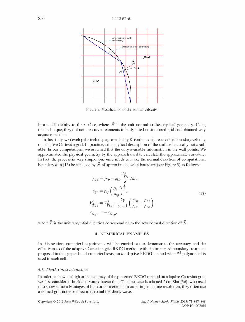
In this study, we develop the technique presented by Krivodonova to resolve the boundary velocityon adaptive Cartesian grid. In practice, an analytical description of the surface is usually not avail-able. In our computations, we assumed that the only available information is the wall points. Weapproximated the physical geometry by the approach used to calculate the approximate curvature.In fact, the process is very simple; one only needs to make the normal direction of computationalboundary En in (16) be replaced by EN of approximated solid boundary (see Figure 5) as follows:

pgc D pip � �ip

V 2ET ip

R�n,

�gc D �ip

�pgc

pip

� 1�

,

V 2ETgcD V 2

ET ipC

2�

� � 1

�pip

�ip�pgc

�gc

�,

V ENgc D�V ENip ,

(18)

where ET is the unit tangential direction corresponding to the new normal direction of EN .

4. NUMERICAL EXAMPLES

In this section, numerical experiments will be carried out to demonstrate the accuracy and theeffectiveness of the adaptive Cartesian grid RKDG method with the immersed boundary treatmentproposed in this paper. In all numerical tests, an h-adaptive RKDG method with P 2 polynomial isused in each cell.

4.1. Shock vortex interaction

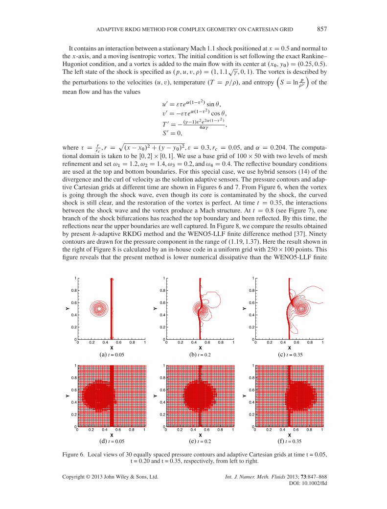
In order to show the high order accuracy of the presented RKDG method on adaptive Cartesian grid,we first consider a shock and vortex interaction. This test case is adapted from Shu [36], who usedit to show some advantages of high order methods. In order to gain a fine resolution, they often usea refined grid in the x-direction around the shock wave.



It contains an interaction between a stationary Mach 1.1 shock positioned at x D 0.5 and normal tothe x-axis, and a moving isentropic vortex. The initial condition is set following the exact Rankine–Hugoniot condition, and a vortex is added to the main flow with its center at .x0,y0/D .0.25, 0.5/.The left state of the shock is specified as .p,u, v, �/ D .1, 1.1

p� , 0, 1/. The vortex is described by

the perturbations to the velocities .u, v/, temperature .T D p=�/, and entropy�S D ln p

��

of the

mean flow and has the values

u0 D "�e˛.1��2/ sin ,

v0 D�"�e˛.1��2/ cos ,

T 0 D� .��1/"2e2˛.1��

2/

4˛�,

S 0 D 0,

where � D rrc

, r Dp.x � x0/2C .y � y0/2, " D 0.3, rc D 0.05, and ˛ D 0.204. The computa-

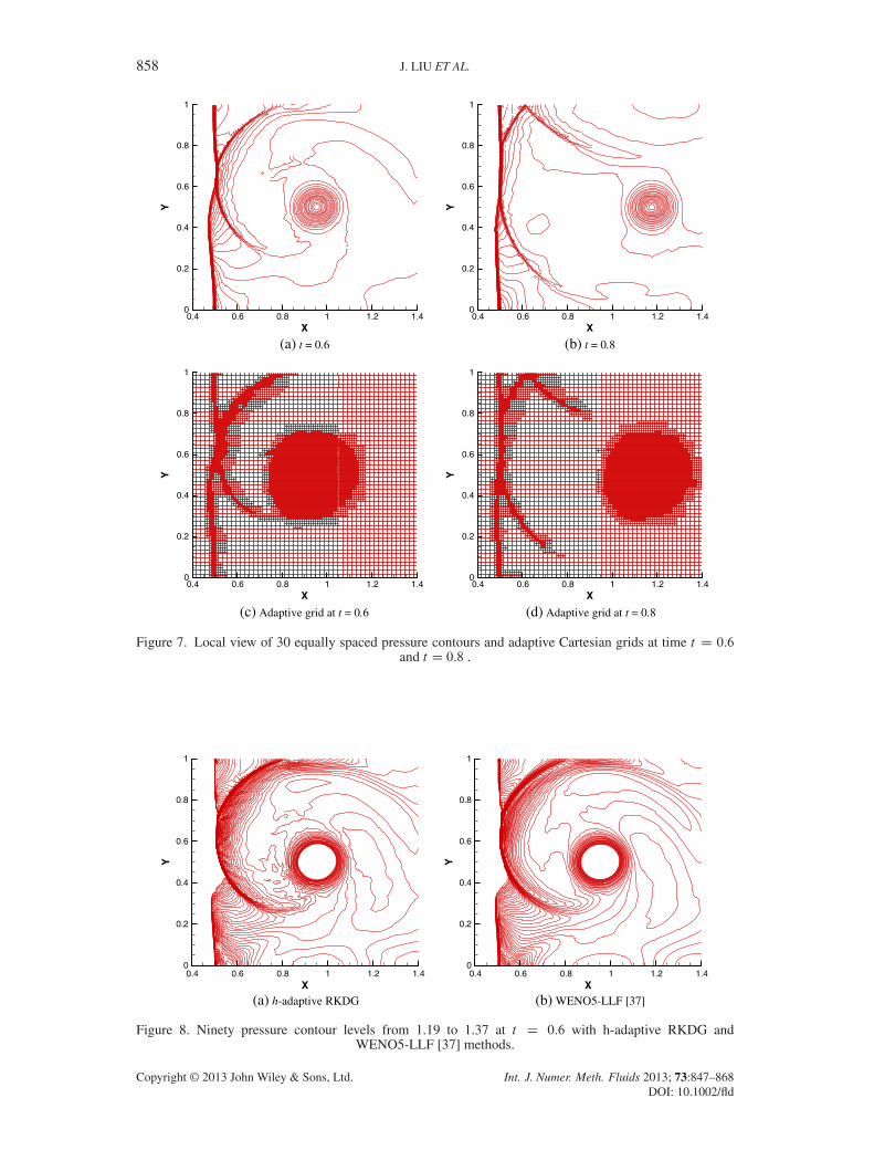
tional domain is taken to be Œ0, 2 � Œ0, 1. We use a base grid of 100 � 50 with two levels of meshrefinement and set !1 D 1.2,!2 D 1.4,!3 D 0.2, and!4 D 0.4. The reflective boundary conditionsare used at the top and bottom boundaries. For this special case, we use hybrid sensors (14) of thedivergence and the curl of velocity as the solution adaptive sensors. The pressure contours and adap-tive Cartesian grids at different time are shown in Figures 6 and 7. From Figure 6, when the vortexis going through the shock wave, even though its core is contaminated by the shock, the curvedshock is still clear, and the restoration of the vortex is perfect. At time t D 0.35, the interactionsbetween the shock wave and the vortex produce a Mach structure. At t D 0.8 (see Figure 7), onebranch of the shock bifurcations has reached the top boundary and been reflected. By this time, thereflections near the upper boundaries are well captured. In Figure 8, we compare the results obtainedby present h-adaptive RKDG method and the WENO5-LLF finite difference method [37]. Ninetycontours are drawn for the pressure component in the range of .1.19, 1.37/. Here the result shown inthe right of Figure 8 is calculated by an in-house code in a uniform grid with 250� 100 points. Thisfigure reveals that the present method is lower numerical dissipative than the WENO5-LLF finite

X

Y

0 0.2 0.4 0.6 0.8 10

0.2

0.4

0.6

0.8

1

(a) t = 0.05X

Y

0 0.2 0.4 0.6 0.8 10

0.2

0.4

0.6

0.8

1

(b) t = 0.2

X

Y

0 0.2 0.4 0.6 0.8 10

0.2

0.4

0.6

0.8

1

(c) t = 0.35

X

Y

0 0.2 0.4 0.6 0.8 10

0.2

0.4

0.6

0.8

1

(d) t = 0.05X

Y

0 0.2 0.4 0.6 0.8 10

0.2

0.4

0.6

0.8

1

(e) t = 0.2X

Y

0 0.2 0.4 0.6 0.8 10

0.2

0.4

0.6

0.8

1

(f) t = 0.35

Figure 6. Local views of 30 equally spaced pressure contours and adaptive Cartesian grids at time t = 0.05,t = 0.20 and t = 0.35, respectively, from left to right.


858 J. LIU ET AL.

X

Y

0.4 0.6 0.8 1 1.2 1.40

0.2

0.4

0.6

0.8

1

(a) t = 0.6

X

Y

0.4 0.6 0.8 1 1.2 1.40

0.2

0.4

0.6

0.8

1

(b) t = 0.8

X

Y

0.4 0.6 0.8 1 1.2 1.40

0.2

0.4

0.6

0.8

1

(c) Adaptive grid at t = 0.6

X

Y

0.4 0.6 0.8 1 1.2 1.40

0.2

0.4

0.6

0.8

1

(d) Adaptive grid at t = 0.8

Figure 7. Local view of 30 equally spaced pressure contours and adaptive Cartesian grids at time t D 0.6and t D 0.8 .

X

Y

0.4 0.6 0.8 1 1.2 1.40

0.2

0.4

0.6

0.8

1

(a) h-adaptive RKDGX

Y

0.4 0.6 0.8 1 1.2 1.40

0.2

0.4

0.6

0.8

1

(b) WENO5-LLF [37]

Figure 8. Ninety pressure contour levels from 1.19 to 1.37 at t D 0.6 with h-adaptive RKDG andWENO5-LLF [37] methods.



difference method [37] and the solution has some slight oscillations. Because of the utilization ofAMR, the shock is more thin than WENO5-LLF finite difference method.

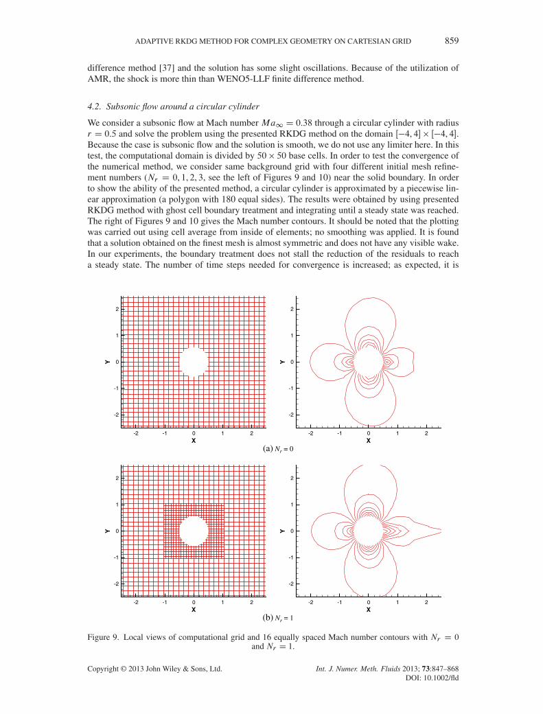
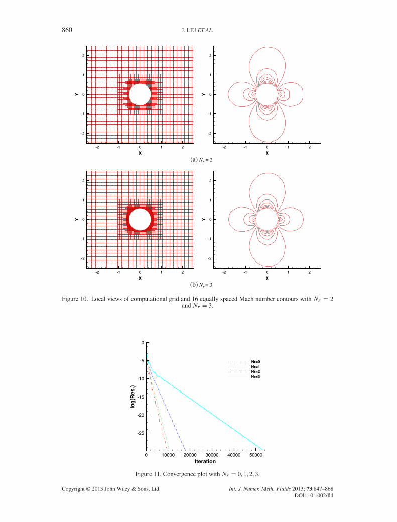
4.2. Subsonic flow around a circular cylinder

We consider a subsonic flow at Mach number Ma1 D 0.38 through a circular cylinder with radiusr D 0.5 and solve the problem using the presented RKDG method on the domain Œ�4, 4� Œ�4, 4.Because the case is subsonic flow and the solution is smooth, we do not use any limiter here. In thistest, the computational domain is divided by 50 � 50 base cells. In order to test the convergence ofthe numerical method, we consider same background grid with four different initial mesh refine-ment numbers (Nr D 0, 1, 2, 3, see the left of Figures 9 and 10) near the solid boundary. In orderto show the ability of the presented method, a circular cylinder is approximated by a piecewise lin-ear approximation (a polygon with 180 equal sides). The results were obtained by using presentedRKDG method with ghost cell boundary treatment and integrating until a steady state was reached.The right of Figures 9 and 10 gives the Mach number contours. It should be noted that the plottingwas carried out using cell average from inside of elements; no smoothing was applied. It is foundthat a solution obtained on the finest mesh is almost symmetric and does not have any visible wake.In our experiments, the boundary treatment does not stall the reduction of the residuals to reacha steady state. The number of time steps needed for convergence is increased; as expected, it is

X

Y

-2 -1 0 1 2

-2

-1

0

1

2

X

Y

-2 -1 0 1 2

-2

-1

0

1

2

(a) Nr = 0

X

Y

-2 -1 0 1 2

-2

-1

0

1

2

X

Y

-2 -1 0 1 2

-2

-1

0

1

2

(b) Nr = 1

Figure 9. Local views of computational grid and 16 equally spaced Mach number contours with Nr D 0and Nr D 1.


860 J. LIU ET AL.

X

Y

-2 -1 0 1 2

-2

-1

0

1

2

X

Y

-2 -1 0 1 2

-2

-1

0

1

2

(a) Nr = 2

X

Y

-2 -1 0 1 2

-2

-1

0

1

2

X

Y

-2 -1 0 1 2

-2

-1

0

1

2

(b) Nr = 3

Figure 10. Local views of computational grid and 16 equally spaced Mach number contours with Nr D 2and Nr D 3.

Iteration

log

(Res

.)

0 10000 20000 30000 40000 50000

-25

-20

-15

-10

-5

0

Nr=0Nr=1Nr=2Nr=3

Figure 11. Convergence plot with Nr D 0, 1, 2, 3.



Table I. L1=L2 errors in entropy for the circular cylinder.

GCM (Equation (16)) GCM (Equation (18))

Nr L1."ent/ L2."ent/ L1."ent/ L2."ent/

0 3.4276e-02 1.4776e-02 3.3800e-02 1.4307e-021 1.3535e-02 7.7288e-03 1.3397e-02 7.6334e-032 4.2376e-03 1.3669e-03 4.0243e-03 1.3506e-033 1.7150e-03 3.7130e-04 1.5812e-03 3.3752e-04

in inverse proportion to the reduced element size (h-refinement). The convergence histories withdifferent grids are illustrated in Figure 11.

To show the convergences of the proposed method, we also measure the L2 and L1 errors inentropy "ent defined as

"ent Dp

p1

��

�1

��1 (19)

where p1 and �1 are pressure and density of the free stream, respectively. Note that the entropyproduction serves as a good criterion to measure accuracy of the numerical solutions, because theflow under consideration is isentropic. The results with h-refinement are shown in Table I. Clearly,Table I shows that the modified version (18) of GCM produces slightly less errors than the originalone (16). For instance, the modified version GCM method has about a 10% reduction in L2 errorand an 8% reduction in L1 error (in the finest mesh) compared with the ones in the GCM method.

4.3. Shock diffraction over a circular cylinder

This example concerns the shock/cylinder interaction problem, which is one of the well-studiedtest cases in the literature [10, 11, 38]. The flow consists of a planar shock moving at Ma D 2.81and impinging on a solid cylinder. The state variables at the right of the shock at time t D 0 are

.�,p,u, v/ D�1, 1�

, 0, 0

, and quantities at the left of the shock are computed from the ones at the

right side and the Mach number of shock wave using classical shock relations. The computationaldomain is Œ0, 1 � Œ�0.5, 0.5, which is similar to the case presented in [10]. Wall boundary condi-tions are used for the top and bottom, and the Neumann condition is used for the outlet. At the inlet,a Dirichlet condition corresponding to a Mach 2.81 shock is enforced. The circular obstacle witha radius of 0.105 was positioned at x D 0.5 and y D 0. The initial discontinuity was located atx D 0.385.

The simulations were performed with a coarse base mesh of size �x D �y D 180

and four lev-els of mesh refinement with !1 D 1.1,!2 D 1.5,!3 D !4 D 0.3 was selected. Figure 12 showsthe adaptive grids and the density contour images from the simulation of the shock and cylinderinteraction at different times t D 0.2 and t D 0.5. The evolution of diffraction process includesregular reflection, transition to Mach reflection, complex wake/shock, and shock/shock interac-tions. The contact discontinuities, upper and lower triple points, complex wake structure, and theMach systems are correctly reproduced by the present simulation. Furthermore, thanks to the highorder accuracy RKDG method, the onset of instability was found behind the cylinder in the right ofFigure 12. The computed trajectories of the upper triple point (denoted by AMRDG) are depicted inFigure 13. The present simulation agrees well with the numerical calculation presented in [10] andthe experimental correction obtained in [39, 40].

4.4. Supersonic flow around a triangle

In this section, we consider the same example presented in [5, 38], where a supersonic flow past asolid body of triangular shape with height h D 0.5 and half angle D 20 deg, as shown on theleft of Figure 14. The free stream Mach number is 2. In this geometry, a special procedure will beencountered, which is the problem of multivalued ghost points. It is often found near unresolved


862 J. LIU ET AL.

(a) t = 0.2

(b) t = 0.5

Figure 12. Adaptive grids and density pseudocolor images for a Mach 2.81 shock wave diffracting off astationary cylindrical obstacle, computed on a base mesh of size �x D �y D 1

80with four levels of mesh

refinement at time t D 0.2 and t D 0.5.

X

Y

0.4 0.5 0.6 0.7 0.8 0.9 10

0.1

0.2

0.3

0.4

0.5

AMRDGExp.Ref.

Figure 13. Comparison of triple point trajectory.



h

theta

X

Y

-0.5 0 0.5 1 1.5-1

-0.5

0

0.5

1

Figure 14. Geometrical configuration for oblique shock wave analysis and the local view of the adaptiveCartesian grid.

thin surfaces and sharp corners, such as the cases at the sharp trailing edge of an airfoil or near theapex of triangle as shown in Figure 14. At sharp corners, one cell center inside the geometry may bethe ghost cell center for one side of the corner surface, as well as for the other sides. Also, a ghostcell center pertaining to one side of a corner surface may be located inside the flow field on the otherside of the corner. To handle this case, we first find the fluid cells, which are needed for multiplevalued ghost points, and then set flags. Generally speaking, the ghost boundary conditions are givenbefore time evolution. In this special situation, the multiple valued ghost points are evaluated duringthe time evolution, which accords to the fluid cell to find the corresponding ghost cell value. Therest of fluid cells are computed as usual. The advantage of this approach is that there is no need toallocate new memory to save the values on the multiple valued ghost points.

The problem was solved by the present adaptive ghost cell Cartesian grid method on the domainŒ�4, 5.5 � Œ�4.5, 4.5. Initial grids (the domain is divided by 60 � 60 cells) have been refined sixtimes near the body, then three levels of grid refinements are implemented during solution processwith !1 D 1.1,!2 D 1.5,!3 D !4 D 0.3. The final mesh is shown on the right of Figure 14.The total number of grid points is 31,475. Figure 15 shows the Mach number contours and residualhistory obtained by the presented method. The positions of the attached shock waves are clearlyindicated in the plots.

Iteration

log

(Res

.)

0 10000 20000 30000 40000-7

-6

-5

-4

-3

-2

X

Y

-0.5 0 0.5 1 1.5-1

-0.5

0

0.5

1

MA

3.83.63.43.232.82.62.42.221.81.61.41.210.80.60.40.2

Figure 15. Mach number contours and residual history.


864 J. LIU ET AL.

An oblique shock can be attached or detached depending on the values of the deflection angle and the upstream Mach number M1. If the shock is attached to the triangle, its angle with thehorizontal, ˇ, can be computed through the following relationship given by [38]:

tan D 2 cotˇ

"M 21 sin2 ˇ � 1

M 21 .� C cos 2ˇ/C 2

#. (20)

For M1 D 2 and D 20 deg, the angle ˇ would be ˇ D 53.46 deg from Equation (20). Boironet al. [38] presented numerical values of ˇ by using a high-resolution penalization method to solveviscous Navier–Stokes equations. Their numerical values of ˇ are 54.13 deg on 5122 grid points,53.70 deg on 10242 grid points, and 53.56 deg on 15362 grid points, respectively. In our results forthe Euler equations on the 31,475 grid points, which is much less than their grid points, the meanshock angle of ˇ is about ˇ � 52.69 deg, which is comparable with theirs.

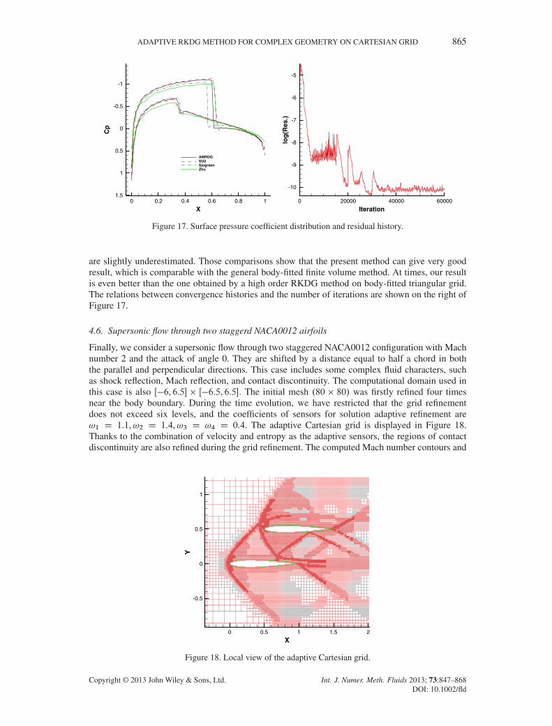
4.5. Transonic flow past a NACA0012 airfoil

Now, let us consider an application of the present method on an airfoil. Because the airfoil has asharp trailing edge, it is difficult to define the ghost cell boundary as the aforesaid triangle.

In the transonic flow computation, the Mach number is 0.8 and the angle of attack 1.25 deg aroundthe NACA0012 airfoil (chord = 1). The computational domain for this case is Œ�6, 6.5� Œ�6.5, 6.5.The initial mesh .80 � 80/ was first refined four times near the body boundary. Four levels ofsolution-based refinement are carried out during the time evolution. The mesh is shown in the leftof Figure 16. It should be noted that a sensor of the divergence of velocity �d is only used inthe process of solution-based refinement. The coefficients of sensors for adaptive refinement are!1 D 1.1 and!3 D 0.2. The density contours are shown on the right of Figure 16. The calcu-lated pressure coefficient denoted by AMRDG is plotted on the left of Figure 17. The figure alsogives a comparison with some references. In Figure 17, the result flagged by SU2 is calculated byStanford University unstructured code SU2 [41], which uses a second order finite volume schemeon body-fitted unstructured grid to discretize the Euler equations. As shown in Figure 17, becauseof the usage of adaptive Cartesian grid, except that the calculated shock is more thin than SU2, thepresent result matches very well with the one calculated by SU2; both the strong shock and the weakshock are well resolved, and the positions of shock are also well located. Sj ö green and Peterssonrecently developed an embedded boundary method to solve Euler equations on Cartesian grid [2].Using 1200�1200 grids, they obtained the pressure coefficients as shown in Figure 17. Their resultslightly misses the position of the shock. We also compared our result with the one calculated bya body-fitted triangular grid RKDG method with WENO limiter by Zhu et al. in [42]. From thesame figure, we find that heir result gives the right position of shock, but their pressure coefficients

X

Y

0 0.5 1 1.5

-0.5

0

0.5

X

Y

-1 -0.5 0 0.5 1 1.5 2

-1

-0.5

0

0.5

1

1.5

Figure 16. Adaptive Cartesian grid and 20 equally spaced density contours.



X

Cp

0 0.2 0.4 0.6 0.8 1

-1

-0.5

0

0.5

1

1.5

AMRDGSU2SjogreenZhu

Iteration

log

(Res

.)

0 20000 40000 60000

-10

-9

-8

-7

-6

-5

Figure 17. Surface pressure coefficient distribution and residual history.

are slightly underestimated. Those comparisons show that the present method can give very goodresult, which is comparable with the general body-fitted finite volume method. At times, our resultis even better than the one obtained by a high order RKDG method on body-fitted triangular grid.The relations between convergence histories and the number of iterations are shown on the right ofFigure 17.

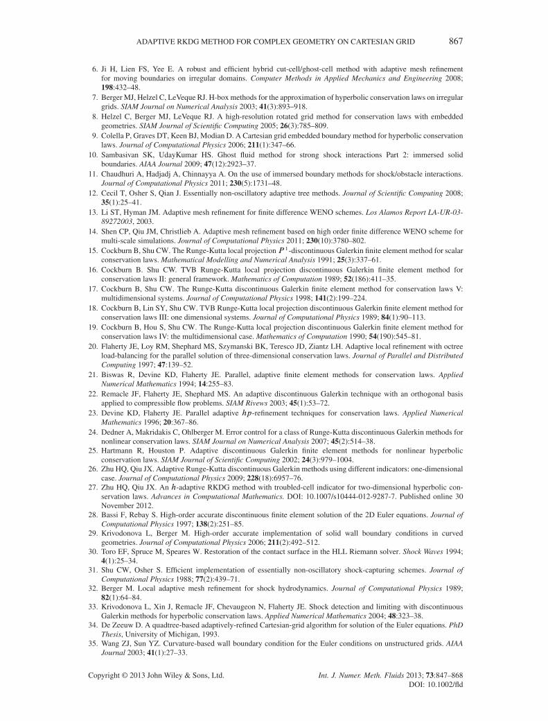
4.6. Supersonic flow through two staggerd NACA0012 airfoils

Finally, we consider a supersonic flow through two staggered NACA0012 configuration with Machnumber 2 and the attack of angle 0. They are shifted by a distance equal to half a chord in boththe parallel and perpendicular directions. This case includes some complex fluid characters, suchas shock reflection, Mach reflection, and contact discontinuity. The computational domain used inthis case is also Œ�6, 6.5 � Œ�6.5, 6.5. The initial mesh .80 � 80/ was firstly refined four timesnear the body boundary. During the time evolution, we have restricted that the grid refinementdoes not exceed six levels, and the coefficients of sensors for solution adaptive refinement are!1 D 1.1,!2 D 1.4,!3 D !4 D 0.4. The adaptive Cartesian grid is displayed in Figure 18.Thanks to the combination of velocity and entropy as the adaptive sensors, the regions of contactdiscontinuity are also refined during the grid refinement. The computed Mach number contours and

X

Y

0 0.5 1 1.5 2

-0.5

0

0.5

1

Figure 18. Local view of the adaptive Cartesian grid.


866 J. LIU ET AL.

X

Y

-0.5 0 0.5 1 1.5 2 2.5

-1.5

-1

-0.5

0

0.5

1

1.5

X

Cp

0 0.5 1 1.5

-0.5

0

0.5

1

1.5

2

AMRDGLi

Figure 19. Local view of the Mach number contours and the surface pressure coefficient distribution.

the pressure coefficient distribution on the surface are shown in Figure 19. Clearly, the contact andshock wave are captured and resolved very well. It is also noted that the pressure coefficients matchwell with the one calculated by a nonet-Cartesian grid method [43].

5. CONCLUSION

The ghost cell Cartesian grid method provides an efficient and flexible alternative to the traditionalbody-fitted grid techniques. The RKDG method is an efficient high order scheme, which can easilydeal with grid refinement and retain local conservation even in the case of hang node. In this paper,an h-adaptive Cartesian grid RKDG method is developed. A discontinuous detector and limitingtechnique is used to suppress oscillation, and a solution-based grid adaptive method with hybridsensors is used during the grid refinement. In order to solve flow with complex geometry, in thispaper, an h-adaptive Cartesian grid RKDG method with ghost cell immersed boundary methodhas been successfully developed and used to simulate steady and unsteady problems of the Eulerequations. Although the boundary treatment is not conservative and at most in second order accu-racy, numerical results show that the present method can achieve correct shock positions, highresolution, and some correct physical characters. It is demonstrated that the present method is veryeffective.

ACKNOWLEDGEMENTS

The research was partially supported by the National Science Foundation of China (No.11102179, No.91230110), DMU PhD Studentship (De Montfort University, UK), and Science Foundation of Institutionsof Higher Education of Jiangsu Province (No. 11KJB110016), China.

REFERENCES

1. Yang G, Causon DM, Ingram DM, Saunders R, Batten P. A Cartesian cut cell method for compressible flows part A:static body problems. Aeronautical Journal 1997; 101(1001):47–56.

2. Sj ö green B, Petersson N. A Cartesian embedded boundary method for hyperbolic conservation laws. Communica-tions in Computational Physics 2007; 2(6):1199–219.

3. Forrer H, Jeltsch R. A higher-order boundary treatment for Cartesian-grid methods. Journal of ComputationalPhysics 1998; 140(2):259–77.

4. Dadone A, Grossman B. Ghost-cell method for inviscid two-dimensional flows on Cartesian grids. AIAA Journal2004; 42(12):2499–507.

5. Liu JM, Zhao N, Hu O. The ghost cell method and its applications for inviscid compressible flow on adaptive treeCartesian grids. Advances in Applied Mathematics and Mechanics 2009; 1(5):664–82.



6. Ji H, Lien FS, Yee E. A robust and efficient hybrid cut-cell/ghost-cell method with adaptive mesh refinementfor moving boundaries on irregular domains. Computer Methods in Applied Mechanics and Engineering 2008;198:432–48.

7. Berger MJ, Helzel C, LeVeque RJ. H-box methods for the approximation of hyperbolic conservation laws on irregulargrids. SIAM Journal on Numerical Analysis 2003; 41(3):893–918.

8. Helzel C, Berger MJ, LeVeque RJ. A high-resolution rotated grid method for conservation laws with embeddedgeometries. SIAM Journal of Scientific Computing 2005; 26(3):785–809.

9. Colella P, Graves DT, Keen BJ, Modian D. A Cartesian grid embedded boundary method for hyperbolic conservationlaws. Journal of Computational Physics 2006; 211(1):347–66.

10. Sambasivan SK, UdayKumar HS. Ghost fluid method for strong shock interactions Part 2: immersed solidboundaries. AIAA Journal 2009; 47(12):2923–37.

11. Chaudhuri A, Hadjadj A, Chinnayya A. On the use of immersed boundary methods for shock/obstacle interactions.Journal of Computational Physics 2011; 230(5):1731–48.

12. Cecil T, Osher S, Qian J. Essentially non-oscillatory adaptive tree methods. Journal of Scientific Computing 2008;35(1):25–41.

13. Li ST, Hyman JM. Adaptive mesh refinement for finite difference WENO schemes. Los Alamos Report LA-UR-03-89272003, 2003.

14. Shen CP, Qiu JM, Christlieb A. Adaptive mesh refinement based on high order finite difference WENO scheme formulti-scale simulations. Journal of Computational Physics 2011; 230(10):3780–802.

15. Cockburn B, Shu CW. The Runge-Kutta local projectionP 1-discontinuous Galerkin finite element method for scalarconservation laws. Mathematical Modelling and Numerical Analysis 1991; 25(3):337–61.

16. Cockburn B. Shu CW. TVB Runge-Kutta local projection discontinuous Galerkin finite element method forconservation laws II: general framework. Mathematics of Computation 1989; 52(186):411–35.

17. Cockburn B, Shu CW. The Runge-Kutta discontinuous Galerkin finite element method for conservation laws V:multidimensional systems. Journal of Computational Physics 1998; 141(2):199–224.

18. Cockburn B, Lin SY, Shu CW. TVB Runge-Kutta local projection discontinuous Galerkin finite element method forconservation laws III: one dimensional systems. Journal of Computational Physics 1989; 84(1):90–113.

19. Cockburn B, Hou S, Shu CW. The Runge-Kutta local projection discontinuous Galerkin finite element method forconservation laws IV: the multidimensional case. Mathematics of Computation 1990; 54(190):545–81.

20. Flaherty JE, Loy RM, Shephard MS, Szymanski BK, Teresco JD, Ziantz LH. Adaptive local refinement with octreeload-balancing for the parallel solution of three-dimensional conservation laws. Journal of Parallel and DistributedComputing 1997; 47:139–52.

21. Biswas R, Devine KD, Flaherty JE. Parallel, adaptive finite element methods for conservation laws. AppliedNumerical Mathematics 1994; 14:255–83.

22. Remacle JF, Flaherty JE, Shephard MS. An adaptive discontinuous Galerkin technique with an orthogonal basisapplied to compressible flow problems. SIAM Rivews 2003; 45(1):53–72.

23. Devine KD, Flaherty JE. Parallel adaptive hp-refinement techniques for conservation laws. Applied NumericalMathematics 1996; 20:367–86.

24. Dedner A, Makridakis C, Ohlberger M. Error control for a class of Runge-Kutta discontinuous Galerkin methods fornonlinear conservation laws. SIAM Journal on Numerical Analysis 2007; 45(2):514–38.

25. Hartmann R, Houston P. Adaptive discontinuous Galerkin finite element methods for nonlinear hyperbolicconservation laws. SIAM Journal of Scientific Computing 2002; 24(3):979–1004.

26. Zhu HQ, Qiu JX. Adaptive Runge-Kutta discontinuous Galerkin methods using different indicators: one-dimensionalcase. Journal of Computational Physics 2009; 228(18):6957–76.

27. Zhu HQ, Qiu JX. An h-adaptive RKDG method with troubled-cell indicator for two-dimensional hyperbolic con-servation laws. Advances in Computational Mathematics. DOI: 10.1007/s10444-012-9287-7. Published online 30November 2012.

28. Bassi F, Rebay S. High-order accurate discontinuous finite element solution of the 2D Euler equations. Journal ofComputational Physics 1997; 138(2):251–85.

29. Krivodonova L, Berger M. High-order accurate implementation of solid wall boundary conditions in curvedgeometries. Journal of Computational Physics 2006; 211(2):492–512.

30. Toro EF, Spruce M, Speares W. Restoration of the contact surface in the HLL Riemann solver. Shock Waves 1994;4(1):25–34.

31. Shu CW, Osher S. Efficient implementation of essentially non-oscillatory shock-capturing schemes. Journal ofComputational Physics 1988; 77(2):439–71.

32. Berger M. Local adaptive mesh refinement for shock hydrodynamics. Journal of Computational Physics 1989;82(1):64–84.

33. Krivodonova L, Xin J, Remacle JF, Chevaugeon N, Flaherty JE. Shock detection and limiting with discontinuousGalerkin methods for hyperbolic conservation laws. Applied Numerical Mathematics 2004; 48:323–38.

34. De Zeeuw D. A quadtree-based adaptively-refined Cartesian-grid algorithm for solution of the Euler equations. PhDThesis, University of Michigan, 1993.

35. Wang ZJ, Sun YZ. Curvature-based wall boundary condition for the Euler conditions on unstructured grids. AIAAJournal 2003; 41(1):27–33.


868 J. LIU ET AL.

36. Shu CW. Essentially non-oscillatory and weighted essentially non-oscillatory schemes for hyperbolic conservationlaws. NASA CR-97-206253, 1997.

37. Balsara DS, Shu CW. Monotonicity preserving weighted essentially non-oscillatory schemes with increasingly highorder of accuracy. Journal of Computational Physics 2000; 160(2):405–52.

38. Boiron O, Chiavassa G, Donat R. A high-resolution penalization method for large Mach number flows in the presenceof obstacles. Computers & Fluids 2009; 38(3):703–14.

39. Ripley R, Lien F, Yovanovich M. Numerical simulation of shock diffraction on unstructured meshes. Computers &Fluids 2006; 35(10):1420–31.

40. Kaca J. An Interferometric investigation of the diffraction of a planar shock wave over a semicircular cylinder. Instfor Aerospace Studies TR 269, Univ of Toronto, 1988.

41. Palacios F, Alonso JJ, Duraisamy K, Colonno MR, Aranake AC, Campos A, Copeland SR, Economon TD, LonkarAK, Lukaczyk TW, Taylor TWR. Stanford University Unstructured (SU2): An open-source integrated computa-tional environment for multi-physics simulation and design. AIAA Paper 2013-0287, 51st AIAA Aerospace SciencesMeeting and Exhibit, Grapevine, Texas, USA, January 7th–10th, 2013.

42. Zhu J, Qiu JX, Shu CW, Dumbser M. Runge-Kutta discontinuous Galerkin method using WENO limiters II:unstructured meshes. Journal of Computational Physics 2008; 227(9):4330–4353.

43. Li K, Wu ZN. Nonet-Cartesian grid method for shock flow computations. Journal of Scientific Computing 2004;20(3):303–29.


adaptive runge–kutta discontinuous galerkin method...

Documents