adaptive power transformer lifetime predictions through ... · transformer loading capability and...

IEEE TRANSACTIONS ON INDUSTRIAL ELECTRONICS

Adaptive Power Transformer Lifetime Predictionsthrough Machine Learning & Uncertainty

Modelling in Nuclear Power PlantsJose Ignacio Aizpurua, Member, IEEE,Stephen D. J. McArthur, Fellow, IEEE,Brian G.

Stewart, Member, IEEE,Brandon Lambert, James G. Cross, and Victoria M. Catterson Senior Member, IEEE,

Abstract—The remaining useful life (RUL) of transformerinsulation paper is largely determined by the winding hot-spot temperature (HST). Frequently the HST is not directlymonitored and it is inferred from other measurements.However, measurement errors affect prediction models andif uncertain variables are not taken into account this canlead to incorrect maintenance decisions. Additionally, ex -isting analytic models for HST calculation are not alwaysaccurate because they cannot generalize the properties oftransformers operating in different contexts. In this con-text, this paper presents a novel transformer condition as-sessment approach integrating uncertainty modeling, data -driven forecasting models and model-based experimentalmodels to increase the prediction accuracy and handleuncertainty. The proposed approach quantifies the effect ofmeasurement errors on transformer RUL predictions andconfirms that temperature and load measurement errorsaffect the RUL estimation. Forecasting results show thatthe extreme gradient boosting (XGB) algorithm best cap-tures the non-linearities of the thermal model and improvesthe prediction accuracy amongst a number of forecastingapproaches. Accordingly, the XGB model is integrated withexperimental models in a Particle Filtering framework to im -prove thermal modelling and RUL prediction tasks. Modelsare tested and validated using a real dataset from a powertransformer operating in a nuclear power plant.

Index Terms—Condition assessment, forecasting, prog-nostics and health management, sensitivity, transformers .

I. INTRODUCTION

POWER transformers are critical assets in the powergrid. Condition monitoring and maintenance planning of

transformers is crucial because their failure can lead to lack ofexport capability or even to catastrophic failures [1], [2]. Withthe increase of monitored parameters prognostics and healthmanagement (PHM) strategies have emerged as effective solu-tions to identify early indicators of anomalies, diagnose faultsand predict the remaining useful life (RUL) of power assets[3]. The operation context of different transformers determinesthe best PHM strategy for monitoring their health [4]. Thispaper focuses on nuclear power plants (NPPs) and the agingof transformers in this context is affected by NPP operation.

J. I. Aizpurua, S. D. J. McArthur and B. G. Stewart are with theInstitute of Energy & Environment, University of Strathclyde, Glas-gow, UK (e-mail: [email protected]; [email protected];[email protected]).

B. Lambert is with Bruce Power, Kincardine, Canada (e-mail: [email protected]).

James G. Cross is with Kinectrics Inc., Toronto, Canada (e-mail:[email protected]).

Transformer loading capability and RUL depend on thethermal conditions, and at the same time, thermal conditionsdepend on the load, environmental conditions and transformerparameters [5]. The winding hot-spot temperature (HST) is themain factor that determines the RUL of the insulation paper.The paper is comprised of polymers, in which the numberof monomers, also known as degree of polymerization (DP),determines the strength and RUL of the paper [6]. A DP valueof 200 is considered the end of life (EOL) condition of thesolid paper [7]. The calculation of the HST is complex and itcan be affected by other accelerating factors such as moisture,furans, carbon dioxide, or carbon monoxide [8]. For instance,the presence of moisture under high loading conditions canlead to bubble formation and potential catastrophic failure [8],[9]. Underestimated HST may lead to reduced cooling systemoperation and the transformer could be running hotter with anaccelerating aging rate and significant reduced lifetime.

The IEEE C57.91 standard presents an analytic model tocalculate the HST [7]. However, this model may not begenerally applicable for all transformers operating in differentcontexts [10]–[12], and accordingly there have been pro-posed different machine learning methods which create fit-for-purpose thermal prediction models such as Artificial NeuralNetworks (ANN) [13], the C57.91 model with error correctionvia ANN [14], fuzzy logic with ANN [15], an evolvingGaussian fuzzy system [16], genetic programming [10], andensemble of quantile regression models [17]. Temperaturepredictions can refer to different time horizons includingshort(few minutes), medium (few hours) or long term (few days)and the prediction error increases with the prediction horizon[14], [17]. The models mentioned above focus on short-to-medium term predictions. This paper focuses on medium-to-long term predictions because the proposed framework isplanned to operate in an NPP and the decision window needsto be long enough to adopt timely decisions.

Additionally, none of these models go beyond thermalmodelling to quantify the transformer RUL. Among those thatmodel transformer RUL, some authors have used statisticaldistributions, e.g. Perk’s model [18], Weibull distribution [19]or lognormal distribution [20], while others have used exper-imental models such as the Arrhenius equation in C57.91 fortransformer utilisation improvement through dynamic rating[21] or RUL predictions [22]. The focus of this paper is onthe second group due to the interest in insulation paper. Amongthose that consider experimental models and inspection data,


there is no consideration of improved thermal models, anddefault thermal equations in C57.91 are used for transformerRUL calculation.

The estimation of transformer aging parameters is complexand non-deterministic because the heat transfer process isdistributed over different surfaces in the winding and insulationstructures and there may be measurement errors. Accordingly,uncertainty modelling is critical for well-informed predictions.For instance, Jauregui-Riveraet al. [23] used bootstrappingmethods to quantify confidence intervals for thermal param-eters. Some of the reviewed models consider uncertaintiescorresponding to different measured values [8], [17], [20],[22] and there are others which integrate different transformerhealth assessment parameters through an uncertainty-awareevidential reasoning framework [24]. However, to the best ofour knowledge, there is no approach which integrates data-driven thermal forecasting models with model-based lifetimeexperimental models to increase prediction accuracy and han-dle uncertainty. This would help engineers in decision-makingwith error measurements and predicting the effect of futurescenarios with varying conditions on RUL with more accurateresults than experimental models.

Accordingly, this work presents a Bayesian inference frame-work to quantify the uncertainty-informed RUL and analysethe effect of measurement errors on RUL estimation. Buildingon this framework, an improved transformer RUL predic-tion approach is proposed integrating machine learning andexperimental models in the Bayesian framework. Thereforethe contributions of this paper are (i) the evaluation of thesensitivity of the effect of measurement errors on transformerRUL estimation, and (ii) adaptive prognostics predictionsthrough the integration of uncertainty modelling, forecastingmodels and IEEE lifetime models.

The rest of the paper is organized as follows. Section IIpresents the IEEE thermal and lifetime models and analysesthe uncertainty sources. Section III presents the proposedapproach for uncertainty-aware predictive modelling. SectionIV presents case study results and finally, Section V concludes.

II. TRANSFORMER THERMAL & LIFETIME MODELLING

The IEEE C57.91 standard defines the insulation paperaging acceleration factor at timet, FAA (t), as [7]:

F AA(t) = e15000383

−

15000273+ΘH(t) (1)

whereΘH(t) is the transformer winding’s HST at timet in◦C, which can be calculated from other measurements [7]:

ΘH(t) = ΘTO(t) + ∆ΘTO,H(t)

= ΘA(t) + ∆ΘA,TO(t) + ∆ΘTO,H(t)(2)

whereΘA(t) andΘTO(t) are the ambient temperature and top-oil temperature (TOT) at time instantt and ∆ΘA,TO(t) and∆TO,H(t) are the TOT and HST rise over ambient temperatureand TOT respectively at timet calculated through:

∆ΘA,TO(t)=(∆ΘA,TOu(t)−∆ΘA,TOi(t))(1−e−

∆tτTO)+∆ΘA,TOi(t)

∆ΘTO,H(t)=(∆ΘTO,Hu(t)−∆ΘTO,Hi(t))(1−e−

∆tτH)+∆ΘTO,Hi(t)

(3)

whereτTO and τH are oil and winding time constants,∆t isthe loading time interval,∆ΘA,TOi(t) and∆ΘTO,Hi(t) are theinitial TOT and HST rise over ambient and TOT respectivelyat time t, and∆ΘA,TOu(t) and ∆ΘTO,Hu(t) are the ultimateTOT and HST rise over ambient and TOT respectively at timet, defined as:

∆ΘA,TOu(t) = ∆ΘTO,R.[((i(t)/ir)2γ + 1)/(γ + 1)]n

∆ΘTO,Hu(t) = ∆ΘH,R. (i(t)/ir)2m

(4)

whereγ is the ratio of load loss at rated load to loss at zeroload, i(t) is the transformer load at timet, ir is the ratedload,∆ΘTO,R and∆ΘH,R are the TOT and HST rise at ratedload respectively, andm and n are transformer parametersdetermined through a lookup table depending on the coolingsystem of the transformer [7].

In order to determine the RUL at timet, RUL(t), Eq. (1)can be converted into a Markovian recurrence relation form,where the insulation paper health state depends only on itsprevious state and current conditions:

RUL(t)=RUL(t−1)−F AA (t)=RUL(t−1)−e

(

15000383

−

15000273+ΘH(t)

)

(5)

At instant t=0, RUL(t − 1) equals to the initial lifetimeestimationRUL0. In subsequent iterationsRUL0 is updatedwith the most up-to-date RUL estimation to reflect the previousstate att−1. Eq. (5) relates the insulation paper RUL withtemperature and load measurements and it guides the loadingcapability of the transformer by examining the effect ofdifferent load profiles on the transformer RUL. However, theapplication of (5) gives a single RUL value at timet and itdoes not consider the effect of different uncertainties such asmeasurement errors that affect the RUL estimation.

A. Sources of uncertaintyThe HST is inferred from indirect measurements [cf.

Eq. (2)]. Assuming that the TOT is measured, then HSTcalculated from TOT measurements may include measurementerrors of TOT and load sensors. Additionally, the initial healthstate and the paper consumption process [cf. Eq. (5)] maynot be accurate due to lack of knowledge and other factorsinvolved in the paper degradation process.

If these uncertainty-surrounded values are not considered,the HST estimation may lead to erroneous results. Therefore,the effect of measurement errors requires to be explicitlyconsidered. Accordingly, (2) including measurement errors andassuming steady-state [∆t=0 in (3)] is converted into:

ΘH(t) = (ΘTO(t) + ϕTO) + ∆ΘH,R.[(i(t) + ϕi)/ir]2m (6)

where ϕTO denotes the top-oil measurement error andϕi

designates the load measurement error.Similarly, the paper degradation process in (5) is not a

deterministic process, and it also needs to integrate uncertaintyinformation corresponding to this process [22]:

RUL(t)=RUL(t− 1)+wRULt-1−e(15000+wt)(

1383

−

1273+ΘH(t)

)(7)

wherewRULt-1 denotes the uncertainty of the lifetime estimationat t−1, wt denotes the degradation process uncertainty andΘH(t) is defined in (6). InitiallywRULt-1 will denote the initiallifetime estimation error,wRUL0, which will be propagated


in subsequent iterations through the recurrence relation formof (7). Comparing (5) with (7) it is possible to see thatthe different uncertainty sources may affect the HST andRUL predictions. The proposed framework below effectivelyintegrates these sources of uncertainty.

III. PROPOSED APPROACH FOR ANALYTICS-UPDATED &UNCERTAINTY-AWARE LIFETIME ANALYSIS

The goal of the proposed framework is to estimate the cur-rent transformer insulation health state given inspectiondataup to now (diagnostics) and predict the likely future remaininglifetime given hypothetical future profiles (prognostics). Fig. 1shows the PHM analysis framework where{z1,. . . ,z i,. . . ,zk}is the inspection data up to the current time instanttk and EOLidenotes end of life due to to the i-th degradation trajectory.

Fig. 1. Transformer insulation paper PHM framework

The generalization and accuracy of the HST model in (2)can be enhanced by complementing the equation with forecast-ing models. The analytic equations used to quantifyΘTO(t)are not always accurate [10], [14] because it is difficult togeneralize with an analytic relation the properties of differenttransformers operating in different contexts and this affectstransformer lifetime estimation. Accordingly, a novel RULprediction framework is proposed shown in Fig. 2.

Fig. 2. Proposed remaining paper lifetime framework

The inspection data is not directly processable becauseit may include outliers and noisy measurements. Thedatapreprocessingstep denoises and filters the data. Subsequentlythe segmentationstep divides the time series into differentequidistant time periods. The preprocessed and segmenteddata is then connected with afeature extractionstep sothat a number of time-domain features are extracted. Finally,this stage is completed byselectingthe most representativefeatures for subsequent thermal and lifetime modelling steps(see Subsection III-A).

The thermal modellingapproach is comprised of top-oil andHST calculations. For a number of utilities it is common not tohave HST measurements because the required sensors are notcost-effective. Accordingly, machine learning (ML) techniqueshave been used to learn a predictive model which is able topredict the top-oil temperature,ΘTO, given a number of inputparameters (see also Subsection III-B). Then this model is usedalong with the IEEE experimental model to estimate the HST:

ΘH(t) = ΘTO(t) + ∆ΘTO,H(t) (8)

The only difference between (8) and (2) is that the TOT ispredicted using ML models and not using analytic equations.

After implementing the HST prediction model, it is possibleto embed it into thelifetime modellingframework through thePF approach for a more accurate lifetime estimation whichincludes different uncertainty criteria (see Subsection III-C).

A. Data pre-processing & feature selection

After denoising and filtering the measurements performedon-site (see Section IV), Fig. 3 shows the correlation of thetop-oil temperature (vertical axis) with cooling water tempera-ture, load and ambient temperature (horizontal axis), where thegrey points are the actual data samples. The higher the density(plotted in red) the more likely is the correlation and vice-versa(plotted in green). For instance, the most likely conditionforwater temperature versus top-oil temperature (Fig. 3 left)isthat for water temperature between 0◦C and 5◦C the top-oiltemperature is concentrated at 25◦C with a probability densityvalue of 0.015. As the water temperature increases up to 10◦C,the top-oil temperature fluctuates between 20◦C and 35◦C witha probability density value of 0.001 (green area in Fig. 3 left).

It can be seen in Fig. 3 that there is a non-linear relationshipamong the measured variables and the top-oil temperature.This indicates that these variables may be good predictorsfor top-oil temperature because they add new information tothe forecasting model. This confirms expert knowledge [7]which states that for water-cooled transformers, the relevantparameters to estimate top-oil temperature are cooling watertemperature, ambient temperature and load.

In order to improve the prediction capability of forecastingmodels, it is possible to infer additional time-domain featuresfrom water temperature, ambient temperature and load time-series. To this end, first the time series is divided into seg-ments, and then features are inferred. Different state-of-the-artfeatures have been extracted (listed in Table I [25], [26]) whichresults in a total of 18 features plus the three time series.

TABLE IT IME-DOMAIN FEATURES OF THE k-TH SEGMENT OF THE INPUT DATA

CONTAINING A TOTAL OF N DATA SAMPLES, xi,k , PER SEGMENT k

Feature Definition Feature Definition

Mean X1=ΣNi=1xi,k

N

Impulsefactor

X2=max(|xi,k|)1N

ΣNi=1

|xi,k|

SkewnessX3=ΣNi=1(xi,k−µk)

3

(N−1)σk3

Kurtosis X4=ΣNi=1(xi,k−µk)

4

(N−1)σk4

Rootmeansquare

X5=

√

ΣNi=1

x2i,k

N

Crestfactor

X6=max(|xi,k|)

√

1N

ΣNi=1

x2i,k

The thermal properties of the oil suggest that there may bea delay in the heat transfer process and accordingly laggedsignals may be useful to improve the accuracy of predictions.However, in this case, the use of lagged signals for each ofthese temperatures does not improve the accuracy of top-oiltemperature predictions. The prediction tasks of this workare focused on a long term horizon with highly non-linearsignals (see Subsection IV-B2). Then the use of e.g. a top-oillagged signal involves feeding back the top-oil predictions.This recursive mechanism has a negative effect over a long-term prediction window by accumulating and propagating theprediction errors and worsening the final prediction. In anycase, one of the implemented ML models explicitly takes into


Load (kA)

Top O

il T

em

pera

ture

(°C)

0 5 10 15 20 25

0

-25

25

50

75

Fig. 3. Top-oil temperature correlated with cooling water temperature, load and ambient temperature

account lagged signals and their effect on the prediction (seeLSTM models in Subsection III-B4).

The feature selection process is implemented in SectionIV-B1 using the case study datasets. Accordingly, the designof the subsequently introduced machine learning algorithmsare based on these datasets and extracted features.

B. Thermal modelling through machine learning methods

So as to forecast the top-oil temperature, different MLmodels have been designed and tested including RandomForests (RF) [27], Artificial Neural Networks (ANN) [28] andSupport Vector Regression (SVR) [29], and also improvedversions of RF (Extreme Gradient Boosted Regression Tree,XGB [30]) and ANN (Long Short Term Memory, LSTM [31]).The rationale for choosing these models is to compare thepredictive power of XGB and LSTM with their counterpartmodels (RF, ANN) and other classical models (SVR).

1) Random Forests (RF):RF is an ensemble of recursivetrees [27]. Each tree is generated from a bootstrapped sampleand a random subset of descriptors is used at the branching ofeach node in the tree. RF creates a large number of trees byrepeatedly resampling training data and averaging differencesthrough voting.

The RF model has been implemented through therandomForest package in R. The hyperparameters includethe number of trees (ntree) and the number of variablesrandomly sampled as candidates at each split (mtry). Theseparameters have been optimized through a 10 repeated 5 foldcross-validation (CV) process searching the best parametersfrom a predefined grid of parameters (see Subsection IV-B2 formore details of the CV process): ntree=[100, 500, 1000, 1500]and mtry=[1:15]. Best results were obtained with ntree=500and mtry=2.

2) Extreme Gradient Boosted Regression Tree (XGB):XGB[30] is a faster and more efficient implementation of gradientboosting [32] which creates an accurate learner by combiningmany regression trees. The objective of training an XGB modelis to minimize the training loss and avoid overfitting throughregularization terms. This process is based on additive trainingimplemented through a second order gradient algorithm [30].

The XGB model has been implemented through thexgbtree package in R. The hyperparameters include themaximum depth of the tree (maxdepth) and learning rate (η).The more complex the tree, the more complicated patternsit will learn, but it will be more prone to over-fitting. Thelearning rate models the error generalization. These hyper-parameters have been optimized through a 10 repeated 5-

fold CV process searching the optimal parameters from apredefined grid of parameters:η=[0.001, 0.003, 0.01, 0.1, 0.3],max depth=[1, 2, 4, 6, 10]. The best parameters for this workareη=0.3 and maxdepth=2.

3) Artificial Neural Network (ANN):ANNs are widely usedfor classification and regression tasks [28]. The multilayerperceptron (MLP) feedforward model was used in this work.The MLP is a three-layer network (input, hidden, output)comprised of fully connected neurons. Each neuron performsa weighted sum of its inputs and passes the results throughan activation function. All the designed ANN models use asigmoid activation function for the hidden layer and linearactivation function for output nodes.

Model training is performed using a back-propagation al-gorithm. The goal is to learn the neuron weights to generatethe network output from the sample input, which minimizesthe error with respect to the target output. 10 repeated 5fold CV was used to select an optimal number of hiddennodes. A number of networks were trained for each foldvarying the number of hidden nodes from 1 up to 30. Ofthe trained networks, the one with the highest accuracy wasselected and was comprised of 13 hidden nodes. The ANNwas implemented using thennet R package.

4) Long Short Term Memory (LSTM):Is a type of recurrentneural network which can capture correlations among signalswhich involve long or short term time lags [31]. An LSTMmodel is comprised of one input layer, one or more recurrenthidden layers, and one output layer. The recurrence loopallows layers to store information. Instead of using nodesfor the hidden layer as in ANN models, the basic units ofLSTM models are cells, which can perform complex logicoperations (sometimes resembling finite state machines). TheLSTM model is trained through back-propagation of errorsusing stochastic gradient descent.

The LSTM model has been implemented through theKeras package in Python. The hyperparameter tuning processconsists of selecting the next parameters: number of layers,number of LSTM units, batch size, learning rate, and numberof epochs. Batch size denotes the subset size of the trainingdata. The LSTM model is not trained in a single trial, but takessubsets of the data and learning correlations between subsets.Each batch trains a network in successive order taking intoaccount the updated weights coming from the previous batch.Number of epochs is the number of forward and backwardpasses of all the training data.

The number of hidden layers was fixed to a maximum ofthree layers and a number of different configurations with


different hyperparameters were tested through 10 repeated5-fold CV and grid search with parameters defined in thefollowing ranges: batch size = [5, 10, 15, 30, 45, 90], numberof cells=[1:30], epochs=[10, 1000, 2000, 4000, 5000, 10000],activation functions = [softmax, relu, linear, tanh, sigmoid,softsign, softplus], learning rate = [1e-4, 1.5e-4, 2e-4, 3e-4,4e-4, 5e-4, 1e-3, 2e-3]. Best results were obtained with twolayers with 7 cells in each layer, batch size of 15, 5000 epochs,learning rate of 1.5e-4 and softmax activation function.

5) Support Vector Regression (SVR):The SVR maps inputdata into anm-dimensional feature space using a kernelfunction [29]. The kernel translates a nonlinearly separableproblem into a feature space, which is linearly separable bya hyperplane. The SVR defines aǫ loss function that ignoresthe errors situated within a certain distance of the true value.

The SVR is parametrized through the choice of kernelfunction. For a nonlinear problem the RBF kernel is recom-mended:k(x, x′) = exp(γ||x − x′||2), whereγ is the RBFwidth, x and x′ are training and testing data samples, and||d|| is the Euclidean norm. The SVR solves an optimizationproblem maximizing the distance from the hyperplane to thenearest training point. SVR penalizes the loss function witha cost variablec. SVR training consists of calculating thehyperparametersc andγ. Model training was performed usingthe R kernlab and MLR packages and grid search wasused to optimizec andγ within c = [2−8, 2−4, 2−2, 1] andγ = [2−8:2:24]. Of the trained SVRs, the one with the highestaccuracy was selected which hadǫ=0.1,γ=0.25 andc=1

C. Lifetime modelling through Particle Filtering (PF)PF is a Monte Carlo based Bayesian filtering method. PF

enables the integration of multiple measurements in a singledegradation modelf(·) and filters the true state of the system,xt, taking into account multiple sources of uncertainty [33].A two-step method is implemented when PF is used for PHM[34]. Firstly the system state estimation is performed:

xk = f(xk-1, wk-1) (9)

zk = h(xk, ϕk) (10)

wheref(·) is the state degradation function,wk is a state noisevector wk = 〈wt, wRULt〉, h(·) is the measurement function,andϕk is a measurement noise vectorϕk = 〈ϕTO, ϕi〉.

Fig. 4 shows the application of (9) and (10) in the trans-former paper RUL estimation process. The measurement func-tion defined in (6) integrates load (i) and top-oil temperature(ΘTO) along with their measurement errors (ϕi and ϕTO)and other transformer parameters, and computes the hot-spot temperatureΘH. The degradation function defined in (7)integrates the process noiseW t and calculates the RUL fromthe HST and initial health state. The initial health state istheniteratively updated with the actual state.

The state estimationxk given measurementszk up to thetime instant k is defined in terms of probability densityfunction (PDF)p(xk|z0:k). The initial statep(x0) is assumedto be known (see diagnostics in Fig. 1). There are differentmethods to estimate the transformer’s initial health statesuchas the experimental analysis of the degree of polymerizationof the insulation paper, or if the paper is new, the initial

Fig. 4. PF framework for transformer insulation paper analysis

health state may be assumed to be of 180000 hours underthe conditions stated in IEEE C57.91 [7]. Theprior PDF ofthe statexk from the distributionp(xk-1|z0:k-1) is determinedby:

p(xk|z0:k-1) =

∫p(xk|xk-1, z0:k-1)p(xk-1|z0:k-1)dxk-1

=

∫p(xk|xk-1)p(xk-1|z0:k-1)dxk-1

(11)

where the state-transition distribution functionp(xk|xk-1) isdefined by the recurrence relation form in (9). In order toupdate theprior PDF, a new measurement is collected at timek; zk, and theposterior PDFis obtained using the Bayes rule:

p(xk|z0:k) =p(xk|z0:k-1)p(zk|xk)

p(zk|z0:k-1)(12)

The analytic solution of (12) is complex. Thus, the PFwas proposed based on iterative application ofprediction,update andresampling steps at each time instantk [33].Prediction: assuming at timek−1,Np random samples

(particles) of the system state are available,{xik−1}

Npi=1, as

a realization of theposterior distributionp(xk-1|z0:k-1), theprediction at k is performed by sampling the probabilitydistribution of the system noisewk-1 and simulating the systemdynamics according to (9) to generate new samplesxi

k whichare realizations of the predicted distributionp(xk|z0:k-1).Update: each sampled particle is assigned a weight based

on the likelihoods of observationszk collected at timek:

wik =

p(zk|xik)∑Np

j=1 p(zk|xj

k)(13)

An approximation of theposterior PDFp(xk|z0:k) is thenobtained from the weighted samples{xi

k, wik}

Np

i=1.Resampling: as the PF evolves in time, weight de-

generacy phenomena occurs where all but one particle havenegligible weights [33]. To avoid this problem a degeneracycondition is defined based on the effective size:

Neff = 1/

Np∑i=1

wik (14)

If Neff falls below a thresholdNT (NT=Np/2 in this work),a systematic resampling step is applied [33].

Algorithm 1 below is a variant of the PF framework anddefines the model implemented in this work for transformerpaper lifetime modelling as defined in Fig. 2.

IV. CASE STUDYThe health of transformers is critical for the NPP. The

parameters of the main output transformer analyzed in thissection are reported in Table II. It is assumed that a Normal


Algorithm 1 PF framework for paper lifetime prediction

1: {RULk-1, xik−1, w

ik−1}

Npi=1 ⊲ Results from instantk − 1

2: for k=1:∆t:Pred.Horizondo ⊲ Iterate∆t timestep until horizon3: Read and pre-process measurements4: Segment data, extract and select features atk: {xk}5: ForecastΘH(k) from (8)6: Sample error variables:rTO ∼ N(ΘTO,ϕTO), ri ∼ N(i, ϕi),

rRULk-1 ∼ N(RULk-1, wRULk-1), rk ∼ N(0, wk)7: for i = 1 : Np do ⊲ Stateprediction step8: Propagatexi

k using (9), (10),RULk-1 & ΘTO(k)

9: Compute{wik}

Npi=1, using (13) ⊲ Update

10: if Neff < NT then ⊲ Resampling cf. (14)11: Updatexi

k andwik via systematic resampling

12: RUL[k]← {xik, w

ik}

Npi=1 ⊲ Store particle results at timek

13: RULk-1 = RUL[k] ⊲ Update for the next iteration14: return RUL⊲ All particles & weights in the prediction horizon

distribution models the uncertainty-related variables (cf. Algo-rithm 1, line 6). For confidentiality reasons, it is assumedthat the initial state of the insulation paper is equal to a newpaper with 180000 hours of life and an uncertainty of 500hours, i.e.RUL0∼N(180000, 500) [7] and the process noiseis assumed to berk ∼ N(0, 20). However, note that the PFframework is flexible and it enables the integration of non-Normal distributions too.

TABLE IITRANSFORMER PARAMETERS

Param. Value Param. ValueCooling / m,n Oil Directed Water Forced / 1, 1 Rating 267 MVA∆H,R/∆TO,R 30 ◦C / 24.3◦C V1/V2 17 kV/230

√3 kV

wcore,coil/wtank 95254 kg / 30617 kg ir/γ 15.1 kA/0.25

A. Diagnostics & sensitivity analysis

1) Diagnostics:Using the proposed framework in Fig. 2, itis possible to estimate the actual health state of the insulationpaper by replacingline 5 of Algorithm 1 with realΘTO(t)measurements and scoping the prediction horizon into thelength of the available data.

Assuming that the initial health state corresponds to 11/2012the health state after 3 years and 10 months is evaluated, i.e.at 09/2016. Accordingly, the available datasets for top-oil andload for the same period are processed so as to first calculatethe HST [cf. (6)] and then estimate the RUL at 09/2016. Fig.5 shows the preprocessed load and top-oil temperature data.

Load (

kA)

2013 2014 2015 20160

5

10

15

20

25

Fig. 5. Tested load and temperature profiles (11/2012 - 09/2016)

In order to calculate the health state of the transformer asof 09/2016, it is assumed that the temperature error isϕTO =5 ◦C and the load error isϕi = 1 kA. The datasets in Fig. 5are applied to the PF framework in Algorithm 1 as follows:

• line 1: initial state:RUL0 ∼ N(180000, 500).

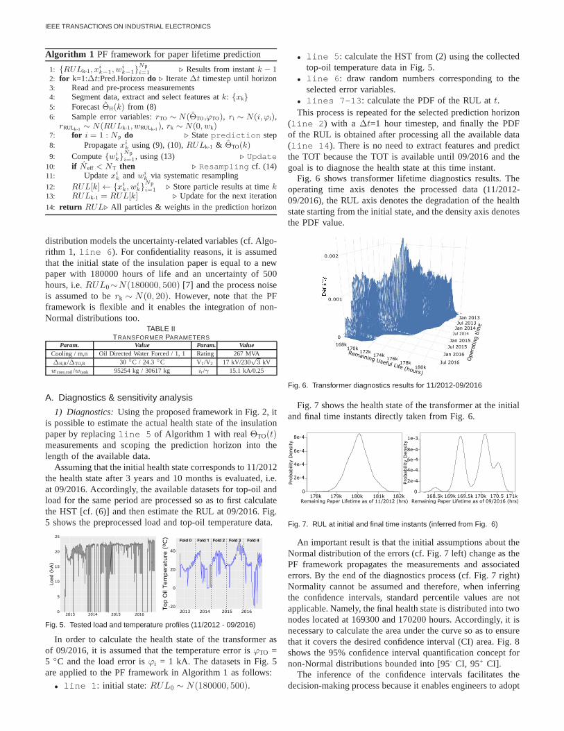
• line 5: calculate the HST from (2) using the collectedtop-oil temperature data in Fig. 5.

• line 6: draw random numbers corresponding to theselected error variables.

• lines 7-13: calculate the PDF of the RUL att.This process is repeated for the selected prediction horizon

(line 2) with a ∆t=1 hour timestep, and finally the PDFof the RUL is obtained after processing all the available data(line 14). There is no need to extract features and predictthe TOT because the TOT is available until 09/2016 and thegoal is to diagnose the health state at this time instant.

Fig. 6 shows transformer lifetime diagnostics results. Theoperating time axis denotes the processed data (11/2012-09/2016), the RUL axis denotes the degradation of the healthstate starting from the initial state, and the density axis denotesthe PDF value.

0.002

0.001

0

D��

Jul 2016

Jan 2016

Jan 2015

Jan 2014Jul 2013

Jul 2014

Jul 2015

180k

176k174k

172k170k

168k

178k

Remaining Useful Life (hours)

Opera

ting t

ime

Jan 2013

Fig. 6. Transformer diagnostics results for 11/2012-09/2016

Fig. 7 shows the health state of the transformer at the initialand final time instants directly taken from Fig. 6.

Fig. 7. RUL at initial and final time instants (inferred from Fig. 6)

An important result is that the initial assumptions about theNormal distribution of the errors (cf. Fig. 7 left) change asthePF framework propagates the measurements and associatederrors. By the end of the diagnostics process (cf. Fig. 7 right)Normality cannot be assumed and therefore, when inferringthe confidence intervals, standard percentile values are notapplicable. Namely, the final health state is distributed into twonodes located at 169300 and 170200 hours. Accordingly, it isnecessary to calculate the area under the curve so as to ensurethat it covers the desired confidence interval (CI) area. Fig. 8shows the 95% confidence interval quantification concept fornon-Normal distributions bounded into [95- CI, 95+ CI].

The inference of the confidence intervals facilitates thedecision-making process because it enables engineers to adopt


Fig. 8. 95% confidence intervals [95- CI, 95+ CI]

an uncertainty-informed decision with intuitive lower andupper limits on the estimated parameters. Accordingly, Fig. 9shows the maximum likelihood and 95% CI of the predictionsin Fig. 6.

Fig. 9. Transformer diagnostics, 95% CI of Fig. 6

Fig. 9 shows the maximum likelihood and 95% CI for thePDFs shown in Fig. 6. The degradation is almost exponentialas determined by the ageing acceleration factor in (1), butthis is affected by the de-energized periods of the transformerwhich are reflected in the load and top-oil temperature. Forexample, the transformer was shut down in mid-2016 whichresulted in zero load, decreased top-oil temperature, andaccordingly almost negligible RUL decrease. The uncertaintypropagation is dependent on the assumed error variables andprocessed data as discussed in the next subsection.

2) Sensitivity Analysis:In order to evaluate the effect oferror variables on the RUL estimation a sensitivity analysis hasbeen performed examining the effect of the change of load andtemperature measurement errors. Note that this information islost with existing lifetime estimation models.

The HST in (6) defines the effect of load and temperaturemeasurements errors. For this case study (cf. Table II), thisequation is parametrized as follows (i(t), ϕi are in kA units):

ΘH(t) =ΘTO(t)+ϕTO+ [∆H,R/ir2].[i(t)2+ϕi

2+2.i(t).ϕi ]

=ΘTO(t)+ϕTO+0.13.i(t)2+0.13.ϕi2+0.13.i(t).ϕi

(15)

It is possible to see that the effect of temperature measure-ment errors are added as absolute values. In contrast, for smallload variations, the effect of load measurement errors on theHST are not relevant. However, ifϕi >

√

(1/0.13) ∼2.78 thenthe effect starts increasing rapidly due to the factor0.13.ϕi

2

and the exponential degradation in (7). The term0.13.i(t).ϕi

depends on the specific transformer loading.The effects of different load and temperature errors have

been analysed using monitored data. For computational effi-ciency the data has been limited to a year (11/2012-11/2013).Fig. 10 shows the effect of different load measurement errorson lifetime estimation assuming constant temperature mea-surement error (N(ΘTO, 5)) and process noise (N(0, 20)).

110k120k

110k130k140k

150k160k

1��k1��k

5

4

3

2

1

0

Load e

rror

(kA)

R�� ng Useful Life (hours)

0

0�00�

0�00�

0�00�

��

Fig. 10. Load error sensitivity analysis — 3D representation

It is apparent from Fig. 10 that different load measurementerrors play a different role on the lifetime estimation. Fig. 11shows the maximum likelihood and 95% CI for the load errorsensitivity analysis inferred from Fig. 10.

Load error (kA)

RU

L (

hours

)

180k

9� � �o�� !"#$l

160k

140k

120k

0 1 2 3 4 5

17

17

18

2�%&

Fig. 11. Load error sensitivity analysis with 95% CIs

As the load measurement error magnitude increases inFig. 11, the uncertainty bounds increase and the maximumlikelihood value decreases. The zoomed view of the interval[0.01-1] kA shows that the error bounds are around 2000 hoursand they are fairly constant in this zone. However, around theelbow point identified in (15) the maximum likelihood valuestarts decreasing rapidly and the 95% confidence intervalswiden due to the increased effect of the error values. Owingto the stochastic nature of the PF algorithm, the 95% CIs varyaccording to the nature of the PDF (see PDFs in Fig. 10).

In order to evaluate the effect of temperature errors, the loadmeasurement error (N(i(t), 1)) and process noise (N(0, 20))have been assumed constants. Fig. 12 shows the 95% CI foreffect of error measurements for this situation.

In Fig. 12 one can see that for temperature measurementerror values below 5◦C, the effect of temperature measurementerrors on the RUL estimation is unstable. That is, the maxi-mum likelihood value of the PDF of the RUL value fluctuatesaroundRUL0=N(180000, 500) minus the ageing after oneyear. Depending on the initial state which is randomly sampledfrom RUL0, the final health state varies. There are some caseswhere the initial RUL is located around 180500 hours andtherefore, after a year with a degradation lower than 500 hours,the final health state is above 180000 hours.


Fig. 12. Temperature error sensitivity analysis

On the other hand, above a temperature error of 5◦C theeffect of the temperature error becomes non-negligible anditdirectly affects the health state. Additionally, it is possible tosee that for temperature measurement error values below 2◦Cthe CIs are very narrow, but as the error increases these boundswiden. This is because for low temperature errors the model isconfident that the final health state is the maximum likelihoodvalue because there is no temperature error. However, asthe temperature error increases, the CIs widen and the finalevaluation of the health state is more uncertain.

When the load error is zero and the temperature measure-ment error is 5◦C (Fig. 11) the variation of the RUL estimationis caused by the termϕTO in (15). In contrast, when thetemperature measurement error is zero in Fig 12, but the loaderror is kept at 1kA, it can be seen that the variation due tothe termϕi in (15) is almost negligible, which confirms thatthe effect of temperature errors are more sensitive than loaderrors for low loading conditions.

B. PrognosticsIn order to predict the future health state of the transformer

the approach shown in Fig. 2 is adopted. First an appropriatepredictive model is designed which is able to estimate HSTgiven hypothetical load and temperature profiles. This estima-tion can then be directly connected with the PF framework topropagate uncertainties and estimate the lifetime. The adoptedtemperature error isϕTO = 5◦C and load errorϕi = 1 kA.

1) Feature processing & selection:The length of thesegment determines the validity of features and the finalprediction error. According to the performed experiments,bestresults were obtained with a length of 5 days. With a segmentlength longer than this the features lost representativeness andthe error increases (see Fig. 13) .

Subsequently, all the features (cf. Table I) along withthe preprocessed variables have been processed through arecursive feature elimination (RFE) procedure and grid search[35]. This step selects the most representative features whichminimize the prediction error. RFE was implemented for RF,XGB and SVR using theCaret R package and grid searchwas implemented for ANN and LSTM models. The error isquantified through 10 repeated 5 fold CV using the normalisedroot-mean-squared error (RMSE):

RMSE=RMSE

max{RMSE i}Ni=1

;RMSE=

√

√

√

√

∑

Ni=1

(

ΘTO − ΘTO

)2

N(16)

whereN is the number of predicted data samples.Fig. 13 shows the feature selection results with best features

for different segment sizes for XGB and RF models. Bestresults were obtained with the listed 12 features in Fig. 13.

Fig. 13. Feature selection and segment size

Best results for SVR were obtained with three features(water temperature, mean ambient temperature, load), nineforANN models (water temperature, mean ambient temperature,mean load, RMS water temperature, mean water temperature,skewness water temperature, RMS load, kurtosis ambient tem-perature, IF ambient temperature) and six for LSTM models(water temperature, mean ambient temperature, load, RMSload, mean load, mean water temperature) all with a segmentsize of 5 days. After the feature extraction step, all theforecasting models have been designed and trained accordingto the process outlined in Subsections III-B1-III-B5.

2) Thermal modelling:The first step is to learn a predictivemodel so as to predict the top-oil temperature. Figs. 5 and 14show load, ambient, water and top-oil measurements hourlysampled for a period of 3 years and 10 months.

Fig. 14. Water and ambient temperature data (11/2012-09/2016)

It can be seen that the top-oil temperature profile is highlynon-linear due to the specific operational constraints of NPPs.Namely, the plant is shut down for maintenance activitiesand this affects the load and top-oil temperature values.Additionally, depending on the harshness of the winter, loadconditions and applied water temperature, the oil temperaturecan drop below zero degrees, e.g. winter 2016.

The learning process includes a 10 repeated 5 fold CVprocedure to estimate parameters and generalize the predictionresults. That is, the top-oil time series is divided into 5equidistant folds (see Fig. 5). Then a number of ML modelsare trained (see Subsection III-B) for the first fold and testedwith the second fold, subsequently the same models are trainedwith the first two folds and then tested with the third fold andthe validation continues until the last step, where the modelsare trained with the first four folds and tested on the last fold.This process is repeated 10 times to deal with the stochastic


behaviour of some models and generate repeatable results. Forthe error calculation the RMSE has been used. Note that thereare different alternatives to validate the results such as thestratified double CV scheme [26].

In total, after preprocessing the data and removing invalidsamples, there are 32440 samples so each fold has 6488samples. Accordingly, at each fold the models predict up to6488 hours ahead (∼ 271 days). Table III displays the meanRMSE and the standard deviation for various models for all thefolds estimated through the 10 repeated 5 fold CV procedure.

TABLE IIIRMSE OF ML MODELS FOR TOP-OIL TEMPERATURE FORECASTING

Tech.Fold #1 Fold #2 Fold #3 Fold #4 Average

etrain etest etrain etest etrain etest etrain etest etrain etest

XGB0.37±0.28

4.13±0.37

1.2±0.35

5.07±0.35

2.08±0.13

6.63±0.67

3.04±0.24

9.1±0.15

1.67±1.14

6.23±

2.17

LSTM(2L)

1.77±0.05

3.99±

0.42

2.45±0.12

4.13±0.3

2.89±0.15

6.85±0.25

4.63±0.28

9.97±0.39

2.94±1.05

6.24±2.43

LSTM(3L)

1.82±0.09

4.31±029

2.43±0.33

4.39±0.24

3.01±0.28

6.67±0.24

4.21±0.6

9.7±0.11

2.87±0.88

6.27±2.19

LSTM(1L)

2±0.17

4.3±0.71

2.52±0.24

4.4±0.49

3.29±0.52

6.9±0.26

4.34±0.67

9.6±0.52

3.05±1.01

6.3±2.5

RF0.85±0.02

4.23±0.05

0.84±0.01

5.05±0.06

0.91±0.005

6.49±0.001

1.07±0.005

10±0.005

0.92±0.1

6.4±2.55

SVR 1.66 4.9 2.87 4.13 2.38 6.93 3.5 9.762.35±0.77

6.43±2.51

ANN1.12±1.04

5.8±1.6

1.49±0.27

5.47±0.83

2.07±0.14

6.54±0.18

3.43±0.19

11.07±0.93

2.03±1.01

7.22±2.6

IEEEC57.91

N/A 5 N/A 5.6 N/A 8.6 N/A 12 N/A7.77±3.2

From the prediction results in Table III it can be seenthat the XGB predicts best the top-oil temperature value. Themean performance of the LSTM is practically the same, butin the worst case scenario the maximum error is greater thanthe XGB, i.e.etestXGB = 8.4< etestLSTM=8.67. Additionally, animportant advantage of XGB over LSTM is that XGB modelsare easier and faster to train and test. Accordingly, the XGBmodel is used for lifetime modelling and RUL estimation. Fig.15 shows the last fold prediction for XGB and LSTM, whereground truth denotes the measured top-oil temperature data.

Fig. 15. Top-oil temperature forecasting results for the last fold (seetop-oil temperature and folds in Fig. 5)

RF also shows a good performance, but the problem is thatRF overfits the model as shown by the low training error. Alsonote that different trials of SVR models generate same resultsbecause of the fixed decision boundaries.

In contrast, the thermal model defined in the IEEE C57.91standard has the poorest performance and highlights that the

IEEE analytic model may not perform accurately for everytransformer operating in different contexts.

3) Lifetime modelling:The lifetime prediction model usesthe most accurate thermal model within the framework in Fig.2. Given hypothetical ambient temperature, load and watertemperature variables, first the selected features are inferred(cf. Fig. 13), and then the XGB model predicts the top-oil temperature. Subsequently, the IEEE model is used toestimate the hot-spot temperature from the predicted top-oiltemperature, and finally, this is used to predict the paper RULusing the PF framework defined in Algorithm 1.

To test the approach with different hypothetical profiles, oneyear’s worth top-oil and ambient temperature data have beentaken from Fig. 14 as a representative reference for yearlytemperature patterns. Then user-defined load profiles are usedto predict the TOT under different loading conditions. Fig.16shows tested load and temperature patterns.

Fig. 16. Tested future load and temperature profiles

These patterns have been repeatedly applied to the PFframework in Algorithm 1 for two different prediction hori-zons of 5 and 10 years:

• line 1: initial state:RUL0 ∼ N(180000, 500).• line 4: infer selected features from load, ambient tem-

perature and water temperature profiles in Fig. 16.• line 5: using the designed XGB model, first forecast

the TOT and then calculate the HST.• line 6: draw random numbers corresponding to the

assumed error variables.• lines 7-13: calculate the PDF of the RUL at time

instantt.

This process is repeated for the selected prediction horizon(line 2) with a ∆t=1 hour timestep, and finally the PDFof the RUL is obtained after processing the data up untilthe prediction horizon (line 14). Fig. 17 shows the RULpredictions after 5 and 10 years.

Fig. 17. Predicted RUL with the scenarios in Fig. 16

The initial state statistics in Fig. 17 are mean=179800,95+=180900, 95-=178900 (all in hours). Table IV displaysRUL statistics corresponding to different profiles.


TABLE IVRUL STATISTICS IN F IG. 17

TimeProfile A Profile B Profile C

m 95+ 95- m 95+ 95- m 95+ 95-

5y 178.9k 180.1k 178.6k 177.6k 178.1k 176.5k 169.9k 170.4k 168.4k10y 178.5k 179.1k 177.1k 174.2k 174.3k 173.7k 158.9k 159.8k 158.4k

The predicted RUL values are consistent with the appliedprofiles. That is, C shows the most severe degradation followedby B, and the application of A results in a higher RUL.

V. CONCLUSIONS

This paper has presented a novel transformer conditionassessment approach integrating model-based experimentalmodels, forecasting models and uncertainty modelling con-cepts in a Bayesian Particle Filtering framework.

Error propagation and sensitivity analysis are key activitiesfor decision-making under uncertainty. The implemented sen-sitivity analysis evaluated the effect of load and temperaturemeasurement errors on transformer lifetime and it showed thatfor low load measurement errors the effect of temperatureerrors are more critical. However, the load measurementerror increases rapidly above an elbow value which has beenformulated analytically.

It has been demonstrated that the integration of machinelearning (ML) models with experimental models improvestransformer lifetime estimations. Among the tested ML modelsfor thermal modelling, the eXtreme Gradient Boosting (XGB)has shown the best prediction performance. Accordingly, thetransformer RUL has been examined with different operationalprofiles using the XGB-based temperature prediction model,IEEE-based lifetime model and uncertainty information of col-lected measurements and stochastic processes. The predictedRUL values are consistent with the applied operational profilesand this demonstrates the validity of the proposed approachfor adaptive lifetime predictions.

As NPPs age, the aging of transformers is becoming increas-ingly critical because they are crucial assets to export energyfrom the NPP. The proposed approach enables the modellingof these dynamic contexts accurately while accounting foruncertainties. Future work may focus on integrating otherdegradation accelerating factors in the proposed approachsuchas the moisture and other chemical factors.

REFERENCES

[1] W. H. Tang and Q. Wu,Condition monitoring and assessment of powertransformers using computational intelligence. Springer, London, 2011.

[2] M. Liserre, G. Buticchi, M. Andresen, G. Carne, L. Costa,and Z. Zou,“The smart transformer: Impact on the electric grid and technologychallenges,”IEEE Ind. Electron. Mag., vol. 10, no. 2, pp. 46–58, 2016.

[3] H. Ma, T. K. Saha, C. Ekanayake, and D. Martin, “Smart transformer forsmart grid - intelligent framework and techniques for powertransformerasset management,”IEEE Trans. Smart Grid, vol. 6, no. 2, pp. 1026–1034, 2015.

[4] J. Aizpurua, V. Catterson, B. Stewart, S. McArthur, B. Lambert, B. Am-pofo, G. Pereira, and J. Cross, “Determining appropriate data analyticsfor transformer health monitoring,” inNPIC-HMIT, pp. 1–11, 4 2017.

[5] M. Djamali and S. Tenbohlen, “Hundred years of experience in thedynamic thermal modelling of power transformers,”IET Generation,Transmission Distribution, vol. 11, no. 11, pp. 2731–2739, 2017.

[6] A. Teymouri and B. Vahidi, “Co2/co concentration ratio:A comple-mentary method for determining the degree of polymerization of powertransformer paper insulation,”IEEE Elect. Insul. Mag., vol. 33, no. 1,pp. 24–30, 2017.

[7] IEEE PES, “IEEE Guide for Loading Mineral-Oil-ImmersedTransform-ers and Step-Voltage Regulators,”IEEE Std. C57.91, 2011.

[8] R. Medina, A. Romero, E. Mombello, and G. Ratta, “Assessing degra-dation of power transformer solid insulation considering thermal stressand moisture variation,”Electr. Pow. Syst. Res., vol. 151, pp. 1–11, 2017.

[9] Y. Cui, H. Ma, T. Saha, C. Ekanayake, and D. Martin, “Moisture-dependent thermal modelling of power transformer,”IEEE Trans. Pow.Del., vol. 31, no. 5, pp. 2140–2150, 2016.

[10] A. Seier, P. D. H. Hines, and J. Frolik, “Data-driven thermal modeling ofresidential service transformers,”IEEE Trans. Smart Grid, vol. 6, no. 2,pp. 1019–1025, 2015.

[11] E. Pournaras and J. Espejo-Uribe, “Self-repairable smart grids via onlinecoordination of smart transformers,”IEEE Trans. Ind. Infor., vol. 13,no. 4, pp. 1783–1793, 2017.

[12] M. Andresen, V. Raveendran, G. Buticchi, and M. Liserre, “Lifetime-based power routing in parallel converters for smart transformer appli-cation,” IEEE Trans. Ind. Electron., vol. 65, no. 2, pp. 1675–1684, 2018.

[13] J. Velasquez, M. Sanz, and S. Galceran, “General asset managementmodel in the context of an electric utility: application to power trans-formers,” Electr. Pow. Syst. Res., vol. 81, no. 11, pp. 2015–2037, 2011.

[14] D. Villacci, G. Bontempi, A. Vaccaro, and M. Birattari,“The roleof learning methods in the dynamic assessment of power componentsloading capability,”IEEE Trans. Ind. Electron., vol. 52, no. 1, pp. 280–290, Feb. 2005.

[15] M. Hell and P. Costa and F. Gomide, “Participatory learning in powertransformers thermal modeling,”IEEE Trans. Pow. Del., vol. 23, no. 4,pp. 2058–2067, Oct. 2008.

[16] L. Souza, A. Lemos, W. Caminhas, and W. Boaventura, “Thermal mod-eling of power transformers using evolving fuzzy systems,”EngineeringApplications of Artificial Intelligence, vol. 25, no. 5, pp. 980 – 988, 2012.

[17] A. Bracale, G. Carpinelli, M. Pagano, and P. D. Falco, “Aprobabilisticapproach for forecasting the allowable current of oil-immersed trans-formers,” IEEE Trans. Pow. Del., vol. PP, no. 99, pp. 1–1, 2018.

[18] Q. Chen and D. M. Egan, “A bayesian method for transformer lifeestimation using perks’ hazard function,”IEEE Trans. Pow. Sys., vol. 21,no. 4, pp. 1954–1965, 2006.

[19] D. Zhou, Z. Wang, and C. Li, “Data requisites for transformer statisticallifetime modelling - part I: Aging-related failures,”IEEE Trans. Pow.Del., vol. 28, no. 3, pp. 1750–1757, 2013.

[20] E. Chiodo, D. Lauria, F. Mottola, and C. Pisani, “Lifetime characteri-zation via lognormal distribution of transformers in smartgrids: Designoptimization,” Applied Energy, vol. 177, pp. 127 – 135, 2016.

[21] M. Humayun, M. Z. Degefa, A. Safdarian, and M. Lehtonen,“Utilizationimprovement of transformers using demand response,”IEEE Trans. Pow.Del., vol. 30, no. 1, pp. 202–210, 2015.

[22] V. M. Catterson, J. Melone, and M. S. Garcia, “Prognostics of trans-former paper insulation using statistical particle filtering of on-line data,”IEEE Elect. Insul. Mag., vol. 32, no. 1, pp. 28–33, Jan. 2016.

[23] L. Jauregui-Rivera, X. Mao, and D. Tylavsky, “Improving reliabilityassessment of transformer thermal top-oil model parameters estimatedfrom measured data,”IEEE Trans. Pow. Del., vol. 24, no. 1, pp. 169–176,2009.

[24] W. H. Tang, K. Spurgeon, Q. H. Wu, and Z. J. Richardson, “An evidentialreasoning approach to transformer condition assessments,” IEEE Trans.Pow. Del., vol. 19, no. 4, pp. 1696–1703, 2004.

[25] T. W. Rauber, F. Boldt, and F. M. V. ao, “Heterogeneous feature modelsand feature selection applied to bearing fault diagnosis,”IEEE Trans.Ind. Electron., vol. 62, no. 1, pp. 637–646, Jan. 2015.

[26] R. Razavi-Far, M. Farajzadeh-Zanjani, and M. Saif, “Anintegrated class-imbalanced learning scheme for diagnosing bearing defectsin inductionmotors,” IEEE Trans. Ind. Infor., vol. 13, no. 6, pp. 2758–2769, 2017.

[27] L. Breiman, “Random forests,”Machine Learning, vol. 45, no. 1, pp.5–32, Oct. 2001.

[28] M. R. G. Meireles, P. E. M. Almeida, and M. G. Simoes, “A compre-hensive review for industrial applicability of artificial neural networks,”IEEE Trans. Ind. Electron., vol. 50, no. 3, pp. 585–601, Jun. 2003.

[29] A. J. Smola and B. Scholkopf, “A tutorial on support vector regression,”Statistics and Computing, vol. 14, no. 3, pp. 199–222, Aug. 2004.

[30] T. Chen and C. Guestrin, “Xgboost: A scalable tree boosting system,” inProc. of ACM Knowledge Discov. & Data Mining, pp. 785–794, 2016.

[31] S. Hochreiter and J. Schmidhuber, “Long short-term memory,” NeuralComputation, vol. 9, no. 8, pp. 1735–1780, 1997.

[32] J. Friedman, T. Hastie, and R. Tibshirani, “Additive logistic regression:a statistical view of boosting,”Ann. Statist., vol. 28, no. 2, pp. 337–407,2000.


[33] M. S. Arulampalam, S. Maskell, N. Gordon, and T. Clapp, “A tutorialon particle filters for online nonlinear/non-gaussian bayesian tracking,”IEEE Trans. Signal Process., vol. 50, no. 2, pp. 174–188, Feb. 2002.

[34] B. Saha and K. Goebel, “Model adaptation for prognostics in a particlefiltering framework,” Int. J. of Prognostics and Health Management,vol. 2, no. 6, 2011.

[35] M. Kuhn and K. Johnson,An Introduction to Feature Selection, pp.487–519. New York, NY: Springer New York, 2013.

Jose Ignacio Aizpurua (M’17) is a ResearchAssociate within the Institute for Energy and En-vironment at the University of Strathclyde, Scot-land, UK. He received his Eng., M.Sc., and Ph.D.degrees from Mondragon University (Spain) in2010, 2012, and 2015 respectively. He was avisiting researcher in the Dependable SystemsResearch group at the University of Hull (UK) in2014. His research interests include prognosticsand health management, reliability, availability,maintenance and safety (RAMS) analysis and

systems engineering for power engineering applications.

Victoria M. Catterson (M’06-SM’12) is a SeniorLecturer within the Institute for Energy and En-vironment at the University of Strathclyde, Scot-land, UK. She received her B.Eng. (Hons) andPh.D. degrees from the University of Strathclydein 2003 and 2007 respectively. Her researchinterests include condition monitoring, diagnos-tics, and prognostics for power engineering ap-plications

Brian G. Stewart (M’08) is is Professor withinthe Institute of Energy and Environment at theUniversity of Strathclyde, Glasgow, Scotland. Hegraduated with a BSc (Hons) and PhD from theUniversity of Glasgow in 1981 and 1985 respec-tively. He also graduated with a BD (Hons) in1994 from the University of Aberdeen, Scotland.His research interests are focused on high volt-age engineering, electrical condition monitoring,insulation diagnostics and communication sys-tems. He is currently an AdCom Member within

the IEEE Dielectrics and Electrical Insulation Society.

Stephen D. J. McArthur (M’93-SM’07-F’15) re-ceived the B.Eng. (Hons.) and Ph.D. degreesfrom the University of Strathclyde, Glasgow,U.K., in 1992 and 1996, respectively. He is aProfessor and co-Director of the Institute forEnergy and Environment at the University ofStrathclyde. His research interests include intel-ligent system applications in power engineering,covering condition monitoring, diagnostics andprognostics, active network management andwider smart grid applications.

Brandon Lambert is a Design EngineeringManager within Bruce Power. He received hisB.Eng. degree from Lakehead University, Thun-der Bay, Canada in 2012 and his P.Eng. from theProfessional Engineers of Ontario in 2015. Hisdesign interests include large power transform-ers, high voltage transmission systems, as wellas dielectric and insulating materials.

James Cross (M ’79) is currently Directorof Transformer Services at Kinectrics, In. inToronto, Canada. After graduating from the Uni-versity of Manitoba with a B.Sc. in Electri-cal Engineering, he worked for 18 years atCarte International, a transformer manufacturerin Winnipeg, Canada as Vice-President, Tech-nology. He then worked as a Project Engineerat Pauwels Canada, a manufacturer of largepower transformers up to 500 kV class. Mostrecently, he worked for 18 years at Weidmann

Electrical Technology in St. Johnsbury, Vermont serving as Managerof R&D/Innovation and Manager of Technical Services. He has co-authored several papers in the area of electrical insulating materials andtesting, and transformer diagnostics. He is a former Chairperson of theIEEE Winnipeg Section.

adaptive power transformer lifetime predictions through ... · transformer loading capability and...

Documents