adaptive nulling with weight constraints … in electromagnetics research b, vol. 26, 23{38, 2010...

Progress In Electromagnetics Research B, Vol. 26, 23–38, 2010

ADAPTIVE NULLING WITH WEIGHT CONSTRAINTS

R. L. Haupt

Applied Research LaboratoryPennsylvania State UniversityP. O. Box 30, State College, PA 16803, USA

Abstract—Adaptive nulling algorithms that minimize the total arrayoutput power from the array require constraints on the adaptiveweights, otherwise nulls would be placed in the main beam andthe desired signal rejected. The concept of cancellation patternsis reviewed and extended to partial adaptive nulling. Cancellationpatterns are then extracted from adaptive nulling results with a geneticalgorithm and a 32 element dipole array model. The cancellationpatterns provide insight into the constraints needed for the successfulimplementation of a power minimization adaptive algorithm.

1. INTRODUCTION

An adaptive array manipulates the antenna pattern using amplitudeand phase weighting of the element signals in order to receive thedesired signal entering the main beam while placing nulls in thedirections of the interfering signals entering the sidelobes. Mostadaptive nulling algorithms require an estimate of the signal correlationmatrix in order to find the adapted weights [1]. These algorithmsare based upon the Wiener Hopf solution and find the adaptiveweights by optimizing a performance measure like signal to noise ratio.Eigenvectors and eigenvalues of the autocorrelation matrix indicate thenumber, locations, and strengths of the signals incident on the array [2].

The problem with most adaptive algorithms is that they need toaccurately know the signal at each element in the array in order to formthe estimate of the signal correlation matrix [3]. Errors in the signalpath cause corresponding errors in the correlation matrix that resultin adaptive weights that do not place the desired nulls in the sidelobes.Consequently, extensive array calibration and compensation schemes

Received 8 July 2010, Accepted 10 September 2010, Scheduled 23 September 2010Corresponding author: R. L. Haupt ([email protected]).

24 Haupt

are required in order to equalize path lengths and signal strengths atthe elements [4].

Digital beamforming offers the best approach to hosting anadaptive nulling algorithm, because all of the weight adjustmentsare done in software [5]. Although digital beamforming is becomingmore widely available [6], most antenna arrays deliver signals to andreceive signals from the elements via a corporate feed. T/R modulesplaced at each element form an active electronically scanned array thatelectronically steers beams [7]. The T/R modules provide control overthe amplitude and phase of the signals at the elements but do notdetect the signals at each element. A passive electronically scannedarray has phase shifters at each element and little to no amplitudecontrol.

Another approach to adaptive nulling minimizes the total outputpower of the array [8]. Since setting the amplitudes at eachelement equal to zero minimizes the output power, amplitude weightconstraints are necessary for a practical adaptive antenna system.An alternative to nulling with amplitude weights that preserves thequiescent amplitude taper is phase-only nulling [9]. Even thoughphase-only nulling cannot zero the amplitude weights, it can set halfthe elements out of phase with the other half in order to form a null inthe middle of the main beam and reject the desired signal. Limiting thephase by using only the least significant bits in the phase shifters hasbeen suggested as a solution to this problem [10]. Another approach,called partial adaptive nulling, limits the nulling of the desired signalby making only a subset of the elements in the array adaptive [11].This approach limits the damage to the main beam while allowingnulls to be placed in the sidelobes.

Placing a null in an array pattern is equivalent to subtracting acancellation pattern from the quiescent pattern when the cancellationpattern equals the quiescent pattern at the desired null locations.There are an infinite number of cancellation patterns that can placethe null(s). Section 2 presents mathematical representations for thecancellation beam. Section 3 presents techniques for synthesizingpatterns with desired nulls (deterministic nulling). Section 4 presentsadaptive nulling results for a model that used a genetic algorithm anda full wave electromagnetic model of a 32 element dipole array. Thegenetic algorithm minimizes the total output power by employing theweight constraints introduced in Section 3. The cancelation patternfor the adaptive nulling results are found by subtracting the quiescentpattern from the adapted pattern. A similar approach is used inSection 5 to find the cancelation pattern for experimental adaptedpatterns.

Progress In Electromagnetics Research B, Vol. 26, 2010 25

2. CANCELLATION PATTERNS

This section establishes the definitions of the quiescent, adapted, andcancellation patterns that are used in this paper. The quiescent patternof an N -element linear array along the x-axis is defined by its amplitudetaper (an) and the main beam steered to φ = 90◦ as measured fromthe positive x-axis.

QP =N∑

n=1

anejk(n−1)d cos φ (1)

where d is the element spacing and k is the wavenumber. An adaptivearray modifies the amplitude and/or phase of the element weights inorder to place M nulls in the directions of interference, φm. The nulledarray factor can be written as [12]

AF =N∑

n=1

wnejk(n−1)d cos φ

=N∑

n=1

anejk(n−1)d cos φ −M∑

m=1

γm

N∑

n=1

anejk(n−1)d(cos φ−cos φm)

= QP + CP (2)

whereγm = sidelobe level of the quiescent pattern at φm.

wn = an −M∑

m=1γmcne−jnkd cos φm = adapted weights.

cn = amplitude taper of the cancellation beam.When cn = an, the cancelation pattern is identical to the quiescent

pattern. When cn = 1.0, the cancelation pattern is a uniform arrayfactor. For instance, if the array is uniform (an = 1), then

γm =sin (Nkd cosφm/2)N sin (kd cosφm/2)

(3)

The adaptive weights can also be written as perturbations to thequiescent weights.

wn = an (1−∆n) ejδn 0 ≤ ∆n ≤ 1 and 0 ≤ δn ≤ 2π (4)

where ∆n and δn are the amplitude and phase perturbations from thequiescent weights, respectively. Substituting (4) into (2) and solving

26 Haupt

for the cancellation pattern yields

CP = AF −QP

=N∑

n=1

(1−∆n) ejδnanejk(n−1)d cos φ −N∑

n=1

anejk(n−1)d cos φ

=N∑

n=1

(ejδn −∆nejδn − 1

)anejk(n−1)d cos φ (5)

Thus, the cancellation pattern for any computed or measured adaptedpattern is found by simply subtracting the quiescent pattern from theadapted pattern.

If the amplitude and phase of the adapted weights are small(such as when constraints are placed on the adaptive weights), thenejδn ≈ 1 + jδn for δn ¿ 1, and the cancellation pattern is given by

CP ≈N∑

n=1

[1 + jδn −∆n (1 + jδn)− 1] anejk(n−1)d cos φ

≈N∑

n=1

(jδn −∆n) anejk(n−1)d cos φ (6)

Phase-only nulling (∆n = 0) has a cancelation pattern given by

CP ≈N∑

n=1

jδnanejk(n−1)d cos φ (7)

3. NULL SYNTHESIS AND CANCELATION PATTERNS

Null synthesis is an open loop process that derives weights that placenulls in the array factor at known locations. Setting the array factorin (2) equal to zero at M different angles (the size of M depends uponthe number of adjustable or adaptive weights)

N∑

n=1

an (1−∆n) ejδnejk(n−1)d cos φm = 0, m = 1, 2, . . . , M (8)

Writing (8) in matrix form results in

Ax = b (9)


where

A =

a1 · · · aNejk(N−1)d cos φ1

.... . .

...a1 · · · aNejk(N−1)d cos φM

x =[(1−∆1) ejδ1 · · · (1−∆N ) ejδN

]T

b = [0 · · · 0]T

The phase term in x requires a nonlinear solution to this equation.For low sidelobes, only small perturbations to the weights are

needed to place nulls. Assuming that ∆n ¿ 1 and δn ¿ 1results inlinearizing (9) with

x = [∆1 − jδ1 · · · ∆N − jδN ]T

b =[

N∑n=1

anejk(n−1)d cos φ1 · · ·N∑

n=1anejk(n−1)d cos φM

]T

Now, a linear matrix solver finds the weight perturbations needed toplace the nulls.

An adaptive array that has Na(Na < N) variable weights forplacing nulls is known as a partially adaptive array. The weights in (4)for a partially adaptive array are given by

wn ={

an (1−∆n) ejδn if element n is adaptivean if element n is not adaptive (10)

The first examples demonstrating null synthesis assume a fullyadaptive array, Na = N . Consider a linear array of 32 isotropic pointsources spaced λ/2 apart. The quiescent array has a 30 dB n̄ = 7Taylor taper. Fig. 1 overlays the quiescent pattern, adapted pattern,and cancelation pattern when a null is synthesized at φ = 106.25◦.When cn = 1, the patterns in Fig. 1(a) result. The adapted patternis minimally perturbed near the null, because the beamwidth of thecancelation beam is a minimum. When cn = an, the patterns inFig. 1(b) result. The sidelobes near the synthesized null in theadapted pattern become over 2 dB higher, because the beamwidth ofthe cancelation beam is wider due to the amplitude taper.

A second example places the same null in the array factor usingphase-only nulling with cn = an. The cancelation pattern is shownsuperimposed on the quiescent and adapted patterns in Fig. 2. Notethe increased sidelobe in the symmetric location about the main beam(φ = 73.75◦). These symmetric sidelobes can only be eliminated usingvery large phase shifts [13] which cause severe array factor distortions.

28 Haupt

(a) (b)

Figure 1. Null placed at φ = 106.25◦ in 30 dB n̄ = 7 Taylor quiescentpattern with cancelation patterns that are (a) uniform cn = 1.0 (b)tapered cn = an.

Figure 2. The cancelation pattern (dashed line) superimposed onthe quiescent pattern and adapted pattern when a null is placed atφ = 106.25◦ using phase weights and cn = an.

Figure 3 shows the cancelation patterns associated with placinga null at φ = 106.25◦ in the array factor when Na = 8 out of theN = 32 elements have adaptive weights. Four different partiallyadaptive array configurations are considered that have the followingadaptive elements:

(a) 1, 2, 3, 4, 29, 30, 31, 32;(b) 13, 14, 15, 16, 17, 18, 19, 20;(c) 1, 5, 9, 13, 17, 21, 25, 29;(d) 2, 8, 13, 16, 18, 23, 24, 30.


(c) (d)

(a) (b)

Figure 3. Cancelation patterns for 4 different selections of adaptiveelements that place a null at φ = 106.25◦. The array at the top of theplots shows a diagram of the linear array along the x-axis. Adaptiveelements are indicated by large squares. (a) adaptive elements: 1, 2, 3,4, 29, 30, 31, 32; (b) adaptive elements: 13, 14, 15, 16, 17, 18, 19, 20;(c) adaptive elements: 1, 5, 9, 13, 17, 21, 25, 29; (d) adaptive elements:2, 8, 13, 16, 18, 23, 24, 30.

All the configurations have a cancelation pattern peak at φ =106.25◦, but the rest of the cancelation patterns are very different.

The location of the adaptive elements determines the shape ofthe cancelation pattern which in turn determines the distortion tothe adapted pattern. When 4 elements on each end of the array areadaptive, then a very broad but highly oscillatory cancelation patternmain beam results as shown in Fig. 3(a). When 8 adaptive elementsare contiguous, then the cancelation beam in Fig. 3(b) results. Thiscancelation pattern is just an 8 element uniform array factor with itsmain beam steered to φ = 106.25◦. Separating the adaptive elements

30 Haupt

by regular intervals induces grating lobes in the cancelation patternas shown in Fig. 3(c). Random spacing of the adaptive elementsproduces the high sidelobe but narrow main beam cancelation patternin Fig. 3(d).

4. ADAPTIVE NULLING WITH WEIGHTCONSTRAINTS

Partial adaptive nulling is one way to prevent unwanted main beamnulling when minimizing the total output power. Another way is toput upper bounds on ∆n and δn. Limiting the range of the adaptiveweight means that

0 ≤ ∆n ≤ ∆max and 0 ≤ δn ≤ δmax (11)

Limits are enforced by using the least significant bits of the phaseshifter and/or attenuator. For instance, using the 3 least significantbits of a phase shifter with 8 bits and an attenuator with 8 bits(Nbits = 8) results in 23 = 8 possible adaptive weight settings boundedby

0 ≤ ∆n ≤ 0.0273 and 0 ≤ δn ≤ 0.0273× 2π (12)

The weight limits need to be large enough to place the nulls but smallenough to minimize pattern distortion.

This section looks at adaptive nulling via power minimization witha genetic algorithm on a 32 element array of z-oriented dipoles alongthe x-axis as shown in Fig. 4. Each dipole is 0.48λlong, and elements

Figure 4. 32 element array of dipoles along the x-axis Quiescentpattern of the 32 element low sidelobe dipole array.


are separated by 0.5λ. FEKO [14] calculates the currents, electricfields, and far field patterns using the multilevel fast multiple method.The output power is calculated by summing the product of the signalweights times the magnitude of the array pattern in the direction ofthe desired (φ = 0◦) and interfering signals.

P =M∑

m=1

|smAP (φm)|2 (13)

wheresm = signal strength;φm = signal direction;AP = antenna pattern calculated by FEKO.The quiescent array corresponds to a 30 dB n̄ = 7 Taylor taper.

A plot of the quiescent pattern, Q, appears in Fig. 4 with a diagramof the array model.

Limiting the weights is crucial to insuring that the adapted patternmaintains a close relationship to the quiescent pattern. If all 32elements are adaptive and the phase shifters at each element have8 bits, then fewer than 8 bits are necessary to guarantee that a nullcannot be placed in the main beam. Two 40 dB interference signalsare incident upon the array at φ = 106.25◦ and φ = 122.5◦ while a 0 dBdesired signal is incident at 90◦. A genetic algorithm finds the voltagesat the dipoles that minimize the array output power in (13). Detailson using a genetic algorithm for adaptive nulling and the algorithmconvergence are found in [15].

Figure 5(a) demonstrates the adaptive nulling capability of thearray when 1 out of the 8 bits (1.4◦) are used for nulling when allthe elements are adaptive. The cancelation beam peaks at the desirednull locations fall far short of the quiescent sidelobe levels (dashedline). As a result, adding the cancelation pattern to the quiescentpattern does not place a null in the sidelobes. Increasing the minimumphase to 3 bits (1.4◦, 2.8◦, 5.6◦) allows the adaptive algorithm togenerate a cancelation pattern with enough gain to equal the sidelobesat φ = 106.25◦ and φ = 136.5◦ as shown in Fig. 5(b). The desirednulls become very deep when 4 out of 8 bits (1.4◦, 2.8◦, 5.6◦, 11.3◦)are used for adaptive nulling as shown in Fig. 5(c). As with thecancelation patterns for the array factor null synthesis cases, thesephase only cancelation patterns have symmetric peaks at the desirednull locations. These cancelation patterns do not have low sidelobes.The cancellation patterns have high sidelobes and a main beam peakthat points at φ = 90◦.

The cancelation pattern peak at φ = 90◦ in Fig. 5 is troublingand occurred on all the GA runs attempted. At first, it seemed

32 Haupt

(a) 1 out of 8 bits (b) 3 out of 8 bits

(c) 4 out of 8 bits

Figure 5. Phase only nulling with the dipole array and limits onthe phase quantization. The adapted pattern is the solid line and thecancelation pattern is the dashed line.

logical that the cancelation pattern was trying to null the main beam,because the desired signal was there. However, this peak still occurswhen there is no desired signal, and the interference signals are thesame. Fig. 6 compares the adaptive phase associated with Fig. 5(b)superimposed on the synthesized phase for a 32 element array ofisotropic point sources that is applied to the dipole array. Even thoughthe phases are very similar, the adapted pattern cancelation patternpeak at φ = 90◦ is over 36 dB higher than the synthesized cancelationpattern peak, as shown in Fig. 7. The phase in Fig. 6 is antisymmetricabout the center of the array, while the adapted phase is not. Thisantisymmetry reduces the cancelation pattern peak at φ = 90◦, becausethe cancelation beam is an odd function with a zero at φ = 90◦. Thesmall peak at φ = 90◦ in the synthesized cancelation beam is due tothe small phase approximation used in the derivation.


Figure 6. Adaptive phase(phase-only nulling with 3 bits)from 32 element dipole arraycompared to the synthesizedphase of the 32 element array ofisotropic point sources.

Figure 7. Adaptive cancelationpattern from the 32 elementdipole array compared to thesynthesized cancelation patternof the 32 element array ofisotropic point sources.

In order to eliminate the cancelation beam peak at φ = 90◦,antisymmetry is enforced by adjusting only the first 16 out of 32phase shifters, while the symmetric 16 elements receive the bitwisecomplement phase shift. Thus, using 4 out of 8 bits to perform theadaptive nulling, if element 1’s phase shifter receives the 8-bit word

[∗ ∗ ∗ ∗ 1 0 1 0]

then element 32 receives this 8-bit word

[# # # # 0 1 0 1]

Figure 8 shows the adapted pattern when interference at φ =106.25◦ and 122.5◦. The adapted phase weights appear in Fig. 9.This phase-only adaptive algorithm used 4 out of 8 bits with half theelements on one side receiving the bitwise complement of the phaseshift received by its symmetric counterpart on the other side. Thecancelation pattern in this case has a null at φ = 90◦ unlike the resultshown in Fig. 5(c) when no symmetry constraint was place on theadaptive phase shifts. Although the cancelation beam has a minimumat φ = 90◦, it still has peaks that lie inside the main beam, so the mainbeam will still receive some distortion.

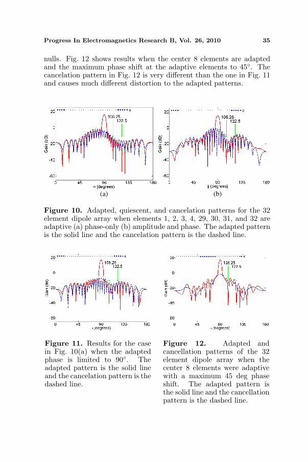
As seen in the previous section, the location of the adaptiveelements in a partially adaptive array determines the shape and gainof the cancelation pattern. Fig. 10 shows the adapted and cancelationpatterns for the 32 element dipole array when elements 1, 2, 3, 4, 29,30, 31, and 32 are adaptive for both phase-only and amplitude and

34 Haupt

Figure 8. Adapted pattern with interference at φ = 106.25◦and 122.5◦ and superimposed on the quiescent pattern. Symmetricelements receive bitwise complements of the 4 out of 8 adaptive phasebits in order to minimize the cancelation pattern peak at φ = 90◦.The adapted pattern is the solid line and the cancelation pattern isthe dashed line.

Figure 9. Adapted weights for Fig. 8.

phase adaptive nulling. Since no limits were placed on the elementweights, the distortion to the adapted pattern is significant.

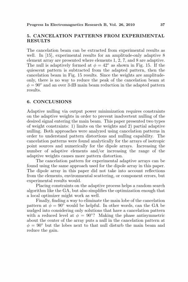
The previous example shows that partial adaptive nulling canproduce unwanted pattern distortion. This distortion can be controlledby placing limits on the adaptive weights or using fewer adaptiveelements. Fig. 11 repeats the previous case but limits the maximumphase shift at the adaptive elements to 90◦. These limits result in muchless distortion to the adapted pattern while still placing the desired


nulls. Fig. 12 shows results when the center 8 elements are adaptedand the maximum phase shift at the adaptive elements to 45◦. Thecancelation pattern in Fig. 12 is very different than the one in Fig. 11and causes much different distortion to the adapted patterns.

(a) (b)

Figure 10. Adapted, quiescent, and cancelation patterns for the 32element dipole array when elements 1, 2, 3, 4, 29, 30, 31, and 32 areadaptive (a) phase-only (b) amplitude and phase. The adapted patternis the solid line and the cancelation pattern is the dashed line.

Figure 11. Results for the casein Fig. 10(a) when the adaptedphase is limited to 90◦. Theadapted pattern is the solid lineand the cancelation pattern is thedashed line.

Figure 12. Adapted andcancellation patterns of the 32element dipole array when thecenter 8 elements were adaptivewith a maximum 45 deg phaseshift. The adapted pattern isthe solid line and the cancellationpattern is the dashed line.

36 Haupt

Figure 13 has the adapted pattern with its cancelation patternwhen 4 elements are adaptive: 1, 2, 31, 32 with 8 bits of phase. Thenulls are placed in the desired directions by a very broad cancelationpattern. It intersects and nulls the quiescent pattern at φ = 106.25◦and φ = 122.5◦. The same case for phase-only nulling appears inFig. 14. Phase-only nulling cause considerably more pattern distortion.Low amplitude weights at the edge elements limit the possible patterndistortion by the cancelation beam.

Figure 13. Amplitude andphase adaptive nulling using 4edge elements. The adaptedpattern is the solid line and thecancelation pattern is the dashedline.

Figure 14. Phase-only adaptivenulling using 4 edge elements.The adapted pattern is the solidline and the cancelation patternis the dashed line.

Figure 15. Plots of the experimental quiescent and adapted patternsfor a null at 45◦. The plot of the cancelation pattern is the differencebetween the adapted and quiescent patterns.


5. CANCELATION PATTERNS FROM EXPERIMENTALRESULTS

The cancelation beam can be extracted from experimental results aswell. In [15], experimental results for an amplitude-only adaptive 8element array are presented where elements 1, 2, 7, and 8 are adaptive.The null is adaptively formed at φ = 42◦ as shown in Fig. 15. If thequiescent pattern is subtracted from the adapted pattern, then thecancelation beam in Fig. 15 results. Since the weights are amplitude-only, there is no way to reduce the peak of the cancelation beam atφ = 90◦ and an over 3 dB main beam reduction in the adapted patternresults.

6. CONCLUSIONS

Adaptive nulling via output power minimization requires constraintson the adaptive weights in order to prevent inadvertent nulling of thedesired signal entering the main beam. This paper presented two typesof weight constraints: 1) limits on the weights and 2) partial adaptivenulling. Both approaches were analyzed using cancelation patterns inorder to understand pattern distortions and nulling capability. Thecancelation patterns were found analytically for the arrays of isotropicpoint sources and numerically for the dipole arrays. Increasing thenumber of adaptive elements and/or increasing the range of theadaptive weights causes more pattern distortion.

The cancelation pattern for experimental adaptive arrays can befound using the same approach used for the dipole array in this paper.The dipole array in this paper did not take into account reflectionsfrom the elements, environmental scattering, or component errors, butexperimental results would.

Placing constraints on the adaptive process helps a random searchalgorithm like the GA, but also simplifies the optimization enough thata local optimizer might work as well.

Finally, finding a way to eliminate the main lobe of the cancelationpattern at φ = 90◦ would be helpful. In other words, can the GA benudged into considering only solutions that have a cancelation patternwith a reduced level at φ = 90◦? Making the phase antisymmetricabout the center of the array puts a null in the cancelation pattern atφ = 90◦ but the lobes next to that null disturb the main beam andreduce the gain.

38 Haupt

REFERENCES

1. Gross, F. B., Smart Antennas for Wireless Communications:With MATLAB, McGraw-Hill, New York, 2005.

2. Compton, R. T., Adaptive Antennas: Concepts and Performance:Prentice-Hall, Philadelphia, Pa., 1987.

3. Monzingo, R. A., R. L. Haupt, and T. W. Miller, Introduction toAdaptive Arrays, NC SciTech Publishing, Raleigh, 2010.

4. Tyler, N., B. Allen, and H. Aghvami, “Adaptive antennas: Thecalibration problem,” IEEE Comm. Mag., Vol. 42, No. 12, 114–122, 2004.

5. Steyskal, H., “Digital beamforming antennas: An introduction,”Microwave Journal, Vol. 30, No. 2, 1–124, 1987.

6. Brookner, E., “Now: Phased-array radars: Past, astoundingbreakthroughs and future trends,” Microwave Journal, Vol. 51,No. 1, 31–48, 2008.

7. Frank, J. and J. D. Richards, “Phased array radar antennas,”Radar Handbook, M. I. Skolnik, Editor, 13.1–13.74, McGraw Hill,New York, 2008.

8. Haupt, R. L. and H. L. Southall, “Experimental adaptive nullingwith a genetic algorithm,” Microwave Journal, Vol. 42, No. 1,78–89, 1999.

9. Baird, C. A. and G. G. Rassweiler, “Adaptive sidelobe nullingusing digitally controlled phase-shifters,” IEEE Transactions onAntennas and Propagation, Vol. 24, No. 5, 638–649, 1976.

10. Haupt, R. L., “Phase-only adaptive nulling with a geneticalgorithm,” IEEE Transactions on Antennas and Propagation,Vol. 45, No. 6, 1009–1015, 1997.

11. Morgan, D., “Partially adaptive array techniques,” IEEETransactions on Antennas and Propagation, Vol. 26, No. 6, 823–833, 1978.

12. Steyskal, H., R. Shore, and R. Haupt, “Methods for null controland their effects on the radiation pattern,” IEEE Transactions onAntennas and Propagation, Vol. 34, No. 3, 404–409, 1986.

13. Shore, R., “Nulling a symmetric pattern location with phase-only weight control,” IEEE Transactions on Antennas andPropagation, Vol. 32, No. 5, 530–533, 1984.

14. FEKO Suite 5.4, EM Software and Systems (www.feko.info), 2008.15. Haupt, R. L., Antenna Arrays: A Computational Approach,

Wiley, New York, 2010.

adaptive nulling with weight constraints … in electromagnetics research b, vol. 26, 23{38, 2010...

Documents