adaptive controller design directly from … · steady-state curve of van de vusse reactor 33. ......
TRANSCRIPT
ADAPTIVE CONTROLLER DESIGN DIRECTLY FROM PLANT
DATA
YAN LI (B. Eng., National University of Singapore, Singapore)
(M. Sc., Mines ParisTech, France)
A THESIS SUBMITTED
FOR THE DEGREE OF MASTER OF ENGINEERING
DEPARTMENT OF CHEMICAL AND BIOMOLECULAR ENGINEERING
NATIONAL UNIVERSITY OF SINGAPORE
2010

ACKNOWLEDGEMENTS
I would like to express my deepest gratitude to my research supervisor, Dr.
Min-Sen Chiu, for his excellent guidance and valuable suggestions during my studies
in the National University of Singapore.
I am also thankful to Dr. Lakshiminarayanan for his valuable advices to my
research work. Special thanks and appreciation are due to my lab mates, Martin
Wijaya Hermanto, Xin Yang, Qinglin Su and Vamsi Krishna Kamaraju, for the
stimulating discussions that we have had and the helps that they have rendered to me.
I would also wish to thank technical and administrative staffs in the Chemical and
Biomolecular Engineering Department for the efficient and prompt help.
I cannot find any words to thank my parents for their unconditional support,
affection and encouragement, without which this research work would not have been
possible.
i

TABLE OF CONTENTS
ACKNOWLEDGEMENTS i
TABLE OF CONTENTS ii
SUMMARY iv
LIST OF TABLES v
LIST OF FIGURES vi
NOMENCLATURE x
CHAPTER 1. INTRODUCTION 1
1.1 Motivations 1
1.2 Contributions 3
1.3 Thesis Organization 4
CHAPTER 2. LITERATURE REVIEW 5
2.1 Adaptive Control for Nonlinear Processes 5
2.2 Direct Data-based Controller Design Methods 11
2.2.1 The VRFT Design Framework 12
2.2.2 Adaptive VRFT design 14
2.3 Nonlinear Internal Model Control (NIMC) 15
CHAPTER 3. ADAPTIVE PID CONTROLLER DESIGN USING EVRFT
METHOD 19
3.1 Introduction 19
ii

iii
3.2 PID Controller Design by VRFT method 20
3.3 Enhanced VRFT Design Method 23
3.4 Examples 24
3.5 Conclusion 42
CHAPTER 4. ADAPTIVE INTERNAL MODEL CONTROLLER DESIGN
USING EVRFT METHOD 43
4.1 Introduction 43
4.2 IMC Controller Design Using VRFT Method 44
4.3 Enhanced VRFT Design Method 47
4.4 Examples 48
4.5 Conclusion 62
CHAPTER 5. CONCLUSIONS AND FURTHER WORK 63
5.1 Conclusions 63
5.2 Suggestions for Further Work 64
APPENDIX A. DERIVATION OF THE 2ND-ORDER REFERENCE MODEL 65
REFERENCES 66

SUMMARY
Controller design for nonlinear dynamic processes has been of great interest in
the chemical industry. Various nonlinear controller design strategies have been
studied in the literature. Among them, adaptive controller is a well-established
solution for this issue. In this thesis, a new adaptive controller design method is
proposed based on the virtual reference feedback tuning (VRFT) method which was
originally developed for linear controller design. This new method is termed as
enhanced VRFT (EVRFT) design to account for the difference from the linear VRFT
method.
In the proposed method, not only a second-order reference model is employed
instead of the first-order reference model commonly used in the linear VRFT design,
but also the parameters of reference model are updated at each sampling instance to
ensure the adaptive nature of the design strategy. In addition, to complete the on-line
adaptation process, the database is updated at each sampling instance by adding the
current process data into it and a relevant dataset is selected from the current database
according to the k-nearest neighborhood criterion.
Two different adaptive controllers are developed implementing the EVRFT
strategy, i.e. an adaptive PID controller and an adaptive Internal Model Controller.
Simulation results show that both proposed controllers give improved control
performance than the linear PID controller designed using VRFT method. They are
also shown to be quite robust in the presence of modeling error and can tolerate
reasonable process noise through simulation studies.
iv

LIST OF TABLES
Table 3.1 Model parameters for polymerization reactor 26
Table 3.2 Steady-state operating condition of polymerization reactor 26
Table 3.3 Tracking errors of servo responses obtained by various
design methods
28
Table 3.4 Tracking errors of servo responses obtained by various
design methods
35
Table 3.5 Tracking errors for EVRFT and VRFT designs for time
delay case
40
Table 4.1 Tracking errors obtained by various design methods 49
Table 4.2 Tracking errors obtained by various design methods 56
Table 4.3 Tracking errors of VRFT and EVRFT designs for time
delay case
58
v

LIST OF FIGURES
Figure 2.1 Diagram of adaptive control scheme 6
Figure 2.2 Reference model 13
Figure 2.3 Feedback control system 13
Figure 3.1 Polymerization reactor 25
Figure 3.2 Input-output data used for constructing the database
(example 1) 27
Figure 3.3 Responses for +50% (top) and -50% (bottom) set-point
changes. Solid line: EVRFT; dotted line: VRFT using 2nd-
order model (A = 0.77); dashed line: VRFT using 1st-order
model (A = 0.95) 29
Figure 3.4 Responses for +50% (top) and -50% (bottom) set-point
changes. Solid line: EVRFT; dotted line: VRFT using 2nd-
order model (A = 0.3); dashed line: VRFT using 1st-order
model (A = 0.5) 29
Figure 3.5 Updating of tuning parameters in EVRFT design (+50%
set-point change) 30
Figure 3.6 Updating of tuning parameters in EVRFT design (-50%
set-point change) 30
Figure 3.7 Responses for +50% (top) and -50% (bottom) set-point
changes by EVRFT design in the presence of modeling
error 31
Figure 3.8 Responses for +50% (top) and -50% (bottom) set-point
changes by EVRFT design in the presence of process noise 32
vi

Figure 3.9 Steady-state curve of van de Vusse reactor 33
Figure 3.10 Input-output data used for constructing the database
(example 2) 34
Figure 3.11 Responses for set-point changes from 1.12 to 1.25 (top)
and to 0.62 (bottom). Solid line: EVRFT; dotted line:
VRFT using 2nd-order model (A = 0.65); dashed line:
VRFT using1st-order model (A = 0.65) 36
Figure 3.12 Responses for set-point changes from 1.12 to 1.25 (top)
and to 0.62 (bottom). Solid line: EVRFT; dotted line: VRF
using 2nd-order model (A = 0.35); dashed line: VRFT
using 1st-order model (A = 0.37) 36
Figure 3.13 Updating of controller parameters in EVRFT design for
set-point change to 1.25 37
Figure 3.14 Updating of controller parameters in EVRFT design for
set-point change to 0.62 37
Figure 3.15 Responses for set-point changes from 1.12 to 1.25 (top)
and to 0.62 (bottom) in the presence of modeling error 38
Figure 3.16 Responses for set-point changes from 1.12 to 1.25 (top)
and to 0.62 (bottom) in the presence of process noise 39
Figure 3.17 Responses for set-point changes from 1.12 to 1.25 (top)
and to 0.62 (bottom) for time delay case. Solid line:
EVRFT; dotted line: VRFT 40
Figure 3.18 Updating of controller parameters in EVRFT design for
set-point change to 1.25 in the presence of time delay 41
Figure 3.19 Updating of controller parameters in EVRFT design for 41
vii

set-point change to 0.62 in the presence of time delay
Figure 4.1 Block diagram of IMC structure 45
Figure 4.2 Responses for +50% (top) and -50% (bottom) set-point
changes. Solid line: EVRFT; dotted line: VRFT using 2nd-
order model (A=0.77); dashed line: VRFT using 1st-order
model (A=0.95) 50
Figure 4.3 Responses for +50% (top) and -50% (bottom) set-point
changes. Solid line: EVRFT; dotted line: VRFT using 2nd-
order model (A = 0.3); dashed line: VRFT using 1st-order
model (A = 0.5) 50
Figure 4.4 Updating of parameter A and IMC parameters (+50% set-
point change) 51
Figure 4.5 Updating of parameter A and IMC parameters (-50% set-
point change) 51
Figure 4.6 Responses for 50% (top) and -50% (bottom) set-point
changes in the presence of modeling error 52
Figure 4.7 Responses for 50% (top) and -50% (bottom) set-point
changes in the presence of process noise 53
Figure 4.8 The catalytic continuous stirred tank reactor 54
Figure 4.9 Steady-state curve of catalytic CSTR 55
Figure 4.10 Input-output data used for constructing the database
(catalytic CSTR) 55
Figure 4.11 Closed-loop responses for set-point changes to 21.5 (top)
and to 19.5 (bottom). Solid line: EVRFT; dotted line:
VRFT using 2nd-order model; dashed line: VRFT using 57
viii

ix
1st-order model
Figure 4.12 Updating of parameter A and IMC parameters for set-point
change to 21.5 59
Figure 4.13 Updating of parameter A and IMC parameters for set-point
change to 19.5 59
Figure 4.14 Responses for set-point changes to 21.5 (top) and to 19.5
(bottom) in the presence of modeling error 60
Figure 4.15 Responses for set-point changes to 21.5 (top) and to 19.5
(bottom) in the presence of process noise 60
Figure 4.16 Responses for set-point changes to 21.5 (top) and to 19.5
(bottom) in the presence of time delay. Solid line: EVRFT;
dotted line: VRFT 61
Figure 4.17 Updating of parameter A and IMC parameters set-point
change to 21.5 in the presence of time delay 61
Figure 4.18 Updating of parameter A and IMC parameters for set-point
change to 19.5 in the presence of time delay 62

NOMENCLATURE
A Tuning parameter of reference closed-loop model
C Controller
AC , , , , , AfC BC bC 1bC 2bC Concentrations
IC , inIC Initiator concentrations
mC , inmC Monomer concentrations
id Distance between ix and x
e Error between set-point and output
F , IF Flow rates
f Low-pass filter
*f Parameter of polymerization reaction
G Process
G~ Model of the process
h Liquid level
1J , 2J Objective functions
PK , , IK DK PID controller parameters
k Number of nearest neighbours
Ik , , , , mfk pk
cTkdTk Parameters of polymerization reaction
1k , , 2k 3k Kinetic parameters
mM Molecular weight of monomer
N Process time-delay
P Process
Q IMC controller
r Set-point
r~ Reference set-point signal
T Reference closed-loop transfer function
u Process input
u~ Virtual input
V Reactor volume
w Weight parameter
x

1w , 2w Flow rates
ix , x Information and query vector
y Process output y Model output in IMC
y Predicted output
Greek Symbols
α ,β Parameters of reference closed-loop model
1α , 2α , 1β ARX model parameters
η Adaptive learning rate
λ IMC filter time constant ρ Vector of discrete time-transfer function
Abbreviations
AIBN Azo-bis-isobutyronitrile
ARX Autoregressive exogenous
CSTR Continuous stirred tank reactor
FA Function approximator
IFT Iterative feedback tuning
IMC Internal model control
ITAE Integral of Time multiplied by Absolute Error
MAE Mean absolute error
MMA Methyl methacrylate
NAMW Number average molecular weight
NN Neural network
PID Proportional-integral-derivative
RMRAC Robust model reference adaptive control
VID2 Virtual input direct design
VRD2 Virtual reference direct design
VRFT Virtual reference feedback tuning
xi

1
Chapter 1
Introduction
1.1 Motivations
In recent years, there is a significant growth in demand for improved process
efficiency due to the competitive market environment. This has driven engineers and
researchers to develop more efficient and reliable techniques for process control.
These techniques, when applied, will not only improve the operating profit of the
controlled process but also ensure its safety during operation and limit its
environmental impacts. In chemical industry, this is especially important since most
of the waste by-products are extremely hazardous to the environment and require
extra treatment before their release. As a result, the study of process control has
become an important subject in chemical engineering research.
In chemical industry, hundreds or even thousands of variables, such as flow
rate, temperature, pressure, levels and compositions are routinely measured and
automatically recorded in historical databases for the purposes of process control,
online optimization or monitoring. Despite of the significant potential benefits that
Chapter 1 Introduction
2
may be obtained from the database, it is generally not a trivial task to extract useful
information and knowledge from the databases. Therefore, “data rich but information
poor” has become a well-known problem in chemical processes. Thus how to extract
relevant information from data and to use this information for controller design
becomes a significant research topic for chemical industry.
Toward this end, several data-based methods for controller design were
developed in the last fifteen years. Spall and Cristion (1998) has developed a
stochastic design framework in which the controller is represented by a function
approximator (FA), such as a polynomial or a neural network, whose parameters are
determined stochastically based on the process measurement. Another direct design
method is the iterative feedback tuning method developed by Hjalmarsson et al.
(1994). However, this method is computationally expansive and it risks to be trapped
in a local optimum when obtaining a solution for the proposed minimization problem,
not to mention its dependence on the trial and error procedure for initialization.
Furthermore, its computation needs unbiased estimates of some variables, which
impose much more stringent requirements during data collection. To overcome this
problem, the virtual input direct design method (VID2, Guardabassi and Savaresi,
1997; Savaresi and Guardabassi, 1998) was the first direct controller design method
without any gradient calculation. Campi et al. (2000) improved and reorganized the
idea of VID2 and renamed the new method as the virtual reference feedback tuning
(VRFT) method. Guardabassi and Savaresi (2000) also developed their new version
called virtual reference direct design (VRD2) which basically follows the same design
principles as VRFT. The VRFT design and its variants share a common feature that
controller parameters are obtained off-line by solving a quadratic optimization
problem based on a set of process input and output data. However, these methods are
Chapter 1 Introduction
3
developed for linear systems and their applications to nonlinear systems are limited.
An adaptive version of the VRFT method (Kansha et al., 2008) is thus proposed to
extend its application to nonlinear processes. This method includes the online update
of the database and selection of relevant dataset to implement its adaptive nature.
However, it still uses a pre-specified reference model which may hinder the
performance of resulting adaptive controller. Therefore, in this thesis, attempts will be
made to develop an enhanced version of the VRFT method to achieve better
performance for nonlinear systems.
1.2 Contributions
In this thesis, an enhanced VRFT (EVRFT) method is developed with
application to adaptive PID controller and adaptive Internal Model Control (IMC)
designs. The main contributions of this thesis are as follows.
(1) Adaptive PID controller design using EVRFT method: In the proposed
EVRFT design, a second-order reference model is employed instead of the
first-order reference model commonly used in the literature. In addition, other
than the update of database and relevant dataset, the parameters in the
reference model will also be updated at each sampling instance to further
improve the resulting control performance.
(2) Adaptive IMC controller design using EVRFT method: IMC is a powerful
controller design strategy for the open-loop stable dynamic systems. However,
the performance of IMC controller will degrade or become unstable when it is
applied to nonlinear processes with a range of operating conditions. In the
proposed IMC design, the EVRFT design is applied to update the IMC
controller at each sampling instance. Again, the reference model is updated at

Chapter 1 Introduction
4
each sampling instance, in addition to the update of database and relevant
dataset.
1.3 Thesis Organization
The thesis is organized as follows. Chapter 2 comprises the literature review
of nonlinear process control. In Chapter 3, an enhanced version of the VRFT method
is developed to design an adaptive PID controller. Moreover, by incorporating the
enhanced VRFT design framework into IMC design, an adaptive IMC controller for
nonlinear processes is proposed in Chapter 4. Finally, the general conclusions from
the present work and suggestions for future work are given in Chapter 5.

Chapter 2
Literature Review
This chapter examines the research work that has been conducted in the field
of nonlinear process control. An overview of adaptive controller design method is
presented. Following that, the detailed development of the VRFT method will be
discussed. Finally, various nonlinear IMC designs will be reviewed.
2.1 Adaptive Control for Nonlinear Processes
In chemical and biochemical industries, majority of the processes are
inherently nonlinear, however most controller design techniques are based on liner
control techniques to deal with such systems. The prevalence of linear control
strategies is partly due to the fact that, over the normal operating region, many of the
processes can be approximated by linear models, which can be obtained by the well-
established identification methods and the available input and output process data. In
addition, the theories for the stability analysis of linear control systems are quite well
5

Chapter 2 Literature Review
developed so that linear control techniques are widely accepted. However, due to the
nonlinear nature of most chemical processes, linear control design methodologies may
not be adequate to achieve a good control performance for these processes. This has
led to an increasing interest in the nonlinear controller design for the nonlinear
dynamic processes. Adaptive controller is a well-established solution for nonlinear
process control and its concept will be used throughout this thesis.
Figure 2.1 Diagram of adaptive control scheme
Research in adaptive control has a long and vigorous history. The
development of adaptive control started in the 1950’s with the aim of developing
adaptive flight control systems. With the progressing of control theories and computer
technology, various adaptive control methodologies were proposed for process control
in the last three decades. Åström (1983), Seborg et al. (1986) and Åström and
Wittenmark (1995) gave detail reviews of the theories and application of adaptive
control. Most adaptive methodologies integrate a set of techniques for automatic
adjustment of controller parameters in real time in order to achieve or to maintain a
6

Chapter 2 Literature Review
desired level control performance when the dynamic characteristics of the process are
unknown or vary in time. The diagram of adaptive control concept is depicted in
Figure 2.1. There are three main technologies for adaptive control: gain scheduling,
model reference control, and self-tuning regulators. The purpose of these methods is
to find a convenient way of changing the controller parameters in response to changes
in the process and environment dynamics.
Gain scheduling is one of the earliest and most intuitive approaches for
adaptive control. The idea is to find process variables that correlate well with the
changes in process dynamics. It is then possible to compensate for process parameter
variations by changing the parameters of the controller as function of the process
variables. The advantage of gain scheduling is that the parameters can be changed
quickly in response to changes in the process dynamics. It is convenient especially if
the process dynamics in a well-known fashion on a relatively few easily measurable
variables. Gain scheduling has been successfully applied to nonlinear control design
for process industry (Åström and Wittenmark, 1995). One drawback of gain
scheduling is that it is open-loop compensation without feedback. Another drawback
of gain scheduling is that the design is time consuming. A further major difficulty is
that there is no straightforward approach to select the appropriate scheduling variables
for most chemical processes.
Model reference control is a class of direct self-tuners since no explicit
estimate or identification of the process is made. The specifications are given in terms
of “reference model” which tells how the process output ideally should respond to the
command signal. The desired performance of the closed-loop system is specified
through a reference model, and the adaptive system attempts to make the plant output
match the reference model output asymptotically.
7

Chapter 2 Literature Review
The third class of adaptive control is self-tuning controller. The general
strategy of this controller is to estimate model parameters on-line and then adjust the
controller settings based on current parameter estimate (Åström, 1983). In the self-
tuning controller, at each sampling instant the parameters in an assumed dynamic
model are estimated recursively from input-output data and controller setting is then
updated. The whole control strategy can be divided into three steps: (i) information
gathering of the present process behavior; (ii) control performance criterion
optimization; (iii) adjustment of the controller parameters. The first step implies the
continuous determination of the actual condition of the process to be controlled based
on measurable process input and output and appropriate approaches selected to
identify the model parameters. Various types of model identification can be
distinguished depending on the information gathered and the method of estimation.
The last two steps calculate the control loop performance and the decision as to how
the controller will be adjusted or adapted. These characteristics make self-tuning
controller very flexible with respect to its choice of controller design methodology
and to the choice of process model identification (Seborg et al., 1986).
In the past two decades, many research efforts have focused on the
development of intelligent control algorithms that can be applied to complex
processes whose dynamics are poorly modeled and/or have severe nonlinearities.
(Stephanopoulos and Han, 1996; Linkens and Nyongesa, 1996). Because neural
networks (NNs) have the capacity to approximate any nonlinear function to any
arbitrary degree of accuracy, NNs have received much attention in the area of
adaptive control. Perhaps the most significant work of the application of NNs in
adaptive control is that of Narendra and Parthasarathy (1990) who investigated
adaptive input-output neural models in model reference adaptive control structures.
8
Chapter 2 Literature Review
Hernandez and Arkun (1992) studied control-relevant properties of neural network
model of nonlinear systems. Jin et al. (1994) used recurrent neural networks to
approximate the unknown nonlinear input-output relationship. Based on the dynamic
neural model, an extension of the concept of the input-output linearization of discrete-
time nonlinear systems is used to synthesize a control technique under model
reference control framework. te Braake et al. (1998) provided a nonlinear control
methodology based on neural network combined with feedback linearization
technique to transform the nonlinear process into an equivalent linear system in order
to simplify the controller design problem. Recently, some researchers have
constructed stable NN for adaptive control based on Lyapunov’s stability theory
(Lewis et al., 1996; Polycarpou, 1996; Ge et al., 2002). One main advantage of these
schemes is that the adaptive laws are derived based on the Lyapunov synthesis
method and therefore guarantee the stability of the control systems. While neuro-
control techniques are suited to control an unknown nonlinear dynamic process, it is
generally difficult to present the control law in simple analytical form. Also, a
nonlinear optimization routine is required to determine the control input, which may
lead to the problems of large computational efforts and poor convergence. To
alleviate this problem, an innovative real-time model reference neural control system
is developed by Pérez et al. (2009). This neural controller allows one to assimilate the
complex system dynamics to a simple first-order linear system, which can be easily
controlled by a conventional PID controller.
The PID controllers have received widespread use in the process industries
primarily because of its simple structure, ease of implementation, and robustness in
operation. Due to these advantages, several adaptive PID controller designs have been
developed in recent years. For example, Riverol and Napolitano (2000) proposed an
9

Chapter 2 Literature Review
adaptive PID controller whose parameters are adjusted on-line by a neural network,
while Chen and Huang (2004) designed adaptive PID controller based on the
instantaneous linearization of a neural network model. Altinten et al. (2004) applied
the genetic algorithm to the optimal tuning of a PID controller on-line. Bisowarno et
al. (2004) applied two adaptive PI control strategies for reactive distillation. Andrasik
et al. (2004) made use of a hybrid model consisting of a neural network and a
simplified first-principle model to design a neural PID-like controller. Yamamoto and
Shah (2004) developed an adaptive PID controller using recursive least squares for
on-line identification of multivariable system. Shahrokhi and Baghmisheh (2005)
designed an adaptive IMC-PID controller based on the local models estimated by the
recursive least squares method to control a fixed-bed reactor. Similar approaches for
adjusting PID controller parameters on-line were investigated based on the multiple
linearized models obtained by factorization algorithm and lazy learning identification
method at each sampling instance (Ho et al., 1999; Alpbaz et al., 2006; Pan et al.,
2007). Another multi-model adaptive strategy for PID controllers was proposed based
on a set of simple linear dynamic models where each model has the same structure but
different values of the model parameters (Böling et al., 2007). Yu et al. (2007)
extended the adaptive PID control strategy to multivariable nonlinear systems with
unknown dynamics by proposing a stable self-learning PID control scheme based on a
neural network (NN) model of the plant. In these works, basically, the parameters of
the process model are updated with respect to the current process condition and then
PID parameters are computed by the corresponding adaptation algorithm and
implemented.
In this thesis, an adaptive PID controller design strategy using directly process
data will be developed in Chapter 3 with EVRFT as the adaptation algorithm.
10
Chapter 2 Literature Review
2.2 Direct Data-based Controller Design Methods
Designing controllers directly based on a set of measured process input and
output data, without resorting to the identification of a process model, is an attractive
option for process control application. Such ‘direct’ data-based design techniques are
conceptually more natural than model-based designs where the controller is designed
on the basis of an estimated model of the process, because the former directly targets
the final goal of tuning the parameters of a given class of controllers. However,
despite the appeal of direct data-based design methods, very few genuine direct
design techniques have been proposed in literature
Hjalmarsson et al. (1994) developed iterative feedback tuning (IFT) method
with promising result for real application (1998). However, IFT may require
considerable computational time to obtain a solution with a risk of being a local
optimum in the proposed minimization problem, not to mention its dependence on the
trial and error procedure for initialization. Furthermore, its computation needs
unbiased estimates of some variables, which impose much more stringent
requirements on the experiment. As a result, the experiment required for IFT is
typically complicated.
Spall and Cristion (1998) proposed a stochastic approach for adaptive control
using a function approximator (FA) to calculate the action needed from the controller.
FA can be a polynomial or an artificial neural network, whose parameters are updated
repeatedly in accordance with the minimization of a cost function. However, since a
plant model is not available, the gradient of this cost function has to be evaluated by
simultaneous perturbation stochastic approximation instead of quadratic methods.
Thus, the computational burden of this method is very high due to the iterations and
the convergence of the trained parameters may not be guaranteed.
11

Chapter 2 Literature Review
To alleviate the aforementioned drawbacks, Campi and Lecchini (2000, 2002)
proposed the virtual reference feedback tuning method (VRFT). VRFT stems from the
idea of virtual input direct design (VID2) (Guardabassi and Savaresi, 1997; Savaresi
and Guardabassi, 1998), but in a better-organized form. This methodology is simple
and directly calculates the feedback controller parameters from the available process
input and output data without the need of model identification. Under this tuning
framework, only the specification of desired reference model is required. Nakamoto
(2005) extended this controller design technique to multivariable systems and showed
a chemical process application.
An adaptive version of the VRFT method (Kansha et al., 2008) is proposed to
extend its application to nonlinear processes. In this adaptive VRFT design, the off-
line database employed in the conventional VRFT design is continuously updated by
adding the current process data into the database. Furthermore, PID parameters are
determined by the VRFT design at each sampling instance using the relevant dataset
selected from the current database based on k-nearest neighborhood criterion. An
enhanced version of this method will be developed in Chapter 3 by using a second-
order reference model with update in its parameter as well.
2.2.1 The VRFT design framework
The VRFT method approximately solves a model-reference problem in
discrete time as depicted in Figure 2.2, where the reference model ( )1−zT describes
the desired behavior of the closed-loop system consisting of a linear time-invariant
process ( )1−zP and a parameterized controller ( )θ;1−zC as shown in Figure 2.3. Let
us assume that ( )1−zP
( )
is unknown and only a set of process input and output data,
( ){ }kku = n~1 and{ }kky 1= n~ , have been collected from e experime th nt on the plant and
12

Chapter 2 Literature Review
that a reference model ( )1−zT has been chosen. The design goal is to solve θ , a
vector consisting of the controller parameters, such that the feedback control sys em
in Figure 2.2 behaves as closely as possible to the pre-specified reference model
t
( )1−zT .
Figure 2.2 Reference Model
Figure 2.3 F
u
eedback Control System
Given the meas red output signal ( ){ } nkky ~1= , the corresponding reference
( )} nkkr ~1{~ = in Figure 2.2 is obtained by signal
( ) ( ) ( )1111~ − = Tzr −−− zyz (2.1)
where ( )1~ −zr and ( )1−zy are the Z-transforms of discrete time signals ( ){ } nkkr ~1~
= and
( ){ }kky spect ( ){ } nkkr ~1n~1= , re ively. ~= is called ‘virtual’ reference signal because it does
s not used in the generation of ( )ky . However, it
plays a pivotal role in the VRFT framework in that the fundamental idea of the VRFT
framework is to treat ( ){ } nkky ~1= as the desired output of the feedback system when
the reference signal d by
not exist in reality and in fact i
s specif
t wa
iei ( ){ } nkkr ~1~
= . As a consequence, given error
( ) ( ) (ky− )signal krk = ~ , the controller output ( )ku~e is calculated as:
13

Chapter 2 Literature Review
( ) ( ) ( ){ ( )}1111 ~;~ −− zy −−− = zrzCzu θ (2.2)
where
( )1~ −zu is the Z-tr e siansforms of discrete tim gnal ( ){ } nkku ~1~
= .
It is noted that, even though the process dynamics ( )1−zP is not known, when
the process is fed by ( )ku , i.e. the measured input sign era ate , i.e. the
corresp
l, it gen s ( )ky
onding measured output signal. Therefore, a good controller generates ( )ku
when the error signal is given by ( )ke . The idea is then to search for ( )θC whose
output ( )ku~ matches ( )ku as closely as possible. Hence, the controller design task
reduces to the following minimization problem:
( )
;1−z
( ) ( ){ }∑ −=n
kukuJ 21
~1nθ (2.3) =kn 1
miθ
If the controller is given by ( ) ( )θρθ 11; −− = zzC T where ( )1−zρ is a vector of
discrete nsfer function, it can -time tra en that Eq. (2.3) is quadratic inbe se θ .
Consequently, the controller parameter es Eq. ( n be explicitly
obtained by the classical least-square technique. As a result, the VRFT des n
framework effectively recasts the problem of designing a model-reference feedback
controller into a standard system-identification problem. More detailed discussions on
the VRFT can be found in Campi et al. (2000, 2002).
2.2.2 Adaptive VRFT design
*θ which minimiz 2.3) ca
ig
In the conventional VRFT design, the database collected from an off-line
as a result the resulting controller is expected to
perform well in the vicinity of operating
open-loop experiment is utilized and
space close to the operating condition where
this dataset is generated. To extend the VRFT design to nonlinear systems, one
possible approach is to augment the original off-line database by adding the current
14

Chapter 2 Literature Review
process data at each sampling instance so that the expanded database can cover new
operating space where its dynamics is not available in the construction of original
database. This expanded database is subsequently used to obtain PID parameters by
VRFT design at each sampling instance. In doing so, the relevant data in the expanded
database that corresponds to the current process condition is first determined by using
the k-nearest neighborhood criterion based on the following distance measure:
( ) ii xkxd −−= 1 (2.4)
where ⋅ denotes the Euclidean norm, ( ) ( )[ ]Tiuiyx = is a pair of input and output i
data in the present dataset, and ( )1−kx is a vector with similar definition for the input
nstance. and output data at the (k-1)-th sampling i
By using Eq. (2.4), those ix cor
hich the constrained least squares
problem
ear Internal Model Control (NIMC)
al Model Control (IMC) proposed by Garcia and Morari (1982) is a
ic systems (Morari
and Za
responding to the k smallest id are selected as
the relevant data in the current database, by w
discussed in the subsection 2.2.1 is solved to calculate PID parameters for
the current sampling instance. This design procedure repeats at the next sampling
instance when the database for VRFT design is further updated by the corresponding
process data.
2.3 Nonlin
Intern
powerful controller design strategy for the open-loop stable dynam
firiou, 1989). This is mainly due to two reasons. First, integral action is
included implicitly in the controller because of the IMC structure. Moreover,
plant/model mismatch can be addressed via the design of the robustness filter. IMC
design is expected to perform satisfactorily as long as the process is operated in the
15

Chapter 2 Literature Review
vicinity of the point where the linear process model is obtained. However, the
performance of IMC controller will degrade or even become unstable when it is
applied to nonlinear processes with a range of operating conditions.
To extend the IMC design to nonlinear processes, various nonlinear IMC
schemes have been developed in the literature. For instance, Economou et al. (1986)
provide
n in Bhat and McAvoy
(1990)
d a nonlinear extension of IMC by employing contraction mapping principle
and Newton method. However, this numerical approach to nonlinear IMC design is
computationally demanding. Calvet and Arkun (1988) used an IMC scheme to
implement their stat-space linearization approach for nonlinear systems with
disturbance. A disadvantage of the state-space linearization approach is that an
artificial controlled output is introduced in the controller design procedure and cannot
be specified a priori. Another drawback of this method is that the nonlinear controller
requires state feedback (Henson and Seborg, 1991a). Henson and Seborg (1991b)
proposed a state-space approach and used nonlinear filter to account for plant/model
mismatch. However, their method relied on the availability of a nonlinear state-space
model, which may be time-consuming and costly to obtain.
Another popular design method for implementing nonlinear IMC schemes is
based on the neural networks. In the earlier methods give
and Hunt and Sbarbaro (1991), two NN were used in the IMC framework,
where one NN was trained to represent the nonlinear dynamics of process, which was
then used as the IMC model, while another NN was trained to learn the inverse
dynamics of the process and was employed as the nonlinear IMC controller. Because
IMC model and controller were built by separate neural networks, the controller
might not invert the steady-state gain of the model and thus steady-state offset might
not be eliminated (Nahas et al., 1992). Moreover, these control schemes do not
16

Chapter 2 Literature Review
provide a tuning parameter that can be adjusted to account for plant and model
mismatch. To ensure offset-free performance, Nahas et al. (1992) developed another
NN based nonlinear IMC strategy, which consists of a model inverse controller
obtained from a neural network and a robustness filter with a single tuning parameter.
In this control strategy, a numerical inversion of neural network process model was
proposed instead of training neural networks on the process inverse. Aoyama et al.
(1995) proposed a method using control-affine neural network models. Two neural
networks were used in this approach: one for the model of the bias or drift term, and
one for the model of the steady-state gain. As the process is approximated by a
control-affine model, the inversion of process model is simply obtained by
algebraically inverting the process model.
However, the above nonlinear IMC designs sacrifice the simplicity associated
with linear IMC in order to achieve improved performance. This is mainly due to the
use of computationally demanding analytical or numerical methods and neural
networks to learn the inverse of process dynamics for the necessary construction of
nonlinear process inverses. To overcome these difficulties, a promising approach has
been proposed to yield a flexible nonlinear model inversion (Doyle et al., 1995; Harris
and Palazoglu, 1998). This controller synthesis scheme based on partitioned model
inverse retains the original spirit and characteristics of conventional (linear) IMC
while extending its capabilities to nonlinear systems. When implemented as part of
the control law, the nonlinear controller consists of a standard linear IMC controller
augmented by an auxiliary loop of nonlinear “correction”. The fact that only a linear
inversion is required in the synthesis of this controller is the most attractive feature of
this scheme. However, Volterra model derived using local expansion results such as
Carleman linearization is accurate for capturing local nonlinearities around an
17

Chapter 2 Literature Review
18
operating point, but may be erroneous in describing global nonlinear behavior (Maner
et al., 1996). Harris and Palazoglu (1998) proposed another nonlinear IMC scheme
based on the functional expansion models instead of Volterra model. However,
functional expansion models are limited to fading memory systems and the radius of
convergence is not guaranteed for all input magnitudes. Consequently, the resulting
controller gives satisfactory performance only for a limited range of operation. This
limitation restricts the implementation of these models in practice (Xiong and Jutan,
2002).
Shaw et al. (1997) used recurrent neural network (RNN) within the partitioned
model inverse controller synthesis scheme in IMC framework and showed that this
strategy
e the parameters of the
IMC co
sed in Chapter 4.
provided an attractive alternative for NN-based control application.
Maksumov et al. (2002) investigated the first experimental application of this control
strategy using NN as a nonlinear model and a linear ARX model. However, one
fundamental limitation of these global approaches for modeling is that the on-line
update of these models is not straightforward when the process dynamics are moved
away from the nominal operating space. Evidently, this will interrupt the plant
operation when these models are used in the controller design.
To circumvent the aforementioned drawback, an adaptive IMC controller is
proposed based on just-in-time learning (JITL) technique wher
ntroller as well as its filter parameter are updated based on the information
provided by the JITL (Cheng and Chiu, 2007). Kalmukale et al. (2007) developed
another partitioned model-based IMC design strategy for a class of nonlinear systems
that can be described by the JITL modeling technique.
In this thesis, a new adaptive IMC design strategy using Enhanced Virtual
Reference Feedback Tuning (EVRFT) method is propo
Chapter 3
Adaptive PID Controller Design
Using EVRFT Method
3.1 Introduction
Model-based controller design techniques have been receiving much research
attention in the past several decades. Among them, a number of PID tuning formulas
such as ITAE performance index, direct synthesis design method and Internal Model
Control (IMC) design, are well established in the literature. These model-based
controller design methods generally follow a two-step procedure: the first step is to
identify a process transfer function model with a pre-specified model structure, for
example a first-order-plus-delay model, which gives a reasonably good modeling
accuracy; the second step is to design the controller based on the model thus obtained.
Another interesting alternative for controller design is the data-based methods.
For example, the Virtual Reference Feedback Tuning (VRFT) method developed by
Campi et al. (2000, 2002) is a direct data-based method that determines the
19

Chapter 3 Adaptive PID Controller Design Using EVRFT Method
parameters of a controller by using a set of input and output data from the process
without resorting to the identification of a process model. However, this design
framework is originally developed for linear systems. As a result, controllers designed
under this framework have limited performance for nonlinear processes. An adaptive
version of the VRFT method (Kansha et al., 2008) is thus proposed to extend its
application to nonlinear processes. In this adaptive VRFT design, the off-line database
employed in the conventional VRFT design is continuously updated by adding the
current process data into the database. Furthermore, PID parameters are determined
by the VRFT design at each sampling instance using the relevant dataset selected
from the current database based on k-nearest neighborhood criterion.
In this chapter, an enhanced version of the adaptive VRFT method is
developed to design an adaptive PID controller. In the proposed enhanced VRFT
design, a second-order reference model is employed instead of the first-order
reference model commonly used in the previous work. In addition, other than the
update of database and relevant dataset, the parameters in the reference model will
also be updated at each sampling instance. Simulation results are presented to
illustrate the proposed design method and a comparison with conventional VRFT
design is made.
3.2 PID Controller Design by VRFT Method
In this section, the detailed formulation for PID controller design using VRFT
method with a second-order reference model is discussed.
Consider a PID controller given by:
( ) ( ) ( ) ( )[ ] ( )
( ) ( ) ( )[ 21211−+−−+ ]+−−+−=
kekekeKkeKkekeKkuku
D
IP (3.1)
20

Chapter 3 Adaptive PID Controller Design Using EVRFT Method
where is the manipulated value at the k-th sampling instance, is the error
between process output and its set-point at the k-th sampling instance, and ,
and are PID parameters. The corresponding
( )ku
DK
( )ke
PK
IK ( )θ;1−zC will be:
( ) ( 11
1 11
; −−
− −+ )−
+= zKz
KKzC DI
pθ (3.2)
In VRFT design framework, the reference model ( )1−zT is specified by the
following second-order closed-loop transfer function derived in Appendix A:
( )⎩⎨⎧
−−=+−=
+−+
== −−
−−−
−
−−
AAAAAAA
wherezAAz
zzzrzyzT
N
lnln1
21)()()( 2221
11
1
11
βαβα (3.3)
where A is the tuning parameter related to the speed of the response and N is the
process time delay.
To design a PID controller by the VRFT method, the virtual input ( )1~ −zu is
calculated by Eqs. (2.1), (2.2), (3.2) and (3.3) to obtain
( ) ( )( ) ( 1
11
112211
11 211
1)(~ −
−−−
−−−−−−
−−
++−+−
⎥⎦⎤
⎢⎣⎡ −+
−+= zy
zzzzzAAzzK
zK
Kzu N
N
DI
P βαβα )
)
(3.4)
Define ( 1~ −Φ z as follows:
( ) )()( 111 −−− +=Φ zuzz βα (3.5)
The following equation can be obtained from Eqs. (3.4) and (3.5)
( ) ( ) ( 11
112211
11 211
1)(~ −
−−
−−−−−−
−− +−+−
⎥⎦⎤
⎢⎣⎡ −+
−+=Φ zy
zzzzAAzzK
zK
Kz N
N
DI
Pβα ) (3.6)
Equation (3.5) can be rewritten as:
( ) ( ) ( )1−+=Φ kukuk βα (3.7)
Equation (3.6) can then be rewritten as:
( ) ( )kKk Ψ=Φ~ (3.8)
where
21

Chapter 3 Adaptive PID Controller Design Using EVRFT Method
( ) ( ) ( ) ( )[ TDIP kkkk ΨΨΨ=Ψ ]
]
(3.9)
[ DIP KKKK = (3.10)
( ) ( ) ( ) ( ) ( 1)1(21 2 −−−−+++−++=Ψ kykyNkyANkAyNkykP βα ) (3.11)
(3.12) ( )( ) ( )
( ) ( ) ( ) ( )( ) ( ) ( ) ( ) ( ) ( )⎪
⎪
⎩
⎪⎪
⎨
⎧
≥++−++−−++
=++−−+=+−+
=Ψ
∑−
=
1
1
2 21121
111220)ln1(1
N
i
I
NforkyikyANkyANky
NforkykyAkyNforkyAAky
k
β
β
( ) ( ) ( ) ( ) ( ) ( )
( ) ( ) ( ) ( ) ( 212
121212
2
−+−−+−−+−
−+++++−++=Ψ
kykykyNkyA
NkyAANkyANkykD
ββαα ) (3.13)
Equation (2.3) is then expressed by
( ) ( ) ( ){ }
2
2
11
1min
1min
Ψ−Φ=
Ψ−Φ= ∑=
Kn
kKkn
KJ
K
n
kK (3.14)
subject to the following constraints of PID controller parameters:
0,,0,, >< DIPDIP KKKorKKK (3.15)
where
( ) ( ) ( )( ) ( ) ( )( ) ( ) ( )⎥
⎥⎥
⎦
⎤
⎢⎢⎢
⎣
⎡
ΨΨΨΨΨΨΨΨΨ
=Ψnnn
DDD
III
PPP
L
L
L
212121
(3.16)
( ) ( )[ n ]ΦΦ=Φ L1 (3.17)
Consequently, PID parameters are obtained by solving the constrained least
square problem as stated above. It is evident that this solution not only depends on the
database for VRFT design but also the design parameter A in the reference model.
22

Chapter 3 Adaptive PID Controller Design Using EVRFT Method
3.3 Enhanced VRFT Design Method
The proposed enhanced VRFT design method (EVRFT) is focused on the
updating of the reference model while keeping the basic VRFT framework described
in section 3.2. The objective of this updating procedure is to enhance the capability of
VRFT design to cope with the variation of process dynamics resulting from the
process nonlinearity. This is achieved by updating the tuning parameter A in the
reference model at each sampling instance as it has a direct impact on the PID
parameters calculated using the VRFT method.
The objective of adjusting reference model parameter A is to minimize the
following quadratic function:
( ) ( ) ( ) ( )[ ] ( ) ( )[{ }222 11ˆ11
21
−−++−+−= kukuwkykrwkJ ]
]
(3.18)
where is a weight parameter and [ 1,0∈w ( )1ˆ +ky is the predicted output using the
reference model at the (k+1)-th sampling instance which can be calculated by:
( ) ( ) ( ) ( ) ( )1121ˆ 2 −−+−+−−=+ NkrNkrkyAkAyky βα (3.19)
By the steepest descent method, the updating algorithm is derived as:
( ) ( ) ( ) ( )( )kA
kJkkAkA∂∂
−=+ 21 η (3.20)
where ( )kη is the learning rate.
In the proposed design, the following rules are used to update the learning rate:
(i) if the increment of is more than a threshold, the tuning parameter A remains
unchanged and the learning rate is decreased by a factor , i.e.
2J
decl ( ) ( )klk decηη =+1 ;
(ii) if the absolute value of the change of is smaller the threshold, only the
parameter A is updated; otherwise, (iii) the parameter A is updated and the learning
rate is increased by a factor , i.e.
2J
incl ( ) ( )kk lincηη =+1 .
23

Chapter 3 Adaptive PID Controller Design Using EVRFT Method
The following outlines the computational algorithm for the proposed EVRFT
design of adaptive PID controller.
Step 1 The process input (u(k)) and output (y(k)) data that characterize the dynamics
of nonlinear system are assumed to be available and the off-line database for
EVRFT design is constructed as ( ) niix ~1= ;
Step 2 At the k-th sampling instance, based on the current database for EVRFT
design, the relevant dataset is selected according to Eq. (2.4) and then the PID
parameters are calculated by solving the minimization problem given by Eq.
(3.14) subjected to the constraint Eq. (3.15). The manipulated variable ( )ku is
obtained by Eq. (3.1).
Step 3 The database for EVRFT design is augmented by appending the current
process data and ( )ky ( )ku , while the tuning parameter A is updated using Eq.
(3.20) whenever required according to the empirical rules mentioned above.
Step 4 Set and go to Step 2. 1+= kk
3.4 Examples
Example 1 Considering a continuous polymerization reaction that takes place
in a jacketed CSTR (Doyle et al., 1995), as depicted in Figure 3.1. In the reactor, an
isothermal free-radical polymerization of methyl methacrylate (MMA) is carried out
using azo-bis-isobutyronitrile (AIBN) as initiator and toluene as solvent. The control
objective is to regulate the product number average molecular weight (NAMW) by
manipulating the flow rate of the initiator ( ), i.e., NAMW is the process output
and is as process input u . Under the following assumptions: (i) isothermal
operation; (ii) perfect mixing; (iii) constant heat capacity; (iv) no polymer in the inlet
IF y
IF
24

Chapter 3 Adaptive PID Controller Design Using EVRFT Method
stream; (v) no gel effect; (vi) constant reactor volume; (vii) negligible initiator flow
rate (in comparison with monomer flow rate); and (viii) quasi-steady state and long-
chain hypothesis, the dynamics of the reactor can be described by the following
equations:
VCCF
PCkkt
C mmmfmp
m in)(
)(d
d0
−++−=
VFCCF
Ckt
C in IIIII
I
dd −
+−=
VFD
PCkPkkdt
dDmfTT mdc
00
20
0 )5.0( −++=
VFDPCkkM
dtdD
mfpm m1
01 )( −+=
0
1
DDy = (3.21)
where 5.0
II0
*2
⎥⎥⎦
⎤
⎢⎢⎣
⎡
+=
cd TT kkCkfP . The model parameters and steady-state operation
condition are given in Tables 3.1 and 3.2.
Figure 3.1 Polymerization reactor
25

Chapter 3 Adaptive PID Controller Design Using EVRFT Method
Table 3.1 Model parameters for polymerization reactor
cTk = 10103281.1 × h)/(kmolm3 F = 1.00 /hm3
dTk = 11100930.1 × h)/(kmolm3 V = 0.1 3m
Ik = 1100225.1 −× L/h inIC = 8.0 3kmol/m
pk = 6104952.2 × h)/(kmolm3mM = 100.12 kg/kmol
mfk = 3104522.2 × h)/(kmolm3inmC = 6.0 3kmol/m
*f = 0.58
Table 3.2 Steady-state operating condition of polymerization reactor
mC = 5.506774 3kmol/m 1D = 49.38182 3kmol/m
IC = 0.132906 3kmol/m IFu = = 0.016783 /hm3
0D = 0.0019752 3kmol/m y = 25000.34 kg/kmol
To obtain the database for EVRFT design, an open-loop test is conducted by
introducing random steps around the nominal value of process input and the
corresponding input and output data are given in Figure 3.2. The process input and
output are scaled by
IF
016783.0016783.0~ −
=uu and
34.2500034.25000~ −
=yy respectively.
To proceed the EVRFT design of adaptive PID controller, the tuning
parameters specified are as follows: the initial value of parameter A = 0.6, initial
learning rate 002.0=η , weight parameter used in the objective function Eq. (3.18)
given by , the updating parameters for learning rate 7.0=w 02.1=incl and ,
and the number of data points in the relevant dataset is set to 1200.
55.0=decl
26

Chapter 3 Adaptive PID Controller Design Using EVRFT Method
Figure 3.2 Input-output data used for constructing the database (example 1)
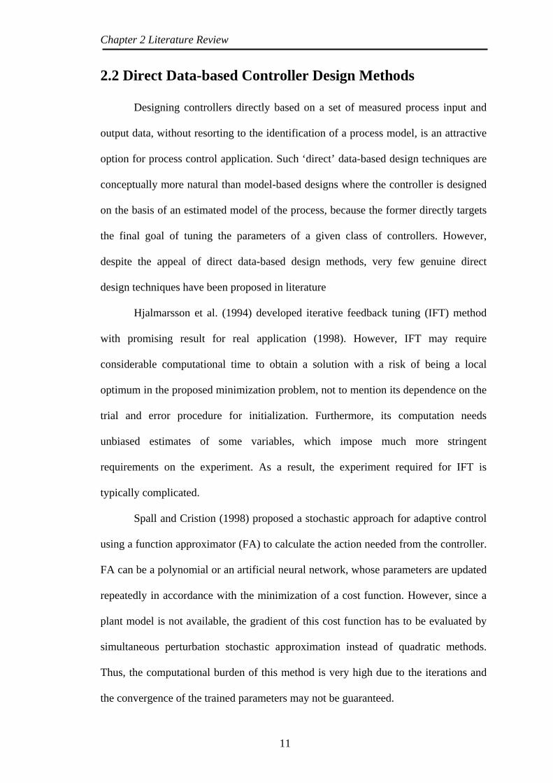
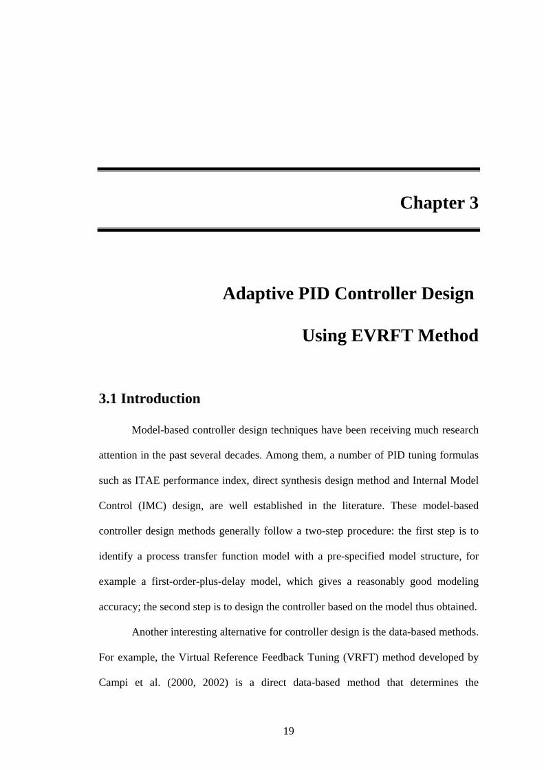
To evaluate the performance of the adaptive PID controller designed using
EVRFT method, +50% and -50% set-point changes are conducted, as illustrated in
Figures 3.3 and 3.4. Figures 3.5 and 3.6 show the updating of tuning parameter A and
PID parameters in EVFRT design for the abovementioned servo responses.
Since polymerization reactor is operated in a wide range of operating space
between the set-points 12500 and 37500, a linear PID controller cannot provide
satisfactory control performance as a result of process nonlinearity. To better illustrate
this point, four PID controllers designed using VRFT method with first-order and
second-order reference models are developed. To match the performance of EVRFT
design for +50% set-point change as closely as possible, two PID controllers are
obtained by VRFT design using tuning parameters A = 0.95 and A = 0.77 for the first-
order and second-order reference models, respectively. From Figure 3.3, it can be
27

Chapter 3 Adaptive PID Controller Design Using EVRFT Method
seen that both adaptive PID controller designed using EVRFT method and the PID
controller designed using VRFT method with second-order reference model
outperform the PID controller designed using VRFT method with first-order reference
model. Although VRFT design using second-order reference model is able to match
the EVRFT design for +50% set-point change, it gives slower performance than the
EVRFT design for -50% set-point change.
Similarly, to match the performance of EVRFT design for -50% set-point
change as closely as possible, another two PID controllers are obtained by VRFT
design using tuning parameters A = 0.5 and A = 0.3 for the first-order and second-
order reference models, respectively. Figure 3.4 shows that, while comparable
performances for -50% set-point change are observed for both VRFT and EVRFT
designs, EVRFT design gives better performance than the two VRFT designs for
+50% set-point change. Table 3.3 summarizes the tracking errors of the
abovementioned servo responses.
Table 3.3 Tracking errors obtained by various design methods
VRFT design using 1st-order model
VRFT design using 2nd-order model
% improvement (based on VRFT design using 2nd-order model)
Set-point change
A=0.95 A=0.5 A=0.77 A=0.3
EVRFT design
A=0.77 A=0.3+50% 1836 2920 868 2479 921 -6.1% 62.9% -50% 2984 356 1465 387 362 75.3% 6.4%
28

Chapter 3 Adaptive PID Controller Design Using EVRFT Method
Figure 3.3 Responses for +50% (top) and -50% (bottom) set-point changes. Solid line: EVRFT; dotted line: VRFT using 2nd-order model (A = 0.77); dashed line:
VRFT using 1st-order model (A = 0.95)
Figure 3.4 Responses for +50% (top) and -50% (bottom) set-point changes. Solid line: EVRFT; dotted line: VRFT using 2nd-order model (A = 0.3); dashed line:
VRFT using 1st-order model (A = 0.5)
29
Chapter 3 Adaptive PID Controller Design Using EVRFT Method
Figure 3.5 Updating of tuning parameters in EVRFT design (+50% set-point change)
Figure 3.6 Updating of tuning parameters in EVRFT design (-50% set-point change)
30

Chapter 3 Adaptive PID Controller Design Using EVRFT Method
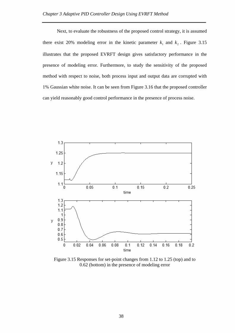
Next, to evaluate the robustness of the proposed control strategy, 10%
modeling error in the kinetic parameter and 20% modeling error in the
coefficient are considered. Figure 3.7 illustrates that the proposed EVRFT design
gives satisfactory performance in the presence of modeling error.
Ik
mM
Finally, to study the sensitivity of the proposed method with respect to noise,
both process input and output data are corrupted with 1% Gaussian white noise. It can
be seen from Figure 3.8 that the proposed controller can yield reasonably good control
performance in the presence of process noise.
Figure 3.7 Responses for +50% (top) and -50% (bottom) set-point changes by EVRFT design in the presence of modeling error
31

Chapter 3 Adaptive PID Controller Design Using EVRFT Method
Figure 3.8 Responses for +50% (top) and -50% (bottom) set-point changes by EVRFT design in the presence of process noise
Example 2 Considering the van de Vusse reactor with the following reaction
kinetic scheme: , , which is carried out in an isothermal CSTR.
The dynamics of the reactor are described by the following equations (Doyle et al.,
1995):
CBA →→ DA →
)(231 AAfAA
A CCVFCkCk
dtdC
−+−−= (3.23)
BBAB C
VFCkCk
dtdC
−−= 21 (3.24)
where the model parameters used are: , , 11 50 −= hk 1
2 100 −= hk )hL/(mol103 ⋅=k
,mol/L0.3=AC
BC
,
, and . The nominal operation condition is
, and . The concentration of component B, , is the
process output and the flow rate, , is the process input.
mol/L10=AfC
mol/L12.1=BC
L1=V
34=F L/h3.
F
32
Chapter 3 Adaptive PID Controller Design Using EVRFT Method
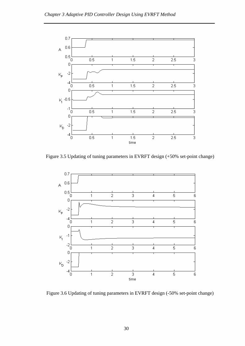
A salient feature of the above reactor is that the sign of its steady state gain
may change as the operation condition changes (see Figure 3.9). The database for
EVRFT design is generated by introducing random steps around the nominal value of
process input F as shown in Figure 3.10, where 1500 input/output data are used to
build the database. The process input and output are scaled by 31.34
31.34~ −=
uu and
12.112.1~ −
=yy respectively.
0 50 100 150 2000
0.2
0.4
0.6
0.8
1
1.2
1.4
F
C B
Figure 3.9 Steady-state curve of van de Vusse reactor
33

Chapter 3 Adaptive PID Controller Design Using EVRFT Method
Figure 3.10 Input-output data used for constructing the database (example 2)
To proceed with the EVRFT design, the tuning parameters specified are as
follows: the initial value of parameter A = 0.61, initial learning rate 5.8=η , weight
parameter used in the objective function Eq. (3.18) given by , the updating
parameters for learning rate
8.0=w
02.1=incl and 6.0=decl , and the number of data points
in the relevant dataset is set to 1200.
To evaluate the performance of the adaptive PID designed using EVRFT
method, two set-point changes from 1.12 to 1.25 and from 1.12 to 0.62 are conducted.
as illustrated in Figures 3.11 and 3.12. The corresponding updating of tuning
parameter A and PID parameters is shown in Figures 3.13 and 3.14, respectively.
Similar to Example 1, four PID controllers are designed using VRFT method
for the purpose of comparison. To match the performance of EVRFT design for the
set-point change to 0.62 as closely as possible, two PID controllers are obtained by
34

Chapter 3 Adaptive PID Controller Design Using EVRFT Method
VRFT design using the tuning parameter A = 0.65 for both reference model. Likewise,
to match the performance of EVRFT design for the set-point change to 1.25 as closely
as possible, another two PID controllers are obtained by VRFT design using tuning
parameters A = 0.37 and A = 0.35 for the first-order and second-order reference
models, respectively. As can be seen from Figure 3.11, the adaptive PID controller
designed using EVRFT method gives much faster response for set-point change from
1.12 to 1.25 than the two PID controllers that are deliberately designed to give
comparable performance to the EVRFT design for the set-point change from 1.12 to
0.62. Figure 3.12 shows similar observation for the other two PID controllers that are
designed to match the performance of EVRFT design for the set-point change to 1.25.
The tracking errors for various design methods are summarized in Table 3.4.
Table 3.4 Tracking errors obtained by various design methods
VRFT design using 1st-order model
VRFT design using 2nd-order model
EVRFT design
% Improvement (based on VRFT design using 2nd-order model)
Set-point change to
A=0.65 A=0.37 A=0.65 A=0.35 A=0.65 A=0.35 1.25 21054.3 −× 21021.2 −× 21051.3 −× 21093.1 −× 21055.1 −× 55.8% 19.7% 0.62 21008.5 −× 21079.5 −× 21092.4 −× 2 1025.8 −× 21078.4 −× 2.9% 42.1%
35

Chapter 3 Adaptive PID Controller Design Using EVRFT Method
Figure 3.11 Responses for set-point changes from 1.12 to 1.25 (top) and to 0.62 (bottom). Solid line: EVRFT; dotted line: VRFT using 2nd-order model (A = 0.65); dashed line: VRFT using1st-order model (A = 0.65)
Figure 3.12 Responses for set-point changes from 1.12 to 1.25 (top) and to
0.62 (bottom). Solid line: EVRFT; dotted line: VRF using 2nd-order model (A = 0.35); dashed line: VRFT using 1st-order model (A = 0.37)
36

Chapter 3 Adaptive PID Controller Design Using EVRFT Method
Figure 3.13 Updating of controller parameters in EVRFT design for
set-point change to 1.25
Figure 3.14 Updating of controller parameters in EVRFT design for
set-point change to 0.62
37
Chapter 3 Adaptive PID Controller Design Using EVRFT Method
Next, to evaluate the robustness of the proposed control strategy, it is assumed
there exist 20% modeling error in the kinetic parameter and . Figure 3.15
illustrates that the proposed EVRFT design gives satisfactory performance in the
presence of modeling error. Furthermore, to study the sensitivity of the proposed
method with respect to noise, both process input and output data are corrupted with
1% Gaussian white noise. It can be seen from Figure 3.16 that the proposed controller
can yield reasonably good control performance in the presence of process noise.
1k 2k
Figure 3.15 Responses for set-point changes from 1.12 to 1.25 (top) and to
0.62 (bottom) in the presence of modeling error
38

Chapter 3 Adaptive PID Controller Design Using EVRFT Method
Figure 3.16 Responses for set-point changes from 1.12 to 1.25 (top) and to
0.62 (bottom) in the presence of process noise
Finally, to further evaluate the performance of the proposed method, it is
assumed that there exists time delay in the output measurement of two sampling time.
In this case, most of tuning parameters for EVRFT design are identical to those used
for the case in the absence of time delay, except that the initial values of A and
learning rate η are changed as A = 0.53 and 5.3=η .
Figure 3.17 shows the resulting performances of ERFT design for the same
set-point changes described previously. The corresponding updating of controller
parameters is shown in Figures 3.18 and 3.19. For the purpose of comparison, a PID
controller designed using VRFT method with second-order reference model is
developed. The tuning parameter A = 0.63 is selected to obtain minimum tracking
error for the two set-point changes. The tracking errors for both EVRFT and VRFT
designs are summarized in Table 3.5. It can be seen from Figure 3.17 that the adaptive
39

Chapter 3 Adaptive PID Controller Design Using EVRFT Method
PID controller designed using EVRFT method gives better overall performance than
that obtained by the PID controller designed using VRFT with second-order reference
model.
Table 3.5 Tracking errors of EVRFT and VRFT designs for time delay case
Set-point change VRFT EVRFT % improvement 1.12 to 1.25 0.0382 0.0119 68.9% 1.12 to 0.62 0.0452 0.0413 8.6%
Figure 3.17 Responses for set-point changes from 1.12 to 1.25 (top) and to 0.62 (bottom) for time delay case. Solid line: EVRFT; dotted line: VRFT
40

Chapter 3 Adaptive PID Controller Design Using EVRFT Method
Figure 3.18 Updating of controller parameters in EVRFT design for set-point
change to 1.25 in the presence of time delay
Figure 3.19 Updating of controller parameters in EVRFT design for set-point
change to 0.62 in the presence of time delay
41
Chapter 3 Adaptive PID Controller Design Using EVRFT Method
42
3.5 Conclusion
In this chapter, an adaptive PID controller design method is proposed. The
proposed method makes use of the VRFT framework and achieves the adaptive nature
by updating the database, selecting a relevant dataset and most importantly, updating
the reference model parameter A at each sampling instance. Moreover, a second-order
reference model is employed for the VRFT design instead of the normally used first-
order reference model to achieve better performance. Simulation studies illustrate that
PID controllers designed using VRFT with a second-order reference model gives
better or comparable control performance than that obtained with a first-order
reference model. This justifies the use of second-order reference model in the
development of the proposed method. The simulation results also demonstrate that the
proposed EVRFT design gives marked improvement over the conventional VRFT
method.

Chapter 4
Adaptive Internal Model Controller
Design Using EVRFT Method
4.1 Introduction
Internal Model Control (IMC) is a powerful controller design strategy for the
open-loop stable dynamic systems (Morari and Zafiriou, 1989). A satisfactory
performance can be expected from IMC design as long as the process is operated in
the linear range around the point where the linear process model is obtained. However,
IMC controller may produce unsatisfactory or even unstable performance when it is
applied to nonlinear processes. To extend the IMC design to nonlinear processes,
various nonlinear and adaptive IMC schemes have been proposed in the literature as
reviewed in Chapter 2. However, all of the above nonlinear and adaptive IMC designs
bring in computationally demanding analytical or numerical methods and neural
networks in order to exhibit improved performance. This undermines the simplicity of
linear IMC design.
43

Chapter 4 Adaptive Internal Model Controller Design Using EVRFT Method
To circumvent the aforementioned drawback, the EVRFT method developed
in Chapter 3 is extended to the design of adaptive IMC controller in this chapter. In
the proposed method, the database for EVRFT design is updated at each sampling
instance by adding the current process data into the database and a relevant dataset is
selected according to the nearest neighbors’ criterion. In addition, the parameter of
reference model shall are updated for improved control performance. Finally, the
parameters of IMC controller are determined by solving an optimization problem
formulated in the VRFT design framework. Simulation results are presented to
illustrate the proposed design method and a comparison with conventional VRFT
design is made.
4.2 IMC Controller Design Using VRFT Method
The VRFT design using a second-order reference model discussed in Section
3.2 is applied here to design an IMC controller as shown in Figure 4.1. Without loss
of generality, a second-order ARX model is used to represent the IMC model:
( ) ( ) ( ) ( )121 121 −−+−+−= Nkukykyky βαα (4.1)
where ( )ky is the model output at the k-th sampling instance, is the
manipulated input at the (k-N-1)-th sampling instance, N is the process time delay,
and
( )1−− Nku
1α , 2α and 1β are IMC model parameters.
The corresponding transfer function of Eq. (4.1) is:
( ) 22
11
111
1~
−−
−−−
−−=
zzzzG
N
ααβ (4.2)
By using a first-order IMC filter, the IMC controller is obtained as )( 1−zQ
( ) 11
22
111
111
−
−−−
−−
⋅−−
=z
zzzQλλ
βαα (4.3)
44

Chapter 4 Adaptive Internal Model Controller Design Using EVRFT Method
r
Figure 4.1 Block diagram of IMC structure
where λ is the time constant of IMC filter. The corresponding feedback controller
( )θ;1−zC can be derived as
( ) ( )( ) ( ) ( ) 11
1
22
11
11
11
1111
~1; −−−
−−
−−
−−
−−−−
⋅−−
=−
= Nzzzz
zQzGzQzC
λλλ
βαα
θ (4.4)
In the VRFT design framework considered in this thesis, the reference model
( )1−zT is specified by the following second-order transfer function:
( )⎩⎨⎧
−−=+−=
+−+
== −−
−−−
−
−−
AAAAAAA
wherezAAz
zzzrzyzT
N
lnln1
21)()()( 2221
11
1
11
βαβα (4.5)
where A is the tuning parameter related to the speed of the response.
To design the IMC controller by the VRFT method, the virtual input ( )1~ −zu is
calculated by Eqs. (3.1), (3.2), (4.4) and (4.5) to obtain
( ) ( )( ) ( )( )[ ]( ) ( 1
1111
11221
1
22
111
112111~ −
−−−−−−
−−−−−−−−
+−−−+−+−
⋅−−−
= zyzzzz
zzzAAzzzzu NN
N
βαλλβα
βλαα )
)
(4.6)
Define ( 1~ −Φ z as follows:
( )[ ]( ) ( )11111 11)( −−−−−− +−−−=Φ zuzzzz N βαλλ (4.7)
The following equation can be obtained from Eqs. (4.6) and (4.7).
+ -
G
G~
Q+ -
y
yu
45

Chapter 4 Adaptive Internal Model Controller Design Using EVRFT Method
( )( ) ( ) ( 11
11221
1
22
111 2111
)(~ −−−
−−−−−−−− +−+−
⋅−−−
=Φ zyz
zzzAAzzzz N
Nβαβ
λαα ) (4.8)
Equation (4.7) can be rewritten as:
( ) ( ) ( ) ( ) ( ) ( ) ( )
( ) ( )211121
−−−−−−−−−−−−+=Φ
NkuNkukukukuk
λβλαλβαλβα
(4.9)
Equation (4.11) can be rewritten as:
( ) ( )kKk Ψ=Φ~ (4.10)
where
( ) ( ) ( ) ( )[ ]Tkkkk 321 ΨΨΨ=Ψ (4.11)
⎥⎦
⎤⎢⎣
⎡−−=
1
2
1
1
1
1βα
βα
βK (4.12)
with
( ) ( ) ( ) ( ) ( ) ( ) ( )[ ]11211 21 −−−−+++−++−=Ψ kykyNkyANkAyNkyk βαλ (4.13)
( ) ( ) ( ) ( ) ( ) ( ) ( )[ ]212121 22 −−−−−++−+−+−=Ψ kykyNkyANkAyNkyk βαλ (4.14)
( ) ( ) ( ) ( ) ( ) ( ) ( )[ ]3232211 23 −−−−−++−+−−+−=Ψ kykyNkyANkAyNkyk βαλ
(4.15)
Equation (3.3) is then expressed by
( ) ( ) ( ){ } 22
11
1min1min Ψ−Φ=Ψ−Φ= ∑=
Kn
kKkn
KJK
n
kK (4.16)
subject to the stability constraints imposed by the second-order IMC model:
⎥⎥⎥⎥⎥⎥
⎦
⎤
⎢⎢⎢⎢⎢⎢
⎣
⎡
>
⎥⎥⎥⎥⎥⎥⎥
⎦
⎤
⎢⎢⎢⎢⎢⎢⎢
⎣
⎡
−
−
⎥⎥⎥⎥⎥⎥
⎦
⎤
⎢⎢⎢⎢⎢⎢
⎣
⎡
−
−
⎥⎥⎥⎥⎥⎥
⎦
⎤
⎢⎢⎢⎢⎢⎢
⎣
⎡
<
⎥⎥⎥⎥⎥⎥⎥
⎦
⎤
⎢⎢⎢⎢⎢⎢⎢
⎣
⎡
−
−
⎥⎥⎥⎥⎥⎥
⎦
⎤
⎢⎢⎢⎢⎢⎢
⎣
⎡
−
−⇒
⎪⎩
⎪⎨
⎧
<>−+>−−
000001
001101
101111111
000001
001101
101111111
10101
1
2
1
1
1
1
2
1
1
1
2
21
21
βαβαβ
βαβαβ
ααααα
or
(4.17)
46
Chapter 4 Adaptive Internal Model Controller Design Using EVRFT Method
where
( ) ( ) ( )( ) ( ) ( )( ) ( ) ( )⎥
⎥⎥
⎦
⎤
⎢⎢⎢
⎣
⎡
ΨΨΨΨΨΨΨΨΨ
=Ψnnn
333
222
111
212121
L
L
L
(4.18)
( )[ nΦΦ=Φ L1 ( )] (4.19)
Consequently, IMC model parameters are obtained by solving the constrained
least square problem as stated in Eq. (4.16). It is evident that this solution not only
depends on the database for VRFT design but also the design parameter A in the
reference model.
The control action taken by the IMC controller is calculated by:
( ) ( ) ( ) ( ) ( )[ ]2111 21 −−−−−
+−= kekekekuku ααβλλ (4.20)
where ( ) ( ) ( ) ( )kykykrke +−= and ( )kr is the set-point at k-th sampling instance.
4.3 Enhanced VRFT Design Method
Similar to Section 3.3, when the EVRFT method is used to design an adaptive
IMC controller, tuning parameter A in the reference model is updated at each
sampling instance as it has a direct impact on the IMC model parameters calculated
using the VRFT method.
The objective of adjusting reference model parameter A is to minimize the
following quadratic function:
( ) ( ) ( ) ( )[ ] ( ) ( )[{ }222 11ˆ11
21
−−++−+−= kukuwkykrwkJ ]
]
(4.21)
where is a weight parameter and [ 1,0∈w ( )1ˆ +ky is the predicted output using the
reference model at the (k+1)-th sampling instance which can be calculated by:
( ) ( ) ( ) ( ) ( )1121ˆ 2 −−+−+−−=+ NkrNkrkyAkAyky βα (4.22)
47
Chapter 4 Adaptive Internal Model Controller Design Using EVRFT Method
By the steepest descent method, the updating algorithm is derived as:
( ) ( ) ( ) ( )( )kA
kJkkAkA
∂∂
−=+ 21 η (4.23)
where ( )kη is the learning rate.
The following summarizes the computational algorithm for the proposed
EVRFT design of adaptive IMC controller:
Step 1 The process Input (u(k)) and output (y(k)) identification data that characterize
the dynamics of nonlinear system are assumed to be available and the off-line
database for EVRFT design is constructed as ( ) niix ~1= ;
Step 2 At the k-th sampling instance, based on the current database for EVRFT
design, the relevant dataset is selected according to Eq. (2.4) and then the IMC
model parameters are calculated by solving the minimization problem given
by Eq. (4.16) subjected to the constraint Eq. (4.17). The manipulated variable
is obtained by Eq. (4.20). ( )ku
Step 3 The database for VRFT design is augmented by appending the current process
data ( )ky and ; while the tuning parameter A is updated using Eq. (4.23). ( )ku
Step 4 Set and go to Step 2. 1+= kk
4.4 Examples
Example 1 Considering the continuous polymerization reaction studied in
Chapter 3 with model parameters and steady-state operating condition given in Table
3.1 and 3.2.
To apply the EVRFT method to design the adaptive IMC controller, the
identical off-line process data used in Chapter 3 are employed. The tuning parameters
specified for EVRFT design are as follows: the IMC filter parameter 7.0=λ , the
48
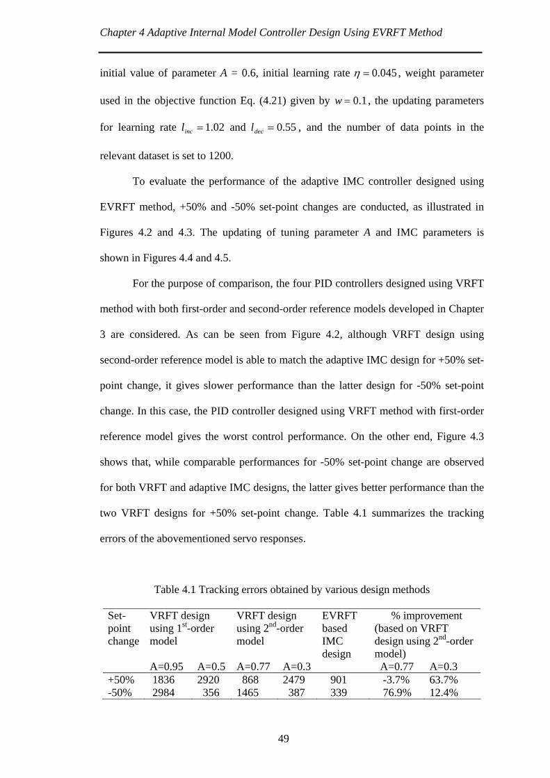
Chapter 4 Adaptive Internal Model Controller Design Using EVRFT Method
initial value of parameter A = 0.6, initial learning rate 045.0=η , weight parameter
used in the objective function Eq. (4.21) given by 1.0=w , the updating parameters
for learning rate and 02.1=incl 55.0=decl , and the number of data points in the
relevant dataset is set to 1200.
To evaluate the performance of the adaptive IMC controller designed using
EVRFT method, +50% and -50% set-point changes are conducted, as illustrated in
Figures 4.2 and 4.3. The updating of tuning parameter A and IMC parameters is
shown in Figures 4.4 and 4.5.
For the purpose of comparison, the four PID controllers designed using VRFT
method with both first-order and second-order reference models developed in Chapter
3 are considered. As can be seen from Figure 4.2, although VRFT design using
second-order reference model is able to match the adaptive IMC design for +50% set-
point change, it gives slower performance than the latter design for -50% set-point
change. In this case, the PID controller designed using VRFT method with first-order
reference model gives the worst control performance. On the other end, Figure 4.3
shows that, while comparable performances for -50% set-point change are observed
for both VRFT and adaptive IMC designs, the latter gives better performance than the
two VRFT designs for +50% set-point change. Table 4.1 summarizes the tracking
errors of the abovementioned servo responses.
Table 4.1 Tracking errors obtained by various design methods
VRFT design using 1st-order model
VRFT design using 2nd-order model
% improvement (based on VRFT design using 2nd-order model)
Set- point change
A=0.95 A=0.5 A=0.77 A=0.3
EVRFT based IMC design
A=0.77 A=0.3 +50% 1836 2920 868 2479 901 -3.7% 63.7% -50% 2984 356 1465 387 339 76.9% 12.4%
49

Chapter 4 Adaptive Internal Model Controller Design Using EVRFT Method
Figure 4.2 Responses for +50% (top) and -50% (bottom) set-point changes. Solid line: EVRFT; dotted line: VRFT using 2nd-order model (A=0.77);
dashed line: VRFT using 1st-order model (A=0.95)
Figure 4.3 Responses for +50% (top) and -50% (bottom) set-point changes. Solid line: EVRFT; dotted line: VRFT using 2nd-order model (A = 0.3);
dashed line: VRFT using 1st-order model (A = 0.5)
50
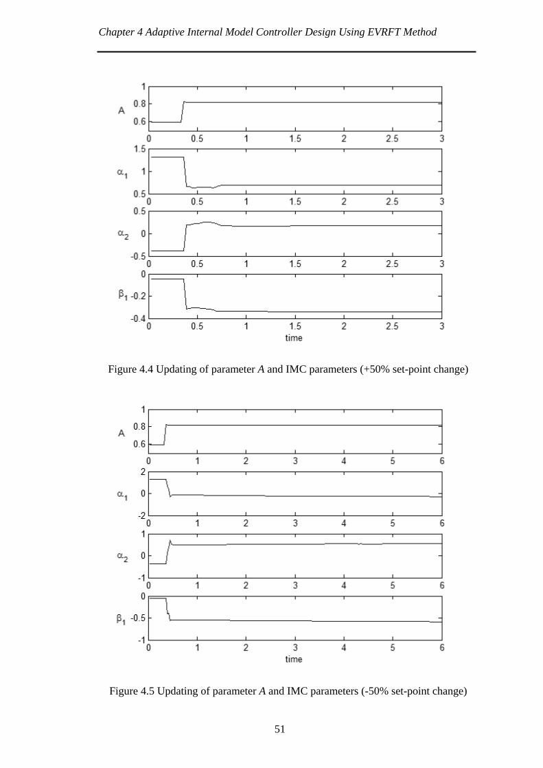
Chapter 4 Adaptive Internal Model Controller Design Using EVRFT Method
Figure 4.4 Updating of parameter A and IMC parameters (+50% set-point change)
Figure 4.5 Updating of parameter A and IMC parameters (-50% set-point change)
51
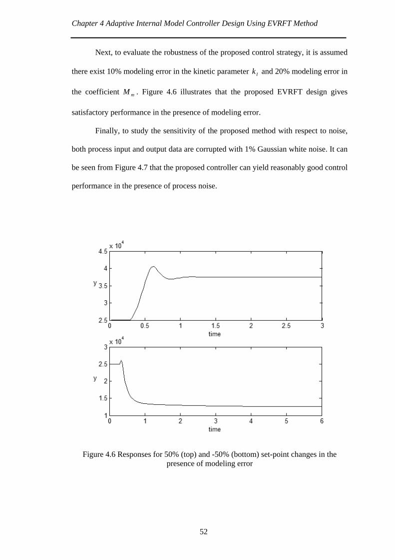
Chapter 4 Adaptive Internal Model Controller Design Using EVRFT Method
Next, to evaluate the robustness of the proposed control strategy, it is assumed
there exist 10% modeling error in the kinetic parameter and 20% modeling error in
the coefficient . Figure 4.6 illustrates that the proposed EVRFT design gives
satisfactory performance in the presence of modeling error.
Ik
mM
Finally, to study the sensitivity of the proposed method with respect to noise,
both process input and output data are corrupted with 1% Gaussian white noise. It can
be seen from Figure 4.7 that the proposed controller can yield reasonably good control
performance in the presence of process noise.
Figure 4.6 Responses for 50% (top) and -50% (bottom) set-point changes in the presence of modeling error
52
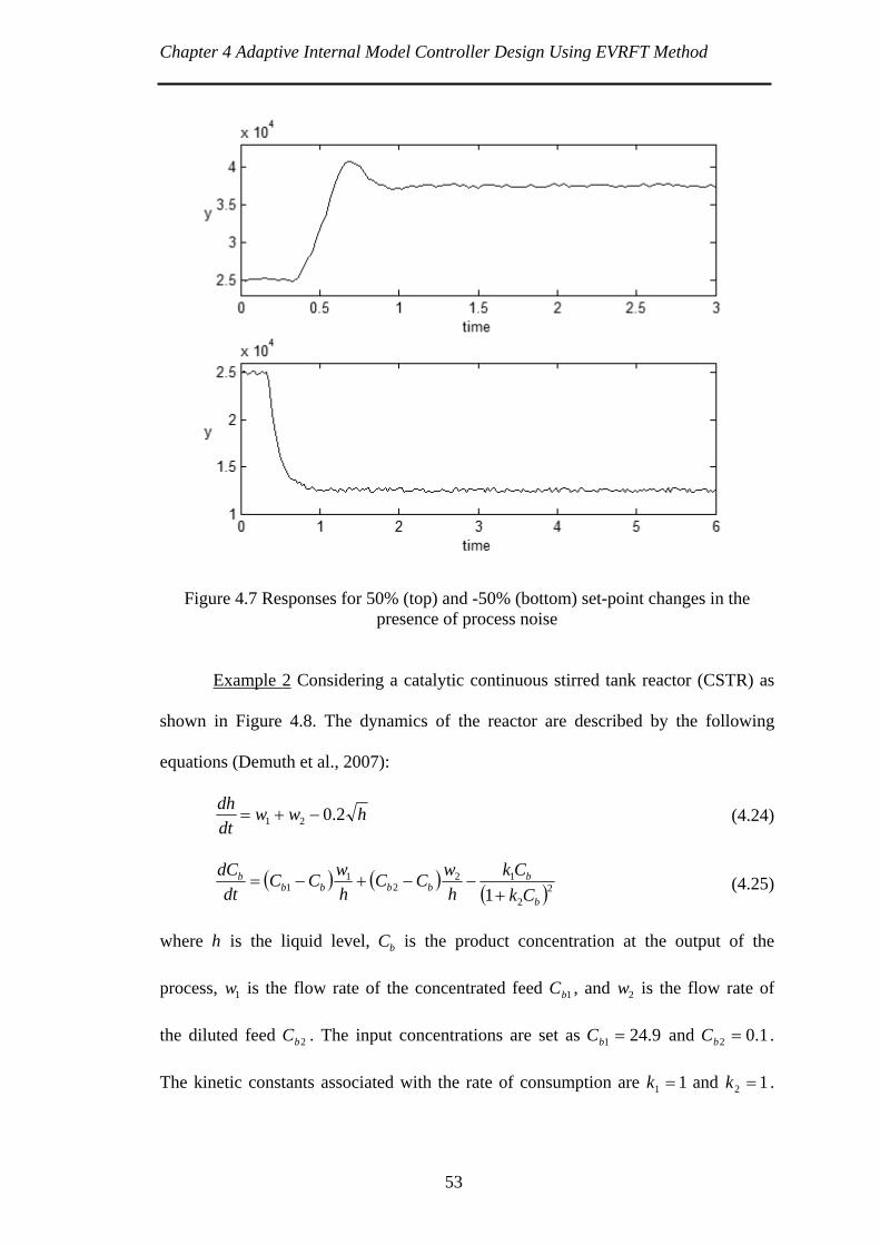
Chapter 4 Adaptive Internal Model Controller Design Using EVRFT Method
Figure 4.7 Responses for 50% (top) and -50% (bottom) set-point changes in the presence of process noise
Example 2 Considering a catalytic continuous stirred tank reactor (CSTR) as
shown in Figure 4.8. The dynamics of the reactor are described by the following
equations (Demuth et al., 2007):
hwwdtdh 2.021 −+= (4.24)
( ) ( )( )22
122
11 1 b
bbbbb
b
CkCk
hwCC
hwCC
dtdC
+−−+−= (4.25)
where is the liquid level, is the product concentration at the output of the
process, is the flow rate of the concentrated feed , and is the flow rate of
the diluted feed . The input concentrations are set as
h bC
1w 1bC 2w
242bC 9.1 =bC and 1.02 =bC
12
.
The kinetic constants associated with the rate of consumption are and 1=1k =k .
53

Chapter 4 Adaptive Internal Model Controller Design Using EVRFT Method
The product concentration, , is the process output and the flow rate, , is the
process input. To simplify the demonstration, the flow rate of the diluted feed is set as
. The nominal operating condition of the reactor are ,
and .
bC 1w
20=( ) 1.02 =tw
25.12=h
5839.bC
6.01 =w
Figure 4.8 The catalytic continuous stirred tank reactor
A salient feature of the above reactor is that the sign of its steady state gain
may change as the operation condition changes (see Figure 4.9). The database for
EVRFT design is generated by introducing uniformly random steps with distribution
of and the switching probability of 0.2 at every sampling time to the process
input . With a sampling time of 0.2, 1500 input/output data as shown in Figure 4.10
are collected to build the database. The process input and output are scaled by
]2.1,0[
1w
6.06.0~ −
=uu and
20.583920.5839~ −
=yy respectively.
54
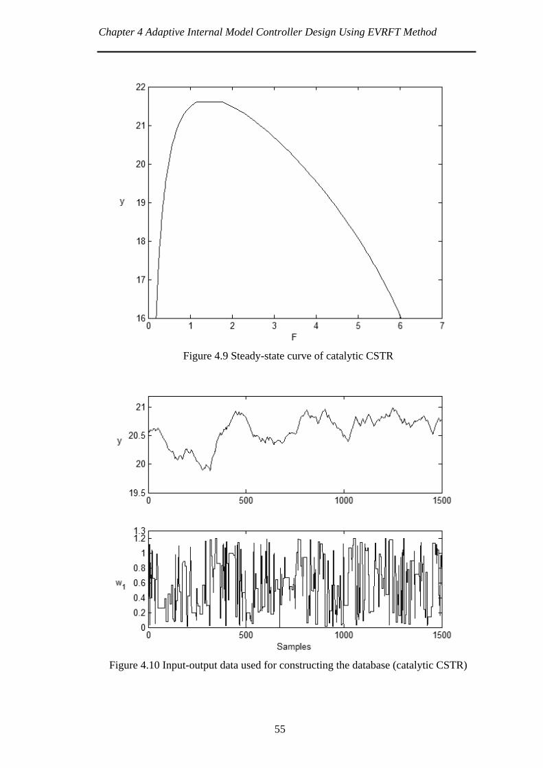
Chapter 4 Adaptive Internal Model Controller Design Using EVRFT Method
Figure 4.9 Steady-state curve of catalytic CSTR
Figure 4.10 Input-output data used for constructing the database (catalytic CSTR)
55

Chapter 4 Adaptive Internal Model Controller Design Using EVRFT Method
To proceed with the EVRFT design of adaptive IMC controller, the tuning
parameters specified are as follows: the IMC filter parameter is fixed as 01.0=λ , the
initial value of parameter A = 0.4, initial learning rate , weight parameter
used in the objective function Eq. (3.18) given by
3105.2 −×=η
7.0=w , the updating parameters
for learning rate and 02.1=incl 55.0=decl , and the number of data points in the
relevant dataset is set to 1200.
To evaluate the performance of the adaptive IMC designed using EVRFT
method, two respective set-point changes from the nominal operating condition to
21.5 and to 19.5 are conducted, as illustrated in Figure 4.11. The corresponding
updating of tuning parameter A and IMC parameters in the above servo responses is
shown in Figures 4.12 and 4.13.
For the purpose of comparison, PID controllers designed using the VRFT
method with both first-order and second-order reference models are developed. The
tuning parameter A = 0.96 is selected for the first-order case and A = 0.74 is selected
for the second order case to achieve the minimum tracking errors for the two set-point
changes. It is evident from Figure 4.11 that the adaptive IMC controller designed
using EVRFT method gives faster response for both set-point changes than the two
PID controllers designed by VRFT method. Moreover, the PID controller designed
using second-order reference model shows better performance than that with a first-
order reference model. The tracking errors for all methods are summarized in Table
4.2.
Table 4.2 Tracking errors obtained by various design methods
Set-point change to
VRFT design using 1st-order model
VRFT design using 2nd-order model
EVRFT based IMC design
% improvement (based on VRFT design using 2nd-order model)
21.5 0.1385 0.0977 0.0754 22.8% 19.5 0.2270 0.1753 0.1384 21.1%
56

Chapter 4 Adaptive Internal Model Controller Design Using EVRFT Method
Figure 4.11 Closed-loop responses for set-point changes to 21.5 (top) and to 19.5 (bottom). Solid line: EVRFT; dotted line: VRFT using 2nd-order model; dashed line:
VRFT using 1st-order model
Next, to evaluate the robustness of the proposed control strategy, 10%
modeling errors in the kinetic parameter and are considered. Figure 4.14
illustrates that the proposed EVRFT design gives satisfactory performance in the
presence of modeling error. Furthermore, to study the sensitivity of the proposed
method with respect to noise, both process input and output data are corrupted with
1% Gaussian white noise. It can be seen from Figure 4.15 that the proposed controller
can yield reasonably good control performance in the presence of process noise.
1k 2k
Finally, to further evaluate the performance of the proposed method, it is
assumed that there exists time delay in the output measurement of five sampling time.
In this case, most of tuning parameters for EVRFT design are identical to those used
for the case in the absence of time delay, except that the initial values of A and
57
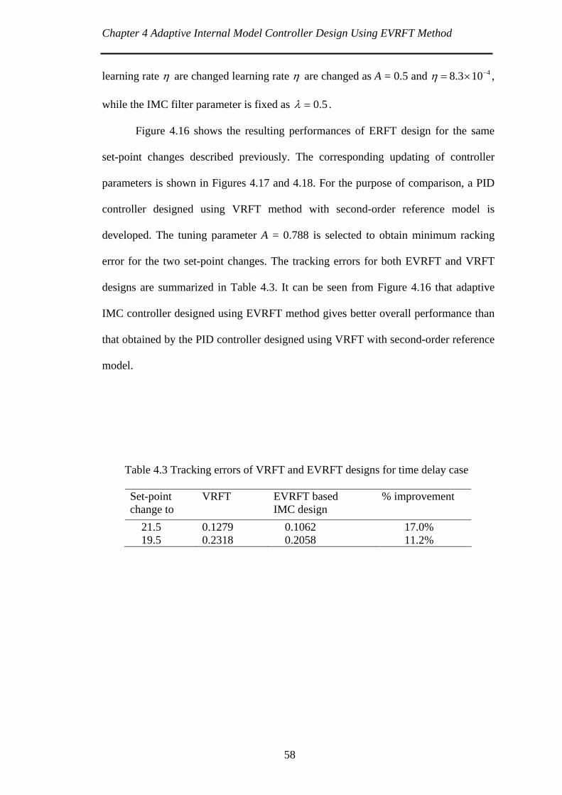
Chapter 4 Adaptive Internal Model Controller Design Using EVRFT Method
learning rate η are changed learning rate η are changed as A = 0.5 and ,
while the IMC filter parameter is fixed as
4103.8 −×=η
5.0=λ .
Figure 4.16 shows the resulting performances of ERFT design for the same
set-point changes described previously. The corresponding updating of controller
parameters is shown in Figures 4.17 and 4.18. For the purpose of comparison, a PID
controller designed using VRFT method with second-order reference model is
developed. The tuning parameter A = 0.788 is selected to obtain minimum racking
error for the two set-point changes. The tracking errors for both EVRFT and VRFT
designs are summarized in Table 4.3. It can be seen from Figure 4.16 that adaptive
IMC controller designed using EVRFT method gives better overall performance than
that obtained by the PID controller designed using VRFT with second-order reference
model.
Table 4.3 Tracking errors of VRFT and EVRFT designs for time delay case
Set-point change to
VRFT EVRFT based IMC design
% improvement
21.5 0.1279 0.1062 17.0% 19.5 0.2318 0.2058 11.2%
58

Chapter 4 Adaptive Internal Model Controller Design Using EVRFT Method
Figure 4.12 Updating of parameter A and IMC parameters for set-point change to 21.5
Figure 4.13 Updating of parameter A and IMC parameters for set-point change to 19.5
59
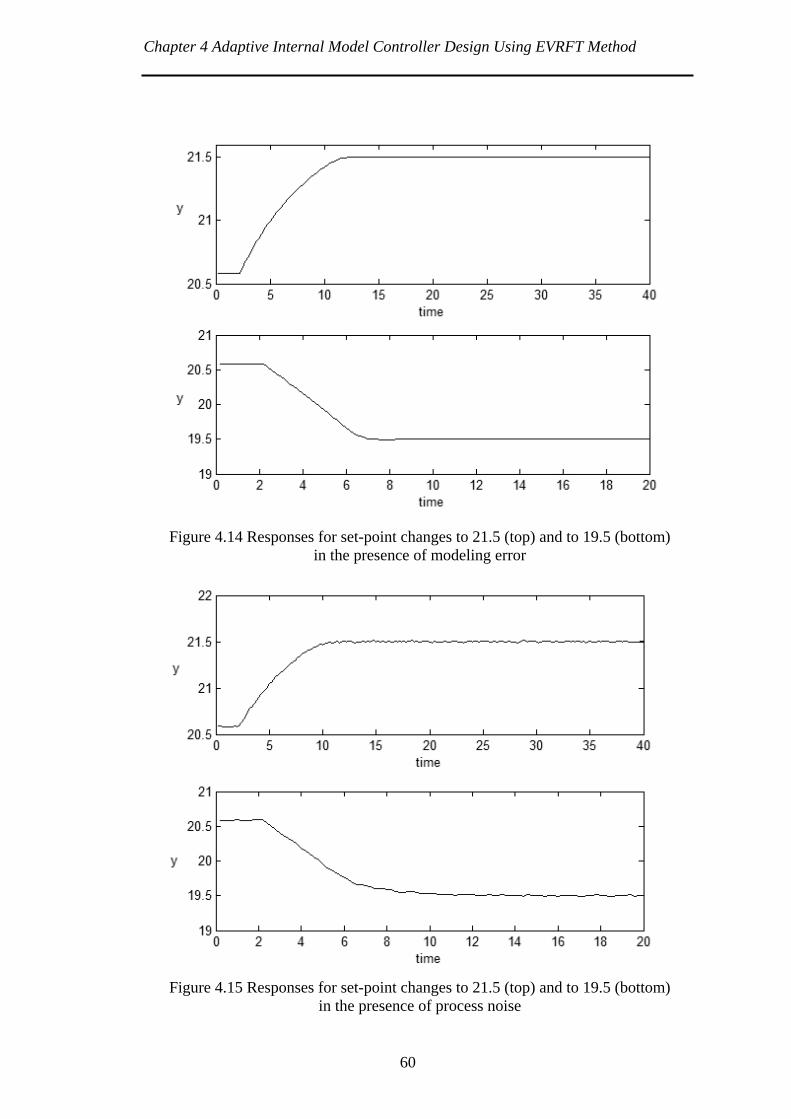
Chapter 4 Adaptive Internal Model Controller Design Using EVRFT Method
Figure 4.14 Responses for set-point changes to 21.5 (top) and to 19.5 (bottom)
in the presence of modeling error
Figure 4.15 Responses for set-point changes to 21.5 (top) and to 19.5 (bottom)
in the presence of process noise
60

Chapter 4 Adaptive Internal Model Controller Design Using EVRFT Method
Figure 4.16 Responses for set-point changes to 21.5 (top) and to 19.5 (bottom) in the presence of time delay. Solid line: EVRFT; dotted line: VRFT
Figure 4.17 Updating of parameter A and IMC parameters set-point change
to 21.5 in the presence of time delay
61

Chapter 4 Adaptive Internal Model Controller Design Using EVRFT Method
62
Figure 4.18 Updating of parameter A and IMC parameters for set-point change
to 19.5 in the presence of time delay
4.5 Conclusion
In this chapter, an adaptive IMC design method is proposed. The proposed
method makes use of the VRFT design and achieves the adaptive nature by updating
the database, selecting a relevant dataset and most importantly, updating the reference
model parameter A at each sampling instance. Moreover, a second-order reference
model is employed for the VRFT design instead of the commonly used first-order
reference model to achieve better control performance. The simulation results
demonstrate that the proposed method gives improved performance over the
conventional VRFT design.
Chapter 5
Conclusions and Further Work
5.1 Conclusions
In this thesis, the Enhanced Virtual Reference Feedback Tuning (EVRT)
method is proposed and two adaptive controllers, namely adaptive PID controller and
adaptive IMC controller, are developed using the EVRFT method. This method make
use of information extracted from the process input and output database to obtain
controller parameters at each sampling instance. The adaptive nature of this method is
achieved by: (i) update the database by adding the current process data into the
database; (ii) using the relevant dataset selected from the current database based on k-
nearest neighborhood criterion; (iii) update the parameters in the reference model.
Moreover, a second-order reference model is used in both designs instead of the first-
order reference model normally used in the literature.
Simulation results are presented for both nominal cases and cases in the
presence of modeling error and process noise. Both adaptive PID and IMC designs by
the proposed EVRFT design are observed give faster and less oscillatory responses
63

Chapter 5 Conclusions and Further Work
64
than the PID controller designed using VRFT method. In summary, the EVRFT
method is a useful strategy for adaptive controller design for nonlinear processes.
5.2 Suggestions for Further Work
There are few open questions that need to be further studied. Some possible
topics for future research are listed below.
The present study focuses on the servo performance in the controller design. It
is thus of practical importance to extend the EVRFT design to address disturbance
rejection performance. Furthermore, the EVRFT method may be applied to more
complicated control systems such as cascade control. Finally, the application of the
EVRFT method to the multivariable systems may also be an interesting topic.

Appendix A
Derivation of the 2nd-order Reference Model
Consider the following second-order transfer function with a zero-order hold:
( )tsN
ts
ess
e Δ−Δ−
⋅+
⋅−
2111
λ (A.1)
where is the process time delay, tN Δ⋅ tΔ is the sampling period and λ is the time
constant. Applying Z-transform of Eq. (A.1) obtains
( )( )
( )
( ) ( ) ⎥⎥⎦⎤
⎢⎢⎣
⎡
−
Δ−
−−
−−=
⎭⎬⎫
⎩⎨⎧
+−
+−⋅−=
⎭⎬⎫
⎩⎨⎧
⋅+
⋅−
−
−
−−−−
−−Δ−Δ−
21
1
111
21
2
111
111
1111
111
AztAz
Azzzz
sssZzze
sseZ
N
NtsNts
λ
λλ
λλ
λ
(A.2)
where λt
eAΔ−
= and hence λtA Δ
−=ln . Equation (A.2) can thus be simplified as:
( ) ( )[ ]( )
( )221
11
21
121
211lnln1
−−
−−−
−
−−−
+−+
=−
−−++−⋅
zAAzzz
AzzAAAAAAAzz
NN βα
(A.3)
where AAA ln1 +−=α and . AAAA ln2 −−=β
65

References
Alpbaz, M., Hapoglu, H., Ozkan, G., and Altuntas, S. (2006). Application of
selftuning PID control to a reactor of limestone slurry titrated with sulfuric acid.
Chemical Engineering Journal, 116, 19-24.
Altinten, A., Erdogan, S., Alioglu, F., Hapoglu, H., and Alpbaz, M. (2004).
Application of adaptive PID control with genetic algorithm to a polymerization
reactor. Chemical Engineering Communications, 191, 1158-1172.
Andrasik, A., Meszaros, A., and de Azevedo, S. F. (2004). On-line tuning of a neural
PID controller based on plant hybrid modeling. Computers and Chemical Engineering,
28, 1499-1590.
Aoyama, A., Doyle, F. J. III, and Venkatasubramanian, V. (1995). Control-affine
fuzzy neural network approach for nonlinear process control. Journal of Process
Control, 5, 375-386.
Åström, K. J. (1983). Theory and application of adaptive control – A survey.
Automatica, 19, 471-486.
Åström, K. J. and Wittenmark, B. (1995). Adaptive control, 2nd Edition. Addison-
Welsey.
66

References
Bhat, N. and Mcavoy, T. J. (1990). Use neural nets for dynamic modeling and control
of chemical process systems. Computer and Chemical Engineer, 14, 573-583.
Bisowarno, B. H., Tian, Y. C., and Tade, M. O. (2004). Adaptive control of an ETBE
reactive distillation column. Journal of Chemical Engineering of Japan, 37, 210-216.
Böling, J. M., Seborg, D. E. and Hespanha, J. P. (2007). Multi-model adaptive control
of a simulated pH neutralization process. Control Engineering Practice, 15, 663-672.
te Braake, H. A. B., van Can, E. J. L., Scherpen, J. M. A., and Verbruggen, H. B.
(1998). Control of nonlinear chemical processes using neural models and feedback
linearization. Computers and Chemical Engineering, 22, 1113-1127.
Calvet, J. P. and Arkun, Y. (1988). Feedforward and feedback linearization of
nonlinear systems and its implementation using internal model control (IMC).
Industrial and Engineering Chemistry Research, 27, 1822-1831.
Campi, M. C., Lecchini, A., and Savaresi, S. M. (2000). Virtual reference feedback
tuning (VRFT): a new direct approach to the design of feedback controllers.
Proceedings of the 39th IEEE Conference on Decision and Control, 623-629.
Campi, M. C., Lecchini, A., and Savaresi, S. M. (2002). Virtual reference feedback
tuning: a direct method for the design of feedback controllers. Automatica, 38, 1337-
1346.
Chen, J. and Huang, T. (2004). Applying neural networks to on-line updated PID
controllers for nonlinear process control. Journal of Process Control, 14, 211-230.
Cheng, C. and Chiu, M. S. (2007). Adaptive IMC controller design for nonlinear
process control. Chemical Engineering Research & Design, 85, 234-244.
Demuth H., Beale M. and Hagan M. (2007), Neural Network Toolbox 5, The
Mathworks, Natick, MA (2007)
67
References
Doyle, F. J., Ogunnaike, B. A., and Pearson, R. K. (1995). Nonlinear model-based
control using second-order volterra models. Automatica, 31, 697-714.
Economou, C. G., Morari, M., and Palsson, B. O. (1986). Internal model control. 5.
Extention to nonlinear systems. Ind. Eng. Chem. Process Des. Dev. 25, 403-411.
Ge, S. S., Hang, C. C., Lee, T. H., and Zhang, T. (2002). Stable adaptive neural
network control. Kluwer Academic, Boston.
Gracia, C. E. and Morari, M. (1982). Internal model control – 1. a unifying review
and some new results. Ind. Eng. Chem. Process Des. & Dev., 21, 308-323.
Guardabassi, G. O., and Savaresi, S. M. (1997). Approximate feedback linearization
of discrete-time non-linear systems using virtual input direct design. Systems and
Control Letters, 32, 63-74.
Guardabassi, G. O., and Savaresi, S. M. (2000). Virtual reference direct design
method: an off-line approach to data-based control system design. IEEE Transactions
on Automatic Control, 45, 954-959.
Harris, K. R. and Palazoglu, A. (1998). Studies on the analysis of nonlinear process
via functional expansions-III: Controller design. Chemical Engineering Science, 53,
4005-4022.
Henson, M. A. and Seborg, D.E. (1991a). Critique of exact linearization strategies for
process control. Journal of Process Control, 1, 122-139.
Henson, M. A. and Seborg, D. E. (1991b). An internal model control strategy for
nonlinear systems. AIChE Journal, 37, 1065-1078.
Hernandez, E. and Arkun, Y. (1992). Study of the control-relevant properties of
backpropagation neural network models of nonlinear dynamical systems. Computers
and Chemical Engineering, 16, 227-240.
68

References
Hjalmarsson, H., Gunnarsson, S., and Gevers, M. (1994). A convergent iterative
restricted complexity control design scheme. Proceedings of the 33rd IEEE
Conference on Decision and Control, 1735-1740.
Hjalmarsson, H., Gevers, M., Gunnarsson, S., and Lequin, O. (1998). Iterative
feedback tuning: theory and applications. IEEE Control Systems Magazine,18, 26-41.
Ho, H. L., Rad, A. B., Chan, C. C., and Wong, Y. K. (1999). Comparative studies of
three adaptive controllers. ISA Transactions, 38, 43-53.
Hunt, K. J. and Sbarbaro, D. (1991). Neural networks for nonlinear internal model
control. IEE Proceedings-D, 138, 431-438.
Jin, L., Nikiforuk, P. N., and Gupta, M. M. (1994). Adaptive control of discrete-time
nonlinear systems using recurrent neural networks. IEE Proceedings – Control
Theory and Application, 141, 169-176.
Kalmukale, A. G., Chiu, M. S. and Wang, Q. G. (2007). Partitioned model-based IMC
design using JITL modeling technique. Journal of Process Control, 17, 757-769.
Kansha, Y., Hashimoto, Y., and Chiu, M. S. (2008). New results on VRFT design of
PID controller. Chemical Engineering Research & Design, 86, 925-931
Lewis, F. L., Yesildireck, A., and Liu, K. (1996). Multilayer neural-net robot
controller with guaranteed tracking performance. IEEE Transactions on Neural
Networks, 7, 388-389.
Linkens, D. A. and Nyongesa, H. O. (1996). Learning systems in intelligent control:
an appraisal of fuzzy, neural and genetic algorithm control applications. IEE
Proceeding – Control Theory and Applications, 143, 367-386.
Maksumov, A., Mulder, D. J., Harris K. R., and Palazoglu, A. (2002). Experimental
application of partitioned model-based control to PH neutralization. Industrial and
Engineering Chemistry Research, 41, 744-750.
69

References
Maner, B. R., Dolye, F. J. III, Ogunnaike, B. A., and Pearson, P. K. (1996). Nonlinear
model predictive control of a simulated multivariable polymerization reactor using
second-order Volterra models. Automatica, 32, 1285-1301.
Morari, M. and Zafiriou, E. (1989). Robust Process Control. Prentice Hall,
Englewood Cliffs, NJ.
Nahas, E. P., Henson, M. A., and Seborg, D. E. (1992). Nonlinear internal model
control strategy for neural network models. Computers and Chemical Engineering, 16,
1039-1057.
Nakamoto, M. (2005). An application of the virtual reference feedback tuning method
for a multivariable process control. Transactions of the Society of Instrument and
Control Engineers, 41.
Narendra, K. S. and Parthasarathy, K. (1990). Identification and control of dynamical
systems using neural networks. IEEE Transactions on Neural Networks, 1, 4-27.
Pan, T., Li, S., and Cai, W. J. (2007). Lazy learning-based online identification and
adaptive PID control: a case study for CSTR process. Industrial and Engineering
Chemistry Research, 46, 472-480.
Pérez, J. A., Ocaña, J. L., Molpeceres, C., Morales, M. and Blasco, M. (2009).
Adaptive neural network control system for laser surface heat treatments.
International Journal of Advanced Manufacturing Technology, 41, 513-518.
Polycarpou, M. M. (1996). Stable adaptive neural control scheme for nonlinear
systems. IEEE Transaction on Neural Networks, 3, 837-863.
Riverol, C., and Napolitano, V. (2000). Use of neural networks as a tuning method for
an adaptive PID application in a heat exchanger. Chemical Engineering Research and
Design, 78, 1115-1119.
70

References
71
Savaresi, S. M., and Guardabassi, G. O. (1998). Approximate I/O feedback
linearization of discrete-time non-linear systems via virtual input direct design.
Automatica, 34, 715-722.
Seborg, D. E., Edgar, T. F., and Shah, S. L. (1986). Adaptive control strategies for
process control: a survey. AIChE Journal, 32, 881-913.
Shahrokhi, M., and Baghmisheh, G. R. (2005). Modeling, simulation and control of a
methanol synthesis fixed-bed reactor. Chemical Engineering Science, 60, 4275-4286.
Shaw, A. M., Dolye, F. J. III, and Schwaber, J. S. (1997). Dynamic neural network
approach to nonlinear process modeling. Computers and Chemical Engineering, 21,
371-385.
Spall, J. C., and Cristion, J. A. (1998). Model-free control of nonlinear stochastic
systems with discrete-time measurements. IEEE Transactions on Automatic Control,
43, 1198-1210.
Stephanopoulos, G. and Han, C. (1996). Intelligent systems in process engineering: a
review. Computers and Chemical Engineering, 20, 743-791.
Xiong, Q., and Jutan, A. (2002). Grey-box modeling and control of chemical
processes. Chemical Engineering Science, 57, 1027-1039.
Yamamoto, T., and Shah, S. L. (2004). Design and experimental evaluation of a
multivariable self-tuning PID controller. IEE Proceeding - Control Theory and
Applications, 151, 645-652.
Yu, D. L., Chang, T. K. and Yu D. W. (2007). A stable self-learning PID control for
multivariable time varying systems. Control Engineering Practice, 15, 1577-1587.