adaptive control: an introduction - unibo.it · pdf filein an adaptive control system, two...

Adaptive Control:

an introduction

Claudio Melchiorri

Dipartimento di Ingegneria dell’Energia Elettrica e dell’Informazione (DEI)

Universita di Bologna

email: [email protected]

C. Melchiorri (DEI) Adaptive Control: an introduction 1 / 68

Summary

1 Introduction

2 Least squares estimationGeometric interpretationRecursive formulationTime-varying parameters

3 Application to linear dynamic systemsSome implementation aspects

4 Design of ST controllers by poles/zeros assignment


Introduction

Adaptive regulators

An adaptive regulator is able to modify automatically its own behaviour in orderto react to variations in the process dynamics and/or to external disturbances.The goal is to guarantee in any case the achievement of pre-assigned constraints(design specifications) on the controlled system. Adaptive control schemes allowto:

estimate online the value of the plant parameters (not known ortime-varying),

adapt the control parameters on the basis of this estimation.

In an adaptive control system, two feedback loops may be defined:

the standard control feedback loop based on the output signal and acting onthe input of the process (higher frequency)

a loop taking into account the design specifications, acting on the parametersof the controller (lower frequency).


Introduction

Adaptive regulators

Two general control schemes have been defined in the literature:

Model Reference Adaptive System (MRAS)

Self Tuning Regulator (STR)

In MRAS schemes, the adaptation law affects the control parameters in order tokeep y , the output of the process, as similar as possible to ym, the output of areference model.

Regulator Process

Adaptation

Model

parameters

✲ ✲ ✲✲

✛❄

❄

✲

✲

v u y

ym


Introduction

Adaptive regulators

STR (Self Tuning Regulator) schemes:

- Indirect methods: the adaptation algorithm estimates the parameters of the plant,and then a synthesis procedure is used for the control algorithm

- Direct methods: the parameters of the control law are directly modified by theadaptation algorithm (as for MRAS)

Indirect STR scheme

Regulator Process

EstimatorSynthesis

✲ ✲ ✲✲

✛✲

v u y❄

❄estimated plant parameters

Direct (implicit) STR scheme

Regulator Process

Estimator

✲✲✲✲

✛✲

❄ yv u

control parameters


Introduction

Adaptive regulators

Adaptive control schemes:

- Certainty equivalence property: the parameters estimated online areconsidered, for the control synthesis, equal to the true ones (not known)

- Adaptive control schemes are non linear dynamic systems with time-varyingparameters

Only a specific class of adaptive controllers is considered here: STR with leastsquares estimation and synthesis based on pole/zero placement.


Introduction

Adaptive regulators - An example

Let us consider the control of the variable φ = ω (angular velocity about thevertical axis).

Define:

τm: input torque applied by the motor (joint φ)

τa: friction torque

Jl : load inertia seen at the motor side, Jl = Jl (M, θ)

Balance of torques at joint axis (if M is constant) and variation ofangular momentum:

∑

τi =ddt

(

Jφ)

= Jφ+ d Jdθ

θφ, if θ = 0 =⇒ Jφ = τa + τm


Introduction


❜��

��

✈Mθ

a

φ

✒

The inertia J seen at the motor is given by

J = Jm +Jlk2r

whereJl = M a2 sin2(θ)

and kr is the reduction ratio of the motor.


Introduction


Assuming θ constant and τa = 0, then Jφ = τm, with τm = kmi

PI Motor Joint ✲✲ ✲✲✲ωr ω = φi τm

With a PI controller, the motor current i is computed as

i = k

[

(ωr − ω) +1

Ti

∫ t

0

(ωr − ω)dt

]

Therefore Jd2 ω

dt2+ kmk

d ω

dt+

kmk

Ti

ω = kmkd ωr

dt+

kmk

Ti

ωr

that isω(s)

ωr (s)= G0(s) =

2δ0ω0s + ω20

s2 + 2δ0ω0s + ω20

with

k =2δ0ω0J

km

Ti =2δ0ω0


Introduction


If the PI parameters k ,Ti are computed for a nominal inertia value J0, while thetrue value is J, one obtains:

G ′

0(s) =2δ0ω0sJ0/J + ω2

0J0/J

s2 + 2δ0ω0sJ0/J + ω20J0/J

with natural frequency and dumping coefficient

ωn = ω0

√

J0J, δ = δ0

√

J0J

Assuming ω0 = 1.25 rad/s, δ0 = 1,

with J = 2J0 → ωn = 0.8839, δ ≈ 0.7071

with J = 12J0 → ωn = 1.7678, δ ≈ 1.4142


Introduction


−12 −10 −8 −6 −4 −2 0−1

−0.5

0

0.5

1Poles

020

4060

80

68

1012

0

20

40

60

θ

Variation of J

M

1) Poles when J ∈ [0.2 ÷ 2]J02) Value of Jl = M a2 sin2(θ)

0 2 4 6 8 10 12 14 16 18 200

0.2

0.4

0.6

0.8

1

1.2

1.4

Time (s)ω

Output for J in [0.2 − 5]*J0

Plot of ω for J ∈ [0.2÷ 2]J0in red the nominal behaviour


Least squares estimation


An essential component of a STR control scheme is the parameter estimationalgorithm, used to obtain the (unknown) parameters of the process.

Regulator Process

Estimator

parameters of the regulator

✲✲✲✲

✛✲

❄ yv u

A quite common method is basedon the Least Squares algorithm.

Need of a recursive formulation ofthe algorithm.

In case of linear dynamic systems expressed by

G(z) =b1z

−1 + b2z−2 + · · ·+ bnz

−m

1 + a1z−1 + a2z−2 + · · ·+ anz−m=

Y (z)

U(z)

the output y in a given time instant k is expressed as

y(k) = −a1y(k − 1)− a2y(k − 2)− · · · − amy(k −m) +

+b1u(k − 1) + b2u(k − 2) + · · ·+ bmu(k −m) (1)

that is as a linear function of the parameters ai , bi , i = 1, . . . ,mC. Melchiorri (DEI) Adaptive Control: an introduction 12 / 68



A more general expression of this equation is given by the following regressionmodel (linear in the parameters αi):

yk = φ1(xk )α1 + φ2(xk )α2 + . . .+ φn(xk)αn + ek

where the variable ek (the error) takes into account the uncertainties in theparameters.

If the values {yk , xk}, k = 1, . . . ,N , are known, the goal is to determine theparameters αi , i = 1, . . . , n (note: n ≤ N) so that the error ek is minimised.

Assuming that a proper norm can be defined (i.e. ‖e‖ =∑

k e2k = eT e), a formal

way to achieve this result is to compute the parameters αi in order to minimize,for example, the function:

V =

N∑

k=1

e2k , i.e. minαi

N∑

k=1

e2k




This problem may be written in vector form by defining

y = [y1, y2, . . . , yN ]T

e = [e1, e2, . . . , eN ]T

α = [α1, α2, . . . , αn]T

φ(k) = [φ1(xk ), φ2(xk ), . . . , φn(xk )]T Φ =

φT (1)φT (2)· · ·

φT (N)

Therefore, the following minimisation problem must be solved

{

minα

eT e

y = Φα+ e




Problem:{

minα

eT e

y = Φα+ e

The solution α of this problem, quadratic with linear constraints, satisfies

ΦTΦ α = ΦT y

If ΦTΦ is non singular, the solution is unique and given by

α = (ΦTΦ)−1ΦT y (2)

As a matter of fact, from y = Φα+ e (assuming e = 0) we have

ΦTΦ α = ΦT y

from which, if (ΦTΦ)−1 exists, we obtain α = (ΦTΦ)−1ΦT y , that is eq. (2).


Least squares estimation Geometric interpretation

Least squares estimation - Geometric interpretation

The regression model

yk = φ1(xk )α1 + φ2(xk )α2 + . . .+ φn(xk)αn + ek

for k = 1, . . . ,N can be written as

y1y2· · ·yN

−

φ1(x1)φ1(x2)· · ·

φ1(xN)

α1 − . . .

φn(x1)φn(x2)· · ·

φn(xN)

αn =

e1e2· · ·eN

ory − φ1α1 − φ2α2 − . . .− φnαn = e

Assume that vectors y , φ1, . . . , φn are elements of an Eucledian N-dimensionalvector space with norm ‖x‖ = xT x .




If y is the true value, and y∗ = Φ α its value computed on the basis of theestimated α parameters, then the following geometrical interpretation can beobtained:

��

��

��

✓✓✓✓✓✓✓✓✓✓✓✼

✟✟✟✟✟✟✟✟✯

y

y∗

e

R(φ1, . . . , φn)

y∗ = Φ α ∈ R(φ1, . . . , φn)

R(φ1, . . . , φn) = R(Φ)

range space of {φ1, . . . , φn}

The vector y∗ is the orthogonal projection of y on the subspace R(φ1, . . . , φn).In this manner the error, defined as e = y − y∗, hasminimum norm ‖e‖ = ‖y − y∗‖ ⇔ vectors e and y∗ are orthogonal.




Since the error e = (y − y∗) is orthogonal to R(φ1, . . . , φn), then

(y − y∗)Tφ1 = 0. . .

(y − y∗)Tφn = 0

Moreover, since y∗ = α1φ1 + . . .+ αnφn we can write:

φT1 φ1 φT

1 φ2 · · · φT1 φn

φT2 φ1 φT

2 φ2 · · · φT2 φn

...

φTn φ1 φT

n φ2 · · · φTn φn

α =

yTφ1

yTφ2

...

yTφn

ThereforeΦTΦα = ΦT y ⇒ α = (ΦTΦ)−1ΦT y



Least squares estimation - Example

Let us assume to have the sequence of N = 21 data

x = [0.00, 0.50, 1.00, 1.50, 2.00, 2.50, 3.00, 3.50, 4.00, 4.50,

5.00, 5.50, 6.00, 6.50, 7.00, 7.50, 8.00, 8.50, 9.00, 9.50, 10.00]T

y = [0.0000, 2.8628, 5.0224, 6.0693, 5.8465, 4.4955, 2.4306, 0.2455,−1.4240,

−2.0470,−1.3196, 0.7692, 3.9429, 7.7137, 11.5099, 14.8244, 17.3468,

19.0481, 20.1956, 21.2961, 22.9799]T

0 1 2 3 4 5 6 7 8 9 10−5

0

5

10

15

20

25

x

y




Also, let assume that the function that interpolates the data is

y(x) = ax3 + bx2 + cx + d sin x

We want to estimate, given the data {xk , yk}, k = 1, . . . , 21, the unknownparameters a, b, c , d . Therefore:

1) we define

α = [a, b, c , d ]T ,

y = [y1, y2, . . . , y21]T

Φ =

x31 x21 x1 sin x1

x32 x22 x2 sin x2

. . .

x321 x221 x21 sin x21

2) we use the equation

α = (ΦTΦ)−1ΦT y

to estimate the unknown parametersα.




Therefore:

Φ =

0.0000 0.0000 0.0000 0.00000.1250 0.2500 0.5000 0.47941.0000 1.0000 1.0000 0.84153.3750 2.2500 1.5000 0.99758.0000 4.0000 2.0000 0.9093

15.6250 6.2500 2.5000 0.598527.0000 9.0000 3.0000 0.141142.8750 12.2500 3.5000 −0.350864.0000 16.0000 4.0000 −0.756891.1250 20.2500 4.5000 −0.9775

125.0000 25.0000 5.0000 −0.9589166.3750 30.2500 5.5000 −0.7055216.0000 36.0000 6.0000 −0.2794274.6250 42.2500 6.5000 0.2151343.0000 49.0000 7.0000 0.6570421.8750 56.2500 7.5000 0.9380512.0000 64.0000 8.0000 0.9894614.1250 72.2500 8.5000 0.7985729.0000 81.0000 9.0000 0.4121857.3750 90.2500 9.5000 −0.0752

1000.0000 100.0000 10.0000 −0.5440

and

α = [0.045,

−0.300,

1.070,

5.000]

In this case, the parameters havebeen exactly identified, and

V =∑

e2k=

∑

(yk − y∗

k)2 = 0




Original data (red) and interpolation (blue)with the function y(x) = ax3+bx2+cx+d sin xand with α = [0.045,−0.300, 1.070, 5.000]T

0 1 2 3 4 5 6 7 8 9 10−5

0

5

10

15

20

25

x

y

Noisy data (random values, in the range[−2.5, 2.5], added to each yk).In this case, the estimated parameters areα = [0.05,−0.3467, 1.1132, 5.1583]T

and V =∑

e2k= 11.7293

0 1 2 3 4 5 6 7 8 9 10−5

0

5

10

15

20

25

x

y

Data

Noisy dataInterpolationOriginal interp.




Note that in the above case the interpolating functiony(x) = ax3 + bx2 + cx + d sin x was known, i.e. only the parameters α had tobe estimated, and not the structure of the function itself.

In a more general case, also the interpolating function is not known and must bedefined.

For data interpolation, quite often polynomial functions of proper order are used,such as:

y(x) = anxn + an−1x

n−1 + . . .+ a1x + a0

where both the order n and the n + 1 parameters ai must be identified.

Note that often a tradeoff between the complexity of the function (that is theorder n) and the quality of the result must be defined.




Interpolation of the data {xk , yk} with polynomial functions of order n, with n ∈ [2, . . . , 9] (left)and corresponding cost function V =

∑

e2k(right). Notice that for n ≥ 8 the cost function is

almost null, and therefore the proper value for the polynomial order is 8.

0 2 4 6 8 10−5

0

5

10

15

20

25

30

x

y

Polynomial degree 2 and 3

0 2 4 6 8 10−5

0

5

10

15

20

25

x

y


0 2 4 6 8 10−5

0

5

10

15

20

25

x

y


0 2 4 6 8 10−5

0

5

10

15

20

25

x

y


0 1 2 3 4 5 6 7 8 9

0

5

10

15

Polynomial order n

V

Cost function V

In case of linear dynamic systems expressed as G(z) =b1z

−1 + b2z−2 + · · ·+ bnz

−m

1 + a1z−1 + a2z−2 + · · ·+ anz−n,

it is necessary to define the degrees m, n of the polynomials.


Least squares estimation Recursive formulation

Least squares estimation: Recursive formulation

According to the Least Square technique, an estimation of a set α of parametersis given by


Note that in this manner the vector α can be computed only once all the datayk , xk , k = 1, . . .N are available (see the previous example).

On the other hand, in many practical application, it is of interest to compute α inreal time, that is updating the current estimation αk when new data {yk+1, xk+1}are available. In particular, this is important in control applications, and/or whenthe parameters are not constant in time.

For this purpose, it is therefore convenient to define a recursive formulation of theLeast Square estimation algorithm.




Let us define

- Φ(N), y(N), α(N) → elements relative to N couples of data {xi , yi}and let assume that a new couple of data {xN+1, yN+1} is available.

Then

Φ(N + 1) =

[

Φ(N)γT (N + 1)

]

, y(N + 1) =

[

y(N)yN+1

]

γT (N + 1) = [φ1(xN+1), . . . φn(xN+1)]

Therefore, the new parameter estimation

α(N + 1) = [ΦT (N + 1)Φ(N + 1)]−1ΦT (N + 1)y(N + 1)

may be rewritten as

α(N + 1) = [ΦT (N)Φ(N) + γ(N + 1)γT (N + 1)]−1[ΦT (N)y(N) + γ(N + 1)yN+1]




We exploit now the Inversion Lemma

(A + BCD)−1 = A−1 − A−1B(C−1 + DA−1B)−1DA−1

Therefore, by defining:

A = ΦTΦ, B = DT = γ, C = 1

we have:

[ΦTΦ+ γγT ]−1 = (ΦTΦ)−1 − (ΦTΦ)−1γ[1 + γT (ΦTΦ)−1γ]−1γT (ΦTΦ)−1

from which it follows:

α(N + 1) = α(N)− k(N + 1)γT α(N) + k(N + 1)yN+1

= α(N) + k(N + 1)[yN+1 − γT α(N)]

wherek(N + 1) = (ΦTΦ)−1γ[1 + γT (ΦTΦ)−1γ]−1




Moreover, in order to have also k(N + 1) in a recursive formulation, we define

P(N) = [ΦT (N)Φ(N)]−1 (3)

Thenk(N + 1) = P(N)γ[1 + γTP(N)γ]−1

andP(N + 1) = (ΦTΦ+ γγT )−1

= P(N)− P(N)γ[1 + γTP(N)γ]−1γTP(N)

= [I − k(N + 1)γT ]P(N)

Finally, the recursive formulation of the LS algorithm is

α(N + 1) = α(N) + k(N + 1)[yN+1 − γT α(N)]

k(N + 1) = P(N)γ[1 + γTP(N)γ]−1

P(N + 1) = [In − k(N + 1)γT ]P(N)




By analyzing the expression of α(N + 1)

α(N + 1) = α(N) + k(N + 1)[yN+1 − γT α(N)]

it may be noticed that the new value is obtained from the previous one α(N) byadding a correction term proportional to [yN+1 − γT α(N)].

This is the difference between the new measured value of y (i.e. yN+1) and y∗,that is its (one step) prediction based on the data available up to step N

y∗ = γT α(N)

= [φ1(xN+1), . . . φn(xN+1)]T

α1(N)α2(N). . .

αn(N)




Initialization of the algorithmFor the recursive algorithm, an initialisation problem exists, since matrixP(N) = (ΦTΦ)−1 ∈ IR

n×n may be non singular only for values N ≥ n.

Necessary condition. Matrix P(N) may be non singular only if N ≥ n; in thiscase, Φ may be full column rank (Φ is a N × n matrix).

Therefore, a value N0 > n should be chosen such that

P(N0) = [ΦT (N0)Φ(N0)]−1

α(N0) = [ΦT (N0)Φ(N0)]−1ΦT (N0) y(N0)

However, it is possible to use the recursive algorithm starting with the first pair ofdata {x1, y1} by admitting an arbitrarily small error. This is possible by defining

P(N) = [P−10 +ΦT (N)Φ(N)]−1, P(0) = P0 =

1

ǫIn, ǫ ≪ 1 (4)

It is clear that (4) is always invertible, and that it differs by an arbitrary smallquantity from (3) (In is a n× n identity matrix).



Least squares estimation: Recursive formulation - example

Recursive estimation of the parameters a, b, c , d of the previous example.

Two different initialisation of the algorithm are used: ǫ = 10−2 and ǫ = 10−6, andinitial value for α(0) = [1, 1, 1, 1]T , no noise.

0 5 10 15 20−1

0

1

2

3

4

5

6Case eps = 0.01

a

b

c

d

(a)0 5 10 15 20

−3

−2

−1

0

1

2Estimation error

(b)

0 5 10 15 20−1

0

1

2

3

4

5

6Case eps = 0.000001

a

b

c

d

(c)0 5 10 15 20

−3

−2

−1

0

1

2Estimation error

(d)



Least squares estimation: Recursive formulation - example

Recursive estimation of the parameters a, b, c , d of the previous example.

Two different initialisation of the algorithm are used: ǫ = 10−2 and ǫ = 10−6, andinitial value for α(0) = [1, 1, 1, 1]T , with noise.

0 5 10 15 20−1

0

1

2

3

4

5

6Case eps = 0.01

a

b

c

d

(a)0 5 10 15 20

−3

−2

−1

0

1

2

3

Estimation error

(b)

0 5 10 15 20−1

0

1

2

3

4

5

6Case eps = 0.000001

a

b

c

d

(c)0 5 10 15 20

−3

−2

−1

0

1

2

3

Estimation error

(d)


Least squares estimation Time-varying parameters

Least squares estimation: Time-varying parameters

In the previous expression of the RLS algorithm , the unknown parameters α havebeen assumed as constant in time. Therefore, the cost function to be minimizedhas been defined as

V =

N∑

k=1

e2k ,

where all the samples ek have the same “importance”, i.e they have the same(unit) cost. A more general expression of the cost function is

V =

N∑

k=1

wke2k ,

where wk is a proper (non constant) weight to be defined according to someproper criterion.

As a matter of fact, in many practical control applications (some of) theparameters of the controlled plant may vary in time, with variation that can beconsidered “slow” with respect to the dynamics of the plant.




In these cases, in order to have a better estimation of the parameters, it isnecessary to use a cost function V that gives more importance to recent data withrespect to old ones.

In other words, it is necessary to define an algorithm with a finite lenght memory.

The “length” of the period must be properly tuned on the basis of the velocity ofvariation of the parameters.

A solution is to define the cost function as

V =

N∑

k=1

βN−ke2k , → minαi

N∑

k=1

βN−ke2k , 0 < β ≤ 1




V =

N∑

k=1

βN−ke2k , 0 < β ≤ 1

The parameter β is called the forgetting

factor

With β = 1, the standard case is obtained

Typically 0.95 ≤ β ≤ 0.99

The “equivalent” number of samplesconsidered in the RLS algorithm is givenby

m =1

1− β

β = 0.99 → m = 100,β = 0.95 → m = 20

0 20 40 60 80 100 120 140 160 180 2000

0.2

0.4

0.6

0.8

1

1.2

k

wk

β = 0.95

β = 0.975

β = 0.99

Weight for different samples and different β

β

0 = 0.9999, m = 10000

β1 = 0.99, m = 100

β2 = 0.975, m = 40

β3 = 0.95, m = 20




V =

N∑

k=1

βN−ke2k , 0 < β ≤ 1

In this way, the most recent data (k = N) has unit weight, while data ofprevious p steps, corresponding to time instants in which the values of theparameters may be different from the current ones, are weighted with βp < 1.

“Low” values (β = 0.95) are used when there are fast variations in theparameters, viceversa “high” values (β = 0.99) are adopted for slow varyingparameters.

With low values for β, the tracking of the parameters is better, but on theother side there is a larger variance of the estimated parameters (possibleproblems with noise).




With the introduction of the forgetting factor, the RLS algorithm becomes:

α(N + 1) = α(N) + k(N + 1)[yN+1 − γT α(N)]

k(N + 1) = P(N)γ[β + γTP(N)γ]−1

P(N + 1) = 1β[I − k(N + 1)γT ]P(N)

At each step, the matrix P is multiplied by a factor 1/β > 1, and therefore theweight vector k is always non zero.

This is justified since it may be verified that, without the multiplication by 1/β,‖P‖ → 0 for N → ∞. In this case, also ‖k‖ → 0 and then α(N + 1) = α(N).

In these conditions, the algorithm is non sensitive to estimation errorse(k) = [yk+1 − γT α(k)], generated by parameters variations.

If matrix P is multiplied at each step by a factor 1/β > 1, its norm (and therefore thevalue of k) is maintained non null, and the updated value α(N + 1) takes intoconsideration possible estimation errors generated by changes in the parameters.




Another version of the RLS algorithm achieving the forgetting property (based onan addition operation) is the following

α(N + 1) = α(N) + k(N + 1)[yN+1 − γT α(N)]

k(N + 1) = P(N)γ[r2 + γTP(N)γ]−1

P(N + 1) = R1 + [I − k(N + 1)γT ]P(N)

where usually r2 = 1 and R1 = q I , with q ∈ [10−4 ÷ 10−2].

The three algorithms, i.e. the standard RLS, with a multiplicative β factor or inthe additive version, coincide for r2 = 1, q = 0 e β = 1.




A further improvement for the RLS algorithm with forgetting factor consists incomputing the value of the parameter β as a function of the “variability” of thesystem’s parameters.

Indeed, as already pointed out, “small” values of β are better when parameterschanges rapidly, while for slow changing (or even constant) parameters an “high”value is preferable.

For example, β could be computed as follows

if |e(k)| > e

then β(k) = 0.95

else β(k) = 1− λ [1− β(k − 1)]

endif

where e(k) = [yk+1 − γT α(k)] is the prediction error, and λ < 1 a properparameter used to tune the transition between the “low” value (0.95) and 1.


Application to linear dynamic systems


Let us consider a dynamic systems expressed by the transfer function

G(z) =b1z

−1 + b2z−2 + · · ·+ bnz

−n

1 + a1z−1 + a2z−2 + · · ·+ anz−n=

Y (z)

U(z)

The output, at the generic time instant k , is given by

y(k) = −a1y(k−1)−a2y(k−2)−· · ·−any(k−n)+

+b1u(k−1)+b2u(k−2)+· · ·+bnu(k−n)+e(k)

Assume that the parameters ai , bi , i = 1, . . . , n are not known.




In this case, in n+ N pairs of data u(k), y(k) are available, let us define:

y =

y(n + 1)y(n + 2)

. . .y(n + N)

, e =

e(n+ 1)e(n+ 2)

. . .e(n+ N)

, α = [−a1, . . . ,−an, b1, . . . , bn]T

Φ =

y(n) y(n−1) · · · y(1) u(n) · · · u(1)

y(n+1) y(n) · · · y(2) u(n+1) · · · u(2)

y(n+2) y(n+1) · · · y(3) u(n+2) · · · u(3)

......

y(n+N−1) y(n+N−2) · · · y(N) u(n+N−1) · · · u(N)

Note that Φ is a N × 2n matrix.




As before, the estimation of the unknown parameters is given by


where

ΦTΦ =

[

A BBT C

]

with

A = AT =

N+n−1∑

k=n

y2(k)

N+n−1∑

k=n

y(k)y(k−1) · · ·

N+n−1∑

k=n

y(k)y(k−n+1)

N+n−2∑

k=n

y2(k) · · ·

N+n−2∑

k=n

y(k)y(k−n+2)

.... . .

N∑

k=1

y2(k)




and

B =

N+n−1∑

k=n

y(k)u(k) · · ·

N+n−1∑

k=n

y(k)u(k−n+1)

N+n−2∑

k=n

y(k)u(k+1) · · ·

N+n−2∑

k=n

y(k)u(k−n+2)

N∑

k=1

y(k)u(n+k−1) · · ·N∑

k=1

y(k)u(k)

C = CT =

N+n−1∑

k=n

u2(k) · · ·

N+n−1∑

k=n

u(k)u(k−n+1)

.... . .

N∑

k=1

u2(k)




Moreover

ΦT y =

[

p

q

]

with

p =

N+n∑

k=n+1

y(k)y(k−1)

N+n∑

k=n+1

y(k)y(k−2)

.

..

N+n∑

k=n+1

y(k)y(k−n)

q =

N+n∑

k=n+1

y(k)u(k−1)

N+n∑

k=n+1

y(k)u(k−2)

.

..

N+n∑

k=n+1

y(k)u(k−n)


Application to linear dynamic systems Some implementation aspects

Application to linear dynamic systems: implementationaspects

The RLS algorithm

α(N + 1) = α(N) + k(N + 1)[yN+1 − γT α(N)]

k(N + 1) = P(N)γ[β + γTP(N)γ]−1

P(N + 1) = 1β[I − k(N + 1)γT ]P(N)

gives at each iteration the estimation α of the plant’s parameters.

However, there are some aspects in the implementation of this algorithms thathave to be properly taken into account.




The issues to be considered are:

The input signal has to be adequately “exciting” for the system dynamics

For the limit case of constant input, the RLS algorithm may only estimate the static gain

of the process: during the estimation phases, the input signal must excite all the dynamics

of the process (persistently exciting signals)

Initialization of the algorithm (as discussed)

Matrix P , for numerical reasons could result not symmetric and positivedefinite. Therefore, it could be defined as a factorization:

P = UDUT

with U upper triangular and D diagonal, or

P = SST

being S the square root of P




Wind-up problem of the matrix P .

Since with the forgetting factor and in case of good estimation of the parameters, it resultsP(N + 1) ≈ P(N)/β, then its norm grows exponentially in time. Since α is good, thedifference [yN+1 − γT α(N)] is practically null, and the fact that the norm of P grows is notimportant.On the other hand, if a parameter or the reference signal changes, the RLS algorithmgenerates wrong estimations, with a “burst” behaviour due to the high value of P (andthen of k).As already discussed, a variable forgetting factor can be adopted (equal to 1 when theestimation is good). As an alternative, the RLS algorithm could be deactivated when theprediction error is lower than a given threshold.


Design of ST controllers by poles/zeros assignment

ST regulators by poles/zeros assignment

We analyze now the design of a ST regulator, according to the scheme

Regulator Process

EstimatorSynthesis

estimated parameters

✲ ✲ ✲✲

✛✲

v u y❄

❄

The controller design is based on the poles/zeros assignment, based on the scheme

✲ T

R✲ ❞ ✲ ❞✲ B

A✲ ❞ ✲

✻

−S

R

✻

❄ ❄v u x y

d1 d2

controller

where the polynomials S,T ,R have to be defined according to some given specifications.




Given a desired transfer function to be obtained

Gm(z) =Y (z)

V (z)=

Bm(z)

Am(z)or Gm(z) =

A0(z)Bm(z)

A0(z)Am(z)

the design equation is

B T

AR + B S=

A0Bm

A0Am

= Gm(z)

withB = B+ B− B− unstable zeros → Bm = B−B ′

m

and thenAR ′ + B−S = A0Am

T = A0B′

m

with R = B+R ′.




Since the design equations have to be computed in real time (because ofvariations of the parameters in A, B−), it is necessary to implement the algorithmin a computationally efficient way.

For this purpose, if possible, it is better not to factorize the polynomial B.

This can be obtained in two ways:

E1 eliminating all the zeros, that is considering B+ = B and B− = 1

E2 leaving all the zeros, that is assuming B+ = 1 and B− = B

Note that the first method E1 can be applied only if the transfer function Gp(z)of the plant is minimum phase (the zeros are within the unit circle), while E2 canbe used in any case.




Algorithm E1 (zeros are cancelled: B+ = B and B− = 1)

Given Am, Bm(= 1), and A0, at each iteration:

the parameters A and B are computed with the RLS method

the equationA R ′ + S = A0Am

is solved with respect to S and R ′

the value of T is computed as

T = kA0, k = Am(1)

the new control value u is computed according to

Ru = Tv − Sy

where R = B+ R ′ = B R ′




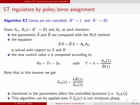
Algorithm E2 (zeros are not cancelled: B+ = 1 and B− = B)

Given Am, Bm(= B− = B) and A0, at each iteration:

the parameters A and B are computed with the RLS methodthe equation

A R + B S = A0 Am

is solved with respect to S and Rthe new control value u is computed according to

Ru = Tv − Sy , with T = k =Am(1)

B(1)

Note that in this manner we get

Gm(z) =kB(z)

Am(z)

Variations in the parameters affect the controlled dynamics (i.e. Gm(z))This algorithm can be applied even if Gp(z) is non minimum phase.




The above is the “explicit” formulation of the control design procedure. Anotherversion is the “implicit” one, where the parameters of the controller (not of theprocess) are estimated in real time. From

AR ′y + B−Sy = A0 Amy

Ay = Bu

we getA0 Amy = B R ′u + B−Sy = B−(Ru + Sy)

If B− = 1, then this equation is linear in the parameters of the R , S polynomials,and therefore the RLS algorithm can be used.

The overall procedure is simpler but can be applied only for minimum phasesystems, since all the zeros must be cancelled (B− = 1).




Algorithm I1 (zeros are cancelled)

Given Am, Bm and A0, at each iteration:

the parameters R and S of the model

A0Amy = Ru + Sy

are estimated with the RLS method

the new control input u is computed by

Ru = Tv − Sy

with T = k A0, k = Am(1) (as in E1).



ST regulators by poles/zeros assignment: Example

Let us consider a system described by

G(s) =0.4

(s + 1)(s + 2)(s + 0.2)=

Y (s)

U(s)

Open loop response to a unit step

0 5 10 15 20 25 30 35 40 45 500

0.2

0.4

0.6

0.8

1

t (s)

y(t)

Process output

Two design procedures will be exam-ined:

algorithm E2 (zeros not cancelled)

algorithm I1 (zeros cancelled)



ST regulators by poles/zeros assignment: Example

Let us assume that the following discrete-time model of the process is given

G(z) = z−1 b0 + b1z−1

1 + a1z−1=

Y (z)

U(z)→ y(k) = −a1y(k−1)+b0u(k−1)+b1u(k−2)

with a sampling period T = 1 s.

Moreover, define the desired polynomial Am(z) as

Am(z) = 1−2e−δωnT cosωnT√1−δ2z−1+e−2δωnT z−2

= 1 + c1z−1 + c2z

−2

in which the values δ = 0.7, ωn = 0.25 rad/s are considered.



ST regulators by poles/zeros assignment: Example – E2

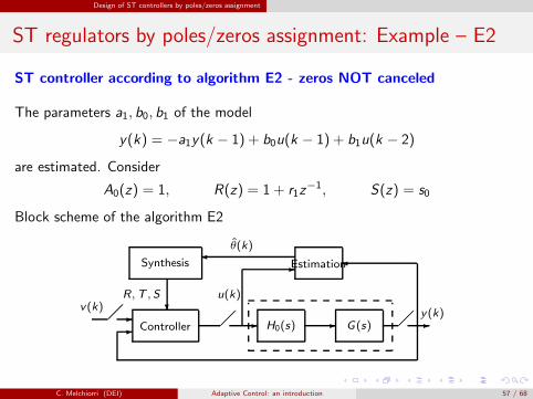
ST controller according to algorithm E2 - zeros NOT canceled

The parameters a1, b0, b1 of the model

y(k) = −a1y(k − 1) + b0u(k − 1) + b1u(k − 2)

are estimated. Consider

A0(z) = 1, R(z) = 1 + r1z−1, S(z) = s0

Block scheme of the algorithm E2

Controller H0(s) G(s)

EstimationSynthesis✛

❄

✲ ✛

✲✲ ��✲✲�� ✲

R,T ,S

θ(k)

y(k)v(k)

u(k)




The design equation is

(1 + a1z−1)(1 + r1z

−1) + z−1(b0 + b1z−1)s0 = 1 + c1z

−1 + c2z−2

→ 1 + (r1 + a1 + b0s0)z−1 + (a1r1 + b1s0)z

−2 = 1 + c1z−1 + c2z

−2

to be solved with respect to r1 and s0:

s0 = (c2 − a1c1 + a21)/(b1 − a1b0)

r1 = c1 − a1 − s0b0

The control equation is

(1 + r1z−1)u(k) = K v(k)− s0y(k)

from whichu(k) = K v(k)− s0y(k)− r1u(k − 1)

with K = (1 + c1 + c2)/(b0 + b1) (unit gain for Gm(z)).




System response with controller E2

0 20 40 60 80 100 120 140 160 180 200−2

−1

0

1

2

3Process output

0 20 40 60 80 100 120 140 160 180 200−2

−1

0

1

2

3

4

5

Time (s)

Control input u




System response with controller E2

0 20 40 60 80 100 120 140 160 180 2000.94

0.96

0.98

1Forgetting factor β

0 20 40 60 80 100 120 140 160 180 200−1

−0.5

0

0.5

1Plant parameters

a0b0b1

0 20 40 60 80 100 120 140 160 180 200−0.2

0

0.2

0.4

0.6

Time (s)

Prediction error

Forgetting factor β, estimation of the parameters a1, b0, b1 and estimation error. Note that theRLS algorithm gives satisfying results even at the second step of the reference signal.




System response with controller E2: variation of the process’s gain at t = 80 s.

0 20 40 60 80 100 120 140 160 180 200−2

−1

0

1

2

3Process output

0 20 40 60 80 100 120 140 160 180 200−2

−1

0

1

2

3

4

5

Time (s)

Control input u




System response with controller E2: variation of the process’s gain at t = 80 s.

0 20 40 60 80 100 120 140 160 180 2000.94

0.96

0.98

1Forgetting factor β

0 20 40 60 80 100 120 140 160 180 200−1

−0.5

0

0.5

1Plant parameters

a0b0b1

0 20 40 60 80 100 120 140 160 180 200−0.2

0

0.2

0.4

0.6

Time (s)

Prediction error




The discrete time model has been assumed as:

G(z) = z−1 b0 + b1z−1

1 + a1z−1=

Y (z)

U(z)→ y(k) = −a1y(k−1)+b0u(k−1)+b1u(k−2)

The final values of the parameters estimated by the RLS algorithm are:

In case of constant gain:

a1 = −0.850393, b0 = −0.135577, b1 = 0.286491

In case of variable gain:

a1 = −0.850609, b0 = −0.269460, b1 = 0.570891

In both cases:- the pole is p ≈ 0.85, stable- the zero is z = 2.11, → unstable!



ST regulators by poles/zeros assignment: Example – I1

ST controller according to algorithm I1 - zeros are canceled

Controller H0(s) G(s)

Estimation

❄

✲ ✛

✲✲ ✲✲ ✲y(k)v(k)

u(k)

R , S

By assuming

A0(z) = 1, R(z) = r0 + r1z−1, S(z) = s0 + s1z

−1

we get

(1+c1z−1+c2z

−2)y(k) = z−1[(r0+r1z−1)u(k)+(s0+s1z

−1)y(k)]




From which

y(k)+c1y(k − 1)+c2y(k − 2) =

= s0y(k − 1)+s1y(k − 2)+r0u(k − 1)+r1u(k − 2)

The parameters s0, s1, r0, r1 are estimated. One gets:

(r0 + r1z−1)u(k) = kv(k)− (s0 + s1z

−1)y(k)

and then

u(k) =1

r0[k v(k)− s0y(k)− s1y(k − 1)− r1u(k − 1)]

with k = 1 + c1 + c2.




System response with controller I1 and T = 1 s.

0 20 40 60 80 100 120 140 160 180 200-2

0

2

yr(t

), y

(t)

0 20 40 60 80 100 120 140 160 180 200-5

0

5

t (s)

un(t

)

Process output

Control variable

Unstable behaviour due to cancelation of non-minimum phase zero (z = −2.11).




System output with algorithm I1, T = 3 s.

0 20 40 60 80 100 120 140 160 180 200-2

0

2

yr(t

), y

(t)

0 20 40 60 80 100 120 140 160 180 200-2

0

2

t (s)

un(t

)

Process output

Control variable

With a higher sampling period, non-minimum phase zeros are absent.




0 20 40 60 80 100 120 140 160 180 2000.94

0.96

0.98

1be

ta(t)

0 20 40 60 80 100 120 140 160 180 200-1

0

1

alfa

(t)

Stima dei parametri

0 20 40 60 80 100 120 140 160 180 200

0

t (s)

es(t)

Prediction error

Forgetting factor


adaptive control: an introduction - unibo.it · pdf filein an adaptive control system, two...

Documents