adapted from c. bishop pattern recognition and machine...
TRANSCRIPT
Adapted from C. Bishop
PATTERN RECOGNITION AND MACHINE LEARNING CHAPTER 3: LINEAR MODELS FOR REGRESSION

Linear Basis Function Models (1)
Example: Polynomial Curve Fitting

Linear Basis Function Models (2)
Generally
where Áj(x) are known as basis functions.
Typically, Á0(x) = 1, so that w0 acts as a bias.
In the simplest case, we use linear basis functions : Ád(x) = xd.
Linear Basis Function Models (3)
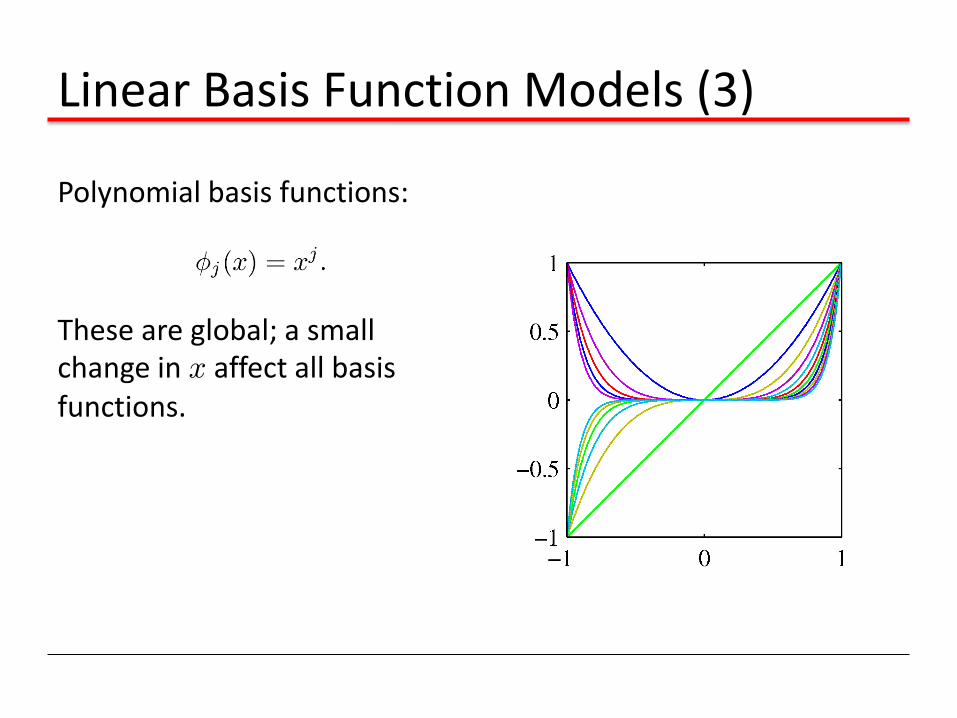
Polynomial basis functions:
These are global; a small change in x affect all basis functions.

Linear Basis Function Models (4)
Gaussian basis functions:
These are local; a small change in x only affects nearby basis functions. ¹j and s control location and scale (width).
Linear Basis Function Models (5)
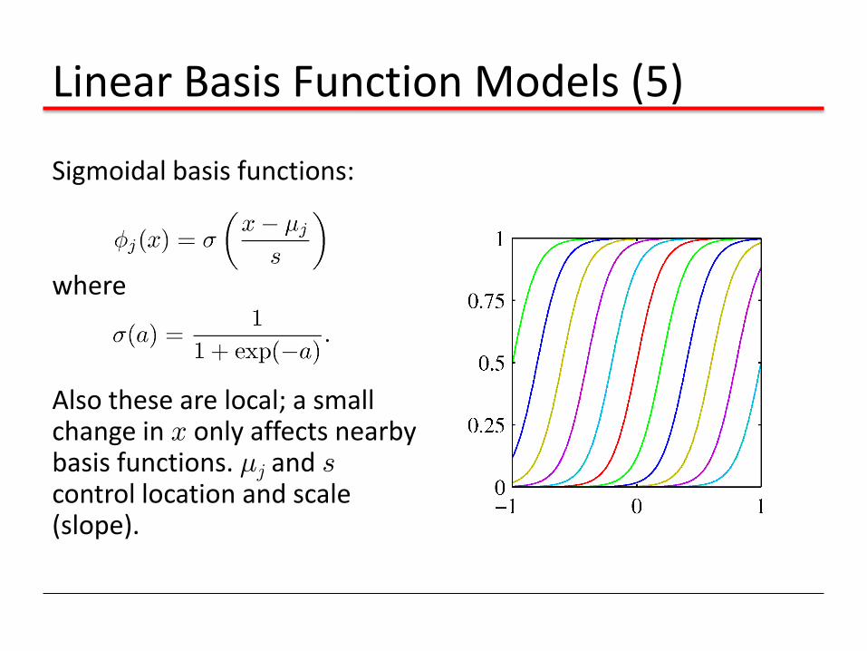
Sigmoidal basis functions:
where
Also these are local; a small change in x only affects nearby basis functions. ¹j and s control location and scale (slope).
Maximum Likelihood and Least Squares (1)
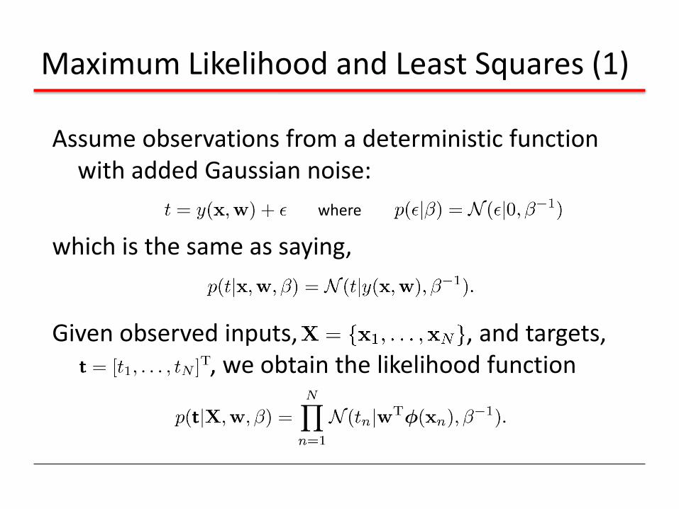
Assume observations from a deterministic function with added Gaussian noise:
which is the same as saying,
Given observed inputs, , and targets, , we obtain the likelihood function
where

Maximum Likelihood and Least Squares (2)
Taking the logarithm, we get
where
is the sum-of-squares error.

Computing the gradient and setting it to zero yields
Solving for w, we get
where
Maximum Likelihood and Least Squares (3)
The Moore-Penrose pseudo-inverse, .
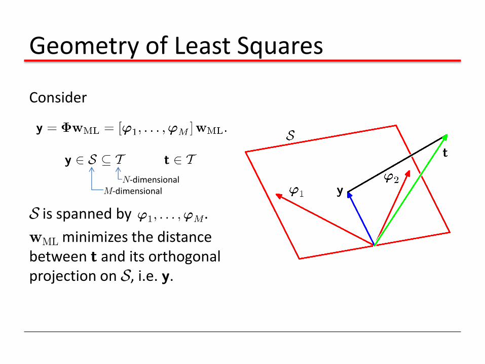
Geometry of Least Squares
Consider
S is spanned by .
wML minimizes the distance between t and its orthogonal projection on S, i.e. y.
N-dimensional M-dimensional

Sequential Learning
Data items considered one at a time (a.k.a. online learning); use stochastic (sequential) gradient descent:
This is known as the least-mean-squares (LMS) algorithm. Issue: how to choose ´?

Regularized Least Squares (1)
Consider the error function:
With the sum-of-squares error function and a quadratic regularizer, we get
which is minimized by
Data term + Regularization term
¸ is called the regularization coefficient.

Regularized Least Squares (2)
With a more general regularizer, we have
Lasso Quadratic

Regularized Least Squares (3)
Lasso tends to generate sparser solutions than a quadratic regularizer.

Regularized Least Squares (4)
λ increases => an increasing number of parameters are driven to zero
Advantages of RLS:
- Allows complex models to be trained on limited data without over-fitting
- Limits the effective model complexity
- No need to find the appropriate number of basis functions (can use complex models)
Disadvantages of RLS:
- We need to find the best value for the regularization coefficient λ
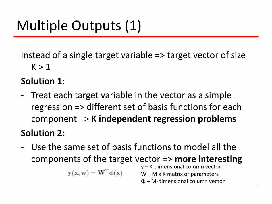
Multiple Outputs (1)
Instead of a single target variable => target vector of size K > 1
Solution 1:
- Treat each target variable in the vector as a simple regression => different set of basis functions for each component => K independent regression problems
Solution 2:
- Use the same set of basis functions to model all the components of the target vector => more interesting
y – K-dimensional column vector W – M x K matrix of parameters Φ – M-dimensional column vector
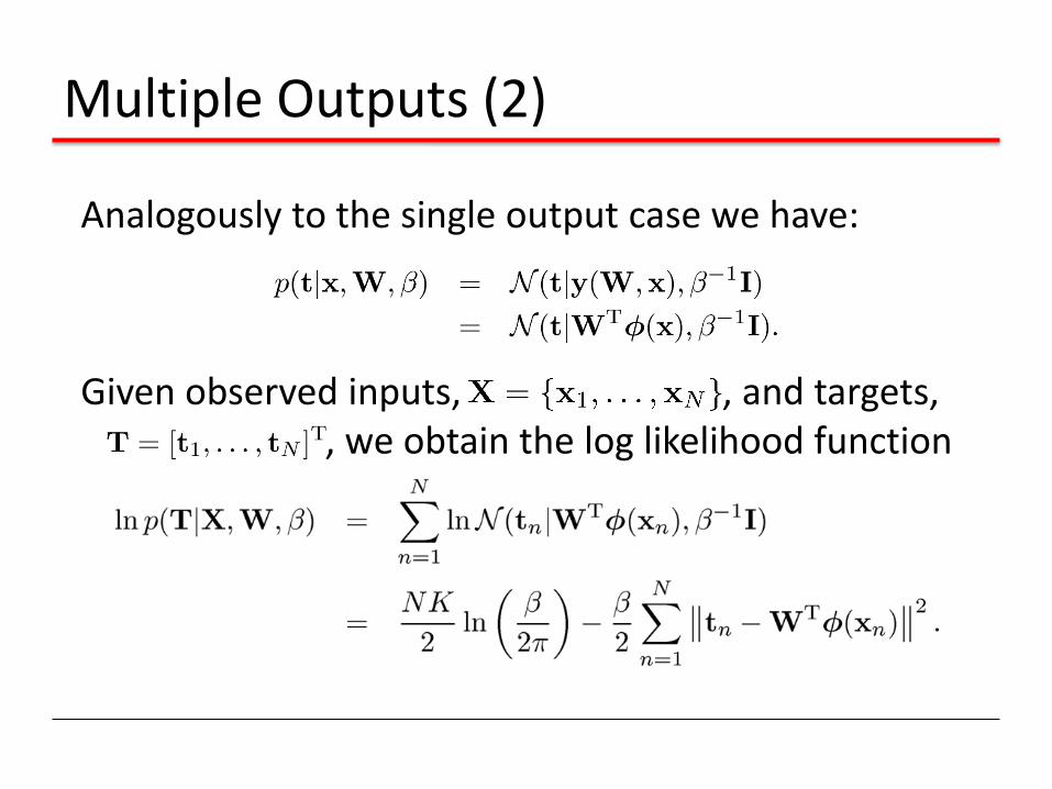
Multiple Outputs (2)
Analogously to the single output case we have:
Given observed inputs, , and targets, , we obtain the log likelihood function
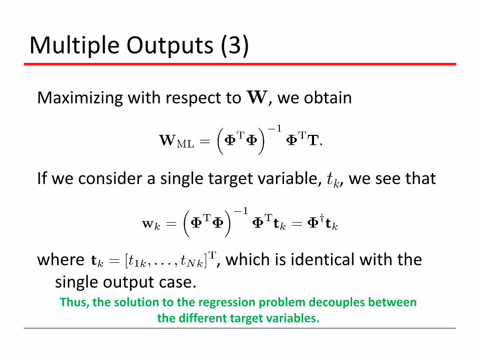
Multiple Outputs (3)
Maximizing with respect to W, we obtain
If we consider a single target variable, tk, we see that
where , which is identical with the single output case. Thus, the solution to the regression problem decouples between
the different target variables.
The Bias-Variance Decomposition (0)
How can we choose the best model for our data?
- How to choose M ?
- M too large => over-fitting
- M too small => cannot capture interesting trends in the data
- Use regularization – how to choose λ ?
Solution: over-fitting is an effect of using maximum likelihood, it does not appear when using a Bayesian model…
Before that, let’s use a frequentist viewpoint of the model complexity issue, called bias-variance trade-off

The Bias-Variance Decomposition (1)
Recall the expected squared loss,
Where the optimal prediction:
The second term of E[L] corresponds to the noise
inherent in the random variable t.
What about the first term?

The Bias-Variance Decomposition (1’)
We want to minimize the first term
- If we would have had an infinity of training points and a lot of computational resources, the best thing to do is to determine h(x) with a very good accuracy => optimal choice for y(x)
- As we only have a finite set of training points, the regression function h(x) cannot be computed exactly
The second one is inherent to the noise in the training data and cannot be eliminated (as it does not depend of our choice of y(x))

The Bias-Variance Decomposition (2)
Suppose we were given multiple data sets, each of size N. Any particular data set, D, will give a particular function y(x;D). We then have

The Bias-Variance Decomposition (3)
Taking the expectation over D yields The first term, called the squared bias, represents the
extent to which the average prediction over all data sets differs from the desired regression function.
The second term, called the variance, measures the extent to which the solutions for individual data sets vary around their average, and hence this measures the extent to which the function y(x;D) is sensitive to the particular choice of data set.
The Bias-Variance Decomposition (4)
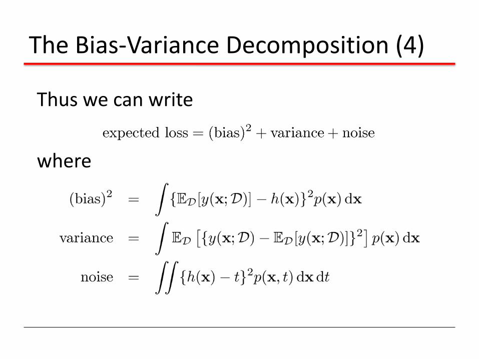
Thus we can write
where
The Bias-Variance Decomposition (4’)
Objective: minimize the expected loss, which we have decomposed into the sum of a (squared) bias, a variance, and a constant noise term
- trade-off between bias and variance - very flexible models having low bias and high variance - rigid models having high bias and low variance
The model with the optimal predictive capability is the one that leads to the best balance between bias
and variance.

The Bias-Variance Decomposition (5)
Example: 25 data sets from the sinusoidal, varying the degree of regularization, ¸.
- each has 25 data points and 24 Gaussian basis functions
- right picture shows the average over 100 data sets
λ large => high bias, low variance

The Bias-Variance Decomposition (6)
Example: 25 data sets from the sinusoidal, varying the degree of regularization, ¸.

The Bias-Variance Decomposition (7)
Example: 25 data sets from the sinusoidal, varying the degree of regularization, ¸.
λ small=> low bias, high variance
The Bias-Variance Trade-off
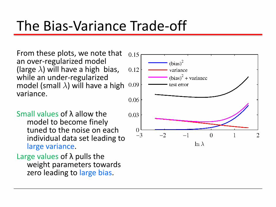
From these plots, we note that an over-regularized model (large ¸) will have a high bias, while an under-regularized model (small ¸) will have a high variance. Small values of λ allow the
model to become finely tuned to the noise on each individual data set leading to large variance.
Large values of λ pulls the weight parameters towards zero leading to large bias.

The Bias-Variance Trade-off (2)

The Bias-Variance Trade-off (3)
The result of averaging many solutions for the complex model with M = 25 is a very good fit to the regression function
=> averaging may be a beneficial procedure
=> difficult in practice, as needed a large training set to be split in multiple training sets
Indeed, a weighted averaging of multiple solutions lies at the heart of a Bayesian approach
=> the averaging is with respect to the posterior distribution of parameters, not with respect to multiple data sets.
Bayesian Linear Regression (0)
1. Used to escape from the over-fitting problem of ML
2. Leads to automatic models of determining the model complexity given the training data alone
The posterior distribution p(w|t) is proportional to the product of the likelihood function p(t|w) and
the prior p(w)
Bayesian Linear Regression (1)
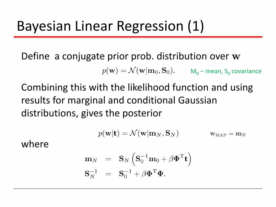
Define a conjugate prior prob. distribution over w
Combining this with the likelihood function and using results for marginal and conditional Gaussian distributions, gives the posterior
where
M0 – mean, S0 covariance

Bayesian Linear Regression (2)
A common choice for the prior is for which The log of the posterior distribution is given by the sum of the log likelihood and the log of the prior: Next we consider an example …

Bayesian Linear Regression (3)
Example: straight line fitting, linear basis function model
0 data points observed
Prior Data Space

Bayesian Linear Regression (4)
1 data point observed
Likelihood Posterior Data Space

Bayesian Linear Regression (5)
2 data points observed
Likelihood Posterior Data Space

Bayesian Linear Regression (6)
20 data points observed
Likelihood Posterior Data Space

Predictive Distribution (1)
Predict t for new values of x by integrating over w:
where
Noise in data + uncertainty associated with the parameters w

Remarks
Noise + distribution of w – independent Gaussians => their variances are additive
As additional data points are observed, the posterior distribution becomes narrower
Thus, if N -> INFINITY:
- second term goes to zero
- the variance of the predictive distribution arises only from the noise
Predictive Distribution (2)
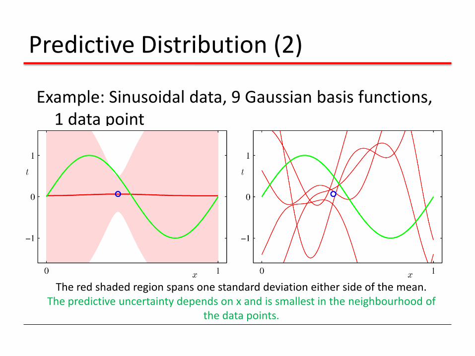
Example: Sinusoidal data, 9 Gaussian basis functions, 1 data point
The red shaded region spans one standard deviation either side of the mean. The predictive uncertainty depends on x and is smallest in the neighbourhood of
the data points.
Predictive Distribution (3)
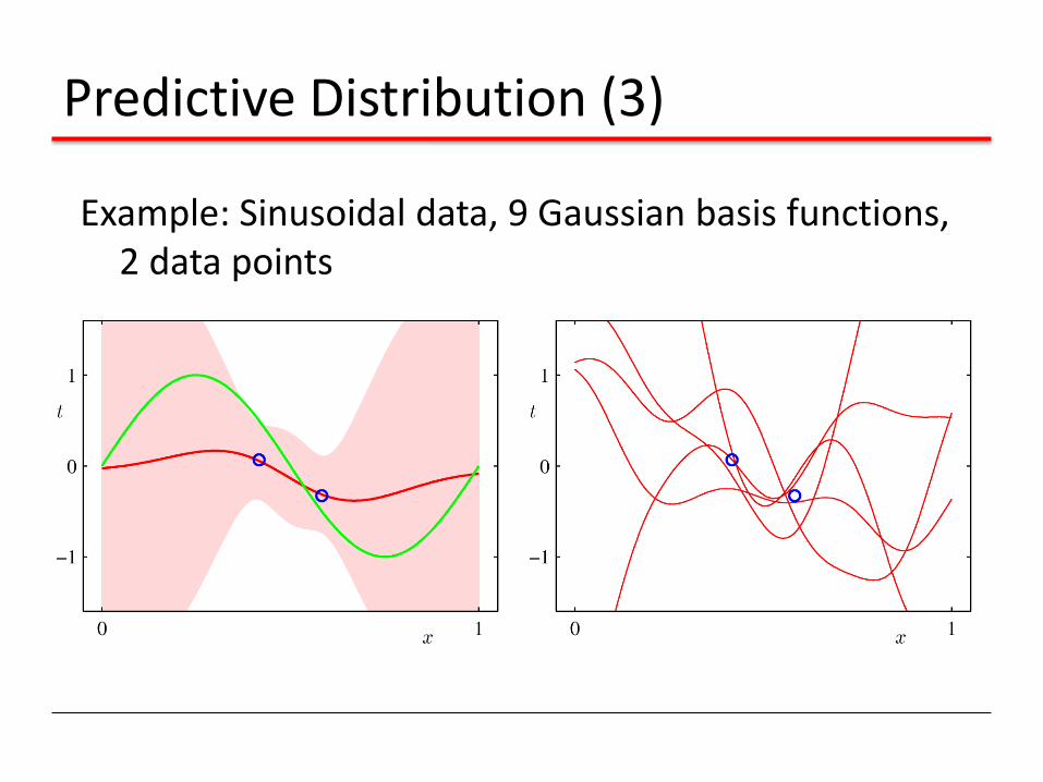
Example: Sinusoidal data, 9 Gaussian basis functions, 2 data points

Predictive Distribution (4)
Example: Sinusoidal data, 9 Gaussian basis functions, 4 data points
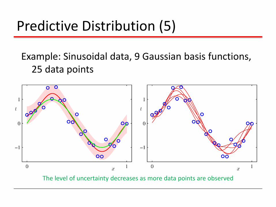
Predictive Distribution (5)
Example: Sinusoidal data, 9 Gaussian basis functions, 25 data points
The level of uncertainty decreases as more data points are observed
Equivalent Kernel (1)
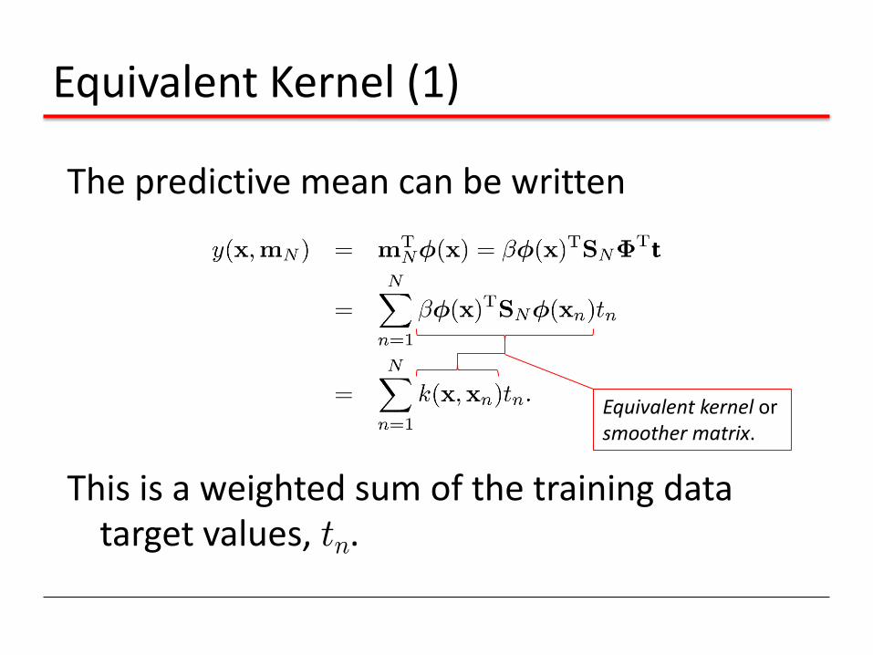
The predictive mean can be written
This is a weighted sum of the training data target values, tn.
Equivalent kernel or smoother matrix.

Equivalent Kernel (2)
Weight of tn depends on distance between x and xn; nearby xn carry more weight.

Equivalent Kernel (3)
Non-local basis functions have local equivalent kernels:
Polynomial Sigmoidal
Equivalent Kernel (4)
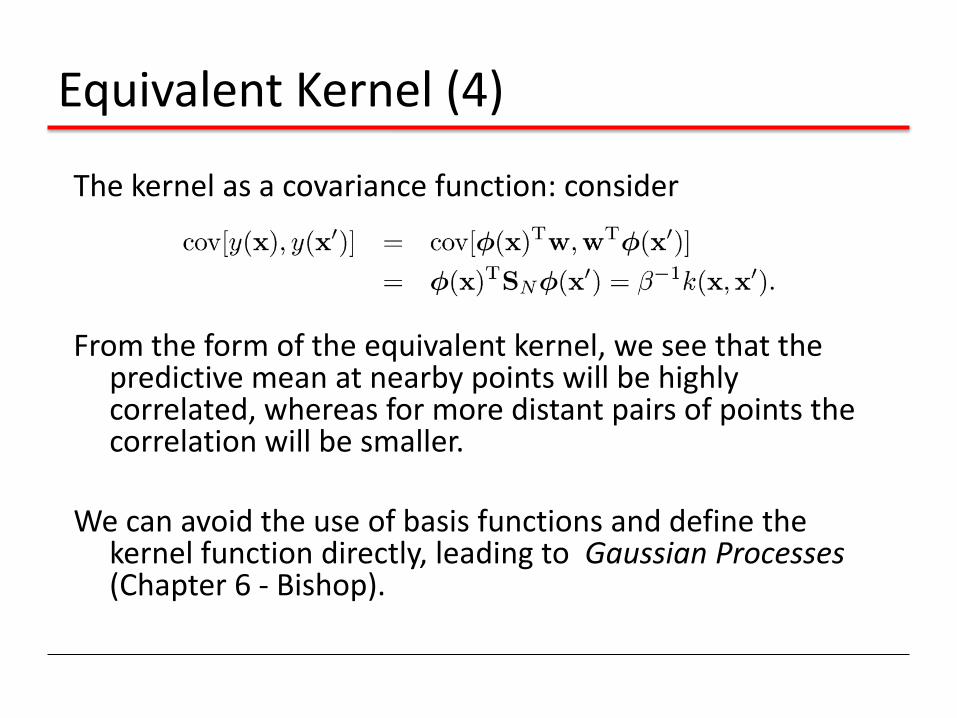
The kernel as a covariance function: consider From the form of the equivalent kernel, we see that the
predictive mean at nearby points will be highly correlated, whereas for more distant pairs of points the correlation will be smaller.
We can avoid the use of basis functions and define the
kernel function directly, leading to Gaussian Processes (Chapter 6 - Bishop).
Equivalent Kernel (5)
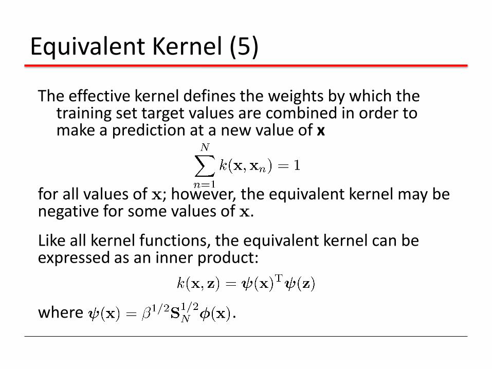
The effective kernel defines the weights by which the training set target values are combined in order to make a prediction at a new value of x
for all values of x; however, the equivalent kernel may be negative for some values of x.
Like all kernel functions, the equivalent kernel can be expressed as an inner product:
where .

Bayesian Model Comparison (1)
How do we choose the ‘right’ model?
Assume we want to compare models Mi, i=1, …,L, using data D; this requires computing
Bayes Factor: ratio of evidence for two models
Posterior Prior Model evidence or marginal likelihood
Bayesian Model Comparison (2)
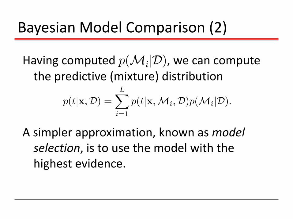
Having computed p(MijD), we can compute the predictive (mixture) distribution
A simpler approximation, known as model selection, is to use the model with the highest evidence.
Bayesian Model Comparison (3)
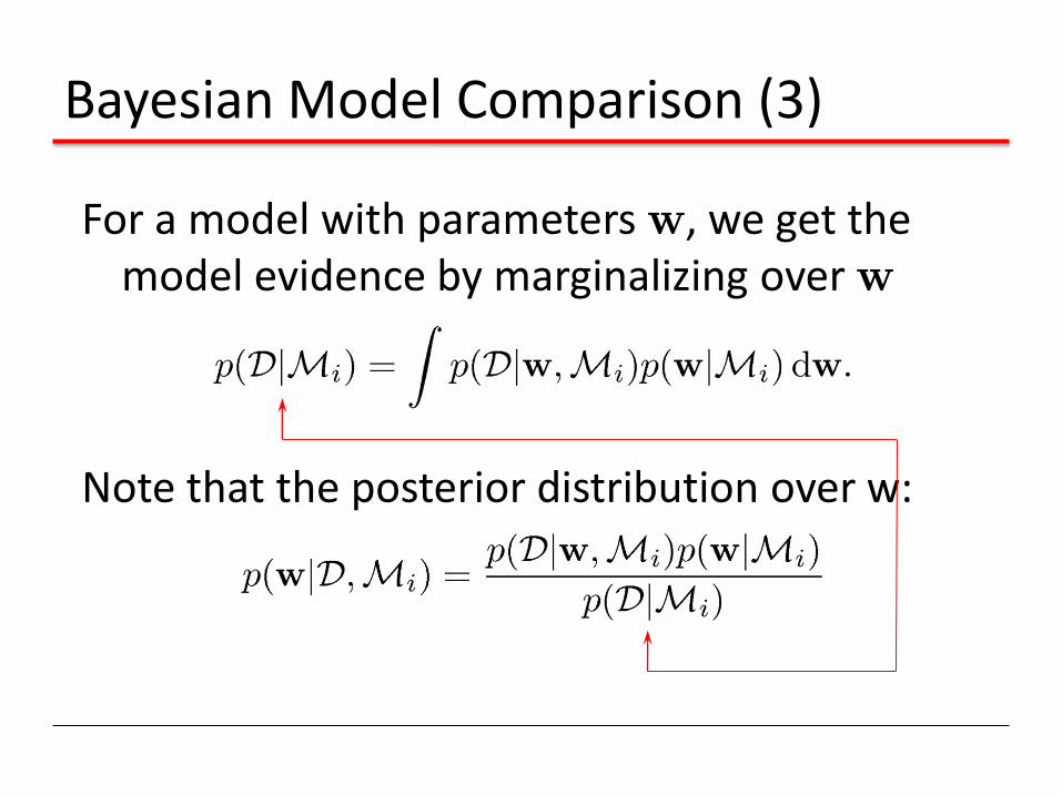
For a model with parameters w, we get the model evidence by marginalizing over w
Note that the posterior distribution over w:
Bayesian Model Comparison (4)
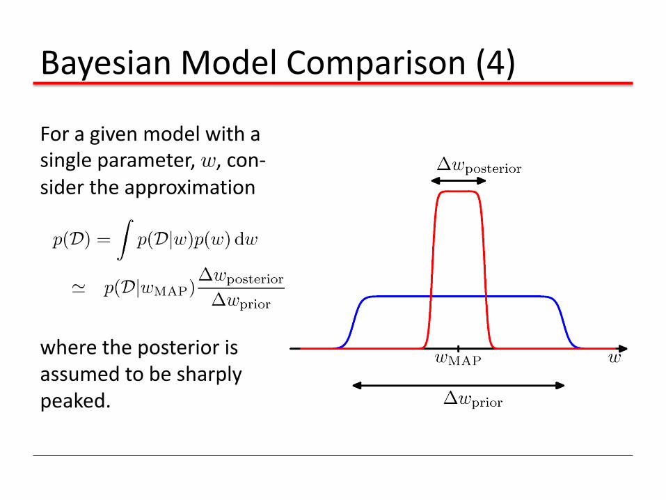
For a given model with a single parameter, w, con-sider the approximation
where the posterior is assumed to be sharply peaked.

Bayesian Model Comparison (5)
Taking logarithms, we obtain
With M parameters, all assumed to have the same ratio , we get
Negative
Negative and linear in M.

Bayesian Model Comparison (6)
The first term represents the fit to the data given by the most probable parameter values, and for a flat prior this would correspond to the log likelihood.
The second term penalizes the model according to
its complexity.
< 1
If parameters are finely tuned to the data in the posterior distribution, then the penalty term is large.

Bayesian Model Comparison (7)
Matching data and model complexity

Bayesian Model Comparison (8)
This approach permits us to choose the best model, given the training data
However, in a practical application, it will be wise to keep aside an independent test set of data on which to evaluate the overall performance of the final system

Optional Slides
Not required for the SSL exam!

The Evidence Approximation (1)
The fully Bayesian predictive distribution is given by
but this integral is intractable. Approximate with
where is the mode of , which is assumed to
be sharply peaked; a.k.a. empirical Bayes, type II or gene-
ralized maximum likelihood, or evidence approximation.

The Evidence Approximation (2)
From Bayes’ theorem we have
and if we assume p(®,¯) to be flat we see that
General results for Gaussian integrals give

The Evidence Approximation (3)
Example: sinusoidal data, M th degree polynomial,

Maximizing the Evidence Function (1)
To maximise w.r.t. ® and ¯, we define the eigenvector equation
Thus
has eigenvalues ¸i + ®.

Maximizing the Evidence Function (2)
We can now differentiate w.r.t. ® and ¯, and set the results to zero, to get
where
N.B. ° depends on both ® and ¯.

Effective Number of Parameters (3)
Likelihood
Prior
w1 is not well determined by the likelihood
w2 is well determined by the likelihood ° is the number of well determined parameters

Effective Number of Parameters (2)
Example: sinusoidal data, 9 Gaussian basis functions, ¯ = 11.1.

Effective Number of Parameters (3)
Example: sinusoidal data, 9 Gaussian basis functions, ¯ = 11.1.
Test set error

Effective Number of Parameters (4)
Example: sinusoidal data, 9 Gaussian basis functions, ¯ = 11.1.
Effective Number of Parameters (5)
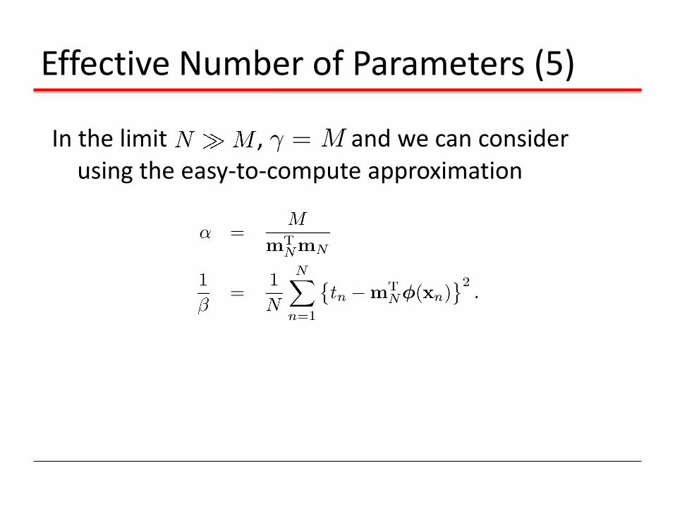
In the limit , ° = M and we can consider using the easy-to-compute approximation

Limitations of Fixed Basis Functions
• M basis function along each dimension of a D-dimensional input space requires MD basis functions: the curse of dimensionality.
• In later chapters, we shall see how we can get away with fewer basis functions, by choosing these using the training data.