ADAPS: Autonomous Driving Via Principled Simulations

Weizi Li1, David Wolinski1, and Ming C. Lin1,2

Abstract— Autonomous driving has gained significant ad-vancements in recent years. However, obtaining a robust controlpolicy for driving remains challenging as it requires trainingdata from a variety of scenarios, including rare situations (e.g.,accidents), an effective policy architecture, and an efficientlearning mechanism. We propose ADAPS for producing robustcontrol policies for autonomous vehicles. ADAPS consists of twosimulation platforms in generating and analyzing accidents toautomatically produce labeled training data, and a memory-enabled hierarchical control policy. Additionally, ADAPS offersa more efficient online learning mechanism that reduces thenumber of iterations required in learning compared to existingmethods such as DAGGER [1]. We present both theoreticaland experimental results. The latter are produced in simulatedenvironments, where qualitative and quantitative results aregenerated to demonstrate the benefits of ADAPS.

I. INTRODUCTION

Autonomous driving consists of many complex sub-tasksthat consider the dynamics of an environment and oftenlack accurate definitions of various driving behaviors. Thesecharacteristics lead to conventional control methods to suffersubpar performance on the task [2], [3]. However, drivingand many other tasks can be easily demonstrated by humanexperts. This observation inspires imitation learning, whichleverages expert demonstrations to synthesize a controller.

While there are many advantages of using imitation learn-ing, it also has drawbacks. For autonomous driving, themost critical one is covariate shift, meaning the training andtest distributions are different. This could lead autonomousvehicles (AVs) to accidents since a learned policy may failto respond to unseen scenarios including those dangeroussituations that do not occur often.

In order to mitigate this issue, the training dataset needsto be augmented with more expert demonstrations coveringa wide spectrum of driving scenarios—especially ones ofsignificant safety threats to the passengers—so that a policycan learn how to recover from its own mistakes. This isemphasized by Pomerleau [4], who synthesized a neuralnetwork based controller for AVs: “the network must notsolely be shown examples of accurate driving, but also howto recover (i.e. return to the road center) once a mistake hasbeen made.”

Although critical, obtaining recovery data from accidentsin the physical world is impractical due to the high cost of avehicle and potential injuries to both passengers and pedestri-ans. In addition, even one managed to collect accident data,

1W. Li, D. Wolinski, M. Lin are with the Department of Com-puter Science, University of North Carolina at Chapel Hill, NC, USA{weizili,dwolinsk,lin}@cs.unc.edu

2M. Lin is now with the Department of Computer Science, University ofMaryland at College Park, MD, USA lin@cs.umd.edu

human experts are usually needed to label them, which isinefficient and may subject to judgmental errors [5].

These difficulties naturally lead us to the virtual world,where accidents can be simulated and analyzed [6]. We havedeveloped ADAPS (Autonomous Driving Via PrincipledSimulations) to achieve this goal. ADAPS consists of twosimulation platforms and a memory-enabled hierarchicalcontrol policy based on deep neural networks (DNNs). Thefirst simulation platform, referred to as SimLearner, runs in a3D environment and is used to test a learned policy, simulateaccidents, and collect training data. The second simulationplatform, referred to as SimExpert, acts in a 2D environmentand serves as the “expert” to analyze and resolve an accidentvia principled simulations that can plan alternative safetrajectories for a vehicle by taking its physical, kinematic,and geometric constraints into account.

Furthermore, ADAPS represents a more efficient onlinelearning mechanism than existing methods such as DAG-GER [1]. This is useful consider learning to drive requiresiterative testing and update of a control policy. Ideally, wewant to obtain a robust policy using minimal iterationssince one iteration corresponds to one incident. This wouldrequire the generation of training data at each iteration to beaccurate, efficient, and sufficient so that a policy can gain alarge improvement going into the next iteration. ADAPS canassist to achieve this goal.

The main contributions of this research are specifically:(1) The accidents generated in SimLearner will be analyzedby SimExpert to produce alternative safe trajectories. (2)These trajectories will be automatically processed to gen-erate a large number of annotated and segmented trainingdata. Because SimExpert is parameterized and has taken thephysical, kinematic, and geometric constraints of a vehicleinto account (i.e., principled), the resulting training examplesare more heterogeneous than data collected via running alearned policy multiple times and are more effective thandata collected through random sampling. (3) We presentboth theoretical and experimental results to demonstrate thatADAPS is an efficient online learning mechanism.

The Appendix, which contains supporting material, can befound at http://gamma.cs.unc.edu/ADAPS/.

II. RELATED WORK

We sample previous studies that are related to each aspectof our framework and discuss the differences within.

Autonomous Driving. Among various methods to planand control an AV [7], we focus on end-to-end imitationlearning as it can avoid manually designed features andlead to a more compact policy compared to conventional

mediation perception approaches [8]. The early studies doneby Pomerleau [4] and LeCun et al. [9] have shown that neuralnetworks can be used for an AV to achieve lane-followingand off-road obstacle avoidance. Due to the advancementsof deep neural networks (DNNs), a number of studies haveemerged [10], [11], [12], [13]. While significant improve-ments have been made, these results mainly inherit normaldriving conditions and restrict a vehicle to the lane-followingbehavior [13]. Our policy, in contrast, learns from accidentsand enables a vehicle to achieve on-road collision avoidancewith both static and dynamic obstacles.

Hierarchical Control Policy. There have been manyefforts in constructing a hierarchical policy to control anagent at different stages of a task [14]. Example studiesinclude the options framework [15] and transferable motorskills [16]. When combined with DNNs, the hierarchicalapproach has been adopted for virtual characters to learnlocomotion tasks [17]. In these studies, the goal is to discovera hierarchical relationship from complex sensorimotor behav-iors. We apply a hierarchical and memory-enabled policy toautonomous driving based on multiple DNNs. Our policyenables an AV to continuously categorize the road conditionas safe or dangerous, and execute corresponding controlcommands to achieve accident-free driving.

Generative Policy Learning. Using principled simula-tions to assist learning is essentially taking a generativemodel approach. Several studies have adopted the samephilosophy to learn (near-)optimal policy, examples includingfunction approximations [18], Sparse Sampling [19], andFitted Value Iteration [20]. These studies leverage a gener-ative model to stochastically generate training samples. Theemphasize is to simulate the feedback from an environmentinstead of the dynamics of an agent assuming the rewardfunction is known. Our system, on the other hand, doesnot assume any reward function of a driving behavior butmodels the physical, kinematic, and geometric constraints ofa vehicle, and uses simulations to plan their trajectories w.r.t.environment characteristics. In essence, our method learnsfrom expert demonstrations rather than self-exploration [21]as of the previous studies.

III. PRELIMINARIES

Autonomous driving is a sequential prediction and con-trolled (SPC) task, for which a system must predict asequence of control commands based on inputs that dependon past predicted control commands. Because the controland prediction processes are intertwined, SPC tasks oftenencounter covariate shift, meaning the training and testdistributions vary. In this section, we will first introducenotation and definitions to formulate an SPC task and thenbriefly discuss its existing solutions.

A. Notation and Definitions

The problem we consider is a T -step control task. Giventhe observation φ = φ(s) of a state s at each step t ∈ [[1, T ]],the goal of a learner is to find a policy π ∈ Π such that itsproduced action a = π(φ) will lead to the minimal cost:

π = arg minπ∈Π

T∑t=1

C (st, at) , (1)

where C (s, a) is the expected immediate cost of performinga in s. For many tasks such as driving, we may not knowthe true value of C. So, we instead minimize the observedsurrogate loss l(φ, π, a∗), which is assumed to upper boundC, based on the approximation of the learner’s action a =π(φ) to the expert’s action a∗ = π∗(φ). We denote thedistribution of observations at t as dtπ , which is the result ofexecuting π from 1 to t−1. Consequently, dπ = 1

T

∑Tt=1 d

tπ

is the average distribution of observations by executing π forT steps. Our goal is to solve an SPC task by obtaining π thatminimizes the observed surrogate loss under its own inducedobservations w.r.t. expert’s actions in those observations:

π = arg minπ∈Π

Eφ∼dπ,a∗∼π∗(φ) [l (φ, π, a∗)] . (2)

We further denote ε = Eφ∼dπ∗ ,a∗∼π∗(φ) [l (φ, π, a∗)] as theexpected loss under the training distribution induced by theexpert’s policy π∗, and the cost-to-go over T steps of πas J (π) and of π∗ as J (π∗). It has been shown that bysimply treating expert demonstrations as i.i.d. samples thediscrepancy between J (π) and J (π∗) is O(T 2ε) [22], [1].Given the error of a typical supervised learning is O (Tε),this demonstrates the additional cost due to covariate shiftwhen solving an SPC task via standard supervised learning1.

B. Existing Techniques

Several approaches have been proposed to solve SPC tasksusing supervised learning while keeping the error growinglinearly instead of quadratically with T [22], [1], [23].Essentially, these methods reduce an SPC task to onlinelearning. By further leveraging interactions with experts andno-regret algorithms that have strong guarantees on convexloss functions [24], at each iteration, these methods train oneor multiple policies using standard supervised learning andimprove the trained policies as the iteration continues.

To illustrate, we denote the best policy at the ith iteration(trained using all observations from the previous i − 1iterations) as πi and for any policy π ∈ Π we have itsexpected loss under the observation distribution induced byπi as li (π) = Eφ∼dπi ,a∗∼π∗(φ) [li (φ, π, a∗)] , li ∈ [0, lmax]2.In addition, we denote the minimal loss in hindsight afterN ≥ i iterations as εmin = minπ∈Π

1N

∑Ni=1 li(π) (i.e., the

training loss after using all observations from N iterations).Then, we can represent the average regret of this onlinelearning program as εregret = 1

N

∑Ni=1 li(πi)− εmin. Using

DAGGER [1] as an example method, the accumulated errordifference becomes the summation of three terms:

J (π) ≤ Tεmin + Tεregret +O(f (T, lmax)

N), (3)

1The proofs regarding results O(T 2ε) and O(Tε) can be found inAppendix IX-A.

2In online learning, the surrogate loss l can be seen as chosen by someadversary which varies at each iteration.

where f (·) is the function of fixed T and lmax. As N →∞,the third term tends to 0 so as the second term if a no-regretalgorithm such as the Follow-the-Leader [25] is used.

The aforementioned approach provides a practical way tosolve SPC tasks. However, it may require many iterationsfor obtaining a good policy. In addition, usually humanexperts or pre-defined controllers are needed for labeling thegenerated training data, which could be inefficient or difficultto generalize. For autonomous driving, we want the iterationnumber to be minimal since it directly corresponds to thenumber of accidents. This requires the generation of trainingdata being accurate, efficient, and sufficient.

IV. ADAPS

In the following, we present theoretical analysis of ourframework and introduce our framework pipeline.

A. Theoretical Analysis

We have evaluated our approach against existing learningmechanisms such as DAGGER [1], with our method’s resultsproving to be more effective. Specifically, DAGGER [1]assumes that an underlying learning algorithm has access toa reset model. So, the training examples can be obtained onlyonline by putting an agent to its initial state distribution andexecuting a learned policy, thus achieving “small changes”at each iteration [1], [23], [26], [27]. In comparison, ourmethod allows a learning algorithm to access a generativemodel so that the training examples can be acquired offlineby putting an agent to arbitrary states during the analysisof an accident and letting a generative model simulate itsbehavior. This approach results in massive training data, thusachieving “large changes” of a policy at one iteration.

Additionally, existing techniques such as DAGGER [1]usually incorporate the demonstrations of a few experts intotraining. Because of the reset model assumption and the lackof a diversity requirement on experts, these demonstrationscan be homogeneous. In contrast, using our parameterizedmodel to retrace and analyze each accident, the number of re-covery actions obtained can be multiple orders of magnitudehigher. Subsequently, we can treat the generated trajectoriesand the additional data generated based on them (describedin Section VI-B) as running a learned policy to sampleindependent expert trajectories at different states, since 1)a policy that is learned using DNNs can achieve a smalltraining error and 2) our model provides near-exhaustivecoverage of the configuration space of a vehicle. With theseassumptions, we derive the following theorem.

Theorem 1: If the surrogate loss l upper bounds the truecost C, by collecting K trajectories using ADAPS at eachiteration, with probability at least 1−µ, µ ∈ (0, 1), we havethe following guarantee:

J (π) ≤ J (π) ≤ T εmin+T εregret+O

T lmax√

log 1µ

KN

.

Proof: See Appendix IX-A.3.Theorem 1 provides a bound for the expected cost-to-go of

the best learned policy π based on the empirical error of the

best policy in Π (i.e., εmin) and the empirical average regretof the learner (i.e., εregret). The second term can be elimi-nated if a no-regret algorithm such as Follow-the-Leader [25]is used and the third term suggests that we need the numberof training examples KN to be O

(T 2l2max log 1

µ

)in order

to have a negligible generalization error, which is easilyachievable using ADAPS. Summarizing these changes, wederive the following Corollary.

Corollary 1: If l is convex in π for any s and it up-per bounds C, and Follow-the-Leader is used to selectthe learned policy, then for any ε > 0, after collecting

O(T 2l2max log 1

µ

ε2

)training examples, with probability at least

1− µ, µ ∈ (0, 1), we have the following guarantee:

J (π) ≤ J (π) ≤ T εmin +O (ε) .

Proof: Following Theorem 1 and the aforementioneddeduction.

Now we only need the best policy to have a small trainingerror εmin. This can be achieved using DNNs since they haverich representing capabilities.

B. Framework PipelineThe pipeline of our framework is the following. First, in

SimLearner, we test a learned policy by letting it controlan AV. During the testing, an accident may occur, in whichcase the trajectory of the vehicle and the full specifications ofthe situation (e.g., positions of obstacles, road configuration,etc.) are known. Next, we switch to SimExpert and replicatethe specifications of the accident so that we can “solve” theaccident (i.e., find alternative safe trajectories and dangerouszones). After obtaining the solutions, we then use them togenerate additional training data in SimLearner, which willbe combined with previously generated data to update thepolicy. Finally, we test the updated policy again.

V. POLICY LEARNING

In this section, we will detail our control policy by firstexplaining our design rationale then formulating our problemand introducing the training data collection.

Driving is a hierarchical decision process. In its simplestform, a driver needs to constantly monitor the road condition,decide it is “safe” or “dangerous”, and make correspondingmaneuvers. When designing a control policy for AVs, weneed to consider this hierarchical aspect. In addition, drivingis a temporal behavior. Drivers need reaction time to respondto various road situations [28], [29]. A Markovian-basedcontrol policy will not model this aspect and instead likelyto give a vehicle jerky motions. Consider these factors, wepropose a hierarchical and memory-enabled control policy.

The task we consider is autonomous driving via a singlefront-facing camera. Our control policy consists of threemodules: Detection, Following, and Avoidance. The Detec-tion module keeps monitoring road conditions and activateseither Following or Avoidance to produce a steering com-mand. All these modules are trained via end-to-end imitationlearning and share a similar network specification which isdetailed in Appendix IX-B.

A. End-to-end Imitation Learning

The objective of imitation learning is to train a modelthat behaves or makes decisions like an expert throughdemonstrations. The model could be a classifier or a regresserπ parameterized by θπ:

θ = arg minθπ

T∑t=1

F (π (φt; θπ) , a∗t ) , (4)

where F is a distance function.The end-to-end aspect denotes the mapping from raw

observations to decision/control commands. For our policy,we need one decision module πDetection and two controlmodules πFollowing and πAvoidance. The input for πDetectionis a sequence of annotated images while the outputs arebinary labels indicating whether a road condition is danger-ous or safe. The inputs for πFollowing and πAvoidance aresequences of annotated images while the outputs are steeringangles. Together, these learned policies form a hierarchicalcontrol mechanism enabling an AV to drive safely on roadsand avoid obstacles when needed.

B. Training Data Collection

For training Following, inspired by the technique used byBojarski et al. [10], we collect images from three front-facingcameras behind the main windshield: one at the center, oneat the left side, and one at the right side. The image fromthe center camera is labeled with the exact steering anglewhile the images from the other two cameras are labeled withadjusted steering angles. However, once Following is learned,it only needs images from the center camera to operate.

For training Avoidance, we rely on SimExpert, which cangenerate numerous intermediate collision-free trajectoriesbetween the first moment and the last moment of a potentialaccident (see Section VI-A). By positioning an AV on thesetrajectories, we collect images from the center front-facingcamera along with corresponding steering angles. The train-ing of Detection requires a more sophisticated mechanismand is the subject of the next section.

VI. LEARNING FROM ACCIDENTS

We explain how we analyze an accident in SimExpert anduse the generated data to train the Avoidance and Detectionmodules of our policy. SimExpert is built based on the multi-agent simulator WarpDriver [30].

A. Solving Accidents

When an accident occurs, we know the trajectory of thetested vehicle for the latest K frames, which we note as acollection of states S =

⋃k∈[[1,K]] sk, where each state sk ∈

R4 contains the 2-dimensional position and velocity vectorsof the vehicle. Then, there are three notable states on thistrajectory that we need to track. The first is the earliest statewhere the vehicle involved in an accident (is in a collision)ska (at frame ka). The second is the last state skl (at framekl) where the expert algorithm can still avoid a collision. Thefinal one is the first state skf (at frame kf ) where the expert

Fig. 1. Illustration of important points and DANGER/SAFE labels fromSection VI for a vehicle traveling on the right lane of a straight road, withan obstacle in front. Labels are shown for four points {lu1, lu2, lu3, lu4}illustrating the four possible cases.

algorithm perceives the interaction leading to the accidentwith the other involved agent, before that accident.

In order to compute these notable states, we brieflyrecall the high-level components of WarpDriver [30]. Thiscollision-avoidance algorithm consists of two parts. The firstis the function p, which given the current state of an agentsk and any prediction point x ∈ R3 in 2-dimensional spaceand time (in this agent’s referential), gives the probability ofthat agent’s colliding with any neighbor p(sk,x) ∈ [0, 1].The second part is the solver, which based on this function,computes the agent’s probability of colliding with neighborsalong its future trajectory starting from a state sk (i.e., com-puted for x spanning the future predicted trajectory of theagent, we denote this probability P (sk)), and then proposesa new velocity to lower this probability. Subsequently, wecan initialize an agent in this algorithm to any state sk ∈ Sand compute a new trajectory consisting of K new statesSk =

⋃k∈[[1,K]] sk, where s1 = sk.

Additionally, since x = (0, 0, 0) in space and time inan agent’s referential represents the agent’s position at thecurrent time (we can use this point x with function p todetermine if the agent is currently colliding with anyone),we find ska where ka = min(k) subject to k ∈ [[1,K]]and p(sk, (0, 0, 0)) > 0. We note that a trajectory Skproduced by the expert algorithm could contain collisions(accounting for vehicle dynamics) depending on the statesk that it was initialized from. We can denote the set ofcolliding states along this trajectory as coll(Sk) = {sk ∈Sk | p(sk, (0, 0, 0)) > 0}. Then, we can compute skl wherekl = max(k) subject to k ∈ [[1, ka]] and coll(Sk) = ∅.Finally, we can compute skf with kf = 1 +max(k) subjectto k ∈ [[1, kl]] and P (sk) = 0.

Knowing these notable states, we can solve the accidentsituation by computing the set of collision-free trajectoriessolve(S) = {Sk | k ∈ [[kf , kl]]}. An example can be foundin Appendix IX-C. These trajectories can then be used togenerate training examples in SimLearner in order to trainthe Avoidance module.

B. Additional Data Coverage

The previous step generated collision-free trajectoriessolve(S) between skf and skl . It is possible to build on thesetrajectories if the tested steering algorithm has particulardata/training requirements. Here we detail the data we derivein order to train the Detection module, where the task is to

determine if a situation is dangerous and tell Avoidance toaddress it.

To proceed, we essentially generate a number of trajec-tories parallel to {skf , ..., ska}, and for each position onthem, generate several images for various orientations ofthe vehicle. These images are then labeled based on under-steering/over-steering as compared to the “ideal” trajectoriesin solve(S). This way, we scan the region of the road be-fore the accident locus, generating several images (differentvehicle orientations) for each point in that region.

In summary (a thorough version can be found in Ap-pendix IX-D), and as depicted in Figure 1, at each state sk,we construct a line perpendicular to the original trajectory.Then on this line, we define three points and a margin g =0.5 m. The first point li is the furthest (from sk) intersectionbetween this line and the collision-free trajectories solve(S).The other two points {lrl, lrr} are the intersections betweenthe constructed line and the left and right road borders, re-spectively. From these points, a generated image at a positionlu along the constructed line and with a given directionvector has either a DANGER or SAFE label (red and greenranges in Figure 1) depending on the direction vector beingon the “left” or “right” of the vector resulting from theinterpolation of the velocity vectors of states belonging tonearby collision-free trajectories (bilinear interpolation if luis between two collision-free trajectories, linear otherwise).

If a point is on the same side of the original trajectoryas the collision-free trajectories (lu1 and lu2 in Figure 1,lu1 is “outside” but within the margin g of the collision-freetrajectories, lu2 is “inside” the collision-free trajectories), thelabel is SAFE on the exterior of the avoidance maneuver, andDANGER otherwise.

If a point is on the other side of the original trajectoryas compared to the collision-free trajectories (lu3 and lu4

in Figure 1)), inside the road (lu3) the label is alwaysDANGER, while outside but within the margin g of the road(lu4), the label is DANGER when directed towards the road,and SAFE otherwise.

VII. EXPERIMENTS

We test our framework in three scenarios: a straight roadrepresenting a linear geometry, a curved road representing anon-linear geometry, and an open ground. The first two sce-narios demonstrate on-road situations with a static obstaclewhile the last one demonstrates an off-road situation with adynamic obstacle. The specifications of our experiments aredetailed in Appendix IX-E.

For evaluation, we compare our policy to the “flat policy”that essentially consists of a single DNN [8], [11], [31],[13]. Usually, this type of policy contains a few convolu-tional layers followed by a few dense layers. Although thespecifications may vary, without human intervention, they aremainly limited to single-lane following [13]. In this work,we select Bojarski et al. [10] as an example network, as itis one of the most tested control policies. In the following,we will first demonstrate the effectiveness of our policy andthen qualitatively illustrate the efficiency of our framework.

A. Control Policy

1) On-road: We derive our training datasets from straightroad with or without an obstacle and curved road withor without an obstacle. This separation allows us to trainmultiple policies and test the effect of learning from acci-dents using our policy compared to Bojarski et al. [10]. Byprogressively increasing the training datasets, we obtain sixpolicies for evaluation:• Our own policy: trained with only lane-following

data Ofollow; Ofollow additionally trained after an-alyzing one accident on the straight road Ostraight;and Ostraight additionally trained after producing oneaccident on the curved road Ofull.

• Similarly, for the policy from Bojarski et al. [10]:Bfollow, Bstraight, and Bfull.

We first evaluate Bfollow and Ofollow using both thestraight and curved roads by counting how many laps (outof 50) the AV can finish. As a result, both policies managedto finish all laps while keeping the vehicle in the lane. Wethen test these two policies on the straight road with a staticobstacle added. Both policies result in the vehicle collidesinto the obstacle, which is expected since no accident datawere used during the training.

Having the occurred accident, we can now use SimExpertto generate additional training data to obtain Bstraight

3

and Ostraight. As a result, Bstraight continues to causecollision while Ostraight avoids the obstacle. Nevertheless,when testing Ostraight on the curved road with an obstacle,accident still occurs because of the corresponding accidentdata are not yet included in training.

By further including the accident data from the curvedroad into training, we obtain Bfull and Ofull. Ofull managesto perform both lane-following and collision avoidance in allruns. Bfull, on the other hand, leads the vehicle to drift awayfrom the road.

For the studies involved an obstacle, we uniformly sam-pled 50 obstacle positions on a 3 m line segment that isperpendicular to the direction of a road and in the same laneas the vehicle. We compute the success rate as how manytimes a policy can avoid the obstacle (while stay in the lane)and resume lane-following afterwards. The results are shownin Table II and example trajectories are shown in Figure 2LEFT and CENTER.

2) Off-road: We further test our method on an openground which involves a dynamic obstacle. The AV is trainedheading towards a green sphere while an adversary vehicleis scripted to collide with the AV on its default course.The result showing our policy can steer the AV away fromthe adversary vehicle and resume its direction to the spheretarget. This can be seen in Figure 2 RIGHT.

B. Algorithm Efficiency

The key to rapid policy improvement is to generatetraining data accurately, efficiently, and sufficiently. Using

3The accident data are only used to perform a regression task as thepolicy by Bojarski et al. [10] does not have a classification module.

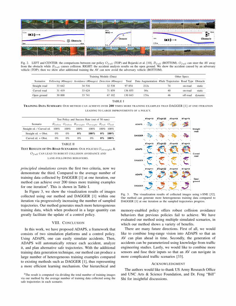
Fig. 2. LEFT and CENTER: the comparisons between our policy Ofull (TOP) and Bojarski et al. [10], Bfull (BOTTOM). Ofull can steer the AV awayfrom the obstacle while Bfull causes collision. RIGHT: the accident analysis results on the open ground. We show the accident caused by an adversaryvehicle (TOP); then we show after additional training the AV can now avoid the adversary vehicle (BOTTOM).

Training Module (Data) Other Specs

Scenarios Following (#Images) Avoidance (#Images) Detection (#Images) Total Data Augmentation #Safe Trajectories Road Type Obstacle

Straight road 33 642 34 516 32 538 97 854 212x 74 on-road static

Curved road 31 419 33 624 71 859 136 855 98x 40 on-road static

Open ground 30 000 33 741 67 102 130 843 178x 46 off-road dynamic

TABLE ITRAINING DATA SUMMARY: OUR METHOD CAN ACHIEVE OVER 200 TIMES MORE TRAINING EXAMPLES THAN DAGGER [1] AT ONE ITERATION

LEADING TO LARGE IMPROVEMENTS OF A POLICY.

Test Policy and Success Rate (out of 50 runs)

Scenario Bfollow Ofollow Bstraight Ostraight Bfull Ofull

Straight rd. / Curved rd. 100% 100% 100% 100% 100% 100%

Straight rd. + Obst. 0% 0% 0% 100% 0% 100%

Curved rd. + Obst. 0% 0% 0% 0% 0% 100%

TABLE IITEST RESULTS OF ON-ROAD SCENARIOS: OUR POLICIES Ostraight &

Ofull CAN LEAD TO ROBUST COLLISION AVOIDANCE AND

LANE-FOLLOWING BEHAVIORS.

principled simulations covers the first two criteria, now wedemonstrate the third. Compared to the average number oftraining data collected by DAGGER [1] at one iteration, ourmethod can achieve over 200 times more training examplesfor one iteration4. This is shown in Table I.

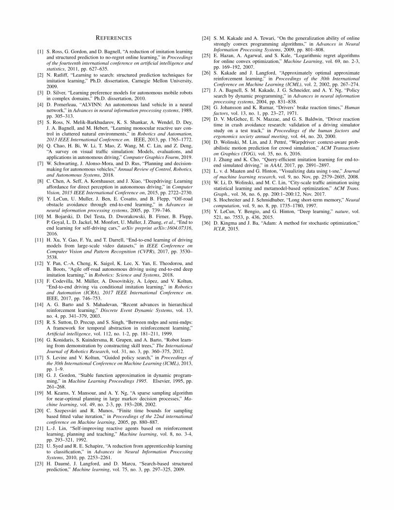
In Figure 3, we show the visualization results of imagescollected using our method and DAGGER [1] within oneiteration via progressively increasing the number of sampledtrajectories. Our method generates much more heterogeneoustraining data, which when produced in a large quantity cangreatly facilitate the update of a control policy.

VIII. CONCLUSION

In this work, we have proposed ADAPS, a framework thatconsists of two simulation platforms and a control policy.Using ADAPS, one can easily simulate accidents. Then,ADAPS will automatically retrace each accident, analyzeit, and plan alternative safe trajectories. With the additionaltraining data generation technique, our method can produce alarge number of heterogeneous training examples comparedto existing methods such as DAGGER [1], thus representinga more efficient learning mechanism. Our hierarchical and

4The result is computed via dividing the total number of training imagesvia our method by the average number of training data collected using thesafe trajectories in each scenario.

Fig. 3. The visualization results of collected images using t-SNE [32].Our method can generate more heterogeneous training data compared toDAGGER [1] at one iteration as the sampled trajectories progress.

memory-enabled policy offers robust collision avoidancebehaviors that previous policies fail to achieve. We haveevaluated our method using multiple simulated scenarios, inwhich our method shows a variety of benefits.

There are many future directions. First of all, we wouldlike to combine long-range vision into ADAPS so that anAV can plan ahead in time. Secondly, the generation ofaccidents can be parameterized using knowledge from trafficengineering studies. Lastly, we would like to combine moresensors and fuse their inputs so that an AV can navigate inmore complicated traffic scenarios [33].

ACKNOWLEDGMENT

The authors would like to thank US Army Research Officeand UNC Arts & Science Foundation, and Dr. Feng “Bill”Shi for insightful discussions.

REFERENCES

[1] S. Ross, G. Gordon, and D. Bagnell, “A reduction of imitation learningand structured prediction to no-regret online learning,” in Proceedingsof the fourteenth international conference on artificial intelligence andstatistics, 2011, pp. 627–635.

[2] N. Ratliff, “Learning to search: structured prediction techniques forimitation learning,” Ph.D. dissertation, Carnegie Mellon University,2009.

[3] D. Silver, “Learning preference models for autonomous mobile robotsin complex domains,” Ph.D. dissertation, 2010.

[4] D. Pomerleau, “ALVINN: An autonomous land vehicle in a neuralnetwork,” in Advances in neural information processing systems, 1989,pp. 305–313.

[5] S. Ross, N. Melik-Barkhudarov, K. S. Shankar, A. Wendel, D. Dey,J. A. Bagnell, and M. Hebert, “Learning monocular reactive uav con-trol in cluttered natural environments,” in Robotics and Automation,2013 IEEE International Conference on. IEEE, 2013, pp. 1765–1772.

[6] Q. Chao, H. Bi, W. Li, T. Mao, Z. Wang, M. C. Lin, and Z. Deng,“A survey on visual traffic simulation: Models, evaluations, andapplications in autonomous driving,” Computer Graphics Fourm, 2019.

[7] W. Schwarting, J. Alonso-Mora, and D. Rus, “Planning and decision-making for autonomous vehicles,” Annual Review of Control, Robotics,and Autonomous Systems, 2018.

[8] C. Chen, A. Seff, A. Kornhauser, and J. Xiao, “Deepdriving: Learningaffordance for direct perception in autonomous driving,” in ComputerVision, 2015 IEEE International Conference on, 2015, pp. 2722–2730.

[9] Y. LeCun, U. Muller, J. Ben, E. Cosatto, and B. Flepp, “Off-roadobstacle avoidance through end-to-end learning,” in Advances inneural information processing systems, 2005, pp. 739–746.

[10] M. Bojarski, D. Del Testa, D. Dworakowski, B. Firner, B. Flepp,P. Goyal, L. D. Jackel, M. Monfort, U. Muller, J. Zhang, et al., “End toend learning for self-driving cars,” arXiv preprint arXiv:1604.07316,2016.

[11] H. Xu, Y. Gao, F. Yu, and T. Darrell, “End-to-end learning of drivingmodels from large-scale video datasets,” in IEEE Conference onComputer Vision and Pattern Recognition (CVPR), 2017, pp. 3530–3538.

[12] Y. Pan, C.-A. Cheng, K. Saigol, K. Lee, X. Yan, E. Theodorou, andB. Boots, “Agile off-road autonomous driving using end-to-end deepimitation learning,” in Robotics: Science and Systems, 2018.

[13] F. Codevilla, M. Muller, A. Dosovitskiy, A. Lopez, and V. Koltun,“End-to-end driving via conditional imitation learning,” in Roboticsand Automation (ICRA), 2017 IEEE International Conference on.IEEE, 2017, pp. 746–753.

[14] A. G. Barto and S. Mahadevan, “Recent advances in hierarchicalreinforcement learning,” Discrete Event Dynamic Systems, vol. 13,no. 4, pp. 341–379, 2003.

[15] R. S. Sutton, D. Precup, and S. Singh, “Between mdps and semi-mdps:A framework for temporal abstraction in reinforcement learning,”Artificial intelligence, vol. 112, no. 1-2, pp. 181–211, 1999.

[16] G. Konidaris, S. Kuindersma, R. Grupen, and A. Barto, “Robot learn-ing from demonstration by constructing skill trees,” The InternationalJournal of Robotics Research, vol. 31, no. 3, pp. 360–375, 2012.

[17] S. Levine and V. Koltun, “Guided policy search,” in Proceedings ofthe 30th International Conference on Machine Learning (ICML), 2013,pp. 1–9.

[18] G. J. Gordon, “Stable function approximation in dynamic program-ming,” in Machine Learning Proceedings 1995. Elsevier, 1995, pp.261–268.

[19] M. Kearns, Y. Mansour, and A. Y. Ng, “A sparse sampling algorithmfor near-optimal planning in large markov decision processes,” Ma-chine learning, vol. 49, no. 2-3, pp. 193–208, 2002.

[20] C. Szepesvari and R. Munos, “Finite time bounds for samplingbased fitted value iteration,” in Proceedings of the 22nd internationalconference on Machine learning, 2005, pp. 880–887.

[21] L.-J. Lin, “Self-improving reactive agents based on reinforcementlearning, planning and teaching,” Machine learning, vol. 8, no. 3-4,pp. 293–321, 1992.

[22] U. Syed and R. E. Schapire, “A reduction from apprenticeship learningto classification,” in Advances in Neural Information ProcessingSystems, 2010, pp. 2253–2261.

[23] H. Daume, J. Langford, and D. Marcu, “Search-based structuredprediction,” Machine learning, vol. 75, no. 3, pp. 297–325, 2009.

[24] S. M. Kakade and A. Tewari, “On the generalization ability of onlinestrongly convex programming algorithms,” in Advances in NeuralInformation Processing Systems, 2009, pp. 801–808.

[25] E. Hazan, A. Agarwal, and S. Kale, “Logarithmic regret algorithmsfor online convex optimization,” Machine Learning, vol. 69, no. 2-3,pp. 169–192, 2007.

[26] S. Kakade and J. Langford, “Approximately optimal approximatereinforcement learning,” in Proceedings of the 30th InternationalConference on Machine Learning (ICML), vol. 2, 2002, pp. 267–274.

[27] J. A. Bagnell, S. M. Kakade, J. G. Schneider, and A. Y. Ng, “Policysearch by dynamic programming,” in Advances in neural informationprocessing systems, 2004, pp. 831–838.

[28] G. Johansson and K. Rumar, “Drivers’ brake reaction times,” Humanfactors, vol. 13, no. 1, pp. 23–27, 1971.

[29] D. V. McGehee, E. N. Mazzae, and G. S. Baldwin, “Driver reactiontime in crash avoidance research: validation of a driving simulatorstudy on a test track,” in Proceedings of the human factors andergonomics society annual meeting, vol. 44, no. 20, 2000.

[30] D. Wolinski, M. Lin, and J. Pettre, “Warpdriver: context-aware prob-abilistic motion prediction for crowd simulation,” ACM Transactionson Graphics (TOG), vol. 35, no. 6, 2016.

[31] J. Zhang and K. Cho, “Query-efficient imitation learning for end-to-end simulated driving,” in AAAI, 2017, pp. 2891–2897.

[32] L. v. d. Maaten and G. Hinton, “Visualizing data using t-sne,” Journalof machine learning research, vol. 9, no. Nov, pp. 2579–2605, 2008.

[33] W. Li, D. Wolinski, and M. C. Lin, “City-scale traffic animation usingstatistical learning and metamodel-based optimization,” ACM Trans.Graph., vol. 36, no. 6, pp. 200:1–200:12, Nov. 2017.

[34] S. Hochreiter and J. Schmidhuber, “Long short-term memory,” Neuralcomputation, vol. 9, no. 8, pp. 1735–1780, 1997.

[35] Y. LeCun, Y. Bengio, and G. Hinton, “Deep learning,” nature, vol.521, no. 7553, p. 436, 2015.

[36] D. Kingma and J. Ba, “Adam: A method for stochastic optimization,”ICLR, 2015.

IX. APPENDIX

A. Solving An SPC Task

We show the proofs of solving an SPC task using standardsupervised learning, DAGGER [1], and ADAPS, respec-tively. We use “state” and ”observation” interchangeablyhere as for these proofs we can always find a deterministicfunction to map the two.

1) Supervised Learning: The following proof is adaptedand simplified from Ross et al. [1]. We include it here forcompleteness.

Theorem 2: Consider a T -step control task. Let ε =Eφ∼dπ∗ ,a∗∼π∗(φ) [l (φ, π, a∗)] be the observed surrogate lossunder the training distribution induced by the expert’s policyπ∗. We assume C ∈ [0, Cmax] and l upper bounds the 0-1loss. J (π) and J (π∗) denote the cost-to-go over T stepsof executing π and π∗, respectively. Then, we have thefollowing result:

J (π) ≤ J (π∗) + CmaxT2ε.

Proof: In order to prove this theorem, we introduce thefollowing notation and definitions:

• dπt,c: the state distribution at t as a result of the followingevent: π is executed and has been choosing the sameactions as π∗ from time 1 to t− 1.

• pt−1 ∈ [0, 1]: the probability that the above-mentionedevent holds true.

• dπt,e: the state distribution at t as a result of the followingevent: π is executed and has chosen at least one differentaction than π∗ from time 1 to t− 1.

• (1 − pt−1) ∈ [0, 1]: the probability that the above-mentioned event holds true.

• dπt = pt−1dπt,c + (1− pt−1)dπt,e: the state distribution at

t.• εt,c: the probability that π chooses a different action

than π∗ in dπt,c.• εt,e: the probability that π chooses a different action

than π∗ in dπt,e.• εt = pt−1εt,c + (1 − pt−1)εt,e: the probability that π

chooses a different action than π∗ in dπt .• Ct,c: the expected immediate cost of executing π in dπt,c.• Ct,e: the expected immediate cost of executing π in dπt,e.• Ct = pt−1Ct,c+(1−pt−1)Ct,e: the expected immediate

cost of executing π in dπt .• C∗t,c: the expected immediate cost of executing π∗ indπt,c.

• Cmax: the upper bound of an expected immediate cost.• J (π) =

∑Tt=1 Ct: the cost-to-go of executing π for T

steps.• J (π∗) =

∑Tt=1 C

∗t,c: the cost-to-go of executing π∗ for

T steps.

The probability that the learner chooses at least one differentaction than the expert in the first t steps is:

(1− pt) = (1− pt−1) + pt−1εt,c.

This gives us (1− pt) ≤ (1− pt−1) + εt since pt−1 ∈ [0, 1].Solving this recurrence we arrive at:

1− pt ≤t∑i=1

εi.

Now consider in state distribution dπt,c, if π chooses adifferent action than π∗ with probability εt,c, then π willincur a cost at most Cmax more than π∗. This can berepresented as:

Ct,c ≤ C∗t,c + εt,cCmax.

Thus, we have:

Ct = pt−1Ct,c + (1− pt−1)Ct,e

≤ pt−1C∗t,c + pt−1εt,cCmax + (1− pt−1)Cmax

= pt−1C∗t,c + (1− pt)Cmax

≤ C∗t,c + (1− pt)Cmax

≤ C∗t,c + Cmax

t∑i=1

εi.

We sum the above result over T steps and use the fact1T

∑Tt=1 εt ≤ ε:

J (π) ≤ J (π∗) + Cmax

T∑t=1

t∑i=1

εi

= J (π∗) + Cmax

T∑t=1

(T + 1− t)εt

≤ J (π∗) + CmaxT

T∑t=1

εt

≤ J (π∗) + CmaxT2ε.

2) DAGGER: The following proof is adapted from Rosset al. [1]. We include it here for completeness. Note that forTheorem 3, we have arrived at the different third term as ofRoss et al. [1].

Lemma 1: [1] Let P and Q be any two distributions overelements x ∈ X and f : X → R, any bounded function suchthat f(x) ∈ [a, b] for all x ∈ X . Let the range r = b − a.Then |Ex∼P [f(x)]− Ex∼Q [f(x)] | ≤ r

2‖P −Q‖1.Proof:

|Ex∼P [f(x)]− Ex∼Q [f(x)] |

= |∫x

P (x)f(x)dx−∫x

Q(x)f(x)dx|

= |∫x

f(x) (P (x)−Q(x)) dx|

= |∫x

(f(x)− c) (P (x)−Q(x)) dx|,∀c ∈ R

≤∫x

|f(x)− c||P (x)−Q(x)|dx

≤ maxx|f(x)− c|

∫x

|P (x)−Q(x)|dx

= maxx|f(x)− c|‖P −Q‖1.

Taking c = a+ r2 leads to maxx |f(x)− c| ≤ r

2 and provesthe lemma.

Lemma 2: [1] Let πi be the learned policy, π∗ be theexpert’s policy, and πi be the policy used to collect trainingdata with probability βi executing π∗ and probability 1−βiexecuting πi over T steps. Then, we have ‖dπi − dπi‖1 ≤2 min(1, Tβi).

Proof: In contrast to dπi which is the state distributionas the result of solely executing πi, we denote d as thestate distribution as the result of πi executing π∗ at leastonce over T steps. This gives us dπi = (1 − βi)

T dπi +(1− (1− βi)T

)d. We also have the facts that for any two

distributions P and Q, ‖P − Q‖1 ≤ 2 and (1 − β)T ≥1 − βT, ∀β ∈ [0, 1]. Then, we have ‖dπi − dπi‖1 ≤ 2 andcan further show:

‖dπi − dπi‖1 =(1− (1− βi)T

)‖d− dπi‖1

≤ 2(1− (1− βi)T

)≤ 2Tβi.

Theorem 3: [1] If the surrogate loss l ∈ [0, lmax] is thesame as the cost function C or upper bounds it, then afterN iterations of DAGGER:

J (π) ≤ J (π) ≤ Tεmin + Tεregret +O(f(T, lmax)

N). (5)

Proof: Let li (π) = Eφ∼dπi ,a∗∼π∗(φ) [l (φ, π, a∗)]] bethe expected loss of any policy π ∈ Π under the statedistribution induced by the learned policy πi at the ithiteration and εmin = minπ∈Π

1N

∑Ni=1 li(π) be the minimal

loss in hindsight after N ≥ i iterations. Then, εregret =1N

∑Ni=1 li(πi) − εmin is the average regret of this online

learning program. In addition, we denote the expected lossof any policy π ∈ Π under its own induced state distributionas L (π) = Eφ∼dπ,a∗∼π∗(φ) [l (φ, π, a∗)]] and consider π asthe mixed policy that samples the policies {πi}Ni=1 uniformlyat the beginning of each trajectory. Using Lemma 1 andLemma 2, we can show:

L(πi) = Eφ∼dπi ,a∗∼π∗(φ) [l (φ, πi, a∗)]

≤ Eφ∼dπi ,a∗∼π∗(φ) [l (φ, πi, a∗)] +

lmax2‖dπi − dπi‖1

≤ Eφ∼dπi ,a∗∼π∗(φ) [l (φ, πi, a∗)] + lmax min (1, Tβi)

= li (πi) + lmax min (1, Tβi) .

By further assuming βi is monotonically decreasing andnβ = arg maxn(βn >

1T ), n ≤ N , we have the following:

mini∈1:N

L(πi) ≤ L(π)

=1

N

N∑i=1

L(πi)

≤ 1

N

N∑i=1

li(πi) +lmaxN

N∑i=1

min (1, Tβi)

= εmin + εregret +lmaxN

nβ + T

N∑i=nβ+1

βi

.Summing over T gives us:

J(π) ≤ Tεmin + Tεregret +T lmaxN

nβ + T

N∑i=nβ+1

βi

.Define βi = (1− α)i−1, in order to have βi ≤ 1

T , we need(1−α)i−1 ≤ 1

T which gives us i ≤ 1+log 1

T

log (1−α) . In addition,

note now i = nβ and∑Ni=nβ+1 βi = (1−α)nβ−(1−α)N

α ≤1Tα , continuing the above derivation, we have:

J (π) ≤ Tεmin+Tεregret+T lmaxN

(1 +

log 1T

log (1− α)+

1

α

).

Given the fact J (π) = mini∈1:N J(πi) ≤ J(π) and repre-senting the third term as O( f(T,lmax)

N ), we have proved thetheorem.

3) ADAPS: With the assumption that we can treat thegenerated trajectories from our model and the additionaldata generated based on them as running a learned policyto sample independent expert trajectories at different stateswhile performing policy roll-out, we have the followingguarantee of ADAPS. To better understand the followingtheorem and proof, we recommend interested readers to readthe proofs of Theorem 2 and 3 first.

Theorem 4: If the surrogate loss l upper bounds the truecost C, by collecting K trajectories using ADAPS at eachiteration, with probability at least 1−µ, µ ∈ (0, 1), we havethe following guarantee:

J (π) ≤ J (π) ≤ T εmin+T εregret+O

T lmax√

log 1µ

KN

.

Proof: Assuming at the ith iteration, our model gener-ates K trajectories. These trajectories are independent fromeach other since they are generated using different parametersand at different states during the analysis of an accident.For the kth trajectory, k ∈ [[1,K]], we can construct anestimate lik(πi) = 1

T

∑Tt=1 li (φikt, πi, a

∗ikt), where πi is

the learned policy from data gathered in previous i − 1iterations. Then, the approximated expected loss li is theaverage of these K estimates: li(πi) = 1

K

∑Kk=1 lik(πi). We

denote εmin = minπ∈Π1N

∑Ni=1 li(π) as the approximated

minimal loss in hindsight after N iterations, then εregret =1N

∑Ni=1 li(πi)− εmin is the approximated average regret.

Let Yi,k = li(πi) − lik(πi) and define random vari-ables XnK+m =

∑ni=1

∑Kk=1 Yi,k +

∑mk=1 Yn+1,k, for

n ∈ [[0, N − 1]] and m ∈ [[1,K]]. Consequently, {Xi}NKi=1

form a martingale and |Xi+1 − Xi| ≤ lmax. By Azuma-Hoeffding’s inequality, with probability at least 1 − µ, we

have 1KNXKN ≤ lmax

√2 log 1

µ

KN .Next, we denote the expected loss of any policy π ∈

Π under its own induced state distribution as L (π) =Eφ∼dπ,a∗∼π∗(φ) [l (φ, π, a∗)]] and consider π as the mixedpolicy that samples the policies {πi}Ni=1 uniformly at thebeginning of each trajectory. At each iteration, during thedata collection, we only execute the learned policy instead ofmix it with the expert’s policy, which leads to L(πi) = l(πi).Finally, we can show:

mini∈1:N

L(πi) ≤ L(π)

=1

N

N∑i=1

L(πi)

=1

N

N∑i=1

li(πi)

=1

KN

N∑i=1

K∑k=1

(lik(πi) + Yi,k

)=

1

KN

N∑i=1

K∑k=1

lik(πi) +1

KNXKN

=1

N

N∑i=1

l(πi) +1

KNXKN

≤ 1

N

N∑i=1

l(πi) + lmax

√2 log 1

µ

KN

= εmin + εregret + lmax

√2 log 1

µ

KN.

Summing over T proves the theorem.

B. Network Specification

All modules within our control mechanism share a sim-ilar network architecture that combines Long Short-TermMemory (LSTM) [34] and Convolutional Neural Networks(CNN) [35]. Each image will first go through a CNN andthen be combined with other images to form a trainingsample to go through a LSTM. The number of images ofa training sample is empirically set to 5. We use the many-to-many mode of LSTM and set the number of hidden unitsof the LSTM to 100. The output is the average value of theoutput sequence.

The CNN consists of eight layers. The first five areconvolutional layers and the last three are dense layers. Thekernel size is 5×5 in the first three convolutional layers and3 × 3 in the other two convolutional layers. The first three

Fig. 4. Plotted collision-free trajectories generated by the expert algorithmfor a vehicle traveling on the right lane of a straight road, with an obstaclein front. Spans 74 trajectories from the first moment the vehicle perceivesthe obstacle (green, progressive avoidance) to the last moment the collisioncan be avoided (red, sharp avoidance).

convolutional layers have a stride of two while the last twoconvolutional layers are non-strided. The filters for the fiveconvolutional layers are 24, 36, 48, 64, 64, respectively. Allconvolutional layers use VALID padding. The three denselayers have 100, 50, and 10 units, respectively. We use ELUas the activation function and L2 as the kernel regularizerset to 0.001 for all layers.

We train our model using Adam [36] with initial learningrate set to 0.0001. The batch size is 128 and the number ofepochs is 500. For training Detection (a classification task),we use Softmax for generating the output and categoricalcross entropy as the loss function. For training Followingand Avoidance (regression tasks), we use mean squared error(MSE) as the loss function. We have also adopted cross-validation with 90/10 split. The input image data have 220×66 resolution in RGB channels.

C. Example Expert Trajectories

Figure 4 shows a set of generated trajectories for asituation where the vehicle had collided with a static obstaclein front of it after driving on a straight road. As expected,the trajectories feature sharper turns (red trajectories) as thestarting state tends towards the last moment that the vehiclecan still avoid the obstacle.

D. Learning From Accidents

For the following paragraph, we abusively note sk.x, sk.ythe position coordinates at state sk, and sk.vx, sk.vy thevelocity vector coordinates at state sk. Then, for any statesk ∈ {skf , ..., ska} we can define a line L(sk) = {lu =(sk.x, sk.y) + u × (−sk.vy, sk.vx) | u ∈ R}. On this line,we note li the furthest point on L(sk) from (sk.x, sk.y)which is at an intersection between L(sk) and a collision-free trajectory from solve(S). This point determines howfar the vehicle can be expected to stray from the originaltrajectory S before the accident, if it followed an arbitrarytrajectory from solve(S). We also note lrl and lrr the twointersections between L(sk) and the road edges (lrl is on the“left” with rl > 0, and lrr is on the “right” with rr < 0).These two points delimit how far from the original trajectory

Fig. 5. (This figure is copied from the main text to here for completeness.)Illustration of important points and DANGER/SAFE labels from Section VIfor a vehicle traveling on the right lane of a straight road, with an obstaclein front. Labels are shown for four points {lu1, lu2, lu3, lu4} illustratingthe four possible cases.

the vehicle could be. Finally, we define a user-set margin gas outlined below (we set g = 0.5 m).

Altogether, these points and margin are the limits of theregion along the original trajectory wherein we generateimages for training: a point lu ∈ L(sk) is inside the region ifit is between the original trajectory and the furthest collision-free trajectory plus a margin g (if lu and li are on the sameside, i.e. sign(u) = sign(i)), or if it is between the originaltrajectory and either road boundary plus a margin g (if luand li are not on the same side, i.e. sign(u) 6= sign(i)).

In addition, if a point lu ∈ L(sk) is positioned be-tween two collision-free trajectories Sk1 , Sk2 ∈ solve(S),we consider the two closest states on Sk1 , and the twoclosest states from Sk1 , and bi-linearly interpolate these fourstates’ velocity vectors, resulting in an approximate velocityvector vbilin(lu) at lu. Similarly, if a point lu ∈ L(sk) isnot positioned between two collision-free trajectories, weconsider the two closest states on the single closest collision-free trajectory Sk1 ∈ solve(S), and linearly interpolate theirvelocity vectors, resulting in an approximate velocity vectorvlin(lu) at lu.

From here, we can construct images at various points lualong L(sk) (increasing u by steps of 0.1 m), with variousorientation vectors (noted vu and within 2.5 degrees of(sk.vx, sk.vy)), and label them using the following scheme(also illustrated in Figure 5). If the expert algorithm madethe vehicle avoid obstacles by steering left (li with i > 0),there are four cases to consider when building a point lu:• u < i + g and u > i: lu is outside of the computed

collision-free trajectories solve(S), on the outside ofthe steering computed by the expert algorithm. Thelabel is SAFE if det(vlin(lu),vu) ≥ 0, and DANGERotherwise.

• u < i and u > 0: lu is inside the computedcollision-free trajectories solve(S). The label is SAFEif det(vbilin(lu),vu) ≥ 0 (over-steering), and DAN-GER otherwise (under-steering).

• u < 0 and u > rr: lu is outside the computed collision-free trajectories solve(S) on the inside of the steeringcomputed by the expert algorithm. The label is alwaysDANGER.

• u < rr and u > rr− g: lu is in an unattainable region,but we include it to prevent false reactions to similar(but safe) future situations. The label is DANGER ifdet(vlin(lu),vu) > 0, SAFE otherwise.

Here, the function det(·, ·) computes the determinant of twovectors from R2.

Conversely, if the expert algorithm made the vehicle avoidobstacles by steering right (li with i < 0), there are four casesto consider when building a point lu:• u > i − g and u < i: the label is SAFE ifdet(vlin(lu),vu) ≤ 0, and DANGER otherwise.

• u > i and u < 0: the label is SAFE ifdet(vbilin(lu),vu) ≤ 0, and DANGER otherwise.

• u > 0 and u < rl: the label is always DANGER.• u > rl and u < rl + g: the label is DANGER ifdet(vlin(lu),vu) < 0, SAFE otherwise.

We then generate images from these (position, orientation,label) triplets which are used to further train the Detectionmodule of our policy.

E. Experiment Setup

1) Scenarios: We have tested our method in three sce-narios. The first is a straight road which represents a lineargeometry, the second is a curved road which represents anon-linear geometry, and the third is an open ground. Thefirst two represent on-road situations while the last representsan off-road situation.

Both the straight and curved roads consist of two lanes.The width of each lane is 3.75 m and there is a 3 m shoulderon each side of the road. The curved road is half circularwith radius at 50 m and is attached to two straight roadsat each end. The open scenario is a 1000 m × 1000 mground, which has a green sphere treated as the target forthe Following module to steer the AV.

2) Vehicle Specs: The vehicle’s speed is set to 20 m/s,which value is used to compute the throttle value in thesimulator. Due to factors such as the rendering complexityand the delay of the communication module, the actualrunning speed is in the range of 20±1 m/s. The length andwidth of the vehicle are 4.5 m and 2.5 m, respectively. Thedistance between the rear axis and the rear of the vehicle is0.75 m. The front wheels can turn up to 25 degrees in eitherdirection. We have three front-facing cameras set behind themain windshield, which are at 1.2 m height and 1 m front tothe center of the vehicle. The two side cameras (one at leftand one at right) are set to be 0.8 m away from the vehicle’scenter axis. These two cameras are only used to capture datafor training Following. During runtime, our control policyonly requires images from the center camera to operate.

3) Obstacles: For the on-road scenarios, we use a scaledversion of a virtual traffic cone as the obstacle on both thestraight and curved roads. This scaling operation is meant topreserve the obstacle’s visibility, since at distances greaterthan 30m a normal-sized obstacle is quickly reduced to just afew pixels. This is an intrinsic limitation of the single-camerasetup (and its resolution), but in reality we can emulate this“scaling” using the camera’s zoom function for instance.

For the off-road scenario, we use a vehicle with the samespecifications as of the AV as the dynamic obstacle. Thisvehicle is scripted to collide into the AV on its default coursewhen no avoidance behavior is applied by the AV.

4) Training Data: In order to train Following, we havebuilt a waypoint system on the straight road and curved roadfor the AV to follow, respectively. By running the vehiclefor roughly equal distances on both roads, we have gatheredin total 65 061 images (33 642 images for the straight roadand 31 419 images for the curved road). On the open ground,we have sampled 30 000 positions and computed the angledifference between the direction towards the sphere targetand the forward direction. This gives us 30 000 trainingexamples.

In order to train Avoidance, on the straight road, we rewindthe accident by 74 frames starting from the frame that theaccident takes place, which gives us 74 safe trajectories.On the curved road, we rewind the accident by 40 framesresulting in 40 safe trajectories. On the open ground, werewind the accident by 46 frames resulting in 46 safetrajectories. By positioning the vehicle on these trajectoriesand capturing the image from the front-facing camera, wehave collected 34 516 images for the straight road, 33 624images for the curved road, and 33 741 images for the openground.

For the training of Detection, using the mechanism ex-plained in Subsection VI-B, we have collected 32 538 imagesfor the straight road, 71 859 for the curved road, and 67 102images for the open ground.