ad-aiob 802 army missil coma redstion arsenal al guidance ... · ad-aiob 802 army missil coma...
TRANSCRIPT

AD-AIOB 802 ARMY MISSIL COMA REDSTION ARSENAL AL GUIDANCE A--ETC F/6 19/2OJ[ITAL COIUTER 1MENTATIOM OF A DISCRETE.TIME OZSTURBANCE---ETC(U)
7 AD-A105~
JU 80 y MI SL COMA$
RESON E R
UNCLASSIFIED DRSMV/RG-80-27 TR S 'IE-AO-E9SO L58 NL,2 1111111 1rmmmmmu ***l
[.mmhhMhhl .ME-mom
IIIIIIIIIEILIIIIIIIIII

-3"94

... .- ~ .__._.__._y

SECURITY CLASSIFICATION OF THIS PAGE (Whon bet. Ent...d)
REPORT DOCUMAENTATION PAGE BFRE COMP~cLTN ORMI. REPORT NUMBER 12. 90VT ACCESSION NO. 3. RECIPIENT-S CATALOG NUMBER
TR-RG-80-27 A A -16 S-g I4. TITLE (and S.bett1) S. TYPE Of REPORT A PERIOD COVERED
Digital Computer Implementation of a Discrete-Time Disturbance-Accommodating Controller (DAC) Technical ReportFor a General First-Order Plant with First-Order 6. PERFORMING ORG. REPORT NUNGER
Disturbance7. AUTNOR(e) S. CONTRACT OR GRANT NUMBER(*)
Larmon S. Isom9. PERFORMING ORGANIZATION NAME AND ADDRESS 10. PROGRAM4 ELEMENT, PROJECT. TASK
AREA & WORK UNIT NUMMER$Commander, US Army Missile Command .ATTN: DRSMI-RGRedstone Arsenal, Alabama 35898 .
It. CONTROLLING OFFICE NAME AND ADDRESS 12. REPORT DATE
Commander, US Army Missile Command June 1980 -
ATTN: DRSMI-RPT 1S. NUMBER OF PAGES'
Redstone Arsenal, Alabama 3589814. MONITORING AGENCY NAME & AOORCSS(if differt &om CmvwIS1n* 0111..) 1S. SECURITY CLASS. (of bV*S repot)
UNCLASSI FIEDIS* DEC hICATION/DOWNGRADING
IA. DISTRhBUTION STATEMENT (*I &is eport)
Approved for public release; distribution unlimited.
17. DISTRIBUTION STATEMENT (of Me abeit eteremtd in Stock 2O. it dithretmIb Report)
W. SUPPsMUTARY MOVES
IS. KEY WORDS (ofakwo a rees MV.4 of., u...ewy OWd I~AV w~t me" ".a uim)
discrete controllersauto p1lotsregulatorsdisturbance-accommodating controldigital control
20. A.STUAc? ' tbmu40 foars SI11 If .e..uoiny 411 I~f OF stock
Results are presented which demonstrate the performance of a discretecontroller with disturbance-absorbing capability. The design approach isexplained and the implementation of the design on a PDP 11/34 computer isdocumented, along with performance plots showing results with several types ofdisturbances. Applications of this approach include pointing and trackingproblems, missile autopilots, and isolation of guns mounted on helicopters.
AN 31S 0 STGO O SSMLT Un clas s if iedol ~SECUIT CLAGNIFfCATO OF TIlS PAGIE (111be Des E.,I.eo

FOREWORD
Shortly after submitting this report for publication, Larmon Isomdeparted this life. His years of' dedicated work in the Guidance andControl Directorate of the US Army Missile Command are fondly recalledand appreciated by his associates. This report documents his finaltask.
Acevnsslon For
NTIS (':--.SIPTT 7 TAB L
Av'illhAbilltv c)1
AVitI. raid/ar

TABLE OF CONTENTS
SECTION PAGE
I. INTRODUCTION .............. ........................... 5
II. DIGITAL COMPUTER IMPLEMENTATION ........ ................. 5
A. THE DAC DESIGN EXAMPLE .......... .................... 6B. THE PDP-11/34 PROGRAM(S) ....... ................... 10.oC. PROGRAM EXECUTION ......... ...................... 17
III. RESULTS OF EXECUTION ......... ....................... 17
IV. CONCLUSIONS ........... ........................... 35
BIBLIOGRAPHY

ILLUSTRATIONS
FIGURE PAGE
1 Organization and Block Diagram of Problem ..... ........... 72 Listing of the Main Program ...... .................. . 113 Listing Of Runga-Kutta Integration Routine .. .......... . 144 Listing of the Graphical Plot Program .... ............. . 155 Listing of Output Results from DAC Program 1 Execution, Case 1 216 Plot 1; DAC Program 1, Case 1 ..... ................. . 237 Plot 2; DAC Program 1, Case 1 ..... ................. . 248 Plot 3; DAC Program 1, Case 1 ..... ................. . 259 Plot 4; DAC Program 1, Case 1 ..... ................. . 26
10 Plot 5; DAC Program 1, Case 1 ..... ................. . 2711 Plot 6; DAC Program 1, Case 1 ..... ................. . 2812 Plot 7; DAC Program 1, Case 1 ........... ....... 2913 Plot 8; DAC Program 1, Case 1 ..... ................. . 3014 Plot 9; DAC Program 1, Case 1 ..... ................. . 3115 Plot 10; DAC Program 1, Case 1 ..... ................ . 3216 Plot 11; DAC Program 1, Case 1 ..... ................ . 3317 Plot 12; DAC Program 1, Case 1 ..... ................ . 3418 Output Listing (Condensed) of Results, Case 2 .......... . 3819 Plot 1; DAC Program 1, Case 2 ..... ................. . 3920 Plot 10; DAC Program 1, Case 2 ..... ................ . 4021 Plot 11; DAC Program 1, Case 2 ..... ................ . 4122 Output Listing (Condensed) of Results, Case 3 .......... .. 4223 Plot 1; DAC Program 1, Case 3 ..... ................. . 4324 Plot 10; DAC Program 1, Case 3 ..... ................ . 4425 Plot ll DAC Program 1, Case 3 ................ 4526 Output Listing (Condensed) of Results, Case 4 .......... .. 4627 Plot 1; DAC Program 1, Case 4 ..... ................. . 4728 Plot 10; DAC Program 1, Case 4 ..... ................ . 4829 Plot 11; DAC Program 1, Case 4 ..... ................ . 4930 Output Listing of Results, Case 10 .... .............. 5031 Plot 1; DAC Program 1, Case 10 ..... ................ . 5332 Plot 10; DAC Program 1, Case 10 ..... ................ . 5433 Plot 11; DAC Program 1, Case 10 ...... .... ... ....... 5534 Output Listing of Results, Case 20 .... .............. . 5635 Plot 1; DAC Program 1, Case 20 ..... ................ . 5936 Plot 2; DAC Program 1, Case 20 ..... ................ . 6037 Plot 3; DAC Program 1, Case 20 ..... ................ . 6138 Plot 4; DAC Program 1, Case 20 ..... ................ . 6239 Plot 5; DAC Program 1, Case 20 ..... ................ . 6340 Plot 6; DAC Program 1, Case 20 ..... ................ . 6441 Plot 7; DAC Program 1, Case 20 ..... ................ . 65
43 Plot 9; DAC Program 1, Case 20 ..... ................ . 6644 Plot 10; DAC Program 1, Case 20 ..... ................ . 6745 Plot 11; DAC Program 1, Case 20 ..... ................ . 6846 Output Listing (Condensed) of Results, Case 29 . ........ . 6947 Plot 1; DAC Program 1, Case 29 ..... ................ . 7048 Plot 10; DAC Program 1, Case 29 ..... ................ . 71
2

ILLUSTRATIONS (CONCLUDED)
FIGURE PAGE
49 Output Listing (Condensed) of Results, Case 31. ......... 7250 Plot 1; DAC Program 1, Case 31..................7351 Plot 2; DAC Program: 1, Case 31 .................. 7452 Plot 3; DAC Program 1, Case 31..................7553 Plot 4; DAC Program 1, Case 31..................7654 Plot 5; DAC Program 1, Case 31..................7755 Plot 6; DAC Program 1, Case 31..................7856 Plot 7; DAC Program 1, Case 31..................7957 Plot 8; DAC Program 1, Case 31..................8058 Plot 9; DAC Program 1, Case 31..................8159 Plot 10; DAC Program 1, Case 31............ ....... 8260 Output Listing (Condensed) of Results, Case 32...........8361 Plot 1; DAC Program 1, Case 32 .................. 8462 Plot 3; DAC Program 1, Case 32 .................. 8563 Plot 10; DAC Program 1, Case 32. ................. 8664 Plot 11; DAC Program 1, Case 32. ................. 8765 Output Listing of Results, Case 46................8866 Plot 1; DAC Program 1, Case 46 ................ 967 Plot 3; DAC Program 1, Case 46 .................. 9168 Plot 10; DAC Program 1, Case 46. ................. 9269 Plot 11; DAC Program 1, Case 46. ................. 93
3I

I I U I ~ I . ..
TABLES
TABLE PAGE
1 A Cross Index of Variables ......... ................... 92 Legend to the Graphical Plots ...... ................. .. 183 A Typical List of Task Creation Commands .... ............ . 194 A Typical List of Task Execution Commands ... ........... . 195 Graphical Plot Program Task Cieation Commands .. ......... . 206 Summary of DAC Program Implementation Execution Results
Contained in This Report ....... .................... . 36
4
14
'a.

I. INTRODUCTION
The US Army Missile Command (MICOM, is engaged in a research program to Fdevelop an advanced guidance and control system for future (1990's) Army
modular missiles. Principal investigators have defined several technical
areas in which government and contractor personnel are contributing to the
overall program objectives. One of these technical areas is the Disturbance
Accommodating Control (DAC) theory and the design of discrete-time disturbance-
accommodating controllers for discrete-time, sampled-data control problems.
The DAC method of design, using a combination of waveform-mode distrubance
modeling and state-variable control techniques, was developed by
Dr. C. D. Johnson of the University of Alabama in Huntsville. As a tool for
design of controllers, the DAC approach permits three primary modes of
distrubance accommodation: (1) cancellation (absorption) of disturbance
effects, (2) minimization of disturbance effects, or (3) constructive utiliza-
tion of the disturbances as an aid in accomplishing the primary control task.
These disturbance accommodations are realized in addition to the usual control
efforts required to satisfy system performance requirements without
disturbances.
This report describes the digital computer implementation and the results
obtained from the design of a discrete-time disturbance-accoumodating
controller. The digital computer implementation and the results presented in
this report were obtained by using the disturbance cancellation mode of the
discrete-time DAC design on a liniar, time-invariant plant. The controllers
obtained via this design method are termed diatuzbance abeovption controllers
for regulating the plant state to zero.
II. DIGITAL COMPUTER IMPLEMENTATION
This section of the report presents the details of the discrete-time DAC
program design method. The first section presents the equations of the total
system to be implemented. However, these equations may be considered to con-
sist of three groups: (1) continuous-tre disturbances, (2) continuous-time
plant (system), and (3) discrete-time DAC. The second section presents the
FORTRAN program implementation of this DAC design method for execution on the
PDP-11/34 digital computer.
5

A. THE DAC DESIGN EXAMPLE
The discrete-time DAC design program example to be considered is a
regulator problem that involves a first-order controlled plant acted upon by a
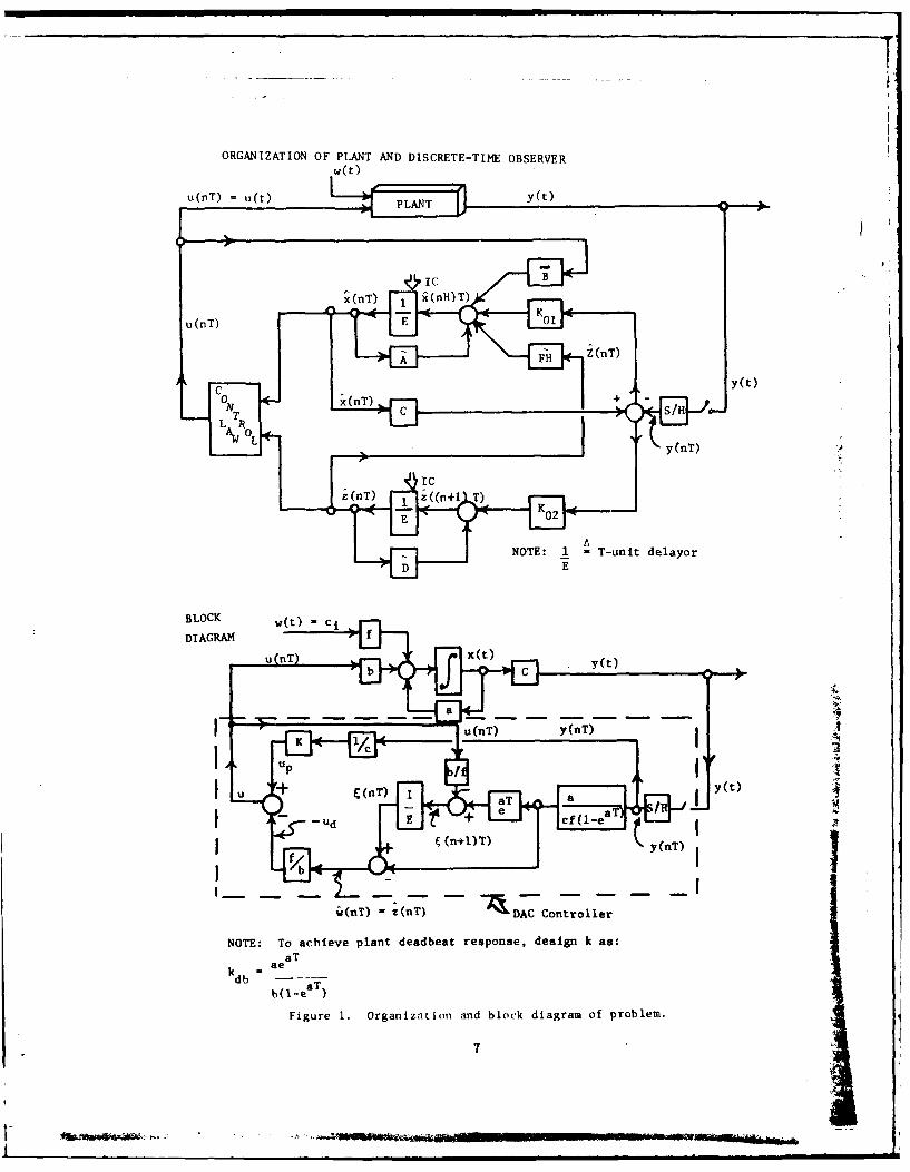
constant piecewise disturbance. The complete block diagram of the continuous-
time system (plant) with the continuous-time DAC design is as shown in
Figure 1. From the block diagram, the following equations may be immediately
written.
For the piecewise disturbance,
W(t) = c.e at (1)
For the first-order plant (system),
x(t) = a x(t) + b U(nT) + f w(t) (2)
x(t) ft (t) dt + x(o) (3)
y(t) = c x(t) (4)
For the discrete-time DAC controller design,
y(nT) = y(t) (5)
TMP1 [edT (a - d) y (nT)]/ of [(edT- eaT)] (6)
U = K y(nT)/c (7)
W(n) = [i E[f(n + 1)T] (8)
z (n) = (nT) - TMPl (9)
Ud = )af/[b(a- d)] f(edT -eaT )/eaT- 1 z(nT) (10)
U(nT) = U p+ Ud 11
l(a - d) e(a + d) (T )
&+n+lT [(d adeT (ea - (nT) (2eeT
6
... ...
ORGANIZATION OF PLANT AND DISCRETE-TIME OBSERVER
BLOCK
ICI
g(nT) - (n)T-) A onrle
(nT
k - aedbnT M
bPH- )~T
Figure~~ 1. Ognzain ad lc iarmo polm
C +

where K = db= aeaT/ b(l e a T (13)
E I a unit delayer (14)
Observe that there are three cases to be considered in the use of
Eqs. (6), (10), and (12). These three cases are as follows: (1) where d = 0,
(2) where d = a, and (3) where neither case (1) or (2) applies. These cases
are considered in the DAC program implementation by using the FORTRAN IF
statement.
Note that the disturbances w(t) have been experimentally modeled and
found to obey a first-order equation of
w(t) = z(t) (15)
z = dz + a(t) (16)
where the (real) coefficient d is assumed to be known. Now, the disturbance
model (given by Eq. (1)) is
atw(t) = c e (17)
where a is any arbitrary (real) scalar constant. This implies that
citz(t) = c.e (18)
z(t) = c.eat dz(t) (19)
Therefore, a = d, which may be obtained from these relationships as shown.
By setting d = 0, the case of constant disturbances is obtained; setting
d > 0 yields the case of exponentially growing disturbances; and setting d < 0
yields the case of exponentially decaying disturbances. Thus, this permits a
wide range of realistic disturbances to be utilized in the design process of
high performance digital controllers.
Also, the above equations have been written in the mathematical notation
of Reference 1 as utilized by Dr. Johnson. Table 1 is shown as an aid to
understanding the notation of the above equations and their usage in the
FORTRAN DAC program implementation; this implementation is described in the
next section.
8

TABLE 1. A CROSS INDEX OF VARIABLES
VALUE USEDMATHEMATICAL FORTRAN IN
SYMBOL SYMBOL CASE 1 MEANING AND/OR USAGE
A, a A 1.0 Coefficient of x(t)
AWT 0.0 Coefficient of e
B, b B 1.0 Coefficient of plant equation
C C 1.0 Coefficient of plant output
C. CWT 1.0 Coefficient of Cea
D D Calculated Sane as AWT
dt DT 1/64 Integration interval
f F 1.0 Coefficient of disturbance
ICN 1.0 Case number parameter
-- ITP 0.0 Print interval
K Calculated Equation (13)
-- KU'2TA Calculated Integration control parameter
-- NX 1.0 Number of variables to integrate
T ST 8 * DT Sample interval
t T 0.0 Time
-- TMP1 Calculated Equation (6)
-- TSTOP 1.0 Time to stop
Ud UD Calculated Equation (10)
U(nT) = U(t) UNT Calculated Equation (11)
U UP Calculated Equation (7)p
D(t) WT Calculated Equation (2)
x(t) XDT Calculated Equation (2)
[r(n + T)] XINPT Calculated Equation (12)
(nT) XINT Calculated Equation (8)
y (t) IT Calculated Equation (3)
y (nT) YNT Calculated Equation (5)y (t) YT Calculated Equation (4)
{(nT) ZHNT Calculated Equation (9)
-- V Calculated Array of graphical plot variables
1/E .... Used to denote a unit delayer
e E'P Natural logarithm as in Eq. (1)
9__inrnu~ahi ~{. ~*~- 4~-eA1 - - ____ ---.

B. THE PDP 11/34 PROGRAM(S)
This section of the report describes the digital computer implementation
of the first-order system (plant) with a constant piecewise disturbance and
the associated designed discrete-time DAC controller. These programs have
been programmed in the FORTRAN programming language for execution by a
PDP 11/34 digital computer and its operating system software. A listing of
the main program is as shown in Figure 2, which contains the equations given
in the previous section of the report for the constant piecewise disturbance
model, the first-order plant (system) model, and the discrete-time DAC
controller design model. Also contained in this listing are the equations and
necessary statements for the initial conditions, values of variable parameters,
and control of the program during execution.
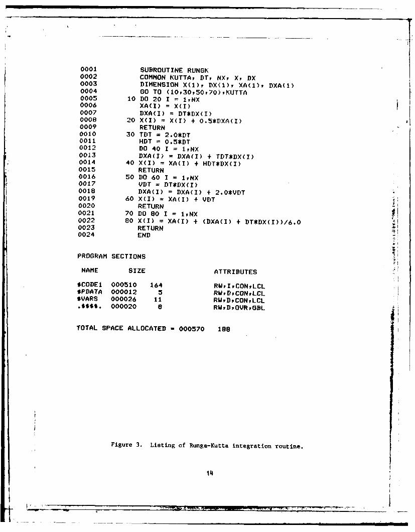
The required plant differential equations (one in this case) are
integrated by the fourth-order Runga-Kutta integration scheme as contained in
its listing shown in Figure 3. This very familiar and widely used integration
scheme is
Yn+l =Yn + (k 0 + 2k1
+ 2k2 + k3) (20)
where k0 = h • f Y (21)
k I = h f (xn + h, y + 2 k0 (22)
k = h . f (x+ h, y + k) (23)
3 =h *fx+h, Y1 +k2) (24)t
Table 1 is a cross index of the variables contained in the block diagram
(Figure 1 and the mathematical equations written from the block diagram) and
the FORTRAN program variable names contained in the listings of the designed
discrete-time DAC digital computer implementation. Also, Table 1 presents the
value of the variables as used in the execution of the DAC program for case 1.
The graphical plots of the dependent variables versus the independent
variable time for the designed DAC controller program were obtained by the
execution of the plot program as shown in the listing of Figure 4. A legend
10
I- _.___.__,____.

C ** DAC PROGRAM EXAMPLE NUMBER 1.C *** FIRST-ORDER SYSTEM WITH A CONSTANT DISTURBANCE.C ** UNSTABLE SYSYTEM
0001 REAL K0002 COMMON KUTTA, DT, NX, XT, XDT, YT 40003 DIMENSION V(12)0004 DATA A/1.0/0005 DATA B/1.0/0006 DATA C/1.0/0007 DATA F/10/0008 DATA UNT/00/0009 NX = 10010 T = 0.00011 *DT - 1.0/64.00012 TSTOP = 1.00013 ITP =00014 ST = 8.0*DT0015 XINPT = 0.00016 PRINT 10210017 PRINT 200018 READ(5,21) ICN0019 WRITE(2) ICN0020 PRINT 23
0021 READ(5,1040) XT0022 PRINT 800023 READ(5,1040) CWT0024 PRINT 810025 READ(5,1040) AWT
0026 D = AWT0027 PRINT 10200028 9 CONTINUE0029 DO 51 KUTTA = 1,40030 YT = C*XT0031 GO TO (60,50,30,40) KUTTA0032 60 CONTINUE0033 IF(MOD(ITP,8) .NE. 0) GO TO 620034 V(1) - XT0035 V(2) = YNT0036 V(3) - UNT0037 V(4) - UD0038 V(5) - UP0039 V(6) = XINT0040 V(7) = XINPT0041 V(8) - TNPI0042 V(9) = ZHNT0043 V(10) - XDT0044 V(11) - WT0045 V(12) - T0046 WRITE(2) V0047 K - A*EXP(A*ST)/(B*(1.0 - EXP(A*ST)))0048 )NT - YT
0049 IF(D *EO. 0.0) TMP1 = A*YNT/(C*F*(1.0-EXP(A*ST)))0050 IF (D .EQ. A) TMP1 = -((EXP(D*ST)*YNT)/(C*F*ST*EXP(A*ST)))0051 IF(D .NE. 0.0 .AND. D .NE. A) TMP1 - EXP(D*ST)*(A-D)*YNT/(C*F*(EXP
1(D*ST) - EXP(A*ST)))0052 UP = (K/C)*YNT
Figure 2. Listing of the DAACPl main nrogram.11

0053 XINT = XINPT0054 ZHNT =XINT - TMPi0055 IF(D .EQ. 0.0) UD =-(F/B)*ZHNT0056 IF(' .EQ. A) UD = q(A*F*ST*EXP(A*ST)*ZHNT)/(B*(1.0-EXP(A*ST)))0057 IF(' .NE. 0.0 .AND. r, .NE. A) UD = (A*F*(EXP(D*ST) - EXP(A*ST))*ZH
1NT)/(B*(A-D)*(EXF'(A*ST)-1 .0))0058 UNT = UP + UD
D' IF(T .LT. ST) UNT =UP0059 IF(D .EQ. 0.0) XINPT =EXP(A*ST)*TMP1 - (B/F)*UNT0060 IF(D .EQ. A) XINPT = -(EXP((A+D)*ST)*YNT)/(C*F*ST*EXP(A*ST))
1 (B*EXP(D*ST)*(EXP(A*ST) - 1 .0)*UNT)/(A*F*ST*EXP(A*ST))0061 IF(D *NE. 0.0 .AND. D .NF. A) XINPT - ((A-D)*EXP((A+D)*ST)*YNT)/(C
1*F*( (EXP(D*ST)-EXP(A*ST)))) + (B*(A-IO*EXP(D*ST)*(EXP(A*ST)-1.0)*U2NT)/(A*F*EXP(D*ST)-EXP(A*ST))
0062 62 CONTINUE0063 WT CWT*EXP(AWT*T)0064 XDT =A*XT + B*UNT + F*WT0065 IF(MOD(ITP,04) .NE. 0) G0 TO 610066 PRINT 1010Y Ty XDTv XT, YNT
t0067 PRINT 1010, UP, UDY UNTv TMPI0068 PRINT 1010v XiNPTP XINTP ZHNTY K, WT
0069 PRINT 1021
0070 61 CONTINUEV0071 V(I) = XT0072 V(2) -YNT0073 V(3) - UNT0074 V(4) = UD0075 V(S) = UP40076 VW6 = XINT0077 V(7) = XINPT0078 V(8) = TMP10079 V(9) - ZHNT0080 V(10) = XDT0081 V(II) = WT0082 V(12) = T0083 WRITE(2) V0084 30 T - T + 0.50*DT0095 40 CONTINUE0086 50 CALL RUNGK0087 51 CONTINUE0088 ITP - ITP + 10089 !F(T .LE* TSTOP) GO TO 90090 PRINT 1030, DTv STP UT, XT0091 STOP0092 20 FORMAT(/tT12p'DAC PROGRAM *It CASE #'P$)0093 21 FORMAT(I2)0094 23 FORMAT(T12p'INPUT XT = '$0095 80 FORMAT(T12,'FOR EXPONENTIAL DISTURBANCE(S):'P/v
1T12p'INPUT CWT -I$0096 81 FORMAT(T12,'INPUT AUT = 'S0097 1010 FORMAT(5(4XYE12.5))0098 1020 FORMAT(/v/vT12p'DAC PROGRAM EXAMPLE NUMBER l.'P/PT12P
1'OtTPUT FORMAT:'v/,/v28X, 'TIME' ,12X, 'XDT' ,13X, 'XT = T' ,9X,'YNT' ,/,
49X,'XINPT',1IX,'XINT' ,12X, 'ZHNT',12X.*K tp12XP'WT'v/)Figure 2. Listing of the DAACP1 main nragram (Cont'd).
12

0099 1021 FORMAT(1H )0100 1030 FORMAT(/, T12,'CASE PARAMETERS*',/,T12,
1'INTEGRATION SCHEME: RUNGA-KUTTA 4TH ORDER',/,T12,2'INTEGRATION STEP SIZE* DT = ',E12.5,/,T12,3'SAMPLE INTERVAL: ST = ',E12.5,/,T124'DISTURBANCE: WT = ',E12.5,/,T12,5'EQUATION FOR UNT: UNT = UP + UD',/,T12,6'STEADY STATE OUTPUT: X(T) =,E12.5,/,/,/)
0101 1040 FORMAT(F1O.4)0102 END
PROGRAM SECTIONS
NAME SIZE ATTRIBUTES$CODE1 003330 876 RWI,CONLCLSPDATA 000012 5 RWD,CON,LCL
$IDATA 001050 276 RW,D,CONLCL'SPARS 000204 66 RW,D,CONLCLSTEMPS 000010 4 RWD,CONLCL5$$$. 000024 10 RWD,OVRGBL A
TOTAL SPACE ALLOCATED = 004652 1237
Figure 2. Listing of the DAACPI main program (Concluded).
13
0001 SUBROUTINE RUNGK0002 COMMON KUTTA, DT, NX, X, DX0003 DIMENSION X(1), DX(1), XA(1), DXA(1)0004 GO TO (l0p30,50v70),KUTTA0005 10 DO 20 I " 1,NX0006 XA() = X(I)0007 DXA(I) DT*DX(I)0008 20 X(I) = X(I) + O.5*DXA(I)0009 RETURN0010 30 TDT = 2.0*DT0011 HDT = 0.5*DT0012 DO 40 I = 1,NX0013 DXA(I) = DXA(I) + TDT*DX(I)0014 40 X(I) = XA(I) + HDT*DX(I)0015 RETURN0016 50 DO 60 I = 1,NX0017 VDT = DT*DX(I)0018 DXA(I) = DXA(I) + 2.0*VDT0019 60 X(I) = XA(I) + VDT0020 RETURN0021 70 DO 80 1 = 1,NX0022 80 X(I) = XA(I) + (DXA(I) + DT*DX(I))/6.00023 RETURN0024 END
PROGRAM SECTIONS
NAME SIZE ATTRIBUTES
$CODE1 000510 164 RW,I,CONLCL$PDATA 000012 5 RWD,CONLCL$VARS 000026 11 RW,D,CONLCL.$$$$. 000020 8 RW,D,OVRPGBL
TOTAL SPACE ALLOCATED = 000570 188
Figure 3. Listing of Runga-Kutta integration routine.
.1 4

C **GENERALIZED PLOTTING PROGRAM -FOR DACS.0001 DIMENSION V(12)0002 DIMENSION PT(1025)0003 DIMENSION PXT(1025)0004 INTEGER*2 DRAWP LOOP0005 REWIND 20006 READ (2) ICN0007 PRINT 22P ICN00093 PRINT 1000009 PRINT 320010 PRINT 230011 READ(5v21) DRAW0012 IF(DRAW .EQ. 'Y') CALL HDCOPY0013 CALL ST76110014 CALL INITT(240)0015 DO 20 J = 1,120016 REWIND 20017 PRINT 300018 READ (5v31) NOP0019 READ (2) ICN0020 CALL NEWPAG0021 PRINT 122v NOP, ICN0022 DO 10 1 -1,10250023 READ(2,END=66) V0024 PT(I) V(12)0025 PXT(I) =V(NOP)
0026 NP= I0027 10 CONTINUE0026 66 CONTINUE0029 CALL BINITT0030 CALL NPTS(NP)0031 CALL SYMBL(1)0032 CALL sIZEs(.50)0033 CALL CHECK(PTPPXT)0034 CALL DSPLAY(PTvPXT)0035 CALL MOVADS(00,v50)0036 CALL ANMODE0037 PRINT 230038 READ (5,21) DRAW0039 IF(DRAW .EQ. 'Y') CALL HDCOPY0040 CALL NEWPAG0041 PRINT 330042 READ(5,21) LOOP0043 IF(LOOP .EQ. 'Y') GO TO 200044 CALL HT76tl0045 REWIND 20046 STOP0047 20 CONTINUE0048 21 FORMAT(A1)0049 22 FORMAT(TI2v'DAC PROGRAM ti; CASE V91Z2)0050 122 FORMAT(T15w'PLOT NO. 'vl2, ; DAC PROGRAM #1t CASE *'r12v'*')0051 23 FORMAT(IXP'*'Y$)0052 30 FORMAT(/v/v1X,'ENTER # OF PLOT(S) WANTED (UP TO 12) '9$)0053 31 FORMAT(13)0054 32 FORMAT(1Xv'AFTER STAR APPEARS ON THE DISPLAY'v/,1X,
VENTER A .Y4 AND A .CR* TO DRAW A HARDCOPY OF THE DISPLAY.')
Figure 4. Listing of the graphical plot program.
15

0055 33 FORMAT(/,/,' ANY MORE GRAPHS? ',$)0056 100 FORMAT(/,/,T12,'LEGEND TO THE PL..OT(S):',/,T12,
*- ----------------------' ,/,T12,
1'PLOT NO. 1 - X(T) VERSUS TIME.',/,T12,2'PLOT NO. 2: - Y(NT) VERSUS TIME.',/,T12,3'PLOT NO. 3: - U(NT) VERSUS TIME.',/,T12,4'PLOT NO. 4: - UD VERSUS TIME.',/,T12,5'PLOT NO. 5: - UP VERSUS TIME.',/,T12,6'PLOT NO. 6: - XINT VERSUS TIME.',/,T12,7'PLOT NO. 7: - XINPT VERSUS TIME.',/,T12,8'PLOT NO, 8: - TMP1 VERSUS TIME.',/,T12,9'PLOT NO. 9: - ZHNT VERSUS TIME.',/,T12,A'PLOT NO. 10: - XDT VERSUS TIME.',/,T12,B'PLOT NO. 11: - W(T) VERSUS TIME.',/,T12,C'PLOT NO. 12: - TIME VERSUS TIME.',/,/,/)
0057 END
PROGRAM SECTIONS
NAME SIZE ATTRIBUTES
$CODE1 001152 309 RWICON,LCL$PDATA 000024 10 RW,D,CONLCL$IDATA 001452 405 RW,D,CONLCL$VARS 020106 4131 RW,D,CONLCL
TOTAL SPACE ALLOCATED = 022756 4855
Figure 4. Listing of the graphical plot program (Concluded).
16
____ ____ ____ ____ ____ ____ ____ -i -
i I i IIII i-

to the graphical plots capable of being output by this plot program from the
DAC controller program is shown in Table 2.
C. PROGRAM EXECUTICN
This section of the report presents the necessary operating system software
control commands for the PDP-11/34 digital computer to execute the designed DAC
controller program implementation. Before the program--any program, for that
matter--can be executed by the PDP-11/34 computer, a task for the program must
be created. Therefore, included in this section will be the necessary control
commands to create the task of the discrete-time DAC controller program
described in the previous sections of this report.
The following assumptions are assumed concerning these control commands:
1. The operating system has been booted in the computer.
2. The proper user identification code (UIC) has been set.
3. The program(s) exists on the dis% pack in source code. (The program
name is DDACPI. FTN.)
Then the control commands contained in Table 3 may be input to the operating
system by the terminal operator onto which the operating system is logged in
to create the task for the DDACP1.TSK program.
To execute the task of DDACP1.TSK at the present session, or any future
session, the operator must input the control commands shown in Table 4 onto
the input terminal.
A similar list of control commands must also be input for the graphical
plot program. However, this source and task program is given the file name
DACTKP. It is further assumed that the DACTKP task is logged in by the user
onto the graphics display terminal (device TT1:). This list of commands is
as shown in Table 5.
III. RESULTS OF EXECUTION
This section of the report presents the results of the DAC design example
implementation and its execution by the PDP-11/34 digital computer. The out-
put resulting from the FORTRAN READ and WRITE statements are as contained in
Figure 5. These results are also contained in the plots of the variable ver-
sus time as shown in Figures 6 through 17. The significance of the symbol 0
on the plots (graphs) is that the symbol appears at every DT seconds; that is,
when the value of Kutta - 1.
17
I WW

TABLE 2. LEGEND TO THE GRAPHICAL PLOTS
LEGEND TO THE PLOT(S):
PLOT NO. 13 - X(T) VERSUS TIME.PLOT NO. 2s - Y(NT) VERSUS TIME.PLOT NO. 33 - U(NT) VERSUS TIRE.PLOT NO. 4: - UD VERSUS TIME.PLOT NO. St - UP VERSUS TIME.PLOT NO. 6: - XINT VERSUS TIME.PLOT NO. 7t - XXNPT VERSUS TIRE.PLOT NO. 8: - TRPI VERSUS TIME.PLOT NO. 93 - ZHNT VERSUS TIME.PLOT NO. 1.3 - XDT VERSUS TINE.PLOT NO. 111 - U(T) VERSUS TINE.PLOT NO. 122 - TINE VERSUS TINE.
'-
-- .MI i |18

TABLE 3. A TYPICAL LIST OF TASK CREATION COMMANDS
A4P DDACP1.OBJ - DDACP1.FTN
TKB DDACP1.TSK - DDACP1.OBJ
PIP DDACP1.*;*/PU
PIP DDACP1.OBJ; *IDE
PIP DDACP1.*;*/LI
TABLE 4. A TYPICAL LIST OF TASK EXECUTION COMMANDS
TINS DDACP1
LUN DDACPI
REA DDACPI 5 TI;
REA DDACP1 6 TI:
LUN DDACP1
RUN DDACP1
Pip FOROO2.*;*/PU
19

TABLE 5. GRAPHICAL PLOT PROGRAM TASK CREATION COMMANDS
)F4P DACTKP.OBJ.DACTIKP.FTNNEUPAG.FTN>TKRTICB)DACTKP. TSKCDACTIP.o,r27?, 43AG2. OLD/LB
ENTER OPTIONS:TICD)ASG -TTl11TKB>ASG aTTI*\S\tSTKB>ASG - MISSTKB)//
20

riAC PROGRAM #I, CAOSF flINPUT XT = 1.0FOR EXPONENTIAL DISTiPPANCES)!INPUT CWT 1.0INPUT AWT = 0.0
DAC PROGRAM EXAMPLE NUMBER 1.OUTPUT FORMAT:
TIME XDT XT YT YNT
UP UD !JNT TMPIXINPT XINT ZHNT K WT
O.OOOOOE+0O -0.14021E+02 O.10000E+01 0.10000E+01-O.85104F+0 -0.75104E+01 -0.16021E+02 -0.75104E+010.75104E+01 O.OOOOOE+0O 0.75104E+01 -0.85104E+01 0.10000E+01
0.62500E'-0:1 -0.14918E+02 0.10294E+00 0.10000E+0I-0.P5104E+0.t -0.75104E+01 -0.16021E+02 .-0.75104E+010.75104E+0I O.OOOOOE+00 0.75104E+01 -0.85104E+01 0.10000E+01
0.12500E+00 0.62799E+01 -0.85150E+00 -0.85150E+00
O.72467F+0:i -0.11153E+01 0.61314E+01 0.63951E+010.11153E+01 0.75104E+01 0.11153E+01 -0.85104E+01 0.10000E+01
0.18750E+00 0.66817E+01 -0.44972E+00 -0.85150E+00
0.72467E+01 -0.11153E+01 0.61314E+01 0.63951E+01
0.11153E+01 0.75104E+01 0.11153E+01 -0.85104E+01 0.10000E+01
0.25000E+00 0.21853E+00 -0.22222E-01 -0.22222E-010.18912FI00 -0.94837E+00 .-0.75925E+00 0.16690E+000.94837E+00 0.11153E+01 0.94837E+00 -O.85104E+01 0.10000E+01
0.31250E+00 0.23251E+00 -0.8240BE-02 -0.22222E-010.19912E+00 -0.94837E+00 -0.75925E+00 0.16690E+000.94837E+00 0.11153E+01 0.9483?E+00 -0.95104E+01 0.10000E+01
0.37500E+00 ...0.48036E-O1 0.66351E-02 0.66351E-02-0.56467E--O1 -0.99820E+00 -0.10547E+01 -0.49832E-010.99820E+00 0.94837E+00 0.99820E+00 -0.85104E+01 0.10000E+01
0.43750E+00 -0.51109E-01 0.3561SE-02 0.66351E-02-0.56467E-01 -0.99820E+00 -0.10547E+01 -0.49832E-010.99820E+00 0.94837E+00 0.99820E+00 -0.85104E+01 0.10000E+01 -
0.50000E0 -0.25864E-02 0.29179E-03 0.29179E-03-0.24832E-02 -0.10004E+01 -0.10029E+01 -0.21914E-020.10004E+01 0.99820E+00 0.10004E+01 -0.85104E+01 0.10000E+01
0.56250E+00 -0.27518E-02 0.12631E-03 0.29179E-03-0.24832E--02 -0.10001E+01 -0.10029E+01 -0,21914E-020.10004E+01 0.99820E+00 0.10004E+01 -0.85104E+01 0.10000E+01
Figure 5. 1,J-ting of output results from DAC Program !I,execution, case #1.
21
_ _ _
r

III I
.-.250EfO., 0.35214E.-03 -0.49753F-04 -0.49753E-040.4:1342E 0 -0.I000FK H) -0.99960E+00 0.37366E-030.1000E.KO.I o.10004F+0I 0.IO00OOEfo --0.85104E+01 0.10000E+O1
o•687,;OE+O0 0. 37503E-03 -0. 27202F-04 -0.49753E-040.12312E-03 ---0O000 OFI .--0.99960E+00 0.37366E-030.I.OOOOE+0I 0.10004F 01 0.IO000E+01. -0.85104E+01 0.10000E+01
0.75000F+00 0. 2691 LF -04 -0. 32079E-05 -0. 32079E-050.2730iF-04 --0.10000F+01 -0.99997E+00 0.24093E-040. 1O(OO-fOI 0.10000F+01 0.1O000E+01 -0.85104E+O: 0.10000E+01
0•81250E+00 0.28670E 01 -0.1484IE-05 --0.32079E-050.27301F-01 --0.000.Ef.Ol -0.99997E+fO0 0.24093E-040.O000Ofol 0.iOQOOFfO I 0.1O000E+01 -0.85104E+01 0.I0000E+01
0.97500F+00 --0.23812E-05 0.35064E-06 0.35064E-06-0.29841E.-05 --0.10000E+01 -0.000E+O. "-0.26335E-050.IO000F+0i 0.IO000E+01 0.l000E+O1 -0.85104E+01 0.1000OE+01
0.93750E+00 -0.25034E--.05 0.19791E-06 O.35064E-06-0.2984:[E.-05 .-0..OOOOE+01 -0.10000F+0I -0.26335E-05O. IO0OE+01 0.lO000E+O0 0.10000E+0I -0.85104E+01 0.10000E+01
0.10000E+0I -0.35763E-06 0.35856E-07 0.35856E-07-0.305:15E.-06 -0.10000F+0.1 -0. I000E+OI -0.26929E-060.010000E+01 0.1000E+0:1, 0iO0000E+01 -0.85104E+01 O.10000E+01
CASE PARAMETERS:INTEGRATION SCHEME: RUNGA-KUTTA 4TH ORDERINTEGRATION STEP SIZE: DT = 0.15625E-01SAMPLE INTERVAL: ST 0.12500E+00DISTURBANCE: WT - 0.10000E+01EQUATION FOR UNT: UNT = UP + UDSTEADY STATE OUTPUT: X(T) 0.30268E-07
Figure 5. listing (concluded).
22
1-
,, i -I _ __ _ _ I___I

I
1-8.
)t
4I I I I I
FIgure 6. Plot No. 1 DAC program #1, Case #1.
23
mu j -

244

-5-5

-e - " -__
-4
-8-
SY
Figure 9. Plot No. 4, DAC program #1, Case #1.
26
IL

16
w
*
*
-5-
-IS- I I I I
*
sy
Figure 10. Plot No. 5, DAC program #1, Case #1.
27
I----- I III ~ II~
I - - __ __ ____

I
8-
4Z
gy
Figure 11. Plot No. 6, DAC Program #1, Case #1o
28
_______________ __________

2-9

Fiue1. Po N.3 A rgrm#,Cs-1
5-0

SYS
Figure 14. Plot No. 9, DAC program~ #1, Case Il
31

Figure 15. Plo No. 10, DAC pogram #1, Cas
-s - ___32

Figure 16. Plot No. 11, DAC program~ #1, Case ll
33

Figure 17. Plot No. 12, DAC Programn #1, Case #.I
43

In addition to the previous results, other executions were performed.
These executions, along with the previous resulting execution, may be summa-
rized as in Table 6, and the resulting graphical plots output are as shown in
the Associated Ficuret. column in the table. Other executions have been per-
formed with similar results; however, the resulting plots appear to be of the
same general shape and form as those presented within this report.
As can be seen from the comparison of the resultant output listing and
plots of Case 1 with Case 46, the results have the same magnitudes of data
but are opposite in sign. Notice that Case 46 has the identical input data
as Case 1 except for the opposite signs; they are mirror images of each other.
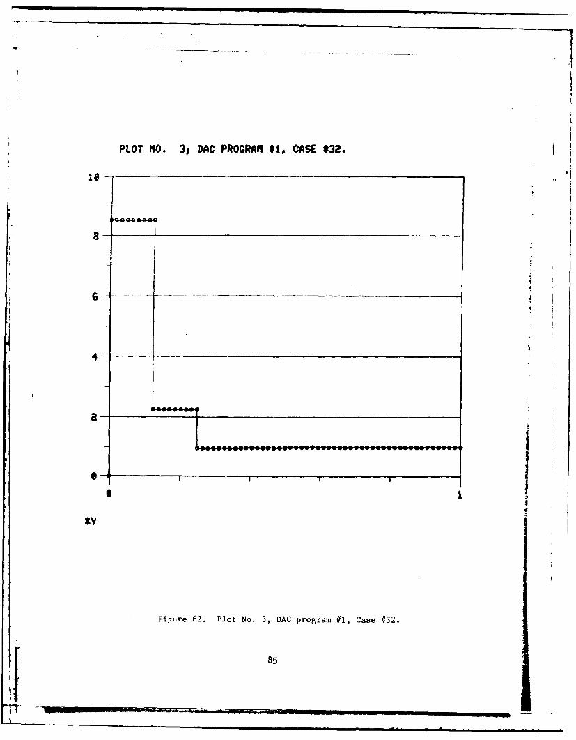
similar results have been obtained for other cases, such as Case 31 when
compared to Case 32, the result of which is contained in this report also.
IV. CONCLUSIONS
The study described in this document consititutes the first application
and published results of the discrete-time DAC theory to control systems.
This section of the report presents the conclusions of this study and offers
recommendations for further investigations. The present study has shown the
cancellation (absorption) of disturbance effects for the discrete-time DAC
applied to a control system for stabilization.
The digital computer implementation for the design of the DAC's arrived at
for this example problem (using the methods developed in the appendix)
performed, in each case of disturbance, those functions which it was designed
to perform. The effects of the disturbance inputs were cancelled out by that
portion of the controller which was designed specifically to handle a given
waveform mode disturbance. When the impulse train was not of too high a
frequency, the errors enqendered by the disturbance were settled out very well.
A unique digital computer analysis tool (DDACPl--Discrete-Time Disturbance
Accommodating Control Program 1) has been developed for implementing the DAC
control laws, the equations of the plant being controlled, and disturbance
models. Also, a graphical plot program has been developed, whereby graphical
plots of any dependent variable versus time may be obtained. Both of these
programs are highly ineractive with the computer user. Additionally, the
graphical plot program may be of benefit in obtaining plots of output data
from other programs as well as the DAC design program(s).
35t DI-I

TABLE 6. SUMMARY OF DAC PROGRAM IMPLEME':IATTON EXECUTION RESULTSOBTAINED IN THIS REPORT
ASSOCIATED FIGURES
CASE XT AT OUTPUTNO. T = 0 CWT AWT LISTING GRAPHICAL PLOTS
1 1.0 1.0 0.0 5 6 Through 17
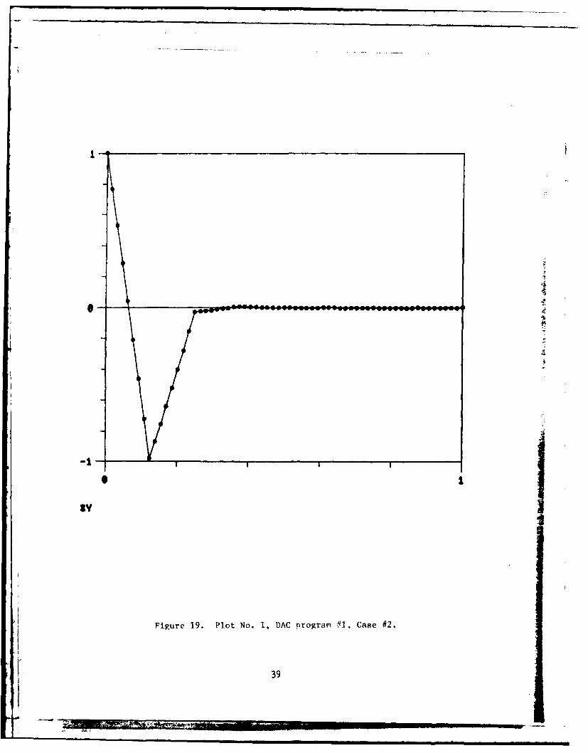
2 1.0 1.0 1.0 18 19 Through 21
3 1.0 1.0 3.0 22 23 Through 25
4 1.0 1.0 10.0 26 27 Through 29
101 1.0 1.0 0.0 30 31 Through 33
202 1.0 - - 34 35 Through 45
29 0.0 1.0 0.0 46 47 Through 48
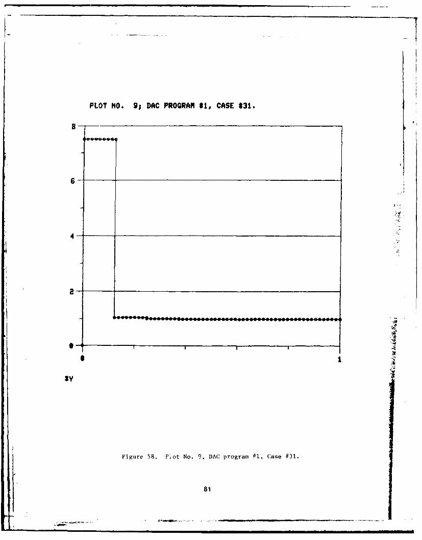
31 1.0 1.0 0.0 49 50 Through 59
323 -1.0 -1.0 0.0 60 61 Through 64
46 -1.0 -1.0 0.0 65 66 Through 69
1WT includes a random noise between +1 input with a random number generatorsubroutine.
2ThThe constant piecewise disturbance was programmed within the main discrete-time DAC program as a function of time by the usage of the FORTRAN IFstatement.
3The program contains the statement: IF (T . LT. ST) UNT = UP.This statement prevents the "overshoot" in the plant (system) outputvariable X, and hence, Y.
36
r *---

It is suggested that future study and investigation be directed to the
following areas:
1. The non-zero set-point regulator control problem.
2. The servo-tracking control problem.3. The design of a discrete-time DAC for a general second-order plant o
(system) with a first-order disturbance.
4. The applications of discrete-time DAC to a discrete control problem.
(This would be beneficial in view of the trend toward using sampled-data and
microprocessor techniques in future designs.) These may include pointing and
tracking of designators, gun pointing, autopilot disturbance compensation
and guidance algorithm design.
3
I
" 37
... 1 -

1a, PROGRAM .I., CASF #2INF'II XT - I.0FOR FXPONENTIAL rtfSTURPANt;F(S):TNPIJT CWT = 1.0THFIJT AWT .I.0
DAC PROGRAM FXAMPI F' NUMFFR I.OUTPUT FORMAT'
TIME XDT YT YT YNTlIp Uri INT T M P:IXTNPT XINT 7HNT K WT
O.O0000E+00 -0.15021E+02 0. O000E+0.1 O.10000E+01-0.85104E+0i -0.85104E+01 -0. 17021E+0? -0.80000E+010.90652E+01 0.00000E+O0 0.80000E+01 -0.85104E+01 0.10000E+01
0. i0000E+0I -0.15099F+00 0.37293F-07 0.37253E-07-0.31 ,. 704F-06 -0.28693E+01 --0.28693E+01 -0. 29802E-060.30563E+01 0.26972F-fO4 0.'..,6972F+01 -0.85104E+01 0.27183E+01
CASE PARAMFTERS"INTEGRATION SCHEME: RIJNrA.-KJTTA 4TH ORDERINTEGRATION STEP SIZE: IT - 0.1,625E-01SAMPLE INTERVAI.: ST = 0. 12500E+00DISTURBANCE: WT - 0.27183E+0:l.FOUATION FOR UNT: UNT = UP + liDSTEADY STATE OIJTPUT: X(T; - "-0.23,)91E'-02
Figure 18. Output listing (condensed) of results, Case #2.
38
,. . i - - -I -
:3 ill

Figure 20. Plot No. 1, DAC program #1, Case #2.
40

411
*Af

DAC PROGRAM #1, CASE #3INPUT XT = 1.0FOR EXPONENTIAL DISTUROANrE'):INPUT CWT = 1.0INPUT AWT =.0
DAC PROGRAM EXAMPLE NUMFR 1.OUTPUT FORMAT:
TIME XDT XT 'YT YNTliP UP UNT TMPXINPT XINT ZHNT K WT
).O0000E+00 -0. 17438E+02 0. I000E+O1 0. 10000E+01).851LO4E+01 -0.10928E+02 -0.:19438E+02 -0.90416E+01).13155E+02 O.O0000E+00 0.90416E+01 -0.85104E+01 0.IO000E+01
).IOOOOE+Oi -0.36272F+01 -0.22352E-07 -0.22352E-07
).19022E-06 -0.23713E+02 -0.23713E+02 0.20210E-06).28547E+02 0.19620E+02 0. 19620E+02 -0.85104E+01 O.20086E+02
CASE PARAMETERS:INTEGRATION SCHEME: RI.JNGA-KUTTA 4TH ORDERINTEGRATION STEP SIZE: PT = 0.15625E-01SAMPLE INTERVAL: .ST = 0.12500E+00DISTURBANCE: WT = 0.20086E+02EQUATION FOR UNT: UNT = UP + UDSTEADY STATE OUTPUT: X(T) -0.56675E-01
4
Figure 22. Outnut listing (condensed) of results, Case #3.
42
......-...-- .,,., - . - " -- .

if
1-
I-
0-
4'A--
-1
-B- I I
S I
Figure 23. Plot No. 1, DAC program ~!l, Case #3.
43
K -- - -. ,

-S -
Figure 24. Plot No. 10, DAC program #1, Case #3.
44

-~ II
ii25-
as- I15- 1
Ia
I I
S I
gy
Figure 25. Plot No. 11, DAC program #1, Case ~3.
345

rt(AC PROGRAM #1.7 CASE t4
INPUT XT = 1 .0FOR EXPONENTIA DTST1.JRTANCE0).-INPUT CWT - 1.0INPUT AWT - 10.0
1 A1C PROGRAM EXAMPLE N.MPFF, J1.O!TPUT FORMAT:
TTMF XDT XT YT YNTt IP t ID UNT TMPIXINPT XINT 7HNT K WT
0.0000F+0 -0.,32724F+02 0.1000-0F+01 .10000E+01-0. R510.4E+01 -0* ?.42614F+0? -0. 34724F+02 -0. 13326E+020.46514E+02 O.O0000E+00 0.13326E+02 -0.85104E+01 0.tO000E+01
0.10000E+Oi -0.18016F+05 0. 38147E-04 0.38147E-04-0.32465E-03 -0.40043E+05 -0.40043E+05 -0.50836E-030.71051E+05 0.20357E+05 0.20357E+05 -0.85104E+01 0.22026F+05
CASE PARAMETERS:INTEGRATION SCHEME: RINGA-KUTTA 4TH ORDERINTEGRATION STEP SIZE: DoT = 0.15625E-01SAMPLE INTERVAL: ST " 0.1.2500F+00DISTURBANCE:. WT = 0.22026E+05EOUATION FOR UNT: UNT - UP + UDSTEADY STATE OUTPUT: X(T) - -0.28150E+03
,.
Figure 26. output listing (condensed) of results f'or Case #4.
46
.. .

-5 71-1
Fiyure 27. Plot No. 1., DAC nrogram #1, Case #4.
47

X19 4
1-
S I
Vigure 28. Plot No. 10, DAC programn Pl, Case #14.
48B

lose@ -
eese-
494

00 0 0 00 * 00+4 I+ + +4+ *+
waUSw w WW W usWcu 41 0r- CU r- OW W nP340 0 UPi' M 3 * 0 co 00
Cb 00P mb me me @2W
000 a@ 00 00 0 a0@+ + + +
w W jiaL www &Jww kWW WWW wM
#.-a *qq Moo wooW ove- vwa Vma 00@V0 @00w0Wq0V-000 tocI- w MO MOW. 0.4. u1). 4w in f'-0. W W tl
00-b 1,--0 e o "W o wow wW 00 I.4-6 4; 606 4; ; 44 4'300 a
I I I I I I I I
.4U. 0014 o.4.4 *.0 .4wo' iofte00 000 @00 000 MOM
W~lww wwpw aww w
UD M u 0.d 0IV4 wUP v .4 W ,, Wm
(*30 *D 4.4C a~4 o 3a at aD 9-. abr u4.4~1 IS w4 v. w w4 ar NO *aa a
wA @00 000 4 @4 ;4d 00 00 00. i
W -000 000 a0 a MoowOib3 4A3 w 4 + T + 44++4 +4 4+ + 4a "4 si w wWW WW WW w W Id WW Wu c I. 1- '04q Ir g we r4- v r'- v 9-01- v
E 11- Z Cu @ 604 ('.4 P-4. w mo v96 Joe C Q n" v 4a o W44 : Mo.* 6 .4 OnoI 40
.o4zC 4 . Xa 2ZX 'MM Mo@ Pv-O U@ w ow 000 M' 0)
.43 I. s .- a W4 9% a w P. 00 a a *a
C U e I .5 S I
0.S-W3- =. 0.44 ~ Mae. 0..4 0M= I0MO00 e a 000 0 0 00 0
C>4LCrILCL 0 1- 4+4+ 5+4 +4 + 444+ + + +czOzx C~ = I- wWW WWW WW LiW WW iWWW Iii
1& 0-4- Q. .w & a.4 .4o w m o o - 0 - e v o' a
U *o3 060- 4-4 .4 r.4 Mr- '
50
e0 ee ee ee1 M e +0 *@ 0 e *e+.4 +. I .4 T. T.4 T.4 +. T + + +4 +4+
Wgo usf' W W WW WW M W 'MWl 'W0 V C% WW r c) 4 %.. 00M e We Vw 06.. mW* WU) V W M')4D * r- f- M V4fl *a b ft 0ob mr- ab meb em ow 0a me m- Eo0 bW r- 040 2 a a. We 0~ 0 0 w -
40 ob *n V . *0 C W4 V W4 so 4 ..
ccp *@0- ** @0 0o. 6- 0 C** e03 c ew W* ** we we00 MO Ma MO mo Mo Mo o o o
++ 1 + 1+ 1+ 1++ 11+ 1+ 1+ 1 1+
CV) C! '~ w" w 11 G C ! U, 0 'Aewe V W0 eW eW ew C.U -
~~00 eee eemeoe ceeco Moe W+ + I IIT T + +S 0+ I + IS ++ I I ++
WMW WWW WWW W WW W WW W WW WWW WWW WNW WW.. W V.44 3V .Mai webi W4W 4D woe W4 'r s r-m eft aes Wm s qh' .1 W MMs V M W4 wq 91 Ie's M's e'w Maoe Mao MeM Mw -Ocw Ww MaeC
mewwe 'se WMWu 'sWW eva ewm r-o 0 e W W InIVIWCu ra_ mom Ma44.~ 0 we wine mine W-a IS-e 0 i i-
+4 .. . . ... ... .4. + .. 4 4.4.4 4.4.4 4++ 4.'MW WWW WWW WWW WWW WWW WWW WWW WWW WWWW wt M0U w04 W M rt- W4 *'-wo qW 9- CUW r- isMo -'b M einU
-4.4 V060 a Ve-4 We e a ~ m W O MW WI-M' c- 0' CSS-cc 00eeee woo woo mom rmomwi V w 0 'IV ft5-44 a:4f~ G4!' a.- ao- ae Me= sme mom a e*- a
*1 0 *O Ma *0 Mo . 00 ** C * 4D * 0 MO 00 MOM CCC C -
'MW WAWW WWW WWW WWW W WW WWW W IWW WW'M WWWIVW MC3 0C eq em- es- -e0r-iP- evw e*W ewe eve *.45Ms 4.4 wine eaw 10601 eWNW Oee' *-.r- ao-4- 0 r- M0 1,-- a'I'. Mae ow Wine ewa M40we we V-i efl- ewo-
mm- . V. . u! C 0! *! C! It . .! Ct * 0! * C! * ! * C 0! *iee * ee ee ee ee ee ee ee Mecs0 MMM0DO0M

0 cu
W4 P- Ww a W I4Dl $A a c~4 Uq
a~ .n
WhIW WWW
M ' e. -q0 W U
atw *m
II I
WOO W W 06+4 + + + zWcWWWj WWWj I -@ aen lea Mcn G 3r- qwe W 0
w rw a n 0WU)m *wg*bW - M'~ CD we
*** ** ~U 0W Iq;t Id .401 aC 6- Or
z du~
WawW WWW WMC
***0 IV**% WZUWI--S~~~ M 46 ZCS(.S.
&- c - c&W . us m -
4+, ~ ~ a 6-+ 1)--E b WU& MW WW cE c .P-
+'0 W*-..-ICw U) W U)Wt'- @1063zz "crI0 -.4U *(')@ - Q" U~*LW r- ('Owe
*- W 90 0 .n 9
52

--- 'VOW
Figure 31. Plot No. 1, DAC program' #1, Case #10.
53

544
-1@ -_ ___ ___ __ ___ ___ ___ ___ __ ___ ___ __7 7_

Figure 33. Plot No. 11, DAC program #1l, Case #10.
55

RLIN ,DACF2
AoC PROGRAM fI, CSF f2,INTPU T 1'F - I .0
D.AfC FOGRAM -XAMFI F. i'M IMBFF: IOUTFIJT FORMAT:
TTME XDT XT -T YNTUP UP I INT TP
TI NT 7HNT I
0..0@000E+O00 -0.1402IF-O2 0. •i OFfOl 00.0.I000EO.-0.85.10 IF+O1 -'0. 7,'.! 04+IO 1 -0. 16021E4-02 -.-0.751O4E+010.7,5104E+Oi 0.00000F+O0 0.75I04E+0:I -.0.85L04E+O] 0.10000F+01
0.6250OF--0:[ -0.14918F+0? 0.J0294E+O0 1, OOOOE+01-C.95104E-f0.I -0.75104E+01 -0..160?lE+02 0.75104E+010.7-:10IF+O1 0.O0000E.fO O.75104F+01 -0.85:104E+01 O.10000E+01
O. 12500E+00 0.62799E+01 -0.85150F-00 --0.85150E-OOO.72467E.-01 -0.111.53E+01 0.6:13L4E+01 0.63951E+010.11153E+01 0.75104E+01 0. 11153E+01 -0.85104E+0I 0.O10000E+01
0.18750E+00 0.66817F+01 -0.44972E+00 -0.85150E+000.72467E+01 -0.1I1153E+01 0.61314E+01 0.63951E+010.11153E+01 0.75104Ef0i 0.1.153E+01 ---0.951.04E+01. O.:LOOOOE+OI
0.25000E.-OO 0.21853E.-0O -O .2222.E-01 --0.22222E-O10. 18912E+00 -0.94837E+00 .-0.75925E.+00 0.16690E+000.94837E+00 0. 11153E01 0.94837E+00 -0.851.04E+01 0.10000E+01
0.31250E+00 -0.57675E+01 .-0.8240SE-02 -0.22222E-01.0. 18912E+00 .-0.94837E+00 -0.75925E+00 0.16690E+000.94837E+00 0.11153E+01 0.94837E+00 --0.85104E+01 -0.50000E+01
O.37500E+00 -0.28182E+00 -0.37725E+00 -0.37725E+000.32105E+01 0.18849E+01 0.50954E+01 0.28333E+01
-0.18819E+01 0.94837E+00 -0. 18849E+01 -0.85104E+01 -0.50000E+01
0. 43750E+00 -0.29986E+00 -0.39528E+00 -0. 37725E+000.32105E+01 0.18849E+01 0.50954E+01 0.28333E+01
-0.18849E+01 0.91837E+00 -0.18849E+01 0.85104E+01 -0.50000E+01
0.50000E+O0 0.31105E+01 -0.4.1146E+00 -0.41446E+000.35272E+01 0.49977E+01 0.135249E+01 0.31128E+01
-0.49977E+01 -0.18849E+01 -0.49977E+01 -0.85104E+01 -0.50000F+0I
0.56250E+00 0.33095E+01 .-0.21545E+00 -0.41446E+000.35272E+01 0.4997 7E+01 0.85249F01 0.31128E+01
-0.49977E+01 -0.18849E+01 -0.49977F+01 -0.85104E+01 -0. 50000E+01
0.62500E+00 0.53461E-01 -0.37133F--02 -0.37133E-020.31602F-01 0.9025AF+01 0.50572E401 0.27889E-01
-0.50256F+01 -0.49977E+0i -. )2 -0.85.104E+01 -0.000ffO
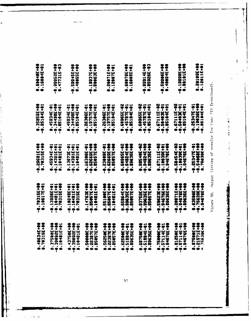
Figure 34. Output listing of results for Case #20.
56

O.687OF4O0 0,569RIF-01 -O..'Y289F-03 -0.37133E-020.31602E-01 0.50256E+01 0.272r+Oi 0 ?7889F-01-0.50256F+O -0.49977F+Oi -.0.50256F+01 ..-O.0 5104EOl -0o.50000E+01
0.75000E+00 0.13995F+01 0.24140FfO0 0.24140E+00-0.20544F+01 032125E+01 O. l158t F+01 -0.19130E+01-0.32.i25E+01 -0.50256F+o1 .-0 .31?5F+01 -0.85104F+01. O.OOOOOE+0'
0.31250EfOO 0.14890F+01 0.3309FO0 0.24140E+00-. 2..44E+O1 0.32125FfOl N. tRs I t+01 -0.18130E+01-0.32125F+01 -0.50256F+0:I -.. 32125F+01 -0.85104E+01 O.OOOOOE+O0
0.87500E00 -0.31895E401 0.42621EfO0 0 .42621E+00-0.36272E+01 O.1J906F.-01 "-0.36157E+01 -0.32010E+01-0.11506E-01 -0.32125E+01 "-0.11506E-01 -0o.85104E+01 O.OOOOOE0'
0.93750E+00 -0.33936F+01 0,22:15F+00 0.42621E+00-0.36272E+01 0.11506F--O1 0.36157E+01 -0.32010E+01-0.11506E-01 -O.32125F+01 -0.11506E-01 -0.85104E+01 O.OOOOOE+O0
0.10000E+01 0.99361E+01 0.50234E-02 0.50234E'-02-0.42751E-01 .-0.26222E-01 --0.68973E-01 -0.37728E--010.26222E-01 -01i506E-01 0.26222E-01 -0.85104E+01 0.10000E+02
0.10625E+01 0.10572E+02 0.64073F+OO 0.50234E-02-0.42751E-01 -0.26222F.-01 -0.68973E-01 -0.37728E-010.26222E-01 -0.11506E-01 0.26222E-01 -0.85104E+01 0.10000E+02
0.11250E+01 -0.17463E+02 0.11609E+01 0.11609E+01-0.98795Ef01 -0.87448E+1O -0.18624E+02 -0.87196E+010.87448E+01 0.26222E-01 0.87448E+01 --0.85104E+01 O.OOOOOE+00
0.118?5E+01 -0.18581E+02 0.43555F-01 0.11609E+01-0.98795E+01 -0.87448E+01 -0.,9624E+02 -0-87186E+010,87448E+01 0.26222E-01 0.87448E+01 -0.85104E+01 O0.OOOOOE+00
0.12500E+01 0.84577E+01 -0.11452E+01 -0.11452E+010.97465E+01 -0.14357E+00 0.96029E+01. 0.86012E+010.14357E+00 0.87448E+01 0.14357E+00 -0.95104E+01 O.OOOOOE+00
0.13125E+01 0.89988E+01 -0.60412E+00 -0.11452E+01
0.97465E+01 -0.14357E+00 0.96029E+01 0.86012E+010.14357E+00 0.87448E+01 0.14357E+00 -0.85104E+01 O.OOOOOE+00
0.13750E+01 0.28264E+00 -0.28374E-01 -0.28374E-010.24148E00 0.69533E-01 0.31101F+00 0.21310E+00-0.69533E-01 0.14357E+00 -0.69533E-01 -0.85104E+01 0.OOOOOE+00
0.14375E+01 0.30072F+00 -0.:10291E-01 -0.28374E-010.24148E+00 0.69533E-01 0.31101E+00 0.21310E+00-0.69533E-01 0.14357E+00 -0.69533E-01 '-0.85104E+01 O.OOOOOE+00
0.15000E+01 -0.64885E-01 0.89488E-02 0.89488E-02-0.71t58F-01 0.23236F.-02 -0.73834F.-0i -0.67209E--01-0.23236E.-02 -0.69533F-01 -0.272:16E-02 -0.85104E+01 O.OOOOOF+00
Ptiure 34. Output ]Hstiny of results for Case #20 (continued).
57
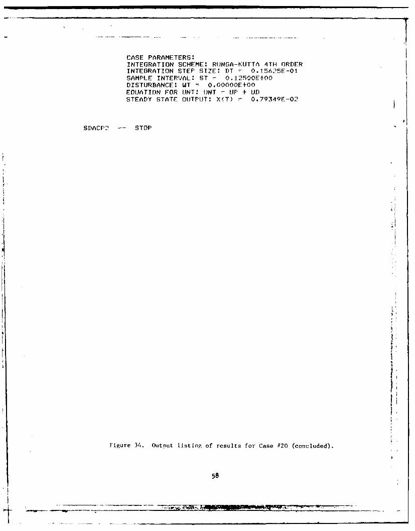
CASE PARAMETERS:INTEGRATION SCHEME: RUNGA-KLJTTA 4TH ORDERINTEGRATION STEP SIZE: iT - 0.15625E.-O.SAMPLE INTERVJAL ST - ,. 1 2500E+O0DISTURBANCE: WT O.OOOOOE.0EQUATION FOR I.JNT* UINT - IP + USTEADY STATE OUTPUT: X(T) 0.79349F.-02
5
SDACF2 -- STOP
I
Figure 34. Output listing of results for Case #20 (concluded).
58
.I I.. = , - -

-- 4
Figure 35. Plot No. 1, DAC propran #1, Case #20.
59

2-.
Figure 36. Plot No.-1 DAC programi #1, Case #20.
60

Ll.
Fig~ure 37. Plot No. 3, DAC program #1, Case #20.
61

Mum-
Figue 3. Plt N. 4 DACproram#1, ase#20
5-2
-5 - - __ ____ ____ ____ ____ __7,
AA

-1.- _ i I I I I
f
Figure 39. plot No. 5, DAC progran 01, Case #20.
63
Il pa a l 1111 • .

10
6 I I
1a
Fiure 40. Plot No. 6, IAC nropram #'l, Case #20.
64
t _ _ _ _ _ _ _
in-i i i l V

PLOT NO. 7; DAC PROGRAM *to CASE $20.
e-
I
II
-s - ,- .
S 1 2
Fiure 41. Plot No. 7, DAC program 1 Case #20.
65

I I I I I
T7
10-
0-
-5 - _______________
Figure 43. PloL No. 9, DAC program /1, Case #20.
66

20
Is-V
I I I ILane II
Figure 44. Plot No. 10, 1)AC program #1, Case #20.
67
PT__ __

PLOT NO. llj DAC PROGRAM #l, CASE $20.
Figure 45. Plot No. 11, DAC program #1, Case #120.
68

DAC PROGRAM #I, CASE #29INPUT XT 0.0FOR EXPONFNTIAL bITSTJRRAMCFS SINPUT CWT 1.0INPUT AWT 0.0
DAC PROGRAM EXAMFLE NUMFER 1.OUTPUT FORMAT:
TTMF XrT XT YT YNT(IF UP[ JNT TMPIXINPT XINT ZHNT K WT
C'. 0000F+00 0. IOOOOF+01 O.00000E+O0 0,00000E00O.0)OOOF+00 (.O0000OE+00 0.O0000F+O0 .OOOOOE+O00.000OOE+O0 O.OOOOOF+00 0.OOOOOE+00 -0.85104E+01 0.10000E+01
0.10OOoE+01 O.11921E-06 -0.139,0E-O, -0.13970E-070. 1RR, F-06 -0.10000E+01 0.10492E-060.10O,,OE+o0 0.0 +1 0.10000+ol -0.85104E+01 0.10000E+01
CASE PARAMETERS:INTEGRATION SCHEME: RUNGA-KUTTA 4TH ORDERINTEGRATION STEP SIZF: DT - 0.15625E-0SAMPLE INTERVAl.: ST - 0.12500E+00DISTURPANCE: WT = 0.10000E+01EQUATION FOR UNT: UNT UP + LiDSTEADY STATE OUTPUT: X(T) -0.12107E-07
TTO -- STOP
Figure 46. Outnut listing (condensed) of results for Case #29.
69
I .. .- .. ... .. '. .. . ... '. ..

PLOT NO0. 11 DAC PROGRAM $1. CASE $29.
6.2y
Figue 4. Plt N. 1 DACproram#1, ase#29
6.70
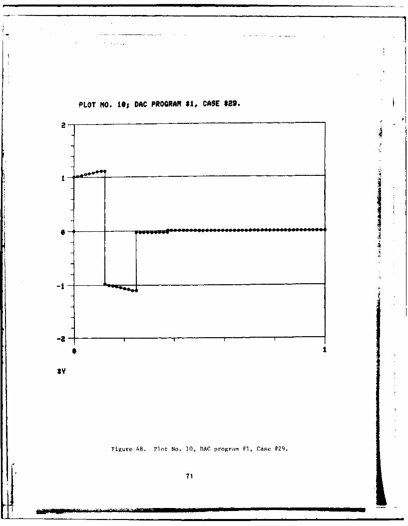
PLOT NO. 10; DAC PROGRAM 81, CASE $29.
4- 0
1-1
...-......

DAC PROGRAM ti, CASE 31INFUT XT - 1.0FOR EXPONENTIA DISTURBANCE(S):INPUT CWT 1.0INPUT AWT 0.0
DAC PROGRAM EXAMPLE NUMBER 1.OUTPUT FORMAT:
TIME XDT XT YT YNTtiF Uri UNT TMP1XINPT XINT ZHNT K WT
O.OOOOOE+00 -0.65101E+01 O.1000E+01 0.10000E+01-0.85104E+0:[ -0.75104E+01 -0.85104E+01 -0.75104E+01O.O0000E+00 O.O0000E+00 0.75104E+01 -0.85104E+01 O.1000E+01
0. IOO0OE+O 1 0.0000E+00 0.93132E-09 0.93132E-09-0.79259E-08 -0. I0000E+01 -0. 10000E+01 -0.69946E-08OI.OOOOE+01 O.10000E+01 0.10000E+01 -0.85104E+01 0.10000E+01
CASE PARAMETERS:INTEGRATION SCHEME: RUNGA-KUTTA 4TH ORDERINTEGRATION STEP SIZE. DT .015625E-01SAMPLE INTERVAL: ST = 0.12500E+00DISTURBANCE: WT = 0.10000E+01EQUATION FOR UNT: UNT = UP + UISTEADY STATE OUTPUT: X(T) 0.93132E-09
Figure 49. Output listing (condensed) of results for Case #31.
72

PLOT NO. 1; DAC PROGRAM #1, CASE 831.
taj
Figure 50. Plo. No. 1, flAG program #1t, Case #31.
73

PLOT NO. 2j DAC PROGRAM #1, CASE $31.
- S 1
sy
Figure 51. Plot No. 2, DAC program #1, Case #31.
74
- I

PLOT NO. 31 DAC PROGRAM #I, CASE $31.
-2 -
4
-8
*1'-l1 -- I I
S
gy
Figure 52. Plot No. 3, DAC program #1, Case #31.
75

PLOT NO. 43 DAC PROGRAM S1. CASE $31.
-2 -
-6 -
Figure 53. Plot No. 4, DAC program #1, Case /31.
76

PLOT NO. 53 DAC PROGRAM $1, CASE *31.
2--
-e -
-4
-6 -
-8 - _ _ _ _ _ _ _ _ _ _ _ _ _ _ _ _ _ _ _ _ _ _ _ _ _ _ _ _ _
S Y
lv &
I
Figure 54. Plot No. 5, DAC program #1, Case #31.
771

PLOT NO. 63 DAC PROGRAM 81, CASE 831.
2
- g ---- ----- -- -- --
Figtirc 55. Plot No. 6, DAC program 11 * Case #31.
78
~~Aw,

PLOT NO. 7; DAC PROGRAM #I, CASE *31.
2 -
Figure 56. 1,Lot No. 7, DAC program #11, Case #'31.
79

PLOT NO. 8; DAC PROGRAM #I, CASE 131.
-44
--
S I
80
PLOT NO. 9j DAC PROGRAM $1, CASE #31.
4-2-
II
ly
Figure 58. Plot No. 9. DAC program #1, Case #131.
81F-gure 58.-P.ot-No.-9--.---program --l-.Case-/- -

PLOT NO. 10j DAC PROGRAM #1. CASE #31.
-2
-4
-6
-8-
o1
*Y
Figure 59. Plot No. 10, DAC program 1, Case #31.
82

+ + 4
V- IV 0 W
z Ic 0 4 -4 -aW
r:0 C 0!
94949 ~ 09
000 @00
= 40 000nW + 0
w0 *00 000 b~u4* C
hihi I--:Q- CLi vve 0 IL
0A it ss** 00:094c min W4 @0
ic x@ I 00 000 w w-*
m m i aa- LL
CL ~ ~ 9494 09494 I 549j1-4
hP4 I-
P. .- q ~ -n M Ch
ILI00c0 hhh 6u6
CV) hiii hhh 2£46
~ 00 i A. *tO O)0 m494A~83

PLOT NO. 1; DAC PROGRAM #I, CASE $32.
1-
0SrY
L.1
Figure 61. Ilot No. I DAC program I Case #32.
84
PLOT NO. 3; DAC PROGRAM $1, CASE $32.
e --
8-
6-a
4-
2-
0I
FIt~ure 62. Plot No. 3, DAC program Ill, Case #32.
• 85

PLOT NO. 103 DAC PROGRAM S1, CASE #32.
B-
6--S_ _ _ _ _ __ _ _ _ _ _ _ _ __ _ _ _ _ _ _ _
4- ur 63-ltN.1,PCpo-rm#,Cs-#2
4 ______86

PLOT NO. 11; DAC PROGRAM #I, CASE $32.
4 4
0
SN\N\Y
Figure 64. Plot No. 11, DAC orogram ff1, Case #32.
87
I-I Il I I I in-..

Ttf)C FROGRAM t1, CAcSE #46INPUT XT - -1.0FOR FXF'ONFN'rTIL DT,- 1IJRr4A NCF (S)
NPIFIT CWT 1.0INFlI oWT 0.0
DAC FFOGRAM EXAMFI.F NUMEFR I.ouT-Ur FOBFAT:
I: TIT x r Yr YNT
1F U.Pt UNT TMP 1
X TINFT XTNT ZHNT K WT
O.O0(OOF+00 0. 1.021F+02 -0. 1O0000+0I -0. 10000E+01
0.pS[0 1+ k)I 0.75,.04F.I o.16027F+02 0.75104F+010 ,745 10 .E'+501 -o.5104E+01 -0.10000E+01-0 .7 "': 1 , 4 F". () I 0.O00001"if.-I00 '0 7 1 h 'O 0° 1 4 40 0•I 0 0 +
--14918F+02 .-0 10294F+00 ..-0o.:LOOOOE+01
0.SUc'1FOI 0.75]. Of1F01 0 . :[ 602.I. E+02 0.75104E+01
-O 0.7 IE 1. 0.O00000F+00 .- 0. 751 04F10 .- 08 O104E+O: --0 000E+0
-'-,.".. 0 -0. 62799F7-+,(),[ 0.85150F+00 o.851,50E4"00-2 ' °4 7F I(" Cl. 1:1.J. '+0o -0 6131 IE+01 "-0 ,63951E+01
0.). 12001.10000E99+:1 0 3+010+0 .8i0F0-0- I I ff3 40I1 -0. 75104E'1. -0. [ 1:153F+0.[ .-0.85104E+01 -0.lO000E+OI
U. IR, 750)+0 -0,668:E+01 0. 44972EJ00 0.85150E+00
0 724'. -01 0.I1153E+01 - 0. 61314E+0I -- 0.6c395;LE+Oi O O E
- .i j 3Ff.t -0.751041F..0.1 -0.111.53r +01 .-085104E-+01 -0.IOOOOE+0i
". "F -0 . 0. 22222F-01 0..22222E-01
-0. ?I i2E 00 0.94837F-4-00 0.75925E+00 -0.16690E+00
-0.94837E+00 .,11153E+01 -0.94837E+00 --0,B5104E+01 -0.1OOOOE+01
0.31250F+00 -0,23251E+00 0.82408E-02 0.22222E-01
-0. 18912E+00 0.94S37Ef00 O.75925E+00 -0.16690E+00
-0.94837F+00 -0. 11153E+01 -0.94837EfO0 .- 0. 85104E+0:L -0.1O000E+01
0 * 37500F+00 0. 480,6F-01 -0. 66351E-02 -0. 66351E-02 4O. 56467F-01 0,99820E-100 0.10547E+01 0.49832E-01
-0.99820F.-0 --0.94837E+00 -0.99820E+00 -0.85104E+01 -0.10000E+0I
0.43750F 00 0,5 109E-0:1 -0.35618E-02 -0.66351E--02
0.56467E-01 O.c ?820E+00 0.1I0547E+01 0.49832E-01 3
-0.99820F1-00 -0.94837Ef00 -0.99820E+00 -0.85104E+01 -0.IO000E+01
0,5000OFf 00 0.25864E-02 -0.29179E-03 -0.29179E-03
0.24832E-02 0.10004E+01 0.10029E+01 O.21914E-02
-0.lO004EFOt -0.99820E+00 -0.10004E+01 -0.B5104E+01 -0.10000E+01
C,.56250F+00 0.27518E-02 .-0.12631E-03 -0.29179E-03
0.24832E 02 0.10004E+01 0.10029E+01 0.21914E-02
-0.1004E+-I. -0.99820E+00 .-0.10004E+01 -0.85104E+01 -0. I000E+Oi
Figure 65. Output lsting, of results for Case #46.
(88

w LL. LLaj wa LL a,o 0 0 0 0 C' 01
o o 0 0 0 0 0
oO 00 00 00 00 00 0
o1 0 c l 00 r o 0 o 0 M 0 0 nC 0M) " ~ r, M 0 00 4 0t -4 Cl - -
o; 0000 00 00 00 00 0I I I
u-v
coo 000 000 000 000 000 000 r n1-4 ++ ++ I I-I 11-4 ++4 I ++4 I + : r 4
L. WUl wwLw LaL W W I4LLI LJ WJHJ WLAJ w Cw i 00
m' o o ri3 00-N4 010 v 0 0N' OM,-0 W- -v n
tr le .0 o0-II To 4 0 oo o 4+ mQ
ol0.0 00 01 i00 V,000 0 00 000 In000 , )04
1 o Lr
000 000 000 000 000 000 000 N Z.I 4 + 4 1++ 1I-.. 1+ I--4 1++4 1+-t - I= - C
LJ W LAI ~ a LawL.J wWJ WWi. w~I wWj I-w w w wwJww )t0O V m0 0 'I"-0 040 00 4w0 0 m00 10 0 P C
r4 o o 1-o reo -' 000 0-00 1 0 0 N0 0 wx -j - zh)0- '0 cJoo0 ~O 0 tmoo U 000 In 0 0 a I-0C3 = 0
tQ- q-- r4 -' 4 0--V4 4 M' V4 4 4 4 m w- 00 En S.~~ ~ . .. . I- X . -
000 000 000 000 000 000 000 Ii C'w LI I I I I I I f 0 0 1- 0Cw <
IL .X WX >-M'' r)40 pn O,-4 174 0f~. '0 - (D II -1P--
000 000 000 000 000 000 000 N OZ'.-<+ + +I+ +1+ +4 I4 1+ +4 1+ + w .- - = CUai W U WJ W L.IWW wwawa L w w W LJ wW IjW0 ui CZZC -
ov ovo 0~00 000 ov10 ovo MOO in.C~ir- M0 N000 e-OM0 NOVC0 I -O 0 MO O 00 j0.~ I-Iri r4o 1170 ri6 ; 00 '00N0 NWOO o 000 OWI IlZ
N'4 M43 ,4 r',4 ri c ri4 m F4 -4 (j.4.4 m. -4 W
000 000 000D 000 000 000 000 WZWII I I I I II I EC I-L2 aC
89,ZZ l
~~A O

PLOT NO. 11 D C PROGRAM 1,, CASE $46.
gy
Figure 66. Plot No. 1, I)AC nrogran 111, Case #46.
90
...- rr... I I - - -
-I - w ---II I I

PLOT MO. 3; DAC PROGRAM 01, CASE $46.
20-
-t
sy
Figure 67. Plot No. 3, DAC program #1, Case #/46,
91

PLOT NO, 10j DAC PROGRAM S1, CASE $46.
292
5-
-10 - "r
SY
F i ,'ire I, ' Ilot No. I (), DA(C program J Il, Carse hA 6.
92

AfD-A105 802 ARMY MISSILE COMMAND REDSTONE ARSENAL AL GUIDANCE A--ETC F/6 19/2(UDIGITAL COM4PUTER IMWtEMENTATION OF A DISCjRETE-TIME DISTURBANCE ---ETC (U)
UNCLASSIFIED DRSMI/RG-ao-27-TR SGIE-AO-E950 15a NIL

PLOT NO. 11; DAC PROGRAM $1, CASE 146.
WNN

BIBLIOGRAPHY
1. RSX-11D User's Guide, DEC Order No. DEC-11-OSDDUA-A-D, DigitalEquipment Corporation, Maynard, Massachusetts.
2. RSX-11D Task Builder Reference Manual, DEC Order No. DEC-11-OXDLA-C-D,Digital Equipment Corporation, Maynard, Massachusetts.
3. PDP-11 Fortran Language Reference Manual, DEC Order No.DEC-11-LFLRA-B-D, Digital Equipment Corporation, Maynard, Massachusetts.
4. PLDT/1D Terminal Control System 40DZA User's Manual, Tektronix, Inc.,Document No. 062-1464-00.
5. PLDT/ID Advanced Graphing II User's Manual, Tektronix, Inc.,Document No. 062-1530-00.
6. PDP-11 Fortran User's Guide, DEC Order No. DEC-11-LFPUA-B-D, DigitalEquipment Corporation, Maynard, Massachusetts.
REFERENCES
1. Johnson, C.D., "Disturbance-Accommodating Control Theory for Discrete-Time Dynamical Systems," Final Report on Contract No. DAAK40-79-M-O028,July 1979.
2. Kelly, W.C., "Theory of Disturbance-Utilizing Control with Applicationto Missile Intercept Problems," Technical Report RG-80-11, US ArmyMissile Command, 12 December 1979.
3. Malcolm, W.W., Priest, J.H., and MoTigue, L.D., "The Development of aDisturbance-Accommodating Controller to Reduce 'Spot Jitter' in aPrecision Pointing System - A Practical Design Guide," TechnicalReport TG-77-21, US Army Missile Research and Development Command,1 July 1977.
9"

DISTRIBUTION
SNo. ofCopies
Defense Documentation CenterCameron Station 12Alexandria, VA 22314
US Army Materiel Systems Analysis ActivityATTN: DRXSY-MP 1Aberdeen Proving Ground, Maryland 21005
ITT Research InstituteATTN: GACIAC 110 West 35th StreetChicago, Illinois 60616
CommanderUS Army Research OfficeATTN: DRXRO-PH, Dr. R. Lontz 5P.O. Box 12211Research Triangle Park, North Carolina 27709
US Army Research & Standardization Group (Europe)ATTN: DRXSN-E-RX, Dr. Alfred K. Medoluha IBox 65FPO New York 90510
CommanderUS Army Material Development & Readiness CommandATTN: Dr. James Bender I
Dr. Gordon Bushy 15001 Eisenhower AvenueAlexandria, Virginia 22333
HQ, Department of the ArmyOffice of SCS for Research, Development & AcquisitionATTN: DAPA-ARZ 1Room 3A474, The PentagonWashington, DC 20301
OUSDR&EATTN: Mr. Leonard R. Weisberg 1Room 3D1079, The PentagonWashington, DC 20301
DirectorDefense Advanced Research Projects Agency1400 Wilson Boulevard 1Arlington, Virginia 22209
95
.. ,- ,~ ." ' .. . .

DISTRIBUTION (Cont' d)
No. of
Copies
OUSDR&EATTN: Dr. G. Gamota 15Deputy Assistant for Research (Research in Advanced
Technology)Room 381057, The PentagonWashington, DC 20301
Dr. C. D. Johnson1
4001 Granada DriveHuntsville, Alabama 35802
DRSKI-LP, Mr. Voigt1-R. Dr. MeCorkie1-R, Dr. Rhodes1-E1-RR, Dr. Hartman1-RPT (Record Set)1-RG1-RGN, J.A. McLean1
W. L. McCowan1Dr. W. C. Kelly1C. Will1
96

'DATE
,ILMED