AD-A259 433JiJiiii111i~jiijI~Ill 11I!I I i II!! --

Defense Nuclear AgencyAlexandria, VA 22310-3398

DNA-TR-90-171

Analysis of Prolate Spheroidal Shell under Undex Load

David S. NokesCharles Stark Draper Laboratory, Inc.555 Technology SquareCambridge, MA 02139 I%

~JAN14

December 1992

Technical Report

CONTRACT No. DNA 001-89-C-0006

Approved for public release;distribution is unlimited.

93-00849

Destroy this report when it is no longer needed. Do notreturn to sender.

PLEASE NOTIFY THE DEFENSE NUCLEAR AGENCY,A'TN: CSTI, 6801 TELEGRAPH ROAD, ALEXANDRIA, VA22310-3398, IF YOUR ADDRESS IS INCORRECT, IF YOUWISH IT DELETED FROM THE DISTRIBUTION LIST, ORIFTHE ADDRESSEE IS NO LONGER EMPLOYED BYYOURORGANIZATION.

o.04

.

DISTRIBUTION LIST UPDATE

This mailer is provided to enable DNA to maintain current distribution lists for reports. (We wouldappreciate your providing the requested information.)

NOTE:0 Add the individual listed to your distribution list Please return the mailing label from

the document so that any additions,El Delete the cited organization/individual. changes, corrections or deletions can

be made easily.

O Change of address.

NAME:

ORGANIZATION:

OLD ADDRESS CURRENT ADDRESS

TELEPHONE NUMBER: ( )Zcr

WI-uJ

cr DNA PUBLICATION NUMBER/TITLE CHANGES/DELETIONS/ADDITIONS, etc.)13 (Attach Sheet if more Space is Required)Z<I

WIrIuJ

I-I

0'

DNA OR OTHER GOVERNMENT CONTRACT NUMBER:

CERTIFICATION OF NEED-TO-KNOW BY GOVERNMENT SPONSOR (if other than DNA):

"SPONSORING ORGANIZATION:

CONTRACTING OFFICER OR REPRESENTATIVE:

SIGNATURE:

DEFENSE NUCLEAR AGENCYATTN: TITL6801 TELEGRAPH ROADALEXANDRIA, VA 22310-3398

DEFENSE NUCLEAR AGENCYATTN: TITL6801 TELEGRAPH ROADALEXANDRIA, VA 22310-3398

REPORT DOCUMENTATION PAGE FOmBA 070oved

PubiMc Wl' burden Wr this m n og n toninto i msti uad to average 1 hour Per resonse. iictuding the ti•s for nerevn mwructiors. eaching esting datia sourcee.gihednO wad Maintakiing the dit nded. and conlating and refhig the colaction of i do eion. Send =ym e regarding thi burden mtimte or any other apa•d tho*

..ladion oi infaiftion, includig sugestions for reduidng th"' -, In. to Washintgon, Headquartrer Sa . Directorme for Itroniation opations and Reports. 1215 JeffronDavis IgNohy. Suite 1204. Arlngton VA 2220-4302. and to the Ofie of Managenarut and Budget. Pap•Iurk Reduction Proac (0704-018). Wmhington. DC 20503.

1. AGENCY USE ONLY (Leaveu bnk) Z REPORT DATE 3. REPORT TYPE AND DATES COVERED

921201 Technical 890301-900831

4. TITLE AND SUBTITLE 5. FUNDING NUMBERSAnalysis of Prolate Spheroidal Shell under Undex Load C -DNA 001-89-C-0006

PE-62715HPR-RSTA-RF

6. AUTHOR(S) WU-DH055790

David S. Nokes

7. PERFORMING ORGANIZATION NAME(S) AND ADDRESS(ES) 8. PERFORMING ORGANIZATION REPORT

Charles Stark Draper Laboratory, Inc. NUMBER

555 Technology SquareCambridge, MA 02139

9. SPONSORINGIMONITORING AGENCY NAME(S) AND ADDRESS(ES) 10. SPONSORING/MONITORINGDefense Nuclear Agency AGENCY REPORT NUMBER6801 Telegraph Road DNA-TR-90-171Alexandria, VA 22310-3398SPSD/Tsai

11. SUPPLEMENTARY NOTES

This work was sponsored by the Defense Nuclear Agency under RDT&E RMC Code B4662DRS RF 00097 SPSD 4300A 25904D.

12a. DISTRIBUTION/AVAILABIUTY STATEMENT 12b. DISTRIBUTION CODEApproved for public release;distribution is unlimited.

13. ABSTRACT (Aximum 200 word)

This effort was an attempt to verify a newly developed closed-formed solution tothe transient response of a submerged prolate spheroidal shell structure due tounderwater explosive shock loading. Numerical solutions were attempted for threetest cases ranging from a sphere to an elongated spheroidal shell approximating theshape of a submarine.

Results for the spherical case were exactly the same as for the previouslyreported theory which is restricted to spheres. The results for the elongatedspheroidal shells were in error, with the magnitude of the errors increasing as theamount of elongation increased. The errors appear to result from truncation of theinfinite series solutions. As a result, useful results could not be obtained usingcurrently reasonable computer resources.

14. SUBJECTTERMS 15. NUMBER OF PAGESSpheroidal Shell Undex Load 54Underwater Shock Shell Theory 16. PRICE CODEFluid-Solid Interaction

17. SECURITY CLASSIFICATION 18. SECURITY CLASSIFICATION OF 19. SECURITY CLASSIFICATION OF 20. UMITATION OFOF REPORT THIS PAGE ABSTRACT ABSTRACT

UNCLASSIFIED UNCLASSIFIED UNCLASSIFIED SAR

NSN 7540-01-28W5500 Standard Form 298 (Rev. 2-39)Precribed by ANSI Sts- 2M3-IS

298-102

UNCLASSIFIED

SECURITY CLASSIFRCATMO OF THIS PAGE

CLASSIFIED BY:

N/A since Unclassified.

DECLASSIFY ON:

N/A since Unclassified.

SECURITY CLASSIFICATION OF THIS PAGE

UNCLASSIFIED

EXECUTIVE SUMMARY

The objective of this effort was to verify a newly developed closed-form solution to the

transient response of a submerged prolate spheroidal shell structure under the loading of an underwater

shock.

The closed-form solution for the response of a spherical shell had been previously developed

(Ref. 1, 2). Numerical results had been generated for a particular test case. These results had been verified

by an underwater shock testing program (Ref. 3).

The current research has attempted to extend these results to the prolate spheroidal shell case.

A prolate spheroidal shell with a major diameter approximately 10 times the minor diameter is a reasonable

approximation to the shape of a modem submarine. A closed-form solution for this case would be useful

to cross check numerical or finite element solutions for the underwater shock response of submarine hulls.

Graduate student research sponsored by the The Charles Stark Draper Laboratory, Inc., herein

after known as Draper, under Independent Research and Development (IR&D) funding had developed the

theoretical basis for the solution to this problem (Ref. 4). The purpose of this effort was to obtain specific

numerical solutions for comparison with other numerical methods or test data.

Numerical solutions were attempted for three test cases. The first case was an almost perfect

sphere. This case produced exactly the same results as previously reported for the sphere, thus providing a

first cross check of the theory.

The second test case was an egg shaped prolate spheroidal shell. This case gave good results

for the natural frequencies of the shell in vacuum, but did not give reasonable results of the shock loading.

The third case was a submarine shaped prolate spheroidal shell. For this case, all the numerical results were

obviously in error.

The theory appears to be complete and correct. However, the answers are in the form of

infinite series solutions. In some cases, the series are cross coupled, making for an infinite square matrix of

terms. For practical solution with currently reasonable computer resources, the cross-coupling terms must

be dropped and the series truncated at a reasonable number of terms. Unfortunately, this results in incorrect

answers. In the future, increased computer power may make this solution useful in an engineering sense.

However, at this time the method can not be used to solve practical problems.

iii

Since reasonable numerical solutions could not be obtained for high eccentricity geometries

using the new closed-form theory, we were unable to compare the new theory with experimental or finite

element results.

Editorial Note: The above view does not necessarily agreewith that of Dr. Janet Jones-Oliveira who developed the theoryas presented in Reference 4.

Slaceoasion For

. .iv

CONVERSION TABLE

angstrom 1.000 000 X E -10 meters(m)

atmosphere 1.013 25 X E +2 kilo pascal (kPa)

bar 1.000 000 X E +2 kilo pascal (kPa)

barn 1.000 000 X E -28 meter 2 (m2 )

British thermal unit 1.054 350 X F +3 joule (J)(thermochemical)

calorie (thermochemical) 4.184 000 joule (J)

cal(thermochemical)/cm 2 4.184 000 X E -2 mega joule/m2 (MJ/m2 )

curie 3.700 000 X E +1 -giga becquerel (GBq)

degree (angle) 1.745 329 X E -2 radian (rad)

degree Fahrenheit tg = (t* f + 4S9.67)11.8 degree kelvin (K)

electron volt 1.602 19 X E -19 joule (J)

erg 1.000 000 X E -7 joule (J)

erg/second 1.000 000 X E -7 watt (W)

foot 3.048 000 X E -1 meter (m)

foot-pound-force 1.355 818 joule (J)

gallon (U.S. liquid) 3.785 412 X E -3 meter 3 (M3 )

inch 2.540 000 X E -2 meter (m)

jerk 1.000 000 X E +9 joule (J)

joule/kilogram (J/kg) 1.000 000 Gray (Gy)(radiation dose absorbed)-

kilotons 4.133 terajoules

kip (1000 lbf) 4.448 222 X E +3 newton (N)

kip/inch2 (ksi) 6.894 757 X E +3 kilo pascal (kPa)

V

CONVERSION TABLE (Continued)

ktap newton-second/m21.000 000 X E +2 (N-s/m 2 )

micron 1.000 000 X E -6 meter (m)

mil 2.540 000 X E -5 meter (m)

mile (international) 1.609 344 X E +3 meter (m)

ounce 2.834 952 X E -2 kilogram (kg)

pound-force 4.448 222 newton (N)(lbs aviordupois)

pound-force-inch 1.129 848 X E -1 newton-meter (N-m)

pound-force/inch 1.751 268 X E +2 Newton/meter (N/m)

pound-force/foot 2 4.788 026 X E -2 kilo pascal (kPa)

pound-force/inch 2 (psi) 6.894 757 kilo pascal (KPa)

pound-mass 4.535 924 X E -1 kilogram (kg)(ibm avoirdupois)

pound-mass-foot 2 kilogram-meter 2

(moment of inertia) 4.214 011 X E -2 (kg - m2)

pound-mass/foot 3 kilogram/meter 3

1.601 846 X E +1 (kg/m 3 )

rad (radiation dose 1.000 000 X E -2 **Gray (Gy)absorbed)

roentgen coutom b/kilogram2.579 760 X E -4 (C/kg)

shake 1.000 000 X E -8 second (s)

slug 1.459 390 X E +1 kilogram (kg)

ton (mm Hg, 00 C) 1.333 22 X E -1 kilo pascal (kPa)

* The becquerel (Bq) is the SI unit of radioactivity; 1 Bq = 1 event/s.

* The Gray (Gy) is the SI unit of absorbed radiation

vi

TABLE OF CONTENTS

Section Page

EXECUTIVE SUMMARY ............................................................................. iii

CONVERSION TABLE ................................................................................. v

LIST OF ILLUSTRATIONS ........................................................................... viii

LIST OF TABLES ....................................................................................... ix

1 INTRODUCTION ......................................................................................... 1

2 THEORETICAL DEVELOPMENT ................................................................. 2

3 NUM ERICAL RESULTS .............................................................................. 4

3.1 Physical and Geometric Parameters ....................................................... 4

3.2 Free Vibrations of Prolate Spheroids ................................................... 10

3.3 Fluid-loaded Vibrations ..................................................................... 15

3.4 Shock-loaded Vibrations ................................................................... 17

3.4.1 Case I: Low Aspect Ratio ..................................................... 19

3.4.2 Case II and Case Il ............................................................... 39

4 CONCLUSIONS ........................................................................................ 40

5 LIST OF REFERENCES ............................................................................. 42

vii

LIST OF ILLUSTRATIONS

Figure Page

I Pressure versus time curve ....................................................................... 5

2 Dimensional Frequency versus mode number ............................................. 13

3 Modal time-dependent normal amplitudes for m = 0 - 7 ............................... 21

4 Transient normal deflection coefficients for even m = 0 - 6 ............................ 22

5 Transient normal deflection coefficients for odd m = 1 - 7 .............................. 23

6 Early-time normal displacements at five locations on the shell ....................... 24

7 Longer-time normal displacements at five locations on the shell ..................... 25

8 Transient normal velocities at five locations on the shell ............................. 26

9 Transient normal accelerations at five locations on the shell ........................... 27

10 Modal time-dependent tangential amplitudes form = 1 - 7 ............................. 28

11 Transient tangential deflection coefficients for even m = 2 - 6 ........................ 29

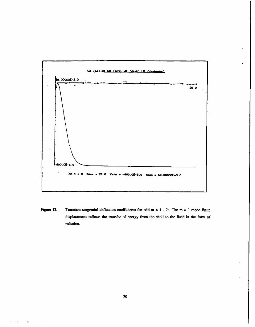
12 Transient tangential deflection coefficients for odd m = 1 - 7 ......................... 30

13 Early-time tangential displacements at three locations .................................. 31

14 Longer-time tangential displacements at five locations .................................. 32

15 Transient tangential velocities at three locations on the shell ......................... 33

16 Transient tangential accelerations at three locations ...................................... 34

17 Strains in theio-direction ......................................................................... 35

18 Strain rates in the # l-direction .................................................................. 36

19 Strains in the TI-direction ........................................................................ 37

20 Strain rates in theTI-direction ................................................................... 38

viii

LIST OF TABLES

Table Page

1 Physical constants .................................................................................. 6

2 Geometic parameters .............................................................................. 9

3 Nondimensionalized in vacuo natural frequencies. ........................................ 12

4 Dimensional in vacuo natural frequencies (kilohertz) .................................... 14

5 Nondimensionalized time versus real time (ins) ........................................... 18

ix

SECTION 1

INTRODUCTION

Structural acoustics is an area of mathematical physics which addresses the coupled fluid-solid

interaction between a structure and the fluid in which it is immersed. In fluid-solid interaction problems,

the analysis of the response of structures is coupled through the boundary conditions to the propagation of

energy in the fluid environment. It is incorrect to analyze an immersed structure independently of the fluid

medium, to analyze the fluid independently of a structure in its midst, and then to superimpose the

solutions. These problems require the simultaneous solution of the coupled field :•uations for both media

(Ref. 4, Chapter 1).

Because of the coupled nature of the problem, very few closed form solutions have been

developed. The problem of the shock response for a sphere in water was previously solved by Draper

(Ref. 1, 2). Numerical results were developed for a spherical shell structure which Draper was developing

for a different program. The numerical results were then compared with actual shock test results (Ref. 3).

The agreement was excellent.

Encouraged by these results, we attempted to extend the analysis to a prolate spheroidal shell

geometry. Unfortunately, this simple change in the geometry caused a very large increase in the difficulty

of the solution. Without the aid of computers, solution would be practically impossible.

However, computer programs are now available to help with the algebra involved with

manipulating the complex series expressions which result from attempts to solve this problem in closed

form. In particular, the DOE-MACSYMA program was used extensively to help in reducing the equations

to more reasonable forms.

SECTION 2

THEORETICAL DEVELOPMENT

The theoretical development of the equations is given in detail in Jones-Oliveira (Ref. 4). We

will present here only a brief summary of the steps involved.

The objective is to analyze the transient response of a prolate spherical shell structure which

has been externally loaded by an end-on explosive waterborne shock wave. The intention is to analyze the

effects of giving up one level of geometric symmetry (two degrees of symmetry for the prolate spheroid

versus three degrees of symmetry for the previous sphere analysis) (Ref. 4, Chapter 2).

Several simplifying assumptions are necessary to formulate a solution to this problem. It is

assumed that linear acoustic wave theory is sufficient to describe the propagation of the pressure field in the

water. This is a reasonable assumption except very near the explosive charge. Koiter-Sanders-Budiansky

theory for thin elastic shells is used for the formulation of the shell structure internal strain and kinetic

energy expressions (Ref. 4, Chapter 2). It is assumed that the fluid remains in contact with the shell at all

times (no cavitation). This will be true for reasonable explosive loads except very near the surface.

With these assumptions, the problem is linear. One set of differential equations describes the

motion of the fluid. A second set of differential equations describes the motion of the shell structure. The

two sets of equations are coupled by the requirement that the normal velocity and the pressure load are

matched at all times at the fluid-solid interface. The problem has thus been reduced to finding the solution

to these equations, a far from trivial task.

The problem is formulated in a prolate spheroidal coordinate system. The temporally and

spatially dependent shell displacement and fluid pressure fields are expressed modally in terms of the prolate

spheroidal angular functions of the first kind and a new set of prolate spheroidal radial functions of the first

and third kinds. The prolate spheroidal angular functions are shown to be solutions of both the acoustic

wave equation, which governs the fluid behavior, and the shell equilibrium equations. They are not the

eigenfunctions of the coupled fluid-structure problem. However, the solutions are exact within the limits of

using a finite numbers of terms of a infinite series to represent the solution (Ref. 4, Abstract).

The prolate spheroidal special functions are expressed in terms of classical spherical

harmonics: Specifically, Legendre polynomials and modified spherical Bessel functions of the first and

third kinds (Ref. 4, Abstract).

2

The mathematical physics governing the symmetry order two prolate spheroidal problem is

fundamentally different from that of the symmetry order three spherical problem previously solved. The

underlying geometric differences are at the Toot of the modal coupling, which is compounded by the fluid-

solid interaction at the interface. The totally uncoupled spherical response is a limiting case of the more

general and fully coupled prolate spheroidal response (Ref. 4, Chapter 2).

The modal coupling, which is not present in the spherical case, is the primary limitation to

obtaining practical solutions. If the coupling were not present, it would be reasonable to carry a large

number of terms in the series solutions. If the series converged very rapidly, it would not be too difficult to

solve the fully coupled problem using only a few terms in the series. Unfortunately, it appears that neither

is true.

DOE-MACSYMA was used extensively to determine the solution to this problem. The

capabilities of the symbolic computer code have been demonstrated to be invaluable for parametric analysis

(Ref. 4, Abstract). Unfortunately, the complexity of the resulting coupled functions is overwhelming, even

with DOE-MACSYMA. It became obvious that simplifications were imperative to achieve solutions

within the limitations of DOE-MACSYMA and reasonable total computer time. It was necessary to

estimate the relative magnitudes of each of the coupling terms to determine when terms could be neglected.

These simplifications must be considered judgement calls.

The coupling terms are more significant as the aspect ratio is increased. In principal, this is

not a limitation. As the aspect ration increased, one would just carry more terms in the solution. In

practice, this is subject to limitations:

1. Numerical precision of the calculations must also be increased to avoid round-off

erro.

2. Computer programs have size limits. In particular, DOE-MACSYMA can handle

large, but not unlimited, problems. This analysis was stretching its limits.

3. Computers have become faster and less expensive. However, problems which are

attempted have also grown. This problem might have been possible to solve to

higher accuracy by the use of much larger computer resources, but it would have

been prohibitively expensive to try.

3

SECTION 3

NUMERICAL RESULTS1

3.1 PHYSICAL AND GEOMETRIC PARAMETERS.

The physical constants are given in Table 1 on page 6. The fluid is taken to be fresh water,

and the shell material is steel.

The acoustic loading is that resulting from a sixty-pound spherical charge of HBX- I located at

a stand-off distance (S.O.D.) of 25 feet from the nose of the prolate spheroids. The peak external pressure2

of the incident pressure wave is given by

p = 2,347.6 (3.1)

and the exponential decay constant associated with the explosive charge is given by

[wi- •-0.247

S= 0.056W (~* 2 7 3)3 (S.O.D. (3.2)

where the explosive charge weight W is given in lbs and the stand-off distance S.O.D. is given inft. The

peak external pressure is expressed in terms of In& and the exponential decay constant is expressed inin2

terms of Ms.

1 Numerical calculations are presented for three representative prolate spheroidal geometries. The first

case models a "nearly spherical" geometry and is offered as verification of the correctness of the code by

comparing the results to the spencal analog. The second case models a 'Yoanded-off football." Preliminary

results are offered for a third case which models a "submarine-like" structure. The numerical complexities

are enormous. Limitations and comments are noted.

2 Formulas for the explosive characteristics are given in Jones-Oliveira (Ref. 4, Chapter 5.4).

4

2511wo N3X.1

S.O.O. 25 feetOpm 24 fIS

20OW

u1

cw

'1000

0 2 3 4 5 . . |

TIME (rol

Figure 1. Pressure versus time curve.

Table 1. Physical constants: This table provides the physical material properties used to generate the

numerical examples.

SYMBOL DEFINITION VALUE

exponential decay constant 0.3466 ms

c/ sound velocity in fluid 1498 S

CS sound velocity in shell 5404

c2nondmesianlize sound speed squared 13.0

E Young's modulus 2.11 x 101o-.!M 2

v Poisson's ratio 0.30

P peak external pressure given 1,883,966 M 2

60 # of HBX-1 at 25 ft S.O.D.

n nondimensionalized peak pressure 8.2406 x 10.3 Sdensity

of water 1.0188 x 102 gS2

m 4

density of shell 7.9385 x 102 kg-s2

m4

Sspecific weight of water m9 3

Ag specific weight of shell 7785m3

6

The geometric parameters associated with each of the three cases are given in Table 2 on page

9. In each case, a specific shell geometry was selected and sized, and the shell thickness was determined to

ensure a neutrally buoyant body.

The neutral buoyancy condition is defined such that the mass of the fluid displaced by the

prolate spheroid must equal tihe mass of the prolate spheroidal shell. The volume of a prolate spheroid is

given by V a I- x ab2 = 4 _ S (g2_1) (Ref. 4, Chapter 2.4.1). Clearly, the neutral buoyancy condition is

3 3a function of the nondimensionalized mass ratio, but it is also a function of the eccentricity. The

nondimensionalized shell thickness may be determined by solving the following cubic equation.

=7785 [(g + )(3 + L) )( • + (, -I)]

The remaining geometric parameters are then nondimensionalized as per (Ref. 4, Chapter 2.7).

Note that the nondimensionalizations of time differ for each of the three cases; therefore, so must the scaled

values of the incident pressure exponential decay constant f.

Case I: Model of a nearly spherical shell. The prolate spheroid has a low aspect ratio of 1.005 with

4o = 10.0. The pseudo-spherical parameters were selected to facilitate comparison to the spherical shell

which was modeled, tested and presented in Jones-Oliveira (Ref. 2). It should be noted that the parameters

are not identically those cited in Jones-Oliveira (Ref. 2); therefore, the results will be different. The shell

and fluid properties differ slightly; and the shell thickness was determined to ensure neutral buoyancy.

7

Case !1: Model of an intermediate aspect ratio geometry. Specifically, the aspect ratio is i- with e,4

also. The parameters were selected, for comparison purposes, to match as closely as possible those of

Pauwelussen (Ref. 7) and Nemergut & Brand (Ref. 6).

Case IiH: Model of a submarine-like structure. The prolate spheroid has a high aspect ratio of 10.0 and

= = 1.005. In particular, the geometry is similar to a small submersible currently being developed at The

Charles Stark Draper Laboratory.

Numerical results are also presented for a sphere which differs only slightly from the pseudo-

spherical problem. Its geometric parameters are those given for Case I with the following exceptions: [1]

the dimensional semifocal length is zero, = 0; [2] the semiminor axis length is equal to the semnimajor

axis length, b = and (31 the semimajor axis length is equal to the limiting value, 4f= a.

Table 2. Geometric parameters: This table provides the geometric paramet•s defining the three

illustrative examples. Case I refers to the low aspect ratio example, Case II refers to the

intermediate aspect ratio example, and Case M] refers to the high aspect ratio example.

CASE I CASE II CASE m

4 10.0000 1.4142 1.005

0.0323 m 1.4142 m 10.9182 m

a0.3239 m 2.0000 m 10.9728 m

b0.3222 m 1.4142 m 1.0932 m

O.G 147 m 0.0549 m 0.0074 m

h 4.5469 x 10-2 0.0275 6.7440 x 10'

AR 1.0050 1.4142 10.0375

e 0.1000 0.7071 0.995

h_ 1.7229 x 102 1.2554 x 10- 3.9 x 10'

121 2

M 2.8224 4.6761 189.4994

4,642.9251 t 749.0 t 136.5194 t

1.6091 0.2596 0.0473

wOn (hertz) 736.073191a. 119.20705fil 21.727740a

9

3.2 FREE VIBRATIONS OF PROLATE SPHEROIDS.

The first step in verifying the DOE-MACSYMA coding of the analysis was to compute the

free in vacuo vibrations of the three representative prolate spheroids. Included are the couplings of the

coefficients associated with the first eight Legendre polynomials. The spherical results are presented for

comparison purposes. The nondimensionalized results are tabulated in Table 3 on page 12 and the

dimensionalized frequencies are tabulated in Table 4 on page 14.

It is noted that the in vacuo natural frequencies of the pseudo-spherical prolate spheroid, i.e.,

Case I. for which 4 = 10.0 are within 1% of those computed for a sphere using the same parameters.

However, one would expect the frequencies of the sphere to be slightly higher than those of the prolate

spheroid. The discrepancies may be explained by the truncation of the infinite series iepresentations of the

prolate spheroidal angular functions expressed in terms of Legendre polynomals and/or by numerical errors

and/or by omission of the expansion coefficients.

Agreement of the first few modes of Case II, for which f = 1, is remarkable. Nemergut &

Brand (Ref. 6) computed an identical frequency for the lower branch of mode 2. In their paper, they compare

their own results with those of Shiraishi & DiMaggio (Ref. 8) and Silbiger & DiMaggio (Ref. 9).

The results for Case Ill for which 4z = 1.005, have to be considered somewhat suspect. The reasons for

concern are: [1] the lowest odd frequency is not close enough to zero; and [2] the branches cross each other.

Clearly, the rigid body translation, for which m = 1, should have a zero root. Normalization by the lowest"nonzero" frequency reveals cause for concern. Regarding the crossing of the branches, it is not known

whether or not these results are correct. Several options for further investigation are: [1] increase the

precision; [2] increase the number of modes that are allowed to couple; and/or [3] include the expansion

coefficients in the analysis.3 None of these suggestions is numerically trivial; however, the matter will be

addressed further.

3 As yet, the expansion coefficients in the numerics are all taken to be one. The assumption is that this

dependence will ultimately be absorbed into the time-dependent generalized displacements as per (Ref. 4,

Chapter 2.6.5).

10

It should be noted that there are, in fact, two branches; i.e., two natural frequencies associated

with each mode number. Please refer to Figure 2 on page 13, which plots the dimensional frequencies as a

function of mode number for Cases I & II. This phenomenon is an inherent characteristic of axisymmetric

shell structures. The simultaneous solution of the homogeneous system of partial differential equations,

which governs the normal and tangential deflections of shells of revolution, reduces to the solution of a

quartic equation; specifically, it is bi-quadratic. Except for the pure breathing mode m= 0, there result two

sets of nontrivial roots to the frequency determinant resulting in a bifurcation into a lower branch and an

upper branch (Ref. 5, Chapter 8). The m = 0 is a special case; it has only a single complex-conjugate pair

of roots because u, 0.

t.2

The lower branch appears to contain the - parameter and is, therefore, sensitive to bending12ý

stiffness. On the other hand, the upper branch is relatively insensitive to bending stiffness. If one were to

model only the extensional vibrations of the prolate spheroidal shell, which would imply that the I"

12nterms were omitted, then the frequencies on the lower branch would be too low but the frequencies on the

upper branch would not be affected appreciably.

Finally, all of the even (odd) normal displacements are coupled to all of the even (odd)

tangential displacements. Therefore, it is not possible, a priori, to discern which frequency (lower or upper

branch) is associated with which displacement. It is conjectured that the lower branch may be dominated by

the tangential displacements.

11

Table 3. Nondimensionalized in vacuo natural frequencies.

SPHERE PROLATE SPHEROID

Case I Case II Case III

mode r 4 = 1o.o f2 go = 1.oo5

1 0.0 0.0 0.0049 2.7448

2 2.5325 2.5492 3.7592 7.7304

3 3.0252 3.0470 4.6356 12.9879

4 3.2799 3.3039 4.9566 17.9642

5 3.5125 3.5385 5.2955 23.4785

6 3.8030 3.8311 5.5944 28.4777

7 4.1922 4.2232 6.2635 37.3266

8 4.7012 4.7358 6.6211 36.9838

0 5.8138 5.8332 7.1347 41.6152

1 7.1210 7.1544 9.5473 39.1475

2 9.8168 9.8457 12.3497 44.4057

3 13.1101 13.1445 15.7277 48.1471

4 16.5785 16.6207 19.5272 52.5743

5 20.1094 20.1602 23.5383 73.3820

6 23.6685 23.7281 27.6355 81.2022

7 27.2426 27.3113 32.8058 198.7833

8 30.8255 30.9032 37.2074 218.9494

12

Um

16

16

14

12

10

8

6

4

2_

1 2 3 4 5 6 7 8 9 10 m

IN VACUO NATURAL FREO. VS. MODE 6

- SPHERE. - 10.0

Figure 2. Dimensional Frequency versus mode number.

13

Table 4. Dimensional in vacuo natural frequencies (kilohertz).

SPHERE PROLATE SPHEROID

Case I Case H Case III

mode r o = 1o.o = o = 1.oo5

1 0.0 0.0 5.8412 x 10' 0.0596

2 1.8639 1.8764 0.4481 0.1680

3 2.2265 2.2428 0.5526 0.2822

4 2.4140 2.4319 0.5909 0.3903

5 2.5852 2.6046 0.6313 0.5101

6 2.7990 2.8200 0.6669 0.6188

7 3.0854 3.1086 0.7467 0.8109

8 3.4601 3.4859 0.7893 0.8036

0 4.2789 4.2937 0.8720 0.9042

1 5.2411 5.2662 1.1381 0.8506

2 7.2252 7.2472 1.4722 0.9648

3 9.6491 9.6753 1.8749 1.0461

4 12.2018 12.2341 2.3278 1.1423

5 14.8005 14.8394 2.8059 1.5944

6 17.4200 17.4650i 3.2943 1.7643

7 20.0506 20.1031 3.9107 4.3191

8 22.6876 22.7470 4.4354 4.7573

14

3.3 FLUID.LOADED VIBRATIONS.

In order to solve the even-even/odd-odd coupled equations for the fluid-loaded natural

frequencies, it is necessary to simplify the equations. Here, the emphasis is on the "coupling" of the

coefficients in the differential equations resulting from the Legendre polynomials representation. The

trimming procedure is as follows:

1. Inspect the coefficients of each displacement appearing in the left-hand side of each

of the modal equations given by (Ref. 4, 3.5.2a & 3.5.2b). Normalize the

coefficients by the nth coefficient of the displacement in the nth equation. Let each

normalized coefficient which is less than 0.0001 be set to 0.0. Allow an additional

order of magnitude for each power of s (since the observed range of s satisfies

Is I < 20).

2. Note that the coupling terms at the fluid-solid interface appearing on the right-hand

side of equation (Ref. 4. 3.5.2a) (see also Ref. 4, 3.3.5.4) have a factor of bni x

brm. Each of these coefficients drops off rapidly as the mode numbers increase, so

their products drop off even faster. Practically, this means that the inner summation

in the numerator of (Ref. 4. 3.3.5.4) is not infinite; in fact, in most cases, only the

diagonal elements survive the trimming procedure. In other words, only the (bnm)2

terms usually survive.

3. When necessary and appropriate, back-substitute the solutions for the lower modes

into the equations for the higher modes to solve for the higher modes.

These simplifications are necessary in order to compute the solution effectively. Otherwise,

the order of the polynomials which must be solved exceeds the capabilities of the root solvers. For

example, consider Case I for which 0 = 10. Without these simplifications, the order of the polynomial

for solving the coupling of wo, u2, w", u , and w4 is 64 and the DOE-MACSYMA ALLROOTS solver

was only able to fund 14 of the roots. The polynomials become ill-conditioned.

15

It was verified that the roots are quite stable against this trimming procedure. For the smaller

problem, which models the the most significant cross-coupling, specifically that associated with the lowest

modes (w", u2 and w2), the roots moved by less than 1% with these simplifications. This smaller problem

could be solved exactly and the results were used for the verification.

The characteristic roots are presented in the form

S = -a±Qi

where s = Laplace variable

-a = tenuation

S= nondimensionalized damped natural fequiency.

The first few roots for Case I, for which , f 10.0, are

m = 0: Wo, M ON0

s=- 1.940

s = - 1.366 5.400i

iM = : W1dgl

s= 0

s = - 1.526 0.918i

s = - 0.887 + 6.830i

= : 2: w2, U2

s = - 1.097

s = - 1.940

s = - 3.052

16

s-- 1.9101 2.455i

s =-0.1306± 1.785i

s= -2.692 1.779i

s =-.403 9.701i

3.4 SHOCK-LOADED VIBRATIONS.

The characteristic roots for the shock-loaded problem are identical to the roots given for the

fluid-loaded homogeneous problem with the addition of a root associated with the shock. Specifically, there

is an additional real root s = -1.609.

The nondimensionalized normal and tangential displacements for the shock-loaded submerged

shell amre plotted as a function of nondimensionalized time. The dimensional deflections may be determined

from the nondimensionalized values by multiplying by the kg factors for the given geometry: Case I for

which 40 = 10.0, 4j= 0.323; Case II for which to = ý2, kf= 2.0; and Case III for which

to = 1.005, tf-= 10.97

Similar conversions may be used to obtain the physical dimensional velocities and

accelerations. Refer to Table 5 on page 18 as necessary to relate nondimensionalized time r to real time t.

17

Table 5. Nondimensionalized time versus real time (ms).

1r Cmel C.mli CmlU

S= 0.0 /2- = 1 .oo5

0 0.0 0.0 0.0

1 0.215 1.335 7.325

2 0.431 2.670 14.650

3 0.646 4.005 21.975

4 0.162 5.341 29.300

5 1.077 6.676 36.625

10 2.154 13.351 73.250

15 3.231 20.027 109.175

20 4.301 26.702 146.500

25 5.395 33.379 133.124

30 6.461 40.053 219.749

35 7.538 46.729 256.374

40 L615 53.405 292.999

45 9.692 60.080 329.624

50 10.769 66.756 366.248

60 12.923 80.107 439.493

70 15.077 93.451 512.743

s0 17.231 106.309 585.997

90 19.334 120.160 659.247

100 21.538 133.511 732.497

110 23.692 146.U63 805.763

120 25.346 160.214 378.996

130 21.000 173.565 952.246

140 30.153 136.916 1025.495

150 32.307 200.267 1098.745

18

3.4.1 Case I: Low Aspect Ratio.

Figure 3 on page 21 through Figure 16 on page 34 are DOE-MACSYMA-generated plots of

the normal and tangential generalized displacements (i.e., the time-dependent amplitudes), normal and

tangential physical displacements, velocities and accelerations for the low aspect ratio geometry in response

to the specified underwater explosion.

The following observations were made.

"The rigid-body generalized displacements (modal time-dependent amplitudes), w 1.

and ul, indicate a finite displacement of the shell. This may be explained as

follows. Recall that the generalized forces are the superposition of the incident,

scattered and radiated pressure waves in the fluid. The incident shock wave imparts a

force onto the prolate spheroidal shell and continues past the shell. Scattered energy

is reflected off the shell back into the fluid. Radiated energy is also put back into

the fluid due to the motion of the shell through the fluid, which can also re-load the

structure. The loss of energy to the fluid, once the exponentially decaying incident

shock wave has passed the prolate spheroid (r> 2), damps the motion of the shell

as it moves through the fluid resulting in the finite displacement.

" It is also noted that max (w2) >> max (xo). This means that w2 is strongly

coupled to wo but not vice versa. The equations coupling "0, U2. and wv reveal that

wo has both of the roots for m = 0 and the fourth root for m = 2, which points out a

strong coupling to u2. This can be deduced because this fourth m = 2 root is the

extra root associated with u2, which is predicted by the analysis and comparison to

the spherical problem.

* maxa (i) max m , .max (w) andmax (w3) >> max ws), max (w),...

19

* u5 drops off rapidly as n increases.

"* As the mode number increases, the couplings become negligible.

" As time progresses, the displacements can be seen to damp out and then to re-excite

as the fluid and shell motions exchange their energy through the kinematic boundary

conditions at the fluid-solid interface.

" The number of modes required to model the response adequately was determined by

examining the accelerations, rather than by considering just the relative magnitudes

of the displacement coefficients. It was determined that the acceleration contributed

by the 7 th mode was less than 10% of the total acceleration contributed by modes

m = 0 - 6. A better criterion could be established by examining the conservation of

energy of the system. Acceleration information is of keen interest to experimental

engineers because these predictions can be verified directly using accelerometers.

The shell strains, as defined by (Ref. 4, 3.1.1.5), and strain rates are presented in Figure 17 on

page 35 through Figure 20 on page 38. Again, the strain information is of interest to experimental

engineers because strain gauge readings are easily obtained. Comparisons of predicted values versus

empirical data may be accomplished using the square root sum of the squares.

20

)0.00009-3.0

.OE-3.0 ~

X~min n 0 Yaxu a 20.0 Yonam -SW.C0.E-3.0 Yin.. a 300.0000E-3-0

W. . ... ... - WS

-- .', -- W",, --- - -----------,-,-.-- W7

... ... ......". - W 3-" '

-. - W 4

Figure 3. Modal time-dependent normal amplitudes for m = 0 - 7: With the exception of component

m=l, the generalized displacements return to their original equilibrium position. However,

the mn = 1 contribution results in a finite displacement of the shell.

21

250.00001-3.0

I'I

Xmi 0 XWz -20.0 e'nae = -2S0.CE-3.0 Y-a 250.0000E-3.0

Figure4. Transient normal deflecon coefficientsforeven -6: Note atthe 2 mode has

dhe most significant amplitude. This explains its strong coupling to the lower even modes.

22

U, U•I .i~ ,• fdael U• Cdk U'? (damh-dint

600. OE-3.

Xmi• a 0 Yona, .20.0 Yein -O0.0.3.0 Ym ; a 200..O ..E.3. 0

Figure 5. Transient normal deflection coefficients for odd m = I - 7: The m = 1 mode finite

displacement reflects the transfer of energy from the shell to the fluid in the form of

radiation.

23

o .024.0

i I t I - S

• ./ ~."•,.................

L4.1.0-3.0

Uin - 0 Xm. a 20.0 Ymin a -4.0E-3.0 Yun - 10.01-3.0

71= + 1.0--- -- + 0.6

.................... 10.0"---1 i,. 0.6

"-- -- " 1.0

Figure 6. Early-time normal displacements at five locations on the shell: The positions vary from the

nose to the back side relative to the shock.

24

o.E-3,.0

50.

iI,

# mI a 0 a a St.0 I a *I % I • • I I t I s

TI M +' 1.

* , ,~ I, *

.......... I M00.0

E.(:-3 .0

-ll 0 Xau ,, 50.0 Yami - -4.OE-3.O yam, ,, I0.OE-3.0

1= + 1.0

- - Tin= 0.6m m.* ?1g 0.0

"- 11= - 0.6

-- -'I. 1.0

Figure 7. Longer-time normal displacements at five locations on the shell: Note the oscillation of the

displacement amplitudes-first dying out and then re-exciting.

25

I.OE-3.0

I -\I

Xm;n ,, 0 Xau ,, 20.0 Ymin - -10.0E-3.0 Ymau• , 10.01-3.0

11,, 1.011= + 0.6

S... ... ... ... ... 1= 0.0"--1 = - 0.6

S. .. . .. . 11=- 1.0

Figure 8. Transient normal velocities at five locations on the shell: Additional data points would

smooth out the plots.

26

.000001-3.0

Xamn * C Ximu - 20.0 Ymn - -25.01-3.0 Yux- 20.000001-3.0

I1= + 1.0Tlin +a 0.6

............... 16=0.0________ - '1- 0.6- ~ ~ ~ T .. - -- 1.0

Figure 9. Transient normal accelerations at five locations on the shell: Additional points would

smooth out the plots.

27

00OE-3.0

Xmin a 0 Xn.m m 20.0 Ymin w -600.OE-3.0 Y"K. a 100.OE-3.0

Leged

• . I - . - Us

U 2 U 6

----- -- -- ---- U 3 U 7

..*... .....

U

Figure 10. Modal time-dependent tangential amplitudes for m 1 - 7: With the exception of

component m = 1, the generalized displacements return to their original equilibriu n

position. However, the m = I contribution results in a finite displacement of thc shell.

Note that m = 0 is zero by definition.

28

,0. -3.0

XAin ,a 0 X... a 20.0 Ymin -.-60.O-3.0 Y. a- 60.000O00-3.0

Figure 11. Transient tangential deflection coefficients for even m = 2 - 6: Note that the m = 2 mode

has the most significant amplitude. This explains its strong coupling to the lower even

modes.

29

I.I teal ;d' Lfl (dn.1 L[K fi'.h1 [1'7 ¢,,,r- -

lO.000OW•-3.O .

20.0

4600.OE-3.0

xmin 0 0 X•as , 20.0 Ywin -400.0E-3.0 Ymea SO.O000019 -3.0

Figure 12. Transient tangential deflection coefficients for odd m = I - 7: The m = 1 mode finite

displacement reflects the transfer of energy from the shell to the fluid in the form of

radiation.

30

10.0000E-G .0

20.0

hS -SE-3.O0

Xmin -0 Xmas 20.0 Ymi" -9-.SE-3.0 YUs. SOO.~OCOE....o

Figure 13. Early-time tangential displacements at three locations: The tangential displacements at thetwo vertices are zero.

31

TA.MJlAAd P~t.. * _* (.1 iiq 6 Vdk~t• - A (,4-h1

50.0

-s. sE-3.0

X-in a • XKwe . 50.0 Yuin , -6.5E-3.0 Yin.. lSA00.O0OE-6.0

Figure 14. Longer-time tangential displacements at five locations: Note the oscillation of the

displacement amplitudes-first dying out and then re-exciting, albeit to a lesser extent than

was the case for the normal displacements.

32

TA#. WE F• -m _ tutmlId 0 t -• A fdI~h•

iv .V,. %,,

I I

-lr

'I

'I

Xan ,, 0 XmA ,, 20.0 Yein a -3.SE-3.0 Ymax a 1.5000OOE-3.0

Figure 15. Transient tangential velocities at three locations on the shell: Additional data points would

smooth out the plots.

33

.000001E-3.0

11

.10,(E-3.0

Xain a 0 Xnau o 20.0 Y'ein a -10.01-3.0 Ym a 8- .000001E-3.0

Figure 16. Transient tangential accelerations at three locations: Additional data points would smooth

out the plots, and perhaps slightly increase the maximum values.

34

m final ;� p fdat'� .. 1 f�a.h'l

'� i I!

I 4-3.0

Xman - 0 Xmmu - 20.0 Ymia - -1.4-3.0 Yam. - 1.200000E-3.0

Figure 17. Suiins in die 4�-direcuon.

35

EPSIIRATWFt V- . dh0fe -t*I

AA

*I Ij 3..0

Y-in -0 Xe.. - 20.0 lmine -3.CE-3.0 YiNOR 2- 2OOOOOE-3.o

Figure 18. Surain rates in the 41-direction.

36

a ¶ pal d~0(clot) .1 fd.ahh

a-.200E-3 .0

Xmin -0 Xomu- 20.0 Ymin - -. 2E-3.O Younal .2C00000-3.0

Figure 19. Strains in the 71-direction.

37

-3.0

vi II 0l•

X a in , 0 X ma • , 2 0 .0 .Ym in * - 2 .S E - 3 .0 Y m' z - 2 .5 0 0 0 0 0E - 3 .0

Figure 20. Srain rates in the il-direction.

38

3.4.2 Case 11 and Case IIL.

Reasonable numerical results could not be obtained for these cases. We believe that this did

not result from a fundamental flaw in the theory. Rather, it is because the series solutions do not converge

as fast as the aspect ratio is increased. In addition, cross-coupling terms which were negligible in the first

case are more important in these cases. If the model size that DOE-MACSYMA could handle were

increased and more computer power were used, solution should be possible. This is not currently practical.

However, as computer power expands in the future, it should become more reasonable.

39

SECTION 4

CONCLUSIONS

In order to solve the prolate spheroidal fluid-solid interaction problem, it was necessary to

balance classical analysis and numerical code development. Separation of the prolate spheroidal wave

equation reveals the prolate spheroidal angular and radial functions to be the exact solutions to the prolate

sp1meoidal acoustic wave equation, as expected. The prolate spheroidal angular functions are also determined

to be eigen solutions for the prolate spheroidal shell equilibrium equations. The shell displacement and

fluid pressure fields are expressed in terms of an infinite series expansion using the complete set of prolate

spheroidal angular functions and are therefore exact. The resulting expressions are very complex (Ref. 4,

Chapter 5). However, DOE-MACSYMA was very helpful in dealing with the complex algebraic

manipulations.

The final result was an exact solution for the transient response of both the prolatc spheroidal

shell and the surrounding fluid medium. However, the results are represented in terms of infinite series,

embedded in infinite series, embedded in infinite series, etc. Computationally, such a representation is very

difficult to deal writh (Ref. 4, Chapter 5).

A novel trimming procedure, which was guided by the functional insight gained in the

analysis, was required to solve for numerical answers. This trimming procedure was sufficient to obtain

shock-loaded results for the nearly-spherical prolate spheroidal geometry (Ref. 4, Chapter 5). For this case,

the results were compared with the results previously generated for the perfect sphere and the agreement was

excellent.

Unfortunately, this procedure was not sufficient to obtain valid solutions for the higher

eccentricity geometrics. One of the primary problems for the eccentric geometries is modal coupling.

Unfortunately, the fact that the resulting series solutions are separately solutions to the wave equations and

the shell equations does not mean that they are normal eigenfunctions which would uncouple the equations.

Theoretically, a set of normal eigenfunctions exist which would uncouple the equations. However, it is not

known how to find such a set of functions.

In principal, the equations can be evaluated in spite of the cross-coupling. However, it was

determined that the higher the eccentricity, the slower the power series converged and the more significant

the coupling of the modes. For practical solution with currently reasonable computer resources, the cross-

coupling terms must be dropped and the series truncated at a reasonable number of terms. Unfortunately,

this results in incorrect answers. In the future, increased computer power may make this

40

solution useful in an engineering sense. However, at this time the method can not be used to solve

practical problems.

Since reasonable numerical solutions could not be obtained for high eccentricity geometries

using the new closed-form theory, we were unable to compare the new theory with experimental or finite

element results.

41

SECTION S

LIST OF REFERENCES

1. Huang, Hanson, "Transient Interaction of Plane Acoustic Waves with a Spherical Elastic

Shell," Journal of the Acoustical Society of America, Volume 45, No. 3, March 1969,

pp. 661-670. (Unclassified)

2. Jones-Oliveira, Janet B., "Transient Interaction of Plane Acoustic Waves with Submerged

Elastic Spherical Shells," Master of Science Thesis, Massachusetts Institute of Technology,

CSDL-T-846, Revision A, June 1984. (Unclassified)

3. Jones-Oliveifa, Janet B., and Peter J. Wender, "Explosive Shock Analysis and Test of a Sonar

Towed Body," CSDL-P-1981, December 1984 [also published in The 55th Shock and

Vibration Bulletin]. (Unclassified)

4. Jones-Oliveira, Janet Bughardt, "Fluid-Solid Interaction of a Prolate Spheroidal Shell Structure

by an Acoustic Shock Wave," Doctoral Thesis, Massachusetts Institute of Technology, March

1990. (Unclassified)

5. Kraus, Harry, "Thin Elastic Shells," John Wiley and Sons, Inc., New York, NY, 1967,

pp. 333-341. (Unclassified)

6. Nemergut, PJ., and R.S. Brand, "Axisymmetric Vibrations of Prolate Spheroidal Shells,"

Journal of the Acoustical Society of America, Volume 38, 1965, pp. 262-265. (Unclassified)

7. Pauwelussen, Poop P., "Validation of the Underwater Shock Analysis Program USA," Part II:

Numerical Computations, Institute for Mechanical Constructions, January 1987. (Unclassified)

8. Shiraishi, N., and Frank L. DiMaggio, "Perturbation Solution for the Axisymmetric

Vibrations of Prolate Spheroidal Shells," Journal of the Acoustical Society of America,

Volume 34, 1962, pp. 1725-1731. (Unclassified)

9. Silbiger, Alexander, ,nd Frank DiMaggio, "Extensional Axi-Symmetric Second Class

Vibrations of a Prolate Spheroidal Shell," Office of Naval Research, Contract Nonr-266(67),

Project 385-414, Technical Report No. 3, February 1961. (Unclassified)

42

DISTRIBUTION LIST

DNA-TR-90-171

DEPARTMENT OF DEFENSE ATTN: CODE 1750ATTN: CODE 1770

ASSISTAN• TO THE SECRETARY OF DEFENSE ATTN: CODE 2740ATTN: EXECUTIVE ASSISTANT

MARINE CORPSDEFENSE INTELLIGENCE AGENCY ATTN: CODE POR-21

ATTN: DB-6E1ATTN: DIW-4 NAVAL COASTAL SYSTEMS CENTERATTN: OGA-4B2 ATTN: CODE 7410

DEFENSE NUCLEAR AGENCY NAVAL DAMAGE CONTROL TRAINING CENTERATTN: OPNS ATTN: COMMANDING OFFICERATTN: SPSDATTN: SPWE NAVAL ELECTRONICS ENGRG ACTVY, PACIFICATTN: SPWE K PETERSEN ATTN: CODE 250

2 CYS ATTN: TITL NAVAL EXPLOSIVE ORD DISPOSAL TECH CENTER

DEFENSE TECHNICAL INFORMATION CENTER ATTN: CODE 90 J PETROUSKY2 CYS ATTN: DTICIFDAB NAVAL POSTGRADUATE SCHOOL

FIELD COMMAND DEFENSE NUCLEAR AGENCY ATTN: CODE 1424 LIBRARYATTN: FCPR NAVAL RESEARCH LABORATORY

FIELD COMMAND DEFENSE NUCLEAR AGENCY ATTN: CODE 2627 TECH LIBATT'N: FCNV NAVAL SEA SYSTEMS COMMAND

FIELD COMMAND DEFENSE NUCLEAR AGENCY ATTN: SEA-08ATTN: FCNM ATTN: SEA-423

ATTN: SEA-511DEPARTMENT OF THE ARMY ATTN: SEA-55X1

ATTN: SEA-55YDEP CH OF STAFF FOR OPS & PLANS

ATTN: DAMO-SWN NAVAL SURFACE WARFARE CENTERATTN: CODE H21

HARRY DIAMOND LABORATORIES ATTN: CODE R14ATTN: SLCIS-IM-TL TECH LIB ATTN: CODE R15

U S ARMY CORPS OF ENGINEERS NAVAL WEAPONS CENTERATTN: CERD-L ATTN: CODE 3241 D HERIGSTAD

U S ARMY ENGR WATERWAYS EXPER STATION NAVAL WEAPONS EVALUATION FACILITYATTN: CEWES J K INGRAM ATTN: CLASSIFIED LIBRARYATTN: CEWES-SD/DR J G JACKSON, JRATTN: J ZELASKO CEWES-SD-R NEW LONDON LABORATORYATTN: R WHALIN CEWES ZT ATTN: TECH LIBRARYATTN: RESEARCH LIBRARY

OFFICE OF CHIEF OF NAVAL OPERATIONSU S ARMY NUCLEAR & CHEMICAL AGENCY ATTN: NOP 091

ATTN: MONA-NU DR D BASH ATTN: NOP 223ATTN: NOP 225

U S ARMY SPACE & STRATEGIC DEFENSE CMD ATTN: NOP 37ATTN: CSSD-SA-EV ATTN: NOP 605D5ATTN: CSSD-SL ATTN: NOP 957E

U S ARMY WAR COLLEGE ATTN: OP 03EGATTN: OP 21ATTN: LIBRARY ATTN: OP 654

USA SURVIVABILITY MANAGMENT OFFICE ATTN: OP 73 TAC READINESS DIVATTN: SLCSM-SE J BRAND OFFICE OF NAVAL RESEARCH

DEPARTMENT OF THE NAVY ATTN: CODE 11 32SMATTN: CODE 23

DAVID TAYLOR RESEARCH CENTERATTN: CODE 172 DEPARTMENT OF THE AIR FORCEATTN: CODE 173 AIR FORCE INSTITUTE OF TECHNOLOGY/ENATTN: CODE 1740 ATTN: COMMANDER

Dist-1

DNA-TR-90-171 (DL CONTINUED)

HO USAF/CCN COLUMBIA UNIVERSITYArTTN: AFCCN ATTN: F DIMAGGIO

UNITED STATES STRATEGIC COMMAND KAMAN SCIENCES CORPATTN: J 51 ATTN: LIBRARYATTN: J 533ATTN: J 534 KAMAN SCIENCES CORP

ATTN: J 535 ATTN: DASIACATTN: E CONRAD

DEPARTMENT OF ENERGYKAMAN SCIENCES CORPORATION

LAWRENCE LIVERMORE NATIONAL LAB ATTN: DASIACATTN: D MAGNOLI

KARAGOZIAN AND CASELOS ALAMOS NATIONAL LABORATORY ATTN: J KARAGOZIAN

ATTN: REPORT LIBRARYATTN: TECH LIBRARY LOCKHEED MISSILES & SPACE CO. INC

ATTN: PHILIP UNDERWOODMARTIN MARIETTA ENERGY SYSTEMS INC

ATTN: DR C V CHESTER LOCKHEED MISSILES & SPACE CO, INCATTN: TECH INFO CTR

SANDIA NATIONAL LABORATORIESATTN: TECH LIB 3141 PACIFIC-SIERRA RESEARCH CORP

ATTN: H BRODEU S DEPARTMENT OF ENERGYOFFICE OF MILITARY APPLICATIONS S-CUBED

ATTN: OMAIDP-252 MAJ D WADE ATTN: K D PYATT. JRATTN: R SEDGEWICK

OTHER GOVERNMENTSCIENCE APPLICATIONS INTL CORP

CENTRAL INTELLIGENCE AGENCY ATTN: TECHNICAL REPORT SYSTEMAT'ITN: OSWR/NED

TELEDYNE BROWN ENGINEERINGDEPARTMENT OF DEFENSE CONTRACTORS ATTN: J RAVENSCRAFT

ANALYSIS & TECHNOLOGY INC TITAN CORPORATIONATTN: V GODINO ATTN: LIBRARY

ATTN: S SCHUSTERAPPLIED RESEARCH ASSOCIATES, INC

ATTN: R FRANK WEIDLINGER ASSOC. INCATTN: H LEVINE

CALIFORNIA INSTITUTE OF TECHNOLOGYATTN: T AHRENS WEIDLINGER ASSOCIATES, INC

ATTN: T DEEVYCALIFORNIA RESEARCH & TECHNOLOGY, INC

ATTN: J THOMSEN WEIDLINGER ASSOCIATES, INCATTN: K KREYENHAGEN ATTN: M BARON

CHARLES STARK DRAPER LAB, INC WESTINGHOUSE ELECTRIC CORP2 CYS ATTN: D S NOKES ATTN: D BOLTON ADV DEVELOP

Dist-2