ActiveClean: Interactive Data CleaningFor Statistical Modeling

Sanjay Krishnan, Jiannan Wang †, Eugene Wu ††, Michael J. Franklin, Ken GoldbergUC Berkeley, †Simon Fraser University, ††Columbia University

{sanjaykrishnan, franklin, goldberg}@berkeley.edu jnwang@sfu.ca ewu@cs.columbia.edu

ABSTRACTAnalysts often clean dirty data iteratively–cleaning some data, ex-ecuting the analysis, and then cleaning more data based on the re-sults. We explore the iterative cleaning process in the context ofstatistical model training, which is an increasingly popular form ofdata analytics. We propose ActiveClean, which allows for progres-sive and iterative cleaning in statistical modeling problems whilepreserving convergence guarantees. ActiveClean supports an im-portant class of models called convex loss models (e.g., linear re-gression and SVMs), and prioritizes cleaning those records likelyto affect the results. We evaluate ActiveClean on five real-worlddatasets UCI Adult, UCI EEG, MNIST, IMDB, and Dollars ForDocs with both real and synthetic errors. The results show that ourproposed optimizations can improve model accuracy by up-to 2.5xfor the same amount of data cleaned. Furthermore for a fixed clean-ing budget and on all real dirty datasets, ActiveClean returns moreaccurate models than uniform sampling and Active Learning.

1. INTRODUCTIONStatistical models trained on historical data facilitate several im-

portant predictive applications such as fraud detection, recommen-dation systems, and automatic content classification. In a survey ofApache Spark users, over 60% responded that support for advancedstatistical analytics was Spark’s most important feature [1]. Thissentiment is echoed across both industry and academia, and therehas been significant interest in improving the efficiency of modeltraining pipelines. Although it is often overlooked, an importantstep in all model training pipelines is handling dirty or inconsistentdata including extracting structure, imputing missing values, andhandling incorrect data. Analysts widely report that cleaning dirtydata is a major concern [21], and consequently, it is important tounderstand the efficiency and correctness of such operations in thecontext of emerging statistical analytics.

While many aspects of the data cleaning problem have beenwell-studied for SQL analytics, the results can be counter-intuitivein high-dimensional statistical models. For example, studies haveshown that many analysts do not approach cleaning as a one-shot

This work is licensed under the Creative Commons Attribution-NonCommercial-NoDerivatives 4.0 International License. To view a copyof this license, visit http://creativecommons.org/licenses/by-nc-nd/4.0/. Forany use beyond those covered by this license, obtain permission by emailinginfo@vldb.org.Proceedings of the VLDB Endowment, Vol. 9, No. 12Copyright 2016 VLDB Endowment 2150-8097/16/08.

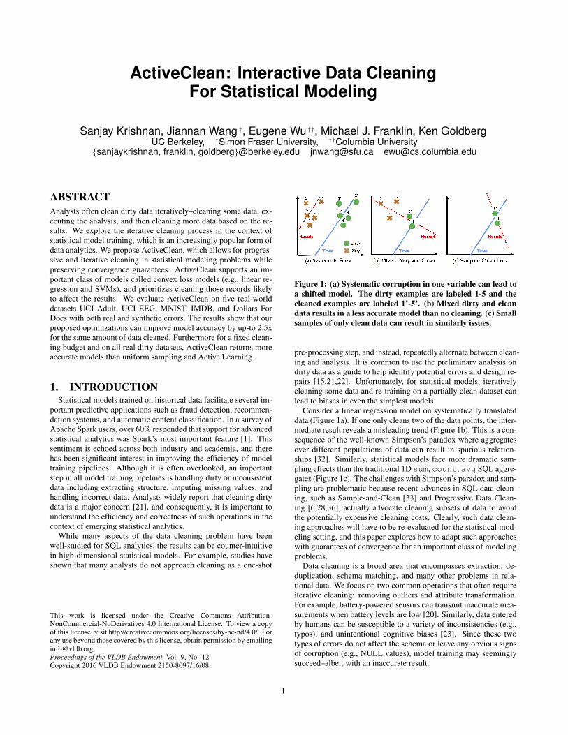
Figure 1: (a) Systematic corruption in one variable can lead toa shifted model. The dirty examples are labeled 1-5 and thecleaned examples are labeled 1’-5’. (b) Mixed dirty and cleandata results in a less accurate model than no cleaning. (c) Smallsamples of only clean data can result in similarly issues.

pre-processing step, and instead, repeatedly alternate between clean-ing and analysis. It is common to use the preliminary analysis ondirty data as a guide to help identify potential errors and design re-pairs [15,21,22]. Unfortunately, for statistical models, iterativelycleaning some data and re-training on a partially clean dataset canlead to biases in even the simplest models.

Consider a linear regression model on systematically translateddata (Figure 1a). If one only cleans two of the data points, the inter-mediate result reveals a misleading trend (Figure 1b). This is a con-sequence of the well-known Simpson’s paradox where aggregatesover different populations of data can result in spurious relation-ships [32]. Similarly, statistical models face more dramatic sam-pling effects than the traditional 1D sum, count, avg SQL aggre-gates (Figure 1c). The challenges with Simpson’s paradox and sam-pling are problematic because recent advances in SQL data clean-ing, such as Sample-and-Clean [33] and Progressive Data Clean-ing [6,28,36], actually advocate cleaning subsets of data to avoidthe potentially expensive cleaning costs. Clearly, such data clean-ing approaches will have to be re-evaluated for the statistical mod-eling setting, and this paper explores how to adapt such approacheswith guarantees of convergence for an important class of modelingproblems.

Data cleaning is a broad area that encompasses extraction, de-duplication, schema matching, and many other problems in rela-tional data. We focus on two common operations that often requireiterative cleaning: removing outliers and attribute transformation.For example, battery-powered sensors can transmit inaccurate mea-surements when battery levels are low [20]. Similarly, data enteredby humans can be susceptible to a variety of inconsistencies (e.g.,typos), and unintentional cognitive biases [23]. Since these twotypes of errors do not affect the schema or leave any obvious signsof corruption (e.g., NULL values), model training may seeminglysucceed–albeit with an inaccurate result.

1

We propose ActiveClean, a model training framework that al-lows for iterative data cleaning while preserving provable conver-gence properties. The analyst initializes ActiveClean with a model,a featurization function, and a pointer to a dirty relational table. Ineach iteration, ActiveClean suggests a sample of data to clean basedon the data’s value to the model and the likelihood that it is actuallydirty. The analyst can apply value transformations and filtering op-erations to the sample. ActiveClean will incrementally and safelyupdate the current model (as opposed to complete re-training). Wepropose several novel optimizations that leverage information fromthe model to guide data cleaning towards the records most likely tobe dirty and most likely to affect the results.

From a statistical perspective, our key insight is to treat the clean-ing and training iteration as a form of Stochastic Gradient Descent,an iterative optimization method. We treat the dirty model as an ini-tialization, and incrementally take gradient steps (cleaning a sampleof records) towards the global solution (i.e., the clean model). Ouralgorithm ensures global convergence with a provable rate for animportant class of models called convex-loss models which includeSVMs, Linear Regression, and Logistic Regression. Convexity isa property that ensures that the iterative optimization converges toa true global optimum, and we can apply convergence argumentsfrom convex optimization theory to show that ActiveClean con-verges.

To summarize our contributions:

• We propose ActiveClean, which allows for progressive datacleaning and statistical model training with guarantees.• Correctness We show how to update a dirty model given

newly cleaned data. This update converges monotonically inexpectation with a with rate O( 1√

T).

• Optimizations We derive a theoretically optimal samplingdistribution that minimizes the update error and an approxi-mation to estimate the theoretical optimum. We further showthat ActiveClean can integrate with existing dirty data de-tection techniques. Our proposed optimizations can improvemodel accuracy by up-to 2.5x for the same amount of datacleaned.• Experiments The experiments evaluate ActiveClean on five

datasets with real and synthetic corruption. In a fraud predic-tion example, ActiveClean examines nearly 10x less recordsthan alternatives to achieve an 80% true positive rate.

The correctness of many of the components detailed proofs, whichwe have included in our extended technical report [24].

2. ITERATIVE DATA CLEANINGThis section introduces the problem of iterative data cleaning

through an example application.

2.1 Use Case: Dollars for DocsProPublica collected a dataset of corporate donations to medical

researchers to analyze conflicts of interest [4]. For reference, thedataset has the following schema:

Contribution(pi_specialty text, # PI’s medical specialtydrug_nm text , # drug brand name, null if not drugdevice_nm text, # device brand name, null if not a devicecorp text, # name of pharamceutical donoramount float, # amount donateddispute bool, # whether the research is disputedstatus text # if the donation is allowed

# under research protocol)

The dataset comes with a status field that describes whether ornot the donation was allowed under the declared research protocol.Unfortunately the dataset is dirty, and there are inconsistent waysto specify “allowed” or “disallowed”. The ProPublica team iden-tified the suspicious donations via extensive manual review (docu-mented in [2]). However, new donation datasets are continuouslyreleased and would need to be analyzed by hand. Thus, let us con-sider an alternative ActiveClean-based approach to train a model topredict the true status value. This is necessary for several rea-sons: 1) training a model on the raw data would not work becausethe status field is often inconsistent and incorrect; 2) techniquessuch as active learning are only designed for acquiring new labelsand not suitable for finding and fixing incorrect labels; and 3) otherattributes such as company name may also be inconsistent (e.g.,Pfizer Inc., Pfizer Incorporated, Pfizer) and need to be canonical-ized before they are useful for training the model.

During our analysis, we found that nearly 40,000 of the 250,000records had some form of inconsistency. Indeed, these errors werestructural rather than random—disallowed donations were morelikely to have an incorrect status value. In addition, larger phar-maceutical comparies were more likely to have inconsistent names,and more likely to make disallowed donations. Without cleaningcompany names, a model would miss-predict many large pharma-ceutical donations. In fact, we found that the true positive rate forpredicting disallowed donations when training an SVM model onthe raw data was only 66%. In contrast, cleaning the entire datasetimproves this rate to 97% (Section 7.2.2), and we show in the ex-periments that ActiveClean can achieve comparable model accu-racy (¡ 1% of the true model accuracy) while expending only 10%of the data cleaning effort. The rest of this section will introduce thekey challenges in designing a Machine-Learning-oriented iterativedata cleaning framework.

2.2 Iteration in Model ConstructionConsider an analyst designing a classifier for this dataset. When

she first develops her model on the dirty data, she will find that thedetection rate (true positives predicted) is quite low 66%. To in-vestigate why she might examine those records that are incorrectlypredicted by the classifier.

It is common for analysts to use the preliminary analysis ondirty data as a guide to help identify potential errors and designrepairs [21]. For example, our analyst may discover that there arenumerous examples where two records are nearly identical, but oneis predicted correctly, and one is incorrect, and their only differenceis the corporation attribute: Pfizer and Pfizer Incorporated.Upon discovering such inconsistencies, she will merge those twoattribute values, re-train the model, and repeat this process.

We define iterative data cleaning to be the process of cleaningsubsets of data, evaluating preliminary results, and then cleaningmore data as necessary. ActiveClean explores two key questionsabout this iterative process: (1) Correctness. Will this clean-retrainloop converge to the intended result and (2) Efficiency. How canwe best make use of the existing data and analyst effort.

Correctness: The straight-forward application of data cleaning isto repair the corruption in-place, and re-train the model after eachrepair. However, this process has a crucial flaw, where a model istrained on a mix of clean and dirty data. It is known that aggregatesover mixtures of different populations of data can result in spuriousrelationships due to the well-known phenomenon called Simpson’sparadox [32]. Simpson’s paradox is by no means a corner case, andit has affected the validity of a number of high-profile studies [29].Figure 1 illustrates a simple example where such a process can leadto unreliable results, where artificial trends introduced by the mix-

2

ture can be confused for the effects of data cleaning. The conse-quence is that after applying a data cleaning operation on a subsetof data the analyst cannot be sure if it makes the model more or lessaccurate. ActiveClean provides an update algorithm with a mono-tone convergence guarantee where more cleaning is leads to a moreaccurate result in expectation.

Efficiency: One could alternatively avoid the mixing problemby taking a small sample of data up-front, perfectly cleaning it,and then training a model. This approach is similar to Sample-Clean [33], which was proposed to approximate the results of ag-gregate queries by applying them to a clean sample of data. How-ever, high-dimensional models are highly sensitive to sample size,and it is not uncommon to have models whose training data com-plexity is exponential in the dimensionality (i.e., the curse of di-mensionality). Figure 1c illustrates that, even in two dimensions,models trained from small samples can be as incorrect as the mix-ing solution described before. Sampling further has a problem ofscarcity, where errors that are rare may not show up in the sample.ActiveClean uses a model trained on the dirty data as an initializa-tion and uses this model as guide to identify future data to clean.

Comparison to Active Learning: The motivation of ActiveCleansimilar to that of Active Learning [17,36] as both seek to reducethe number of queries to an analyst or a crowd. However, activelearning addresses a fundamentally different problem than Active-Clean. Active Learning poses the problem of iteratively selectingthe most informative unlabeled examples to label in partially la-beled datasets—these examples are labeled by an expert and inte-grated into the machine learning model. Note that active learningdoes not handle cases where the dataset is labelled incorrectly butonly cases where labels are missing. In contrast, ActiveClean stud-ies the problem of prioritizing modifications to both features andlabels in existing examples. In essence, ActiveClean handles in-correct values in any part (label or feature) of an example. Thisproperty changes the type of analysis and algorithms that can beused. Consequently, our experiments find that general active learn-ing approaches (e.g., uncertainty sampling [31]) converge slowerthan ActiveClean. If the only form of data error was missing la-bels, then we would expect active learning to perform comparablyor better than ActiveClean.

3. PROBLEM FORMALIZATIONActiveClean is an iterative framework for cleaning data in sup-

port of statistical modeling. Analysts clean batches of data, whichare fed back into the system to intelligently re-train the model, andrecommend a next batch of data to clean. We will first introducethe terms used in the rest of the paper, describe our assumptions,and define the two problems that we solve in this paper.

3.1 AssumptionsIn this paper, we use the term statistical modeling to describe a

well-studied class of analytics problems; ones that can be expressedas the minimization of convex loss functions. Examples include lin-ear models (including linear and logistic regression), support vectormachines, and in fact, means and medians are also special cases.This class is restricted to supervised Machine Learning, and the re-sult of the minimization is a vector of parameters θ. We furtherassume that there is a one-to-one mapping between records in arelation R and labeled training examples (xi, yi).

ActiveClean considers data cleaning operations that are appliedrecord-by-record. That is, the data cleaning can be represented as auser-defined function C(·) that when applied to a record r and canperform two actions: recover a unique clean record r′ = C(r) with

the same schema or remove the record ∅ = C(r). ActiveCleanis agnostic to how C(·) is implemented, e.g., with software or amanual action by the analyst. We define the clean relation as arelation of all of the records after cleaning:

Rclean = ∪Ni C(ri ∈ R)

Therefore, for every r′ ∈ Rclean there exists a unique r ∈ R in thedirty data. Supported cleaning operations include merging com-mon inconsistencies (e.g., merging “U.S.A” and “United States”),filtering outliers (e.g., removing records with values > 1e6), andstandardizing attribute semantics (e.g., “1.2 miles” and “1.93 km”).Our technical report discusses a generalization of this basic datacleaning model called the “set of records” cleaning model [24]. Inthis generalization, the C(·) function is composed of schema pre-serving map and filter operations applied to the entire dataset. Thiscan model problems such batch merging of inconsistencies with a“find-and-replace”. We acknowledge that both definitions of datacleaning are limited as they do not cover errors that simultaneouslyaffect multiple records such as record duplication or structure suchas schema transformation.

3.2 NotationThe user provides a pointer to a dirty relationR, a cleanerC(·), a

featurizerF (·), and a convex loss problem. A total of k records willbe cleaned in batches of size b, so there will be T = k

biterations of

the algorithm. We use the following notation to represent relevantquantities:Dirty Model: θ(d) is the model trained on R (without cleaning).Dirty Records: Rdirty ⊆ R is the subset of records that are stilldirty. As more data are cleaned Rdirty → {}.Clean Records: Rclean ⊆ R is the subset of records that areclean, i.e., the complement of Rdirty .Batches: S is a batch of data (possibly selected stochastically butwith known probabilities) from the recordsRdirty . The clean batchis denoted by Sclean = C(S).

Clean Model: θ(c) is the optimal clean model, i.e., the modeltrained on a fully cleaned relation. Accuracy and convergence arealways with respect to θ(c).Current Model: θ(t) is the current best model at iteration t ∈{1, ..., k

b}, and θ(0) = θ(d).

3.3 System ArchitectureThe main insight of ActiveClean is to model the interactive data

cleaning problem as Stochastic Gradient Descent (SGD) [9]. SGDis an iterative optimization algorithm that starts with an initial es-timate and then takes a sequence of steps “downhill” to minimizean objective function. Similarly, in interactive data cleaning, thehuman starts with a dirty model and makes a series of cleaningdecisions to improve the accuracy of the model. We formalize thelink between these two processes, and since SGD is one of the mostwidely studied forms of optimization, it has well understood theo-retical convergence conditions. These theoretical properties giveus clear restrictions on different components. Figure 2 illustratesthe ActiveClean architecture including the: Sampler, Cleaner, Up-dater, Detector, and Estimator.

The first step of ActiveClean is initialization. We first initializeRdirty = R and Rclean = ∅. The system first trains the modelon Rdirty to find an initial model θ(d) that the system will sub-sequently improve iteratively. It turns out that SGD converges foran arbitrary initialization, so θ(d) need not be very accurate. Thiscan be done by featurizing the dirty records (e.g., using an arbitraryplaceholder for missing values), and then training the model.

3

Figure 2: ActiveClean allows users to train predictive mod-els while progressively cleaning data but preserves convergenceguarantees. Solid boxes are essential components for correct-ness and dotted boxes indicate optimizations that can improvemodel accuracy by up-to 2.5x (Section 7.4.2)

In the next step, the Sampler selects a batch of data S from thedata that has not been cleaned already. To ensure convergence, theSampler has to do this in a randomized way, but can assign higherprobabilities to some data as long as no data has a zero samplingprobability. The Cleaner is user-specified and executes C(·) foreach sample record and outputs their cleaned versions. The Up-dater uses the cleaned batch to update the model using a Gradi-ent Descent step, thus moving the model closer to the true cleanedmodel (in expectation). Finally, the system either terminates due toa stopping condition (e.g., C(·) has been called a maximum num-ber of times k, or training error convergence), or passes control tothe sampler for the next iteration.

A user provided Detector can be used to identify records thatare more likely to be dirty (e.g., using data quality rules), and thusimproves the likelihood that the next sample will contain true dirtyrecords. Furthermore, the Estimator uses previously cleaned datato estimate the effect that cleaning a given record will have on themodel. These components are optional, but our experiments showthat these optimizations can improve model accuracy by up-to 2.5x(Section 7.4.2).

Going back to the ProPublica example in Section 2.1:

EXAMPLE 1. The analyst chooses to use an SVM model, andmanually cleans records by hand (the C(·)). ActiveClean initiallyselects a sample of 50 records (the default) to show the analyst. Sheidentifies records that are dirty, fixes them by normalizing the drugand corporation names with the help of a search engine, and cor-rects the labels with typographical or incorrect values. The systemthen uses the cleaned records to update the current best model andselects the next sample of 50. The analyst can stop at any time anduse the improved model to predict whether a record is fraudulentor not.

3.4 Problem StatementsUpdate Problem: Given a newly cleaned batch of data Scleanand the current best model θ(t), the model update problem is tocalculate θ(t+1). θ(t+1) will have some error with respect to thetrue model θ(c), which we denote as:

error(θ(t+1)) = ‖θ(t+1) − θ(c)‖The Update Problem is to update the model with a monotone con-vergence guarantee such that more cleaning implies a more accu-rate model.

Since the sample is potentially stochastic, it is only meaningful totalk about expected errors. Formally, we require that the expectederror is upper bounded by a monotonically decreasing function µof the amount of cleaned data:

E(error(θnew)) = O(µ(| Sclean |))

Prioritization Problem: The prioritization problem is to selectSclean in such a way that the model converges in the fewest it-erations possible. Formally, in each batch of data, every r has aprobability p(r) of being included. The Prioritization Problem is toselect a sampling distribution p(·) to maximize the progress madewhich each iteration of the update algorithm. We derive the optimalsampling distribution for the updates, and show how the theoreticaloptimum can be approximated, while still preserving convergence.

4. UPDATING THE MODELThis section describes an algorithm for reliable model updates.

For convex loss minimization, Stochastic Gradient Descent con-verges to an optimum from any initialization as long each gradientdescent step is unbiased. We show how we can leverage this prop-erty to prove convergence for interactive data cleaning regardlessof the inaccuracy of the initial model–as long as the analyst doesnot systematically exclude certain data from cleaning. The updateronly assumes that it is given a sample of data Sdirty from Rdirtywhere i ∈ Sdirty has a known sampling probability p(i).

4.1 Convex Loss ModelsFormally, suppose x is a feature vector and y is a label. For

labeled training examples {(xi, yi)}Ni=1, the problem is to find avector of model parameters θ by minimizing a loss function φ (afunction that measures prediction error) over all training examples:

θ∗ = arg minθ

N∑i=1

φ(xi, yi, θ)

where φ is a convex function in θ. For example, in a linear regres-sion φ is:

φ(xi, yi, θ) = ‖θTxi − yi‖22Sometimes, a convex regularization term r(θ) is added to the loss:

θ∗ = arg minθ

N∑i=1

φ(xi, yi, θ) + r(θ)

However, we ignore this term without loss of generality, since noneof our results require analysis of the regularization. The regulariza-tion can be moved into the sum as a part of φ for the purposes ofthis paper.

4.2 Geometric DerivationThe update algorithm intuitively follows from the convex geom-

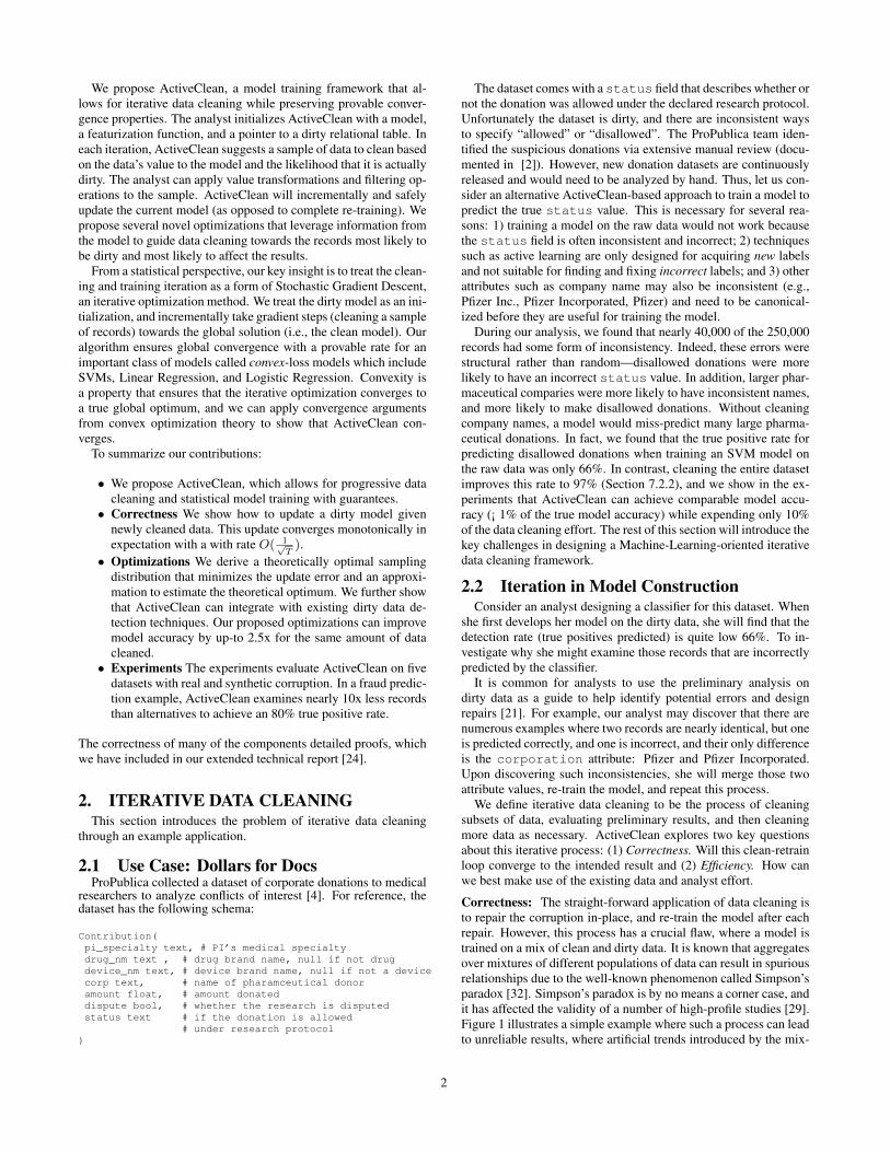
etry of the problem. Consider the problem in one dimension (i.e.,the parameter θ is a scalar value), so then the goal is to find theminimum point (θ) of a curve l(θ). The consequence of dirty datais that the wrong loss function is optimized. Figure 3A illustratesthe consequence of the optimization. The red dotted line shows theloss function on the dirty data. Optimizing the loss function findsθ(d) at the minimum point (red star). However, the true loss func-tion (w.r.t to the clean data) is in blue, thus the optimal value on thedirty data is in fact a suboptimal point on clean curve (red circle).

In the figure, the optimal clean model θ(c) is visualized as a yel-low star. The first question is which direction to update θ(d) (i.e.,left or right). For this class of models, given a suboptimal point,the direction to the global optimum is the gradient of the loss func-tion. The gradient is a p-dimensional vector function of the currentmodel θ(d) and the clean data. Therefore, ActiveClean needs toupdate θ(d) some distance γ (Figure 3B):

θnew ← θ(d) − γ · ∇φ(θ(d))

At the optimal point, the magnitude of the gradient will be zero.So intuitively, this approach iteratively moves the model downhill

4

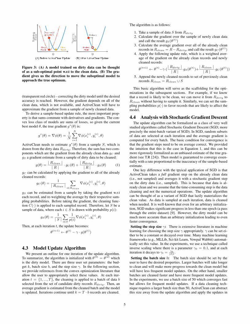
Figure 3: (A) A model trained on dirty data can be thoughtof as a sub-optimal point w.r.t to the clean data. (B) The gra-dient gives us the direction to move the suboptimal model toapproach the true optimum.

(transparent red circle) – correcting the dirty model until the desiredaccuracy is reached. However, the gradient depends on all of theclean data, which is not available, and ActiveClean will have toapproximate the gradient from a sample of newly cleaned data.

To derive a sample-based update rule, the most important prop-erty is that sums commute with derivatives and gradients. The con-vex loss class of models are sums of losses, so given the currentbest model θ, the true gradient g∗(θ) is:

g∗(θ) = ∇φ(θ) =1

N

N∑i=1

∇φ(x(c)i , y

(c)i , θ)

ActiveClean needs to estimate g∗(θ) from a sample S, which isdrawn from the dirty dataRdirty . Therefore, the sum has two com-ponents which are the gradient from the already clean data gC andgS a gradient estimate from a sample of dirty data to be cleaned:

g(θ) =| Rclean || R | · gC(θ) +

| Rdirty || R | · gS(θ) (1)

gC can be calculated by applying the gradient to all of the alreadycleaned records:

gC(θ) =1

| Rclean |∑

i∈Rclean

∇φ(x(c)i , y

(c)i , θ)

gS can be estimated from a sample by taking the gradient w.r.teach record, and re-weighting the average by their respective sam-pling probabilities. Before taking the gradient, the cleaning func-tion C(·) is applied to each sampled record. Therefore, let S be asample of data, where each i ∈ S is drawn with probability p(i):

gS(θ) =1

| S |∑i∈S

1

p(i)∇φ(x

(c)i , y

(c)i , θ)

Then, at each iteration t, the update becomes:

θ(t+1) ← θ(t) − γ · g(θ(t))

4.3 Model Update AlgorithmWe present an outline for one iteration of the update algorithm.

To summarize, the algorithm is initialized with θ(0) = θ(d) whichis the dirty model. There are three user set parameters: the bud-get k, batch size b, and the step size γ. In the following section,we provide references from the convex optimization literature thatallow the user to appropriately select these values. At each iter-ation t = {1, ..., T}, the cleaning is applied to a batch of data bselected from the set of candidate dirty records Rdirty . Then, anaverage gradient is estimated from the cleaned batch and the modelis updated. Iterations continue until k = T · b records are cleaned.

The algorithm is as follows:

1. Take a sample of data S from Rdirty2. Calculate the gradient over the sample of newly clean data

and call the result gS(θ(t))3. Calculate the average gradient over all of the already clean

records inRclean = R−Rdirty , and call the result gC(θ(t))4. Apply the following update rule, which is a weighted aver-

age of the gradient on the already clean records and newlycleaned records:

θ(t+1) ← θ(t)−γ·( | Rdirty || R | ·gS(θ(t))+| Rclean || R | ·gC(θ(t)))

5. Append the newly cleaned records to set of previously cleanrecords Rclean = Rclean ∪ S

This basic algorithm will serve as the scaffolding for the opti-mizations in the subsequent sections. For example, if we knowthat a record is likely to be clean, we can move it from Rdirty toRclean without having to sample it. Similarly, we can set the sam-pling probabilities p(·) to favor records that are likely to affect themodel.

4.4 Analysis with Stochastic Gradient DescentThe update algorithm can be formalized as a class of very well

studied algorithms called Stochastic Gradient Descent (SGD; moreprecisely the mini-batch variant of SGD). In SGD, random subsetsof data are selected at each iteration and the average gradient iscomputed for every batch. The basic condition for convergence isthat the gradient steps need to be on average correct. We providedthe intuition that this is the case in Equation 1, and this can bemore rigorously formalized as an unbiased estimate of the true gra-dient (see T.R [24]). Then model is guaranteed to converge essen-tially with a rate proportional to the inaccuracy of the sample-basedestimate.

One key difference with the tpyical application of SGD is thatActiveClean takes a full gradient step on the already clean data(i.e., not sampled) and averages it with a stochastic gradient stepon the dirty data (i.e., sampled). This is because that data is al-ready clean and we assume that the time-consuming step is the datacleaning and not the numerical operations. The update algorithmcan be thought of as a variant of SGD that lazily materializes theclean value. As data is sampled at each iteration, data is cleanedwhen needed. It is well-known that even for an arbitrary initializa-tion, SGD makes significant progress in less than one epoch (a passthrough the entire dataset) [9]. However, the dirty model can bemuch more accurate than an arbitrary initialization leading to evenfaster convergence.Setting the step size γ: There is extensive literature in machine

learning for choosing the step size γ appropriately. γ can be set ei-ther to be a constant or decayed over time. Many machine learningframeworks (e.g., MLLib, Sci-kit Learn, Vowpal Wabbit) automat-ically set this value. In the experiments, we use a technique calledinverse scaling where there is a parameter γ0 = 0.1, and at eachiteration it decays to γt = γ0

|S|t .

Setting the batch size b: The batch size should be set by theuser to have the desired properties. Larger batches will take longerto clean and will make more progress towards the clean model butwill have less frequent model updates. On the other hand, smallerbatches are cleaned faster and have more frequent model updates.In the experiments, we use a batch size of 50 which converges fastbut allows for frequent model updates. If a data cleaning tech-nique requires a larger batch size than 50, ActiveClean can abstractthis size away from the update algorithm and apply the updates in

5

smaller batches. For example, the batch size set by the user mightbe b = 1000, but the model updates after every 50 records arecleaned. We can disassociate the batching requirements of SGDand the batching requirements of the data cleaning technique.Convergence Conditions and Properties The convergence ratesof SGD are also well analyzed [8,11,37]. The analysis gives abound on the error of intermediate models and the expected num-ber of steps before achieving a model within a certain error. Fora general convex loss, a batch size b, and T iterations, the conver-gence rate is bounded by O( σ2

√bT

). σ2 is a measure of how wellthe sample gradient estimates the gradient over the entire dataset,and√T shows that each iteration has diminishing returns. σ2 is

the variance in the estimate of the gradient at each iteration:σ2 = E(‖g − g∗‖2)

where g∗ is the gradient computed over the full data if it werefully cleaned. This property of SGD allows us to bound the modelerror with a monotonically decreasing function of the number ofrecords cleaned, thus satisfying the reliability condition in the prob-lem statement.

Gradient descent techniques also can be applied to non-convexlosses and they are widely used in graphical model inference anddeep learning. In this case, however, instead of converging to aglobal optimum, they converge to a locally optimal value that de-pendends on the initialization. In the non-convex setting, Active-Clean will converge to the closest locally optimal value to the dirtymodel which is how we initialize ActiveClean. Because of this, itis harder to reason about the objective quality of the results and todefine accuracy. Different initializations may lead to different localoptima, and thus, introduce a complex dependence on the initial-ization with the dirty model.

EXAMPLE 2. Recall that the analyst has a dirty SVM model onthe dirty data θ(d). She decides that she has a budget of cleaning100 records, and decides to clean the 100 records in batches of 10(set based on how fast she can clean the data, and how often shewants to see an updated result). All of the data is initially treatedas dirty with Rdirty = R and Rclean = ∅. The gradient of a basicSVM is given by the following function:

∇φ(x, y, θ) =

{−y · x if yx · θ < 1

0 if yx · θ ≥ 1

For each iteration t, a sample of 10 records S is drawn fromRdirty . ActiveClean then applies the cleaning function to the sam-ple. Using these values, ActiveClean estimates the gradient on thenewly cleaned data:

1

10

∑i∈S

1

p(i)∇φ(x

(c)i , y

(c)i , θ)

ActiveClean also applies the gradient to the already clean data (ini-tially non-existent):

1

| Rclean |∑

i∈Rclean

∇φ(x(c)i , y

(c)i , θ)

Then, it calculates the update rule:

θ(t+1) ← θ(t) − γ · ( | Rdirty || R | · gS(θ(t)) +| Rclean || R | · gC(θ(t)))

Finally,Rdirty ← Rdirty−S,Rclean ← Rclean+S, and continueto the next iteration.

5. DIRTY DATA DETECTIONIf corrupted records are relatively rare, sampling might be very

inefficient. The analyst may have to sample many batches of databefore finding a corrupted record. In this section, we describe howwe can couple ActiveClean with prior knowledge about which dataare likely to be dirty. In the data cleaning literature, error detectionand error repair are treated as two distinct problems [10,14,30]. Er-ror detection is often considered to be substantially easier than er-ror repair since one can declare a set of integrity rules on a database(e.g., an attribute must not be NULL), and select rows that violatethose rules. On the other hand, repair is harder and often requireshuman involvement (e.g., imputing a value for the NULL attribute).

5.1 Detection ProblemFirst, we describe the required properties of the dirty data de-

tector. The detector returns two important aspects of a record: (1)whether the record is dirty, and (2) if it is dirty, on which attributesthere are errors. The sampler can use (1) to select a subset of dirtyrecords to sample at each batch and the estimator can use (2) toestimate the value of data cleaning based on other records with thesame corruption.

DEFINITION 1 (DETECTOR). Let r be a record in R. A de-tector is a function that returns a Boolean of whether the record isdirty and a set of attributes er that are dirty.

D(r) = ({0, 1}, er)

From the set of attributes that are dirty, we can find the corre-sponding features that are dirty fr and labels that are dirty lr sincewe assume a one-to-one mapping between records and trainingexamples. We will consider two types of detectors: exact rule-based detectors that detect integrity constraint or functional de-pendency violations, and approximate adaptive detectors that learnwhich data are likely to be dirty.

5.2 Rule-Based DetectorData quality rules are widely studied as a technique for detect-

ing data errors. In most rule-based frameworks, an analyst declaresa set of rules Σ and checks whether a relation R satisfies thoserules. The rules rules can be declared in advance before applyingActiveClean, or constructed from the first batch of sampled data.ActiveClean is compatible with many commonly used classes ofrules for error detection including integrity constraints (ICs), con-ditional functional dependencies (CFDs), and matching dependen-cies (MDs). The only requirement on the rules is that there is analgorithm to enumerate the set of records that violate at least onerule.

LetRviol andRsat be the subset of records inRditry that violateat least one rule and satisfy all rules respectively. The rule-baseddetector modifies the update workflow in the following way:

1. Rclean = Rclean ∪Rsat

2. Rdirty = Rviol

3. Apply the algorithm in Section 4.3.

EXAMPLE 3 (RULE-BASED DETECTION). An example of arule on the running example dataset is that the status of a con-tribution can be only “allowed” or “disallowed”. Any other valuefor status is considered violation.

6

5.3 Adaptive DetectionRule-based detection is not possible in all cases, especially in

cases where the analyst selectively modifies data. This is why wepropose an alternative called the adaptive detector. Essentially, wereduce the problem to training a classifier on previously cleaneddata. Note that this “learning” is distinct from the “learning” in theuser-specified statistical model. One challenge is that the detectorneeds to describe how the data is dirty. The detector achieves thisby categorizing the corruption into u classes, and using a multi-class classifier. These classes are corruption categories that do notnecessarily align with features, but every record is classified withat most one category.

When using adaptive detection, the repair step has to clean thedata and report to which of the u classes the corrupted record be-longs. When an example (x, y) is cleaned, the repair step labelsit with one of the clean, 1, 2, ..., u. It is possible that u increaseseach iteration as more types of dirtiness are discovered. In manyreal world datasets, data errors have locality, where similar recordstend to be similarly corrupted. There are usually a small numberof error classes even if a large number of records are corrupted.This problem can be addressed by any classifier, and we use anall-versus-one Logistic Regression in our experiments.

The adaptive detector modifies the update workflow in the fol-lowing way:

1. Let Rclean be the previously cleaned data, and let Uclean bea set of labels for each record indicating the error class and ifthey are dirty or “not dirty”.

2. Train a classifier to predict the label Train(Rclean, Uclean)

3. Apply the classifier to the dirty data Predict(Rdirty)

4. For all records predicted to be clean, remove from Rdirtyand append to Rclean.

5. Apply the algorithm in Section 4.3.

The precision and recall of this classifier should be tuned to favorclassifying a record as dirty to avoid falsely moving a dirty recordintoRclean. In our experiments, we set this value to 0.90 probabil-ity of the “clean” class.

6. SELECTING RECORDS TO CLEANThe algorithm proposed in Section 4.3 will convege for any sam-

pling distribution where p(·) > 0 for all records, albeit differentdistributions will have different convergence rates. The samplingalgorithm is designed to include records in each batch that are mostvaluable to the analyst’s model with a higher probability.

6.1 Optimal Sampling ProblemRecall that the convergence rate of an SGD algorithm is bounded

by σ2 which is the variance of the gradient. Intuitively, the variancemeasures how accurately the gradient is estimated from a uniformsample. Other sampling distributions, while preserving the sameexpected value, may have a lower variance. Thus, the optimal sam-pling problem is defined as a search over sampling distributions tofind the minimum variance sampling distribution.

DEFINITION 2 (OPTIMAL SAMPLING PROBLEM). Given a setof candidate dirty data Rdirty , ∀r ∈ Rdirty find sampling proba-bilities p(r) such that over all samples S of size k it minimizes thevariance:

arg minp

E(‖gS − g∗‖2)

It can be shown [37] that the optimal distribution over records inRdirty is proportional to: pi ∝ ‖∇φ(x

(c)i , y

(c)i , θ(t))‖ Intuitively,

this sampling distribution prioritizes records with higher gradients,i.e., make a larger impact during optimization. The challenge is thatthis particular optimal distribution depends on knowing the cleanvalue of a records, which is a chicken-and-egg problem: the opti-mal sampling distribution requires knowing (x

(c)i , y

(c)i ); however,

we are sampling the values so that they can be cleaned.One natural solution is to calculate this gradient with respect to

the dirty values–implicitly assuming that the corruption is not thatsevere:

pi ∝ ‖∇φ(x(d)i , y

(d)i , θ(t))‖

This solution is highly related to the Expected Gradient Lengthheuristic that has been proposed before in Active Learning [31].However, there is additional structure to the data cleaning problem.As the analyst cleans more data, we can build a model for howcleaned data relates to dirty data. By using the detector from theprevious section to estimate the impact of data cleaning, we showthat we can estimate the cleaned values. We find that this opti-mization can improve the convergence rate by a factor of 2 in somedatasets.

6.2 The EstimatorWe call this component, the estimator, which connects the de-

tector and the sampler. The goal of the estimator is to estimate∇φ(x

(c)i , y

(c)i , θ(t)) (the clean gradient) using∇φ(x

(d)i , y

(d)i , θ(t))

(the dirty gradient) andD(r) (the detection results). As a strawmanapproach, one could use all of the previously cleaned data (tuplesof dirty and clean records), and use another learning algorithm torelate the two. The main challenges with this approach are: (1)the problem of scarcity where errors may affect a small number ofrecords and a small number of attributes and (2) the problem ofmodeling where if we have an accurate parametric model relatingclean to dirty data then why clean the data in the first place. Toaddress these challenges, we propose a light-weight estimator usesa linear approximation of the gradient and only relies on the av-erage change in each feature value. Empirically, we find that thisestimator provides more accurate early estimates and is easier totune than the strawman approach until a large amount of data arecleaned (Section 7.4.6).

6.3 Linearization AlgorithmThe basic idea is for every feature i to maintain an average change

δi before and after cleaning–estimated from the previously cleaneddata. This avoids having to design a complex internal model to re-late the dirty and clean data, and is based on just estimating samplemeans. This would work if the gradient was linear in the features,and we could write this estimate as:∇φ(x

(c)i , y

(c)i , θ(t)) ≈ ∇φ(x

(d)i , y

(d)i , θ(t)) +A · [δ1, ..., δp]ᵀ

The problem is that the gradient ∇φ(·) can be a very non-linearfunction of the features that couple features together. For example,even in the simple case of linear regression, the gradient is a non-linear function in x:

∇φ(x, y, θ) = (θTx− y)x

It is not possible to isolate the effect of a change of one featureon the gradient. Even if one of the features is corrupted, all of thegradient components can be incorrect.

The way that we address this problem is to linearize the gradi-ent, where the matrix A is found by computing a first-order Taylor

7

Series expansion of the gradient. If d is the dirty value and c isthe clean value, the Taylor series approximation for a function f isgiven as follows:

f(c) = f(d) + f ′(d) · (d− c) + ...

In our case, the function f is the gradient ∇φ, and the linear termf ′(d) · (d− c) is a linear function in each feature and label:

∇φ(x(c)i , y

(c)i , θ(t)) ≈ ∇φ(x

(d)i , y

(d)i , θ(t))

+∂

∂X∇φ(x

(d)i , y

(d)i , θ(t)) · (x(d) − x(c))

+∂

∂Yφ(x

(d)i , y

(d)i , θ(t)) · (y(d) − y(c))

This can be simplified with two model-dependent matrices Mx

(relating feature changes to the gradient) and My (relating labelchanges to the gradient) 1:

≈ φ(x(d)i , y

(d)i , θ(t)) +Mx ·∆x+My ·∆y

where ∆x = [δ1, ..., δp]ᵀ is the average change in each feature and

∆y = [δ1, ..., δl]ᵀ is the average change in each label. It follows

that the resulting sampling distribution is:

p(r) ∝ ‖∇φ(x(d)i , y

(d)i , θ(t)) +Mx ·∆x +My ·∆y‖

7. EXPERIMENTSWe start by presenting two end-to-end scenarios based on a dataset

of movies from IMDB and a dataset of medical donations fromProPublica. Then, we evaluate each of the components of Ac-tiveClean on standard Machine Learning benchmarks (Tax RecordClassification, EEG anomaly detection) with synthetic errors.

7.1 SetupWe compare ActiveClean to alternative solutions along two pri-

mary axes: the sampling procedure to pick the next set of recordsto clean, and the model update procedure to incorporate the cleanedsample. All of the compared approaches clean the same amount ofdata, and we evaluate the accuracy of the approaches as a functionof the amount of data examined; defined as the number of evalua-tions of the user-specified C() (cleaner) on a record whether or notthe record is actually dirty.Naive-Mix (NM): In each iteration, Naive-Mix draws a randomsample, merges the cleaned sample back into the dataset, and re-trains over the entire dataset.Naive-Sampling (NS): In contrast to Naive-Mix, Naive-Samplingonly re-trains over the set of records that have been cleaned so far.Active Learning (AL): The samples are picked using Active Learn-ing (more precisely, Uncertainty Sampling [31]), and the model isre-trained over the set of records cleaned so far.Oracle (O): Oracle has complete access to the ground truth, andin each iteration, selects samples that maximize the expected con-vergence rate. It uses ActiveClean’s model update procedure.Metrics: We evaluate these approaches on two metrics: modelerror, which is the distance between the trained model and truemodel if all data were cleaned ‖θ − θ(c)‖, and test error, which isthe prediction accuracy of the model on a held out set of clean data.

7.2 Real ScenariosWe now describe two data analyst classification scenarios based

on popular industry use cases reported in the Apache Spark user

1A number of example linearizations are listed in [24]

survey [1] — these experiments are run with real data and real cor-ruption. The first is a content tagging problem to categorize moviesfrom plot descriptions; the second is a fraud detection problem todetermine whether a medical donation is suspicious. Both of thedatasets are plagued by systematic errors that affect the classifi-cation accuracy by 10 − 35%. One indication of the systematicnature of the data error is that errors disproportionately affect oneclass rather than another. We simulate the analyst’s cleaning proce-dure by looking up the cleaned value in the dataset that we cleanedbeforehand. See [24] for constraints, errors, and cleaning method-ology, as well as an additional regression scenario.

7.2.1 Movie PredictionThe first scenario uses two published datasets about movies, from

IMDB 2 and Yahoo 3. Each movie has a title, a short 1-2 paragraphplot description, and a list of categories, and the goal is to traina model to predict whether a movie is a “Horror” or “Comedy”from the description and title. The text data was featurized using aTFIDF model.

The IMDB dataset has 486,298 movies and is very dirty. Thecategory list of many movies has redundant and possibly conflict-ing tags (e.g., “Kids” and “Horror” for the same movie). Also, theplot and title text may have errors from the scraping procedure (e.g.,“brCuin, the”). This dataset also shows experimental evidence forsystematic bias. Horror movies were more likely to be erroneouslytagged, and consequently, a classifier trained on the dirty data fa-vored “Comedy” predictions. In contrast, the smaller Yahoo dataset(106,959 movies) is much cleaner, and nearly all of the movies arefound in the IMDB dataset.

To clean the category lists, this smaller dataset to cross-referencingrecords when possible and import categories from Yahoo. This wasdone using a simple entity resolution to match movie titles betweenthe two dataset. When there was a sufficiently close textual match(in terms of title string similarity), we imported the Yahoo dataset’scategory list to the IMDB dataset. For the movies that did notmatch, we appended the records to the IMDB dataset. Finally, wefiltered the dataset for movies whose category lists included “Hor-ror” or “Comedy”. To clean the parsing errors, we identify commonparsing artifacts in each sampled batch and write a script to fix allrecords with that problem (e.g., remove all instances of “C”).

Figure 4a plots the model error and test error versus the numberof records examined by each algorithm. For very small batches ofdata (e.g., 50 out of 400,000), some of the techniques are actuallyless accurate than the dirty model. This is because the error due tothe particular initial sampled batch of dominates, and we find thatdifferences between the techniques are not statistically significantin that regime. However, as more data is cleaned, we see a clearseperation between the techniques The purple bottom curve is theOracle approach, and we find that out of the practical approachesActiveClean reduces the model error the fastest, and is the onlymethod that converges to the Oracle performance. Figure 4b di-rectly shows how ActiveClean rapidly reduces the test error — af-ter 2000 records, ActiveClean’s test error is within 0.02 of the fullycleaned model. ActiveClean provides superior convergence for twomain reasons. First, the update algorithm can incorporate both theraw data as well as the smaller set of cleaned records. This makesActiveClean less sensitive to sampling error. Next, ActiveCleanalso selects records that are more likely to by dirty (Section 5) andwill will most improve the model (Section 6). This is illustratedin ActiveClean’s faster convergence curve in the first 2000 cleanedrecords.2ftp://ftp.fu-berlin.de/pub/misc/movies/database/

3http://webscope.sandbox.yahoo.com/catalog.php?datatype=r

8

Figure 4: (a) We plot the relative model error as a function of the number of records cleaned for each of the alternatives on the IMDBcontent tagging task. ActiveClean results in the fastest convergence. (b) Faster convergence translates into improved test accuracy.On a holdout set of 20%, ActiveClean is more accurate than the alternatives. (c) We evaluate ActiveClean on the Dollars For Docsfraud detection task and find similar results, where ActiveClean converges faster than the alternatives. (d) ActiveClean improves thefalse negative rate (detection error) of the classifier resulting in an improved fraud detector.

0

5

10

15

20

0 2000 4000 6000 8000 10000

Mod

el E

rror

%

# Images Cleaned

MNIST Block Removal 5x5

0 2 4 6 8

10 12

0 1000 2000 3000 4000 5000

Mod

el E

ror

%

# Images Cleaned

MNIST Fuzzy

Figure 5: In an image processing pipeline on the MNISTdataset with simulated errors, ActiveClean outperforms ActiveLearning and Naive-Sample.

7.2.2 Dollars For Docs (DfD)The second scenario explores ProPublica’s Dollars for Docs dataset

described in Section 2.1. We featurize the 5 text attributes using abag-of-words representation, and our goal is to predict the statusof medical donations using an SVM (“allowed” or “disallowed”).Figure 4c plots the model error as a function of the number ofrecords examined for each of the techniques. As in the IMDBdataset, we find that ActiveClean converges faster than Naive-Mix,Naive-Sampling, and Active Learning. In fact, ActiveClean canachieve comparable model accuracy (¡ 1% of the true model accu-racy) while expending a fraction of the data cleaning effort (10%of the records cleaned).

In terms of test error, Figure 4d reports the detection error orfalse negative % (percentage of disallowed research contributionsthat the model misses) on a held-out evaluation set. This mea-sures the real-world utility of the classifier learned with Active-Clean. The dirty and fully cleaned models have respectively a 34%and 3% detection error. Due to the systematic bias in the data er-rors (explained in Section 2.1), ActiveClean is able to identify thedirty records and reduce the detection error to 8% after examining10,000 records.

Overall, we found that systematic errors are indeed present inreal-world datasets, and that ActiveClean can effectively identifyand exploit this bias to more quickly converge to the true cleanmodel as compared to the naive or active learning approaches. Infact, we found that the commonly used retraining approach (Naive-Mix) was almost completely ineffective as compared to other modelupdate techniques.

7.3 Simulated Machine Learning PipelineThis experiment is representative of modern machine learning

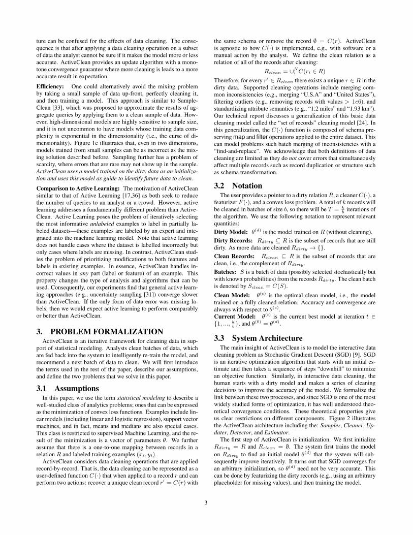
pipelines such as AMPLab’s Keystone ML [3] and Google’s Ten-sor Flow [5]. The task is to classify 60,000 images of handwrittendigits from the MNIST dataset into 10 categories with a one-to-all multiclass SVM classifier 4. In contrast to the prior scenarios,which directly extracted feature vectors from the raw dataset, im-age feature extraction involves a pipeline of transformation stepsincluding edge detection, projection, and raw image patch extrac-tion [3,5]. The cleaning function C() involves replacing a poten-tially corrupted image with a non-corrupted version. We find thatpipelines tend to propagate small amounts of corruption, and infact, and even randomly generated errors can morph into system-atic biases.

There are two types of simulated corruptions that mimic standardcorruptions in image processing (occlusion and low-resolution):5x5 Removal deletes a random 5x5 pixel block by setting thepixel values to 0, and Fuzzy blurs the entire image using a 4x4moving average patch. We apply these corruptions to a random 5%of the images.

Figure 5 shows that ActiveClean makes more progress towardsthe clean model with a smaller number of examples cleaned. Toachieve a 2% error for 5x5 Removal, ActiveClean can inspect 2200fewer images than Active Learning and 2750 fewer images thanNaive-Sampling. For the fuzzy images, both Active Learning andActiveClean reach 2% error after examining < 100 images, whileNaive-Sampling requires 1750. Even though these corruptions aregenerated independently of the data, the 5x5 Removal propa-gates through the pipeline as a systematic error. The image fea-tures are constructed with edge detectors, which are highly sen-sitive to this type of corruption. Digits that naturally have feweredges than others are disproportionately affected since the removalprocess adds spurious edges. On the other hand, the Fuzzy cor-ruption propagates through the pipeline are similar to random errors(as opposed to systematic).

7.4 Simulated Error ScenariosIn the next set of experiments, we use standard Machine Learn-

ing benchmark datasets and corrupt them with varying levels ofsystematic noise. We use this to evaluate ActiveClean while isolat-ing certain variables. The two datasets that we used were:

4http://ufldl.stanford.edu/wiki/index.php/Using_the_

MNIST_Dataset

9

0% 10% 20% 30% 40% 50% 60% 70% 80% 90%

100%

EEG Adult

Test

Acc

urac

y (a) Randomly Corrupted Data

0% 10% 20% 30% 40% 50% 60% 70% 80% 90%

100%

EEG Adult

Test

Acc

urac

y

(b) Systematically Corrupted Data

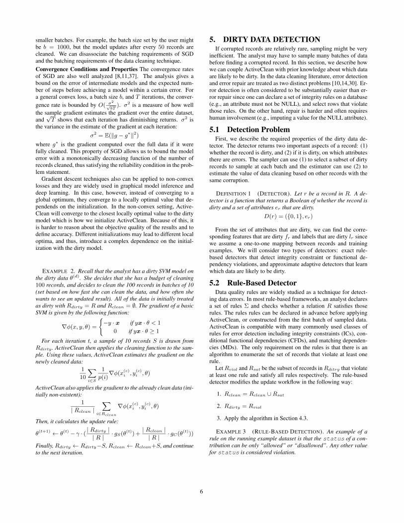
Figure 6: (a) Robust techniques and discarding data workwhen corrupted data are random and look atypical. (b) Datacleaning can provide reliable performance in both the system-atically corrupted setting and randomly corrupted setting.

Income Classification (Adult): In this dataset of 45,552 records,the task is to predict the income bracket (binary) from 12 numericaland categorical covariates with an SVM classifier.Seizure Classification (EEG): In this dataset, the task is to predictthe onset of a seizure (binary) from 15 numerical covariates with athresholded Linear Regression. There are 14980 data points in thisdataset. This classification task is inherently hard with an accuracyon the completely clean data of only 65%.

7.4.1 Data Cleaning v.s. Robust StatisticsMachine Learning has broadly studied a number of robust meth-

ods to deal with some types of outliers. In particular, this field stud-ies random high-magnitude outliers and techniques to make statisti-cal model training agnostic to their presence. Feng et al. proposeda variant of logistic regression that is robust to outliers [16]. Wechose this algorithm because it is a robust extension of the convexregularized loss model, leading to a better apples-to-apples com-parison between the techniques. Our goal is to understand whichtypes of data corruption are amenable to data cleaning and whichare better suited for robust statistical techniques. The experimentcompares four schemes: (1) full data cleaning, (2) baseline of nocleaning, (3) discarding the dirty data, and (4) robust logistic re-gression. We corrupted 5% of the training examples in each datasetin two different ways:

Random Corruption: Simulated high-magnitude random out-liers. 5% of the examples are selected at random and a randomfeature is replaced with 3 times the highest feature value.

Systematic Corruption: Simulated innocuous looking (but stillincorrect) systematic corruption. The model is trained on the cleandata, and the three most important features (highest weighted) areidentified. The examples are sorted by each of these features andthe top examples are corrupted with the mean value for that feature(5% corruption in all).

Figure 6 shows the test accuracy for models trained on both typesof data with the different techniques. The robust method performswell on the random high-magnitude outliers with only a 2.0% re-duction in clean test accuracy for EEG and 2.5% reduction forAdult. In the random setting, discarding dirty data also performsrelatively well. However, the robust method falters on the system-atic corruption with a 9.1% reduction in clean test accuracy forEEG and 10.5% reduction for Adult. Data cleaning is the most re-liable option across datasets and corruption types. The problem isthat without cleaning, there is no way to know if the corruption israndom or systematic and when to trust a robust method. While

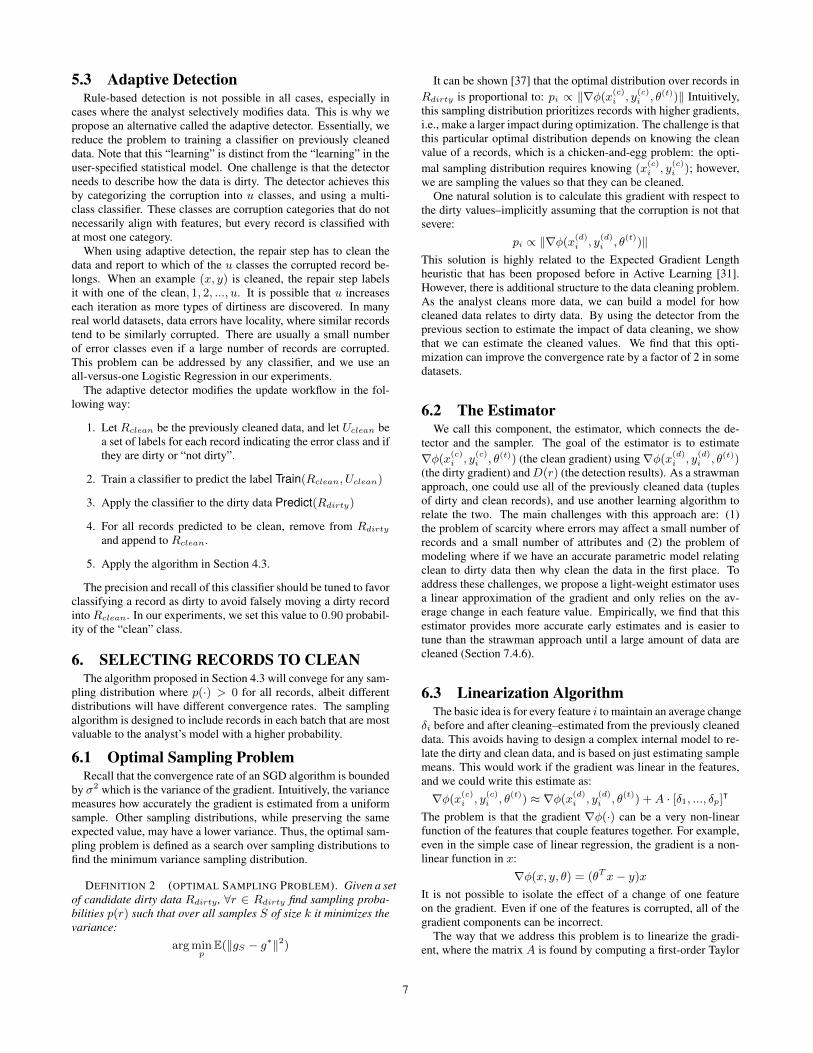
Figure 7: -D denotes no detection, and -D-I denotes no detec-tion and no importance sampling. Both optimizations signif-icantly help ActiveClean outperform Naive-Sampling and Ac-tive Learning.

data cleaning requires more effort, it provides benefits in both set-tings. The remaining experiments, unless otherwise noted, use sys-tematic corruption.

7.4.2 Source of ImprovementsThis experiment compares the performance of ActiveClean with

and without various optimizations for 500 records examined. Ac-tiveClean without detection is denoted as (AC-D) (that is at eachiteration we sample from the entire dirty data), and ActiveCleanwithout detection and our prioritized sampling is denoted as (AC-D-I). Figure 7 plots the relative error of the alternatives and Ac-tiveClean with and without the optimizations. Without detection(AC-D), ActiveClean is still more accurate than Active Learning.Removing the sampling, ActiveClean is slightly worse than Ac-tive Learning on the Adult dataset but is comparable on the EEGdataset. The advantage of ActiveClean is that it is a composableframework supporting different instantiations of the detection andprioritization modules while still preserving convergence guaran-tees. With these optimizations, ActiveClean is consistently moreefficient than Active Learning.

7.4.3 Mixing Dirty and Clean DataNaive-Mix is an unreliable methodology lacking the same guar-

antees as Active Learning or Naive-Sampling even in the simplestof cases. We also saw that it is significantly less efficient than Ac-tiveClean, Naive-Sampling, and Active Learning on the real datasets.For thoroughness, these experiments include the model error as afunction of records examined in comparison to ActiveClean. Wealso evaluate this approach with our detection component. Naive-Mix+D randomly samples data using the dirty data detector, appliesthe user-specified cleaning, and writes-back the cleaned data.

Figure 8 plots the same curves as the previous experiment com-paring ActiveClean, Active Learning, and two mixed data algo-rithms. Intuitively, Naive-Mix makes less progress with each up-date. Consider the case where 10% of the dataset is corrupted anda small sample of data 1%. ActiveClean and Naive-Sampling ex-trapolate from the cleaned sample (ActiveClean extrapolates a gra-dient) while Naive-Mix considers the entire dirty data which mightbe much larger.

7.4.4 Corruption RateThis experiment explores the tradeoff between Naive-Sampling

and ActiveClean. Figure 9 varies the systematic corruption rate andplots the number of records examined to achieve 1% relative errorfor Naive-Sampling and ActiveClean. Naive-Sampling does notuse the dirty data and thus its error is essentially governed by thethe sample size and not the magnitude or prevalence of corruption.

10

0 1 2 3 4 5

0 1000 2000 3000 4000 5000

Mod

el E

rror

%

# Records Cleaned

(a) Adult

0

5

10

15

20

0 1000 2000 3000 4000 5000

Mod

el E

rror

%

# Records Cleaned

(b) EEG

Figure 8: The relative model error as a function of the num-ber of examples cleaned. ActiveClean converges with a smallersample size to the true result in comparison to partial cleaning(NM, NM+D).

0 20 40 60 80

0 2000 4000 6000

Err

or R

ate

# Examined to 1% Error

(a) Adult

AC NS 0

20 40 60 80

0 2000 4000 6000

Err

or R

ate

# Examined to 1% Error

(b) EEG

AC NS

Figure 9: ActiveClean outperforms Naive until the corruptionis so severe that the dirty model is initialized very far away fromthe clean model. The error of Naive-Sampling does not dependon the corruption rate so it is a vertical line.

Naive-Sampling outperforms ActiveClean only when corruptionsare very severe (45% in Adult and nearly 60% in EEG). When theinitialization with the dirty model is inaccurate, ActiveClean doesnot perform as well.

7.4.5 Dirty Data DetectionAdaptive detection depends on predicting which records are dirty;

and this is again related to the systematic nature of data error. Forexample, random corruption not correlated with any other data fea-tures may be hard to learn. As corruption becomes more random,the classifier becomes increasingly erroneous. This experiment ex-plores making our generated systematic corruption incrementallymore random. Instead of selecting the highest valued records forthe most valuable features, we corrupt random records with proba-bility p. We compare these results to AC-D where we do not have adetector at all (for a fixed number of 1000 records examined). Fig-ure 10a plots the relative error reduction using a classifier. Whenthe corruption is about 50% random then there is a break even pointwhere no detection is better. The classifier is imperfect and misclas-sifies some data points incorrectly as cleaned.

7.4.6 Impact EstimationThis experiment compares estimation techniques: (1) “linear re-

gression” trains a linear regression model that predicts the cleangradient as a function of the dirty gradient, (2) “average gradient”which does not use the detection to inform how to apply the esti-mate, (3) “average feature change” uses detection but no lineariza-tion, and (4) the Taylor series linear approximation. Figure 10bmeasures how accurately each estimation technique estimates thegradient as a function of the number of examined records on theEEG dataset. Estimation error is measured using the relative L2error with the true gradient. The Taylor series approximation pro-posed gives more accurate for small cleaning sizes.

0 0.5

1 1.5

2 2.5

3

0 0.2 0.4 0.6 0.8 1

Err

or R

educ

tion

(a) Error Randomness

EEG

Adult

Baseline

0%

5%

10%

15%

100 500 1000 5000

Est

imat

ion

Err

or

(b) Records Cleaned

Regression Avg Gradient Avg Change Taylor

Figure 10: (a) Data corruptions that are less random are easierto classify, and lead to more significant reductions in relativemodel error. (b) The Taylor series approximation gives moreaccurate estimates when the amount of cleaned data is small.

8. RELATED WORKData Cleaning: There are a number of other works that use ma-chine learning to improve the efficiency and/or reliability of datacleaning [17,35,36]. For example, Yakout et al. train a model thatevaluates the likelihood of a proposed replacement value [35]. An-other application of machine learning is value imputation, wherea missing value is predicted based on those records without miss-ing values. Machine learning is also increasingly applied to makeautomated repairs more reliable with human validation [36]. Hu-man input is often expensive and impractical to apply to entire largedatasets. Machine learning can extrapolate rules from a small setof examples cleaned by a human (or humans) to uncleaned data[17,36]. This approach can be coupled with active learning [25] tolearn an accurate model with the fewest possible number of exam-ples. While, in spirit, ActiveClean is similar to these approaches,it addresses a very different problem of data cleaning before user-specified modeling.

SampleClean [33] applies data cleaning to a sample of data, andestimates the results of aggregate queries. Sampling has also beenapplied to estimate the number of duplicates in a relation [19]. Sim-ilarly, Bergman et al. explore the problem of query-oriented datacleaning [7], where given a query, they clean data relevant to thatquery. Deshpande et al. studied data acquisition in sensor net-works [12]. They explored value of information based prioritiza-tion of data acquisition for estimating aggregate queries of sensorreadings. Similarly, Jeffery et al. [20] explored similar prioritiza-tion based on value of information. Existing work does not explorecleaning driven by the downstream machine learning “queries” stud-ied in this work.

Stochastic Optimization and Active Learning: Zhao and Tongrecently proposed using importance sampling in conjunction withstochastic gradient descent [37]. This line of work builds on priorresults in linear algebra that show that some matrix columns aremore informative than others [13], and Active Learning which showsthat some labels are more informative that others [31]. ActiveLearning largely studies the problem of label acquisition [31], andrecently the links between Active Learning and Stochastic opti-mization have been studied [18].

Transfer Learning and Bias Mitigation: ActiveClean has a stronglink to a field called Transfer Learning and Domain Adaptation[27]. The basic idea of Transfer Learning is that suppose a modelis trained on a dataset D but tested on a dataset D′. Much of thecomplexity and contribution of ActiveClean comes from efficientlytuning such a process for expensive data cleaning applications –costs not studied in Transfer Learning. Other problems in bias mit-igation (e.g., Krishnan et al. [23]) have the same structure, system-atically corrupted data that is feeding into a model. In this work,

11

we try to generalize these principles given a general dirty dataset,convex model, and data cleaning procedure.

Secure Learning: ActiveClean is also related to work in adversar-ial learning [26], where the goal is to make models robust to adver-sarial data manipulation. This line of work has extensively stud-ied methodologies for making models private to external queriesand robust to malicious labels [34], but the data cleaning prob-lem explores more general corruptions than just malicious labels.One widely applied technique in this field is reject-on-negative im-pact, which essentially, discards data that reduces the loss function–which will not work when we do not have access to the true lossfunction (only the “dirty loss”).

9. CONCLUSIONThe growing popularity of predictive models in data analytics

adds additional challenges in managing dirty data. We propose Ac-tiveClean, a model training framework that allows for iterative datacleaning while preserving provable convergence properties. Wespecifically focus on problems that arise when data error is system-atic, i.e., correlated with the hypotheses of interest. The key insightof ActiveClean is that convex loss models (e.g., linear regressionand SVMs) can be simultaneously trained and cleaned. Active-Clean also includes numerous optimizations such as: using the in-formation from the model to inform data cleaning on samples, dirtydata detection to avoid sampling clean data, and batching updates.The experimental results are promising as they suggest that theseoptimizations can significantly reduce data cleaning costs when er-rors are sparse and cleaning budgets are small. Techniques such asActive Learning and SampleClean are not optimized for the sparselow-budget setting, and ActiveClean achieves models of high accu-racy for significantly less records cleaned.

This research is supported in part by DHS Award HSHQDC-16-3-00083, NSF CISE Expeditions Award CCF-1139158, DOE AwardSN10040 DE-SC0012463, an SFU Presidents Research Start-up Grant(NO. 877335), and DARPA XData Award FA8750-12-2-0331, and giftsfrom Amazon Web Services, Google, IBM, SAP, The Thomas and StaceySiebel Foundation, Apple Inc., Arimo, Blue Goji, Bosch, Cisco, Cray,Cloudera, Ericsson, Facebook, Fujitsu, HP, Huawei, Intel, Microsoft,Pivotal, Samsung, Schlumberger, Splunk, State Farm and VMware.

10. REFERENCES[1] Apache spark survey.

https://databricks.com/blog/2015/09/24/spark-survey-results-2015-are-now-available.html.

[2] Dollars for docs.https://projects.propublica.org/docdollars/.

[3] Keystone ml. http://keystone-ml.org/.[4] A pharma payment a day keeps docs’ finances okay.

https://www.propublica.org/article/a-pharma-payment-a-day-keeps-docs-finances-ok.

[5] Tensor flow. https://www.tensorflow.org/.[6] Y. Altowim, D. V. Kalashnikov, and S. Mehrotra. Progressive

approach to relational entity resolution. In VLDB, 2014.[7] M. Bergman, T. Milo, S. Novgorodov, and W. C. Tan. Query-oriented

data cleaning with oracles. In SIGMOD, 2015.[8] D. P. Bertsekas. Incremental gradient, subgradient, and proximal

methods for convex optimization: A survey. In CoRR, 2015.[9] L. Bottou. Stochastic gradient descent tricks. In Neural Networks:

Tricks of the Trade. 2012.[10] T. Dasu and T. Johnson. Exploratory Data Mining and Data

Cleaning. John Wiley & Sons, Inc., 2003.[11] O. Dekel, R. Gilad-Bachrach, O. Shamir, and L. Xiao. Optimal

distributed online prediction using mini-batches. In JMLR, 2012.

[12] A. Deshpande, C. Guestrin, S. Madden, J. M. Hellerstein, andW. Hong. Model-driven data acquisition in sensor networks. InVLDB, 2004.

[13] P. Drineas, M. Magdon-Ismail, M. W. Mahoney, and D. P. Woodruff.Fast approximation of matrix coherence and statistical leverage. InJMLR, 2012.

[14] W. Fan and F. Geerts. Foundations of Data Quality Management.Synthesis Lectures on Data Management. 2012.

[15] U. Fayyad, G. Piatetsky-Shapiro, and P. Smyth. From data mining toknowledge discovery in databases. AI magazine, 17(3):37, 1996.

[16] J. Feng, H. Xu, S. Mannor, and S. Yan. Robust logistic regression andclassification. In NIPS, 2014.

[17] C. Gokhale, S. Das, A. Doan, J. F. Naughton, N. Rampalli,J. Shavlik, and X. Zhu. Corleone: Hands-off crowdsourcing for entitymatching. In SIGMOD, 2014.

[18] A. Guillory, E. Chastain, and J. Bilmes. Active learning asnon-convex optimization. In AISTATS, 2009.

[19] A. Heise, G. Kasneci, and F. Naumann. Estimating the number andsizes of fuzzy-duplicate clusters. In CIKM, 2014.

[20] S. R. Jeffery, G. Alonso, M. J. Franklin, W. Hong, and J. Widom.Declarative support for sensor data cleaning. In PervasiveComputing, 2006.

[21] S. Kandel, A. Paepcke, J. M. Hellerstein, and J. Heer. Enterprise dataanalysis and visualization: An interview study. In TVCG, 2012.

[22] S. Krishnan, D. Haas, M. J. Franklin, and E. Wu. Towards reliableinteractive data cleaning: A user survey and recommendations. InHILDA, 2016.

[23] S. Krishnan, J. Patel, M. J. Franklin, and K. Goldberg. Amethodology for learning, analyzing, and mitigating social influencebias in recommender systems. In RecSys, 2014.

[24] S. Krishnan, J. Wang, E. Wu, M. J. Franklin, and K. Goldberg.Activeclean: Interactive data cleaning while learning convex lossmodels. In Arxiv, 2015.

[25] B. Mozafari, P. Sarkar, M. J. Franklin, M. I. Jordan, and S. Madden.Scaling up crowd-sourcing to very large datasets: A case for activelearning. In VLDB, 2014.

[26] B. Nelson, B. I. P. Rubinstein, L. Huang, A. D. Joseph, S. J. Lee,S. Rao, and J. D. Tygar. Query strategies for evadingconvex-inducing classifiers. In JMLR, 2012.

[27] S. J. Pan and Q. Yang. A survey on transfer learning. In TKDE.IEEE, 2010.

[28] T. Papenbrock, A. Heise, and F. Naumann. Progressive duplicatedetection. In TKDE, 2015.

[29] J. Pearl. Causality: models, reasoning and inference. Economet.Theor, 19:675–685, 2003.

[30] E. Rahm and H. H. Do. Data cleaning: Problems and currentapproaches. In IEEE Data Eng. Bull., 2000.

[31] B. Settles. Active learning literature survey. In University ofWisconsin, Madison, 2010.

[32] E. H. Simpson. The interpretation of interaction in contingencytables. In Journal of the Royal Statistical Society. Series B(Methodological). JSTOR, 1951.

[33] J. Wang, S. Krishnan, M. J. Franklin, K. Goldberg, T. Kraska, andT. Milo. A sample-and-clean framework for fast and accurate queryprocessing on dirty data. In SIGMOD, 2014.

[34] H. Xiao, B. Biggio, G. Brown, G. Fumera, C. Eckert, and F. Roli. Isfeature selection secure against training data poisoning? In ICML,2015.

[35] M. Yakout, L. Berti-Equille, and A. K. Elmagarmid. Don’t be scared:use scalable automatic repairing with maximal likelihood andbounded changes. In SIGMOD, 2013.

[36] M. Yakout, A. K. Elmagarmid, J. Neville, M. Ouzzani, and I. F. Ilyas.Guided data repair. In VLDB, 2011.

[37] P. Zhao and T. Zhang. Stochastic optimization with importancesampling for regularized loss minimization. In ICML, 2015.

12