active shape model segmentation of brain structures in mr
TRANSCRIPT

Active Shape Model Segmentation of Brain Structures in MR Images ofSubjects with Fetal Alcohol Spectrum Disorder
By
Anton Eicher
Supervised By
Patrick Marais and Ernesta Meintjes
A dissertation submitted for the degree of
Master of Science
Department of Computer Science
Faculty of Science
University of Cape Town
November 2010

Copyright © 2010
Anton Eicher

2
Acknowledgements
My most heartfelt thanks to the following people, who directly contributed, in their own
large and small ways, to the success of this project.
My supervisors: Patrick Marais and Ernesta Meintjes. Your expertise and wisdom greatly
inspire me, and this project is a success only because of your continued input and support.
My family: Joe, Suzette and Johann Eicher. You are my pillars of strength, and I would be
lost without you.
All my wonderful friends, but especially Andre Scholtz and Norman Richardson, whose
advice and insight inspired much of this project.
The various denizens of the CVC Lab, especially the Visualisation group. I learnt a
tremendous amount from our meetings, and enjoyed your support and camaraderie.
Keri Van Der Merwe. Thank you.
Kick�ip, Indy, Mia and Peanut. You're just cute.

3
Abstract
Fetal Alcohol Spectrum Disorder (FASD) is the most common form of preventable mental
retardation worldwide. This condition a�ects children whose mothers excessively consume al-
cohol whilst pregnant. FASD can be identi�ed by physical and mental defects, such as stunted
growth, facial deformities, cognitive impairment, and behavioural abnormalities. Magnetic
Resonance Imaging provides a non-invasive means to study the neural correlates of FASD.
One such approach aims to detect brain abnormalities through an assessment of volume and
shape of sub-cortical structures on high-resolution MR images. Two brain structures of inter-
est are the Caudate Nucleus and Hippocampus. Manual segmentation of these structures is
time-consuming and subjective. We therefore present a method for automatically segmenting
the Caudate Nucleus and Hippocampus from high-resolution MR images captured as part of
an ongoing study into the neural correlates of FASD.
Our method incorporates an Active Shape Model (ASM), which is used to learn shape vari-
ation from manually segmented training data. A discrete Geometrically Deformable Model
(GDM) is �rst deformed to �t the relevant structure in each training set. The vertices belong-
ing to each GDM are then used as 3D landmark points - e�ectively generating point corre-
spondence between training models. An ASM is then created from the landmark points. This
ASM is only able to deform to �t structures with similar shape to those found in the training
data. There are many variations of the standard ASM technique - each suited to the seg-
mentation of data with particular characteristics. Experiments were conducted on the image
search phase of ASM segmentation, in order to �nd the technique best suited to segmentation
of the research data. Various popular image search techniques were tested, including an edge
detection method and a method based on grey pro�le Mahalanobis distance measurement. A
heuristic image search method, especially designed to target Caudate Nuclei and Hippocampi,
was also developed and tested. This method was extended to include multisampling of voxel
pro�les.
ASM segmentation quality was evaluated according to various quantitative metrics, includ-
ing: overlap, false positives, false negatives, mean squared distance and Hausdor� distance.
Results show that ASMs that use the heuristic image search technique, without multisampling,
produce the most accurate segmentations. Mean overlap for segmentation of the various tar-
get structures ranged from 0.76 to 0.82. Mean squared distance ranged from 0.72 to 0.76 -
indicating sub-1mm accuracy, on average. Mean Hausdor� distance ranged from 2.7mm to
3.1mm.
An ASM constructed using our heuristic technique will enable researchers to quickly, reli-
ably, and automatically segment test data for use in the FASD study - thereby facilitating a
better understanding of the e�ects of this unfortunate condition.

Contents
1 Introduction 9
1.1 Research Goals . . . . . . . . . . . . . . . . . . . . . . . . . . . . . . . . . . . . 11
1.1.1 Landmark Point Generation . . . . . . . . . . . . . . . . . . . . . . . . . 11
1.1.2 Active Shape Model Construction . . . . . . . . . . . . . . . . . . . . . . 12
1.1.3 Experimental Evaluation . . . . . . . . . . . . . . . . . . . . . . . . . . . 12
1.2 Dissertation Structure . . . . . . . . . . . . . . . . . . . . . . . . . . . . . . . . 12
2 Background 14
2.1 Classes of Automatic Segmentation . . . . . . . . . . . . . . . . . . . . . . . . . 14
2.1.1 Low level segmentation . . . . . . . . . . . . . . . . . . . . . . . . . . . 15
2.1.2 High level segmentation . . . . . . . . . . . . . . . . . . . . . . . . . . . 18
2.1.3 Manual, semi-automatic and automatic segmentation . . . . . . . . . . . 19
2.2 Deformable Models . . . . . . . . . . . . . . . . . . . . . . . . . . . . . . . . . . 20
2.2.1 Methodology . . . . . . . . . . . . . . . . . . . . . . . . . . . . . . . . . 20
2.2.2 Advantages and Disadvantages . . . . . . . . . . . . . . . . . . . . . . . 22
2.3 Active Shape Models . . . . . . . . . . . . . . . . . . . . . . . . . . . . . . . . . 22
2.3.1 Process . . . . . . . . . . . . . . . . . . . . . . . . . . . . . . . . . . . . 22
2.3.2 Advantages and Disadvantages . . . . . . . . . . . . . . . . . . . . . . . 33
2.4 Magnetic Resonance Imaging . . . . . . . . . . . . . . . . . . . . . . . . . . . . 33
2.4.1 Basic concepts . . . . . . . . . . . . . . . . . . . . . . . . . . . . . . . . 34
2.4.2 T1 Contrast . . . . . . . . . . . . . . . . . . . . . . . . . . . . . . . . . . 35
2.4.3 T2 Contrast . . . . . . . . . . . . . . . . . . . . . . . . . . . . . . . . . . 36
3 3D Landmark Generation Using a GDM 38
3.1 MRI Training Data . . . . . . . . . . . . . . . . . . . . . . . . . . . . . . . . . . 38
3.2 GDM Implementation . . . . . . . . . . . . . . . . . . . . . . . . . . . . . . . . 39
3.2.1 Mesh Initialisation . . . . . . . . . . . . . . . . . . . . . . . . . . . . . . 41
3.2.2 Cost Function . . . . . . . . . . . . . . . . . . . . . . . . . . . . . . . . . 42
3.2.3 Image Term . . . . . . . . . . . . . . . . . . . . . . . . . . . . . . . . . . 42
4

CONTENTS 5
3.2.4 Stretch Term . . . . . . . . . . . . . . . . . . . . . . . . . . . . . . . . . 43
3.2.5 Bending Term . . . . . . . . . . . . . . . . . . . . . . . . . . . . . . . . . 45
3.2.6 Self-Proximity Term . . . . . . . . . . . . . . . . . . . . . . . . . . . . . 45
3.2.7 Applying the Conjugate Gradient Method to the Cost Function . . . . . 49
3.3 GDM Evaluation . . . . . . . . . . . . . . . . . . . . . . . . . . . . . . . . . . . 50
3.3.1 Performance . . . . . . . . . . . . . . . . . . . . . . . . . . . . . . . . . . 51
3.3.2 Segmentation Quality . . . . . . . . . . . . . . . . . . . . . . . . . . . . 51
3.4 Further Research using our GDM . . . . . . . . . . . . . . . . . . . . . . . . . . 53
4 Creating the ASM 54
4.1 Construction . . . . . . . . . . . . . . . . . . . . . . . . . . . . . . . . . . . . . 54
4.1.1 Training Shape Registration and PDM Generation . . . . . . . . . . . . 55
4.1.2 Segmentation Algorithm . . . . . . . . . . . . . . . . . . . . . . . . . . . 55
4.2 Initialisation . . . . . . . . . . . . . . . . . . . . . . . . . . . . . . . . . . . . . . 57
4.2.1 Current Methods . . . . . . . . . . . . . . . . . . . . . . . . . . . . . . . 58
4.2.2 Our Approach . . . . . . . . . . . . . . . . . . . . . . . . . . . . . . . . 58
4.3 Image Search using Standard Methods . . . . . . . . . . . . . . . . . . . . . . . 59
4.3.1 Edge Detection . . . . . . . . . . . . . . . . . . . . . . . . . . . . . . . . 59
4.3.2 Grey Pro�le Mahalanobis Distance . . . . . . . . . . . . . . . . . . . . . 61
4.4 Image Search using Heuristic Method . . . . . . . . . . . . . . . . . . . . . . . . 63
4.4.1 Assumptions . . . . . . . . . . . . . . . . . . . . . . . . . . . . . . . . . 63
4.4.2 Search Function . . . . . . . . . . . . . . . . . . . . . . . . . . . . . . . . 65
4.4.3 Target Colour Determination . . . . . . . . . . . . . . . . . . . . . . . . 68
4.4.4 Multisampling . . . . . . . . . . . . . . . . . . . . . . . . . . . . . . . . 74
4.4.5 Parameter �nding using a Genetic Algorithm . . . . . . . . . . . . . . . 76
5 Evaluation 80
5.1 Metrics . . . . . . . . . . . . . . . . . . . . . . . . . . . . . . . . . . . . . . . . 80
5.1.1 Overlap . . . . . . . . . . . . . . . . . . . . . . . . . . . . . . . . . . . . 80
5.1.2 Segmentation Error . . . . . . . . . . . . . . . . . . . . . . . . . . . . . . 82
5.2 Results . . . . . . . . . . . . . . . . . . . . . . . . . . . . . . . . . . . . . . . . . 83
5.2.1 Method and Materials . . . . . . . . . . . . . . . . . . . . . . . . . . . . 83
5.2.2 Evaluating Segmentation Ability . . . . . . . . . . . . . . . . . . . . . . 83
5.2.3 Normality Testing . . . . . . . . . . . . . . . . . . . . . . . . . . . . . . 84
5.2.4 Outliers . . . . . . . . . . . . . . . . . . . . . . . . . . . . . . . . . . . . 84
5.2.5 Paired Di�erence Test for Statistical Signi�cance . . . . . . . . . . . . . 88
5.2.6 Segmentation Results and Discussion . . . . . . . . . . . . . . . . . . . . 89
5.3 Conclusion . . . . . . . . . . . . . . . . . . . . . . . . . . . . . . . . . . . . . . . 96

CONTENTS 6
6 Conclusion and Future Work 98
6.1 Tasks . . . . . . . . . . . . . . . . . . . . . . . . . . . . . . . . . . . . . . . . . 98
6.1.1 Landmark Point Generation . . . . . . . . . . . . . . . . . . . . . . . . . 98
6.1.2 ASM Construction . . . . . . . . . . . . . . . . . . . . . . . . . . . . . . 99
6.1.3 Experimental Evaluation . . . . . . . . . . . . . . . . . . . . . . . . . . . 99
6.2 Summary of Results . . . . . . . . . . . . . . . . . . . . . . . . . . . . . . . . . 99
6.3 Future Work . . . . . . . . . . . . . . . . . . . . . . . . . . . . . . . . . . . . . 100
6.3.1 GDM Use . . . . . . . . . . . . . . . . . . . . . . . . . . . . . . . . . . . 100
6.3.2 ASM Use and Evaluation . . . . . . . . . . . . . . . . . . . . . . . . . . 101
A Results 106
B Acronyms 129

List of Figures
1.1 Caudate Nucleus . . . . . . . . . . . . . . . . . . . . . . . . . . . . . . . . . . . 10
1.2 Hippocampus . . . . . . . . . . . . . . . . . . . . . . . . . . . . . . . . . . . . . 10
2.1 Dilation . . . . . . . . . . . . . . . . . . . . . . . . . . . . . . . . . . . . . . . . 16
2.2 Erosion . . . . . . . . . . . . . . . . . . . . . . . . . . . . . . . . . . . . . . . . 16
2.3 GDM Deformation . . . . . . . . . . . . . . . . . . . . . . . . . . . . . . . . . . 21
2.4 ASM Data Flow . . . . . . . . . . . . . . . . . . . . . . . . . . . . . . . . . . . 23
2.5 Hand-delineated resistor . . . . . . . . . . . . . . . . . . . . . . . . . . . . . . . 25
2.6 Comparison of ASM formulations . . . . . . . . . . . . . . . . . . . . . . . . . . 31
2.7 2D slice through MRI brain scan . . . . . . . . . . . . . . . . . . . . . . . . . . 32
2.8 Volume Rendering . . . . . . . . . . . . . . . . . . . . . . . . . . . . . . . . . . 33
2.9 T1-weighted Contrast . . . . . . . . . . . . . . . . . . . . . . . . . . . . . . . . 35
2.10 T1 vs T2 Contrast . . . . . . . . . . . . . . . . . . . . . . . . . . . . . . . . . . 36
2.11 T2-weighed Contrast . . . . . . . . . . . . . . . . . . . . . . . . . . . . . . . . . 37
3.1 Mesh initialisation. . . . . . . . . . . . . . . . . . . . . . . . . . . . . . . . . . . 42
3.2 Image term vs Distance threshold . . . . . . . . . . . . . . . . . . . . . . . . . . 44
3.3 Brute force vs Kd-tree . . . . . . . . . . . . . . . . . . . . . . . . . . . . . . . . 47
3.4 Triangle intersection vs Distance measure . . . . . . . . . . . . . . . . . . . . . 48
3.5 Point correspondence. . . . . . . . . . . . . . . . . . . . . . . . . . . . . . . . . 52
3.6 Segmentation error . . . . . . . . . . . . . . . . . . . . . . . . . . . . . . . . . . 52
4.1 Scatter Plot of Left Caudate ASM . . . . . . . . . . . . . . . . . . . . . . . . . 55
4.2 Variance represented by basis weight b1 . . . . . . . . . . . . . . . . . . . . . . 56
4.3 Edge Detection Image Search . . . . . . . . . . . . . . . . . . . . . . . . . . . . 61
4.4 Boundary Detection Problem . . . . . . . . . . . . . . . . . . . . . . . . . . . . 62
4.5 Inhomogeneous Training Shape Grey Pro�les . . . . . . . . . . . . . . . . . . . 64
4.6 Histogram of Typical Brain Tissue Intensities . . . . . . . . . . . . . . . . . . . 65
4.7 MRI Scan of Caudate Nucleus . . . . . . . . . . . . . . . . . . . . . . . . . . . . 66
4.8 MRI Scan of Hippocampus . . . . . . . . . . . . . . . . . . . . . . . . . . . . . 66
7

LIST OF FIGURES 8
4.9 Heuristic Edge evaluation . . . . . . . . . . . . . . . . . . . . . . . . . . . . . . 68
4.10 Histogram Smoothing using Fourier decomposition . . . . . . . . . . . . . . . . 69
4.11 Caudate Colour Determination . . . . . . . . . . . . . . . . . . . . . . . . . . . 73
4.12 Multisampling . . . . . . . . . . . . . . . . . . . . . . . . . . . . . . . . . . . . 75
5.1 Normality Testing . . . . . . . . . . . . . . . . . . . . . . . . . . . . . . . . . . 85
5.2 Segmentation Failure of Target Volume 6 . . . . . . . . . . . . . . . . . . . . . . 88
5.3 ASM Training Set Size vs Overlap results for Caudate Nuclei . . . . . . . . . . 94
5.4 ASM Training Set Size vs Overlap results for Hippocampi . . . . . . . . . . . . 95

Chapter 1
Introduction
Fetal Alcohol Spectrum Disorder (FASD) is especially prevalent amongst residents of the West-
ern Cape region of South Africa. This disorder a�ects the embryos of women who ingest alcohol
whilst pregnant. Children can su�er serious central nervous system damage as a result. In
order to gain a better understanding of this condition, patients with FASD are scanned us-
ing Magnetic Resonance Imaging (MRI). MRI scanning allows researchers to build volumetric
models of the brains of these FASD patients.
This project forms part of an ongoing study aimed at assessing the neural correlates of
FASD. One topic of study is the di�erence in shape, volume and area between brain structures,
speci�cally the Caudate Nucleus and Hippocampus, of healthy subjects and those with FASD.
These brain structures can be seen in Figure 1.1 and Figure 1.2, respectively. Studies have
shown, for example, an marked decrease in size of the Caudate Nucleus in children with FASD
[5]. The primary goal of this work is to �nd the best algorithm to automatically segment out
Caudate Nuclei and Hippocampi from previously unseen brain volumes that form part of the
FASD study data.
Manual segmentation of MR images is time-intensive and prone to inter-observer and
intra-observer variability [13, 43]. Automatic segmentation of MR images is generally quick
and reproducible, although it is not always correct. The speed of automatic segmentation,
and the fact that it requires little or no human input, makes it ideal for addressing the
previously-mentioned shortcomings of manual segmentation (sloth and subjectivity). It is
therefore desirable to automatically segment the MR images used as part of the study. This
will enable researchers to quickly and objectively compare healthy specimens to those a�ected
by FASD - making research more e�cient, and contributing to the understanding of this
debilitating syndrome. In order to achieve this goal, an e�ective automatic segmentation
algorithm must be found.
Many automatic segmentation methods have been proposed in recent years - each has its
advantages and disadvantages. Each method is also suitable for certain types of target data.
9

CHAPTER 1. INTRODUCTION 10
Figure 1.1: Caudate NucleusA diagram showing a cross-section of the human brain. The Caudate Nucleus is highlightedin blue. [40]
Figure 1.2: HippocampusA diagram showing a cross-section of the human brain. The Hippocampus is highlighted inblue [40].

CHAPTER 1. INTRODUCTION 11
Geometrically Deformable Models (GDMs), discussed in detail in Section 2.2, are well suited
to the segmentation of 3D data where the target shapes are closed surfaces. The problem
with standard GDMs is that they can deform to arbitrary shapes that are not representative
of the class of shapes that they are designed to �t. This problem is especially prevalent when
segmenting noisy data, which contain many false positives. Shape priors, such as surface
smoothness constraints, are sometimes used to limit deformation to a shape that is geometri-
cally similar to the original model, but it is still possible for models to deform into suboptimal
shapes [28].
Active Shape Models (ASMs), discussed in detail in Section 2.3, overcome spurious shape
deformities by learning shape information from a training data set - thereby limiting model
deformation to shapes similar to those found in the training set. ASMs are not a general
solution to the image segmentation problem, but work for a broad class of segmentation
problems, especially in the biomedical imaging �eld, where volumetric images such as MRI
scans are segmented [7, 28, 19, 37, 33]. ASMs are therefore well suited to our speci�c needs.
ASM algorithms are continually being developed and applied to various problems. Conse-
quently, there are many di�erent approaches to ASM segmentation. We present an objective
comparison of various ASM approaches, in order to �nd the best one for use with the FASD
study.
1.1 Research Goals
The primary goal of this project is to perform an objective comparison of classical and currently
popular ASM techniques, in order to �nd the algorithm that is most suitable to segmenting
the test data that forms part of the FASD study. In order to achieve this goal, the following
three tasks are to be undertaken.
1.1.1 Landmark Point Generation
In order to build an ASM, landmark points must be assigned to training data. In 3D, it
is all but impossible to assign these landmark points automatically. Therefore, a GDM is
employed to automatically assign 3D landmark points to volumetric data. The GDM consists
of a discrete mesh of vertices, which move in 3D space in reaction to forces exerted on them
by various deformation terms. These terms cause the GDM to deform to �t a series of binary
training shape volumes, thereby assigning a �xed number of vertices or landmark points to
the training data.
Our research goal, in this regard, is to construct a GDM that e�ectively and e�ciently
assigns landmark points to the training data made available for use as part of the FASD study.

CHAPTER 1. INTRODUCTION 12
1.1.2 Active Shape Model Construction
Once 3D landmark points have been assigned to training data, an ASM can be built. There
are many di�erent methods of building an ASM, and our goal is to �nd the best combination
of methods suitable for automatically segmenting our MRI test data. The ASM must be suited
to the segmentation of both the Caudate Nucleus and Hippocampus structures. Segmentation
results generated by using various image search methods must be measurable, in order to
provide an objective comparison between them.
1.1.3 Experimental Evaluation
Experimental evaluation is necessary to determine the most e�ective ASM construction method.
ASMs built to use the various image search techniques must be tested on sample data that
are characteristic of the data found in the FASD study. Statistical analysis must then be
conducted on the results, in order to draw meaningful conclusions. This task will enable us to
choose the best ASM construction technique for use in the future of the FASD study.
1.2 Dissertation Structure
The dissertation is structured as follows.
Background
This chapter provides the reader with the relevant background knowledge required to un-
derstand the project. Automatic image segmentation is discussed �rst. This is followed by
a discussion on Deformable Models and Active Shape Models. Finally, the MRI process is
outlined.
3D Landmark Generation Using a GDM
In this chapter, the automatic assignment of landmark points using a GDM is discussed. This
automatic landmark assignment creates the point correspondence necessary for the generation
of an ASM. The characteristics of the MRI test data are �rst taken into account, and a GDM
is designed, implemented and evaluated.
Creating the ASM
This chapter discusses the process of transforming 3D landmark points into an ASM, in order to
automatically segment Caudate Nuclei and Hippocampi from previously unseen brain volumes.
The construction of the Point Distribution Model (PDM) from landmark points is discussed,
and an overview of the structure of our ASM and its corresponding segmentation algorithm is

CHAPTER 1. INTRODUCTION 13
given. ASM initialisation and image search techniques (including our heuristic image search)
are discussed. Finally, the discussion covers the process of using a Genetic Algorithm to
determine optimum segmentation parameters for certain types of data.
Evaluation
This chapter details the evaluation of the e�ectiveness of the our ASM in segmenting the
FASD test data. Firstly, the quantitative metrics used for evaluation are discussed. Secondly,
the results generated by these metrics are presented, and conclusions are drawn about the
e�ectiveness of our technique.
Conclusion and Future Work
Finally, we present the conclusions of our project, and we mention possible future avenues of
research in this area.

Chapter 2
Background
Image segmentation refers to the process of identifying non-overlapping regions within an
image that are homogeneous according to some property, such as intensity or texture [30].
These Regions Of Interest (ROIs) usually have a strong correlation with real-world objects.
Segmentation is one of the most important steps preceding the analysis of processed image
data [35]. The segmentation of volumetric data allows researchers to measure the volume,
surface area and shape of ROIs.
Image segmentation algorithms play a vital role in the biomedical �eld. Researchers use
them to quantify tissue volumes, localise pathology and study anatomical structure [30]. Vol-
umetric images such as Magnetic Resonance Imaging (MRI) and Computed Tomography (CT)
scans are frequently segmented prior to analysis [7, 28, 19, 37, 33].
In this chapter, we discuss image segmentation in the broad context. The aim is to give
the reader a background understanding of the techniques that were employed in the research
project. A brief overview of the MRI process is also presented, in order to give the reader a
clearer understanding of the nature of our test data.
The chapter is divided into 4 sections. First, automatic image segmentation is divided
into 3 distinct classes, and discussed. The next section deals with Deformable Models. This
is followed by a discussion of Active Shape Models. MRI principles are brie�y described.
2.1 Classes of Automatic Segmentation
There are various classes of image segmentation. Automatic segmentation algorithms can
be divided into 3 categories: low level, high level and hybrid [21]. Low level segmentation
algorithms focus on pixel/voxel intensities within the image. High level segmentation algo-
rithms rely on geometry, physics and approximation theory. They are capable of using a priori
knowledge of shape, location and size of target structures. Hybrid segmentation refers to a se-
quential combination of low and high level algorithms. Manual and semi-automatic methods,
14

CHAPTER 2. BACKGROUND 15
which rely on human-computer interaction, are also frequently used in image segmentation.
These various classes will now be discussed in greater detail.
2.1.1 Low level segmentation
The low level segmentation class includes methods such as thresholding, grey-level morphology,
edge detection and region growing.
Thresholding
Grey-level thresholding is one of the simplest segmentation algorithms [35]. It relies on the
principle that pixels in target ROIs fall into a di�erent intensity range to background pixels.
An image can be thresholded as follows.
For each point p in an image I(x, y), the point is only included in the thresholded image
I(x, y) if it falls between a lower bound l and an upper bound u. The thresholded image is
de�ned by:
I(x, y) =
1 l ≤ p ≤ u
0 otherwise(2.1)
The result of this process is a binary image. The set of all pixels with value 1 form the
segmented ROI.
Binary morphology
Morphological �ltering uses structuring elements to transform an image [25]. Structuring
elements are 2D or 3D binary templates which are used to change the connectivity of regions
within the image. The basic morphological operations are binary erosion and dilation. These
operations are performed on a binary image, and can be combined to create more complex
operations, such as opening, closing and shape decomposition [35].
Dilation uses a structuring element to combine two sets using vector addition. The dilation
A⊕B is the set of points generated by all possible vector additions of pairs of elements from
both sets A and B[35]. It is described by the following equation:
A⊕B =⋃b∈B
Ab (2.2)
Where B is the structuring element, and A the input image. Simply put, the structuring
element B, consisting of binary pixels, is translated over the input image A. At each position,
if the origin of the element B falls over an image pixel in A with value 1, then all pixels in B

CHAPTER 2. BACKGROUND 16
Figure 2.1: DilationThe structuring element (centre) is applied to the left image, resulting in the dilated rightimage.
Figure 2.2: ErosionThe structuring element (centre) is applied to the left image, resulting in the eroded rightimage.
with value 1 are added to the input image. Dilation is an additive process which causes the
image to �grow�. An example of dilation can be seen in Figure 2.1.
Erosion is similar to dilation, but it is subtractive instead of additive. Erosion uses vector
subtraction to combine two sets [35]. The erosion of A by structuring element B is denoted
AB. The process is described by the following equation:
AB = {c | (B)c ⊆ A} (2.3)
Where B is the structuring element, and A the input image. The formula states that when
the structuring element is translated to c, only if each pixel in the structuring element matches
a pixel in the input image, then the pixel at c is copied to the output image. An example of
erosion can be seen in Figure 2.2.
It is important to note that neither dilation nor erosion is invertible, although the two
operators perform seemingly opposite actions.
Edge Detection
Edge detectors are a collection of image pre-processing functions used to detect changes in
image intensity. A change in image intensity at a certain point in an image can be represented
by a vector-based gradient function - indicating magnitude and direction of change. The
edge magnitude at this point is the same as the gradient magnitude, and the edge direction
is perpendicular to the gradient. Edge detectors are used widely in low level segmentation,
especially when detecting ROI boundaries.

CHAPTER 2. BACKGROUND 17
Since the gradient magnitude and direction are continuous image functions, they are cal-
culated using the �rst and second derivatives. Various edge detection operators exist. These
operators approximate a scalar edge value for each pixel in an image, based on a collection
of weights applied to the pixel and its neighbours. The operators usually take the form of
masks or �lters which consist of rectangular arrays of weight values. These masks are applied
to images using discrete convolution.
An simple example of an edge detection operator is the Laplace operator [35]. The Lapla-
cian equation, on which the operator is based, is de�ned as follows:
∇2g (x, y) =∂2g (x, y)
∂x2+∂2g (x, y)
∂y2(2.4)
This equation measures edge magnitude in all directions - invariant to the rotation of the
image. This equation is approximated in discrete digital images using a convolution sum of
the image pixels with a 3 x 3 mask of weights:
m =
0 1 0
1 −4 1
0 1 0
(2.5)
The Laplacian operator detects zero-crossings of the second derivative function, and iden-
ti�es them as edge locations. This operator is a simple one, and has the disadvantage of
a double response to some edges in an image. Other, more complex, operators are generally
used. Examples of these include the Sobel, Kirsch, Robinson and Canny edge detectors [2, 35].
Region Growing
Region growing algorithms are used to join small regions within an image that share certain
homogeneous characteristics. Once these regions are joined, they form a segmented ROI. The
most common homogeneity constraint used in this segmentation method is pixel intensity
value. A simple region growing algorithm would execute as follows [30, 35]:
1. Select a seed point within the ROI
2. De�ne a homogeneity criterion for merging adjacent pixels (e.g. pixel intensity value is
within a certain range of the pixel at the seed point)
3. Merge all adjacent pixels satisfying the homogeneity criterion
One disadvantage of region growing is that it su�ers from sensitivity to noise. In the presence
of noise, extracted regions can become disconnected. Regions can also erroneously become
connected due to partial volume e�ect [30]. Region growing has been shown to work in 2D

CHAPTER 2. BACKGROUND 18
and has been extended to 3D. Errors can be minimised by using prior knowledge to de�ne a
set of heuristics which govern segmentation of ROIs [44].
2.1.2 High level segmentation
Lee et al de�ne high level segmentation as �an integration of geometry, physics and approxima-
tion theory� [21]. They go on to state that these segmentation methods are able to incorporate
prior knowledge of ROIs, such as shape, size, orientation and location. Examples of this type
of method include the Hough Transform [16], Active Contour, Deformable Model and Active
Shape Model (ASM). The latter two will be discussed in later sections.
Hough Transform
First proposed in 1962, the Hough Transform can be used to detect prede�ned, parametrised
shapes in an image - even if they are partially occluded [16]. Originally designed to detect lines
and curves, the original Hough Transform works only on shapes with an analytic expression
de�ning their borders [35].
The Generalised Hough Transform can detect objects of arbitrary shape, without analytic
expressions de�ning their borders, as long as their exact shape is known prior to segmentation
[1]. Shape parameters are stored in an R-Table - which has rows containing information about
possible orientations of the boundary, and columns describing vectors that connect boundary
points with a prede�ned reference point. This R-Table is created during a shape learning
phase prior to segmentation, and represents a learnt shape model. During segmentation, the
transformation is found that maps the learnt shape model onto the image.
The Hough transform is limited in that it can only detect objects with a well-de�ned,
previously known shape. This is not the case in many image segmentation applications.
Active Contour
Active Contours, also known as Snakes, were �rst proposed by Kass et al [18]. A snake is
a spline that is controlled by the iterative minimisation of an energy function. The energy
function has various terms which act as internal regularisation forces, external attractant
forces, and external constraint forces. The energy function is formulated as follows:
Esnake(v(s)) = Eint(v(s)) + Eimage(v(s)) + Econ(v(s)) (2.6)
Eint is the internal energy of the spline. This is used to maintain the shape of the spline.
Eimage is the external attractant term. This is used to attract the snake to image features,
such as lines and edges. Econ is the external constraint term. This term allows the snake to
be attracted to or repelled away from prede�ned points in image space.

CHAPTER 2. BACKGROUND 19
Snakes have been used for static image segmentation and also for tracking of moving targets
[18]. Active Shape Models (discussed in Section 2.3) were developed to be similar to snakes,
but to allow for the integration of global shape constraints to restrict deformation [4].
2.1.3 Manual, semi-automatic and automatic segmentation
It is not always possible to segment an image automatically. This is particularly the case
where images contain a large amount of noise, or badly de�ned object boundaries. In such
cases, the expert knowledge of a human may be a necessary input in correctly identifying
target structures. Manual segmentation is also necessary when creating training data for algo-
rithms that learn shape, such as ASMs (discussed later) and Generalised Hough Transforms.
Manual segmentation is also used by researchers to measure how well automatic segmentation
algorithms fare on real-world data [1, 21, 44, 45, 7, 19, 37, 33].
Automatic segmentation is preferable to manual segmentation for various reasons. Firstly,
manual segmentation usually requires a signi�cant time investment, and is therefore costly
[43, ?]. Furthermore, it requires an expert with a signi�cant amount of knowledge about the
target structure. This is particularly relevant when segmenting anatomical structures, such as
those found in MRI scans. Manual segmentation is also susceptible to errors associated with
interobserver and intraobserver variability1 [13, 43]. This is due to the fact that it requires
experts to make subjective decisions, and segmentation results are therefore not reproducible
[?].
Semi-automatic segmentation methods attempt to address some of these issues. These
methods usually require a human to initialise the segmentation algorithm, and monitor it
during processing - guiding it along the correct path when it produces erroneous results.
Semi-automatic algorithms are preferable to manual segmentation, since in most cases seg-
mentation can be performed in less time. Examples of software packages that provide this
type of functionality include MIDAS and ITK-SNAP [13, 46]. MIDAS uses manually con-
trolled morphological operators, such as thresholding, erosion, and dilation to extract target
structures. This extraction is then followed by a region growing algorithm, which estimates
target boundaries. These initial estimates can then be corrected by a human expert. ITK-
SNAP uses Active Contour segmentation to extract target structures. Human experts are
required to de�ne initial seed points in the image to be segmented. Active Contours are then
evolved from the seed points. This evolution is monitored and corrected by users. ITK-SNAP
has been shown to signi�cantly lessen segmentation time and rater training time, although
interobserver and intraobserver variability is similar to that found in manual segmentation
studies [46].
1Interobserver variability occurs when a particular image is segmented by more than one person, and thesegmentation results di�er. Intraobserver variability occurs when the same person segments a particular imageon two separate occasions, producing di�erent results each time.

CHAPTER 2. BACKGROUND 20
Automatic segmentation goes one step further, in that it signi�cantly lessens segmentation
time, and requires little or no human involvement. This lack of human input means that
results are reproducible, and free of the subjectivity found in results produced by manual and
semi-automatic techniques.
2.2 Deformable Models
Deformable surface models use a priori knowledge of a target object's closed structure during
segmentation. These models can be divided into two categories: parametric and discrete [21].
Parametric deformable models are used to segment target structures with topologically
simple shapes. Examples of these include superquadrics, �nite element models, gradient vector
�ow models, level-set methods and spherical harmonics descriptor models [21]. These methods
are not generally suitable for segmentation of structures with complex geometry, as these
structures are di�cult to describe mathematically.
Discrete deformable models are usually constructed as a mesh of points. This mesh is
deformed to �t a target structure by a combination of internal and external forces [30]. These
forces are usually modelled after physical energy minimisation problems. To delineate a target
object, an initial deformable model must be initialised near the boundary of a target object.
The model will either contract or expand, depending on its formulation, to �t the target
boundary. Deformable models are very �exible, and can be deformed to �t complex 3D
geometric shapes, as long as they have closed boundaries.
We will brie�y discuss the deformation process, advantages and disadvantages of de-
formable models.
2.2.1 Methodology
As a case study of the deformation process involved in segmentation with deformable models,
consider the discrete Geometrically Deformable Model (GDM) proposed by Miller et al [26].
The process starts with an initial non-self-intersecting polyhedron, which is initialised either
inside the target object or surrounding it. The polyhedron will then either expand to �ll the
target object (similar to a balloon), or contract to cover its surface (similar to shrink-wrap).
The GDM's deformation is controlled by three forces, modelled by the following functions:
Deformation Potential D(x, y, z), Image Events I(x, y, z) and Maintaining Topology Tt. These
functions are computed for each vertex in the GDM, and are summed to form an overall cost
function:
Ct(x, y, z) = a0D(x, y, z) + a1I(x, y, z) + a2Tt (2.7)
Deformation is controlled by iteratively minimising the cost function. The Deformation

CHAPTER 2. BACKGROUND 21
Figure 2.3: GDM DeformationA GDM is deformed to �t a cube. This representation shows the ideal case, in which the GDM�ts the target exactly.
Potential function receives a 3D coordinate as input, and generates a scalar value based on
the distance from the input coordinates to a certain reference point. The objective of this
function is to cause the model to deform either towards or away from the reference point. The
Image Events function counter-balances the model deformation by looking for contact with
threshold voxels. It takes a 3D coordinate as input, and outputs a scalar value derived by
subtracting a threshold value from the image intensity at that point. If the image intensity is
less than the threshold, the function outputs 0. The Maintaining Topology function ensures
that the GDM deformation does not get stuck at noise voxels, and that it does not leak out of
its target boundaries. The functions are also in�uenced by the parameters a0..2, which control
the relative weighting of each term. More speci�c detail about these functions is available in
[26].
In order to minimise cost, the GDM employs an algorithm that moves each vertex in the
direction of steepest descent along the cost surface. This direction is opposite to the gradient
of the cost function, and is estimated by numerical di�erentiation. The algorithm will continue
to iterate until it reaches convergence. Convergence occurs when the di�erence in total cost
between successive iterations is below a certain minimum. An example of a GDM deforming
to �t a cube can be seen in Figure 2.3.

CHAPTER 2. BACKGROUND 22
2.2.2 Advantages and Disadvantages
Deformable models have many advantages. They tend to be resistant to noise and spurious
voxels, since topological constraints generally keep deformation to within acceptable limits.
Discrete deformable models with a �xed number of vertices can also be used to generate point
correspondence between segmented structures. Metrics such as the mean-squared distance
between points in corresponding structures can be useful in determining how di�erent they
are. This property has been utilised in medical studies into hippocampal shape deformity in
schizophrenia patients [20]. Discrete deformable models are also able to deform to �t complex
objects.
Deformable models also have their disadvantages. In order to initialise the model, its
starting location has to be de�ned [30]. This can either be done manually, or with an algorithm
based on a set of heuristics. Deformation is also controlled by certain parameters (a0..2 in
the previous example). In some cases it can be di�cult to �nd the correct values for these
parameters, and searching algorithms may have to be implemented to prevent the need for
manual parameter searching. The most notable disadvantage of deformable models is their
tendency to deform to shapes that fall outside of the Allowable Shape Domain (ASD). In other
words, the models tend to deform to arbitrary shapes that bear little resemblance to target
objects. This is due to the fact that deformable models do not generally incorporate a priori
knowledge of target shapes into their deformation constraints, aside from simple shape priors.
Shape priors are usually based on simple geometry, such as surface smoothness, and do not
constrain deformation to a signi�cant class of shapes. ASMs address this disadvantage, and
are discussed next.
2.3 Active Shape Models
ASMs [4] were �rst proposed by Cootes in 1995 in an attempt to address the shortcomings of
deformable models, by limiting model deformation to shapes found within the Allowable Shape
Domain. ASMs achieve this by learning shape information from pre-segmented shape training
sets. The �rst ASMs were limited to 2D, but 3D versions of the technique followed soon
after [19]. In 3D, ASMs are especially suited to segmenting objects with a roughly spherical
topology, although they work for a broad class of target shapes.
2.3.1 Process
ASMs are generated by performing Principal Component Analysis (PCA) on a set of manually
delimited, registered training shapes. This process creates a statistical Point Distribution
Model (PDM) which is used to constrain the deformation of shape models during the image
segmentation process. The image segmentation process uses an image search algorithm, in

CHAPTER 2. BACKGROUND 23
Figure 2.4: ASM Data FlowData �ow through a typical ASM-based segmentation system.

CHAPTER 2. BACKGROUND 24
Algorithm 2.1 Training Shape Registration
1. Rotate, scale and translate each training shape to align with the �rst
2. Repeat until convergence:
(a) Calculate mean shape
(b) Normalise rotation, scale and position of mean shape
(c) Realign each shape to �t the current mean
which the model is expanded and deformed iteratively to �t local image information (such as
an edge). After segmentation, the results must be visualised and analysed not only to make
use of the segmented data, but also to evaluate the e�ectiveness of the segmentation process.
This process, illustrated in Figure 2.4, will now be discussed in detail.
Manual Delineation, Registration and Parametrisation
A set of training shapes is a necessary input in the ASM construction process. In 2D this set
would consist of shapes, each comprising a collection of 2D landmark points. These landmark
points are necessary to create point correspondence between shapes. In order to de�ne these
landmark points, 2D training images, containing real-world examples of target objects, must
be manually delineated. Once the outline of each target shape is de�ned, its landmark points
can be identi�ed. Each landmark point represents a particular part of an object's boundary
or signi�cant feature. When constructing a PDM, it is very important to assign corresponding
landmark points on separate training shapes in exactly the same position - relative to the
shape as a whole. Cootes et al de�ne 3 types of landmark points [4]:
� points marking application-dependent parts of the object (e.g. the centre of a wheel on
a car)
� points marking application-independent parts of the object (e.g. the highest point on
the boundary)
� points which can be interpolated from former 2 types (e.g. the point on the boundary
at equal distances from the centre of the wheels)
An example of a delineated resistor shape with landmark points can be seen in Figure 2.5
In order to analyse the point correspondence between landmark points, training shapes
have to be aligned to common coordinate axes [4]. This is achieved by the process of regis-
tration. In 2D, registration of training shapes is a relatively simple matter. Cootes et al used
Algorithm 2.1, which is a variant of the Procrustes method [4, 15].

CHAPTER 2. BACKGROUND 25
Figure 2.5: Hand-delineated resistorA hand-delineated resistor shape with landmark points assigned to even intervals around theperimeter.
The normalisation step is necessary to ensure convergence. After registration, it is possible
to describe each landmark point of each shape in terms of its di�erence from the mean. This
is essential to the PCA phase, which is discussed later.
In 3D, purely manual delineation and landmarking is very di�cult. This is due to the fact
that planar slices through the 3D volume need to to be delineated separately and landmark
points across slices need to be correlated. Achieving point correspondence in this way is all
but impossible for anything other than a very simple shape. Methods have been developed
which address this problem.
Typically, data sets are manually segmented into 3D binary volumes and an isosurface
is created from one of the volumes using an algorithm such as the Marching Cubes method
[22]. This isosurface, containing arbitrary 3D landmark points, is then used in a GDM and
deformed to �t the other segmented volumes [19]. This creates a PDM; consisting of a set of
training shape isosurfaces with corresponding landmark points, which are then registered to a
common coordinate frame using an algorithm similar to the previously mentioned Procrustes
method [15, 32]. After registration, the PDM is passed to the PCA phase for analysis.
It is not always desirable to create a PDM during this stage, since PCA can be performed
on a variety of non-Euclidean shape descriptors, as long as a vector of values is used to describe
each training shape. Examples of these shape descriptors include: the Minimum Description
Length (MDL) approach [10, 9], mapping to Spherical Harmonics (SPHARM) descriptors [19],
and mapping to Spherical Wavelet Basis functions [28]. The general (simpli�ed) algorithm
followed when using these shape descriptors is as follows:
1. Manually segment the input data into a 3D binary volume of voxels
2. Map each surface voxel to parameter space, using an invertible function

CHAPTER 2. BACKGROUND 26
3. Perform parameter space registration
4. Perform PCA on shape parameters
New shapes generated by the ASM in parameter space can then be mapped back to Euclidean
space using the inverse mapping function of that in step 2.
Principal Component Analysis
The next phase in ASM generation involves capturing the statistics of the m aligned training
shapes. Each shape is described by a vector of values, which we will call a shape description
vector. If a PDM was used in the previous stage, each shape description vector will consist of a
combination of n 3D landmark coordinates. These coordinates are projected onto 3n-D shape
space, thereby giving one 3n-D vector of values for each of the m shapes. If the shape surface
was reparametrised to shape descriptors, then each shape description vector will consist of a
set of shape descriptor parameters. The objective of using PCA at this stage is to �nd the
principal modes of variation of training shapes within the ASD.
The �rst step of PCA is to calculate the mean shape description vector x:
x =1
m
m∑i=1
xi (2.8)
Each shape description vector xi is then described terms of its di�erence from the mean,
such that:
dxi = xi − x (2.9)
The next step in PCA is to construct the covariance between each dimension across all
the adjusted shape description vectors dxi. These covariance values are stored in an N × Ncovariance matrix, whereN is the total number of dimensions present in each shape description
vector (e.g. N = 3n for PDM-based vectors). The covariance matrix is constructed as follows
[34]:
CN×N = (ci,j , ci,j = cov(Dimi, Dimj)) (2.10)
cov(Dimi, Dimj) is the covariance between the vectors representing dimension i and di-
mension j of the shape description data.
It can be shown that the eigenvectors of the covariance matrix with the highest eigenvalues
describe the most signi�cant modes of variation between the variables used to construct the
covariance matrix [4]. Thus, the next step in PCA is to �nd the unit eigenvectors pk of the
covariance matrix. For an N ×N covariance matrix, there exist exactly N eigenvectors. The

CHAPTER 2. BACKGROUND 27
eigenvectors pk(k = 1, .., N) satisfy the following equation (where λk is the kth eigenvalue of
C):
Cpk = λkpk (2.11)
Each eigenvalue indicates the amount of variance explained by its corresponding eigenvec-
tor. It is generally the case that a signi�cant amount of variance can be explained by a small
number of modes, t [4]. This enables us to approximate instances in a space of N dimensions
by using only t dimensions - without losing much information as a result of the approximation.
An appropriate value chosen for t should balance variation with model compactness. If t is
too low, the ASM will not be able to represent �ner variations in shape. Conversely, if t is too
large, the ASM will contain too many parameters - creating a large parameter search space.
The variance represented by t modes can be evaluated in proportion to the total variance λT ,
calculated by summing the eigenvalues:
λT =
N∑k=1
λk (2.12)
The feature vector, P = (p1p2...pt), is then created as a matrix of the �rst t eigenvectors.
Any shape in the ASD can now be approximated by adding the mean shape description vector
to the product of the feature vector and a transposed vector of basis weights b = (b1b2...bt)T
[4]:
x = x+ Pb (2.13)
By varying the values of the weights in b, we can generate new shapes that are not part
of our training set, but are also within the ASD. This is the fundamental concept on which
ASMs are based. If landmark points were reparametrised prior to PCA, these will need to be
mapped back into Euclidean coordinates to be of use when �tting the ASM to target data.
Image Search
In order to use an ASM in image segmentation, it is necessary to deform it to �t target data.
Target data usually consist of greyscale voxels derived from some imaging process, such as MRI,
and are typically noisy. Pre-processing steps such as thresholding and binary morphology may
be necessary to minimise noise, thereby allowing for better boundary detection whilst �tting
the ASM to the target data. Edge detectors may be used to detect candidate target boundaries
within target data. Anisotropic data can be adjusted to be isotropic, however care should be
taken to ensure that the target data dimensions are in proportion to those found in the training
images used to construct the ASM.

CHAPTER 2. BACKGROUND 28
Image search techniques are varied, although they generally search for the ideal shape,
scale and pose parameters which best �t the ASM to the target data. In classical 2D ASM
segmentation, an instance of the model, X, is de�ned as follows [4]:
X = M(s, θ)[x] +Xc (2.14)
M(s, θ) is a rotation by θ and a scaling by s. x is a vector of landmark point co-
ordinates representing the current relative position of each point of the shape, and Xc =
(xc, yc, xc, yc..., xc, yc)T is a vector representing the uniform translation of the landmark points
to a centre point in the target data. s, θ and Xc together form the scale and pose parameters,
and x the shape parameters.
In order to determine the parameters which best �t the data, it is necessary to �rst de-
termine the set of adjustments dX = (dX0, dY0, ..., dXn−1, dYn−1)T which will translate each
landmark point closer to the target boundary. This can be done in various ways, such as re-
gion statistics-based search [28], mutual information-based coordinate descent [37], or a search
using grey value intensity pro�les [19]. A simple approach is to �nd the normal to the model
boundary at each landmark point, and determine where it intersects the target boundary. The
distance to move the landmark point along the surface normal is then set proportional to the
edge strength at the boundary [4].
Once dX has been determined, appropriate changes to scale and pose parameters need to
be found. This is done by �nding the best scaling (ds), translation (dXc,dYc) and rotation
(dθ) values which map X to (X + dX) [4]. The next step is to �nd dx, the changes to shape
parameters necessary to �t the boundary. As previously stated, new shapes can be generated
from the ASM by varying the basis weights, b, in equation 2.13. We therefore �nd the change
in basis weights, db, such that:
x+ dx ≈ x+ P (b+ db) (2.15)
We can simplify equation 2.15 by subtracting equation 2.13, giving:
dx ≈ P (db) (2.16)
Once the appropriate changes to the scale, pose and shape parameters have been found,
the model is deformed and the algorithm is repeated. This carries on until it converges to a
steady state where no signi�cant change is made between successive iterations. Because the
shape deformation is driven by varying the ASM basis weights, b, we can be certain that the
model deformation will be constrained to generate shapes that are within the ASD.
We described this procedure in 2D for the sake of simplicity, but it is easily and intu-
itively extended to 3D. In 3D, rotation around 2 axes is required to orientate the model. The

CHAPTER 2. BACKGROUND 29
translation vector, Xc, takes the 3D form Xc = (xc, yc, zc..., xc, yc, zc)T .
Analysis
Once an ASM has been generated and �tted to target data, it is useful to be able to visualise
and analyse the results. Segmentation results can be compared to results from manual or
semi-automatic techniques. As previously mentioned, these results are typically used as a �gold
standard� to evaluate ASM segmentation performance. Metrics such as volume di�erence and
surface area di�erence o�er an easy-to-calculate, but naïve measure of segmentation success.
The mean-squared di�erence in points can be used as a more e�ective measure of surface
overlap. One advantage of using this metric is that, as well as measuring the global mean-
squared di�erence, it is also possible to measure the di�erence between subsets of points -
thereby allowing closer scrutiny of surface overlap in localised regions. The Hausdor� distance
measure can also be used to measure how successful the ASM was �tted to the target data
[28]. This metric gives us the maximum error between the boundaries of the �gold standard�
and the �tted ASM. Section 5.1 gives a detailed description of metrics used to analyse ASM
segmentation results.
Various other measures have been proposed to rate the quality of a generated ASM. Gen-
eralisation Ability measures the capacity of an ASM to �t unseen shapes that are similar, but
not part of its training data. First proposed by Davies, this metric, along with Speci�city
and Compactness, is an intangible measure of ASM quality [8, 10, 9]. These measures are
typically used to compare ASMs with each other, allowing researchers to draw conclusions
about their segmentation abilities. Unlike metrics such as overlap, which generate a result
that is physically tangible (the percentage that one binary volume overlaps another), Davies'
measures generate results that are useful only in relation to each other, allowing claims such
as �ASM A is able to better �t unseen shapes than ASM B.� It is important to note that
Davies' measures are only applicable when measuring the relative e�ectiveness of ASMs built
from exactly the same set of training shapes, but using di�erent construction methods. An
example of di�erent construction techniques could be the use of only application-dependent
landmark points, as opposed to landmark points assigned to application-independent parts of
the training shape.
Generalisation Ability is measured using leave-one-out reconstruction. This is the process
of building an ASM with all training data, except one datum, and then performing tests on
that excluded datum. In the case of Generalisation Ability, the ASM is �tted to the excluded
training shape, and the accuracy to which the ASM is able to approximate this shape is
measured. This process is repeated once on each training shape, and the approximation error
is averaged over the entire training set. Frequently, Generalisation Ability is measured as a
function of M retained modes of deformation (also known as shape parameters). The process

CHAPTER 2. BACKGROUND 30
Algorithm 2.2 Generalisation Ability
1. For M = 1..Ns − 2
(a) For i = 1..Ns
i. Build the ASM from the training set with shape xi removed
ii. Estimate the model parameters, bi, necessary to �t shape xi
iii. Approximate shape xi using M shape parameters, giving x′i(M)
iv. Calculate the sum of squares approximation error, ε2i (M)
(b) Calculate the Generalisation Ability for M retained modes, G(M)
Originally speci�ed by Davies in [8]. Ns is the number of training shapes.
is repeated using varying values of M , and an ideal number of retained modes is determined.
Algorithm 2.2 provides a detailed breakdown of this process. Steps 1a(i) to 1a(iii) follow
the usual ASM image search procedure, and are described in Section 2.3.1. The sum of squares
approximation error is calculated according to the following formula.
ε2i (M) =∣∣∣x′i(M)− xi
∣∣∣2 (2.17)
x′i(M) is the approximate shape, given M retained deformation modes. xi is the training
shape being approximated. In step 1b, Generalisation Ability is calculated as the mean-squared
approximation error, which is formulated as follows.
G(M) =1
Ns
Ns∑i=1
ε2i (M) (2.18)
Speci�city is the measure of an ASM's ability to generate shapes that are similar to those
found in the training data [8]. In other words, the shapes generated by the ASM will fall
within the ASD. Similar to Generalisation Ability, Speci�city is an intangible property that is
useful when comparing the abilities of multiple ASMs to each other.
Speci�city is measured by generating a population of Nc shapes, and measuring how closely
these shapes match those found in the training data. The following equation is given as a
measure of Speci�city:
S(M) =1
Nc
Nc∑i=1
∣∣∣x′i(M)− ci(M)∣∣∣2 (2.19)
c1..Nc(M) are new shapes generated by the ASM using M retained eigenvectors (modes).
x′i(M) is the closest training shape to ci(M).
Compactness is simply a measure of the total variance expressed by a model. The lower
the compactness, the fewer parameters are necessary to de�ne a model instance. Compactness

CHAPTER 2. BACKGROUND 31
Figure 2.6: Comparison of ASM formulationsASMs are evaluated in terms of Hausdor� distance as a function of training set size.
is calculated my summing the eigenvalues of the retained modes of variation, and is formulated
as follows [8].
C(M) =M∑i=1
λi (2.20)
Once an e�ective ASM has been generated, and the researcher is satis�ed that the ASM
meets the �gold standard�, the ASM can be used to automatically segment target data for
use in other studies, such as the previously-mentioned schizophrenia study. These studies are
typically interested in the di�erence in size and shape between organs in patients a�ected by
disease and �healthy� controls. Volume, area and overlap metrics can be used in these cases
to measure the di�erence between an ASM �tted to a scan of a diseased organ and an ASM
�tted to a scan of a healthy one.
Visualisation
It is usually desirable to visualise the results of the image segmentation process in order to
determine an ASM's e�ectiveness. There are many ways to do this, but since visualisation is
not the primary focus of this research, we will discuss only a few.
The simplest method of visualising segmentation results is to graphically represent quan-
titative analysis metrics in chart form. This method is popular due to its simplicity and the
amount of information that it is able to convey. Figure 2.6, taken from [28], is an example of
a line chart showing a comparison between 3 ASMs - each generated using a di�erent method.
ASMs are evaluated in terms of Hausdor� distance as a function of training set size.
Qualitative visualisation of target structures and segmented volumes is also a popular

CHAPTER 2. BACKGROUND 32
Figure 2.7: 2D slice through MRI brain scanThe picture illustrates the method of using 2D slices to visualise 3D data.
technique. This type of visualisation can be split into 2 categories: scene-based visualisation
and object-based visualisation [38].
Scene-based visualisation is the direct rendering of a given scene - without explicit de�nition
of particular objects within the scene. Scenes can either be rendered as simple 2D slices
through a 3D volume, such as the MRI brain image in Figure 2.7, or they can be rendered
using various volume visualisation techniques, such as: Maximum Intensity Projection (MIP),
Surface rendering and Volume Rendering (VR) [38].
Object-based visualisation is the rendering of speci�c, prede�ned objects - as opposed to
an entire scene volume. Objects can either be de�ned as geometric surfaces or as collections
of voxels. Geometric surfaces can be rendered using standard techniques common to graphics
APIs, such as rasterisation. Collections of voxels can be rendered using either object-based
MIP or VR techniques.
MIP is a relatively simple technique. The intensity assigned to a particular screen pixel
is determined by the scene voxel along that pixel's projection line with the highest intensity.
The projection line is simply a ray cast through a pixel in the viewing plane, orthogonal to
the viewing plane, which cuts through the scene to be rendered. MIP is e�ective when the
objects of interest have higher intensities than the other objects in the scene [38].
VR is a more complicated technique. The objective of the algorithm is to determine the
opacity of each voxel belonging to each object in the scene to be rendered. This opacity is
determined by how prominently certain objects in the scene are to be displayed. Objects
of higher interest can be assigned higher opacity values, in order for them to �stand out�.
Objects of lesser interest are assigned lower opacity values, making them more transparent.

CHAPTER 2. BACKGROUND 33
Figure 2.8: Volume RenderingA cuboid volume containing an object of interest. The cube is rendered with a low opacity inorder to show the higher opacity object within.
Each voxel is treated as an individual geometric primitive which emits, transmits and re�ects
light. The scene is then rendered using standard rasterisation techniques [38]. Figure 2.8
shows an example of a cuboid volume containing an object of interest. The cube is rendered
with a low opacity in order to show the object within, which has a higher opacity.
2.3.2 Advantages and Disadvantages
ASMs perform exceptionally well when compared to other deformable models, especially when
segmenting objects that do not have a clear, continuous boundary [33]. Another advantage
of ASMs is that resulting shapes are easy to compare, since they have a strict point corre-
spondence between landmark points. This facilitates segmentation-based analysis, such as the
mean-squared di�erence in points over a target area [20].
One disadvantage of ASMs is that it takes a signi�cant amount of work to manually
delineate training images and build the model. Another disadvantage to using ASMs is the
lack of commonly available tools. To our knowledge, there are no open source ASM frameworks
available.
2.4 Magnetic Resonance Imaging
In this section we provide the reader with a brief overview of the MRI process. We will discuss
the basic concepts of how MRI images are generated, as well as how di�erent image contrasts
can be obtained to highlight varying tissue types. For a more complete summary, we refer the
reader to Pooley's excellent MRI tutorial [31], on which this overview is based.

CHAPTER 2. BACKGROUND 34
2.4.1 Basic concepts
MRI relies on hydrogen nuclei, which comprise a single proton, to generate the MRI signal.
Protons are positively charged, and spin about their axes. Due to their motion, these protons
have tiny magnetic �elds associated with them, which are randomly oriented. An MRI scanner
contains a powerful magnet, kept at superconducting temperatures, which provides its main
magnetic �eld. A typical scanner will have a magnetic �eld of around 1.5 to 3 tesla (T)
in strength. This magnetic �eld is aligned in a certain direction, typically referred to as
longitudinal direction.
Since hydrogen protons are randomly oriented, their magnetic �elds do not sum, but cancel
out. When these protons are placed inside the scanner's main magnetic �eld, they tend to
align parallel to the �eld. Some will align with their magnetic �eld in the direction of the
main magnetic �eld, others will align in the opposite direction. There is a tendency for
slightly more protons to align with the main magnetic �eld than in the opposite direction,
thus causing a net magnetisation that is aligned to the main magnetic �eld. The scanner uses
this net magnetisation to generate a measurable signal.
The longitudinal direction in an MRI scanner usually corresponds to a human patient's
head-to-foot, or superior-inferior direction. The plane perpendicular to this direction is called
the transverse plane. If the longitudinal direction is thought of as the z -axis, then the x -axis is
the patient's left to right or lateral axis. The y-axis therefore travels from the patient's front
to back, or anterior-posterior direction.
Precession is de�ned as the change in direction of the axis of a rotating object, due to the
action of a force such as gravity. A common example of this is the wobbling of a spinning top.
Hydrogen protons are continuously spinning. When subjected to the force of the main magnetic
�eld, these protons undergo nuclear precession. Each type of proton precesses at a known
frequency. Hydrogen protons precess at 42.6 megahertz per tesla (Mhz/T). Therefore, when
subjected to a magnetic force of 1.5T, hydrogen protons precess at a frequency of 42.6Mhz/T
* 1.5T = 63.9 Mhz.
To create the MR signal, a Radiofrequency (RF) energy pulse is applied to a coil that is
perpendicular to the main magnetic �eld, at the same frequency as the precessing protons.
This results in a transfer of energy to the protons (due to resonance). The increased pro-
ton energy results in a change of direction of the protons' net magnetisation. As RF energy
is absorbed, the direction of net magnetisation rotates away from the longitudinal direction
towards the transverse plane, through a spiralling-type motion. The amount of rotation de-
pends on the strength and length of the RF pulse. The RF pulse can therefore be used to
adjust the direction of net magnetisation to any angle. An adjustment of 90° rotates the
net magnetism direction into the transverse plane. Magnetisation in the transverse plane is
called transverse magnetisation (as opposed to longitudinal magnetisation). Rotating the net

CHAPTER 2. BACKGROUND 35
Figure 2.9: T1-weighted ContrastThe rate at which the magnetisation of white matter, grey matter and CSF tissue to growback the �nal longitudinal magnetisation value.
magnetisation towards the transverse plane therefore increases transverse magnetisation, and
decreases longitudinal magnetisation.
When the RF pulse is switched o�, the magnetisation returns to its equilibrium value in
the longitudinal direction, again through a spiralling-type motion. The change in �ux through
the RF coil, due to the precession of the transverse magnetisation, induces an electromagnetic
�eld in the coil - according to Faraday's law. This electromagnetic �eld is the measured MRI
signal.
2.4.2 T1 Contrast
The increasing of the longitudinal magnetisation and decreasing of the transverse magneti-
sation is called longitudinal relaxation or T1 relaxation. The amount of time taken for the
net magnetisation to relax completely back to the longitudinal direction varies for protons
belonging to di�erent tissue types, and can be measured. This is the main source of tissue
contrast information for T1-weighted MR images. The precise de�nition of T1 is the time it
takes for the longitudinal magnetisation to reach 63% of its �nal value - after a 90° RF pulse.
Figure 2.9 shows the rate at which the magnetisation of various types of tissue grow back to
their �nal value. The longitudinal magnetisation of white matter grows fastest, and therefore
is said to have a short T1 time. Grey matter is slightly slower than white, with cerebrospinal
�uid (CSF) taking the longest. An image is created at the time that there is a large di�erence

CHAPTER 2. BACKGROUND 36
Figure 2.10: T1 vs T2 ContrastThe left brain image was created using T1-weighted contrast. White matter is shown as lightgrey in colour, grey matter is an intermediate grey, and CSF is dark. The right image isT2-weighted. Tissue type colours are approximately inverse to T1-weighted contrast.
between these 3 curves, thus creating a high contrast between tissue types. In this T1-weighted
MR image, white matter is represented as light pixels, grey matter as intermediate pixels, and
CSF as dark pixels. The leftmost image in Figure 2.10 shows an example of T1-weighted
contrast.
2.4.3 T2 Contrast
After excitation, the protons begin to relax by precessing in a spiralling-type motion back to
the longitudinal direction. After the 90° RF pulse, the protons are in phase, but begin to
dephase due to various e�ects. One of these e�ects is called spin-spin interaction, and results
from the fact that hydrogen protons attached to di�erent types of molecules will experience
slightly di�erent local magnetic �elds, due to them having neighbouring molecules. As a result,
these hydrogen protons will precess at slightly di�erent frequencies. This causes dephasing of
the spins and a decrease of the net transverse magnetisation, which is called T2 relaxation.
Protons belonging to di�erent tissue types dephase at varying rates. T2 therefore characterises
the rate of dephasing for a certain tissue type. T2 is de�ned as the time taken for transverse
magnetisation to reach 37% of its initial value - after a 90° RF pulse. To produce a T2-weighted
image, an image is taken at the time where the di�erence in T2 curves for white matter, grey
matter and CSF is greatest. Figure 2.11 shows the di�erence in T2 relaxation times for various
tissue types. CSF dephases slowly, grey matter intermediately, and white matter dephases the
quickest.
The rightmost image of Figure 2.10 shows an example of T2-weighted contrast. It is similar
to an inverse of T1-weighted contrast. White matter is now represented by darker pixels, grey

CHAPTER 2. BACKGROUND 37
Figure 2.11: T2-weighed ContrastThe rate at which the transverse magnetisation of white matter, grey matter and CSF tissuedecreases to zero.
matter by intermediate pixels, and CSF by lighter pixels.

Chapter 3
3D Landmark Generation Using a
GDM
In order to capture the shape di�erences between the various training data, it is necessary to
assign 3D landmark points to speci�c parts of each binary volume, thus creating mesh represen-
tations of the data. Each vertex of each mesh represents a speci�c point on the training data,
thus generating point correspondence between training data points. Point correspondence
allows for the measurement of variance in shape between training samples, and is therefore
necessary to train the ASM used in the next stage of the project.
Manual assignment of landmark points is too time-consuming, and error-prone. Therefore,
a discrete GDM, with a �xed number of points, was �tted to each binary training volume.
The training data characteristics, as well as the implementation and evaluation of the GDM
are discussed next.
3.1 MRI Training Data
The ASM training data used here consists of MRI brain scans that were acquired as part of a
study of Fetal Alcohol Spectrum Disorder.
All scans were acquired using a 3T Siemens Allegra MRI scanner (Siemens Medical Sys-
tems, Erlangen, Germany). High-resolution anatomical images were acquired in the sagit-
tal plane using a 3D inversion recovery gradient echo sequence (160 slices, TR = 2300ms,
TE = 3.93ms, TI = 1100ms, slice thickness 1mm, in-plane resolution 1× 1mm2).
In order to use these training data, the structures of interest to this study, namely the left
and right Caudate Nucleai and Hippocampi, were manually segmented from each greyscale
MRI volume by a neuroanatomist using MultiTracer software [41]. Training data was sampled
at 1mm voxel resolution. This initial segmentation yields binary volumes representing the
ROIs (Caudate Nuclei and Hippocampi) in the training data.
38

CHAPTER 3. 3D LANDMARK GENERATION USING A GDM 39
3.2 GDM Implementation
The �rst task in creating the GDM is to develop an initial mesh, which is then deformed
to �t the target structure. In the original GDM paper, Miller et al [26] use a regular 20-
sided icosahedron as their initial mesh. Ghanei et al use their gravity centre method to stitch
together polygons from user-generated slices [14]. Lee et al create a mesh using manually
segmented data [20]. These data are segmented on a slice-by-slice basis, based on a method
used by Pantel et al [29]. Lee et al convert their original tracing into minimal hexahedrons
and then smooth the data using a low-pass �lter. It is clipped and converted into a binary
volume. An initial ellipsoid model is then �tted to this binary volume, using a GDM method
�rst proposed by MacDonald et al [23]. A brief summary of this method follows.
The method involves deforming an initial mesh to �t a binary volume. It employs a multi-
scale approach to deformation - starting with an initial low resolution mesh, and tessellating
it as deformation approaches convergence. This approach is novel in that it explicitly prevents
self-intersection of the deforming mesh by heavily penalising inter-polygon proximity below
a certain threshold. This is useful when targeting complex surfaces, such as the Cerebral
Cortex [23]. Multiple deformable surfaces are supported - each surface deforming simultane-
ously. Again, this is useful in targeting complex surfaces. Deformation is controlled by a cost
function, with the following formulation:
O(S) =
Nt∑k=1
Tk(S) (3.1)
Tk(S) is one of the aforementioned terms, measuring some aspect of surface S. Each term
is formulated as:
Tk(S) = W (Dk(S)) (3.2)
W (x) is a weighting function, used to assign a relative weight to each term. This weight
is generally controlled by an input parameter to the deformation function. Dk(S) is a signed
scalar measure of deviation from some ideal surface mesh condition. The cost function consists
of 4 terms, namely: Image, Stretch, Bending and Self-proximity.
The Image term causes the mesh to deform by attracting its vertices towards image bound-
aries. It is simply the sum of distances from each mesh vertex to the nearest target object
boundary. These distances are measured along the local surface normal at each vertex. The
Image term is formulated as follows:
Timage =
nv∑v=1
dB(xv, Nv, t)2 (3.3)

CHAPTER 3. 3D LANDMARK GENERATION USING A GDM 40
dB(xv, Nv, t) is the distance between vertex v and the nearest target boundary, along the
local surface normal Nv, thresholded by t.
The Stretch term sums the deviation from an ideal edge length, for each edge. This is
done by �rst de�ning an ideal model (with ideal edge lengths). The deforming surface is
then penalised for having edge lengths which di�er from those in the ideal model. This term
therefore provides a regularisation force which prevents the model from deforming to vastly
irregular shapes. The equation follows:
Tstretch =
nv∑v=1
mv∑j=1
(d(xv, xnv,j )− Lv,j
Lv,j
)2
(3.4)
Lv,,j is the ideal length of edge, as de�ned in the ideal model. d(xv, xnv,j ) is the length of
the edge between vertex v and vertex j.
The Bending term also provides a regularisation force. The angle between each adjacent
polygon (along each edge) is measured. The di�erence between this angle and the ideal angle
for that edge is summed. This is done for each edge - once again using a previously-speci�ed
ideal model. The equation follows:
Tbend =
ne∑e=1
(a(S, e)− a(S, e))2 (3.5)
a(S, e) is the signed angle between the two polygons adjacent to edge e in the deforming
surface S. S is the ideal surface.
The Self-proximity term prevents the deforming mesh from intersecting with itself. The
term is simply a measure of the distance between each polygon and each other non-adjacent
polygon in the mesh. This distance is only summed if it is below a certain threshold. In order
to explicitly prevent self-intersection, the distance is weighted using an exponential function
that causes the cost to tend towards in�nity as the distance gets smaller. The Self-proximity
equation follows:
Tself−proximity =
np−1∑i=1
np∑j=i+1
(dmin(Pi, Pj)− di,j)2 , dmin(Pi, Pj) < di,j
0 , otherwise(3.6)
dmin(Pi, Pj) is the smallest distance between polygon i and polygon j. The distance
threshold is represented by di,j .
Deformation of the GDM is controlled by iterative minimisation of the cost function. Since
there is a large parameter space to search, a naïve brute force approach is intractable. The
Conjugate Gradient method, discussed in [39], is therefore employed. This method computes
successive line minimisations of the cost function (also called the objective function). It uses
the derivative of the objective function to calculate optimal direction vectors for minimisation

CHAPTER 3. 3D LANDMARK GENERATION USING A GDM 41
(called conjugate gradients). After each line minimisation, mesh vertices are updated to locally
optimal positions. The mesh can therefore be seen to iteratively deform to �t its target.
When the di�erence between successive objective function evaluations is smaller than a certain
threshold, the algorithm is considered to have converged, and deformation stops.
Our GDM implementation is based on MacDonald's method. Certain changes have been
made to better suit our target data. Our model is discussed in detail in the following sections.
3.2.1 Mesh Initialisation
The initial mesh is generated from one of the target data volumes. The Matlab isosurface
routine is used to convert the binary volume into a mesh of vertices, edges and faces. This
mesh is then smoothed twice using the Laplacian smoothing technique described below.
vi =1
N
N∑j=1
vj (3.7)
Each vertex, vi, in the mesh is replaced by the mean of its 1-ring neighbouring vertices,
vj . N is the number of neighbouring vertices to vi.
The next step is to automatically register the smoothed mesh with the target volume.
This ensures that the mesh is �tted as closely as possible to the target, prior to commencing
deformation. Registration is done using the Procrustes technique described in Section 2.3.1
[15]. This technique iteratively rotates, scales and translates a candidate mesh to �t a given
target mesh. An isosurface is therefore created from the binary target volume using the
isosurface routine. The initial mesh is then registered against this target mesh - e�ectively the
same as registering against the target volume itself.
After registration, our initial mesh is positioned well enough relative to the target volume
to commence deformation. MacDonald's approach is slightly di�erent since it starts with an
initial low resolution mesh, which is tessellated as it deforms to �t the target. This multi-
resolution approach is good for situations where the initial mesh is not well registered. It also
provides a computation speedup, as the searchable parameter space is initially much smaller.
The advantage of using a single resolution approach, and starting with an initial model that is
similar in shape to the target volume, is that the model will deform in such a way that ensures
the placement of particular vertices in similar positions on each target. This is essential to our
formulation, as the generation of point correspondence between training data volumes is the
purpose of this stage of the project. MacDonald's multiresolution approach is able to generate
loose point correspondence, but this is not su�cient for our purposes [23]. Figure 3.1 shows
the mesh initialisation process.

CHAPTER 3. 3D LANDMARK GENERATION USING A GDM 42
Figure 3.1: Mesh initialisation.(A) Initial isosurface. (B) After Laplacian smoothing. (C) Before registration with targetvolume. (D) After registration. Registration control points are marked in green, and meshmidpoints in black. It is clear that the control points in (D) have moved closer together thanthose in (C). In (D), the tail of the Caudate Nucleus, which is the hardest part to segment,�ts the target volume much better than in (C).
3.2.2 Cost Function
The cost function is similar to MacDonald's formulation (see equations 3.1 and 3.2). It has
the following formulation:
C(M) = A ∗ Timage +B ∗ Tstretch + C ∗ Tbending +D ∗ Tself−proximity (3.8)
C(M) is the cost function evaluating mesh M . It consists of 4 terms, each with its own
weighting parameter (A,B,C and D). Ideal weightings for each term proved to be di�cult to
estimate, as this process relied on trial-and-error. The output of each term is summed into a
total cost value for the mesh. The individual terms are discussed next.
3.2.3 Image Term
The Image term measures the sum of distances from each vertex to its nearest boundary,
in both directions along the local surface normal. It is formulated similarly to equation 3.3.
As in the original, search distances were thresholded in order to prevent vertices from being
attracted to incorrect boundaries. The equation for the Image term follows:
Timage =
nv∑v=1
dB(Mv, Nv, t) (3.9)

CHAPTER 3. 3D LANDMARK GENERATION USING A GDM 43
dB(Mv, Nv, t) measures the distance from vertex v, which belongs to deformable mesh M ,
along its local surface normal, Nv, to the nearest boundary of the target volume. This distance
measure is thresholded by t.
The surface normal for a speci�c vertex is calculated as the mean of the normals of the
faces surrounding that vertex:
Nv =1
nf
nf∑f=1
Nv,f (3.10)
Nv,f denotes the normal of face f , neighbouring vertex v. nf denotes the number of faces
neighbouring vertex v.
Boundaries are detected by sampling voxels in the target volume at uniform intervals from
a vertex, along the surface normal in both directions. When a change in voxel value from
zero to non-zero (or vice versa) is detected, a boundary has been reached. In order to ensure
a good �t to the target data, it is necessary to �nd a good search distance threshold (t in
equation 3.9). To �nd this, start with an initial mesh that is registered to �t a target volume,
and measure the change in image term value for increasing values of t. Note that in this
formulation, the mesh M is held constant, and only t varies. An example graph of the image
term value as a function of the distance threshold (Timage(t)) , as well as the graphs of the
�rst and second derivatives of this function (T ′image(t) and T′′image(t) respectively), can be seen
in Figure 3.2.
The best value for the image threshold could be found at the point where Timage(t) starts
monotonically increasing. This is the point where the second derivative is near 0. At this
point, the threshold is high enough for the model to detect the initial target boundaries,
and increasing it further allows for the possible detection of unintended boundaries, creating
unwanted deformation behaviour. In Figure 3.2, it can be seen that the ideal distance threshold
value would be t = 6.
3.2.4 Stretch Term
In MacDonald's formulation, the stretch term measures the deviation in edge length between
the deforming mesh and an ideal model (see equation 3.4). This regularisation force prevents
the model from stretching or contracting into a shape that is jagged, or very di�erent from
the ideal model. We found that enforcing a prede�ned ideal edge length for each edge was too
restrictive, since this approach prevented overall scaling of the deformable model. We opted
instead for an ideal proportional edge length. The equation for the stretch term is formulated
as follows:

CHAPTER 3. 3D LANDMARK GENERATION USING A GDM 44
Figure 3.2: Image term vs Distance thresholdGraph A shows the image term value as a function of the distance threshold vs t (Timage(t)),B shows the �rst derivative, and C the second derivative. A starts monotonically increasingaround t = 6. This is re�ected by the second derivative (C ), which reaches 0 around the samepoint. t = 6 is therefore the ideal distance threshold value.

CHAPTER 3. 3D LANDMARK GENERATION USING A GDM 45
Tstretch =
ne∑e=1
∣∣∣∣ ||Me|| − ||Ime||Medge
∣∣∣∣ (3.11)
Me refers to the vector that represents edge e of mesh M . Ime refers to the vector that
represents edge e of the ideal mesh Im. ne is the number of edges in the mesh. Medge is the
average length of an edge in mesh M . It can be represented as follows:
Medge =1
ne
ne∑e=1
||Me|| (3.12)
The use of a proportional edge length allows our model to be uniformly scaled, but still
constricts deformation to shapes that are similar to the ideal model.
3.2.5 Bending Term
Our bending term is implemented similarly to MacDonald's. The equation is as follows:
Tbending =
ne∑e=1
|a(M, e)− a(Im, e)| (3.13)
a(M, e) measures the angle between the faces adjacent to edge e, belonging to mesh M .
Im again refers to the ideal mesh. This term also measures deviation from an ideal mesh.
The angles between the normals of adjacent faces are measured, and the absolute di�erence
between each angle in the deforming mesh and the ideal mesh is summed.
We use the initial, smoothed mesh as our ideal mesh. The stretch and bending terms
therefore penalise deviation from the initial mesh con�guration. Since our initial con�guration
is similar to our target shape, the GDM is prevented from deforming to shapes that are
dissimilar to the target.
3.2.6 Self-Proximity Term
MacDonald's self-proximity term measures the smallest distance between pairs of non-adjacent
polygons. If a pair of polygons is within a certain distance threshold, a cost is assigned based on
the distance. In order to explicitly prevent self-intersection, this cost increases asymptotically
towards in�nity as the inter-polygon distance approaches zero.
There are three problems with integrating this speci�c implementation into our model.
Firstly, the computational cost of evaluating each pair of faces is unnecessarily high. Secondly,
determining self-intersection using a distance measure is unnecessary, since there are methods
to quickly test for the intersection of two triangles. Thirdly, assigning a prohibitively high cost
to self-intersection creates problems with the Conjugate Gradient Method used to minimise the
cost function, since the inverse partial derivatives used as direction vectors for line minimisation

CHAPTER 3. 3D LANDMARK GENERATION USING A GDM 46
result in attempts to minimise in suboptimal directions. These problems are addressed as
follows.
Computational Cost
The computational cost of comparing each model face with every other model face is O(n2).
This amount of computation is unnecessary, for the following reason: there is a limit on the
distance that any single vertex can be translated in one iteration of deformation. Therefore,
there is a limit to the change of distance between any two pairs of faces in one iteration. Since
there is a limit to the change in distance between faces, only pairs of faces that are located
within this distance threshold of each other stand a chance of intersecting as a result of any
given iteration. Thus, for each face, it is only necessary to measure distances to other faces
that are within the distance threshold. We take the distance threshold to be equivalent to the
search distance used in the image search term, since vertices can not be moved further than
this in one iteration. A kd-tree is used to quickly identify faces that are within the de�ned
distance threshold of each other. The kd-tree is built at the beginning of each iteration of
deformation, at a negligible cost to computation (~0.0035 seconds on 2.66GHz Intel Core2 Duo
E6750). During evaluation of the self-proximity term, the nearest non-adjacent neighbours to
each face are tested for intersection with that face. Only neighbours within the prescribed
distance threshold are tested. Figure 3.3 shows a comparison between the brute force approach
and the kd-tree approach. It is clear that, as the number of faces in the mesh increase, the
solution using the brute force approach takes exponentially longer, whilst the solution using
the kd-tree increases linearly in time.
Determining Self-intersection
The self-proximity term is used to prevent the deforming model from self-intersecting. There-
fore, the actual distance between any given pair of faces is irrelevant, as long as it is above
zero. Thus, using a distance measure to determine whether pairs of faces intersect is a com-
putationally costly process that could be replaced by a simple triangle/triangle intersection
test. The method described in [27] is used to test for intersections. If two faces intersect, the
self-proximity term will evaluate to 1 for the candidate face. If no two faces intersect, the
self-proximity term evaluates to 0. The term's weight parameter is used to assign an actual
prohibitive cost to self-intersection. In order to validate the use of the triangle intersection
test, we compare our method to the distance measure method in terms of evaluation time. We
use the triangle-triangle distance measure from the WildMagic 4.9 game engine, as detailed in
[12], for comparison. The results can be seen in Figure 3.4. It is clear that as the number of
faces in the model increase, the intersection test preforms signi�cantly better than the distance
measure.

CHAPTER 3. 3D LANDMARK GENERATION USING A GDM 47
Figure 3.3: Brute force vs Kd-treeAs the number of faces in the mesh increase, the solution using the brute force takes exponen-tially longer, whilst the solution using the kd-tree increases linearly in time.

CHAPTER 3. 3D LANDMARK GENERATION USING A GDM 48
Figure 3.4: Triangle intersection vs Distance measureAs the number of faces in the model increase, the intersection test preforms signi�cantly betterthan the distance measure.

CHAPTER 3. 3D LANDMARK GENERATION USING A GDM 49
In order to explicitly prevent self-intersection, MacDonald et al set the self-proximity term
to increase asymptotically towards in�nity as the distance between two polygons reaches zero.
Prohibitively High Cost
Assigning such a high cost to intersecting faces prevents our model from iterating past a
point where a potential intersection might take place. This is due to the fact that the cost
function derivative is approximated numerically, and therefore uses discrete steps in evaluat-
ing the derivative of a continuous function. Because of the �xed step size used in derivative
calculation, derivatives of functions that have a rapidly increasing gradient (such as MacDon-
ald's implementation of the self-proximity term) can not be accurately approximated. This
inaccuracy results in extremely large partial derivatives, which throw o� the Conjugate Gra-
dient Method used for cost function minimisation (discussed next). In order to address this
inaccuracy problem, we avoided the use of a rapidly increasing self-proximity cost function.
Instead, as discussed previously, a discrete value is assigned - based solely on whether a pair
of faces intersects or not. It is important to note that this method does not explicitly prevent
self-intersection, although it allows for parametrically assigning a prohibitively high cost to it.
Formulation
Since, in practice, the model is used to �t a target object with a relatively simple shape,
the formulation of the self-proximity term is su�cient to result in a simple surface, at a low
computational cost. The self-proximity term is formulated as follows:
Tself−proximity =
nf∑i=1
nkd(fi)∑j=1
1 , fi ∩ fj0 , otherwise
(3.14)
nf is the number of faces in mesh M . nkd(fi) is the number of non-adjacent faces close to
face fi. fj is tested for intersection with face fi.
3.2.7 Applying the Conjugate Gradient Method to the Cost Function
In order to minimise the cost function, the Conjugate Gradient Method (discussed in Section
3.2) is used. Conjugate directions are calculated using the derivative of the cost function. The
derivative of the cost function is approximated numerically using a �nite central di�erence
method. In order to calculate the derivative, the mesh is �rst rede�ned as follows:
M =[Mv1,x Mv1,y Mv1,z ... Mvn,x Mvn,y Mvn,z
](3.15)
Mvn,x , Mvn,y and Mvn,z are the x, y and z coordinates of the n-th vertex of mesh M ,
respectively. M is therefore a 3n-D mesh description vector composed of the concatenated 3D

CHAPTER 3. 3D LANDMARK GENERATION USING A GDM 50
coordinates of each vertex in meshM . The cost function therefore becomes C(M) - a function
that maps the mesh description vector to a scalar cost value. The derivative of C(M) is a
vector of partial derivatives:
C ′(M) =[
∂C(M)∂Mv1,x
∂C(M)∂Mv1,y
∂C(M)∂Mv1,z
... ∂C(M)∂Mvn,x
∂C(M)∂Mvn,y
∂C(M)∂Mvn,z
](3.16)
∂C(M)∂Mvn,x
, ∂C(M)∂Mvn,y
and ∂C(M)∂Mvn,z
are the partial derivative of C(M) with respect to Mvn,x , Mvn,y
and Mvn,z , respectively. Using the �nite central di�erence method, the discrete partial deriva-
tive of C(M) with respect to a single vector component Mv1,x , for example, and a �xed step
size, h, is de�ned as:
∂C(M)
∂Mv1,x
=Fd(M, h)−Bd(M, h)
2h(3.17)
Fd(M, h) is the forward di�erence, de�ned as:
Fd(M, h) = C(Mv1,x + h Mv1,y Mv1,z ... Mvn,x Mvn,y Mvn,z
)(3.18)
Bd(M, h) is the backward di�erence, de�ned as:
Bd(M, h) = C(Mv1,x − h Mv1,y Mv1,z ... Mvn,x Mvn,y Mvn,z
)(3.19)
Thus, in order to compute the derivative of the cost function C(M), n partial derivatives
must be computed, each needing 2 evaluations of C(M). This evaluates to 2n cost function
evaluations per derivative calculation.
3.3 GDM Evaluation
In this section we evaluate our implementation of the GDM in terms of performance and
segmentation quality.
Performance is important, since iteratively searching a large parameter space can take
infeasibly long with a naïve solution. We consider the model successful in terms of performance
if convergence can be reached in a matter of hours, as opposed to days or weeks.
Segmentation quality is of particular importance to this application. It is vital to have
well-de�ned landmark points in order to build an e�ective ASM. Criteria for success in this
measure include a low per-vertex segmentation error, and clear point correspondence between
landmark points.

CHAPTER 3. 3D LANDMARK GENERATION USING A GDM 51
3.3.1 Performance
The GDM implementation was originally prototyped in Matlab. Matlab provided a useful
prototyping environment, but the segmentation process became infeasibly slow as more terms
were added to the cost function. The implementation was subsequently converted to C++,
resulting in vast speed increases. Using the �rst 3 terms only, a single iteration of the Matlab
implementation took around 40 hours to complete. After converting to C++, times dropped
to around 3.5 minutes per iteration.
MacDonald et al reported the following performance statistics [23]. Using a multiresolution
approach - starting with a simple mesh of 320 triangles and ending with a 81920 triangle mesh
- to segment a human Cerebral Cortex, they reported a total segmentation time of around 30
hours on a 180MHz processor. As discussed previously, we chose not to use a multiresolution
approach in order to ensure point correspondence between our segmented data volumes. Our
mesh consisted of a �xed number of 5544 triangles. Mean segmentation time was approximately
3.5 hours. The algorithm converged in approximately 40 iterations, depending on the di�erence
in shape between the target structure and the initial model. Thus, mean iteration time was210min
40iterations = 5.25 minutes per iteration. The experiment was run on one core of a 2.66GHz
Intel Core2 Duo E6750 processor, so it is not directly comparable to MacDonald's results.
3.3.2 Segmentation Quality
The aim of this part of the project was to generate 3D landmark points for each training data
volume. These landmark points create correspondence between members of the training data
set, thus allowing the generation of a PDM to capture variance in training data shape (see
Chapter 2). It is therefore important that the landmark points generated by the deformation
process are located in corresponding locations on each training data volume. Figure 3.5 shows
that point correspondence is indeed achieved by our GDM implementation.
Another measure of model e�ectiveness is the average segmentation error. The distances
between each vertex of 10 �tted meshes and the nearest point in high resolution isosurfaces
generated from the target volumes that these meshes were �tted to, was measured. The mean
per-vertex error (averaged over 10 �tted meshes) was 0.395mm, with a standard deviation of
0.114. Maximum error was 1.592mm. An error histogram is shown in Figure 3.6. Since the
mean per-vertex error is less than the 1mm resolution of the target data, we conclude that,
on average, there was a perfect �t.
Overall, segmentation results were excellent. The GDM model succeeds in capturing the
shape of the training data volumes, and is su�cient to provide the ASM with reliable landmark
points.

CHAPTER 3. 3D LANDMARK GENERATION USING A GDM 52
Figure 3.5: Point correspondence.Selected representative vertices (403, 489, 1371, 1657, 1794, 1883, 2729) are highlighted oneach of 4 �tted, registered meshes. The meshes di�er greatly in shape, but the vertices are inclear point correspondence with one another.
Figure 3.6: Segmentation errorA histogram showing the frequency of per-vertex segmentation error. The mean per-vertexerror is less than the 1mm resolution of the target data.

CHAPTER 3. 3D LANDMARK GENERATION USING A GDM 53
3.4 Further Research using our GDM
Our GDM implementation was used to perform surface analysis of shape variations in Hip-
pocampi of children with FASD [3]. The GDM was deformed to �t the manually-delimited
brain volumes of 6 normal children and 6 with FASD. The GDM provided 2366 landmark
points, allowing researchers to perform Principal Component Analysis on the �tted mesh.
PCA showed correlations between groups of landmark points, thus providing data on geomet-
ric variations in Hippocampal shape between children with and without FASD.

Chapter 4
Creating the ASM
In this chapter we discuss the process of transforming 3D landmark points into an ASM, which
is able to automatically segment Caudate Nuclei and Hippocampi from previously unseen brain
volumes.
The �rst section deals with the construction of the PDM from landmark points, and pro-
vides an overview of the structure of our ASM, as well as the algorithm used for segmentation.
In the following sections we go into more detail regarding initialisation and the standard im-
age search techniques that were implemented. Our heuristic image search technique is then
discussed in detail. Finally, we discuss the process of using a Genetic Algorithm to determine
optimum segmentation parameters for certain types of data.
4.1 Construction
The human brain contains both a left and right Caudate Nucleus, and a left and right Hip-
pocampus. We therefore constructed four ASMs, each focusing on a speci�c structure: the
left Caudate Nucleus, right Caudate Nucleus, left Hippocampus, and right Hippocampus. Our
training data consisted of 30 left and right Caudate Nucleus volumes, and 26 left and right
Hippocampal volumes. These volumes were manually segmented by an expert neuroanatomist,
as described in Section 3.1. 3D landmark points were generated as described in the previous
chapter, using a GDM to �t manually segmented training data for each structure. Scatter
plots showing point correspondence between selected vertices of each training shape, for the
left Caudate Nucleus, can be seen in Figure 4.1.
Each of the 4 ASMs is constructed in the same general fashion. Therefore, from here on,
we will discuss speci�cally the construction of the left Caudate Nucleus ASM. Any di�erences
between the construction of this ASM and others will be discussed as they arise.
54

CHAPTER 4. CREATING THE ASM 55
Figure 4.1: Scatter Plot of Left Caudate ASMSelected vertices are displayed, showing point correspondence between aligned training shapes.
4.1.1 Training Shape Registration and PDM Generation
The �rst step in creating the ASM is to align the input training shapes, each consisting of
3D landmark points, to common coordinate axes. Algorithm 2.1 is used to achieve this. In
order to align each shape with the mean shape, as described in step 2c of the algorithm, we
used the Procrustes method [15]. The next step is to create a PDM from the aligned shapes
using PCA, as described in Section 2.3.1. The 9 eigenvectors with the highest eigenvalues are
retained, thus giving t = 9 modes of variation, a feature vector P = (p1p2..p9), and a vector
of 9 basis weights with which to control shape deformation, b = (b1b2..b9). Table 4.1 shows
the variation ascribed to the �rst 9 eigenvalues of the 4 ASMs. By summing the eigenvalues
of the �rst 9 eigenvectors of the left Caudate Nucleus ASM, we can see that these 9 modes
account for 92.79% of the total variation in the model. Indeed, using only t = 3 accounts for
84.31% of the total variation.
By varying the basis weights in b, new shapes can be generated by the ASM. Figure 4.2
shows the e�ect of varying the �rst basis weight, b1, of our left Caudate Nucleus ASM.
4.1.2 Segmentation Algorithm
Our algorithm (Algorithm 4.1) is a variation of the ASM segmentation algorithm described
by Cootes et al, as discussed in Section 2.3.1 [4]. This algorithm consists of 3 main stages:

CHAPTER 4. CREATING THE ASM 56
Figure 4.2: Variance represented by basis weight b1Blue vertices represent the mean shape. Green vertices are displaced by varying the �rst basisweight by -3 to 3 standard deviations (A-F).

CHAPTER 4. CREATING THE ASM 57
LC% RC% LH% RH%
λ1 71.8 65.4 61.8 43.8
λ2 8.6 14.0 6.7 14.0
λ3 3.9 5.0 5.0 6.4
λ4 2.5 2.1 3.5 5.5
λ5 1.6 1.3 3.3 4.3
λ6 1.3 1.3 2.7 3.7
λ7 1.2 1.3 2.4 2.5
λ8 1.0 1.1 1.8 2.3
λ9 0.8 0.9 1.5 1.9
Table 4.1: Eigenvalues as a percentage of total variation
Percentages are calculated as Pi = λiλT× 100
1 for the ith eigenvector of the covariance matrix.λT is the total variance. LC, RC, LH and RH represent the four ASMs.
Algorithm 4.1 Iterative ASM Segmentation
1. Initialise ASM
2. Repeat until convergence:
(a) Find adjustments necessary to move each vertex closer to target boundary
(b) Adjust shape, scale and pose parameters to best �t ASM to adjusted vertices
initialisation, image search and parameter adjustment.
The algorithm is considered to have converged when the sum of adjustments between
successive iterations is below a certain threshold.
ASM initialisation is discussed in the following section. In order to �nd the most e�ective
algorithm for the image search stage, two of the most commonly used methods were imple-
mented. These algorithms were applied to our test data, and their weaknesses analysed. Based
on this analysis, we devised our own heuristic image search algorithm. This algorithm is dis-
cussed in detail in Section 4.4. Adjustment of the pose and scale parameters is done using
the aforementioned Procrustes technique [15], and shape parameter adjustment is performed
as described by Cootes et al, and summarised in Section 2.3.1 [4].
4.2 Initialisation
ASM initialisation plays an important role in ensuring good segmentation results. Depending
on the image search algorithm used, if an ASM is badly initialised, it will exhibit a greater
tendency to �t to incorrect boundaries. For example, if sampled grey pro�les along vertex
surface normals are too far away to detect target object boundaries, the ASM will not be
attracted to the target structure. Generally, the further away that an ASM is initialised from

CHAPTER 4. CREATING THE ASM 58
the target structure, the worse the segmentation results are likely to be.
4.2.1 Current Methods
Various initialisation methods have been explored. Cootes et al suggest the use of a Genetic
Algorithm (GA) for initialisation [4]. Cosío describes the use of a GA, combined with a pixel
classi�er, for initialisation [6]. Each pixel in a 2D target slice is �rst classi�ed according to
its probability of being part of the target ROI. This is done using a combination of Bayes
discriminant functions and Gaussian mixture models, evaluating pixels according to their
position and grey level intensity. The output of this classi�cation process is a binary image
- representing pixels that are inside and outside the ROI. Cosío's technique then employs a
Multipopulation GA (MPGA) to search the parameter space of possible scale, rotation and
translation values to initialise an ASM to �t the binary ROI. This is done using a �tness
function that evaluates binary pro�les perpendicular to the model surface at each vertex point.
The GA is run for a total of 51 generations, at which point the ASM is considered initialised,
and standard ASM segmentation commences.
Cosío does not provide quantitative results on the success of the initialisation stage of
the algorithm. However, qualitative results in the form of images of initialised ASMs suggest
that this technique is successful. Additionally, post-segmentation results show that ASMs are
initialised well enough to produce robust segmentations of 2D prostate images (mean boundary
error of 1.74mm) [6]. The principal disadvantage of using GAs for initialisation is the amount
of time taken for a GA to produce acceptable results. Cosío reports a mean segmentation
time of 11 minutes for a 2D target image. Of this time, 10.5 minutes is spent on initialisation,
and only 30 seconds on ASM segmentation. Therefore, 95% of the total segmentation time is
spent on initialisation.
Keleman et al use a manual initialisation method for their ASM [19]. Before segmentation,
a human operator is required to identify the mid-sagittal plane, and the line between the
anterior and posterior commisure in the target volume. The ASM model is then transformed
to �t into the Talairach coordinate system, using these manually-placed landmarks as reference
points. This initialisation method results in a very accurate alignment of ASM model and
target structure, but at the cost of manual intervention.
4.2.2 Our Approach
Our initialisation method is based on the premise that our data are relatively homogeneous
with regard to anatomical orientation. Since our data are all part of the same study, and
future data that the technique will be used on will also be part of the same study, and
therefore similarly captured, we can rely on this premise of homogeneity.
Since the data are homogeneous, and the training shapes are generated from data that form

CHAPTER 4. CREATING THE ASM 59
overlap overlap σ mse (mm2) mse σ
LC 0.7260 0.1037 1.4591 2.0691
RC 0.7264 0.0796 1.0900 0.8211
LH 0.5392 0.1138 2.1698 1.1785
RH 0.6406 0.0757 1.5937 0.8839
Table 4.2: Initialisation statistics
LC, RC, LH and RH represent the four ASMs. overlap = mean overlap. σ = standarddeviation. mse = average mean squared error.
part of the same data set, the initial position of the ASM model can be estimated based on
the mean position of the training shapes. The mean ASM shape is therefore used as the initial
model, and its centroid is co-registered to the mean training shape centroid. Unlike Cosío's
method, initialisation is instantaneous, and unlike Keleman's method, it is fully automated
[6, 19].
Table 4.2 lists mean overlap and average mean squared error statistics for the 4 ASMs. A
detailed explanation on the derivation and use of these metrics is given in Section 5.1. In order
to generate these �gures, the 4 ASMs were initialised to �t each of their respective training
volumes (30 for the Caudate ASMs, 26 for the Hippocampus ASMs). The mean overlap and
mean mean squared error between the initialised ASMs and the manually segmented training
volumes were then measured.
From these results, we can see that the initialisation procedure produces adequate results to
commence segmentation. When compared to Cosío's reported segmentation results of 1.74mm
mean boundary error, we can see that our initialisation results (prior to segmentation) are
comparable - if not better - with an average mean squared segmentation error of 2.17mm2
(bearing in mind that Cosío's study dealt with 2D prostate ASMs used on ultrasound images).
4.3 Image Search using Standard Methods
In order to compare our heuristic algorithm for the image search stage to standard algorithms,
two commonly-used algorithms were implemented. These will be discussed here.
4.3.1 Edge Detection
In their original paper on ASMs, Cootes et al use Algorithm 4.2 as their image search method
[4].
ASM Implementation
Our edge detection image search is implemented similarly, although it is in 3D, as opposed to
2D. Local surface normals are calculated per-vertex, as follows.

CHAPTER 4. CREATING THE ASM 60
Algorithm 4.2 Cootes' Image Search
1. For each vertex in the ASM boundary:
(a) Sample the surrounding grey scale intensities along the local surface normal.
(b) Use an edge detector to detect the strongest edge along the sampled 1D grey pro�le.
(c) The adjustment for that vertex is calculated to be in the direction of the strongestedge, and of a magnitude proportional to the edge strength.
ni =
∑Nif=1(vf,1 − vf,2)× (vf,2 − vf,3)
Ni(4.1)
ni is the local surface normal of vertex i, and f(1..Ni) are the neighbouring faces of vertex
i, each containing vertices vf,(1..Nf ). v denotes the vector from the origin to vertex v.
Since our data tends to be relatively noisy, we use a 1D Gaussian convolution kernel to
smooth sampled grey pro�les before edge detection. Another 1D kernel is used to perform the
edge detection itself. Once the strongest edge has been detected, the per-vertex adjustment is
computed using the following formula.
ai = (S(ei) ‖vi − ei‖
Smax)ni (4.2)
ai denotes the adjustment necessary to move vertex i closer to the strongest detected edge,
at point ei. S(ei) is the edge strength of edge ei, and Smax is the maximum possible edge
strength. Vertex i is therefore moved in the direction of point ei, for a distance proportional
to the edge strength at ei. An example of the edge detection image search process can be seen
in Figure 4.3.
Problems
Some problems exist with using only edge detection to seek boundaries. One obvious problem
is that the ASM will be attracted to false positives - detecting boundaries that are not part
of the target structure. If there are not too many false positives, the restriction of ASM
deformation would prevent the shape from deforming outside of the ASD. However, too many
false positives could result in undesirable deformation. Another problem is illustrated in Figure
4.4. When a valid target boundary is completely to one side of a badly-initialised ASM, both
the internal and external vertices of the model will be attracted to the same boundary. This
target boundary is not a false positive, but it causes the model to scale itself inappropriately
to attempt to �t both its internal and external vertices to the same boundary - resulting in a
very small ASM.
A similar problem tends to occur in narrow regions of the target structure, such as the tail

CHAPTER 4. CREATING THE ASM 61
Figure 4.3: Edge Detection Image SearchP, S, E and D represent the sampled grey pro�le, smoothed grey pro�le, edge strengths, anddetected strongest edge, respectfully. The main image depicts the current ASM mesh in red,and the target structure in blue. The line through the tail represents the surface normal alongwhich the grey pro�le was sampled. The pink dot shows the vertex in question, and the greendot shows the edge that was chosen.
of the Caudate Nucleus. It is di�cult to initialise the tail accurately, and in most cases the
ASM's tail will be initialised next to the target tail. This presents a problem in that model
boundaries will be attracted to the same target boundary - resulting in poor tail segmentation
results.
4.3.2 Grey Pro�le Mahalanobis Distance
Keleman et al describe an image search technique incorporating the use of statistical matching
of grey pro�les in target volumes to grey pro�les sampled from training volumes [19]. We
implemented a variation of this grey pro�le Mahalanobis distance image search technique as
follows.
Training Volume Sampling
In order to use this technique, an extension must be made to the ASM generation stage. After
landmark points have been allocated to a training volume, the local greyscale neighbourhood
must be sampled at each of these points. In our case, �tted GDM vertices represent landmark
points. A 1D greyscale pro�le is sampled in both directions along the local surface normal at
each one of these vertices. The local surface normal is again calculated according to Equation
4.1.
Given a sample length of l and Ns training shapes, for each vertex in the model the
following data is stored:
� Ns 1D samples of length l, xv,1..Ns

CHAPTER 4. CREATING THE ASM 62
Figure 4.4: Boundary Detection ProblemStep A shows vertices from both the top and bottom of a 2D ASM being attracted to thesame boundary. This causes the model to be scaled as shown in step B.
Algorithm 4.3 Grey Pro�le Mahalanobis Distance Image Search
1. For each vertex, v, in the ASM boundary:
(a) Sample the surrounding grey scale intensities for a distance, d > l, along the localsurface normal, creating grey pro�le pv,1..d.
(b) Find the subsample, w, of pv with length l that best �ts the greyscale neighbourhoodof the model for vertex v (as described by µv and Sv).
(c) Calculate the adjustment for v. This will be in the direction of the strongest match.
� A mean sample of length l, µv
� An l × l covariance matrix, Sv
ASM Implementation
We use Algorithm 4.3 to perform the image search.
In step 1b, subsamples of pv are taken iteratively, beginning at w = pv,1..(1+l) and ending
at w = pv,(d−l)..d. Each subsample is compared to the model greyscale neighbourhood the
current vertex, by using the Mahalanobis distance measure, as described below.
The Mahalanobis distance, �rst described in 1936 by P.C. Mahalanobis, is a measure of
dissimilarity of a multivariate vector to a group of values [24]. In our case, we use it to measure

CHAPTER 4. CREATING THE ASM 63
how similar a subsample, w, is to the model greyscale neighbourhood for each vertex, v, - which
is described by the mean, µv, and covariance matrix, Sv, of the Ns grey pro�le samples taken
from the training volumes. The Mahalanobis distance, DM , is calculated as follows.
DM (w) =
√(w − µv)TS−1v (w − µv) (4.3)
The smaller the Mahalanobis distance, the closer w is to the model greyscale neighbourhood
of v. Thus, in order to �nd the sample that �best �ts�, DM (w) must be minimised.
Once the best �tting subsample is found, the adjustment necessary to move v to a better
position must be calculated. The ideal position is simply the centre point of the best �tting
subsample.
Problems
The grey pro�le Mahalanobis distance image search method relies on the relative homogeneity
of the local greyscale neighbourhood surrounding each corresponding vertex in the training
volumes. When there is a high variance between grey pro�les for corresponding vertices, the
model will not capture the characteristics of the greyscale neighbourhood of those vertices
very well. In this case, the Mahalanobis distance measure is not very e�ective in matching a
vertex that is positioned in a target volume to its corresponding model vertex, as stored in
the ASM. Figure 4.5 is an example of a high variance between grey pro�les.
4.4 Image Search using Heuristic Method
In order to address the limitations of the edge detection and grey pro�le Mahalanobis distance
image search methods, and to take advantage of various general characteristics of our two target
structures, we devised a heuristic method for the image search stage of Caudate Nucleus and
Hippocampus segmentation.
4.4.1 Assumptions
The heuristic image search method is based on the following assumptions about the charac-
teristics of the Caudate Nucleus and Hippocampus.
� The main body of the Caudate Nucleus is relatively homogeneous in greyscale inten-
sity. Based on empirical observation of test data, this intensity lies between the mean
grey matter and white matter intensities for the entire brain. Speci�cally, the Caudate
Nucleus is around 1.25 times the intensity of the mean grey matter intensity.
� The tail of the Caudate Nucleus, making up around 20% of the total structure, is darker
than the body. Speci�cally, our test data indicates that it is around 0.7 times the

CHAPTER 4. CREATING THE ASM 64
Figure 4.5: Inhomogeneous Training Shape Grey Pro�lesTS indicates the section of the diagram containing grey pro�les for vertex v = 100, sampledfrom 30 training shapes. µv indicates the mean sample. It can be seen that the mean pro�le isrelatively homogeneous and featureless - due to the high variance exhibited in the 30 samples.pv is the grey pro�le sampled from the target volume. It has been positioned so that thebest-�tting subsample is in alignment with TS and µv.
intensity of the body.
� The tissue surrounding the Caudate Nucleus is mostly grey matter of a lighter intensity
than the Caudate itself.
� The entire Hippocampus is relatively homogeneous in greyscale intensity. Empirical
observation again shows that this intensity lies between the mean grey matter and white
matter intensities for the entire brain. However, the Hippocampus is slightly darker, at
around 1.17 times the intensity of the mean grey matter intensity.
� The tissue surrounding the Hippocampus is mostly grey matter of a lighter intensity, but
some surrounding areas are darker than the Hippocampus. Thus, the only assumption
that can be made about colour of the surrounding tissue is that it is generally of a
di�erent intensity to the Hippocampus.
� Because both the Caudate Nucleus and Hippocampus are relatively homogeneous in
intensity, they contain few internal edges. However, since the surrounding tissue is of a
di�erent intensity, there will be a pronounced edge along large portions of the boundaries
of both structures.
� The tissue surrounding both structures is generally not homogeneous in intensity, and
contains many edges.
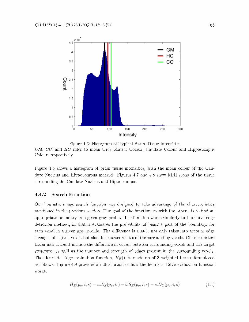
CHAPTER 4. CREATING THE ASM 65
Figure 4.6: Histogram of Typical Brain Tissue IntensitiesGM, CC, and HC refer to mean Grey Matter Colour, Caudate Colour and HippocampusColour, respectively.
Figure 4.6 shows a histogram of brain tissue intensities, with the mean colour of the Cau-
date Nucleus and Hippocampus marked. Figures 4.7 and 4.8 show MRI scans of the tissue
surrounding the Caudate Nucleus and Hippocampus.
4.4.2 Search Function
Our heuristic image search function was designed to take advantage of the characteristics
mentioned in the previous section. The goal of the function, as with the others, is to �nd an
appropriate boundary in a given grey pro�le. The function works similarly to the naïve edge
detection method, in that it evaluates the probability of being a part of the boundary, for
each voxel in a given grey pro�le. The di�erence is that it not only takes into account edge
strength of a given voxel, but also the characteristics of the surrounding voxels. Characteristics
taken into account include the di�erence in colour between surrounding voxels and the target
structure, as well as the number and strength of edges present in the surrounding voxels.
The Heuristic Edge evaluation function, HE(), is made up of 3 weighted terms, formulated
as follows. Figure 4.9 provides an illustration of how the heuristic Edge evaluation function
works.
HE(pv, i, s) = a.ES(pv, i, )− b.SE(pv, i, s)− c.DC(pv, i, s) (4.4)

CHAPTER 4. CREATING THE ASM 66
Figure 4.7: MRI Scan of Caudate NucleusThe sagittal MRI scan shows a manually-traced Left Caudate Nucleus in red.
Figure 4.8: MRI Scan of HippocampusThe sagittal MRI scan shows a manually-traced Left Hippocampus in red.

CHAPTER 4. CREATING THE ASM 67
ES(), SE(), and DC() refer to Edge Score, Sample Edges, and Di�erence in Colour, re-
spectively. These terms will be discussed in detail in the following section.
Once the voxel with the highest heuristic Edge score in pv has been detected, the per-vertex
adjustment is computed in a similar fashion to the edge detection image search method. Vertex
v is moved along surface normal in the direction of the voxel with the highest Heuristic Edge
score, for a distance proportional to the Heuristic Edge score of that voxel.
Edge Score
The Edge Score term, ES(pv, i), uses a simple 1D convolution kernel to �nd the edge strength
of a given voxel, i, as it appears in a grey pro�le, pv. This term operates in a similar fashion
to the edge detection image search method mentioned earlier. The term is weighted by the
constant a. This weighting allows for the adjustment of the contribution that each term has
on the �nal score. This concept is discussed in further detail in Section 4.4.5.
Sample Edges
The Sample Edges term, SE(pv, i, s), sums the total strength of all edges that are present in a
sample that appears immediately to the right of voxel i in grey pro�le pv. The sample length
is speci�ed as s. This term e�ectively measures inhomogeneity in the sample to the right of
the voxel in question. This measure is based on the assumption that the Caudate Nucleus
and Hippocampus are relatively homogeneous, and is therefore negatively weighted by the
constant −b.The sample is taken to the right hand side of voxel i because of the direction in which grey
pro�les are sampled along local surface normals. The surface normal orientation is such that
the left hand side of grey pro�les always point towards the outside of the target structure, and
the right hand side always points towards the inside.
This term, when negatively weighted and combined with the previous Edge Score term,
detects edges that are bordered to the right by homogeneous regions - as one would expect to
�nd around the borders of the target structures.
Di�erence in Colour
The Di�erence in Colour term, DC(pv, i, s), measures the di�erence between the mean colour of
a sample - also taken to the right of the ith voxel - and the mean colour of the target structure
being segmented. The mean colour of the target structure is determined via a lengthy process
that is explained in detail in Section 4.4.3.
Based on the assumption that the Caudate Nucleus is generally darker than the surround-
ing areas, the Di�erence in Colour term only penalises the Heuristic Edge score if the sample
mean is lighter than the mean Caudate colour. The Caudate tail is also known to be darker

CHAPTER 4. CREATING THE ASM 68
Figure 4.9: Heuristic Edge evaluationpv is a typical grey pro�le sample, taken from a Caudate Nucleus target volume. CC indicatesthe mean Caudate colour, as detected by our algorithm. Using the naïve edge detectionmethod, voxel i = 8 would have been incorrectly chosen (it is on the wrong side of the targetstructure), since it has the strongest edge value. However, the heuristic edge detection methodtakes into account the homogeneity of the voxels i = 3 to i = 7 (to the right of the sample),as well as the fact that the mean colour of these voxels is close to that of the Caudate Nucleusin this target volume - resulting in i = 2 being correctly chosen as the boundary of the targetstructure.
than the rest of the structure, so the mean Caudate colour is multiplied by 0.7 when the
vertex, v, corresponding to the grey pro�le pv, is part of the tail.
The area surrounding the Hippocampus can be both lighter and darker than the Hip-
pocampal mean colour. So, instead of only penalising the Heuristic Edge score for the sample
mean being lighter, in the case of the Hippocampus, the Di�erence in Colour term calculates
the absolute value of the di�erence between the sample mean and the Hippocampus mean -
thus incurring a penalty for the sample mean being either darker or lighter.
The Di�erence in Colour term is also negatively weighted, using the constant −c.
4.4.3 Target Colour Determination
The heuristic edge detection method relies largely on the knowledge of the mean tissue intensity
of the target structure. In order to determine this intensity, we employ a lengthy algorithm,
based mainly on a method devised by Worth et al, and to a lesser degree on the method
employed by Xia et al [42, 44]. These methods are discussed next. Following this discussion,
we describe each step of our method in detail. We then evaluate the e�ectiveness of our
method.

CHAPTER 4. CREATING THE ASM 69
Algorithm 4.4 Xia's Tissue Intensity Determination Algorithm
1. Calculate histogram
2. Smooth histogram using Fourier decomposition
(a) Perform Fourier transform of histogram
(b) Cut o� high frequency Fourier components
(c) Perform inverse Fourier transform
3. Identify peaks of tissue classes
(a) Model tissue classes as sum of normal Gaussian functions
(b) Fit tissue model to smoothed histogram using least squares error �t
4. Determine thresholds of tissue classes
Figure 4.10: Histogram Smoothing using Fourier decompositionElimination of high frequency Fourier components leads to unwanted low frequency artifacts.
Current Methods
Xia et al extract the Cerebral Ventricular System from MR Images by �rst determining the in-
tensities of white matter, grey matter and cerebrospinal �uid, and then using a region-growing
approach to segment ROIs. Tissue intensity determination is achieved using Algorithm 4.4.
We found that the use of Fourier decomposition for histogram smoothing left us with
unwanted low frequency peaks. This is illustrated in Figure 4.10. Smoothing can instead be
achieved using a discrete convolution with a Gaussian kernel. Peak identi�cation can also be
done without the use of the computationally-intensive least squares error �t technique.
Worth et al make use of Algorithm 4.5 to identify the tissue intensity of the Caudate
Nucleus. This algorithm is part of a heuristic algorithm that is used to segment out the
Caudate Nucleus and Lateral Ventricles. Note that Step 4d is only necessary to model the
approximate shape of an entire peak. The midpoint and approximate area of the peak can be
determined without �tting a Gaussian function to it.

CHAPTER 4. CREATING THE ASM 70
Algorithm 4.5 Worth's Tissue Intensity Determination Algorithm
1. Isolate brain area from non-brain area, using a Talairach atlas
2. Remove strong edge voxels
(a) Use a Sobel edge �lter to detect strong edges
(b) Remove strong edges, leaving relatively homogeneous areas only
3. Calculate histogram of brain area (global histogram)
4. Determine peaks in global histogram
(a) Convolve histogram with derivative of a Gaussian
(b) Locate negative-going zero crossings in graph of �rst derivative, indicating peaks
(c) Calculate peak area, excluding peaks below a certain threshold
(d) Fit a Gaussian shaped function to each detected peak in the histogram
5. Locate Corpus Callosum using heuristic method
6. Identify boxes surrounding Caudate Nucleus and Ventricles, using Corpus Callosum aslandmark
7. Calculate histogram of Caudate Nucleus and Ventricles (local histogram)
8. Determine peaks in local histogram
(a) Use the same method as Step 4 to determine peaks
(b) Identify the peak that is slightly below the highest intensity peak, and of slightlygreater intensity than the global grey matter peak, as belonging to the CaudateNucleus

CHAPTER 4. CREATING THE ASM 71
Target Volume Preprocessing
In order to remove scanning artifacts and other spurious voxels from the target volume, a
�ood �ll is �rst performed on the background area, outside of the skull boundary. The �ood
�ll isolates the volume contained in the skull from the rest of the voxels, allowing for a more
accurate global histogram.
The next step is to crop the volume to begin on the skull boundary. This is achieved by
casting rays from the original target volume borders, vertically and horizontally, towards the
centre of the volume. The point in each axis at which the rays �rst intersect with the skull
is taken as the cropping plane for that axis. The cropped volume allows faster processing of
subsequent steps, as the volume to be processed becomes smaller.
The �nal preprocessing step is to remove strong edges using a Sobel �lter. A 2D Sobel
�lter is convolved with each slice of the target volume to identify edges. Edges with scores
above a certain threshold are then removed, leaving behind areas of relatively homogeneous
intensity, and containing only weak gradients.
These preprocessing steps are illustrated in Figure 4.11.
Global Peak Detection
The �rst step in peak detection is to calculate the global histogram of voxel intensities for
the target volume - with the background voxels thresholded out. This histogram is initially
quite jagged, and must be smoothed to be useful. Smoothing is achieved by convolving the
histogram with a discrete Gaussian convolution kernel. This smoothing step is repeated a
number of times, depending on the width of the histogram. The width of the histogram is
proportional to the range of intensities present in the target volume. If the volume contains
only a small range of intensities, then smoothing the histogram too many times will cause too
much loss of information, rendering it useless. Thus, the range of intensities is �rst determined,
and the histogram is then smoothed accordingly.
The next step is identify peaks in the smoothed histogram. This is done by �rst convolving
the histogram with a discrete Gaussian �rst derivative kernel. This convolution produces an
approximation of the �rst derivative of the histogram. The �rst derivative approximation is
then smoothed using the original Gaussian kernel. Peaks can now be identi�ed by negative-
going zero crossings of the �rst derivative function.
Because of the inherently jagged nature of the histogram and its approximate �rst deriva-
tive, many peaks will be identi�ed by looking for zero crossings. In order to eliminate false
positives, the area of each of these peaks must be determined. Peak area is determined in a
similar way to Worth's method of adding the absolute values of the heights of the �rst deriva-
tive of the histogram on each side of the negative-going zero crossing [42]. Instead of adding
the heights, we sum the area under the curve at each discrete point in the histogram, between

CHAPTER 4. CREATING THE ASM 72
the two zero crossings. Using this method, we can express the area of a peak as a proportion
of the total histogram area - simply calculated by summing the area under the curve at each
point in the full histogram. Peaks with areas that are proportionally much smaller than the
histogram itself, are discarded as false positives. Through trial and error, we found that valid
peaks are usually greater than 130 th of the total histogram area.
At this point, there should be 2-3 peaks of interest left, since the dark cerebrospinal �uid
can sometimes be thresholded out during the process. The grey matter peak is always the
second last peak of the remaining group. This grey matter value should be saved for later
comparison to the local grey matter colour, since this is the peak of interest in our segmentation
algorithm. Figure 4.11 illustrates the peak detection process.
Local Peak Detection
Now that the global grey matter intensity has been determined, a similar process must be un-
dertaken to �nd the grey matter intensity local to the area surrounding the target structure.
Since both the Caudate Nucleus and Hippocampus consist entirely of grey matter, determin-
ing this intensity will provide the necessary information for the Di�erence in Colour term
mentioned previously.
The �rst step in determining local intensity is to isolate the area surrounding the target
structure. Worth's method involves a lengthy heuristic procedure involving locating the Corpus
Callosum, and using this as a landmark to �nd the Caudate Nucleus. This procedure is
unnecessary in our algorithm, as we already have information regarding the mean location
of target structures, as recorded in our training shapes. Indeed, our method already relies
on this location to initialise the ASM prior to segmentation. Using the mean location and
orientation of the training shapes we can reliably determine the bounding boxes surrounding
both the Caudate Nuclei and Hippocampi in a given target volume. This is done based on the
previously mentioned assumption that target data will be captured in a similar orientation to
the training data used to create the ASM.
After the target structure has been isolated, the algorithm proceeds to calculate peaks
using the same method as was used to determine global peaks. Again, the second last peak
that remains after �ltering is taken to be the local grey matter intensity. This peak is checked
against the global grey matter peak to ensure that it is of a slightly higher intensity.
In some cases, the target volume is of such poor contrast that determination of the local
grey matter peak fails. In these situations, local grey matter intensity is estimated based on
global grey matter intensity. Based on our previous assumptions, grey matter belonging to
the Caudate Nucleus and Hippocampus would be estimated at 1.25 and 1.17 times the global
grey matter intensity, respectively.

CHAPTER 4. CREATING THE ASM 73
Figure 4.11: Caudate Colour DeterminationCC indicates the �nal Caudate Colour. CSF, GM and WM indicate cerebrospinal �uid, greymatter and white matter, respectively.
Evaluation
Caudate Nucleus and Hippocampus colour determination algorithms were tested in the fol-
lowing fashion. The algorithm was run on each unsegmented target volume, and the global
grey matter and target structure colours were recorded. These colours were then compared
to the mean target structure colour in the corresponding segmented volume. The results are
summarised in Table 4.3.
GM Guessing refers to the estimation of target structure intensity, based on the detected
global grey matter intensity. When the algorithm fails to determine the local grey matter
intensity (often due to poor contrast data), or the algorithm determines an intensity that is
outside of an acceptable range, the intensity is estimated according to the previously mentioned
assumptions about the ratio between target structure and global grey matter intensity.
A colour estimate is deemed to be a false positive when the algorithm does not fail (i.e.
falsely indicates success), but provides an estimate that is outside of the acceptable range of
intensities for a particular target structure - based on the mean target structure intensity, as
determined from manually segmented test data. False positives are detectable in most cases,
by measuring whether the ratio between global grey matter intensity and local grey matter
intensity is within acceptable limits. In very few cases (2 out of 62, for the Caudate Nucleus,
and 0 out of 52, for the Hippocampus), these false positives went undetected, and would

CHAPTER 4. CREATING THE ASM 74
Caudate Nucleus Hippocampus
No Samples 62 52
Success W/O GM Guessing 47% 98%
Success W GM Guessing 82% 98%
Mean Intensity 88.95 80.96
Min Intensity 40 36
Max Intensity 130 109
False Positives 4 1
False Pos Rate 6% 2%
Detected False Pos 2 1
Undetected False Pos 2 0
Undetected False Pos Rate 3% 0%
Table 4.3: Results of Evaluation of Target Colour Determination
therefore cause poor segmentation results.
The results show that the Target Colour Determination algorithm works satisfactorily for
Caudate Nucleus target structures, with an 82% success rate. In cases where the algorithm
fails, the ASM segmentation method would have to be altered to not rely on the knowledge of
the target structure colour. This can be achieved by assigning a weighting of 0 to the Di�erence
in Colour term. Fortunately these failures are mostly detectable, and can be compensated for.
The algorithm works exceptionally well in determining the colour of target Hippocampi.
With a 98% success rate, and only 1 false positive (which was detectable), the results show
that the algorithm is very reliable when applied to these structures.
4.4.4 Multisampling
A frequently occurring problem during ASM segmentation is the tendency of grey pro�le
samples to occasionally miss the boundary that is being searched for by a small margin. The
surface normal used for grey sampling on either side of a speci�ed vertex, v, may not intersect
with a desired boundary - resulting in the vertex being attracted to an incorrect place in the
target volume.
In order to address this issue, provision was made for taking multiple samples along vectors
at a slight angle to the surface normal of a particular vertex. Given an angle, θ, and a desired
number of samples, t, the optimal adjustment is calculated according to Algorithm 4.6.
Multisampling therefore increases the chance of detecting more suitable boundaries during
segmentation. It is theorised that this would work especially well for the heuristic method,
since it is not only formulated to search for boundaries based on a naïve measure, such as edge
strength (strong boundaries do not always signify target structure borders), but for boundaries
that are characteristic of the target structure. Figure 4.12 is an illustration of multisampling.

CHAPTER 4. CREATING THE ASM 75
Algorithm 4.6 Multisampling
1. Sample pv along surface normal
2. Evaluate HE(pv, i, s), and store value x0
3. For n = 0 to t− 1
(a) Sample pv along vector at angle θ to surface normal, rotated by 2πnt
(b) Evaluate HE(pv, i, s), and store value xn+1
4. Find max(x0..n+1), and calculate adjustment using sample with highest score
Figure 4.12: Multisamplingt = 4 extra samples are taken, at an angle θ = π
16 .

CHAPTER 4. CREATING THE ASM 76
4.4.5 Parameter �nding using a Genetic Algorithm
The heuristic edge detection algorithm relies on the use of various parameters to control
segmentation. These parameters are detailed below.
� Pro�le length (l). This parameter determines the length of sampled grey pro�les, pv.
Typical values range between 3 and 5.
� Sample length (s). This determines the sample length, as detailed in Section 4.4.2.
Typical values range between 3 and 7.
� Term weighting (a, b, c). These parameters control relative term weighting, as detailed
in Section 4.4.2. Typical values range between 0.5 and 6.0.
� Maximum edge value (m). This parameter controls the maximum expected boundary
edge value. This varies according to target structure, and is used to control the propor-
tional adjustment of vertices in the search function. The Caudate Nucleus tends to have
stronger boundaries than the Hippocampus, and will thus require higher values of m.
Typical values range between 50 and 500.
In order to maximise segmentation accuracy, it is necessary to �nd the best set of parameters
for each target structure. Parameters that work well for Caudate Nucleus segmentation do not
necessarily work as well for Hippocampus segmentation. In order to test a set of parameters,
a segmentation must be run using them. Since the target volume data vary in brightness,
contrast, and signal-to-noise ratio, it is not enough to merely test a set of parameters on one
target volume. A set of parameters must therefore be used in multiple segmentation runs
to test its e�ectiveness. This process is considerably time consuming, and it is not feasible
to experiment with all possible parameter combinations, as the search space is fairly large.
Assuming a discrete parameter intervals of 1 for parameters l and s, 0.5 for parameters a,b,
and c, and 50 for parameter m, there are 3 ∗ 5 ∗ 12 ∗ 12 ∗ 12 ∗ 10 = 259200 possible sets of
parameters. Evaluation of a parameter set over 10 target volumes takes approximately 27
minutes in MATLAB (running on one CPU of a 2.66GHz Intel Core2 Duo E6750), resulting
in a total time of approximately 6998400 minutes to explore the entire search space.
Since exhaustive exploration of the parameter search space was infeasible, we use a GA
to �nd the best set of parameters for each target structure. The GA was implemented in
MATLAB, and proceeds according to Algorithm 4.7. The initial population was chosen at
random. The formulation and results of our GA are discussed in the following sections.
Encoding
Individual genes in our GA chromosomes simply represent segmentation parameters. The
chromosomes therefore consist of 6 genes each. Genes consist of integer indexes ranging from

CHAPTER 4. CREATING THE ASM 77
Algorithm 4.7 GA Processing
1. Generate initial population of n individuals
2. While generations < maximum generations, repeat:
(a) Selection, selecting n2 pairs of parents
(b) Crossover, generating n new children
(c) Mutation of new children
3. Store �ttest 10 individuals for further evaluation
Algorithm 4.8 GA Fitness Function
1. Create ASM
2. Translate gene encodings into ASM parameters
3. Run segmentation on representative target volumes
(a) Segment volume
(b) Evaluate segmentation overlap against manual segmentation
4. Fitness value is the mean segmentation overlap over entire target volume set
1 to the maximum number of discrete intervals in the range of values for their respective
parameters. For example, the chromosome [1 2 3 6 5 4] represents the parameter values [l = 3
s = 4 a = 1.5 b = 3.0 c = 2.5 m = 200].
Evaluation
The �tness function takes a chromosome, evaluates it, and returns a scalar �tness value.
Segmentation overlap, as detailed in Chapter 5, was used as our �tness metric. A separate
�tness function was used to evaluate the two target structure types, since Caudate Nucleus
segmentation is slightly di�erent to Hippocampus evaluation. Each �tness function follows
the same general algorithm (see Algorithm 4.8).
Selection
In order for a new generation to be born at the end of an epoch, pairs of parents need
to be chosen from the population. In order to direct evolution, the selection must favour
�tter individuals. Roulette Wheel selection is used to achieve this. Each individual's �tness
represents a portion of the total �tness of the population. Individuals with higher �tness
are represented by a larger portion of the �tness distribution. A random point along this

CHAPTER 4. CREATING THE ASM 78
chrom. l s a b c maxedge Fitness LC30 σL RC30 σR
1 3 6 3 1 2 300 0.854 0.804 0.09 0.800 0.08
2 3 6 3 1 3 300 0.853 0.807 0.08 0.805 0.07
3 4 5 2.5 2 3 350 0.853 0.796 0.09 0.781 0.07
4 4 5 1.5 1.5 4 300 0.852 0.782 0.09 0.757 0.08
5 4 5 1 1 5 350 0.852 0.772 0.10 0.764 0.07
6 3 5 4 3.5 3 450 0.851 0.790 0.10 0.752 0.09
7 4 5 1 1 5.5 300 0.850 0.762 0.11 0.758 0.08
8 3 6 3 1 4.5 450 0.850 0.804 0.09 0.805 0.06
9 4 5 2 2 3 400 0.850 0.784 0.10 0.762 0.07
10 4 5 2.5 2 5 300 0.850 0.798 0.08 0.770 0.06
Table 4.4: 10 Fittest Caudate Nucleus ChromosomesFitness is the result of the �tness function. LC30 and RC30 refer to the mean overlap recordedby running the parameters on the 30 left and right Caudate Nucleus test data, respectively.σL and σR refer to the standard deviation of the left and right overlap data, respectively.Chromosome 2 has the highest combined mean, and lowest combined standard deviation.
distribution is chosen. The individual represented by that point is then selected for procreation.
This allows �tter individuals to have a greater chance of producing o�spring, thereby increasing
the overall �tness of the population.
Crossover and Mutation
After two parents procreate, two new individuals are �born�. There is a chance that these
two individuals will be exactly the same as their parents, and a chance that their genes will
�cross over� to form new chromosomes based on both of the parents' genes. This chance is
represented by a variable called crossover rate. A random point along the chromosome is
chosen. Genes to the left of that point come from the one parent, whilst genes to the right
come from the other. For the second child, crossover also happens at the same point, but
parents are swapped.
The mutation process is fairly simple. The mutation algorithm iterates through the chro-
mosome from left to right. At each gene, it generates a random number. If this number is less
than the speci�ed mutation rate, the gene is replaced with a new one. The replacement gene is
generated randomly, and must be within the range speci�ed for its corresponding parameter.
Results
Optimum results were achieved with a crossover rate of 70% and a mutation rate of 20%. A
population size of n = 20 was used, and the algorithm ran for 100 generations. The �ttest 10
individuals were recorded for each target structure. These results are detailed in Tables 4.4
and 4.5.

CHAPTER 4. CREATING THE ASM 79
chrom. l s a b c maxedge Fitness LH26 σL RH26 σR
1 4 6 2 1 5 100 0.778 0.753 0.05 0.776 0.06
2 3 5 2 1 5.5 100 0.773 0.749 0.04 0.772 0.05
3 4 5 1 0.5 5.5 100 0.772 0.741 0.05 0.761 0.06
4 3 6 3 1 5 100 0.772 0.758 0.05 0.775 0.05
5 4 6 2.5 1 5.5 150 0.771 0.744 0.06 0.775 0.05
6 4 5 1 0.5 5 100 0.770 0.738 0.05 0.762 0.06
7 4 6 2 1 3.5 200 0.770 0.729 0.07 0.773 0.05
8 4 6 1.5 0.5 3 100 0.769 0.752 0.05 0.770 0.06
9 3 5 3 1 5.5 100 0.766 0.738 0.05 0.729 0.04
10 4 6 3.5 1.5 5.5 150 0.764 0.730 0.06 0.773 0.05
Table 4.5: 10 Fittest Hippocampus ChromosomesFitness is the result of the �tness function. LC26 and RC26 refer to the mean overlap recordedby running the parameters on the 26 left and right Hippocampus test data, respectively. σL andσR refer to the standard deviation of the left and right overlap data, respectively. Chromosome4 has the highest combined mean, and lowest combined standard deviation.
Each of the 10 �ttest chromosomes were then evaluated in a full test run of 30 and 26
target volumes, in the case of the Caudate Nucleus and Hippocampus, respectively. For each
target structure, the set of parameters that generated the best overall results was used in the
�nal evaluation - detailed in Chapter 5.

Chapter 5
Evaluation
In this chapter, we strive to evaluate the e�ectiveness of the ASM segmentation techniques on
the test data used in the study into the neural correlates of FASD (detailed in Section 3.1).
These data are representative of the data expected to be segmented in the future of this study,
and conclusions can therefore be drawn regarding the e�ectiveness of using our technique for
that purpose.
Throughout development of the segmentation algorithm, qualitative measures such as 3D
plots of ASM mesh deformation and 2D MRI slices have been used to evaluate the e�ective-
ness of the technique. Despite being useful for development and debugging, these qualitative
measures rely on subjective interpretation, and can thus be misleading. Therefore, in or-
der to scienti�cally evaluate segmentation success, we present only results generated using
quantitative measures in this evaluation chapter.
We present this chapter in two sections. Firstly, we discuss the quantitative metrics used for
evaluation. Secondly, we discuss the results generated by these metrics, and draw conclusions
about the e�ectiveness of our technique.
5.1 Metrics
In this section, we discuss the background and our implementation of the quantitative metrics
used for evaluation. These metrics include commonly-used segmentation measures such as
overlap and segmentation error. Metrics such as volume di�erence and surface area di�erence
o�er an easy-to-calculate, but naïve measure of segmentation success. They are not widely
used, and are therefore excluded from this evaluation.
5.1.1 Overlap
The overlap metric, ε, is used to measure the fraction of possible voxels shared by two binary
segmentations. It is formulated as follows [44].
80

CHAPTER 5. EVALUATION 81
ε =2V12
(V1 + V2)(5.1)
V1 and V2 are the scalar volume measures of the two binary segmentations in question.
V12 is the scalar volume of the intersection of V1and V2. Thus, ε represents the ratio of actual
overlap to possible overlap. For our purposes, the overlap metric is used to measure the success
of our segmentation algorithm in identifying a target structure in a target data volume. Thus,
V1will represent the scalar volume measure of the manually segmented ground truth data
volume, G. V2 thus indicates the scalar volume measure of the automatically segmented data
volume, A. V12 is the scalar volume measure of the intersection of A and G, A ∩G, and can
also be represented as VA∩G. This metric is used widely in segmentation literature, and can
therefore be used as an objective comparison of segmentation results between similar studies
[44, 19, 46, 11].
False positive and false negative ratios can be calculated in a similar fashion. False posi-
tives, or overestimated voxels, are those voxels that have been erroneously identi�ed as being
part of the target structure. These voxels can be described as the relative complement of
A, given G, or A − G. The volume of false positives, VA−G, and the ratio of false positives
to volume of overlap,VA−G
VA∩G, are also commonly-used metrics [44]. False negatives, or missed
voxels, can be described as the relative complement of G, given A, or G − A. Similarly, the
volume of false negatives, VG−A, and the ratio of false negatives to volume of overlap,VG−A
VA∩G,
are frequently used [44]. False positives and negatives can also be expressed somewhat more
intuitively as a proportion of the target volume, formulated asVA−G
VGand
VG−A
VG, respectively.
Implementation
Since our ASM takes the form of a deformable 3D surface mesh, and the overlap metric takes
two binary volumes as input, it is necessary to discretise the surface mesh into a group of
voxels. This is achieved by rendering the mesh to the target volume, and marking each voxel
that is interior to the mesh, using Algorithm 5.1. The mesh is of a much higher resolution
than the target volume, and fully enclosed volume is generated in step 2.
After mesh discretisation, we are left with binary target volume A, and manually segmented
binary volume G. These isotropic volumes each contain 1mm3 voxels, thus making volume
calculation simply a matter of counting the voxels with value 1. It is then a simple process to
calculate overlap, ε = 2VA∩G(VA+VG) , volume of false positives, VA−G, and volume of false negatives,
VG−A.

CHAPTER 5. EVALUATION 82
Algorithm 5.1 Mesh-to-Volume Conversion
1. Create an empty binary volume, equal in size to the target volume
2. For each vertex, v, of the �tted ASM mesh
(a) Determine which voxel in the binary volume is intersected by v
(b) Set the intersected voxel to 1
3. For each slice in the z-plane of the binary volume
(a) For each row, set voxels with value 0 to 1 (voxels must be enclosed on both sidesby a voxel with value 1, that is not already part of a �lled extent)
(b) For each column, repeat step 3a
5.1.2 Segmentation Error
Average segmentation error, discussed in Section 3.3.2, is a measure of the mean distance
between each vertex of a �tted mesh, MA, and the closest point in a mesh generated from a
manually segmented ground truth data volume, MG. The mean-squared distance, mentioned
in Section 2.2.2 is used more often than mean distance, as squaring the di�erence generates
more noticeable results.
One advantage of using these metrics is that, as well as measuring the total di�erence
between all vertices, it is also possible to measure the di�erence between subsets of vertices -
thereby allowing closer scrutiny of surface overlap in localised regions, such as the tail of the
Caudate Nucleus, for example.
Hausdor� distance can also be used to measure how successfully the ASM has been �tted
to target data [28, 6]. This metric measures the maximum error between the boundaries of
the ground truth mesh, MG and the �tted mesh, MA.
It is also useful to measure the standard deviation of distances between vertices ofMA and
the target, MG. This re�ects the regularity of the segmentation results. Results with a high
standard deviation would indicate an erratic segmentation, which is undesirable.
Implementation
We used the Matlab isosurface routine to generate surface meshes of manually segmented
ground truth volumes. Strictly speaking, segmentation error metrics should measure the
distances between each vertex of a �tted mesh, and the nearest point on a target surface.
However, since our meshes are of much higher resolution than our 1mm3 target data, it is
su�cient to measure the distance between each vertex in MA and the closest vertex in MG.
In order to ensure fair results, MG is tessellated to be at least double the resolution of MA.

CHAPTER 5. EVALUATION 83
5.2 Results
In this section, we present the results of our evaluation. Firstly we discuss the evaluation
methods and test data used. Secondly, we discuss the evaluation of the ASM in terms of
segmentation ability, using the overlap and segmentation error metrics.
5.2.1 Method and Materials
Our test data consisted of 30 MRI brain volumes with manually segmented left and right
Caudate Nuclei, as well as 26 manually segmented left and right Hippocampi. As previously
mentioned, these data are taken from a study into the neural correlates of FASD. More detailed
information, such as scanning parameters, is available in Section 3.1.
These data were used both as manually segmented �ground truth� volumes, and as unseg-
mented target volumes to test ASM segmentation ability. In order to ensure unbiased results,
each unsegmented target volume was segmented using an ASM that was built using leave-
one-out construction. Thus, no ASM was evaluated using test data that it was initially built
from. This was done to emulate the real-world use case where the ASM is used on previously
unsegmented data.
5.2.2 Evaluating Segmentation Ability
In the following sections, we discuss the evaluation of the segmentation ability of our ASM.
The evaluation goal was to test the comparative e�ectiveness of segmentation using the four
di�erent image search methods. These included the naïve edge detection method, the grey
pro�le Mahalanobis distance method, the heuristic method, and the heuristic method with
multisampling.
ASMs based on the four target structures were constructed for this evaluation. These in-
cluded ASMs for left and right Caudate Nuclei, as well as ASMs for left and right Hippocampi.
For each target structure, ASMs were constructed using varying numbers of training shapes.
This was done to evaluate the e�ect that adding more training data to the ASMs had on
the segmentation results. The Caudate ASMs were constructed with 10, 20 and 30 training
shapes. The Hippocampus ASMs were constructed with 10, 20 and 26 training shapes. Thus,
12 ASMs were evaluated in total (4 structures × 3 variations in the number of training shapes
used).
For each of these ASMs, Algorithm 5.2 was used to evaluate the ability of the ASM to
segment unseen test data. As mentioned, data were considered unseen since each ASM was
built using leave-one-out construction.
Segmentation metrics used in this section included:
� Overlap

CHAPTER 5. EVALUATION 84
Algorithm 5.2 Evaluation of ASM Segmentation Ability
1. For i = 1..Ns
(a) Construct ASM from Ns training shapes, leaving shape i out
(b) For each segmentation method, M (Edge Detection, grey pro�le Mahalanobis dis-tance, heuristic method, heuristic method with multisampling):
i. Initialise ASM
ii. Segment unsegmented target data volume i, using segmentation method M
iii. Evaluate segmentation metrics for target volume i, method M
� Ratio of false positives to overlap
� Ratio of false negatives to overlap
� Mean-squared distance
� Hausdor� distance
� Standard deviation of distances
Full evaluation results can be found in Appendix A.
5.2.3 Normality Testing
In order to facilitate certain further statistical analysis, normality testing was performed on the
results. This was done to each result set by �rst �nding the mean and standard deviation of a
Gaussian distribution that most closely matched the histogram of results, and then measuring
the correlation coe�cient to determine how strongly the results are correlated to the standard
normal distribution.
Normality testing was performed on the overlap metric results of segmentation using each
image search method, for each target structure. Correlation results are summarised in Table
5.1. Correlation coe�cient values indicate a strong correlation (0.5 < r < 1.0) between all
results histograms and the standard normal distribution. We can therefore conclude that our
results are normally distributed.
Graphical plots of Gaussian distributions �tted to Left Caudate results histograms can be
seen in Figure 5.1.
5.2.4 Outliers
An outlier is de�ned as an experimental result that di�ers markedly from the other results
in the set. When a set of results follows a known distribution, it is relatively easy to spot

CHAPTER 5. EVALUATION 85
Figure 5.1: Normality TestingNormal Distributions (red) are �tted to histograms of segmentation overlap results (blue). ED,GPM, H, and HM refer to the image search methods: edge detection, grey pro�le Mahalanobis,heuristic, and heuristic with multisampling. Outliers are indicated in green.

CHAPTER 5. EVALUATION 86
Left Caudate Right Caudate
ED r = 0.7766, µ = 0.77, σ = 0.05 r = 0.9420, µ = 0.77, σ = 0.04
GPM r = 0.7410, µ = 0.69, σ = 0.1 r = 0.6683, µ = 0.72, σ = 0.07
H r = 0.8971, µ = 0.84, σ = 0.03 r = 0.9390, µ = 0.83, σ = 0.04
HM r = 0.9749, µ = 0.84, σ = 0.03 r = 0.9163, µ = 0.84, σ = 0.04
(a) Caudate Nuclei
Left Hippocampus Right Hippocampus
ED r = 0.5439, µ = 0.66, σ = 0.09 r = 0.8930, µ = 0.66, σ = 0.06
GPM r = 0.5811, µ = 0.43, σ = 0.17 r = 0.7692, µ = 0.65, σ = 0.08
H r = 0.8838, µ = 0.8, σ = 0.02 r = 0.9458, µ = 0.8, σ = 0.03
HM r = 0.8614, µ = 0.77, σ = 0.04 r = 0.8373, µ = 0.77, σ = 0.03
(b) Hippocampi
Table 5.1: Normality TestingED, GPM, H, and HM refer to edge detection, grey pro�le Mahalanobis, heuristic, and heuris-tic with multisampling. r is the correlation coe�cient. µ and σ refer to the mean and standarddeviation of the Gaussian distribution that most closely approximated the results histogram.
outliers, as they do not correspond to the expected distribution of results. Since our results
follow a normal distribution, it is possible to work out the probability that a given result is a
member of the sampled population of results, or not. Based on this probability, outliers can
be identi�ed and removed, so as to avoid results that are not representative of the population
that is being sampled.
Chauvenet's Criterion was used to identify and remove outliers in our data [36]. According
to Chauvenet, an experimental result can be rejected as an outlier if the probability of obtaining
the result (based on the number of standard deviations from the mean) is less than 12n , where
n is the number of results.
As with normality testing, we performed outlier identi�cation based on overlap results for
each image search method, tested on each ASM type. Table 5.2 lists the target volumes with
overlap results identi�ed as outliers, per results set. Figure 5.1 shows outliers in the Left
Caudate Nucleus result set. Full results, including and excluding outliers, are available in
Appendix A.
From the Caudate Nucleus results, it can be seen that target volume 6 is particularly ill-
suited to segmentation. Except for the image search using grey pro�le Mahalanobis distance
on the right Caudate Nucleus, overlap results for volume 6 are statistically too poor to prob-
abilistically �t into a normal distribution. This is likely due to poor contrast, low brightness,
or a low signal-to-noise ratio - causing segmentation to fail. Similarly, but to a lesser degree,
target volume 8 seems to not be particularly suited to Hippocampal segmentation using the
heuristic image search method (with and without multisampling). Conversely, segmentation of
the Right Hippocampus in target volume 1, using the 10-shape ASM, results in an improbably

CHAPTER 5. EVALUATION 87
ED GPM H HM
Ns = 10 {6} {6} {6} {6}
Ns = 20 {6} {6} {6} {6}
Ns = 30 {6} {6} {6} {6}
(a) Left Caudate Nuclei
ED GPM H HM
Ns = 10 {6} {} {6} {}
Ns = 20 {6} {8} {6} {6,12}
Ns = 30 {6,30} {4,8} {6} {6,12}
(b) Right Caudate Nuclei
ED GPM H HM
Ns = 10 {} {} {} {}
Ns = 20 {} {} {8} {8}
Ns = 26 {} {} {} {}
(c) Left Hippocampi
ED GPM H HM
Ns = 10 {1} {3} {} {8}
Ns = 20 {} {} {8} {8}
Ns = 26 {} {} {8} {}
(d) Right Hippocampi
Table 5.2: Outlier Results Identi�ed per Results SetED, GPM, H, and HM refer to the image search methods: edge detection, grey pro�le Ma-halanobis, heuristic, and heuristic with multisampling. Numbers in braces refer to resultsnumbers identi�ed as outliers, e.g. {6,8} indicates that the overlap results for target volumes6 and 8 were identi�ed as outliers.

CHAPTER 5. EVALUATION 88
Figure 5.2: Segmentation Failure of Target Volume 6The �rst image shows a 2D slice through target volume 6, with the ill-�tted ASM outlined inblack. Note the low contrast and blurriness of the image. These scanning artifacts are usuallycaused by movement in the subject. The second image shows a 3D representation of the ASM(red) and the target ROI (blue).
excellent result, and is therefore eliminated.
Out of 232 results, 37 outliers where identi�ed - giving an outlier percentage of 37232 ×
1001 =
15.9%. 20 of the 37 outliers occurred due to segmentation failure of target volume 6 - this
accounts for 20232×
1001 = 8.6% of the total number of of results. Figure 5.2 shows segmentation
failure of the left Caudate Nucleus ASM on target volume 6.
5.2.5 Paired Di�erence Test for Statistical Signi�cance
In order to draw a meaningful conclusion about the di�erence in segmentation results, it is
necessary to �rst prove that the results di�er enough to infer statistical signi�cance. We aim to
draw conclusions regarding the comparative e�ectiveness of the various image search methods

CHAPTER 5. EVALUATION 89
used in our ASM. In order to do this, we evaluate the di�erence in mean segmentation results
using these various methods.
We use a paired di�erence test for statistical signi�cance, aiming to disprove the null
hypothesis that the means of two sets of segmentation results are not statistically di�erent.
Again, we used the overlap metric as our basis for comparison of results, since this metric is
the most representative of the e�ectiveness of the image search methods in question. Since
outliers have been eliminated, not all sets of results could be paired for comparison. Thus,
we performed the dependent t-test only on samples that had corresponding pairs in all results
sets. The test was performed using a signi�cance level of 5%. Full results can be found in
Appendix A. A summary of results for ASMs with the largest number of training shapes is
presented in Table 5.3.
5.2.6 Segmentation Results and Discussion
Table 5.4 lists a summary of segmentation results for ASMs with the largest number of training
shapes (i.e. Ns = 30 for Caudate Nuclei, and Ns = 26 for Hippocampi). Full results are
available in Appendix A.
In the following sections we compare results for the 6 di�erent segmentation metrics, and
draw conclusions about the relative e�ectiveness of the various image search methods. For the
sake of brevity, from now on, we refer to the heuristic image search method by their respective
acronyms.
Overlap Results
Beginning with the overlap metric, it is clear, from Table 5.3 and Table 5.4, that for all
four target structures, the heuristic method (with and without multisampling) signi�cantly
outperformed both the ED and the GPM methods. The use of the heuristic method with
multisampling generated higher mean overlap results for Caudate Nucleus target volumes,
than the use of the heuristic method without multisampling. However, the mean di�erence
between the two sets of results is statistically insigni�cant, and thus no conclusion can be
drawn as to the comparative e�ectiveness of the use of multisampling in this case. When
comparing these two methods on Hippocampus targets, we recorded a statistically signi�cant
improvement in the use of the heuristic method without multisampling. This leads us to the
conclusion that multisampling creates at best an insigni�cant di�erence in results, and at
worst a decrease in segmentation e�ectiveness. This decrease in e�ectiveness is probably due
to the higher likelihood of vertices being attracted to strong, but incorrect boundaries when
multisampling is used.
The GPM method performs worst out of the four image searches. When compared to the
previous chapter's initialisation statistics (Table 4.2), it is important to note that the GPM

CHAPTER 5. EVALUATION 90
µ σ n t-stat p(T<=t) signi�cant
ED-H 0.08 0.06 29 7.18 <0.001 TRUE
ED-HM 0.08 0.06 29 7.54 <0.001 TRUE
GPM-H 0.15 0.09 29 9.12 <0.001 TRUE
GPM-HM 0.16 0.09 29 9.13 <0.001 TRUE
H-HM 0 0.03 29 0.91 0.371239 FALSE
(a) Left Caudate Nuclei
µ σ n t-stat p(T<=t) signi�cant
ED-H 0.07 0.07 25 5.13 <0.001 TRUE
ED-HM 0.08 0.06 25 6.04 <0.001 TRUE
GPM-H 0.12 0.12 25 5.13 <0.001 TRUE
GPM-HM 0.13 0.11 25 5.68 <0.001 TRUE
H-HM 0.01 0.02 25 1.17 0.252708 FALSE
(b) Right Caudate Nuclei
µ σ n t-stat p(T<=t) signi�cant
ED-H 0.19 0.11 26 9.23 <0.001 TRUE
ED-HM 0.18 0.1 26 8.82 <0.001 TRUE
GPM-H 0.26 0.13 26 10.45 <0.001 TRUE
GPM-HM 0.24 0.12 26 10.42 <0.001 TRUE
H-HM 0.01 0.03 26 2.47 0.020669 TRUE
(c) Left Hippocampi
µ σ n t-stat p(T<=t) signi�cant
ED-H 0.13 0.06 23 10.33 <0.001 TRUE
ED-HM 0.09 0.08 23 5.45 <0.001 TRUE
GPM-H 0.15 0.08 23 8.81 <0.001 TRUE
GPM-HM 0.11 0.09 23 5.55 <0.001 TRUE
H-HM 0.04 0.04 23 4.85 <0.001 TRUE
(d) Right Hippocampi
Table 5.3: Results of Paired Di�erence TestED, GPM, H, and HM refer to the image search methods: edge detection, grey pro�le Maha-lanobis, heuristic, and heuristic with multisampling, e.g. ED-H refers to the di�erence betweenedge detection and heuristic image search methods. µ and σ refer to the mean di�erence andstandard deviation of di�erences. n is the sample size, while t-stat refers to the t-test statisticvalue. p(T<=t) refers to the two-tail p value.

CHAPTER 5. EVALUATION 91
Overlap FP Ratio FN Ratio MSD Hausdor� SDD
ED 0.74 0.49 0.13 0.97 3.76 0.63
GPM 0.67 0.26 0.37 1.79 4.09 0.83
H 0.82 0.16 0.2 0.75 2.7 0.49
HM 0.82 0.14 0.2 0.74 2.63 0.49
(a) Left Caudate Nuclei
Overlap FP Ratio FN Ratio MSD Hausdor� SDD
ED 0.75 0.42 0.16 0.84 3.28 0.59
GPM 0.69 0.28 0.32 1.28 3.72 0.73
H 0.81 0.14 0.21 0.76 2.73 0.48
HM 0.82 0.13 0.21 0.78 2.59 0.47
(b) Right Caudate Nuclei
Overlap FP Ratio FN Ratio MSD Hausdor� SDD
ED 0.57 0.69 0.32 2.19 4.83 1.05
GPM 0.5 0.46 0.51 2.82 4.76 1.04
H 0.76 0.3 0.21 0.73 3.1 0.56
HM 0.75 0.28 0.24 0.87 3.28 0.59
(c) Left Hippocampi
Overlap FP Ratio FN Ratio MSD Hausdor� SDD
ED 0.65 0.78 0.16 1.7 4.62 0.97
GPM 0.64 0.43 0.33 1.59 3.97 0.84
H 0.79 0.25 0.19 0.72 2.82 0.52
HM 0.74 0.29 0.25 0.99 3.35 0.63
(d) Right Hippocampi
Table 5.4: Summary of Mean Segmentation ResultsED, GPM, H, and HM refer to the image search methods: edge detection, grey pro�le Ma-halanobis, heuristic, and heuristic with multisampling. Overlap, False Positive (FP) Ratio,False Negative (FN) Ratio, Mean Squared Distances (MSD), Hausdor� Distance and StandardDeviation of Distances (SDD) segmentation metric means are displayed in the correspondingcolumns.
CHAPTER 5. EVALUATION 92
method actually generates a worse segmentation over time. All other methods tend to improve
their mean overlap as segmentation proceeds. This indicates a fundamental �aw with the use
of the GPM method in this context. This is possibly due to boundary inhomogeneities in our
training data. This is discussed towards the end of this section.
False Positive and False Negative Ratios
As previously discussed, False Positive Ratio and False Negative Ratio refer to the ratio of
false positives and false negatives to the volume of overlap, respectively. Our results indicate
that although the ED method generated acceptable overlap results, it had a tendency to over-
segment the data. This is apparent from the fact that mean false positive ratios were very
high, whilst mean false negative ratios remained low for all target structures. In fact, in all
target structures except the Left Hippocampus, the ED method generated the lowest mean
false negative ratios. The same method also generated the highest mean false positive ratios
in all four target structures.
The GPM method generated poor mean false positive and false negative ratios for all target
structures. This indicates that the area segmented by this method was more or less uniformly
o�set from the target structure. This lack of precision once again indicates a �aw in the use
of the GPM method, and this is discussed later.
The heuristic method (with and without multisampling) signi�cantly outperformed both
the ED and GPM methods in terms of mean false positive ratios for all structures, indicating a
uniform tendency to avoid over- and under-segmentation. However, the ED method generated
slightly lower false negative ratios for three of the structures. There was no large di�erence in
ratios when using the heuristic method with or without multisampling.
Segmentation Error Metrics
As expected, mean squared distances are approximately inversely proportional to overlap.
Results for the GPMmethod show the highest mean squared distances in most cases, indicating
that the model boundary was situated relatively far from the target boundary. Again, the ED
method gives moderate results, whilst the heuristic method without multisampling gives the
best results - resulting in an average mean squared distance of under 1mm2 in all cases.
The Hausdor� distance results are much the same, indicating that the maximum segmen-
tation error was, in most cases, lowest for the heuristic method without multisampling. The
ED and GPM methods fared the worst in all cases.
Standard Deviation of Distances indicates a large �uctuation in model-vertex-to-target-
boundary distances for the ED and GPM methods. This indicates erratic segmentation results,
with some vertices situated close to target boundaries, and some situated far away. Again,
the heuristic method without multisampling showed reliable consistency in segmentation, with

CHAPTER 5. EVALUATION 93
Min Max Median
LC 0.65 0.88 0.83
RC 0.65 0.88 0.82
LH 0.66 0.82 0.78
RH 0.72 0.85 0.79
Table 5.5: Min, Max and Median Overlap for the Heuristic MethodLC, RC, LH and RH represent the four target structures: Left Caudate Nucleus, RightCaudate Nucleus, Left Hippocampus, Right Hippocampus.
the lowest mean standard deviation of distances results in all cases.
Number of Training Shapes
In order to determine the optimal number of training shapes to use in ASM construction, we
compared the overlap results generated by ASMs constructed from varying training set sizes.
Figure 5.3 and 5.4 show this comparison.
For the ED, H and HM methods, the 30- and 26- shape ASMs performed best. This was
not the case with the GPM method, which performed best using 20-shape ASMs.
FreeSurfer Validity Study
A recent study was done into the validity of using the FreeSurfer software package for mea-
surement of brain volumes in children with fetal alcohol syndrome [17]. This study was done
using the same MRI test data that we used in our experiments.
The study reported inter-observer correlations for manual tracings of target structures
ranging from r = 0.94 to r = 0.99, with a median of r = 0.98. This inter-observer correlation
indicates the high reliability of the manually delimited target volumes used in our study.
The FreeSurfer package automatically reconstructs an entire cortical surface, and corre-
sponding sub-cortical volumes from an MRI brain volume. This process is time-consuming,
as target structures can not be segmented individually. Results from the FreeSurfer study
indicate that manual tracings are highly correlated with automatically segmented volumes.
Correlation coe�cient values ranged from a worst case of rs = 0.74 for the Right Hippocam-
pus to a best case of rs = 0.89 for the total Caudate, with a median of 0.83.
Since overlap is directly proportional to correlation, we can compare the FreeSurfer correla-
tions with our overlap results. Table 5.5 shows median and maximum results for our heuristic
method that are similar to the FreeSurfer correlations, although minimum values were signif-
icantly lower for most structures. These results indicate that our heuristic method is a viable
alternative to FreeSurfer. Also, when segmenting individual target structures, our method
takes around 5 to 10 minutes, whereas FreeSurfer typically takes 24 to 36 hours on equivalent

CHAPTER 5. EVALUATION 94
(a) Left Caudate Nuclei
(b) Right Caudate Nuclei
Figure 5.3: ASM Training Set Size vs Overlap results for Caudate NucleiED, GPM, H, and HM refer to the image search methods: edge detection, grey pro�le Maha-lanobis, heuristic, and heuristic with multisampling.

CHAPTER 5. EVALUATION 95
(a) Left Hippocampi
(b) Right Hippocampi
Figure 5.4: ASM Training Set Size vs Overlap results for HippocampiED, GPM, H, and HM refer to the image search methods: edge detection, grey pro�le Maha-lanobis, heuristic, and heuristic with multisampling.

CHAPTER 5. EVALUATION 96
hardware (due to the whole-brain segmentation). Thus, when used for rapid segmentation of
individual target structures, our method may be preferable to the use of FreeSurfer.
GPM Image Search Failure
The GPM image search method failed to detect boundaries e�ectively. This failure was prob-
ably due to the relative heterogeneity of organ boundaries in our training data. As explained
in Section 4.3.2, the GPM method relies on a strong correlation between greyscale intensities
of corresponding boundary points in training data. If this correlation is not strong enough
(due to noise or contrast factors, for example) the GPM method fails to create a good model
of the boundary surrounding a target shape. Without a decent model of the boundary, the
GPM image search fails to attract vertices to boundaries, and produces a bad segmentation.
Figure 5.3 and 5.4 show that more training data leads to worse GPM performance. This
supports the notion that boundary models become more homogenous, and thus worse for
boundary identi�cation, with more data.
5.3 Conclusion
During this evaluation, we used a wide range of segmentation metrics to evaluate the e�ec-
tiveness of the various image search methods when applied to the data from the study into
FASD. The results were shown to follow a standard normal distribution. This fact allowed for
the elimination of outliers, and for the use of a paired di�erence test to determine whether the
di�erences in sets of results were large enough to be statistically signi�cant.
This statistical analysis showed that the heuristic method without multisampling was con-
sistently better at segmenting our target data than other image search methods. The use of
multisampling was at best equivalent to the use of the heuristic method without multisam-
pling, and since multisampling requires extra computation, it is therefore better to use the
heuristic method by itself. The edge detection method produced average results, although it
showed a tendency to over-segment the target data. The grey pro�le Mahalanobis method
fared the worst of the four. This failure was ascribed to heterogeneity in training data. The
heuristic method also showed the lowest standard deviation in results, again showing reliable
consistency in segmentation. Other methods produced somewhat more erratic results.
Results from the heuristic method were favourable when compared to results of automatic
segmentation of the same data using the FreeSurfer software package. Although the FreeSurfer
results were slightly better, the ASM approach allows for independent target structure seg-
mentation, and is therefore much less computationally demanding. Thus, individual target
segmentation using the heuristic method is much faster, and may be preferable to the use of
FreeSurfer. Both FreeSurfer and the heuristic method provide a lower level of accuracy when

CHAPTER 5. EVALUATION 97
compared to manual segmentation. Since the FreeSurfer method has been used in numerous
studies, such as the one mentioned in the previous section, and our results are comparable
to those produced by FreeSurfer, we conclude that the heuristic method provides su�cient
accuracy to be used in similar FASD-related studies.
In order to improve segmentation results, whilst maintaining most of the speed bene�t, it
may be possible to use the heuristic ASM method as the initial stage in a semi-automatic seg-
mentation process - the fast initial automatic segmentation would then be manually corrected
by neuroanatomists. This would result in dramatically improved accuracy, at a marginal cost
of a few minutes of segmentation time.

Chapter 6
Conclusion and Future Work
The aim of this research was to perform an objective comparison of classical and currently
popular ASM techniques, in order to �nd the algorithm that is most suitable to segmenting
the Caudate Nucleus and Hippocampus structures from the data used in a study into FASD.
In order to achieve this objective, the following three tasks were undertaken: landmark point
generation, Active Shape Model (ASM) construction, and experimental evaluation. These tasks,
as well as the work undertaken to achieve them, will be summarised next. This will be followed
by a summary of results, and a discussion on possible future work.
6.1 Tasks
This research project was comprised of three primary tasks.
6.1.1 Landmark Point Generation
This task was to �nd and implement an e�cient and e�ective method of assigning 3D land-
mark points to volumetric training data. Landmark points are a necessary prerequisite to ASM
construction. This task was addressed by designing and implementing a Geometrically De-
formable Model (GDM) based on MacDonald's approach [23], but optimised for performance
and segmentation quality when used with Magnetic Resonance Imaging (MRI) data generated
as part of our study into FASD. Optimisations included the use of a kd-tree for proximity
detection, and triangle-triangle intersection tests, amongst others. The GDM implementation
was evaluated in terms of performance and segmentation quality. A full discussion of the
implementation and evaluation of the GDM is provided in Chapter 3.
98

CHAPTER 6. CONCLUSION AND FUTURE WORK 99
6.1.2 ASM Construction
The goal was to create ASMs using di�erent image search techniques, in order to facilitate
objective evaluation of their e�ectiveness in segmentation of the Caudate Nucleus and Hip-
pocampus from our test data. This was achieved by �rstly constructing a basic ASM, and
�nding the best initialisation method suited to our data. Various popular ASM image search
techniques were implemented, in order to compare their e�ectiveness. A heuristic method of
image search was designed and implemented to take advantage of speci�c characteristics of the
target structures of interest in our test data. An addition was made to the heuristic method,
which enabled the use of multisampling during the image search phase. ASM parameter �nd-
ing was undertaken using a Genetic Algorithm. Full details of this ASM construction process
are provided in Chapter 4.
6.1.3 Experimental Evaluation
The goal was to set up and conduct experiments to determine the ASM implementation that
produced the best segmentation results. This was achieved by �rstly adding automatic eval-
uation features into the ASM implementations to measure popular metrics, such as overlap
and segmentation error. Statistical validation of results, including normality testing, outlier
elimination, and paired di�erence testing, was then performed. Statistical analysis of segmen-
tation results was performed, allowing us to draw objective conclusions about the success of
various image search techniques. Full details of this analysis are available in Chapter 5.
6.2 Summary of Results
Normality testing showed that segmentation results were strongly correlated to the Standard
Normal Distribution, with correlation coe�cients ranging from r = 0.5439 to r = 0.9749.
Thirty-seven outliers were identi�ed using Chauvenet's Criterion, and removed from 232 re-
sults. Paired di�erence tests with a con�dence level of 5% allow us to draw the following
conclusions regarding segmentation results.
In terms of mean segmentation overlap, the heuristic method without multisampling con-
sistently outperformed other image search methods. Overlap values were 0.82, 0.81, 0.76 and
0.79 for the Left Caudate Nucleus, Right Caudate Nucleus, Left Hippocampus, and Right
Hippocampus, respectively.
The heuristic method combined with multisampling produced, at best, equivalent over-
lap results to the heuristic method without multisampling (0.82, 0.82, 0.75, 0.74 for the Left
Caudate Nucleus, Right Caudate Nucleus, Left Hippocampus, and Right Hippocampus, re-
spectively).
The heuristic method (with and without multisampling) vastly outperformed both the

CHAPTER 6. CONCLUSION AND FUTURE WORK 100
edge detection (ED) and grey pro�le Mahalanobis (GPM) method in terms of false positive
ratios, whilst the ED method produced the best false negative ratios.
The GPM method fared worst out of the four image search methods tested, both in terms
of overlap and in terms of false positive and false negative ratios. This failure was ascribed to
heterogeneity in training data.
Mean squared distances were approximately inversely proportional to overlap results. Re-
sults for the GPM method show the highest mean squared distances in most cases, indicating
that the model boundary was situated relatively far from the target boundary. The ED method
gave moderate results, whilst the heuristic method without multisampling gave the best results
- resulting in an average mean squared distance of under 1mm2 in all cases.
The heuristic method without multisampling generated segmentation results with the low-
est standard deviation, allowing us to conclude that it is the most reliable method of the four.
The method is not perfect - segmentation did fail on some data sets. However, this segmenta-
tion failure was usually due to extreme noise or low contrast. Thus, we can conclude that the
heuristic method without multisampling displays acceptable reliability for the segmentation
of current and expected future data to be used in the FASD study.
Automatic segmentation using an ASM based on our heuristic method produces compa-
rable results to those produced by the FreeSurfer software package. The ASM method is less
computationally intensive, as it is able to segment individual target structures, whilst the
FreeSurfer package focuses on segmenting the entire brain. Therefore, the ASM method takes
around 5 to 10 minutes to complete a segmentation, whereas FreeSurfer typically takes 24
to 36 hours on equivalent hardware. Thus, although results are not always as good as those
produced by FreeSurfer, the ASM approach may be preferable in terms of computation time.
It may also be bene�cial to use our ASM method as an initial, rapid, automatic segmentation
step, which could then be manually corrected - resulting in a fast and accurate semi-automatic
segmentation method.
All-in-all, our method will allow for more rapid segmentation of the Caudate Nucleus and
Hippocampus structures, thereby accelerating research into FASD. This important research
will allow us to better understand the neural correlates of this debilitating disorder.
6.3 Future Work
There are a number of areas in which our work has and can be extended.
6.3.1 GDM Use
Our GDM implementation has been used in study on Hippocampus shape variation in children
with FASD [3]. It will also be used in a similar future study into Caudate Nucleus shape

CHAPTER 6. CONCLUSION AND FUTURE WORK 101
variation.
6.3.2 ASM Use and Evaluation
Further investigation can be done into the use of non-Euclidean ASM shape descriptors, such
as the Minimum Description Length (MDL) approach [10, 9], mapping to Spherical Harmonics
(SPHARM) [19], and mapping to Spherical Wavelet Basis functions [28]. These methods have
been shown to increase ASM e�ectiveness in certain cases, and could possibly provide better
segmentation results.
A more general ASM framework for research into segmentation would be useful. Currently,
ASMs must be created from scratch, and there is no easy way for researchers to compare the
e�ectiveness of various ASM construction techniques. A modular, pluggable framework would
enable researchers to experiment with combinations of di�erent ASM construction techniques
in order to �nd the best implementation for their particular study.
An application should be made using the ASM techniques experimented with in this study.
This application would allow researchers to automatically or semi-automatically segment tar-
get structures, thereby contributing to the study into FASD. In order to make segmentation
quick and robust, it may be preferable to use the heuristic ASM technique as the initial step
in a semi-automatic segmentation process. A quick initial segmentation, followed by manual
veri�cation and correction of any possible errors would be the ideal combination of speed and
accuracy for the FASD study.

Bibliography
[1] M. Brejl and M. Sonka. Object localization and border detection criteria design inedge-
based image segmentation: automated learning from examples. Medical Imaging, IEEE
Transactions on, 19(10):973�985, 2000.
[2] J. Canny. A computational approach to edge detection. Pattern Analysis and Machine
Intelligence, IEEE Transactions on, 8(6):679�698, 1986.
[3] J. Christopher, A. Eicher, C. Warton, S. Jacobson, C. Molteno, J. Jacobson, P. Marais,
and E. Meintjes. Surface deformation-based analysis of regional shape variations of hip-
pocampus in children with FAS. In Proceedings of the Joint Annual Meeting ISMRM-
ESMRMB, 2010.
[4] T.F. Cootes, C.J. Taylor, D.H. Cooper, J. Graham, et al. Active shape models-their
training and application. Computer Vision and Image Understanding, 61(1):38�59, 1995.
[5] G.J. Bailey B.A. Jacobson S.J. Delaney-Black V. Cortese, B.M. Moore and J.H. Hanni-
gan. Magnetic resonance and spectroscopic imaging in prenatal alcohol-exposed children:
Preliminary �ndings in the caudate nucleus. Neurotoxicology and Teratology, 28(5):597 �
606, 2006.
[6] F.A. Cosío. Automatic initialization of an active shape model of the prostate. Medical
Image Analysis, 12(4):469�483, 2008.
[7] C. Davatzikos, X. Tao, and D. Shen. Hierarchical active shape models, using the wavelet
transform. Medical Imaging, IEEE Transactions on, 22(3):414�423, 2003.
[8] R.H. Davies. Learning shape: optimal models for analysing natural variability. Citeseer,
2002.
[9] R.H. Davies, C.J. Twining, P.D. Allen, T.F. Cootes, and C.J. Taylor. Shape discrimination
in the hippocampus using an MDL model. Information Processing in Medical Imaging,
4, 2003.
102

BIBLIOGRAPHY 103
[10] R.H. Davies, C.J. Twining, T.F. Cootes, J.C. Waterton, and C.J. Taylor. A minimum
description length approach to statistical shape modeling. Medical Imaging, IEEE Trans-
actions on, 21(5):525�537, 2002.
[11] M. de Bruijne, B. van Ginneken, W.J. Niessen, J.B.A. Maintz, and M.A. Viergever. Active
shape model based segmentation of abdominal aortic aneurysms in CTA images. In Proc.
SPIE, volume 4684, pages 463�474, 2002.
[12] D.H. Eberly. 3D game engine design: a practical approach to real-time computer graphics.
Morgan Kaufmann Pub, 2001.
[13] P.A. Freeborough, N.C. Fox, and R.I. Kitney. Interactive algorithms for the segmen-
tation and quantitation of 3-D MRI brain scans. Computer Methods and Programs in
Biomedicine, 53(1):15�25, 1997.
[14] A. Ghanei, H. Soltanian-Zadeh, and J.P. Windham. A 3D deformable surface model for
segmentation of objects from volumetric data in medical images. Computers in Biology
and Medicine, 28(3):239�253, 1998.
[15] J.C. Gower. Generalized Procrustes Analysis. Psychometrika, 40(1):33�51, 1975.
[16] P.V.C Hough. A Method and Means for Recognizing Complex Patterns, 1962. US Patent
3,069,654.
[17] C. Jacobson, S.W. nad Warton, N.C. Dodge, F. de Guio, C. Molteno, J.L Jacobson, and
E. Meintjes. Validity of FreeSurfer for measurement of brain volumes in children with
fetal alcohol syndrome. In Proceedings of 16th Annual Meeting of the Organization for
Human Brain Mapping (OHBM), 2010.
[18] M. Kass, A. Witkin, and D. Terzopoulos. Snakes: Active contour models. International
journal of computer vision, 1(4):321�331, 1988.
[19] A. Kelemen, G. Szekely, and G. Gerig. Elastic model-based segmentation of 3-D neuro-
radiological data sets. Medical Imaging, IEEE Transactions on, 18(10):828�839, 1999.
[20] J.M. Lee, S.H. Kim, D.P. Jang, T.H. Ha, J.J. Kim, I.Y. Kim, J.S. Kwon, and S.I. Kim.
Deformable model with surface registration for hippocampal shape deformity analysis in
schizophrenia. Neuroimage, 22(2):831�840, 2004.
[21] W.W. Lee, I. Richardson, K. Gow, Y. Zhao, and R. Sta�. Hybrid Segmentation of the
Hippocampus in MR Images. European Signal Processing Conference (EUSIPCO), 2005.

BIBLIOGRAPHY 104
[22] W.E. Lorensen and H.E. Cline. Marching cubes: A high resolution 3D surface construc-
tion algorithm. Proceedings of the 14th annual conference on Computer graphics and
interactive techniques, pages 163�169, 1987.
[23] D. MacDonald, N. Kabani, D. Avis, and A.C. Evans. Automated 3-D Extraction of Inner
and Outer Surfaces of Cerebral Cortex from MRI. Neuroimage, 12(3):340�356, 2000.
[24] P.C. Mahalanobis. On the generalized distance in statistics. In Proceedings of the National
Institute of Science, Calcutta, volume 12, page 49, 1936.
[25] P. Marais. Introduction to computer vision and image processing.
[26] J.V. Miller, D.E. Breen, W.E. Lorensen, R.M. O'Bara, and M.J. Wozny. Geometrically
deformed models: a method for extracting closed geometric models from volume data.
SIGGRAPH Comput. Graph., 25(4):217�226, 1991.
[27] T. Moller. A fast triangle-triangle intersection test. Journal of graphics tools, 2(2):25�30,
1997.
[28] D. Nain, S. Haker, A. Bobick, and A. Tannenbaum. Multiscale 3-d shape representation
and segmentation using spherical wavelets. Medical Imaging, IEEE Transactions on,
26(4):598, 2007.
[29] J. Pantel, D.S. O'Leary, K. Cretsinger, H.J. Bockholt, H. Keefe, V.A. Magnotta, and
N.C. Andreasen. A New Method for the In Vivo Volumetric Measurement of the Human
Hippocampus With High Neuroanatomical Accuracy. Hippocampus, 10(6), 2000.
[30] D.L. Pham, C. Xu, and J.L. Prince. A survey of current methods in medical image
segmentation. Annual Review of Biomedical Engineering, 2:315�337, 2000.
[31] R.A. Pooley. Fundamental Physics of MR Imaging 1. RadioGraphics, 25(4):1087�1099,
2005.
[32] F.J. Rohlf and D. Slice. Extensions of the Procrustes method for the optimal superimpo-
sition of landmarks. Syst. Zool, 39(1):40�59, 1990.
[33] D. Shen, E.H. Herskovits, and C. Davatzikos. An adaptive-focus statistical shape model
for segmentation and shape modeling of 3-D brain structures. Medical Imaging, IEEE
Transactions on, 20(4):257�270, 2001.
[34] L.I. Smith. A tutorial on principal components analysis. Unpublished, 2002.
[35] M. Sonka, V. Hlavac, and R. Boyle. Image Processing, Analysis and Machine Vision,
Second Edition. Brooks/Cole, Thomson Asia Pte Led, United State of America.

BIBLIOGRAPHY 105
[36] J.R. Taylor. An introduction to error analysis: the study of uncertainties in physical
measurements. Univ Science Books, 1997.
[37] A. Tsai, W. Wells, C. Tempany, E. Grimson, and A. Willsky. Mutual information in
coupled multi-shape model for medical image segmentation. Medical Image Analysis,
8(4):429�445, 2004.
[38] J.K. Udupa and G.T. Herman. 3D Imaging in Medicine. CRC Press, Inc. Boca Raton,
FL, USA, 1991.
[39] H. William, S.A. Teukolsky, W.T. Vetterling, and B.P. Flannery. Numerical Recipes in C:
The art of scienti�c computing. Cambridge university press New York, NY, USA, 1988.
[40] R. Dyson M. Williams, P.L. Warwick and L.H. Bannister. Gray's anatomy.
[41] R.P. Woods. Multitracer: a Java-based tool for anatomic delineation of grayscale volu-
metric images. NeuroImage, 19(4):1829�1834, 2003.
[42] A.J. Worth, N. Makris, M.R. Patti, J.M. Goodman, E.A. Hoge, VS Caviness, and D.N.
Kennedy. Precise segmentation of the lateral ventricles and caudate nucleus in MR brain
images using anatomically driven histograms. Medical Imaging, IEEE Transactions on,
17(2):303�310, 1998.
[43] Y. Xia, K. Bettinger, L. Shen, and A.L. Reiss. Automatic Segmentation of the Cau-
date Nucleus From Human Brain MR Images. Medical Imaging, IEEE Transactions on,
26(4):509�517, 2007.
[44] Y. Xia, Q. Hu, A. Aziz, and W.L. Nowinski. A knowledge-driven algorithm for a rapid
and automatic extraction of the human cerebral ventricular system from MR neuroimages.
Neuroimage, 21(1):269�282, 2004.
[45] P. Yan and A.A. Kassim. Medical Image Segmentation Using Minimal Path Deformable
Models With Implicit Shape Priors. Information Technology in Biomedicine, IEEE Trans-
actions on, 10(4):677�684, 2006.
[46] P.A. Yushkevich, J. Piven, H.C. Hazlett, R.G. Smith, S. Ho, J.C. Gee, and G. Gerig. User-
guided 3D active contour segmentation of anatomical structures: Signi�cantly improved
e�ciency and reliability. Neuroimage, 31(3):1116�1128, 2006.

Appendix A
Results
Results Summary
Left Caudate Nucleus
The following tables show means and standard deviations of segmentation results, for ASMs
built with 10-30 shapes, after elimination of outliers. MSD refers to the mean squared distance,
SDD to standard deviation of distances.
10 Shapes, Means
Method Overlap FP-Ratio FN-Ratio MSD Hausdor� SDD
Edge 0.74 0.48 0.14 1.06 4.05 0.68
Mahalanobis 0.71 0.35 0.25 1.32 4.13 0.76
Heuristic 0.82 0.18 0.18 0.67 2.76 0.48
Heur-Multi 0.82 0.16 0.19 0.73 2.75 0.5
10 Shapes, Standard Deviations
Method Overlap FP-Ratio FN-Ratio MSD Hausdor� SDD
Edge 0.05 0.13 0.06 0.52 1.7 0.24
Mahalanobis 0.06 0.15 0.06 0.85 1.45 0.31
Heuristic 0.03 0.1 0.06 0.19 0.64 0.08
Heur-Multi 0.03 0.1 0.06 0.23 0.43 0.07
106

APPENDIX A. RESULTS 107
20 Shapes, Means
Method Overlap FP-Ratio FN-Ratio MSD Hausdor� SDD
Edge 0.74 0.51 0.12 0.96 3.91 0.64
Mahalanobis 0.72 0.3 0.28 1.3 3.58 0.69
Heuristic 0.82 0.18 0.19 0.71 2.84 0.49
Heur-Multi 0.82 0.16 0.19 0.71 2.62 0.48
20 Shapes, Standard Deviations
Method Overlap FP-Ratio FN-Ratio MSD Hausdor� SDD
Edge 0.07 0.23 0.05 0.59 1.83 0.23
Mahalanobis 0.09 0.19 0.11 0.82 1.43 0.27
Heuristic 0.05 0.12 0.06 0.19 0.67 0.08
Heur-Multi 0.04 0.09 0.06 0.18 0.43 0.07
30 Shapes, Means
Method Overlap FP-Ratio FN-Ratio MSD Hausdor� SDD
Edge 0.74 0.49 0.13 0.97 3.76 0.63
Mahalanobis 0.67 0.26 0.37 1.79 4.09 0.83
Heuristic 0.82 0.16 0.2 0.75 2.7 0.49
Heur-Multi 0.82 0.14 0.2 0.74 2.63 0.49
30 Shapes, Standard Deviations
Method Overlap FP-Ratio FN-Ratio MSD Hausdor� SDD
Edge 0.07 0.22 0.05 0.65 1.57 0.22
Mahalanobis 0.09 0.28 0.12 1.18 1.5 0.29
Heuristic 0.04 0.11 0.05 0.21 0.52 0.08
Heur-Multi 0.03 0.08 0.05 0.17 0.43 0.07
Right Caudate Nucleus
The following tables show means and standard deviations of segmentation results, for ASMs
built with 10-30 shapes, after elimination of outliers. MSD refers to the mean squared distance,
SDD to standard deviation of distances.

APPENDIX A. RESULTS 108
10 Shapes, Means
Method Overlap FP-Ratio FN-Ratio MSD Hausdor� SDD
Edge 0.72 0.48 0.16 1.15 3.8 0.71
Mahalanobis 0.62 0.41 0.36 1.91 4.58 0.96
Heuristic 0.78 0.19 0.22 0.82 2.97 0.54
Heur-Multi 0.77 0.16 0.26 0.82 2.86 0.53
10 Shapes, Standard Deviations
Method Overlap FP-Ratio FN-Ratio MSD Hausdor� SDD
Edge 0.05 0.13 0.06 0.84 1.1 0.27
Mahalanobis 0.1 0.17 0.15 1.15 1.29 0.3
Heuristic 0.07 0.12 0.13 0.33 0.68 0.13
Heur-Multi 0.11 0.1 0.17 0.29 0.77 0.13
20 Shapes, Means
Method Overlap FP-Ratio FN-Ratio MSD Hausdor� SDD
Edge 0.73 0.45 0.16 0.95 3.4 0.63
Mahalanobis 0.67 0.27 0.35 1.32 3.84 0.77
Heuristic 0.8 0.17 0.23 0.8 2.83 0.5
Heur-Multi 0.81 0.15 0.21 0.77 2.64 0.47
20 Shapes, Standard Deviations
Method Overlap FP-Ratio FN-Ratio MSD Hausdor� SDD
Edge 0.06 0.13 0.06 0.49 0.91 0.19
Mahalanobis 0.11 0.19 0.14 0.87 1.11 0.28
Heuristic 0.06 0.08 0.1 0.3 0.67 0.11
Heur-Multi 0.04 0.08 0.06 0.22 0.38 0.06
30 Shapes, Means
Method Overlap FP-Ratio FN-Ratio MSD Hausdor� SDD
Edge 0.75 0.42 0.16 0.84 3.28 0.59
Mahalanobis 0.69 0.28 0.32 1.28 3.72 0.73
Heuristic 0.81 0.14 0.21 0.76 2.73 0.48
Heur-Multi 0.82 0.13 0.21 0.78 2.59 0.47

APPENDIX A. RESULTS 109
30 Shapes, Standard Deviations
Method Overlap FP-Ratio FN-Ratio MSD Hausdor� SDD
Edge 0.05 0.13 0.05 0.38 0.78 0.15
Mahalanobis 0.1 0.2 0.14 0.87 0.86 0.26
Heuristic 0.06 0.07 0.08 0.25 0.59 0.09
Heur-Multi 0.04 0.06 0.08 0.25 0.45 0.08
Left Hippocampus
The following tables show means and standard deviations of segmentation results, for ASMs
built with 10-26 shapes, after elimination of outliers. MSD refers to the mean squared distance,
SDD to standard deviation of distances.
10 Shapes, Means
Method Overlap FP-Ratio FN-Ratio MSD Hausdor� SDD
Edge 0.55 0.7 0.34 2.39 4.99 1.06
Mahalanobis 0.44 0.59 0.54 4.05 5.43 1.17
Heuristic 0.75 0.35 0.18 0.8 3.63 0.64
Heur-Multi 0.76 0.34 0.19 0.76 3.65 0.61
10 Shapes, Standard Deviations
Method Overlap FP-Ratio FN-Ratio MSD Hausdor� SDD
Edge 0.13 0.16 0.2 1.42 1.26 0.28
Mahalanobis 0.16 0.15 0.2 3.49 2.01 0.51
Heuristic 0.06 0.15 0.08 0.39 1.46 0.26
Heur-Multi 0.06 0.15 0.08 0.4 1.28 0.23
20 Shapes, Means
Method Overlap FP-Ratio FN-Ratio MSD Hausdor� SDD
Edge 0.56 0.7 0.32 2.29 4.9 1.07
Mahalanobis 0.52 0.46 0.48 2.75 4.92 1.04
Heuristic 0.76 0.29 0.21 0.74 3.02 0.56
Heur-Multi 0.74 0.29 0.24 0.85 3.23 0.58

APPENDIX A. RESULTS 110
20 Shapes, Standard Deviations
Method Overlap FP-Ratio FN-Ratio MSD Hausdor� SDD
Edge 0.11 0.14 0.17 1.24 1.22 0.32
Mahalanobis 0.12 0.15 0.14 2.32 1.56 0.43
Heuristic 0.04 0.14 0.07 0.2 0.61 0.11
Heur-Multi 0.05 0.09 0.08 0.33 0.73 0.11
26 Shapes, Means
Method Overlap FP-Ratio FN-Ratio MSD Hausdor� SDD
Edge 0.57 0.69 0.32 2.19 4.83 1.05
Mahalanobis 0.5 0.46 0.51 2.82 4.76 1.04
Heuristic 0.76 0.3 0.21 0.73 3.1 0.56
Heur-Multi 0.75 0.28 0.24 0.87 3.28 0.59
26 Shapes, Standard Deviations
Method Overlap FP-Ratio FN-Ratio MSD Hausdor� SDD
Edge 0.11 0.15 0.19 1.18 1.19 0.3
Mahalanobis 0.12 0.15 0.14 2.15 1.5 0.43
Heuristic 0.05 0.12 0.07 0.21 0.7 0.12
Heur-Multi 0.04 0.11 0.07 0.24 0.64 0.1
Right Hippocampus
The following tables show means and standard deviations of segmentation results, for ASMs
built with 10-26 shapes, after elimination of outliers. MSD refers to the mean squared distance,
SDD to standard deviation of distances.
10 Shapes, Means
Method Overlap FP-Ratio FN-Ratio MSD Hausdor� SDD
Edge 0.64 0.78 0.16 1.62 4.46 0.98
Mahalanobis 0.59 0.64 0.31 2.06 4.34 0.91
Heuristic 0.77 0.29 0.2 0.81 2.96 0.55
Heur-Multi 0.8 0.23 0.19 0.68 2.78 0.49

APPENDIX A. RESULTS 111
10 Shapes, Standard Deviations
Method Overlap FP-Ratio FN-Ratio MSD Hausdor� SDD
Edge 0.04 0.17 0.07 0.42 0.97 0.27
Mahalanobis 0.07 0.3 0.12 1.19 1.11 0.3
Heuristic 0.08 0.18 0.1 0.49 0.82 0.23
Heur-Multi 0.03 0.09 0.08 0.27 0.56 0.1
20 Shapes, Means
Method Overlap FP-Ratio FN-Ratio MSD Hausdor� SDD
Edge 0.65 0.76 0.16 1.62 4.3 0.92
Mahalanobis 0.62 0.48 0.34 1.73 4.02 0.85
Heuristic 0.79 0.27 0.18 0.64 2.76 0.5
Heur-Multi 0.77 0.26 0.22 0.83 3.07 0.57
20 Shapes, Standard Deviations
Method Overlap FP-Ratio FN-Ratio MSD Hausdor� SDD
Edge 0.06 0.21 0.07 0.73 1.12 0.31
Mahalanobis 0.09 0.24 0.13 0.93 1.13 0.28
Heuristic 0.03 0.07 0.05 0.16 0.58 0.1
Heur-Multi 0.03 0.08 0.07 0.29 0.57 0.11
26 Shapes, Means
Method Overlap FP-Ratio FN-Ratio MSD Hausdor� SDD
Edge 0.65 0.78 0.16 1.7 4.62 0.97
Mahalanobis 0.64 0.43 0.33 1.59 3.97 0.84
Heuristic 0.79 0.25 0.19 0.72 2.82 0.52
Heur-Multi 0.74 0.29 0.25 0.99 3.35 0.63
26 Shapes, Standard Deviations
Method Overlap FP-Ratio FN-Ratio MSD Hausdor� SDD
Edge 0.06 0.23 0.08 0.82 1.22 0.32
Mahalanobis 0.07 0.24 0.12 0.87 1.03 0.27
Heuristic 0.03 0.07 0.05 0.18 0.46 0.09
Heur-Multi 0.05 0.11 0.08 0.34 0.71 0.15

APPENDIX A. RESULTS 112
Full Results
Here follows the full results of segmentation using the 30 shape Caudate Nucleus and 26 shape
Hippocampus ASMs. For the sake of brevity, the 10 and 20 shape ASMs were omitted.

APPENDIX A. RESULTS 113
Left Caudate Nucleus
Edge Method
Shape Overlap FP FP Ratio FN FN Ratio MSD Hausdor�
1 0.74 2345 0.48 675 0.14 1.34 7.08
2 0.76 1411 0.27 1116 0.21 0.91 3.64
3 0.66 2164 0.6 752 0.21 1.96 3.93
4 0.8 1256 0.26 730 0.15 0.76 3.18
5 0.79 1774 0.41 310 0.07 0.57 3.27
6 0.39 3562 1.24 1325 0.46 13.61 8.29
7 0.7 2169 0.62 419 0.12 1.05 2.6
8 0.76 1852 0.5 316 0.08 0.53 2.46
9 0.8 1451 0.37 354 0.09 0.42 2.62
10 0.65 2349 0.66 741 0.21 1.47 3.77
11 0.78 1621 0.37 585 0.13 0.72 3.07
12 0.54 3146 1.26 422 0.17 3.25 7.86
13 0.66 2588 0.81 355 0.11 1.18 5.03
14 0.7 2274 0.72 226 0.07 0.85 5.74
15 0.74 1839 0.47 559 0.14 0.78 2.5
16 0.8 1343 0.29 704 0.15 0.55 2.09
17 0.78 1493 0.33 640 0.14 0.61 2.58
18 0.78 1697 0.44 281 0.07 0.51 2.42
19 0.78 2073 0.45 354 0.08 0.65 6.75
20 0.83 1337 0.32 242 0.06 0.31 2.03
21 0.82 1098 0.18 1092 0.18 0.69 2.67
22 0.76 1911 0.38 822 0.16 0.81 3.04
23 0.79 1745 0.34 672 0.13 0.89 5.58
24 0.77 1574 0.35 671 0.15 0.62 2.66
25 0.7 2425 0.55 721 0.16 1.54 4.48
26 0.77 1808 0.44 443 0.11 0.68 4.16
27 0.78 1798 0.42 375 0.09 0.53 2.5
28 0.71 2210 0.5 784 0.18 1.11 3.42
29 0.78 1892 0.47 264 0.07 0.48 2.89
30 0.59 2546 0.81 731 0.23 2.43 4.87

APPENDIX A. RESULTS 114
Grey Pro�le Mahalanobis Method
Shape Overlap FP FP Ratio FN FN Ratio MSD Hausdor�
1 0.64 1262 0.26 2018 0.41 1.99 4.46
2 0.62 333 0.06 2714 0.52 2.95 3.94
3 0.69 319 0.09 1514 0.42 1.4 3.99
4 0.56 2384 0.5 2026 0.42 4.11 8.74
5 0.76 903 0.21 1138 0.26 0.94 2.99
6 0.38 3462 1.2 1396 0.49 13.9 8.12
7 0.69 657 0.19 1308 0.38 1.18 3.01
8 0.57 1841 0.49 1495 0.4 1.93 6.37
9 0.66 1547 0.4 1209 0.31 1.7 3.3
10 0.6 1052 0.3 1592 0.45 1.24 3.74
11 0.7 452 0.1 1815 0.41 1.7 4.03
12 0.53 2133 0.85 827 0.33 2.67 5.5
13 0.65 476 0.15 1423 0.45 1.3 3.52
14 0.67 693 0.22 1238 0.39 0.97 3.24
15 0.77 1135 0.29 726 0.18 0.59 2.66
16 0.53 483 0.1 2825 0.6 2.58 4.08
17 0.71 183 0.04 1930 0.43 2.05 3.53
18 0.67 564 0.15 1652 0.43 1.5 4.59
19 0.74 640 0.14 1495 0.33 1.08 3.92
20 0.79 1179 0.29 682 0.17 0.65 2.61
21 0.74 639 0.11 2106 0.35 1.27 3.62
22 0.54 730 0.14 2897 0.57 2.67 7.51
23 0.53 828 0.16 2990 0.58 2.86 4.78
24 0.8 578 0.13 1082 0.24 0.78 2.89
25 0.74 1256 0.29 1090 0.25 1.13 2.74
26 0.68 389 0.09 1832 0.44 1.52 3.4
27 0.64 715 0.17 1905 0.44 1.47 3.81
28 0.79 889 0.2 935 0.21 0.65 2.69
29 0.82 493 0.12 908 0.22 0.8 2.74
30 0.51 4428 1.41 565 0.18 6.14 6.33

APPENDIX A. RESULTS 115
Heuristic Method
Shape Overlap FP FP Ratio FN FN Ratio MSD Hausdor�
1 0.84 908 0.18 703 0.14 0.72 3.48
2 0.84 320 0.06 1214 0.23 0.93 2.87
3 0.86 245 0.07 669 0.19 0.86 2.56
4 0.84 618 0.13 891 0.19 0.76 2.68
5 0.83 631 0.15 831 0.19 0.73 2.54
6 0.45 1964 0.68 1478 0.51 8.49 7.82
7 0.84 738 0.21 448 0.13 0.45 2.09
8 0.77 1614 0.43 385 0.1 0.48 2.59
9 0.77 418 0.11 1225 0.31 1.1 3.03
10 0.79 596 0.17 843 0.24 0.78 3.59
11 0.85 453 0.1 845 0.19 0.77 2.68
12 0.65 1425 0.57 624 0.25 1.43 4.62
13 0.8 808 0.25 500 0.16 0.48 2.45
14 0.81 645 0.2 583 0.18 0.66 2.37
15 0.78 672 0.17 988 0.25 0.79 2.7
16 0.83 411 0.09 1091 0.23 0.72 2.74
17 0.87 496 0.11 670 0.15 0.58 2.21
18 0.8 383 0.1 1043 0.27 0.92 2.75
19 0.84 557 0.12 877 0.19 0.68 2.47
20 0.87 518 0.13 535 0.13 0.59 2.07
21 0.84 608 0.1 1239 0.2 0.81 2.53
22 0.84 643 0.13 966 0.19 0.66 3.07
23 0.88 188 0.04 941 0.18 1.04 2.3
24 0.85 602 0.13 743 0.17 0.58 2.41
25 0.83 512 0.12 903 0.21 0.83 2.37
26 0.8 704 0.17 892 0.22 0.68 2.89
27 0.8 739 0.17 957 0.22 0.75 2.97
28 0.82 339 0.08 1145 0.26 0.91 2.82
29 0.84 612 0.15 706 0.17 0.54 2.25
30 0.82 472 0.15 644 0.21 0.65 2.35

APPENDIX A. RESULTS 116
Heuristic Method with Multisampling
Shape Overlap FP FP Ratio FN FN Ratio MSD Hausdor�
1 0.86 778 0.16 643 0.13 0.66 2.45
2 0.84 367 0.07 1191 0.23 0.93 2.83
3 0.83 377 0.11 760 0.21 0.8 2.64
4 0.83 581 0.12 953 0.2 0.79 2.7
5 0.81 725 0.17 844 0.2 0.69 2.46
6 0.47 1651 0.57 1478 0.51 7.01 7.58
7 0.82 681 0.2 575 0.17 0.49 2.19
8 0.77 1614 0.43 385 0.1 0.48 2.59
9 0.79 441 0.11 1079 0.28 0.96 2.75
10 0.81 563 0.16 759 0.21 0.65 3.11
11 0.87 377 0.09 693 0.16 0.72 2.31
12 0.71 882 0.35 622 0.25 0.88 4.09
13 0.84 599 0.19 427 0.13 0.48 2.09
14 0.81 651 0.21 591 0.19 0.64 2.27
15 0.83 537 0.14 785 0.2 0.78 2.49
16 0.85 364 0.08 980 0.21 0.72 2.69
17 0.87 529 0.12 593 0.13 0.54 2.16
18 0.79 419 0.11 1080 0.28 0.95 2.78
19 0.84 612 0.13 837 0.18 0.67 2.19
20 0.86 355 0.09 754 0.18 0.76 2.19
21 0.83 635 0.11 1265 0.21 0.83 2.49
22 0.82 732 0.15 994 0.2 0.66 3.08
23 0.87 199 0.04 998 0.19 1.03 2.52
24 0.83 712 0.16 822 0.18 0.58 2.56
25 0.77 379 0.09 1376 0.31 1.22 3.35
26 0.84 521 0.13 792 0.19 0.73 2.97
27 0.82 579 0.14 912 0.21 0.68 2.45
28 0.79 372 0.08 1269 0.29 0.9 3.09
29 0.85 529 0.13 662 0.16 0.58 2.16
30 0.82 461 0.15 654 0.21 0.74 2.55

APPENDIX A. RESULTS 117
Right Caudate Nucleus
Edge Method
Shape Overlap FP FP Ratio FN FN Ratio MSD Hausdor�
1 0.68 2880 0.65 681 0.15 1.71 4.45
2 0.77 1459 0.29 992 0.2 0.81 3.07
3 0.73 1751 0.5 473 0.14 1.22 5.14
4 0.82 1074 0.23 654 0.14 0.55 2.42
5 0.77 1506 0.4 424 0.11 0.76 4.13
6 0.54 2501 0.8 1054 0.34 4.15 6.5
7 0.71 1825 0.5 662 0.18 1 3.05
8 0.75 1758 0.49 349 0.1 0.58 2.24
9 0.81 1163 0.3 406 0.11 0.35 2.44
10 0.75 1711 0.48 439 0.12 0.63 3.46
11 0.78 1353 0.32 660 0.16 0.57 2.58
12 0.64 1737 0.64 633 0.23 1.19 3.34
13 0.72 1977 0.62 301 0.09 1 4.3
14 0.69 2264 0.7 350 0.11 1.2 4.14
15 0.75 1575 0.43 510 0.14 0.38 2.32
16 0.71 1803 0.44 858 0.21 1.23 3.58
17 0.64 2165 0.51 1231 0.29 1.8 3
18 0.82 1276 0.32 281 0.07 0.29 1.85
19 0.79 1015 0.2 1055 0.21 0.76 3.44
20 0.77 1295 0.32 647 0.16 0.7 2.9
21 0.77 1236 0.21 1463 0.25 0.82 3.77
22 0.8 1255 0.29 649 0.15 0.48 2.46
23 0.73 1991 0.41 924 0.19 1.36 4.33
24 0.72 1696 0.39 975 0.22 0.86 2.77
25 0.79 1296 0.32 568 0.14 0.69 3.56
26 0.73 1920 0.52 471 0.13 0.67 3.41
27 0.78 1488 0.36 569 0.14 0.52 3.1
28 0.79 1721 0.39 407 0.09 0.62 3.57
29 0.75 1579 0.41 558 0.15 0.65 2.94
30 0.54 2580 0.9 823 0.29 2.68 5.59

APPENDIX A. RESULTS 118
Grey Pro�le Mahalanobis Method
Shape Overlap FP FP Ratio FN FN Ratio MSD Hausdor�
1 0.69 1104 0.25 1498 0.34 1.15 3.56
2 0.54 552 0.11 2983 0.59 2.46 4.79
3 0.76 1318 0.38 550 0.16 0.97 4.79
4 0.22 1378 0.29 3964 0.84 4.2 7.35
5 0.71 1321 0.35 967 0.26 1.01 3.15
6 0.55 2037 0.65 1192 0.38 3.25 5.85
7 0.69 813 0.22 1288 0.35 1.15 3.52
8 0.19 1107 0.31 3074 0.87 3.97 6.33
9 0.69 1130 0.29 1257 0.33 1.05 3.24
10 0.79 1095 0.31 520 0.15 0.52 2.58
11 0.76 502 0.12 1312 0.31 0.99 3.31
12 0.49 3045 1.12 849 0.31 4.33 5.38
13 0.62 800 0.25 1404 0.44 1.4 3.63
14 0.67 744 0.23 1202 0.37 0.81 2.85
15 0.78 999 0.27 643 0.18 0.46 2.14
16 0.64 918 0.22 1730 0.42 1.45 3.59
17 0.65 761 0.18 1848 0.43 1.28 3.52
18 0.63 627 0.16 1814 0.46 1.26 4.04
19 0.75 493 0.1 1696 0.34 1.19 3.91
20 0.86 899 0.23 330 0.08 0.46 3.42
21 0.72 944 0.16 2051 0.34 1.1 3.78
22 0.42 953 0.22 2951 0.68 2.2 4.46
23 0.61 490 0.1 2499 0.52 1.94 4.83
24 0.74 787 0.18 1312 0.3 0.69 3.29
25 0.72 1253 0.31 1103 0.27 0.94 2.92
26 0.76 1097 0.3 742 0.2 0.49 2.99
27 0.7 876 0.21 1476 0.35 1.35 4.46
28 0.81 1015 0.23 711 0.16 0.69 2.86
29 0.75 830 0.22 1015 0.26 0.72 3.28
30 0.77 1367 0.48 225 0.08 0.62 4.13

APPENDIX A. RESULTS 119
Heuristic Method
Shape Overlap FP FP Ratio FN FN Ratio MSD Hausdor�
1 0.87 791 0.18 416 0.09 0.46 2.21
2 0.88 398 0.08 785 0.16 0.74 2.3
3 0.82 692 0.2 608 0.17 0.86 3.16
4 0.84 636 0.14 833 0.18 0.71 2.35
5 0.75 636 0.17 1091 0.29 0.96 2.4
6 0.58 769 0.25 1548 0.49 1.4 4.21
7 0.82 777 0.21 582 0.16 0.67 2.63
8 0.78 1357 0.38 411 0.12 0.46 2.27
9 0.8 451 0.12 989 0.26 0.81 2.72
10 0.65 308 0.09 1716 0.48 1.52 4.02
11 0.8 512 0.12 1100 0.26 0.89 2.51
12 0.66 814 0.3 959 0.35 0.69 4.24
13 0.81 363 0.11 758 0.24 0.76 2.45
14 0.82 696 0.22 526 0.16 0.61 2.35
15 0.76 768 0.21 919 0.25 0.76 2.31
16 0.86 562 0.14 588 0.14 0.51 2.46
17 0.86 519 0.12 686 0.16 0.51 2.54
18 0.83 474 0.12 796 0.2 0.71 2.22
19 0.81 295 0.06 1434 0.29 1.23 3.7
20 0.83 293 0.07 949 0.24 0.99 2.45
21 0.84 478 0.08 1311 0.22 0.77 3.42
22 0.87 532 0.12 615 0.14 0.47 2.16
23 0.84 423 0.09 1003 0.21 0.81 3.77
24 0.82 791 0.18 755 0.17 0.49 2.52
25 0.79 573 0.14 1066 0.26 0.89 2.57
26 0.84 497 0.14 655 0.18 0.54 2.56
27 0.87 485 0.12 576 0.14 0.53 2.71
28 0.87 410 0.09 665 0.15 0.73 2.14
29 0.85 339 0.09 732 0.19 0.71 2.78
30 0.73 328 0.11 1021 0.36 1.19 3.38

APPENDIX A. RESULTS 120
Heuristic Method with Multisampling
Shape Overlap FP FP Ratio FN FN Ratio MSD Hausdor�
1 0.89 601 0.14 431 0.1 0.46 2.17
2 0.89 337 0.07 763 0.15 0.78 2.38
3 0.84 480 0.14 620 0.18 0.88 2.3
4 0.85 664 0.14 738 0.16 0.68 2.36
5 0.79 545 0.15 922 0.25 0.79 2.27
6 0.61 541 0.17 1519 0.48 1.03 4.33
7 0.8 794 0.22 667 0.18 0.69 2.64
8 0.78 1357 0.38 411 0.12 0.46 2.27
9 0.79 290 0.08 1137 0.29 1.06 2.63
10 0.72 223 0.06 1434 0.4 1.21 3.98
11 0.81 610 0.14 942 0.22 0.87 2.62
12 0.61 529 0.19 1277 0.47 1.02 4.21
13 0.79 405 0.13 829 0.26 0.78 2.45
14 0.82 559 0.17 613 0.19 0.66 2.5
15 0.81 696 0.19 673 0.19 0.6 2.21
16 0.87 521 0.13 555 0.14 0.51 2.15
17 0.86 662 0.16 521 0.12 0.49 2.15
18 0.81 216 0.05 1115 0.28 1.01 2.51
19 0.81 332 0.07 1358 0.27 1.17 3.56
20 0.82 346 0.09 960 0.24 0.95 2.62
21 0.85 677 0.11 1012 0.17 0.76 2.39
22 0.87 572 0.13 527 0.12 0.43 1.88
23 0.85 529 0.11 889 0.18 0.85 3.14
24 0.79 909 0.21 905 0.21 0.54 2.61
25 0.78 483 0.12 1135 0.28 0.98 2.6
26 0.83 435 0.12 760 0.21 0.67 2.68
27 0.87 483 0.12 620 0.15 0.55 2.94
28 0.87 472 0.11 624 0.14 0.71 2.58
29 0.84 303 0.08 867 0.23 0.79 2.68
30 0.71 281 0.1 1139 0.4 1.42 3.24

APPENDIX A. RESULTS 121
Left Hippocampus
Edge Method
Shape Overlap FP FP Ratio FN FN Ratio MSD Hausdor�
1 0.62 1651 0.55 929 0.31 1.5 3.79
2 0.7 1708 0.76 112 0.05 0.99 4.87
3 0.45 1978 0.55 1984 0.55 2.78 4.85
4 0.39 1893 0.64 1797 0.6 4.26 6.76
5 0.53 2316 0.79 1028 0.35 4.42 6.69
6 0.63 1726 0.78 420 0.19 1.91 5.27
7 0.65 1986 0.88 201 0.09 1.22 4.91
8 0.56 1822 0.73 821 0.33 1.9 3.57
9 0.63 2255 0.93 287 0.12 2.31 6.76
10 0.68 1938 0.83 144 0.06 1.02 3.92
11 0.71 1494 0.62 235 0.1 0.77 2.97
12 0.71 1504 0.58 323 0.12 0.89 3.21
13 0.52 2207 0.79 1042 0.37 2.38 4.32
14 0.44 1948 0.8 1178 0.48 3.08 6.42
15 0.58 1362 0.42 1392 0.43 1.2 3.93
16 0.54 1689 0.62 1103 0.41 2.91 6.23
17 0.67 2265 0.77 290 0.1 1.14 4.04
18 0.5 1903 1.02 589 0.32 2.11 3.96
19 0.36 2041 0.78 1604 0.61 5.32 6.58
20 0.63 1700 0.55 890 0.29 1.64 4.22
21 0.62 1505 0.52 913 0.31 1.77 4.01
22 0.43 1633 0.46 2137 0.6 2.36 4.7
23 0.54 1605 0.52 1364 0.44 2.04 4.06
24 0.73 1807 0.64 160 0.06 0.87 3.92
25 0.42 1908 0.59 1881 0.58 3.03 5.59
26 0.49 2101 0.77 1164 0.43 3.15 6.1

APPENDIX A. RESULTS 122
Grey Pro�le Mahalanobis Method
Shape Overlap FP FP Ratio FN FN Ratio MSD Hausdor�
1 0.46 953 0.32 1821 0.61 1.79 4.45
2 0.63 714 0.32 880 0.39 1.38 3.87
3 0.38 1666 0.46 2356 0.66 2.83 4.84
4 0.34 2028 0.68 1944 0.65 6.32 8.13
5 0.48 991 0.34 1696 0.58 3.06 5.03
6 0.71 819 0.37 551 0.25 1 3.31
7 0.55 1544 0.69 829 0.37 1.99 3.74
8 0.34 1783 0.71 1610 0.64 5.37 6.04
9 0.52 1442 0.6 1048 0.43 1.79 3.62
10 0.6 1299 0.56 780 0.34 1.24 4.89
11 0.61 1054 0.44 893 0.37 1.45 3.02
12 0.53 1117 0.43 1237 0.48 1.99 4.15
13 0.54 984 0.35 1400 0.5 1.8 4.19
14 0.31 1348 0.55 1739 0.72 6.42 6.96
15 0.46 1478 0.45 1862 0.57 1.96 3.69
16 0.54 982 0.36 1350 0.5 2.55 5.67
17 0.68 631 0.21 1105 0.38 0.85 3.29
18 0.48 1622 0.87 745 0.4 1.95 3.8
19 0.29 1393 0.53 1929 0.74 10.05 8.34
20 0.54 1514 0.49 1374 0.45 2.22 5.26
21 0.55 1166 0.4 1348 0.46 1.95 3.4
22 0.43 1240 0.35 2251 0.63 2.91 5.45
23 0.4 1280 0.41 2012 0.65 2.93 4.82
24 0.75 701 0.25 698 0.25 0.78 3.07
25 0.38 1182 0.37 2207 0.68 5.03 7.04
26 0.53 1345 0.5 1265 0.47 1.71 3.71

APPENDIX A. RESULTS 123
Heuristic Method
Shape Overlap FP FP Ratio FN FN Ratio MSD Hausdor�
1 0.81 731 0.24 443 0.15 0.55 2.47
2 0.79 427 0.19 519 0.23 0.69 2.58
3 0.81 1195 0.33 358 0.1 0.42 2.07
4 0.69 746 0.25 1017 0.34 0.65 4.19
5 0.7 851 0.29 899 0.31 1.19 5
6 0.82 309 0.14 467 0.21 0.63 2.88
7 0.71 1302 0.58 295 0.13 0.91 3.71
8 0.74 1142 0.46 357 0.14 0.61 2.82
9 0.8 864 0.36 209 0.09 0.46 2.12
10 0.76 840 0.36 388 0.17 0.71 3.02
11 0.79 517 0.22 474 0.2 0.58 2.68
12 0.75 477 0.18 761 0.29 1.04 2.89
13 0.77 616 0.22 674 0.24 0.8 3.01
14 0.76 688 0.28 501 0.21 0.81 2.4
15 0.79 662 0.2 701 0.21 0.68 2.66
16 0.75 725 0.27 651 0.24 0.85 3.62
17 0.72 1320 0.45 541 0.18 0.93 2.96
18 0.67 1052 0.57 391 0.21 0.58 2.78
19 0.79 630 0.24 516 0.2 0.63 3.03
20 0.8 436 0.14 751 0.24 0.8 3.1
21 0.79 802 0.28 495 0.17 0.53 2.37
22 0.66 937 0.26 1339 0.38 0.88 3.65
23 0.79 862 0.28 497 0.16 0.52 3.91
24 0.79 880 0.31 413 0.15 0.54 3.14
25 0.8 706 0.22 586 0.18 0.89 3.46
26 0.66 1159 0.43 816 0.3 1.19 4.18

APPENDIX A. RESULTS 124
Heuristic Method with Multisampling
Shape Overlap FP FP Ratio FN FN Ratio MSD Hausdor�
1 0.78 831 0.28 536 0.18 0.65 3.27
2 0.79 312 0.14 588 0.26 0.86 2.79
3 0.77 1226 0.34 565 0.16 0.66 3.29
4 0.7 736 0.25 973 0.33 0.51 4.08
5 0.69 660 0.23 1036 0.35 1.11 4.22
6 0.79 274 0.12 597 0.27 0.75 2.94
7 0.73 946 0.42 431 0.19 0.92 3.33
8 0.69 1303 0.52 484 0.19 0.88 3.64
9 0.8 789 0.33 286 0.12 0.52 2.33
10 0.76 692 0.3 475 0.2 0.83 3.7
11 0.77 688 0.29 477 0.2 0.57 2.78
12 0.72 438 0.17 871 0.34 1.23 3.05
13 0.74 570 0.2 798 0.29 1.19 3.7
14 0.78 511 0.21 568 0.23 0.88 2.61
15 0.77 650 0.2 804 0.25 1 2.99
16 0.77 384 0.14 768 0.28 1.07 3.1
17 0.72 943 0.32 735 0.25 1.07 2.95
18 0.65 836 0.45 547 0.29 0.7 3.05
19 0.78 689 0.26 526 0.2 0.71 3.35
20 0.78 653 0.21 714 0.23 0.7 3.1
21 0.76 1032 0.36 512 0.18 0.76 2.79
22 0.69 804 0.23 1262 0.36 1.07 3.37
23 0.78 1319 0.43 281 0.09 0.5 2.32
24 0.76 432 0.15 816 0.29 1.12 3.05
25 0.73 1329 0.41 635 0.2 1.15 5.15
26 0.69 1124 0.41 675 0.25 1.23 4.32

APPENDIX A. RESULTS 125
Right Hippocampus
Edge Method
Shape Overlap FP FP Ratio FN FN Ratio MSD Hausdor�
1 0.74 913 0.28 779 0.24 0.84 3.81
2 0.66 1848 0.68 477 0.18 1.88 6.29
3 0.64 2300 0.7 676 0.21 1.99 4.47
4 0.58 2199 0.75 851 0.29 1.98 4.96
5 0.71 1498 0.45 675 0.2 1.16 3.61
6 0.6 1783 0.74 601 0.25 2.53 6.84
7 0.61 2103 0.95 330 0.15 1.96 4.35
8 0.6 3047 1.25 109 0.04 2.05 5.87
9 0.56 2605 1.11 401 0.17 3.06 6.03
10 0.63 2639 1 224 0.09 2.29 5.96
11 0.5 2360 0.97 829 0.34 3.94 6.71
12 0.62 2399 0.95 330 0.13 1.8 4.36
13 0.62 2527 0.97 305 0.12 2.12 4.94
14 0.67 1722 0.6 566 0.2 1 3.29
15 0.65 2797 0.83 360 0.11 1.52 4.32
16 0.75 2119 0.64 73 0.02 0.67 4.38
17 0.68 1915 0.67 409 0.14 0.99 2.87
18 0.57 2880 1.13 379 0.15 2.14 4.73
19 0.62 2102 0.87 393 0.16 1.47 3.35
20 0.71 1983 0.64 285 0.09 0.69 3.44
21 0.64 2820 0.96 253 0.09 2.78 6.3
22 0.71 1778 0.58 399 0.13 0.75 2.98
23 0.76 1659 0.53 191 0.06 0.67 2.68
24 0.65 2463 0.8 415 0.14 1.52 4.19
25 0.66 1614 0.46 1000 0.28 1.49 4.54
26 0.72 1744 0.65 177 0.07 0.91 4.83

APPENDIX A. RESULTS 126
Grey Pro�le Mahalanobis Method
Shape Overlap FP FP Ratio FN FN Ratio MSD Hausdor�
1 0.59 372 0.11 1717 0.53 1.46 4.4
2 0.49 1785 0.66 1249 0.46 3.57 4.67
3 0.42 2040 0.62 1851 0.57 2.99 4.65
4 0.65 1899 0.65 578 0.2 1.2 4.1
5 0.71 525 0.16 1191 0.36 1.27 4
6 0.55 1815 0.75 786 0.33 3.13 6.57
7 0.52 1821 0.82 793 0.36 3.57 5.48
8 0.64 2348 0.96 169 0.07 1.51 4.61
9 0.63 759 0.32 927 0.4 1.23 3.75
10 0.69 1571 0.6 439 0.17 1.03 2.94
11 0.53 1881 0.77 893 0.37 3.3 6.38
12 0.68 393 0.16 1023 0.4 1.46 2.97
13 0.6 664 0.26 1213 0.47 1.64 3.78
14 0.73 1115 0.39 551 0.19 0.73 2.79
15 0.59 869 0.26 1572 0.47 1.17 4.15
16 0.61 917 0.28 1458 0.44 1.82 4.62
17 0.71 659 0.23 906 0.32 1.14 3.34
18 0.73 1063 0.42 494 0.19 0.81 3.27
19 0.67 1783 0.74 310 0.13 0.89 2.67
20 0.6 1506 0.48 1139 0.37 1.55 3.54
21 0.67 789 0.27 1053 0.36 1.31 3.66
22 0.59 1417 0.46 1194 0.39 1.38 3.74
23 0.63 788 0.25 1338 0.43 1.51 4.03
24 0.78 775 0.25 624 0.2 0.6 2.66
25 0.58 1052 0.3 1659 0.47 1.8 4.01
26 0.7 737 0.27 849 0.31 0.77 3.07

APPENDIX A. RESULTS 127
Heuristic Method
Shape Overlap FP FP Ratio FN FN Ratio MSD Hausdor�
1 0.8 512 0.16 734 0.23 0.8 2.7
2 0.78 414 0.15 732 0.27 0.99 3.14
3 0.85 787 0.24 289 0.09 0.45 2.2
4 0.78 961 0.33 420 0.14 0.42 2.65
5 0.79 838 0.25 616 0.19 0.75 2.59
6 0.65 669 0.28 932 0.39 2.28 6.82
7 0.79 578 0.26 385 0.17 0.57 2.5
8 0.64 1754 0.72 482 0.2 1.31 3.18
9 0.79 551 0.24 434 0.19 0.58 2.15
10 0.81 805 0.31 281 0.11 0.52 2.49
11 0.73 942 0.39 494 0.2 0.86 4.35
12 0.83 388 0.15 443 0.17 0.56 2.57
13 0.77 937 0.36 368 0.14 0.66 2.69
14 0.77 752 0.26 607 0.21 0.6 2.81
15 0.74 911 0.27 874 0.26 0.87 3.14
16 0.85 485 0.15 486 0.15 0.61 2.32
17 0.72 873 0.31 762 0.27 1.03 2.86
18 0.74 878 0.34 540 0.21 0.75 3.03
19 0.79 637 0.26 416 0.17 0.6 2.85
20 0.79 813 0.26 566 0.18 0.59 2.48
21 0.76 770 0.26 640 0.22 0.81 2.76
22 0.76 696 0.23 792 0.26 0.83 3.22
23 0.82 589 0.19 574 0.18 0.87 3.32
24 0.79 589 0.19 664 0.22 0.71 2.56
25 0.79 544 0.15 858 0.24 1.09 3.23
26 0.82 750 0.28 300 0.11 0.72 3.17

APPENDIX A. RESULTS 128
Heuristic Method with Multisampling
Shape Overlap FP FP Ratio FN FN Ratio MSD Hausdor�
1 0.7 637 0.2 1148 0.35 1.43 3.89
2 0.78 634 0.23 576 0.21 0.8 3.2
3 0.73 960 0.29 814 0.25 1.19 3.57
4 0.77 956 0.33 475 0.16 0.51 2.8
5 0.75 726 0.22 869 0.26 1.08 3.56
6 0.64 562 0.23 1014 0.42 1.85 5.9
7 0.8 576 0.26 357 0.16 0.55 2.47
8 0.64 1754 0.72 482 0.2 1.31 3.18
9 0.76 494 0.21 620 0.27 0.89 2.57
10 0.76 989 0.38 391 0.15 0.72 2.87
11 0.74 814 0.33 539 0.22 0.93 4.27
12 0.77 563 0.22 606 0.24 0.92 2.97
13 0.77 966 0.37 372 0.14 0.83 2.96
14 0.75 865 0.3 616 0.22 0.65 2.71
15 0.65 819 0.24 1356 0.4 1.51 3.47
16 0.81 827 0.25 515 0.16 0.58 2.64
17 0.66 857 0.3 1022 0.36 1.35 3.74
18 0.71 849 0.33 671 0.26 0.91 3.41
19 0.81 555 0.23 396 0.16 0.61 2.47
20 0.74 1225 0.39 576 0.18 0.66 3.07
21 0.73 819 0.28 762 0.26 0.97 3.36
22 0.67 858 0.28 1120 0.36 1.38 3.59
23 0.76 714 0.23 762 0.24 1.2 4.05
24 0.69 761 0.25 1032 0.34 1.3 3.72
25 0.79 603 0.17 822 0.23 0.91 3.38
26 0.81 632 0.23 419 0.16 0.77 3.21

Appendix B
Acronyms
Acronym Expanded Form
ASM Active Shape Model
CSF Cerebrospinal Fluid
CT Computed Tomography
ED Edge Detection
FASD Fetal Alcohol Spectrum Disorder
FN False Negative
FP False Positive
GA Genetic Algorithm
GDM Geometrically Deformable Model
GM Grey Matter
GPM Grey Pro�le Mahalanobis
MDL Minimum Description Length
MIP Maximum Intensity Projection
MPGA Multipopulation Genetic Algorithm
MRI Magnetic Resonance Imaging
MSD Mean-Squared Distances
PCA Principal Component Analysis
PDM Point Distribution Model
RF Radio Frequency
ROI Region Of Interest
SDD Standard Deviation of Distances
SPHARM Spherical Harmonics
VR Volume Rendering
WM White Matter
129