active flutter suppression of a 3d-wing: … · active flutter suppression of a 3d-wing:...

U.P.B. Sci. Bull., Series D, Vol. 75, Iss. 3, 2013 ISSN 1454-2358

ACTIVE FLUTTER SUPPRESSION OF A 3D-WING: PRELIMINARY DESIGN AND ASSESSMENT

PART II - ASSESSMENT OF SYSTEM PERFORMANCES

Ion PREDOIU1, Corneliu BERBENTE2

This paper refers to active flutter suppression; the configuration of interest is a 3D-wing dynamically controlled through a conventional trailing-edge flap.

In Part I of the paper the problem has been stated and the construction of the mathematical model as well as the design of the controller have been addressed.

The text that follows attempts an evaluation of the system performances from a structural perspective, with special accent on the sub-critic regime. Keywords: flutter suppression, gust response, wing loads

1. The performance of the flutter suppressor in the sub-critic domain

For a thorough evaluation of the flutter suppressor it is interesting to evaluate its performances in the sub-critic domain - that is for a test speed below the system's nominal flutter speed, test FU U< - under some "natural" loading conditions for the airplane, such as the one emerging from a gust encounter (in this formulation one easily recognizes an attempt to treat the general problem of designing an active gust load alleviation system).

In this scope, all relationships necessary for the evaluation of the structural dynamic response under the mentioned condition must be first established.

Note. In the derivations that follow reference will be made to some equations appearing in Part I; this text will be further designated as reference [1].

Let's consider again the previously analyzed straight cantilever wing under the influence of a deterministic gust ( )Gw t as in Fig. 1.

1 Lecturer, Faculty of Aerospace Engineering, University POLITEHNICA of Bucharest, Romania, e-mail: [email protected], [email protected] 2 Professor, Faculty of Aerospace Engineering, University POLITEHNICA of Bucharest, Romania, e-mail: [email protected]

32 Ion Predoiu, Corneliu Berbente

x

y

z

O

y

l

U∞

yB

lB

wG(t)

t LG

[N/m]

η

w(η,t)

dm

Lβ [N]

T

M α(η,t)

LM [N/m]

F

Fig. 1. Straight wing encountering a deterministic gust - Sign conventions The gust must first be introduced into the equations. We assume the

gust as uniform over the wing span; with the stationary aero-model and the strip theory, the running gust force - acting in the aerodynamic center F - is given by

( ) 2 ( ), [N/m] ( )2

GG L

w tL y t U c y CU

αρ↑ = ⋅ (1)

The corresponding generalized forces to be entered into the Lagrange equations - see (3) in [1] - are next calculated from the running lift and moment associated with the gust, through definitions analogous to (11) in [1]; using the procedures given there, one gets the following nondimensionalized expressions in the Laplace variable s for the uniform wing (compare with (13) in [1]), in which H… are again some influence factors

23 2

24 2 12

1 1

0 0

/[ ] ( )( )/ ( )[ ]

( ) ; ( )

ST GL iRiG G

j L jR

i i j j

C U Hwb lQw w sUQ UC a U Hb l

Hw Fw d H F d

α

α

ππρ ωα π απρ ω

η η α α η η

− ⎡ ⎤⋅ ⋅⋅ ×⎧ ⎫ ⎢ ⎥= = ⋅⎨ ⎬⋅ + ⋅ ⋅⎢ ⎥⋅ ×⎩ ⎭ ⎣ ⎦

= ⋅ = ⋅∫ ∫

Q (2)

With these, the state-space system - see (21) to (24) in [1] - augmented with the gust entries reads

1( )( ) ( ) ( ) ( ) ; ( )

( )G

Gw ss U U s U U

UUβ −

⎡ ⎤⋅ = ⋅ + ⋅ + ⋅ = ⎢ ⎥

⎢ ⎥⎣ ⎦

0X A X B G G

M Q (3)

Active flutter suppression of a 3D-wing: part II - assessment of system performances 33

b - Sistemul reglat

0 2 4 6 8

10

-0.1

0

0.1

0.2

0.3

0.4

0.5

0.6

0.7

0.8

0 0.2 0.4 0.6 0.8 1.0 t (sec)

w1b

α1

βt·ωR π

b - System + controller max

wG/U = 0.1×1(t)

a - Sistemul nereglat

0

2

4

6

8

10

-0.1

0

0.1

0.2

0.3

0.4

0.5

0.6

0.7

0.8

0 0.2 0.4 0.6 0.8 1.0 t (sec)

α1

β

w1 b

t·ωR π

a - The nominal system max

wG/U = 0.1×1(t)

With the previously determined controller, this last system can easily be "specialized" for numerical simulation; thus, following (34) to (38) in [1], we write again the regulated system in "physical" time t, that is

( )1opt

( ) ;GR

w t UU

ω −⎡ ⎤⎡ ⎤= − ⋅ ⋅ + ⋅ = ⋅ ⋅⎣ ⎦ ⎣ ⎦Rωx A B K x G G T G (4)

The step-gust-response As a first application, let's build the response of the system to a standard

unbound step gust under the following conditions:

4 ; 0.1 1( )Gtest

wU tU

= = × (5)

Notes. The value of the test speed has been intentionally selected in the initially stable domain of the nominal system. As for the gust intensity, one can easily verify that, for the case under consideration, this would correspond to a magnitude in the order of

4 4 4 33[m/s] 132[m/s] 13.2 1( )[m/s]testtest test R G

R

UU U w tωω

= = → = ⋅ = ⋅ = ⇒ = ×

which is fully realistic in view of the current regulations in aircraft design… The response of the two system variables is depicted in Fig. 2 for the nominal and the controlled system respectively.

Fig. 2. Wing ("1×1" model) in sub-critical domain: 4testU = - Step-gust response

The results are - apparently! - concluding: the control leads to a reduction

of the maximum response values - in terms of the amplitudes of the generalized displacements - in the order of (8-10) %; the actual values are listed below


The nominal system System + controller Difference...

(w1/b)max 0.7684 0.6925 (≈) – 10 % (α1)max 0.0546 0.0503 (≈) – 8 %

We conclude: The indicated technique can be retained as a possible way for the design of a more efficient structure.

2. The direct calculation of wing loading and stresses

A more rational approach in assessing the efficiency of the controller from a structural point of view is to directly take into account the wing loading and stresses as they develop in time. For this task, explicit mathematical relationships are needed; the section that follows gives in short the appropriate methodology (we refer again to the wing in Fig. 1).

The loads acting on the wing in a dynamic process are – The "active" running lift induced by the gust (strip theory, etc…)

( ) 2 ( ), [N/m] ( )2

GG L

w tL y t U c y CU

αρ↑ = ⋅ (6)

– The "active" (concentrated!) lift associated with the flap deflection

2[N] ( ) ( )2 B B LL U c l C tβ

βρ β↑ = ⋅ (7)

– The "reactive" running inertia force associated with the vibration; with ( )[kg/m]m y and ( )[kg×m/m]S yα the running mass and static moment, one writes successively ( )( , , ) ( , ) ( , ) , [N/m] ( , ) ( , )ww x y t w y t x y t F y t m w y t S y tα αα α+↑ = − ⋅ ⇒↓ = ⋅ − ⋅ (8) – The aerodynamic forces induced by the motion of the wing itself. These must be computed in accord with the aero-model adopted, in particular the mentioned quasistationary Fung one (Part I, Chapter 2, eqs. (15)), that is

[ ] ( )2 2 12N/m ...

2QS F

M L Lw bL L U c C bU C aU U

αρ ρ α α− ⎡ ⎤↑ = = ⋅ = = ⋅ − + + −⎢ ⎥⎣ ⎦ (9)

The resulting shear and bending moment (positive signs as in Fig. 1) can now be computed following the general definitions from the beam theory:

( )

( )

" "

" "

, [N] ...

, [N m] ( ) ...

lG M w ay

lG M wy

T y t L L L F d

M y t L L L F y d

β η

β α η

η

η η

+

+

⎧ ⎡ ⎤= + + − ⋅ =⎣ ⎦⎪⎨⎪ ⎡ ⎤⋅ = + + − ⋅ − ⋅ =⎣ ⎦⎩

∫

∫ (10)

In the expressions above, ( ,w α ) are the local displacement and rotation as functions of time. With the method of assumed modes, these are given by the series (1) in Part I; for clarity we repeat them here together with the "1×1" case


1 1 1

1 1

1

- bending: ( , ) ( ) ( )( , ) ( ) ( )( , ) ( ) ( )

- torsion: ( , ) ( ) ( )

NW

i iiNA

j jj

w y t Fw y w tw y t Fw y w t

y t F y ty t F y t

α α αα α α

=

=

⎧= ⋅⎪

= ⋅⎧⎪ →⎨ ⎨ = ⋅⎩⎪ = ⋅⎪⎩

∑

∑ (11)

Compact formulae can be established through very simple operations. For the sake of clarity we illustrate the process for the shear force induced by the gust. As done previously, we concentrate on the "uniform" wing: we write then

( ) 2 2

23 2

" " " "

( ) ( ), [N] (2 )2 2

( )1

G

l lG G GL L yy

L GR

Rf T

w t w tT y t U c C d U b C dU U

U C y w tb lb l U

α α

α

ρ ρη η

πρ ωω π

↑ = ⋅ ⋅ = ⋅ =

⎛ ⎞ ⎡ ⎤⎡ ⎤= ⋅ − ⋅⎜ ⎟ ⎢ ⎥⎣ ⎦ ⎣ ⎦⎝ ⎠

⌠⎮⌡ ∫

and, with the nondimensional Laplace transform and known notations, compact

( ) ( )3 2 2

" " " "

( ), [N] 1 ; 1

G

G L GR G

f T

C y w sT y s b l U T y yl U

απρ ω

π⎡ ⎤⎡ ⎤↑ = ⋅ − ⋅ = −⎢ ⎥⎣ ⎦ ⎣ ⎦

(12)

in which a nondimensional function ( )GT y appears... All other formulae are being set-up in the same way. The resulting cumulative nondimensionalized shear and bending moment - via Fung quasistationary aerodynamics - are given in the following table

Table 3 Cumulative wing shear force and bending moment

( )

( )

22

3 21 1

2 12

1 1 1

2

!...

, [N] ( )( ) ( ) ( )

( )( ) ( ) ( ) (

( ) ( )

i j

j i j

B

NW NAi

w ji jR

NA NW NAL L i L

j wj i j

B L

y y

T y s s w sT y x T y s sbb l

C C s w s CU T y s U T y a U T yb

ClU T y sl

α α

α α α

α α

β

β

μ μ απρ ω

απ π π

βπ

= =

= = =

≤

⎡ ⎤↑ ⎡ ⎤= − ⋅ + ⋅ +⎢ ⎥ ⎣ ⎦⋅ ⎣ ⎦

⎡ ⎤⎡ ⎤ ⎡+ ⋅ − ⋅ + −⎢ ⎥⎣ ⎦ ⎣⎣ ⎦

+ ⋅

∑ ∑

∑ ∑ ∑

2 ( )( )L GG

C w sU T yU

α

π+ ⋅


i = 1

i = 4 i = 3 i = 2 i = 5

1

η η η= −∫iw iy

M ( y ) Fw ( )( y )d

y = y/l

1

η η= ∫iw iy

T ( y ) Fw ( )d

i = 4 i = 3

i = 2

i = 5

i = 1

y = y/l

( )

( )

22

3 21 1

2 12

1 1 1

2

, [N m] ( )( ) ( ) (

( )( ) ( ) ( )

( ) ( )

i j

j i j

NW NAi

w ji jR

NA NW NAL L i L

j wj i j

B L

y

M y s s w sM y x M y s sbb l l

C C sw s CU M y s U M y a U Mb

ClU M y sl

α α

α α α

α α

β

β

μ μ απρ ω

απ π π

βπ

= =

= = =

≤

⎡ ⎤⋅ ⎡= − ⋅ + ⋅⎢ ⎥ ⎣⋅ ⋅ ⎣ ⎦

⎡ ⎤⎡ ⎤ ⎡+ ⋅ − ⋅ + −⎢ ⎥⎣ ⎦ ⎣⎣ ⎦

+ ⋅

∑ ∑

∑ ∑ ∑

2

!...

( )( )B

L GG

y

C w sU M yU

α

π+ ⋅

Notes

10. In the expressions above, a set of nondimensional influence functions appear with the following definitions (we recall that ( )iFw y and ( )jF yα come from the assumed mode representation in (11)):

( )

( )

1 1

!...

1 1 def ! 2

( ) ( ) ( ) ( ) ( ) 1 1

( ) 1( ) ( )( ) ( ) ( )( ) 12( !...)

i j B

i j

w i j Gy yy y

Bw i j G

By y

T y Fw d T y F d T y T y y

M y y yM y Fw y d M y F y d M y

y y

α β

βα

η η α η η

η η η α η η η

≤= = = = −

= −= − = − = −

≤

∫ ∫

∫ ∫

20. For illustration, in Fig. 3 the two related functions iwT ,

iwM have been represented; as shown, these are determined by the free vibration modes in bending ( )iFw y - see Annex - which are "oscillatory" functions. The graphs show that only the first (and second, eventually…) bending modes contribute significantly to the wing stresses (similar conclusions are valid for

jTα and

jMα ).

This fact confirms the utility of the reduced "1×1" model for preliminary studies.

Fig. 3. Wing shear and bending - The influence functions iwT and

iwM


Numerical simulation (System "1×1") As a continuation to the previous chapter, we will evaluate the effect of the

flutter controller on the wing loading and stresses in sub-critic regime under the same loading conditions, namely the step-gust.

The starting point for the dynamic analysis is system (4) above, that is

opt opt( )( ) ( ) ( ) ( ) Gw tt t t t

Uβ ⎡ ⎤= − ⋅ ⇒ = − ⋅ ⋅ + ⋅⎣ ⎦K x x A B K x G (13)

In this one, for the basic "1×1" case, the state vector reads simply

1 11 1

( ) ( )( ) ( ) ( )Tw t w tt t t

b bα α⎢ ⎥= ⎢ ⎥⎣ ⎦

x (14)

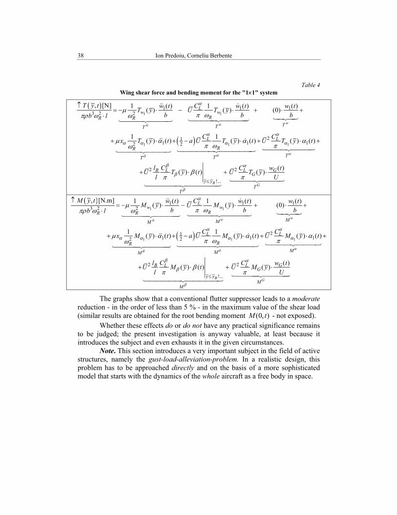
The corresponding formulae for shear and bending are set-up from the general expressions in Table 3, particularized for 1NW NA= = ; further, for direct use in the dynamic process, these must be expressed in physical time -see Table 4- in which the contributions of the various variables are explicitly identified. Notes 10. As expected, in the case of the controlled system, the wing loading "feels" the influence of the controller twice: through the wing dynamics ( ( ) , ( )w t tα ) itself and, directly, through the flap movement ( )tβ , both appearing in fact as response to the external gust perturbation. 20. The complete functions ( , )T y t and ( , )M y t are useful for the detailed wing design. Out of these, the value of the root shear, that is (0, )T t , is especially valuable since, in case of a free airplane, it determines the accelerations experienced by the fuselage itself (the technical application in this sense is the so-called "ride comfort control"…).

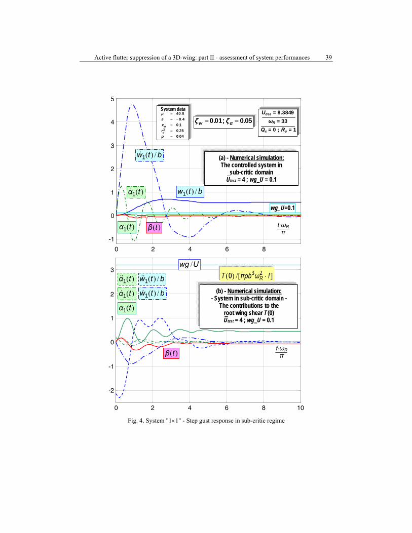
A) As a first numerical simulation, the dynamic response of the controlled system in the sub-critic domain has been established together with the corresponding wing root shear (0, )T t (Figure 4).

– The dynamic response is presented in Fig. 4-a, where, for clarity, all system variables have been individually displayed for comparison (note that the relatively high values of the time derivatives in comparison with the corresponding functions explain through the multiplicative effect of Rω !...).

– In an analogous manner, Figure 4-b shows the contributions to the shear force of various functions of time that build up its expression. In context, it must be observed that, since the accelerations do not appear in the state vector (14), they must be constructed numerically from these last…

B) In a second attempt, the direct effect of the controller on the wing loading has been investigated. Figure 5 presents the root shear force (0, )T t as it develops in time - as response to the same step gust - for the nominal and the controlled system, both in sub-critic regime.


Table 4 Wing shear force and bending moment for the "1×1" system

( )

( )

1 1

1 1 1

1 1 13 2 2

211 12 2

, [N] 1 ( ) 1 ( ) ( )( ) ( ) (0)

1 1( ) ( ) ( ) ( ) ( )

www

Lw w

RR RTTT

L L

RR

TT

T y t w t C w t w tT y U T yb b bb l

C Cx T y t a U T y t U T y

αα

α

α α

α α α α

μπ ωπρ ω ω

μ α α απ ω πω

↑= − ⋅ − ⋅ + ⋅ +

⋅

+ ⋅ + − ⋅ + ⋅ 1

2 2

!...

( )

( )( ) ( ) ( )B G

T

B L GLG

y yT

T

t

Cl C w tU T y t U T yl U

α

β

β α

β βπ π

≤

+

+ ⋅ + ⋅

( )

( )

1 1

1 1

1 1 13 2 2

211 12 2

, [N.m] 1 ( ) 1 ( ) ( )( ) ( ) (0)

1 1( ) ( ) ( ) ( )

www

Lw w

RR RMMM

L L

RR

MM

M y t w t C w t w tM y U M yb b bb l

C Cx M y t a U M y t U M

αα

α

α α

α α α α

μπ ωπρ ω ω

μ α απ ω πω

↑= − ⋅ − ⋅ + ⋅ +

⋅

+ ⋅ + − ⋅ +1 1

2 2

!...

( ) ( )

( )( ) ( ) ( )B G

M

B L GLG

y yM

M

y t

Cl C w tU M y t U M yl U

α

β

β α

β

α

βπ π

≤

⋅ +

+ ⋅ + ⋅

The graphs show that a conventional flutter suppressor leads to a moderate reduction - in the order of less than 5 % - in the maximum value of the shear load (similar results are obtained for the root bending moment (0, )M t - not exposed).

Whether these effects do or do not have any practical significance remains to be judged; the present investigation is anyway valuable, at least because it introduces the subject and even exhausts it in the given circumstances.

Note. This section introduces a very important subject in the field of active structures, namely the gust-load-alleviation-problem. In a realistic design, this problem has to be approached directly and on the basis of a more sophisticated model that starts with the dynamics of the whole aircraft as a free body in space.


0 2 4 6 8

-1

0

1

2

3

4

5

04025010

40040

2

.

.

...

===

−==

prxa

α

α

μ

Udes = 8.3849

ωR = 33

Qx = 0 ; Ru = 1 = =w αζ ζ. ; .0 01 0 05

( ) /1w t b

( ) /1w t b

( )1α t

( )1α t ( )β t

wg_U=0.1

(a) - Numerical simulation: The controlled system in

sub-critic domain Utest = 4 ; wg_U = 0.1

t·ωR π

0 2 4 6 8 10

-2

-1

0

1

2

3

t·ωR π

/wg U

( ) /1w t b( )1α t

( )1α t

( )β t

( ) /1w t b( )1α t(b) - Numerical simulation:

- System in sub-critic domain - The contributions to the

root wing shear T (0) Utest = 4 ; wg_U = 0.1

( ) /[ ]⋅RT πρb ω l3 20

System data

Fig. 4. System "1×1" - Step gust response in sub-critic regime


0 2 4 6 8 10

0.5

1.5

2

2.5

3

3.5

4

4.5 Max_T = 4.2112

t·ωR π

(a) - The nominal system

1

0 0 2 4 6 8 10

0

0.5

1

1.5

2

2.5

3

3.5

4

4.5

t·ωR π

Max_T = 4.1177

(b) - The controlled system

( ) /[ ]⋅RT πρb ω l3 20

Fig. 5. System "1×1" - Step gust response… - The root shear force (0, )T t

3. Conclusions and perspectives

The present article approaches a very actual and important aspect in the field of airplane design, namely the concept of active structures; out of this, the article concentrates on the active flutter suppression problem. Two are the major objectives of the proposed text:

To establish and numerically demonstrate a systematic methodology for the design of a flutter suppressor in case of a 3D-wing. The usefulness of a simplified model for preliminary design has been stated. For the design of the controller, the standard LQR algorithm has been used. As already said, the efficiency of this procedure has been validated experimentally by an extensive research program [2] which otherwise, as mentioned in Part I, established a national priority in the field of active structures.

To assess the efficiency of the flutter suppressor in sub-critic domain from a pure structural point of view. In this sense, the dynamic response of the controlled system under the action of a gust has been investigated. Explicit formulae for the wing internal loading and have been derived.

The numerical simulation performed on a test case demonstrates at least a moderate efficiency of the flutter suppressor as a gust-load-alleviator.

* Several continuations can be envisaged starting from this study from a

pure theoretical point of view (for instance the use of a more refined aerodynamic model - including numerical methods [3]) or from a practical perspective (for example the extension of the problem to the complete aircraft free in space).


w(y,t) EI , m

dm=m·dy

w

yO

y l

0 0.2 0.4 0.6 0.8 1-2

-1

0

1

2 Fw1Fw2 Fw3

η=y/ l

α(y,t) GId , J

dj=J·dy O

y l

y

-1

-0.5

0

0.5

1Fα1 Fα2Fα3

η=y/ l

0 0.2 0.4 0.6 0.8 1

4. Annex: The representation functions ( ) , ( )i jFw y F yα

The functions used in this text with the method of assumed modes are the free uncoupled vibration modes of a uniform cantilever beam. These can be found in any textbook on aeroelasticity and will be reproduced here for clarity (Fig. 6).

Fig. 6. Bending & Torsion vibration modes of the uniform beam

Bending. Differential equation: ( )'' " 0EI w mw⋅ + = , etc… – The modes are [4] (the first three displayed):

( )

( / )

sin sinh sinh sin cosh coscosh cos

i ii i i i i

i i

y l

N NFw N N N NN N

η

π π π η π η π η π ηπ π

=

⎡ ⎤⎛ ⎞−= − + −⎢ ⎥⎜ ⎟+⎝ ⎠⎣ ⎦

N1 = 0.596864… N2 = 1.494175… N3 = 2.500246… N4 = 3.499989… N5 = 4.500000… …

Torsion. Differential equation: ( )' ' 0GId Jα α⋅ − = , etc…

– The modes are (the first three displayed):

(2 1) ; sin(2 1) ( 1, 2,3, )2 2j j

GId yj F j nl J lπ πω α= − = − =

22

1 2(0.597) EIml

πω = 2

22 2(1.49) EI

mlπω = … ( )

2212 2i

EIiml

πω = −

(for i sufficiently high)


R E F E R E N C E S - See also Part I -

[1] I. Predoiu, C. Berbente, Active flutter suppression of a 3-D wing: Preliminary design and

Assessment (Part I: Problem statement & controller design), in UPB Sci Bull, Series D: Mechanical Engineering, ISSN 1454-2358, vol. 75, iss,2, 2013.

[2] I. Predoiu (Director de program), Studii teoretice şi experimentale privind amortizarea oscilaţiilor aeroelastice prin tehnici de control activ - Acronim AOCA, Contract de cercetare nr. 141/20.09.2004 (2004-2006) (Theoretical and Experimental Studies Referring to the Damping of the Aeroelastic Oscillations through Active Control Techniques - Research Program) - Agenţia Spaţială Română (Programul AEROSPAŢIAL) - Coordonator STRAERO Bucureşti, Subcontract de participare STRAERO-UPB(CCAS-Centrul de Cercetări pentru Aeronautică şi Spaţiu) (in Romanian).

[3] S. Dănăilă, C. Berbente, Metode numerice în dinamica fluidelor (Numerical Methods in Fluid Dynamics), Editura Academiei Române, Bucureşti, 2003 (in Romanian).

[4] W. Newsome Boyd, Effect of Chordwise Forces and Deformations and Deformations due to Steady Lift on Wing Flutter, PhD-Thesis, Stanford University, December 1977.

active flutter suppression of a 3d-wing: … · active flutter suppression of a 3d-wing:...

Documents