action recognition in depth videos using nonparametric … · action recognition in depth videos...
TRANSCRIPT

Action Recognition in Depth Videos using Nonparametric Probabilistic
Graphical Models
Natraj Raman
Submitted in partial fulfilment of the requirements for the degree of
Doctor of Philosophy
Department of Computer Science and Information Systems
Birkbeck, University of London
October, 2016

2
Abstract
Action recognition involves automatically labelling videos that contain human motion with
action classes. It has applications in diverse areas such as smart surveillance, human computer
interaction and content retrieval. The recent advent of depth sensing technology that produces
depth image sequences has offered opportunities to solve the challenging action recognition
problem. The depth images facilitate robust estimation of a human skeleton’s 3D joint positions
and a high level action can be inferred from a sequence of these joint positions.
A natural way to model a sequence of joint positions is to use a graphical model that describes
probabilistic dependencies between the observed joint positions and some hidden state
variables. A problem with these models is that the number of hidden states must be fixed a priori
even though for many applications this number is not known in advance. This thesis proposes
nonparametric variants of graphical models with the number of hidden states automatically
inferred from data. The inference is performed in a full Bayesian setting by using the Dirichlet
Process as a prior over the model’s infinite dimensional parameter space.
This thesis describes three original constructions of nonparametric graphical models that are
applied in the classification of actions in depth videos. Firstly, the action classes are represented
by a Hidden Markov Model (HMM) with an unbounded number of hidden states. The
formulation enables information sharing and discriminative learning of parameters. Secondly, a
hierarchical HMM with an unbounded number of actions and poses is used to represent
activities. The construction produces a simplified model for activity classification by using logistic
regression to capture the relationship between action states and activity labels. Finally, the
action classes are modelled by a Hidden Conditional Random Field (HCRF) with the number of
intermediate hidden states learned from data. Tractable inference procedures based on Markov
Chain Monte Carlo (MCMC) techniques are derived for all these constructions. Experiments with
multiple benchmark datasets confirm the efficacy of the proposed approaches for action
recognition.

3
Declaration
This thesis is the result of my own work, except where explicitly acknowledged in the text.
Copyright © 2016 Natraj Raman.
The copyright of this thesis rests with the author. No quotations from it should be published
without the author's prior written consent and information derived from it should be
acknowledged.

4
Publications
Portions of this thesis have been published.
[1] Raman, Natraj, Stephen J. Maybank, and Dell Zhang. "Action classification using a
discriminative non-parametric Hidden Markov Model." In International Conference on
Machine Vision (ICMV), London, UK, vol. 9067, p. 10, December 2013.
[2] Raman, Natraj, and Stephen J. Maybank. "Action classification using a discriminative
multilevel HDP-HMM." Neurocomputing (Journal), vol. 154, pp. 149-161, 2015.
[3] Raman, Natraj, and Stephen J. Maybank. "Activity recognition using a supervised non-
parametric hierarchical HMM." Neurocomputing (Journal), vol. 199, pp. 163-177, 2016.
[4] Raman, Natraj, and Stephen J. Maybank. "Non-parametric Hidden Conditional Random
Fields for Action Classification." In IEEE International Joint Conference on Neural
Networks (IJCNN), Vancouver, Canada, July 2016 (preprint).

5
Acknowledgements
I would like to express my sincere thanks to Prof. Steve Maybank for his insight, feedback and
support. Steve’s breadth and depth of knowledge is a huge inspiration and the opportunity to
study under his supervision was one of the main reasons I pursued a PhD course in Computer
Vision. Steve – the rigour and patience with which you review the works is unparalleled and I
am grateful for all your comments.
Thanks are also due to my second supervisor Dr. Dell Zhang for his comments and participation
in the review meetings. I thank Prof. Mark Nixon and Prof. Shaogang Gong for their suggestions.
Finally, I would like to thank my fellow PhD colleagues in the Birkbeck computer science
department who were a constant source of motivation.

6
Contents
1. Introduction .............................................................................................................. 14
1.1 Motivation ................................................................................................................... 14
1.2 Research Focus............................................................................................................ 16
1.2.1 Recognition from Joint Positions ........................................................................ 17
1.2.2 Challenges ........................................................................................................... 20
1.2.3 Graphical Models ................................................................................................ 20
1.3 Problem Definition ...................................................................................................... 22
1.4 Thesis Contributions ................................................................................................... 24
1.5 Thesis Structure .......................................................................................................... 26
2. Related Work............................................................................................................. 27
2.1 Overview ..................................................................................................................... 27
2.2 Features ...................................................................................................................... 28
2.2.1 Image Based Features ......................................................................................... 29
2.2.2 Skeleton Based Features ..................................................................................... 36
2.3 Classification ............................................................................................................... 40
2.3.1 Dimension Reduction .......................................................................................... 40
2.3.2 Static Classifiers ................................................................................................... 42
2.3.3 Dynamic Classifiers.............................................................................................. 43
2.4 Bayesian Nonparametric methods ............................................................................. 45
2.5 Summary ..................................................................................................................... 49
3. Background ............................................................................................................... 51
3.1 Hidden Markov Model ................................................................................................ 51
3.1.1 Inference ............................................................................................................. 53
3.2 Conditional Random Fields ......................................................................................... 54
3.3 Nonparametric Models ............................................................................................... 56
3.3.1 Dirichlet Process .................................................................................................. 57
3.3.2 Hierarchical Dirichlet Process ............................................................................. 61
4. Discriminative nonparametric HMM ........................................................................... 65
4.1 Overview ..................................................................................................................... 65
4.2 HDP-HMM ................................................................................................................... 68
4.3 Model .......................................................................................................................... 70
4.3.1 Two level HDP ..................................................................................................... 71
4.3.2 Transformed HDP Parameters ............................................................................ 72
4.3.3 Chinese Restaurant Process Metaphor ............................................................... 74
4.4 Discriminative Learning ............................................................................................... 75
4.4.1 Scaled HDP and Normalized Gamma Process ..................................................... 76

CONTENTS 7
4.4.2 Elliptical Slice Sampling ....................................................................................... 77
4.5 Posterior Inference ..................................................................................................... 78
4.5.1 Truncated Approximation ................................................................................... 78
4.5.2 Sampling State Transitions .................................................................................. 79
4.5.3 Sampling Component Parameters ...................................................................... 80
4.5.4 Prediction ............................................................................................................ 82
4.6 Experiments ................................................................................................................ 83
4.6.1 UTKinect-Action dataset ..................................................................................... 83
4.6.2 MSR Action 3D dataset ....................................................................................... 90
4.7 Conclusion ................................................................................................................... 96
5. Supervised nonparametric Hierarchical HMM ............................................................. 98
5.1 Overview ..................................................................................................................... 98
5.2 Hierarchical HMM ..................................................................................................... 101
5.3 Activity Model ........................................................................................................... 104
5.3.1 Structure ........................................................................................................... 104
5.3.2 Generative Process ........................................................................................... 106
5.4 Posterior Inference ................................................................................................... 108
5.4.1 Sampling Hidden State Sequence ..................................................................... 108
5.4.2 Sampling Parameters ........................................................................................ 112
5.4.3 Prediction .......................................................................................................... 113
5.5 Experiments .............................................................................................................. 114
5.5.1 Cornell Activity Dataset ..................................................................................... 114
5.5.2 HDM05 Dataset ................................................................................................. 124
5.6 Conclusion ................................................................................................................. 127
6. Nonparametric HCRF ............................................................................................... 128
6.1 Overview ................................................................................................................... 128
6.2 Parametric HCRF ....................................................................................................... 131
6.3 Model ........................................................................................................................ 132
6.3.1 Parameters ........................................................................................................ 132
6.3.2 Bayesian Extension............................................................................................ 134
6.3.3 Nonparametric HCRF ........................................................................................ 135
6.4 Posterior Inference ................................................................................................... 137
6.4.1 Hidden state sequence sampling ...................................................................... 138
6.4.2 Sampling parameters ........................................................................................ 138
6.4.3 Sampling scale variables ................................................................................... 139
6.4.4 Prediction .......................................................................................................... 139
6.5 Experiments .............................................................................................................. 140
6.6 Conclusion ................................................................................................................. 147
7. Conclusions ............................................................................................................. 148

CONTENTS 8
7.1 Summary ................................................................................................................... 148
7.2 Limitations................................................................................................................. 150
7.3 Future Research ........................................................................................................ 151
7.4 Final Remarks ............................................................................................................ 153
A. Active 3D Sensors .................................................................................................... 154
A.1 Structured Light Imaging ........................................................................................... 154
A.2 Time-of-flight Imaging ............................................................................................... 157
B. Pose Estimation ....................................................................................................... 159
C. Bayesian Approach .................................................................................................. 162
C.1 Probability Model ...................................................................................................... 162
C.2 Posterior Analysis ...................................................................................................... 164
C.3 Conjugate Priors ........................................................................................................ 165
D. Graphical Models ..................................................................................................... 168
D.1 Bayesian and Markov networks ................................................................................ 168
D.2 Sequential Data Modelling ........................................................................................ 171
D.3 Message Passing ....................................................................................................... 172
E. Approximate Inference ............................................................................................ 175
E.1 Simulation Methods .................................................................................................. 175
E.2 Gibbs Sampling .......................................................................................................... 176
E.3 Slice Sampling ........................................................................................................... 178
References ...................................................................................................................... 180

9
List of Figures
1.1 Applications of automatic event recognition. .................................................................. 15
1.2 Biological motion perception. .......................................................................................... 17
1.3 The Kinect sensor.. ........................................................................................................... 19
1.4 Joint positions estimation.. .............................................................................................. 19
1.5 Sequential data in a graphical model.. ............................................................................. 21
1.6 Clustering and Dirichlet processes.. ................................................................................. 23
2.1 Features types.. ................................................................................................................ 29
2.2 Holistic representations.. ................................................................................................. 31
2.3 Local representations.. ..................................................................................................... 33
2.4 Skeleton data features.. ................................................................................................... 37
2.5 Classification algorithm types........................................................................................... 41
3.1 HMM representation.. ...................................................................................................... 52
3.2 Viterbi decoding.. ............................................................................................................. 54
3.3 Linear Chain CRF.. ............................................................................................................. 56
3.4 Chinese Restaurant Process.. ........................................................................................... 59
3.5 Dirichlet Process.. ............................................................................................................. 60
3.6 Chinese Restaurant Franchise.. ........................................................................................ 62
3.7 Hierarchical Dirichlet Process.. ......................................................................................... 64
4.1 Discriminative HDP-HMM overview.. ............................................................................... 67
4.2 Graphical representation of HDP-HMM.. ......................................................................... 69
4.3 Graphical representation of the two level HDP-HMM.. ................................................... 73
4.4 UTKinect-Action dataset samples.. ................................................................................... 83
4.5 Skeleton Hierarchy.. ......................................................................................................... 85
4.6 Hidden states plot. ........................................................................................................... 87
4.7 UTKinect-Action dataset results.. ..................................................................................... 90
4.8 MSR Action3D dataset samples.. ...................................................................................... 91
4.9 Feature descriptor visualization.. ..................................................................................... 91
4.10 Action states.. ................................................................................................................... 94
4.11 MSR Action 3D dataset results.. ....................................................................................... 96
5.1 Activity Recognition Overview.. ..................................................................................... 100
5.2 Graphical representation of a Hierarchical HMM. ......................................................... 102
5.3 Graphical representation of the activity Model.. ........................................................... 105
5.4 Cornell-Activity dataset samples.. .................................................................................. 115

LIST OF FIGURES 10
5.5 Learned hierarchical structure for the rinsing mouth activity. ...................................... 118
5.6 Action states for the activities involved in the kitchen location.. .................................. 119
5.7 Cornell Activity dataset - Confusion matrix. ................................................................... 123
5.8 Motion capture system.. ................................................................................................ 125
5.9 HDM05 dataset samples.. .............................................................................................. 125
5.10 Pose clustering.. ............................................................................................................. 126
6.1 Graphical representation of a HCRF. .............................................................................. 131
6.2 Graphical representation of a Bayesian nonparametric HCRF. ...................................... 136
6.3 KARD dataset samples. ................................................................................................... 141
6.4 Hidden state instantiation. ............................................................................................. 142
6.5 Histogram plot of the parameter values in a posterior sample. .................................... 143
6.6 KARD dataset classification results.. ............................................................................... 145
A.1 Structured Light Imaging.. .............................................................................................. 155
A.2 Depth computation in Kinect.. ....................................................................................... 156
A.3 Time-of-flight principle. .................................................................................................. 157
B.1 Pose estimation pipeline.. .............................................................................................. 161
C.1 Gaussian density plots.. .................................................................................................. 163
C.2 Dirichlet distribution plots.............................................................................................. 166
D.1 Graphs showing the relationships between random variables. .................................... 169
D.2 Markov assumption. ...................................................................................................... 172
D.3 Message Passing.. .......................................................................................................... 174
E.1 Slice Sampling. ................................................................................................................ 179

11
List of Tables
4.1 Posterior Inference Algorithm ........................................................................................... 82
4.2 Classical Parametric HMM classification results ............................................................... 86
4.3 HDP-HMM classification results ........................................................................................ 86
4.4 Multi-level HDP-HMM classification results ...................................................................... 88
4.5 Summary of classification results for the UTKinect-Action dataset. ................................. 89
4.6 Actions organized into three different action sets in the MSR Action3D dataset. ........... 92
4.7 Summary of classification results for the MSR Action 3D dataset. ................................... 96
5.1 Posterior Inference Algorithm ......................................................................................... 113
5.2 Cornell activity dataset - Classical Parametric HMM classification accuracy .................. 120
5.3 Cornell activity dataset - Parametric H-HMM classification accuracy ............................ 121
5.4 Cornell activity dataset - Classification accuracy ............................................................ 121
5.5 Cornell activity dataset - Classification accuracy (in %) for the full model. .................... 122
5.6 Summary of classification results for Cornell Activity dataset. ....................................... 123
5.7 Summary of classification results for HDM05 dataset. ................................................... 125
6.1 Posterior Inference Algorithm ......................................................................................... 139
6.2 The three different action sets in the KARD dataset. ...................................................... 142
6.3 Summary of classification results for the KARD dataset. ................................................ 145
6.4 Cornell activity dataset - Classification accuracy. ........................................................... 146
E.1 Gibbs Sampling Algorithm ............................................................................................... 176

12
Notational Conventions
General
ℝ The set of real numbers
ℤ+ The set of positive integers
𝕀(𝑎 = 𝑏) An indicator function that evaluates to 1 if 𝑎 = 𝑏, 0 otherwise
𝑥𝑛 The 𝑛𝑡ℎ training example sequence
𝑦𝑛 The class that the 𝑛𝑡ℎ training example belongs to
𝑥𝑡 Observation at time instant 𝑡
𝑧𝑡 Hidden state at time instant 𝑡
휃 Set of all model parameters
HDP-HMM
𝛽𝑘 Probability of transitioning to state 𝑘
𝜋𝑗𝑘 Probability of transitioning to state 𝑘 given state 𝑗
𝛾 Dirichlet Process hyper parameter for 𝛽
𝛼 Dirichlet Process hyper parameter for 𝜋
𝜇𝑘 , Σ𝑘 Mean and covariance of Gaussian distribution corresponding to component 𝑘
𝜇0, Σ0 Gaussian distribution hyper parameters for 𝜇
𝜈0, Δ0 Inverse Wishart distribution hyper parameters for Σ
Chapter 4
𝜑𝑗𝑘𝑐 Probability of transitioning to state 𝑘 given state 𝑗 for class 𝑐
𝜆 Dirichlet Process hyper parameter for 𝜑
𝜌𝑘𝑐 Parameter for shifting mean 𝜇𝑘 for class 𝑐
Λ𝑘𝑐 Parameter for scaling covariance Σ𝑘 for class 𝑐
𝜔𝑗𝑘𝑐 Parameter used for scaling 𝜑𝑗𝑘
𝑐 for class c
Ω0 Hyper parameter for 𝜌
𝜗0, 𝜎0 Hyper parameters for Λ
휀0 Hyper parameter for 𝜔
휃𝑐 Set of model parameters for class 𝑐
휃\𝑐 Set of model parameters excluding class 𝑐
휃𝑠 Set of model parameters shared for all the classes
𝐿 Upper bound on the number of HMM states
𝜉0 Prior controlling importance of discriminative term
휁0 Prior controlling the distance between distributions
Chapter 5
𝑎𝑡 Action state at time instant 𝑡
𝑎 Empirical frequencies of the action states
𝒂 Action state sequence from a sampling iteration
𝜌𝑘𝑎 Probability of transitioning to pose state 𝑘 given action 𝑎
𝜑𝑗𝑘𝑎 Probability of transitioning to pose state 𝑘 given state 𝑗, action 𝑎
𝑓𝑡 Binary variable indicating whether a sequence of actions is complete
𝜓 Probabilities of completion for action state
𝜚 Dirichlet Process hyper parameter for 𝜌
𝜏 Dirichlet Process hyper parameter for 𝜑
𝜅𝑎, 𝜅𝑏 Hyper parameters for 𝜓
휂 Regression coefficients
𝜆 Hyper parameter for the regression coefficients
𝐾𝑎 Upper bound on the number of action states
𝐾𝑠 Upper bound on the number of skeleton states

NOTATIONAL CONVENTIONS 13
𝐾𝑜 Upper bound on the number of object states
𝑉(. ) Forward message value
𝑚(. ) Backward message value
Chapter 6
𝑍 Normalization constant
𝜓 Potential function
𝜑𝐿𝐵𝐿 Feature function for dependency between a hidden state and a label
𝜑𝑇𝑅𝑁 Feature function for dependency between two hidden states and a label
𝜑𝑂𝐵𝑆 Feature function for observations dependency
휃𝐿𝐵𝐿 Parameter group corresponding to 𝜑𝐿𝐵𝐿
휃𝑇𝑅𝑁 Parameter group corresponding to 𝜑𝑇𝑅𝑁
휃𝑂𝐵𝑆 Parameter group corresponding to 𝜑𝑂𝐵𝑆
𝜎2 Global scale
𝜙 The scale variable with exponential distribution prior
𝜼 The set of scale variables with the HDP prior
휂𝐿𝐵𝐿 The scale variables corresponding to 휃𝐿𝐵𝐿
휂𝑇𝑅𝑁 The scale variables corresponding to 휃𝑇𝑅𝑁
휂𝑂𝐵𝑆 The scale variables corresponding to 휃𝑂𝐵𝑆
𝜅 Dirichlet Process hyper parameter for 휂

14
1. Introduction
The topic of this thesis is introduced in this chapter. It begins with the motivation for action
recognition in Section 1.1. This is followed with a discussion on the use of depth images and
graphical models in Section 1.2. The specific problems that this thesis investigates are described
in Section 1.3. The main contributions of this thesis are listed in Section 1.4 and finally the thesis
structure is outlined in Section 1.5.
1.1 Motivation
Videos provide visualization of complex and dynamic situations in an intuitive manner. They are
a popular medium to convey information. The rate at which video data are generated has
increased very rapidly of late due to the ubiquitous availability of devices that record videos.
There are an estimated 50 million hours of footage generated every day by the surveillance
cameras in the U.K. [57] and about 400 hours of video is uploaded every minute into the popular
YouTube website [56]. With the advent of future developments in wearable devices, the amount
of video content will increase even further. It is difficult to interact with such enormous amounts
of video data without efficient tools that automatically describe, organize and manage them.
In order to effectively describe the content in a video, the objects and events occurring in the
image sequences that comprise the video must be detected and recognized. State-of-the-art
tools in computer vision provide the ability to detect and recognize the objects and their
properties in images [59, 60]. However, robust and accurate recognition of events that occur in
image sequences is still a problem. This is unsurprising since the cognitive underpinnings for
understanding events are much more complicated. It requires application of complex
spatiotemporal concepts. The research here addresses this challenging computer vision problem
and provides mechanisms to recognize events involving humans in videos.
Automatic human event recognition has many applications across various domains (Figure 1.1).
For example, in the security domain, there is an ever increasing need to monitor video feeds for
interesting events. These video feeds may originate from CCTV cameras or from other
sophisticated platforms used by the military such as unmanned aerial and ground vehicles. The
current monitoring solution involves dedicated human operators actively watching live video
streams. This is often undesirable since the human operators are expensive resources and it is
difficult for them to remain focused at all times. Instead, an automated system that can detect

CHAPTER 1 - INTRODUCTION 15
and recognize interesting events and then alert the human operators is required. Such a system
is cost-effective and eliminates potential security risks.
Figure 1.1: Applications of automatic event recognition. (a) A smart surveillance system that
detects interesting events in live video feeds [60]. (b) Monitoring the daily living activities in a
care centre [61]. (c) Analysing an American football sports video for offensive team formation
[3]. (d) Natural user interaction with a games console for a better gaming experience [62]. (e)
Touchless interaction for browsing and manipulating medical images during surgery in an
operating theatre [2].
Smart surveillance systems that discard routine events and highlight only interesting events
have applications in other domains such as healthcare. For example, in a care centre for the
elderly, the automatic recognition of an inmate’s irregular sleep patterns, changes in the
(d) (e)
#ALERT: DROPPED-ITEM
(a)
(b) (c)

CHAPTER 1 - INTRODUCTION 16
frequency of toilet use and difficulties in performing regular activities helps in assessing the
cognitive and physical well-being of the person [63]. Health monitoring surveillance systems can
reduce expenses and improve the quality of life for the elderly.
Multimedia information retrieval is another important area where automatic event recognition
is essential. A content based search and retrieval system would enable the efficient explorations
of large volumes of archived video data. As example use-cases, a user may wish to view all
archived videos that contain a wedding event or a security professional may wish to review
frames that contain an explosion event in surveillance footages. The current technique for
searching the videos is limited to metadata queries and text search based on manual
annotations. Instead, searching directly for user-defined events provides a comprehensive
mechanism to interact with the video content. With automatic event recognition, the videos can
be indexed analogously to text document indexing and abstracts such as key frames or highlights
can be extracted to form condensed summaries of the videos. In effect, the videos can be
managed as structured artefacts and analysis can be performed on their contents [1]. Content
based search, retrieval and analysis of videos have applications in innumerable areas including
sports, education and arts.
The pervasive use of computing has encouraged researchers to explore more natural and
intuitive mechanisms to interact with computers. In addition to voice and hand gestures, the
use of the entire human body to communicate with computers has gained traction of late. For
example, the Microsoft Xbox game consoles allow players to interact through their full body
without the need for a games controller [62]. The player can perform actions such as kick or
jump to naturally convey their intended motion to the console. This provides an immersive
gaming experience for the player. In order to respond to player movements the console must
detect and recognize the various events that occur during the interaction. The applications for
such natural ways of interacting are not restricted to entertainment platforms. They can also be
used in many other scenarios such as medical surgery. A surgeon can control and manipulate
equipment without explicit contact, thus maintaining the boundaries between sterile and non-
sterile parts of the surgical environment [2].
The above wide range of applications in diverse areas such as smart surveillance, content
retrieval and human computer interaction provides a motivation for addressing the human
event recognition problem.
1.2 Research Focus
The term “event” can refer to a variety of concepts at different levels of abstraction and at
different time scales, ranging from elementary movements of a body part by an individual to

CHAPTER 1 - INTRODUCTION 17
complex interactions between persons that can last for hours. In order to distinguish between
the different types of events, a standard terminology [4] is followed. An elementary motion such
as raising a leg is referred to as a “gesture”. The composition of multiple elementary motions,
carried out by a single person and organized temporally is referred to as an “action”. Walking
and sitting down are examples of actions. The term “pose” refers to a particular configuration
of the human body that is encountered while performing an action. Hence gestures and actions
can alternatively be described by sequences of poses. An “activity” is composed of a set of
actions that occur over time. For example the activity rinsing the mouth may contain drink and
spit actions. This thesis focuses exclusively on action recognition for videos that involve a single
individual and last less than a minute.
1.2.1 Recognition from Joint Positions
The famous Johansson experiments [12], illustrated in Figure 1.2, demonstrate that motion can
be perceived from sparse visual input. It was shown that moving light displays attached to a
small number of landmark joints on the human body provide sufficient motion cues to infer
actions such as walking, running etc. The visual system can detect motion patterns by integrating
the movements of individual joints over space and time. The absence of shape, colour and
texture information does not inhibit the recognition of the motion. The use of a handful of body
joints to model articulated human motion produces a compact representation for the human
actions. Hence determining the locations of the joints corresponding to the various body parts
and modelling the spatiotemporal transitions of these joint positions provides the necessary
information to characterize motion and infer actions and activities.
Figure 1.2: Biological motion perception. Point lights are placed on joint locations. When a
sequence of these point lights is viewed, the actions walk and run are apparent even though the
figure outline is omitted [12, 13].
Recovering the body joints from images is a very difficult problem because there is a
fundamental loss of information when a 3D scene is projected into a 2D image. It is often not
possible to robustly identify the body parts in an image. The pixels in an image typically encode

CHAPTER 1 - INTRODUCTION 18
intensity variations as RGB colour values. Different lighting conditions induce variations in the
recorded pixel values. Human body parts in an image might be partially occluded by other
objects or by the parts themselves from time to time. The image may contain shadows. Further,
background clutter may make it difficult to locate the objects of interest and perspective
deformations can make it difficult to recognize the objects. Even though the RGB videos contain
rich visual information, their sensitivity to lighting conditions and the difficulty in performing
robust background subtraction in these videos pose significant challenges for estimating
articulated human body motion [6, 142].
A depth image, which contains information relating the distance of an object in a scene to a
camera, is less affected by the above image representation issues. The depth images are robust
to colour and texture variability induced by clothing, hair and skin of a human body. It is much
easier to detect the human body silhouette using depth information rather than RGB values. The
3D data that includes depth information simplifies background subtraction, resolves silhouette
ambiguities and is largely invariant to lighting, colour and texture [7, 9].
The traditional way to obtain 3D data is stereo vision [8] in which the depth information is
reconstructed by capturing 2D images from multiple viewpoints. Unfortunately, the inference
of depth information involves complex stereo geometry calculations and is affected by
reflections, depth discontinuities and sparse textures in the images. Stereo vision suffers from
the same lighting and segmentation problems associated with colour images. The need for
multiple synchronized cameras and the unreliable depth information produced by an expensive
reconstruction process limits the applications of stereo vision [5]. An alternative is to use motion
capture systems [86] in which special markers are attached to the body and the 3D joint
positions are obtained by triangulation using multiple cameras. Even though this procedure
provides accurate body motion, its intrusive nature is infeasible in real world scenarios and the
high cost of the hardware restricts its application to niche areas.
Recent advances in depth sensing technology have provided cameras that produce synchronized
colour and depth images. The Microsoft Kinect sensor [10] contains an infrared projector, an
infrared camera and a colour camera. It produces reasonably accurate depth images in addition
to the RGB images at high frame rates. The distance of the 3D points in the world from the image
plane is recorded as pixel values in the depth image as shown in Figure 1.3. Note that the sensor
can provide depth information only up to a limited distance and the depth estimates are
sometimes inaccurate. Further, the captured structure is pseudo 3D because the points that are
not in front of the sensor cannot be recorded. In spite of these limitations, the low-cost and
relatively small footprint of these sensors make them a popular choice for recording depth
images.

CHAPTER 1 - INTRODUCTION 19
Figure 1.3: The Kinect sensor. The RGB image is produced by a RGB camera and the depth
image is produced by an infrared projector and an infrared camera. The points close to the camera
have darker pixel values. The black pixels indicate that depth values are not available for those
pixels [10, 11].
The detection of joint positions is greatly simplified by the use of depth images. The pioneering
work in [14] introduced a mechanism to robustly classify the depth image pixels associated with
a human body, by assigning to them an appropriate body part label. The locations of the joints
can then be estimated from these pixel labels. An overview of this approach is provided in Figure
1.4. The algorithm is computationally efficient and is built into the Kinect sensor so that the joint
positions are provided in real-time.
Figure 1.4: Joint positions estimation. An intermediate labelled image in which each pixel is
classified into a body part is inferred from the depth image. The 3D joint positions are estimated
from the labelled image [14, 9].
RGB Camera RGB Image
Depth Image Infrared Projector Infrared Camera
Depth image Body part labels Joint positions

CHAPTER 1 - INTRODUCTION 20
Inspired by the Johansson experiments and the recent breakthrough in depth sensing
technology, the research in this thesis uses the locations of joints estimated from depth images
to characterize the motion patterns. The action classes are modelled using sequences of these
joint positions.
1.2.2 Challenges
Even with the availability of body joint positions, recognizing actions is not that simple. There
exists similarities in different action classes and there are often differences within the same class
of actions. For example, walk and run actions involve similar sets of joints. The movements for
a walk action can differ in speed and style between individuals. As the number of action classes
increase, the overlap between them will be higher, making it much harder to distinguish
between actions of different classes. The actions are also of varying duration with sequences of
different lengths. This makes them difficult to compare.
The joints information may be corrupted by noise due to inaccurate depth estimates. It may also
be necessary to change the coordinate system of the positions to account for differences in
recording environment and variations in size and shape between humans. In many cases, the
joints space is of high dimension containing redundant information and it is important to find
compressed representations to facilitate computationally inexpensive comparisons between
the actions.
The need to generalize over large intra-class variations and maximize small inter-class
distinctions, along with the need to handle temporal variations and noisy sequences make action
recognition intrinsically challenging. Application of advanced statistical machine learning
techniques is required to address this problem.
1.2.3 Graphical Models
Action recognition is usually regarded as a supervised classification problem [35]. Prototypical
examples of videos and their corresponding action class labels are made available for training.
The prediction of action class labels for new unseen videos is based on the information learned
during training. What distinguishes action classification from traditional supervised
classification is that an input observation is a sequence of data points that are strongly
correlated over time. In effect, action classification is a sequence labelling problem in which each
sequence of data is assigned a sequence of class labels.
A natural way to model the sequential data is to introduce a discrete valued state variable that
compactly represents the observed data at a time instant. These state variables can then be
reasoned about, as they evolve over time. The discrete valued state at a particular time is a
snapshot of the relevant attributes of the observed data at that time [15]. As an example, in a

CHAPTER 1 - INTRODUCTION 21
clap action, the various intermediate body poses such as hands together, hands apart etc. may
correspond to different state variables and by examining the transitions between these state
variables (i.e. body poses), an action is inferred. Since these states are not explicitly observed in
the input data, they are often referred as hidden states or latent states.
Figure 1.5: Sequential data in a graphical model. The state variables S describe the observations
O𝑡 at various time instants 1, 2, … , T, T+1 etc. The dependency relations between the variables
are expressed in a graph structure. The states are conditioned only on the previous state and not
on the entire history.
It is essential to perform a probabilistic reasoning over these state variables to account for
uncertainties in the outcomes. For a probabilistic formulation, a joint distribution over the space
of possible states must be constructed. It is daunting to represent these distributions over many
variables naively. A diagrammatic representation provides mechanisms to visualize the structure
in these complex distributions and exploit them. Probabilistic graphical models use a graph
based representation to simplify dependencies over many variables to a smaller subset of
variables. The nodes in the graph correspond to the variables and the graph edges express the
dependency relationship between these variables.
It is impractical to assume that the future states depend on all previous states. Such an
assumption leads to an intractable model that grows with the number of observations. A
reasonable approximation would be to consider that the past is independent of the future given
the present. This Markov assumption shown in Figure 1.5, together with the assumption that all
the data are generated from the same distribution, allows the modelling of sequential data in a
compact form [16].
The Hidden Markov Model (HMM) [32] is a well-known graphical model that is used to represent
sequential data. An HMM uses a set of discrete states and a state is conditioned only on the
state at a previous time instant. The Conditional Random Field (CRF) [33] is another probabilistic
S1
S2
ST
...
O1 O
2
OT
...
ST+1
OT+1
...
...

CHAPTER 1 - INTRODUCTION 22
model that uses a graph based representation to encode relations between states at different
time instants. While the HMMs use directed graphs, the CRFs use undirected graphs.
The research in this thesis uses discrete state-space graphical models such as HMM and CRF to
deal with the dynamics regulating the temporal evolution of the body joints. The graph based
declarative structure provides a flexible framework for encoding complex interactions between
many variables. Further, it also enables the development of a generic solution with the
representation and inference procedures applicable to problems in many other domains.
1.3 Problem Definition
A general problem with the graphical models that use discrete state variables is that the number
of hidden states must be fixed a priori. This number is not known in advance for most
applications. Let us the take the example of the action class models described above in which
the state variables represent the various body poses. A prior knowledge of the exact number of
intermediate poses that are involved when performing an action is not available. The motion
patterns and body positions may vary subtly between two subjects who perform the same action
and consequently the number of poses may depend on the number of subjects. Further, these
numbers must be specified separately for every action since almost certainly the number of
poses will differ between actions depending on their complexity. If a large number of states is
specified, it may result in a complex model that over fits the data and fails to fit new
observations. A small number of states may not be adequate to capture the variations in the
data.
The classical solution for this problem is to perform model selection – several models are fit to
the data and then one of the models is selected using a model comparison metric. In the above
problem, typically several models are trained with different numbers of states and a procedure
such as cross-validation or regularization is used to choose a model with the correct number of
states. In cross-validation, the model is evaluated on small subsets of the training data to see
how well it generalizes and in regularization a penalty term that favours a simpler model is
incorporated during training [17].
Unfortunately such procedures do not adapt well to changes in data complexity. Instead of these
ad-hoc procedures that compare multiple models which vary in complexity, it is preferable to fit
a single model that estimates the number of states automatically from data. Such a mechanism
avoids any misfit between the number of states and the amount of training data. The model
complexity, as measured by the number of states, increases as the amount of data increases.
However, the formulation of a model with an unbounded complexity is nontrivial. The set of all
possible solutions must be considered and the parameter space is now infinite dimensional.

CHAPTER 1 - INTRODUCTION 23
A model over an infinite dimensional parameter space can be defined using Bayesian
nonparametric methods [18, 73]. These methods employ an unbounded number of parameters
but only a small subset of these parameters are actually used. Appropriate prior distributions
control the number of parameters required to model the data. Small datasets produce simple
models while complex datasets induce rich models, thereby adapting the effective model
complexity to the data. The lack of an upper bound on the number of parameters mitigates
under-fitting while the computation of a posterior distribution of the parameters in a Bayesian
approach reduces the chance of over-fitting.
Figure 1.6: Clustering and Dirichlet processes. The data points are generated from a mixture of
2D Gaussians with 50 data points in the left, 150 data points in the middle and 500 data points in
the right. The clusters learned through Dirichlet Process are shown as ellipses. The number of
clusters increase with the number of data points.
The Dirichlet process [19] is one of the most popular priors employed in Bayesian nonparametric
methods. It is a distribution over distributions i.e. a sample drawn randomly from a Dirichlet
process is itself a probability distribution. A common application of Dirichlet process is as a prior
distribution in mixture models used for clustering data. In mixture models, each data point is
assumed to belong to a cluster, with the data points inside a cluster distributed randomly within
that cluster. The number of clusters must be specified a priori in classical clustering techniques.
The use of a Dirichlet process prior instead provides a mechanism that estimates both the
number of clusters and the parameters of the distributions characterizing the clusters
simultaneously from data. An unbounded number of clusters is available, but only a small
number of them are used to model a given set of data points. Large clusters grow larger, faster.
When the number of data points increases, new clusters may emerge as illustrated in Figure 1.6.
This nonparametric solution is evidently better at dealing with the combinatorial challenge
associated with model selection procedures.
Although the use of Dirichlet Process as a nonparametric prior for graphical models was explored
before [40, 41, 44] these techniques by themselves are unsuitable for a supervised classification

CHAPTER 1 - INTRODUCTION 24
problem. A straight forward application of these techniques would use a separate model to
represent each action class and define a joint distribution over the input observations and the
class label. Such generative models describe the input while in a classification problem the
objective is to discriminate between the inputs. Formulating models such that they provide the
best decision boundaries to distinguish the classes is necessary. Furthermore, the use of
separate models prohibits the sharing of valuable information across the different action
classes. Information exchange between classes is essential to facilitate effective learning with a
small number of training examples. It is important to consider a nonparametric prior that is
suitable for classification tasks.
The central computation problem in Bayesian nonparametric methods is posterior inference –
i.e. estimating the posterior distribution of the model parameters given the observed data. The
posterior distribution often has a highly complex form. Except in the simplest cases, there are
no closed form expressions readily available to evaluate the posteriors analytically. The use of
sequential data compounds the problem. When deriving inference algorithms, it is important to
consider multiple variables together and make large moves in the probability space for
computational efficiency.
The research presented in this thesis deals with the important problem of choosing models at
an appropriate level of complexity and ensuring that these models are suitable for supervised
classification. It investigates the following research questions in the context of action
recognition:
Question 1. How to represent actions and activities using graphical models?
Question 2. How to learn the number of states in the graphical models from data rather than
using model selection procedures?
Question 3. How to share information between the action classes?
Question 4. How to ensure that the models are discriminative in nature so that the best decision
boundaries to distinguish the actions can be found?
Question 5. How to perform efficient posterior inference over the model parameters?
1.4 Thesis Contributions
Motivated by the lack of existing methods to address the above questions, this thesis proposes
three different and original constructions of nonparametric graphical models that are suitable
for action classification.

CHAPTER 1 - INTRODUCTION 25
The actions are represented using the Hidden Markov Model (HMM) [32] and Hidden
Conditional Random Field (HCRF) [95], two well-studied discrete state-space graphical models
used widely in sequential pattern recognition. The activities contain an inherent hierarchical
structure and they are represented using a Hierarchical Hidden Markov Model (H-HMM) [81].
All the three models use 3D joint positions obtained from depth video to define the features. In
the attempt to answer Question 2, nonparametric variants of the canonical HMM, H-HMM and
HCRF are developed. This avoids ad-hoc model selection procedures and flexibly adapts the state
cardinality to changes in data. Further, the model parameters are formulated in terms of
distributions that are common across the classes to facilitate information sharing. To address
the fourth question, the models are constructed in such a way that they are suitable for
supervised classification problems. Finally, posterior inference procedures that are efficient for
sequential data are derived for all the models based on simulation [36] techniques. The main
contributions are summarized as follows:
A discriminative nonparametric HMM for action classification
The classical HMM is extended with a nonparametric prior and augmented with a discriminative
term. The resulting model infers the number of hidden states automatically, with the model
parameters learnt in a manner that is suitable for classification tasks. The model formulation
promotes effective transfer of information between action classes. The model is evaluated for
action classification on benchmark depth video datasets containing locations of joints.
A supervised nonparametric H-HMM for activity classification
A hierarchical extension to the HMM with an unbounded number of action and pose states is
developed. The formulation uses multinomial logistic regression to distinguish between the
activity classes based on action states, thereby simplifying the model structure. The model
efficacy is demonstrated for activity classification with joint positions and depth information
used to characterize activities.
A nonparametric HCRF for action classification
A nonparametric extension to the HCRF that precludes the need to specify the number of
intermediate hidden states is proposed. The discriminative HCRF models the classification rules
directly. The Bayesian treatment of the training procedure provides realistic characterization of
uncertainty in the parameters. Good classification results are achieved in two different depth
video datasets containing human actions.
The proposed models are applicable to a wide variety of sequence labelling problems, besides
action sequences. The investigations in this thesis have been published in [192, 193, 194, 195].

CHAPTER 1 - INTRODUCTION 26
1.5 Thesis Structure
These contributions are discussed in greater detail in the subsequent chapters of this thesis. A
brief description of the remaining chapters is as follows:
Chapter 2 reviews a broad range of works that are related to this thesis. The approaches used
for vision based human action recognition in the literature are surveyed. The various features
extracted from the depth images are discussed in detail. The different classification techniques
are outlined. A review of the nonparametric solutions used in the literature and how they
compare with the work in this thesis is also included.
Chapter 3 provides the technical background necessary to describe the models used in this
thesis. The HMM and CRF models are introduced. The Dirichlet process, which is extensively
used as a nonparametric prior in subsequent chapters, is described. Further background
information including the techniques used to construct depth images and the statistical
framework upon which the action class models are built is provided in the Appendix.
Chapter 4 presents an action classification technique using a discriminative nonparametric
HMM. The action classes are represented by a multi-level Hierarchical Dirichlet Process (HDP)
HMM. The model parameters are formulated as transformations from a base distribution and
are learnt in a discriminative manner. The chapter begins with the motivation for this approach,
presents the model and derives the posterior inference mechanism. Finally the experiments
section discusses the results obtained on two different datasets.
Chapter 5 develops a two level hierarchical HMM to perform activity classification. The bottom
level states characterize granular poses while the top level states characterize the coarser
actions associated with activities. In order to perform classification, the relationship between
the actions and activities are captured using multinomial logistic regression. The chapter begins
with an overview of the approach, provides the activity model structure and explains the
inference mechanism. The evaluations conducted on two different datasets are also discussed.
Chapter 6 proposes the use of a HCRF for classifying actions. The classical HCRF is extended with
a nonparametric structure and the number of hidden states is automatically inferred. The
training and inference procedures are fully Bayesian. The construction is based on scale mixtures
of Gaussians as priors over the HCRF parameters and uses the slice sampling technique during
inference. The model representation and the mechanism to perform Bayesian inference are
presented along with the experiments.
Chapter 7 concludes the thesis by summarizing the main contributions. Several future directions
and perspectives of the proposed techniques are presented.

27
2. Related Work
The aim in vision based action recognition is to determine the action type of a previously unseen
video. It is an active research area and the vast amount of papers published in the literature
every year related to this topic is a testimony to both its importance and the challenges involved.
This chapter reviews the existing literature on action recognition. Over the years many
techniques have been proposed. The focus in the review here is mainly on the approaches to
recognition based on depth images and a graphical model based representation.
The approaches differ mainly in the features and the classification algorithms that are used. The
various feature descriptors extracted from the image sequences are discussed in Section 2.2.
The different classification techniques, ranging from those that explicitly model the temporal
dynamics of the motion to those that do not, are covered in Section 2.3. The Bayesian
nonparametric framework is used in the recognition procedure presented in this thesis. Section
2.4 surveys the various nonparametric approaches. A final summary is provided in Section 2.5.
This chapter provides insight into how the thesis differs from the other related work.
2.1 Overview
The research efforts in vision based action recognition date back as far as the early 1990s when
Yamato et al. [104] used Hidden Markov Models to classify tennis strokes. Some of the early
methods used for motion analysis are reviewed in [105]. A variety of approaches have been
proposed since then and there are several surveys in the literature that provide an overview of
these methods. Some of the surveys are discussed below.
The techniques used for tracking, pose estimation and recognition are surveyed in [106]. The
review presented in [107] expands the recognition scope to include methods used for
interpreting cognitively higher level activities. The survey in [55] covers the various features
that are extracted from the image sequences for action classification. In [4], a comprehensive
summary of the approaches used for activity analysis is presented using a tree structured
taxonomy. Yet another survey [108] lists the methods used for representing, segmenting and
learning actions. The recent survey in [110] discusses the state-of-the-art research using the
taxonomy defined in [4]. A survey of the datasets available for human action recognition is
presented in [109].

CHAPTER 2 – RELATED WORK 28
The above surveys deal mainly with action recognition using visible light colour images. With the
widespread availability of low-cost depth sensors, there has been lot of research interest of late
in using the depth image sequences for human motion analysis. There are a few survey papers
that review approaches based on 3D data in the context of action recognition. The surveys in [6]
and [111] discuss depth data acquisition and the pre-processing steps involved. In addition, they
review the algorithms used for action analysis. The other surveys that focus on human action
recognition with 3D data include [5, 112, 113] and the very recent [114].
Most action recognition methods assume that some examples of videos and their corresponding
action class labels are available. A typical system first defines an abstract and compact
representation of the patterns in a video, commonly referred as features. A model is then
learned for the action classes during a training process using the features extracted from the
example videos. Given a video whose action label is not known, this video is matched against
the learned model in order to classify it. The variations in recognition methods are mainly based
on the features and the classification algorithms used for matching the features.
2.2 Features
This section discusses the methods used to determine an image sequence representation that
is suitable for robust classification of the actions. It is important to choose informative and
discriminative features. This process, known as feature extraction, is treated as the core problem
in many action recognition works. Off-the-shelf classifiers are often used for matching the
features once they are obtained.
It is crucial to capture the temporal correlations between the images in the video for successful
recognition. Some methods extract the features frame by frame and convert the video into a
sequence of feature vectors. The matching algorithm used during classification analyses this
sequence to deduce the action. In other methods, the features explicitly include temporal
information.
While the range of features used for action recognition can seem overwhelming, the majority of
them can be divided broadly into two categories: image based and skeleton based. In the latter,
an explicit model of the human body is defined and pose estimation is performed on the images
to determine the configuration of the body. This provides the skeleton – a schematic
representation of the locations of the body parts. The features are then chosen from the
positions of the joints that are part of the skeleton. In contrast, image based methods avoid
reconstructing the human form and rely on extracting features directly from the images in a
video. It is not usual to define an intermediate body model or explicitly identify the body parts.

CHAPTER 2 – RELATED WORK 29
The two categories are discussed in detail below with an emphasis on the features used for
action recognition in depth images. Figure 2.1 lists the feature types discussed in this review.
2.2.1 Image Based Features
A diverse palette of low-level visual features has been proposed for action recognition. The
image based features fall under two types – those in which the features are encoded from the
human as a whole and those that use a collection of local descriptors obtained from several
image patches. Some methods use both types of feature. A pose estimation procedure is
typically not performed when computing image based features. These features can be extracted
even from images in which the resolution is low.
Figure 2.1: Features types. The various features used for action recognition are shown in a
schematic representation. See text for more details.
Holistic Representations
The holistic representations consider the image region of interest in full. They often follow a top
down approach, first detecting and extracting the human being before computing the features.
The actions are characterized using the appearance and motion information obtained from the
localized human. These methods are generally sensitive to noise and are affected by variations
in viewpoint and occlusion [55]. However, they have been used successfully in many action
recognition works both for colour and depth videos.
Features
Image Based
Holistic Representations
Silhouettes
Contours
Optical Flow
Local Representations
Interest Points
Feature Descriptors
Skeleton Based
Relative Joint Positions
Joint Angles
Histograms
Joint Selection

CHAPTER 2 – RELATED WORK 30
The human silhouette, in effect the foreground of a person in an image, provides a simple
representation that carries useful shape information about the body pose. The evolution of the
silhouettes over time can be used to recognize the actions. Instead of taking into account all the
pixels within a silhouette, sometimes only the boundary pixels are used. These boundary points,
which contain no information about the internal structure of the image, have also been used to
approximate the body poses.
An early work using silhouettes is [115], where the differences between binary silhouettes are
accumulated to construct a Motion Energy Image (MEI) and a Motion History Image (MHI). The
former indicates where motion has occurred while the latter indicates how the motion evolves
in the temporal domain. The MEI and MHI together define an action template and recognition
is performed by matching these templates based on a statistical model of the moments. The
work in [116] employed an extended Radon transform on the binary silhouette to define
features that are invariant to geometrical transformations such as scaling and translation. The
actions are regarded as 3D shapes induced by stacking the 2D silhouettes in the space-time
volume in [117]. The space-time shapes (Figure 2.2 (a)) encode both the spatial information of
the body and the global body motion. The extremities of a human body such as head, hands and
feet are used in a representation of the body posture in [118]. These extremities are detected
from a body contour. In [119], the contours of the MEI are used to obtain a contour coded MEI
that is invariant to scale changes and translations.
It is not always easy to obtain stable shape information from colour images. The robustness of
the extracted silhouettes and contours relies heavily on how accurate the background
subtraction is. When compared with the colour images, it is much easier to perform background
subtraction in depth images. Hence the silhouettes extracted from depth images are usually
noise free. The above silhouette based features have been extended successfully from the 2D
colour images to the 3D depth images for action recognition.
In [120], the MHI is extended to include the depth information. The resulting three dimensional
motion history image (3D-MHI) augments the conventional MHI with additional channels that
encode the motion history in the depth changing directions. The pixel values in the 3D-MHI
include a history of the increase and decrease in depth values. An activity recognition system for
smart homes is developed in [121] using depth silhouettes. The extended Radon transform
employed for the binary silhouette in [116] is extended here to the depth silhouettes. The
ambiguity for different poses is more pronounced among the binary silhouettes, while the depth
silhouettes, with a richer set of intensity values, provide a better mechanism to differentiate
between the poses.
CHAPTER 2 – RELATED WORK 31
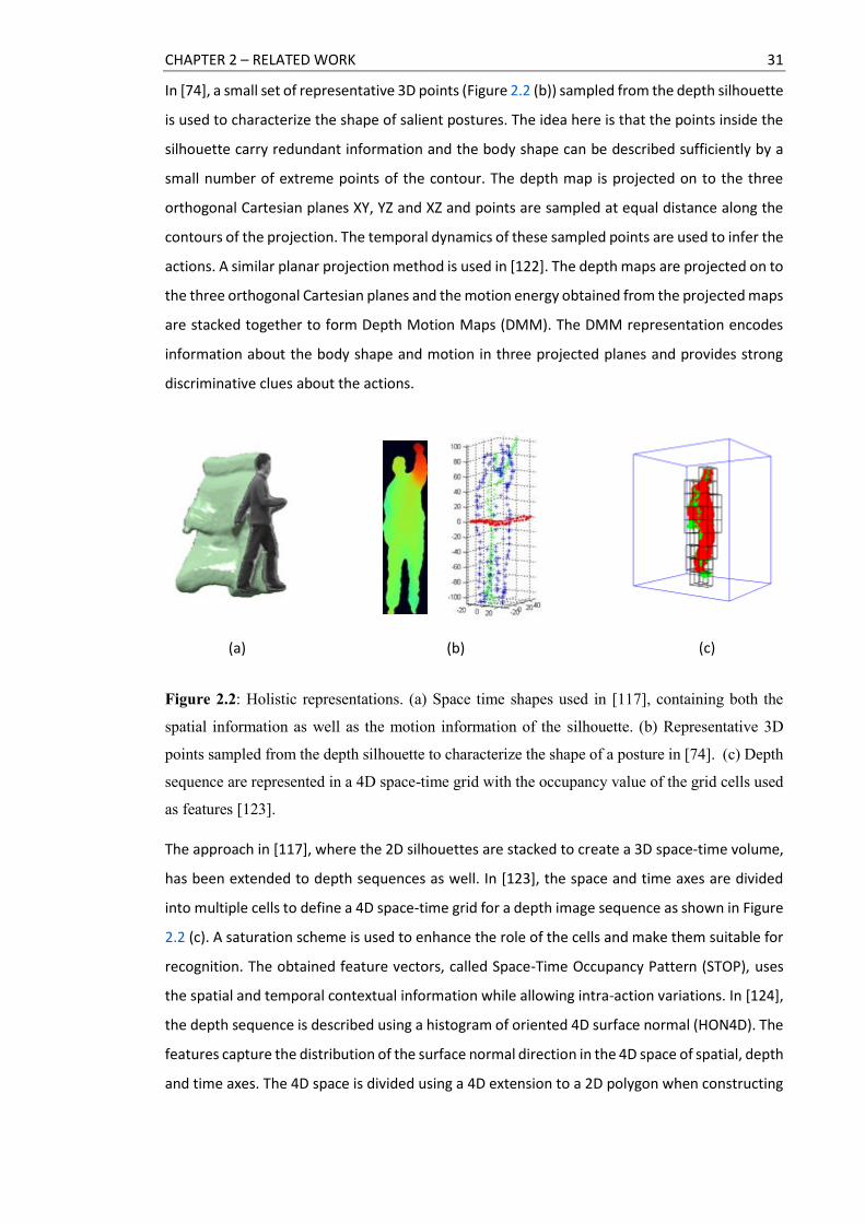
In [74], a small set of representative 3D points (Figure 2.2 (b)) sampled from the depth silhouette
is used to characterize the shape of salient postures. The idea here is that the points inside the
silhouette carry redundant information and the body shape can be described sufficiently by a
small number of extreme points of the contour. The depth map is projected on to the three
orthogonal Cartesian planes XY, YZ and XZ and points are sampled at equal distance along the
contours of the projection. The temporal dynamics of these sampled points are used to infer the
actions. A similar planar projection method is used in [122]. The depth maps are projected on to
the three orthogonal Cartesian planes and the motion energy obtained from the projected maps
are stacked together to form Depth Motion Maps (DMM). The DMM representation encodes
information about the body shape and motion in three projected planes and provides strong
discriminative clues about the actions.
Figure 2.2: Holistic representations. (a) Space time shapes used in [117], containing both the
spatial information as well as the motion information of the silhouette. (b) Representative 3D
points sampled from the depth silhouette to characterize the shape of a posture in [74]. (c) Depth
sequence are represented in a 4D space-time grid with the occupancy value of the grid cells used
as features [123].
The approach in [117], where the 2D silhouettes are stacked to create a 3D space-time volume,
has been extended to depth sequences as well. In [123], the space and time axes are divided
into multiple cells to define a 4D space-time grid for a depth image sequence as shown in Figure
2.2 (c). A saturation scheme is used to enhance the role of the cells and make them suitable for
recognition. The obtained feature vectors, called Space-Time Occupancy Pattern (STOP), uses
the spatial and temporal contextual information while allowing intra-action variations. In [124],
the depth sequence is described using a histogram of oriented 4D surface normal (HON4D). The
features capture the distribution of the surface normal direction in the 4D space of spatial, depth
and time axes. The 4D space is divided using a 4D extension to a 2D polygon when constructing
(a) (b) (c)

CHAPTER 2 – RELATED WORK 32
the features. It is argued that the distribution of the normal vectors for each cell in the 4D space
contains more information than the occupancy patterns.
In addition to the shape based features, optical flow based features have also been used. The
pixel wise oriented differences between frames are captured and used to estimate the optical
flow in the image regions undergoing change. Optical flow based features are particularly
applicable in the cases where background subtraction is difficult and the image resolution is
poor. However they may fail when there are sudden changes in motion.
In [125], actions are recognized based on optical flow measurements obtained from sports
footage in a setting where the image of a whole person may only be 30 pixels are so tall. The
pixel-wise optical flow captures motion independent of appearance. Since the optical flow
computation is inaccurate in noisy data, the optical flow vectors are treated as a spatial pattern
of noisy measurements. The optical flow is used to extract person-centric motion features in
[126] for recognizing actions such as biking, diving etc. in colour videos. In order to allow for the
noise in the optical flow, a windowing scheme is used here.
The application of optical flow to depth images for action recognition was explored in [127]. The
optical flow is computed as an extension to the third dimension of the traditional 2D optical
flow. However, the computation is restricted to some portions of the 3D scene. A grid based
descriptor is used for representing the flow information extracted from the point cloud within a
temporal sequence. The extraction of optical flow from depth data has been limited. The main
challenge is that the computation of optical flow on all the 3D points in a scene is prohibitively
expensive.
Local Representations
A collection of features extracted from independent image patches are used in the local
representations. These local features effectively capture the shape and motion information in
the video. These methods follow a bottom-up approach. First a set of interest points are
identified and then the features are extracted from local patches around these interest points.
The features from multiple patches are combined together to obtain a final representation.
Unlike the holistic representations, detecting the humans and performing background
subtraction may not be necessary with this approach. Hence these methods are suitable even
in the situations where action recognition must be performed in unconstrained poor quality
videos. The methods are generally less sensitive to noise than holistic representations and may
be invariant to rotation and scale. However, it is often computationally expensive to construct
the features based on local representations.

CHAPTER 2 – RELATED WORK 33
The interest points such as corners and edges contain significant local variations of the image
intensities and carry information that is stable under small perturbations. They are well studied
in the spatial domain and have been applied to many object recognition tasks in static images.
The notion of spatial interest point is extended to the temporal domain in [128] by requiring the
image values in the spatiotemporal volumes to have significant variations along both the spatial
and temporal directions. These spatiotemporal interest points (STIPs), shown in Figure 2.3 (a),
correspond to image points that have large image intensity variations and non-constant motion.
The features obtained by generalizing the Harris corner detector to the spatiotemporal domain
are used in [128] to identify interesting events in image sequences.
Figure 2.3: Local representations. (a) Spatiotemporal interest points detected in [128] during a
walking action. (b) Interest points detected from a depth image sequence for the drink action in
[137]. (c) The numbers of points that fall into the cells of a localized spatial grid are used in [88].
There are other extensions of the 2D spatial interest point detection mechanisms to the 3D
space-time axes for action recognition. In [129], the image sequences are represented using a
collection of points that are salient both in space and time. The 2D saliency metric is based on
measuring the changes in the information content of a circular image region over a set of
different scales. This is extended to the temporal domain by considering cylindrical
neighbourhoods at different scales and temporal depths. The obtained points using the 3D
saliency detector correspond to activity variation peaks. A 3D Discrete Wavelet Transform
(DWT) is used in [130] to detect spatiotemporal salient regions. The image sequences are
represented in a 3D Euclidean space with time as the third dimension. A multiscale 3D DWT is
applied to decompose the 3D volume and the resulting coefficients are used to compute
saliency. The actions are represented using simple features of the salient regions. The interest
point detector in [135] uses a Gabor filter on the temporal domain. At each interest point, a
cuboid that contains the spatiotemporally windowed pixel values is extracted to determine the
feature vectors. The detector errs on the side of detecting too many interest points rather than
(a) (b) (c)
CHAPTER 2 – RELATED WORK 34
too few. This is motivated by the observation that irrelevant features generated by scene clutter
are handled well in object recognition tasks.
While the interest point detector selects locations and scales, the feature descriptors capture
shape and motion information in the neighbourhoods of selected points using image gradients.
They encode statistics of the pixel distributions. Similar to the extension of interest point
detectors from the spatial domain to the spatiotemporal domain, the feature descriptors have
also been extended to the spatiotemporal domain and have been applied to action recognition.
The well-known Histogram of Oriented Gradients (HOG) descriptor [77] used for detecting
humans in static images is generalized in [131] to the 3D spatiotemporal domain. The orientation
of the spatiotemporal gradients is quantized using a polyhedron and the gradient histograms of
all the 3D cells are concatenated and normalized. The resulting HOG3D descriptor is used to
recognize actions. A similar extension is proposed in [132] to compute histogram descriptors of
space-time volumes in the neighbourhood of interest points. The resulting descriptor is used to
recognize human actions that occur in movie videos.
The local representations based on the spatiotemporal interest points and feature descriptors
originally developed for colour images have been extended to depth videos. In [136], a 4-
dimensional local spatiotemporal feature that combines both colour and depth information is
used for activity recognition. This work is inspired by the local features developed for colour
videos in [135]. It uses separate response functions along the spatial and temporal dimensions
to detect the interest points. The features are obtained by computing the colour and depth
gradients from a 4D hyper cuboid centred at the interest point. The work in [137] detects
interest points in the depth image (Figure 2.3 (b)) using the same technique proposed in [135]
for visible light images. An additional function is employed for correcting the noise encountered
in the depth maps, for example holes and value jumps. A 3D cuboid which contains the
spatiotemporally windowed pixel values around the interest points is used to define a
descriptor. The various interest point detectors and feature descriptors used for depth images
are evaluated in [134]. They include the Harris3D [128] and Cuboid [135] interest point detectors
extended for the depth images. The feature descriptors include HOG3D [131], HOG/HOF [132]
and HOG [77].
New types of feature descriptors that are motivated directly by action recognition in depth
images have also been explored. In [138], a descriptor called Histogram of Oriented Principal
Components (HOPC) is proposed to capture the local geometric characteristics around each
point within a sequence of 3D point clouds. In order to obtain the descriptor at a point, first
Principal Component Analysis (PCA) is performed on a spatiotemporal volume around the point.
The resulting Eigenvectors are projected onto a number of directions corresponding to the

CHAPTER 2 – RELATED WORK 35
vertices of a polyhedron and are scaled by the Eigenvalues. The descriptor formed by
concatenating these projected Eigenvectors is used when performing action recognition. The
HOPC descriptor is claimed to be invariant to changes in viewpoints. In [139], a descriptor called
Local Depth Pattern (LDP) is obtained by computing the average depth values in a spatial cell
that is constructed from the interest points identified in a colour image. The Comparative Coding
Descriptor (CCD) used for action representation in [140] encodes the structural relations of
points in space and time. The video is treated as a spatiotemporal volume of depth values and
a set of small atomic cuboids extracted from this volume is used to construct a sequence of
codes that define the descriptor. The CCD has some invariance to perspective variations and
sufficiently depicts the depth information necessary for action recognition.
The occupancy patterns of the 3D spatial point cloud used in the holistic representations are
also applicable as local representations. The numbers of points that fall into the cells of a
localized spatial grid (Figure 2.3 (c)) are used as features in [88]. These Local Occupancy Pattern
(LOP) features describe the appearance in a sub region of the depth image and are useful in
characterizing the interactions with objects when an action is performed. A set of features called
Random Occupancy Pattern (ROP) is proposed in [141] for recognizing actions. The depth
sequence is considered as a 4D spatiotemporal volume in which the pixel values are binary. The
ROP features are defined by the sum of the pixel values in a sub-volume. There are a number of
sub-volumes with different sizes and at different locations. Since the possible set of sub-volumes
is prohibitively large, a random sampling approach is used to efficiently explore the sub-
volumes.
The methods that rely exclusively on image based features for action recognition in depth videos
are becoming less popular. The estimation of human body poses in real time has become
possible with the use of depth images as demonstrated in [14]. The low-level visual features are
less important when pose information is available. The locations of the various body joints
provide essential information to discriminate between the actions. However, using image based
features in conjunction with the pose information may be effective in some recognition
scenarios.
The action recognition methods in this thesis are based on the pose information. Hence the
above techniques where the features are extracted directly from the depth images are not
applicable on this work. A notable exception is in Chapter 5 where a hybrid of the pose
information and depth channel is used. The information in the depth image patches is used to
characterize the objects a person performing an activity interacts with and some of the feature
descriptors discussed above are employed in that chapter.

CHAPTER 2 – RELATED WORK 36
2.2.2 Skeleton Based Features
A number of approaches for action recognition, including those in this thesis, are motivated by
the seminal study [12] of motion perception by Johansson, in which it was demonstrated that
actions can be understood just from a small number of landmark joints. A hierarchy of joints
connected by bones forms a skeleton and different joint configurations yield different poses.
The actions can now be described using a sequence of positions of these joints in the skeleton
rather than by the pixel values in an image.
The human body is capable of a wide range of motions and estimating the configuration of the
human body from a sequence of monocular images is non-trivial. It is difficult to compensate
the loss of depth information that results from the formation of a 2D image. As alluded to in
Chapter 1, the variations in appearance, colour, texture and lighting further compound the
problem. Despite several years of research [55, 58], pose estimation from visible light images
remains largely unsolved [142].
The introduction of depth sensors provided a realistic opportunity to infer the body poses. In
particular, it was demonstrated in [14] that pose estimation can be performed in real time if
depth images are used. The algorithm proposed in [14] powered the commercially available
Kinect sensor, which produces estimates of a skeleton structure that is composed of 20 joints.
This algorithm is discussed in Appendix B, but in a nutshell, first a depth image is segmented
probabilistically into body parts and then proposals of 3D body joint positions are generated
from this intermediate segmented image.
The availability of 3D joint positions aroused considerable interest in the action recognition
community and several works were published using the skeleton information. However,
recognition is still a challenge even when using body joint positions. The variations within the
same action class, similarities in motion patterns between the action classes and noisy skeletons
due to sensor errors, occlusions etc. make it difficult to distinguish between the actions robustly.
This necessitates further processing of the joint positions to derive alternative feature
representations [114].
A simple feature for representing human motion is the pairwise relative position where the
difference between the 3D positions of any two joints is used. The intuition behind this feature
is that an action can be described in terms of the relations between any two body parts. For
example, a “wave” action can be described as “hands” above “shoulder” and “wrists” to the left
or right of “elbow”. In [88] the feature for a joint is determined by taking the difference between
the position of a joint and all the other joints. The overall feature is determined by enumerating

CHAPTER 2 – RELATED WORK 37
all the pairwise joints. A similar mechanism is employed in [89] to determine a dynamic skeleton
(DS) feature using relative joint positions.
Figure 2.4: Skeleton data features. (a) Spherical coordinate system in [11] that uses the hip centre
joints for aligning the coordinates with a person’s direction. The angles are divided into equal
sized bins to derive a histogram based representation. (b) Joint angles representation used in [149].
(c) A local skeleton descriptor that encodes the relative positions of joint quadruples is used in
[156].
In [147], the relative joint positions computed from several video frames are used as features.
Apart from the differences between the joints in the current frame, the pairwise differences are
computed between the current frame and a preceding frame to capture the motion properties.
The pairwise differences are also computed between the current frame and an initial frame that
approximates the neutral posture. The combination of all these differences forms a feature
representation. Instead of using the difference between two joints, the distance between two
joints is used in [148]. The Euclidean distances between every pair of points in the current frame
and previous frames are used in the feature representation. The Euclidean distances between
all pairs of joints in the current and adjacent frames are also used in [159] to determine the
features. This work additionally includes as features the velocity of a joint along the direction
defined by two other joints and the velocity of a joint in the direction of the normal vector of
the plane spanned by three other joints.
(a) (b)
(c)

CHAPTER 2 – RELATED WORK 38
Instead of using the 3D joint positions, some action recognition methods use the joint angles as
features. In a kinematic tree representation of the human body [142], a particular joint is
selected as the root and the remaining joints are connected to the root in a hierarchical manner.
A set of relative joint angles that represent the orientation of the body parts with respect to the
parent in the hierarchy provides an alternative representation of the 3D locations of the joints.
The 3D Cartesian coordinates representing the joint positions are transformed into 2D spherical
angles representing the directions of the body parts. The radial distance is omitted in the
representation thus excluding the length of the body parts. This angular skeleton representation
provides some invariance to the size of the human and the orientation of the depth sensor.
In [80], the relative azimuth and elevation angles of each joint with respect to its parent in the
skeleton hierarchy are used to compute the features. For example, in order to calculate the
feature at the left elbow joint, first the sensor coordinate system at this joint is translated such
that the origin is at the left shoulder. Then a local spherical coordinate system is constructed in
terms of an elevation angle from the XY plane and an azimuth angle from the positive X axis. A
spherical coordinate system is also used in [11] to derive view invariant features. The hip centre
joint is defined as the centre of the spherical coordinates and the spherical coordinates are
aligned with the direction of a person (Figure 2.4 (a)). The angles between the limbs and the
angles between limbs and planes spanned by the body parts are used in [151]. The works in
[152, 153, 154] also employ joint angles as features for action recognition with [154] using
quaternions for representing rotations.
A similar joint angle representation is used in [149] with each joint position represented using a
pair of azimuth and elevation angles that specify the joints in a locally defined spherical
coordinate system. However, the angles are computed a little differently. The positions
corresponding to the joints at neck, shoulder, spine and hips are considered as points of a torso
that is a vertically elongated rigid body as shown in Figure 2.4 (b). An orthonormal basis is first
obtained from these points and the other joints are represented relative to this basis. The joints
adjacent to the torso such as elbows, knees and head are called first-degree joints and are
represented relative to the adjacent joint in the torso in a spherical coordinate system derived
from the torso frame. The same torso frame is used as a reference to convert the second-degree
joints such as the hands and feet at the extremities. A problem with this method is that it may
produce inconsistent angles and non-local descriptions for the second-degree joints. This
method is improved in [150] by considering rotations of the torso orthonormal basis when
constructing the angles for the second-degree joints.
Instead of using the joint positions or the joint angles, some methods propose representations
that explicitly model the geometric relationships among the body parts. In the recent work [155],

CHAPTER 2 – RELATED WORK 39
the 3D geometric relationships between various body parts are described using rigid body
transformations. A family of relative 3D geometry-based skeletal representations, referred as
R3DG features, is introduced. In [156], a skeleton descriptor that encodes the relative positions
of a set of four joints (Figure 2.4 (c)) is proposed. Given a quadruple of nearby joints, a coordinate
system such that one of the joint position is the origin and one of them is mapped to [1,1,1] is
considered. A similarity transformation is applied on the remaining two joints with the
quadruple encoded by six parameters that are well distributed in a 6D space.
Instead of directly using the joint positions or the joint angles as features, some methods apply
further processing on these to derive sophisticated feature descriptors. For example, in [11] the
azimuth and elevation angles of the hip centre joint are divided into equal sized bins as shown
in Figure 2.4 (a) and the angles corresponding to the other joints are probabilistically assigned
to the bins. The final descriptor called Histogram of Oriented Joints 3D (HOJ3D) is computed
from the histogram bins. In [157], a histogram of the directions between joints in the current
frame and adjacent frames is used. The resulting descriptor called Histogram of Oriented
Displacements (HOD) represents the motion of an object based on the distance it moves. In
[160], the spherical coordinates of the joint positions are quantized into a histogram with an
action modelled as a set of histograms. The number of bins is different for the azimuth and
elevation angles. The covariance matrix of the joint positions is used to derive a Covariance of
3D Joints (Cov3DJ) descriptor in [158].
Some methods hypothesize that not all the joints contain useful information for action
recognition and a feature selection step is introduced to identify a subset of joints that are more
helpful in discriminating the actions. This may be done manually using some a-priori knowledge
on the data. For example in [152], a specific set of 8 joints are identified to recognize activities
related to falling event. The joints on the limbs are excluded since they are perceived to
introduce more noise than useful information required to decide whether a person has fallen.
Similarly in [11], 12 joints are pre-selected manually before constructing the features. The
excluded joints either contain redundant information or do not contribute to distinguishing the
motions.
Instead of manual selection, in some methods the joints are selected automatically when
constructing the features. For example, in [153] the most informative joints in a time window
are identified based on the relative informativeness of all the joints in that time window. The
joints that have high variance of their angular changes are defined as the most informative
joints. In [160], a pose feature is defined as a weighted sum of all the joint features with the
weights learned using a Partial Least Squares (PLS) method. A Support Vector Machine (SVM)
model is trained in [88] to determine how discriminative the features extracted from a joint are.

CHAPTER 2 – RELATED WORK 40
This information is used to find the features for a subset of the joints. Even evolutionary
computation methods such as Genetic Algorithm (GA) have been used to identify a subset of
joints in the skeleton hierarchy that provides a good representation of the motion patterns
[161].
Skeleton based features are used in the action recognition methods in this thesis. The simple
pairwise relative positions of the joints are mainly used as features. More sophisticated
descriptors are avoided. The temporal dynamics of the joints, as modelled by the classification
algorithm, are relied upon to distinguish the actions. The classification algorithms proposed in
this thesis are generally agnostic to the features and are designed to benefit from other types
of sequential data.
2.3 Classification
While the previous section discussed the methods used to extract features from the video, this
section describes the methods used to match the features. Once the features are available, the
action recognition problem becomes a supervised classification problem. A variety of algorithms
in statistical machine learning literature can be used to match the features. The classification
algorithms used for action recognition can be divided broadly into two types – static and
dynamic. In the static classifiers, the temporal domain is not considered while in the dynamic
classifiers the variations of the features in time are explicitly modelled. Figure 2.5 lists the
classification algorithm types discussed in this review.
2.3.1 Dimension Reduction
Before using the classification algorithms, many action recognition methods apply a dimension
reduction technique. The features extracted from the video frequently contain redundant
information, may be sparse vectors and are sometimes noisy. They are often in a very high
dimensional space, for which a large number of training examples is required. Using a
compressed form of the features hugely benefits the classification algorithm. Hence the features
are subjected to a dimension reduction technique to obtain a robust and compact
representation.
The Principal Component Analysis (PCA) [16] is a commonly used linear dimension reduction
method which projects high dimensional features to a lower dimensional feature space. It is
employed in various works such as [123, 136, 147] to reduce the number of features. Linear
Discriminant Analysis (LDA) [35], which preserves the class discriminatory information while
reducing the dimensions, is used in [11] and [121]. In [88], a short Fourier transform is applied
to the feature vector at a time instant and the low frequency Fourier coefficients are used as

CHAPTER 2 – RELATED WORK 41
features. By discarding the high frequency Fourier coefficients the features are made robust to
noise.
Figure 2.5: Classification algorithm types. The classification algorithms used for action
recognition are shown in a schematic representation. Some methods optionally include a
dimension reduction step and use code words. See text for more details.
Non-linear dimension reduction methods have also been explored for action recognition. These
techniques, known as manifold learning, identify the underlying low dimensional manifold in
which the high dimensional features are embedded in such a way that the properties of the
original feature space are preserved. The assumption here is that by the nature of the human
movements, the actions do not span the entire feature space and hence they must lie on a low
dimensional manifold. The features obtained as a result of manifold learning are used by the
classifier.
In [162], a low dimensional embedding of the actions is learnt from the high dimensional
trajectories of the joints using a manifold functional variant of PCA. In [79], the trajectories
described by the 3D joint positions are embedded in a Riemannian manifold. This formulation
takes advantage of the Riemannian geometry in the resulting shape space when comparing the
similarities between the shapes of different trajectories. The intuition behind this approach is
that the feature descriptors used in vision applications typically lie on a curved space due to the
Classification
Static Classifiers
k-NN
SVM
Dynamic Classifiers
HMM
H-HMM
DBN
CRF
Dimension Reduction
Vector Quantization
CHAPTER 2 – RELATED WORK 42
geometric nature of their definitions. Another recent work [163] uses an autoregressive moving
average (ARMA) model, which is parameterized using an observability matrix, to represent the
trajectory of the joint positions. The subspace spanned by the columns of the observability
matrix corresponds to a point on a Grassmann manifold.
2.3.2 Static Classifiers
When static classifiers are used for action recognition, it is assumed that the feature
representation already captures the information in the temporal dimension. Typically, the entire
video is summarized by a single feature vector. This may result in feature vectors of different
sizes because the number of frames in a video may vary between the actions.
Many methods such as [131, 134, 152] etc. use a bag-of-features or bag-of-words model in which
the features are represented using a fixed size histogram. Typically a clustering algorithm such
as K-means is applied to the feature vectors to learn a set of centroid vectors called the code
words. Each feature vector is mapped to a code word by the index of its closest centroid. A set
of feature vectors can now be represented by the histogram of the code words. This method of
quantizing the feature vector is often employed to produce a global feature representation of
the entire action sequence when static classifiers are used. The loss of temporal structure with
this quantization does not matter since the static classifiers do not model the time dimension
anyway.
The 𝑘-Nearest Neighbour (𝑘-NN) classifier compares the distance between the feature vector of
a test video and the feature vectors of the videos in the training examples to determine the class
label. The label most common among the 𝑘 closest training examples in the feature space is
chosen. The 𝑘-NN classifier has been used for classifying actions in many methods such as [79,
115, 117, 119, 125, 127, 129, 147]. Different distance measures have been used. For example,
the Euclidean distance is used in [117], Mahalanobis distance is used in [115], the Chamfer
distance is used in [129], the geodesic distance is used in [79] and a video to class distance based
on naïve Bayes is used in [147]. It is also possible to use a distance measure in 𝑘-NN that
compares two feature sequences, possibly of different lengths. For example, in [154], the
Dynamic Time Warping (DTW) algorithm is used as a distance measure.
The 𝑘-NN classifier scales well with the number of classes and also avoids the over fitting
problem. It also does not generally need a training procedure. However, a stored database of
previously seen actions is necessary with this classifier. If there are a number of training
examples, comparisons become computationally expensive. Hence an adequately
representative set of training examples must be identified with this classification method.

CHAPTER 2 – RELATED WORK 43
One of the most popular static classifiers for action recognition is the Support Vector Machine
(SVM) [65]. This discriminative classifier, which learns a hyperplane in the feature space that
separates the classes, has been used by several methods such as [122, 124, 131, 132, 134, 137,
139, 140, 141, 152 157]. Both linear SVMs (e.g. [157]) and non-linear SVMs, (e.g. [134]) in which
the inputs are mapped to a high dimensional feature space using kernel functions such as chi-
squared kernel, have been used. The probabilistic variant of the SVM, the Relevant Vector
Machine (RVM) has also been used for action recognition in [129].
The use of SVM as off-the-shelf classifier by many methods is unsurprising since it has produced
stellar results for many other computer vision problems such as object recognition and human
detection [77]. However, since SVMs cannot model temporal data the classifier performance
depends on how well the features capture the time dimension.
2.3.3 Dynamic Classifiers
Unlike static classifiers that consider a single data point, the dynamic classifiers analyse a
sequence of data points. The temporal dynamics are explicitly modelled in the dynamic classifier
and the order of the features are considered when matching them. Sequential patterns of data
are observed in many other fields such as speech recognition (e.g. phoneme sequences),
genomics (e.g. DNA sequences) and natural language processing (e.g. sentences). There is a rich
body of literature on sequential pattern recognition. This survey focuses on those methods that
use a state-space graphical model for action recognition. See [4, 107, 114] for other approaches.
In most state-space graphical models, discrete valued state variables are encoded as graph
nodes. The edges between the states and the observed features characterize the model. The
most well-known model in this family is the Hidden Markov Model (HMM) [32]. The sequence
of states in an HMM follow a Markov assumption i.e. each state is conditioned only on the
previous state and not on the entire previous history. Together with the additional assumption
that the observations are independent when conditioned on the current state, the HMM
becomes a tractable model.
The HMMs are very popular in the speech recognition [51] literature and their use in action
recognition can be dated as far back as 1992 when Yamato et al. [104] used them to classify
actions in tennis such as ‘smash’, ‘serve’, ‘backhand stroke’ etc. Each action is represented by a
separate HMM and the transition and observation parameters are learned during training. The
classification of an unseen action is performed by comparing the observation likelihood of all
the trained HMMs. The HMMs have been used in several action recognition works such as [11]
and [121] since their introduction in [104].

CHAPTER 2 – RELATED WORK 44
The features in an HMM are considered frame by frame and hence sequences can be of any
length. Unlike the static classifiers, a vector quantization step that produces fixed size features
is not necessary. The HMMs also allow the observed features to be discrete or continuous. Using
a Gaussian mixture for the continuous densities is common while a quantized set of symbols
using a discrete distribution is also possible.
The HMMs are generative models in which a joint distribution over the features and class labels
is modelled. The HMM parameters learned during training are intended to explain the examples
corresponding to the appropriate class label. Such a training procedure does not necessarily
guarantee good results in classification problems. Many works [164, 165, 166] pursue alternative
training criteria to ensure that the learned HMM parameters produce good classification results.
For example, instead of the traditional Maximum Likelihood Estimation (MLE) method where
the training criterion is based on the likelihood of observing the examples, a Minimum
Classification Error (MCE) method that minimizes the empirical classification error rate on the
training examples or the Maximum Mutual Information Estimate (MMIE) has been used [172].
In a recent work in [175], Fisher kernels are employed to discriminatively learn the generative
HMM parameters. The class similarity distances between the likelihood gradients for same
classes are minimized while those for other classes are maximized.
The HMMs are part of a larger class of models called Dynamic Bayesian Networks (DBNs). There
are other models that generalize the HMM at increased costs for inference and learning. For
example, the Hierarchical HMM (H-HMM) [81] extends the canonical HMM by introducing a
hierarchy of states. Each state in the H-HMM can emit another sub-HMM. In [167] the H-HMM
is applied to recognize activities that are four levels deep in the hierarchy. When modelling
interactions between two persons, it may be necessary to express the temporal evolution of the
states corresponding to these persons individually and yet also tie the states together. The
coupled HMMs provide such a construct. They are used in [168] for activity recognition. The
method in [168] relaxes the Markov assumption and introduces explicit state duration models
producing a coupled semi-Markov model. An event driven multi-level DBN is proposed in [169]
in order to model the interactions between groups of people. The scenario is a group level
meeting in which there are top level events such as ‘presentation’, ‘discussion’ and ‘break’ and
sub-events such as ‘lecturing’ and ‘Q&A’ corresponding to the ‘presentation’ event.
Probabilistic topic models such as Latent Dirichlet Allocation (LDA) can be used to automatically
discover the dominant themes in data. By including temporal information, the sequential nature
of the activity patterns can be discovered in a better manner, as in [146]. The HMMs have been
used together with LDA. In [145], the HMM is combined with LDA to produce a hierarchical

CHAPTER 2 – RELATED WORK 45
model called Markov Clustering Topic Model that allows simple actions to be combined into
complex global behaviours.
Conditional Random Field (CRF) [33] based models have also been explored for action
recognition. While the HMMs, H-HMMs and the DBNs are directed graphical models, the CRF is
an undirected graphical model that is discriminative by nature. It models the classification rules
directly and is a popular method for classifying sequential data.
In [53], the spatiotemporal relations between human poses and objects are modelled using a
CRF in order to detect past activities and predict future activities. Since there is an inherent
ambiguity in the temporal segmentation of the sub-activities that constitute an activity, a range
of possible graph structures are investigated using dynamic programming techniques. In [170],
the Hidden CRF (HCRF) [95] is applied to recognize gestures. It is not necessary to segment the
gesture substructures because of the use of hidden states. In [171], a modified HCRF is used to
categorize actions. The initial parameters for an HCRF must often be carefully selected. To
overcome this problem, the hidden states are learnt using an HMM.
The classification algorithms proposed in this thesis consider sequences of features and
represent actions by graphical models composed of a set of states. Hence they are closely
related to the dynamic classifiers discussed in this section. However, there is a key difference
from the state-space models used in the above works for action classification. The HMM, H-
HMM and the HCRF models above assume that the number of states is fixed in advance. This
constraint is relaxed in the models proposed in this thesis, by using a nonparametric extension
that allows the number of states to be learned automatically from the data.
2.4 Bayesian Nonparametric methods
Many methods in machine learning build a model with a fixed number of parameters where the
parameters can be thought of as a convenient summary of the training data. Consider as an
example a solution to the clustering problem which uses a mixture of Gaussians to define a
density function over the data. The parameters are the mean and covariance of a Gaussian for
each of the mixture component. In this parametric model, the number of mixture components
(i.e. the clusters) is assumed to be known in advance and hence there is a fixed finite set of
parameters.
The nonparametric models allow the number of parameters to grow with the data. In the above
clustering scenario, a nonparametric solution does not need the number of clusters to be
specified a-priori. It is assumed that there is an unbounded number of mixture components
(clusters), with only a finite number of them actually used to model the data.

CHAPTER 2 – RELATED WORK 46
Bayesian methods represent uncertainty in the model parameters in terms of probability
distributions. The applicability of Bayesian data analysis increased widely with the availability of
posterior inference procedures based on simulations [36, 38]. The Bayesian nonparametric
methods extend the methodology of prior and posterior distributions to a model with an
unbounded number of parameters. In order to produce a tractable model, these methods use
appropriate priors to limit the number of parameters required to model the data.
The probability distributions on an infinite dimensional space are called stochastic processes.
Gaussian Process, Dirichlet Process, Beta Process and Pitman-Yor process are some examples of
such stochastic processes. The most popular one by far in the machine learning literature is the
Dirichlet Process [19]. It has been used for a wide variety of problems including clustering,
regression, density estimation, latent feature modelling, sequential pattern recognition and
modelling random effects distributions [45], to name a few. Of particular interest is the
Hierarchical Dirichlet Process (HDP) [44] model which couples multiple Dirichlet Processes
within a hierarchical framework. It models data which comes in multiple groups and captures
both the similarities and differences across the data points within these groups. The
classification algorithms discussed in this thesis uses the HDP as priors to construct
nonparametric models and hence the review here focuses on HDP. The survey in [173] reviews
nonparametric Bayesian inference and the fairly recent survey in [174] discusses other priors
used to induce dependency between random measures.
In [68], the HDP was applied to an object recognition problem. A family of hierarchical models
is defined based on the HDP for a visual scene, with a scene being made up of objects and the
objects comprised of parts. The parts are shared between the different object categories. The
number of parts underlying the object categories and the number of objects in a scene are both
learnt automatically from the data. The HDP is augmented with transformation variables that
describe the locations of the objects in an image. In the recent work in [177], the HDP is used
to learn admixture models of image patches similar to the topic models used for text documents.
It explores the co-occurrence of image features at different hierarchical levels. The HDP model
captures the similarities within image patches using image specific mixture component
distributions. This adapts the topic proportions to each image with smooth patches favoured for
some images and textured patches for others. The use of HDP prior allows learning the number
of topics from data. The learning algorithm in [177] uses variational inference [16] rather than
the traditional simulation based inference. In [133], the Dirichlet Process is used to automatically
discover recurrent temporal patterns in time series. Activity patterns such as car passing,
pedestrian crossing are identified in an unsupervised manner.

CHAPTER 2 – RELATED WORK 47
The HDP can be used as a prior over the HMM discussed in the previous section to derive the
HDP-HMM, which is applicable for modelling sequential data. The number of states in an HDP-
HMM is unbounded with new states being instantiated when the data is not adequately
explained by the current set of states. Thus the cardinality of the states adapts to the data. In
[76] the HDP-HMM was used to segment an audio recording of a meeting into different temporal
segments corresponding to individual speakers. Prior assumptions on the number of speakers
in the meeting are avoided by using a nonparametric model. The HDP-HMM in this work
introduces a new variable to encourage slower transition dynamics between the states. The bias
towards smoothly varying state dynamics provides better segmentation for speech data. In
[178], the HDP-HMM is used to detect activities that occur rarely and have not been anticipated.
An ensemble approach is used here in which first a set of HDP-HMM based classifiers is used to
learn a decision boundary around the normal data in the feature space. This boundary is used
to classify activities as normal or abnormal via one-class SVM. A learning approach for jointly
segmenting and recognizing sequential data is proposed in [179]. Unlike many methods in which
the entire data set is available during training, the model handles streaming data by receiving
them in mini batches and segmenting and recognizing them on the fly. The sticky HDP-HMM
proposed in [76] is used in this method as well. The nonparametric nature of the model allows
an unbounded number of classes. The spatiotemporal dependencies in complex dynamic scenes
is automatically learnt using a HDP-HMM in [143]. The model captures the state of the scene as
a whole and explains how the state changes over time and how likely the changes are.
The HDP has been used as a prior over other HMM variants as well. The Switching Linear
Dynamical Systems (SLDS) can be viewed as an extension of HMMs in which each HMM state is
associated with a linear dynamical process. They capture complex temporal dependencies that
exhibit structural changes over time. The HDP prior to the SLDS in [41] produces a model in
which the number of dynamical modes is not fixed in advance while allowing for returns to
previously exhibited dynamical behaviours. A mixture of SLDS is used in [180] to discover actions
that describe low-level motion dynamics and behaviours that are composed from actions to
capture high-level temporal dynamics. By using the HDP prior over SLDS, the number of actions
and the number of behaviours are learnt from data. This unsupervised method segments tracks
into sequences of common actions and clusters the actions into behaviour patterns of people.
The advantages of semi-Markovian models and nonparametric models are combined in [92].
The generative process of the HMM is augmented with random duration times and each state’s
duration is given an explicit distribution. The HDP prior is applied to this Hidden Semi Markov
Model (HSMM) to produce a model in which the strict Markovian constraints of the HMM is
relaxed and the number of hidden states is inferred from data. The HDP-HSMM structure is

CHAPTER 2 – RELATED WORK 48
applied to an unsupervised power signal disaggregation problem. The idea of explicitly
parameterizing and controlling the dwell-time for the HMM states is also explored in [176] in a
nonparametric setting. In some applications, HMMs may have restricted topologies such as
precluding all states that are already visited. The infinite structured hidden semi-Markov model
(ISHSMM) in this work allows building nonparametric models for the HMMs in which the states
are never re-visited and where each state is imbued with an explicit duration distribution.
The infinite factorial HMM (IFHMM) in [181] introduces a probability distribution over a
potentially infinite number of binary Markov chains. The hidden states are represented in a
factored form that allows information from the past to be propagated in a distributed manner
through a set of parallel Markov chains. The distribution over the Markov chains is defined using
the nonparametric Bayesian factor model called Indian Buffet Process (IBP). In [182] this IFHMM
is extended to allow for an unbounded number of states in addition to the unbounded number
of non-binary Markov chains. This model is applied to the Multiple-Input Multiple-Output
(MIMO) communication systems to infer both the number of transmitters and the number of
transmitted symbols based on the data. A nonparametric generalization of the hierarchical
HMM [81] is presented in [84]. It allows an unbounded number of hierarchical levels instead of
requiring the specification of the fixed hierarchy depth. The dependency structure between the
state variables is much simplified when compared with the canonical hierarchical HMM for
tractability. Additionally, cardinality of the state variables is fixed in this model.
Unlike the above works which use nonparametric HMMs in an unsupervised setting, the HDP
based solutions proposed in this thesis are intended for supervised classification. When using
HDP-HMM for classification, the traditional approach is to train a classifier for each class and use
the class conditional distributions to determine the classification decision boundaries. As
mentioned in Section 2.3.3, this training procedure does not provide the best decision
boundaries in terms of minimizing the classification error rates. The HDP-HMM proposed in
Chapter 4 learns the model parameters in a discriminative manner. Further, it allows sharing
information across the action classes and considers both positive and negative examples during
training. It thereby combines the advantages of a generative model and discriminative
classification.
The nonparametric model proposed in Chapter 5 enables supervised classification by using
logistic regression on the states learnt using a hierarchical HMM with HDP priors. This idea of
using a linear model with a generative process to capture the relationship between groups of
observations and their associated labels has been explored in the natural language processing
literature. Relevant examples are the supervised Latent Dirichlet Allocation [183] and its
nonparametric extension the supervised HDP [184]. These techniques were mainly used in topic

CHAPTER 2 – RELATED WORK 49
models for labelling text documents. The work in this thesis is different, in that it includes an H-
HMM, which considers a factored hierarchical nature of observations, and an application to a
vision problem involving sequence classification. In particular, the inference procedure in action
recognition considers the correlation between the observations in time while in document
labelling tasks this is not usually needed.
A nonparametric HCRF with HDP prior is used in Chapter 6. While there have been many works
in the literature using HDP priors for directed graphical models, the nonparametric extensions
for undirected graphical models is a new research area. The works in [185] and [186] propose
HCRFs with an unbounded number of states. The simulation based inference method in [185] is
not applicable for continuous observation features and the variational inference method in [186]
has non-negative constraints on the observation features. In contrast, the model in Chapter 6 is
well suited for continuous observations and does not enforce any constraints on the features or
HRCF parameter weights. Perhaps the most important difference is that a fully Bayesian
treatment of the model is made. The posterior distribution for the HCRF parameters is
estimated.
2.5 Summary
The action recognition pipeline contains the following stages – image acquisition, feature
extraction and classification. The various image based features such as silhouettes, contours,
interest points and feature descriptors were discussed. With the availability of skeleton joints
obtained from depth images, recent works use joint information rather than low-level image
features. The skeleton joints offer a convenient and a fairly reliable mechanism to characterize
actions. The methods in this thesis mainly use simple pairwise relative joint positions as features
unlike the sophisticated descriptors used in many works.
The static classifiers rely on the feature descriptors to capture temporal correlations of the
features, in addition to the frame specific features for classification. While static classifiers such
as SVM have produced good results with image classification, the dynamic methods that model
temporal evolution are intuitive and compelling for sequential data. When dealing with higher
order event structures such as complex activities, the use of dynamic classifiers is inevitable. The
state-space graphical models are a natural choice when using dynamic classifiers, with the well-
studied HMM and its variants having been used in many action recognition problems.
The Bayesian nonparametric extensions to HMM and its variants preclude the need to fix the
number of states. Most of these models use the HDP as a nonparametric prior. While this HDP
prior is used in the nonparametric models defined in in this thesis, the key difference from other
works is the applicability of these models for supervised classification problems. The

CHAPTER 2 – RELATED WORK 50
discriminative manner in which the HDP-HMM parameters are learnt and the integration of a
linear model with hierarchical HMM makes the models in this thesis suitable for classification.
The fully Bayesian treatment of the nonparametric HCRF also distinguishes the work in this
thesis from others.
The survey in this chapter is by no means exhaustive. In addition to the popular methods
discussed here, there are Deep Learning approaches based on Convolutional Neural Networks
(CNNs) [187] that avoid explicitly engineering the features and learn complex features
automatically from data. There are also methods that focus on the recognition speed rather
than the recognition accuracy in order to scale up to large size problems. However, the survey
does cover important methods that are related to this thesis and highlights key differences.
51
3. Background
This chapter provides the technical background essential to describe the thesis contributions.
The two discrete state Markov models used in this thesis, namely the Hidden Markov Model and
the Conditional Random Field, are introduced in Section 3.1 and Section 3.2 respectively.
Background material necessary to develop nonparametric models is provided in Section 3.3. This
includes the stochastic Dirichlet process and its hierarchical extension.
Further technical background can be found in the Appendix. The techniques used to construct
depth images using active 3D sensing is discussed in Appendix A. A brief overview of the
mechanism to estimate 3D joint positions from a depth image is provided in Appendix B.
Appendix C provides an introduction to Bayesian analysis and Appendix D provides an overview
of the graphical models. The approximate inference techniques that are necessary to compute
posterior distributions are reviewed in Appendix E.
3.1 Hidden Markov Model
The Hidden Markov Model (HMM) [32] is a popular model for representing sequential data. It is
a directed graphical model and a special case of a Bayesian network. HMMs are widely used in
many fields such as speech recognition [51], biological sequence analysis [48], econometrics [50]
and natural language processing [49].
In order to abstract the input characteristics and produce a rich set of models, the HMM includes
a discrete variable 𝑍𝑡 corresponding to each input value 𝑥𝑡. This variable concisely summarizes
the attributes of an input observation at time 𝑡. The variable is usually latent and is referred as
a hidden state variable. Let 𝑧𝑡 denote the value assigned to 𝑍𝑡 and 𝒛 = {𝑧𝑡}𝑡=1𝑇 . There is a finite
number 𝐾 of hidden states and 𝑧𝑡 ∈ {1, 2, … 𝐾}. The Markov assumption is now applied to
hidden states instead of the input observations.
𝑧𝑡+1 ⊥ 𝑧1:𝑡−1 | 𝑧𝑡 (3.1)
Further, the model assumes that conditioned on the hidden states the observations, which may
be discrete or continuous, are independent. Let \𝑡 denote all variables except the variable at
time instant 𝑡. Then,
𝑥𝑡 ⊥ 𝑥\𝑡 , 𝑧\𝑡 | 𝑧𝑡 (3.2)
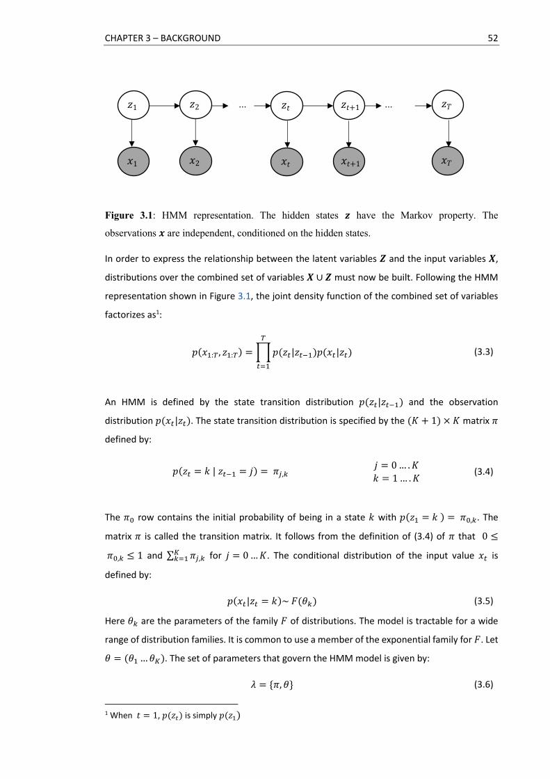
CHAPTER 3 – BACKGROUND 52
Figure 3.1: HMM representation. The hidden states 𝒛 have the Markov property. The
observations 𝒙 are independent, conditioned on the hidden states.
In order to express the relationship between the latent variables 𝒁 and the input variables 𝑿,
distributions over the combined set of variables 𝑿 ∪ 𝒁 must now be built. Following the HMM
representation shown in Figure 3.1, the joint density function of the combined set of variables
factorizes as1:
𝑝(𝑥1:𝑇, 𝑧1:𝑇) = ∏ 𝑝(𝑧𝑡|𝑧𝑡−1)𝑝(𝑥𝑡|𝑧𝑡)
𝑇
𝑡=1
(3.3)
An HMM is defined by the state transition distribution 𝑝(𝑧𝑡|𝑧𝑡−1) and the observation
distribution 𝑝(𝑥𝑡|𝑧𝑡). The state transition distribution is specified by the (𝐾 + 1) × 𝐾 matrix 𝜋
defined by:
𝑝(𝑧𝑡 = 𝑘 | 𝑧𝑡−1 = 𝑗) = 𝜋𝑗,𝑘 𝑗 = 0 … . 𝐾
(3.4) 𝑘 = 1 … . 𝐾
The 𝜋0 row contains the initial probability of being in a state 𝑘 with 𝑝(𝑧1 = 𝑘 ) = 𝜋0,𝑘. The
matrix 𝜋 is called the transition matrix. It follows from the definition of (3.4) of 𝜋 that 0 ≤
𝜋0,𝑘 ≤ 1 and ∑ 𝜋𝑗,𝑘𝐾𝑘=1 for 𝑗 = 0 … 𝐾. The conditional distribution of the input value 𝑥𝑡 is
defined by:
Here 휃𝑘 are the parameters of the family 𝐹 of distributions. The model is tractable for a wide
range of distribution families. It is common to use a member of the exponential family for 𝐹. Let
휃 = (휃1 … 휃𝐾). The set of parameters that govern the HMM model is given by:
𝜆 = {𝜋, 휃} (3.6)
1 When 𝑡 = 1, 𝑝(𝑧𝑡) is simply 𝑝(𝑧1)
𝑝(𝑥𝑡|𝑧𝑡 = 𝑘)~ 𝐹(휃𝑘) (3.5)
... 𝑧1 𝑧2 𝑧𝑡 𝑧𝑡+1
... 𝑧𝑇
𝑥1 𝑥2 𝑥𝑡 𝑥𝑡+1
𝑥𝑇

CHAPTER 3 – BACKGROUND 53
3.1.1 Inference
The marginal distributions 𝑝(𝑧𝑡|𝑥1:𝑡) and 𝑝(𝑧𝑡|𝑥1:𝑇), 𝑇 > 𝑡 are of particular interest when
performing inference in an HMM. The former, referred as filtering, is used to estimate the state
𝑧𝑡 given all observations at times up to and including 𝑡. The latter, referred as smoothing, is used
to estimate the present state conditioned on the past and future observations.
The message passing technique outlined in Appendix D.3 can be used to compute the marginal
distribution 𝑧𝑡 in both cases. Note that in the case of an HMM, there are additional observation
nodes that are conditioned upon during inference. The messages in equations (D.17) and (D.18)
are updated to include the conditional distribution of the observations and are now written as:
𝑚𝑡−1,𝑡(𝑧𝑡) = ∑ 𝑝(𝑥𝑡−1|𝑧𝑡−1)𝑝(𝑧𝑡|𝑧𝑡−1)𝑚𝑡−2,𝑡−1(𝑧𝑡−1)
𝑧𝑡−1
(3.7)
𝑚𝑡+1,𝑡(𝑧𝑡) = ∑ 𝑝(𝑥𝑡+1|𝑧𝑡+1)𝑝(𝑧𝑡+1|𝑧𝑡)𝑚𝑡+2,𝑡+1(𝑧𝑡+1)
𝑧𝑡+1
(3.8)
The marginals can then be computed from the messages as follows:
𝑝(𝑧𝑡|𝑥1:𝑡) ∝ 𝑝(𝑥𝑡|𝑧𝑡)𝑚𝑡−1,𝑡(𝑧𝑡) (3.9)
𝑝(𝑧𝑡|𝑥1:𝑇) ∝ 𝑝(𝑥𝑡|𝑧𝑡)𝑚𝑡−1,𝑡(𝑧𝑡)𝑚𝑡+1,𝑡(𝑧𝑡) (3.10)
The above message based representation of the marginals can also be derived using the
forward-backward algorithm [32]. This classical algorithm defines two terms 𝛼𝑡(𝑧𝑡) and 𝛽𝑡(𝑧𝑡).
The former term is a forward message that represents the joint probability of a state 𝑧𝑡 and the
observations up to time 𝑡. The latter term is a backward message that represents the conditional
probability of all future observations from time 𝑡 + 1 to 𝑇 given the state as 𝑧𝑡. These terms
relate to the messages in (3.7) and (3.8) as follows:
𝛼𝑡(𝑧𝑡) = 𝑝(𝑥1, … , 𝑥𝑡 , 𝑧𝑡) = 𝑝(𝑥𝑡|𝑧𝑡)𝑚𝑡−1,𝑡(𝑧𝑡) (3.11)
𝛽𝑡(𝑧𝑡) = 𝑝(𝑥𝑡+1, … , 𝑥𝑇|𝑧𝑡) = 𝑚𝑡+1,𝑡(𝑧𝑡) (3.12)

CHAPTER 3 – BACKGROUND 54
Figure 3.2: Viterbi decoding. Each circle represents one of the possible states at a time instant
and the lines denote a possible path for the state sequence. The Viterbi algorithm determines the
most probable sequence of states (1, 2, 2, 3 here).
In some inference situations, it is useful to find the most probable sequence of hidden states for
a given observation sequence (see Figure 3.2). Maximizing the marginals 𝑝(𝑧𝑡|𝑥1:𝑇) individually
at each node may not yield the most likely state sequence and may even produce an infeasible
sequence. In detail, we wish to find:
�̂� = argmax𝑧1..𝑧𝑇
∏ 𝑝(𝑧𝑡|𝑧𝑡−1)𝑝(𝑥𝑡|𝑧𝑡)
𝑇
𝑡=1
(3.13)
The same technique used to distribute the summations efficiently for computing the marginals
can be applied here, with the summations now replaced by maximization. Let us define a new
term 𝛿𝑡(𝑧𝑡) such that
𝛿𝑡(𝑧𝑡) = max𝑧1..𝑧𝑡
𝑝(𝑥𝑡|𝑧𝑡)𝑚𝑡−1,𝑡′ (𝑧𝑡) (3.14)
𝑚𝑡−1,𝑡′ (𝑧𝑡) = max
𝑧1..𝑧𝑡−1
𝑝(𝑥𝑡−1|𝑧𝑡−1)𝑝(𝑧𝑡|𝑧𝑡−1)𝑚𝑡−2,𝑡−1′ (𝑧𝑡−1) (3.15)
The maximizing assignment can then be found from the 𝛿 terms. This yields the Viterbi algorithm
that efficiently finds the most likely state sequence with a time complexity that grows linearly
with the number of observations.
3.2 Conditional Random Fields
The Conditional Random Field (CRF) [33] is a probabilistic method that combines the advantages
of discriminative classification techniques with graphical modelling. It is widely used for labelling
sequential data. It is an undirected graphical model belonging to the family of Markov networks.
States
...
...
...
Time
𝑡 = 1 𝑡 = 2 𝑡 = 3 𝑡 = 4
𝑘 = 1
𝑘 = 2
𝑘 = 3

CHAPTER 3 – BACKGROUND 55
CRFs have been applied successfully in computational biology [52], computer vision [53] and
natural language processing [54].
In a CRF, there is a discrete random variable 𝑌𝑡 at each time instant 𝑡. Let 𝑦𝑡 be the value assigned
to 𝑌𝑡. Given an input sequence 𝒙, the output sequence 𝒚 = {𝑦𝑡}𝑡=1𝑇 is predicted. The outputs
are usually class labels. In a classic example, 𝒙 is a sequence of words and 𝒚 is the sequence of
part-of-speech labels for each word. There is a finite number 𝐾 of the labels and 𝑦𝑡 ∈
{1, 2, … 𝐾}. The Markov assumption is applied to the outputs in order to simplify the graph
structure. The resulting model is referred as a Linear Chain CRF.
In a linear chain CRF, the relationship between the combined set of input and output variables
𝑿 ∪ 𝒀 is given by a conditional distribution. Let 𝜓 denote a potential function with values in ℝ.
The conditional distribution 𝑝(𝒚|𝒙) factorizes in linear chain CRF as follows:
𝑝(𝒚|𝒙) =1
𝒵(𝒙) ∏ 𝜓𝑡(𝑦𝑡 , 𝑦𝑡−1, 𝑡, 𝒙)
𝑇
𝑡=1
(3.16)
Here 𝒵(𝒙) is normalization factor over all output sequences given an input sequence 𝒙.
𝒵(𝒙) = ∑ ∏ 𝜓𝑡(𝑦𝑡 , 𝑦𝑡−1, 𝑡, 𝒙)
𝑇
𝑡=1𝒚
(3.17)
The conditional dependency of each output on the inputs is defined in CRFs through a set of real
valued functions called the feature functions. A feature function 𝜑 is defined as follows:
𝜑: 𝒚, 𝒙, 𝑡 → ℝ (3.18)
It can be understood as a feature on the input sequence that determines the likelihood of an
output value at a time instant. It is not required to have a probabilistic interpretation for the
range of a feature function. It is common to have a number of feature functions at each time
instant and they may be nonzero only for a particular output. Consider for example that the
input is a sequence of words and the outputs are the category of each word such as Name,
Location etc. A feature function may be defined to have a value 1 if and only if the output at 𝑦𝑡
is a Location and the input at 𝑥𝑡 appear in a list of country names. The exact form of the feature
functions is problem specific.

CHAPTER 3 – BACKGROUND 56
Figure 3.3: Linear Chain CRF. The outputs follow a Markov assumption. The dashed line edge
between nodes 𝑦𝑡+1 and 𝑥𝑡 illustrates an output 𝑦𝑡+1 depending on the input observations 𝑥𝑡 and
𝑥𝑡+1.
The CRF model is parameterized by a set of real-valued weights, one for each feature function.
Let 휃𝑙 be the weight corresponding to a feature function 𝜑𝑙. The potential function 𝜓𝑡 at time
instant 𝑡 is defined as follows in a linear chain CRF:
𝜓𝑡(𝑦𝑡, 𝑦𝑡−1, 𝑡, 𝒙) = exp {∑ 휃𝑙𝜑𝑙(𝑦𝑡 , 𝑦𝑡−1, 𝑡, 𝒙)
𝐿
𝑙=1
} (3.19)
The main advantage of the CRF is that it does not make any conditional independence
assumptions among the input observations and it can model interdependent features. Hence it
is better suited to cases in which the features overlap. This is evident in (3.19), where the feature
function accepts the entire set of input variables 𝒙 and has the flexibility to examine all these
input variables. Figure 3.3 depicts the graphical model of a linear chain CRF.
The message passing technique derived for the HMM can be used unchanged for the linear chain
CRF. The only difference is in the interpretation. Instead of the conditional distributions used in
the HMM, the potential function as defined in (3.19) is used in the linear chain CRF. The
messages in (3.7) and (3.8) are now written as:
𝑚𝑡−1,𝑡(𝑦𝑡) = ∑ 𝜓𝑡(𝑦𝑡, 𝑦𝑡−1, 𝑡, 𝒙)𝑚𝑡−2,𝑡−1(𝑦𝑡−1)
𝑦𝑡−1
, (3.20)
𝑚𝑡+1,𝑡(𝑦𝑡) = ∑ 𝜓𝑡(𝑦𝑡+1, 𝑦𝑡 , 𝑡, 𝒙)𝑚𝑡+2,𝑡+1(𝑦𝑡+1)
𝑦𝑡+1
. (3.21)
3.3 Nonparametric Models
The statistical models discussed above use a fixed number of parameters and the parameter
space has a finite dimension. In contrast to these parametric models, a nonparametric model
uses an unbounded number of parameters and the parameter space is infinite dimensional.
... 𝑦1 𝑦2 𝑦𝑡 𝑦𝑡+1
... 𝑦𝑇
𝑥1 𝑥2 𝑥𝑡 𝑥𝑡+1
𝑥𝑇

CHAPTER 3 – BACKGROUND 57
Even though there are an unbounded number of parameters, only a finite subset of these
parameters are used to explain a given dataset. The number of parameters may grow (or shrink)
depending on the data.
Several well-known problems benefit from using a nonparametric method. Consider the
traditional finite mixture modelling approach to clustering in which the number of clusters (i.e.
mixtures) are specified in advance. In a nonparametric model, the number of clusters needed to
model the data is estimated from the observed data and new clusters are instantiated as new
data points are observed. If the complexity of the model is measured by the number of clusters
used, it is evident that in a nonparametric model the effective complexity adapts to the data.
The nonparametric models have been applied to a wide range of machine learning problems
including clustering, classification, regression and sequence learning [18].
3.3.1 Dirichlet Process
In a Bayesian approach the parameters are treated as random variables and are assigned prior
distributions. Bayesian nonparametric methods define a prior over an infinite dimensional
parameter space in such a way that the number of parameters used vary with the data
complexity. The Dirichlet Process (DP) [42, 19] is a commonly used nonparametric prior over the
infinite dimensional space of distributions. It is a distribution over probability distributions. Each
sample drawn from a DP is a discrete distribution. Tractable posterior inference procedures can
be developed when employing a DP prior, making it practically useful.
There are several perspectives on the Dirichlet Process. The DP can be constructed from finite-
dimensional Dirichlet distributions. It can also be defined implicitly by an underlying process that
generates a sequence of random variables. Yet another perspective is to describe the random
draw from a Dirichlet Process explicitly using a so-called stick-breaking construction. Finally, the
DP can be viewed as the infinite limit of finite mixture models. These perspectives are mentioned
below.
Let 𝐻 be a distribution over a probability space Θ and 𝛾 be a positive real number. Let (𝐴1, … 𝐴𝐾)
be a partition over Θ such that ⋃ 𝐴𝑘𝐾𝑘=1 = Θ and 𝐴𝑘 ∩ 𝐴𝑗 = ∅, ∀ 𝑘 ≠ 𝑗. A random probability
distribution 𝐺0 is Dirichlet Process distributed if for every partition of Θ, the joint distribution of
random probabilities is Dirichlet distributed as follows:
(𝐺0(𝐴1), … , 𝐺0(𝐴𝐾))~ 𝐷𝑖𝑟(𝛾𝐻(𝐴1), … , 𝛾𝐻(𝐴𝐾)) (3.22)
The draw from a Dirichlet process is denoted as 𝐺0~𝐷𝑃(𝛾, 𝐻), where the base distribution 𝐻 is
the mean of the DP and the concentration parameter 𝛾 can be interpreted as an inverse

CHAPTER 3 – BACKGROUND 58
variance that controls the variability around 𝐻. A larger value for 𝛾 will result in the DP
concentrating its mass around the mean.
It is possible to draw samples from 𝐺0 because 𝐺0 is a random distribution. Let 𝜙1, … , 𝜙𝑖, … , 𝜙𝑛
be a sequence of independent samples drawn from 𝐺0 with each 𝜙𝑖 taking values in Θ. The
posterior distribution of the DP is given as follows:
(𝐺0(𝐴1), … , 𝐺0(𝐴𝐾)) |𝜙1, … 𝜙𝑛 ~ 𝐷𝑖𝑟(𝛾𝐻(𝐴1) + 𝑁1, … , 𝛾𝐻(𝐴𝐾) + 𝑁𝐾) (3.23)
Here 𝑁𝑘 = #{𝑖: 𝜙𝑖 ∈ 𝐴𝑘} denotes the number of samples in 𝐴𝑘. The posterior distribution of
the DP is also a DP. Thus the DP provides a conjugate prior over distributions, a desirable
property that simplifies posterior computation.
The values drawn from 𝐺0 are repeated because it is a discrete distribution. Let 휃1, … , 휃𝑘, … 휃𝐾
be the unique values among 𝜙1, … 𝜙𝑛 and 𝑁𝑘 be the number of times 휃𝑘 is observed.
Marginalizing out 𝐺0, a new value 𝜙𝑛+1 is sampled as follows:
𝜙𝑛+1| 𝜙1 … 𝜙𝑛 ~ ∑𝑁𝑘
𝛾 + 𝑛𝛿𝜃𝑘
𝐾
𝑘=1
+ 𝛾
𝛾 + 𝑛𝐻 (3.24)
where 𝛿𝜃 is an atom located at 휃. The probability that 휃𝑘 will be repeated depends on the
number of times it has already been observed.
The unique 휃𝑘 values induce a random partition of the set {1, … , 𝑛} into clusters. Consider the
set of 𝜙𝑖’s with identical 휃𝑘 values as belonging to a cluster 𝑘. The above sampling scheme
assigns an observation into an existing cluster 𝑘 with a probability that depends on the number
𝑁𝑘 of observations already assigned to the cluster and creates a new cluster with probability
𝛾
𝛾+𝑛. The larger 𝑁𝑘 is, the higher the probability that cluster 𝑘 will be assigned more observations.
Larger clusters grow larger, faster. This implies a rich-gets-richer phenomenon that is desirable
in clustering.
The above distribution over the partitions is understood intuitively by the Chinese Restaurant
Process metaphor shown in Figure 3.4. There is a restaurant with an infinite number of tables
(clusters). The first customer is seated at the first table. A second customer sits either at the first
table or in a new table. In general, the (𝑛 + 1)𝑡ℎ customer joins an already occupied table with
probability proportional to the number 𝑁𝑘 of customers already seated at table 𝑘. The customer
can also choose a new table with probability proportional to 𝛾.

CHAPTER 3 – BACKGROUND 59
Figure 3.4: Chinese Restaurant Process. The circles denote the tables and 휃𝑘 is the unique value
associated with table 𝑘. The diamonds represent the customers with 𝜙𝑛 being the 𝑛𝑡ℎ customer.
A new customer selects an existing table with a probability proportional to the number of
customers already seated at a table. A new table may also be selected.
The stick-breaking representation [43] shows explicitly the discreteness of the random
distributions drawn from a DP. The random distribution 𝐺0 can be determined by drawing an
unbounded number of samples from a Beta distribution and the base distribution 𝐻. The
generation process is as follows:
𝛽𝑘′ | 𝛾 ~ 𝐵𝑒𝑡𝑎(1, 𝛾) 𝛽𝑘 = 𝛽𝑘
′ ∏(1 − 𝛽𝑙′)
𝑙<𝑘
𝑘 = 1,2 … (3.25)
휃𝑘 | 𝐻 ~ 𝐻 𝑘 = 1,2 … (3.26)
𝐺0 = ∑ 𝛽𝑘𝛿𝜃𝑘
∞
𝑘=1
(3.27)
The values 휃𝑘 are drawn independently from the base distribution 𝐻 and 𝛽𝑘 is a probability
associated with the atom 𝛿𝜃𝑘 and ∑ 𝛽𝑘
∞𝑘=1 = 1. The construction of 𝛽𝑘 can be understood
metaphorically by the division of a stick into an infinite number of segments as depicted in Figure
3.5. We start with an unit length stick, choose 𝛽1′ according to (3.25) and break the stick at 𝛽1
′ .
For the remaining segment, we choose 𝛽2′ and break off the 𝛽2
′ proportion of the remainder of
the stick and so on. This provides a distribution on the strictly positive integers. It is common to
write the weights 𝛽 = {𝛽𝑘}𝑘=1∞ obtained using (3.25) as 𝛽 ~ 𝐺𝐸𝑀(𝛾), named after Griffiths,
Engen, and McCloskey.
The above representation is useful in the interpretation of the DP as the infinite dimensional
generalization of a finite parametric model. Consider a finite mixture with 𝐾 components. The
density for this mixture model over observations 𝑥 is represented as follows:
휃1
𝜙1
𝜙6
𝜙3
휃2
𝜙2
𝜙7
𝜙8
휃3
𝜙4
𝜙5
𝜙2
휃4

CHAPTER 3 – BACKGROUND 60
Figure 3.5: Dirichlet Process. Left: A representation of the Dirichlet Process mixture in a
graphical format. The variables are represented as nodes in the graph. The latent variable 𝑧𝑛
indicates the mixture component an observation 𝑥𝑛 belongs to. The replicated variables are
compactly represented using the plate notation [29]. The rectangles denote replication with the
number of replicates given in the bottom right corner. Right: The stick breaking construction. The
stick is broken at 𝛽𝑘′ and subsequent weights 𝛽𝑘+1 are obtained as random proportions of this
segment.
𝑝(𝑥) = ∑ 𝑤𝑘 𝑝(𝑥|휃𝑘)
𝐾
𝑘=1
(3.28)
Here 𝑤𝑘 is the weight for the 𝑘𝑡ℎ component of the mixture and 휃𝑘 is a set of parameters
associated with the 𝑘𝑡ℎ component. This density can also be written as
𝑝(𝑥) = ∫ 𝑝(𝑥|휃)𝐺0(휃)𝑑휃 (3.29)
where 𝐺0 is a mixing discrete distribution and is defined as follows:
𝐺0 = ∑ 𝑤𝑘𝛿𝜃𝑘
𝐾
𝑘=1
(3.30)
In the nonparametric extension to the finite mixtures, the mixing distribution in equation (3.27)
is used instead of (3.30). This gives rise to a mixture model with an unbounded number of
mixture components. The DP is used as a prior over 𝐺0 and the resulting mixture model is called
the DP mixture [42]. The 𝛽𝑘 terms in (3.27), which defines a probability distribution on the set
ℤ+, is interpreted as the mixture weights. This probability distribution is chosen at random via
the stick breaking process.
𝑧𝑛
𝑁
∞
𝐻
𝛽 𝛾
𝑥𝑛
휃𝑘
𝛽1 𝛽2
𝛽1′ 1 − 𝛽1
′

CHAPTER 3 – BACKGROUND 61
The process by which observations are generated from a Dirichlet process mixture with
concentration parameter 𝛾 and base distribution 𝐻 is described as follows:
(i) Generate the stick breaking weights 𝛽 as 𝛽 | 𝛾 ~ 𝐺𝐸𝑀(𝛾)
(ii) Draw independent samples of the parameters from the base distribution as
휃𝑘 | 𝐻 ~ 𝐻, 𝑘 = 1, 2 ….
(iii) Draw a latent variable 𝑧𝑛 that indicates the mixture component that the 𝑛𝑡ℎ
observation belongs to. This is done using the stick breaking weights and is denoted
as 𝑧𝑛 | 𝛽 ~ 𝛽, 𝑛 = 1 … 𝑁.
(iv) Draw an observation 𝑥𝑛 given the latent variables and the parameters as
𝑥𝑛 | 𝑧𝑛, {휃𝑘}𝑘=1∞ ~ 𝐹(휃𝑧𝑛
), 𝑘 = 1,2, … 𝑛 = 1, … 𝑁. Here 𝐹 denotes the
distribution family of the mixture component using 휃 as its parameter.
Figure 3.5 illustrates this process. In the Dirichlet process mixture, the mixture component 𝑘 is
described by the distribution 𝐹(휃𝑘). Note that the 𝜙𝑛 discussed in the Chinese restaurant
process is simply 휃𝑧𝑛. The probability that an observation is assigned to the 𝑘𝑡ℎ component is
𝛽𝑘 . Note that the number of components 𝐾 → ∞. Thus the DP can be used to model a mixture
with no upper bound on the number of components.
3.3.2 Hierarchical Dirichlet Process
In many situations, we encounter data organized into distinct groups. There is a need to capture
both the similarities and differences across the individuals within these groups. As an example,
consider the problem of modelling the topics [183] embedded in a corpus of documents. A
document consists of a number of words which arise from a set of underlying semantic themes
referred as topics. We want to describe the way in which the topics are shared across the
documents and yet capture the document specific properties of a topic – i.e. we wish to share a
common set of clusters (topics) among several related groups (documents). The Dirichlet
Process as such cannot be used to model grouped data. The need to share clusters among groups
motivates the use of a hierarchical model.
The Hierarchical Dirichlet Process (HDP) [44] is an extension of the DP. It is used to model groups
of data. Each group has a separate DP prior but all these DPs are linked through a global DP. This
provides a mechanism for inferring group specific probability masses while at the same time
sharing parameters across the groups.
As before, let 𝐺0 denote a draw from a Dirichlet Process with concentration parameter 𝛾 and a
base distribution 𝐻. The HDP defines a set of random distributions {𝐺𝑗}𝑗=1𝐽 over 𝐽 groups of

CHAPTER 3 – BACKGROUND 62
data. Given the global distribution 𝐺0, the set of distributions over the 𝐽 groups are conditionally
independent.
𝐺0 | 𝛾, 𝐻 ~ 𝐷𝑃(𝛾, 𝐻) (3.31)
𝐺𝑗| 𝛼, 𝐺0 ~ 𝐷𝑃(𝛼, 𝐺0) 𝑗 = 1, … 𝐽 (3.32)
The 𝑗𝑡ℎ group’s distribution 𝐺𝑗 contains values drawn from 𝐺0 with 𝛼 ∈ ℝ+ controlling the
variability around 𝐺0. The distribution 𝐺0 can be interpreted as the mean distribution across all
the groups.
Figure 3.6: Chinese Restaurant Franchise. The diamonds represent the customers with 𝜙𝑗𝑛 being
the 𝑛𝑡ℎ customer at restaurant 𝑗. The circles denote the tables. The dishes are shared across the
restaurants with the dish (parameter) 휃3 being re-used. The tables and dishes are selected based
on the proportion of them being used. A new table or a new dish may also be selected.
The HDP can also be described using a metaphor, now called the Chinese Restaurant Franchise
illustrated in Figure 3.6. There are now 𝐽 restaurants (each corresponding to an HDP group) with
all the restaurants sharing a single menu of an infinite number of dishes (parameters). Let 𝜙𝑗𝑛
denote the 𝑛𝑡ℎ customer from the 𝑗𝑡ℎ restaurant. Let 휃1, … , 휃𝑘, … 휃𝐾 be the dishes served
휃̅11 = 휃1
𝜙13
𝑗 = 1
𝜙11
𝜙16
𝜙12
𝜙14
𝜙15
𝜙21
𝑗 = 2
𝜙24
𝜙23
𝜙25
𝜙22
𝜙26
휃3
휃2
휃1
휃̅12 = 휃3 휃̅13 = 휃3
휃̅21 = 휃2 휃̅22 = 휃2 휃̅23 = 휃3
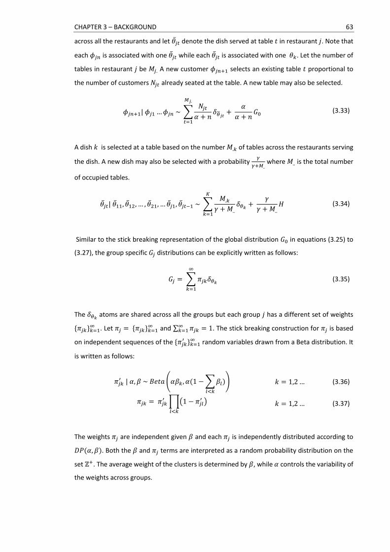
CHAPTER 3 – BACKGROUND 63
across all the restaurants and let 휃̅𝑗𝑡 denote the dish served at table 𝑡 in restaurant 𝑗. Note that
each 𝜙𝑗𝑛 is associated with one 휃̅𝑗𝑡 while each 휃̅𝑗𝑡 is associated with one 휃𝑘. Let the number of
tables in restaurant 𝑗 be 𝑀𝑗. A new customer 𝜙𝑗𝑛+1 selects an existing table 𝑡 proportional to
the number of customers 𝑁𝑗𝑡 already seated at the table. A new table may also be selected.
𝜙𝑗𝑛+1| 𝜙𝑗1 … 𝜙𝑗𝑛 ~ ∑𝑁𝑗𝑡
𝛼 + 𝑛𝛿�̅�𝑗𝑡
𝑀𝑗.
𝑡=1
+ 𝛼
𝛼 + 𝑛𝐺0 (3.33)
A dish 𝑘 is selected at a table based on the number 𝑀.𝑘 of tables across the restaurants serving
the dish. A new dish may also be selected with a probability 𝛾
𝛾+𝑀.. where 𝑀.. is the total number
of occupied tables.
휃̅𝑗𝑡| 휃̅11, 휃̅12, … , 휃̅21, … 휃̅𝑗1, 휃̅𝑗𝑡−1 ~ ∑𝑀.𝑘
𝛾 + 𝑀..𝛿𝜃𝑘
𝐾
𝑘=1
+ 𝛾
𝛾 + 𝑀..𝐻 (3.34)
Similar to the stick breaking representation of the global distribution 𝐺0 in equations (3.25) to
(3.27), the group specific 𝐺𝑗 distributions can be explicitly written as follows:
𝐺𝑗 = ∑ 𝜋𝑗𝑘𝛿𝜃𝑘
∞
𝑘=1
(3.35)
The 𝛿𝜃𝑘 atoms are shared across all the groups but each group 𝑗 has a different set of weights
{𝜋𝑗𝑘}𝑘=1∞ . Let 𝜋𝑗 = {𝜋𝑗𝑘}𝑘=1
∞ and ∑ 𝜋𝑗𝑘∞𝑘=1 = 1. The stick breaking construction for 𝜋𝑗 is based
on independent sequences of the {𝜋𝑗𝑘′ }𝑘=1
∞ random variables drawn from a Beta distribution. It
is written as follows:
𝜋𝑗𝑘′ | 𝛼, 𝛽 ~ 𝐵𝑒𝑡𝑎 (𝛼𝛽𝑘 , 𝛼(1 − ∑ 𝛽𝑙
𝑙<𝑘
)) 𝑘 = 1,2 … (3.36)
𝜋𝑗𝑘 = 𝜋𝑗𝑘′ ∏(1 − 𝜋𝑗𝑙
′ )
𝑙<𝑘
𝑘 = 1,2 … (3.37)
The weights 𝜋𝑗 are independent given 𝛽 and each 𝜋𝑗 is independently distributed according to
𝐷𝑃(𝛼, 𝛽). Both the 𝛽 and 𝜋𝑗 terms are interpreted as a random probability distribution on the
set ℤ+. The average weight of the clusters is determined by 𝛽, while 𝛼 controls the variability of
the weights across groups.

CHAPTER 3 – BACKGROUND 64
Figure 3.7: Hierarchical Dirichlet Process. A representation of the HDP used as a nonparametric
prior for clustering grouped data. The variables are represented as nodes in the graph. The
concentration parameters 𝛾, 𝛼 and the prior 𝐻 are shown as text. The latent variable 𝑧𝑗𝑛 indicates
the mixture component an observation 𝑥𝑗𝑛 belongs to. The parameter 휃𝑘 is shared by all groups
while the mixture proportion 𝜋𝑗 may vary among the groups. The plate notation is used.
While the DP is used as a prior for a mixture model for clustering data, the HDP is used as a
nonparametric prior distribution for a set of mixture models that are used for clustering grouped
data. The process by which observations are generated based on the HDP is given as follows:
𝛽 | 𝛾 ~ 𝐺𝐸𝑀(𝛾)
(3.38)
𝜋𝑗 | 𝛼, 𝛽 ~ 𝐷𝑃(𝛼, 𝛽) 𝑗 = 1, … 𝐽
휃𝑘 | 𝐻 ~ 𝐻 𝑘 = 1,2, …
𝑧𝑗𝑛 | 𝜋𝑗 ~ 𝜋𝑗 𝑗 = 1, … 𝐽, 𝑛 = 1 … 𝑁
𝑥𝑗𝑛 | 𝑧𝑗𝑛, {휃𝑘}𝑘=1∞ ~ 𝐹(휃𝑧𝑗𝑛
) 𝑗 = 1, … 𝐽, 𝑛 = 1 … 𝑁
Here 𝑧𝑗𝑛 is a latent variable that indicates the mixture component that the 𝑗𝑡ℎ group’s 𝑛𝑡ℎ
observation 𝑥𝑗𝑛 belongs to. The 𝜙𝑗𝑛 discussed in the Chinese restaurant Franchise is 휃𝑧𝑗𝑛. For a
given component 𝑘, all the 𝐽 groups share the same set of parameters 휃𝑘 but the 𝑗𝑡ℎ group uses
𝜋𝑗𝑘 proportion. This process is shown in Figure 3.7.
This thesis uses HDP extensively to enable construction of nonparametric models.
𝜋𝑗
𝐽
∞
𝐻
𝛽 𝛾
휃𝑘
𝛼
𝑧𝑗𝑛
𝑥𝑗𝑛
𝑁

65
4. Discriminative nonparametric HMM
In this chapter, a nonparametric HMM based on the Hierarchical Dirichlet Process (HDP) is
proposed for classifying human actions. The proposed model addresses an important limitation
of the classical HMM, namely the need to fix the number of hidden states a-priori. The novel
construction provided here produces a flexible model that is better suited for classification tasks.
The formulation enables information sharing and allows the use of unlabelled examples.
The chapter begins with an overview of the proposed approach in Section 4.1 and introduces
the HDP-HMM in Section 4.2. Instead of using separate models for each action class, a single
HDP-HMM is used to model all the actions. In order to distinguish between the actions, the HDP
is extended by an additional level and class specific transformations are introduced for the
distributions of HDP parameters. Section 4.3 elaborates on this model structure. During training,
the parameters are learnt in a discriminative manner. This process is discussed in Section 4.4
and is followed in Section 4.5 by the derivation of the posterior inference procedure.
Experiments are conducted on two different publicly available datasets that contain depth
image sequences. The information in the skeletal joint positions is used to classify the actions
using the proposed model. The results are presented in Section 4.6. The chapter ends with some
concluding remarks in Section 4.7. Portions of this chapter have been published [192, 193].
4.1 Overview
Depth sensors such as Kinect, with inbuilt human motion capturing techniques, provide
estimates of a human skeleton’s 3D joint positions over time [14]. High level actions can be
inferred from these joint positions. However, robust and accurate inference is still a problem.
Given a sequence of 3D joint positions, a state space model such as a Hidden Markov Model
(HMM) is a natural way to represent an action class. The HMMs are proven models for
sequential pattern recognition [48, 49, 50]. Recall that in an HMM, a sequence of discrete state
variables are linked in a Markov chain by a state transition matrix. Each observation is drawn
independently from a distribution conditioned on the appropriate state [32]. If each action class
is represented using an HMM, the model parameters corresponding to a given class, namely the
state transition matrix and the state specific observation distributions, can be learnt from

CHAPTER 4 – NONPARAMETRIC HMM 66
examples belonging to that class. The prediction of a new input’s class is obtained from the class
conditional posterior densities.
In classical parametric HMMs, the number of states must be specified a-priori. In many
applications this number is not known in advance. For instance, there is no a-priori knowledge
about the number of intermediate poses that comprises an action. This number will vary
depending on the complexity of the action and the number of subjects in the data set. A typical
solution to this problem is to carry out training using different choices for the number of states
and then apply a model selection criterion to find the best result. There is little understanding
of the strengths and weaknesses of this procedure and often complex application specific tuning
is involved.
Instead of this ad hoc model selection, it is preferable to estimate the correct number of states
automatically from data. This allows the model complexity to adapt to the size of the data set.
The nonparametric methods [18, 19] provide the necessary statistical framework to model the
data with an unbounded number of parameters. The number of parameters grows with the
sample size. In [44], a nonparametric Bayesian method, the Hierarchical Dirichlet Process (HDP),
is defined. The HDP is used to construct an HMM with an unbounded set of states. The prior
distribution on the HMM transition matrix is over an infinite state space but for a given set of
observations, only a finite number of the states is used to explain the data.
It would be straight forward to use separate HDP-HMMs for each action class and train them
individually. However, this would prohibit the sharing of training examples across the action
classes. To see the merit of sharing examples, consider that an action is a sequence of poses. It
is quite likely that two or more actions share many similar poses with possibly a few poses
unique to particular actions. In fact, two actions such as ‘stand-up’ and ‘sit-down’, may have the
same set of poses with only the temporal order of pose sequences differing. What necessarily
differentiates one action from another are the transition probabilities of the poses. If a particular
pose is absent from an action class then there is a low probability of transition to the state for
that pose. In this work, a single HDP-HMM is used to model all the action classes. The canonical
HDP-HMM is extended with an additional class specific hierarchical level that accounts for
differences in the state transition probabilities among the action classes.
In the canonical construction of the HDP-HMM, the mixture components are shared across the
hierarchical levels. It would be more flexible to allow the mixture components of an action class
to vary slightly from the other classes; i.e. we seek a class specific transformation of the shared
mixture component parameters so that the classes can be discriminated in a better manner.
Note that this is different from using individually trained HDP-HMM models where the

CHAPTER 4 – NONPARAMETRIC HMM 67
component parameters are not shared among the classes. In this work, the mixture components
are assumed to have Gaussian distributions, and class specific affine transformations of the
Gaussian distribution parameters (mean and covariance) are used. An overview of the approach
is provided in Figure 4.1.
Figure 4.1: Discriminative HDP-HMM overview. Training examples contain joint position
sequences from different action classes. The examples from all these action classes are combined
in order to infer the shared pose transitions and pose definitions. P1, P2, P3 and P4 in the Shared
Parameters group represent the various poses (states). Each pose is defined by a distribution. The
action class specific transitions and distributions are inferred as transformations of this shared
representation. Pose P3 may be absent in the first action class and hence there is a low probability
of transition to it (shown with an absence of arrow to this state). The action class labels in the
training examples and the learned shared parameters are used to infer the class specific
parameters.
The HDP-HMM based classification approach described above defines a joint distribution of the
input data and class labels to train the classifier. This generative model allows the augmentation
of the labelled training examples with unlabelled examples and thus provides a framework for
semi-supervised learning. In contrast, a discriminative model uses the conditional distribution
of the class labels given the input data to train the classifier. This approach often produces good
P 1 P 2
P 4 P 3
P 1 P 2
P 4
P 3
P 1 P 2
P 4
P 3
P 1 P 2
P 4
P 3
Training Examples
Shared Parameters
Class Specific Parameters

CHAPTER 4 – NONPARAMETRIC HMM 68
classification results [64]. For example, Support Vector Machines (SVMs) [65] use a margin based
likelihood that maximizes the distances of the feature vectors to the classification boundary
while minimizing the empirical error rate on the training set. Inspired by this, a margin based
term is incorporated in the likelihood function used in HDP-HMM training. The inclusion of this
discriminative term in the otherwise generative model, compensates for potential model
misspecification and leads to better classification results.
Incorporation of a discriminative term into the HDP-HMM model makes the posterior sampling
less straight-forward. The HDP model as such has no provision for including an additional term
for the mixing proportions. To address this, a normalized gamma process formulation [66] of
the HDP is used. This allows a scaling of the mixing proportions of a DP through a discriminative
weighting term. For the mixture components with Gaussian distribution parameters, the prior
is no longer of the same form as the likelihood and hence is not conjugate. Slice sampling [39]
based techniques allow sampling from any likelihood function, even if the normalization is
unknown. A Gaussian prior is placed on the parameters and Elliptical Slice Sampling [67] is used
to sample the posterior efficiently.
Contributions
The main contributions in this chapter are the construction of a discriminative nonparametric
HMM and the derivation of a tractable inference mechanism. The proposed model has the
following advantages:
(a) The nonparametric formulation allows the number of states to be inferred
automatically.
(b) The use of a single HDP-HMM promotes information sharing.
(c) The discriminative terms ensure that the HDP-HMM is suitable for classification tasks.
(d) The model can be used for semi-supervised learning.
(e) The model is generic, in that it is applicable to other sequence classification problems.
4.2 HDP-HMM
Recall the HMM in Section 3.1. The HMM is parameterized by the transition matrix 𝜋 where the
𝑗𝑡ℎ row of the matrix defines the probabilities of the transitions from the state 𝑗. The hidden
states 𝑧1:𝑇 have the Markov property. The probability of transitioning to a state 𝑧𝑡 at a time
instant 𝑡 from a previous state 𝑧𝑡−1 is specified by the transition matrix. Additionally, there are
state specific observation density parameters {휃𝑘}1𝐾 where 𝐾 is the number of hidden states.
For the Bayesian version of the classical HMM, it is necessary to introduce priors. Note that the
rows of 𝜋 cannot have independent priors because the transitions out of the different states

CHAPTER 4 – NONPARAMETRIC HMM 69
must be coupled. Let the priors be 𝛽 ~ 𝐷𝑖𝑟(𝛾
𝐾) and 𝜋𝑗 ~ 𝐷𝑖𝑟(𝛼𝛽1 … 𝛼𝛽𝐾) where 𝐷𝑖𝑟 is the
Dirichlet distribution and 𝛾, 𝛼 are some positive real numbers. The observation density
parameters are assigned a prior 𝐻. With this definition, an observation is generated in the
Bayesian HMM as follows:
𝛽 | 𝛾 ~ 𝐷𝑖𝑟 (𝛾
𝐾) (4.1)
𝜋𝑗 | 𝛼, 𝛽 ~ 𝐷𝑖𝑟(𝛼𝛽1 … 𝛼𝛽𝐾) 𝑗 = 1, … 𝐾 (4.2)
휃𝑘 | 𝐻 ~ 𝐻 𝑘 = 1, … 𝐾 (4.3)
𝑧𝑡 | 𝜋, 𝑧𝑡−1 ~ 𝜋𝑧𝑡−1 𝑡 = 1, … . 𝑇 (4.4)
𝑥𝑡 | 𝑧𝑡 , {휃𝑘}𝑘=1∞ ~ 𝐹(휃𝑧𝑡
) 𝑡 = 1, … 𝑇 (4.5)
Figure 4.2: Graphical representation of HDP-HMM. The states 𝑧1:𝑇 have the Markov property.
An observation 𝑥𝑡 is conditioned on the state 𝑧𝑡. The states are generated from the transition
matrix 𝜋𝑗 and the observations are generated from the mixture component parameters. The
number of states and the number of mixture components are unbounded.
This generation process is remarkably similar to the process by which the observations are
generated using HDP shown in Equation (3.38), Section 3.3. A group specific 𝜋𝑗 distribution in
the HDP is a state specific distribution in the HMM with the groups in the HDP formulation
corresponding to the states in the HMM. If an HDP prior is assigned over the state transition
matrix, the matrix will have an infinite number of rows and columns with the HDP semantics
ensuring that only a finite subset of these states are actually instantiated. Thus the HMM is now
nonparametric. The HDP-HMM can also be interpreted as an infinite extension of a dynamic
𝑧1 𝑧2 𝑧𝑇
𝑥1 𝑥2 𝑥𝑇
...
𝜋𝑗
∞
𝛼
𝛽 𝛾
𝜇𝑘
, Σ𝑘
∞
𝐻

CHAPTER 4 – NONPARAMETRIC HMM 70
mixture model. The mixture weight of an observation depends on the previous observations and
there are an unbounded number of mixtures.
To complete the definition of the HDP-HMM, let 𝐹 be the Gaussian density. The density
parameters for the observation density associated with state 𝑘 are now the mean 𝜇𝑘 and
covariance Σ𝑘. It is convenient to write 휃𝑘 = (𝜇𝑘 , Σ𝑘). Let the mixture mean have a normal prior
𝜇 ~ 𝒩(𝜇0, Σ0) and let the covariance have an Inverse-Wishart prior Σ ~ 𝐼𝑊(𝜈0, Δ0). An
observation is generated in the nonparametric HMM as follows.
𝛽 | 𝛾 ~ 𝐺𝐸𝑀(𝛾) (4.6)
𝜋𝑗 | 𝛼, 𝛽 ~ 𝐷𝑃(𝛼, 𝛽) 𝑗 = 1,2, … (4.7)
𝜇𝑘 | 𝜇0, Σ0 ~ 𝒩(𝜇0, Σ0) 𝑘 = 1,2, … (4.8)
Σ𝑘 | 𝜈0, Δ0 ~ 𝐼𝑊(𝜈0, Δ0) 𝑘 = 1,2, … (4.9)
𝑧𝑡 | 𝜋, 𝑧𝑡−1 ~ 𝜋𝑧𝑡−1 𝑡 = 1, … . 𝑇 (4.10)
𝑥𝑡 | 𝑧𝑡, {𝜇𝑘 , Σ𝑘}𝑘=1∞ ~ 𝒩(𝜇𝑧𝑡
, Σ𝑧𝑡) 𝑡 = 1, … 𝑇 (4.11)
Figure 4.2 provides a graphical representation of this HDP-HMM.
4.3 Model
Let a training dataset comprising 𝑁 observations 𝑋 = {𝑥𝑛}𝑛=1𝑁 together with labels 𝑌 =
{𝑦𝑛}𝑛=1𝑁 be given. Here 𝑥𝑛 = 𝑥1
𝑛, … , 𝑥𝑡𝑛, … , 𝑥𝑇
𝑛 is an input sequence and 𝑦𝑛 ∈ { 1 … 𝑐 … 𝐶} is
the class label corresponding to the sequence 𝑥𝑛. For example, in action classification, 𝑥𝑛 is an
input image sequence and 𝑦𝑛 is an action class label. The observations and their labels are drawn
independently from the same fixed distribution. Each 𝑥𝑡𝑛 ∈ ℝ𝑑 corresponds to the features
extracted at time step 𝑡 from the input. Further discussion of the features is deferred to Section
4.6. Let the set of all model parameters be 휃. The objective is classification, where given a new
test observation sequence 𝑥, the corresponding action class �̂� must be predicted. A suitable
prediction is
�̂� = argmax𝑐
𝑝(𝑐 | 𝑥, 𝑋, 𝑌) (4.12)
The distribution 𝑝(𝑐 | 𝑥, 𝑋, 𝑌) can be written in the form
𝑝(𝑐 | 𝑥, 𝑋, 𝑌) = ∫ 𝑝(𝑐 | 𝑥, 휃) 𝑝(휃 | 𝑋, 𝑌) 𝑑휃 (4.13)

CHAPTER 4 – NONPARAMETRIC HMM 71
The model proposed in this chapter differs from the canonical HDP-HMM in two key aspects.
First, an extra level in the HDP is introduced to model class specific mixture proportions as
discussed in Section 4.3.1. The second difference is the extension of the HDP parameter space
with class specific distributions for the mean and covariance parameters. This novel formulation
is presented in Section 4.3.2.
4.3.1 Two level HDP
If each action class is represented by a separate HDP-HMM, then 휃𝑐 = {𝛽𝑐 , 𝜋𝑐 , 𝜇1..∞𝑐 , Σ1..∞
𝑐 } are
the parameters for class 𝑐, 휃 = {휃𝑐}𝑐=1𝐶 is the set of all parameters for the different classes and
𝛾, 𝛼, 𝜇0, Σ0, 𝜈0, Δ0 are the hyper parameters. It would be straight forward to estimate the
posterior density of parameters 𝑝(휃 | 𝑋, 𝑌) if each HDP-HMM model were to be trained
separately i.e. a class conditional density 𝑝(𝑥 | 𝑐) can be defined for each class and the posterior
can be estimated from
𝑝(휃𝑐 | 𝑋, 𝑌) = 𝑝(휃𝑐) ∏ 𝑝(𝑥𝑛 | 휃𝑐)𝑝(𝑐)
𝑛:𝑦𝑛=𝑐
(4.14)
However, in this approach the training examples from other classes are not used when learning
the parameters of a class. As noted in Section 4.1, many actions contain similar poses and it is
useful to incorporate pose information from other classes during training. Specifically, the
inclusion of additional observations for a similar pose benefits estimation of the Gaussian
mixture parameters. The state transition parameters must continue to be different for each
action class since it is these parameters that necessarily distinguish the actions.
Instead of separate HDP-HMMs, a single HDP-HMM is defined for all the action classes albeit
with an extra level that is class specific i.e. in addition to the global distribution 𝐺0 and the state
specific distributions 𝐺𝑗 in the canonical HDP, there are now class specific distributions 𝐺𝑗𝑐 for
every state. The two-level HDP-HMM is defined as follows.
𝐺0 | 𝛾, 𝐻 ~ 𝐷𝑃(𝛾, 𝐻) (4.15)
𝐺𝑗 | 𝛼, 𝐺0 ~ 𝐷𝑃(𝛼, 𝐺0) 𝑗 = 1,2, … (4.16)
𝐺𝑗𝑐 | 𝜆, 𝐺𝑗 ~ 𝐷𝑃(𝜆, 𝐺𝑗) 𝑐 = 1, … 𝐶 (4.17)
Just as the 𝐺𝑗s are conditionally independent given 𝐺0, the 𝐺𝑗𝑐s are conditionally independent
given 𝐺𝑗. All the classes for a given state share the same subset of mixture parameters but the
proportions of these mixtures will differ for each class as determined by the positive real valued

CHAPTER 4 – NONPARAMETRIC HMM 72
concentration parameter 𝜆. The varying mixture proportions induce differences in the state
transition probabilities between the action classes and ensure that classification can be
performed.
Recall the stick breaking construction of the canonical HDP presented in Equations (3.35) to
(3.37). The extension of this construction to the additional class specific measure is straight-
forward. In addition to the stick breaking weights 𝛽 and 𝜋, a new weight term 𝜑 is now
introduced to represent the second level. Independent sequences of the {𝜑𝑗𝑘𝑐′
}𝑘=1∞ random
variables are drawn from the Beta distribution (Appendix C.3). The formulation is as follows:
𝜑𝑗𝑘𝑐′
| 𝜆, 𝜋𝑗 ~ 𝐵𝑒𝑡𝑎 (𝜆𝜋𝑗𝑘 , 𝜆(1 − ∑ 𝜋𝑗𝑙
𝑙<𝑘
)) 𝑘 = 1,2 …
(4.18) 𝜑𝑗𝑘𝑐 = 𝜑𝑗𝑘
𝑐′∏ (1 − 𝜑𝑗𝑙
𝑐′)
𝑙<𝑘
𝑘 = 1,2 …
𝐺𝑗𝑐 = ∑ 𝜑𝑗𝑘
𝑐 𝛿𝜃𝑘
∞
𝑘=1
Similar to 𝛽 and 𝜋𝑗, 𝜑𝑗𝑐 = {𝜑𝑗𝑘
𝑐 }𝑘=1∞ can be interpreted as a random probability distribution on
the set ℤ+. Assuming the variables 𝜋𝑗, 𝜇𝑘 and Σ𝑘 are defined as in equations (4.7) to (4.9), the
generative story for an observation 𝑥𝑡𝑛 belonging to class 𝑐, sampled at time 𝑡 from the two level
HDP-HMM is written as
𝜑𝑗𝑐| 𝜆, 𝜋𝑗 ~ 𝐷𝑃(𝜆, 𝜋𝑗)
(4.19) 𝑧𝑡𝑛 | 𝑧𝑡−1
𝑛 , 𝑦𝑛 = 𝑐, {𝜑𝑗𝑐}
𝑗=1,𝑐=1
∞,𝐶 ~ 𝜑𝑧𝑡−1
𝑛𝑐
𝑥𝑡𝑛 | 𝑧𝑡
𝑛, {𝜇𝑘 , Σ𝑘}𝑘=1∞ ~ 𝒩(𝜇𝑧𝑡
𝑛 , Σ𝑧𝑡𝑛)
Consequently, for the two level HDP-HMM, the set of all model parameters is 휃 =
{𝛽, 𝜋, 𝜑1..𝐶 , 𝜇1..∞, Σ1..∞} with 𝛾, 𝛼, 𝜇0, Σ0, 𝜈0, Δ0, 𝜆 as the hyper parameters.
4.3.2 Transformed HDP Parameters
In the HDP, the same mixture component parameters are used by the different groups i.e. the
parameters 휃𝑘 remain the same in all 𝐺𝑗 (and 𝐺𝑗𝑐 in case of an additional level). This is less flexible
than allowing the parameters to vary across the groups. As an example, the position and
orientation of the joints in a squat pose might mostly look the same across action classes such
as sit-up, sit-down and pick-up while it may slightly differ for pick-up class. In this case, it would
be useful to capture the deviation from the standard squat pose for the pick-up action class –

CHAPTER 4 – NONPARAMETRIC HMM 73
i.e. we wish to introduce a transformation of the parameters, one for each action class, from its
canonical form 휃𝑘.
The affine transformation of the Gaussian distribution parameters mean 𝜇 and covariance Σ is
considered here [68]. Let 𝜌 be a vector and let Λ be an invertible matrix. The transformation of
the Gaussian distribution defined by 𝜌, Λ is as follows
𝒩(𝜇, Σ) ⟼ 𝒩(Λ𝜇 + 𝜌, ΛΣΛ𝑇) (4.20)
It is usual to restrict Λ in order to ensure computational tractability. A useful simplification is to
set Λ equal to the identity matrix. This is equivalent to restricting the transformations to a
translation of the Gaussian mean by 𝜌. Other restrictions include requiring Λ to be diagonal, to
account for scaling.
Figure 4.3: Graphical representation of the two level HDP-HMM. The HDP-HMM is extended
with the class specific mixture weights 𝜑𝑗𝑐 and class specific transformation parameters 𝜌𝑘
𝑐 . The
observations on the left side are generated by the parameters for class 𝑐 = 1 while those on the
right side by the parameters for class 𝑐 = 𝐶.
The class specific transformation based on (4.20) is introduced here to the Gaussian mixture
parameters. Let the variable responsible for shifting the mean have a zero mean normal prior
𝜋𝑗
∞
𝛼
𝛽 𝛾
𝑧1 𝑧𝑇
𝑥1 𝑥𝑇
...
𝜑𝑗1
∞
𝜆 𝜑𝑗𝐶 ...
𝐻
∞
𝜌𝑘1 ... 𝜌𝑘
𝐶
𝜇𝑘 , Σ𝑘
𝑧1 𝑧𝑇
𝑥1 𝑥𝑇
...

CHAPTER 4 – NONPARAMETRIC HMM 74
i.e. 𝜌 ~ 𝒩(0, Ω0). The focus here is only on scale transformations. Thus Λ is assumed to be
diagonal. In effect, the scale transform variable is now a vector and independent log normal
priors can be assigned for each element i.e. 𝑙𝑜𝑔(Λ𝑗) ~ 𝒩(𝜗0, 𝜎0). An observation 𝑥𝑡𝑛 belonging
to class 𝑐 sampled at time 𝑡 from the two level HDP-HMM that uses Gaussian mixtures with
transformed parameters is generated now as follows.
𝛽 | 𝛾 ~ 𝐺𝐸𝑀(𝛾) 𝜋𝑗 | 𝛼, 𝛽 ~ 𝐷𝑃(𝛼, 𝛽) 𝜑𝑗𝑐| 𝜆, 𝜋𝑗 ~ 𝐷𝑃(𝜆, 𝜋𝑗)
(4.21)
𝜇𝑘 | 𝜇0, Σ0 ~ 𝒩(𝜇0, Σ0) Σ𝑘 | 𝜈0, Δ0 ~ 𝐼𝑊(𝜈0, Δ0)
𝜌𝑘𝑐| Ω0 ~ 𝒩(0, Ω0) 𝑙𝑜𝑔(𝛬𝑗𝑘
𝑐 )| 𝜗0, 𝜎0 ~ 𝒩(𝜗0, 𝜎0)
𝑧𝑡𝑛 | 𝑧𝑡−1
𝑛 , 𝑦𝑛 = 𝑐, {𝜑𝑗𝑐}
𝑗=1,𝑐=1
∞,𝐶 ~ 𝜑𝑧𝑡−1
𝑛𝑐
𝑥𝑡𝑛 | 𝑧𝑡
𝑛, 𝑦𝑛 = 𝑐, {𝜇𝑘 , Σ𝑘}𝑘=1∞ , {𝜌𝑘
𝑐 , Λ𝑘𝑐 }𝑘=1,𝑐=1
∞,𝐶 ~ 𝒩(Λ𝑧𝑡𝑛
𝑐 𝜇𝑧𝑡𝑛 + 𝜌𝑧𝑡
𝑛𝑐 , Λ𝑧𝑡
𝑛𝑐 Σ𝑧𝑡
𝑛Λ𝑧𝑡𝑛
𝑐 𝑇)
Inclusion of the class specific transforms can be interpreted as an extension of the parameter
space. The global distribution is now being drawn from 𝐺0~𝐷𝑃(𝛾, 𝐻𝑠 × 𝐻1 . .×. . 𝐻𝐶), where 𝐻𝑠
is a base distribution for parameters that are shared across the classes while 𝐻1, … , 𝐻𝐶 are class
specific. During inference, the posterior distributions for the shared parameters do not depend
upon the class labels unlike the class specific parameters. With the augmentation of transform
variables, the set of all model parameters is 휃 = {𝛽, 𝜋, 𝜑1..𝐶 , 𝜇1..∞, Σ1..∞, 𝜌1..∞1..𝐶 , Λ1..∞
1..𝐶 } and
𝛾, 𝛼, 𝜇0, Σ0, 𝜈0, Δ0, 𝜆, Ω0, 𝜗0, 𝜎0 are the hyper parameters. A graphical representation of the full
model is shown in Figure 4.3.
4.3.3 Chinese Restaurant Process Metaphor
The mixture components generated by the extended HDP model can be understood using the
Chinese Restaurant Process metaphor discussed in Section 3.3.1. Recall that in the HDP
analogue, multiple restaurants share a single menu of dishes across the tables in the restaurants.
In the HDP extended to a second level, each restaurant in the franchise has sections namely
family, kids and adults section. There is still a single menu across the sections and the
restaurants. Given the customer’s preferred section, the customer entering a given restaurant
selects a table in proportion to the number of customers already seated in the tables of that
section of the restaurant. The customer can also select a new table in that section. Each table is
now assigned a dish in proportion to the number of tables across the sections, across the
franchise serving that dish. In this two-level HDP metaphor, the sections correspond to the
action classes.

CHAPTER 4 – NONPARAMETRIC HMM 75
In the case of two-level HDP-HMM with transformed parameters, each dish now contains a base
part and a flavouring part. A dish contains flavours for every section viz. spicy flavour for family,
bland for kids and hot for adults. A dish served at a table in a given section (of any restaurant
in the franchise) has its base part seasoned according to that section’s flavour. In this metaphor,
the flavours correspond to the class specific transformation parameters while the base part
correspond to the parameters shared across the classes.
4.4 Discriminative Learning
In the two level HDP-HMM with transformed parameters described above, let the model
parameters specific to a class 𝑐 be 휃𝑐 = {𝜑𝑐 , 𝜌1..∞𝑐 , Λ1..∞
𝑐 } and let the shared parameters across
the classes be 휃𝑠 = {𝛽, 𝜋, 𝜇1..∞, Σ1..∞}. Note that 휃 = 휃𝑠 ∪ {휃𝑐}𝑐=1𝐶 . The posterior distribution
for the class specific parameters is very similar to the form of (4.14), but with an additional
conditioning on the shared parameters.
𝑝(휃𝑐 | 𝑋, 𝑌, 휃𝑠) ∝ 𝑝(휃𝑐) ∏ 𝑝(𝑥𝑛 | 휃𝑐, 휃𝑠)
𝑛:𝑦𝑛=𝑐
(4.22)
The joint distribution over the inputs and labels 𝑝(𝑥, 𝑐 | 휃𝑐) is used in this formulation. This type
of learning is intended to best explain the training examples belonging to a class. In the
asymptotic limit, as the number of training examples is increased, the distribution specified by
the model converges to the true distribution of data. This generative model is a very effective
way of learning. However, in practice, the specified model is often inaccurate because of a
shortage of training data. In addition it may be necessary to compensate for model
misspecification [64].
In contrast, the large margin based training used in discriminative learning methods often
produces good classification results. The empirical error rate on the training data is balanced
against the error rate arising from the generalization of the test data. The tolerance to mismatch
between training and test data is due to a wide separation between the classifier decision
boundary and the classes – i.e. the decision boundary has a large margin between it and the
training examples. Since the class conditional data likelihood is used during prediction in the
generative model above, the classifier margin is a function of the model parameters. Adjusting
the parameters alters the margins.
There is an implicit assumption in (4.22) that the parameters of a class are (conditionally)
independent of the parameters of other classes i.e. 휃𝑐 ⊥ 휃\𝑐 | 휃𝑠. Let us relax this assumption
and consider a slightly different formulation.

CHAPTER 4 – NONPARAMETRIC HMM 76
𝑝(휃𝑐 | 𝑋, 𝑌, 휃𝑠, 휃\𝑐) ∝ 𝑝(휃𝑐) ∗ 𝑝(휃\𝑐|휃𝑐 , 𝑋, 𝑌, 휃𝑠) ∗ ∏ 𝑝(𝑥𝑛 | 휃𝑐, 휃𝑠)
𝑛:𝑦𝑛=𝑐
(4.23)
Here the Bayes theorem product rule for 𝑝(휃𝑐 | 𝑋, 휃\𝑐) is used. The introduction of the second
term 𝑝(휃\𝑐 | 휃𝑐 , 𝑋), referred henceforth as the discriminative term, offers more flexibility. For
example, this term can be used during inference to minimize classification error on the training
set and introduce margin constraints. This discriminative term compensates for the model
misspecification and improves classification results.
4.4.1 Scaled HDP and Normalized Gamma Process
The HDP with its stick breaking construction does not provide any mechanism for influencing
the per-group component proportions through additional factors. This makes incorporation of
the discriminative term during inference for 𝜑𝑐 tricky. An alternative construction for the last
level in the two-level HDP in (4.18) is
𝜑𝑗𝑘𝑐 | 𝜆, 𝜋𝑗 ~ 𝐺𝑎𝑚𝑚𝑎(𝜆𝜋𝑗𝑘 , 1)
(4.24)
𝐺𝑗𝑐 = ∑
𝜑𝑗𝑘𝑐
∑ 𝜑𝑗𝑘′𝑐∞
𝑘′=1
𝛿𝜃𝑘
∞
𝑘=1
A Dirichlet distributed vector can be generated by independently drawing from a gamma
distribution and normalizing the values. Its nonparametric extension relates to the above
normalized gamma process construction of 𝐺𝑗𝑐. The representation in (4.24) as such does not
allow using an additional factor. Let each component be associated with a latent location and
let the group specific distribution of the HDP be formed by scaling the probabilities of an
intermediate distribution. More specifically, let us modify the last level in the two-level HDP
described in (4.17) as
𝐺𝑗𝑐′
| 𝜆, 𝐺𝑗 ~ 𝐷𝑃(𝜆, 𝐺𝑗) (4.25)
𝐺𝑗𝑐 | 𝐺𝑗
𝑐′, 𝜔𝑗
𝑐 ∝ 𝐺𝑗𝑐′
∗ 𝑒𝜔𝑗𝑐
Here 𝐺𝑗𝑐′
is an intermediate distribution for the existing parameters and 𝜔𝑗𝑐 is a scaling factor
that depends on the latent location. Based on this scaled HDP structure, the second variable of
the gamma distribution can be used to draw the class specific component proportions as
𝜑𝑗𝑘𝑐 | 𝜆, 𝜋𝑗, 𝜔𝑗
𝑐 ~ 𝐺𝑎𝑚𝑚𝑎 (𝜆𝜋𝑗𝑘 , 𝑒−𝜔𝑗𝑘𝑐
) (4.26)

CHAPTER 4 – NONPARAMETRIC HMM 77
The derivation of (4.26) follows from the property that if 𝑦 ~ 𝐺𝑎𝑚𝑚𝑎(𝑎, 1) and is scaled by 𝑏 >
0 to produce 𝑧 = 𝑏𝑦, then 𝑧 ~ 𝐺𝑎𝑚𝑚𝑎(𝑎, 𝑏−1) [66]. This additional scaling factor allows the
incorporation of the discriminative term. During inference, 𝜔𝑗𝑘𝑐 is drawn in such a way that the
posterior 𝜑𝑗𝑘𝑐 is primed for classification.
4.4.2 Elliptical Slice Sampling
Conjugate priors cannot be used for the transform parameters 𝜌1..∞𝑐 , Λ1..∞
𝑐 because of the
presence of the discriminative term. Hence there is no closed form solution for posterior
inference of these parameters. Slice sampling [39] provides a way to sample from a density
function without having to find a good proposal distribution. As discussed in Appendix E.3, the
challenge in slice sampling is to define an appropriate horizontal slice, which encloses the
current sample value, from which a new value will be drawn. This is especially difficult if the
target variable takes values in a high dimensional space, as is the case here.
If the density function is a product of a likelihood function and a zero mean Gaussian prior, then
Elliptical Slice sampling [67, 103] provides a better sampling mechanism. The idea in this
algorithm is to define an ellipse that passes through the current sample value and use a
likelihood threshold similar to slice sampling for determining a slice. It is much easier though to
define a sampling interval with an elliptical slice unlike slice sampling.
Let 𝐿(𝜙) be a likelihood function and let the prior for the target variable 𝜙 be a zero mean
Gaussian distribution 𝒩(0, Σ). Let 𝑢 be an auxiliary variable drawn such that 𝑢~ 𝕌[0, 𝐿(𝜙𝑖)]
where 𝕌 is the uniform distribution. Let an ellipse at the current value 𝜙𝑖 be defined as
𝜙∗(𝜓) = 𝜙𝑖 cos𝜓 + 𝜗 𝑠𝑖𝑛𝜓 (4.27)
where 𝜗 ~𝒩(0, Σ) and 𝜓 is a parameter denoting the angle with 𝜓 ∈ [0,2𝜋]. This ellipse goes
through both the current value 𝜙𝑖 and an auxiliary 𝜗 drawn from the Gaussian prior. The
algorithm proposes angles from a bracket [𝜓𝑚𝑖𝑛, 𝜓𝑚𝑎𝑥] which is shrunk repeatedly in an
exponential manner until an acceptable value is found. Similar to slice sampling a new value
𝜙∗(𝜓) is accepted if 𝐿(𝜙∗(𝜓)) > 𝑢.
The values considered for an update lie in a two dimensional plane. The elliptical slice captures
the structural properties of the Gaussian prior in a better manner than the horizontal slice used
in slice sampling. This algorithm provides an efficient mechanism for sampling even high
dimensional variables. Elliptical slice sampling is used here for inferring the transform
parameters 𝜌1..∞𝑐 , Λ1..∞
𝑐 from the density function defined in (4.23).

CHAPTER 4 – NONPARAMETRIC HMM 78
4.5 Posterior Inference
The central computation problem is posterior inference for the parameters. It is intractable to
compute the exact posterior and the Markov Chain Monte Carlo (MCMC) technique is used to
draw posterior samples from 𝑝(휃 | 𝑋, 𝑌). Recall that the shared parameters are 휃𝑠 =
{𝛽, 𝜋, 𝜇1..∞, Σ1..∞} and the class specific parameters are 휃𝑐 = {𝜑𝑐 , 𝜌1..∞𝑐 , Λ1..∞
𝑐 } with
𝛾, 𝛼, 𝜇0, Σ0, 𝜈0, Δ0, 𝜆, Ω0, 𝜗0, 𝜎0 being the hyper parameters. Gibbs sampling, as discussed in
Appendix E.2, is applied here. The shared parameters 휃𝑠 are sampled first and then given 휃𝑠,
the samples for each class are drawn one by one. The inference algorithm is outlined in Table
4.1.
4.5.1 Truncated Approximation
For sampling the HDP-HMM parameters, one option is to marginalize over the infinite state
transition distributions 𝜋 and component parameters (𝜇, Σ) and sequentially sample the hidden
states 𝑧𝑡. Unfortunately this technique, referred as direct assignment or collapsed sampler,
exhibits slow mixing rates because the HMM states are temporally coupled.
A better technique is to block sample the hidden state sequence 𝑧𝑡 using the standard HMM
forward-backward algorithm discussed in Section 3.1.1. In this sampler, the state transition
distributions and component parameters are explicitly instantiated. Slice sampling techniques
[69, 70] or truncated approximations [71] can be employed to take account of the fact that the
number of states and parameters is unbounded. In almost sure truncations, for a given number
𝐿 the stick breaking construction is discarded for 𝐿 + 1, 𝐿 + 2 … ∞ by setting 𝛽𝐿′ = 1 in equation
(3.25). An alternative technique is to consider a weak limit approximation to DP and set
𝐺𝐸𝑀(𝛾) ≜ 𝐷𝑖𝑟(𝛾
𝐿, …
𝛾
𝐿) (4.28)
Here 𝐿 is an upper bound on the number of components and as 𝐿 → ∞, the marginal
distribution of this finite model approaches the DP [76, 91]. This weak limit approximation is
used for its computational efficiency in this work. With this approximation, (4.21) simplifies to
𝛽 | 𝛾 ~ 𝐷𝑖𝑟(𝛾
𝐿, …
𝛾
𝐿)
(4.29) 𝜋𝑗 | 𝛼, 𝛽 ~ 𝐷𝑖𝑟(𝛼𝛽1, … 𝛼𝛽𝐿)
𝜑𝑗𝑐| 𝜆, 𝜋𝑗 ~ 𝐷𝑖𝑟(𝜆𝜋𝑗1, … 𝜆𝜋𝑗𝐿)

CHAPTER 4 – NONPARAMETRIC HMM 79
The prior induced by HDP ensures that only a subset of 𝐿 states are used. The 𝐿 value is usually
set to a large number. Given this truncated approximation, the standard forward-backward
algorithm [32] is employed to sample the hidden state sequences.
4.5.2 Sampling State Transitions
The sampler is initialized by drawing the initial values of the parameters from their respective
priors. For a training example 𝑥𝑛 whose 𝑦𝑛 = 𝑐, given the state transitions {𝜑𝑐 }𝑗=0,𝑘=1𝐿,𝐿 , the
component means {Λ𝑘𝑐 𝜇𝑘 + 𝜌𝑘
𝑐 }𝑘=1𝐿 and the covariances {Λ𝑘
𝑐 Σ𝑘Λ𝑘𝑐 𝑇
}𝑘=1
𝐿, the hidden state
sequence is sampled from
𝑝(𝑧𝑡𝑛 = 𝑘) ∝ 𝜑𝑧𝑡−1
𝑛 𝑘𝑐 𝑚𝑡+1,𝑡(𝑘) 𝒩(𝑥𝑡
𝑛; Λ𝑘𝑐 𝜇𝑘 + 𝜌𝑘
𝑐 , Λ𝑘𝑐 Σ𝑘Λ𝑘
𝑐 𝑇) (4.30)
Here 𝑚𝑡,𝑡−1(𝑘) is the HMM backward message that is passed from 𝑧𝑡𝑛 to 𝑧𝑡−1
𝑛 and is determined
recursively as
𝑚𝑡,𝑡−1(𝑘) = ∑ 𝜑𝑘𝑗𝑐 𝑚𝑡+1,𝑡(𝑗) 𝒩(𝑥𝑡
𝑛; Λ𝑗𝑐𝜇𝑗 + 𝜌𝑗
𝑐 , Λ𝑗𝑐Σ𝑗Λ𝑗
𝑐𝑇)
𝐿
𝑗=1
(4.31)
Let 𝑛𝑐 ∈ ℤ(𝐿+1)×𝐿 be a matrix of counts computed from the sampled hidden state sequences
with 𝑛𝑗𝑘𝑐 being the number of transitions from states 𝑗 to 𝑘 for class 𝑐. The notation 𝑛𝑗𝑘
. Is used
to denote the number of transitions from 𝑗 to 𝑘 for all the classes and 𝑛.𝑘. to denote the number
of transitions to 𝑘. The scaling factor 𝜔𝑗𝑐 in (4.26) is used as the discriminative term and is set
as
𝜔𝑗𝑘𝑐 = 1 휀0⁄ [
𝑛𝑗𝑘𝑐 − 𝑛𝑗𝑘
. + 𝐷
∑ 𝑛𝑗𝑘′𝑐 − 𝑛𝑗𝑘′
.𝑘′ + 𝐷
] (4.32)
Intuitively, the weight for a state 𝑘 will be higher if there are fewer transitions to this state from
classes other than 𝑐. Here 휀0 is a prior that controls the importance of the scaling factor and 𝐷
is a sufficiently large constant to ensure that the scaling factor is positive. The posteriors are
then sampled as
𝛽 | 𝛾, �̅� ~ 𝐷𝑖𝑟(𝛾
𝐿+ �̅�.1, …
𝛾
𝐿+ �̅�.𝐿)
(4.33) 𝜋𝑗 | 𝛼, 𝛽, �̅� ~ 𝐷𝑖𝑟(𝛼𝛽1 + �̅�𝑗1, … 𝛼𝛽𝐿 + �̅�𝑗𝐿)
𝜑𝑗𝑘𝑐 ′
| 𝜆, 𝜋𝑗, 𝜔𝑗𝑐 , 𝑛𝑐 ~ 𝐺𝑎𝑚𝑚𝑎 (𝜆𝜋𝑗𝑘 + 𝑛𝑗𝑘
𝑐 , 𝑒−𝜔𝑗𝑘𝑐
)

CHAPTER 4 – NONPARAMETRIC HMM 80
𝜑𝑗𝑘𝑐 =
𝜑𝑗𝑘𝑐 ′
∑ 𝜑𝑗𝑘′𝑐 ′𝐿
𝑘′=1
Here �̅�, �̅� are auxiliary count matrices that are sampled from the class specific matrices 𝑛𝑐. In
the Chinese restaurant metaphor, these matrices correspond to the number of tables across the
franchise serving a dish and the number of tables across sections in a restaurant serving a dish.
These auxiliary matrices and the hyper parameters 𝛾, 𝛼, 𝜆 are sampled in the standard way as
outlined in [44].
4.5.3 Sampling Component Parameters
The shared parameters are sampled first, followed by the class specific parameters. Further the
posteriors are sampled one component at a time. Let the set of observations belonging to class
𝑐 and assigned to hidden state 𝑘 be 𝒳𝑘𝑐 = {𝑥𝑡
𝑛 ∈ 𝑋 ∶ 𝑧𝑡𝑛 = 𝑘 ⋀ 𝑦𝑛 = 𝑐} with 𝒳𝑘 = {𝒳𝑘
𝑐}𝑐=1𝐶 .
The mean and covariance parameters that are shared across the classes use conjugate priors
and the posteriors can be computed using the standard closed form updates discussed in
Appendix C.3 as
Σ𝑘 | 𝜈0, Δ0, 𝜇𝑘 , 𝒳𝑘 ~ 𝐼𝑊(�̅�𝑘 , Δ̅𝑘)
(4.34)
𝜇𝑘 | 𝜇0, Σ0Σ𝑘 , 𝒳𝑘 ~ 𝒩(�̅�𝑘 , Σ̅𝑘)
where
�̅�𝑘 = 𝜈0 + |𝒳𝑘|
Δ̅𝑘 = Δ0 + ∑ (𝑥𝑛 − 𝜇𝑘)(𝑥𝑛 − 𝜇𝑘)𝑇 𝑥𝑛 ∈ 𝒳𝑘
Σ̅𝑘 = (Σ0−1 + |𝒳𝑘|Σ𝑘
−1)−1
�̅�𝑘 = Σ̅𝑘 (Σ0−1𝜇0 + Σ𝑘 ∑ 𝑥𝑛
𝑥𝑛 ∈ 𝒳𝑘 )
For the transform parameters, the posterior must be sampled from (4.23) after defining the
form of 𝑝(휃\𝑐 | 휃𝑐 , 𝑋, 휃𝑠). There are several choices for the discriminative term. One option is
to set it based on the distance between the distributions of component parameters. If the
distribution distances are large, the parameters are well separated and this will result in a larger
margin for the classifier decision boundary. For the state 𝑘 of class 𝑐 whose transform
parameters need to be sampled, the density is set as
𝑝(휃\𝑐 | 휃𝑐 , 휃𝑠) = (4.35)

CHAPTER 4 – NONPARAMETRIC HMM 81
∏ ∏ exp {−𝜉0max (0, 휁0 − 𝐷 (𝒩( �̅�𝑘𝑐 , Σ̅𝑘
𝑐 ) || 𝒩 ( �̅�𝑘′𝑐′
, Σ̅𝑘′𝑐′
)))}
𝐿
𝑘′=1𝑐′∈ \𝑐
where
�̅�𝑘𝑐 = Λ𝑘
𝑐 𝜇𝑘 + 𝜌𝑘𝑐
Σ̅𝑘𝑐 = Λ𝑘
𝑐 Σ𝑘Λ𝑘𝑐 𝑇
Here 𝐷(𝑃||𝑄) measures the similarity between two distributions 𝑃 and 𝑄, 휁0 is a prior that
specifies the minimum separation distance and 𝜉0 is a constant that controls the overall
importance of the discriminative term. Since normal distributions are used, the Hellinger or
Bhattacharya distance [72] can be used as a similarity measure. Intuitively, the distribution of a
component 𝑘 from class 𝑐 that we wish to sample is compared with all the competing classes
and their corresponding components. If the distance is less than a pre-specified minimum
separation, then the pdf value will be lower and perhaps the sample is inappropriate. The
discriminative term specified in (4.35) is computationally simple since it does not involve the
training examples and instead uses the sufficient statistics.
Another option for the discriminative term is to use the likelihood of observations. The idea here
is to ensure that the Gaussian pdf value of an observation from class 𝑐 assigned to a component
𝑘 is larger than the pdf value of competing classes and their corresponding components.
𝑝(휃\𝑐 | 휃𝑐 , 휃𝑠, 𝑋, 𝑌) =
(4.36)
∏ exp {−𝜉0max (0, 휁0
𝑥𝑡𝑛∈ 𝑋
− (𝒩 (𝑥𝑡𝑛; �̅�
𝑧𝑡𝑛
𝑦𝑛 , Σ̅𝑧𝑡
𝑛𝑦𝑛 ) − max
𝑐′:𝑦𝑛 ≠𝑐
𝑘′=1:𝐿
𝒩 (𝑥𝑡𝑛; �̅�𝑘′
𝑐′, Σ̅𝑘′
𝑐′) ))}
where
�̅�𝑘𝑐 = Λ𝑘
𝑐 𝜇𝑘 + 𝜌𝑘𝑐
Σ̅𝑘𝑐 = Λ𝑘
𝑐 Σ𝑘Λ𝑘𝑐 𝑇
If the model is considered as a single component Gaussian instead of an HMM with Gaussian
mixtures, then (4.36) tends to make the pdf value for the correct class greater than the pdf value
of competing classes. The above discriminative term can be treated as an approximation to the
empirical error rate and 휁0 offers the flexibility for a soft margin.

CHAPTER 4 – NONPARAMETRIC HMM 82
By plugging in (4.35) or (4.36) into (4.23), the posterior distribution for the transform parameters
is obtained. The term Λ𝑘𝑐 | 𝜌𝑘
𝑐 , 𝜇𝑘 , Σ𝑘 is sampled followed by 𝜌𝑘 𝑐 | Λ𝑘
𝑐 , 𝜇𝑘 , Σ𝑘. Since the priors for
both these variables are Gaussian distributions, elliptical slice sampling, as specified in Section
4.4.2, can be used to obtain the posterior updates. Note that for a Gaussian prior with non-zero
mean, a shift must be performed to produce zero mean but this shift can be done trivially.
4.5.4 Prediction
The label for a test sequence 𝑥 is determined during prediction. Given the parameters
corresponding to a posterior sample, the class conditional likelihood of the observation is used
to obtain the class label as shown in (4.37). The likelihood is obtained using the standard HMM
forward-backward algorithm. This process is repeated for all the posterior samples and the final
label is selected based on the mode.
�̂� = argmax𝑐
𝑝(𝑥|𝑐, 휃𝑠, 휃𝑐) (4.37)
Table 4.1: Posterior Inference Algorithm
Input: Training observations with their corresponding class labels.
Output: Samples of posterior parameters.
1. Sample the initial values 𝛽, 𝜋, 𝜇1..𝐿, Σ1..𝐿, 𝜑1..𝐶 , 𝜌1..𝐿1..𝐶 , Λ1..𝐿
1..𝐶 from their respective hyper
parameters.
2. Sample hidden state sequences 𝑧𝑡𝑛 using HMM forward backward algorithm as per (4.30).
3. For all classes, compute the matrix of counts 𝑛𝑐 from the sampled hidden states.
4. For all classes and all states, determine the scaling factor 𝜔𝑗𝑘𝑐 as per (4.32).
5. Sample the top level stick breaking weights 𝛽 according to (4.33) using an auxiliary count
matrix.
6. Sample the state specific stick breaking weights 𝜋 for all states according to (4.33) using
an auxiliary count matrix.
7. Sample the class specific stick breaking weight 𝜑 for all classes and all states according to
(4.33).
8. For all components, sample the shared covariance Σ𝑘 and then the mean 𝜇𝑘 as per (4.34).
9. For all classes and for all components, use (4.35) or (4.36) in (4.23) and sample the
transform parameters 𝜌𝑘 𝑐 , Λ𝑘
𝑐 using elliptical slice sampling.
10. Sample the hyper parameters.
11. Repeat from step (2) to collect more samples.

CHAPTER 4 – NONPARAMETRIC HMM 83
4.6 Experiments
The experiments for action recognition are conducted on the publicly available UTKinect-Action
[11] and MSR Action 3D [74] datasets. The datasets contain various actions performed by
different human subjects. Each action involves only one individual and there are no objects
involved when an action is performed. All these datasets use an infrared camera to capture the
depth image sequences as outlined in Appendix A.1. The datasets also contain annotated 3D
joint positions of the subjects. These joint positions were estimated from the depth image
sequence as outlined in Appendix B. The estimated joint positions may contain errors and the
experiments are conducted with these noisy joint positions.
4.6.1 UTKinect-Action dataset
Figure 4.4: UTKinect-Action dataset samples. The top row shows the RGB image for the actions
walk, sit-down and pick-up from the UTKinect-Action [11] dataset. The middle row shows the
depth image corresponding to these RGB images for the same set of actions. The last row shows
a sequence of 3D skeletal joint positions for the wave action. The information in the joint positions
is used for classifying the actions.

CHAPTER 4 – NONPARAMETRIC HMM 84
The videos in the UTKinect-Action [11] dataset were captured using a single stationary Microsoft
Kinect camera. The RGB, depth and the skeleton joint locations were all recorded in a
synchronized manner. The final frame rate is about 15 frames per second. The resolution of the
depth map is 320x240 and the depth range is 4 to 10 feet. Altogether the data set contains 6220
frames of 200 action sequences with an average frame length of 32 per sequence.
The dataset contains the actions walk, sit-down, stand-up, pick-up, carry, throw, push, pull, wave
and clap-hands. Each action was performed by ten different subjects with one of the subject
being a female. The actions were all performed indoor. The action sequences were taken from
different views and there are significant variations in the realization of the same action. Further,
occlusions and body parts out of view add to the difficulty of this dataset. A sample of actions
from this dataset is shown in Figure 4.4.
Each depth image frame contains 20 joint positions with coordinates (𝑥, 𝑦, 𝑧) in a world
coordinate frame. The pairwise relative joint positions within a frame are used as features. The
relative positions 𝑃𝑖 − 𝑃𝑗 of 19 joint position pairs (𝑃𝑖, 𝑃𝑗), where 𝑃𝑖 , 𝑃𝑗 ∈ (𝑥, 𝑦, 𝑧), are used.
The skeleton hierarchy that determines these pairs is pre-defined according to Figure 4.5. Some
examples of the joint position pairs are (Head, Shoulder Centre) and (Left ankle, Left feet). The
total number of features is 57 per frame. By using relative joint positions, invariance to uniform
translation of the body is ensured.
The experiments are conducted for the challenging setting in which the subject is seen for the
first time during prediction. 60% of the subjects were used for training while the rest of the
subjects were used for testing. Following Bayesian hierarchical modelling, the hyper parameters
have weakly informative hyper priors. The concentration parameters were all given a vague
gamma prior similar to [44, 76] ensuring that the initial choice of the concentration parameters
is not important. In the first iteration during posterior inference, all the hyper parameters are
initialized from their respective priors. All the other parameters are sampled from their
respective prior distributions. The hyper parameters are re-sampled after each sampling
iteration. The first 500 samples were discarded and a total of 100 samples were collected. When
sampling the posterior for the Gaussian distribution parameters and the concentration
parameters, a further burn-in period of 50 iterations was used. The posterior inference
procedure uses the forward-backward algorithm which has a time complexity of 𝑂(𝑇𝐾2) where
𝑇 is the length of the sequence and 𝐾 is the number of states. To verify convergence, the change
in the number of instantiated states and the difference in the Gaussian distribution parameter
values between iterations were checked.

CHAPTER 4 – NONPARAMETRIC HMM 85
Figure 4.5: Skeleton Hierarchy. The predefined skeleton structure [75] used for defining the joint
position pairs is shown. The arrows indicate the parent-child relationship that determine the joint
position pairs. For example, the Left Ankle and Left Feet structure define the joint position pair
(AL, FL).
In order to verify the efficacy of the model, additional experiments are conducted with the
parametric HMM and a nonparametric HMM. The multi-level nonparametric HMM is then
evaluated and finally the results are presented for the full model in which the parameters are
learnt in a discriminative manner. The results are reported using the standard performance
measures for a classification problem namely precision, recall and accuracy. The precision for a
class is the ratio of the correct predictions (true positives) to all the positive predictions (true
positives and false positives), while recall is the ratio of the correct predictions to all the
members of the class (true positives and false negatives). The accuracy of the classifier is the
ratio of the correctly classified instances (true positives and true negatives) to the total number
of instances.
Parametric HMM
A classifier is trained, independently for each class, based on the classical HMM. The standard
Baum-Welch algorithm [32] is used for learning the HMM parameters. Since the number of
states must be specified a-priori for parametric HMMs, different numbers of states for each class
H
SC SL EL WL HL SR ER HR WR
S
C
LL
KL
AL
FL
LR
KR
AR
FR
H Head
SC Shoulder Center
SL/SR Shoulder Left/Right
EL/ER Elbow Left/Right
WL/WR Wrist Left/Right
S Spine
C Hip Center
HL/HR Hand Left/Right
LL/LR Leg Left/Right
KL/KR Knee Left/Right
AL/AR Ankle Left/Right
FL/FR Feet Left/Right

CHAPTER 4 – NONPARAMETRIC HMM 86
are tried during training. In the absence of priors, an additional clustering step with K-Means is
performed to estimate the initial values of the transition matrix and the mean and covariance
parameters. During testing, a test example is evaluated against all the classes and the class with
the largest likelihood is selected as the predicted class. The observed best classification accuracy
was 56.8%. The summary of classification results for HMM is presented in Table 4.2.
Table 4.2: Classical Parametric HMM classification results
Nonparametric HMM
A HDP-HMM based classifier is also trained, independently for each class as before. The upper
bound on the number of states is set to 20 with the weak limit approximation discussed in
Section 4.5.1 being used. The number of states is automatically learnt from the data for HDP-
HMM unlike the parametric HMM. Figure 4.6 shows the total number of states for the different
action classes in a sample collected during training. In an equivalent parametric HMM, a tedious
and ad hoc model selection step for each class must be run individually because the optimum
number of states varies between classes. This advantage of automatic state inference with HDP-
HMM is reflected in an improved classification accuracy of 74.1%. The results are shown in Table
4.3.
Table 4.3: HDP-HMM classification results
Action Precision (%) Recall (%)
walk 100 87.5
sit-down 50 50
stand-up 66.6 100
pick-up 100 50
carry 77.7 100
throw 100 50
push 71.4 62.5
Number of States Accuracy (%) Precision (%)
(Average across classes)
Recall (%)
(Average across classes)
3 49.1 52.0 49.8
5 47.7 60.1 48.4
7 52.8 64.2 53.3
10 56.8 65.3 58.4
15 55.3 70.1 55.8

CHAPTER 4 – NONPARAMETRIC HMM 87
pull 66.7 75
wave 85.7 75
clap-hands 50 75
Figure 4.6: Hidden states plot to show the number of hidden states active for different action
classes in a sample collected during training. An active state is one to which at least one
observation is assigned.
Multi-level HDP-HMM
The results are evaluated on the two-level HDP-HMM excluding the discriminative criteria. In
this method, examples from all the classes are used during parameter estimation. Thus it allows
sharing of parameters across classes and enables semi-supervised learning. In order to exclude
the discriminative conditions for the state transitions, the scaling factor 𝜔𝑗𝑐 is simply set to zero.
This is equivalent to sampling 𝜑𝑗𝑘𝑐 (probability of transitioning to state 𝑘 given the current state
is 𝑗 for a class 𝑐) as per equation (4.18) instead of (4.34). Similarly for the class specific
transformation parameters, 𝑝(휃\𝑐) is set to be a constant in equation (4.25) thereby excluding
the discriminative conditions. The classification results are shown in Table 4.4. The accuracy is
75.3%. These results confirm that sharing parameters across classes doesn’t make the
classification any worse. The lack of a big increase in accuracy when compared with HDP-HMM
is interpreted as an indication that there is a need for an additional discriminative condition. In
addition, the smaller number of training examples in this dataset could be a factor. Nevertheless,
this technique provides a way to learn parameters in situations where unlabelled examples can
be incorporated.

CHAPTER 4 – NONPARAMETRIC HMM 88
Table 4.4: Multi-level HDP-HMM classification results
Action Precision (%) Recall (%)
walk 100 50
sit-down 63.6 87.5
stand-up 88.8 100
pick-up 80 50
carry 70 100
throw 100 50
push 63.6 87.5
pull 80 50
wave 75 75
clap-hands 58.3 87.5
Multi-level HDP-HMM with Discriminative Learning
Finally, the results are evaluated on the two-level HDP-HMM including the discriminative
conditions. The upper bound on the number of states is set as 25 and the parameters are all
initialized from their respective prior distributions as outlined above. The hyper parameters
corresponding to the Gaussian distribution parameters were initialized from the empirical mean
and the empirical covariance itself. The confusion matrix for the classification results is shown
in Figure 4.7. The diagonal entries show the percentage of true positives and the off diagonal
entries show the percentage of misclassified instances. The reported overall classification
accuracy is 82.7%.
Discussion
It is evident from the confusion matrix that the recognition rate is good for most actions.
However, there are a few misclassifications. For example, the classifier has incorrectly classified
the action pick-up as sit-down in some instances. These misclassifications are attributed to the
fact that these actions involve very similar motion patterns. Further, there are variations in the
way the same action is performed by different subjects in this dataset. This also affects the
classifier performance.
A summary of the classification results for this dataset is provided in Table 4.5. The HDP-HMM
improves the classification accuracy when compared with a parametric HMM since the number
of states are automatically determined. The multi-level HDP-HMM allows sharing the
parameters across classes and it does not make the classification any worse. The introduction of

CHAPTER 4 – NONPARAMETRIC HMM 89
discriminative conditions on the multi-level HDP-HMM has improved the classification results.
Some comparison with the other results in the literature is also provided. The accuracy is better
than [78] while it is less than the results reported in [11] and [79]. In the evaluation method used
here, 40% of the subjects are excluded and the instances of these subjects are unseen during
prediction. This makes classification more difficult than in the alternative arrangement, in which
training samples for all the subjects are included and only specific samples for each subject are
excluded. In [11] and [79] a Leave-One-Out-Cross-Validation method is used. In a particular
iteration, they use only one observation sequence for testing and the rest of the observation
sequences are used for training. This procedure is repeated to include all the observation
sequences for testing and finally the average accuracy across iterations is reported. In the
experiments here, the training and test examples are completely separated and more
challenging cross subject evaluation is performed. This tests the variations of actions performed
by different subjects in a more realistic manner. In addition, the method proposed here
compares favourably in complexity with the parametric equivalents. For example, in [11] a
parametric HMM is trained for each action class. Even though both parametric and
nonparametric HMMs have the same time complexity 𝑂(𝑇𝐾2) during inference, in the model
proposed here we need not train separate HMMs for each action class. Further, it is also not
necessary to train multiple HMMs for each action class in order to select an action class’s state
cardinality.
Table 4.5: Summary of classification results for the UTKinect-Action dataset.
Method Accuracy %
This work
Parametric HMM 56.8
Nonparametric HMM 74.1
Multi-level HDP-HMM (Generative Learning) 75.3
Multi-level HDP-HMM (Discriminative Learning) 82.7
Previous Works
STIP [78] 81.0
HOJ3D [11] 90.9
Shape Analysis [79] 91.5
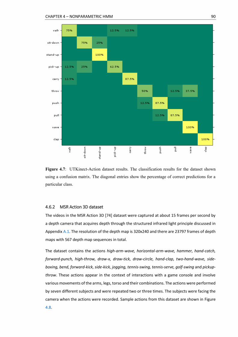
CHAPTER 4 – NONPARAMETRIC HMM 90
Figure 4.7: UTKinect-Action dataset results. The classification results for the dataset shown
using a confusion matrix. The diagonal entries show the percentage of correct predictions for a
particular class.
4.6.2 MSR Action 3D dataset
The videos in the MSR Action 3D [74] dataset were captured at about 15 frames per second by
a depth camera that acquires depth through the structured infrared light principle discussed in
Appendix A.1. The resolution of the depth map is 320x240 and there are 23797 frames of depth
maps with 567 depth map sequences in total.
The dataset contains the actions high-arm-wave, horizontal-arm-wave, hammer, hand-catch,
forward-punch, high-throw, draw-x, draw-tick, draw-circle, hand-clap, two-hand-wave, side-
boxing, bend, forward-kick, side-kick, jogging, tennis-swing, tennis-serve, golf-swing and pickup-
throw. These actions appear in the context of interactions with a game console and involve
various movements of the arms, legs, torso and their combinations. The actions were performed
by seven different subjects and were repeated two or three times. The subjects were facing the
camera when the actions were recorded. Sample actions from this dataset are shown in Figure
4.8.

CHAPTER 4 – NONPARAMETRIC HMM 91
Figure 4.8: MSR Action3D dataset samples. Actions high-arm-wave, two-hand-wave, hand-clap,
bend, golf-swing and forward-kick from the MSR Action 3D [74] dataset are shown. Top: The
depth image representation of the poses encountered when performing these actions. Bottom: The
annotated joint positions represented in a skeleton format. The circles denote the joint positions.
Figure 4.9: Feature descriptor visualization. Top: For two similar poses, the descriptor values
appear overlapped. Bottom: For two different poses, the descriptor values appear less overlapped.
As before, the information in the sequence of joint positions is used to define the features. There
are 20 joint positions in each depth frame. The relative position of a joint to all the other joints

CHAPTER 4 – NONPARAMETRIC HMM 92
in the current frame and previous frame is used in order to determine the features. Further,
instead of a single 3D coordinate vector, three 2D values representing the projection of a relative
position on the orthogonal (𝑥𝑦, 𝑦𝑧, 𝑥𝑧) Cartesian plane are used. Let the set {𝑃𝑖}𝑖=120 ∈ (𝑥, 𝑦, 𝑧)
denote the set of joint positions. For a joint 𝑖 the features are
𝑓𝑖(𝑥, 𝑦) = {(𝑃𝑖𝑥 − 𝑃𝑗
𝑥 , 𝑃𝑖𝑦
− 𝑃𝑗𝑦
) ∀ 𝑗 ∈ 𝑃(𝑡 − 1), 𝑃(𝑡), 𝑃(𝑡 + 1) ⋀ 𝑖 ≠ 𝑗}
(4.38) 𝑓𝑖(𝑦, 𝑧) = {(𝑃𝑖𝑦
− 𝑃𝑗𝑦
, 𝑃𝑖𝑧 − 𝑃𝑗
𝑧) ∀ 𝑗 ∈ 𝑃(𝑡 − 1), 𝑃(𝑡), 𝑃(𝑡 + 1) ⋀ 𝑖 ≠ 𝑗}
𝑓𝑖(𝑥, 𝑧) = {(𝑃𝑖𝑥 − 𝑃𝑗
𝑥 , 𝑃𝑖𝑧 − 𝑃𝑗
𝑧) ∀ 𝑗 ∈ 𝑃(𝑡 − 1), 𝑃(𝑡), 𝑃(𝑡 + 1) ⋀ 𝑖 ≠ 𝑗}
where 𝑃𝑖𝑥(𝑡) is the 𝑥 co-ordinate of the 𝑖𝑡ℎ joint position at time 𝑡. The gradients 𝑓𝑖(𝑥, 𝑦) are
then assigned to a histogram of 8 bins based on the direction, with the sums of gradient
magnitudes as bin values. This technique is very similar to the Histogram of Oriented Gradients
(HOG) [77]. Repeating the step for 𝑓𝑖(𝑦, 𝑧) and 𝑓𝑖(𝑥, 𝑧), there are now 24 bins for each joint.
Concatenating the bins for all the joints yields a descriptor of length 480 for every frame. Figure
4.9 provides a visualization of the feature descriptors, highlighting that for dissimilar poses the
descriptor values are different. Finally, Principle Component Analysis (PCA) [35] is used to
project the descriptor to a lower dimensional vector space. The subset of vectors that captures
at least 90% of the total variance is used.
When evaluating this dataset, the twenty actions are divided into three subsets each containing
8 actions as shown in Table 4.6. This is a common practice [11, 74] for this dataset since there
are many overlapping actions. The experiments are conducted for the challenging setting in
which the instance of a subject is not used during training and is encountered for the first time
during prediction. 60% of the subjects were used for training while the rest of the subjects were
used for testing. The parameters are initialized in the same manner described in Section 4.6.1.
Table 4.6: Actions organized into three different action sets in the MSR Action3D dataset.
Set 1 Set 2 Set 3
horizontal-arm-wave high-arm-wave high-throw
hammer hand-catch forward-kick
forward-punch draw-x side-kick
high-throw draw-tick jogging
hand-clap draw-circle tennis-swing
bend two-hand-wave tennis-serve
tennis-serve forward-kick golf-swing
pickup-throw side-boxing pickup-throw
CHAPTER 4 – NONPARAMETRIC HMM 93
The structure of the action states is explored in Figure 4.10. The action states sampled during an
iteration for the action horizontal-arm-wave are shown under A, B and C. These correspond to
different subjects for the same action. The action states for bend and pickup-throw are shown
in D and E. It can be seen that some of the states are shared across the action classes. For
instance, the state 23, which corresponds to the pose at the start and the end, is shared across
all the three classes and the state 19, which corresponds to the pose while bending, is shared by
the bend and pickup-throw actions. There are also some unique states (e.g. 9, 16 for A, 4 for B
and 7 for C) that represent the poses that are specific to these actions. This behaviour validates
the information sharing across the classes and the discriminative structure that is learnt.
The evaluation results for the MSR Action3D dataset under the full model is shown in Figure
4.11. The three confusion matrices in the figure correspond to the above three sets of actions.
As before, the diagonal entries show the percentage of correctly predicted examples. The overall
classification accuracy is 81.2% for the first set, 78.1% for the second set and 90.6% for the third
set.
Discussion
As evident from the confusion matrices, the classifier has predicted the action class labels
correctly for the most part. However, there are some misclassifications. As examples, some
bend actions are classified as pickup-throw, hand-clap actions as tennis-serve and hand-catch
actions as arm-wave. These actions involve very similar motion patterns. The draw-x and draw-
tick actions are particularly challenging to classify and have less labelling accuracy compared to
other actions.
Table 4.7 provides a summary of the classification results for this dataset. While the confusion
matrix in Figure 4.11 showed the classification accuracy for the action sets A, B and C separately,
the accuracy is pooled across all the three sets and shown in the fourth row of Table 4.7. The
behaviour of the classical HMM, nonparametric HMM and the multi-level HDP-HMM is in line
with expectations as discussed above for the UTKinect-Action dataset. The comparisons with the
other work in the literature show that the results are better than those reported in [11] and [78].
The results are less accurate when compared with the state-of-the-art results reported in [80].
The work in [80] uses the depth information in addition to the skeleton information. The depth
information is particularly useful in the MSR Action 3D dataset because there are many
corrupted joint positions. The inclusion of depth channel may benefit action recognition in this
dataset.

CHAPTER 4 – NONPARAMETRIC HMM 94
Figure 4.10: Action states. Top: The sampled action states for different instances are shown in a
colour coded plot. A, B and C correspond to the action horizontal-arm-wave while D and E
correspond to actions bend and pickup-throw, respectively. Middle: The poses corresponding to
the action states shared between the classes. Bottom: The poses corresponding to the action states
that are unique to the classes.
23 23 19 19
16 9 4 7

CHAPTER 4 – NONPARAMETRIC HMM 95
(a)
(b)
(c)

CHAPTER 4 – NONPARAMETRIC HMM 96
Figure 4.11: MSR Action 3D dataset results. The classification results for the dataset are shown
using a confusion matrix for the three different sets of action groupings. (a), (b) and (c) correspond
to Set 1, Set 2 and Set 3 respectively. The diagonal entries show the percentage of correct
predictions for a particular class.
Table 4.7: Summary of classification results for the MSR Action 3D dataset.
Method Accuracy %
This work
Parametric HMM 48.7
Nonparametric HMM 75.3
Multi-level HDP-HMM (Generative Learning) 76.8
Multi-level HDP-HMM (Discriminative Learning) 83.3
Previous Works
STIP [78] 80.8
HOJ3D [11] 78.9
JAS [80] 94.8
4.7 Conclusion
This chapter proposed a discriminative nonparametric HMM for classifying actions that occur in
depth videos. It addresses an important drawback of classical HMMs, namely the need to specify
the number of hidden states in advance. The proposed construction enables information
sharing across the action classes with the use of a single HDP-HMM. However, this single HDP-
HMM is not suitable for classification tasks. Hence the HDP-HMM is extended to include another
level that captures variations specific to each class using additional parameters. The
distributions for these parameters are formulated as transformations from a shared base
distribution. A tractable inference procedure that learns the parameters in a discriminative
manner is also provided. The construction facilitates the use of unlabelled examples and is
applicable for the classification of a wide variety of sequential data.
The experiments conducted on benchmark video datasets demonstrate the usefulness of the
proposed method in classifying human actions. The model provided here has produced good
classification results. However, there are instances in which the classification accuracy is low.
This is particularly evident for actions that involve very similar motion patterns. One mechanism
to address this problem would be to include the objects that a subject interacts with when
performing an action. This additional information would be helpful in distinguishing actions that
have similar motion trajectories. Further, the inclusion of additional information from the RGB
and depth channels may benefit the model.

CHAPTER 4 – NONPARAMETRIC HMM 97
A limitation of the HMM in general is that it cannot capture complex temporal dependencies
that are usually encountered in real-world data. For example, it is difficult to represent
sequential data that has an inherent hierarchical structure using the HMM. The model proposed
in the next chapter addresses this problem by using an extension to the HMM. It is also possible
to let each state depend on a number of previous states in an HMM. The use of these higher
order Markov chains allows the capture of long term dependency in the data. However,
inference may be more difficult in such models. The HMM uses a joint distribution over the class
labels and the observations. Directly modelling the conditional distribution of the class labels
given the observations may be more appropriate for classification problems, as discussed in
Chapter 6. In spite of these limitations, the nonparametric HMM serves as a building block for
constructing more sophisticated models.

98
5. Supervised nonparametric Hierarchical HMM
A nonparametric hierarchical HMM is proposed in this chapter for classifying human activities.
An activity is typically composed of a set of actions with an action in turn being composed of a
set of poses. The proposed model exploits this hierarchical structure inherent in the activities.
Unlike classical hierarchical HMM, the nonparametric variant described here does not require
the number of hidden states corresponding to the actions and poses to be fixed in advance. The
generic formulation proposed here is applicable for the classification of any sequential data that
exhibits a hierarchical structure.
The chapter begins with an overview of the proposed approach in Section 5.1 and is followed in
Section 5.2 by a description of the nonparametric hierarchical HMM (H-HMM). The activity
model uses a two level H-HMM with the bottom level characterizing the granular poses and the
top level characterizing the coarser actions. The relationship between the actions and the
activity labels are captured using multinomial logistic regression. Section 5.3 describes this
model structure, which is suitable for supervised classification problems. The posterior inference
procedure that ensures the alignment of actions from activities with similar labels is discussed
in Section 5.4. Experiments are conducted on depth videos to evaluate the model. The skeletal
joint positions extracted from a depth image and the information in the depth image patches
around the joint positions are used to define the features of an activity. The results for activity
classification are presented in Section 5.5. The chapter ends with some concluding remarks in
Section 5.6. Portions of this chapter have been published [194].
5.1 Overview
The action classification solution presented in the previous chapter addresses the recognition of
simple actions. However, in many situations there is a need to reason at a cognitively higher
level based on these simple actions. An activity, which is a sequence of actions, characterizes
this higher level construct. As an example, the jump, walk and run actions are part of an exercise
activity. Similarly a rinse-mouth activity is composed of drink and spit actions. We now have an
organization in which the activities are composed of actions and the actions are composed of
poses.

CHAPTER 5 – NONPARAMETRIC H-HMM 99
An additional benefit of this organization is the opportunity to share information across the
activity classes. For many actions and activities that are related, the same pose may be present
in multiple actions and the same action may be present in multiple activities. Hence it is
beneficial to share the action and pose information between the activity classes. Such
information sharing facilitates effective learning from a limited set of examples. Furthermore
the activities can now be classified just from the action representations without explicitly taking
into account the pose representations. This results in a simplified model.
The organization of an activity as a sequence of actions and an action in turn as a sequence of
poses indicates a natural hierarchical structure. The canonical Hidden Markov Model (HMM)
[32] that is widely used for representing sequential data is not sufficient to capture hierarchical
structures. There are now two levels – a top level for the coarse action sequence and a bottom
level for the granular pose sequence. Intuitively, we want an action to emit a sequence of poses
and when the action completes, it must transition to a different action which will emit a different
pose sequence. Hence for a given action state at the top level, there is a sub-HMM conditioned
on this state that emits a pose sequence. The hierarchical HMM (H-HMM) captures such a multi-
level structure by making each hidden state an autonomous probabilistic model [81]. It
generates sequences by recursively activating the sub-states of a state. In this context, when an
action state is activated, this state will use its own probabilistic model to emit a sequence of
pose states with a pose state emitting an observation. There are multiple such probabilistic
models corresponding to each action state. Although the H-HMM can be transformed into the
standard HMM by using a large number of states, the inference is easier with H-HMM for
hierarchical data. Further, the H-HMM provides a multi-scale interpretation of the data [83].
The subject performing an action often interacts with the objects in a scene. The pose
representation in the previous chapter used the information in the skeletal joint positions to
detect the actions. It may be useful to include the information about the objects as part of the
pose space. If we do so, then there are now two types of poses – the skeleton pose, which is a
particular arrangement of the joint positions and the object pose, which is a specific
representation of an object associated with the action. As an example, the drink action may
involve skeleton poses corresponding to lifting an arm and the object pose may be the
representation of a mug. In order to include the object information, the H-HMM is extended
with two independent Markov chains at the bottom level. One of the Markov chain corresponds
to the skeleton poses and the other to the object poses. This factorized representation, provides
the flexibility to include additional data channel if available in the model. The joint positions
extracted from a depth image can be used for representing the skeleton poses as discussed

CHAPTER 5 – NONPARAMETRIC H-HMM 100
earlier. The information in the depth image patches around the joint positions provides a
representation for the object poses. Figure 5.1 provides an illustration.
Figure 5.1: Activity Recognition Overview. Poses are learnt from observations and actions are
learnt from poses. S1 to S4 represent the skeleton pose states, O1 to O3 the object pose states and
A1 to A3 the action states. The skeleton poses are based on the 3D joint positions and the object
poses are based on the depth image patch around the joint positions. The same pose can be present
in multiple actions and different activities can contain the same action. The activities are classified
only based on the action states.
In the standard H-HMM, the number of action states and pose states must be specified in
advance. This is a problem in general with all variants of the classical parametric HMMs where
the number of hidden states are fixed a-priori, even though for many applications this number
is not known in advance. The usual technique of carrying out training using different choices for
the number of states is even more difficult in the case of H-HMM since there are different states
at multiple levels in the hierarchy. A better approach is to estimate the correct number of states
automatically from the data. As discussed in the previous chapters, the Hierarchical Dirichlet
Process (HDP) provides a nonparametric prior that allows an unbounded number of states to be
used. This HDP prior is applied to the different levels in the H-HMM with the cardinality of the
action and pose state space estimated from data.
In order to apply the nonparametric H-HMM for classification tasks, a separate model must be
trained individually for each class with the prediction based on the learned class conditional
density. However, it will not be possible to exploit the advantages of information sharing and
model simplification discussed above using this approach. Hence a single H-HMM is used here
with the actions and poses being shared across the activity classes. To enable classification,
S1 O1 S2 O2 O2 S3 S1 O3 S4 O3
A1 A2
Activity A
A3
Activity B

CHAPTER 5 – NONPARAMETRIC H-HMM 101
multinomial logistic regression is used to capture the relationship between the activity labels
and the actions. More specifically, the activity labels are regressed on the action states with the
regression coefficients learned using a sparsity promoting Laplacian prior [82]. When sampling
the action states during inference, the conditional likelihood of actions for a given activity label
is incorporated. This ensures that the learnt actions not only explain the observations but also
can predict the activity labels.
Contributions
The main contribution in this chapter is the definition of a novel factorized nonparametric H-
HMM model integrated with multinomial logistic regression. A tractable inference procedure
that is suitable for sequential data classification is also derived. The proposed model offers the
following advantages:
(a) The hierarchical composition of actions and poses enables information sharing and
model simplification.
(b) The nonparametric extension precludes the need for specifying a priori bounds on the
number of states.
(c) The factorized state representation allows incorporation of multiple data channels.
(d) Unlabeled examples can be used thus promoting semi-supervised learning.
(e) The model is generic and can be applied for other hierarchical sequence classification
problems.
5.2 Hierarchical HMM
In the HMM described in Section 3.1, 𝑥𝑡 denotes an observation at a time instant 𝑡 and 𝑧𝑡
denotes the corresponding state. The HMM is parameterized by the state transition probability
matrix 𝜋, where the probability of transitioning from state 𝑗 to 𝑘 is given by
𝑃(𝑧𝑡 = 𝑘|𝑧𝑡−1 = 𝑗) = 𝜋𝑗𝑘, and the state specific observation density parameters {휃𝑘}1𝐾 with 𝐾
being the number of hidden states.
In the hierarchical extension of the HMM [83], there are multiple levels 1. . . 𝑙 … 𝐿 and there is a
hidden state 𝑧𝑡𝑙 corresponding to each level 𝑙 at time 𝑡. A state at level 𝑙 emits a sequence of
states for level 𝑙 + 1 and when this state enters the end state, it activates the level above it to
emit 𝑙 − 1 level’s subsequence. Intuitively, each level has a sub-HMM conditioned on its state
with each state being a self-contained probabilistic model that is itself a hierarchical HMM.
Unlike the HMM in which the states only emit observations, the states in an H-HMM can also
emit other state sequences.

CHAPTER 5 – NONPARAMETRIC H-HMM 102
In order to indicate whether a level has completed emitting its subsequence, a binary variable
𝑓𝑡𝑙 is used. When 𝑓𝑡
𝑙 = 0, the states at all levels above 𝑙 remains unchanged. The transition to a
different state occurs horizontally within the same level. When 𝑓𝑡𝑙 = 1, the state one level above
the current level is activated. This can be interpreted as a vertical transition.
Figure 5.2: Graphical representation of a Hierarchical HMM [83]. The states at various levels,
the observations and the parameters are shown. Each dotted rectangle groups the variables at a
time instant. If the current level 𝑙 has not finished (𝑓𝑡−1𝑙 = 0), then the state 𝑧𝑡
𝑙−1 is the same state
𝑧𝑡−1𝑙−1 at the previous time 𝑡 − 1. Otherwise, its new value is determined from the state at previous
levels 𝑧𝑡1:𝑙−1. The transition parameters 𝜋1..𝐿 and emission distribution parameters 휃 are shown
on the left.
The state transition probabilities of the H-HMM need additional conditioning on the states in
the level above them. Consequently, the transition probability matrix 𝜋 must now include an
additional dimension for the hierarchical levels. The probability of transitioning to state 𝑘 from
𝑗 for level 𝑙 is now given by 𝑃(𝑧𝑡𝑙 = 𝑘 | 𝑧𝑡−1
𝑙 = 𝑗, 𝑧𝑡1..𝑙−1 = 𝑖) = 𝜋𝑗,𝑘
𝑙 where 𝑖 is the current state
corresponding to all the parent levels 𝑧𝑡1..𝑙−1. Let the conditional probability of the binary
variables when the level below has completed be 𝑃(𝑓𝑡𝑙 = 1 |𝑓𝑡
𝑙+1 = 1, 𝑧𝑡𝑙 , 𝑧𝑡
𝑙−1) = 𝜓𝑙,𝑧𝑡𝑙,𝑧𝑡
𝑙−1.
Here each 𝜓 is a parameter that controls the probability of a state transition at a particular level.
Finally, it is common to assume that the states that emit the observations are at the bottom
level and hence the state specific observation density parameters remain identical to the HMM.
A graphical representation is provided in Figure 5.2.
𝑧11
𝑥1
...
𝑧1𝐿
...
𝑧12
𝑓12
𝑓11
𝑓1𝐿
𝑧21
𝑥2
𝑧2𝐿
...
𝑧22 ...
𝑧𝑇1
𝑓𝑇1
𝑧𝑇2
𝑓𝑇2
𝑧𝑇𝐿
...
𝑓𝑇2
𝑥𝑇
𝜋𝑗1
𝐾
𝜋𝑗2
𝐾
𝜋𝑗𝐿
𝐾
휃𝑘
𝐾
...
...
𝑓21
𝑓22
𝑓2𝐿
...

CHAPTER 5 – NONPARAMETRIC H-HMM 103
Nonparametric variant
In order to construct the nonparametric variant of the H-HMM, it is useful to define the Bayesian
extension first by introducing priors for the parameters. Similar to the Bayesian HMM described
in Section 4.2, the rows of the transition matrix must be coupled. Let the priors be
𝛽𝑙 ~ 𝐷𝑖𝑟(𝛾
𝐾…
𝛾
𝐾) and 𝜋𝑗
𝑙 ~ 𝐷𝑖𝑟(𝛼𝛽1𝑙 … 𝛼𝛽𝐾
𝑙 ) where 𝐷𝑖𝑟 is the Dirichlet distribution, 𝐾 is the
number of states and 𝛾, 𝛼 are some positive real numbers. Note that the Dirichlet priors are now
extended to multiple levels 𝛽1:𝐿 and 𝜋𝑗1:𝐿 when compared with HMM. The 𝜓 parameters can be
assigned a Beta prior 𝐵𝑒𝑡𝑎(𝑎, 𝑏) where 𝑎, 𝑏 ∈ ℝ+. Let us also assign the observation density
parameters a prior 𝐻 with the exact form of this prior depending on the parameters themselves.
With this definition, an observation is generated in the Bayesian H-HMM as follows:
𝛽𝑙 | 𝛾 ~ 𝐷𝑖𝑟 (𝛾
𝐾) 𝑙 = 1, … 𝐿 (5.1)
𝜋𝑗𝑙 | 𝛼, 𝛽𝑙 ~ 𝐷𝑖𝑟(𝛼𝛽1
𝑙 … 𝛼𝛽𝐾𝑙 )
𝑗 = 1, … 𝐾
𝑙 = 1, … 𝐿 (5.2)
𝜓𝑙,𝑘,𝑘′ | 𝑎, 𝑏 ~ 𝐵𝑒𝑡𝑎(𝑎, 𝑏)
𝑙 = 1, … 𝐿
𝑘, 𝑘′ = 1. . 𝐾 (5.3)
휃𝑘 | 𝐻 ~ 𝐻 𝑘 = 1, … 𝐾 (5.4)
𝑧𝑡𝑙 | 𝑧𝑡−1
1:𝑙 , 𝑓𝑡−11:𝑙 , 𝜋 ~ {
𝜋𝑧𝑡−1
𝑙𝑙 𝑖𝑓 𝑓𝑡−1
𝑙 = 0
𝜋0,𝑧𝑡
𝑙−1𝑙−1 𝑜𝑡ℎ𝑒𝑟𝑤𝑖𝑠𝑒
𝑡 = 1, … . 𝑇 (5.5)
𝑥𝑡 | 𝑧𝑡𝐿 , {휃𝑘}𝑘=1
∞ ~ 𝐹(휃𝑧𝑡𝐿) 𝑡 = 1, … 𝑇 (5.6)
If each level of the H-HMM is considered separately, then the generation process in (5.1) and
(5.2) is similar to the process by which the observations are generated using HDP and the
nonparametric HMM. The 𝜋𝑗 distributions in the HDP are similar to the 𝜋𝑗𝑙 distributions in the H-
HMM. By assigning independent HDP priors to the different levels of the H-HMM, a
nonparametric variant of the H-HMM is obtained. The number of states in each level is
unbounded and the equations (5.1) and (5.2) with the HDP prior are written as
𝛽𝑙 | 𝛾 ~ 𝐺𝐸𝑀(𝛾) 𝑙 = 1, … 𝐿 (5.7)
𝜋𝑗𝑙 | 𝛼, 𝛽𝑙 ~ 𝐷𝑃(𝛼, 𝛽𝑙)
𝑗 = 1,2, …
𝑙 = 1, … 𝐿 (5.8)
The rest of the generative process in (5.3) to (5.6) remains the same except that 𝐾 is unbounded.
Note that in an alternative construction, the number of levels 𝐿 in the H-HMM can be

CHAPTER 5 – NONPARAMETRIC H-HMM 104
unbounded [84]. This is not considered here since the number of hierarchical levels is known a-
priori in this context.
5.3 Activity Model
Let i.i.d training data 𝑋 = {𝑥𝑛}𝑛=1𝑁 , 𝑌 = {𝑦𝑛}𝑛=1
𝑁 be given. Here 𝑥𝑛 = 𝑥1𝑛 … 𝑥𝑇
𝑛 is an
observation sequence and 𝑦𝑛 ∈ { 1 … 𝑐 … 𝐶} is the class label corresponding to the observation
𝑥𝑛. For example, in activity classification, 𝑥𝑛 is the input image sequence and 𝑦𝑛 is the activity
class label. At a time instant 𝑡, the activity observation 𝑥𝑡 contains a factored set of features.
There are two types of features – the skeleton features 𝑥𝑠𝑡 ∈ ℝ𝑑𝑠 that represent the
information about the joint positions and the object features 𝑥𝑜𝑡 ∈ ℝ𝑑𝑜 that represent an
object. Let 𝑥𝑡 = (𝑥𝑠𝑡, 𝑥𝑜𝑡). Further discussion of the features is deferred to Section 5.5. The
objective is classification: given a new test activity sequence 𝑥, the corresponding activity label
�̂� must be predicted using the information learned when training the model. A suitable
prediction is
�̂� = argmax𝑐
𝑝(𝑐 | 𝑥, 𝑋, 𝑌) (5.9)
5.3.1 Structure
The H-HMM model structure proposed here differs from the canonical H-HMM in three key
aspects. Firstly, the number of levels is restricted to two. This simplified model with only two
levels ensures tractable inference, while retaining the benefits of a compact hierarchical
structure. Secondly, a factored form of the states is presented, which provides flexibility to add
new data channels if necessary. Finally, unlike H-HMM, the output label corresponding to the
input activity is integrated directly into the model structure.
The top level contains the action states that emit the pose state sequence. Let 𝑎𝑡 be the hidden
action state at time 𝑡. The bottom level contains the pose states which in turn emit the
observations. A pose state at time 𝑡 is factored into two different discrete states – a skeleton
state 𝑧𝑠𝑡 and an object state 𝑧𝑜𝑡. The action, skeleton pose and object pose have separate HDP
priors and there is no a priori upper bound on the number of states.
A single binary variable 𝑓𝑡 is used to indicate whether an action state has completed or not. If
the binary variable has a zero value, then the action states remain unchanged and a new pose
state is determined based on the pose state at previous time instant. Otherwise, there is a
transition to a new action state. The single indicator variable controls the transition of the
bottom level states and the action states.

CHAPTER 5 – NONPARAMETRIC H-HMM 105
The pose states always emit a single observation. Each observation consists of two samples from
independent Gaussian distributions - one for the skeleton pose and the other for the object
pose. Given a skeleton pose state 𝑘, the skeleton observations are drawn from 𝒩(𝜇𝑠𝑘, Σs𝑘).
Similarly, the object observations are drawn from 𝒩(𝜇𝑜𝑘 , Σo𝑘) for an object pose state 𝑘. The
observations are independent of the action state given the pose state. The density parameters
are assigned appropriate priors. For example, the mean parameters have independent normal
priors and the covariance parameters have independent Inverse-Wishart priors.
In order to perform classification, an activity label is modelled by multinomial logistic regression
[16] conditioned on the assignment of action states. Let 𝑎 be a vector that represents the
number of transitions from one action state to another in an unknown activity. Let the set of all
regression coefficients be 𝜼 = [휂1 … 휂𝐶] where 휂𝑐 are the coefficients corresponding to the
activity class 𝑐. The linear predictor for a label is then computed as 휂𝑐⊺𝑎. Intuitively, the
parameter space is now extended to include the linear predictor and during inference, as
explained in Section 5.4, the regression coefficients influence the action states and vice-versa.
This ensures that the activities can be discriminated from one another based on the assignment
of action states. The labels do not depend directly on the skeleton and object pose states.
Figure 5.3: Graphical representation of the activity Model. The top level contains action states
𝑎1:𝑇 that emit the bottom level skeleton pose 𝑧𝑠1:𝑇 and object pose 𝑧𝑜1:𝑇 states which in turn emit
the observations 𝑥1:𝑇. The binary variable 𝑓𝑡 determines whether the action state remains
unchanged or not. The action states determine the activity label 𝑦. The parameters and their priors
are in the left side. This representation differs from the standard H-HMM in three ways: (i) the
integration of label 𝑦, (ii) the factored form of 𝑥 and 𝑧 and (iii) the presence of the priors.
𝑧𝑠1
𝑎1 𝑎2
𝑧𝑜1
𝑧𝑠2
𝑧𝑜2
𝑥𝑠1
𝑥𝑜1
𝑥𝑠2
𝑥𝑜2
... 𝑧𝑠𝑇
𝑎𝑇
𝑧𝑜𝑇
𝑥𝑠𝑇
𝑥𝑜𝑇
...
...
𝑓1
𝑓2
𝑓𝑇
𝛽
𝜋𝑗
∞
𝜓𝑘
∞
𝜑𝑠𝑜𝑗
∞
𝜇, Σ𝑘
∞
𝜌𝑠𝑜
𝛾
𝛼
𝜚
𝜏
𝐻
𝜅
𝑦 휂 𝜆

CHAPTER 5 – NONPARAMETRIC H-HMM 106
5.3.2 Generative Process
Following the above model, the generation process for an observation is summarized as follows.
First the priors are drawn from their hyper priors in steps 1 to 5 and then the observations are
drawn according to steps 6 to 12. Figure 5.3 provides an overview.
1) Draw the HDP priors for the top level action states from the hyper parameters. Let 𝛽 be
the overall distribution for the action states, and let 𝜋𝑗 be the set of transition
probabilities.
𝛽 | 𝛾 ~ 𝐺𝐸𝑀(𝛾)
𝜋𝑗 | 𝛼, 𝛽 ~ 𝐷𝑃(𝛼, 𝛽) 𝑗 = 1,2, … (5.10)
2) Draw the HDP priors for the bottom level states from the hyper parameters. This
includes both the skeleton pose states and object pose states. Note that for each action
state, there is a set of skeleton states and a set of object states. Given an action state 𝑎,
let 𝜌𝑠𝑎 be the overall distribution of skeleton states and let 𝜑𝑠𝑗𝑎 be the distribution for
the 𝑗𝑡ℎ skeleton state. Similarly, let 𝜌𝑜𝑎 be the overall distribution of object states and
let 𝜑𝑜𝑗𝑎 be the distribution for the 𝑗𝑡ℎ object state.
𝜌𝑠𝑎| 𝜚 ~ 𝐺𝐸𝑀(𝜚) 𝑎 = 1,2, …
𝜌𝑜𝑎| 𝜚 ~ 𝐺𝐸𝑀(𝜚) 𝑎 = 1,2, …
𝜑𝑠𝑗𝑎| 𝜏, 𝑎, 𝜌𝑠𝑎 ~ 𝐷𝑃(𝜏, 𝜌𝑠𝑎) 𝑗 = 1,2, …
𝜑𝑜𝑗𝑎| 𝜏, 𝑎, 𝜌𝑜𝑎 ~ 𝐷𝑃(𝜏, 𝜌𝑜𝑎) 𝑗 = 1,2, …
(5.11)
3) Draw the normal distribution mean and covariance parameters from the hyper
parameters. The skeleton pose parameters are 𝜇𝑠, Σs and object pose parameters are
𝜇𝑜, Σo respectively. The hyper-parameters 𝜇0, Σ0 correspond to the mean and
covariance of the normal prior and the hyper-parameters 𝜈0, Δ0 correspond to the
Inverse-Wishart prior.
𝜇𝑠𝑘 | 𝜇0𝑠 , Σ0
𝑠 ~ 𝒩(𝜇0𝑠 , Σ0
𝑠) 𝑘 = 1,2, …
Σs𝑘 | 𝜈0𝑠, Δ0
𝑠 ~ 𝐼𝑊(𝜈0𝑠, Δ0
𝑠 ) 𝑘 = 1,2, …
𝜇𝑜𝑘 | 𝜇0𝑜, Σ0
𝑜 ~ 𝒩(𝜇0𝑜, Σ0
𝑜) 𝑘 = 1,2, …
Σo𝑘 | 𝜈0𝑜, Δ0
𝑜 ~ 𝐼𝑊(𝜈0𝑜, Δ0
𝑜) 𝑘 = 1,2, …
(5.12)
4) Draw the Bernoulli priors from which the completion indicator variables are drawn.
𝜓𝑎,𝑘𝑠,𝑘𝑜 | 𝜅𝑎, 𝜅𝑏 ~ 𝐵𝑒𝑡𝑎(𝜅𝑎, 𝜅𝑏) 𝑎, 𝑘𝑠, 𝑘𝑜 = 1,2, … (5.13)

CHAPTER 5 – NONPARAMETRIC H-HMM 107
5) Draw the regression coefficients for all the classes from a Laplacian prior. Let ||𝜼||1
denote the 𝑙1 norm. The Laplacian prior is given as follows with 𝜆 being a hyper-
parameter.
𝜼 | 𝜆 ~ exp(−𝜆||𝜼||1) (5.14)
6) Repeat steps 7 to 12 for each observation 𝑛 and steps 7 to 11 for each time instant 𝑡 of
the observation.
7) Draw the action state from 𝜋 if the binary variable at previous time instant is on.
Otherwise, the action states remain unchanged.
𝑎𝑡𝑛 | 𝑎𝑡−1
𝑛 , 𝑓𝑡−1𝑛 , 𝜋 {
~ 𝜋𝑎𝑡−1𝑛 𝑖𝑓 𝑓𝑡−1
𝑛 = 1
= 𝛿(𝑎𝑡𝑛, 𝑎𝑡−1
𝑛 ) 𝑜𝑡ℎ𝑒𝑟𝑤𝑖𝑠𝑒 (5.15)
8) Draw the skeleton pose state from 𝜑𝑠. If the binary variable at the previous time instant
is on, which indicates that a new action state has begun, then the pose state is drawn
from an initial distribution indicated with subscript 0.
𝑧𝑠𝑡𝑛 | 𝑎𝑡
𝑛, 𝑓𝑡−1𝑛 , 𝜑𝑠 ~ {
𝜑𝑠0𝑎𝑡
𝑛
𝑖𝑓 𝑓𝑡−1𝑛 = 1
𝜑𝑠𝑧𝑠𝑡−1
𝑛𝑎𝑡
𝑛
𝑜𝑡ℎ𝑒𝑟𝑤𝑖𝑠𝑒 (5.16)
9) Draw the object pose state similarly from 𝜑𝑜. As above, if the binary variable at the
previous time instant is on, then the pose state is drawn from an initial distribution.
𝑧𝑜𝑡𝑛 | 𝑎𝑡
𝑛, 𝑓𝑡−1𝑛 , 𝜑𝑜 ~ {
𝜑𝑜0𝑎𝑡
𝑛
𝑖𝑓 𝑓𝑡−1𝑛 = 1
𝜑𝑜𝑧𝑜𝑡−1
𝑛𝑎𝑡
𝑛
𝑜𝑡ℎ𝑒𝑟𝑤𝑖𝑠𝑒 (5.17)
10) Draw the binary variable from its prior shown in step 4.
𝑓𝑡𝑛 | 𝑎𝑡
𝑛, 𝑧𝑠𝑡𝑛, 𝑧𝑜𝑡
𝑛 𝜓 ~ 𝐵𝑒𝑟(𝜓𝑎𝑡𝑛,𝑧𝑠𝑡
𝑛,𝑧𝑜𝑡𝑛
) (5.18)
11) Draw the skeleton and object observations from the normal distribution using the mean
and covariance parameters drawn according to (5.12).
𝑥𝑠𝑡𝑛 | 𝑧𝑠𝑡
𝑛, 𝜇𝑠, Σs ~ 𝒩(𝜇𝑠𝑧𝑠𝑡𝑛 , Σs𝑧𝑠𝑡
𝑛)
𝑥𝑜𝑡𝑛 | 𝑧𝑜𝑡
𝑛, 𝜇𝑜, Σo ~ 𝒩(𝜇𝑜𝑧𝑜𝑡𝑛 , Σo𝑧𝑜𝑡
𝑛) (5.19)

CHAPTER 5 – NONPARAMETRIC H-HMM 108
12) Finally draw the activity label from a multinomial distribution based on the linear
predictor. The linear predictor is computed from the action states drawn according to
(5.15) and the regression coefficients are drawn according to (5.14).
𝑦𝑛 | 𝑎1..𝑇𝑛 , 𝜼 ~ 𝑀𝑢𝑙𝑡 (
exp (휂1⊺𝑎)
∑ exp (휂𝑐′ ⊺𝑎)𝐶
𝑐′=1
…exp (휂𝐶 ⊺
𝑎)
∑ exp (휂𝑐′ ⊺𝑎)𝐶
𝑐′=1
) (5.20)
Due to the clustering nature of HDP, some observations, across activity labels, may be assigned
the same pose states. For example, two different observations that involve push and pull actions
may contain very similar alignment of skeletal joints during the course of the action. As a result,
the set of pose states for these actions could be identical. This reduces the overall number of
pose states necessary for describing all observations and promotes parameter sharing across
the labels. By extension, two different activity labels may also share the same action states if
they involve a similar sequence of pose states. Thus the model enables a reduction in the
numbers of action and pose states. The sequence of action states assigned to the observations
is sufficient for distinguishing the activities. The structure of the model is simplified by removing
the direct dependency of the activities on the observations.
5.4 Posterior Inference
Exact posterior inference is intractable in DP based models and an approximate inference
technique such as Markov Chain Monte Carlo (MCMC) must be used. The Gibbs sampling
procedure discussed in Appendix E.2 is applied here to draw posterior samples for all the
variables. The Gibbs sampler proceeds by sampling the hidden state sequence variables
assuming that the parameter variables are given and then sampling the parameter variables
assuming the hidden state sequences are available. This process is repeated for a number of
iterations until convergence. Table 5.1 lists the inference steps.
The parameter variables are 𝜋, 𝜑𝑠, 𝜑𝑜 (the transition parameters for action, skeleton and object
states), 𝜇𝑠, Σs, 𝜇𝑜, Σo (the normal distribution parameters for skeleton and object), 𝜓 (the
Bernoulli parameter for finish variable) and 𝜼 (the regression coefficients). The state sequences
are 𝑎1:𝑇 (action), 𝑧𝑠1:𝑇 (skeleton pose), 𝑧𝑜1:𝑇 (object pose) and 𝑓1:𝑇 (action completion
indicators).
5.4.1 Sampling Hidden State Sequence
Many DP based models sample one state at a time, given all other state assignments. This
method marginalizes over the unbounded number of state transitions. Sequentially sampling a
state conditioned on the states at other time instants can lead to slow mixing rates because of

CHAPTER 5 – NONPARAMETRIC H-HMM 109
the temporal correlations. Instead of this collapsed sampling procedure, it is better to explicitly
instantiate all the parameters and block sample the state sequence based on the standard belief
propagation techniques used in Bayesian networks.
The hidden states cannot be block sampled without resorting to some truncated approximation
[71]. An effective way to approximate the countably infinite hidden states is to use the weak
limit approximation to DP [76] discussed in Section 4.5.1. In this approximation, the number of
expected components is set to a large value. As this value increases without limit, the model’s
marginal distribution approaches the DP. Specifically, the stick breaking weights are
approximated as
𝐺𝐸𝑀(𝛾) ≜ 𝐷𝑖𝑟(𝛾
𝐾, …
𝛾
𝐾) (5.21)
where 𝐾 is a number that exceeds the expected number of components. The DP prior ensures
that only a small subset of the 𝐾 components is used. This truncated approximation is
computationally efficient and allows the use of existing well-studied Bayesian message passing
techniques [76]. Consequent to this approximation, equations (5.10) and (5.11) become the
following.
𝛽 | 𝛾 ~ 𝐷𝑖𝑟(𝛾
𝐾𝑎…
𝛾
𝐾𝑎)
(5.22)
𝜋𝑗 | 𝛼, 𝛽 ~ 𝐷𝑖𝑟(𝛼𝛽1, … , 𝛼𝛽𝐾𝑎 ) 𝑗 = 1, … , 𝐾𝑎
𝜌𝑠𝑎| 𝜚 ~ 𝐷𝑖𝑟(𝜚
𝐾𝑠…
𝜚
𝐾𝑠) 𝑎 = 1, … , 𝐾𝑎
𝜑𝑠𝑗𝑎| 𝜏, 𝑎, 𝜌𝑠𝑎 ~ 𝐷𝑖𝑟(𝜏𝜌𝑠1
𝑎 , … , 𝜏𝜌𝑠𝐾𝑠𝑎 )
𝑗 = 1, … , 𝐾𝑠
𝑎 = 1, … , 𝐾𝑎
𝜌𝑜𝑎| 𝜚 ~ 𝐷𝑖𝑟(𝜚
𝐾𝑜…
𝜚
𝐾𝑜)
𝜑𝑜𝑗𝑎| 𝜏, 𝑎, 𝜌𝑜𝑎 ~ 𝐷𝑖𝑟(𝜏𝜌𝑜1
𝑎 , … , 𝜏𝜌𝑜𝐾𝑜𝑎 )
𝑗 = 1, … , 𝐾𝑜
𝑎 = 1, … , 𝐾𝑎
Here 𝐾𝑎, 𝐾𝑠 and 𝐾𝑜 are the maximum number of states corresponding to action, skeleton and
object respectively. Typically the maximum number of action states is set smaller than that of
skeleton and object states. The joint distribution of an observation, its label and the state
sequence, given the parameter variables are provided as follows.

CHAPTER 5 – NONPARAMETRIC H-HMM 110
𝑝(𝑥𝑠1:𝑇 , 𝑥𝑜1:𝑇 , 𝑦, 𝑎1:𝑇, 𝑧𝑠1:𝑇 , 𝑧𝑜1:𝑇 , 𝑓1:𝑇| 𝜋, 𝜑𝑠, 𝜑𝑜, 𝜇𝑠, Σs, 𝜇𝑜, Σo, 𝜓, 𝜼)
= 𝑝(𝑦|𝑎1:𝑇) ∏ 𝑝(𝑎𝑡|𝑎𝑡−1, 𝑓𝑡−1)
𝑇
𝑡=1
𝑝(𝑧𝑠𝑡|𝑧𝑠𝑡−1, 𝑎𝑡 , 𝑓𝑡−1) 𝑝(𝑧𝑜𝑡|𝑧𝑜𝑡−1, 𝑎𝑡 , 𝑓𝑡−1)
𝑝(𝑓𝑡|𝑎𝑡 , 𝑧𝑠𝑡, 𝑧𝑜𝑡) 𝑝(𝑥𝑠𝑡|𝑧𝑠𝑡) 𝑝(𝑥𝑜𝑡|𝑧𝑜𝑡)
(5.23)
A key challenge is to ensure that when sampling at time 𝑡, the action state 𝑎𝑡, skeleton state
𝑧𝑠𝑡, object state 𝑧𝑜𝑡 and the binary variable 𝑓𝑡 are block sampled together. It is essential to
perform efficient message passing inference similar to the dynamic programming algorithm of
Section 3.1.1 used in HMMs for convergence. In order to achieve this efficiency, the H-HMM is
flattened and all possible combinations of these variables are considered. This flattening might
not be practical if there are too many states at the various levels of the hierarchy. However, the
number of possible states is bounded here by the use of a truncated DP. The flattening and the
weak limit approximation in (5.22), allows the use of variations of the forward-backward
algorithm to sample the state sequence.
There is no straight forward mechanism available to include the conditional likelihood term
𝑝(𝑦|𝑎1:𝑇) while block sampling the posterior states using the forward-backward algorithm. This
likelihood is approximated by using the action state sequence sampled from a previous iteration.
Let 𝒂 be a sampled action state sequence corresponding to an observation sequence in a
previous sampling iteration.
Let 𝑉(. ) be an intermediate term that represents the joint probability for being in a specific
combination of states and emitting an observation given another set of states.
𝑉(. ) = 𝑃(𝑎𝑚 = 𝑘𝑎, 𝑧𝑠𝑚 = 𝑘𝑠, 𝑧𝑜𝑚 = 𝑘𝑜, 𝑓𝑚−1 = 𝑓′, 𝑥𝑠𝑚, 𝑥𝑜𝑚, 𝑦|
𝑎𝑛 = 𝑘𝑎′, 𝑧𝑠𝑛 = 𝑘𝑠′
, 𝑧𝑜𝑛 = 𝑘𝑜′, 𝑓𝑛 = 𝑓′′
)
𝑚, 𝑛
∈ {1. . . 𝑇} (5.24)
Using the factorization of the joint distribution in (5.23), and substituting the terms from
equations (5.15) to (5.20), 𝑉(. ) can be written as
𝑉(𝑘𝑎 , 𝑘𝑠, 𝑘𝑜, 𝑓′, 𝑥𝑠𝑡, 𝑥𝑜𝑡, 𝑦 | 𝑘𝑎′, 𝑘𝑠′
, 𝑘𝑜′, 𝑓′′
, 𝜼, 𝒂) =
[[𝛿(𝑓′′, 1) 𝜋
𝑘𝑎′,𝑘𝑎 𝜑𝑠0,𝑘𝑠
𝑘𝑎 𝜑𝑜0,𝑘𝑜
𝑘𝑎] + [𝛿(𝑓′′
, 0) 𝛿(𝑘𝑎, 𝑘𝑎′) 𝜑𝑠
𝑘𝑠′,𝑘𝑠
𝑘𝑎 𝜑𝑜
𝑘𝑜′,𝑘𝑜
𝑘𝑎]]
𝐵𝑒𝑟(𝑓′; 𝜓𝑘𝑎,𝑘𝑠,𝑘𝑜) 𝒩(𝑥𝑠𝑡; 𝜇𝑠𝑘𝑠 , Σs𝑘𝑠) 𝒩(𝑥𝑜𝑡; 𝜇𝑜𝑘𝑜 , Σo𝑘𝑜)
exp(𝜂𝑦⊺𝑎)
∑ exp(𝜂𝑐′⊺𝑎)𝐶
𝑐′=1
(5.25)
In the above, 𝛿 is the Kronecker Delta function with 𝛿(𝑚, 𝑛) = 1, if 𝑚 = 𝑛 . The second line
represents the probability of transitioning from 𝑘𝑎′ to 𝑘𝑎, 𝑘𝑠′
to 𝑘𝑠 and 𝑘𝑜′ to 𝑘𝑜, all together,
for a binary variable with value 𝑓′′. The third line represents the 𝑓′ probability, observations

CHAPTER 5 – NONPARAMETRIC H-HMM 111
probability and the label probability for a particular state sequence. The term 𝑎 is computed
from 𝒂.
In order to block sample the states, messages passed backwards in time from 𝑡 = 𝑇 … 1 and
forward from 𝑡 = 1 … 𝑇 are used. The forward and backward messages in a standard HMM are
computed recursively from the probability of transitioning from one state to another and the
probability of emitting an observation. Here there are three different state variables 𝑎𝑡, 𝑧𝑠𝑡 and
𝑧𝑜𝑡 and also a finish variable 𝑓𝑡−1 on which the state transitions are conditioned upon. The
observation likelihood now includes the 𝑥𝑠𝑡 and 𝑥𝑜𝑡 terms, in addition to the label likelihood.
The 𝑉(. ) term represents these probabilities and it can be used to compute the forward and
backward messages. The forward message 𝑚𝑡−1,𝑡, which represents the joint probability of
states at time 𝑡 and the observations up to time 𝑡, is computed recursively as follows:
𝑚𝑡−1,𝑡(𝑘𝑎, 𝑘𝑠, 𝑘𝑜, 𝑓′|𝑥𝑠1:𝑇 , 𝑥𝑜1:𝑇, 𝑦, 𝜼, 𝒂) =
∑ ∑ ∑ ∑ 𝑚𝑡−2,𝑡−1(𝑘𝑎′, 𝑘𝑠′
, 𝑘𝑜′, 𝑓′′
|𝑥𝑠1:𝑇, 𝑥𝑜1:𝑇 , 𝑦, 𝜼, 𝒂)
𝑓′′∈{0,1}𝑘𝑜′
∈ 𝐾𝑜𝑘𝑠′∈ 𝐾𝑠𝑘𝑎′
∈ 𝐾𝑎
𝑉(𝑘𝑎, 𝑘𝑠, 𝑘𝑜, 𝑓′|𝑘𝑎′, 𝑘𝑠′
, 𝑘𝑜′, 𝑓′′
, 𝑥𝑠𝑡, 𝑥𝑜𝑡 , 𝑦, 𝜼, 𝒂)
(5.26)
The backward message 𝑚𝑡,𝑡−1 is the message that is passed from time 𝑡 to 𝑡 − 1 with 𝑚𝑇+1,𝑇 =
1. It represents the probability of observing states in the future from a current state. The
backward message is also based on the probability of state transitions and the observation
probability, which the 𝑉 term represents. The backward message is determined recursively over
all possible states as follows.
𝑚𝑡,𝑡−1(𝑘𝑎, 𝑘𝑠, 𝑘𝑜, 𝑓′|𝑥𝑠1:𝑇 , 𝑥𝑜1:𝑇, 𝑦, 𝜼, 𝒂) =
∑ ∑ ∑ ∑ 𝑚𝑡+1,𝑡(𝑘𝑎′, 𝑘𝑠′
, 𝑘𝑜′, 𝑓′′
|𝑥𝑠1:𝑇 , 𝑥𝑜1:𝑇 , 𝑦, 𝜼, 𝒂)
𝑓′′∈{0,1}𝑘𝑜′
∈ 𝐾𝑜𝑘𝑠′∈ 𝐾𝑠𝑘𝑎′
∈ 𝐾𝑎
𝑉(𝑘𝑎′, 𝑘𝑠′
, 𝑘𝑜′, 𝑓′′
|𝑘𝑎, 𝑘𝑠, 𝑘𝑜, 𝑓′, 𝑥𝑠𝑡, 𝑥𝑜𝑡 , 𝑦, 𝜼, 𝒂)
(5.27)
The conditional distribution of the states given the observations is a product of the forward
and backward messages. The states are sampled from this conditional distribution. Let 𝒂−𝑡
denote the terms excluding the 𝑡𝑡ℎ term with 𝒂 = 𝒂−𝑡 + (𝑎𝑡 = 𝑘𝑎) for some action state 𝑘𝑎.
Using the forward and backward messages, the hidden state at time 𝑡 is sampled as below.
CHAPTER 5 – NONPARAMETRIC H-HMM 112
𝑝(𝑎𝑡 = 𝑘𝑎, 𝑧𝑠𝑡 = 𝑘𝑠, 𝑧𝑜𝑡 = 𝑘𝑜, 𝑓𝑡 = 𝑓′ |𝑥𝑠1:𝑇 , 𝑥𝑜1:𝑇, 𝑦, 𝜼, 𝒂) ∝
𝑚𝑡+1,𝑡(𝑘𝑎, 𝑘𝑠, 𝑘𝑜, 𝑓′|𝑥𝑠1:𝑇, 𝑥𝑜1:𝑇 , 𝑦, 𝜼, 𝒂) ×
𝑚𝑡−1,𝑡(𝑘𝑎, 𝑘𝑠, 𝑘𝑜, 𝑓′|𝑥𝑠1:𝑇 , 𝑥𝑜1:𝑇 , 𝑦, 𝜼, 𝒂−𝑡 + 𝑘𝑎)
(5.28)
5.4.2 Sampling Parameters
The sampled state sequences are used to compute count matrices. Each element in the matrix
records the number of transitions from one state to another. Let 𝐴 ∈ ℤ(𝐾𝑎+1)×𝐾𝑎 be a matrix of
counts computed from the sampled action state sequences with 𝐴𝑗𝑘 being the number of
transitions from action state 𝑗 to 𝑘 across the training set. The number of transitions for an initial
action state 𝐴0𝑘is maintained in the 𝐾𝑎 + 1 row. Similarly, let 𝑆𝑎 ∈ ℤ(𝐾𝑠+1)×𝐾𝑠 and 𝑂𝑎 ∈
ℤ(𝐾𝑜+1)×𝐾𝑜 be the count matrices corresponding to the skeleton and object states for an action
𝑎. The HDP transition parameters 𝛽, 𝜌𝑠, 𝜑𝑠, 𝜌𝑜, 𝜑𝑜 and their hyper parameters can be sampled
from their posteriors, one at a time, through standard inference methods [44] using these count
matrices. The notable exception is for action state transition parameter 𝜋 for which it is
preferable to disable self-transitions 𝜋𝑗𝑗 since 𝑓𝑡 = 0 already implies that 𝑎𝑡 = 𝑎𝑡+1. The data
augmentation procedure in [92] is followed to resample 𝜋.
Let 𝐹𝑘𝑎,𝑘𝑠,𝑘𝑜∈ ℤ be the number of times an action, skeleton and object state combination is in
a completed state. This value can be computed from the sampled 𝑓1:𝑇 values. The Bernoulli
variable 𝜓 has a conjugate Beta prior and the posterior updates can be performed analytically
using the computed 𝐹𝑘𝑎,𝑘𝑠,𝑘𝑜 values as discussed in Appendix C.3.
In order to sample the Normal distribution parameters, the sampled state sequences are used
again. Let the set of skeleton observations assigned to hidden state 𝑘𝑠 be 𝒳𝑆𝑘𝑠 = {𝑥𝑠𝑡𝑛 ∈ 𝑋 ∶
𝑧𝑠𝑡𝑛 = 𝑘𝑠}. The mean and covariance parameters have conjugate priors and hence a closed
form posterior update for 𝜇𝑠𝑘𝑠 , Σs𝑘𝑠 can be directly computed based on the set 𝒳𝑆𝑘𝑠 as seen in
the previous chapters. A similar procedure is followed for the object pose mean and covariance
parameters. The term 𝑎 can be computed from the action state sequence 𝒂 for (5.24) or from
any 𝑎1:𝑇 in general. For example, if 𝑎𝑡 is represented as a 𝐾 length vector, with an element 𝑘
being 1 when 𝑎𝑡 = 𝑘 and 0 otherwise, then 𝑎 =1
𝑇∑ 𝑎𝑡𝑡 . Alternatively, 𝑎 can represent the
number of transitions from one action state to another.
This leaves only the estimation of regression coefficients 𝜼. Using a Laplacian prior for 𝜼 rather
than a normal prior on the coefficients encourages coefficient values which are either relatively
large or near to zero. The sparseness of this prior leads to structural simplification and often
results in generalization and better classification results [93]. The sparse multinomial logistic

CHAPTER 5 – NONPARAMETRIC H-HMM 113
regression [82] provides a fast exact algorithm that scales favourably as the dimension of the
features increases. The algorithm can be applied to large data sets in high dimensional feature
spaces. This procedure is used here for estimating the regression weights .
5.4.3 Prediction
During prediction, a test activity sequence’s label is determined. In order to do this, first the
action state sequence is inferred using Viterbi decoding, discussed in Section 3.1.1, from the
parameters corresponding to a posterior sample. The conditional likelihood term in (5.23) is not
used in this process. The linear predictor is then determined from the regression coefficients 휂
and 𝑎, where 𝑎 is computed from the inferred action state sequence. The label is obtained using
(5.29).
�̂� = argmax𝑐
exp (휂𝑐⊺𝑎)
∑ exp (휂𝑐′ ⊺𝑎)𝐶
𝑐′=1
= argmax𝑐
exp (휂𝑐⊺𝑎)
(5.29)
Table 5.1: Posterior Inference Algorithm
Input: Training examples of activity sequences with their corresponding labels.
Output: Samples of posterior parameters.
1. Sample initial values of 𝛽, 𝜋, 𝜌𝑠, 𝜑𝑠, 𝜌𝑜, 𝜑𝑜, 𝜓, 𝜇𝑠, Σs, 𝜇𝑜, Σo from their respective
distributions.
2. For each training example, sample hidden state sequences 𝑎𝑡 , 𝑧𝑠𝑡, 𝑧𝑜𝑡 , 𝑓𝑡 using forward
and backward messages as per (5.23) to (5.28).
3. Compute the count matrices from the sampled hidden state sequences as in Section 5.4.2.
4. Sample HDP parameters 𝛽, 𝜋 for action states from the count matrix 𝐴.
5. Sample HDP parameters 𝜌𝑠, 𝜑𝑠 for skeleton states from the count matrix 𝑆𝑎 for all the
actions.
6. Sample HDP parameters 𝜌𝑜, 𝜑𝑜 for object states from the count matrix 𝑂𝑎 for all the
actions.
7. Sample Bernoulli parameter 𝜓 from 𝐹𝑘𝑎,𝑘𝑠,𝑘𝑜 for all the action, skeleton and object states.
8. Sample normal distribution parameter 𝜇𝑠, Σs for all skeleton states using 𝒳𝑆.
9. Sample normal distribution parameter 𝜇𝑜, Σo for all object states using 𝒳𝑂.
10. Compute 𝑎 from the sampled action state sequence.
11. Estimate 𝜼 using sparse multinomial logistic regression.
12. Sample the hyper parameters.
13. Repeat from step (2) to collect more samples.

CHAPTER 5 – NONPARAMETRIC H-HMM 114
5.5 Experiments
The activity model is evaluated against the publicly available Cornell Activity dataset [85]. The
dataset contains depth image sequences annotated with the 3D joint positions of the human
skeleton. The joint positions were estimated from the depth images. The activities are
performed by different human subjects and each activity involves only one individual. Unlike the
experiments discussed in the previous chapter, the information in the depth channel is included
in the experiments. However, the RGB images are not used. In order to verify the generic
applicability of the approach, the model is also evaluated against a motion capture based
dataset [86]. The skeletal joint positions in this dataset were obtained through an optical marker
based system.
The precise definition of the time scale for the actions and activities may depend on the task. In
this work, evaluations are performed on fairly simple activities that span less than a minute. The
experiments here focus on offline activity recognition. Hence in all the evaluations below, the
observation sequence is treated as a whole unit for both training and testing. Further, the
datasets used here pre-segment the activities into their corresponding classes.
5.5.1 Cornell Activity Dataset
The Cornell Activity [85] dataset contains image sequences captured using a Kinect sensor. The
depth images and the RGB images are available in the dataset along with the estimated 3D joint
positions. The sensor produces a depth image with a range of 1.2m to 3.5m and the image
resolution in the dataset is 320x240. Each activity sequence spans about 45 seconds and on
average the dataset provides 1400 frames of data per activity.
This dataset contains 12 activities – rinsing mouth, brushing teeth, wearing contact lens, talking
on phone, drinking water, opening pill container, cooking (chopping), cooking (stirring), talking
on couch, relaxing on couch, writing on whiteboard and working on computer. The activities
were performed by four different subjects. The subjects were not given any specific instructions
on how to carry out the activity. The activities were recorded in different locations viz. office,
kitchen, bedroom, bathroom and living room of a regular household in a realistic environment.
Some examples are shown in Figure 5.4.
Each frame contains 15 3D joint positions with coordinates (𝑥, 𝑦, 𝑧) in a world coordinate frame.
Pairwise relative joint positions within a frame are used for skeleton based features. This ensures
invariance to uniform translation of the body. All 105 joint pairs are considered, resulting in a
315 dimensional vector for the skeleton features. This high dimensional feature vector is
projected to a lower dimensional vector space using Principal Component Analysis (PCA) [35].

CHAPTER 5 – NONPARAMETRIC H-HMM 115
The components of the projected vector correspond to the skeleton features. The first 𝑑𝑠
components that capture at least 90% of the total variance are used.
Figure 5.4: Cornell-Activity dataset samples. Some activities from the Cornell Activity [85]
dataset is shown. The skeleton joint positions are overlaid on top of the depth images.
The local image patterns around the joint positions in a depth image frame are used as object
based features. Note that no specific object detection algorithm is used. Specifically, features
are extracted from a bounding box that is constructed around each joint position. The image
inside this bounding box is treated as a greyscale image and a Histogram of Oriented Gradient
(HOG) [77] descriptor is computed. Further, the bounding box 3D space is divided into cells and
the scatter-ness, linear-ness and surface-ness of the point distribution inside each cell is used to
compute a point cloud feature descriptor. Let 𝜆1 > 𝜆2 > 𝜆3 denote the eigenvalues of the
covariance matrix of the 3D points inside a cell. Scatter-ness is 𝜆1, linear-ness is 𝜆1 − 𝜆2 and
surface-ness is 𝜆2 − 𝜆3 [87]. The descriptors obtained in this way from all the joints are
concatenated and the resultant 2400 dimensional vector is projected using PCA. The
components of the projected vector correspond to the object features. The first 𝑑𝑜 components
that capture at least 85% of the total variance are used.
During evaluation, as outlined in [85], the activities are grouped based on their locations: office,
kitchen, bedroom, bathroom and living room. Classification is performed in each location group.
The experiments are conducted for the setting in which the instance of a subject has been seen
before (S-Seen). It is also conducted for the challenging setting in which the subject is new and
is being seen for the first time during prediction (S-New). For the S-New setting, the model was
trained on three of the four subjects and tested on the fourth while for S-Seen setting the
training included sequences from all the subjects.
Following Bayesian hierarchical modelling, the hyper parameters have weakly informative hyper
priors. The concentration parameters 𝛾, 𝛼, 𝜚, 𝜏 were all given a vague gamma prior similar to
[44], namely 𝐺𝑎𝑚𝑚𝑎(1,0.01). The use of a gamma prior ensures that the initial choice of the
concentration parameter is not important and it is the data that drives the sampled
concentration parameter. The maximum number 𝐾𝑎 of action states was set a value less than
both 𝐾𝑠 the maximum number of skeleton states and 𝐾𝑜 the maximum number of object states.

CHAPTER 5 – NONPARAMETRIC H-HMM 116
The exact value for these parameters is immaterial since even with a very large value, the sparse
nature of Dirichlet Process ensures that only a subset of these states are activated. However the
number of action states should at least exceed the number of activities that are classified.
Although large values were tried for 𝐾𝑎 , 𝐾𝑠 and 𝐾𝑜, it was found that the values 𝐾𝑎 = 20 and
𝐾𝑠, 𝐾𝑜 = 30 were sufficiently large. The hyper parameters 𝜇0𝑠 , Σ0
𝑠 that define the Gaussian prior
for the mean value for the skeleton observations were set equal to the empirical mean and the
empirical covariance respectively of the skeleton features. The hyper parameter 𝜈0𝑠 was given a
large value (1000) and the scale matrix Δ0𝑠 was set to the empirical covariance. A similar
procedure was followed for the hyper parameters corresponding to object observations. The
values of both 𝜅𝑎, 𝜅𝑏 were set to 0.5 to ensure a wide range of initial values.
In the first iteration of the posterior inference, all the hyper parameters are initialized as
described above. All the other parameters are sampled from their respective prior distribution
based on the hyper parameter values. When sampling the hidden state sequence, the
conditional likelihood term is not used for the first few iterations. In all subsequent iterations,
the regression coefficients are computed based on the sampled action state sequence and the
conditional likelihood term computed from the regression coefficients is used during state
sequence sampling. The sparse multinomial logistic regression algorithm was set a convergence
tolerance of 0.001 and a maximum of 10000 iterations. Following standard practice [44], the
hyper parameters are re-sampled after each sampling iteration. The first 300 samples are
discarded and then every 3rd sample is recorded to collect a total of 100 samples. Further, a
burn-in period of 50 iterations is used every time the posterior for the Gaussian distribution
parameters and the Dirichlet process concentration parameters are sampled. In order to verify
that an adequate number of sampling iterations are used, the change in the number of activated
states and the difference in Gaussian distribution parameter values between iterations were
checked. Further, an increase in the number of sampling iterations did not affect the
classification results which appeared to indicate convergence. As expected, unlike a collapsed
sampler that takes many iterations to converge, the use of block sampling resulted in fewer
iterations for convergence. Each posterior sample contains the hyper parameter values, the
parameter values and the regression coefficients. During prediction, the PCA embedding for a
test sequence’s skeleton and object features is computed based on the components extracted
from training examples. For each sample collected during training, based on the sample
parameters, the Viterbi decoding discussed in Section 3.1.1 is used to determine the action state
sequence and in conjunction with the regression coefficients, the activity label is predicted. The
mode of all these predicted labels is used to determine the test sequence’s final label.

CHAPTER 5 – NONPARAMETRIC H-HMM 117
The block sampling procedure discussed in Section 5.4.1 flattens the H-HMM and considers all
possible states when applying the forward–backward algorithm. Hence the computational cost
is 𝑂(𝑇𝐾2) where 𝑇 is the length of the sequence and 𝐾 is the total number of states with 𝐾 =
𝐾𝑎 ∗ 𝐾𝑠 ∗ 𝐾𝑜. The block sampler used here offers some advantages such as faster mixing rate
[76]. The block sampling procedure needs 𝑂(𝑇𝐾) space in order to store the messages.
Hierarchical Structure
The hierarchical nature of the model is examined. Figure 5.5 shows the sampled state sequences
for the rinsing mouth activity from one of the samples collected during training activities in the
bathroom location for the full model. The major motion sequence in this activity involves the
subject bending down to the sink and drinking with raised arms. The subject is also in a stationary
position (perhaps gargling). The subject performs these motions multiple times. The sampled
bottom level sequence has 6 unique skeleton states and 15 unique object states with a total of
90 possible states. The number of action states sampled is 4 with three predominant states. This
is much less than the number of possible states in the bottom level. As a consequence of the
fewer number of states, the state segmentation in the top level is smoother than that of the
bottom level. This behaviour is desirable as it ensures that a small number of states are sufficient
to determine the activity, thereby simplifying the model. Note that the action states need not
correspond exactly to the actions that make up an activity since the objective is merely to
distinguish the activities.
The distribution of the sampled action states when training activities in the kitchen location is
shown in Figure 5.6. The action state sequences were collected during a sampling iteration and
correspond to the training observation sequences from four different activities. There are some
action states that are shared between activities. For example, both the drinking water and
opening pill container activities involve sequences where the subject holds an object and these
frames are assigned the same action state. There are also some action states that are unique to
an activity. It is preferable that the activities contain unique action states in order to distinguish
them between the activities more effectively. If a subject performs an action differently from
the other subjects in the training example, it may lead to multiple unique action states that
correspond to the same underlying action.

CHAPTER 5 – NONPARAMETRIC H-HMM 118
Figure 5.5: Learned hierarchical structure for the rinsing mouth activity. Top: The sampled
skeleton, object and action states corresponding to an observation sequence are shown in a color
coded format. The number of top level action states is fewer than the number of skeleton and
object state combinations. The state segmentation for actions is smoother than that of skeleton
and object. This validates the hierarchical nature of the model with coarser actions and granular
poses. Bottom: The skeleton and depth frame corresponding to the three pre-dominant action
states. The left frame corresponds to the action state in light blue, the middle frame corresponds
to the action state in red and the right frame corresponds to the action state in pink.
During evaluation, it was observed that the total number of instantiated action states, involving
multiple activities in a location group, was always less than 15 and had a mean value of 11. The
average number of skeleton states and object states in a location group were 17 and 21
respectively. In general, the number of states depends on the complexity of the activities in the

CHAPTER 5 – NONPARAMETRIC H-HMM 119
dataset. The HDP prior used here has the advantage that the state cardinality can be estimated
automatically using the data.
Figure 5.6: Action states for the activities involved in the kitchen location. Top: There are 10
instantiated action states (2, 3, 4, 5, 6, 7, 8, 10, 11 and 12) for four activities in this sampled action
state sequence. The stacked bars indicate the percentage of observations that were assigned to a
particular state. For example, in the drinking water activity, 54% of the observations across all
the training sequences belonging to this activity were assigned to action state 3. There are some
action states shared across activities (e.g. state 2 is shared between the two cooking activities) and
some states unique to an activity (e.g. state 6 and 11). Bottom left: Frames that correspond to the
shared action state for drinking water and opening pill container activity. Bottom Right: Frames
that correspond to the unique action state for the same activities.
In order to verify the efficacy of the model, additional experiments are conducted with the
standard parametric version of HMM and Hierarchical HMM. The model with regression
excluded is then evaluated and finally the results for full model are presented.
Parametric HMM

CHAPTER 5 – NONPARAMETRIC H-HMM 120
The skeleton and object features at a time instant are concatenated to create a single
observation vector. The Gaussian distribution mean and covariance parameters are assigned
Normal and Inverse-Wishart priors respectively, as before. The state transitions are given an
independent symmetrical Dirichlet distribution prior 𝐷𝑖𝑟(1, . .1). Multiple HMMs are then
trained, one corresponding to each activity class label. When training an HMM, the standard
forward-backward procedure discussed in Section 3.1.1 is used to sample the state sequences.
About 100 posterior samples were collected for each HMM. Each sample contains values of the
transition distribution and the observation distribution parameters. During prediction, given a
test sequence, a set of class conditional likelihoods, one for each posterior sample, is computed
using the HMM forward messages. The mean class conditional likelihood is then calculated from
this set. This evaluation of mean class conditional likelihood is repeated, one for each possible
class label and the class which has the maximum mean likelihood is selected as the label. Note
that in a parametric HMM, the number of states must be specified in advance. Hence different
numbers of states are tried for each class. The results are averaged over all the location groups
and shown in Table 5.2. The observed classification accuracy for the S-Seen setting was 62.5%
and for S-New setting was 47.7%.
Table 5.2: Cornell activity dataset - Classical Parametric HMM classification accuracy
Number of States S-Seen Accuracy (%) S-New Accuracy (%)
5 46.1 31.6
10 57.2 34.4
25 59.8 46.5
40 62.5 47.7
60 58.4 44.1
Parametric H-HMM
A classifier based on a two level parametric Hierarchical HMM [83] is trained. Similar to the
parametric HMM, the skeleton and object features are concatenated to create a single
observation vector and a separate classifier is trained for each activity label. The priors for the
Gaussian distribution parameters and the transition matrices in both the levels are same as in
the parametric HMM. The finish indicator variables are assigned a beta prior of 𝐵𝑒𝑡𝑎(0.5,0.5).
Here as well, different numbers of states are tried, but this time there are additional
combinations corresponding to the top and bottom levels. The predicted class is selected by
evaluating the class conditional likelihood of a test example similar to the parametric HMM. As
before, the results are averaged over all location groups and are shown in Table 5.3. The

CHAPTER 5 – NONPARAMETRIC H-HMM 121
observed classification accuracy for the S-Seen setting was 68.9% and for S-New setting was
56.4%.
Table 5.3: Cornell activity dataset - Parametric H-HMM classification accuracy
Number of top level
states
Number of bottom level
States
S-Seen Accuracy
(%)
S-New Accuracy
(%)
5 5 42.1 31.4
5 10 53.6 34.7
5 30 68.9 56.4
5 60 57.5 43.9
10 15 63.3 49.2
10 20 57.8 47.0
Table 5.4: Cornell activity dataset - Classification accuracy (in %) for the model with regression
excluded
Location Activities S-Seen S-New
bathroom rinsing mouth. brushing teeth, wearing contact lens 91.7 83.3
bedroom talking on phone, drinking water, opening pill container 75.0 58.3
kitchen drinking water, opening pill container, cooking (chopping),
cooking (stirring)
75.0 62.5
living room talking on phone, drinking water, talking on couch, relaxing on
couch
81.2 75.0
office talking on phone, drinking water, writing on whiteboard,
working on computer
87.5 68.7
Unshared Parameters
The nonparametric H-HMM model in Section 5.3 excluding the regression aspect of the model
is then evaluated. Unlike the full model, the examples and parameters are not shared across the
activity labels, because a separate classifier needs to be trained for each activity label. However,
the skeleton and object features are treated separately and the HDP prior is used to
automatically infer the number of states. The predicted class is selected in the same way as for
the parametric HMM. The classification accuracy is shown for each location group in Table 5.4
and an average of 82.1% and 69.56% was observed for the S-Seen and S-New setting
respectively.

CHAPTER 5 – NONPARAMETRIC H-HMM 122
Full Model
Finally, the results are evaluated against the full nonparametric H-HMM model integrated with
multinomial logistic regression. The examples and parameters are shared across the activity
labels with the regression coefficients influencing the transition parameters with the use of the
conditional distribution. The classification accuracy for the setting where an instance of the
subject has been seen is consistently 100%. For the more challenging new subject settings, an
accuracy of 85.4% was observed. The results are provided in Table 5.5.
Table 5.5: Cornell activity dataset - Classification accuracy (in %) for the full model.
Location Activities S-Seen S-New
bathroom rinsing mouth. brushing teeth, wearing contact lens 100.0 100.0
bedroom talking on phone, drinking water, opening pill container 100.0 83.3
kitchen drinking water, opening pill container, cooking (chopping),
cooking (stirring)
100.0 75.0
living room talking on phone, drinking water, talking on couch, relaxing on
couch
100.0 87.5
office talking on phone, drinking water, writing on whiteboard,
working on computer
100.0 81.2
Discussion
The correct predictions for the S-Seen setting is unsurprising. The classifier has already seen the
instance of the subject and it is not difficult to determine the class label here. The confusion
matrix in Figure 5.7 provides the classification performance for each activity label with the S-
New setting in which the subject is seen for the first time. As before, the diagonal entries show
the percentage of true positives and the off diagonal entries how the percentage of incorrectly
classified instances. It is evident from the confusion matrix that the classifier labels for the
activities are accurate for most of the classes. However, there are instances that have been
labelled incorrectly. For example, the two cooking activities are mislabelled in some instances.
The mislabelling occurs when there are very similar motion patterns and the object information
is not sufficient to distinguish between the activities. In some instances, the classification is also
affected by the mechanism with which a subject performs an activity.

CHAPTER 5 – NONPARAMETRIC H-HMM 123
Figure 5.7: Cornell Activity dataset - Confusion matrix for the full model with the S-New setting.
Table 5.6: Summary of classification results for Cornell Activity dataset.
Method
S-Seen Accuracy
(%)
S-New Accuracy
(%)
Previous
Works
STIP [78] N/A 62.5
MEMM [85] 84.3 64.2
Actionlet [88] 94.1 74.7
Heterogeneous Features [89] N/A 84.1
Action Templates [90] 100 91.9
This work
Parametric HMM 62.5 47.7
Parametric H-HMM 68.9 56.4
Unshared Parameters 82.1 69.5
Full Model 100 85.4
A summary of the classification results for this dataset is provided in Table 5.6. The under-
performance of the parametric HMM and H-HMM is expected. The usefulness of the
nonparametric prior and the factorized structure can be observed from the significantly
improved accuracy for the Unshared Parameters case when compared with the outcomes of its
parametric counter-part. In particular, the importance of using appropriate numbers of states is

CHAPTER 5 – NONPARAMETRIC H-HMM 124
evident. The use of a nonparametric prior clearly benefits the model. The full model evaluation
that includes regression for classification with parameter sharing, outperforms the rest. When
compared with previous works in the literature, the approach here is equivalent to the state-of-
the-art for the setting where a subject has been seen. For the new subject setting, the method
here outperforms all the other existing approaches except the action templates [90]. The work
in [90] involves segmenting the actions and identifying key poses in advance before performing
learning. There is a dependency on the data set being used for such an approach. Instead, the
focus here is largely on a data/feature agnostic model. It is worth noting that without any explicit
manual processing, results comparable to state-of-the-art are obtained. In addition, the method
proposed here compares favourably in terms of complexity. For example, in [90] a parametric
HMM must be trained for each action class and multiple times per class as part of state
cardinality selection. In the SVMs used in [78], several parameters must be tuned in order to
achieve optimal classifier performance. This would often involve training the SVMs multiple
times with different values for these parameters. Such repeated training is not needed in the
model proposed here.
5.5.2 HDM05 Dataset
The proposed model is also evaluated on a dataset for which the 3D body positions were
obtained from a motion capture system. There are no depth images involved in this dataset.
Motion capture data is widely used to analyse human motions in fields such as sports, biometrics
and computer animation. The dataset uses an optical marker based technology. The actor is
equipped with a set of 40 to 50 reflective markers attached to a suit. These markers are tracked
by an array of high-resolution cameras (Figure 5.8). The 3D marker positions are reconstructed
from the recorded 2D images of the marker positions.

CHAPTER 5 – NONPARAMETRIC H-HMM 125
Figure 5.8: Motion capture system. Left: Several reflective markers are attached to a suit. Right:
The markers are tracked by multiple cameras that are arranged in a circle [86].
The motion sequences in the dataset were performed by five different subjects. The subjects
were given instructions on how to perform the motion and there are some free style sequences
as well. The motion sequences are grouped into logical activities. The activities badminton,
dancing, grabbing/depositing and workout are used to evaluate the model. Each activity
contains sub-sequences of actions. For example, the workout activity involves jumping jacks,
skiing exercise, elbow to knee exercise and squats. Figure 5.9 shows some example poses from
this activity.
Figure 5.9: HDM05 dataset samples. Some example poses in the HDM05 [86] dataset for the
workout activity are shown.
The C3D format data in which bone lengths are not normalized is used. The frames in the
sequences contain 44 3D joint positions corresponding to the markers. Since there are no depth
images, the object pose is assumed to be unavailable and the object related parameters are
dropped. Only the skeleton features are used. In general, the joint positions available from the
motion capture based dataset are of better quality with less errors when compared with the
joint positions estimated from the depth images. The upper bounds on the number of actions
and skeleton poses are set to large values as discussed above.
Table 5.7: Summary of classification results for HDM05 dataset.
Method Accuracy (%)
Parametric HMM 70.9
Parametric H-HMM 74.2
Unshared Parameters 85.0
Full Model 92.5
SMIJ [153] 91.5
Cov3DJ [158] 95.4

CHAPTER 5 – NONPARAMETRIC H-HMM 126
Figure 5.10 shows the poses corresponding to the various states during a sampling iteration for
the badminton activity. It can be seen that the poses appear similar for the states with the same
colour indicating a clustering behaviour. This clustering behaviour is expected in an HMM based
model. A summary of the classification results is presented in Table 5.7. As before, the activity
classes are evaluated for parametric HMM and parametric H-HMM. In both these parametric
settings, different numbers of states namely 5, 10, 25 and 50 were tried similar to the Cornell
Activity dataset. In the Unshared Parameters setting, yet again a nonparametric prior was used
with the number of states automatically inferred from data. However, the factorized setting is
not applicable here because the object pose states are not used in this dataset. A classification
accuracy of 92.5% was observed for this dataset. This high accuracy confirms the applicability of
the model for data that does not include depth images. A comparison of the accuracy with the
works in [153] and [158] are also provided. It must be noted that both [153] and [158] do not
consider complex activities such as workout and dance used in the experiments here. They focus
rather on simple actions such as throw, sit down etc.
Figure 5.10: Pose clustering. The similarity in the 3D poses for the various states is shown. These
states were sampled during an iteration for the badminton activity. The poses appear similar for
the same state indicating a clustering effect that is expected with HMM based models. Not all the
44 joint positions are shown in the skeleton model. The joint positions corresponding to the
markers behind the body are omitted.

CHAPTER 5 – NONPARAMETRIC H-HMM 127
5.6 Conclusion
This chapter has proposed a nonparametric hierarchical HMM that is suitable for classifying
human activities. An activity was decomposed into a set of coarse actions and an action in turn
into a set of granular poses. This decomposition enabled information sharing by reusing the
actions and poses across the activity classes. The activity labels were regressed on the actions in
order to perform classification. This produces a simplified model. The hierarchical structure of
the data was captured using a hierarchical HMM in which the numbers of action and pose states
were not fixed in advance. This nonparametric extension allows the model to adapt to the size
of the data. The flexible factorized formulation allows additional data channels to be
incorporated seamlessly. An inference procedure that uses efficient block sampling to infer the
posterior parameters was also provided. The generic model formulation is applicable for the
classification of a wide variety of sequential data that exhibits a hierarchical structure.
The experiments conducted on the activity datasets demonstrate the efficacy of the approach.
The model produced good classification results both for the depth channel based videos and the
motion capture based videos. However, the model did misclassify some activity labels. The
activities that have very similar motion patterns and overlapping poses are affected. The model
may benefit if the objects that a subject interacts with are detected and this contextual
information is included. The occlusions of poses and poses out of view are not handled by the
model. These cases can be addressed by improving the feature extraction procedure and
introducing new variables at the cost of increased complexity.
The hierarchical HMM representation here has only two levels. In some applications, the
hierarchical structure might span more than two levels. As an example, the activities themselves
may be grouped into an even higher level construct such as events. The above model must then
be extended to include these additional levels. The state sampling procedure that uses the
forward-backward algorithm may become intractable for multiple hierarchical levels.
Alternative approximation methods would then be required. The hierarchical HMM proposed
in this chapter is sufficiently expressive for the two level representation of activities.
128
6. Nonparametric HCRF
Conditional Random Fields (CRF), a structured prediction method, combines probabilistic
graphical models and discriminative classification techniques in order to predict class labels in
sequence recognition problems. Its extension, the Hidden Conditional Random Fields (HCRF)
method uses hidden state variables to capture intermediate structures. The number of hidden
states in an HCRF must be specified a priori even though this number is not known in advance.
This chapter proposes a nonparametric extension to the HCRF, in which the number of hidden
states is automatically learned from data. The proposed model is applied to the classification of
human actions in depth videos.
The chapter begins with the motivation for a discriminative learning method and an overview of
the proposed model in Section 6.1. The parametric HCRF is then introduced in Section 6.2. The
nonparametric extension to the HCRF makes use of the Hierarchical Dirichlet Process (HDP) to
produce priors over the HCRF parameters. This formulation is explained in Section 6.3. The
training and inference procedures in the proposed model are fully Bayesian, eliminating the over
fitting problem associated with frequentist methods. The posterior HCRF parameters are
obtained using elliptical slice sampling, which is a Markov Chain Monte Carlo (MCMC) method.
Section 6.4 describes this MCMC inference procedure. The results for action classification
experiments performed using the nonparametric HCRF model are furnished in Section 6.5. As in
Chapters 4 and 5, the skeletal joint positions extracted from depth image sequences are used to
characterize the human actions. Section 6.6 contains some concluding remarks. Portions of this
chapter have been published [195].
6.1 Overview
The objective in classification problems is to predict a class label given an input vector of
features. One approach to this problem is to describe the distribution of the input conditional
on the label and during prediction select the label by evaluating these distributions. More
accurately, a model of the joint probability distribution 𝑝(𝑥, 𝑦) over the input 𝑥 and label 𝑦 is
learnt during training. When making predictions, the most likely label is selected by using Bayes
theorem to calculate 𝑝(𝑦|𝑥) as 𝑝(𝑥|𝑦)𝑝(𝑦)2. Indeed this was the approach used in Chapter 4
where the nonparametric HMM parameters corresponding to each action class were learnt
2 𝑝(𝑦|𝑥) =
𝑝(𝑥,𝑦)
𝑝(𝑥) ∝ 𝑝(𝑥|𝑦)𝑝(𝑦)

CHAPTER 6 – NONPARAMETRIC HCRF 129
during training and a test observation was labelled by evaluating a set of class conditional
likelihoods, one for each possible label.
A drawback of this generative approach is the need to construct a probability distribution over
the input 𝑥. The input features often have complex dependencies and modelling these
dependencies is difficult. It is arguable that 𝑝(𝑦|𝑥) is all that is needed for classification, so why
solve a more general problem by modelling the intermediate 𝑝(𝑥|𝑦). An alternate to the
generative approach is the discriminative approach in which the conditional distribution 𝑝(𝑦|𝑥)
is modelled directly. An advantage of this conditional model is that the dependencies involving
the input features are not modelled and the model is agnostic about the form of 𝑝(𝑥). Hence
the conditional model can have a simpler structure when compared with a joint model. In
classification problems, this discriminative approach often outperforms a generative approach
[64, 94].
Conditional Random Field (CRF) [33] is a widely used discriminative model that is applicable to
sequential data classification. It models the conditional distribution 𝑝(𝑦|𝑥) directly where the
input 𝑥 and the output 𝑦 are sequences. As seen in Chapter 3, the graphical models provide
powerful representations that can capture the dependencies between large numbers of
variables. The CRF uses undirected graphs to express the conditional independence
relationships between the input and output variables. As it is a discriminative model, it can
include a rich set of input features by allowing the output variables to depend on several local
features. It can be viewed as a discriminative analogue of the Hidden Markov Models (HMMs).
A limitation of the CRF is that it cannot capture intermediate structures. For example in a
sequence labelling problem such as human action classification, an action may be composed of
intermediate poses that are not observed. It is useful to incorporate the pose structure in the
model and study the pose dynamics. The Hidden Conditional Random Field (HCRF) [95] uses
intermediate hidden state variables in order to model the latent structure of the input
observations. The inclusion of these hidden state variables produces a model that is more
expressive than the canonical CRF. In HCRF, a joint distribution over the class label and the
hidden state variables conditioned on the input observations is used. The dependencies
between the hidden variables are expressed by an undirected graph as in the CRF. Typically the
graph is assumed to be a linear chain for tractable inference.
The cardinality of the hidden states in a HCRF is fixed in advance. As discussed in Chapter 4 and
5, this is a problem in general with all latent variable graphical models where the number of
hidden states must be specified a priori, even though this number is not known. This problem is
evident in action classification, where the number of intermediate poses depends on complexity

CHAPTER 6 – NONPARAMETRIC HCRF 130
of the action. The exact number of poses is not available. The usual model selection techniques
are avoidable if the number of hidden states is automatically inferred from the data. In this
chapter, a nonparametric extension to the HCRF is proposed. The Hierarchical Dirichlet Process
(HDP) [44] is used to construct a nonparametric model with an unbounded number of states.
The general training procedure for CRFs and HCRFs is to maximize the conditional (log) likelihood
using iterative scaling or quasi-Newton gradient descent methods [96]. However these
procedures are prone to over fitting especially if there are large numbers of correlated features
[97]. In a high dimensional setting these point estimates often break down. In contrast,
estimating the posterior distribution of the HCRF parameters provides a realistic
characterization of uncertainty in the parameter estimates and addresses over fitting [98].
The nonparametric HCRF proposed here follows a fully Bayesian training and inference
procedure. In particular, the HCRF parameters are assigned a normal scale mixture prior. This
includes a global scale that is common to all parameters and local scales that allow deviations
from the global scale for each parameter. One of the local scale parameters follows an
exponential distribution, resulting in a sparsity inducing Laplacian prior for the parameters.
Another local scale parameter is assigned a HDP prior which ensures that only a subset of the
unbounded number of hidden states are actually used. Elliptical slice sampling [67], a Markov
Chain Monte Carlo (MCMC) technique, is used to sample the posterior parameters. This
hierarchical Bayesian model, with a HDP-Laplace prior for the HCRF parameters, produces
optimal and sparse posterior estimates.
Contributions
The main contribution in this chapter is the definition of a fully Bayesian nonparametric HCRF
model. A tractable inference procedure that produces sparse and optimal posterior samples is
also derived. The proposed model has the following advantages:
(a) The discriminative approach in a CRF, which models a direct mapping from the inputs to
the class labels, is suitable for classification tasks.
(b) The use of a nonparametric HDP prior precludes the need to fix in advance the number
of hidden states in an HCRF.
(c) The estimation of a posterior distribution rather than point estimates for the HCRF
parameters eliminates potential over fitting.
(d) The model is generic and is applicable to other sequence labelling problems.

CHAPTER 6 – NONPARAMETRIC HCRF 131
6.2 Parametric HCRF
Recall the CRF defined in Section 3.2 that considers distributions over sequences of input and
output variables. Let 𝑿 denote a sequence of input variables and 𝒀 denote a sequence of
discrete valued output variables. Both 𝑿 and 𝒀 are of length 𝑇. An assignment to 𝑿 is denoted
by 𝒙 and to 𝒀 by 𝒚 with 𝑥𝑡 and 𝑦𝑡 denoting the value at time 𝑡, ∀ 1 ≤ 𝑡 ≤ 𝑇. In a linear chain
CRF, the conditional distribution takes the form
𝑝(𝒚|𝒙) =1
𝑍(𝒙) ∏ 𝜓𝑡(𝑦𝑡 , 𝑦𝑡−1, 𝑡, 𝒙)
𝑇
𝑡=1
(6.1)
where 𝜓 is a function with values in ℝ, often referred as the potential function and 𝑍(𝒙) is a
normalization constant that sums over all possible values of 𝒚.
𝑍(𝒙) = ∑ ∏ 𝜓𝑡(𝑦𝑡 , 𝑦𝑡−1, 𝑡, 𝒙)
𝑇
𝑡=1𝒚
(6.2)
Figure 6.1: Graphical representation of a HCRF [95]. The input sequence 𝑥1 to 𝑥𝑇 has associated
hidden states 𝑧1 to 𝑧𝑇 that follow a Markov assumption. There is a single output variable 𝑦. The
dashed edges illustrate that the state at a time instant 𝑡 may depend on input observations at time
instants other than 𝑡.
In an HCRF, for an input sequence 𝒙 there is an associated sequence 𝒛. Each discrete valued
𝑧𝑡 , ∀ 1 ≤ 𝑡 ≤ 𝑇 is a member of a finite set of states. The 𝑧𝑡 values are not observed and
represent one of the possible hidden states associated with an input observation. The outputs
𝒚 are assumed to have identical values for the entire input sequence and the output now
contains a single discrete valued 𝑦. The conditional distribution for the HCRF takes the form
𝑦
𝑧1 𝑧𝑇 𝑧2
𝑥1 𝑥2 𝑥𝑇
...
...
𝑧𝑡
𝑥𝑡
...
...

CHAPTER 6 – NONPARAMETRIC HCRF 132
𝑝(𝑦|𝒙) = ∑ 𝑝(𝑦, 𝒛|𝒙)𝒛
= 1
𝑍(𝒙) ∑ ∏ 𝜓𝑡(𝑦, 𝑧𝑡 , 𝑧𝑡−1, 𝑡, 𝒙)
𝑇
𝑡=1𝒛
(6.3)
with the summation in the normalization constant 𝑍(𝒙) now including the possible values of
both the output 𝑦 and the hidden states 𝒛.
𝑍(𝒙) = ∑ ∏ 𝜓𝑡(𝑦, 𝑧𝑡 , 𝑧𝑡−1, 𝑡, 𝒙)
𝑇
𝑡=1𝑦,𝒛
(6.4)
As in the CRF, the potential functions are log linear over a set of problem specific feature
functions {𝜑𝑙}𝑙=1𝐿 . The feature functions are now defined by the input observations, the labels
and the state values at the current and previous time instants.
𝜓𝑡(𝑦, 𝑧𝑡 , 𝑧𝑡−1, 𝑡, 𝒙) = exp {∑ 휃𝑙𝜑𝑙(𝑦, 𝑧𝑡 , 𝑧𝑡−1, 𝑡, 𝒙)
𝐿
𝑙=1
} (6.5)
The model parameters 𝜽 are a set of real valued weights with 𝜽 = {휃𝑙}𝑙=1𝐿 . A graphical
representation of the HCRF is provided in Figure 6.1.
6.3 Model
The model proposed here differs from the standard HCRF because of the Bayesian extension. In
particular, instead of the usual isotropic Gaussian prior for the HCRF parameters, a scale mixture
prior with a vector of local scales is used. This prior formulation for the parameters that produces
a nonparametric HCRF is presented in Section 6.3.2 and Section 6.3.3.
Assume that a set of 𝑁 training pairs {(𝒙𝑛, 𝑦𝑛)}𝑛=1𝑁 is given. As discussed above, 𝒙 = {𝑥𝑡}𝑡=1
𝑇 is
an observation sequence, 𝑦 ∈ { 1 … 𝑐 … 𝐶} is its corresponding label and 𝒛 = {𝑧𝑡}𝑡=1𝑇 is the
hidden state sequence with 𝑧𝑡 ∈ { 1 … 𝑘 … 𝐾}. Here 𝐾 is the number of hidden states. In an
action classification problem 𝒙 is the action sequence, 𝑦 is the action class label and 𝒛 is the
intermediate pose sequence.
6.3.1 Parameters
Before defining the nonparametric HCRF, it is useful to define the form of the feature functions
𝜑 and formulate the set of parameters. There are several possibilities. In the linear chain HCRF
used in this work, the feature functions encode three different dependencies.
(a) The first dependency is between a label and a hidden state. It is denoted as 𝜑𝐿𝐵𝐿 and is
given by

CHAPTER 6 – NONPARAMETRIC HCRF 133
𝜑𝑐𝑘𝐿𝐵𝐿(𝑦, 𝑧𝑡 , 𝑧𝑡−1, 𝑡, 𝒙) = 𝕀(𝑦 = 𝑐)𝕀(𝑧𝑡 = 𝑘)
𝑐 = 1 … 𝐶
𝑘 = 1 … 𝐾 (6.6)
where 𝕀(𝑎 = 𝑏) is an indicator function that evaluates to 1 if 𝑎 = 𝑏, 0 otherwise.
(b) The second dependency is between a label, and the hidden states at current and
previous time instants. It is denoted as 𝜑𝑇𝑅𝑁 and is given by
𝜑𝑐𝑗𝑘𝑇𝑅𝑁(𝑦, 𝑧𝑡 , 𝑧𝑡−1, 𝑡, 𝒙) = 𝕀(𝑦 = 𝑐)𝕀(𝑧𝑡−1 = 𝑗)𝕀(𝑧𝑡 = 𝑘)
𝑐 = 1 … 𝐶
𝑗, 𝑘 = 1 … 𝐾 (6.7)
(c) The third dependency is between a label, a hidden state and an observation. It is
denoted as 𝜑𝑂𝐵𝑆. Let the feature at a time instant be a 𝐷 dimensional vector with 𝑥𝑡 =
(𝑥𝑡,1, … 𝑥𝑡,𝑑 … 𝑥𝑡,𝐷). This feature function is defined as
𝜑𝑐𝑘𝑑𝑂𝐵𝑆(𝑦, 𝑧𝑡 , 𝑧𝑡−1, 𝑡, 𝒙) = 𝕀(𝑦 = 𝑐)𝕀(𝑧𝑡 = 𝑘)𝑥𝑡,𝑑
𝑐 = 1 … 𝐶
𝑘 = 1 … 𝐾
𝑑 = 1 … 𝐷
(6.8)
The model is parameterized by three different parameter groups namely 휃𝐿𝐵𝐿, 휃𝑇𝑅𝑁 and 휃𝑂𝐵𝑆
corresponding to 𝜑𝐿𝐵𝐿, 𝜑𝑇𝑅𝑁 and 𝜑𝑂𝐵𝑆 respectively. With this definition, the potential function
in (6.5) is written as
𝜓𝑡(𝑦, 𝑧𝑡 , 𝑧𝑡−1, 𝑡, 𝒙) = exp {휃𝑦,𝑧𝑡𝐿𝐵𝐿 + 휃𝑦,𝑧𝑡−1,𝑧𝑡
𝑇𝑅𝑁 + ∑ 휃𝑦,𝑧𝑡,𝒅𝑂𝐵𝑆 𝑥𝑡,𝑑
𝐷
𝑑=1 } (6.9)
Note that a parameter group contains a vector of parameters. Intuitively, a parameter in the
휃𝐿𝐵𝐿 group measures the compatibility between a hidden state and a class label. The number of
parameters in 휃𝐿𝐵𝐿 is 𝐶 × 𝐾. The parameters in the 휃𝑇𝑅𝑁 group are analogous to the entries in
an HMM transition matrix. However, there is a separate transition matrix for each class label
and the number of parameters in 휃𝑇𝑅𝑁 is 𝐶 × 𝐾 × 𝐾. Finally, a parameter in the 휃𝑂𝐵𝑆 group
measures the compatibility between a label, a hidden state and a feature. In the CRF based
models, the feature vector at a time instant may depend on observations at any previous or
future time instants. Hence the 𝑥𝑡 term in (6.9) is problem specific. It is assumed here to be a
vector of length 𝐷 and 휃𝑂𝐵𝑆 contains 𝐶 × 𝐷 × 𝐾 parameters. The set of all model parameters is
now 𝜽 = { 휃𝐿𝐵𝐿 ∪ 휃𝑇𝑅𝑁 ∪ 휃𝑂𝐵𝑆} = {휃𝑙}𝑙=1𝐿 .

CHAPTER 6 – NONPARAMETRIC HCRF 134
Estimating the parameters 𝜽 from the training data is the central computation problem in a
HCRF model. The conventional approach is to choose a point estimate 𝜽∗ of the parameters such
that the training data has the highest probability under the model as in (6.11). It is also common
to introduce a penalty on the parameters whose norm is large. The following regularized log
likelihood function is often maximized in a HCRF.
𝐿(𝜽) = ∑ log 𝑝(𝑦𝑛 | 𝒙𝑛; 𝜽)
𝑁
𝑛=1
− 1
2𝜎2‖𝜽‖2 (6.10)
𝜽∗ = argmax𝜽
𝐿(𝜽) (6.11)
Here 𝜎2 controls the importance of the regularization term and the conditional likelihood
𝑝(𝑦 |𝒙) is as defined in (6.3). There is no closed form solution for maximizing this function and
in practise numerical optimization methods such as gradient ascent are used to search for the
optimal parameter values.
6.3.2 Bayesian Extension
As observed in Appendix C.2, the Bayesian approach provides a realistic characterization of the
uncertainty in the parameter estimates by obtaining posterior distributions for the parameters
rather than point estimates. In the Bayesian extension to HCRF, the parameters must be
assigned a prior distribution. A straight-forward choice is a set of independent Gaussian priors
over the parameters. In fact, the parameters obtained based on the regularized likelihood
function in (6.10) can be understood as having a Gaussian prior with zero mean and 𝜎2 variance.
However, as it will become evident below, it is essential to look beyond this Gaussian prior to
construct a nonparametric model.
The number of parameters in a HCRF is typically large. For instance, the number of parameters
𝐿 in the HCRF that has a potential function of the form in (6.9) is (𝐶 × 𝐾) + (𝐶 × 𝐾 × 𝐾) + (𝐶 ×
𝐷 × 𝐾). In such high dimensional settings, it is preferable to encourage sparsity in the parameter
estimates. A 𝐿1 norm penalty for the parameters rather than the 𝐿2 norm used in (6.10) often
produces such sparse estimates in the learned parameters with many of the parameter values
being close to zero. The 𝐿1 norm penalty corresponds to a Laplacian prior. Hence the parameters
are modelled as a Laplacian distribution with a scale parameter 𝜎 here.
휃𝑙 ~ 𝐷𝐸(𝜎) 𝑙 = 1 … 𝐿 (6.12)

CHAPTER 6 – NONPARAMETRIC HCRF 135
Here 𝐷𝐸(𝑎) denotes a zero mean Laplace or Double Exponential distribution that has a density
that is concentrated near zero and has heavy tails. The probability density function of a Laplace
distributed variable 𝜒 with scale 𝑎 is given by
𝑝(𝜒; 𝑎) =1
2𝑎 exp {
−|𝜒|
𝑎} ∀ 𝜒 ∈ ℝ (6.13)
The Laplace distributed variable in (6.12) can be written equivalently as a variable drawn from a
global-local scale mixture of normal distribution [99, 100] as follows.
휃𝑙 ~ 𝒩(0, 𝜙𝑙 𝜎2) 𝑙 = 1 … 𝐿 (6.14)
𝜙𝑙 ~ 𝐸𝑥𝑝(12⁄ ) 𝑙 = 1 … 𝐿 (6.15)
The global scale 𝜎2 is common to all the parameters. The local scale 𝜙𝑙 is specific to each
parameter and is drawn from the exponential distribution 𝐸𝑥𝑝(𝑎) that has a probability density
function 𝑝(𝜒; 𝑎) = 𝑎𝑒−𝑎𝜒 for any 𝜒 that is real valued and positive. This formulation as a scale
mixture prior is useful when performing posterior inference.
6.3.3 Nonparametric HCRF
In order to construct a nonparametric HCRF, the global scale is first reformulated as a vector of
scales. Let 𝜼 = (휂1, … , 휂𝑙 , … 휂𝐿) denote a 𝐿 dimensional vector. The single global scale 𝜎2 in
(6.14) is replaced by the 𝐿 length vector (휂1𝜎2, … 휂𝐿𝜎2). The parameters are now modelled as
follows.
휃𝑙 ~ 𝒩(0, 𝜙𝑙휂𝑙 𝜎2) 𝑙 = 1 … 𝐿 (6.16)
𝜙𝑙 ~ 𝐸𝑥𝑝(12⁄ ) 𝑙 = 1 … 𝐿 (6.17)
𝜼 ~ 𝐹(휁) (6.18)
Here 𝐹 denotes a distribution in which the draws from the distribution produce an 𝐿 length
vector and 휁 is the distribution’s parameters. In [98], 𝐹 is the Dirichlet distribution and the above
construct is used as a shrinkage prior for regression parameters. The introduction of the 𝜼
variables offers an additional mechanism to control the parameter weights. These variables will
be exploited below to derive the nonparametric extension.
In the nonparametric HCRF, the number of hidden states 𝐾 is unbounded. Consequently, the
total number of parameters 𝐿 is unbounded as well. As discussed in Section 3.3.1, a draw from

CHAPTER 6 – NONPARAMETRIC HCRF 136
a Dirichlet Process (DP) provides a probability distribution with infinitely many atoms. The
probability distribution chosen at random via the stick breaking process can be used to produce
a vector of unbounded length. However, a straight forward application of the DP prior to the 𝜼
variable is not suitable. Recall that there are three different parameter groups namely 휃𝐿𝐵𝐿,
휃𝑇𝑅𝑁 and 휃𝑂𝐵𝑆. Each of these parameter groups are unbounded when there is no upper bound
on 𝐾.
Figure 6.2: Graphical representation of a Bayesian nonparametric HCRF. A linear chain HCRF
with the input sequence 𝒙, the hidden states 𝒛 and the output 𝑦 are shown in the right side. The
three parameter groups 휃𝐿𝐵𝐿, 휃𝑇𝑅𝑁 and 휃𝑂𝐵𝑆 and their priors are shown on the left side. The
number of hidden states and the number of parameters are unbounded. The priors on the left side
makes the representation here different from the canonical HCRF.
The Hierarchical Dirichlet Process (HDP) models groups of data by assigning a separate DP prior
to each group and linking all these DPs through a global DP. The HDP prior provides the
necessary flexibility in this case. By assigning separate DP priors to each of the parameter groups
and linking them through a global DP, the grouped structure in the parameters can be exploited.
Intuitively, there is an overall probability for being in a hidden state 𝑘, but this probability may
be different for classes 𝑐 and 𝑐′. Further, within the same class label 𝑐, these probabilities may
be different for the 휃𝑇𝑅𝑁 and the 휃𝑂𝐵𝑆 parameter groups.
Let 𝜼 be decomposed into 𝜼 = (휂𝐿𝐵𝐿 , 휂𝑇𝑅𝑁, 휂𝑂𝐵𝑆) where 휂𝐿𝐵𝐿, 휂𝑇𝑅𝑁 and 휂𝑂𝐵𝑆 are vectors
themselves and their lengths correspond to 휃𝐿𝐵𝐿, 휃𝑇𝑅𝑁 and 휃𝑂𝐵𝑆 respectively. Let 𝜅𝐿𝐵𝐿, 𝜅𝑇𝑅𝑁
and 𝜅𝑂𝐵𝑆 be positive real numbers. The HDP prior is defined as follows.
𝛽 | 𝛾 ~ 𝐺𝐸𝑀(𝛾) (6.19)
𝑦
𝑧1 𝑧𝑇 𝑧2
𝑥1 𝑥2 𝑥𝑇
...
...
𝜙 𝜎2
𝛽
𝜈𝑐
𝐶
𝛾
휃𝐿𝐵𝐿
휃𝑇𝑅𝑁
휃𝑂𝐵𝑆
∞
휂𝐿𝐵𝐿
휂𝑇𝑅𝑁
휂𝑂𝐵𝑆
∞
𝜅𝐿𝐵𝐿
𝜅𝑂𝐵𝑆
𝜅𝑇𝑅𝑁

CHAPTER 6 – NONPARAMETRIC HCRF 137
𝜈𝑐 | 𝛽 ~ 𝐷𝑃(𝛼, 𝛽) 𝑐 = 1 … 𝐶 (6.20)
휂𝑐𝐿𝐵𝐿 | 𝜈𝑐 ~ 𝐷𝑃(𝜅𝐿𝐵𝐿 , 𝜈𝑐) 𝑐 = 1 … 𝐶 (6.21)
휂𝑐,𝑘′𝑇𝑅𝑁 | 𝜈𝑐 ~ 𝐷𝑃(𝜅𝑇𝑅𝑁, 𝜈𝑐)
𝑐 = 1 … 𝐶
𝑘′ = 1,2, … (6.22)
휂𝑐,𝑑𝑂𝐵𝑆 | 𝜈𝑐 ~ 𝐷𝑃(𝜅𝑂𝐵𝑆, 𝜈𝑐)
𝑐 = 1 … 𝐶
𝑑 = 1 … 𝐷 (6.23)
The above equations define probability distributions on the set of positive integers based on
HDPs. The global DP in (6.19) links together the class specific independent DPs in (6.20) which in
turn link the DPs in (6.21) to (6.23) resulting in a two-level HDP. The overall probability for being
in a state 𝑘 is provided by 𝛽𝑘 in (6.19) while the probability of state 𝑘 for a class 𝑐 is given by 𝜈𝑐,𝑘
in (6.20). The probability of being in a state for the scale variables corresponding to 𝐿𝐵𝐿, 𝑇𝑅𝑁
and 𝑂𝐵𝑆 groups is given by the DPs in (6.21) to (6.23). For example, 휂𝑐,𝑑,𝑘𝑂𝐵𝑆 is the probability of
observing state 𝑘 for the 𝑑𝑡ℎ dimensional feature of class 𝑐. The hyper-parameters
𝛾, 𝛼, 𝜅𝐿𝐵𝐿, 𝜅𝑇𝑅𝑁 and 𝜅𝑂𝐵𝑆 are the DP concentration parameters. Let the 𝜼 variables obtained
using the above mechanism be written compactly as 𝐻𝐷𝑃(𝛾, 𝛼, 𝜅𝐿𝐵𝐿 , 𝜅𝑇𝑅𝑁, 𝜅𝑂𝐵𝑆).
The nonparametric HCRF is defined by using the HDP-Laplace prior on the HCRF parameters. The
use of the HDP prior allows an unbounded number of hidden states in the HCRF and the
Laplacian prior produces sparse parameter estimates. A graphical representation of the full
model is shown in Figure 6.2. The full Bayesian hierarchical model that defines the prior on the
HCRF parameters is formulated as follows.
휃𝑙 | 𝜙𝑙, 휂𝑙 , 𝜎2~ 𝒩(0, 𝜙𝑙휂𝑙 𝜎2) 𝑙 = 1 … 𝐿 (6.24)
𝜙𝑙 ~ 𝐸𝑥𝑝(12⁄ ) 𝑙 = 1 … 𝐿 (6.25)
𝜼 ~ 𝐻𝐷𝑃(𝛾, 𝛼, 𝜅𝐿𝐵𝐿, 𝜅𝑇𝑅𝑁, 𝜅𝑂𝐵𝑆) (6.26)
𝜎2 ~ 𝐼𝑛𝑣𝑒𝑟𝑠𝑒 𝐺𝑎𝑚𝑚𝑎(𝑎, 𝑏) (6.27)
6.4 Posterior Inference
It is not possible to compute the posterior distribution over the HCRF parameters analytically
and an approximate inference technique such as Markov Chain Monte Carlo (MCMC) must be
used. The Gibbs sampling procedure discussed in Appendix E.2 is applied here. The proposed
sampler alternates between sampling the hidden state sequence given the parameters,
sampling the parameters given the scale mixture variables and sampling the scale mixture
variables given the parameters and hidden states.

CHAPTER 6 – NONPARAMETRIC HCRF 138
6.4.1 Hidden state sequence sampling
The forward-backward algorithm [32] discussed in Section 3.1 provides an exact procedure to
sample the hidden state sequence. However, it cannot be applied to the nonparametric
extension with an unbounded number of hidden states unless a truncated approximation [71]
is employed. The weak limit approximation to the Dirichlet Process [76], discussed in Chapters
4 and 5 is used here as well. The number of expected states is set to a large value and as this
number tends to infinity, the approximation becomes more and more accurate. Specifically, the
stick breaking weights obtained in (6.19) to (6.23) are approximated as follows.
𝛽 | 𝛾 ~ 𝐷𝑖𝑟 (𝛾
𝐾, …
𝛾
𝐾) (6.28)
𝜈𝑐 | 𝛽 ~ 𝐷𝑖𝑟(𝛼𝛽1, … 𝛼𝛽𝐾) 𝑐 = 1 … 𝐶 (6.29)
휂𝑐𝐿𝐵𝐿 | 𝜈𝑐 ~ 𝐷𝑖𝑟(𝜅𝐿𝐵𝐿𝜈𝑐,1 … 𝜅𝐿𝐵𝐿𝜈𝑐,𝐾) 𝑐 = 1 … 𝐶 (6.30)
휂𝑐,𝑘′𝑇𝑅𝑁 | 𝜈𝑐 ~ 𝐷𝑖𝑟(𝜅𝑇𝑅𝑁𝜈𝑐,𝑘′,1 … 𝜅𝑇𝑅𝑁𝜈𝑐,𝑘′,𝐾)
𝑐 = 1 … 𝐶
𝑘′ = 1,2, … (6.31)
휂𝑐,𝑑𝑂𝐵𝑆 | 𝜈𝑐 ~ 𝐷𝑖𝑟(𝜅𝑂𝐵𝑆𝜈𝑐,𝑑,1 … 𝜅𝑂𝐵𝑆𝜈𝑐,𝑑,𝐾)
𝑐 = 1 … 𝐶
𝑑 = 1 … 𝐷 (6.32)
Here 𝐷𝑖𝑟 is the Dirichlet distribution and 𝐾 is an upper bound on the number of hidden states
that is set to a large value. The prior induced by HDP ensures that only a subset of states from
the 𝐾 possible states are actually used. This approximation allows sampling from the entire
model as though it were finite. As 𝐾 → ∞, the marginal distribution approaches the distribution
obtained from the DP.
With this weak limit approximation, the hidden state sequence of the HCRF in (6.3) can be
efficiently block sampled using the forward-backward procedure. Given the parameters 𝜽, the
potential function defined in (6.9) is used to obtain the forward and backward messages. The
hidden state sequence 𝒛 is then sampled using these messages. Based on 𝒛, a set of count
matrices 𝑁𝐿𝐵𝐿 , 𝑁𝑇𝑅𝑁 and 𝑁𝑂𝐵𝑆 that maintain the number of hidden states visited for each
parameter group is computed. For example, 𝑁𝑇𝑅𝑁 ∈ ℤ𝐶×𝐾×𝐾 records the number of transitions
from hidden state 𝑘′ to 𝑘 for a class label 𝑐. These matrices are necessary for collecting the
posterior samples of the 𝜼 variables that have a HDP prior.
6.4.2 Sampling parameters
The parameters are sampled given the scale mixture variables 𝜙, 𝜼 and 𝜎2. There is no closed
form solution for obtaining the posterior parameters 𝜽 based on the conditional likelihood
function in (6.3). The slice sampling [39] procedure discussed in Appendix E.3 provides a

CHAPTER 6 – NONPARAMETRIC HCRF 139
mechanism to sample from the probability density function when the density function is known
up to a scale factor. However, this method is difficult to employ in this case since the target
variable 𝜽 is in a high dimensional space.
The Elliptical slice sampling [67] procedure discussed in Chapter 4, provides a better sampling
procedure if the target variable has a zero mean Gaussian prior. The prior on the parameters
here is a normal scale mixture prior and it is straight-forward to employ the Elliptical slice
sampling procedure to obtain the posterior values of 𝜽 based on the conditional likelihood
function 𝑝(𝑦|𝑥; 𝜽) in (6.3).
6.4.3 Sampling scale variables
The scale mixture variables are sampled one at a time. First the 𝜙 values are sampled given 𝜽,
𝜼 and 𝜎2. The conditional posterior of 𝜙 can be block sampled efficiently by independently
sampling each 𝜙𝑙 from an Inverse Gaussian Distribution [98, 101] as in (6.33). The density
function of an Inverse Gaussian distributed variable 𝜒 is given as 𝑝(𝜒; 𝜇) ∝ 𝑒𝑥𝑝 {−(𝜒−𝜇)2
2𝜇2𝜒}.
𝜙𝑙 |𝜽, 𝜼, 𝜎2 ~ 𝐼𝐺 (휂𝒍𝜎2
|휃𝒍|, 1) (6.33)
The 𝜼 variables, given the parameters, are sampled next using the count matrices 𝑁𝐿𝐵𝐿 , 𝑁𝑇𝑅𝑁
and 𝑁𝑂𝐵𝑆 obtained when sampling the hidden states. The standard HDP posterior computation
techniques [44, 76] discussed in Chapter 4, can be used to obtain first the global HDP variables
𝛽 and 𝜈 and then 휂𝐿𝐵𝐿 , 휂𝑇𝑅𝑁 and 휂𝑂𝐵𝑆 from these variables. Finally, the 𝜎2 variable has a
conjugate prior and a technique similar to the one in [101] can be used to obtain the posterior
estimates. The inference algorithm is outlined in Table 6.1.
6.4.4 Prediction
The posterior parameter samples collected during training are used during prediction. Let there
be 𝑀 posterior samples for 𝜽. Given a new test sequence 𝑥, and a posterior sample 𝜽(𝒎) the
class label can be predicted as in (6.34). The mode of the class labels predicted for all the
posterior samples can be used as the final label.
�̂� = argmax𝑦=1…𝐶
𝑝(𝑦|𝑥; 𝜽(𝒎)) (6.34)
Table 6.1: Posterior Inference Algorithm
Input: Training pairs of observation sequences and their corresponding class labels.
Output: Samples of posterior parameters.

CHAPTER 6 – NONPARAMETRIC HCRF 140
6.5 Experiments
The nonparametric HCRF model is evaluated on the recently released KARD [102] dataset. The
dataset contains a variety of actions performed by a single human subject. The videos were
captured using a Kinect sensor in an office scene that contains a desk, a phone, a coat rack and
a waste bin. The distance between the subjects and the sensor was about 2 to 3 meters. The
dataset is made up of 540 action sequences for about a total of one hours’ worth of videos. The
frame rate is 30 frames per second and the image resolution is 640x480 pixels. Both the RGB
and depth image sequences are available, along with the estimated joint positions of the human
skeleton.
The dataset contains 18 different actions – horizontal arm wave, high arm wave, two hand
wave, catch cap, high throw, draw x, draw tick, toss paper, forward kick, side kick, take umbrella,
bend, hand clap, walk, phone call, drink, sit down and stand up. Each action is performed by 10
different subjects and is repeated three times. One of the subjects was a female. Some example
actions from this dataset is shown in Figure 6.3.
Each frame contains 15 3D joint positions with coordinates (𝑥, 𝑦, 𝑧) in a world coordinate frame.
In order to ensure invariance to uniform translation of the body, joint positions relative to the
torso are used for computing the features. Although the HCRF model allows the hidden states
to depend on observations from multiple frames, the joint positions from a single frame are
used here. The total number of relative joint positions in a frame is 42. The feature vectors
1. Sample initial values of the scale variables 𝜎2, 𝛽, 𝜈, 𝜼 and 𝜙 from their respective
distributions based on the hyper parameter values.
2. Sample the parameters 𝜽 using elliptical slice sampling. The likelihood function in (6.3)
and the potential function in (6.9) are used in this process. The prior for the parameters
is determined from the scale variables as in (6.24).
3. For each training example, sample hidden state sequences 𝒛 using the forward-backward
algorithm. The 𝜽 values sampled above are used in (6.9).
4. Compute the count matrices 𝑁𝐿𝐵𝐿 , 𝑁𝑇𝑅𝑁 and 𝑁𝑂𝐵𝑆 from the sampled hidden state
sequences.
5. Sample 𝜙 given the current values of the parameters 𝜽 according to (6.33).
6. Sample the HDP variables 𝛽 and 𝜈 followed by 휂𝐿𝐵𝐿, 휂𝑇𝑅𝑁 and 휂𝑂𝐵𝑆 and 𝜎2 as outlined
in Section 6.4.2.
7. Sample the hyper parameters 𝛾, 𝛼, 𝜅𝐿𝐵𝐿 , 𝜅𝑇𝑅𝑁 and 𝜅𝑂𝐵𝑆.
8. Repeat from step (2) to collect more samples.

CHAPTER 6 – NONPARAMETRIC HCRF 141
computed from the joint positions relative to the torso are projected to a lower dimensional
vector space using Principal Component Analysis (PCA) [35] and the projected vector is used as
the final feature. The first 𝑑 components that capture at least 90% of the total variance are used.
The information in the depth channel or the RGB channel is not used in the experiments.
Figure 6.3: KARD dataset samples. Top: Actions horizontal arm wave, forward kick, hand clap,
drink and take umbrella from the KARD dataset [102] are shown. The skeleton joint positions are
overlaid on top of the depth images. Bottom: Some frames from the RGB video for the catch cap
action is shown. Only the 3D joint positions are used in the experiments.
The experiments are conducted both for the setting in which an instance of the subject has
already been seen during training and for the setting where the subject is new and is being seen
for the first time during prediction. The former is referred as S-Seen while the latter as S-New.
In the S-Seen setting, about two thirds of the instances corresponding to all subjects are used
for training while in the S-New setting about 60% of the subjects are used for training. The rest
of the training examples are used for testing in both the S-Seen and S-New settings. The actions
are grouped into three different sets as in [102]. Table 6.2 shows the grouping. The three sets
are in increasing order of difficulty with Set C, the most difficult one, containing actions that are
very similar.
In the first iteration during posterior inference, all the hyper parameters are initialized from their
respective priors. The HDP concentration parameters were all given a vague gamma prior similar
to [44] and were re-sampled after each sampling iteration. The first 1500 samples were

CHAPTER 6 – NONPARAMETRIC HCRF 142
discarded and a total of 100 samples were collected. The elliptical slice sampler had a further
burn-in period of 10 iterations. Convergence was verified by examining the number of training
pairs that were misclassified. The upper bound on the number of states was set to 40. During
prediction, the class label is predicted for each posterior sample and the final label is selected
based on the mode. The posterior inference procedure for the HCRF uses the forward-backward
algorithm when block sampling the state sequence. This can be calculated in a time 𝑂(𝐶𝑇𝐾2)
where 𝐶 is the total number of classes, 𝑇 is the length of the sequence and 𝐾 is the upper bound
on the number of states.
Table 6.2: The three different action sets in the KARD dataset.
Set A Set B Set C
horizontal arm wave high arm wave draw tick
two hand wave side kick drink
bend catch cap sit down
phone call draw tick phone call
stand up hand clap take umbrella
forward kick forward kick toss paper
draw x bend high throw
walk sit down horizontal arm wave
Figure 6.4: Hidden state instantiation. The number of hidden states that are actually used is
smaller than the upper bound on the number of states (40 here). These states are from a posterior
sample obtained when training Set A of the KARD dataset.

CHAPTER 6 – NONPARAMETRIC HCRF 143
The number of hidden states that were instantiated during training was much smaller than the
upper bound on the number of states. This fact is due to the nonparametric HDP prior that uses
only a subset of the states to explain the training data. The actual numbers of states that were
used for the different action classes in Set A during a sampling iteration are shown in Figure 6.4.
The effect of using the Laplacian prior can be seen in Figure 6.5. The figure shows a histogram
of the parameter values in a posterior sample. It can be seen that many parameter values are
close to zero indicating that sparse estimates are produced. This is desirable in a model such as
HCRF that has a large number of parameters.
Figure 6.5: Histogram plot of the parameter values in a posterior sample. The sample was
collected when training the actions in Set B for KARD dataset. The plot shows that most of the
parameter values are concentrated near zero resulting in a sparse model.
Results
The classification results for this dataset are presented in Figure 6.6. The three confusion
matrices correspond to the three different action sets Set A, Set B and Set C. As before, the
diagonal entries show the percentage of correctly predicted examples. These results are for the
S-New setting where the instance of the subject has not been seen during training.
The classification labels are mostly accurate for Set A. The largest error is due to the horizontal
arm wave action being mislabelled as the draw x action. There are more misclassifications in Set
B than in Set A. Actions that are incorrectly labelled include the draw tick action, which is
confused with the high arm wave action and the catch cap action, which is confused with the

CHAPTER 6 – NONPARAMETRIC HCRF 144
hand clap action. Finally, there are more off-diagonal entries in the results for Set C. This is
understandable because this set is the most difficult of the three sets and contains many actions
that involve similar sets of joints. The draw tick action is particularly challenging to classify since
the arm movements in this action is very similar to a wave action.
(a)
(b)

CHAPTER 6 – NONPARAMETRIC HCRF 145
Figure 6.6: KARD dataset classification results. The classification results for the dataset shown
using a confusion matrix for the three different sets of action groupings. (a), (b) and (c) correspond
to Set A, Set B and Set C respectively. The diagonal entries show the percentage of correct
predictions for a particular class.
Table 6.3: Summary of classification results for the KARD dataset.
Method Set S-Seen Accuracy
(%)
S-New Accuracy
(%)
Posture Analysis [102]
Set A 95.1 93.0
Set B 89.9 90.1
Set C 84.2 81.7
This work
Set A 93.8 91.6
Set B 92.7 87.5
Set C 82.2 78.1
A summary of the classification results for this dataset is provided in Table 6.3. The accuracy for
the S-Seen setting is better than that of S-New setting. This is expected because in the former
(c)

CHAPTER 6 – NONPARAMETRIC HCRF 146
setting a subject performing an action has already been seen by the classifier during training.
The latter is more challenging because the action style of a new subject may differ from the
instances used when training the classifier. The overall classification accuracy is close to the
state-of-the-art results reported in [102] even though the latter performs a more sophisticated
posture analysis procedure. In [102], a multi-class Support Vector Machine (SVM) is used to first
obtain a discriminative representation of the configuration of the joints and then a set of HMMs
is trained for classification. The method proposed here does not perform any such explicit
analysis on the joint positions and is intended to be more generically applicable. Further, the
method proposed here compares favourably in terms of complexity with [102]. The training
procedure in [102] involves training multiple SVMs and multiple HMMs. An exhaustive grid
search on the parameter space using leave-one-out-cross-validation is employed. This involves
repeating the training procedure multiple times using different combinations of parameters.
Such a procedure is not necessary here.
Cornell Activity Dataset
The nonparametric HCRF model is also evaluated on the Cornell Activity [85] dataset discussed
in Chapter 5. This dataset also contains videos obtained using the Kinect sensor. The activities in
this dataset are rinsing mouth, brushing teeth, wearing contact lens, talking on phone, drinking
water, opening pill container, cooking (chopping), cooking (stirring), talking on couch, relaxing
on couch, writing on whiteboard and working on computer. They are grouped into locations
bathroom, bedroom, kitchen, living room and office and the classifier is trained on each group.
Table 6.4: Cornell activity dataset - Classification accuracy (in %) for the nonparametric
HCRF.
Location Activities S-Seen S-New
bathroom rinsing mouth. brushing teeth, wearing contact lens 91.7 83.3
bedroom talking on phone, drinking water, opening pill container 75.0 58.3
kitchen drinking water, opening pill container, cooking (chopping),
cooking (stirring)
75.0 62.5
living room talking on phone, drinking water, talking on couch, relaxing on
couch
81.2 75.0
office talking on phone, drinking water, writing on whiteboard,
working on computer
87.5 68.7
Similar to the KARD dataset, both the S-Seen setting where the instance of the subject has been
seen during training and the S-New setting where the subject is encountered for the first time

CHAPTER 6 – NONPARAMETRIC HCRF 147
during prediction are evaluated. The initializations are similar to the ones used for the KARD
dataset. The number of burn-in iterations during posterior sampling for this dataset was 800 and
as before 100 samples were collected.
The classification results for this dataset are furnished in Table 6.4. The overall classification
accuracy for this dataset using the nonparametric HCRF model was 96.0% for the S-Seen setting
and 84.7% for the S-New setting. This classification accuracy is less than the results reported in
the previous chapter for the nonparametric H-HMM model. However, the nonparametric HCRF
model is much simpler in structure when compared with the H-HMM model.
6.6 Conclusion
Discriminative learning methods that model the classification rules directly are often better
suited for classification problems than generative methods. The CRF combines the advantage of
a discriminative approach with the expressive power of graphical models for sequential data
classification. The inclusion of hidden states in a CRF provides a more powerful HCRF
representation that can capture latent structures in the data. This chapter has proposed a HCRF
model in which the hidden states are automatically inferred from the data. This avoids the usual
trial-and-error techniques needed to discover the appropriate number of hidden states and
instead uses a principled nonparametric method based on the Dirichlet Process. The use of a
Bayesian paradigm in which the HCRF parameters are assigned a Laplace-HDP prior provides a
realistic characterization of the uncertainty in parameter estimates. The proposed inference
procedure is efficient and it leads to sparse posterior samples. The good results achieved with
the model for action classification confirm the utility of this approach.
In many scenarios, obtaining ground truth labels is expensive, but plenty of unlabelled examples
are available. It is not straight-forward to use unlabelled examples with conditional models.
Hence it is difficult to perform semi-supervised learning with CRF. In contrast, the models
proposed in Chapters 4 and 5 can work with both fully-labelled and partially-labelled datasets.
Further, the use of hierarchical structures with CRF is not well studied unlike the generative
equivalents. Models such as hierarchical HMM and even the more general Dynamic Bayesian
Networks are more popular than CRF models in the literature. Although the Bayesian paradigm
used here for learning the HCRF parameters provides advantages such as model averaging, it is
computationally demanding. This may be an issue if there are a large number of classes that
must be considered simultaneously.

148
7. Conclusions
With cameras becoming ever more popular and huge amounts of video data accumulating every
day, there is a compelling need to understand the content in a video automatically. Recognizing
human actions is an important step towards generating automatic descriptions of video content.
Important applications that motivate interest in this topic include automated surveillance,
content retrieval and natural human computer interfaces.
Automatic action recognition requires the application of complex spatiotemporal concepts. The
research in this thesis has focused on this challenging problem. Three different techniques for
action classification in depth videos are presented. This chapter summarizes these techniques
and the main contributions of this thesis. Some limitations of the proposed methods are
discussed in Section 7.2. Several paths for future research, both in the action recognition side
and in the graphical model side are outlined in Section 7.3. The thesis concludes with some final
remarks.
7.1 Summary
Motion patterns in humans are governed by a hierarchy of joints connecting the bones that form
the skeleton. By knowing the positions of these joints and observing their evolution over time,
actions can be distinguished from each other. However, reliably estimating the joint positions
from conventional colour images is non-trivial. There is an inherent loss of information when a
3D scene is projected into a 2D image. Even locating a person may be difficult due to background
clutter. Variations in size, appearance, colour, texture and lighting further compound the
problem.
A recent breakthrough [14] in pose estimation was achieved with the use of depth images. These
depth images, acquired using low-cost active 3D sensing technology, do not suffer from the
image effects associated with colour images. In particular, it is easier to perform background
subtraction and reliably extract the human silhouette in depth images. With the pose estimation
algorithm integrated into hardware, 3D joint positions are now available in real-time. The
research in this thesis uses the skeleton joint positions obtained from depth images to
characterize human actions.
The state-space graphical models provide an effective mechanism for capturing the temporal
dynamics of the joint positions. These models employ a set of discrete valued state variables
that compactly represent the observed data and use a graph based representation to simplify

CHAPTER 7 – CONCLUSIONS 149
the description of the dependencies over many variables. Popular models used in sequential
pattern recognition such as Hidden Markov Model (HMM) and Hidden Conditional Random Field
(HCRF) are examples of graphical models.
An important limitation of the state-space graphical models is that the number of states must
be fixed in advance. This number is not known in most applications and a model selection
procedure, which evaluates several models and chooses one based on a model comparison
metric, is employed. Such procedures do not adapt well to changes in data complexity. Instead
of dealing directly with this combinatorial challenge, nonparametric methods fit a single model
that estimates the number of states automatically from data.
A central theme in this thesis is the use of nonparametric state-space graphical models for
sequential data classification. Three different types of model were described in this thesis along
with the derivation of tractable inference procedures for each type. The proposed inference
mechanisms use efficient block sampling techniques. The applicability of these models were
demonstrated for action classification.
The models are general enough to be applied to other sequence labelling problems besides
action sequences. The main contributions of this thesis are summarized below.
In Chapter 4, a discriminative nonparametric HMM was proposed. Unlike classical HMM, the
number of hidden states is not fixed in advance in this model. The model extends the canonical
nonparametric HMM with an additional class specific hierarchical level and formulates the
distributions for parameters as transformations from a shared base distribution. These
formulations allow sharing information across the action classes. Further, the model is
augmented with a discriminative term that can be used during inference to ensure that the
learned parameters produce good classification results. The model was evaluated for action
classification on two publicly available depth video datasets using the skeleton joint positions as
features.
In Chapter 5, a nonparametric Hierarchical HMM (H-HMM) that is suitable for classifying human
activities was developed. An activity is decomposed into a set of coarse actions and each action
in turn is decomposed into a set of granular poses. This organization allows the actions and poses
to be reused across the activity classes. By regressing the activity labels only on the actions, a
simplified classification model is produced. A nonparametric H-HMM with an unbounded
number of action and pose states captures the hierarchical structure of the data. The flexible
formulation in this model allows additional data channels to be incorporated seamlessly. The
efficacy of the model was demonstrated on two datasets in which the skeleton joint positions

CHAPTER 7 – CONCLUSIONS 150
and the information in the depth image patches around the joint positions was used to define
the features.
In Chapter 6, a nonparametric HCRF model for classifying actions was described. Unlike
generative models such as HMM, the HCRF models the classification rules directly. The proposed
nonparametric extension avoids specifying in advance the number of hidden states in the HCRF
and infers it automatically from data. Further, the posterior distribution for the HCRF
parameters is estimated. This fully Bayesian treatment of the training procedure provides a
realistic characterization of the uncertainty in parameter estimates. An efficient inference
technique using elliptical slice sampling leads to sparse posterior samples of parameter values.
Good classification results are achieved in two different depth video datasets using this model.
7.2 Limitations
The action recognition methods proposed in this thesis rely on the skeleton joint positions
estimated by the Kinect sensor. The sensor’s range, field of view and environmental constraints
may restrict the ability to obtain pose information. Additionally, the pose estimates may not be
accurate in some situations. For example, when a person is partially occluded or if the person is
not in an upright position, the sensor may not produce reliable skeleton estimates. These
constraints make the Kinect sensor ineffective when the camera is mounted in a high position,
as in surveillance scenarios, with the humans not directly facing the sensor. With future
developments in depth sensing technology, these issues may be solved.
There are instances in which the proposed methods misclassify actions. This is particularly
evident for actions that involve very similar motion patterns. Detecting the objects that a person
interacts with and including this contextual information will benefit the model. The proposed
models do not handle variations in gender, size and appearance between the humans
performing an action. They also do not account for occlusions or changes in view point. These
issues may be addressed by improving the feature extraction procedure.
The graphical models proposed in this thesis are not suitable to model complex events, for
example events containing multiple hierarchical levels or involving more than one person. The
models need to be extended by introducing new variables to handle these situations at a cost
of increased complexity. Additionally, the models described here assume that the actions are
segmented into their corresponding classes. This restricts their applicability to offline action
recognition.

CHAPTER 7 – CONCLUSIONS 151
7.3 Future Research
There are several future research opportunities that arise directly out of this thesis. They are
discussed below both from the perspective of action recognition and in terms of extensions to
the nonparametric graphical models.
Further Evaluations
In addition to the datasets used in the experiments in this thesis, there are other publicly
available datasets [5, 114] that contain skeleton information and are applicable for evaluating
the accuracy of action classification. The datasets range from gaming actions to daily activities.
They vary in terms of the action complexity, the number of actions and subjects, the number of
times the actions were repeated and the video length. Some datasets contain additional
information about the objects a person interacts with when performing an action. There are also
datasets that contain depth and skeleton data captured simultaneously by multiple sensors for
evaluating cross-view action recognition. The use of depth images is an emerging research area
and more datasets containing complex activities have become available of late.
Combining the features used in other methods with the classification algorithms proposed here
is one possible extension of the work in this thesis. Methods that use the relative geometry of
subsets of joints and those that derive view invariant features are particularly interesting. The
benefits of enhancing the linear dimension reduction method to manifold learning can also be
investigated. The models in Chapter 4 and Chapter 5 support semi-supervised learning and the
utility of including unlabelled examples can also be evaluated.
The models proposed in this thesis are generic in that they are applicable to other sequence
classification problems. Evaluating the classification accuracy of these models on other
sequence labelling tasks is another interesting research line.
Sensor Fusion
Action recognition in depth videos is affected by occlusion, camera position and field of view.
Wearable inertial sensors such as accelerometers and gyroscopes provide alternative data in the
form of accelerations and angular velocities that are useful in recognizing actions. These sensors
can operate in unconstrained environments and are not affected by some of the challenges that
vision based sensors face. However, they do suffer from limitations such as sensor drift and
power requirements. No single sensor can cope with all situations. Combining the data from
both depth and inertial sensors may improve action recognition performance [113].
In addition to using the depth information, it may be beneficial to include the colour images
captured by conventional RGB cameras for action recognition. The RGB images carry rich
texture information and may be useful for identifying the objects in the scene.

CHAPTER 7 – CONCLUSIONS 152
Beyond Traditional Recognition
It is not enough to determine the type of action that is occurring in video. It is also important to
identify where in the video a particular action is taking place i.e. we wish to perform both action
recognition and action localization. The action recognition methods in this thesis assume that
the video has been trimmed to contain only the action of interest. A recent trend [188] is to
determine when an action starts and ends in untrimmed long videos.
Another new trend is first person activity recognition [189] in which an observer (e.g. a robot or
a person wearing a sensor) is involved in an activity. The recognition aim here is to determine
what others are doing to the observer from the observer’s perspective. In contrast with
conventional third person recognition, in which the sensor is static and away from the subjects,
the sensor here undergoes ego-motion in first person videos.
Variational Inference
The inference procedures in this thesis use Gibbs sampling to draw posterior samples. Although
Gibbs sampling provides theoretical guarantees of accuracy, it suffers from two problems. Firstly
it can be slow on large data sets and hence does not scale well for inference on large-scale data.
Secondly, the sampler requires monitoring the convergence of a Markov chain. These have led
to a search for computationally less demanding and deterministic alternatives for which it is
easier to assess convergence. For example, variational Bayesian methods [16] compute an
approximation to the posterior distribution using a locally optimal analytical solution.
Variational inference methods have been developed for Hierarchical Dirichlet Processes (HDPs)
[177]. The methods scale well for large data sets and can be used in place of the Gibbs sampling
used in this thesis.
Alternative Structures
The graphical model structures considered in this thesis are fairly simple discrete state-space
Markov models. There are alternative structures that introduce additional variables to model
complex dynamic phenomenon. For example, the semi-Markov models [92, 176] use explicit
distributions for each state’s duration. Continuous valued states may also be used to capture
temporal dependencies that exhibit structural changes over time [41]. There have also been
hierarchical generalizations [190] to the discriminative models such as Hidden Conditional
Random Fields (HCRFs). Such models may be useful when representing activities that involve
multiple persons and long running complex events.
Dirichlet Process Extensions
The Hierarchical Dirichlet Process (HDP) is used as the nonparametric prior in this thesis. Recent
efforts pursue alternative nonparametric priors to model data generating process that change

CHAPTER 7 – CONCLUSIONS 153
over time or vary fluidly with some set of covariates. These nonparametric processes [174]
model distributions over collections of measures that are indexed by locations in some metric
space such as time or spatial position. Another interesting nonparametric prior is the Pitman-
Yor process [18] which generalizes the Dirichlet Process (DP) with an additional parameter that
provides more flexibility to describe power law tail behaviour. The Pitman-Yor process can be
used to model sequential data without any Markov assumptions.
7.4 Final Remarks
This thesis has focused on vision based action recognition – a problem that is yet to be solved
and which is a fundamental building block for intelligent vision systems. It presented three
different and original constructions of nonparametric state-space graphical models in which the
number of states was inferred from data. These models were applied to the classification of
actions in depth videos, demonstrating the utility of the models for action recognition. The
generic nature of the models makes them suitable for other sequential data classification tasks.
The investigations in this thesis led to the publication of papers [192, 193, 194, 195]. There are
several promising research directions that arise out of this thesis.

154
A. Active 3D Sensors
In many applications it is useful to acquire 3D geometric information about the objects in a
scene. The intensity and colour information in a single image are of limited use because the pixel
values relate only indirectly to the surface geometry. In a depth image, the pixel values indicate
the distances between the points in a scene and the sensor. This parameterized family of
distances is a convenient way to represent a surface. The depth images are also referred in the
literature as range images, depth maps and 2.5D images [23].
There are several techniques available for acquiring depth images. The traditional mechanism
to obtain a depth image is stereo vision. To begin with, the scene is captured concurrently using
two or more cameras that are placed in different positions. Typically the cameras are mounted
parallel to one another and are separated by a short distance. The relative position and
orientation of the camera along with its optical characteristics are assumed to be known. Pairs
of points on the projected images that correspond to the same points on the scene are then
identified. Finally, the geometric principle of triangulation is applied to calculate the point in 3D
space using the corresponding points and the camera positions [24].
The main difficulty with stereo vision is the need to find points in the first image that correspond
to points in the second image. The number of pairs of corresponding points that can be found is
affected by various factors including the image content itself. As a consequence, the depth
information that is obtained using stereo is unreliable and computationally expensive to obtain.
Active 3D sensors provide a better alternative to the above passive stereo technique. These
sensors project electromagnetic energy such as light waves on to the scene and construct the
depth information from a recording of the reflected energy. Only one camera is required.
Further, they are relatively insensitive to the illumination conditions and texture effects. Two
popular active 3D sensing techniques are structured light and time-of-flight.
A.1 Structured Light Imaging
Structured light based sensors [21] use a projector to emit a known pattern of light into a scene.
The patterns can be formed by horizontal or vertical lines, or by dots or by a grid. A camera
observes the distortion of the reflected light pattern caused by the shapes of the objects in the
scene. By analysing these distortions, the surface shape can be reconstructed. The same
triangulation principle used in stereo vision is applied here as well in order to infer the depth
values. However, instead of finding corresponding points between two images, the

APPENDIX A – ACTIVE 3D SENSORS 155
displacement of the patterns captured by the camera is compared against a known reference
pattern. This matching is straight forward. The relative distance between a point in the
projected pattern and the displaced position in the captured image is used to determine the
depth value. An illustration is provided in Figure A.1.
Figure A.1: Structured Light Imaging. A projector illuminates a scene with known pattern of
light, in this case consisting of dots. The observed pattern is compared with a reference pattern to
produce the depth image.
The first version of Kinect sensor, which produces the depth images used in this research, is
based on the structured light principle [22]. It is composed of a near infrared laser projector that
includes a laser diode at 850nm wavelength and a monochrome camera which is an infrared
sensor. A horizontal bar connected to a base contains the camera and the projector, which are
placed with a distance of about 7.5cm between them. The projector uses a known pattern of a
large number of infrared dots called a speckle pattern to illuminate the scene. The reflected
speckles are captured by the infrared camera. A reference plane at a known distance from the
camera is assumed to be available. The position of a speckle in the infrared image is shifted if
the object on which the speckle is projected lies ahead or behind the reference plane. The
distance of the object to the sensor can then be determined by measuring these shifts. The
depth estimation process is explained in detail below.
The projected image pattern of the speckles for a known depth is available to the Kinect sensor.
Let 𝑍𝑅 be this known depth denoting the distance between the camera and an object that is on
a point 𝑅 on a reference plane. Let the camera and the projector be separated by a baseline 𝑏
and the focal length of the camera be 𝑓. The 𝑓, 𝑏 and 𝑍𝑅 values are determined by calibration.
The depth values at each pixel of a new image observed by the camera must be computed. Let
the object be on a point 𝐾 on the object plane where the object plane may be behind or in front
Illuminated Scene
Projector
Reference Pattern
Observed Pattern
Depth Image Camera

APPENDIX A – ACTIVE 3D SENSORS 156
of the reference plane. At each pixel in the observed image, a small correlation window is used
to compare the local image pattern at the pixel with the known image pattern corresponding to
the reference plane. This matching procedure provides an offset 𝑑 from the known depth for
the point 𝐾 in terms of pixels. Let 𝐷 denote the displacement of the point 𝐾 in object space.
Given 𝑓, 𝑏 and 𝑍𝑅, the triangulation principle [20] is applied to calculate the depth 𝑍𝐾 of the
point 𝐾 as follows:
𝐷
𝑏=
𝑍𝑅 − 𝑍𝐾
𝑍𝑅
𝑑
𝑓=
𝐷
𝑍𝐾
(A.1) 𝑍𝐾 =
𝑍𝑅
1 + 𝑍𝑅𝑓𝑏
𝑑
Figure A.2: Depth computation in Kinect. The distance to the reference plane 𝑍𝑅, the focal length
𝑓, the displacement in the image plane 𝑑 and the baseline 𝑏 are used to calculate the depth value
𝑍𝐾 of a point 𝐾.
An illustration is provided in Figure A.2. By simply tracking a reflected speckle’s horizontal
coordinate in the observed image, the depth value at a pixel is estimated. The Kinect sensor has
an operational range from 0.8 meters to 3.5 meters and highly accurate depth information can
be estimated for distances up to 1.2 meters [25]. However, the sensor cannot be used in
environments containing near infrared sources. In particular, the sensor cannot be used
outdoors. The sensor has a field of view of 57° horizontally and 43° vertically. The depth
estimates are obtained at high frame rates in near real time unlike passive stereo vision.
Projector
𝑓
𝑍𝑅
𝑑
𝑅
𝑏
𝐾
Camera
𝐷
𝑍𝐾
Object Plane
Reference Plane
Image Plane

APPENDIX A – ACTIVE 3D SENSORS 157
A.2 Time-of-flight Imaging
Surface coordinates can be determined directly based on the radar time-of-flight principle. The
idea here is to illuminate a scene with infrared light using a projector and measure the time
taken for the light to be reflected back to an image sensor. The use of high energy light reduces
the interference from other infrared sources. A single sensor is sufficient and triangulation is
not needed. However, an accurate mechanism to measure the roundtrip travel time of the light
signals is required.
Figure A.3: Time-of-flight principle. A modulated infrared light beam emitted from a projector
appears phase shifted in the camera. The distance between the camera and a target surface can be
calculated from this shift.
Continuous wave modulation is used in many time-of-flight sensors. Instead of measuring the
roundtrip travel time directly, the phase difference between the emitted and observed light
signal is measured. When a scene is illuminated using infrared intensity modulated periodic light,
the reflected optical signal undergoes a time shift. This time shift is recorded as an equivalent
phase shift by the camera. This phase shift is proportional to the distance between the camera
and the reflecting surface. The observed optical signal on the camera is correlated with a
reference signal and the phase shift is computed using several correlation measurements
obtained by varying the illumination and reference signals [22, 191]. Figure A.3 provides an
overview of this process.
The second version of Kinect sensor uses time-of-flight imaging. It can estimate depth values for
distances up to 8 meters and has an in built ambient light rejection mechanism that allows it to
be used outdoors. It also has an improved field of view of 70° horizontally and 60° vertically. The
older Kinect sensor cannot measure distances in the spaces between the speckles and its depth
precision is lower than that of the newer sensor. The new sensor can derive depth estimates for
Projector
Camera
Phase shift

APPENDIX A – ACTIVE 3D SENSORS 158
even very thin objects which are in effect invisible to the old sensor [26]. The research in this
thesis uses depth images captured by the older Kinect sensor. The human body parts are large
enough and hence the older version of the sensor is sufficient to provide depth estimates for
these parts.
The depth images produced by the active 3D sensors do contain some errors. Surfaces that do
not perfectly reflect the incident light could lead to gaps or holes in the measured depth values.
The depth estimates are imprecise for objects that are far from the camera. The orientation of
the object surface relative to the sensor also influences the quality of measured depth values.
The sensor may give noisy depth values at the object boundaries because it is difficult to observe
the projected light on the surfaces at the edges due to occlusions and shadows. However, the
depth estimates acquired using these cameras are at real time and more reliable than those
obtained using passive stereo. Further, these sensors are available at an affordable price. Even
though the Kinect sensor was designed originally for gaming, they have been used innovatively
by the research community in a number of scenarios such as attaching the sensor to a robot and
using it for navigation and interaction with people.

159
B. Pose Estimation
The rigid articulated structure of the human skeleton governs the body motion using the various
joints that connect the body parts. An established way to represent the configuration of a human
body during the course of a motion is to use this underlying skeletal structure. Pose estimation
is the process of recovering the skeleton body joints from images. It remains a difficult task
despite many years of research. The position and orientation of a rigid object in a 3D space is
specified using six independent parameters. As other objects are connected to it, more
parameters are needed. The human body contains a large number of body parts and requires
no less than 20 independent parameters to define its configuration. The configuration space is
exponential in the number of joints making it harder to recover the poses. In addition, the
diversities in the size, shape, style and gender induce significant variations. The effects of
lighting, colour, texture and occlusions compound the problem.
The conventional approach to pose estimation exploits the kinematic constraints and tracks the
body motion over time [55]. It involves initializing a canonical pose (e.g. limbs spread out) and
tracking the pose changes using the temporal coherence from one image to the next in a
sequence of images. This solution suffers from two major issues – the need to adopt an
initialization pose and the frequent loss of track which requires re-initialization. It is preferable
to have a solution that does not require an initial pose and uses only a single image to avoid
errors due to tracking. Such a solution is not possible with the classical intensity or colour
images.
The use of depth images provides an opportunity to estimate pose from a single image. They
greatly simplify the task of background subtraction and facilitate extraction of an unambiguous
human silhouette. Further, they help to overcome a lack of training data. With the enormous
range of human body shape and size, it is important to have a training dataset that represents
these variations. Since real images are often expensive to obtain, computer graphics techniques
are typically used to obtain synthetic images. Unlike intensity images, the depth images are not
hampered by colour and texture variations caused by clothing, hair or skin. Hence it is easier to
build a large training dataset of synthetic depth images [9].
A natural approach for pose estimation is to identify the body parts that are spatially near to the
skeletal joints of interest. The pose estimation problem can be reformulated as a body part
labelling problem in which the pixels in the depth image are assigned to the appropriate body

APPENDIX B – POSE ESTIMATION 160
parts. This formulation is consistent with other object recognition approaches [27] in which an
object is modelled by a collection of parts that are arranged in a deformable configuration. In
order to address the body part labelling problem, the depth image features must be designed
and an appropriate classifier must be selected. There are many successful solutions available for
classifying the pixels in an image [47]. However, the need to perform pose estimation in real
time precludes the use of computationally expensive features and classifiers.
The work in [14] provides an ingenious method that uses simple yet discriminative depth
comparison features and a randomized ensemble of decision trees to label the body parts in real
time. A feature 𝑓𝑛(𝑥; 휃𝑛) at pixel 𝑥 is the difference between the depth values at pixels 𝑥 + 𝑢
and 𝑥 + 𝑣 where the parameter 휃 = (𝑢, 𝑣) contains the offsets 𝑢 and 𝑣. Each feature provides
a small amount of information about the locations of the body parts. For example, the feature
𝑓1 in Figure B.1 (a) will give large positive responses for pixels near the top of the body while it
will be close to zero for pixels in the centre of the body. A large number (about 2000) of these
scale and translation invariant features are used.
The features are evaluated on multiple decision trees at each pixel to accurately identify the
body part. To classify pixel 𝑥, each decision tree is traversed from the root node to leaf node by
repeatedly evaluating a decision function. The decision function compares a feature value
𝑓𝑛(𝑥; 휃𝑛) to a pre-learned scalar threshold 𝜏𝑛. If the function evaluates to 0, the path branches
to the left child, otherwise to the right child. Each leaf node of the tree contains a distribution
over the body part labels that represents a learned prediction model. The distributions are
averaged together for all the decision trees to determine the final classification label. Finally,
the per pixel label information is pooled across the pixels and the positions of the skeletal joints
in the 3D world space are estimated. Figure B.1 describes the workflow.
In the above technique, the features do not need any pre-processing and only a small number
of arithmetic operations are involved. When used in conjunction with a number of decision
trees, this technique is sufficient to discriminate the body parts. Further, both the features and
the classifier can be evaluated in parallel on each pixel in a computationally straight forward
way. Hence the entire process is implemented in a GPU and takes under 5ms to determine the
skeletal joint positions in an image. A key aspect to the success of this method is the size and
composition of the training data. A large database of ground truth pose data obtained using
motion capture technology and realistic depth images of humans synthesized using a graphics
pipeline are used to construct a training corpus of one million images. This dataset contains good
coverage of variations in pose, shape, clothing, hair and occlusions.

APPENDIX B – POSE ESTIMATION 161
Figure B.1: Pose estimation pipeline. (a) Each feature f1 is a difference between the values of two
depth pixels (red) offset from a base pixel (yellow or green). (b) An ensemble of decision trees,
such that each leaf node contains a learned distribution over the part labels. Each non-terminal
node performs a simple test on the feature value using a decision function. The nodes highlighted
in yellow illustrate a path chosen when testing the feature values corresponding to the pixel in
yellow. (c) The image with per-pixel label. (d) The 3D joint positions estimated from the labels.
(e) The skeleton structure with the 3D joint positions [14, 28].
The datasets used in the experiments in this thesis come annotated with the 3D joint positions
in each video frame. These joint positions were determined by a procedure similar to the above
technique.
f1
f1
(a) (b)
(e) (d) (c)
𝑓1 > 𝜏1
Tree t Tree 1 Tree T ... ...

162
C. Bayesian Approach
The mathematical framework of probability theory allows reasoning about uncertainty. A
probability distribution assigns a probability to sets of possible outcomes of an experiment. The
distribution is used for summarizing information and drawing conclusions. The Bayesian
approach [34] provides a means of combining prior knowledge with the knowledge obtained
from experiments.
C.1 Probability Model
The first step in the Bayesian approach is to choose a probability model for the data. This
involves choosing a probability distribution for a random variable 𝑋 that takes values in a set 𝒳.
The set 𝒳 could be countably finite, in which case 𝑋 is discrete or it could be a subset of ℝ𝑛,
𝑛 ∈ ℕ. Typically, the distribution that is chosen is a member of a class of distributions called the
exponential family [35]. Distributions from the exponential family can summarize a large dataset
using a fixed number of parameters. Let the distribution of 𝑋 depend on parameters 휃 taking
values in a parameter space Θ. Let 𝑝(𝑥|휃) denote the probability density function (pdf) for some
𝑥 ∈ 𝒳. The exponential family of densities is given by:
𝑝(𝑥|휃) = ℎ(𝑥)𝑔(휃)exp {휃𝑇𝑡(𝑥)} (C.1)
Here 휃 are the parameters of the distribution, 𝑡(𝑥) is a function of the data called the sufficient
statistic, 𝑔(휃) ensures that the distribution is normalized and ℎ(𝑥) is a known function. Both 𝑥
and 휃 can be vectors, in which case 휃𝑇𝑡(𝑥) is the scalar product of vectors. An important
characteristic of the sufficient statistic is that it encapsulates all the information necessary to
derive any estimate of the parameters given the data. Many standard distributions are members
of the exponential family. The distributions that are relevant in this thesis are briefly mentioned.
Let us consider a binary random variable. The probability distribution over {0, 1} is the Bernoulli
distribution with a parameter 𝜚 that is the probability of observing 1. The probability mass
function 𝑝(𝑥|𝜚) is written as follows:
𝑝(𝑥|𝜚) = 𝜚𝑥(1 − 𝜚)1−𝑥 𝑥 ∈ {0, 1} (C.2)

APPENDIX C – BAYESIAN APPROACH 163
Let us consider a categorical random variable with 𝐾 possible values. The Multinomial
distribution on {1, 2, … 𝐾} is given by
𝑝(𝑥|𝝔) = ∏ 𝜚𝑘𝕀(𝑥=𝑘)
𝐾
𝑘=1
𝑥 ∈ {1, 2, … 𝐾} (C.3)
where 𝝔 = (𝜚1 … 𝜚𝐾), 𝜚𝑘 is the probability that 𝑥 = 𝑘 and ∑ 𝜚𝑘𝑘 = 1. Here 𝕀(𝑥 = 𝑘) is an
indicator function that evaluates to 1 if 𝑥 = 𝑘, 0 otherwise. The Bernoulli distribution is a special
case of the Multinomial distribution.
Figure C.1: Gaussian density plots. Left: The X axis represents a univariate continuous random
variable and the Y axis represents the probability density value. Right: A Gaussian density for a
two dimensional random variable with the Z axis representing the density value.
One of the most important probability distributions for modelling a continuous random variable
is the Gaussian distribution. Two examples of Gaussian probability density functions are shown
in Figure C.1. For the case 𝑥 ∈ ℝ, the distribution has two parameters: a mean 𝜇 and variance
𝜎2. It is defined as:
𝑝(𝑥| 𝜇, 𝜎2) =1
√2𝜋𝜎2 𝑒𝑥𝑝 {
−(𝑥 − 𝜇)2
2𝜎2 } (C.4)
The Gaussian distribution for a 𝑑 dimensional continuous random variable is referred as the
multivariate Gaussian distribution. It has parameters mean 𝜇 ∈ ℝ𝑑 and the positive definite
covariance matrix Σ ∈ ℝ𝑑×𝑑 with 𝑑(𝑑 + 1)/2 independent parameters. The multivariate
Gaussian density for 𝑥 ∈ ℝ𝑑 is defined as follows:
𝑝(𝑥| 𝜇, Σ) =1
√(2𝜋)𝑑|Σ| 𝑒𝑥𝑝 {
−1
2(𝑥 − 𝜇)𝑇Σ−1(𝑥 − 𝜇)} (C.5)

APPENDIX C – BAYESIAN APPROACH 164
Here |Σ| is the determinant of Σ. In many applications, the covariance matrix is restricted to be
diagonal, which reduces the number of parameters for Σ to 𝑑. The Gaussian distribution is
referred to as the normal distribution, and denoted by 𝒩(𝑥; 𝜇, 𝜎2) if 𝑥 is univariate and
𝒩(𝑥; 𝜇, Σ) for multivariate 𝑥. The notation 𝑋 ~ 𝒩(𝜇, Σ) is used to indicate that the random
variable 𝑋 has a Gaussian distribution.
Finally, the Gamma distribution is parameterized by a location parameter 𝑎 and a scale
parameter 𝑏. It is given as:
𝑝(𝑥| 𝑎, 𝑏) =1
(𝑎 − 1)! 𝑏𝑎𝑥𝑎−1 𝑒𝑥𝑝{−𝑏𝑥} (C.6)
C.2 Posterior Analysis
In the Bayesian approach, the parameters themselves are treated as random variables. After
choosing a probability distribution 𝑝(𝑥| 휃) in which 휃 are the model parameters, a distribution
𝑝(휃) that captures any prior knowledge about the model parameters must be defined. This prior
distribution can be interpreted as the uncertainty in 휃 before observing the data 𝑥. If very little
is known about the prior distribution of 휃, then a so called un-informative prior can be used.
The prior distribution assigned to 휃 may in turn depend on a new set of parameters 휂 known as
the hyper-parameters. The flexibility of the Bayesian framework allows a hyper-parameter to
have its own prior (hyper-prior) with yet another set of parameters (hyper-hyper-parameters)
and so on, resulting in a hierarchical model. For now, let us assume that these hyper-parameters
휂 are set to some fixed value.
It is also important to construct the likelihood function from the observed data. The likelihood
is the joint probability of the observed data, viewed as a function of the parameters. It is
assumed that a dataset of observed values 𝒟 = {𝑥1, … 𝑥𝑁} is obtained such that the 𝑥𝑛 are
independent samples from 𝑝(𝑥|휃). The likelihood function 𝐿(휃|𝒟) is defined by:
𝐿(휃|𝒟) = 𝑝(𝑥1, … 𝑥𝑁|휃) = ∏ 𝑝(𝑥𝑛|휃)
𝑁
𝑛=1
(C.7)
The fundamental problem in Bayesian analysis is to infer the probability distribution of the
parameters given the dataset of observed values. This distribution 𝑝(휃|𝒟, 휂), referred as the
posterior distribution, is obtained by applying the Bayes theorem as follows:

APPENDIX C – BAYESIAN APPROACH 165
𝑝(휃|𝑥1, … 𝑥𝑁 , 휂) =𝑝(𝑥1, … 𝑥𝑁|휃) 𝑝(휃|휂)
∫ 𝑝(𝑥1, … 𝑥𝑁|휃′) 𝑝(휃′|휂) 𝑑휃′
∝ 𝑝(휃|휂) ∏ 𝑝(𝑥𝑛|휃)
𝑁
𝑛=1
(C.8)
The posterior distribution captures the knowledge about 휃 that is contained in 𝒟. The predictive
likelihood of a future observation 𝑥 is obtained by integration over 휃,
𝑝(𝑥|𝑥1, … 𝑥𝑁, 휂) = ∫ 𝑝(𝑥|휃, 휂) 𝑝(휃|𝑥1, … 𝑥𝑁 , 휂) 𝑑휃 (C.9)
This is unlike Maximum Likelihood Estimation (MLE) based methods where a single point
estimate for 휃 is obtained by choosing the value that maximizes the likelihood function. The use
of expected values leads to predictions which are often more robust than those obtained from
a single point estimate of 휃.
C.3 Conjugate Priors
A computationally tractable mechanism is needed to compute the posterior distribution over
the parameters and the predictive likelihood of new observations. If 𝑝(휃|휂) is chosen from an
arbitrary family of prior distributions, then the integrals in (C.8) and (C.9) may be intractable.
However, there is a family of prior distributions for which the posterior distribution and
predictive likelihood can be computed analytically.
A prior distribution 𝑝(휃|휂) is called a conjugate prior for the likelihood function 𝑝(𝑥|휃), if the
posterior distribution 𝑝(휃|𝑥, 휂) is in the same family as the prior distribution.
𝑝(휃|𝑥, 휂) ∝ 𝑝(𝑥|휃) 𝑝(휃|휂) ∝ 𝑝(휃|휂̅) (C.10)
The posterior distribution has the same algebraic form as the prior distribution and is described
by an updated set of hyper-parameters 휂̅. A conjugate prior provides a closed form expression
to evaluate the posterior without the need to perform numerical integration.
The distributions described in the previous section all have conjugate priors [36] and these
conjugate priors themselves are in the exponential family of distributions. The conjugate prior
for the Bernoulli distribution with a parameter 𝜚 is the Beta distribution. The probability density
function for the Beta distribution is defined as follows:

APPENDIX C – BAYESIAN APPROACH 166
𝑝(𝑥|𝑎, 𝑏) =Γ(𝑎 + 𝑏)
Γ(𝑎)Γ(𝑏) 𝑥𝑎−1(1 − 𝑥)𝑏−1 𝑎, 𝑏 > 0 (C.11)
Figure C.2: Dirichlet distribution plots. The Dirichlet densities are visualized in the simplex
(𝔵1, 𝔵2, 1 − 𝔵1 − 𝔵2) . Left to Right: Symmetrical priors with parameter value 1, resulting in a
uniform distribution. Prior with parameter value 4, resulting in the probability mass dispersed
among all the categories. Biased priors with the probability mass concentrated around a particular
category.
Here Γ(𝑛) = (𝑛 − 1)! is the gamma function of a positive integer 𝑛 and 𝑎, 𝑏 are the parameters
of the distribution. If the Bernoulli distribution parameter 𝜚 is 𝜚 ~ 𝐵𝑒𝑡𝑎(𝑎, 𝑏), then the
distribution of 𝜚 given a set of observed values {𝑥1, … 𝑥𝑁} is also a Beta distribution with
updated parameters.
𝜚|𝑥1, … 𝑥𝑁 , 𝑎, 𝑏 ~ 𝐵𝑒𝑡𝑎(�̅�, �̅�)
(C.12)
�̅� = 𝑎 + ∑ 𝑥𝑖
𝑁
𝑖=1
�̅� = 𝑏 + 𝑁 − ∑ 𝑥𝑖
𝑁
𝑖=1
The conjugate prior for the Multinomial distribution is the Dirichlet distribution. Let 𝒙 ~ 𝐷𝑖𝑟(𝒂)
denote a 𝐾 dimensional vector 𝒙 = (𝔵1 … 𝔵𝑘 … 𝔵𝐾), 0 ≤ 𝔵𝑘 ≤ 1, ∑ 𝔵𝑘𝑘 = 1 obtained from a
Dirichlet distribution with parameters 𝒂 = (𝑎1 … 𝑎𝐾) written in the following form:
By letting the Multinomial distribution parameter 𝝔 = (𝜚1 … 𝜚𝐾) to be 𝝔 ~ 𝐷𝑖𝑟(𝒂), the
posterior distribution of 𝝔 is also obtained from a Dirichlet distribution with updated values of
𝒂.
𝑝(𝒙|𝒂) =Γ(∑ 𝑎𝑘𝑘 )
∏ Γ(𝑎𝑘)𝑘 ∏ 𝔵𝑘
𝑎𝑘−1
𝐾
𝑘=1
𝑎𝑘 > 0 (C.13)
𝐷𝑖𝑟(1) 𝐷𝑖𝑟(4) 𝐷𝑖𝑟(10,2,2)
𝐷𝑖𝑟(2,2,10)

APPENDIX C – BAYESIAN APPROACH 167
The notation 𝐷𝑖𝑟(𝑎0) is used to denote the Dirichlet distribution in which all the 𝐾 parameters
of the Dirichlet distribution take the same value 𝑎𝑘 =𝑎0
𝐾⁄ . This symmetric Dirichlet
distribution is used when there is no prior knowledge distinguishing the categories. Figure C.2
shows examples of the Dirichlet distribution for different values of the parameters in the simplex
defined by setting 𝐾 = 3.
The conjugate prior for the expected value of a Gaussian distribution with fixed covariance is
the Gaussian distribution itself. Let the mean parameter 𝜇 of a multivariate Gaussian distribution
with a known covariance Σ have the distribution 𝜇 ~ 𝒩(𝜇0, Σ0). The posterior distribution for 𝜇
is obtained as follows:
The conjugate prior for the covariance parameter of the Gaussian distribution with fixed mean
is the Inverse-Wishart distribution. Let the notation 𝑋 ~ 𝐼𝑊(𝜈, Δ) denote a random variable 𝑋
that has a Inverse-Wishart distribution, where Δ denotes a 𝑑 × 𝑑 positive definite matrix and 𝜈
is a parameter that denotes the degrees of freedom. The pdf of an assignment 𝑥 ∈ ℝ 𝑑×𝑑 to 𝑋
is written in the following form:
Here 𝑡𝑟 is the trace of a matrix. Let the covariance parameter Σ of a multivariate Gaussian
distribution with a known mean 𝜇 have an Inverse-Wishart prior denoted as Σ ~ 𝐼𝑊(𝜈, Δ). The
posterior value for Σ is obtained as follows:
Σ|𝑥1, … 𝑥𝑁, 𝜈, Δ, 𝜇 ~ 𝐼𝑊(�̅�, Δ̅)
(C.17)
�̅� = 𝜈 + 𝑁 Δ̅ = Δ + ∑ (𝑥𝑛 − 𝜇)(𝑥𝑛 − 𝜇)𝑇
𝑛
𝝔|𝑥1, … 𝑥𝑁 , 𝒂)~ 𝐷𝑖𝑟(𝑎1 + 𝑛1, … 𝑎𝐾 + 𝑛𝐾)
(C.14)
𝑛𝑘 = ∑ 𝕀(𝑥𝑛 = 𝑘)
𝑁
𝑛=1
𝜇|𝑥1, … 𝑥𝑁, 𝜇0, Σ0, Σ ~ 𝒩(𝜇0̅̅ ̅, Σ0̅̅ ̅)
(C.15)
Σ0̅̅ ̅ = (Σ0
−1 + 𝑁 Σ−1)−1 𝜇0̅̅ ̅ = Σ0̅̅ ̅(Σ0
−1𝜇0 + Σ−1 ∑ 𝑥𝑛
𝑛)
𝑝(𝑥|𝜈, Δ) ∝ |𝑥|−𝜈+𝑑+1
2 𝑒𝑥𝑝 {−1
2𝑡𝑟(Δ𝑥−1)} (C.16)

168
D. Graphical Models
The distributions discussed in Appendix C are limited in the range of behaviours that they can
represent. A richer family of distributions, can be obtained by introducing latent variables. These
latent variables enable the construction of sophisticated models that can represent complex
data patterns. With models now including many random variables, it is important to capture the
relationship between these variables in a format that is amenable to probabilistic reasoning.
The relationship between these variables can be represented more effectively by using graphs
as data structures. This section surveys basic graph theory concepts and introduces the two main
types of graphical models. It also describes sequential data modelling with a focus on the specific
models used in this research. For in depth discussions, see [15] and [16].
D.1 Bayesian and Markov networks
A graph 𝒢 = (𝒱, ℰ) consists of a finite set of nodes (also known as vertices) 𝒱 and edges (also
known as links) ℰ. An edge (𝑖, 𝑗) ∈ ℰ connects a pair of nodes 𝑖, 𝑗 ∈ 𝒱. In a directed graph all
the edges are directed. The edge (𝑖, 𝑗) connects a parent node 𝑖 to a child node 𝑗. It is pictorially
represented by an arrow with its tail originating at the parent node. In an undirected graph all
the edges are undirected and an edge (𝑖, 𝑗) ∈ ℰ if and only if (𝑗, 𝑖) ∈ ℰ. It is represented by a line
between two nodes.
A clique is a set of nodes such that all pairs of nodes in the set have an edge between them. A
path is a sequence of edges that connects two nodes. If there is a path between every pair of
nodes then the graph is said to be connected. A path which starts and ends with the same node
is a cycle. We are only interested in the graphs that do not have cycles and in which any two
nodes are connected by exactly one path.
In a graphical model, each graph node represents a random variable and the edges represent
the probabilistic relationships between the variables. Given a list of random variables 𝑿 =
(𝑋1, … 𝑋𝑖 … 𝑋𝑁), the node 𝑖 ∈ 𝒱, with 𝒱 = {1,2, … 𝑁}, corresponds to the random variable 𝑋𝑖
that takes outcomes from a set which can be either discrete or continuous. Let 𝒙 denote the
realization of 𝑿 with 𝑥𝑖 being the value assigned to the random variable 𝑋𝑖. The joint probability
density function 𝑝(𝒙) depends on the distributions of the 𝑥𝑖 and the graph structure. The key
advantage of using the graphical model is that in many cases the distribution over 𝑿 can be
factorized into a product of distributions each one of which depends on a very small subset of
the variables 𝑋𝑖.

APPENDIX D – GRAPHICAL MODELS 169
Two random variables 𝐴 and 𝐵 are said to be independent, if for all assignments 𝑎 and 𝑏,
𝑝(𝑎, 𝑏) = 𝑝(𝑎)𝑝(𝑏). The notion of independence is useful because it allows probabilistic
reasoning in isolation. While independent random variables do not occur commonly, conditional
independence, in which two random variables become independent when conditioned on a third
variable, is observed frequently. The conditionally independent variables can be eliminated
when performing inference. This results in a simplified model that is computationally tractable.
The missing edges in a graphical model encode the conditional independence relationships
between the variables.
Figure D.1: Graphs showing the relationships between random variables. Left: Directed graph
Right: Undirected graph
A directed acyclic graph describes the way in which each random variable is conditioned by the
other random variables. A node in a directed graph is independent of its ancestors given its
parents. A Bayesian network is a graphical model that uses a directed acyclic graph to
characterize the joint distribution over the variables in the model. The joint distribution is
factorized into a product of local conditional distributions that is governed by the parent-child
relationship between the variables in the directed graph. Let 𝒫(𝑖) denote the set of parent
nodes of the node 𝑖. The joint distribution is decomposed as a product of the conditional
distribution for each node given its parents and the probability density function is written as
follows:
𝑝(𝒙) = ∏ 𝑝(𝑥𝑖 | 𝒫(𝑖))
𝑁
𝑖=1
(D.1)
If a node 𝑗 does not have any parent nodes, then instead of the conditional distribution simply
𝑝(𝑥𝑗) is used. Applying this decomposition, the joint density for the directed graph in Figure D.1
can be written as:
𝑥1 𝑥2
𝑥3
𝑥4
𝑥1 𝑥2
𝑥3
𝑥4

APPENDIX D – GRAPHICAL MODELS 170
𝑝(𝒙) = 𝑝(𝑥1) 𝑝(𝑥2) 𝑝(𝑥3 | 𝑥1, 𝑥2) 𝑝(𝑥4 | 𝑥3) (D.2)
It is evident from the formulation that 𝑥4 is independent of 𝑥1, 𝑥2 conditioned on 𝑥3. This
conditional independence is denoted as 𝑥4 ⊥ 𝑥1, 𝑥2 | 𝑥3 to indicate that 𝑝(𝑥4|𝑥1, 𝑥2, 𝑥3) =
𝑝(𝑥4 | 𝑥3). The model structure is simplified and it is easier to learn the model.
A Markov network is a graphical model that uses an undirected graph to characterize the joint
distribution over the model variables. As in a Bayesian network, a product of local functions is
used to express the joint distribution. However, these local functions are not required to have a
probabilistic interpretation. Further, unlike the parent-child relationship in the Bayesian
network, the conditional independence here is governed by a set of cliques that determine the
conditional independence of certain variables in the graph. Let 𝐶 be the set of all the maximal
cliques in an undirected graph 𝒢. It is not possible to add any other node to a clique in 𝐶 such
that the resulting graph is still a clique. Let 𝜓𝑐(𝑥(𝑐)) denote a non-negative potential function
where 𝑐 denotes a clique. Each 𝜓𝑐 depends only on a subset 𝑋(𝑐) ⊆ 𝑿 of the random variables.
The realization of 𝑋(𝑐) is 𝑥(𝑐). In a Markov network, the joint distribution is decomposed as a
product of the potential functions corresponding to the cliques as follows:
𝑝(𝒙) =1
𝒵∏ 𝜓𝑐(𝑥(𝑐))
𝑐∈ 𝐶
(D.3)
The constant term 𝒵, also called the partition function, ensures that the distribution 𝑝(𝒙) is
correctly normalized. If 𝒙 is discrete valued, then 𝒵 is given by:
𝒵 = ∑ ∏ 𝜓𝑐(𝑥(𝑐))
𝑐∈ 𝐶𝒙
(D.4)
In the undirected graph of Figure D.1, there are two cliques 𝜓1,2,3= {𝑥1, 𝑥2, 𝑥3} and 𝜓3,4 =
{𝑥3, 𝑥4} with the variable 𝑥4 being independent of 𝑥1, 𝑥2 conditioned on its neighbour 𝑥3. The
probability density function can be expressed as a function of the variables in the cliques as
follows:
𝑝(𝒙) =1
𝒵𝜓1,2,3(𝑥1, 𝑥2, 𝑥3)𝜓3,4(𝑥3, 𝑥4) (D.5)
Both the Bayesian networks and the Markov networks can produce a factorization of a
multivariate distribution function based on the conditional independence property. However,

APPENDIX D – GRAPHICAL MODELS 171
they make different conditional independence assertions and there are families of probability
distributions that are captured by one but not the other [29].
D.2 Sequential Data Modelling
In many applications, the input data is a sequence of observations in which there is an embedded
structure which contains useful information. Some examples of such sequences include a time
series of stock market prices, a DNA strand, a text sentence and a video. In this work, the
sequences are assumed to be measurements observed at regular intervals in a discretized time
line. Sequential data modelling involves tracking the evolution of these observations over time
and performing probabilistic reasoning on them. The graphical models discussed above provide
a framework for capturing the behaviour of sequential data.
Let 𝒙 = {𝑥𝑡}𝑡=1𝑇 denote a set of input values observed at 𝑇 different time instants. The notation
𝑥1:𝑇 is used sometimes to refer to 𝒙. Each 𝑥𝑡 is the realization of the random variable 𝑋𝑡 at time
instant 𝑡. The different random variables correspond to the nodes in a graph. The conditional
independence relationships between these nodes are described by the graph edges. The joint
density function of this input sequence factorizes as follows in a directed graph structure3:
𝑝(𝑥1:𝑇) = ∏ 𝑝(𝑥𝑡|𝑥1:𝑡−1)
𝑇
𝑡=1
(D.6)
If the Markov assumption is made, then the graph need not contain edges into variables at time
𝑡 + 1 from variables at time instants 𝑡 − 1 or earlier, as shown in Figure D.2.The Markov
assumption is written in the form:
𝑥𝑡+1 ⊥ 𝑥1:𝑡−1 | 𝑥𝑡 1 ≤ 𝑡 < 𝑇 (D.7)
The pdf 𝑝(𝑥1:𝑇) in (D.6) reduces to
𝑝(𝑥1:𝑇) = ∏ 𝑝(𝑥𝑡|𝑥𝑡−1)
𝑇
𝑡=1
(D.8)
If an undirected graph was used instead of a directed graph to model the input values, then the
pdf 𝑝(𝑥1:𝑇) is written in the form
𝑝(𝑥1:𝑇) ∝ ∏ 𝜓𝑡+1,𝑡(𝑥𝑡+1, 𝑥𝑡)
𝑇−1
𝑡=1
(D.9)
3 When 𝑡 = 1, it is assumed that 𝑝(𝑥𝑡) is simply 𝑝(𝑥1)

APPENDIX D – GRAPHICAL MODELS 172
where 𝜓𝑖,𝑗(𝑥𝑖, 𝑥𝑗) denotes the potential function. Each 𝜓𝑖,𝑗 depends only on the pair 𝑥𝑖 and 𝑥𝑗.
Figure D.2: Markov assumption. Top: A directed graph representation of 𝒙 expressing the
conditional independence between the future and past, given the present. Bottom: The Markov
chain represented in an undirected graph.
D.3 Message Passing
When performing inference in a graphical model, the various statistical quantities such as
likelihoods and conditional probabilities must be computed from a joint probability distribution.
In particular, computing a marginal distribution – the distribution of a subset of variables
conditioned on another subset, is often necessary to perform probabilistic reasoning. The graphs
in Figure D.2 have a tree structure. Hence exact inference can be performed efficiently through
a technique called message passing. The idea is to exploit the conditional independence
relationship encoded in the local structure of the graph and pass real valued functions called
messages between neighbouring nodes.
In the directed graph shown in Figure D.2, assume that the 𝒙 values are discrete for the moment.
This assumption will be relaxed to allow discrete or continuous observations later. The joint
distribution over 𝒙 factorizes as follows:
𝑝(𝒙) = 𝑝(𝑥1)𝑝(𝑥2|𝑥1) … 𝑝(𝑥𝑡|𝑥𝑡−1)𝑝(𝑥𝑡+1|𝑥𝑡) … (𝑥𝑇−2|𝑥𝑇−1)𝑝(𝑥𝑇|𝑥𝑇−1) (D.10)
Given the joint distribution, computing a marginal distribution 𝑝(𝑥𝑡) involves summation of all
possible values over all variables except 𝑥𝑡. The required marginal is written as:
𝑝(𝑥𝑡) = ∑ ∑ … ∑ ∑ … ∑ 𝑝(𝒙)
𝑥𝑇𝑥𝑡+1𝑥𝑡−1𝑥2𝑥1
(D.11)
Let each of the 𝑇 discrete variables take 𝐾 possible values. A naïve approach that evaluates the
joint distribution for each term and performs summation explicitly is infeasible since there are
... 𝑥1 𝑥2 𝑥𝑡 𝑥𝑡+1
... 𝑥𝑇
... 𝑥1 𝑥2 𝑥𝑡 𝑥𝑡+1
... 𝑥𝑇

APPENDIX D – GRAPHICAL MODELS 173
𝐾𝑇 values for 𝒙. Instead, let us exploit the conditional independence relationship to determine
a suitable order over which to sum. For instance, the summation over 𝑥1 involves only the
conditional distribution 𝑝(𝑥2|𝑥1) and so this summation can be performed first to give a
function of 𝑥2.
𝑚1,2(𝑥2) = ∑ 𝑝(𝑥2|𝑥1)𝑝(𝑥1)
𝑥1
(D.12)
When performing a summation over 𝑥2, this term 𝑚1,2(𝑥2) can be used without re-computing
the summation over 𝑥1. Consequently we now have:
𝑚2,3(𝑥3) = ∑ 𝑝(𝑥3|𝑥2)𝑚1,2(𝑥2)
𝑥2
(D.13)
In the notation 𝑚𝑖,𝑗(𝑥𝑗), the index 𝑖 refers to the variable being summed and the index 𝑗 refers
to the other variable in the summation. Similarly, the summation over 𝑥𝑇 involves only the
conditional distribution 𝑝(𝑥𝑇|𝑥𝑇−1). The same technique can be used to compute the
summation over 𝑥𝑇 first and use this information when summing over 𝑥𝑇−1.
𝑚𝑇,𝑇−1(𝑥𝑇−1) = ∑ 𝑝(𝑥𝑇|𝑥𝑇−1)
𝑥𝑇
(D.14)
𝑚𝑇−1,𝑇−2(𝑥𝑇−2) = ∑ 𝑝(𝑥𝑇−1|𝑥𝑇−2)𝑚𝑇,𝑇−1(𝑥𝑇−1)
𝑥𝑇−1
(D.15)
The above technique distributes the summations efficiently by working inwards from the outer
most nodes. Using this technique, the summations involved when computing the marginal 𝑝(𝑥𝑡)
in (D.11) reduces to:
𝑝(𝑥𝑡) = 𝑚𝑡−1,𝑡(𝑥𝑡)𝑚𝑡+1,𝑡(𝑥𝑡) (D.16)
Note that each 𝑚𝑖,𝑗 term contains a set of 𝐾 elements, one for each possible value of 𝑥𝑗. Hence
a product of two 𝑚𝑖,𝑗 terms is interpreted as an element-wise multiplication that produces 𝐾
elements. These 𝑚𝑖,𝑗 terms can be evaluated recursively as,
𝑚𝑡−1,𝑡(𝑥𝑡) = ∑ 𝑝(𝑥𝑡|𝑥𝑡−1)𝑚𝑡−2,𝑡−1(𝑥𝑡−1)
𝑥𝑡−1
(D.17)
𝑚𝑡+1,𝑡(𝑥𝑡) = ∑ 𝑝(𝑥𝑡+1|𝑥𝑡)𝑚𝑡+2,𝑡+1(𝑥𝑡+1)
𝑥𝑡+1
(D.18)

APPENDIX D – GRAPHICAL MODELS 174
The marginal distribution 𝑝(𝑥𝑡) for the undirected graph in Figure D.2 can be computed using
the same mechanism as above with the conditional distribution being replaced by the potential
function in an undirected graph.
𝑚𝑡−1,𝑡(𝑥𝑡) = ∑ 𝜓𝑡−1,𝑡(𝑥𝑡−1, 𝑥𝑡)𝑚𝑡−2,𝑡−1(𝑥𝑡−1)
𝑥𝑡−1
(D.19)
𝑚𝑡+1,𝑡(𝑥𝑡) = ∑ 𝜓𝑡+1,𝑡(𝑥𝑡+1, 𝑥𝑡)𝑚𝑡+2,𝑡+1(𝑥𝑡+1)
𝑥𝑡+1
(D.20)
𝑝(𝑥𝑡) ∝ 𝑚𝑡−1,𝑡(𝑥𝑡)𝑚𝑡+1,𝑡(𝑥𝑡) (D.21)
The 𝑚𝑖,𝑗 terms can be interpreted as a generic message or information passed from node 𝑖 to
node 𝑗. Figure D.3 provides an illustration. The marginal distribution at a node is the product of
incoming messages to the node. The message for a node variable is obtained by multiplying the
incoming message to the variable by the conditional probability (or potential function in the case
of an undirected graph) involving the variable and a neighbouring variable in the graph.
Figure D.3: Message Passing. The marginal distribution for 𝑥𝑡 is obtained by multiplying the
𝑚𝑡−1,𝑡 and 𝑚𝑡+1,𝑡 messages. These messages can be evaluated recursively, working from the
outer most nodes towards the node 𝑥𝑡. Top: Directed graph. Bottom: Undirected graph.
As shown in (D.17), each time we sum over the values of a random variable, the variable is
eliminated from the distribution. The summation works inwards into the graph. The
computational cost of calculating a marginal distribution by re-using the messages is 𝑂(𝑇𝐾2),
which scales linearly with the number 𝑇 of variables. This is in contrast with the brute force
summation that is exponential in the number of variables.
... 𝑥1 𝑥2 𝑥𝑡 𝑥𝑡+1
... 𝑥𝑇
𝑚1,2
𝑚2,3
𝑚𝑡−1,𝑡
𝑚𝑇,𝑇−1
𝑚𝑡+1,𝑡
𝑚𝑡+2,𝑡+1
... 𝑥1 𝑥2 𝑥𝑡 𝑥𝑡+1
... 𝑥𝑇
𝑚1,2
𝑚2,3
𝑚𝑡−1,𝑡
𝑚𝑇,𝑇−1
𝑚𝑡+1,𝑡

175
E. Approximate Inference
In order to apply the probabilistic models in a Bayesian context, it is necessary to evaluate the
posterior distribution of the latent variables given the observed data. However, the introduction
of the latent variables results in a posterior distribution that has a highly complex form. Bayesian
inference tasks such as prediction and computation of posterior parameter estimates relies on
integration and there are often no closed form expressions readily available. The algebra
becomes overwhelmingly cumbersome if the posteriors are evaluated analytically while
numerical integration is not practical in high dimensional spaces. Except in the simplest cases, it
is infeasible to perform exact inference and we need to resort to some form of approximation.
E.1 Simulation Methods
Simulation techniques are a successful form of approximate inference that has enabled
widespread use of Bayesian methods. The general idea is to draw samples from some
approximate distribution and then improve these draws to converge towards the target
posterior distribution. In most situations, the posterior distribution is required primarily for
evaluating expectations in order to make predictions. The desired integral involved in
performing prediction can be formulated as an expectation with respect to a probability
distribution.
Let 휃 be a set of continuous random variables (parameters) and let 𝑝(휃) be a probability
distribution over possible values of 휃. Let 𝑓(휃) be a function for which the expectation with
respect to 𝑝(휃) is required. For example, 𝑓(휃) could be a likelihood function and 𝑝(휃) could be
the posterior distribution. The integral is formulated as follows:
𝔼𝑝(𝜃)[𝑓(휃)] = ∫ 𝑓(휃)𝑝(휃)𝑑휃 (E.1)
The integral is replaced with a summation if 휃 is a set of discrete variables. The simulation
methods are based on obtaining 𝑁 independent samples 휃1, … , 휃𝑁 from 𝑝(휃) and estimating
the expectation by:
𝔼𝑝(𝜃)[𝑓(휃)] = lim𝑁→∞
1
𝑁∑ 𝑓(휃𝑛)
𝑁
𝑛=1
≅ 1
𝐿∑ 𝑓(휃𝑙)
𝐿
𝑙=1
(E.2)
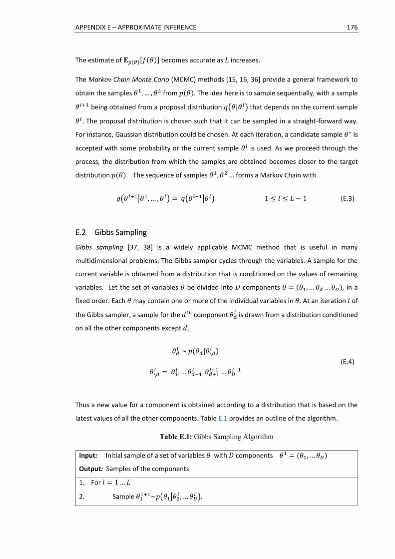
APPENDIX E – APPROXIMATE INFERENCE 176
The estimate of 𝔼𝑝(𝜃)[𝑓(휃)] becomes accurate as 𝐿 increases.
The Markov Chain Monte Carlo (MCMC) methods [15, 16, 36] provide a general framework to
obtain the samples 휃1, … , 휃𝐿 from 𝑝(휃). The idea here is to sample sequentially, with a sample
휃𝑙+1 being obtained from a proposal distribution 𝑞(휃|휃𝑙) that depends on the current sample
휃𝑙. The proposal distribution is chosen such that it can be sampled in a straight-forward way.
For instance, Gaussian distribution could be chosen. At each iteration, a candidate sample 휃∗ is
accepted with some probability or the current sample 휃𝑙 is used. As we proceed through the
process, the distribution from which the samples are obtained becomes closer to the target
distribution 𝑝(휃). The sequence of samples 휃1, 휃2 … forms a Markov Chain with
𝑞(휃𝑙+1|휃1, … , 휃𝑙) = 𝑞(휃𝑙+1|휃𝑙) 1 ≤ 𝑙 ≤ 𝐿 − 1 (E.3)
E.2 Gibbs Sampling
Gibbs sampling [37, 38] is a widely applicable MCMC method that is useful in many
multidimensional problems. The Gibbs sampler cycles through the variables. A sample for the
current variable is obtained from a distribution that is conditioned on the values of remaining
variables. Let the set of variables 휃 be divided into 𝐷 components 휃 = (휃1, … 휃𝑑 … 휃𝐷), in a
fixed order. Each 휃 may contain one or more of the individual variables in 휃. At an iteration 𝑙 of
the Gibbs sampler, a sample for the 𝑑𝑡ℎ component 휃𝑑𝑙 is drawn from a distribution conditioned
on all the other components except 𝑑.
휃𝑑𝑙 ~ 𝑝(휃𝑑|휃\𝑑
𝑙 )
휃\𝑑𝑙 = 휃1
𝑙 , … 휃𝑑−1𝑙 , 휃𝑑+1
𝑙−1 … 휃𝐷𝑙−1
(E.4)
Thus a new value for a component is obtained according to a distribution that is based on the
latest values of all the other components. Table E.1 provides an outline of the algorithm.
Table E.1: Gibbs Sampling Algorithm
Input: Initial sample of a set of variables 휃 with 𝐷 components 휃1 = (휃1, … 휃𝐷)
Output: Samples of the components
1. For 𝑙 = 1 … 𝐿
2. Sample 휃11+1~𝑝(휃1|휃2
𝑙 , … 휃𝐷𝑙 ).

APPENDIX E – APPROXIMATE INFERENCE 177
Gibbs sampling is particularly efficient if conditionally conjugate priors can be used. Consider for
example two Gaussian random variables X0 and X1 that are mixed to give a random variable X
in the following manner:
X0 ~ 𝒩(𝜇0, Σ0) X1 ~ 𝒩(𝜇1, Σ1)
(E.5)
𝑋 = 𝑍 X0 + (1 − 𝑍)X1
Here 𝑍 is a Bernoulli random variable that takes the value 1 with probability 𝜚. It indicates the
Gaussian from which 𝑋 is drawn. The joint density function is written as
𝑝(𝑥1 … 𝑥𝑁 , 𝑧1 … 𝑧𝑁, 𝜚, 𝜇0, Σ0, 𝜇1, Σ1) = (∏ 𝑝(𝑥𝑛|𝑧𝑛, 𝜇𝑧𝑛 , Σ𝑧𝑛)𝑝(𝑧𝑛|𝜚)
𝑁
𝑛=1
) ×
𝑝0(𝜚) 𝑝0(𝜇0, Σ0) 𝑝0(𝜇1, Σ1)
(E.6)
where 𝑥𝑛 is an observed value, 𝑧𝑛 is the Gaussian from which 𝑥𝑛 was drawn and 𝑝0 denotes a
prior distribution. The set of variables is 휃 = (𝜇0, Σ0, 𝜇1, Σ1, 𝜚, 𝑧1 … 𝑧𝑁). When sampling the
posterior 𝑝(휃|𝑥1. . 𝑥𝑁), Gibbs sampling is applied. The variables are sampled one at a time, with
the assumption that the values of the other variables are available. A conjugate prior can then
be assigned to the variable being sampled and the posterior for a variable can be computed
analytically. The Gibbs sampler for the above two mixture Gaussian cycles through as follows:
(i) Sample 𝜇0|Σ0, 𝑧1 … 𝑧𝑁, 𝑥1 … 𝑥𝑁. By assigning the mean parameter a Gaussian prior,
the posterior values can be sampled from an updated Gaussian distribution as per
equation (C.15).
(ii) Sample Σ0|𝜇0, 𝑧1 … 𝑧𝑁, 𝑥1 … 𝑥𝑁. By assigning the covariance parameter an Inverse-
Wishart prior, the posterior values can be sampled from an updated Inverse-Wishart
distribution as per equation (C.17).
(iii) Sample 𝜇1 and Σ1 in a similar way to (i) and (ii) respectively.
(iv) Sample 𝜚|𝑧1 … 𝑧𝑁. By assigning 𝜚 a Beta prior, the posterior values can be sampled
as per equation (C.12).
(v) Sample 𝑧1 … 𝑧𝑁|𝜚 by sampling from the Bernoulli distribution.
3. Sample 휃21+1~𝑝(휃2|휃1
𝑙+1, 휃3𝑙 , … 휃𝐷
𝑙 ).
4. …
5. Sample 휃𝐷1+1~𝑝(휃𝐷|휃1
𝑙+1, … 휃𝑑−1𝑙+1 ).
6. End For

APPENDIX E – APPROXIMATE INFERENCE 178
The Gibbs sampler relies on defining a conditional distribution 𝑝(휃𝑘|휃\𝑘) from which it is easy
to draw samples. In the above case sampling is easy because conjugate priors are used. Since
Gibbs sampling allows the variables to be partitioned, it is ideally suited for inference in graphical
models.
E.3 Slice Sampling
It is not always possible to have a conjugate prior for a variable, as observed in the subsequent
chapters. One option is to choose an appropriate proposal distribution that will lead to efficient
sampling. An alternative option is to treat a multivariate variable as univariate and apply Gibbs
sampling to draw samples for each dimension of the variable given the value of other
dimensions. Both these options need special coding and sometimes complex parameter tuning.
Slice sampling [39] provides a way of sampling from a density function which is known up to a
scale factor. It uses the principle that one can sample from a univariate distribution by sampling
uniformly from the region under the density curve. Let 휃 be the variable of interest and let 𝑓(휃)
be a function that is proportional to the density of 휃. The slice sampling technique involves
augmenting 휃 with an additional auxiliary variable 𝑢 and then drawing samples from the joint
(휃, 𝑢) space and ignoring the 𝑢 values. The algorithm has the following steps:
(i) Given a sample 휃𝑡, evaluate 𝑓(휃𝑡) and sample 𝑢 uniformly in the range
0 ≤ 𝑢 ≤ 𝑓(휃𝑡). The auxiliary variable 𝑢 represents a horizontal “slice” of the
distribution.
(ii) Define a region 휃𝑚𝑖𝑛 ≤ 휃𝑡 ≤ 휃𝑚𝑎𝑥 around the sample 휃𝑡 that encompasses as
much of the slice as possible.
(iii) Draw a new sample 휃𝑡+1~ { 휃′ ∈ 휃𝑚𝑖𝑛 ≤ 휃𝑡 ≤ 휃𝑚𝑎𝑥 ∶ 𝑢 < 𝑓(휃′)}.
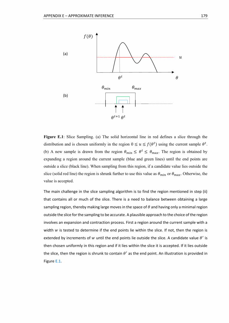
APPENDIX E – APPROXIMATE INFERENCE 179
Figure E.1: Slice Sampling. (a) The solid horizontal line in red defines a slice through the
distribution and is chosen uniformly in the region 0 ≤ 𝑢 ≤ 𝑓(휃𝑡) using the current sample 휃𝑡.
(b) A new sample is drawn from the region 휃𝑚𝑖𝑛 ≤ 휃𝑡 ≤ 휃𝑚𝑎𝑥. The region is obtained by
expanding a region around the current sample (blue and green lines) until the end points are
outside a slice (black line). When sampling from this region, if a candidate value lies outside the
slice (solid red line) the region is shrunk further to use this value as 휃𝑚𝑖𝑛 or 휃𝑚𝑎𝑥. Otherwise, the
value is accepted.
The main challenge in the slice sampling algorithm is to find the region mentioned in step (ii)
that contains all or much of the slice. There is a need to balance between obtaining a large
sampling region, thereby making large moves in the space of 휃 and having only a minimal region
outside the slice for the sampling to be accurate. A plausible approach to the choice of the region
involves an expansion and contraction process. First a region around the current sample with a
width 𝑤 is tested to determine if the end points lie within the slice. If not, then the region is
extended by increments of 𝑤 until the end points lie outside the slice. A candidate value 휃′ is
then chosen uniformly in this region and if it lies within the slice it is accepted. If it lies outside
the slice, then the region is shrunk to contain 휃′ as the end point. An illustration is provided in
Figure E.1.
휃𝑡
𝑢
𝑓(휃)
휃
휃𝑡 휃𝑡+1
휃𝑚𝑖𝑛 휃𝑚𝑎𝑥
(a)
(b)

180
References
[1] Dimitrova, N., Zhang, H. J., Shahraray, B., Sezan, I., Huang, T., & Zakhor, A. "Applications of
video-content analysis and retrieval." IEEE Multimedia 9, no. 3, (2002): 42-55.
[2] O'Hara, K., Gonzalez, G., Sellen, A., Penney, G., Varnavas, A., Mentis, H., & Carrell, T et al.
"Touchless interaction in surgery." Communications of the ACM 57, no. 1 (2014): 70-77.
[3] Atmosukarto, I., Ghanem, B., Ahuja, S., Muthuswamy, K., & Ahuja, N. "Automatic recognition
of offensive team formation in american football plays." Computer Vision and Pattern
Recognition Workshops (2013), pp. 991-998.
[4] Aggarwal, J. K., & Ryoo, M. S. "Human activity analysis: A review." ACM Computing Surveys
(CSUR) 43, no. 3 (2011): 16.
[5] Aggarwal, J. K., & Xia, L. "Human activity recognition from 3d data: A review." Pattern
Recognition Letters 48 (2014): 70-80.
[6] Chen, L., Wei, H., & Ferryman, J. "A survey of human motion analysis using depth imagery."
Pattern Recognition Letters 34, no. 15 (2013): 1995-2006.
[7] Plagemann, C., Ganapathi, V., Koller, D., & Thrun, S. "Real-time identification and localization
of body parts from depth images." Robotics and Automation (ICRA), (2010), pp. 3108-3113.
[8] Marr, D., Poggio, T., Hildreth, E. C., & Grimson, W. E. L. "A computational theory of human
stereo vision." Proceedings of the Royal Society of London B: Biological Sciences 204, no.
1156 (1979): 301-328.
[9] Shotton, J., Girshick, R., Fitzgibbon, A., Sharp, T., Cook, M., Finocchio, M., & Blake, A et al.
"Efficient human pose estimation from single depth images." Pattern Analysis and Machine
Intelligence 35, no. 12 (2013): 2821-2840.
[10] Zhang, Z. "Microsoft Kinect sensor and its effect." IEEE MultiMedia 19, no. 2, (2012): 4-10.
[11] Xia, L., Chen, C. C., & Aggarwal, J. K, 2012, June. "View invariant human action recognition
using histograms of 3d joints." Computer Vision and Pattern Recognition Workshops, (2012),
pp. 20-27.

REFERENCES 181
[12] Johansson, G. "Visual perception of biological motion and a model for its analysis." Attention,
Perception, & Psychophysics 14, no. 2 (1973): 201-211.
[13] Puce, A., & Perrett, D. "Electrophysiology and brain imaging of biological motion."
Philosophical Transactions of the Royal Society of London B: Biological Sciences 358, no. 1431
(2003): 435-445.
[14] Shotton, J., Sharp, T., Kipman, A., Fitzgibbon, A., Finocchio, M., Blake, A., & Moore, R et al.
“Real-time human pose recognition in parts from single depth images”. Communications of
the ACM 56, no. 1 (2013): 116-124.
[15] Koller, D., & Friedman, N. Probabilistic Graphical Models: Principles and Techniques. MIT
press, 2009.
[16] Bishop, C. M. Pattern Recognition and Machine Learning. Springer, 2006.
[17] Ghahramani, Z. "An introduction to hidden Markov models and Bayesian networks."
International Journal of Pattern Recognition and Artificial Intelligence 15, no. 01 (2001): 9-
42.
[18] Orbanz, P., & Teh, Y. W. "Bayesian nonparametric models." Encyclopedia of Machine
Learning, (2010), pp. 81-89, Springer US.
[19] Teh, Y. W. "Dirichlet process." Encyclopedia of Machine Learning, (2010), pp. 280-287.
[20] Khoshelham, K. "Accuracy analysis of Kinect depth data." ISPRS workshop laser scanning,
(2011), vol. 38, no. 5, p. W12.
[21] Sansoni, G., Trebeschi, M., & Docchio, F. "State-of-the-art and applications of 3D imaging
sensors in industry, cultural heritage, medicine, and criminal investigation." Sensors 9, no. 1
(2009): 568-601.
[22] Sarbolandi, H., Lefloch, D., & Kolb, A. "Kinect range sensing: Structured-light versus time-of-
flight Kinect." Computer Vision and Image Understanding, 139, (2015): 1-20.
[23] Trucco, E., & Verri, A. Introductory Techniques for 3-D Computer Vision. Vol. 201. Englewood
Cliffs: Prentice Hall, 1998.
[24] Hartley, R., & Zisserman, A. Multiple View Geometry in Computer Vision. Cambridge
University Press, 2003.
[25] Time-of-Flight and Kinect Imaging. Retrieved from
campar.in.tum.de/twiki/pub/Chair/TeachingSs11Kinect/2011-
DSensors_LabCourse_Kinect.pdf

REFERENCES 182
[26] The Science Behind Kinects or Kinect 1.0 versus 2.0. Retrieved from
gamasutra.com/blogs/DanielLau/20131127/205820/The_Science_Behind_Kinects_or_Kine
ct_10_versus_20.php
[27] Felzenszwalb, P. F., & Huttenlocher, D. P. "Pictorial structures for object recognition."
International Journal of Computer Vision 61, no. 1 (2005): 55-79.
[28] Kohli, P., & Shotton, J. "Key developments in human pose estimation for Kinect." Consumer
Depth Cameras for Computer Vision, (2013), pp. 63-70.
[29] Jordan, M. I. "Graphical models." Statistical Science (2004): 140-155.
[30] Barber, D. Bayesian Reasoning and Machine Learning. Cambridge University Press, 2012.
[31] Jordan, M. I., & Weiss, Y. "Probabilistic inference in graphical models." Handbook of Neural
Networks and Brain Theory (2002).
[32] Rabiner, L. R., & Juang, B. H. "An introduction to hidden Markov models." IEEE ASSP
Magazine, 3, no. 1 (1986): 4-16.
[33] Sutton, C., & McCallum, A. "An introduction to conditional random fields." Machine Learning
4, no. 4 (2011): 267-373.
[34] Glickman, M. E., & van Dyk, D. A. "Basic Bayesian methods." Topics in Biostatistics (2007):
319-338.
[35] Duda, R. O., Hart, P. E., & Stork, D. G. Pattern Classification. John Wiley & Sons, 2012.
[36] Gelman, A., Carlin, J. B., Stern, H. S., & Rubin, D. B. Bayesian Data Analysis. Chapman & Hall,
2014.
[37] Resnik, P., & Hardisty, E. “Gibbs sampling for the uninitiated”. No. CS-TR-4956. Maryland Univ
College Park Inst. for Advanced Computer Studies, 2010.
[38] Geman, S., & Geman, D. "Stochastic relaxation, Gibbs distributions, and the Bayesian
restoration of images." Pattern Analysis and Machine Intelligence 6, (1984): 721-741.
[39] Neal, R. M. "Slice sampling." Annals of Statistics (2003): 705-741.
[40] Sudderth, E. B. "Graphical models for visual object recognition and tracking." PhD diss.,
Massachusetts Institute of Technology, 2006.
[41] Fox, E. B. "Bayesian nonparametric learning of complex dynamical phenomena." PhD diss.,
Massachusetts Institute of Technology, 2009.
[42] Antoniak, C. E. "Mixtures of Dirichlet processes with applications to Bayesian nonparametric
problems." The Annals of Statistics (1974): 1152-1174.

REFERENCES 183
[43] Sethuraman, J. "A constructive definition of Dirichlet priors." Statistica Sinica (1994): 639-
650.
[44] Teh, Y. W., Jordan, M. I., Beal, M. J., & Blei, D. M. "Hierarchical Dirichlet processes." Journal
of the American Statistical Association (2012).
[45] Hjort, N. L., Holmes, C., Müller, P., & Walker, S. G, eds. Bayesian Nonparametrics. Vol. 28.
Cambridge University Press, 2010.
[46] Orbanz, P. "Lecture notes on Bayesian nonparametrics." Journal of Mathematical Psychology
56 (2012): 1-12.
[47] Li, S. Z. Markov Random Field Modeling in Image Analysis. Springer Science & Business Media,
2009.
[48] Birney, E. "Hidden Markov models in biological sequence analysis." IBM Journal of Research
and Development 45, no. 3.4 (2001): 449-454.
[49] Chou, W., & Li, L. "A minimum classification error (MCE) framework for generalized linear
classifier in machine learning for text categorization/retrieval." Machine Learning and
Applications, (2004), pp. 26-33.
[50] Genon-Catalot, V., Jeantheau, T., & Larédo, C. "Stochastic volatility models as hidden Markov
models and statistical applications." Bernoulli 6, no. 6 (2000): 1051-1079.
[51] Jelinek, F. Statistical Methods for Speech Recognition. MIT press, 1997.
[52] DeCaprio, D., Vinson, J. P., Pearson, M. D., Montgomery, P., Doherty, M., & Galagan, J. E.
"Conrad: gene prediction using conditional random fields." Genome research 17, no. 9
(2007): 1389-1398.
[53] Koppula, H., & Saxena, A. "Learning spatio-temporal structure from rgb-d videos for human
activity detection and anticipation." International Conference on Machine Learning (2013),
pp. 792-800.
[54] Shen, D., Sun, J. T., Li, H., Yang, Q., & Chen, Z. "Document summarization using conditional
random fields." International Joint Conference on Artifical Intelligence, (2007), vol. 7, pp.
2862-2867.
[55] Poppe, R. "Vision-based human motion analysis: An overview." Computer Vision and Image
Understanding 108, no. 1 (2007): 4-18.
[56] VidCon 2015 Haul: Trends, Strategic Insights, Critical Data, and Tactical Advice. Retrieved
from reelseo.com/vidcon-2015-strategic-insights-tactical-advice/

REFERENCES 184
[57] How many cameras in the UK?. Retrieved from securitynewsdesk.com/how-many-cctv-
cameras-in-the-uk/
[58] Forsyth, D. A., Arikan, O., & Ikemoto, L. Computational Studies of Human Motion: Tracking
and Motion Synthesis. Now Publishers Inc, 2006.
[59] Russakovsky, O., Deng, J., Su, H., Krause, J., Satheesh, S., Ma, S., & Berg, A. C et al. "Imagenet
large scale visual recognition challenge." International Journal of Computer Vision 115, no. 3
(2015): 211-252.
[60] DARPA Mind’s eye program : Broad agency announcement. Retrieved from fbo.gov/
[61] Biliński, P. T. "Human action recognition in videos." PhD diss., Université Nice Sophia
Antipolis, 2014.
[62] Kinect for Xbox One. Retrieved from xbox.com/en-US/xbox-one/accessories/kinect-for-xbox-
one
[63] Kasteren, T. L. M. "Activity recognition for health monitoring elderly using temporal
probabilistic models." PhD diss., Informatics Institute, 2011.
[64] Lasserre, J. A., Bishop, C. M., & Minka, T. P. "Principled hybrids of generative and
discriminative models." Computer Vision and Pattern Recognition, (2006), vol. 1, pp. 87-94.
[65] Steinwart, I, and Christmann, A. Support Vector Machines. Springer Science & Business
Media, 2008.
[66] Paisley, J., Wang, C., & Blei, D. M. "The discrete infinite logistic normal distribution." Bayesian
Analysis 7, no. 4 (2012): 997-1034.
[67] Murray, I., Adams, R. P., & MacKay, D. J. "Elliptical slice sampling." arXiv preprint
arXiv:1001.0175 (2009).
[68] Sudderth, E. B., Torralba, A., Freeman, W. T., & Willsky, A. S. "Describing visual scenes using
transformed objects and parts." International Journal of Computer Vision 77, no. 1-3 (2008):
291-330.
[69] Van Gael, J., Saatci, Y., Teh, Y. W., & Ghahramani, Z. "Beam sampling for the infinite Hidden
Markov Model." International conference on Machine learning, (2008), pp. 1088-1095.
[70] Kalli, M., Griffin, J. E., & Walker, S. G. "Slice sampling mixture models." Statistics and
Computing 21, no. 1 (2011): 93-105.
[71] Ishwaran, H., & Zarepour, M. "Markov chain Monte Carlo in approximate Dirichlet and beta
two-parameter process hierarchical models." Biometrika 87, no. 2 (2000): 371-390.

REFERENCES 185
[72] Cha, S. H. "Comprehensive survey on distance/similarity measures between probability
density functions." International Journal of Mathematical Models and Methods in Applied
Sciences, 4(1), (2007):300–3007.
[73] Gershman, S. J., & Blei, D. M. "A tutorial on Bayesian nonparametric models." Journal of
Mathematical Psychology 56, no. 1 (2012): 1-12.
[74] Li, W., Zhang, Z., & Liu, Z. "Action recognition based on a bag of 3d points." Computer Vision
and Pattern Recognition Workshops, (2010), pp. 9-14.
[75] Microsoft Developer Network, “Joint orientation, Kinect for Windows” Retrieved from
msdn.microsoft.com/en-us/library/hh973073.aspx
[76] Fox, E. B., Sudderth, E. B., Jordan, M. I., & Willsky, A. S. "A sticky HDP-HMM with application
to speaker diarization." The Annals of Applied Statistics (2011): 1020-1056.
[77] Dalal, N. and Triggs, B., 2005, June. "Histograms of oriented gradients for human detection."
Computer Vision and Pattern Recognition, (2005), vol. 1, pp. 886-893.
[78] Zhu, Y., Chen, W., & Guo, G.. "Evaluating spatiotemporal interest point features for depth-
based action recognition." Image and Vision Computing 32, no. 8 (2014): 453-464.
[79] Devanne, M., Wannous, H., Berretti, S., Pala, P., Daoudi, M., & Del Bimbo, A. "3-D human
action recognition by shape analysis of motion trajectories on Riemannian manifold." IEEE
Transactions on Cybernetics 45, no. 7 (2015): 1340-1352.
[80] Ohn-Bar, E., & Trivedi, M. "Joint angles similarities and HOG2 for action recognition."
Computer Vision and Pattern Recognition Workshops, (2013), pp. 465-470.
[81] Fine, S., Singer, Y., & Tishby, N. "The hierarchical hidden Markov model: Analysis and
applications." Machine Learning 32, no. 1 (1998): 41-62.
[82] Krishnapuram, B., Carin, L., Figueiredo, M. A., & Hartemink, A. J. "Sparse multinomial logistic
regression: Fast algorithms and generalization bounds." Pattern Analysis and Machine
Intelligence 27, no. 6 (2005): 957-968.
[83] Murphy, K. P., & Paskin, M. A. "Linear-time inference in hierarchical HMMs." Advances in
Neural Information Processing Systems 2 (2002): 833-840.
[84] Heller, K. A., Teh, Y. W., & Görür, D. "Infinite hierarchical hidden Markov models."
International Conference on Artificial Intelligence and Statistics, (2009), pp. 224-231.
[85] Sung, J., Ponce, C., Selman, B., & Saxena, A. "Human activity detection from RGBD images."
Pattern, Activity, and Intent Recognition 64 (2011).

REFERENCES 186
[86] Müller, M., Röder, T., Clausen, M., Eberhardt, B., Krüger, B., & Weber, A. "Documentation
mocap database HDM05.", Technical report, No. CG-2007-2, ISSN 1610-8892, Universität
Bonn (2007).
[87] Song, S., & Xiao, J. "Tracking revisited using rgbd camera: Unified benchmark and baselines."
International Conference on Computer Vision, (2013), pp. 233-240.
[88] Wang, J., Liu, Z., Wu, Y., & Yuan, J. "Learning actionlet ensemble for 3D human action
recognition." Pattern Analysis and Machine Intelligence 36, no. 5 (2014): 914-927.
[89] Hu, J. F., Zheng, W. S., Lai, J., & Zhang, J. "Jointly learning heterogeneous features for RGB-D
activity recognition." Computer Vision and Pattern Recognition, (2015), pp. 5344-5352.
[90] Shan, J., & Akella, S.. "3D human action segmentation and recognition using pose kinetic
energy." Advanced Robotics and its Social Impacts (ARSO), (2014), pp. 69-75.
[91] Kurihara, K., Welling, M., & Teh, Y. W. "Collapsed variational Dirichlet process mixture
models." International Joint Conferences on Artificial Intelligence, vol. 7, (2007), pp. 2796-
2801.
[92] Johnson, M. J., and Willsky, A. S. "Bayesian nonparametric hidden semi-Markov models." The
Journal of Machine Learning Research 14, no. 1 (2013): 673-701.
[93] Figueiredo, M. A. "Adaptive sparseness for supervised learning." Pattern Analysis and
Machine Intelligence 25, no. 9 (2003): 1150-1159.
[94] Jordan, A. "On discriminative vs. generative classifiers: A comparison of logistic regression
and naive bayes." Advances in Neural Information Processing Systems 14 (2002): 841.
[95] Quattoni, A., Wang, S., Morency, L. P., Collins, M., & Darrell, T. "Hidden conditional random
fields." IEEE Transactions on Pattern Analysis & Machine Intelligence 10 (2007): 1848-1852.
[96] Gunawardana, A., Mahajan, M., Acero, A., & Platt, J. C. "Hidden conditional random fields for
phone classification." INTERSPEECH (2005), pp. 1117-1120.
[97] Qi, Y., Szummer, M., & Minka, T. P. "Bayesian conditional random fields." International
Workshop on Artificial Intelligence and Statistics, (2005), pp. 269-276.
[98] Bhattacharya, A., Pati, D., Pillai, N. S., & Dunson, D. B. "Dirichlet–Laplace priors for optimal
shrinkage." Journal of the American Statistical Association 110, no. 512 (2015): 1479-1490.
[99] Kotz, S., Kozubowski, T., & Podgorski, K. The Laplace Distribution and Generalizations: A
Revisit with Applications to Communications, Economics, Engineering, and Finance. Springer
Science & Business Media, 2012.

REFERENCES 187
[100] Eltoft, T., Kim, T., & Lee, T. W. "On the multivariate Laplace distribution." Signal Processing
Letters 13, no. 5 (2006): 300-303.
[101] Park, T., & Casella, G. "The Bayesian lasso." Journal of the American Statistical Association
103, no. 482 (2008): 681-686.
[102] Gaglio, S., Re, G. L., & Morana, M. "Human activity recognition process using 3-D posture
data." IEEE Transactions on Human-Machine Systems 45, no. 5 (2015): 586-597.
[103] Dittmar, D. "Slice Sampling." TU Darmstadt. Retrieved from ausy. informatik. tu-darmstadt.
de/uploads/Teaching/RobotLearningSeminar/Dittmar_RLS_2013. pdf (2013).
[104] Yamato, J., Ohya, J., & Ishii, K. "Recognizing human action in time-sequential images using
hidden Markov model." Computer Vision and Pattern Recognition, (1992), pp. 379-385.
[105] Aggarwal, J. K., and Cai, Q. "Human motion analysis: A review." Nonrigid and Articulated
Motion Workshop, (1997), pp. 90-102.
[106] Moeslund, T. B., Hilton, A., & Krüger, V.. "A survey of advances in vision-based human motion
capture and analysis." Computer Vision and Image Understanding 104, no. 2 (2006): 90-126.
[107] Turaga, P., Chellappa, R., Subrahmanian, V. S., & Udrea, O. "Machine recognition of human
activities: A survey." Circuits and Systems for Video Technology, IEEE Transactions on 18, no.
11 (2008): 1473-1488.
[108] Weinland, D., Ronfard, R., & Boyer, E. "A survey of vision-based methods for action
representation, segmentation and recognition." Computer Vision and Image Understanding
115, no. 2 (2011): 224-241.
[109] Chaquet, J. M., Carmona, E. J., & Fernández-Caballero, A. " A survey of video datasets for
human action and activity recognition." Computer Vision and Image Understanding 117, no.
6 (2013): 633-659.
[110] Cheng, G., Wan, Y., Saudagar, A. N., Namuduri, K., & Buckles, B. P. "Advances in human action
recognition: A survey." arXiv preprint arXiv:1501.05964 (2015).
[111] Han, J., Shao, L., Xu, D., & Shotton, J. "Enhanced computer vision with Microsoft Kinect
sensor: A review." IEEE Transactions on Cybernetics 43, no. 5 (2013): 1318-1334.
[112] Ye, M., Zhang, Q., Wang, L., Zhu, J., Yang, R., & Gall, J. "A survey on human motion analysis
from depth data." Time-of-Flight and Depth Imaging. Sensors, Algorithms, and Applications,
(2013), pp. 149-187.
[113] Chen, C., Jafari, R., & Kehtarnavaz, N. "A survey of depth and inertial sensor fusion for human
action recognition." Multimedia Tools and Applications (2015): 1-21.

REFERENCES 188
[114] Presti, L. L., & La Cascia, M. "3D skeleton-based human action classification: A survey."
Pattern Recognition 53, no. C (2016): 130-147.
[115] Davis, J. W., & Bobick, A. E.. "The representation and recognition of human movement using
temporal templates." Computer Vision and Pattern Recognition, (1997), pp. 928-934.
[116] Wang, Y., Huang, K., & Tan, T. "Human activity recognition based on r transform." Computer
Vision and Pattern Recognition, (2007), pp. 1-8.
[117] Blank, M., Gorelick, L., Shechtman, E., Irani, M., & Basri, R. "Actions as space-time shapes."
International Conference on Computer Vision, (2005), vol. 2, pp. 1395-1402.
[118] Yu, E., & Aggarwal, J. K. "Human action recognition with extremities as semantic posture
representation." Computer Vision and Pattern Recognition Workshops, (2009), pp. 1-8.
[119] Qian, H., Mao, Y., Xiang, W., & Wang, Z. "Recognition of human activities using SVM multi-
class classifier." Pattern Recognition Letters 31, no. 2 (2010): 100-111.
[120] Ni, B., Wang, G., & Moulin, P. "Rgbd-hudaact: A color-depth video database for human daily
activity recognition." Consumer Depth Cameras for Computer Vision, (2013), pp. 193-208.
[121] Jalal, A., Uddin, M. Z., Kim, J. T., & Kim, T. S. "Recognition of human home activities via depth
silhouettes and ℜ transformation for smart homes." Indoor and Built Environment (2011):
1420326X11423163.
[122] Yang, X., Zhang, C., & Tian, Y. "Recognizing actions using depth motion maps-based
histograms of oriented gradients." International Conference on Multimedia, (2012), pp.
1057-1060.
[123] Vieira, A. W., Nascimento, E. R., Oliveira, G. L., Liu, Z., & Campos, M. F. "Stop: Space-time
occupancy patterns for 3d action recognition from depth map sequences." Progress in
Pattern Recognition, Image Analysis, Computer Vision, and Applications, (2012), pp. 252-259.
[124] Oreifej, O., & Liu, Z. "Hon4d: Histogram of oriented 4d normals for activity recognition from
depth sequences." Computer Vision and Pattern Recognition, pp. 716-723. 2013.
[125] Efros, A. A., Berg, A. C., Mori, G., & Malik, J. "Recognizing action at a distance." International
Conference on Computer Vision, (2003), pp. 726-733.
[126] Ikizler-Cinbis, N., & Sclaroff, S. "Object, scene and actions: Combining multiple features for
human action recognition." European Conference on Computer Vision (2010): 494-507.
[127] Ballin, G., Munaro, M., & Menegatti, E. "Human action recognition from rgb-d frames based
on real-time 3d optical flow estimation." Biologically Inspired Cognitive Architectures, (2013),
pp. 65-74.

REFERENCES 189
[128] Laptev, I. "On space-time interest points." International Journal of Computer Vision 64, no.
2-3 (2005): 107-123.
[129] Oikonomopoulos, A., Patras, I., & Pantic, M. "Spatiotemporal salient points for visual
recognition of human actions." IEEE Transactions on Systems, Man, and Cybernetics 36, no.
3 (2005): 710-719.
[130] Rapantzikos, K., Avrithis, Y., & Kollias, S. "Spatiotemporal saliency for event detection and
representation in the 3D wavelet domain: potential in human action recognition."
International Conference on Image and Video Retrieval, (2007), pp. 294-301.
[131] Klaser, A., Marszałek, M., & Schmid, C. "A spatio-temporal descriptor based on 3d-gradients."
British Machine Vision Conference, (2008), pp. 275-1.
[132] Laptev, I., Marszałek, M., Schmid C., & Rozenfeld, B. "Learning realistic human actions from
movies." Computer Vision and Pattern Recognition, (2008), pp. 1-8.
[133] Emonet, R., Varadarajan, J., & Odobez, J. M. "Temporal analysis of motif mixtures using
Dirichlet processes." Pattern Analysis and Machine Intelligence, (2014), 36(1), 140-156.
[134] Zhu, Y., Chen, W., & Guo, G. "Evaluating spatiotemporal interest point features for depth-
based action recognition." Image and Vision Computing 32, no. 8 (2014): 453-464.
[135] Dollár, P., Rabaud, V., Cottrell, G., & Belongie, S. "Behavior recognition via sparse spatio-
temporal features." Visual Surveillance and Performance Evaluation of Tracking and
Surveillance, (2005), pp. 65-72.
[136] Zhang, H., & Parker, L. E. "4-dimensional local spatio-temporal features for human activity
recognition." Intelligent Robots and Systems, (2011), pp. 2044-2049.
[137] Xia, L. and Aggarwal, J.K. "Spatio-temporal depth cuboid similarity feature for activity
recognition using depth camera. " Computer Vision and Pattern Recognition, (2013), pp.
2834-2841.
[138] Rahmani, H., Mahmood, A., Huynh, D. Q., & Mian, A. "HOPC: Histogram of oriented principal
components of 3D pointclouds for action recognition." European Conference on Computer
Vision, (2014), pp. 742-757.
[139] Zhao, Y., Liu, Z., Yang, L., & Cheng, H. "Combing rgb and depth map features for human
activity recognition." Signal & Information Processing Association Annual Summit and
Conference, (2012), pp. 1-4.
REFERENCES 190
[140] Cheng, Z., Qin, L., Ye, Y., Huang, Q., & Tian, Q. "Human daily action analysis with multi-view
and color-depth data." European Conference on Computer Vision Workshops and
Demonstrations, (2012), pp. 52-61.
[141] Wang, J., Liu, Z., Chorowski, J., Chen, Z. and Wu, Y., "Robust 3d action recognition with
random occupancy patterns." European Conference on Computer Vision, (2012), pp. 872-
885.
[142] Sigal, L. "Human pose estimation." Computer Vision (2014), pp. 362-370.
[143] Kuettel, D., Breitenstein, M. D., Van Gool, L., & Ferrari, V. "What's going on? Discovering
spatio-temporal dependencies in dynamic scenes." Computer Vision and Pattern
Recognition, (2010), pp. 1951-1958.
[144] Poppe, R. "Vision-based human motion analysis: An overview." Computer Vision and Image
Understanding 108, no. 1 (2007): 4-18.
[145] Hospedales, T., Gong, S., & Xiang, T. "A Markov clustering topic model for mining behaviour
in video." International Conference on Computer Vision, (2009), pp. 1165-1172.
[146] Varadarajan, J., Emonet, R., & Odobez, J. M. "A sequential topic model for mining recurrent
activities from long term video logs." International Journal of Computer Vision, (2013),
103(1), 100-126.
[147] Yang, X., & Tian, Y. "Eigenjoints-based action recognition using naive-Bayes-nearest-
neighbor." Computer Vision and Pattern Recognition Workshops, (2012), pp. 14-19.
[148] Ellis, C., Masood, S. Z., Tappen, M. F., Laviola Jr, J. J., & Sukthankar, R. "Exploring the trade-
off between accuracy and observational latency in action recognition." International Journal
of Computer Vision 101, no. 3 (2013): 420-436.
[149] Raptis, M., Kirovski, D., & Hoppe, H. "Real-time classification of dance gestures from skeleton
animation." SIGGRAPH/Eurographics Symposium on Computer Animation, (2011), pp. 147-
156.
[150] Miranda, L., Vieira, T., Martínez, D., Lewiner, T., Vieira, A. W., & Campos, M. F. "Online
gesture recognition from pose kernel learning and decision forests." Pattern Recognition
Letters 39 (2014): 65-73.
[151] Lillo, I., Soto, A., & Niebles, J. "Discriminative hierarchical modeling of spatio-temporally
composable human activities." Computer Vision and Pattern Recognition, (2014), pp. 812-
819.

REFERENCES 191
[152] Zhang, C., & Tian, Y. "Rgb-d camera-based daily living activity recognition." Journal of
Computer Vision and Image Processing 2, no. 4 (2012): 12.
[153] Ofli, F., Chaudhry, R., Kurillo, G., Vidal, R., & Bajcsy, R. "Sequence of the most informative
joints (SMIJ): A new representation for human skeletal action recognition." Journal of Visual
Communication and Image Representation 25, no. 1 (2014): 24-38.
[154] Sempena, S., Maulidevi, N. U., & Aryan, P. R. "Human action recognition using dynamic time
warping." International Conference on Electrical Engineering and Informatics, (2011), pp. 1-
5.
[155] Vemulapalli, R., Arrate, F., & Chellappa, R. "R3DG features: Relative 3D geometry-based
skeletal representations for human action recognition." Computer Vision and Image
Understanding, (2016).
[156] Evangelidis, G., Singh, G., & Horaud, R. "Skeletal quads: Human action recognition using joint
quadruples." International Conference on Pattern Recognition, (2014), pp. 4513-4518.
[157] Gowayyed, M. A., Torki, M., Hussein, M. E., & El-Saban, M. "Histogram of oriented
displacements (HOD): Describing trajectories of human joints for action recognition."
International Joint Conference on Artificial Intelligence, (2013).
[158] Hussein, M. E., Torki, M., Gowayyed, M. A., & El-Saban, M. "Human action recognition using
a temporal hierarchy of covariance descriptors on 3D joint locations." International Joint
Conference on Artificial Intelligence, (2013), vol. 13, pp. 2466-2472.
[159] Yun, K., Honorio, J., Chattopadhyay, D., Berg, T. L., & Samaras, D. "Two-person interaction
detection using body-pose features and multiple instance learning." Computer Vision and
Pattern Recognition Workshops, (2012), pp. 28-35.
[160] Eweiwi, A., Cheema, M. S., Bauckhage, C., & Gall, J. "Efficient pose-based action recognition."
Asian Conference on Computer Vision, (2014), pp. 428-443.
[161] Climent-Pérez, P., Chaaraoui, A. A., Padilla-López, J. R., & Flórez-Revuelta, F. "Optimal joint
selection for skeletal data from RGB-D devices using a genetic algorithm." Advances in
Computational Intelligence, (2012), pp. 163-174.
[162] Anirudh, R., Turaga, P., Su, J., & Srivastava, A. "Elastic functional coding of human actions:
from vector-fields to latent variables." Proceedings of the IEEE Conference on Computer
Vision and Pattern Recognition, (2015), pp. 3147-3155.
[163] Slama, R., Wannous, H., Daoudi, M., & Srivastava, A. "Accurate 3D action recognition using
learning on the Grassmann manifold." Pattern Recognition 48, no. 2 (2015): 556-567.

REFERENCES 192
[164] Jiang, H. "Discriminative training of HMMs for automatic speech recognition: A survey."
Computer Speech & Language 24, no. 4 (2010): 589-608.
[165] He, X., Deng, L., & Chou, W. "Discriminative learning in sequential pattern recognition." Signal
Processing Magazine 25, no. 5 (2008): 14-36.
[166] Yu, D., and Deng, L. "Large-margin discriminative training of hidden Markov models for
speech recognition." International Conference on Semantic Computing, (2007), pp. 429-438.
[167] Nguyen, N. T., Phung, D. Q., Venkatesh, S., & Bui, H. "Learning and detecting activities from
movement trajectories using the hierarchical hidden Markov model." Computer Vision and
Pattern Recognition, (2005), vol. 2, pp. 955-960.
[168] Natarajan, P., and Nevatia, R. "Coupled hidden semi Markov models for activity recognition."
IEEE Workshop on Motion and Video Computing, (2007), pp. 10-10.
[169] Dai, P., Di, H., Dong, L., Tao, L., & Xu, G. "Group interaction analysis in dynamic context." IEEE
Transactions on Systems, Man, and Cybernetics, 38, no. 1 (2008): 275-282.
[170] Wang, S. B., Quattoni, A., Morency, L. P., Demirdjian, D., & Darrell, T., "Hidden conditional
random fields for gesture recognition." Computer Vision and Pattern Recognition, (2006),
vol. 2, pp. 1521-1527.
[171] Zhang, J., & Gong, S. "Action categorization with modified hidden conditional random field."
Pattern Recognition, (2010), 43(1), 197-203.
[172] Lin, T. H., Kaminski, N., & Bar-Joseph, Z. "Alignment and classification of time series gene
expression in clinical studies." Bioinformatics 24, no. 13 (2008): i147-i155.
[173] Müller, P., & Quintana, F. A. "Nonparametric Bayesian data analysis." Statistical Science
(2004): 95-110.
[174] Foti, N. J., & Williamson, S. A. "A survey of non-exchangeable priors for Bayesian
nonparametric models." Pattern Analysis and Machine Intelligence, 37, no. 2 (2015): 359-
371.
[175] Alexiou, I., Xiang, T., & Gong, S. "Learning a joint discriminative-generative model for action
recognition." International Conference on Systems, Signals and Image Processing, (2015), pp.
1-4.
[176] Huggins, J. H., & Wood, F. "Infinite structured hidden semi-Markov models." arXiv preprint
arXiv:1407.0044 (2014).
[177] Hughes, M. C., Kim, D. I., & Sudderth, E. B. "Reliable and scalable variational inference for the
hierarchical dirichlet process." Artificial Intelligence and Statistics Conference, (2015).

REFERENCES 193
[178] Hu, D. H., Zhang, X. X., Yin, J., Zheng, V. W., & Yang, Q. "Abnormal activity recognition based
on HDP-HMM models." International Joint Conference on Artificial Intelligence, (2009), pp.
1715-1720.
[179] Bargi, A., Xu, D., Yi, R., & Piccardi, M. "An adaptive online HDP-HMM for segmentation and
classification of sequential data." arXiv preprint arXiv:1503.02761 (2015).
[180] Kooij, J. F., Englebienne, G., & Gavrila, D. M. "A non-parametric hierarchical model to discover
behavior dynamics from tracks." European Conference on Computer Vision, (2012), pp. 270-
283.
[181] Gael, J. V., Teh, Y. W., & Ghahramani, Z. "The infinite factorial hidden Markov model."
Advances in Neural Information Processing Systems, (2009), pp. 1697-1704.
[182] Valera, I., Ruiz, F. J., & Perez-Cruz, F. "Infinite factorial unbounded hidden Markov model for
blind multiuser channel estimation." International Workshop on Cognitive Information
Processing, (2014), pp. 1-6.
[183] Mcauliffe, J. D., & Blei, D. M. "Supervised topic models." Advances in Neural Information
Processing Systems, (2008), pp. 121-128.
[184] Dai, A. M., & Storkey, A. J. "The supervised hierarchical Dirichlet process." Pattern Analysis
and Machine Intelligence 37, no. 2 (2015): 243-255.
[185] Bousmalis, K., Zafeiriou, S., Morency, L. P., & Pantic, M. "Infinite hidden conditional random
fields for human behavior analysis." Neural Networks and Learning Systems 24, no. 1 (2013):
170-177.
[186] Bousmalis, K., Zafeiriou, S., Morency, L.P., Pantic, M. and Ghahramani, Z., "Variational hidden
conditional random fields with coupled Dirichlet process mixtures. " Machine Learning and
Knowledge Discovery in Databases, (2013), pp. 531-547.
[187] Lin, L., Wang, K., Zuo, W., Wang, M., Luo, J., & Zhang, L. "A deep structured model with
radius–margin bound for 3D human activity recognition." International Journal of Computer
Vision (2015): 1-18.
[188] Shou, Z., Wang, D., & Chang, S. F. "Action Temporal Localization in Untrimmed Videos via
Multi-stage CNNs." arXiv preprint arXiv:1601.02129 (2016).
[189] Ryoo, M. S., & Matthies, L. "First-person activity recognition: feature, temporal structure, and
prediction." International Journal of Computer Vision (2015): 1-22.
[190] Sugiura, T., Goto, N., & Hayashi, A. "A discriminative model corresponding to hierarchical
HMMs." Intelligent Data Engineering and Automated Learning, (2007), pp. 375-384.
REFERENCES 194
[191] Shao, L., Han, J., Kohli, P., & Zhang, Z., (Eds.) Computer Vision and Machine Learning with
RGB-D Sensors. Springer, 2014.
[192] Raman, N., Maybank, S. J., & Zhang, D. "Action classification using a discriminative non-
parametric Hidden Markov Model." International Conference on Machine Vision, (2013), vol.
9067, pp. 10.
[193] Raman, N. & Maybank, S. J. "Action classification using a discriminative multilevel HDP-
HMM." Neurocomputing 154 (2015): 149-161.
[194] Raman, N. & Maybank, S. J. "Activity recognition using a supervised non-parametric
hierarchical HMM." Neurocomputing 199 (2016): 163-177.
[195] Raman, N. & Maybank, S. J. "Non-parametric hidden conditional random fields for action
classification." IEEE International Joint Conference on Neural Networks, preprint, (2016).