acquiring word-meaning mappings for natural language interfaces · 2006-01-11 · acquiring...

Journal of Artificial Intelligence Research 18 (2003) 1-44 Submitted 5/02; published 1/03

Acquiring Word-Meaning Mappingsfor Natural Language Interfaces

Cynthia A. Thompson [email protected]

School of Computing, University of UtahSalt Lake City, UT 84112-3320

Raymond J. Mooney [email protected]

Department of Computer Sciences, University of TexasAustin, TX 78712-1188

Abstract

This paper focuses on a system, Wolfie (WOrd Learning From Interpreted Exam-ples), that acquires a semantic lexicon from a corpus of sentences paired with semanticrepresentations. The lexicon learned consists of phrases paired with meaning represen-tations. Wolfie is part of an integrated system that learns to transform sentences intorepresentations such as logical database queries.

Experimental results are presented demonstrating Wolfie’s ability to learn usefullexicons for a database interface in four different natural languages. The usefulness ofthe lexicons learned by Wolfie are compared to those acquired by a similar system, withresults favorable to Wolfie. A second set of experiments demonstrates Wolfie’s abilityto scale to larger and more difficult, albeit artificially generated, corpora.

In natural language acquisition, it is difficult to gather the annotated data neededfor supervised learning; however, unannotated data is fairly plentiful. Active learningmethods attempt to select for annotation and training only the most informative examples,and therefore are potentially very useful in natural language applications. However, mostresults to date for active learning have only considered standard classification tasks. Toreduce annotation effort while maintaining accuracy, we apply active learning to semanticlexicons. We show that active learning can significantly reduce the number of annotatedexamples required to achieve a given level of performance.

1. Introduction and Overview

A long-standing goal for the field of artificial intelligence is to enable computer understand-ing of human languages. Much progress has been made in reaching this goal, but much alsoremains to be done. Before artificial intelligence systems can meet this goal, they first needthe ability to parse sentences, or transform them into a representation that is more easilymanipulated by computers. Several knowledge sources are required for parsing, such as agrammar, lexicon, and parsing mechanism.

Natural language processing (NLP) researchers have traditionally attempted to buildthese knowledge sources by hand, often resulting in brittle, inefficient systems that takea significant effort to build. Our goal here is to overcome this “knowledge acquisitionbottleneck” by applying methods from machine learning. We develop and apply methodsfrom empirical or corpus-based NLP to learn semantic lexicons, and from active learning toreduce the annotation effort required to learn them.

c©2003 AI Access Foundation. All rights reserved.

Thompson & Mooney

The semantic lexicon is one NLP component that is typically challenging and time con-suming to construct and update by hand. Our notion of semantic lexicon, formally definedin Section 3, is that of a list of phrase-meaning pairs, where the meaning representation isdetermined by the language understanding task at hand, and where we are taking a com-positional view of sentence meaning (Partee, Meulen, & Wall, 1990). This paper describesa system, Wolfie (WOrd Learning From Interpreted Examples), that acquires a semanticlexicon of phrase-meaning pairs from a corpus of sentences paired with semantic represen-tations. The goal is to automate lexicon construction for an integrated NLP system thatacquires both semantic lexicons and parsers for natural language interfaces from a singletraining set of annotated sentences.

Although many others (Sebillot, Bouillon, & Fabre, 2000; Riloff & Jones, 1999; Siskind,1996; Hastings, 1996; Grefenstette, 1994; Brent, 1991) have presented systems for learninginformation about lexical semantics, we present here a system for learning lexicons of phrase-meaning pairs. Further, our work is unique in its combination of several features, thoughprior work has included some of these aspects. First, its output can be used by a system,Chill (Zelle & Mooney, 1996; Zelle, 1995), that learns to parse sentences into semanticrepresentations. Second, it uses a fairly straightforward batch, greedy, heuristic learningalgorithm that requires only a small number of examples to generalize well. Third, it iseasily extendible to new representation formalisms. Fourth, it requires no prior knowledgealthough it can exploit an initial lexicon if provided. Finally, it simplifies the learningproblem by making several assumptions about the training data, as described further inSection 3.2.

We test Wolfie’s ability to acquire a semantic lexicon for a natural language interfaceto a geographical database using a corpus of queries collected from human subjects andannotated with their logical form. In this test, Wolfie is integrated with Chill, whichlearns parsers but requires a semantic lexicon (previously built manually). The resultsdemonstrate that the final acquired parser performs nearly as accurately at answering novelquestions when using a learned lexicon as when using a hand-built lexicon. Wolfie isalso compared to an alternative lexicon acquisition system developed by Siskind (1996),demonstrating superior performance on this task. Finally, the corpus is translated intoSpanish, Japanese, and Turkish, and experiments are conducted demonstrating an abilityto learn successful lexicons and parsers for a variety of languages.

A second set of experiments demonstrates Wolfie’s ability to scale to larger and moredifficult, albeit artificially generated, corpora. Overall, the results demonstrate a robustability to acquire accurate lexicons directly usable for semantic parsing. With such anintegrated system, the task of building a semantic parser for a new domain is simplified. Asingle representative corpus of sentence-representation pairs allows the acquisition of botha semantic lexicon and parser that generalizes well to novel sentences.

While building an annotated corpus is arguably less work than building an entire NLPsystem, it is still not a simple task. Redundancies and errors may occur in the training data.A goal should be to also minimize the annotation effort, yet still achieve a reasonable levelof generalization performance. In the case of natural language, there is frequently a largeamount of unannotated text available. We would like to automatically, but intelligently,choose which of the available sentences to annotate.

2

Acquiring Word-Meaning Mappings

We do this here using a technique called active learning. Active learning is a researcharea in machine learning that features systems that automatically select the most informa-tive examples for annotation and training (Cohn, Atlas, & Ladner, 1994). The primary goalof active learning is to reduce the number of examples that the system is trained on, therebyreducing the example annotation cost, while maintaining the accuracy of the acquired in-formation. To demonstrate the usefulness of our active learning techniques, we comparedthe accuracy of parsers and lexicons learned using examples chosen by active learning forlexicon acquisition, to those learned using randomly chosen examples, finding that activelearning saved significant annotation cost over training on randomly chosen examples. Thissavings is demonstrated in the geography query domain.

In summary, this paper provides a new statement of the lexicon acquisition problemand demonstrates a machine learning technique for solving this problem. Next, by com-bining this with previous research, we show that an entire natural language interface canbe acquired from one training corpus. Further, we demonstrate the application of activelearning techniques to minimize the number of sentences to annotate as training input forthe integrated learning system.

The remainder of the paper is organized as follows. Section 2 gives more backgroundinformation on Chill and introduces Siskind’s lexicon acquisition system, which we willcompare to Wolfie in Section 5. Sections 3 and 4 formally define the learning problem anddescribe the Wolfie algorithm in detail. In Section 5 we present and discuss experimentsevaluating Wolfie’s performance in learning lexicons in a database query domain and foran artificial corpus. Next, Section 6 describes and evaluates our use of active learningtechniques for Wolfie. Sections 7 and 8 discuss related research and future directions,respectively. Finally, Section 9 summarizes our research and results.

2. Background

In this section we give an overview of Chill, the system that our research adds to. We alsodescribe Jeff Siskind’s lexicon acquisition system.

2.1 Chill

The output produced by Wolfie can be used to assist a larger language acquisition system;in particular, it is currently used as part of the input to a parser acquisition system calledChill (Constructive Heuristics Induction for Language Learning). Chill uses inductivelogic programming (Muggleton, 1992; Lavrac & Dzeroski, 1994) to learn a deterministicshift-reduce parser (Tomita, 1986) written in Prolog. The input to Chill is a corpus ofsentences paired with semantic representations, the same input required by Wolfie. Theparser learned is capable of mapping the sentences into their correct representations, as wellas generalizing well to novel sentences. In this paper, we limit our discussion to Chill’sability to acquire parsers that map natural language questions directly into Prolog queriesthat can be executed to produce an answer (Zelle & Mooney, 1996). Following are twosample queries for a database on U.S. geography, paired with their corresponding Prologquery:

3

Thompson & Mooney

<Sentence, Representation>

<Phrase, Meaning>

Prolog

TrainingExamples WOLFIE

LexiconCHILL

FinalParser

Figure 1: The Integrated System

What is the capital of the state with the biggest population?answer(C, (capital(S,C), largest(P, (state(S), population(S,P))))).

What state is Texarkana located in?answer(S, (state(S), eq(C,cityid(texarkana, )), loc(C,S))).

Chill treats parser induction as the problem of learning rules to control the actions ofa shift-reduce parser. During parsing, the current context is maintained in a stack and abuffer containing the remaining input. When parsing is complete, the stack contains therepresentation of the input sentence. There are three types of operators that the parser usesto construct logical queries. One is the introduction onto the stack of a predicate needed inthe sentence representation due to a phrase’s appearance at the front of the input buffer.These operators require a semantic lexicon as background knowledge. For details on thisand the other two parsing operators, see Zelle and Mooney (1996). By using Wolfie, thelexicon is provided automatically. Figure 1 illustrates the complete system.

2.2 Jeff Siskind’s Lexicon Learning Research

The most closely related previous research into automated lexicon acquisition is that ofSiskind (1996), itself inspired by work by Rayner, Hugosson, and Hagert (1988). As wewill be comparing our system to his in Section 5, we describe the main features of hisresearch in this section. His goal is one of cognitive modeling of children’s acquisition of thelexicon, where that lexicon can be used for both comprehension and generation. Our goalis a machine learning and engineering one, and focuses on a lexicon for comprehension anduse in parsing, using a learning process that does not claim any cognitive plausibility, andwith the goal of learning a lexicon that generalizes well from a small number of trainingexamples.

His system takes an incremental approach to acquiring a lexicon. Learning proceeds intwo stages. The first stage learns which symbols in the representation are to be used in the

4


(‘‘capital’’, capital(_,_)), (‘‘state’’, state(_)),(‘‘biggest’’, largest(_,_)), (‘‘in’’, loc(_,_)),(‘‘highest point’’, high_point(_,_)), (‘‘long’’, len(_,_)),(‘‘through’’, traverse(_,_)), (‘‘capital’’, capital(_)),(‘‘has’’, loc(_,_))

Figure 2: Sample Semantic Lexicon

final “conceptual expression” that represents the meaning of a word, by using a version-space approach. The second stage learns how these symbols are put together to form thefinal representation. For example, when learning the meaning of the word “raise”, thealgorithm may learn the set {CAUSE, GO, UP} during the first stage and put them togetherto form the expression CAUSE(x, GO(y, UP)) during the second stage.

Siskind (1996) shows the effectiveness of his approach on a series of artificial corpora.The system handles noise, lexical ambiguity, referential uncertainty, and very large cor-pora, but the usefulness of lexicons learned is only compared to the “correct,” artificiallexicon. The goal of the experiments presented there was to evaluate the correctness andcompleteness of learned lexicons. Earlier work (Siskind, 1992) also evaluated versions of histechnique on a quite small corpus of real English and Japanese sentences. We extend thatevaluation to a demonstration of the system’s usefulness in performing real world naturallanguage processing tasks, using a larger corpus of real sentences.

3. The Lexicon Acquisition Problem

Although in the end our goal is to acquire an entire natural language interface, we currentlydivide the task into two parts, the lexicon acquisition component and the parser acquisitioncomponent. In this section, we discuss the problem of acquiring semantic lexicons thatassist parsing and the acquisition of parsers. The training input consists of natural languagesentences paired with their meaning representations. From these pairs we extract a lexiconconsisting of phrases paired with their meaning representations. Some training pairs weregiven in the previous section, and a sample lexicon is shown in Figure 2.

3.1 Formal Definition

To present the learning problem more formally, some definitions are needed. While in thefollowing we use the terms “string” and “substring,” these extend straight-forwardly tonatural language sentences and phrases, respectively. We also refer to labeled trees, makingthe assumption that the semantic meanings of interest can be represented as such. Mostcommon representations can be recast as labeled trees or forests, and our formalism extendseasily to the latter.

Definition: Let ΣV , ΣE be finite alphabets of vertex labels and edge labels, respectively.Let V be a finite nonempty set of vertices, l a total function l : V → ΣV , E a set of unorderedpairs of distinct vertices called edges, and a a total function a : E → ΣE. G = (V, l, E, a) isa labeled graph.

5

Thompson & Mooney

2 3

5 6

8

1t

1f

1f1f1f1f

1s

t1

1t

1s

ingest

person

patient

agefood

sex

agent1

cheese

type

pasta food

type

accomp4 7

Tree

(‘‘the cheese") = 7 (‘‘pasta") = 3 (‘‘ate") = 1 (‘‘girl’’) = 2

String : ‘‘The girl ate the pasta with the cheese.’’

with its vertex and edge labels:

Interpretation from to :

female child

Figure 3: Labeled Trees and Interpretations

Definition: A labeled tree is a connected, acyclic labeled graph.

Figure 3 shows the labeled tree t1 (with vertices 1-8) on the left, with associated vertexand edge labels on the right. The function l is:1

{ (1, ingest), (2, person), (3, food), (4, female), (5, child), (6, pasta),(7, food), (8, cheese) }.

The tree t1 is a semantic representation of the sentence s1: “The girl ate the pasta with thecheese.” Using a conceptual dependency (Schank, 1975) representation in Prolog list form,the meaning is:

[ingest, agent:[person, sex:female, age:child],patient:[food, type:pasta, accomp:[food, type:cheese]]].

Definition: A u-v path in a graph G is a finite alternating sequence of vertices and edgesof G, in which no vertex is repeated, that begins with vertex u and ends with vertex v, andin which each edge in the sequence connects the vertex that precedes it in the sequence tothe vertex that follows it in the sequence.

Definition: A directed, labeled tree T = (V, l, E, a) is a labeled tree whose edges consist ofordered pairs of vertices, with a distinguished vertex r, called the root, with the propertythat for every v ∈ V , there is a directed r-v path in T , and such that the underlyingundirected unlabeled graph induced by (V,E) is a connected, acyclic graph.

Definition: An interpretation f from a finite string s to a directed, labeled tree t is aone-to-one function mapping a subset s′ of the substrings of s, such that no two strings ins′ overlap, into the vertices of t such that the root of t is in the range of f .1. We omit enumeration of the function e but it could be given in a similar manner, for example ((1,2),

agent) is an element of e.

6


food

type

pasta

cheese

food

type‘‘the cheese":

‘‘girl":

‘‘ate":

‘‘pasta":

ingest

person

agesex

female child

Figure 4: Meanings

The interpretation provides information about what parts of the meaning of a sentenceoriginate from which of its phrases. In Figure 3, we show an interpretation, f1, of s1 to t1.Note that “with” is not in the domain of f1, since s′ is a subset of the substrings of s, thusallowing some words in s to have no meaning. Because we disallow overlapping substringsin the domain, both “cheese” and “the cheese” could not map to vertices in t1.

Definition: Given an interpretation f of string s to tree t, and an element p of the domainof f , the meaning of p relative to s, t, f is the connected subgraph of t whose verticesinclude f(p) and all its descendents except any other vertices in the range of f and theirdescendents.

Meanings in this sense concern the “lowest level” of phrasal meanings, occurring at theterminal nodes of a semantic grammar, namely the entries in the semantic lexicon. Thegrammar can then be used to construct the meanings of longer phrases and entire sentences.This is our motivation for the previously stated constraint that the root must be includedin the range of f : we want all vertices in the sentence representation to be included in themeaning of some phrase. Note that the meaning of p is also a directed tree with f(p) as itsroot. Figure 4 shows the meanings of each phrase in the domain of interpretation functionf1 shown in Figure 3. We show only the labels on the vertices and edges for readability.

Definition: Given a finite set STF of triples < s1, t1, f1 >, . . . , < sn, tn, fn >, where eachsi is a finite string, each ti is a directed, labeled tree, and each fi is an interpretation functionfrom si to ti, let the language LSTF = {p1, . . . , pk} of STF be the union of all substrings2

that occur in the domain of some fi. For each pj ∈ LSTF , the meaning set of pj, denotedMSTF (pj),3 is the set of all meanings of pj relative to si, ti, fi for some < si, ti, fi >∈ STF .We consider two meanings to be the same if they are isomorphic trees taking labels intoaccount.

For example, given sentence s2: “The man ate the cheese,” the labeled tree t2 picturedin Figure 5, and f2 defined as: f2(“ate”) = 1, f2(“man”) = 2, f2(“the cheese”) = 3; the

2. We consider two substrings to be the same string if they contain the same characters in the same order,irrespective of their positions within the larger string in which they occur.

3. We omit the subscript on M when the set STF is obvious from context.

7

Thompson & Mooney

4

2

5

3

6

1 ingest

person

patient

age typefood

male adult cheese

sex

agent

String : ‘‘The man ate the cheese."

with its vertex and edge labels:

s

t t22

2

Tree :

Figure 5: A Second Tree

meaning set of “the cheese” with respect to STF = {< s1, t1, f1 >,< s2, t2, f2 >} is {[food,type:cheese]}, just one meaning though f1 and f2 map “the cheese” to different verticesin the two trees, because the subgraphs denoting the meaning of “the cheese” for the twofunctions are isomorphic.

Definition: Given a finite set STF of triples < s1, t1, f1 >, . . . , < sn, tn, fn >, where eachsi is a finite string, each ti is a directed, labeled tree, and each fi is an interpretationfunction from si to ti, the covering lexicon expressed by STF is

{(p,m) : p ∈ LSTF ,m ∈ M(p)}.

The covering lexicon L expressed by STF = {< s1, t1, f1 >,< s2, t2, f2 >} is:

{ (“girl”, [person, sex:female, age:child]),(“man”, [person, sex:male, age:adult]),(“ate”, [ingest]),(“pasta”, [food, type:pasta]),(“the cheese”, [food, type:cheese]) }.

The idea of a covering lexicon is that it provides, for each string (sentence) si, a meaningfor some of the phrases in that sentence. Further, these meanings are trees whose labeledvertices together include each of the labeled vertices in the tree ti representing the meaningof si, with no vertices duplicated, and containing no vertices not in ti. Edge labels mayor may not be included, since the idea is that some of them are due to syntax, which theparser will provide; those edges capturing lexical semantics are in the lexicon. Note thatbecause we only include in the covering lexicon phrases (substrings) that are in the domainsof the fi’s, words with the empty tree as meaning are not included in the covering lexicon.Note also that we will in general use “phrase” to mean substrings of sentences, whetherthey consist of one word, or more than one. Finally the strings in the covering lexicon maycontain overlapping words even though those in the domain of an individual interpretationfunction must not, since those overlapping words could have occurred in different sentences.

Finally, we are ready to define the learning problem at hand.

8


The Lexicon Acquisition Problem:Given: a multiset of strings S = {s1, . . . , sn} and a multiset of labeled trees T = {t1, . . . , tn},Find: a multiset of interpretation functions, F = {f1, . . . , fn}, such that the cardinality ofthe covering lexicon expressed by STF = {< s1, t1, f1 >, . . . , < sn, tn, fn >} is minimized.If such a set is found, we say we have found a minimal set of interpretations (or a minimalcovering lexicon). 2

Less formally, a learner is presented with a multiset of sentences (S) paired with theirmeanings (T ); the goal of learning is to find the smallest lexicon consistent with this data.This lexicon is the paired listing of all phrases occurring in the domain of some fi ∈ F(where F is the multiset of interpretation functions found) with each of the elements intheir meaning sets. The motivation for finding a lexicon of minimal size is the usual biastowards simplicity of representation and generalization beyond the training data. Whilethis definition allows for phrases of any length, we will usually want to limit the lengthof phrases to be considered for inclusion in the domain of the interpretation functions, forefficiency purposes.

Once we determine a set of interpretation functions for a set of strings and trees, thereis only one unique covering lexicon expressed by STF . However, this might not be theonly set of interpretation functions possible, and may not result in the lexicon with smallestcardinality. For example, the covering lexicon given with the previous example is not aminimal covering lexicon. For the two sentences given, we could find minimal, thoughrather degenerate, lexicons such as:

{ (“girl”, [ingest, agent:[person, sex:female, age:child],patient:[food, type:pasta, accomp:[food, type:cheese]]]),

(“man”, [ingest, agent:[person, sex:male, age:adult],patient:[food, type:cheese]]) }

This type of lexicon becomes less likely as the size of the corpus grows.

3.2 Implications of the Definition

This definition of the lexicon acquisition problem differs from that given by other authors,including Riloff and Jones (1999), Siskind (1996), Manning (1993), Brent (1991) and others,as further discussed in Section 7. Our definition of the problem makes some assumptionsabout the training input. First, by making f a function instead of a relation, the definitionassumes that the meaning for each phrase in a sentence appears once in the representationof that sentence, the single-use assumption. Second, by making f one-to-one, it assumesexclusivity, that each vertex in a sentence’s representation is due to only one phrase in thesentence. Third, it assumes that a phrase’s meaning is a connected subgraph of a sentence’srepresentation, not a more distributed representation, the connectedness assumption. Whilethe first assumption may not hold for some representation languages, it does not present aproblem in the domains we have considered. The second and third assumptions are perhapsless problematic with respect to general language use.

Our definition also assumes compositionality: that the meaning of a sentence is derivedfrom the meanings of the phrases it contains, in addition, perhaps to some “connecting”information specific to the representation at hand, but is not derived from external sources

9

Thompson & Mooney

such as noise. In other words, all the vertices of a sentence’s representation are includedwithin the meaning of some word or phrase in that sentence. This assumption is similarto the linking rules of Jackendoff (1990), and has been used in previous work on grammarand language acquisition (e.g., Haas and Jayaraman, 1997; Siskind, 19964) While there issome debate in the linguistics community about the ability of compositional techniques tohandle all phenomena (Fillmore, 1988; Goldberg, 1995), making this assumption simplifiesthe learning process and works reasonably for the domains of interest here. Also, since weallow multi-word phrases in the lexicon (e.g., (“kick the bucket”, die( ))), one objectionto compositionality can be addressed.

This definition also allows training input in which:

1. Words and phrases have multiple meanings. That is, homonymy might occur in thelexicon.

2. Several phrases map to the same meaning. That is, synonymy might occur in thelexicon.

3. Some words in a sentence do not map to any meanings, leaving them unused in theassignment of words to meanings.5

4. Phrases of contiguous words map to parts of a sentence’s meaning representation.

Of particular note is lexical ambiguity (1 above). Note that we could have also derived anambiguous lexicon such as:

{ (“girl”, [person, sex:female, age:child]),(“ate”, [ingest]),(“ate”, [ingest, agent:[person, sex:male, age:adult]]),(“pasta”, [food, type:pasta]),(“the cheese”, [food, type:cheese]) }.

from our sample corpus. In this lexicon, “ate” is an ambiguous word. The earlier exampleminimizes ambiguity resulting in an alternative, more intuitively pleasing lexicon. Whileour problem definition first minimizes the number of entries in the lexicon, our learningalgorithm will also exploit a preference for minimizing ambiguity.

Also note that our definition allows training input in which sentences themselves areambiguous (paired with more than one meaning), since a given sentence in S (a multiset)might appear multiple times appear with more than one meaning. In fact, the training datathat we consider in Section 5 does have some ambiguous sentences.

Our definition of the lexicon acquisition problem does not fit cleanly into the traditionaldefinition of learning for classification. Each training example contains a sentence and itssemantic parse, and we are trying to extract semantic information about some of the phrasesin that sentence. So each example potentially contains information about multiple targetconcepts (phrases), and we are trying to pick out the relevant “features,” or vertices of the

4. In fact, all of these assumptions except for single-use were made by Siskind (1996); see Section 7 fordetails.

5. These words may, however, serve as cues to a parser on how to assemble sentence meanings from wordmeanings.

10


representation, corresponding to the correct meaning of each phrase. Of course, our as-sumptions of single-use, exclusivity, connectedness, and compositionality impose additionalconstraints. In addition to this “multiple examples in one” learning scenario, we do nothave access to negative examples, nor can we derive any implicit negatives, because of thepossibility of ambiguous and synonymous phrases.

In some ways the problem is related to clustering, which is also capable of learningmultiple, potentially non-disjoint categories. However, it is not clear how a clusteringsystem could be made to learn the phrase-meaning mappings needed for parsing. Finally,current systems that learn multiple concepts commonly use examples for other concepts asnegative examples of the concept currently being learned. The implicit assumption madeby doing this is that concepts are disjoint, an unwarranted assumption in the presence ofsynonymy.

4. The Wolfie Algorithm and an Example

In this section, we first discuss some issues we considered in the design of our algorithm,then describe it fully in Section 4.2.

4.1 Solving the Lexicon Acquisition Problem

A first attempt to solve the Lexicon Acquisition Problem might be to examine all interpre-tation functions across the corpus, then choose the one(s) with minimal lexicon size. Thenumber of possible interpretation functions for a given input pair is dependent on both thesize of the sentence and its representation. In a sentence with w words, there are Θ(w2)possible phrases, not a particular challenge.

However, the number of possible interpretation functions grows extremely quickly withthe size of the input. For a sentence with p phrases and an associated tree with n vertices,the number of possible interpretation functions is:

c!(n − 1)!c∑

i=1

1(i− 1)!(n − i)!(c − i)!

. (1)

where c is min(p, n). The derivation of the above formula is as follows. We must choosewhich phrases to use in the domain of f , and we can choose one phrase, or two, or anynumber up to min(p, n) (if n < p we can only assign n phrases since f is one-to-one), or(

pi

)=

p!i!(p − i)!

where i is the number of phrases chosen. But we can also permute these phrases, so thatthe “order” in which they are assigned to the vertices is different. There are i! such permu-tations. We must also choose which vertices to include in the range of the interpretationfunction. We have to choose the root each time, so if we are choosing i vertices, we haven− 1 choose i− 1 vertices left after choosing the root, or(

n− 1i− 1

)=

(n− 1)!(i− 1)!(n − i)!

.

11

Thompson & Mooney

The full number of possible interpretation functions is then:

min(p,n)∑i=1

p!i!(p − i)!

× i!× (n− 1)!(i− 1)!(n − i)!

,

which simplifies to Equation 1. When n = p, the largest term of this equation is c! =p!, which grows at least exponentially with p, so in general the number of interpretationfunctions is too large to allow enumeration. Therefore, finding a lexicon by examining allinterpretations across the corpus, then choosing the lexicon(s) of minimum size, is clearlynot tractable.

Instead of finding all interpretations, one could find a set of candidate meanings foreach phrase, from which the final meaning(s) for that phrase could be chosen in a way thatminimizes lexicon size. One way to find candidate meanings is to fracture the meaningsof sentences in which a phrase appears. Siskind (1993) defined fracturing (he also callsit the Unlink* operation) over terms such that the result includes all subterms of anexpression plus ⊥. In our representation formalism, this corresponds to finding all possibleconnected subgraphs of a meaning, and adding the empty graph. Like the interpretationfunction technique just discussed, fracturing would also lead to an exponential blowup inthe number of candidate meanings for a phrase: A lower bound on the number of connectedsubgraphs for a full binary tree with n vertices is obtained by noting that any subset ofthe (n + 1)/2 leaves may be deleted and still maintain connectivity of the remaining tree.Thus, counting all of the ways that leaves can be deleted gives us a lower bound of 2(n+1)/2

fractures.6 This does not completely rule out fracturing as part of a technique for lexiconlearning since trees do not tend to get very large, and indeed Siskind uses it in many of hissystems, with other constraints to help control the search. However, we wish to avoid anychance of exponential blowup to preserve the generality of our approach for other tasks.

Another option is to force Chill to essentially induce a lexicon on its own. In thismodel, we would provide to Chill an ambiguous lexicon in which each phrase is pairedwith every fracture of every sentence in which it appears. Chill would then have to decidewhich set of fractures leads to the correct parse for each training sentence, and would onlyinclude those in a final learned parser-lexicon combination. Thus the search would againbecome exponential. Furthermore, even with small representations, it would likely leadto a system with poor generalization ability. While some of Siskind’s work (e.g., Siskind,1992) took syntactic constraints into account and did not encounter such difficulties, thoseversions did not handle lexical ambiguity.

If we could efficiently find some good candidates, a standard induction algorithm couldthen attempt to use them as a source of training examples for each phrase. However,any attempt to use the list of candidate meanings of one phrase as negative examples foranother phrase would be flawed. The learner could not know in advance which phrasesare possibly synonymous, and thus which phrase lists to use as negative examples of otherphrase meanings. Also, many representation components would be present in the lists ofmore than one phrase. This is a source of conflicting evidence for a learner, even withoutthe presence of synonymy. Since only positive examples are available, one might think ofusing most specific conjunctive learning, or finding the intersection of all the representations

6. Thanks to net-citizen Dan Hirshberg for help with this analysis.

12


For each phrase, p (of at most two words):1.1) Collect the training examples in which p appears1.2) Calculate LICS from (sampled) pairs of these examples’ representations1.3) For each l in the LICS, add (p, l) to the set of candidate lexicon entries

Until the input representations are covered, or no candidate lexicon entries remain do:2.1) Add the best (phrase, meaning) pair from the candidate entries to the lexicon2.2) Update candidate meanings of phrases in the same sentences as the phrase just learned

Return the lexicon of learned (phrase, meaning) pairs.

Figure 6: Wolfie Algorithm Overview

for each phrase, as proposed by Anderson (1977). However, the meanings of an ambiguousphrase are disjunctive, and this intersection would be empty. A similar difficulty would beexpected with the positive-only compression of Muggleton (1995).

4.2 Our Solution: Wolfie

The above analysis leads us to believe that the Lexicon Acquisition Problem is computa-tionally intractable. Therefore, we can not perform an efficient search for the best lexicon.Nor can we use a standard induction algorithm. Therefore, we have implemented Wolfie

7,outlined in Figure 6, which finds an approximate solution to the Lexicon Acquisition Prob-lem. Our approach is to generate a set of candidate lexicon entries, from which the finallearned lexicon is derived by greedily choosing the “best” lexicon item at each point, in thehopes of finding a final (minimal) covering lexicon. We do not actually learn interpretationfunctions, so do not guarantee that we will find a covering lexicon.8 Even if we were tosearch for interpretation functions, using a greedy search would also not guarantee coveringthe input, and of course it also does not guarantee that a minimal lexicon is found. However,we will later present experimental results demonstrating that our greedy approach performswell.

Wolfie first derives an initial set of candidate meanings for each phrase. The algorithmfor generating candidates, LICS, attempts to find a “maximally common” meaning for eachphrase, which biases toward both finding a small lexicon by covering many vertices of a treeat once, and finding a lexicon that actually does cover the input. Second, Wolfie choosesfinal lexicon entries from this candidate set, one at a time, updating the candidate set asit goes, taking into account our assumptions of single-use, connectedness, and exclusivity.The basic scheme for choosing entries from the candidate set is to maximize the predictionof meanings given phrases, but also to find general meanings. This adds a tension betweenLICS, which cover many vertices, and generality, which biases towards fewer vertices. How-ever, generality, like LICS, helps lead to a small lexicon since a general meaning will morelikely apply widely across a corpus.

7. The code is available upon request from the first author.8. Though, of course, interpretation functions are not the only way to guarantee a covering lexicon – see

Siskind (1993) for an alternative.

13

Thompson & Mooney

cityid/2

1

texarkana

answer/21

S

state/1 eq/2 loc/2

2 22

1

C

1 2

C

1

S

2

S

Figure 7: Tree with Variables

Let us explain the algorithm in further detail by way of an example, using Spanishinstead of English to illustrate the difficulty somewhat more clearly. Consider the followingcorpus:

1. ¿ Cual es el capital del estado con la poblacion mas grande?answer(C, (capital(S,C), largest(P, (state(S), population(S,P))))).

2. ¿ Cual es la punta mas alta del estado con la area mas grande?answer(P, (high point(S,P), largest(A, (state(S), area(S,A))))).

3. ¿ En que estado se encuentra Texarkana?answer(S, (state(S), eq(C,cityid(texarkana, )), loc(C,S))).

4. ¿ Que capital es la mas grande?answer(A, largest(A, capital(A))).

5. ¿ Que es la area de los estados unitos?answer(A, (area(C,A), eq(C,countryid(usa)))).

6. ¿ Cual es la poblacion de un estado que bordean a Utah?answer(P, (population(S,P), state(S), next to(S,M), eq(M,stateid(utah)))).

7. ¿ Que es la punta mas alta del estado con la capital Madison?answer(C, (high point(B,C), loc(C,B), state(B),

capital(B,A), eq(A,cityid(madison, )))).

The sentence representations here are slightly different than the tree representations given inthe problem definition, with the main difference being the addition of existentially quantifiedvariables shared between some leaves of a representation tree. As mentioned in Section 2.1,the representations are Prolog queries to a database. Given such a query, we can createa tree that conforms to our formalism, but with this addition of quantified variables. Anexample is shown in Figure 7 for the representation of the third sentence. Each vertex isa predicate name and its arity, in the Prolog style, e.g., state/1, with quantified variablesat some of the leaves. For each outgoing edge (n,m) of a vertex n, the edge is labeled withthe argument position filled by the subtree rooted by m. If there is not an edge labeledwith a given argument position, the argument is a free variable. Each vertex labeled with a

14


variable (which can occur only at leaves) is an existentially quantified variable whose scopeis the entire tree (or query). The learned lexicon, however, does not need to maintain theidentity between variables across distinct lexical entries.

Another representation difference is that we will strip the answer predicate from theinput to our learner,9 thus allowing a forest of directed trees as input rather than a singletree. The definition of the problem easily extends such that the root of each tree in theforest must be in the domain of some interpretation function.

Evaluation of our system using this representation is given in Section 5.1; evaluationusing a representation without variables or forests is presented in Section 5.2. We previously(Thompson, 1995) presented results demonstrating learning representations of a differentform, that of a case-role representation (Fillmore, 1968) augmented with Conceptual De-pendency (Schank, 1975) information. This last representation conforms directly to ourproblem definition.

Now, continuing with the example of solving the Lexicon Acquisition Problem for thiscorpus, let us also assume for simplification, although not required, that sentences arestripped of phrases that we know have empty meanings (e.g., “que”, “es”, “con”, and “la”).We will similarly assume that it is known that some phrases refer directly to given databaseconstants (e.g., location names), and remove those phrases and their meaning from thetraining input.

4.2.1 Candidate Generation Phase

Initial candidate meanings for a phrase are produced by computing the maximally commonsubstructure(s) between sampled pairs of representations of sentences that contain it. Wederive common substructure by computing the Largest Isomorphic Connected Subgraphs(LICS) of two labeled trees, taking labels into account in the isomorphism. The analogousLargest Common Subgraph problem (Garey & Johnson, 1979) is solvable in polynomialtime if, as we assume, both inputs are trees and if K, the number of edges to include, isgiven. Thus, we start with K set equal to the largest number of edges in the two trees beingcompared, test for common subgraph(s), and iterate down to K = 1, stopping when one ormore subgraphs are found for a given K.

For the Prolog query representation, the algorithm is complicated a bit by variables.Therefore, we use LICS with an addition similar to computing the Least General Gener-alization of first-order clauses (Plotkin, 1970). The LGG of two sets of literals is the leastgeneral set of literals that subsumes both sets of literals. We add to this by allowing thatwhen a term in the argument of a literal is a conjunction, the algorithm tries all orderingsin its matching of the terms in the conjunction. Overall, our algorithm for finding the LICSbetween two trees in the Prolog representation first finds the common labeled edges andvertices as usual in LICS, but treats all variables as equivalent. Then, it computes theLeast General Generalization, with conjunction taken into account, of the resulting trees asconverted back into literals. For example, given the two trees:

9. The predicate is omitted because Chill initializes the parse stack with the answer predicate, and thusno word has to be mapped to it.

15

Thompson & Mooney

Phrase LICS From Sentences“capital”: largest( , ) 1,4

capital( , ) 1,7state( ) 1,7

“grande”: largest( ,state( )) 1,2largest( , ) 1,4; 2,4

“estado”: largest( ,state( )) 1,2state( ) 1,3; 1,7; 2,3; 2,6; 2,7; 3,6; 6,7(population(S, ), state(S)) 1,6capital( , ) 1,7high point( , ) 2,7(state(S), loc( ,S)) 3,7

“punta mas”: high point( , ) 2,7state( ) 2,7

“encuentra”: (state(S), loc( ,S)) 3

Table 1: Sample Candidate Lexical Entries and their Derivation

answer(C, (largest(P, (state(S), population(S,P))), capital(S,C))).

answer(P, (high point(S,P), largest(A, (state(S), area(S,A))))).,

the common meaning is answer( ,largest( ,state( )). Note that the LICS of two treesmay not be unique: there may be multiple common subtrees that both contain the samenumber of edges; in this case LICS returns multiple answers.

The sets of initial candidate meanings for some of the phrases in the sample corpus areshown in Table 1. While in this example we show the LICS for all pairs that a phraseappears in, in the actual algorithm we randomly sample a subset for efficiency reasons,as in Golem (Muggleton & Feng, 1990). For phrases appearing in only one sentence(e.g., “encuentra”), the entire sentence representation (excluding the database constantgiven as background knowledge) is used as an initial candidate meaning. Such candidatesare typically generalized in step 2.2 of the algorithm to only the correct portion of therepresentation before they are added to the lexicon; we will see an example of this below.

4.2.2 Adding to the Final Lexicon

After deriving initial candidates, the greedy search begins. The heuristic used to evaluatecandidates attempts to help assure that a small but covering lexicon is learned. The heuristicfirst looks at the weighted sum of two components, where p is the phrase and m its candidatemeaning:

1. P (m | p)× P (p | m)× P (m) = P (p)× P (m | p)2

2. The generality of m

Then, ties in this value are broken by preferring less ambiguous (those with fewer currentmeanings) and shorter phrases. The first component is analogous the cluster evaluation

16


heuristic used by Cobweb (Fisher, 1987), which measures the utility of clusters based onattribute-value pairs and categories, instead of meanings and phrases. The probabilitiesare estimated from the training data and then updated as learning progresses to accountfor phrases and meanings already covered. We will see how this updating works as wecontinue through our example of the algorithm. The goal of this part of the heuristicis to maximize the probability of predicting the correct meaning for a randomly sampledphrase. The equality holds by Bayes Theorem. Looking at the right side, P (m | p)2 isthe expected probability that meaning m is correctly guessed for a given phrase, p. Thisassumes a strategy of probability matching, in which a meaning m is chosen for p withprobability P (m | p) and correct with the same probability. The other term, P (p), biasesthe component by how common the phrase is. Interpreting the left side of the equation, thefirst term biases towards lexicons with low ambiguity, the second towards low synonymy,and the third towards frequent meanings.

The second component of the heuristic, generality, is computed as the negation ofthe number of vertices in the meaning’s tree structure, and helps prefer smaller, moregeneral meanings. For example, in the candidate set above, if all else were equal, thegenerality portion of the heuristic would prefer state( ), with generality value -1, overlargest( ,state( )) and (state(S),loc( ,S)), each with generality value -2, as themeaning of “estado”. Learning a meaning with fewer terms helps evenly distribute thevertices in a sentence’s representation among the meanings of the phrases in that sentence,and thus leads to a lexicon that is more likely to be correct. To see this, we note that somepairs of words tend to frequently co-occur (“grande” and “estado” in our example), andso their joint representation (meaning) is likely to be in the set of candidate meanings forboth words. By preferring a more general meaning, we easily ignore these incorrect jointmeanings.

In this example and all experiments, we use a weight of 10 for the first component ofthe heuristic, and a weight of 1 for the second. The first component has smaller absolutevalues and is therefore given a higher weight. Modulo this consideration, results are notoverly-sensitive to the weights and automatically setting them using cross-validation on thetraining set (Kohavi & John, 1995) had little effect on overall performance. In Table 2 weillustrate the calculation of the heuristic measure for some of the above fourteen pairs, andits value for all. The calculation shows the sum of multiplying 10 by the first component ofthe heuristic and multiplying 1 by the second component. The first component is simplifiedas follows:

P (p)× P (m | p)2 =| p |t× | m ∩ p |2

| p |2 ≈ | m ∩ p |2| p | ,

where | p | is the number of times phrase p appears in the corpus, t is the initial numberof candidate phrases, and | m ∩ p | is the number of times that meaning m is paired withphrase p. We can ignore t since the number of phrases in the corpus is the same for eachpair, and has no effect on the ranking. The highest scoring pair is (“estado”, state( )), soit is added to the lexicon.

Next is the candidate generalization step (2.2), described algorithmically in Figure 8.One of the key ideas of the algorithm is that each phrase-meaning choice can constrain thecandidate meanings of phrases yet to be learned. Given the assumption that each portion ofthe representation is due to at most one phrase in the sentence (exclusivity), once part of a

17

Thompson & Mooney

Candidate Lexicon Entry Heuristic Value(“capital”, largest( , )): 10(22/3) + 1(−1) = 12.33(“capital”, capital( , )): 12.33(“capital”, state( , )): 12.33(“grande”, largest( ,state( ))): 10(22/3) + 1(−2) = 11.3(“grande”, largest( , )): 29(“estado”, largest( ,state( ))): 10(22/5) + 1(−2) = 6(“estado”, state( )): 10(52/5) + 1(−1) = 49(“estado”, (population(S, ), state(S)): 6(“estado”, capital( , )): 7(“estado”, high point( , )): 7(“estado”, (state(S), loc( ,S))): 6(“punta mas”, high point( , )): 19(“punta mas”, state( )): 10(22/2) + 1(−1) = 19(“encuentra”, (state(S), loc( ,S))): 10(12/1) + 1(−2) = 8

Table 2: Heuristic Value of Sample Candidate Lexical Entries

Given: A learned phrase-meaning pair (l, g)

For all sentence-representation pairs containing l and g, mark them as covered.For each candidate phrase-meaning pair (p,m):

If p occurs in some training pairs with (l, g) thenIf the vertices of m intersect the vertices of g then

If all occurrences of m are now covered thenRemove (p,m) from the set of candidate pairs.

ElseAdjust the heuristic value of (p,m) as needed to account

for newly covered nodes of the training representations.Generalize m to remove covered nodes, obtaining m′, andCalculate the heuristic value of the new candidate pair (p,m′).

If no candidate meanings remain for an uncovered phrase thenDerive new LICS from uncovered representations and

calculate their heuristic values.

Figure 8: The Candidate Generalization Phase

18


representation is covered, no other phrase in the sentence can be paired with that meaning(at least for that sentence). Therefore, in step 2.2 the candidate meanings for words inthe same sentences as the word just learned are generalized to exclude the representationjust learned. We use an operation analogous to set difference when finding the remaininguncovered vertices of the representation when generalizing meanings to eliminate coveredvertices from candidate pairs. For example, if the meaning largest( , ) were learnedfor a phrase in sentence 2, the meaning left behind would be a forest consisting of thetrees high point(S, ) and (state(S), area(S, )). Also, if the generalization resultsin an empty tree, new LICS are calculated. In our example, since state( ) is coveredin sentences 1, 2, 3, 6, and 7, the candidates for several other words in those sentencesare generalized. For example, the meaning (state(S), loc( ,S)) for “encuentra”, isgeneralized to loc( , ), with a new heuristic value of 10(12/1) + 1(−1) = 9. Also, oursingle-use assumption allows us to remove all candidate pairs containing “estado” from theset of candidate meanings, since the learned pair covers all occurrences of “estado” in thatset.

Note that the pairwise matchings to generate candidate items, together with this up-dating of the candidate set, enable multiple meanings to be learned for ambiguous phrases,and makes the algorithm less sensitive to the initial rate of sampling for LICS. For example,note that “capital” is ambiguous in this data set, though its ambiguity is an artifact ofthe way that the query language was designed, and one does not ordinarily think of it asan ambiguous word. However, both meanings will be learned: The second pair added tothe final lexicon is (“grande”, largest( , )), which causes a generalization to the emptymeaning for the first candidate entry in Table 2, and since no new LICS from sentence 4can be generated, its entire remaining meaning is added to the candidate meaning set forboth “capital” and “mas.”

Subsequently, the greedy search continues until the resulting lexicon covers the trainingcorpus, or until no candidate phrase meanings remain. In rare cases, learning errors occurthat leave some portions of representations uncovered. In our example, the following lexiconis learned:

(“estado”, state( )),(“grande”, largest( )),(“area”, area( )),(“punta”, high point( , )),(“poblacion”, population( , )),(“capital”, capital( , )),(“encuentra”, loc( , )),(“alta”, loc( , )),(“bordean”, next to( )),(“capital”, capital( )).

In the next section, we discuss the ability of Wolfie to learn lexicons that are useful forparsers and parser acquisition.

19

Thompson & Mooney

5. Evaluation of Wolfie

The following two sections discuss experiments testing Wolfie’s success in learning lexiconsfor both real and artificial corpora, comparing it in several cases to a previously developedlexicon learning system.

5.1 A Database Query Application

This section describes our experimental results on a database query application. The firstcorpus discussed contains 250 questions about U.S. geography, paired with their Prologquery to extract the answer to the question from a database. This domain was originallychosen due to the availability of a hand-built natural language interface, Geobase, toa database containing about 800 facts. Geobase was supplied with Turbo Prolog 2.0(Borland International, 1988), and designed specifically for this domain. The questions inthe corpus were collected by asking undergraduate students to generate English questions forthis database, though they were given only cursory knowledge of the database without beinggiven a chance to use it. To broaden the test, we had the same 250 sentences translated intoSpanish, Turkish, and Japanese. The Japanese translations are in word-segmented Romanorthography. Translated questions were paired with the appropriate logical queries fromthe English corpus.

To evaluate the learned lexicons, we measured their utility as background knowledgefor Chill. This is performed by choosing a random set of 25 test examples and thenlearning lexicons and parsers from increasingly larger subsets of the remaining 225 examples(increasing by 50 examples each time). After training, the test examples are parsed usingthe learned parser. We then submit the resulting queries to the database, compare theanswers to those generated by submitting the correct representation to the database, andrecord the percentage of correct (matching) answers. By using the difficult “gold standard”of retrieving a correct answer, we avoid measures of partial accuracy that we believe do notadequately measure final utility. We repeated this process for ten different random trainingand test sets and evaluated performance differences using a two-tailed, paired t-test with asignificance level of p ≤ 0.05.

We compared our system to an incremental (on-line) lexicon learner developed by Siskind(1996). To make a more equitable comparison to our batch algorithm, we ran his in a “sim-ulated” batch mode, by repeatedly presenting the corpus 500 times, analogous to running500 epochs to train a neural network. While this does not actually add new kinds of dataover which to learn, it allows his algorithm to perform inter-sentential inference in both di-rections over the corpus instead of just one. Our point here is to compare accuracy over thesame size training corpus, a metric not optimized for by Siskind. We are not worried aboutthe difference in execution time here,10 and the lexicons learned when running Siskind’ssystem in incremental mode (presenting the corpus a single time) resulted in substantiallylower performance in preliminary experiments with this data. We also removed Wolfie’sability to learn phrases of more than one word, since the current version of Siskind’s system

10. The CPU times of the two system are not directly comparable since one is written in Prolog and theother in Lisp. However, the learning time of the two systems is approximately the same if Siskind’ssystem is run in incremental mode, just a few seconds with 225 training examples.

20


0

10

20

30

40

50

60

70

80

90

0 50 100 150 200 250

Acc

urac

y

Training Examples

CHILL+handbuiltCHILL-testlexCHILL+Wolfie

CHILL+SiskindGeobase

Figure 9: Accuracy on English Geography Corpus

does not have this ability. Finally, we made comparisons to the parsers learned by Chill

when using a hand-coded lexicon as background knowledge.In this and similar applications, there are many terms, such as state and city names,

whose meanings can be automatically extracted from the database. Therefore, all testsbelow were run with such names given to the learner as an initial lexicon; this is helpfulbut not required. Section 5.2 gives results for a different task with no such initial lexicon.However, unless otherwise noted, for all tests within this Section (5.1) we did not stripsentences of phrases known to have empty meanings, unlike in the example of Section 4.

5.1.1 Comparisons using English

The first experiment was a comparison on the original English corpus. Figure 9 showslearning curves for Chill when using the lexicons learned by Wolfie (CHILL+Wolfie) andby Siskind’s system (CHILL+Siskind). The uppermost curve (CHILL+handbuilt) showsChill’s performance when given the hand-built lexicon. CHILL-testlex shows the perfor-mance when words that never appear in the training data (e.g., are only in the test sentences)are deleted from the hand-built lexicon (since a learning algorithm has no chance of learningthese). Finally, the horizontal line shows the performance of the Geobase benchmark.

The results show that a lexicon learned by Wolfie led to parsers that were almost asaccurate as those generated using a hand-built lexicon. The best accuracy is achieved byparsers using the hand-built lexicon, followed by the hand-built lexicon with words only inthe test set removed, followed by Wolfie, followed by Siskind’s system. All the systemsdo as well or better than Geobase by the time they reach 125 training examples. Thedifferences between Wolfie and Siskind’s system are statistically significant at all training

21

Thompson & Mooney

Lexicon Coverage Ambiguity Entrieshand-built 100% 1.2 88Wolfie 100% 1.1 56.5Siskind 94.4% 1.7 154.8

Table 3: Lexicon Comparison

example sizes. These results show that Wolfie can learn lexicons that support the learningof successful parsers, and that are better from this perspective than those learned by acompeting system. Also, comparing to the CHILL-testlex curve, we see that most of thedrop in accuracy from a hand-built lexicon is due to words in the test set that the systemhas not seen during training. In fact, none of the differences between CHILL+Wolfie andCHILL-testlex are statistically significant.

One of the implicit hypotheses of our problem definition is that coverage of the trainingdata implies a good lexicon. The results show a coverage of 100% of the 225 training ex-amples for Wolfie versus 94.4% for Siskind. In addition, the lexicons learned by Siskind’ssystem were more ambiguous and larger than those learned by Wolfie. Wolfie’s lexi-cons had an average of 1.1 meanings per word, and an average size of 56.5 entries (after225 training examples) versus 1.7 meanings per word and 154.8 entries in Siskind’s lexi-cons. For comparison, the hand-built lexicon had 1.2 meanings per word and 88 entries.These differences, summarized in Table 3, undoubtedly contribute to the final performancedifferences.

5.1.2 Performance for Other Natural Languages

Next, we examined the performance of the two systems on the Spanish version of the corpus.Figure 10 shows the results. The differences between using Wolfie and Siskind’s learnedlexicons for Chill are again statistically significant at all training set sizes. We also againshow the performance with hand-built lexicons, both with and without phrases present onlyin the testing set. The performance compared to the hand-built lexicon with test-set phrasesremoved is still competitive, with the difference being significant only at 225 examples.

Figure 11 shows the accuracy of learned parsers with Wolfie’s learned lexicons forall four languages. The performance differences among the four languages are quite small,demonstrating that our methods are not language dependent.

5.1.3 A Larger Corpus

Next, we present results on a larger, more diverse corpus from the geography domain,where the additional sentences were collected from computer science undergraduates inan introductory AI course. The set of questions in the smaller corpus was collected fromstudents in a German class, with no special instructions on the complexity of queries desired.The AI students tended to ask more complex and diverse queries: their task was to give fiveinteresting questions and the associated logical form for a homework assignment, thoughagain they did not have direct access to the database. They were requested to give at leastone sentence whose representation included a predicate containing embedded predicates, for

22


0

10

20

30

40

50

60

70

80

90

100

0 50 100 150 200 250

Acc

urac

y

Training Examples

Span-CHILL+handbuiltSpan-CHILL-testlexSpan-CHILL+Wolfie

Span-CHILL+Siskind

Figure 10: Accuracy on Spanish

0

10

20

30

40

50

60

70

80

90

100

0 50 100 150 200 250

Acc

urac

y

Training Examples

EnglishSpanish

JapaneseTurkish

Figure 11: Accuracy on All Four Languages

23

Thompson & Mooney

0

10

20

30

40

50

60

70

80

90

100

0 50 100 150 200 250 300 350 400 450

Acc

urac

y

Training Examples

CHILLWOLFIEGeobase

Figure 12: Accuracy on the Larger Geography Corpus

example largest(S, state(S)), and we asked for variety in their sentences. There were221 new sentences, for a total of 471 (including the original 250 sentences).

For these experiments, we split the data into 425 training sentences and 46 test sen-tences, for 10 random splits, then trained Wolfie and then Chill as before. Our goal wasto see whether Wolfie was still effective for this more difficult corpus, since there wereapproximately 40 novel words in the new sentences. Therefore, we tested against the perfor-mance of Chill with an extended hand-built lexicon. For this test, we stripped sentencesof phrases known to have empty meanings, as in the example of Section 4.2. Again, wedid not use phrases of more than one word, since these do not seem to make a significantdifference in this domain. For these results, we compare Wolfie’s lexicons for Chill usinghand-built lexicons without phrases that only appear in the test set.

Figure 12 shows the resulting learning curves. The differences between Chill usingthe hand-built and learned lexicons are statistically significant at 175, 225, 325, and 425examples (four out of the nine data points). The more mixed results here indicate both thedifficulty of the domain and the more variable vocabulary. However, the improvement ofmachine learning methods over the Geobase hand-built interface is much more dramaticfor this corpus.

5.1.4 LICS versus Fracturing

One component of the algorithm not yet evaluated explicitly is the candidate generationmethod. As mentioned in Section 4.1, we could use fractures of representations of sentencesin which a phrase appears to generate the candidate meanings for that phrase, insteadof LICS. We used this approach and compared it to the previously described method ofusing the largest isomorphic connected subgraphs of sampled pairs of representations as

24


0

10

20

30

40

50

60

70

80

90

100

0 50 100 150 200 250

Acc

urac

y

Training Examples

fractWOLFIEWOLFIE

Figure 13: Fracturing vs. LICS: Accuracy

candidate meanings. To attempt a more fair comparison, we also sampled representationsfor fracturing, using the same number of source representations as the number of pairssampled for LICS.

The accuracy of Chill when using the resulting learned lexicons as background knowl-edge are shown in Figure 13. Using fracturing (fractWOLFIE) shows little or no advantage;none of the differences between the two systems are statistically significant.

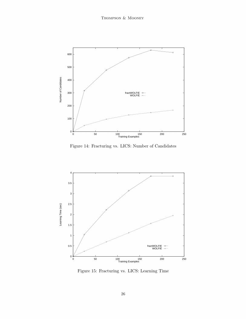
In addition, the number of initial candidate lexicon entries from which to choose ismuch larger for fracturing than our LICS method, as shown in Figure 14. This is true eventhough we sampled the same number of representations as pairs for LICS, because thereare a larger number of fractures for an arbitrary representation than the number of LICSfor an arbitrary pair. Finally, Wolfie’s learning time when using fracturing is greater thanthat when using LICS, as shown in Figure 15, where the CPU time is shown in seconds.

In summary, these differences show the utility of LICS as a method for generatingcandidates: a more thorough method does not result in better performance, and also resultsin longer learning times. One could claim that we are handicapping fracturing since we areonly sampling representations for fracturing. This may indeed help the accuracy, but thelearning time and the number of candidates would likely suffer even further. In a domainwith larger representations, the differences in learning time would be even more dramatic.

5.2 Artificial Data

The previous section showed that Wolfie successfully learns lexicons for a natural corpusand a realistic task. However, this demonstrates success on only a relatively small corpusand with one representation formalism. We now show that our algorithm scales up wellwith more lexicon items to learn, more ambiguity, and more synonymy. These factors are

25

Thompson & Mooney

0

100

200

300

400

500

600

0 50 100 150 200 250

Num

ber

of C

andi

date

s

Training Examples

fractWOLFIEWOLFIE

Figure 14: Fracturing vs. LICS: Number of Candidates

0

0.5

1

1.5

2

2.5

3

3.5

4

0 50 100 150 200 250

Lear

ning

Tim

e (s

ec)

Training Examples

fractWOLFIEWOLFIE

Figure 15: Fracturing vs. LICS: Learning Time

26


difficult to control when using real data as input. Also, there are no large corpora availablethat are annotated with semantic parses. We therefore present experimental results on anartificial corpus. In this corpus, both the sentences and their representations are completelyartificial, and the sentence representation is a variable-free representation, as suggested bythe work of Jackendoff (1990) and others.

For each corpus discussed below, a random lexicon mapping words to simulated meaningswas first constructed.11 This original lexicon was then used to generate a corpus of randomutterances each paired with a meaning representation. After using this corpus as input toWolfie

12, the learned lexicon was compared to the original lexicon, and weighted precisionand weighted recall of the learned lexicon were measured. Precision measures the percentageof the lexicon entries (i.e., word-meaning pairs) that the system learns that are correct.Recall measures the percentage of the lexicon entries in the hand-built lexicon that arecorrectly learned by the system:

precision =# correct pairs# pairs learned

recall =# correct pairs

# pairs in hand-built lexicon.

To get weighted precision and recall measures, we then weight the results for each pairby the word’s frequency in the entire corpus (not just the training corpus). This modelshow likely we are to have learned the correct meaning for an arbitrarily chosen word in thecorpus.

We generated several lexicons and associated corpora, varying the ambiguity rate (num-ber of meanings per word) and synonymy rate (number of words per meaning), as in Siskind(1996). Meaning representations were generated using a set of “conceptual symbols” thatcombined to form the meaning for each word. The number of conceptual symbols used ineach lexicon will be noted when we describe each corpus below. In each lexicon, 47.5%of the senses were variable-free to simulate noun-like meanings, and 47.5% contained fromone to three variables to denote open argument positions to simulate verb-like meanings.The remainder of the words (the remaining 5%) had the empty meaning to simulate func-tion words. In addition, the functors in each meaning could have a depth of up to twoand an arity of up to two. An example noun-like meaning is f23(f2(f14)), and a verb-meaning f10(A,f15(B)); the conceptual symbols in this example are f23, f2, f14, f10,and f15. By using these multi-level meaning representations we demonstrate the learningof more complex representations than those in the geography database domain: none of thehand-built meanings for phrases in that lexicon had functors embedded in arguments. Weused a grammar to generate utterances and their meanings from each original lexicon, withterminal categories selected using a distribution based on Zipf’s Law (Zipf, 1949). UnderZipf’s Law, the occurrence frequency of a word is inversely proportional to its ranking byoccurrence.

We started with a baseline corpus generated from a lexicon of 100 words using 25 concep-tual symbols and no ambiguity or synonymy; 1949 sentence-meaning pairs were generated.

11. Thanks to Jeff Siskind for the initial corpus generation software, which we enhanced for these tests.12. In these tests, we allowed Wolfie to learn phrases of up to length two.

27

Thompson & Mooney

0

10

20

30

40

50

60

70

80

90

100

0 200 400 600 800 1000 1200 1400 1600 1800

Acc

urac

y

Training Examples

PrecisionRecall

Figure 16: Baseline Artificial Corpus

We split this into five training sets of 1700 sentences each. Figure 16 shows the weightedprecision and recall curves for this initial test. This demonstrates good scalability to aslightly larger corpus and lexicon than that of the U.S. geography query domain.

A second corpus was generated from a second lexicon, also of 100 words using 25 concep-tual symbols, but increasing the ambiguity to 1.25 meanings per word. This time, 1937 pairswere generated and the corpus split into five sets of 1700 training examples each. Weightedprecision at 1650 examples drops to 65.4% from the previous level of 99.3%, and weightedrecall to 58.9% from 99.3%. The full learning curve is shown in Figure 17. A quick compari-son to Siskind’s performance on this corpus confirmed that his system achieved comparableperformance, showing that with current methods, this is close to the best performance thatwe are able to obtain on this more difficult corpus. One possible explanation for the smallerperformance difference between the two systems on this corpus versus the geography do-main is that in this domain, the correct meaning for a word is not necessarily the most“general,” in terms of number of vertices, of all its candidate meanings. Therefore, thegenerality portion of the heuristic may negatively influence the performance of Wolfie inthis domain.

Finally, we show the change in performance with increasing ambiguity and increasingsynonymy, holding the number of words and conceptual symbols constant. Figure 18 showsthe weighted precision and recall with 1050 training examples for increasing levels of am-biguity, holding the synonymy level constant. Figure 19 shows the results at increasinglevels of synonymy, holding ambiguity constant. Increasing the level of synonymy does noteffect the results as much as increasing the level of ambiguity, which is as we expected.Holding the corpus size constant but increasing the number of competing meanings for aword increases the number of candidate meanings created by Wolfie while decreasing theamount of evidence available for each meaning (e.g., the first component of the heuristic

28


0

10

20

30

40

50

60

70

0 200 400 600 800 1000 1200 1400 1600 1800

Acc

urac

y

Training Examples

PrecisionRecall

Figure 17: A More Ambiguous Artificial Corpus

60

65

70

75

80

85

90

95

100

1 1.25 1.5 1.75 2

Acc

urac

y

Number of Meanings per Word

RecallPrecision

Figure 18: Increasing the Level of Ambiguity

measure) and makes the learning task more difficult. On the other hand, increasing thelevel of synonymy does not have the potential to mislead the learner.

The number of training examples required to reach a certain level of accuracy is alsoinformative. In Table 4, we show the point at which a standard precision of 75% was first

29

Thompson & Mooney

80

85

90

95

100

1 1.25 1.5 1.75 2

Acc

urac

y

Number of Words per Meaning

RecallPrecision

Figure 19: Increasing the Level of Synonymy

Ambiguity Level Number of Examples1.0 1501.25 4502.0 1450

Table 4: Number of Examples to Reach 75% Precision

reached for each level of ambiguity. Note, however, that we only measured accuracy aftereach set of 100 training examples, so the numbers in the table are approximate.

We performed a second test of scalability on two corpora generated from lexicons anorder of magnitude larger than those in the above tests. In these tests, we use a lexiconcontaining 1000 words and using 250 conceptual symbols. We generated both a corpus withno ambiguity, and one from a lexicon with ambiguity and synonymy similar to that foundin the WordNet database (Beckwith, Fellbaum, Gross, & Miller, 1991); the ambiguity thereis approximately 1.68 meanings per word and the synonymy 1.3 words per meaning. Thesecorpora contained 9904 (no ambiguity) and 9948 examples, respectively, and we split thedata into five sets of 9000 training examples each. For the easier large corpus, the maximumaverage of weighted precision and recall was 85.6%, at 8100 training examples, while for theharder corpus, the maximum average was 63.1% at 8600 training examples.

6. Active Learning

As indicated in the previous sections, we have built an integrated system for languageacquisition that is flexible and useful. However, a major difficulty remains: the constructionof training corpora. Though annotating sentences is still arguably less work than building

30


Apply the learner to n bootstrap examples, creating a classifier.Until no examples remain or the annotator is unwilling to label more examples, do:

Use most recently learned classifier to annotate each unlabeled instance.Find the k instances with the lowest annotation certainty.Annotate these instances.Train the learner on the bootstrap examples and all examples annotated so far.

Figure 20: Selective Sampling Algorithm

an entire system by hand, the annotation task is also time-consuming and error-prone.Further, the training pairs often contain redundant information. We would like to minimizethe amount of annotation required while still maintaining good generalization accuracy.

To do this, we turned to methods in active learning. Active learning is a research areain machine learning that features systems that automatically select the most informativeexamples for annotation and training (Angluin, 1988; Seung, Opper, & Sompolinsky, 1992),rather than relying on a benevolent teacher or random sampling. The primary goal ofactive learning is to reduce the number of examples that the system is trained on, whilemaintaining the accuracy of the acquired information. Active learning systems may con-struct their own examples, request certain types of examples, or determine which of a setof unsupervised examples are most usefully labeled. The last approach, selective sampling(Cohn et al., 1994), is particularly attractive in natural language learning, since there is anabundance of text, and we would like to annotate only the most informative sentences. Formany language learning tasks, annotation is particularly time-consuming since it requiresspecifying a complex output rather than just a category label, so reducing the number oftraining examples required can greatly increase the utility of learning.

In this section, we explore the use of active learning, specifically selective sampling, forlexicon acquisition, and demonstrate that with active learning, fewer examples are requiredto achieve the same accuracy obtained by training on randomly chosen examples.

The basic algorithm for selective sampling is relatively simple. Learning begins with asmall pool of annotated examples and a large pool of unannotated examples, and the learnerattempts to choose the most informative additional examples for annotation. Existing workin the area has emphasized two approaches, certainty-based methods (Lewis & Catlett,1994), and committee-based methods (McCallum & Nigam, 1998; Freund, Seung, Shamir,& Tishby, 1997; Liere & Tadepalli, 1997; Dagan & Engelson, 1995; Cohn et al., 1994); wefocus here on the former.

In the certainty-based paradigm, a system is trained on a small number of annotatedexamples to learn an initial classifier. Next, the system examines unannotated examples,and attaches certainties to the predicted annotation of those examples. The k examples withthe lowest certainties are then presented to the user for annotation and retraining. Manymethods for attaching certainties have been used, but they typically attempt to estimatethe probability that a classifier consistent with the prior training data will classify a newexample correctly.

31

Thompson & Mooney

Learn a lexicon with the examples annotated so far1) For each phrase in an unannotated sentence:

If it has entries in the learned lexicon thenits certainty is the average of the heuristic values of those entries

Else, if it is a one-word phrase thenits certainty is zero

2) To rank sentences use:Total certainty of phrases from step 1

# of phrases counted in step 1

Figure 21: Active Learning for Wolfie

Figure 20 presents abstract pseudocode for certainty-based selective sampling. In anideal situation, the batch size, k, would be set to one to make the most intelligent decisionsin future choices, but for efficiency reasons in retraining batch learning algorithms, it isfrequently set higher. Results on a number of classification tasks have demonstrated thatthis general approach is effective in reducing the need for labeled examples (see citationsabove).

Applying certainty-based sample selection to Wolfie requires determining the certaintyof a complete annotation of a potential new training example, despite the fact that individuallearned lexical entries and parsing operators perform only part of the overall annotation task.Therefore, our general approach is to compute certainties for pieces of an example, in ourcase, phrases, and combine these to obtain an overall certainty for an example. Since lexiconentries contain no explicit uncertainty parameters, we used Wolfie’s heuristic measure toestimate uncertainty.

To choose the sentences to be annotated in each round, we first bootstrapped an initiallexicon from a small corpus, keeping track of the heuristic values of the learned items.Then, for each unannotated sentence, we took an average of the heuristic values of thelexicon entries learned for phrases in that sentence, giving a value of zero to unknownwords but eliminating from consideration any words that we assume are known in advance,such as database constants. Thus, longer sentences with only a few known phrases wouldhave a lower certainty than shorter sentences with the same number of known phrases; thisis desirable since longer sentences will be more informative from a lexicon learning pointof view. The sentences with the lowest values were chosen for annotation, added to thebootstrap corpus, and a new lexicon learned. Our technique is summarized in Figure 21.

To evaluate our technique, we compared active learning to learning from randomly se-lected examples, again measuring the effectiveness of learned lexicons as background knowl-edge for Chill. We again used the (smaller) U.S. Geography corpus, as in the originalWolfie tests, using the lexicons as background knowledge during parser acquisition (andusing the same examples for parser acquisition).

For each trial in the following experiments, we first randomly divide the data into atraining and test set. Then, n = 25 bootstrap examples are randomly selected from the

32


0

20

40

60

80

100

0 50 100 150 200 250

Acc

urac

y

Training Examples

WOLF+activeWOLFIEGeobase

Figure 22: Using Lexicon Certainty for Active Learning

training examples and in each step of active learning, the least certain k = 10 examplesof the remaining training examples are selected and added to the training set. The resultof learning on this set is evaluated after each step. The accuracy of the resulting learnedparsers was compared to the accuracy of those learned using randomly chosen examples tolearn lexicons and parsers, as in Section 5; in other words, we can think of the k examplesin each round as being chosen randomly.

Figure 22 shows the accuracy on unseen data of parsers learned using the lexicons learnedby Wolfie when examples are chosen randomly and actively. There is an annotationsavings of around 50 examples by using active learning: the maximum accuracy is reachedafter 175 examples, versus 225 with random examples. The advantage of using activelearning is clear from the beginning, though the differences between the two curves are onlystatistically significant at 175 training examples. Since we are learning both lexicons andparsers, but only choosing examples based on Wolfie’s certainty measures, the boost couldbe improved even further if Chill had a say in the examples chosen. See Thompson, Califf,and Mooney (1999) for a description of active learning for Chill.

7. Related Work

In this section, we divide the previous research on related topics into the areas of lexiconacquisition and active learning.

7.1 Lexicon Acquisition

Work on automated lexicon and language acquisition dates back to Siklossy (1972), whodemonstrated a system that learned transformation patterns from logic back to natural

33

Thompson & Mooney

language. As already noted, the most closely related work is that of Jeff Siskind, which wedescribed briefly in Section 2 and whose system we ran comparisons to in Section 5. Ourdefinition of the learning problem can be compared to his “mapping problem” (Siskind,1993). That formulation differs from ours in several respects. First, his sentence repre-sentations are terms instead of trees. However, as shown in Figure 7, terms can also berepresented as trees that conform to our formalism with some minor additions. Next, hisnotion of interpretation does involve a type of tree, but carries the entire representation ofa sentence up to the root. Also, it is not clear how he would handle quantified variablesin the representation of sentences. Skolemization is possible, but then generalization acrosssentences would require special handling. We make the single-use assumption and he doesnot. Another difference is our bias towards a minimal number of lexicon entries, while heattempts to find a monosemous lexicon. His later work (Siskind, 2000) relaxes this to allowambiguity and noise, but still biases towards minimizing ambiguity. However, his formaldefinition does not explicitly allow lexical ambiguity, but handles it in a heuristic manner.This, though, may lead to more robustness than our method in the face of noise. Finally,our definition allows phrasal lexicon entries.

Siskind’s work on this topic has explored many different variations along a continuum ofusing many constraints but requiring more time to incorporate each new example (Siskind,1993), versus few constraints but requiring more training data (Siskind, 1996). Thus, per-haps his earlier systems would have been able to learn the lexicons of Section 5 morequickly; but crucially those systems did not allow lexical ambiguity, and thus also maynot have learned as accurate a lexicon. More detailed comparisons to such versions of thesystem are outside the scope of this paper. Our goal with Wolfie is to learn a possiblyambiguous lexicon from as few examples as possible, and we thus made comparisons alongthis dimension alone.

Siskind’s approach, like ours, takes into account constraints between word meaningsthat are justified by the exclusivity and compositionality assumptions. His approach issomewhat more general in that it handles noise and referential uncertainty (uncertaintyabout the meaning of a sentence and thus multiple possible candidates), while ours isspecialized for applications where the meaning (or meanings) is known. The experimentalresults in Section 5 demonstrate the advantage of our method for such an application. He hasdemonstrated his system to be capable of learning reasonably accurate lexicons from large,ambiguous, and noisy artificial corpora, but this accuracy is only assured if the learningalgorithm converges, which did not occur for our smaller corpus in the experiments we ran.Also, as already noted, his system operates in an incremental or on-line fashion, discardingeach sentence as it processes it, while ours is batch. In addition, his search for word meaningsproceeds in two stages, as discussed in Section 2.2. By using common substructures, wecombine these two stages in Wolfie. Both systems do have greedy aspects, ours in thechoice of the next best lexical entry, his in the choice to discard utterances as noise or createa homonymous lexical entry. Finally, his system does not compute statistical correlationsbetween words and their possible meanings, while ours does.

Besides Siskind’s work, there are others who approach the problem from a cognitiveperspective. For example, De Marcken (1994) also uses child language learning as a mo-tivation, but approaches the segmentation problem instead of the learning of semantics.For training input, he uses a flat list of tokens for semantic representations, but does not

34


segment sentences into words. He uses a variant of expectation-maximization (Dempster,Laird, & Rubin, 1977), together with a form of parsing and dictionary matching techniques,to segment the sentences and associate the segments with their most likely meaning. Onthe Childes corpus, the algorithm achieves very high precision, but recall is not provided.

Others taking the cognitive approach demonstrate language understanding by the abilityto carry out some task such as parsing. For example, Nenov and Dyer (1994) describe aneural network model to map between visual and verbal-motor commands, and Colungaand Gasser (1998) use neural network modeling techniques for learning spatial concepts.Feldman and his colleagues at Berkeley (Feldman, Lakoff, & Shastri, 1995) are activelypursuing cognitive models of the acquisition of semantic concepts. Another Berkeley effort,the system by Regier (1996) is given examples of pictures paired with natural languagedescriptions that apply to the picture, and learns to judge whether a new sentence is trueof a given picture.

Similar work by Suppes, Liang, and Bottner (1991) uses robots to demonstrate lexi-con learning. A robot is trained on cognitive and perceptual concepts and their associatedactions, and learns to execute simple commands. Along similar lines, Tishby and Gorin(1994) have a system that learns associations between words and actions, but they use astatistical framework to learn these associations, and do not handle structured representa-tions. Similarly, Oates, Eyler-Walker, and Cohen (1999) discuss the acquisition of lexicalhierarchies and their associated meaning as defined by the sensory environment of a robot.

The problem of automatic construction of translation lexicons (Smadja, McKeown, &Hatzivassiloglou, 1996; Melamed, 1995; Wu & Xia, 1995; Kumano & Hirakawa, 1994; Cati-zone, Russell, & Warwick, 1993; Gale & Church, 1991; Brown & et al., 1990) has a definitionsimilar to our own. While most of these methods also compute association scores betweenpairs (in their case, word-word pairs) and use a greedy algorithm to choose the best trans-lation(s) for each word, they do not take advantage of the constraints between pairs. Oneexception is Melamed (2000); however, his approach does not allow for phrases in the lex-icon or for synonymy within one text segment, while ours does. Also, Yamazaki, Pazzani,and Merz (1995) learn both translation rules and semantic hierarchies from parsed parallelsentences in Japanese and English. Of course, the main difference between this body ofwork and this paper is that we map words to semantic structures, not to other words.

As mentioned in the introduction, there is also a large body of work on learning lexicalsemantics but using different problem formulations than our own. For example, Collins andSinger (1999), Riloff and Jones (1999), Roark and Charniak (1998), and Schneider (1998)define semantic lexicons as a grouping of words into semantic categories, and in the lattercase, add relational information. The result is typically applied as a semantic lexicon forinformation extraction or entity tagging. Pedersen and Chen (1995) describe a methodfor acquiring syntactic and semantic features of an unknown word, assuming access to aninitial concept hierarchy, but they give no experimental results. Many systems (Fukumoto &Tsujii, 1995; Haruno, 1995; Johnston, Boguraev, & Pustejovsky, 1995; Webster & Marcus,1995) focus only on acquisition of verbs or nouns, rather than all types of words. Also, theauthors just named either do not experimentally evaluate their systems, or do not show theusefulness of the learned lexicons for a specific application.

Several authors (Rooth, Riezler, Prescher, Carroll, & Beil, 1999; Collins, 1997; Ribas,1994; Manning, 1993; Resnik, 1993; Brent, 1991) discuss the acquisition of subcategoriza-

35

Thompson & Mooney

tion information for verbs, and others describe work on learning selectional restrictions(Manning, 1993; Brent, 1991). Both of these are different from the information requiredfor mapping to semantic representation, but could be useful as a source of information tofurther constrain the search. Li (1998) further expands on the subcategorization work byinducing clustering information. Finally, several systems (Knight, 1996; Hastings, 1996;Russell, 1993) learn new words from context, assuming that a large initial lexicon andparsing system are already available.

Another related body of work is grammar acquisition, especially those areas that tightlyintegrate the grammar with a lexicon, such as with Categorial Grammars (Retore & Bonato,2001; Dudau-Sofronie, Tellier, & Tommasi, 2001; Watkinson & Manandhar, 1999). Thetheory of Categorial Grammar also has ties with lexical semantics, but these semanticshave not often been used for inference in support of high-level tasks such as databaseretrieval. While learning syntax and semantics together is arguably a more difficult task,the aforementioned work has not been evaluated on large corpora, presumably primarilydue to the difficulty of annotation.

7.2 Active Learning

With respect to additional active learning techniques, Cohn et al. (1994) were among thefirst to discuss certainty-based active learning methods in detail. They focus on a neuralnetwork approach to active learning in a version-space of concepts. Only a few of theresearchers applying machine learning to natural language processing have utilized activelearning (Hwa, 2001; Schohn & Cohn, 2000; Tong & Koller, 2000; Thompson et al., 1999;Argamon-Engelson & Dagan, 1999; Liere & Tadepalli, 1997; Lewis & Catlett, 1994), andthe majority of these have addressed classification tasks such as part of speech taggingand text categorization. For example, Liere and Tadepalli (1997) apply active learningwith committees to the problem of text categorization. They show improvements withactive learning similar to those that we obtain, but use a committee of Winnow-basedlearners on a traditional classification task. Argamon-Engelson and Dagan (1999) alsoapply committee-based learning to part-of-speech tagging. In their work, a committee ofhidden Markov models is used to select examples for annotation. Lewis and Catlett (1994)use heterogeneous certainty-based methods, in which a simple classifier is used to selectexamples that are then annotated and presented to a more powerful classifier.

However, many language learning tasks require annotating natural language text witha complex output, such as a parse tree, semantic representation, or filled template. Theapplication of active learning to tasks requiring such complex outputs has not been wellstudied, the exceptions being Hwa (2001), Soderland (1999), Thompson et al. (1999). Thelatter two include work on active learning applied to information extraction, and Thompsonet al. (1999) includes work on active learning for semantic parsing. Hwa (2001) describesan interesting method for evaluating a statistical parser’s uncertainty, when applied forsyntactic parsing.

8. Future Work

Although Wolfie’s current greedy search method has performed quite well, a better searchheuristic or alternative search strategy could result in improvements. We should also more

36


thoroughly evaluate Wolfie’s ability to learn long phrases, as we restricted this ability inthe evaluations here. Another issue is robustness in the face of noise. The current algorithmis not guaranteed to learn a correct lexicon in even a noise-free corpus. The addition of noisecomplicates an analysis of circumstances in which mistakes are likely to happen. Furthertheoretical and empirical analysis of these issues is warranted.

Referential uncertainty could be handled, with an increase in complexity, by formingLICS from more pairs of representations with which a phrase appears, but not betweenalternative representations of the same sentence. Then, once a pair is added to the lexicon,for each sentence containing that word, representations can be eliminated if they do notcontain the learned meaning, provided another representation does contain it (thus allowingfor lexical ambiguity). We plan to flesh this out and evaluate the results.

A different avenue of exploration is to apply Wolfie to a corpus of sentences pairedwith the more common query language, SQL. Such corpora should be easily constructibleby recording queries submitted to existing SQL applications along with their English forms,or translating existing lists of SQL queries into English (presumably an easier direction totranslate). The fact that the same training data can be used to learn both a semanticlexicon and a parser also helps limit the overall burden of constructing a complete naturallanguage interface.

With respect to active learning, experiments on additional corpora are needed to testthe ability of our approach to reduce annotation costs in a variety of domains. It wouldalso be interesting to explore active learning for other natural language processing problemssuch as syntactic parsing, word-sense disambiguation, and machine translation.

Our current results have involved a certainty-based approach; however, proponents ofcommittee-based approaches have convincing arguments for their theoretical advantages.Our initial attempts at adapting committee-based approaches to our systems were not verysuccessful; however, additional research on this topic is indicated. One critical problem isobtaining diverse committees that properly sample the version space (Cohn et al., 1994).

9. Conclusions

Acquiring a semantic lexicon from a corpus of sentences labeled with representations oftheir meaning is an important problem that has not been widely studied. We present both aformalism of the learning problem and a greedy algorithm to find an approximate solution toit. Wolfie demonstrates that a fairly simple, greedy, symbolic learning algorithm performswell on this task and obtains performance superior to a previous lexicon acquisition systemon a corpus of geography queries. Our results also demonstrate that our methods extendto a variety of natural languages besides English, and that they scale fairly well to larger,more difficult corpora.

Active learning is a new area of machine learning that has been almost exclusivelyapplied to classification tasks. We have demonstrated its successful application to morecomplex natural language mappings from phrases to semantic meanings, supporting theacquisition of lexicons and parsers. The wealth of unannotated natural language data,along with the difficulty of annotating such data, make selective sampling a potentiallyinvaluable technique for natural language learning. Our results on realistic corpora indicatethat example annotations savings as high as 22% can be achieved by employing active

37

Thompson & Mooney

sample selection using only simple certainty measures for predictions on unannotated data.Improved sample selection methods and applications to other important language problemshold the promise of continued progress in using machine learning to construct effectivenatural language processing systems.

Most experiments in corpus-based natural language have presented results on somesubtask of natural language, and there are few results on whether the learned subsystemscan be successfully integrated to build a complete NLP system. The experiments presentedin this paper demonstrated how two learning systems, Wolfie and Chill, were successfullyintegrated to learn a complete NLP system for parsing database queries into executablelogical form given only a single corpus of annotated queries, and further demonstrated thepotential of active learning to reduce the annotation effort for learning for NLP.

Acknowledgments

We would like to thank Jeff Siskind for providing us with his software, and for all his helpin adapting it for use with our corpus. Thanks also to Agapito Sustaita, Esra Erdem,and Marshall Mayberry for their translation efforts, and to the three anonymous reviewersfor their comments which helped improve the paper. This research was supported by theNational Science Foundation under grants IRI-9310819 and IRI-9704943.

References

Anderson, J. R. (1977). Induction of augmented transition networks. Cognitive Science, 1,125–157.

Angluin, D. (1988). Queries and concept learning. Machine Learning, 2, 319–342.

Argamon-Engelson, S., & Dagan, I. (1999). Committee-based sample selection for proba-bilistic classifiers. Journal of Artificial Intelligence Research, 11, 335–360.

Beckwith, R., Fellbaum, C., Gross, D., & Miller, G. (1991). WordNet: A lexical databaseorganized on psycholinguistic principles. In Zernik, U. (Ed.), Lexical Acquisition:Exploiting On-Line Resources to Build a Lexicon, pp. 211–232. Lawrence Erlbaum,Hillsdale, NJ.

Borland International (1988). Turbo Prolog 2.0 Reference Guide. Borland International,Scotts Valley, CA.

Brent, M. (1991). Automatic acquisition of subcategorization frames from untagged text.In Proceedings of the 29th Annual Meeting of the Association for Computational Lin-guistics (ACL-91), pp. 209–214.

Brown, P., & et al. (1990). A statistical approach to machine translation. ComputationalLinguistics, 16 (2), 79–85.

Catizone, R., Russell, G., & Warwick, S. (1993). Deriving translation data from bilingualtexts. In Proceedings of the First International Lexical Acquisition Workshop.

38


Cohn, D., Atlas, L., & Ladner, R. (1994). Improving generalization with active learning.Machine Learning, 15 (2), 201–221.

Collins, M., & Singer, Y. (1999). Unsupervised models for named entity classification. InProceedings of the Conference on Empirical Methods in Natural Language Processingand Very Large Corpora (EMNLP/VLC-99) University of Maryland.

Collins, M. J. (1997). Three generative, lexicalised models for statistical parsing. In Pro-ceedings of the 35th Annual Meeting of the Association for Computational Linguistics(ACL-97), pp. 16–23.

Colunga, E., & Gasser, M. (1998). Linguistic relativity and word acquisition: a com-putational approach. In Proceedings of the Twenty First Annual Conference of theCognitive Science Society, pp. 244–249.

Dagan, I., & Engelson, S. P. (1995). Committee-based sampling for training probabilis-tic classifiers. In Proceedings of the Twelfth International Conference on MachineLearning (ICML-95), pp. 150–157 San Francisco, CA. Morgan Kaufman.

De Marcken, C. (1994). The acquisition of a lexicon from paired phoneme sequences andsemantic representations. In Lecture Notes in Computer Science, Vol. 862, pp. 66–77.Springer-Verlag.

Dempster, A., Laird, N., & Rubin, D. (1977). Maximum likelihood from incomplete datavia the EM algorithm. Journal of the Royal Statistical Society B, 39, 1–38.

Dudau-Sofronie, Tellier, & Tommasi (2001). Learning categorial grammars from semantictypes. In Proceedings of the 13th Amsterdam Colloquium, pp. 79–84.

Feldman, J., Lakoff, G., & Shastri, L. (1995). The neural theory of language projecthttp://www.icsi.berkeley.edu/ntl. International Computer Science Institute, Universityof California, Berkeley, CA.

Fillmore, C. (1968). The case for case. In Bach, E., & Harms, R. T. (Eds.), Universals inLinguistic Theory. Holt, Reinhart and Winston, New York.

Fillmore, C. (1988). The mechanisms of “Construction Grammar”. In Axmaker, S., Jaisser,A., & Singmeister, H. (Eds.), Proceedings of the Fourteenth Annual Meeting of theBerkeley Linguistics Society, pp. 35–55 Berkeley, CA.

Fisher, D. H. (1987). Knowledge acquisition via incremental conceptual clustering. MachineLearning, 2, 139–172.

Freund, Y., Seung, H. S., Shamir, E., & Tishby, N. (1997). Selective sampling using thequery by committee algorithm. Machine Learning, 28, 133–168.

Fukumoto, F., & Tsujii, J. (1995). Representation and acquisition of verbal polysemy. InPapers from the 1995 AAAI Symposium on the Representation and Acquisition ofLexical Knowledge: Polysemy, Ambiguity, and Generativity, pp. 39–44 Stanford, CA.

39

Thompson & Mooney

Gale, W., & Church, K. (1991). Identifying word correspondences in parallel texts. InProceedings of the Fourth DARPA Speech and Natural Language Workshop.

Garey, M., & Johnson, D. (1979). Computers and Intractability: A Guide to the Theory ofNP-Completeness. Freeman, New York, NY.

Goldberg, A. (1995). Constructions: A Construction Grammar Approach to ArgumentStructure. The University of Chicago Press.

Grefenstette, G. (1994). Sextant: Extracting semantics from raw text, implementationdetails. Integrated Computer-Aided Engineering, 6 (4).

Haas, J., & Jayaraman, B. (1997). From context-free to definite-clause grammars: a type-theoretic approach. Journal of Logic Programming, 30 (1), 1–23.

Haruno, M. (1995). A case frame learning method for Japanese polysemous verbs. InPapers from the 1995 AAAI Symposium on the Representation and Acquisition ofLexical Knowledge: Polysemy, Ambiguity, and Generativity, pp. 45–50 Stanford, CA.

Hastings, P. (1996). Implications of an automatic lexical acquisition mechanism. InWermter, S., Riloff, E., & Scheler, C. (Eds.), Connectionist, Statistical, and Sym-bolic Approaches to Learning for natural language processing. Springer-Verlag, Berlin.

Hwa, R. (2001). On minimizing training corpus for parser acquisition. In Proceedings ofthe Fifth Computational Natural Language Learning Workshop.

Jackendoff, R. (1990). Semantic Structures. The MIT Press, Cambridge, MA.

Johnston, M., Boguraev, B., & Pustejovsky, J. (1995). The acquisition and interpretation ofcomplex nominals. In Papers from the 1995 AAAI Symposium on the Representationand Acquisition of Lexical Knowledge: Polysemy, Ambiguity, and Generativity, pp.69–74 Stanford, CA.

Knight, K. (1996). Learning word meanings by instruction. In Proceedings of the ThirteenthNational Conference on Artificial Intelligence (AAAI-96), pp. 447–454 Portland, Or.

Kohavi, R., & John, G. (1995). Automatic parameter selection by minimizing estimatederror. In Proceedings of the Twelfth International Conference on Machine Learning(ICML-95), pp. 304–312 Tahoe City, CA.

Kumano, A., & Hirakawa, H. (1994). Building an MT dictionary from parallel texts basedon linguistic and statistical information. In Proceedings of the Fifteenth InternationalConference on Computational Linguistics, pp. 76–81.

Lavrac, N., & Dzeroski, S. (1994). Inductive Logic Programming: Techniques and Applica-tions. Ellis Horwood.

Lewis, D. D., & Catlett, J. (1994). Heterogeneous uncertainty sampling for supervisedlearning. In Proceedings of the Eleventh International Conference on Machine Learn-ing (ICML-94), pp. 148–156 San Francisco, CA. Morgan Kaufman.

40


Li, H. (1998). A probabilistic approach to lexical semantic knowledge acquisition and struc-tural disambiguation. Ph.D. thesis, University of Tokyo.

Liere, R., & Tadepalli, P. (1997). Active learning with committees for text categorization. InProceedings of the Fourteenth National Conference on Artificial Intelligence (AAAI-97), pp. 591–596 Providence, RI.

Manning, C. D. (1993). Automatic acquisition of a large subcategorization dictionary fromcorpora. In Proceedings of the 31st Annual Meeting of the Association for Computa-tional Linguistics (ACL-93), pp. 235–242 Columbus, OH.

McCallum, A. K., & Nigam, K. (1998). Employing EM and pool-based active learningfor text classification. In Proceedings of the Fifteenth International Conference onMachine Learning (ICML-98), pp. 350–358 Madison, WI. Morgan Kaufman.

Melamed, I. D. (1995). Automatic evaluation and uniform filter cascades for inducing n-besttranslation lexicons. In Proceedings of the Third Workshop on Very Large Corpora.

Melamed, I. D. (2000). Models of translational equivalence among words. ComputationalLinguistics, 26 (2), 221–249.

Muggleton, S. (Ed.). (1992). Inductive Logic Programming. Academic Press, New York,NY.

Muggleton, S. (1995). Inverse entailment and Progol. New Generation Computing Journal,13, 245–286.

Muggleton, S., & Feng, C. (1990). Efficient induction of logic programs. In Proceedings ofthe First Conference on Algorithmic Learning Theory Tokyo, Japan. Ohmsha.

Nenov, V. I., & Dyer, M. G. (1994). Perceptually grounded language learning: Part 2–DETE: A neural/procedural model. Connection Science, 6 (1), 3–41.

Oates, T., Eyler-Walker, Z., & Cohen, P. (1999). Using syntax to learn semantics: anexperiment in language acquisition with a mobile robot. Tech. rep. 99-35, Universityof Massachusetts, Computer Science Department.

Partee, B., Meulen, A., & Wall, R. (1990). Mathematical Methods in Linguistics. KluwerAcademic Publishers, Dordrecht, The Netherlands.

Pedersen, T., & Chen, W. (1995). Lexical acquisition via constraint solving. In Papersfrom the 1995 AAAI Symposium on the Representation and Acquisition of LexicalKnowledge: Polysemy, Ambiguity, and Generativity, pp. 118–122 Stanford, CA.

Plotkin, G. D. (1970). A note on inductive generalization. In Meltzer, B., & Michie, D.(Eds.), Machine Intelligence (Vol. 5). Elsevier North-Holland, New York.

Rayner, M., Hugosson, A., & Hagert, G. (1988). Using a logic grammar to learn a lexicon.Tech. rep. R88001, Swedish Institute of Computer Science.

41

Thompson & Mooney

Regier, T. (1996). The human semantic potential: spatial language and constrained connec-tionism. MIT Press.

Resnik, P. (1993). Selection and information: a class-based approach to lexical relationships.Ph.D. thesis, University of Pennsylvania, CIS Department.

Retore, C., & Bonato, R. (2001). Learning rigid lambek grammars and minimalist grammarsfrom structured sentences. In Proceedings of the Third Learning Language in LogicWorkshop Strasbourg, France.

Ribas, F. (1994). An experiment on learning appropriate selectional restrictions from aparsed corpus. In Proceedings of the Fifteenth International Conference on Computa-tional Linguistics, pp. 769–774.

Riloff, E., & Jones, R. (1999). Learning dictionaries for information extraction by multi-level bootstrapping. In Proceedings of the Sixteenth National Conference on ArtificialIntelligence (AAAI-99), pp. 1044–1049 Orlando, FL.

Roark, B., & Charniak, E. (1998). Noun-phrase co-occurrence statistics for semi-automaticsemantic lexicon construction. In Proceedings of the 36th Annual Meeting of theAssociation for Computational Linguistics and COLING-98 (ACL/COLING-98), pp.1110–1116.

Rooth, M., Riezler, S., Prescher, D., Carroll, G., & Beil, F. (1999). Inducing a semanticallyannotated lexicon via EM-based clustering. In Proceedings of the 37th Annual Meetingof the Association for Computational Linguistics, pp. 104–111.

Russell, D. (1993). Language Acquisition in a Unification-Based Grammar Processing Sys-tem Using a Real World Knowledge Base. Ph.D. thesis, University of Illinois, Urbana,IL.

Schank, R. C. (1975). Conceptual Information Processing. North-Holland, Oxford.

Schneider, R. (1998). A lexically-intensive algorithm for domain-specific knowledge acquisi-tion. In Proceedings of the Joint Conference on New Methods in Language Processingand Computational Natural Language Learning, pp. 19–28.

Schohn, G., & Cohn, D. (2000). Less is more: Active learning with support vector ma-chines. In Proceedings of the Seventeenth International Conference on Machine Learn-ing (ICML-2000), pp. 839–846 Stanford, CA.

Sebillot, P., Bouillon, P., & Fabre, C. (2000). Inductive logic programming for corpus-basedacquisition of semantic lexicons. In Proceedings of 2nd Learning Language in Logic(LLL) Workshop Lisbon, Portugal.

Seung, H. S., Opper, M., & Sompolinsky, H. (1992). Query by committee. In Proceedingsof the ACM Workshop on Computational Learning Theory Pittsburgh, PA.

Siklossy, L. (1972). Natural language learning by computer. In Simon, H. A., & Siklossy,L. (Eds.), Representation and meaning: Experiments with Information ProcesssingSystems. Prentice Hall, Englewood Cliffs, NJ.

42


Siskind, J. M. (2000). Learning word-to-meaning mappings. In Broeder, P., & Murre, J.(Eds.), Models of Language Acquisition: Inductive and Deductive Approaches. OxfordUniversity Press.

Siskind, J. M. (1992). Naive Physics, Event Perception, Lexical Semantics and LanguageAcquisition. Ph.D. thesis, Department of Electrical Engineering and Computer Sci-ence, Massachusetts Institute of Technology, Cambridge, MA.

Siskind, J. M. (1996). A computational study of cross-situational techniques for learningword-to-meaning mappings. Cognition, 61 (1), 39–91.

Siskind, J. M. (1993). Lexical acquisition as constraint satisfaction. Tech. rep. IRCS-93-41,University of Pennsylvania.

Smadja, F., McKeown, K. R., & Hatzivassiloglou, V. (1996). Translating collocations forbilingual lexicons: A statistical approach. Computational Linguistics, 22 (1), 1–38.

Soderland, S. (1999). Learning information extraction rules for semi-structured and freetext. Machine Learning, 34, 233–272.

Suppes, P., Liang, L., & Bottner, M. (1991). Complexity issues in robotic machine learningof natural language. In Lam, L., & Naroditsky, V. (Eds.), Modeling Complex Phe-nomena, Proceedings of the 3rd Woodward Conference, pp. 102–127. Springer-Verlag.

Thompson, C. A., Califf, M. E., & Mooney, R. J. (1999). Active learning for natural languageparsing and information extraction. In Proceedings of the Sixteenth InternationalConference on Machine Learning (ICML-99), pp. 406–414 Bled, Slovenia.

Thompson, C. A. (1995). Acquisition of a lexicon from semantic representations of sentences.In Proceedings of the 33rd Annual Meeting of the Association for Computational Lin-guistics (ACL-95), pp. 335–337 Cambridge, MA.

Tishby, N., & Gorin, A. (1994). Algebraic learning of statistical associations for languageacquisition. Computer Speech and Language, 8, 51–78.

Tomita, M. (1986). Efficient Parsing for Natural Language. Kluwer Academic Publishers,Boston.

Tong, S., & Koller, D. (2000). Support vector machine active learning with applicationsto text classification. In Proceedings of the Seventeenth International Conference onMachine Learning (ICML-2000), pp. 999–1006 Stanford, CA.

Watkinson, S., & Manandhar, S. (1999). Unsupervised lexical learning with categorialgrammars using the lll corpus. In Learning Language In Logic (LLL) Workshop Bled,Slovenia.

Webster, M., & Marcus, M. (1995). Automatic acquisition of the lexical semantics of verbsfrom sentence frames. In Proceedings of the 27th Annual Meeting of the Associationfor Computational Linguistics (ACL-89), pp. 177–184.

43

Thompson & Mooney

Wu, D., & Xia, X. (1995). Large-scale automatic extraction of an English-Chinese transla-tion lexicon. Machine Translation, 9 (3-4), 285–313.

Yamazaki, T., Pazzani, M., & Merz, C. (1995). Learning hierarchies from ambiguous naturallanguage data. In Proceedings of the Twelfth International Conference on MachineLearning (ICML-95), pp. 575–583 San Francisco, CA. Morgan Kaufmann.

Zelle, J. M. (1995). Using Inductive Logic Programming to Automate the Construction ofNatural Language Parsers. Ph.D. thesis, Department of Computer Sciences, Univer-sity of Texas, Austin, TX. Also appears as Artificial Intelligence Laboratory TechnicalReport AI 96-249.

Zelle, J. M., & Mooney, R. J. (1996). Learning to parse database queries using inductivelogic programming. In Proceedings of the Thirteenth National Conference on ArtificialIntelligence (AAAI-96), pp. 1050–1055 Portland, OR.

Zipf, G. (1949). Human behavior and the principle of least effort. Addison-Wesley, NewYork, NY.

44

acquiring word-meaning mappings for natural language interfaces · 2006-01-11 · acquiring...

Documents