A&A 643, A168 (2020)https://doi.org/10.1051/0004-6361/202039201c© P.-L. Poulier et al. 2020

Astronomy&Astrophysics

Acoustic wave propagation through solar granulation:Validity of effective-medium theories, coda waves?

P.-L. Poulier1, D. Fournier1, L. Gizon1,2, and T. L. Duvall Jr.1

1 Max Planck Institute for Solar System Research, Justus-von-Liebig-Weg 3, 37077 Göttingen, Germanye-mail: poulier@mps.mpg.de

2 Georg-August-Universität, Friedrich-Hund-Platz 1, 37077 Göttingen, Germany

Received 14 August 2020 / Accepted 29 September 2020

ABSTRACT

Context. The frequencies, lifetimes, and eigenfunctions of solar acoustic waves are affected by turbulent convection, which is randomin space and in time. Since the correlation time of solar granulation and the periods of acoustic waves (∼5 min) are similar, the mediumin which the waves propagate cannot a priori be assumed to be time independent.Aims. We compare various effective-medium solutions with numerical solutions in order to identify the approximations that can beused in helioseismology. For the sake of simplicity, the medium is one dimensional.Methods. We consider the Keller approximation, the second-order Born approximation, and spatial homogenization to obtain theo-retical values for the effective wave speed and attenuation (averaged over the realizations of the medium). Numerically, we computedthe first and second statistical moments of the wave field over many thousands of realizations of the medium (finite-amplitude sound-speed perturbations are limited to a 30 Mm band and have a zero mean).Results. The effective wave speed is reduced for both the theories and the simulations. The attenuation of the coherent wave fieldand the wave speed are best described by the Keller theory. The numerical simulations reveal the presence of coda waves, trailing theballistic wave packet. These late arrival waves are due to multiple scattering and are easily seen in the second moment of the wavefield.Conclusions. We find that the effective wave speed can be calculated, numerically and theoretically, using a single snapshot of therandom medium (frozen medium); however, the attenuation is underestimated in the frozen medium compared to the time-dependentmedium. Multiple scattering cannot be ignored when modeling acoustic wave propagation through solar granulation.

Key words. Sun: oscillations – Sun: granulation – waves – scattering – Sun: helioseismology

1. Introduction

Solar seismic waves interact with small-scale convectivemotions near the solar surface via a wave scattering process,affecting their properties (e.g., propagation speed, frequency,amplitude, and phase). As the e-folding lifetime of solar gran-ulation is comparable to the period of the waves, the mediummay not be assumed to be frozen. Furthermore, the spatial spec-trum of convection encompasses all scales, including those thatare comparable to the wavelengths of p and f modes.

Most approaches that have been proposed so far assume aseparation of scales between the waves and the medium. Oftenthe wave period is assumed to be much smaller than the timescale of the evolution of convective flows (Brown 1984; Delache1988; Rosenthal et al. 1999). Murawski & Roberts (1993a,b),using this assumption, derived a model for the scattering of thef mode by granulation using the binary collision approxima-tion (Howe 1971) and found a mode frequency reduction dueto the scattering as well as a large attenuation, which comparefavorably with observations (Duvall et al. 1998). Other authorsassume that the wave period, or the wavelength, is much largerthan the temporal, or the spatial, scale of convection, which

? Movies associated to Figs. 3 and 9 are available athttps://www.aanda.org

allows one to apply homogenization techniques (Hanasoge et al.2013; Bhattacharya et al. 2015).

Numerical simulations provide a useful means to study theinteraction of seismic waves with convection (e.g., Ball et al.2016; Houdek et al. 2017; Schou & Birch 2020). Turbulent con-vection has an indirect effect on the waves through a change inthe average medium (e.g., via a turbulent pressure term) and, inaddition, it affects the physics of wave propagation and attenua-tion via a scattering process.

Here, we study this problem under a highly simplified setup.We consider a one-dimensional steady medium that containssound-speed perturbations over a finite region, but other than thatit is uniform. There is no a priori separation of scales in spacenor in time between the incoming wave packet and the medium.For relative sound-speed perturbations of a significant amplitude(e.g., 5% and above) multiple scattering plays a significant rolein the redistribution of wave energy. We compare our numericalsimulations with theoretical approximations, which are easy toimplement in this context.

Since the medium is random in both time and space, westudy the effect of the medium on the waves in a statisti-cal sense by computing the first and second moments of thequantities of interest (e.g., the wave field) over many real-izations. From the expectation value of the wave field, alsoknown as the coherent or ballistic wave field, we can extract theattenuation and the effective wave speed for example. For the

Open Access article, published by EDP Sciences, under the terms of the Creative Commons Attribution License (https://creativecommons.org/licenses/by/4.0),which permits unrestricted use, distribution, and reproduction in any medium, provided the original work is properly cited.

Open Access funding provided by Max Planck Society.

A168, page 1 of 13

A&A 643, A168 (2020)

- x

xmaxX X + L

xxxxxxxxxxc0 c0 + δc c0

-Incoming φ0

�Back-scattered

-Outgoing

Fig. 1. Schematics of the problem.

variance of the wave field, we can extract information aboutthe distribution of backward- and forward-scattered energy. Thisincludes late-arrival fluctuations due to multiply-scattered (coda)waves.

We state the problem in Sect. 2 and explain the numericalimplementation in Sect. 3. Various effective medium theories arereviewed in Sect. 4. We present our results in Sect. 5, and discussthem in Sect. 6.

2. Statement of the problem

2.1. The random medium

We consider a uniform one-dimensional background with soundspeed c0 = 10 km s−1, a value of the same order of magni-tude as the sound speed at the solar surface. We perturb themedium by adding locally a space- and time-dependent randomfluctuation:

c(x, t) =

c0 (x < X)c0 + δc(x, t) (X ≤ x ≤ X + L)c0 (x > X + L).

(1)

This is shown in Fig. 1, where the filled circles symbolize thefluctuation. In Eq. (1), δc has a zero mean so that 〈c〉 = c0 whereangle brackets denote an expectation value.

The sound-speed perturbation is specified through the auto-correlation

〈δc(x′, t′) δc(x′ + x, t′ + t)〉 = ε2c20 f (x)g(t), (2)

where we assume a separation between time and space. Thevalue of ε is at most 0.1 in our simulations. The random mediumcan equivalently be characterized by its power spectrum

P(k, ω) =

∫f (x)e−ikxdx

∫g(t)eiωtdt = F(k)G(ω). (3)

In time, we choose an exponential profile

g(t) = exp(−|t|/τ), (4)

where τ is the e-folding lifetime. For granulation, we have τ ≈400 s (e.g., Title et al. 1989). The temporal power spectrum isLorentzian,

G(ω) =2τ

1 + (ωτ)2 · (5)

In space, we consider two different types of profile. The firstchoice is an exponential medium (hereafter Medium 1), whichwill enable us to carry out approximations analytically:

f1(x) = exp(−|x|/a). (6)

102 103 104

kR⊙

0.0

0.5

1.0

1.5

2.0

F(kR⊙) (M

m)

(a)

F1

F2

0.5 1.0 1.5 2.0ω/2π (mHz)

0

100

200

300

400

500

600

700

800

G(ω/2π) (s)

(b)

0.0 1.0 2.0x (Mm)

0.0

0.2

0.4

0.6

0.8

1.0

f(x)

(c)

f1

f2

0 400 800 1200t (s)

0.0

0.2

0.4

0.6

0.8

1.0

g(t)

(d)

Fig. 2. Panel a: power spectrum as a function of the adimensionalwave number kR�. Panel b: power spectrum as a function of frequency.Panel c: spatial autocorrelation. Panel d: temporal autocorrelation. Thevertical dotted lines are drawn at the values of the correlation parame-ters chosen for medium 1, namely τ = 400 s and a = 1 Mm.

For a granulation-like medium, it is reasonable to choose a =1 Mm. In Fourier space,

F1(k) =2a

1 + (ka)2 · (7)

The second choice (hereafter Medium 2) is a spatial power spec-trum of the form (e.g., Baran 2013)

F2(k) = C|k|α exp(−β|k|), (8)

where C = πβα+1/Γ(α+1) is a normalization factor such that thespatial autocorrelation function equals 1 at x = 0. The parame-ters α and β can be tuned to obtain a power spectrum that peaks atthe desired wavenumber. Here we fix α = 1 and β = 6.7×10−4 R�where R� = 696 Mm, such that the spatial power spectrum peaksat kR� = 1500. In real space, for α = 1, we have

f2(x) =1 − (x/β)2

(1 + (x/β)2)2 · (9)

The two power spectra and their corresponding autocorrelationfunctions are shown in Fig. 2.

From the knowledge of the power spectrum P(k, ω), wecan compute a realization of the sound speed perturbations asfollows:

δc(x, t) =c0

(2π)2

∫ √P(k, ω)N(k, ω) ei(kx−ωt) dωdk, (10)

A168, page 2 of 13

P.-L. Poulier et al.: Acoustic wave propagation through solar granulation

where N(ω, k) is a realization of a complex Gaussian randomvariable with zero mean and unit variance (the real and the imag-inary parts are independent). To ensure that δc(x, t) is real, wehave N(k, ω) = N∗(−k,−ω). This way to proceed is based onthe assumptions of stationarity and horizontal spatial homogene-ity of the medium (e.g., Gizon & Birch 2004).

2.2. The wave equation

The displacement ξ of acoustic waves is given by (Lynden-Bell& Ostriker 1967)

∂2t ξ −

1ρ∇

(ρc2∇ · ξ

)= 0. (11)

Here, we have ignored gravity, rotation, damping as well as anybackground flows. This equation has been derived in a back-ground medium where the parameters ρ and c are independentof time. However, Legendre (2003) showed that this formulationremains valid for a time-varying medium. Taking the divergenceof Eq. (11) and denoting φ = ∇ · ξ, we obtain

∂2t φ − ∇ ·

(1ρ∇(ρc2φ)

)= 0. (12)

In this paper, we assume that the density is constant and considerthe following 1D acoustic wave equation

∂2t φ − ∂

2x(c2φ) = 0. (13)

We implement two numerical codes. The first code is a time-domain code to study the propagation of a wave packet througha time-dependent random medium, based on Eq. (13). As initialcondition, we inject at location x0 < X a wave packet of centralfrequency ω0 and frequency width σ:

φ(x, 0) = φ0(x, 0), ∂tφ(x, 0) = ∂tφ0(x, 0), (14)

where

φ0(x, t) = exp

−σ2

2

(x − x0

c0− t

)2 cos[ω0

(x − x0

c0− t

)]. (15)

As shown in the schematics of Fig. 1, the incoming wave packetfirst travels in the +x direction in the homogeneous medium,experiences scattering inside the perturbed medium, then comesout (outgoing wave packet) and propagates in the +x directionin the homogeneous medium. Part of the wave packet is back-scattered and travels in the −x direction. The simulation box islarge enough so that the wave packet is not affected by the com-putational boundaries at x = 0 and x = xmax.

The second code is a frequency-domain code to study thewave field in a frozen medium (τ → ∞). For a sound speed thatdoes not depend on time, we can take the temporal Fourier trans-form of Eq. (13) to obtain the wave equation in the frequencydomain, i.e. the Helmholtz equation

∂2x(c2φ̃(x, ω)) + ω2φ̃(x, ω) = 0, (16)

with Dirichlet boundary condition at x = 0,

φ̃(0, ω) = 1, (17)

and the Sommerfeld outgoing radiation condition

∂xφ̃(xmax, ω) =iω

c(xmax)φ̃(xmax, ω). (18)

The tilde denotes the temporal Fourier transform.

2.3. Characterizing the wave field

The wave field is affected randomly by the perturbations. Thestatistical effects can however be studied by looking at themoments of the wave field, i.e. by doing some averages over therealizations of the random medium.

In particular, the coherent wave field is attenuated becauseeach wave packet travels in a different random realization of themedium and is deformed in a different way. This damping isrelated to the lifetime of the average acoustic wave. The coher-ent wave field also propagates with a different velocity than c0,depending on frequency, called the effective wave speed.

An approximate representation of the coherent wave fieldinside the perturbed medium is therefore

〈φ〉 ∼ eik(ω)x−iωt = e−ki(ω)xeikr(ω)x−iωt, (19)

where the effective wave number is

kr(ω) = Re k(ω), (20)

and the spatial attenuation is

ki(ω) = Im k(ω). (21)

The effective wave speed is defined by

ceff(ω) =ω

kr(ω)· (22)

Similarly, we define k0(ω), the wave number for an unperturbedwave field, such that

c0 =ω

k0(ω). (23)

We want to solve the (simplified) problem of acoustic wavescattering numerically and find which approximations work toretrieve the coherent wave field. In particular, we check whetherwe can get rid of the time dependence and assume a frozenmedium.

Furthermore, we want to investigate the phenomenon of mul-tiple scattering due to the finite-amplitude perturbations. This ismore easily done by looking at the second moment (variance) ofthe wave field. It contains information that is otherwise zeroedout by doing a mere average. By doing so, the coda waves, whichtrail the ballistic wave packet and are often studied in seismol-ogy, can be readily observed.

3. Numerical methods

3.1. Numerical scheme to solve for φ(x,t)

In order to solve numerically Eq. (13), we use an explicit finite-difference scheme of second order. We choose ω0/2π = 3 mHzand σ/2π = 1 mHz so that the frequency range of study is1 to 5 mHz, which is a reasonable choice for solar acousticwaves. The wave packet is initially at x0 = 100 Mm, whilexmax = 200 Mm and tmax = 10 000 s. We set X = 120 Mm andL = 30 Mm. The resolutions for the simulations are ∆x = 50 kmand ∆t = 2.5 s, so that c0∆t/∆x = 0.5 < 1.

An example of time-domain simulation with medium 1 isshown in the online movie and in Fig. 3. The wave packet beginsto be perturbed when it enters the random medium. Most ofthe signal is transmitted forward roughly in the form of a wavepacket (ballistic wave packet). Small oscillations trail that signal,

A168, page 3 of 13

A&A 643, A168 (2020)

0 50 100 150 200x (Mm)

−20

0

20

40

60

80

100

120

140

t (m

in)

x0 X X+L

L

0 50 100 150 200x (Mm)

−20

0

20

40

60

80

100

120

140

t (m

in)

x0 X X+L

L

0 50 100 150 200x (Mm)

−20

0

20

40

60

80

100

120

140

t (m

in)

x0 X X+L

L

Fig. 3. Top: wave packet propagation through a realization of a randommedium (medium 2, with ε = 0.1 and τ = 400 s) located between thevertical dashed lines at different time steps. Middle: average over 10 000realizations. Bottom: square root of the variance of the wave field. Seethe movie online.

propagating either forward or backward. Once out of the pertur-bation, the shape of the wave packet is not modified anymore.

3.2. Numerical scheme to solve for φ̃(x, ω)

The code uses a second-order discretization scheme with a spa-tial resolution δx = 4 km. A tridiagonal system is inverted withthe tridiagonal matrix algorithm (Thomas algorithm). c0, xmax, Xand L are the same as for the time-domain code. The resolutionis done for frequencies between 1 and 5 mHz.

3.3. Measuring the attenuation

Following Aki & Richards (2002), after propagating betweentwo points x1 and x2 (x2 > x1) in an attenuating medium, a plane

0 20 40 60 80 100t (min)

−0.6−0.4−0.20.00.20.40.60.81.0

Wave field ⟨

φ(t, x1)⟩⟨

φ(t, x2)⟩

110 120 130 140 150 160x (Mm)

0.2

0.4

0.6

0.8

1.0

ln(|⟨ φ̃

(ω,x

)⟩ |)

ω2π

=2 mHzω2π

=3 mHzω2π

=4 mHz

Fig. 4. Measuring the attenuation with the temporal code. Top: Coherentwave packet at x1 = 126 Mm (blue) and x2 = 144 Mm (red). Bottom:Natural log of the spectrum of the coherent wave packet at differentfrequencies. We fit its slope between the vertical dotted lines, corre-sponding to [x1, x2]. The vertical dashed lines delimit the location ofthe perturbation in time (for a wave packet propagating at c0) and inspace. In the figure, the Fourier components have been normalized sothat they have the same amplitude before entering the perturbation.

wave is damped by a factor e−ki(x2−x1). The spatial attenuation kicould be measured from the amplitude difference between theincoming and the outgoing wave packets. However, this methodleads to artifacts due to boundary effects occurring at the edgesof the random medium. Therefore, we rather consider the wavepacket inside the perturbation. We take x1 = 126 Mm andx2 = 144 Mm, each point being 6 Mm away from the edge of theperturbation. As shown in Fig. 4, we take the temporal Fouriertransform of 〈φ(x, t)〉 where x ∈ [x1, x2]. The power of the sig-nal has been attenuated during the propagation from x1 to x2. Ateach frequency, we then fit a first order polynomial to the natu-ral logarithm of the norm of the Fourier component in order toretrieve the decay coefficient.

3.4. Measuring the effective wave speed

We first apply a temporal Fourier transform to 〈φ〉. Then we fit toRe(〈φ̃(x, ω)〉) (we could have chosen the imaginary part arbitrar-ily), in the perturbed region, an exponentially decreasing oscil-latory function where the decay rate has been determined via themethod to measure the attenuation from the previous section.More precisely, we fit

Ae−ki(x−X) cos(

ω

ceff(ω)(x − xs)

)(24)

where A, xs, and ceff are the free parameters, with xs being aphase shift. A similar fit is done on φ0 to take numerical disper-sion into account. This is illustrated in Fig. 5.

4. Effective medium theories

Depending on the values of the parameters, in particular k0a andε, different theories can be used to compute the effective param-eters ceff and ki. For a medium whose spatial scale is much lessthan the wavelength (λ � a, regime of Rayleigh scattering),

A168, page 4 of 13

P.-L. Poulier et al.: Acoustic wave propagation through solar granulation

65 70 75 80t (min)

−0.5

0.0

0.5

1.0

1.5

2.0

Wave field

φ0(t, x2)⟨φ(t, x2)

⟩

120 125 130 135 140 145 150x (Mm)

−1.0−0.50.00.51.01.5

Wave field at 1 mHz

φ̃0(1 mHz, x)⟨φ̃(1 mHz, x)

⟩Fit of φ̃0

Fit of ⟨φ̃⟩

Fig. 5. Measuring the effective wave speed. Top: Coherent wave packet(red curve) experiencing a travel time shift compared to the unperturbedwave packet (blue curve). The vertical dashed lines represent the arrivaltimes at x2. Bottom: Fit of a decaying cosine to the real part of thetemporal Fourier transform in the random region, at ω/2π = 1 mHz.

the homogenization method is appropriate and gives an effec-tive sound speed ceff = c0(1 − 3/2ε2) (derivation for a frozenmedium in Appendix D). On the other hand, for small wave-lengths (λ � a, small-angle scattering regime), the geometricaloptics approach is relevant and implies ceff = cray = c0(1 − ε2)(derivation for a frozen medium in Appendix E). These twoapproaches give an effective wave speed that is independent offrequency and of the power spectrum of the perturbation but donot provide any attenuation. Another caveat is that in our model,we are in the regime of Mie scattering or large-angle scattering(Aki & Wu 1988) because λ ' 3.3a. The wave number can there-fore not be considered large nor small compared to 1 and othertheories may be required.

We explore two other derivations in the case of small pertur-bations (ε � 1). In this regime, two methods are used: the Kellersolution, derived for a frozen (Appendix A) or time-dependentmedium (Appendix B); the Born second-order approximationfor a frozen medium (derived in Appendix C). The Keller andthe Born solutions converge toward the same values for smallperturbations (ε = 0.01 for instance). However, at ε = 0.1, theBorn solution is very different from the Keller one, and it is notpossible to fit a function of the form of Eq. (19). We come backto this point in Sect. 5.1.

If k0a � 1 or k0a � 1, the effective wave speedobtained from the Keller theory converges toward the resultsof the homogenization and geometrical optics approaches,respectively. Table 1 summarizes the expressions for a frozenmedium 1 (for which the analytical expressions can be easilyderived) as ε → 0. We check the agreement of these theories withour simulations in Appendix F. The Keller and the Born second-order theories are consistent and predict that ki is proportional tok2

0 while the effective wave speed difference is essentially inde-pendent of k0 provided that k0a ' 1. For comparison purposes,we note that Bourret (1963) and Sato et al. (2012) found that fora 3D frozen medium with an exponential autocorrelation (i.e.,similar to medium 1), the attenuation is proportional to k4

0 fork0a � 1 and to k2

0 for k0a � 1 while the behavior of the effec-tive wave speed is in qualitative agreement. In particular, theeffective wave speed is always less than c0. On the other hand,

0 5 10 15 20 25 30x (Mm)

−1.0

−0.5

0.0

0.5

1.0

Wave field

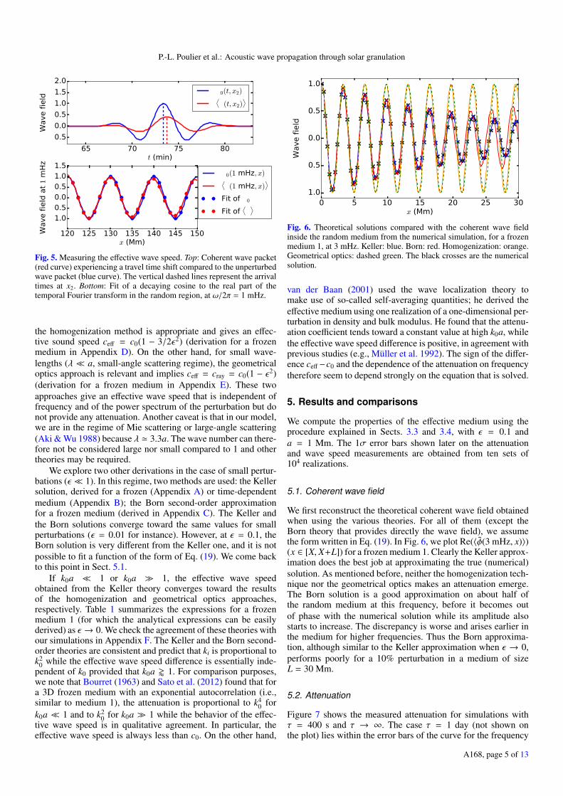
Fig. 6. Theoretical solutions compared with the coherent wave fieldinside the random medium from the numerical simulation, for a frozenmedium 1, at 3 mHz. Keller: blue. Born: red. Homogenization: orange.Geometrical optics: dashed green. The black crosses are the numericalsolution.

van der Baan (2001) used the wave localization theory tomake use of so-called self-averaging quantities; he derived theeffective medium using one realization of a one-dimensional per-turbation in density and bulk modulus. He found that the attenu-ation coefficient tends toward a constant value at high k0a, whilethe effective wave speed difference is positive, in agreement withprevious studies (e.g., Müller et al. 1992). The sign of the differ-ence ceff−c0 and the dependence of the attenuation on frequencytherefore seem to depend strongly on the equation that is solved.

5. Results and comparisons

We compute the properties of the effective medium using theprocedure explained in Sects. 3.3 and 3.4, with ε = 0.1 anda = 1 Mm. The 1σ error bars shown later on the attenuationand wave speed measurements are obtained from ten sets of104 realizations.

5.1. Coherent wave field

We first reconstruct the theoretical coherent wave field obtainedwhen using the various theories. For all of them (except theBorn theory that provides directly the wave field), we assumethe form written in Eq. (19). In Fig. 6, we plot Re(〈φ̃(3 mHz, x)〉)(x ∈ [X, X+L]) for a frozen medium 1. Clearly the Keller approx-imation does the best job at approximating the true (numerical)solution. As mentioned before, neither the homogenization tech-nique nor the geometrical optics makes an attenuation emerge.The Born solution is a good approximation on about half ofthe random medium at this frequency, before it becomes outof phase with the numerical solution while its amplitude alsostarts to increase. The discrepancy is worse and arises earlier inthe medium for higher frequencies. Thus the Born approxima-tion, although similar to the Keller approximation when ε → 0,performs poorly for a 10% perturbation in a medium of sizeL = 30 Mm.

5.2. Attenuation

Figure 7 shows the measured attenuation for simulations withτ = 400 s and τ → ∞. The case τ = 1 day (not shown onthe plot) lies within the error bars of the curve for the frequency

A168, page 5 of 13

A&A 643, A168 (2020)

Table 1. Theories used in this paper for the effective wave speed and attenuation in a frozen medium as ε → 0, and their range of validity.

Theory Validity range ki ceff

Keller 1964 ε � 1 ε2k0

(k0a +

k0a1+4(k0a)2

)c0

(1 − ε2

2

[3 − 4(k0a)2

1+4(k0a)2

])Born (2nd order) ε2(k0a)2 L

a � 1 (†) ' (‡)ε2k0

(k0a +

k0a1+4(k0a)2

)'(‡) c0

(1 − ε2

2

[3 − 4(k0a)2

1+4(k0a)2

])Homogenization k0a � 1 Not applicable ch = 〈c−2〉−1/2 ' c0

(1 − 3

2 ε2)

Geometrical optics k0a � 1, k0a � 2π La , ε � 1 (#) Not applicable cray = 〈c−1〉−1 ' c0(1 − ε2)

Notes. The Keller and the Born theories are for medium 1. (†)Approximation for k0a > 1 of Rytov et al. (1989a) who made the derivation for aGaussian autocorrelation function and single scattering. (‡)The dominant term is that of Keller for small perturbations (see for example Fig. F.1).(#)See Rytov et al. (1989b).

Fig. 7. Attenuation of the coherent wave packet vs frequency for media1 and 2, after propagation through a band of perturbed medium. The 1Dtheory from Keller is overplotted in dashed lines. 1 − σ error bars areshown.

code, which is to be expected as the typical time scales involved(the period of the wave, about 5 min, and the time it takes for itto travel through the medium, about 1 h) are much less than oneday. We superimpose the attenuation that one expects from thetime-dependent Keller theory.

The attenuation by medium 1 is an increasing function offrequency, with a value of about 1.5% of the wave number at3 mHz for τ = 400 s. The ratio ki/k0 is a linear function of fre-quency, meaning that ki is quadratic, as expected from the Kellertheory. For medium 2 however, the attenuation is not quadratic.It reaches about 0.5% of the wave number at 3 mHz, whichis smaller than the medium 1 value by a factor 3. The smallerattenuation values are caused by the lack of power toward lowwave numbers in the spectrum of the perturbation: the absenceof large scales in the perturbation means that the incoherencebetween the realizations of the wave packets occurs preferen-tially on small scales, thereby decreasing the overall broadeningof the wave packet. In medium 2, the ratio ki/k0 stabilizes above5 mHz for τ = 400 s, while it reaches a maximum at about 3 mHzfor τ → ∞. This may indicate that there is a preferred scale ofdamping of the coherent wave field.

5.3. Effective wave speed

Figure 8 shows the effective wave speed computed with for τ =400 s and τ → ∞, as well as the time-dependent Keller theory,the (frozen) spatial homogenization solution and the (frozen)geometrical optics solution. Like for the attenuation, the case

Fig. 8. Speed of the coherent wave packet vs frequency for media 1and 2, after propagation through a perturbed medium. The 1D theoryadapted from Keller (dashed lines) as well as the prediction from thehomogenization theory and the geometrical optics are shown. 1 − σerror bars are shown.

τ = 1 day (not shown) lies within the error bars of the curvefor the frequency code. The effective wave speed is less than theunperturbed sound speed c0. This is due in part to waves beingscattered back and forth, contributing to the overall transmittedsignal but at a later time than the unperturbed wave. The sec-ond reason is the delay experienced by forward-scattered waves.Indeed, in the regime of geometrical optics (λ/a � 1) wherescattering occurs essentially forward, the effective wave speed isgiven by the geometric velocity cray = 〈c−1〉−1 < c0.

The effective wave speed in medium 1 is an increasing func-tion of frequency, with a shift from c0 by about −0.7% at 3 mHzfor τ = 400 s. The Keller theory is in relative agreement for lowfrequencies ( f ≤ 2 mHz) but it predicts a constant wave speedat higher frequencies. On the other hand, the measured effectivewave speed in medium 2 clearly changes from the homogenizedvelocity ch at 1 mHz to the geometric velocity cray at 5 mHz.We note a remarkable agreement at all frequencies between thesimulations and the Keller theory for medium 2.

5.4. Variance of wave field

The mean of the perturbation is zero, therefore looking at thecoherent wave field may not be enough to directly detect mul-tiple scattering because one would only see oscillations mixedwithin the noise. In the regime of strong perturbations, thecoherent part would vanish and only the fluctuating part wouldremain, solely accessible via second order moments. One can

A168, page 6 of 13

P.-L. Poulier et al.: Acoustic wave propagation through solar granulation

for instance look at the envelope of the signal by studying thevariance of the wave field.

As shown in Fig. 9 and in the online movie, it is composedof three parts: a peak corresponding to the variance of the bal-listic wave packet, coda waves (late-arriving waves) propagatingforward, and coda waves propagating backward. The forward-propagating coda results from waves back-scattered an evennumber of times in the perturbed medium. The backward-propagating coda forms a plateau of width 2L and results fromsingle back-scattering. In geophysics, a connection has beenmade between the functional form of the coda in time domainand the complexity of the scattering medium (e.g., Sato et al.2012).

We decompose the domain in three regions (before, after andin the random medium) and integrate spatially the variance overeach of these three regions at tm = 8500 s, i.e. after the coherentwave packet went through the random medium and just after theplateau of back-scattered signal went out of it:

Ebsc =

∫ X

0Var(φ(x, tm)) dx, (25)

Eout =

∫ xmax

X+LVar(φ(x, tm)) dx, (26)

Etr =

∫ X+L

XVar(φ(x, tm)) dx. (27)

It gives us a measurement of the variance that, respectively, hasbeen back-scattered, transmitted or is still trapped in the slab atthis particular time. For medium 2, the back-scattered variancemakes up for about 50% of the total variance for τ = 400 s, and75% for τ = 1 day. The reason for these high amounts is thatthe spectrum of medium 2 peaks at small scales, therefore moreback-scattering takes place than for instance in medium 1 wherethese values become respectively 20% and 15%.

5.5. Dependence on correlation time of the medium

Calculations of an effective medium are easier to carry whenthe perturbation is frozen because one can work directly in thefrequency domain. Therefore, we study here how the effectiveparameters ki and ceff depend on the correlation time of themedium.

Figure 10 shows the relative errors in the attenuation, eki ,and in the effective wave speed difference, ec, between a givencorrelation time and the τ → ∞ case at 2, 3 and 4 mHz, formedium 2:

eki (ω, τ) =ki(ω, τ) − ki(ω,∞)

ki(ω,∞), (28)

ec(ω, τ) =

(ceff(ω, τ) − c0

c0−

ceff(ω,∞) − c0

c0

) (ceff(ω,∞) − c0

c0

)−1

=ceff(ω, τ) − ceff(ω,∞)

ceff(ω,∞) − c0· (29)

eki being generally positive, the attenuation is underestimatedby the frozen-medium approximation. Our understanding is thatsince the power of the perturbation mostly lies at high wave num-bers, the attenuation mostly comes from the small-scale incoher-ence between the realizations of the wave packets. Therefore,there must be two regimes: one at small values of τ where theattenuation increases with τ, and one at greater values of τwhere

0 50 100 150 2000.0

0.1

0.2

0.3

0.4

0.5

0.6

√ Var(φ)

Medium 1

Back-scattered Trapped Outgoing

2L

τ=400 s

τ=1 day

0 50 100 150 200x (Mm)

0.0

0.1

0.2

0.3

0.4

0.5

0.6

√ Var(φ)

Medium 2

Back-scattered Trapped Outgoing

2L

τ=400 s

τ=1 day

Fig. 9. Square root of the variance of the wave field as a function ofposition at a given time t = 8500 s. Top: medium 1. Bottom: medium 2.See the movie online.

400 s 1 h 1 dayCorrelation time τ

−0.1

0.0

0.1

0.2

0.3

0.4

0.5

e ki

2 mHz

3 mHz

4 mHz

400 s 1 h 1 dayCorrelation time τ

−0.10

−0.08

−0.06

−0.04

−0.02

0.00

0.02

e c

2 mHz

3 mHz

4 mHz

Fig. 10. Relative error on the attenuation (top) and the effective wavespeed difference (bottom) at 2, 3 and 4 mHz (medium 2). The error isbetween the quantities at τ and at τ → ∞. The dashed lines are thepredictions from the time-dependent Keller theory.

the attenuation decreases, because persisting scatterers start tocreate less small-scale incoherence, so less attenuation. The tran-sition between the two regimes corresponds to a resonance,located according to the theory at about τ = 195 s, τ = 180 sand τ = 135 s at 2, 3 and 4 mHz. On the other hand, ec beingnegative, the approximation overestimates the decrease in effec-tive wave speed, because longer-lived features are better “seen”

A168, page 7 of 13

A&A 643, A168 (2020)

400 s 1 h 1 dayCorrelation time τ

10-2

10-1

100

101

102

Relative error

ebsc

etr

eout

Fig. 11. Relative error in the variance integrated in space before, in andafter the random medium, at t = 8500 s. The error is between the quan-tities at τ and at τ = 1 day.

Table 2. Relative error at τ = 400 s for the measured quantities formedia 1 and 2.

Medium 1 Medium 2

Coherent wave eki −25% 29%ec −19% −5%

Variance ebsc 46% 31%

Notes. eki and ec are averaged over the three central frequencies. Forthe coherent wave field, the errors are computed using both the tempo-ral and the frequency codes. They are averaged over the three centralfrequencies 2, 3 and 4 mHz. On the other hand, since we study the vari-ance in time domain, the errors for this quantity are computed usingonly the temporal code.

by the wave packets. The decrease is therefore a monotonic func-tion of τ, with its asymptotic value at τ→ ∞ only determined bythe value of the ratio of the wave number over the typical size ofthe scatterer. The error is frequency-dependent and, on averageover the three central frequencies, is 29% (respectively −5%) forthe attenuation (respectively the effective wave speed difference)at τ = 400 s.

As for the variance, we assume τ = 1 day ' ∞. This isjustified as the propagation time in the random medium of length30 Mm is about 1 h � 1 day. We compute therefore

ebsc(τ) = (Ebsc(τ) − Ebsc(1 day))/Ebsc(1 day), (30)eout(τ) = (Eout(τ) − Eout(1 day))/Eout(1 day), (31)etr(τ) = (Etr(τ) − Etr(1 day))/Etr(1 day). (32)

As shown in Fig. 11, the relative errors at τ = 400 s arethen about 30%, 80% and 290% for the back-scattered, trappedand outgoing variance, respectively. Hence it appears that formedium 2, the variance is more sensitive to the correlation timethan the coherent wave field, and that the back-scattered coda isless sensitive than the rest of the variance.

The relative errors for medium 1 at τ = 400 s are presentedfor comparison purposes in Table 2. In this case, the frozen-medium approximation overestimates the attenuation. Most ofthe power is indeed located at large scales, so the attenuation ismostly caused by the large-scale incoherence between the real-izations (shifts of the wave packets), which triggers a broadeningand damping of the coherent wave packet. Therefore, the impactof scattering is larger if the scatterers persist while the wave

packets propagate through them than if the scatterers evolve intime. On the other hand, the frozen-medium approximation stilloverestimates, albeit by a larger amount, the decrease in effec-tive wave speed. The error for both quantities does not dependmuch on frequency, and is about −25% for the attenuation and−19% for the effective wave speed. For the back-scattered coda,the error increases to 46%.

6. Discussion

6.1. Accuracy of the theories

All theories predict a decrease in the effective wave speed. Theeffective wave speed and the attenuation of the coherent wavefield are best described by the Keller approximation. The Bornsecond-order solution, although consistent with the Keller solu-tion for small perturbations, performs poorly for larger ampli-tudes, therefore it may not be suited for the study of acousticwave scattering by solar granulation unless it is on small dis-tances (<30 Mm). The homogenization technique and the geo-metrical optics do not model the attenuation of the coherent wavefield. However they correctly represent the decrease in wavespeed for low and high frequencies, respectively.

6.2. Validity of the frozen-medium approximation

It is more convenient to study acoustic wave propagation in thefrequency domain, but this is easily doable only when the coef-ficients of the wave equation do not depend on time, i.e. whenone can use a snapshot of the random medium. As summarizedin Table 2, we find that for medium 2, the attenuation is underes-timated by the frozen-medium approximation by 29% at the fre-quencies of interest for the Sun. As for the effective wave speeddifference, which is an important quantity since it is directlyrelated to the helioseismic travel times, it is overestimated by5%. The greater error for ki seemingly arises from the presenceof a resonance of the function ki(τ) at a correlation time closeto that of granulation, while the effective wave speed does notexhibit such a feature. We note that the relative error in ceff − c0is similar to that of ki in medium 1, when the power of the pertur-bation is distributed at low scales. The frozen-medium approx-imation underestimates the variance of the amplitude of back-scattered coda waves by about 30%.

6.3. Detectability of coda waves

The numerical simulations show the emergence of coda waves,which are an interesting effect of multiple scattering present bothin single realizations of the wave field and in its variance, but notin the coherent wave field. Coda waves are seen trailing the bal-listic wave packet, and also as late arrival back-scattered waves(in one dimension). In helioseismology, acoustic waves are mea-sured via the two-point cross-covariance function of the solaroscillations. Therefore, in order to identify coda waves in theSun, one needs to study the statistical variance of this cross-covariance function.

Acknowledgements. We thank Aaron C. Birch for useful discussions and com-ments. PLP is a member of the International Max Planck Research School(IMPRS) for Solar System Science at the University of Göttingen. The com-putational resources were provided by the German Data Center for SDO throughgrant 50OL1701 from the German Aerospace Center (DLR).

A168, page 8 of 13

P.-L. Poulier et al.: Acoustic wave propagation through solar granulation

ReferencesAki, K., & Richards, P. G. 2002, Quantitative Seismology, 2nd edn. (University

Science Books)Aki, K., & Wu, R. S. 1988, Scattering and Attenuation of Seismic Waves, Part I

(Springer)Ball, W. H., Beeck, B., Cameron, R. H., & Gizon, L. 2016, A&A, 592,

A159Baran, O. A. 2013, Adv. Astron. Space Phys., 3, 89Bhattacharya, J., Hanasoge, S., & Antia, H. M. 2015, ApJ, 806, 246Bourret, R. C. 1963, Appl. Sci. Res. Sect. A, 12, 223Brown, T. M. 1984, Science, 226, 687Delache, P., & Fossat, E. 1988, in Seismology of the Sun and Sun-Like Stars, ed.

E. J. Rolfe, ESA SP, 286, 671Duvall, T. L., Jr, Kosovichev, A. G., & Murawski, K. 1998, ApJ, 505, L55Gizon, L., & Birch, A. C. 2004, ApJ, 614, 472Hanasoge, S. M., Gizon, L., & Bal, G. 2013, ApJ, 773, 101Houdek, G., Trampedach, R., Aarslev, M. J., & Christensen-Dalsgaard, J. 2017,

MNRAS, 464, L124Howe, M. S. 1971, J. Fluid Mech., 45, 785

Keller, J. B. 1964, Proceedings of Symposia in Applied Mathematics(Providence, R.I.: American Mathematical Society)

Legendre, G. 2003, Ph.D. Thesis, Universite paris VILynden-Bell, D., & Ostriker, J. P. 1967, MNRAS, 136, 293Müller, G., Roth, M., & Korn, M. 1992, Geophys. J. Int., 110, 29Murawski, K., & Roberts, B. 1993a, A&A, 272, 595Murawski, K., & Roberts, B. 1993b, A&A, 272, 601Papanicolaou, G. C., & Varadhan, S. R. S. 1982, Diusion with random coeffi-

cients, eds. G. Kallianpur, P. R. Krishnaiah, & J. K. Ghosh (North Holland)Rosenthal, C. S., Christensen-Dalsgaard, J., Nordlund, Å., Stein, R. F., &

Trampedach, R. 1999, A&A, 351, 689Rytov, S. M., Kravtsov, Y. A., & Tatarskii, V. I. 1989a, Priniciples of Statistical

Radiophysics, 3. Elements of Random Fields (Springer)Rytov, S. M., Kravtsov, Y. A., & Tatarskii, V. I. 1989b, Principles of

Statistical Radiophysics, 4. Wave Propagation Through Random Media(Springer)

Sato, H., Fehler, M. C., & Maeda, T. 2012, Seismic Wave Propagation andScattering in the Heterogeneous Earth, 2nd edn. (Springer)

Schou, J., & Birch, A. C. 2020, A&A, 638, A51Title, A. M., Tarbell, T. D., Topka, K. P., et al. 1989, ApJ, 336, 475van der Baan, M. 2001, Geophys. J. Int., 145, 631

A168, page 9 of 13

A&A 643, A168 (2020)

Appendix A: Keller approximation:Time-independent random medium

Starting from a time-independent random medium c(x), we cantake the Fourier transport of the wave equation:

ω2φ̃(x, ω) + ∂2x(c2(x)φ̃(x, ω)) = 0. (A.1)

The autocorrelation written in Eq. (2) can be simplified to

〈δc(x)δc(x′ + x)〉 = c20ε

2 f (x). (A.2)

For clarity, we drop the argument ω in the expression of φ̃.Keller (1964) considers an unbounded spatially random

medium and assumes statistical homogeneity, isotropy and sta-tionarity. The calculation could be generalized to the case of alocalized perturbation, however we follow the original deriva-tion. It does accurately model our problem since the amplitudeattenuation and the effective wave speed shift arise because ofthe perturbed region. Therefore only the boundary effects are nottaken into account. Keller made the first part of his derivation intime-domain, using the fact that the Green’s function for the 3Dwave equation is essentially a delta function, which simplifiesthe calculation. In 1D however, the Green’s function is related tothe Heaviside step function. We shall first derive the Keller solu-tion in frequency domain for a frozen medium, then generalizein Appendix B to the solution in time domain.

The wave equation given by Eq. (A.1) can be written as

(L̃0 + L̃1 + L̃2)φ̃ = 0, (A.3)

where

L̃0φ̃ = ω2φ̃ + c20∂

2xφ̃, (A.4)

L̃1φ̃ = 2c0∂2x

(δc(x) φ̃

), (A.5)

L̃2φ̃ = ∂2x

(δc2(x) φ̃

). (A.6)

The unperturbed equation, assuming a constant backgroundsound speed, is

L̃0φ̃0 = 0. (A.7)

The corresponding Green’s function G0, solution ofL̃0G̃0(x, x′) = δ(x − x′) where δ is the Dirac delta function, is

G̃0(x, x′) = −i

2c20k0

eik0 |x−x′ |, (A.8)

where k0 = ω/c0. Keller has shown that one can find a new waveequation for the coherent wave field under the form

(L̃0 − 〈L̃1L̃−10 L̃1〉 + 〈L̃2〉)〈φ̃〉 = 0, (A.9)

with

(〈L̃1L̃−10 L̃1〉〈φ̃〉)(x)

=

⟨c0∂

2x

(2δc(x)

∫ ∞

−∞

dx′G̃0(x, x′)c0∂2x′ [2δc(x′)〈φ̃(x′)〉]

)⟩= 4c4

0ε2∂2

x

(∫ ∞

−∞

dx′G̃0(x, x′)∂2x′ [ f (x′ − x)〈φ̃(x′)〉]

). (A.10)

We assume that the coherent wave field also satisfies a waveequation with a complex wave number k so that

〈φ̃(x′)〉 = eikx′ . (A.11)

In this case,

∂2x′ [ f (x′ − x)〈φ̃(x′)〉] = [(∂x′ + ik)2 f (x′ − x)]eikx′ . (A.12)

Therefore,

(〈L̃1L̃−10 L̃1〉〈φ̃〉)(x) = 4c4

0ε2∂2

x

(eikxI(x)

)= 4c4

0ε2((∂x + ik)2I(x)

)〈φ̃(x)〉, (A.13)

where

I(x) =

∫ ∞

−∞

dx′ G̃0(x, x′)[(∂x′ + ik)2 f (x′ − x)]eik(x′−x). (A.14)

On the other hand,

〈L̃2〉〈φ̃〉 = −c20ε

2k2〈φ̃〉. (A.15)

Using Eqs. (A.13) and (A.15) in Eq. (A.9), the perturbed waveequation for the coherent wave field is(∂2

x + k20 − 4c2

0ε2(∂x + ik)2I(x) − ε2k2

)〈φ̃(x)〉 = 0. (A.16)

We can define the complex wave number by

k2 = k20 − 4c2

0ε2(∂x + ik)2I(x) − ε2k2. (A.17)

Since the autocorrelation function of the perturbation dependshere only on the difference x′ − x, I(x) = I. In the small-perturbation approximation, one can also replace k by k0 in theright-hand term, to get finally

k2 = k20(1 + 4c2

0ε2I − ε2). (A.18)

We note that it is possible to keep k in the right-hand side, onethen has to solve a biquadratic complex equation. Here we onlyuse the approximation.

In this paper, we used in one case an exponential correlationfunction

f1(x′ − x) = f1(ζ) = ε2e−|ζ |/a, (A.19)

where ζ = x′ − x. In this case ∂ζ f1(ζ) = −sign(ζ) f1(ζ)/a and∂2ζ f1(ζ) = f1(ζ)/a2 − 2

aδ(ζ), so that

I = −i

2c20k0a

(2ik0a − (k0a)2 +

(k0a)2

2ik0a − 1

). (A.20)

Thus

k2 = k20 + ε2k2

0

(3 −

4(k0a)2

1 + 4(k0a)2

)+2iε2k2

0

(k0a +

k0a1 + 4(k0a)2

). (A.21)

This formula gives the damping Im(k) = ki of the coherent wave〈φ̃〉 and the effective wave speed ω/Re(k) = ceff of the medium.For medium 2, we evaluate the integral numerically.

A168, page 10 of 13

P.-L. Poulier et al.: Acoustic wave propagation through solar granulation

Appendix B: Keller approximation: Time-dependentrandom medium

Here, we extend the previous analysis to a time-dependent ran-dom medium c(x, t). We rewrite the problem as follows:

(L0 + L1 + L2)φ = 0, (B.1)

where

L0φ = −∂2t φ + c2

0∂2x(φ), (B.2)

L1φ = 2c0∂2x(δc(x, t)φ), (B.3)

L2φ = ∂2x(δc(x, t)2φ). (B.4)

The associated Green’s function, solution of L0G0(t, t′, x, x′) =δ(t − t′)δ(x − x′), is

G0(x, x′, t, t′) = −1

2c0Θ(c0(t − t′) − |x − x′|), (B.5)

where Θ is the Heaviside step function. With these new opera-tors, writing the wave field as

〈φ(x, t)〉 = ei(kx−ωt), (B.6)

it follows that

(〈L1L−10 L1〉〈φ〉)(x, t) = −4c4

0ε2∂2

x

" ∞

−∞

dx′dt′G0(x, x′, t, t′)

× ∂2x′ [ f (x′ − x)g(t′ − t)〈φ(t′, x′)〉] (B.7)

and

〈L2〉〈φ〉 = c20ε

2k2〈φ〉. (B.8)

The calculations are similar to those for the time-independentrandom medium. Replacing again k by k0 in the O(ε2) terms,one gets for medium 1

k2 = k20

(1 − ε2

[1 + 2c0

τ

a1

Q1

(−2 +

Q2

Q3−

Q4

Q5

)]), (B.9)

where

Q1 = 1 − iωτ, (B.10)

Q2 = (1 − ik0a)2, (B.11)

Q3 = 1 − ik0a + Q1aτc0

, (B.12)

Q4 = (1 + ik0a)2, (B.13)

Q5 = −1 − ik0a − Q1aτc0

. (B.14)

We have demonstrated here the possibility to develop a time-dependent theory given the knowledge of the power spectrum(or autocorrelation function) of the perturbation. We note thathere too, the solution for medium 2 presented in the corpus isevaluated numerically.

Appendix C: Second-order Born approximation

Another theory is the second-order Born approximation, whichwe derive here for a time-independent random medium c(x). Itis similar to the Keller theory, but one does not look for an effec-tive wave equation satisfied by the mean wave field. Instead, onewrites the mean wave field as a series up to a certain order, eachterm being proportional to a power of ε. Using the same nota-tions for the operators as in Appendix A, denoting φ̃0 the unper-turbed wave field and φ̃1 the correction such that φ̃ = φ̃0 + φ̃1, the1st-order Born approximation reads

φ̃ = φ̃0 − L̃−10 L̃1φ̃0 + O(ε2). (C.1)

Taking the average, one gets 〈φ̃〉 = φ̃0 + O(ε2). This means thatwe have to go down to the second order:

φ̃ = φ̃0 − L̃−10 L̃1φ̃0 + L̃−1

0 L̃1L̃−10 L̃1φ̃0 − L̃−1

0 L̃2φ̃0 + O(ε3) (C.2)

which, averaged, gives

〈φ̃〉 = φ̃0 + L̃−10 〈L̃1L̃−1

0 L̃1〉φ̃0 − L̃−10 〈L̃2〉φ̃0 + O(ε3). (C.3)

We can compute 〈L̃1L̃−10 L̃1〉φ̃0 and 〈L̃2〉φ̃0 easily because these

are mostly Eqs. (A.10) and (A.15) replacing 〈φ̃(x)〉 = eikx byφ̃0(x) = eik0 x. One finally needs to apply L̃−1

0 which is a con-volution by the Green’s function. In order to converge, the inte-gration requires a compact support. To model the localization ofthe perturbation between X and X + L, we introduce the windowfunction

w(x̄) = Θ(x̄ − X) − Θ(x̄ − (X + L)) (C.4)

where x̄ = (x + x′)/2, so that

〈δc(x)δc(x′)〉 = c20ε

2e−|ζ |/aw(x̄). (C.5)

The approximate solution in [X, X + L] is

〈φ̃(x)〉 ' φ̃0(x)(1 + ε2

[32

ik0a − (k0a)2 +(k0a)2

2ik0a − 1

](x − X)

),

(C.6)

which, since ε � 1, can be written (omitting a phase term) in theform 〈φ̃(x)〉 ' eik(x−X) where k has the same expression as for theKeller theory (Eq. (A.21)). To this level of approximation, theeffective k does not depend on L.

Appendix D: Spatial homogenization

In order to perform the spatial homogenization for a time-independent random medium c(x), we consider the variable

ψ = c2φ, (D.1)

which is solution of

∂2tψ

c2 − ∂2xψ = 0. (D.2)

Multiplying the equation by ∂tψ and integrating over space, thenapplying an integration by parts, we find that

∂tE = 0, (D.3)

where

E =

∫dx

(1

2c2 (∂tψ)2 + (∂xψ)2)

(D.4)

A168, page 11 of 13

A&A 643, A168 (2020)

is an expression for the energy. Since it is invariant, we are cer-tain that the homogenization expansion converges.

The medium is assumed to vary on length scales muchshorter than the wave (for solar granulation the length scale ais at least shorter than the wave length of acoustic waves). Wemoreover assume the periodicity of the medium: c(x) = c(x + a).We separate the spatial variable x into y0, a slow-varying spa-tial scale, and y1 = y0/η, a fast-varying spatial scale, whereη = k0(ω0)a � 1 (e.g., Hanasoge et al. 2013). Then

ψ = ψ(y0, y1, t) (D.5)

and

∂x = ∂y0 +1η∂y1 , (D.6)

∂2x = ∂2

y0+

2η∂y1∂y0 +

1η2 ∂

2y1. (D.7)

We also expand the solution

ψ = ψ0 + ηψ1 + η2ψ2 + O(η3), (D.8)

where ψi = ψi(y0, y1, t) = ψi(y0, y1 + a, t). We can now proceedto solving the equation order by order. Order η−2 gives

∂2y1ψ0 = 0. (D.9)

Multiplying by ψ0, integrating over y1 and using the argument ofperiodicity, one gets∫ a

0(∂y1ψ0)2dy1 = 0, (D.10)

meaning that ψ0 does not depend on y1. Order η−1 then gives

∂2y1ψ1 = 0, (D.11)

meaning that ψ1 does not depend on y1 either. Finally, at orderη0,

∂2tψ0

c2 − ∂2y0ψ0 − ∂

2y1ψ2 = 0. (D.12)

Integrating over the fast-varying coordinate y1, invokingperiodicity, one finds the following homogenized equationfor ψ:

∂2t ψ0 −

1

c−2∂2

y0ψ0 = 0, (D.13)

where c−2 = 1a

∫ a0 c−2dy1 is a spatial average. The homoge-

nization method, used here for a periodic medium, has beengeneralized to a statistically homogeneous and ergodic randommedium, by making the period tend to ∞ (e.g., Papanicolaouet al. 1982). The spatial average identifies then with the statisti-cal average. The homogenized sound speed ch of the medium

is therefore equal to 〈c−2〉−1/2. Knowing that c = c0 + δc,c−2 ' c−2

0 (1−2δc/c0 +3δc2/c20) and 〈c−2〉 ' c−2

0 (1+3ε2). Hence:

ch = 〈c−2〉−1/2 ' c0

(1 −

32ε2

). (D.14)

We note that the spatial homogenization technique does notmake an attenuation arise.

Appendix E: Ray approximation

The geometrical optics theory, or ray theory, is an infinite-frequency approximation. In practice the applicability conditionsare (Rytov et al. 1989b):

ε � 1, (E.1)k0a � 1, (E.2)

k0a � 2πLa. (E.3)

Under these conditions, the wave travel time inside the randommedium starting at x = X is computed as an integral of the slow-ness over the ray path:

t =

∫ x

Xc−1(s) ds = (x − X) c−1. (E.4)

Assuming ergodicity of the random medium, the spatial averageidentifies with the statistical average and

cray = 〈c−1〉−1. (E.5)

Appendix F: Comparing theories with numericalsimulations in the limit ε →0

Figure F.1 summarizes the accuracy of the (frozen) Keller the-ory, the Born second-order approximation, the spatial homog-enization and the ray theory in the small-perturbation regime(ε = 0.01). For each simulation, ten sets of 104 realizationswere generated to get the error bars. For such a small pertur-bation, we are in the regime of validity of the Born and Kellertheories and the results are in agreement with the numerical sim-ulations for the attenuation and the effective wave speed. Theattenuation for medium 2 resulting from the time-domain sim-ulation differs from the attenuation from the frequency-domainone, likely because of numerical diffusion. As k0a is of orderunity in our setup, we are not a priori in the regime of validity ofthe homogenization or the geometrical optic theories. However,the geometrical optics is in good agreement with the numeri-cal simulations for medium 1, despite the fact that the conditionk0a � 2π L

a is not verified in our simulations. Medium 2 exhibits,just like for ε = 0.1, a transition from the homogenization regimeat small frequencies (<1 mHz) to the geometrical optics regimeat high frequencies (>5 mHz).

A168, page 12 of 13

P.-L. Poulier et al.: Acoustic wave propagation through solar granulation

Fig. F.1. Comparison of theories with simulations for the average wave field (ε = 0.01). Top: attenuation. Bottom: effective wave speed. Thetriangles are for the simulations in frequency domain (τ→ ∞), the squares for those in time domain (τ = 1 day). The two dashed-dotted blue linesare the Born solutions for media 1 and 2, while the yellow and orange dashed lines are the Keller solutions. 1−σ error bars are shown.

A168, page 13 of 13