acoustic scattering at a hard–soft lining transition …sjoerdr/papers/jem-2007.pdfacoustic...

J Eng MathDOI 10.1007/s10665-007-9193-z

Acoustic scattering at a hard–soft lining transitionin a flow duct

Sjoerd W. Rienstra

Received: 5 January 2007 / Accepted: 27 August 2007© Springer Science+Business Media B.V. 2007

Abstract An explicit Wiener–Hopf solution is derived to describe the scattering of sound at a hard–soft wallimpedance transition at x = 0, say, in a circular duct with uniform mean flow of Mach number M . A mode, incidentfrom the upstream hard section, scatters at x = 0 into a series of reflected modes and a series of transmitted modes.Of particular interest is the role of a possible instability along the lined wall in combination with the edge singu-larity. If one of the “upstream” running modes is to be interpreted as a downstream-running instability, an extradegree of freedom in the Wiener–Hopf analysis occurs that can be resolved by application of some form of Kuttacondition at x = 0, for example a more stringent edge condition where wall streamline deflection h = O(x3/2)

at the downstream side. In general, the effect of this Kutta condition is significant, but it is particularly large forthe plane wave at low frequencies and should therefore be easily measurable. For small Helmholtz numbers, thereflection coefficient modulus |R001| tends to (1 + M)/(1 − M) without and to 1 with Kutta condition, while theend correction tends to ∞ without and to a finite value with Kutta condition. This is exactly the same behaviour asfound for reflection at a pipe exit with flow, irrespective if this is uniform or jet flow. Although the presence of theinstability in the model is hardly a question anymore since it has been confirmed numerically, a proper mathematicalcausality analysis is still not totally watertight. Therefore, the limit of a vortex sheet, separating zero flow frommean flow, approaching the wall has been explored. Indeed, this confirms that the Helmholtz unstable mode of thefree vortex sheet transforms into the suspected mode and remains unstable. As the lined-wall vortex-sheet modelpredicts unstable behaviour for which experimental evidence is at best rare and indirect, the question may be raisedif this model is indeed a consistent simplification of reality, doing justice to the double limit of small perturbationsand a thin boundary layer. Numerical time-domain methods suffer from this instability and it is very important todecide whether the instability is at least physically genuine. Experiments based on the present problem may providea handle to resolve this stubborn question.

Keywords Aircraft noise · Duct acoustics · Impedance models · Wiener–Hopf method

S. W. Rienstra (B)Department of Mathematics and Computer Science, Eindhoven University of Technology, P.O. Box 513, 5600 MB, Eindhoven,The Netherlandse-mail: [email protected]

123

S. W. Rienstra

1 James Lighthill and aero-acoustics

James Lighthill’s involvement with aero-acoustics is legendary [1,2]. As far as aero-acoustics regards the generationof sound by aerodynamic disturbances (turbulence), Lighthill defined aero-acoustics. With the publication of hismost influential first paper [3] on the subject, certainly acoustics suddenly gained a higher profile. In contrast tomodern aero-acoustics [4], sound was barely considered to be a fluid-mechanical phenomenon. The coupling ofsound with flow was restricted to advection, and nobody knew how sound was generated by unsteady flow. Inthis first paper Lighthill showed by refined mathematical analysis and brilliant scaling arguments that the far fieldintensity (averaged energy flux) of sound produced by (compact, cold, low-subsonic) turbulent eddies (the mostinefficient type of source) is proportional to U 8, where U is the typical mean flow speed. It goes without sayingthat this paper opened a new discipline and produced an enormous amount of research and insight after it [5–7],even in unexpected areas like gravity and acoustic waves brought about by turbulence in the atmosphere of the sun[8]. A very readable review is still Crighton’s [9]. The latest developments can be found in Howe [10].

Remarkably, before Lighthill’s publications most reports of measured noise data gave a U 4 variation, whereasafter it only the 8th power dependence was recognised to be correct, the 4th power being associated to other noisesources [11]. It just goes to show how practical a good theory is.

This high power of the mean flow gave the aircraft engine engineers of the 1950s a second reason to reduce thejet speed by equipping the jet engine with a turbofan and bypass duct [12]. The first one was of course the greaterfuel efficiency that is obtained by reducing the energy flux through a cross-section A (∼ ρU 3 A) by increasing Aand decreasing U such that the thrust (∼ ρU 2 A) is fixed.

The resulting turbofan revolution of increased by-pass ratios, which started in the 1960s and still continues,controlled jet noise to an extent that the interaction noise of fan and stator became dominant. This required researchon the propagation of sound in ducts and sheared mean flow. Lighthill was of course fully aware of that, as hepromoted study of this subject directly [13] and indirectly [14].

A central issue for the interpretation of duct modes is the question of their direction of propagation. If we knowfor certain that a mode decays, either because it is cut off (carrying no energy at all) or because it is damped (energyis dissipated), this question is relatively easily answered by the direction of decay. When the mode propagatesunattenuated, we have to invoke more subtle arguments based on the direction of group velocity [15] or causalarguments based on analyticity in the complex frequency, which for the easier cases of real axial wavenumberswas translated by Lighthill [16,17] into an argument1 of a slowly increasing source strength ∼ eiωt+εt . If the axialwavenumber is not real, the mode is either damped or exponentially unstable (depending on the direction we canassociate to it), and we have a more serious problem.

Inspired by these ideas of Lighthill, we will consider a problem that originates from the topic of aircraft engine-duct acoustics. It deals with sound interacting with the vortical boundary layer—in the limit of a vortex sheet—alonga lined wall and pursues the question of a possible instability.

2 Introduction

2.1 Duct modes and boundary conditions

The sound field in a lined duct with flow may be written as an infinite sum of modes if geometry, lining and meanflow are independent of the axial coordinate. Mathematically, modes form a complete basis for the representation ofthe sound field but, physically, they are each also (self-similar) solutions of the equations. Therefore, they providemuch insight into the physical behaviour of the sound propagation. Most of our knowledge of duct acoustics is basedon understanding the modes. Even for ducts with slowly varying cross-section the concept of modes is applicablethrough the WKB ansatz of negligible intermodal interaction [18,19].

1 Of course, closely related to the older argument of adding a small amount of damping by assuming the sound speed slightly complex.

123

Acoustic scattering at a hard–soft lining transition

The configuration that we will consider here is a circular duct of constant cross-section, uniform mean flow andan acoustically soft, locally reacting wall, which can be described in the frequency domain by an impedance. Thissimple but relevant model has served for years in industry to optimise the design of aircraft-engine liners [20].

A fundamental problem in the modelling of a lined wall with uniform mean flow is the limiting form of theimpedance boundary condition when the boundary layer becomes much thinner than an acoustic wavelength. Thepresently accepted Ingard–Myers boundary condition was originally proposed by Ingard [21] for a plane wall andlater generalised by Myers [22] for curved walls. It adopts the point of view of concentrating the vorticity of theboundary layer in a vortex sheet very close but not at the wall, such that the boundary condition at the wall and thecontinuity conditions across the vortex sheet can be applied without conflict. The asymptotic analysis by Eversmanand Beckemeyer [23] of the limit of a continuous profile with vanishing boundary layer, yields the same condition,with the proviso that they avoided the critical layer and assumed the mean flow velocity nowhere being equal tothe modal phase velocity. Nevertheless it is clear that the small boundary-layer thickness and the small perturbationamplitudes involve a double limit which may be non-uniform, possibly calling for nonlinear or other conditions.

The modes in lined circular ducts with uniform mean flow are rather well understood [24]. With hard walls wehave a finite number of cut-on (axially propagating) and infinitely many cut-off (axially exponentially decaying)modes. With soft walls2 this difference is slightly blurred; all modes decay exponentially but some are weaklycut-off while the others are heavily cut-off. Apart from this difference in axial direction, there is also a markeddifference in the cross-wise (radial) direction. Most modes are present throughout the duct, but some exist onlynear the wall. They decay exponentially in the radial direction away from the wall. These modes are called surfacewaves. Some exist both with and without flow, but some only with mean flow (of either type at most two percircumferential order for a hollow duct, four for an annular duct). The ones that exist only with mean flow are thuscalled hydrodynamic surface waves [24].

2.2 Instability waves

By analogy with the Helmholtz instability along an interface between two media of different velocities, the possi-bility was raised by Tester [25] that one such hydrodynamic surface wave may have the character of an instability.This means that the mode may seem to propagate in the upstream direction if the exponential decay is followed,but in reality its direction of propagation is downstream while it increases exponentially. Tester [25] verified thisconjecture by the causality argument of Briggs and Bers [26–28] (using physically reasonable frequency dependentimpedance models) and found that the suspected surface wave indeed may be an instability, at least according tothe Briggs–Bers formalism. This was confirmed analytically by Rienstra [24] for an incompressible limit of wavesalong an impedance of mass-spring-damper type, but now using the related causality criterion of Crighton andLeppington [29,30].

In order to avoid the instability problem, Quinn and Howe [31] studied the scattering of sound at a lossless liner’sleading edge (impedance zero). In this case the only neutrally unstable hydrodynamic surface waves are convectedby the mean flow. They found qualitatively the same effects as for the airfoil trailing edge [32].

Extending these ideas, Koch and Möhring [33] analysed by a generalised Wiener–Hopf solution the scatteredsound field in a 2D duct with mean flow and a finite lined section. They allowed for possible instabilities, althoughtheir (Briggs–Bers) causality analysis was incomplete because they considered only frequency independent imped-ances, which in general cannot exist. They concluded that without instability wave available, the liner’s leading-edgesingularity could be no less than rather strong (i.e., corresponding to a singular velocity field). If there is an insta-bility, this singularity can be weak, similar to the Kutta condition for a trailing edge.3 The singularity at the liner’strailing edge is more difficult to model [35,36] (the proper modelling may well be a nonlinear one and involve

2 Note that ‘soft wall’ means throughout ‘wall of finite impedance’, not ‘pressure-release wall’.3 This Kutta condition essentially results from a delicate balance between viscous effects, nonlinear inertia and acceleration, describedby a form of triple-deck theory [32,34]. It would be of interest to investigate if any consistent high-Reynolds triple deck or other structureis possible that is compatible with no instability and no Kutta condition.

123

S. W. Rienstra

essentially a finite-thickness mean flow boundary layer) and the scattering by this edge may add a certain amountof uncertainty to the results. This, however, is greatly overshadowed by the fact that the field obtained in the linedsection becomes exponentially large when the instability is included. This is in the greatest contrast with the usualexperience in industry [20].

For a part, this may be explained by the fact that a typical liner’s impedance has a dimensionless real part (resis-tance) of the order of unity or larger. For much smaller resistances, Ronneberger [37] and Aurégan et al. [38] foundfor sound waves propagating through ducts with a finite lined section considerable amplifications when mean flowis present. Both authors suggest that this phenomenon may be explained by instability waves in the lined section,thus yielding at least an indirect proof of the existence of these waves. (Note that none of these authors comparedtheir results with [33].)

It is therefore still an open question if these modes are always or only sometimes unstable, or maybe essentiallynonlinear for any reasonable acoustic amplitude because of the very high amplification rate.

On the other hand, this is not very unlike the situation for a free-stream jet. In agreement with theory, an instabilityindeed starts off the exit edge; however, further downstream the predicted Helmholtz instability is much less than isobserved, because it quickly reaches the nonlinear regime. Still the major predicted acoustic consequences due tothe excitation of the instability are very well described by linear theory [29,39–52] and it makes sense to investigatea common situation.

In the jet-exit problem we know that the instability may be excited by vortex shedding from a sharp edge. In theinviscid models we are dealing with, the vortex shedding is enforced by application of the Kutta condition [34,49].By analogy we propose here the canonical problem of a duct, consisting of a semi-infinite hard-walled section anda semi-infinite lined section, with a mean flow that runs from the hard-walled to the soft-walled parts. The linerinstability, if available, will be excited by application of some form of Kutta condition. We deliberately consider asimpler geometry than Koch and Möhring [33], in order to achieve more analytical results and to isolate the liner’sleading-edge effects from any trailing-edge effects.

We will show that in the low-Helmholtz-number limit there results a very large acoustical difference betweenpresence and absence of the instability. In similar problems for the exhaust jet it has been shown experimentally thatthe excitation of an instability is really physical and the effect on the acoustics is just as big as the theory predicts[42,44–47,52].

2.3 Causality conditions

Rather than the Briggs–Bers criterion (BB) we will use the Crighton–Leppington [29,30] causality test (CL),because BB is not applicable to Helmholtz-type instabilities. It requires the system to have a maximum temporalgrowth rate for all real wavenumbers. Such a maximum exists for free shear layers of finite thickness [53]—or moreprecisely: a maximum Strouhal number based on the shear layer thickness—and there is probably one for a finiteboundary layer along a lined wall, but this is as yet unknown. With Helmholtz instabilities along vortex sheets ofzero thickness the growth rate is not bounded since the axial wavenumber is asymptotically linearly proportionalto the frequency. It may be true that the validity of the CL test in a stricter sense has been proved mathematicallyby Jones and Morgan [54], but since this proof relies on the rather exotic concept of ultradistribution, it is far fromcertain that there exists a one-to-one correspondence in all its conclusions between the model and the modelledphysical phenomena; for example, because of the several non-uniform limits involved.

Therefore, we will use the CL test to identify the suspicious mode in question, but with reservation, and in orderto augment the credibility of the conclusion this test will be aided by a separate analysis of the behaviour of thesemodes for a configuration of the vortex sheet set at a finite distance off the wall.

2.4 Wiener–Hopf

Although the present problem might be solved for most practical engineering purposes in a satisfactory way bymode matching, this method is not useful here as it provides (in its direct form) no control of the edge singularity

123


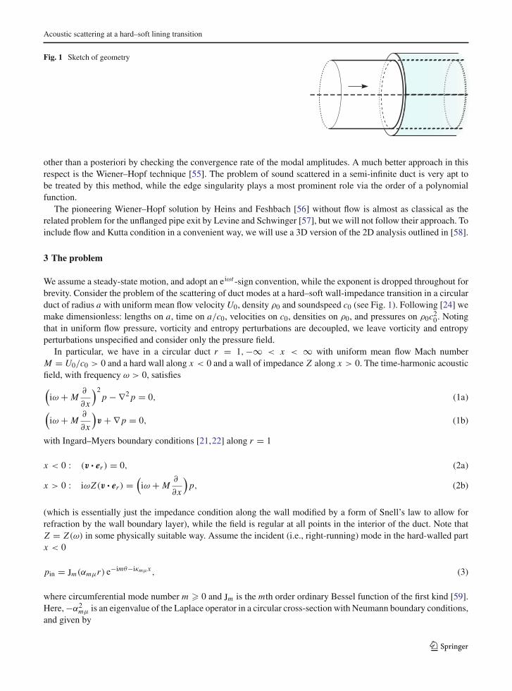
Fig. 1 Sketch of geometry

other than a posteriori by checking the convergence rate of the modal amplitudes. A much better approach in thisrespect is the Wiener–Hopf technique [55]. The problem of sound scattered in a semi-infinite duct is very apt tobe treated by this method, while the edge singularity plays a most prominent role via the order of a polynomialfunction.

The pioneering Wiener–Hopf solution by Heins and Feshbach [56] without flow is almost as classical as therelated problem for the unflanged pipe exit by Levine and Schwinger [57], but we will not follow their approach. Toinclude flow and Kutta condition in a convenient way, we will use a 3D version of the 2D analysis outlined in [58].

3 The problem

We assume a steady-state motion, and adopt an eiωt -sign convention, while the exponent is dropped throughout forbrevity. Consider the problem of the scattering of duct modes at a hard–soft wall-impedance transition in a circularduct of radius a with uniform mean flow velocity U0, density ρ0 and soundspeed c0 (see Fig. 1). Following [24] wemake dimensionless: lengths on a, time on a/c0, velocities on c0, densities on ρ0, and pressures on ρ0c2

0. Notingthat in uniform flow pressure, vorticity and entropy perturbations are decoupled, we leave vorticity and entropyperturbations unspecified and consider only the pressure field.

In particular, we have in a circular duct r = 1,−∞ < x < ∞ with uniform mean flow Mach numberM = U0/c0 > 0 and a hard wall along x < 0 and a wall of impedance Z along x > 0. The time-harmonic acousticfield, with frequency ω > 0, satisfies(

iω + M∂

∂x

)2p − ∇2 p = 0, (1a)

(iω + M

∂

∂x

)v + ∇ p = 0, (1b)

with Ingard–Myers boundary conditions [21,22] along r = 1

x < 0 : (v· er ) = 0, (2a)

x > 0 : iωZ(v· er ) =(

iω + M∂

∂x

)p, (2b)

(which is essentially just the impedance condition along the wall modified by a form of Snell’s law to allow forrefraction by the wall boundary layer), while the field is regular at all points in the interior of the duct. Note thatZ = Z(ω) in some physically suitable way. Assume the incident (i.e., right-running) mode in the hard-walled partx < 0

pin = Jm(αmµr) e−imθ−iκmµx , (3)

where circumferential mode number m � 0 and Jm is the mth order ordinary Bessel function of the first kind [59].Here, −α2

mµ is an eigenvalue of the Laplace operator in a circular cross-section with Neumann boundary conditions,and given by

123

S. W. Rienstra

α1−mmµ J′

m(αmµ) = 0, (4)

i.e., the non-trivial zeros of J′m . The quantity αmµ is usually called the radial modal wavenumber. The axial modal

wavenumber κmµ is defined through the dispersion relation

α2mµ + κ2

mµ = (ω − Mκmµ)2 (5)

such that the branch is taken with Re(κmµ) > 0 if the mode is cut-on or Im(κmµ) < 0 if the mode is cut-off. Dueto circumferential symmetry, the scattered wave will depend on θ via e−imθ only, and we will from here on assumethat p := p e−imθ where the exponent will be dropped.

After introducing the velocity potential with v = ∇φ, we can integrate (1b) to get

(iω + M

∂

∂x

)φ + p = 0. (6)

(The integration constant is not important.) So we have for the corresponding incident mode

φin = i

ω − Mκmµpin. (7)

We introduce the scattered part ψ of the potential by

φ = φin + ψ. (8)

It is convenient to reformulate the boundary condition by way of the wall streamline given by

r = 1 + Re(h(x) eiωt−imθ ), (9)

Of course, the wall streamline is not really positioned at the wall (which is not porous in the axial direction) buttaken in the limit of approaching the wall. Then the acoustic velocity between the wall streamline and the wallis uniform in the radial direction, and thus given by iωh. Furthermore, the acoustic pressure is here also uniformradially, and, being continuous across the streamline, equal to the wall pressure in the mean flow. We have then atr = 1 (note that ∂φin/∂r = 0 at r = 1)

∂ψ

∂r= 0 for x < 0, (10a)

∂ψ

∂r=

(iω + M

∂

∂x

)h for x > 0, (10b)

p = iωZh for x > 0. (10c)

We expect some singular behaviour at x = 0, but no more than what goes together with a continuous wall streamline,so h(0) = 0 and h(x+) � O(xη) for a η > 0.

123


4 The Wiener–Hopf analysis

We introduce the Fourier transforms to x

ψ̂(κ, r) =∫ ∞

−∞ψ(x, r) eiκx dx, (11a)

H+(κ) =∫ ∞

0h(x) eiκx dx, (11b)

P−(κ) =∫ 0

−∞

(iω + M

∂

∂x

)ψ(x, 1) eiκx dx, (11c)

to obtain for ψ̂ the Bessel-type equation

∂2ψ̂

∂r2 + 1

r

∂ψ̂

∂r+

[(ω − Mκ)2 − κ2 − m2

r2

]ψ̂ = 0. (12)

We introduce the reduced frequency �, Fourier wavenumber σ and radial wavenumber γ as follows

β =√

1 − M2, ω = β�, κ = �

β(σ − M),

�γ =√(ω − Mκ)2 − κ2 = �

√1 − σ 2, (13)

γ =√

1 − σ 2 where Im(γ ) � 0.

With (10a), (10b) and (11b) we arrive at the solution

ψ̂ = A(σ ) Jm(�γ r), (14a)

A(σ ) = i1 − Mσ

βγ J′m(�γ )

H+. (14b)

Since

(iω + M

∂

∂x

)ψ = pin − p, (15)

we have along the wall r = 1:

i(ω − Mκ)A Jm(�γ ) = P− +∫ ∞

0pin eiκx dx −

∫ ∞

0p eiκx dx, (16)

which reduces to

i(ω − Mκ)A Jm(�γ ) = P− + i Jm(αmµ)

κ − κmµ− iωZ H+, (17)

and

− �

β2 (1 − Mσ)2Jm(�γ )

γ J′m(�γ )

H+ + iβ�Z H+ = P− + iβ Jm(αmµ)

�(σ − σmµ), (18)

where we introduced

σmµ =√

1 − α2mµ

�2 , (19)

123

S. W. Rienstra

Fig. 2 Typical location ofsoft-wall wavenumbers τmν(indicated by ◦) andhard-wall wavenumbersσmν (indicated by ×). Notethe three soft-wall surfacewaves (Z = 0.8 − 2i,ω = 10,M = 0.5,m = 0)

−2 0 2 4 6 8 10−4

−3

−2

−1

0

1

2

3

4

such that Re(σmµ) > 0 and Im(σmµ) = 0, or Im(σmµ) < 0. This yields

P−(σ )+ iβ Jm(αmµ)

�(σ − σmµ)= −K (σ )H+(σ ), (20)

where the Wiener–Hopf kernel K is defined by

K (σ ) = �

β2 (1 − Mσ)2Jm(�γ )

γ J′m(�γ )

− iβ�Z . (21)

Note that Jm(�γ )/�γ J′m(�γ ) is a meromorphic function of �2γ 2 and therefore of σ 2. So K is a meromorphic

function of σ with isolated poles and zeros. The zeros, corresponding with the reduced axial wavenumbers in thelined part of the duct, are given by

χ(σ) = (1 − Mσ)2 Jm(�γ )− iβ3 Zγ J′m(�γ ) = 0 (22)

and denoted by σ = τmν , ν = 1, 2, . . ., for the right-running modes of the lower complex halfplane (see Fig. 2).The only4 possible candidate of a right-running mode from the upper half-plane (which then has to be an instability)will be denoted (following [24]) by σ = σH I , where the subscript refers to “hydrodynamic instability” (a possibleexample is found in the upper right corner of Fig. 2). The poles, corresponding with the reduced axial wavenumbersin the hard part of the duct, are given by

γ 1−m J′m(�γ ) = 0, (23)

denoted by σ = σmν , implicitly given by �γ = αmν , ν = 1, 2, . . . where αmν denote the non-trivial zeros ofJ′

m . For hard-walled ducts, the left and right-running reduced wavenumbers are symmetric, and so the left-runninghard-wall modes are given by σ = −σmν .

In the usual way [55] we split K into functions that are analytic in the upper and in the lower half-plane (but notea possible instability pole in the upper half-plane that really is to be counted to the lower half-plane; see Eq. (28)and below)

K (σ ) = K+(σ )K−(σ )

. (24)

4 One for each impedance surface, as follows from the surface wave arguments set out in [24] and the numerical examples te be givenbelow.

123


Following Appendix A, we introduce the auxiliary split functions N+ and N−, satisfying

K (σ ) = N+(σ )N−(σ )

(25)

and given by

log N±(σ ) = 1

2π i

∫ ∞

0

[log K (u)

u − σ− log K (−u)

u + σ

]du, (26)

where the integration contours are near but not exactly along the real axis in the way as explained in AppendicesA and B. The + sign corresponds with Im σ > 0 or Im σ = 0 & Re σ < 0, and the − sign with Im σ < 0 orIm σ = 0 & Re σ > 0. (Use for points from the opposite side the definition K N− = N+.) Following AppendixA, we obtain the following asymptotic behaviour

N±(σ ) = O(σ±1/2). (27)

When no instability pole crosses the contour, we identify

K+(σ ) = N+(σ ), K−(σ ) = N−(σ ). (28)

When an instability pole σH I crosses the contour and is to be included among the right-running modes of the lowerhalfplane, N− contains the factor (σ − σH I )

−1, so the causal split functions are

K+(σ ) = (σ − σH I )N+(σ ), K−(σ ) = (σ − σH I )N−(σ ). (29)

We continue with our analysis. We substitute the split functions in Eq. (20) to get

K−(σ )P−(σ )+ iβ Jm(αmµ)K−(σ )− K−(σmµ)

�(σ − σmµ)= −K+(σ )H+(σ )− iβ Jm(αmµ)K−(σmµ)

�(σ − σmµ). (30)

The left-hand side is a function that is analytic in the lower half-plane, while the right-hand side is analytic in theupper half-plane. So together they define an entire function E .

From the estimate h(x) = O(xη) for x ↓ 0 and η > 0, it follows [55, p. 36], that

H+(σ ) = O(σ−η−1) (|σ | → ∞,Im(σ ) > 0). (31)

This gives us the information to determine E . If there is no instability pole, then K+(σ )H+(σ ) = O(σ−η−1/2),and so E vanishes at infinity and has to vanish everywhere according to Liouville’s theorem [55]. If there is aninstability pole, we have an extra factor σ and so K+(σ )H+(σ ) = O(σ−η+1/2). This means that if η = 1/2 (nosmooth streamline at x = 0, i.e., no Kutta condition), the entire function is only bounded and equal to a constant. Ifunmodelled physical effects (nonlinearities, viscosity) require a smooth behaviour of h near x = 0, i.e., the Kuttacondition, we have to choose E = 0, as this yields η = 3/2. This is illustrated schematically in Fig. 3.

We will start with the assumption of an instability pole. As we will see, the other case will be automaticallyincluded in the formulas, and it will not be necessary to consider both cases separately.

We scale the constant E ,

E = −iβ Jm(αmµ)K−(σmµ)

�(σH I − σmµ)(1 − �) = − iβ

�Jm(αmµ)N−(σmµ)(1 − �), (32)

123

S. W. Rienstra

(a) (b) (c)

Fig. 3 Types of edge singularity. Note that in the Ingard–Myers model the perturbed wall streamline does not cross the wall. It ispositioned slightly off the wall at a distance small compared to a wavelength but large compared to any acoustic perturbation. (a) noKutta condition, no instability, (b) no Kutta condition, instability, (c) Kutta condition, instability

such that � = 0 corresponds with no excitation of the instability (no contribution from σH I ), while � = 1 corre-sponds with the full Kutta condition. Anything in between will correspond to a certain amount of instability wave,but not enough to produce a smooth solution in x = 0. It is readily verified that the assumption of no instabilitypole, i.e., K+ = N+ and E = 0, leads to exactly the same formula as with � = 0. So in the following we willidentify with condition � = 0 both the situation of no instability pole and the situation of an instability that is (forwhatever reason) not excited.

The total solution is now given by the following inverse Fourier integral, with a deformation around the poleσ = σH I if � �= 0:

p = pin + �

2π iβ2 Jm(αmµ)N−(σmµ)

∫ ∞

−∞∩ (1 − Mσ)2 Jm(�γ r)

γ J′m(�γ )N+(σ )

· · ·

×[

1

σ − σmµ− �

σ − σH I

]exp

(i�

β(M − σ)x

)dσ. (33)

(Note that the latter deformation will result in a residue contribution if x > 0.) For x < 0 we close the contouraround the lower complex half-plane, and sum over the residues of the poles in σ = −σmν , the axial wavenumbersof the left-running hard-walled modes. We obtain the field

p = pin +∞∑ν=1

Rmµν Jm(αmν) exp(

i�

β(M + σmν)x

), (34)

where

Rmµν = Jm(αmµ)N−(σmµ)(1 + Mσmν)2

β2σmν

(1 − m2

α2mν

)Jm(αmν)N+(−σmν)

[1

σmν + σmµ− �

σmν + σH I

]. (35)

In particular

R011 = 1 + M

1 − M

N−(1)N+(−1)

[1

2− �

1 + σH I

]. (36)

For the transmitted field in x > 0 we close the contour around the upper half-plane and sum over the residuesfrom σ = τmν , σmµ and (if � �= 0) σ = σH I . We note that the residue from σ = σmµ just cancels pin , while theother residues (except from σH I ) are found after employing the change of notation (cf. Eq. (22))

γ J′m(�γ )N+(σ ) = �

β2χ(σ)N−(σ ). (37)

123


Hence, we obtain

p =∞∑ν=1

Tmµν Jm(βmνr) exp(

i�

β(M − τmν)x

)

−��2

β2 Jm(αmµ)N−(σmµ)(1 − MσH I )

2

βH I J′m(βH I )N+(σH I )

Jm(βH I r) exp(

i�

β(M − σH I )x

), (38)

where βmν = �γ (τmν), βH I = �γ (σH I ), and

Tmµν = −β Jm(αmµ)N−(σmµ)(1 − Mτmν)2

χ ′(τmν)N−(τmν)

[1

τmν − σmµ− �

τmν − σH I

], (39)

while χ ′(τmν) can be further specified to be

χ ′(τmν) = −iβ2 Z Jm(βmν)

[ωτmν

(1 − m2

β2mν

− �4mν

(ωβmν Z)2

)− 2iM�mν

ωZ

], (40)

in which

�mν = ω(1 − Mτmν)

β2 . (41)

5 Causality

5.1 The CL test

To determine the direction of propagation of the modes, and thus detect any possible instability, we have availablethe following causality criteria:

– The Briggs–Bers [26–28] formalism (BB), where analyticity in the whole lower complex ω-plane is enforced bytracing the poles for fixed Re(ω), and Im(ω) running from 0 to −∞.

– The Crighton–Leppington [29,30] formalism (CL), where analyticity in the whole lower complex ω-plane isenforced by tracing the poles for fixed (but large enough) |ω|, and arg(ω) running from 0 to − 1

2π .

The CL test was originally devised for a pure Helmholtz instability without other length scales involved than theacoustic wavelength. In this case it is sufficient to rotate ω to the imaginary axis. If the situation is more complex,involving other length scales, ω may have to be increased first.

Unfortunately, the BB criterion is not applicable to Helmholtz-type instabilities as it requires the system to havea maximum temporal growth rate for all real wavenumbers. With Helmholtz instabilities the growth rate is notbounded since the axial wavenumber is asymptotically linearly proportional to the frequency. So we will use the CLprocedure, but supported by an analysis of the modes for a vortex sheet at a finite distance away from the impedancewall. This analysis will clearly show that the suspected instability is indeed the offspring of the genuine Helmholtzinstability of the free vortex sheet.

For definiteness we will model the complex, frequency-dependent impedance as a simple mass-spring-dampersystem

Z(ω) = R + iaω − ib

ω, (42)

which satisfies the fundamental requirements for Z to be physical and passive (see e.g. [60]), viz. Z is analytic andnon-zero in Im(ω) < 0, Z(ω) = Z∗(−ω) and Re(Z) > 0.

123

S. W. Rienstra

−8 −6 −4 −2 0 2 4 6 8

−30

−20

−10

0

10

20

30

−20 0 20 40 60 80

−60

−40

−20

0

20

40

60

80

−40 −20 0 20 40 60−40

−30

−20

−10

0

10

20

30

40

50

60

(a) (b) (c)

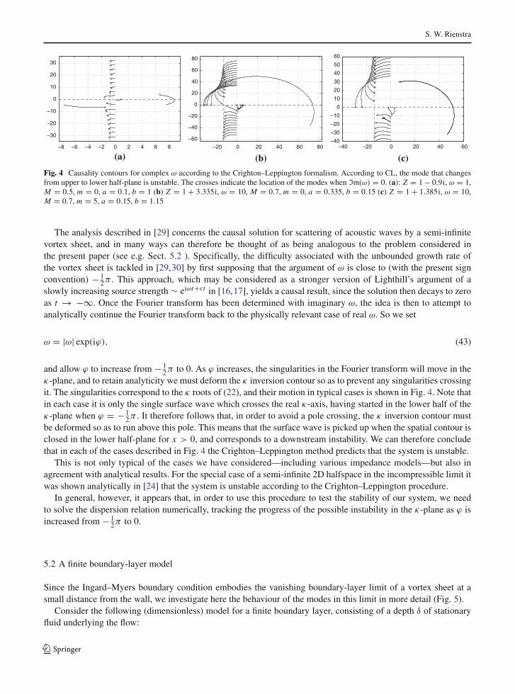
Fig. 4 Causality contours for complex ω according to the Crighton–Leppington formalism. According to CL, the mode that changesfrom upper to lower half-plane is unstable. The crosses indicate the location of the modes when Im(ω) = 0. (a): Z = 1 − 0.9i, ω = 1,M = 0.5, m = 0, a = 0.1, b = 1 (b) Z = 1 + 3.335i, ω = 10, M = 0.7, m = 0, a = 0.335, b = 0.15 (c) Z = 1 + 1.385i, ω = 10,M = 0.7, m = 5, a = 0.15, b = 1.15

The analysis described in [29] concerns the causal solution for scattering of acoustic waves by a semi-infinitevortex sheet, and in many ways can therefore be thought of as being analogous to the problem considered inthe present paper (see e.g. Sect. 5.2 ). Specifically, the difficulty associated with the unbounded growth rate ofthe vortex sheet is tackled in [29,30] by first supposing that the argument of ω is close to (with the present signconvention) − 1

2π . This approach, which may be considered as a stronger version of Lighthill’s argument of aslowly increasing source strength ∼ eiωt+εt in [16,17], yields a causal result, since the solution then decays to zeroas t → −∞. Once the Fourier transform has been determined with imaginary ω, the idea is then to attempt toanalytically continue the Fourier transform back to the physically relevant case of real ω. So we set

ω = |ω| exp(iϕ), (43)

and allow ϕ to increase from − 12π to 0. As ϕ increases, the singularities in the Fourier transform will move in the

κ-plane, and to retain analyticity we must deform the κ inversion contour so as to prevent any singularities crossingit. The singularities correspond to the κ roots of (22), and their motion in typical cases is shown in Fig. 4. Note thatin each case it is only the single surface wave which crosses the real κ-axis, having started in the lower half of theκ-plane when ϕ = − 1

2π . It therefore follows that, in order to avoid a pole crossing, the κ inversion contour mustbe deformed so as to run above this pole. This means that the surface wave is picked up when the spatial contour isclosed in the lower half-plane for x > 0, and corresponds to a downstream instability. We can therefore concludethat in each of the cases described in Fig. 4 the Crighton–Leppington method predicts that the system is unstable.

This is not only typical of the cases we have considered—including various impedance models—but also inagreement with analytical results. For the special case of a semi-infinite 2D halfspace in the incompressible limit itwas shown analytically in [24] that the system is unstable according to the Crighton–Leppington procedure.

In general, however, it appears that, in order to use this procedure to test the stability of our system, we needto solve the dispersion relation numerically, tracking the progress of the possible instability in the κ-plane as ϕ isincreased from − 1

2π to 0.

5.2 A finite boundary-layer model

Since the Ingard–Myers boundary condition embodies the vanishing boundary-layer limit of a vortex sheet at asmall distance from the wall, we investigate here the behaviour of the modes in this limit in more detail (Fig. 5).

Consider the following (dimensionless) model for a finite boundary layer, consisting of a depth δ of stationaryfluid underlying the flow:

123


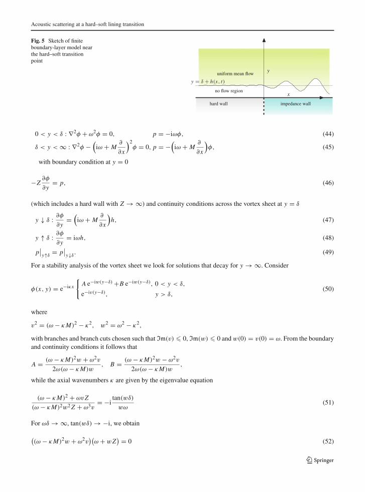
Fig. 5 Sketch of finiteboundary-layer model nearthe hard–soft transitionpoint

x

y

hard wall impedance wall

uniform mean flow

no flow region

0 < y < δ : ∇2φ + ω2φ = 0, p = −iωφ, (44)

δ < y < ∞ : ∇2φ −(

iω + M∂

∂x

)2φ = 0, p = −

(iω + M

∂

∂x

)φ, (45)

with boundary condition at y = 0

−Z∂φ

∂y= p, (46)

(which includes a hard wall with Z → ∞) and continuity conditions across the vortex sheet at y = δ

y ↓ δ : ∂φ∂y

=(

iω + M∂

∂x

)h, (47)

y ↑ δ : ∂φ∂y

= iωh, (48)

p∣∣y↑δ = p

∣∣y↓δ. (49)

For a stability analysis of the vortex sheet we look for solutions that decay for y → ∞. Consider

φ(x, y) = e−iκx

{A e−iw(y−δ)+B e−iw(y−δ), 0 < y < δ,

e−iv(y−δ), y > δ,(50)

where

v2 = (ω − κM)2 − κ2, w2 = ω2 − κ2,

with branches and branch cuts chosen such that Im(v) � 0, Im(w) � 0 andw(0) = v(0) = ω. From the boundaryand continuity conditions it follows that

A = (ω − κM)2w + ω2v

2ω(ω − κM)w, B = (ω − κM)2w − ω2v

2ω(ω − κM)w,

while the axial wavenumbers κ are given by the eigenvalue equation

(ω − κM)2 + ωvZ

(ω − κM)2w2 Z + ω3v= −i

tan(wδ)

wω(51)

For ωδ → ∞, tan(wδ) → −i, we obtain

((ω − κM)2w + ω2v

)(ω + wZ

) = 0 (52)

123

S. W. Rienstra

with two or four solutions, depending on the sign of Im(Z). If Im(Z) < 0, acoustic surface waves of the impedancewall are possible, given by [24]

κ±S = ±ω

√1 − Z−2. (53)

For the other cases, with Im(Z) � 0, no wall surface waves are possible. In either case the vortex sheet carrieshydrodynamic waves, given by Miles [61]

κ±H = ω

2M

(1 +

√1 + M2 ± i

√2 − M2 + 2

√1 + M2

). (54)

These waves are known to propagate in the direction of the mean flow (see below), so with M > 0 they propagateto the right, with κ−

H exponentially decaying and κ+H exponentially increasing. This increasing wave is known as

the compressible Kelvin–Helmholtz instability [62,63].Note that κ±

H are linearly dependent onω. The other modes κ±S are not necessarily so, but they are linearly depen-

dent for large and small ω if Z(ω) tends to infinity in these cases, which is plausible in any physical realisation.Apart from the hydrodynamic instabilities of the type of κ±

H and acoustic surface waves of the type κ±S , there are

also acoustic modes related to the duct between the wall and the vortex sheet. These are given asymptotically by

κ±n = ±

( inπ

δ− ω

πn

( iωδ

2+ 1

Z

))+ O(1/n2) (55)

for large n. For hard walls the equation reduces to

ω2v + i(ω − κM)2w tan(wδ) = 0 (56)

which yields for δ = 0 only v(κ) = 0 or κ = ±ω, which are not acceptable solutions. These are not waves thatdecay for y → ∞, so will not exist without external excitation.

For a vortex sheet close to the soft wall, i.e., ωδ → 0, we find to leading order

(ω − κM)2 + ωvZ = 0. (57)

This equation has been studied extensively elsewhere [24,58]. It describes the mode that interests us here for thelimit δ = 0, i.e., with the Ingard–Myers condition. In fact, this equation allows 0, 1, 2, 3, or 4 solutions, dependingon Z and M . These (at most) four solutions are just descendants of the four κ±

H and κ±S roots that exist for large δ

(although not necessarily continuously connected by parameter δ).The other modes that exists for any nonzero δ are given asymptotically, for small ωδ, as

κ±n = ±

( inπ

δ− ω

πnZ

)+ O(ω2δ). (58)

For impedance 1 − 2i, chosen such that all surface waves continue to exist for all δ, the typical location of thewavenumbers are given in Fig. 6. In Fig. 7 the wavenumbers of the same configurations are traced as functions ofω according to the CL test, with the impedance chosen as Z = 1 − i/ω. The other relations that were tested givevery similar behaviour. Hydrodynamic surface wave κ+

H in the first quadrant, viz. what is known to be Helmholtzunstable for δ = ∞, is clearly seen to be the mode that crosses the real axis into the fourth quadrant for any δ, andtherefore always corresponds to an instability. All others remain in the half-plane in which they started.

123


−4 −2 0 2 4 6 8 10−6

−4

−2

0

2

4

6

(a)−4 −2 0 2 4 6 8 10

−6

−4

−2

0

2

4

6

(b)−4 −2 0 2 4 6 8 10

−6

−4

−2

0

2

4

6

(c)

Fig. 6 Typical location of axial mode numbers × for varying δ, ω = 1, M = 0.5, Z = 1 − 2i. The four hydrodynamic and acousticsurface waves for δ = 0 and δ = ∞ are indicated by ◦ (δ = ∞) and � (δ = 0). (a) δ = 5 (b) δ = 0.1 (c) δ = 2 · 10−3

−4 −2 0 2 4−6

−4

−2

0

2

4

6

(a)−4 −2 0 2 4

−6

−4

−2

0

2

4

6

(b)−8 −6 −4 −2 0 2 4 6 8 10

−6

−4

−2

0

2

4

6

(c)

Fig. 7 The axial wavenumbers are tracked for complex frequency ω = |ω| eiϕ while ϕ is varied from 0 to −π/2. According to theCrighton–Leppington formalism, a wavenumber that crosses from the upper half-plane to the lower half-plane corresponds to a right-running unstable mode. This is indeed in all cases the hydrodynamic wave in the first quadrant. While Z(ω) = 1 − i/ω, all parametersare the same as in Fig. 6. (a) δ = 5 (b) δ = 0.1 (c) δ = 2 · 10−3

5.3 Summary

In summary, we can conclude that our model system is genuinely unstable for the situations described in Fig. 4where the vortex sheet is positioned at the wall, as well as for the related models of a vortex sheet at a finite distancefrom the wall where the stability properties of the system simplify to that of the well-established Kelvin–Helmholtzinstability. Indeed, this has hardly been questioned since it has recently been confirmed numerically by Chevaugeonet al. [64].

It should of course be noted that this conclusion is to some extent dependent on the functional relationshipbetween Z and ω. Different impedance models may call for further study, especially when the wall is lined by otherthan locally reacting material.

The above conclusion relates to the present model. An entirely different question is whether the physical realityis unstable. It will certainly not be unstable to the extent of streamline deflections of the order of the boundary-layerthickness; that would be prevented by the impenetrable wall. However, nothing is yet known about what mighthappen at the very early stage.

123

S. W. Rienstra

−15 −10 −5 0 5 10 15−35

−30

−25

−20

−15

−10

−5

0

5

10

15

20

25

30

35

τ−01 σ H I

τ +01

τ−02

τ +02

−2

(b)(a)−1 0 1 2 3 4

−1

−0.5

0

0.5

1

−σ01 σ01

τ−01 H I

τ +01

τ−02

σ

Fig. 8 Modal wavenumbers τ±0ν as they traverse the complex σ -plane for varying impedance Z = 1 + iλ. (a) ω = 0.1,Re(Z) =

1,m = 0,M = 0.5 (b) ω = 0.01,Re(Z) = 1,m = 0,M = 0.5

6 Low-frequency asymptotics

An interesting limit in the present context is the one for small ω. In this case the transmitted wave is very small andthe reflection coefficient R011 of the plane wave is of main interest. We have for small ω, from (21),

K (σ ) = −2(1 − Mσ)2

β2γ (σ )2+ O(ω) (ω → 0). (59)

The double zeros σ = M−1 arise from two modes, one from the upper half-plane and one from the lower half-planethat meet each other at ω = 0. These modes are of surface-wave type [24] because the radial wavenumber ispurely imaginary, but for low ω the radial decay is so slow that their confinement to the wall inside the duct ismeaningless. The mode from the upper half-plane is (in all cases considered) the instability σH I . The other oneis, in the nomenclature of [24], the right-running acoustic surface wave σS R . In the present notation it is a modefrom the set {τ0ν}, say,5 τ01 or (to avoid any ambiguity) τ+

01. For small but non-zero ω they are asymptotically givenby

σH I = M−1 + 1

2(1 + i)β2 M−2

√ωZ + · · · , (60a)

τ+01 = M−1 − 1

2(1 + i)β2 M−2

√ωZ + · · · . (60b)

This is illustrated by Fig. 8. The first two left- and right-running modes are drawn as a function of Z = 1 + iλ,where λ is varied from ∞ (hard wall) to −∞ (again hard wall). Starting as the right-running hard-wall plane waveσ01 = 1, τ+

01 becomes slightly complex, resides near M−1 when λ = 0, but returns to its starting hard-wall valuewhen λ → −∞. The second right-running mode τ+

02 (the first cut-off) disappears to real −∞. The left-runningmode τ−

01 starts as the hard-wall plane-wave mode −σ01 = −1, then moves to the right, resides near M−1 whenλ = 0 (where it apparently has changed its character and has become a right-running instability wave !) and then,instead of returning to its original hard-wall value, it disappears to real +∞. Its position has been taken over by thesecond left-running mode τ−

02.

5 There is no obvious way of sorting soft-wall modes; see Fig. 8.

123


Now we can approximate the split functions

N+(σ ) −21 − Mσ

β2(1 − σ), N−(σ ) 1 + σ

1 − Mσ, (61)

not necessarily with the same multiplicative factor as would arise from representation (A.9). For the plane-wavereflection coefficient this yields

R011 −1 + M

1 − M

(1 − 2M�

1 + M

)+ · · · (ω → 0), (62)

resulting in the remarkably different values R011 = −1 for � = 1 and R011 = −(1 + M)/(1 − M) for � = 0,irrespective of Z (although the limit Z → ∞, ω → 0 will be non-uniform). This result is exactly the same asfound for the low-frequency plane-wave reflection coefficients of a semi-infinite duct with jet or uniform mean flow[40,45–48].

The instability wave corresponding to (60a), with axial wavenumber equal to the Strouhal numberω/M , vanishesin pressure, due to the factor (1 − MσH I ), but survives in the potential or velocity. The transmission coefficient ofthe wave corresponding to (60b), with the same axial wavenumber, appears to be

T011 1

2�

(1 + M

1 − M

)1/2 + · · · . (63)

7 Results

In order to illustrate the above results we have evaluated numerically (see Appendix) the reflection coefficientsR011 of the right-running plane-wave mode (with m = 0 and µ = 1) into the left-running plane wave (also withµ = 1) as a function of frequency ω, and reflection coefficient R111 of the right-running mµ = 11-mode into itsleft-running mµ = 11-counterpart. The impedance Z = 1 − 2i and the Mach number M = 0.5 are chosen astypical of an aero-engine inlet lining, but are otherwise not special. Both modulus |R.11| and phase φ.11 are plotted,but for the lower frequencies the plane-wave phase is reformulated to an end correction δ011, i.e., the virtual pointbeyond x = 0, scaled by ω, where the wave seems to reflect with condition |p| being minimal. Since

∣∣∣e−i ω1+M x +R011 ei ω

1−M x∣∣∣2 = 1 + |R011|2 + 2|R011| cos

(2ω

1−M2 x + φ011

)

is minimal if 2ω1−M2 x + φ011 = π , so

δ011 = (1 − M2)π − φ011

2ω. (64)

In order to facilitate comparison with the low-ω analysis, the results are given, both for a small interval 0 � ω � 1and a large interval 0 � ω � 15. (The end-correction is given only for the small interval because it loses its mean-ing for higher frequencies.) The most striking result is probably the confirmation of the analytically determinedreflection coefficients 1 (� = 1, Fig. 9 left) and (1 + M)/(1 − M) (� = 0, Fig. 10 left) for ω → 0, and in additionthat the end correction tends to a finite value (Kutta condition; Fig. 9 right) and to ∞ (no Kutta condition; Fig. 10right). All this is in exact analogy with the reflection of low-frequency sound waves at the exit plane of a free jet[47] (Figs. 11, 12). Note that this behaviour is not related to ω = 0, being a resonance frequency because R111

tends to 1 at its first resonance frequency in both cases (Figs. 13 and 14).

123

S. W. Rienstra

0 0.1 0.2 0.3 0.4 0.5 0.6 0.7 0.8 0.9 10

0.25

0.5

0.75

1

1.25

1.5

1.75

2

2.25

2.5

2.75

3

ω

|R011 | at Z=1−2i, M=0.5, Γ = 0

0 0.1 0.2 0.3 0.4 0.5 0.6 0.7 0.8 0.9 10

0.25

0.5

0.75

1

1.25

1.5

1.75

2

2.25

2.5

ω

δ011

at Z=1−2i, M=0.5, Γ = 0

Fig. 9 Modulus of reflection coefficient and end correction for right-running plane wave (mµ = 01) into left-running plane wave,where the plane wave is incident from hard-walled section to lined section with impedance Z = 1 − 2i, while M = 0.5. Without Kuttacondition at x = 0

0 0.1 0.2 0.3 0.4 0.5 0.6 0.7 0.8 0.9 10

0.25

0.5

0.75

1

ω

|R011| at Z=1−2i, M=0.5, Γ = 1

0 0.1 0.2 0.3 0.4 0.5 0.6 0.7 0.8 0.9 10

0.1

0.2

0.3

0.4

0.5

ω

δ011

at Z=1−2i, M=0.5, Γ = 1

Fig. 10 Modulus of reflection coefficient and end correction for right-running plane wave (mµ = 01) into left-running plane wave,where the plane wave is incident from hard-walled section to lined section with impedance Z = 1 − 2i, while M = 0.5. With Kuttacondition at x = 0

0 1 2 3 4 5 6 7 8 9 1011121314150

0.5

1

1.5

2

2.5

3

ω

R| 011| at Z=1−2i, M=0.5, Γ = 0

0 1 2 3 4 5 6 7 8 9 1011121314150

0.5

1

ω

φ011

/π at Z=1−2i, M=0.5, Γ = 0

Fig. 11 Modulus and phase of reflection coefficient for right-running plane wave (mµ = 01) into left-running plane wave. Sameconditions as Fig. 9 but with larger frequency range

123


0 1 2 3 4 5 6 7 8 9 1011121314150

0.25

0.5

0.75

1

ω

|R 011| at Z=1−2i, M=0.5, Γ = 1

0 1 2 3 4 5 6 7 8 9 1011121314150

0.25

0.5

0.75

1

ω

φ011

/π at Z=1−2i, M=0.5, Γ = 1

Fig. 12 Modulus and phase of reflection coefficient for right-running plane wave (mµ = 01) into left-running plane wave. Sameconditions as Fig. 10 but with larger frequency range

0 1 2 3 4 5 6 7 8 9 1011121314150

0.25

0.5

0.75

1

ω

|R 111| at Z=1−2i, M=0.5, Γ = 0

0 1 2 3 4 5 6 7 8 9 1011121314150

0.25

0.5

0.75

1

ω

φ111

/π at Z=1−2i, M=0.5, Γ = 0

Fig. 13 Modulus and phase of reflection coefficient for right-running mµ = 11-mode into the same left-running mode. Otherwisesame conditions as in Fig. 11

0 1 2 3 4 5 6 7 8 9 1011121314150

0.25

0.5

0.75

1

ω

|R111| at Z=1−2i, M=0.5, Γ = 1

0 1 2 3 4 5 6 7 8 9 1011121314150

0.25

0.5

0.75

1

ω

φ111

/π at Z=1−2i, M=0.5, Γ = 1

Fig. 14 Modulus and phase of reflection coefficient for right-running mµ = 11-mode into the same left-running mode. Otherwisesame conditions as in Fig. 12

123

S. W. Rienstra

8 Conclusions

An explicit Wiener–Hopf solution has been derived to describe the scattering of duct modes at a hard–soft wallimpedance transition at x = 0 in a circular duct with uniform mean flow. A mode, incident from the hard-walledupstream region, is scattered into reflected hard-wall and transmitted soft-wall modes. A plausible edge conditionat x = 0 requires at least a continuous wall streamline r = 1 + h(x, t), no more singular than h = O(x1/2) forx ↓ 0. By analogy with a trailing-edge scattering problem, the possibility of vortex shedding from the hard–softtransition would allow us to apply the Kutta condition and require the edge condition to be no more singular thancorresponding to h = O(x3/2) for x ↓ 0.

The physical relevance of this Kutta condition is still an open question. It all depends on the direction of propaga-tion of the soft-wall modes. The Wiener–Hopf analysis shows that no Kutta condition can be applied if none of theapparently upstream running, decaying, soft-wall modes is in reality a downstream-running instability. However,causality analyses in the complex frequency domain, taking into account the frequency dependence of the imped-ance, indicate that, under certain circumstances, one soft-wall mode (per circumferential order) is to be consideredas an instability. In this case we may be able to enforce a Kutta condition and thus excite the instability.

As the growth rate of this presumed instability may be very high, it remains to be seen if this result is an artefactof the linearised model or actually representative of reality. There is thus a need for clarifying and distinguishingexperiments to be carried out. The available experiments [37,38] give indirect but convincing arguments for thepossible existence of instability waves along the liner. It is, however, not clear yet what the contributions are of theliner’s leading and trailing edge (the instability may interact with both), while the existence of the wave per se doesnot conclusively tell us what type of singularity to adopt in our model. Furthermore, the role of the boundary layerthickness (i.e., the Strouhal number based on the momentum thickness) is known to be important for the free shearlayer [53] and may be relevant here too.

We have presented results for cases with Kutta and no Kutta condition applied, and showed that the difference is,for certain choices of parameters, large enough for experimental verification. In particular, for low Helmholtz num-bers, the reflection properties become very simple and imitate the behaviour of the free jet. The pressure reflectioncoefficient for the plane wave in the low-Helmholtz-number regime is near unity with a Kutta condition, and near(1 + M)/(1 − M) with no Kutta condition applied. This low-frequency limit has the advantage that the instabilitygrowth rate reduces to zero such that nonlinear effects of the instability are postponed, while the reflection coeffi-cient becomes independent of the impedance. On the other hand, there is the practical disadvantage to be overcomethat in any experimental set-up the lined section must be very long.

Appendix A: Split functions

The complex function K (σ ) has poles and zeros in the complex plane, in particular also along the real axis. Weneed to evaluate K , written as a quotient of two functions that are respectively analytic in the upper and lowerhalf-plane, and along the real κ-axis. For reasons of causality we need to start the analysis with a complex-valuedω (with Im(ω) < 0); see Sect. 5. In that case the zeros and poles and the real κ-axis, mapped (see (13)) into theσ -plane, are typically shifted into the complex plane as indicated in Fig. 15 (the κ-axis really rotates around σ = Minstead of 0, but as long as we remain in the region of analyticity we can shift the contour to the right). A set of splitfunctions can now be constructed as follows. We want to write K (σ ) as the quotient of a function K+(σ ), whichis analytic and non-zero in the upper half-plane, and a function K−(σ ) which is analytic and non-zero in the lowerhalf-plane, while both are at most of algebraic growth at infinity:

K (σ ) = K+(σ )K−(σ )

. (A.1)

123


Fig. 15 Sketch of zeros andpoles of K (σ ) and contourof integration in thecomplex σ -plane forcomplex ω

−3 −2 −1 0 1 2 3−0.8

−0.6

−0.4

−0.2

0

0.2

0.4

0.6

0.8

C−

C+

y

ω = 10 − i

σ − plane

Construct an elongated rectangle C = C+ ∪ C− along the rotated κ-axis, which for Im(ω) < 0 makes an anglewith the real axis. Select a point y inside C. With C passing in positive orientation we have

log K (y) = 1

2π i

∮

C

log K (u)

u − ydu. (A.2)

Let the ends of C tend to ±∞ symmetrically. Since

K (σ ) ∼ �M2

β2 σ − 2M�β2 − iβ�Z (σ → ∞),

K (σ ) ∼ −�M2

β2 σ + 2M�β2 − iβ�Z (σ → −∞),

(A.3)

the contributions from the ends cancel each other to leading order, such that the total contribution tends to 0. Inparticular

limL→∞

∫ L

−L

log K (u)

u − ydu = lim

L→∞

∫ L

0

log K (u)

u − y− log K (−u)

u + ydu =

∫ ∞

0

[log K (u)


u + y

]du (A.4)

because

log K (u)


u + y= 2y

u2 log

(�M2

β2

)+ · · · (A.5)

converges. Thus we can write

log K (y) = 1

2π i

∫

C−

log K (u)

u − ydu − 1

2π i

∫

C+

log K (u)

u − ydu. (A.6)

We can identify, respectively, log(K+) and log(K−) with the first and second integral to get

K+(y) = exp[ 1

2π i

∫C−

log K (u)

u − ydu

], K−(y) = exp

[ 1

2π i

∫C+

log K (u)

u − ydu

], (A.7)

because the respective domains can be extended in an upward and downward direction without passing any sin-gularities (i.e., the integration contour). If we let Im(ω) ↑ 0, we obtain the sought split functions K± for real ω,provided we allow for any possible contour deformation if an instability pole crosses the real axis (see Sect. 5). Itis, however, more convenient not to retain this deformed contour but write

123

S. W. Rienstra

K (σ ) = N+(σ )N−(σ )

, (A.8)

where both N+ and N− are now always given by the expression

log N±(σ ) = 1

2π i

∫ ∞

0

[log K (u)


u + σ

]du. (A.9)

Wherever log K (u) is singular along the real axis, the integration contour is indented into the upper (in view of thelimit Im(ω) ↑ 0 that is taken) complex plane (see also Appendix B). The + sign corresponds with Im σ > 0 andIm σ = 0 and Re σ < 0, and the − sign with Im σ < 0 or Im σ = 0 and Re σ > 0. (Use for points from theopposite side the definition K N− = N+.) As the split functions are defined up to a multiplicative constant that isdetermined by the method of calculation, it is instructive to note that constants, like K (σ ) = c, and simple products,like K (σ ) = (σ − c+)(σ − c−), are split by (A.9) as follows.

c = c1/2

c−1/2 , (σ − c+)(σ − c−) = −i(σ − c−)−i(σ − c+)−1 (Im(c±) ≷ 0). (A.10)

When no instability pole crosses the contour, we identify

K+(σ ) = N+(σ ), K−(σ ) = N−(σ ). (A.11)

When an instability pole σH I crosses the contour, and is to be included among the right-running modes of the lowerhalf-plane, we write

K+(σ ) = (σ − σH I )N+(σ ), K−(σ ) = (σ − σH I )N−(σ ). (A.12)

If we express

K (σ ) = i�M2β−2γ (σ )L(σ ), (A.13)

then L is a well-behaved function, satisfying L(σ ) → 1 both for σ → ∞ and −∞, and can be split by the presentmethod into functions that remain bounded (see [55, p.15, Theorem C]). The factor γ (σ ) can be split by inspectioninto the quotient of (1 − σ)1/2 and (1 + σ)−1/2. As a result, we have the asymptotic estimates

N+(σ ) = O(σ 1/2), N−(σ ) = O(σ−1/2) for σ → ±∞, (A.14)

leading to corresponding behaviour for K+ and K−, depending on the included instability pole.

Appendix B: Numerical evaluation of K±

For numerical evaluation of the split functions, we need to evaluate the integral (A.9). First, we have to deal withany possible zeros and poles along the real axis. A natural way to avoid them is by deforming the contour into theupper complex plane, but taking good care to avoid any crossing of other poles or zeros (cf. [48]). A suitable choicewas found to be given by the parameterisation u = ξ(t) where

ξ(t) = t + id4t/q

3 + (t/q)4, 0 � t < ∞. (B.15)

123


−4 −3 −2 −1 0 1 2 3 4−1

−0.5

0

0.5

1

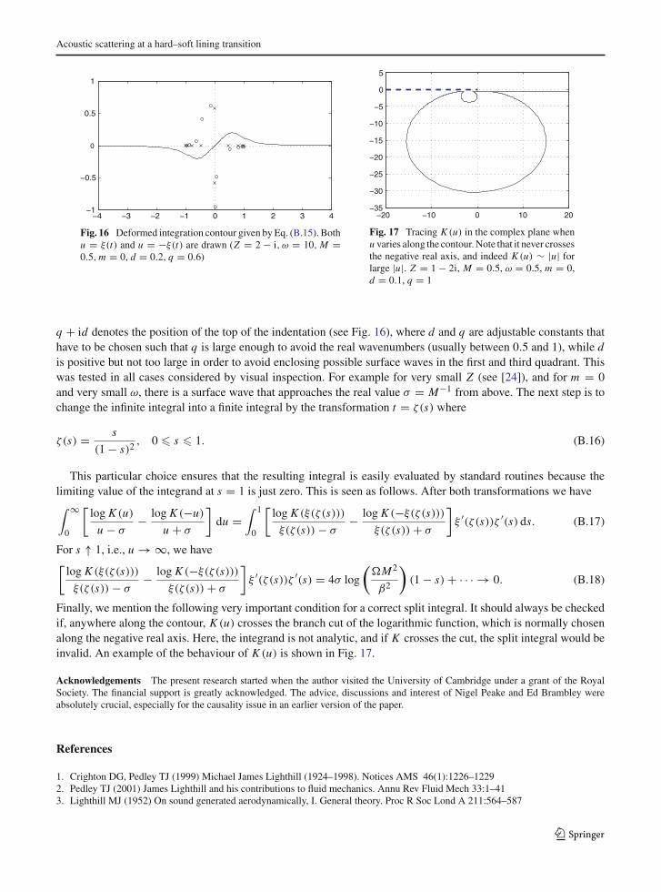
Fig. 16 Deformed integration contour given by Eq. (B.15). Bothu = ξ(t) and u = −ξ(t) are drawn (Z = 2 − i, ω = 10,M =0.5,m = 0, d = 0.2, q = 0.6)

−20 −10 0 10 20−35

−30

−25

−20

−15

−10

−5

0

5

Fig. 17 Tracing K (u) in the complex plane whenu varies along the contour. Note that it never crossesthe negative real axis, and indeed K (u) ∼ |u| forlarge |u|. Z = 1 − 2i, M = 0.5, ω = 0.5, m = 0,d = 0.1, q = 1

q + id denotes the position of the top of the indentation (see Fig. 16), where d and q are adjustable constants thathave to be chosen such that q is large enough to avoid the real wavenumbers (usually between 0.5 and 1), while dis positive but not too large in order to avoid enclosing possible surface waves in the first and third quadrant. Thiswas tested in all cases considered by visual inspection. For example for very small Z (see [24]), and for m = 0and very small ω, there is a surface wave that approaches the real value σ = M−1 from above. The next step is tochange the infinite integral into a finite integral by the transformation t = ζ(s) where

ζ(s) = s

(1 − s)2, 0 � s � 1. (B.16)

This particular choice ensures that the resulting integral is easily evaluated by standard routines because thelimiting value of the integrand at s = 1 is just zero. This is seen as follows. After both transformations we have∫ ∞

0

[log K (u)


u + σ

]du =

∫ 1

0

[log K (ξ(ζ(s)))

ξ(ζ(s))− σ− log K (−ξ(ζ(s)))

ξ(ζ(s))+ σ

]ξ ′(ζ(s))ζ ′(s) ds. (B.17)

For s ↑ 1, i.e., u → ∞, we have[

log K (ξ(ζ(s)))

ξ(ζ(s))− σ− log K (−ξ(ζ(s)))

ξ(ζ(s))+ σ

]ξ ′(ζ(s))ζ ′(s) = 4σ log

(�M2

β2

)(1 − s)+ · · · → 0. (B.18)

Finally, we mention the following very important condition for a correct split integral. It should always be checkedif, anywhere along the contour, K (u) crosses the branch cut of the logarithmic function, which is normally chosenalong the negative real axis. Here, the integrand is not analytic, and if K crosses the cut, the split integral would beinvalid. An example of the behaviour of K (u) is shown in Fig. 17.

Acknowledgements The present research started when the author visited the University of Cambridge under a grant of the RoyalSociety. The financial support is greatly acknowledged. The advice, discussions and interest of Nigel Peake and Ed Brambley wereabsolutely crucial, especially for the causality issue in an earlier version of the paper.

References

1. Crighton DG, Pedley TJ (1999) Michael James Lighthill (1924–1998). Notices AMS 46(1):1226–12292. Pedley TJ (2001) James Lighthill and his contributions to fluid mechanics. Annu Rev Fluid Mech 33:1–413. Lighthill MJ (1952) On sound generated aerodynamically, I. General theory. Proc R Soc Lond A 211:564–587

123

S. W. Rienstra

4. Crighton DG (1981) Acoustics as a branch of fluid mechanics. J Fluid Mech 106:261–2985. Lighthill MJ (1954) On sound generated aerodynamically II. Turbulence as a source of sound. Proc R Soc Lond A 222:1–326. Lighthill MJ (1962) Sound generated aerodynamically, the Bakerian Lecture 1961. Proc R Soc Lond A 267:147–1827. Lighthill MJ (1993) A general introduction to aeroacoustics and atmospheric sound. In: Hardin JC, Hussaini MY (eds) Computational

Aeroacoustics. Springer-Verlag, New York8. Stein RF (1967) Generation of acoustic and gravity waves by turbulence in an isothermal stratified atmosphere. Solar Phys 2:385–4329. Crighton DG (1975) Basic principles of aerodynamic noise generation. Prog Aerosp Sci 16:13–9610. Howe MS (2001) Vorticity and the theory of aerodynamic sound. J Eng Math 41(4):367–40011. Crighton DG (1988) Aeronautical acoustics: mathematics applied to a major industrial problem. In: McKenna J, Temam R (eds)

Proceedings of the first international conference on industrial and applied mathematics ICIAM’87. SIAM, Philadelphia, pp 75–8912. Smith MJT (1989) Aircraft noise. Cambridge University Press13. Lighthill MJ (1972) The propagation of sound through moving fluids, the fourth annual fairey lecture. J Sound Vibration 24:472–49214. Swinbanks MA (1975) The sound field generated by a source distribution in a long duct carrying sheared flow. J Sound Vibration

40(1):51–7615. Lighthill MJ (1965) Group velocity. J Inst Math Appl 1:1–2816. Lighthill MJ (1960) Studies on magneto-hydrodynamic waves and other anisotropic wave motions. Phil Trans R Soc Lond A

252:397–43017. Lighthill MJ (1978) Waves in fluids. Cambridge University Press18. Rienstra SW (1999) Sound transmission in slowly varying circular and annular lined ducts with flow. J Fluid Mech 380:279–29619. Rienstra SW (2003) Sound propagation in slowly varying lined flow ducts of arbitrary cross-section. J Fluid Mech 495:157–17320. Rademaker ER (1990) Experimental validation of a lined-duct acoustics model including flow. Presented at ASME conference on

duct acoustics, Dallas, TX, Nov. 199021. Ingard KU (1959) Influence of fluid motion past a plane boundary on sound reflection, absorption, and transmission. J Acoust Soc

Am 31(7):1035–103622. Myers MK (1980) On the acoustic boundary condition in the presence of flow. J Sound Vibration 71(3):429–43423. Eversman W, Beckemeyer RJ (1972) Transmission of sound in ducts with thin shear layers—convergence to the uniform flow

case. J Acoust Soc Am 52(1):216–22024. Rienstra SW (2003) A classification of duct modes based on surface waves. Wave Motion 37(2):119–13525. Tester BJ (1973) The propagation and attenuation of sound in ducts containing uniform or ‘Plug’ flow. J Sound Vibration 28(2):151–

20326. Bers A, Briggs RJ (1963) MIT Research Laboratory of Electronics Report No. 71 (unpublished)27. Briggs RJ (1964) Electron-stream interaction with plasmas. Monograph no. 29, MIT Press, Cambridge Massachusetts28. Bers A (1983) Space-time evolution of plasma instabilities—absolute and convective. In: Galeev AA, Sudan RN (eds) Handbook

of plasma physics: volume 1 basic plasma physics, Chapter 3.2. North Holland Publishing Company, pp 451–51729. Crighton DG, Leppington FG (1974) Radiation properties of the semi-infinite vortex sheet: the initial-value problem. J Fluid Mech

64(2):393–41430. Jones DS, Morgan JD (1972) The instability of a vortex sheet on a subsonic stream under acoustic radiation. Proc Camb Philos

Soc 72:465–48831. Quinn MC, Howe MS (1984) On the production and absorption of sound by lossless liners in the presence of mean flow. J Sound

Vibration 97(1):1–932. Rienstra SW (1981) Sound diffraction at a trailing edge. J Fluid Mech 108:443–46033. Koch W, Möhring W (1983) Eigensolutions for liners in uniform mean flow ducts. AIAA J 21:200–21334. Daniels PG (1985) On the unsteady Kutta condition. Quar J Mech Appl Math 31:49–7535. Goldstein ME (1981) The coupling between flow instabilities and incident disturbances at a leading edge. J Fluid Mech 104:217–24636. Crighton DG, Innes D (1981) Analytical models for shear-layer feed-back cycles. AIAA81-0061, AIAA Aerospace Sciences

Meeting, 19th, St. Louis, MO, 12–15 Jan. 198137. Brandes M, Ronneberger D (1995) Sound amplification in flow ducts lined with a periodic sequence of resonators. AIAA paper

95–126, 1st AIAA/CEAS Aeroacoustics Conference, Munich, Germany, 12–15 June 199538. Aurégan Y, Leroux M, Pagneux V (2005) Abnormal behavior of an acoustical liner with flow. Forum Acusticum 2005, Budapest39. Munt RM (1977) The interaction of sound with a subsonic jet issuing from a semi-infinite cylindrical pipe. J Fluid Mech 83(4):609–

64040. Munt RM (1990) Acoustic radiation properties of a jet pipe with subsonic jet flow: I. The cold jet reflection coefficient. J Sound

Vibration 142(3):413–43641. Morgan JD (1974) The interaction of sound with a semi-infinite vortex sheet. Quart J Mech Appl Math 27:465–48742. Bechert DW (1980) Sound absorption caused by vorticity shedding, demonstrated with a jet flow. J Sound Vibration 70:389–40543. Bechert DW (1988) Excitation of instability waves in free shear layers. Part 1. Theory. J Fluid Mech 186:47–6244. Howe MS (1979) Attenuation of sound in a low Mach number nozzle flow. J Fluid Mech 91:209–22945. Cargill AM (1982) Low-frequency sound radiation and generation due to the interaction of unsteady flow with a jet pipe. J Fluid

Mech 121:59–10546. Cargill AM (1982) Low frequency acoustic radiation from a jet pipe—a second order theory. J Sound Vibration 83:339–35447. Rienstra SW (1983) A small Strouhal number analysis for acoustic wave-jet flow-pipe interaction. J Sound Vibration 86:539–556

123


48. Rienstra SW (1984) Acoustic radiation from a semi-infinite annular duct in a uniform subsonic mean flow. J Sound Vibration94(2):267–288

49. Crighton DG (1985) The Kutta condition in unsteady flow. Ann Rev Fluid Mech 17:411–44550. Peters MCAM, Hirschberg A, Reijnen AJ, Wijnands APJ (1993) Damping and reflection coefficient measurements for an open

pipe at low Mach and low Helmholtz numbers. J Fluid Mech 256:499–53451. Cummings A (1983) Acoustic nonlinearities and power losses at orifices. AIAA J 22:786–79252. Allam S, Åbom M (2006) Investigation of damping and radiation using full plane wave decomposition in ducts. J Sound Vibration

292:519–53453. Michalke A (1965) On spatially growing disturbances in an inviscid shear layer. J Fluid Mech 23(3):521–54454. Jones DS, Morgan JD (1974) A linear model of a finite Helmholtz instability. Proc R Soc Lond A 344:341–36255. Noble B (1958) Methods based on the Wiener–Hopf technique. Pergamon Press, London56. Heins AE, Feshbach H (1947) The coupling of two acoustical ducts. J Math Phys 26:143–15557. Levine H, Schwinger J (1948) On the radiation of sound from an unflanged circular pipe. Phys Rev (APS) 73(4):383–40658. Rienstra SW (1986) Hydrodynamic instabilities and surface waves in a flow over an impedance wall. In: Comte-Bellot

G, Ffowcs Williams JE (eds) Proceedings IUTAM symposium ‘aero- and hydro-acoustics’ 1985 Lyon. Springer-Verlag, Heidelberg,pp 483–490

59. Abramowitz M, Stegun IA (1964) Handbook of mathematical functions. National Bureau of Standards, Dover Publications Inc.,New York

60. Rienstra SW (2006) Impedance models in time domain, including the extended Helmholtz resonator model. AIAA Paper 2006-2686,12th AIAA/CEAS Aeroacoustics Conference, 8–10 May 2006, Cambridge, MA, USA

61. Miles JW (1957) On the reflection of sound at an interface of relative motion. J Acoust Soc Am 29(2):226–22862. Kelvin L (1871) Hydrokinetic solutions and observations. Philos Mag 4(42):362–37763. von Helmholtz H (1868) On discontinuous movement of fluids. Philos Mag 4(36):337–34664. Chevaugeon N, Remacle J-F, Gallez X (2006) Discontinuous Galerkin implementation of the extended Helmholtz resonator imped-

ance model in time domain. AIAA paper 2006-2569, 12th AIAA/CEAS Aeroacoustics Conference, Cambridge, MA, 8–10 May2006

123

acoustic scattering at a hard–soft lining transition …sjoerdr/papers/jem-2007.pdfacoustic...

Documents