acoustic insights into the zooplankton dynamics of...
TRANSCRIPT

Accepted Manuscript
Acoustic insights into the zooplankton dynamics of the eastern Weddell Sea
Boris Cisewski, Volker H. Strass
PII: S0079-6611(16)30057-X
DOI: http://dx.doi.org/10.1016/j.pocean.2016.03.005
Reference: PROOCE 1700
To appear in: Progress in Oceanography
Received Date: 17 March 2015
Revised Date: 22 March 2016
Accepted Date: 23 March 2016
Please cite this article as: Cisewski, B., Strass, V.H., Acoustic insights into the zooplankton dynamics of the eastern
Weddell Sea, Progress in Oceanography (2016), doi: http://dx.doi.org/10.1016/j.pocean.2016.03.005
This is a PDF file of an unedited manuscript that has been accepted for publication. As a service to our customers
we are providing this early version of the manuscript. The manuscript will undergo copyediting, typesetting, and
review of the resulting proof before it is published in its final form. Please note that during the production process
errors may be discovered which could affect the content, and all legal disclaimers that apply to the journal pertain.

1
Acoustic insights into the zooplankton dynamics of the eastern Weddell Sea
Boris Cisewski a, b, *
, Volker H. Strass b
2nd revised version 21.03.2016
Submission for publication in
Progress in Oceanography
a Thünen-Institut für Seefischerei, Palmaille 9, 22767 Hamburg, Germany
b Alfred-Wegener-Institut Helmholtz-Zentrum für Polar und Meeresforschung, P.O. Box 120161,
27515 Bremerhaven, Germany
Corresponding author:
Tel.: (+49) 40 38905 224
Fax: (+49) 40 38905 263
Keywords: Diel vertical migration; ADCP backscatter; Diel and seasonal cycles; Eastern
Weddell Sea; Southern Ocean
2
Abstract
The success of any efforts to determine the effects of climate change on marine ecosystems
depends on understanding in the first instance the natural variations, which contemporarily
occur on the interannual and shorter time scales. Here we present results on the environmental
controls of zooplankton distribution patterns and behaviour in the eastern Weddell Sea,
Southern Ocean. Zooplankton abundance and vertical migration are derived from the mean
volume backscattering strength (MVBS) and the vertical velocity measured by moored
acoustic Doppler current profilers (ADCPs), which were deployed simultaneously at 64°S,
66.5°S and 69°S along the Greenwich Meridian from February, 2005, until March, 2008.
While these time series span a period of full three years they resolve hourly changes.
A highly persistent behavioural pattern found at all three mooring locations is the
synchronous diel vertical migration (DVM) of two distinct groups of zooplankton that migrate
between a deep residence depth during daytime and a shallow depth during nighttime. The
DVM was closely coupled to the astronomical daylight cycles. However, while the DVM was
symmetric around local noon, the annual modulation of the DVM was clearly asymmetric
around winter solstice or summer solstice, respectively, at all three mooring sites. DVM at our
observation sites persisted throughout winter, even at the highest latitude exposed to the polar
night. Since the magnitude as well as the relative rate of change of illumination is minimal at
this time, we propose that the ultimate causes of DVM separated from the light-mediated
proximal cue that coordinates it. In all three years, a marked change in the migration
behaviour occurred in late spring (late October/early November), when DVM ceased. The
complete suspension of DVM after early November is possibly caused by the combination of
two factors: (1) increased availability of food in the surface mixed layer provided by the
phytoplankton spring bloom, and (2) vanishing diurnal enhancement of the threat from
visually oriented predators when the illumination is quasi-continuous during the polar and
subpolar summer.

3
Zooplankton abundance in the water column, estimated as the mean MVBS in the depth
range 50 – 300 m, was highest end of summer and lowest mid to end winter on the average
annual cycle. However, zooplankton abundance varied several-fold between years and
between locations. Based on satellite and in situ data of chlorophyll and sea ice as well as on
hydrographic measurements, the interannual and spatial variations of zooplankton mean
abundance can be explained by differences in the magnitude of the phytoplankton spring
bloom, which develops during the seasonal sea ice retreat. Whereas the vernal ice melt
appears necessary to stimulate the blooming of phytoplankton, it is not the determinator of the
blooms magnitude, its areal extent and duration. A possible explanation for the limitation of
the phytoplankton bloom in some years is top-down control. We hypothesize that the
phytoplankton spring development can be curbed by grazing when the zooplankton had
attained high abundance by growth during the preceding summer.
1. Introduction
Zooplankton constitutes the central hub of pelagic ecosystems. It ensures the flow of
energy, harvested from the sun light and stored in organic substances by phytoplankton during
photosynthesis, from the primary producers to the higher trophic levels and thus to the marine
living resources exploitable by men. Zooplankton also plays a role in the biological pump,
hence in the uptake of CO2 from the atmosphere and the subsequent transfer of biogenic
carbon to the deep ocean (Longhurst and Garrison, 1988). To the biological pump it
contributes by two principal ways: first by release of sinking fecal pellets formed from the
ingested organic-carbon-rich food; second by migrating vertically between feeding strata near
the sun-lit surface where the phytoplankton grows and deeper resting layers, where not only
defecation but also excretion of dissolved compounds of carbon and nutrient elements occurs,
and in consequence accounts for a transport of matter from surface to depth (Steinberg et al.,

4
2000; Turner, 2014). However, zooplankton may also intercept the vertical flux of organic
carbon-rich particles by grazing on sinking phytoplankton aggregates and on fecal pellets
(Wallace et al. 2013). If the subsequent respiration occurs relocated towards the surface, an
upward flux component is created which reduces the overall downward carbon flux.
A widespread characteristic behavioural pattern of marine and fresh water zooplankton is a
diel vertical migration (DVM), in which the vertical distribution of the migrating zooplankters
changes over the 24-h day. Despite many decades of study, both the evolutionary mechanisms
behind DVM and the cues influencing it (Lampert 1989, Cohen and Forward 2009) are still
under debate. However, predator evasion is currently the most favoured hypothesis. The
most-common, so-called nocturnal vertical migration brings migrants from typically the
bathypelagic or mesopelagic zones into the epipelagic zone at night to feed, and back to depth
in daytime to decrease mortality by reducing the risk of detection by visually hunting
predators (Zaret and Suffern, 1976; Lampert, 1989).
DVM is considered a behavioural response to a combination of exogenous environmental
factors (e.g. light, gravity, temperature, salinity, oxygen, and hydrostatic pressure) and
endogenous factors (e.g. sex, age, changes in behaviour and physiology) originating from the
organism itself (Forward, 1988). Daylight is generally assumed the dominant exogenous cue
controlling DVM, because the times of migration usually correspond to the times of the rapid
light intensity changes around sunrise and sunset (see Roe, 1974; Forward, 1988; Haney,
1988; Ringelberg, 1995). The three main hypotheses for the use of light as an exogenous
stimulus for DVM are (1) preferendum or isolume hypothesis, (2) absolute intensity threshold
hypothesis and (3) the rate-of-change hypothesis (see review of Cohen and Forward 2009).
The preferendum or isolume hypothesis postulates that zooplankton follow a preferred or
optimal light level during vertical migration. The absolute intensity threshold hypothesis
states that ascent and descent by an organism are initiated when the ambient light intensity
changes below or above a specific level. Finally, the rate of change hypothesis suggests that

5
vertical movements in DVM are caused by behavioural responses to the relative rate and
direction of irradiance change from some non-fixed ambient adaption intensity.
Some authors have also addressed the effect of advection combined with DVM on the
distribution (dispersal or retention) of zooplankton whereby the organisms take advantage of
horizontal currents with vertically varying speeds and directions during their upward and
downward movements (Hardy and Gunther, 1935; Wroblewski, 1982; Manuel and O’Dor,
1997; Eiane et al., 1998; Krägefsky, 2008; Krägefsky et al., 2009).
Driven by the annual light cycle, polar environments exhibit an extreme seasonal
variability. Poleward of the latitude of the Polar Circle the sun stays below the horizon
between the autumnal and vernal equinoxes and above the horizon between the spring
equinox and the next autumn. For marine organisms, the change between continuous light
during summer and continuous darkness during winter is additionally modified by the
seasonal build-up and decay of the sea ice cover on large horizontal scale. The sea ice around
Antarctica typically covers more than 20 million km2 in winter and recedes to less than 4
million km2 during spring and summer (Zwally et al., 1983; Gloersen and Campbell, 1991). A
paradigm of marine polar biology is that the seasonal changes in ambient sun light and in the
sea ice coverage have a profound influence on the dynamics of high-latitude marine
ecosystem processes.
In the austral winter and spring, seasonal pack ice can contain algal concentrations that are
one to three orders of magnitude higher than in the water column below and provide a crucial
food source for grazers such as Antarctic krill (Euphausia superba) when the food resources
in the water column are very low (Quetin and Ross, 2009). During the austral summer, when
the sea ice edge recedes, low-salinity melt water usually stabilizes the water column and
creates a shallow mixed-layer, which facilitates primary production in a high irradiance
environment and accumulation of pelagic phytoplankton biomass, which provides the major
food supply for the zooplankton during this time of the year (Smith and Nelson, 1985). The

6
extreme variations in daylight hours, with twenty-four hours of daylight in summer, and
complete darkness at mid-winter,
relative change in
irradiance Δ e.g. Buchanan and Haney, 1980; Fortier et. al., 2001; Blachowiak-
Samolyk et. al., 2006; Cottier et al, 2006; Falk-Petersen et al., 2008; Berge et al., 2009; Benoit
et al., 2010; Rabindranath et al., 2010).
Since the pioneering work of Flagg and Smith (1989), many investigators have utilized the
echo intensity measured by acoustic Doppler current profilers (ADCPs) to examine the
temporal and spatial variability in the distribution of zooplankton biomass and diel vertical
migration for over two decades, presuming that zooplankton are the main scatterers of sound
in the typically used frequency range of 10s to 100s kHz (e.g., Heywood et al., 1991; Fischer
and Visbeck, 1993; Flagg et al., 1994; Heywood, 1996; Ashjian et al., 1998; Luo et al., 2000;
Pinot and Jansá, 2001; le - el e al., 2002; Jiang et al., 2007; Cisewski et al., 2010;
Radenac et al., 2010; Wallace et al, 2010). ADCPs can complement conventional net
sampling in an excellent way because they can be deployed in extreme environments and can
operate autonomously year-round, and thus provide sufficient spatial and temporal resolution
to yield precise estimates of timing, velocity and extent of DVM. They also have the
advantage of not being subject to avoidance problems as nets, imposed by zooplankton with
sufficient swimming power to escape moving objects (Burd and Thomson, 2012). On the
other hand, however, they have the drawback of reduced ability of identification of species
and of measuring quantitatively numbers of individuals and biomass.
Building on time series recorded over three years by self-contained ADCPs, moored at
three different locations along the Greenwich Meridian in the eastern Weddell Sea, we here
present an analysis of the meridional and interannual variability in the measured vertical
velocity and in the mean volume backscattering strength (MVBS). This study thus provides
an acoustic insight into the zooplankton vertical migration pattern and abundance changes in a
7
sub-region of the barely sampled Southern Ocean. The presented time series data enable to
track the changes that occur over three years at hourly resolution. The particular purposes of
this study are (1) to analyse and interpret the derived DVM patterns and abundance variations
for their seasonal modulation and interannual variability, (2) to scrutinize the annual
asymmetry of the diel vertical migration first described by Cisewski et al. (2010) for its
recurrence, and (3) to investigate how the environmental conditions control the distribution of
zooplankton spatially and temporally.
2. Materials and methods
2.1 Sampling programme and study area
Three expedition cruises were conducted with R. V. Polarstern during the years 2005 –
2008 in the eastern Weddell Sea, also known as the Lazarev Sea, as a contribution to the
LAKRIS-project (Lazarev Sea Krill Study) and to the International Polar Year. During these
surveys, scheduled in order to also reveal seasonal variations, a multitude of physical and
biological data were collected. The core data set analyzed in this study consists of (1)
measurements of the 3D velocity field and of backscatter strength recorded by self-contained
acoustic Doppler current profilers (SCADCPs) moored at three different locations (64°, 66.5°
and 69°S, 0°E) between February 2005 and March 2008 and (2) three interdisciplinary
surveys that were conducted in early summers 2005/2006 (S05/06), 2007/2008 (S07/08) and
winter 2006 (W06) (Table 1). These surveys cover the area between 6°W and 3°E and from
the Antarctic continental shelf at roughly 70°S to 60°S (Fig. 1). The study area is
characterized by a marked bottom topography comprising the Antarctic continental shelf,
deep abyssal plains and an isolated seamount, Maud Rise. It exhibits a complex pattern of
ocean circulation, which determines the inflow of Warm Deep Water (WDW) into the

8
Weddell Sea (Bersch et al., 1992; Gordon and Huber, 1995; Muench et al., 2001; de Steur et
al., 2007; Leach et al., 2010; Cisewski et al., 2011).
2.1.1 Hydrographic data
Between November 2005 and February 2008, 272 casts with a CTD type Sea-Bird
Electronics SBE 911plus were made during the three LAKRIS surveys, in order to map the
hydrographic fields of the study area. Of these, 106 extended to full ocean depth, while the
others were limited mostly to the upper 1,000 m of the water column. All CTD stations were
organized on a regular grid, made up of four meridional sections running between 60°S and
70°S and along 3°E, 0°E, 3°W and 6°W during the summer cruise 2005/2006. However, the
entire transect along 6°W of the planned grid had to be abandoned due to difficult ice
conditions and logistical constraints during the other two surveys in winter 2006 and summer
2007/2008. The distance between stations along the meridional sections was nominally 30
nautical miles. Water samples were collected with a Sea-Bird Carousel sampler with 24 12-l
bottles. For in situ calibration, temperatures were measured with a digital thermometer Sea-
Bird SBE35. The conductivity readings of the CTD probe were corrected by means of the
salinities of water samples, which were determined on board by a Guildline Autosal 8400A
salinometer referenced to IAPSO standard seawater. The temperature sensor was calibrated
by the manufacturer a few months prior to the cruise and afterwards to an accuracy better than
0.001 K for all surveys. Salinity derived from the CTD measurements was calibrated to a final
accuracy of better than 0.002 for all cruises by comparison to the salinity samples.
2.1.2 Vessel-mounted acoustic Doppler current profiler
During the listed surveys (Table 1) current velocities were measured continuously along
e s ip’s ra k down o 335 m dep using a vessel-mounted acoustic Doppler current
profiler (VMADCP type Ocean Surveyor; Teledyne RD Instruments USA, Poway, California,

9
153.6 kHz nominal frequency). The transducers were located 11 m below the water line and
were protected against ice floes by an acoustically transparent plastic window. The velocity
components u (eastward), v (northward) and w (upward) were averaged in 2min ensembles in
4m thick depth bins between 19 and 335 m depth. The ADCP processing was carried out by
using the CODAS3 software package developed by E. Firing and colleagues (Firing, 1991).
CATS02.01
2.1.3 Self-contained acoustic Doppler current profilers
The self-contained SCADCPs, deployed as components of oceanographic moorings, were
of type Workhorse Longranger (Teledyne RD Instruments USA, Poway, California) using a
four-beam, convex configuration with a beam angle of 20° and a frequency of 76.8 kHz. They
were moored at nominal depths between 309 and 477 m (Table 2) in upward-looking mode
and measured horizontal and vertical currents and acoustic backscatter intensity from roughly
20-480 m. The SCADCPs were employed in three different configurations depending on the
instrument’s internal data storage capacity (Table 3). While the SCADCP data of the first
deployment (early February to mid of December 2005) were analysed and presented by
Cisewski et al. (2010), we focus here on the second deployment period continuing from
December 2005 to early March 2008. For the latter, the number of depth cells was set to 80
with a bin size of 8 m. The sampling interval was set to one ping per ensemble with a ping
rate of one ping every 2 - 10 minutes (Table 3). The moorings were deployed in December
2005 during R. V. Polarstern cruise ANT-XXIII/2 and recovered during R. V. Polarstern
cruise ANT-XXIV/3 (Table 2).
10
2.1.4 Other environmental parameters
In order to examine for environmental factors that possibly exert a control on zooplankton
behavior and abundance, various variables were considered. Sunrise/sunset times and sun
angles at the mooring locations were calculated with the solar position algorithm (SPA)
introduced by Reda and Andreas (2004). The sea ice coverage and thickness were estimated
from four upward looking sonars (ULS), which were placed at about 100-150 m depth below
the sea surface at the top of the oceanographic moorings. The ULS data processing technique
is described by Strass (1998) with modifications introduced by Behrendt et al. (2012).
Because of data gaps occurring during the ULS measurements we also use Special Scanning
Microwave Imager (SSM/I)-derived sea ice concentration data, which are provided by the
National Snow and Ice Center, Boulder, Colorado. For this study we estimated the sea ice
coverage at 64°S, 66.5°S and 69°S from daily means of the available ULS data and compared
them to the nearest pixel of SSM/I data derived from the Bootstrap algorithm. Bootstrap
algorithm data (Comiso, 1999) were retrieved from NSIDC via
http://www.nsidc.org/data/nsidc-0079.html. It has to be noted that the ULS footprint is
approximately 10 m, whereas the SSM /I data is provided on a 25-km grid.
The concentration of chlorophyll a was measured at every CTD station during R. V.
Polarstern cruises ANT-XXIII/2 (Fach et al., 2007), ANT-XXIII/6 (Herrmann, 2009) and
ANT-XXIV/2 (Bathmann, 2010). These discrete in situ chlorophyll data was supplemented
by maps of the near-surface chlorophyll concentration derived from satellite remote sensing.
Satellite-sensed chlorophyll distributions were acquired using products processed and
distributed by ACRI-ST GlobColour service, supported by EU FP7 MyOcean and SA
GlobColour Projects, using ESA ENVISAT Medium Resolution Imaging Spectrometer
(MERIS) data, NASA Moderate Resolution Imaging Spectrometer (MODIS) and Sea-
Viewing Wide Field of View Sensor (SeaWiFS) data. The obtained maps indicate the
monthly mean surface concentrations within the study area for the months January, February,

11
March, November and December of the consecutive years 2005-2008. Furthermore, based on
eight-day composites, we estimated time series of the surface chlorophyll concentration at the
three mooring locations; we used a grid of 3 x 3 pixels around the mooring location and
computed the average. The GlobColour products have been derived with the GSM model and
algorithm, developed by Maritorena and Siegel (2005).
2.2 Data analysis
2.2.1 MVBS computation
The Workhorse Longranger ADCPs recorded echo intensity on a 0 to 255 automatic gain
control (AGC) count scale. The echo intensity E was converted to the mean volume
backscattering strength MVBS (dB) after the version of the sonar equation presented by
Deines (1999):
))(2))16.273((log10 2
10 rCDBWDBMx EEKRPLRTCMVBS
where C is a system constant delivered by the manufacturer (which includes transducer and
system noise characteristics and is -159.1 dB for the Workhorse Longranger), LDBM is the
10log10 (transmit pulse length/meter), PDBM is the 10log10 (transmit power/Watt), Tx is the
temperature of the transducer (°C), R is the range along the beam to scatterers (m), is the
sound absorption coefficient of seawater (dB/m) and Kc is a beam-specific scaling factor
(dB/count). We followed Brierley et al. (2006) and used beam-averaged data because the four
beams together gave a better signal-to-noise ratio than individual beams. The noise level (Er)
of all four beams was determined from the minimum values of RSSI (Received Signal
Strength Indicator) counts obtained in the remotest depth cell, when the sea surface was
outside the ADCP range. Sound velocity c and sound absorption coefficient were
considered variable with depth and time and calculated according to the UNESCO formula
introduced by Fofonoff and Millard (1983) and computed after Francois and Garrison (1982).

12
For determination of the vertical distribution of both parameters in the depth range above the
ADCP, we used CTD profiles measured at the mooring positions during deployment and
recovery. In order to construct a seasonal cycle of the sound velocity and absorption for the
full deployment period between February 2005 and March 2008, we interpolated in time all
available and occasional CTD profiles, which were conducted at the mooring sites.
2.2.2 Estimation of the vertical (migration) velocity
In order to analyse the seasonal variability of the vertical (migration) velocity, mean diel
cycles of the ADCP-derived vertical velocity were calculated for successive months. Since
the velocity uncertainty of single-ping ADCP data is too large, averaging is used to reduce the
measurement uncertainty to acceptable levels. The manufacturer indicates a single-ping
uncertainty of 146 mm s-1
for their instruments configured in longrange mode with a bin
length of 8 m. Because individual pings are independent, the statistical uncertainty of the
measurements can be reduced according the equation (TELEDYNE RD Instruments, 2013):
The statistical uncertainty of the velocity measurements reduces to standard errors of
1smm152430/146 = 1.4 mm s-1
if we average over 10.800 single-ping
ensembles, respectively, which corresponds to the theoretical precision of w averaged over a
month. According to the method first introduced by Plueddemann and Pinkel (1989) and
modified by Luo et al. (2000) and Cisewski et al. (2010), we also infer the migration velocity
for the scattering layers from e “slope” velo i y Δz/Δt of individual MVBS contours.
3. Results

13
3.1 Hydrography
For the two summer surveys, the hydrographic conditions of the upper 500 m in the study
area are illustrated by sections along the prime meridian from 60°S to 70°S (Figures 2b-d and
4b-d). The uppermost ocean surface layer consists mainly of less saline and relatively warm
Antarctic Surface Water (AASW), which caps the subsurface temperature minimum or
Winter Water (WW) layer and limits surface mixing to a mixed layer depth of 4 to 46 m in
the latitude range north of 69°S, i.e. north of the continental shelf break. For this study, the
mixed layer depth was calculated, in accordance to the definition of Cisewski et al. (2005), as
e dep a w i e in si u densi y in reased by ΔσT= 0.02 kg m-3
compared to the
uppermost valid value of a given CTD profile. The WW is the remnant of the previous winter
mixed layer stratified towards the surface by seasonal warming and freshening (Park et al.
1998). Underneath the surface layer, the Warm Deep Water (WDW; Carmack and Forster,
1975), characterized by an intermediary temperature maximum of about 1.1°C and a salinity
maximum of about 34.7, is found. In the south, the surface mixed layer of about 100–120 m
depth deepens towards the shelf break to more than 600 m near the Antarctic Slope Front
(Jacobs 1991), which separates the WW and the WDW from the colder and less saline shelf
waters near the Antarctic continent (Fahrbach et al, 2004). During austral winter 2006 (Figs.
3b-d), the mixed layer extended down to between 100 and 200 m, coincident with the base of
the WW. The WDW layer below however reveals an almost similar pattern as observed
during the foregoing summer. Considered together with the temperature time series obtained
from the ADCP thermistors, the upper 500 m temperature sections along 0°E (Figs. 2b, 3b
and 4b) reveal that the instruments were located within the WDW inflow for the whole
deployment period (February 2005 – March 2008). For a more detailed description of the
hydrography, we refer to Cisewski et al. (2011).

14
3.2 Circulation
3.2.1 Underway current observations
Figs. 2a and 4a illustrate the horizontal current vectors in the depth range 150 – 200 m for
the summer surveys 2005/2006 (S05/06) and 2007/2008 (S07/08), measured with the
VMADCP along the ship track and averaged in 5 km segments after the correction for tides.
The vectors show the highest velocity within the westward flowing Antarctic Coastal Current
(AntCC), which is confined to the Antarctic continental shelf slope and is associated with
maximum velocities of about 21-42 cm s-1
(S05/06) and 15-28 cm s-1
(S07/08). Apart from
the westward flowing AntCC, only one other persistent strong current was found in the study
area, namely a westward then southwestward circulation around the northern and
northwestern flanks of Maud Rise with maximum velocities of about 20-23 cm s-1
(S05/06)
and 13-28 cm s-1
(S07/08), respectively. In both summers, this jet is 30 to 60 km wide and
follows the 4000 and 5000 m-isobaths, which locally correspond to the deepest part of the
slope of the seamount. Above Maud Rise the water column appears rather stagnant,
evidencing the Taylor column that is caused by this topographic structure and veers the flow
around it (Ou 1991, Brandt et al. 2011). Further south, between Maud Rise and the AntCC,
weak recirculation occurs in narrow bands with maximum velocities of about 5-14 cm s-1
(S05/06) and 5-19 cm s-1
(S07/08) in varying directions. At the two westernmost transects the
velocity field is dominated by a number of mesoscale features indicative of eddies. Fig. 3a
reveals the horizontal currents in the depth range 150 – 200 for the winter survey 2006 (W06);
along the 6°W transect and at the southernmost stations of the 0°E and 3°E transects no
measurements were possible because of severe ice conditions. Unfortunately, there is also a
gap in the VMADCP da a due o a failure in e s ip’s naviga ional sys em along e 3°E
transect between 63.5°S and 64°S, which coincides with a major part of the northern gateway
for WDW. The vectors along the 3°E transect reveal the highest velocities within the AntCC

15
of about 34 cm s-1
. However, the northern jet splits off into two branches at about 64°S, 0°E.
While the northern branch flows in northwestward direction, the southern branch flows
southwestward (Cisewski et al., 2011).
3.2.2 Moored current observations
The northernmost mooring, AWI-229, was positioned at the northwestern edge of the
Maud Rise seamount at 64°S, 0°E and reveals the fluctuant current patterns of the Maud Rise
Jet (MRJ). Daily mean horizontal current speeds measured at 64°S and vertically averaged
between 100 and 200 meter depth range between 0 and 24 cm s-1
and show predominantly
northwesterly to southwesterly flow (Fig. 5a). Mooring AWI-231 was placed southwest of
Maud Rise where recirculation occurs; here the velocities range between 0 and 9 cm s-1
and
reveal northeasterly to southeasterly flow (Fig. 5b). Mooring AWI-232, which is located at
the northern flank of the AntCC that follows the Antarctic continental slope, documents a
strongly directional, northwestward flow running parallel to the depth contours (Figs. 5c and
6). Daily mean horizontal current speeds measured at 69°S, 0°E and spatially averaged
between 100 and 200 meter depth range between 0 and 13 cm s-1
and reveal a persistent
northwesterly flow (Fig. 5c).
In order to identify oscillatory signals in the ADCP time series data we computed the
power spectral density (PSD) of the horizontal and vertical velocities for each deployment
period. In our analysis, we focused on the four major semi-diurnal and diurnal tidal
constituents M2 (12.42 h, 1.93 cpd), S2 (12 h, 2.00 cpd), O1 (25.82 h, 0.93 cpd) and K1 (23.93
h, 1.00 cpd), which account for about 70-80% of the total tidal elevation in the Weddell Sea
(Robertson et al., 1988). Moreover, rapid changes of wind at the sea surface often produce
currents near the local inertial period, which ranges between 12.82 and 13.31 hours at our
mooring sites. At the two northernmost moorings (Figs. 7a and b), the power spectra of the
horizontal current speeds reveal clear maxima of energy in the vicinity of the semidiurnal

16
tides M2 and S2 and inertial periods. At the southernmost mooring (Fig. 7c), the layer-
averaged power spectra show peaks related to both the semi-diurnal and diurnal tidal
constituents. The PSDs of the vertical velocity (Figures 8a-c) have a much flatter spectral
slope – roughly one order of magnitude instead of 2.5 over the considered range of
frequencies - than the horizontal speed PSDs, and show the highest peak at a frequency of
about 1 cpd. This peak at 1 cpd, which dominates the spectrum of w, misses almost
completely, or is at least insignificant, in the spectra of u and v. This suggests that the
dominant diurnal cycle in vertical velocity is caused by something else than by tides. In the
following chapters, we will demonstrate that this clear peak reflects the diel vertical migration
of several zooplankton species. It is also interesting to note that the semidiurnal spectral peak
of w is located exactly at S2, i.e. is solar-cycle related, while the semidiurnal spectral maxima
of u and v are rather located at T and/or M2.
3.3 Sea ice coverage and chlorophyll
Color-coded mean sea ice concentration maps for the austral spring and summer months
November until March, derived from SSM/I data applying the Bootstrap algorithm, are shown
in Fig. 9. These maps reveal the seasonal decay of the sea ice cover and its interannual
variability in the study area during the sampling period. The region is characterized by a
recurring pattern of the vernal sea ice opening that begins with a polynya in vicinity of Maud
Rise, which was first identified and described by Comiso and Gordon (1987). Between 2005
and 2007 the period of sea ice cover lasts 199 (54%), 223 (61%) and 275 (75%) days per year
on average at 64°S, 66.5°S and 69°S (Table 4), respectively. The longest period of sea ice
coverage was observed at all mooring locations in 2007. Based on a comprehensive ULS data
set, Behrendt et al. (2011) showed that the mean sea ice draft along the Greenwich meridian is
relatively constant across the Weddell Gyre and only increases towards the coast. The authors
observed similar mean sea ice drafts of 0.64 and 0.65 m and periods of ice cover of 241 and

17
246 days around Maud Rise at 64°S and 66.5°S. However, towards the Antarctic coast at
69°S the mean sea ice draft is much higher with 1.7 m for a period of 320 days. We compared
the satellite-based sea ice concentrations derived from Bootstrap algorithm and ULS estimates
of sea ice in the Lazarev Sea. Our results show in agreement with Connolley (2005) that the
Bootstrap data is largely in line with the ULS data, e.g. that the end of the sea ice season
differs only by 1 to 6 days between both data sources.
Color-coded monthly mean maps of the chlorophyll a surface concentration, derived from
satellite remote sensing and shown in Fig. 10, reveal the development and decay of
phytoplankton blooms in the region during the sampling period. In the summer 2004/2005, a
distinct algae bloom developed near Maud Rise with highest Chl concentrations around the
mooring location at 66.5°S. The strongest (ChlMax > 4.5 mg m3) and largest bloom occurred in
the summer 2005/2006, extending over all mooring sites for 3 to 7 weeks after the sea ice
melt (Fig. 12). These findings were corroborated by in-situ measurements conducted during
R. V. Polarstern cruise ANT-XXIII/2. The chlorophyll a concentration, which was measured
at the end of the first mooring deployment along the prime meridian, reveals elevated
phytoplankton abundance in the upper 40 meters and a pronounced phytoplankton bloom of
up to 4.2 mg m-3
chlorophyll between 65°S and 67°S (Fig. 11d). During winter 2006, the
chlorophyll levels were below 0.1 mg m-3
along the entire transect (Fig. 11h). In the following
summer 2006/2007, the observed chlorophyll concentrations were below 0.3 mg m-3
at all
three mooring sites. Only a small bloom developed eastward of Maud Rise. In the summer
2007/2008, elevated chlorophyll levels at 64°S and 69°S indicate the development of a new
ice edge bloom (Fig. 11l).
3.4 Inference of diel vertical zooplankton migration from ADCP data
Mean 24-h cycles of the MVBS vertical distribution (with each cycle derived from 1 week
of data) for the 155 consecutive weeks are displayed in Figs. 13, 15, and 17, which exhibit a

18
variety of both distinct and diffuse bands of high backscatter. In order to illustrate and analyse
the characteristic patterns in the temporal and vertical distribution of MVBS, we have selected
twelve different weekly averaged diel patterns of the complete time series that are centred at
seasonally distinctive dates: the autumnal equinox, the winter solstice, the vernal equinox and
the summer solstice. These are shown together with the corresponding Doppler-derived
vertical velocities, w, in Figures 14, 16 and 18.
What stands out eyeing these overall 36 pairs of MVBS-w subfigures is a close match of
the dominant patterns of both parameters. The highest downward vertical velocities always
coincide with a downward sloping layer of enhanced backscatter and/or a clearance of the
water column of scatterers starting at the top, and the highest upward vertical velocities go
along with an upward sloping backscatter layer and/or a filling of the water column with
scatterers from below. The conclusion from this observation is that the streaks of high vertical
velocity are caused by the motion of assemblages of scatterers. Figures 14, 16 and 18 also
reveal a clearly diel cycle in the prominent patterns of MVBS and w. A distinct diel cycle in w
was identified before by spectral analysis (Fig. 8). What the spectra however did not reveal is
that the daily timing of upward or downward maximum vertical velocity is closely coupled to
sunrise and sunset, hence changes with season (detailed later in Section 3.5). An exception is
however the summer season, when a diel pattern is neither identifiable in the distribution of
MVBS nor in w. Because there is no known physical process that could explain these patterns
in backscatter and in w and their coupling to the daylight cycle, they are likely of biological
nature. Since both the backscatter layers and the streaks of high w appear rather as contiguous
signatures than as features, which can be related to discrete singular acoustic targets, we argue
that they result from the bulk properties and behaviour of numerous smaller animals within
the ensonified vertical bins along the ADCP acoustic beams.
A more detailed look at Figures 14a, e, i; 16a, e, i; and 18a, e, i, representing the autumnal
equinox, allows to identify a nocturnal migration pattern of at least two distinct groups of

19
migrators that is present at all three mooring sites and during all three sampled years 2005
through 2007. Generally, the one group, which we term deep migrators, is characterized in
both MVBS and Doppler vertical velocity data by quick migrations that are completed within
roughly two hours during dawn and dusk. They leave the surface layer two hours before
sunrise, descend to their daytime residence depth, and again attain the surface layer two hours
after sunset. The daytime residence depth of the deep migrators during the autumnal equinox
is revealed only in the ADCP record from 2006 at the southernmost mooring. Then and there
it was found around 470 m depth (Fig. 18e). In all other records, the daytime residence depth
of the deep migrators was below the maximum ADCP depth, even when the ADCP range
extended down to 500 m. During nighttime the deep migrators were found occupying depths
of 50 m or shallower. According to the method introduced by Cisewski et al. (2010) and in
order to determine the descend and ascend speeds of the scattering layers, the inclined MVBS
maxima associated with these migrators were fit by a hyperbolic tangent function. Mean and
maximum downward migration velocities estimated this way from the slope of the curve are -
3.0 cm s-1
and -8.0 cm s-1
. The steepest downward and upward trajectories of the deep
migrators corresponded with the highest Doppler velocities, ranging between ±2.0 cm s-1
and
±3.0 cm s-1
. The second group onsis s of “slow” migra ors descending from the surface layer
to a depth ranging between 250 m and 350 m one hour later. This group reaches its residence
depth at noon and attains the uppermost 50 meters one hour after sunset. The mean and
maximum downward/upward migration velocities estimated from the slope of the fitted
parabolic function are ±1.0 cm s-1
and ±2.0 cm s-1
, respectively.
The nocturnal migration patterns of the deep migrators are again apparent in the vertical
distribution of MVBS and vertical velocity at all three mooring sites around the winter
solstice. At 64°S, the DVM pattern is characterized by clearance of the upper water column
(e.g. Figs. 14b, j). In 2005, clearance starts three hours before sunrise and extends to more
than 300 m three hours later around noon (~11:30 GMT). Ascent occurs during the following

20
4.5 hours. At 66.5°S, the deep migrators occupy the layer between 75 and 125 m water depth
at night, yielding a strong scattering layer (Figs. 16b, f, j). They leave the surface layer three
hours before sunrise, descend quickly to a daytime residence below the ADCP depth, and
attain their nighttime residence layer again three hours after sunset. Further south at 69°S, the
MVBS distribution reveals one distinct group of deep migrators, which occupy the layer
between 170 and 200 m depth during the night (Figs 18b, f, j). Although the sun stays under
the horizon throughout the day around winter solstice, the deep migrators descend to a depth
of around 450 m starting at 9:00 GMT (Figs.18f, j). Mean and maximum slope velocities of
the corresponding scattering layer are ±2.0 cm s-1
and ±3.0 cm s-1
. After reaching their
residence depth around noon, they start to ascend soon after and attain their shallow nighttime
residence depth again at 15:00 GMT.
Nocturnal diel migration is also apparent in the MVBS and vertical velocity data at all
three mooring sites around the vernal equinox. Since the earth experiences equal hours of
daylight and darkness during autumnal and vernal equinox, the observed patterns and timing
of DVM are very similar during these periods. For example at 66.5°S, the deep migrators
reveal a similar nocturnal DVM pattern around the autumnal and the vernal equinox. In both
seasons of the years 2005 and 2006, they leave the surface layer two hours before sunrise,
descend quickly to a daytime residence below the ADCP depth, and attain the surface layer
two hours after sunset (Figs. 16a, c, e, g). DVM around the vernal equinox however is
consistently weaker in 2007 than in the two other years at all three mooring locations.
While typical nocturnal migration patterns of two distinct groups of migrators are
recognisable in both backscatter and Doppler-shift vertical velocity data observed around
autumnal equinox, winter solstice and vernal equinox, the DVM ceased between mid-
November and the summer solstice within the observed depth range at all three mooring sites
(Figs. 14d, h, l; 16d, h, l and 18d, h, l). However, no statement can be made about what
happened in the top few tens of metres. In all years, the summer distribution of MVBS reveals
21
an approximately vertically layered structure with constant depths of the scattering layers and
without indications of DVM. During summer solstice 2005/2006 at 66.5°S and 69°S (Figs
16d, 18d), highest MVBS values are found above 50m depth and lowest values below 300m.
During the other summers and at 64°S, the scatterers appear distributed more evenly over the
water column or concentrated at several deeper depth levels.
3.5 Seasonal and interannual variation of the vertical velocity
In order to analyse the seasonal and interannual variability of the migration velocity, mean
diel cycles of the Doppler-derived vertical velocity (averaged between 100 and 200 m depth)
are calculated for successive months between February 2005 and February 2008. This
analysis also considers the times of local sunrise and sunset at the different mooring positions
to examine the role of the astronomical daylight cycle. Figs. 19a-d document that the temporal
distribution of the ascent and descent velocities at 64°S peak symmetrically around noon and
reveal a clear dependence on the sun angle between January/February and October/November
of the years 2005-2007 at the northernmost mooring. In parallel with the shortening of the day
length between February and the winter solstice (June 21), the downward and upward
migration peaks shifted by around 1 h per month. The highest ascent and descent velocities
of 1.6 cm s-1
and -1.3 cm s-1
were observed in March 2005. A pronounced change of the
vertical velocity pattern occurs from mid-November 2005 to January 2006. During this
period, the synchronized diel vertical migration ceases. In February 2006 (Fig. 19b), the
nocturnal DVM resumes and lasts to November 2006. However, the monthly average
maximum ascent and descent velocities of about 1.0 cm s-1
and -0.5 cm s-1
were smaller than
those observed 2005. Between December 2006 and January 2007, no DVM patterns are
apparent. In January 2007 (Fig. 19c), DVM resumes and the highest ascent and descent
velocities of 1.4 cm s-1
and -1.4 cm s-1
, occurring between March and May, are comparable to

22
those observed in 2005. Between October 2007 and January 2008 DVM ceases again and
starts once more in February 2008 (Fig. 19d).
The migration velocities observed at 66.5°S are very similar to those observed at 64°S,
with peaks distributed symmetrically around noon, revealing a clear dependence on the sun
angle between February and October of the years 2005-2007 (Figs. 20a-d). The highest ascent
and descent velocities of 2.1 cm s-1
and -1.8 cm s-1
were observed in March/April 2005.
Between July and October, the maximum ascent and descent velocities range between 1.1 cm
s-1
and 0.6 cm s-1
, and -1.0 cm s-1
and -0.6 cm s-1
. In agreement with the observation made at
64°S, a change of the vertical velocity pattern occurs from mid-November 2005 to January
2006 when the diel vertical migration ceases. In February 2006 (Fig. 20b), the nocturnal
DVM starts again and lasts until November 2006. However, the peak ascent and descent
velocities of -0.8 cm s-1
and 0.9 cm s-1
were smaller than those observed 2005. Between
October 2006 and January 2007, no DVM patterns are apparent. In February 2007 (Fig. 20c),
DVM resumes and the highest ascent and descent velocities of 1.6 cm s-1
and -1.5 cm s-1
are
comparable to those observed the same month in 2005. Between November 2007 and January
2008 DVM ceases and resumes in February 2008 (Fig. 20d).
The location of the southernmost mooring at 69°S is exposed to extreme variations in
daylight hours, with twenty-four hours of daylight during summer (November 23 to January
19) and the sun below the horizon around mid-winter for the period May 31 to July 13. The
ascent and descent velocities are distributed symmetrically around noon and reveal a clear
dependence on the sun angle between February and April/May of the years 2005-2007 (Figs.
21a-d). However, DVM continues through the polar night until October in all three years.
With the sun under the horizon, descent occurs around 8 a.m. and ascent around 3 p.m. local
time. The maximum ascent and descent velocities in the course of the year of 1.5 cm s-1
and -
1.2 cm s-1
were observed between February and April of the years 2005-2007. During the

23
entire observation period (February 2005 to March 2008), DVM ceases between November
and January and resumes in February of the following year.
The basic DVM pattern, which evolves from synopsis of the Doppler-w measurements
taken through the whole three-year long deployment periods at all three mooring locations,
can be summarized as follows: maximum downward and upward vertical migration speeds
are distributed symmetrically around local noon; downward migration occurs during the two
hours before sunrise and upward migration during the two hours after sunset; when the sun
does not rise above the horizon during the polar night descent occurs around 8 a.m. and ascent
around 3 p.m. local time. The annual modulation of the DVM in contrast is asymmetric
relative to the summer and winter solstices; vertical migration speeds are highest during late
summer and early autumn (February until April); DVM persists throughout winter, but the
vertical speeds tend to decline between May and October; in late spring/early summer DVM
ceases and is then suspended until high summer, for the months November through January.
3.6 Seasonal and interannual variation of the integrated mean volume backscattering
strength
A different aspect of the observed asymmetry over the annual cycle is revealed by
considering temporal changes in the mean zooplankton concentration in the water column,
deduced from vertical means of normalised MVBS profiles. In order to investigate the
occurrence and the seasonality of relative changes of zooplankton backscatter, we applied a
normalisation to the acoustic data. To examine the annual cycle, daily means of MVBS,
averaged between 50 and 300 m water depth, were calculated for all mooring sites. We define
MVBSmed as the median value (in the linear domain) of all available daily averages of MVBS
values averaged between 50 and 300 m water depth. The difference between MVBS and
MVBSmed in the logarithmic domain gives the normalised MVBS value: MVBSnorm = MVBS
– MVBSmed. Generally, the time series of the normalised MVBS declined at all sites (64°S,

24
66.5°S and 69°S) during autumn towards winter and increased throughout the spring with
greatest levels observed during summer/early autumn (Figs. 22). However, the magnitude of
the observed decline/increase in MVBS50-300m was different between the locations and varied
from year to year. Fig. 22 shows that the largest autumnal decline occurred at 64°S, where the
difference between the summer maximum (2005/2006) and the winter minimum (2006)
amounted to nearly 14 dB. The three-year maximum at 64°S of about 7 dB was observed in
February 2006, followed by a 14 month lasting decreasing trend to about -5 dB in May 2007
and a re-increase during autumn towards winter to a maximum of about 4 dB in
January/February 2008. The normalised MVBS declined at 66.5 and 69°S during autumn
towards winter/early spring and re-increased throughout the spring with greatest levels
observed during summer/early autumn.
Averaging the daily normalised MVBS values obtained from the three years of
measurements yields a representation of the mean annual cycle of relative changes of
zooplankton backscatter (Fig. 23). Accordingly, the highest value at 64°S occurs in February,
at 66.5°S in December and at 69°S in April, on average over all three latitudes thus during the
season summer to early autumn. The lowest value at 64°S is found in June, at 66.5°S in
August and at 69°S in October, on average over all three latitudes thus during the season
winter to spring. Fig. 23 however also reveals that the annual averages are associated with a
large standard deviation, which is at least partly related to interannual variability. In case of
the mooring position 64°S, the differences between the three years are so large that the overall
deployment length apparently is still not long enough to obtain what can be considered a
regular mean annual cycle.
4. Discussion

25
4.1 Seasonal and interannual variability of DVM
Our 3-year long moored ADCP time series of MVBS and vertical velocity have
demonstrated diel vertical migration (DVM) to be a persistent behavioural pattern at all three
mooring sites that is closely related to the astronomical daylight cycles. The vertical migration
of zooplankton however changed in late spring/early austral summer at all three locations. In
contrast to many previous acoustic studies in other ocean regions, DVM at our observation
sites continued throughout winter, even at the highest latitude exposed to the polar night, until
late spring (late October/early November) when it ceased completely.
Examination of the temporal change of scattering layers revealed two distinct groups of
migrators at all three mooring positions: (i) deep/fast migrators: species migrating from near
the surface to below the ADCP depth (>400 m) at dawn and from their daytime residence
depth to the surface at dusk and (ii) shallow/slow migrators: species migrating from near the
surface to 350 m at dawn and to the surface at dusk (Cisewski et al., 2010). Vertical migration
speeds were estimated from the slopes of the scattering layers and from the vertical velocity
components of the ADCP, yielding average speeds of ±2.0-3.0 and ±1.0-2.0 cm s-1
and
maximum speeds of ±8.0 cm s-1
and ±3.0 cm s-1
, respectively. Thus, our analysis has shown
that the mean and maximum migration speeds estimated by the vertical component of the
ADCP velocity were generally lower than those estimated from the slopes of the different
sound scattering layers. This is consistent with other ADCP observations in the North Pacific,
Northeast Atlantic, Arabian Sea and Ligurian Sea, reported by Plueddemann and Pinkel
(1989), Heywood (1996), Luo et al. (2000) and Tarling et al. (2001), respectively. While the
migrations speeds estimated by fitting a curve to the undulating sound scattering layers
represent an estimate of the speed of the fastest coherently migrating scatterers alone, the
vertical velocities from the ADCP measure a slightly different mean speed that comes from an
intensity-weighted sum of the scatterer velocities within the ensonified volume (Plueddemann
and Pinkel, 1989). The same authors concluded that the vertical ADCP velocities can be

26
expected to underestimate the true migration rates in regions where the ratio of the intensity
of migrating scatterers to that of non-migrating scatterers is small.
While our acoustic study of the seasonal occurrence, daily timing, and pattern of diel
vertical migration, based on three years of acoustic measurements from three locations, is – to
our knowledge – unique for the Weddell Sea, some similar studies have been conducted in
other ocean regions. From the Southern Ocean too is a study based on a multitude of Drake
Passage transits by a ship equipped with a 150 kHz ADCP (Chereskin and Tarling, 2007),
which also identified DVM as a dominant source of variability, and that DVM continued
through winter. However, these Drake Passage transits did not extend to south of the polar
circle. In the central Greenland Sea, moored ADCPs were deployed for one year and
exhibited a diurnal cycle typical for vertically migrating zooplankton both in vertical velocity
and in acoustic backscatter (Fischer and Visbeck 1993). Peak ascent and descent velocities
were around ±1.5 cm s-1
. Strong seasonal variations in the DVM were evident, and the timing
as well as the migration amplitude changed with daylight as the season progressed. In summer
and during the polar night the migration became very weak and was only detectable in the
displacement of scattering layers. Benoit et al. (2010) used continuous multifrequency
echosounding validated by trammel net captures in the Arctic Ocean to analyse the vert ical
migration of polar cod in relation to the photoperiod, the thermal structure of the water
column and the vertical distribution of its main calanoid copepod prey. The DVM stopped in
May coincident with the midnight sun and increased schooling and feeding. Wallace et al.
(2010) analysed a two-year time series of acoustic backscatter and velocity data from moored
ADCPs obtained in an ice-free and a seasonally ice-covered Arctic fjord. They observed a
strong seasonal cycle in migratory behaviour in both fjords, with classic DVM apparent in
spring and autumn. However, differences in vertical migration behaviours emerged during
summertime, with no synchronous signal observed under ice-free conditions, whereas the

27
seasonally ice-covered fjord exhibited both asynchronous and weakly synchronous migration
patterns.
4.2 Environmental factors affecting DVM
4.2.1 Light
DVM during polar night
Generally assumed is that DVM at high latitudes slows down or ceases during wintertime
as food availability decreases and some zooplankton species enter diapause and so spend the
winter in the deep, dark and presumably safer interior of the ocean (Atkinson, 1998; Ashjian
et al., 2003). Our data but show that DVM persisted throughout winter even at the
southernmost mooring with only somewhat reduced vertical migration speeds. A similar
observation was made by Berge et al. (2009), who presented acoustic data from two coastal
locations in Svalbard (Kongsfjorden and Rijpfjorden at 79°N and 80°N, respectively) that
indicate continuation of synchronized DVM of zooplankton throughout Arctic winter, in both
open and ice-covered waters. The authors argue that even during the polar night DVM is
regulated by diel variations in solar and lunar illuminations, which are at intensities far below
the threshold of human perception. The observed DVM signal was greater under ice-free
conditions than under ice-covered conditions, possibly explicable through attenuation of light
by the sea-ice cover that weakens the intensity of ΔI/I in the under-ice water column.
Our data challenge the view that daylight exerts a strong exogenous cue when the sun
stays under the horizon throughout the day around winter solstice and the surface is covered
by sea ice. Our MVBS records reveal one distinct group of deep migrators at 69°S, which
occupy the layer between 170 and 200 m depth during the night and descend to below 450 m
during the day, thus a DVM between much deeper and hence darker layers than the mere top

28
100 m investigated by Berge et al. (2009). The main difference between winter and the other
seasons at the polar latitude in our observations is a deeper night-time sojourn level, 170 –
200 m in winter instead of 100 m or shallower from spring through autumn. This observation
suggests that the deep migrators in winter are more attracted by a pelagic food source than by
a food source that is associated with the sea ice. A possible explanation for this behavioural
change is a gradual move from herbivorous nutrition during spring through autumn to
carnivorous foraging during winter, assuming that the smaller and less mobile prey organisms
are more closely tied the upper part of the water column, hence the mixed layer in which the
phytoplankton occurred during summer (Flores et al., 2014).
The deep DVM during the polar night in our results suggests a biological clock as
Zeitgeber. In a recent study, Teschke et al. (2011) showed that Euphausia superba possesses
an endogenous circadian clock that governs metabolic and physiological output rhythms.
Kawaguchi et al. (1986) and Meyer (2010) demonstrated that one of the overwintering
strategies for adult krill is to reduce feeding and metabolic activity during winter. However,
the decline of metabolic activity is hypothesized to be not only a response to reduced food
availability but also driven by an endogenous timing system synchronized by the photoperiod
(Teschke, 2011 and Meyer 2010). An existence of biological clocks is also suggested by
observations made in the deep North Atlantic below 500 m depth, showing tuning of DVM to
latitudinal and seasonal changes in day length despite light being an implausible cue (van
Haren and Compton, 2013).
DVM during midnight sun
While DVM persists from February to October, the zooplankton communities cease their
migration in the investigated depth range beginning late October/early November. During this
transition period, the light environment is changing from a true day-night contrast to one of
continuous sunlight, depending on latitude either dim during the night or with the sun well

29
above the horizon throughout. The observed halt of DVM around October/November could
have been caused either by fewer animals choosing to migrate or by a decrease in animal
abundance. However, the time courses of mean normalised mean volume backscattering
strength in the upper 50 – 300 m (Figs. 22) do not indicate a particular decrease of animal
abundance at this time of the year. In the three-year mean, integrated backscattering strength
generally declined at all sites (Figure 23) during autumn towards winter and increased
throughout spring and summer. Because the halt of DVM in late spring/early summer thus
cannot be explained by a sudden lack of animals, it must therefore be related to a change in
their behaviour. In a recent study, Flores et al. (2014) investigated the macrozooplankton and
micronekton community of the Lazarev Sea at three depth layers (0-2 m; 0-200m; and 0-
3000m) during austral summer, autumn and winter. The authors showed that abundant krill
species like Thysanoessa macrura may not cease their DVM during summer but decrease the
amplitude in shallower depths < 50 m. However, such changes in the upper layer of the water
column could not be detected by our moored ADCPs, because they did not sample above 20
m water depth.
The halt of DVM during summer was also reported for the Arctic region by Bogorov
(1946), Buchanan and Haney (1980) and Blachowiak-Samolyk et al. (2006). Based on net
tows, these authors showed that zooplankton populations did not migrate in ice-free waters
under continuous light conditions in midsummer, because without the light/dark cycle
endogenous rhythms in vertical movements cannot be entrained (Cohen and Forward, 2009).
The absence of DVM has been attributed to a weak change in irradiance (Buchanan and
Haney) and and/or vanishing diel variation of the threat from visually oriented predators
during the quasi-continuous illumination during the polar summer (Hays, 1995). This is
consistent with our results for the early summer period, November-mid December, when
DVM did not occur and the observed zooplankton communities remained in the uppermost 50
m at all three sites, but not so for the late summer month February, when the astronomical

30
light cycle was almost the same as nearly November and high vertical migration speeds were
recorded.
Cottier et al. (2006) measured the DVM of zooplankton in an Arctic
Fjord at 79°N between June and September 2002. During this period, the light environment
changed from one of continuous sunlight to a true day-night contrast. The vertical velocity
was measured by a 300 kHz ADCP and indicated unsynchronized migration of individual
animals during the weeks of continuous daylight and changing to synchronized DVM when
true night-time cycles resumed toward autumn. Wallace et al. (2013) pointed out that a lack of
synchronised DVM at high latitudes does not necessarily mean that DVM does not take place.
Although zooplankton populations do not migrate vertically in a synchronised manner during
midnight sun conditions, Cottier et al. (2006) and Wallace et al. (2010) found evidence that
individuals within those populations performed forays in and out of the surface layers
throughout the 24-h cycle. While their backscatter data indicated that there was no net vertical
displacement of the population at any time during the 24-h period, the vertical velocity
showed a continuous net downward movement in the surface layers and a net upward
movement at depth, which represents the so-called unsynchronised DVM. In our study, we
also analysed both ADCP backscatter and vertical velocity data, but we found no evidence for
unsynchronised DVM during Austral summer, when the synchronised DVM ceases within the
depth range.
4.2.2 Sea ice and phytoplankton blooms
Sea ice contributes to variability in high-latitude primary production by affecting light
availability, ocean stratification and nutrient dynamics; by serving as a substrate for
concentrated algal biomass and growth; by generating phytoplankton blooms upon its melt
during spring-summer with influence on whole ecosystems (Massom and Stammerjohn, 2010;
Taylor et al. 2013); and by creating the sole habitat of certain species at the lowest and highest

31
trophic levels. Figures 9 and 10 illustrate the relationship between ice retreat and the spring
bloom in the study area and show that the timing of the spring bloom and its extent vary from
year to year, but without a conspicuous relation to the interannual variation of the vernal sea
ice melt.
The strongest and largest bloom (ChlMax > 4 mg m-3
) occurred in the summer 2005/2006
and was observed at all mooring sites 3 to 7 weeks after the sea ice decayed (Fig. 12). During
the same period, the distribution of the MVBS reveals an approximately vertically layered
structure with no indications of DVM. Highest backscatter values were found at the
uppermost layer at 66.5°S and 69°S (Figs 16d, 18d). At 69°S, the sun does not set down
between November 23 and January 19 of the following year. During the summer period, there
is no obvious optimal time for zooplankton to visit the surface layers because the continuous
illumination maintains the threat from visually oriented predation during day and night. Since
the relative rate of change of illumination is minimal at this time, the ultimate causes of
migration may become separated from the light-mediated proximal cue that coordinates it
(Cottier et al., 2006). Thus, the increased food supply associated with the phytoplankton
bloom may cause the zooplankton communities to cease their DVM in favour of feeding.
In summer 2006/2007, no marked phytoplankton bloom developed after the vernal sea ice
melt in the Lazarev Sea. Satellite imagery only reveals a patch of increased surface Chl close
to and east of the mooring location at 66.5°S. While DVM ceased as in the year before at all
three mooring locations, the zooplankton according to the vertical MVBS distribution
appeared staying deeper in the water column throughout the day than in the preceding
summer (Figs. 14, 16, 18). During the summer survey 2007/2008, the seasonal sea ice cover
in December was less reduced than in the previous two summers while the chlorophyll
distribution revealed a large bow-shaped phytoplankton bloom of ChlMax > 2 mg m-3
bend
around the northwestern edge of Maud Rise (Figs. 9 and 10). Interesting to note is that not
only the moored ADCP time series document a ceasing of the DVM as in the two years

32
before, but that also the data collected with the ship-mounted SIMRAD EK60 zooplankton
echosounder collected during the survey did not show signs of a synchronised diel vertical
migration (Brandt et al., 2011).
The 3-year mean annual time series of normalized MVBS50-300m (Fig. 23), while still
subject to irregularities that mainly result from interannual variability, reveal maximum
values during summer and early autumn (December through April) and minima in late winter
and spring (June through October). Such annual cycle can be interpreted as following the
canonical change of primary production in the course of the year, exhibiting a phytoplankton
bloom in spring/summer that creates the dominant annual food basis. According to the
satellite maps of surface Chl (Fig. 10), the spring bloom peaks in January in our study area
during the three years observation period but differs greatly between years in terms of its
duration and areal extent. Comparison of the normalised MVBS50-300m time series from
individual years also reveals considerable interannual variability (Fig. 22). The most
pronounced annual maximum in all three year occurs in the summer 2005/2006, which is the
summer at which also the strongest and largest phytoplankton bloom, affecting all the
mooring locations, was indicated by satellite imagery. In summer 2006/2007 in contrast, a
pronounced although short maximum of MVBS50-300m is only indicated by the time series
from 66.5°S, which is the only location at which in this year a spatially confined
phytoplankton bloom is indicated in satellite Chl maps (Fig. 10); the summer maximum of
MVBS50-300m at 69°S is only modest while it misses almost completely at 64°S in 2006/2007.
At the end of our observations in the summer 2007/2008 MVBS50-300m increases at all
latitudes but strongest at 64°S (Figs. 22 and 23), which is the only location affected by the
bow-shaped phytoplankton bloom that occurred around the northwestern edge of Maud Rise
that year. At the two more southern mooring locations the bloom appears delayed until
March, 2008 (Fig. 10). Together, comparison of the individual time series of MVBS50-300m
from the three mooring locations and of the surface Chl distribution in the area reveals a

33
positive correlation between zooplankton biomass implied by MVBS50-300m and
phytoplankton biomass indicated by Chl. The question is what controls phytoplankton
biomass?
During both summer surveys, the impact of the sea ice on the initiation of the spring bloom
in the Lazarev Sea was examined using discrete hydrographic, sea ice and chlorophyll data.
The melting of the sea ice along the Greenwich Meridian in summer 2007/2008 is illustrated
by warming and freshening of the uppermost 50 meters of the Antarctic Surface Water layer
(Figs. 11i-k). After the sea ice retreat, low-salinity melt water stabilizes a shallow mixed-layer
that is generally favourable for phytoplankton primary production. However, while the
observed phytoplankton bloom (Fig. 11l) occurred in shallow mixed layers down to 40 meter
depth between 64° and 62°S left after the sea ice melt, not all melt water lenses supported
phytoplankton blooms.
In summary, neither the sea ice coverage at the end of winter nor its vernal retreat and the
associated mixed layer shallowing can hence be considered the primary determinator of the
timing and magnitude of the seasonal phytoplankton bloom. Another bottom up control on
phytoplankton primary production could possibly be exerted by the availability of the trace
nutrient iron. Iron plays an essential role in photosynthesis and has been demonstrated by in-
situ experiments to strongly influence phytoplankton growth in the Southern Ocean (e.g.
Smetacek et al. 2012). Due to lack of data on iron we are unfortunately unable to investigate
the impact of its availability on our observations. However, as an alternative to bottom up
control we hypothesize top down control by zooplankton grazing on phytoplankton as a
partial explanation for the observed interannual variations in the phytoplankton blooms
magnitude. The highest values of MVBS50-300m at all three mooring locations occurred in late
summer 2005/2006 (Fig. 22), following the big phytoplankton bloom in that season (Fig. 10).
During the subsequent autumn and winter, MVBS50-300m gradually declined. But originating

34
from the high biomass accumulated in summer 2005/2006, higher MVBS50-300m values
remained until the next spring, 2006/2007, than were recorded the spring before.
In order to survive the dark season when photosynthetic primary production is insufficient
to balance the metabolic losses of heterotrophs, polar zooplankton have developed several
overwintering strategies. These strategies, comprising inter alia opportunistic feeding on
varying sources, combustion of body substance and degrowth, and dormancy or diapause, can
differ between groups, species and even developmental stages (Clarke and Peck, 1991;
Bathmann et al., 1993; Torres et al., 1994; Hagen and Schnack-Schiel, 1996; Meyer, 2012;
Auerswald et al., 2015). Many crustaceans for instance, in particular the polar species, are
able to store energy in the form of lipid reserves. Copepods can build up massive amounts of
lipids exceeding 50 % of their dry mass, some of the highest lipid levels in organisms on earth
(Kattner and Hagen 2009). For Antarctic krill, Euphausia superba, lipid production also
appears effective enough to accumulate large energy reserves for winter. Changes in lipid
content of krill over the phytoplankton growth season were found most pronounced in the
immature and adult specimens, increasing from about 10% lipid of dry mass in late
winter/early spring to more than 40% in autumn (Hagen et al. 2001). Regarding the
consumption of body energy reserves of krill during one particular winter in the Lazarev Sea,
Schmidt et al. (2014) report a reduction of the lipid content of the digestive gland from 45%
of dry mass in April, 2004, to 8% in December, 2005.
Zooplankton surviving the winter 2005 – 2006, hence abundant in spring 2006/2007, thus
may have grazed down the phytoplankton when it started to grow, preventing it from forming
a substantial bloom. In turn, due to curbing the phytoplankton bloom zooplankton found less
food than the preceding summer and was not able to build up so much biomass than the
summer before. With zooplankton being consequently less abundant the following spring, a
moderate phytoplankton bloom could again develop in summer 2007/2008.

35
4.2.3 Hydrography and Circulation
While differences between the mooring sites are evident if the records of mean backscatter
are compared (Figs 22), the time series on the whole are dominated by very similar patterns of
diel displacements of the MVBS signatures and of the vertical migration velocities (Fig. 14,
16 and 18). A likely explanation for the observed similarity is the regional hydrographic
regime. All three moorings are located within the same large-scale circulation system, the
southern limb of the Weddell Gyre in the Lazarev Sea, with the transport of water masses
governed by two comparably narrow current branches, the MRJ bound to the lower
continental slope directly north of Maud Rise and the AntCC confined to the Antarctic
continental slope (Cisewski et al., 2011). The flow field between these two current cores is, in
its northern part, influenced by the stagnant Taylor column formed on top of Maud Rise and
elsewhere rather sluggish, partly recirculating eastward, and dominated by transient
mesoscale eddies. The sluggish flow probably explains that the spatially limited
phytoplankton bloom occurring during summer 2006/2007 around 66.5 °S is reflected by a
MVBS50-300m peak (Figs. 10 and 22) at this location. We are however not arguing that this
MVBS50-300m increase is solely due to zooplankton growth; rather invasion of zooplankton by
use of vertical shears in the flow field and adaptation of the DVM migration depth to food in
the mixed layer, as described in Krägefsky et al. (2009) may have made the major
contribution. Leach et al. (2010) demonstrated that the eddies, mostly shed by instability of
the MRJ, and their associated either warm or salty cores, gradually mix. The hydrographic
regime between the moorings, although spread over a meridional distance of more than 550
km, is dominated by the inflowing Warm Deep Water (WDW). The WDW, characterized by
temperatures higher than 0°C, occupies the majority of the water column above 1000 m
except the upper 100 – 200 meters, where Antarctic Surface Water (ASW) is found.

36
4.3 Relationship between zooplankton and acoustic backscatter
Based on first physical principles, sound is most efficiently scattered by objects of the size
of the wavelength. The acoustic wavelength of our ADCPs, given by their nominal frequency
of 75 kHz and a typical sound speed of 1500 m s-1
in seawater, is approximately 2 cm. This
size class of zooplankton and nekton is represented by euphausiids, amphipods, pteropods,
salps and small fish, for instance. Taking into account changes in body length during life
cycles, other groups may also occur in the cm-range. However, animals with body sizes less
than the wavelength by an order of magnitude can create strong backscatter signals too, if
they are numerous enough to dominate the zooplankton assemblage as often reported from
copepods, which represent the mm-size class (e.g. Pinot and Jansá 2001). The backscatter
strength of objects is also strongly influenced by their acoustic properties, in particular by
their sound speed contrast to the environment, which depends mainly on their material
composition. Organisms that contain for instance hard shells or gaseous enclosures in general
scatter sound much stronger than gelatinous creatures. Concise overviews of the backscatter
characteristics of certain zooplankton groups and their frequency-dependency can be found in
Lavery et al. (2007) and in Warren and Wiebe (2008).
4.3.1 Species performing diel vertical migrations
Numerous net hauls of zooplankton were taken within the framework of the LAKRIS
project, spread over the study area and during consecutive seasons and years. However, only a
few hauls were made adjacent to the mooring positions and only at those certain instants of
time, when the moorings were deployed and recovered. The number of pairs of ADCP
profiles and net catches thus is much too small to relate particular acoustic signatures to
certain zooplankton taxa. A further complication arises from the fact that most of the net hauls
integrate vertically over depth ranges much too large to resolve the mostly narrow backscatter
layers or have been taken just below the surface (Flores et al. 2014), where our acoustic
37
records were too noisy for analysis. Consideration of the LAKRIS net catches in combination
with other net catches collected from within the wider Weddell Sea however permits at least
an idea of the different species that account for our acoustics-based observations.
Diel vertical migration is known from euphausiids but their behaviour may vary among
species and in some cases between development stages of a species, being most common for
adults (Nordhausen, 1994). DVM was observed in Antarctic krill, Euphausia superba
(Godlewska, 1996; Siegel, 2005; Taki et al., 2005), Thysanoessa macrura (Nordhausen,
1994) and Euphausia crystallorophias (Everson, 1987). Taki et al. (2005) used Japanese
fishery data from the Scotia Sea and analysed the average trawling depth of the Krill catches.
Their results revealed a seasonal variation in the DVM behavior of Euphausia superba,
ranging from shallower residence depths during summer and early autumn, gradual deepening
in autumn and maximum depths attained in winter. Euphausia superba and Thysanoessa
macrura were the most abundant euphausiids in the eastern Weddell Sea during LAKRIS,
while the other two euphausiid species that were collected, Euphausia frigida and Euphausia
crystallorophias, were rare (Hunt et al., 2011; Siegel et al. 2012). Based on net catches made
with an under-ice trawl, Flores et al. (2012) report for larval and postlarval krill (E. superba) a
slightly higher daytime compared to nighttime near-surface abundance in summer but orders
of magnitude higher nighttime than daytime accumulation near the surface in winter. Flores et
al. (2014) showed that in autumn and winter, a deep mode of DVM was apparent from
significant diel differences in Antarctic krill density of the epipelagic layer. Haraldsson and
Siegel (2014) compared the length-frequency distribution and sex ratios of Thysanoessa
macrura between shallow (0-200 m) and deep (0-2000 m) samples taken during winter. The
authors found a distinct seasonal change in density and demography, together with the deeper
samples; they concluded that Thysanoessa macrura performs a seasonal vertical migration in
order to improve its survival during winter. By far the most abundant non-gelatinous
zooplankton species in the size range most likely represented by our backscatter signal in the

38
Lazarev Sea during all seasons were the euphausiids Thysanoessa macrura and Euphausia
superba (Hunt et al. 2011; Flores et al. 2014). The seasonal and diurnal change in the vertical
distribution of ADCP backscatter strength coincides in large parts with the known diel
vertical migration behaviour of these species in the Lazarev Sea (Siegel 2012; Haraldsson et
al. 2012; Flores et al. 2014). Seasonal and diel changes in the vertical distribution of
euphausiids can therefore be considered to have most strongly influenced the observed
patterns in ADCP backscatter.
DVM behaviour is also shown by other crustacean and non-crustacean zooplankton such as
salps and pteropods (Nishikawa and Tsuda, 2001; Hunt et al., 2008), amphipods like Themisto
gaudichaudi (Everson and Ward 1980), and copepods (Atkinson et al. 1992) including small
species (e.g. Ctenocalanus citer) and large species (e.g. Rhincalanus gigas). During the
LAKRIS surveys, diel patterns of animal densities from net catches, with increased near-
surface densities during the night consistent with DVM, were identified for Clio pyramidata
Clione antarctica, Cyllopus lucasii, Hyperiella dilatata, Sagitta gazellae and Eukrohnia
hamata (Flores et al., 2011). Copepods also perform diel and seasonal vertical migrations, but
are considered rather weak scatterers of sound (Stanton and Chu, 2000) at the frequency of 75
kHz used here.
The fish fauna sampled during the LAKRIS surveys was dominated by Electrona
antarctica and Notolepis coatsi (Hunt et al., 2011). Both species possibly have also
contributed to the acoustic backscattering. Electrona antarctica is known as a strong scatterer
of sound as well as a diurnal vertical migrator with peak abundance at 0 to 300 m at night and
650 to 920 m during day (Greely et al., 1999). The same authors showed that its diet consists
primarily of copepods, ostracods, and euphausiids, including Euphausia superba. In view of
the observed backscattering levels, however, they should have occurred at low abundances
(Benoit-Bird and Au, 2001).
39
4.3.2 Seasonal to interannual changes in zooplankton abundance
More than 100 species were found contributing to the macrozooplankton and micronekton
community structure during LAKRIS (Hunt et al. 2011; Flores et al. 2014). Analysing catches
from double oblique hauls with a Rectangular Midwater Trawl (RMT-8) in the upper 200 m
of the water column Hunt et al. (2011) investigated the seasonal cycle of the
macrozooplankton community. Copepods were not quantitatively sampled by the 4.5 mm
RMT mesh size and thus were not considered in this analysis. Hunt et al. (2011) found that
macrozooplankton densities did not differ significantly between seasons but that a shift
towards a larger size structure occurred in the species assemblage between summer and
autumn/winter. As a result, macrozooplankton biomass was higher in autumn and winter than
in summer.
Compared to this net-based analysis of the macrozooplankton seasonal cycle, our acoustic
estimates in terms of the water column mean volume backscatter strength, MVBS50-300m,
imply the contrary: highest zooplankton abundance in summer and lowest in winter. A very
similar seasonal cycle as we derived from our moored 75 kHz ADCPs was obtained from a
compilation of Drake Passage transits by a ship equipped with a 150 kHz ADCP sampling the
depth layer 26 – 300 m, which indicated highest vertical mean backscatter strength in January
and lowest in July (Chereskin and Tarling 2007). Interesting to note is that even the amplitude
of the seasonal cycle in Drake Passage south of the Polar Front is almost the same as in our
observations in the eastern Weddell Sea, namely roughly 5 dB. One possible explanation for
the similarity of our acoustic results with those of Chereskin and Tarling (2007) but their
deviation from the RMT-based macrozooplankton analysis of Hunt et al. (2011) is
congruence of the depth ranges considered by the two acoustic studies but their slight
mismatch with the 0 – 200 m layer sampled by RMTs. Another possible explanation is that
acoustic backscatter is sensitive to the bulk abundance of zooplankton, while net catches are
rigorously size selective. Unresolved however, remains the question whether or not

40
mesozooplankton such as copepods, in general too small to be adequately collected with the
4.5 mm RMT-8 mesh size, could have made a major contribution to the seasonal abundance
amplitude implied by acoustics. While copepods are known to dominate the zooplankton
assemblage in the Scotia and northern Weddell Sea (Ward et al. 2004) they are on the other
hand considered having only a weak acoustic target strength at 150 and particularly at 75 kHz
(Stanton and Chu 2000).
Most of the studies dedicated to determination of the relationship between zooplankton
biomass and acoustic backscatter have found a linear increase of log-transformed dry weight
of mixed zooplankton populations with MVBS, which is itself a logarithmic quantity
(Fielding et al., 2004; Jiang et al., 2007; Warren and Wiebe, 2008). This relationship however
was often hardly significant, and the regression slopes varied between studies. Nevertheless,
if a zooplankton community is highly diverse as in our region (comprising more than 100
species not even including copepods) it may well be that acoustic backscatter information
obtained from it, if averaged over many diurnal cycles and over a thick enough vertical layer,
reveals most of the seasonal to interannual biomass variations. Using a tow package
consisting of a multi-net trawl apparatus and an ADCP mounted on the same frame directly in
front of the net opening, Burd and Thomson (2012) have shown with nearly 200 sample pairs
taken over large spatial scales and over 6 summers from deep sea zooplankton representing a
large mix of faunal types and including animals with sizes ranging from copepods to small
fish, that acoustic backscatter data explain 84% of the variance in total net biomass.
5. Summary and Conclusion
Both methods of collecting in situ data for research into zooplankton dynamics, net catches
and acoustic backscatter measurements, have their specific advantages and shortcomings.
While single-frequency acoustic measurements hardly allow discrimination between
zooplankton taxa and quantitative measurements of species biomass, they can yield long time

41
series of the bulk zooplankton behaviour and abundance at high temporal resolution.
Remoteness and harsh environmental conditions of the Southern Ocean notoriously have
hampered the collection of scientific data, in particular from the winter season when access
for ships to conduct net trawls is very restricted if not impossible. Acoustic backscatter time
series records by moored instruments can provide valuable insights into the dynamics of
zooplankton, and thus are useful in their own right. ADCPs have the additional advantage of
measuring velocity in three dimensions, hence also vertical migration speeds of sound
scattering organisms. Our 3-year long time series of MVBS and vertical velocity obtained
from ADCPs moored at 64°S, 66.5°S and 69°S along the Greenwich Meridian from February
2005 until March 2008 provide a rare view into the diurnal to interannual variability of the
abundance and behaviour of zooplankton in the Southern Ocean, and by combination with
remote sensing and in situ data its responses to environmental forcing. Nocturnal diel vertical
migration (DVM) of two distinct groups of migrators was found a highly persistent pattern at
all three mooring locations and being closely related to the astronomical daylight cycles. And
these observations correspond largely to the behaviour of the biomass dominants Euphausia
superba and Thysanoessa macrura. However, while the DVM was symmetric around local
noon, the annual modulation of the DVM was clearly asymmetric around winter solstice or
summer solstice at all three mooring sites. Our data set confirms that the annual asymmetry,
first noted by Cisewski et al. (2010), is a robust and recurring feature of the diel vertical
migration behaviour in the eastern Weddell Sea. In contrast to several previous studies in
other regions, DVM at our observation sites persisted throughout winter, even at the highest
latitude during the polar night when the surface moreover was covered by sea ice. In all three
years, a marked change in the migration behaviour occurred in late spring (late October/early
November), when DVM ceased completely. The subsequent suspension of DVM after early
November is likely caused by (1) increased availability of food in the surface mixed layer
provided by the phytoplankton spring bloom, and (2) vanishing diel variation of the threat

42
from visually oriented predators during the quasi-continuous illumination during the polar and
subpolar summer. The highest migration speeds were recorded during the months February to
April, i.e. from end of summer to early autumn, when the energy reserves of the zooplankter
can reasonably be assumed filled to their annual maximum, and the slowest migration speeds
were recorded during the months August to October, i.e. from end of winter to early spring,
when the energy reserves are likely consumed after the food-poor winter period.
The mean annual cycle of the abundance of zooplankton in the water column, implied by
the time series of normalised vertical mean backscatter strength, was characterised by a
maximum in late summer and a gradual decrease during autumn and winter. It thus conforms
to general wisdom about natural biological cycles in climatic zones with strong seasonal
variation. The vernal increase followed upon the build-up of the phytoplankton spring bloom
during the seasonal sea ice melt. However, the time series of water column mean backscatter
strength from individual years and locations indicated interannual variations, which may
exceed the seasonal amplitude of the mean, three years averaged, annual cycle. Comparison
with satellite and in situ chlorophyll data revealed a considerable influence of the magnitude
of the vernal pelagic phytoplankton bloom on the increase of the zooplankton abundance
during the summer and its year-to-year variations. Without a phytoplankton spring bloom an
increase of the zooplankton concentration may stay during the afflicted year. This leads to the
conclusion that the annual growth of zooplankton, and in consequence the higher trophic
levels in the Weddell Sea, depends mainly on the strength and areal extent of vernal pelagic
phytoplankton bloom. However, while all the observed phytoplankton blooms occurred in
shallow mixed layers left after the sea ice melt, not all melt water lenses supported
phytoplankton blooms. Neither the sea ice coverage at the end of winter nor its vernal retreat
and the associated mixed layer shallowing can be considered the primary determinator of the
timing and magnitude of the seasonal phytoplankton bloom. As a complement to bottom up
control we hypothesize top down control by zooplankton grazing on phytoplankton as a

43
partial explanation for the observed interannual variations in the phytoplankton bloom
magnitude. Our results suggest that a big phytoplankton bloom that developed during one
summer can favour the growth of zooplankton on large horizontal scales to abundance levels
that last for months and are still above the long-term average at the end of the following
winter, and thus possibly high enough to graze down the phytoplankton in the subsequent
spring, preventing the build-up of a bloom.
Acknowledgements
This work was co-funded by the German Federal Ministry of Education and Research
(Bundesministerium für Bildung und Forschung, BMBF) through the joint project LAKRIS
(Lazarev Sea Krill Study), which provided the salary of B.C. for three years and investment
money for two ADCPs. We gratefully acknowledge the support provided by the captain,
officers, and crew of the R/V Polarstern. Harry Leach, Harald Rohr and Timo Witte
contributed substantially to the collection of the hydrographic data set. Axel Behrendt,
Wolfgang Dierking and Hannelore Witte provided the upward looking sonar (ULS) data. The
comments of an anonymous reviewer and of Hauke Flores in particular helped to perfect the
paper.

44
References:
Ashjian, C.J., Smith, S.L., Flagg, C.N., Wilson, C., 1998. Patterns and occurrence of diel
vertical migration of zooplankton biomass in the Mid-Atlantic Bight described by an acoustic
Doppler current profiler. Continental Shelf Research 18, 831-858.
Ashjian, C.J, Campbell, R.G., Welch, H.E., Butler, M., Van Keuren, D., 2003. Annual cycle
in abundance, distribution, and size in relation to hydrography of important copepod species
in the western Arctic Ocean. Deep-Sea Research I 50, 1235-1261.
Atkinson, A., Ward, P., Williams, R., Poulet, S.A., 1992. Diel vertical migration and feeding
of copepods at an oceanic site near South Georgia. Marine Biology 113, 583-593.
Atkinson, A., 1998. Life cycle strategies of epipelagic copepods in the Southern Ocean.
Journal of Marine Systems 15, 289-311.
Auerswald, L., Meyer, B., Teschke, M., Hagen, W., Kawaguchi, S., 2015.
Physiological response of adult Antarctic krill, Euphausia superba, to long-term starvation.
Polar Biology 38, 763-780.
Bathmann, U.V., Makarov, R.R., Spiridonov, V.A., Rohardt, G., 1993. Winter distribution
and overwintering strategies of the Antarctic copepod species Calanoides acutus,
Rhincalanus gigas and Calanus propinquus (Crustacea, Calanoida) in the Weddell Sea. Polar
Biology 13, 333–346.
Bathmann, U. (Ed.), 2008. The Expedition ANTARKTIS-XXIII/6 of the Research Vessel
“Polars ern” in 2006. Repor s on Polar and Marine Resear 580, 1-168.

45
a mann, U. (Ed.), 2010. T e Expedi ion of e Resear essel “Polars ern” o the
Antarctic in 2007/2008. Reports on Polar and Marine Research 604, 1-200.
Behrendt, A., Fahrbach, E., Hoppema, M., Rohardt, G., Boebel, O., Klatt, O., Wisotzki, A.,
Witte, H., 2011. Variations of Winter Water properties and sea ice along the Greenwich
meridian on decadal time scales. Deep-Sea Research II 58, 2524-2532.
Behrendt, A., Dierking, W., Fahrbach, E., Witte, H., 2012. Sea ice draft in the Weddell Sea,
measured by upward looking sonars. Earth System Science Data Discussion, 5, 805-851.
Benoit-Bird, K.J., Au, W.W.L., 2001. Target strength measurements of animals from the
Hawaiian mesopelagic boundary community. Journal of the Acoustical Society of America
110, 812-819.
Benoit, D., Simard, Y., Gagne, J., Geoffroy, M., Fortier, L., 2010. From polar night to
midnight sun: photoperiod, seal predation, and the diel vertical migration of polar cod
(Boreogadus saida) under landfast ice in the Arctic Ocean. Polar Biology 33, 1505, 1520.
Berge, J., Cottier, F., Last, K.S., Varpe, Ø., Leu, E., Søreide, J., Eiane, K., Falk-Petersen, S.,
Willis, K., Nygård, H., Vogedes, D., Griffiths, C., Johnsen, G., Lorentzen, D., Brierley, A.S.,
2009. Diel vertical migration of Arctic zooplankton during the polar night. Biology letters 5,
69-72.
Bersch, M., Becker, G.A., Frey, H., Koltermann, K.-P., 1992. Topographic effects of the
Maud Rise on the stratification of the Weddell Gyre. Deep-Sea Research 39, 303-331.

46
Blachowiak-Samolyk, K., Kwasniewski, S., Richardson, K., Dmoch, K., Hansen, E., Hop, H.,
Falk-Petersen, S., Mouritsen, L.T., 2006. Arctic zooplankton do not perform diel vertical
migration (DVM) during periods of midnight sun. Marine Ecology Progress Series 308, 101-
116.
Bogorov, B.G., 1946. Peculiarities of diurnal vertical migration of zooplankton in polar seas.
Journal of Marine Research 6, 25-32.
Brandt, A., Bathmann, U., Brix, S., Cisewski, B., Flores, H., Göcke, C., Janussen, D.,
Krägefsky, S., Kruse, S., Leach, H., Linse, K., Pakhomov, E., Peeken, I., Riehl, T., Sauter, E.,
Sachs, O., Schüller, M., Schrödl, M., Schwabe, E., Strass, V., van Franeker, J.A., Wilmsen,
E., 2011. Maud Rise – snap shot through the water column. Deep-Sea Research II 58, 1962-
1982.
Brierley, A.S., Saunders, R.A., Bone, D.G., Murphy, E.J., Enderlein, P., Conti, S.G., Demer,
D.A., 2006. Use of moored acoustic instruments to measure short-term variability in
abundance of Antarctic krill. Limnology and Oceanography: Methods 4, 18-29.
Buchanan, C., Haney, J.F., 1980. Vertical migrations of zooplankton in the Arctic: A test of
the environmental controls. In: Kerfoot W.C. (Ed.) Evolution and Ecology of Zooplankton
communities. University Press of New England, Hanover, NH, pp 69-79.
Burd, B.J., R.E. Thomson, R.E., 2012. Estimating zooplankton biomass distribution in the
water column near the Endeavour Segment of Juan de Fuca Ridge using acoustic backscatter
and concurrently towed nets. Oceanography 25, 269–276, doi:10.5670/oceanog.2012.25.

47
Carmack, E.C., Foster, T.D., 1975. On the flow of water out of the Weddell Sea. Deep-Sea
Research 22, 711-724.
Chereskin, T.K., Tarling, G.A., 2007. Interannual to diurnal variability in the near-surface
scattering layer in Drake Passage. ICES Journal of Marine Science 64, 1617–1626.
Cisewski, B., Strass, V.H., Prandke, H., 2005. Upper-ocean vertical mixing in the Antarctic
Polar Front Zone. Deep-Sea Research II 52, 1087–1108.
Cisewski, B., Strass, V.H., Rhein, M., Krägefsky, S., 2010. Seasonal variation of diel vertical
migration of zooplankton from ADCP backscatter time series data in the Lazarev Sea,
Antarctica. Deep-Sea Research I 57, 78-94.
Cisewski, B., Strass, V.H., Leach, H., 2011. Circulation and transport of water masses in the
Lazarev Seas, Antarctica, during summer and winter 2006. Deep-Sea Research I 58, 186-199.
Clarke, A., Peck, L. S., 1991. The physiology of polar marine zooplankton. Polar Research
10, 355-369.
Cohen, J.H., Forward, R.B., 2009. Zooplankton diel vertical migration – A review of
proximate control. Oceanography and Marine Biology Annual Review 47, 77-110.
Comiso, J., Gordon, A.L., 1987. Recurring Polynyas over the Cosmonaut Sea and the Maud
Rise. Journal of Geophysical Research 92, 2819-2833.

48
Comiso, J. 1999, updated 2012. Bootstrap Sea Ice Concentrations from Nimbus-7 SMMR and
DMSP SSM/I, [01/01/2005-31/12/2008]. Boulder, Colorado USA: National Snow and Ice
Data Center. Digital media.
Connolley, W.M., 2005. Sea ice concentrations in the Weddell Sea: A comparison of SSM/I,
ULS, and GCM data. Geophysical Research Letters32, L07501, doi:10.1029/2004GL021898.
Cottier, F.R., Tarling G.A., Wold, A., Falk-Petersen, S., 2006. Unsynchronized and
synchronized vertical migration of zooplankton in a high Arctic fjord. Limnology and
Oceanography 51, 2586-2599.
Deines, K.L., 1999. Backscatter estimation using broadband acoustic Doppler current profiles.
IEEE, 249–253.
de Steur, L., Holland, D.M., Muench, R.D., McPhee, M.G., 2007. The warm-wa er “Halo”
around Maud Rise: Properties, dynamics and Impact. Deep-Sea Research I 54, 871-896.
Eiane, K., Aknes, D.L., Ohman, M.D., 1998. Advection and zooplankton fitness. Sarsia 83,
87-93.
Everson, I., Ward, P., 1980. Aspects of Scotia Sea zooplankton. Biological Journal of the
Linnean Society 14, 93-101.
Everson, I., 1987. Some aspects of the small scale distribution of E. crystallorophias. Polar
Biology 8, 9-15.

49
Fach, B., Schmidt, G., Auerswald, L., Hayden, A., Herrmann, R., Hohn, S., Krägefsky, S.,
Meyer, B., 2007. Distribution of chlorophyll a in the Lazarev Sea. Reports on Polar and
Marine Research 568, 56-57.
Fahrbach, E., Hoppema, M., Rohardt, G., Schröder, M., Wisotzki, A., 2004. Decadal-scale
variations of water mass properties in the deep Weddell Sea. Ocean Dynamics 54, 77-91.
Falk-Petersen, S., Leu, E., Berge, J., Kwasniewski, S., Nygård, H., Røstad, A., Keskinen, E.,
Thormar, J., v. Quillfeldt, C., Wold, A., Gulliksen, B., 2008. Vertical migration in high Arctic
waters during autumn 2004. Deep-Sea Research II 55, 2275-2284.
Fielding, S., Griffiths, G., Roe, H.S.J., 2004. The biological validation of ADCP acoustic
backscatter through direct comparison with net samples and model predictions based on
acoustic-scattering models. ICES Journal of Marine Science 61, 184-200.
Firing, E., 1991. Acoustic Doppler current profiling measurements and navigation, WOCE
Hydrographic Program Office Report. WHPO 91-9, WOCE Report. 68/91, 24 pp.
Fischer, J., Visbeck, M., 1993. Seasonal variation of the daily zooplankton migration in the
Greenland Sea. Deep-Sea Research I 40, 1547-1557.
Flagg, C.N., Smith, S.L., 1989. On the use of the acoustic Doppler Current profiler to measure
zooplankton abundance. Deep-Sea Research 36, 465-474.

50
Flagg, C.N., Wirick, C.D., Smith, S.L., 1994. The interaction of phytoplankton, zooplankton
and currents from 15 months of continuous data in the Mid-Atlantic Bight. Deep-Sea
Research II 41, 411-435.
Flores, H., van Franeker, J.A., Cisewski, B., Leach, H., Van de Putte, A. P., Meesters, E. H.
W.G., Bathmann, U. and Wolff, W.J., 2011. Macrofauna under sea ice and in the open surface
layer of the Lazarev Sea, Southern Ocean. Deep-Sea Research Part II 58, 1948-1961.
Flores, H., Franeker, J.A., Siegel, V., Haraldsson, M., Strass, V., Meesters, E.H., Bathmann,
U. and Wolff, W.J., 2012. The association of Antarctic krill Euphausia superba with the
under-ice habitat. PLoS ONE 7, e31775, doi:10.1371/journal.pone.0031775.
Flores, H., Hunt, B.P.V., Kruse, S., Pakhomov, E.A., Siegel, V., van Franeker, J.A., Strass,
V., Van de Putte, A.P., Meesters, E.H.W.G., Bathmann, U., 2014. Seasonal changes in the
vertical distribution and community structure of Antarctic macrozooplankton and
micronekton. Deep-Sea Research Part I 84, 127-141.
Fofonoff, N.P., Millard, R.C., 1983. Algorithms for the computation of fundamental
properties of seawater. UNESCO Technical Papers in Marine Science 44, 1-53.
Fortier, M., Fortier, L., Hattori, H., Saito, H., Legendre, L., 2001. Visual predators and the
diel vertical migration of copepods under Arctic sea ice during the midnight sun. Journal of
Plankton Research 23, 1263-1278.
Forward, R.B., 1988. Diel vertical migration: Zooplankton photobiology and behaviour.
Oceanography and Marine Biology Annual Review 26, 361-393.

51
Francois, R.E., Garrison, G.R., 1982. Sound absorption based upon ocean measurements. Part
II: boric acid contribution and equation for total absorption. Journal of the Acoustical Society
of America 72, 1879–1890.
Gloersen, P., Campbell, W.J., 1991. Recent variations in Arctic and Antarctic sea-ice covers.
Nature 352, 33-36.
Godlewska, M., 1996. Vertical migrations of krill (Euphausia superba Dana). Polish
Archiwum Hydrobiologii 43(1), 9-63.
Gordon, A.L., Huber, B.A., 1995. Warm Weddell Deep Water west of Maud Rise. Journal of
Geophysical Research 100, 13747-13753.
Greely, T.M., Gartner, J.V., Torres, J.J., 1999, Age and growth of Electrona antarctica
(Pisces: Myctophidae), the dominant mesopelagic fish of the Southern Ocean. Marine
Biology 133, 145-158.
Hagen, W., Schnack-Schiel, S. B., 1996. Seasonal lipid dynamics in dominant Antarctic
copepods: Energy for overwintering or reproduction? Deep Sea Research Part I 43, 139–158.
Hagen, W., Kattner, G., Terbrüggen, A., Van Vleet, E.S., 2001. Lipid metabolism of the
Antarctic krill Euphausia superba and its ecological implications. Marine Biology 139, 95–
104.
Haney, J.F., 1988. Diel patterns of zooplankton behaviour. Bulletin of Marine Science 43,
583-603.

52
Haraldsson, M., Siegel, V., 2014. Seasonal distribution and life history of Thysanoessa
macrura (Euphausiacea, Crustacea) in high latitude waters of the Lazarev Sea, Antarctica.
Marine Ecology Progress Series 495, 105-118.
Hardy, A.C., Gunther, E.R., 1935. The plankton of South Georgia whaling grounds and
adjacent waters 1926-1927. Discovery Report 11, 1-456.
Hays, G.C., 1995. Ontogenetic and seasonal variation in the diel vertical migration of the
copepods Metridia lucens and Metridia longa. Limnology and Oceanography 39, 1621-1629.
Herrmann, S., 2009. Das Mikrophytoplankton der Lazarewsee im antarktischen Winter
Verteilung, Abundanz und Artenzusammensetzung. Diploma Thesis. Faculty of Biology and
Chemistry, University of Bremen, Bremen.
Heywood, K.J., Scrope-Howe, S., Barton, E.D., 1991. Estimation of zooplankton abundance
from shipborne ADCP backscatter. Deep-Sea Research 38, 677-691.
Heywood, K.J., 1996. Diel vertical migration of zooplankton in the northeast Atlantic. Journal
of Plankton Research 18, 163-184.
Hunt, B.P.V., Pakhomov, E.A., Hosie, G.W., Siegel, V., Ward, P., Bernard, K., 2008.
Pteropods in Southern Ocean ecosystems. Progress in Oceanography 78, 193-221.
Hunt, B.P.V., Pakhomov, E.A., Siegel, V., Strass, V., Cisewski, B., Bathmann, U., 2011. The
seasonal cycle of the Lazarev Sea macrozooplankton community and a potential shift to top-
down trophic control in winter. Deep-Sea Research II 58, 1662-1676.

53
Jacobs, S.S., 1991. On the nature and significance of the Antarctic Slope Front. Marine
Chemistry 35, 9–24.
Jiang, S.N., Dickey, T.D., Steinberg, D.K., Madin, L.P., 2007. Temporal variability of
zooplankton biomass from ADCP backscatter time series data at the Bermuda Testbed
Mooring site. Deep-Sea Research I 54, 608-636.
Kattner, G., Hagen, W., 2009. Lipids in marine copepods: Latitudinal characteristics and
perspective to global warming. In: Arts, M.T., Brett, M.T., Kainz, M. (Eds.) Lipids in Aquatic
Ecosystems. Springer New York, NY, pp. 257-280.
Kawaguchi, K., Ishikawa, S., Matsuda, O., 1986. The overwintering strategy of Antarctic krill
(Euphausia superba Dana) under the coastal fast ice off the Ongul Islands in Lützow-Holm
Bay, Antarctica. Memoirs of National Institute of Polar Research, 67–85.
Krägefsky, S., 2008. On the copepod response to iron-induced phytoplankton blooms in the
Southern Ocean. Ph.D. Thesis, University of Bremen, Germany, pp. 1-239.
Krägefsky, S., Bathmann, U., Strass, V. and Wolf-Gladrow, D., 2009. Response of small
copepods to an iron-induced phytoplankton bloom - a model to address the mechanisms of
aggregation. Marine Ecology Progress Series, 374, 181-198.
Lampert, W., 1989. The adaptive significance of diel vertical migration of zooplankton.
Functional Ecology 3, 21-27.

54
Lavery, A.C., Wiebe, P.H., Stanton, T.K., Lawson, G.L., Benfield, M.C., Copley N., 2007.
Determining dominant scatterers of sound in mixed zooplankton populations. Journal of the
Acoustical Society of America 122, 3304-3326, doi: 10.1121/1.2793613.
Leach, H., Strass, V.H., Cisewski, B., 2010. Modification by lateral mixing of the warm deep
water entering the Weddell Sea in the Maud Rise region. Ocean Dynamics,
doi:10.1007/s10236-010-0342-y.
Longhurst, A.R., Harrison, W.G., 1988. Vertical nitrogen flux from the oceanic photic zone
by diel migrant zooplankton and nekton. Deep-Sea Research 35, 881-889.
Luo, J., Ortner, P.B., Forcucci, D., Cummings, S.R., 2000. Diel vertical migration of
zooplankton and mesopelagic fish in the Arabian Sea. Deep-Sea Research II 47, 1451-1473.
Manuel, J.L., O’Dor, R.K., 1997. er i al migra ion for ori on al ranspor w ile avoiding
predators: I. A tidal/diel model. Journal of Plankton Research 19, 1929-1947.
Maritorena, S., Siegel, D.A., 2005. Consistent merging of satellite ocean color data sets using
a bio-optical model. Remote Sensing of Environment 94, 429-440.
Massom, R. A., Stammerjohn, S.E., 2010. Antarctic sea ice change and variability – Physical
and ecological implications. Polar Science 4, 149-186.
Meyer, B., Auerswald, L., Siegel, V., Spahic, S., Pape, C., Fach, B.A., Teschke, M., Lopata,
A.L., Fuentes, V., 2010. Seasonal variation in body composition, metabolic activity, feeding,

55
and growth of adult krill Euphausia superba in the Lazarev Sea. Marine Ecological Progress
Series 398, 1–18
Meyer, B., 2012. The overwintering of Antarctic krill, Euphausia superba, from an
ecophysiological perspective. Polar Biology 35, 15–37, doi:10.1007/s00300-011-1120-0.
Muench, R.D., Morison, J.H., Padman, L., Martinson, D., Schlosser, P., Huber, B., Hohmann,
R., 2001. Maud Rise revisited. Journal of Geophysical Research 106, 2423–2440.
Nishikawa, J., Tsuda, A., 2001. Diel vertical migration of the tunicate Salpa thompsoni in the
Southern Ocean during summer. Polar Biology 24, 299-302.
Nordhausen, W., 1994. Distribution and diel vertical migration of the euphausiid Thysanoessa
macrura in Gerlache Strait, Antarctica. Polar Biology 14, 219-229.
Ou, H.W., 1991. Some effects of a seamount on oceanic flows. Journal of Physical
Oceanography 21, 1835–1845.
Padman, L., Fricker, H.A., Coleman, R., Howard, S., Erofeeva, L., 2002. A new tide model
for the Antarctic ice shelves and seas. Annals of Glaciological Society 34, 247-254.
Park, Y.-H., Charriaud, E., Fieux, M., 1998. Thermohaline structure of the Antarctic Surface
Water / Winter Water in the Indian sector of the Southern Ocean. Journal of Marine Systems
17, 5-23.

56
Pinot, J.M., Jansá, J., 2001. Time variability of acoustic backscatter from zooplankton in the
Ibiza Channel (western Mediterranean). Deep-Sea Research I 48, 1651-1670.
Plueddemann, A.J., Pinkel, R., 1989. Characterization of the patterns of diel migration using a
Doppler sonar. Deep-Sea Research 36, 509–530.
Quetin, L.B., Ross, R.M., 2009. Life under Antarctic pack ice: a krill perspective. In: Krupnik
I., Lang, M.A., Miller, E.S. (Eds.). Smithsonian at the poles, contribution international polar
year science, Smithsonian Institute, Washington DC, pp. 285-298.
Rabindranath, A., Daase, M., Falk-Petersen, S., Wold, A., Wallace, M.I., Berge, J., Brierley,
A.S., 2010. Seasonal and diel vertical migration of zooplankton in the High Arctic during
autumn midnight sun of 2008. Marine Biodiversity 41, 356-382, doi:10.1007/s12526-010-
0067-7.
Radenac, M.-H., Plimpton, P.E., Lebourges-Dhaussy, A., Commien, L., McPhaden, M.J.,
2010. Impact of environmental forcing on the acoustic backscattering strength in the
equatorial Pacific: Diurnal, lunar, intraseasonal and interannual variability. Deep-Sea
Research I 57, 1314-1328.
Reda, I., Andreas, A., 2004. Solar position algorithm for solar radiation applications. Solar
Energy, 76, 577-589.
Ringelberg, J., 1995. Changes in light intensity and diel vertical migration: a comparison of
marine and freshwater environments. Journal of the Marine Biology Association of the United
Kingdom 75, 15-25.

57
Robertson, R., Padman, L., Egbert, G.D., 1988. Tides in the Weddell Sea. Ocean, ice, and
atmosphere: Interactions at the Antarctic Continental Margin Antarctic Research Series 75,
341-369.
Roe, H.S.J., 1974. Observations on the diurnal vertical migrations of an oceanic animal
community. Marine Biology 28, 99-113.
Schenke, H.W., Dijksta, S., Niederjasper, F., Schöne, T., Hinze, H., Hoppman, B., 1998. The
new bathymetric charts of the Weddell Sea: AWI BCWS. In: Ocean, Ice, and Atmosphere:
Interactions at the Antarctic Continental Margin, Antarctic Research Series, vol. 75, edited by
S. S. Jacobs and R. F. Weiss, pp. 371–380, AGU, Washington, D. C.,
doi:10.1029/AR075p0371.
Siegel, V., 2005. Distribution and population dynamics of Euphausia superba: summary of
recent findings. Polar Biology 29, 1-22.
Siegel, V., 2012. Krill stocks in high latitudes of the Antarctic Lazarev Sea: seasonal and
interannual variation in distribution, abundance and demography. Polar Biology 35, 1151-
1177.
Smetacek, V. , Klaas, C. , Strass, V. , Assmy, P. , Montresor, M. , Cisewski, B. , Savoye, N. ,
Webb, A. , d'Ovidio, F. , Arrieta, J. M. , Bathmann, U. , Bellerby, R. , Berg, G. M. , Croot, P.
L. , Gonzalez, S. , Henjes, J. , Herndl, G. J. , Hoffmann, L. J. , Leach, H. , Losch, M. , Mills,
M. M. , Neill, C. , Peeken, I. , Roettgers, R. , Sachs, O. , Sauter, E. , Schmidt, M. , Schwarz, J.
N. , Terbrüggen, A. and Wolf-Gladrow, D. (2012). Deep carbon export from a Southern
Ocean iron-fertilized diatom bloom. Nature, 487 (7407), 313-319.
58
Schmidt, K., Atkinson A., Pond, D.W., Ireland, L.C., 2014. Feeding and overwintering of
Antarctic krill across its major habitats: The role of sea ice cover, water depth, and
phytoplankton abundance. Limnology and Oceanography 59, 17-36.
Smith, W.O., Nelson, D.M., 1985. Phytoplankton bloom produced by a receding ice edge in
the Ross Sea: spatial coherence with the density field. Science 227, 163-166.
Stanton, T.K. and Chu, D., 2000. Review and recommendations for the modelling of acoustic
scattering by fluid-like elongated zooplankton: euphausiids and copepods. ICES Journal of
Marine Science 57, 793-807.
Steinberg, D.K., Carlson, C.A., Bates, N.R., Goldthwait, S.A., Madin, L.P., Michaels, A.F.,
2000. Zooplankton vertical migration and the active transport of dissolved organic and
inorganic carbon in the Sargasso Sea. Deep-Sea Research I 47, 137-158.
Strass, V.H., 1998. Measuring sea ice draft and coverage with moored upward looking sonars.
Deep-Sea Research I 45, 795-818.
Strass, V. (Ed.), 2007. The expedition ANTARKTIS-XXIII/2 of the Research Vessel
“Polars ern” in 2005/2006. Reports on Polar and Marine Research 568, 1-138.
Taki, K., Hayashi, T., Naganobu, M., 2005. Characteristics of seasonal variation in diurnal
vertical migration and aggregation of Antarctic krill (Euphausia superba) in the Scotia Sea,
using Japanese fishery data. CCAMLR Science 12, 163-172.

59
Tarling, G.A., Matthews, J.B.L., David, P., Guerin, O., Buchholz, F., 2001. The swarm
dynamics of northern krill (Meganyctiphanes norvegica) and pteropods (Cavolinia inflexa)
during vertical migration in the Ligurian Sea observed by an acoustic Doppler current
profiler. Deep-Sea Research I 48, 1671-1686.
Taylor, M.H., Losch, M., Bracher, A., 2013, On the drivers of phytoplankton blooms in the
Antarctic marginal ice zone: A modeling approach. Journal of Geophysical Research Oceans
118, 63–7.
Teschke, M., Wendt, S., Kawaguchi, S., Kramer, A., Meyer, B., 2011. A Circadian Clock in
Antarctic Krill: An Endogenous Timing System Governs Metabolic Output Rhythms in the
Euphausid Species Euphausia superba. PLoS ONE 6, e26090, doi:
10.1371/journal.pone.0026090.
Torres, J.J., Donnelly, J., Hopkins, T.L., Lancraft, T.M., Aarset, A.V., Ainley, D.G., 1994.
Proximate composition and overwintering strategies of Antarctic micronektonic Crustacea.
Marine Ecology Progress Series 113, 221–232.
Turner, J.T., 2014, Zooplank on Fe al Pelle s, Marine Snow, P y ode ri us and e O ean’s
Biological Pump. Progress in Oceanography, doi:10.1016/j.pocean.2014.08.005.
van Haren, H., Compton, T.J., 2013. Diel Vertical Migration in Deep Sea Plankton Is Finely
Tuned to Latitudinal and Seasonal Day Length. PLoS ONE 8, e64435,
doi:10.1371/journal.pone.0064435.

60
le - el , P., Allen, J.T. and Strass, V., 2002. A new way to look at mesoscale
zooplankton distributions: an application at the Antarctic Polar Front. Deep-Sea Research II
49, 3917-3929.
Wallace, M.I., Cottier, F.R., Berge, J., Tarling, G.A., Griffiths, C., Brierley, A.S., 2010,
Comparison of zooplankton vertical migration in an ice-free and seasonally ice-covered
Arctic fjord: An insight into the influence of sea ice cover on zooplankton behaviour.
Limnology and Oceanography 55, 831-845.
Wallace, M.I., Cottier, F.R., Brierley, A.S., Tarling, G.A., 2013, Modelling the influence of
copepod behaviour on faecel pellet export at high latitudes. Polar Biology 36, 579-592.
Ward, P., Grant, S., Brandon, M., Siegel, V., Loeb, V., and Griffiths, H. 2004.
Mesozooplankton community structure in the Scotia Sea during the CCAMLR 2000 survey:
January-February 2000. Deep-Sea Research II 51, 1351–1367.
Warren, J. D., Wiebe, P.H., 2008. Accounting for biological and physical sources of acoustic
backscatter improves estimates of zooplankton biomass. Canadian Journal of Fisheries and
Aquatic Sciences 65(7), 1321-1333.
Wroblewski, J.S., 1982. Interaction of currents and vertical migration in maintaining Calanus
marshallae in the Oregon upwelling zone – a simulation. Deep-Sea Research 29, 665-668.
Zaret, T.M., Suffern, J.S., 1976. Vertical migration in zooplankton as a predator avoidance
mechanism. Limnology and Oceanography 21, 804-813.

61
Zwally, H.J., Parkinson, C.L., Comiso, J.C., 1983. Variability of Antarctic sea ice and
changes in carbon dioxide. Science 220, 3041, 1005-1012.

62
Table 1
Summary of cruise dates.
Cruise Objective Start End No. CTD stats. Cruise report
ANT-XXIII/2 Summer 2005/2006 survey 11/19/2005 01/12/2006 87 Strass (2007)
ANT-XXIII/6 Winter 2006 survey 06/17/2006 08/21/2006 90 Bathmann (2008)
ANT-XXIV/2 Summer 2007/2008 survey 11/28/2007 02/03/2008 95 Bathmann (2010)
Table 2
Data coverage of the acoustic Doppler current profilers (ADCP) time series
Mooring Position Water
depth (m) Mean ADCP depth Time period Duration (d)
AWI-229/6 63° 57.16´S
00°00.37´W
5200
346.956.7m Feb. 7, 2005-Dec. 16, 2005
313
AWI-229/7 63° 57.17´S
00°00.17´W
5200 389.125.7m Dec. 16, 2005-Feb. 28, 2008
805
AWI-231/6 66° 30.66´S
00°01.91´W
4540 317.10.8m Feb. 9, 2005-Dec. 18, 2005
313
AWI-231/7 66° 30.67´S
00°01.90´W
4540
309.01.6m Dec. 18, 2005-Mar. 6, 2008
810
AWI-232/7 68° 59.75´S
00°00.11´W
3370 379.23.0m Feb. 17, 2005-Dec. 19, 2005
306
AWI-232/8 68° 59.75´S
00°00.16´W
3370 477.32.5m Dec. 19, 2005-Mar. 10, 2008 813
For further details, see Cisewski et al. (2010).
Table 3
Instrument configurations for the self-contained acoustic Doppler current profilers (ADCP).
Mooring Frequency Bin length Number of bins Sampling rate Sampling interval
AWI-229/6 76.8 kHz 16 m 38 1 10 min
AWI-229/7 76.8 kHz 8 m 80 1 4 min
AWI-231/6 76.8 kHz 8 m 80 1 2 min
AWI-231/7 76.8 kHz 8 m 80 1 4 min
AWI-232/7 76.8 kHz 16 m 38 1 10 min
AWI-232/8 76.8 kHz 8 m 80 1 4 min
For further details, see Cisewski et al. (2010).

63
Table 4
Periods of sea ice coverage at the mooring sites derived from ULS and SSM/I bootstrap data.
Latitude Year Ice coverage from ULS Mean
Period Days
Ice coverage from SSM/I BT Mean
Period Days Days
64°S 2005 07/06/2005-12/16/2005 161 06/08/2005-12/19/2005 195
2006 n.a. n.a. 05/27/2006-12/05/2006 193 199
2007 n.a. n.a. 05/28/2007-12/21/2007 208
66.5°S 2005 05/31/2005-12/15/2005 199 05/23/2005-12/09/2005 201
2006 05/24/2006-12/13/2006 204 05/10/2006-12/10/2006 215 223
2007 05/16/2007-01/08/2008 238 05/03/2007-01/10/2008 254
69°S 2005 n.a. n.a. 05/02/2005-12/20/2005 233
2006 04/14/2006-01/20/2007 282 04/06/2006-01/21/2007 291 275
2007 04/14/2007-01/19/2008 281 03/31/2007-01/23/2008 300

64
Fig. 1. Bathymetric map of the Atlantic and Indian Ocean sectors of the Southern Ocean
including the study area.

65
Fig. 2
Bathymetry, circulation and hydrography in the LAKRIS study area during R.V. Polarstern
cruise ANT-XXIII/2 (redrawn after Cisewski et al., 2011). Tidally corrected ADCP velocity
vectors are spatially averaged over 150-200 m depth and in 5 km segments along the track
(a), vertical distribution of temperature (b), salinity (c), and density along the prime meridian
during the period 2005/12/14 to 2005/12/20 (d). Moorings and ADCP positions are illustrated
as orange squares in (a) and as white dashed lines and white squares in (b) through (d),
respectively. ASF: Antarctic Slope Front; ASW: Antarctic Surface Water; WDW: Warm
Deep Water.

66
Fig. 3
Bathymetry, circulation and hydrography in the LAKRIS study area during R.V. Polarstern
cruise ANT-XXIII/6 (redrawn after Cisewski et al., 2011). Tidally corrected ADCP velocity
vectors are spatially averaged over 150-200 m depth and in 5 km segments along the track
(a), vertical distribution of temperature (b), salinity (c), and density along the prime meridian
during the period 2006/06/26 to 2006/08/12 (d). Moorings and ADCP positions are illustrated
as orange squares in (a) and as white dashed lines and white squares in (b) through (d),
respectively. Since the CTD was exposed to deck temperatures below freezing, ice formed
inside the conductivity cell at stations 500 to 501. Thus, measurements were low of correct
until the ice layer melted and disappeared. These data were excluded from analysis. ASF:
Antarctic Slope Front; ASW: Antarctic Surface Water; WDW: Warm Deep Water.

67
Fig. 4
Bathymetry, circulation and hydrography in the LAKRIS study area during R.V. Polarstern
cruise ANT-XXIV/2. Tidally corrected ADCP velocity vectors are spatially averaged over
150-200 m depth and in 5 km segments along the track (a), vertical distribution of
temperature (b), salinity (c), and density along the prime meridian during the period
2008/01/01 to 2008/01/06 (d). Moorings and ADCP positions are illustrated as orange squares
in (a) and as white dashed lines and orange squares in (b) through (d), respectively. ASF:
Antarctic Slope Front; ASW: Antarctic Surface Water; WDW: Warm Deep Water.

68
Fig. 5
Time series of daily mean horizontal current speeds measured by the moored ADCPs,
spatially averaged between 100 and 200 meter depth, and corresponding current frequency
roses showing the distribution of current directions and speeds at 64°S (a), 66.5°S (b), and
69°S (c) over the full deployment period.

69
Fig. 6
Detailed bottom topography of the Antarctic continental shelf slope between 1°W and 1°E,
depicted from the Bathymetric Chart of the Weddell Sea (AWI BCWS), Antarctica (Schenke
et al., 1998). Contours are every 200m. The position of the southernmost mooring AWI-232 is
indicated by the black dot and the 3-year mean current vector (vertically averaged between
100 and 200 m water depth) is shown by the black arrow. At 69°S the Antarctic Coastal
Current features a strongly directional, northwestward mean flow of 6.2 cm s-1
running
parallel to the local depth contours.

70
Fig. 7
Power spectral densities (PSD) computed using horizontal current speeds from the moored
ADCPs, which were vertically averaged between 100 and 200 meter depth, for the
deployments at 64°S (a), 66.5°S (b), and 69°S (c). Individual peaks at tidal constituent
frequencies (O1, K1, M2 and S2) and local inertial frequency (T) are labelled.

71
Fig. 8
Power spectral densities (PSD) computed using vertical velocities from the moored ADCPs,
which were vertically averaged between 100 and 200 meter depth, for the deployments at
64°S (a), 66.5°S (b), and 69°S (c). Individual peaks at tidal constituent frequencies (O1, K1,
M2 and S2) and local inertial frequency (T) are labelled.

72
Fig. 9
Color-coded sea ice concentration maps from SSM/I data using the Bootstrap algorithm
reveal monthly mean ice concentration within the study area for the months January,
February, March, November and December of the consecutive years 2005-2008. These maps
show the seasonal and interannual variability of the sea ice concentration i.e. exhibiting the
decay and the new development of sea ice near Maud Rise during the sampling period.
Bootstrap algorithm data (Comiso, 1999) were retrieved from NSIDC via
http://www.nsidc.org/data/nsidc-0079.html.

73
Fig. 10
Monthly mean surface concentration of chlorophyll a within the study area for the months
January, February, March, November and December of the consecutive years 2005-2008.
These maps were acquired using products processed and distributed by ACRI-ST GlobColour
service, supported by EU FP7 MyOcean & ESA GlobColour Projects, using ESA ENVISAT
MERIS data, NASA MODIS and SeaWiFS data.

74
Fig. 11
Summer 2005/2006 sections (a) of temperature, (b) salinity, (c) potential density and (d)
chlorophyll. The data were collected during Polarstern cruise ANT-XXIII/2 (December 14
and December 20, 2005). Winter 2006 sections (e) of temperature, (f) salinity, (g) potential
density and (h) chlorophyll. The data were collected during Polarstern cruise ANT-XXIII/6
(July 11 and August 11, 2006). Summer 2007/2008 sections (i) of temperature, (j) salinity, (k)
potential density and (l) chlorophyll. The data were collected during Polarstern cruise ANT-
XXIV/2 (January 17 and January 23, 2008). Moorings positions are illustrated as white and
black dashed curves.

75
Fig. 12
Time series of chlorophyll a concentration estimated from 8-day composites of merged
MERIS/MODIS/SeaWiFS data (upper panel) and ULS derived ice coverage (black line)
compared to SSM/I derived ice coverage (red line) (lower panel) at 64°S (a), 66.5°S (b) and
69°S (c).

76
Fig. 13
Annual time series of weekly averaged 24 h cycles of mean volume backscatter strength at
64°S in the 155-week data series from 10 February 2005 to 21 February 2008 (“midnig ” is
signified by tick marks on the horizontal axis).

77
Fig. 14

78
Mean diel cycle of the sun angle (top row), mean volume back scattering strength MVBS (2nd
, 4th and 6
th rows from top) and Doppler vertical
velocity w (3rd
, 5th and 7
th row from top) at 64°S, 0°E estimated for four different weeks near autumnal equinox, winter solstice, vernal equinox and
summer solstice of the years 2005,2006 and 2007.
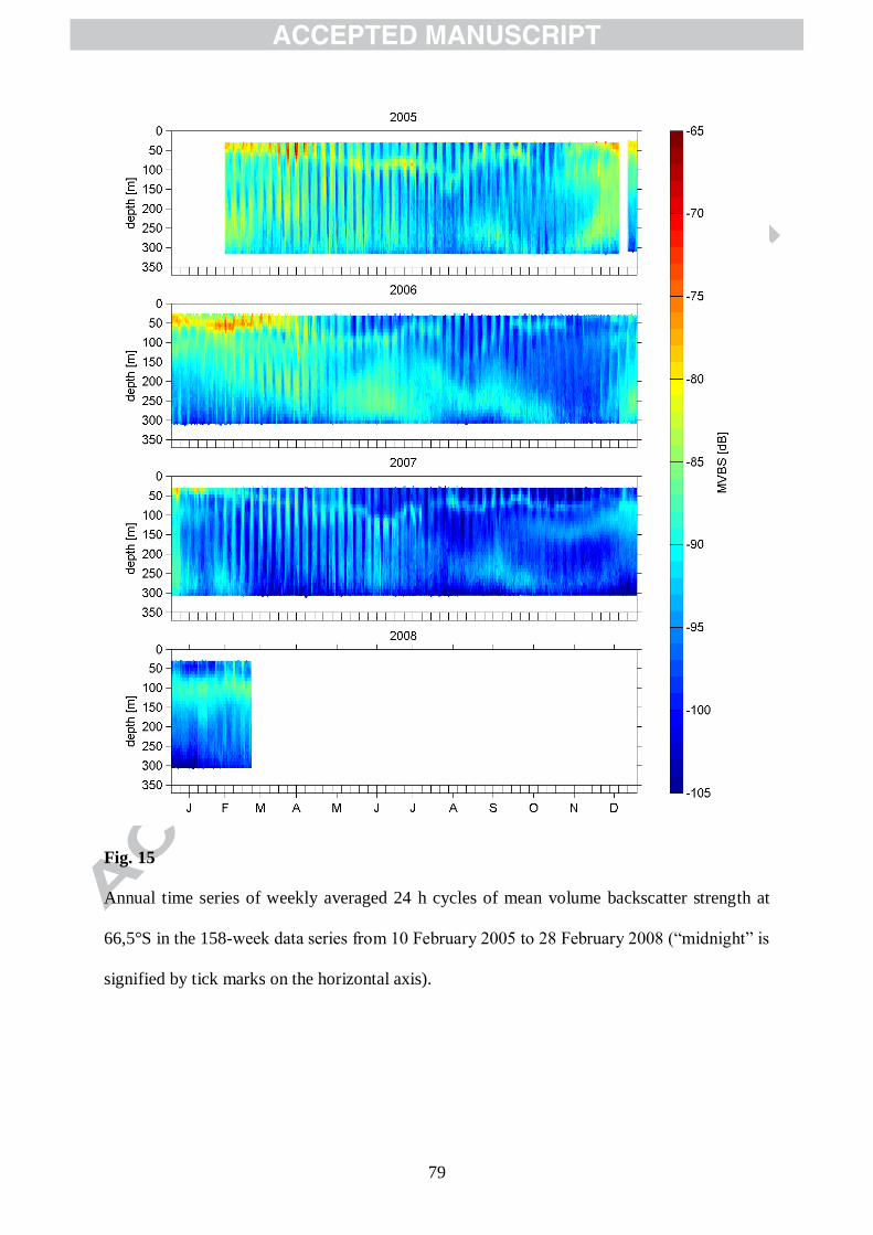
79
Fig. 15
Annual time series of weekly averaged 24 h cycles of mean volume backscatter strength at
66,5°S in the 158-week da a series from 10 February 2005 o 28 February 2008 (“midnig ” is
signified by tick marks on the horizontal axis).

80
Fig. 16
Same as Fig. 14 but for the mooring located 66.5°S.

81
Fig. 17
Absolute backscatter data from contiguous 7-d ensembles at 69°S were averaged to create a
mean 24-h profile that was representative of each week in the 156-week data series from 24
February 2005 to 28 February 2008 (“midnig ” is signified by i k marks on e ori on al
axis).

82
Fig. 18
Same as Fig. 14 but for the mooring located 69°S.

83
Fig. 19
Seasonal variation of the diel vertical migration velocity at 64°S, averaged between 100 and
200 m depth for the years 2005 (a), 2006 (b), 2007 (c), and 2008 (d). Contour intervals are
0.1 cm s-1
. Dashed lines show the times of local sunrise and sunset.

84
Fig. 20
Seasonal variation of the diel vertical migration velocity at 66.5°S, averaged between 100 and
200 m depth for the years 2005 (a), 2006 (b), 2007 (c), and 2008 (d). Contour intervals are
0.1 cm s-1
. Dashed lines show the times of local sunrise and sunset.

85
Fig. 21
Seasonal variation of the diel vertical migration velocity at 69°S, averaged between 100 and
200 m depth for the years 2005 (a), 2006 (b), 2007 (c), and 2008 (d). Contour intervals are
0.1 cm s-1
. Dashed lines show the times of local sunrise and sunset.
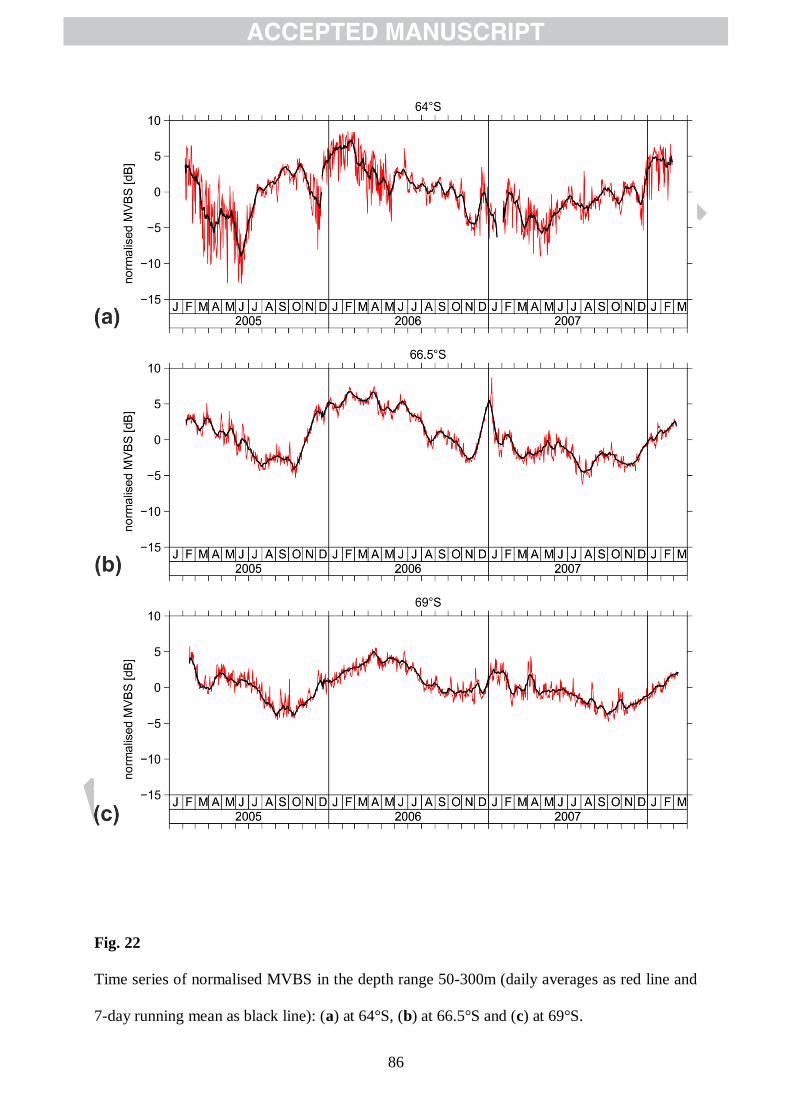
86
Fig. 22
Time series of normalised MVBS in the depth range 50-300m (daily averages as red line and
7-day running mean as black line): (a) at 64°S, (b) at 66.5°S and (c) at 69°S.

87
Fig. 23
Annual mean time series of normalised MVBS (annual averages ± standard deviation) in the
depth range 50-300m (a) at 64°S, (b) at 66.5°S and (c) at 69°S.

88
Highlights
ADCP velocity and backscatter data indicate zooplankton behavior and abundance
3-yr time series recorded by moored ADCPs at 3 locations in the Weddell Sea
Zooplankton diel vertical migration symmetric around noon but seasonally
asymmetric
Interannual variation of zooplankton abundance as high as annual cycle amplitude
Magnitude of phytoplankton spring bloom possibly controlled by zooplankton grazing