acoustic displacement triangle based on the … · s. correa et al / acoustic displacement triangle...

2(2012) 1 – 12

Acoustic displacement triangle based on the individual elementtest

Abstract

A three node -displacement based- acoustic element is devel-

oped. In order to avoid spurious rotational modes, a higher

order stiffness is introduced. This higher order stiffness is de-

veloped from an incompatible strain field which computes el-

ement volume changes under nodal rotational displacements

fields. The higher order strain resulting from the incompat-

ible strain field satisfies the Individual Element Test (IET)

requirements without affecting convergence. The higher or-

der stiffness is modulated, element by element, with a factor.

As a result, the displacement based formulation presented

on this paper is capable of placing the spurious rotational

modes above the range of the physical compressional modes

that can be accurately calculated by the mesh.

Keywords

Fluid-structure interaction, Displacement-based formula-

tion, Spurious modes, Individual Element Test, Parameter-

ized Variational Principle

S. Correa∗, C. Militello∗∗ andM.Recuero∗∗∗

∗Department of Product Design Engineering.

EAFIT University, Medelln-Colombia∗∗Department of Fundamental Physics, Exper-

imental, Electronics and Systems. Universidad

de La Laguna, S/C de Tenerife, Spain∗∗∗Department of Mechanics. School of In-

dustrial Engineers. Universidad Politecnica de

Madrid. Madrid, Spain

Received 27 Mar 2012;In revised form 16 Apr 2012

∗ Author email: [email protected]

1

1 INTRODUCTION2

Acoustic propagation in an inviscid media is generally studied using the pressure p as primitive3

variable. Consequently, after the finite element approximation, only one unknown variable per4

node is obtained. This is a drastic reduction on the number of unknown variables as compared5

to a displacement based formulation where two unknown displacements u,v at each node are6

necessary to describe the problem. The only drawback in using a pressure formulation can be7

found when the fluid is interfaced with an elastic solid because both of them do not share the8

same variables. To overcome this issue, an equilibrium constraint must be imposed at the fluid-9

solid boundary. Therefore, an acoustic fluid element cannot be handled by a finite element code10

as any other structural element. Displacement, pressure, displacement-pressure and velocity11

potential elements have been developed in the past. References [2–4, 7, 9, 10, 12–14] are, in12

the authors’ opinion, the most relevant.13

Displacement formulations have been reported by many authors. The formulation of these14

elements following finite element standard procedures produces a rank deficient stiffness matrix.15

This rank deficiency is not an error because the strain energy in an acoustic fluid is only16

Latin American Journal of Solids and Structures 2(2012) 1 – 12

2 S. Correa et al / Acoustic displacement triangle based on the individual element test

computed from volume changes. The displacement field inside the element computes element17

shape changes with no volume changes. Any displacement field that describes shape changes18

without volume variation expands the null space of the stiffness matrix. This displacement19

field is called spurious because, despite being consistent with the formulation, it is not expected20

in a true irrotational formulation. Moreover, when an eigenfrequency problem is solved, the21

spurious displacement field produces low frequency rotational modes. Many authors [2, 10, 14]22

compute the rotational of the displacement field and add a fictitious rotational energy. There23

is not a constitutive equation for such behavior and a fictitious elastic coefficient must be24

introduced, appearing in the formulation as a penalty factor. Generally, the value suggested25

for the factor ranges from 1 to 1,000 times the compressibility modulus. This variability of the26

factor is a serious drawback because the results strongly depend on this a priori tuning.27

In this paper, a displacement-based triangular element is proposed. In order to obtain an28

irrotational displacement field in weak form, an incompatible mode is added. From the added29

incompatible mode, a higher order strain is computed. After filtering the higher order strain to30

satisfy the IET from Bergan [5, 11], a higher order stiffness matrix is assembled. No rotational31

measure is introduced and no fictitious elastic coefficient is needed. However, it is possible to32

introduce a coefficient in front of the resulting higher order stiffness. The coefficient changes33

from element to element without affecting convergence. A stabilization strategy is proposed34

and the coefficient is computed in a closed form as a function of the element size. In this35

way, the spurious modes are placed over the higher compressional mode that still retains a36

physical meaning. This formulation is not based in the Raviart-Thomas polynomial [6] nor37

in the displacement/pressure formulation [2, 14], hence no centerface nor midside degrees of38

freedom are necessary, resulting in lower computational cost.39

A 2D acoustic cavity and a 2D fluid interaction problem are presented to show convergence,40

non uniform meshes behavior and boundary normal definition issues [2, 14]. The 2D acoustic41

cavity is also used to check the appearance of spurious modes.42

2 THE STIFFNESS MATRIX ASSEMBLY43

2.1 Displacement field and incompatible modes44

To describe the displacement field, the same orientation of the coordinate system is assumed45

for all the elements. Each element uses a system with origin at its center of gravity. In a linear46

triangle the general form for the displacement field is:47

uc = (ucvc) = ( a1 + a2x + a3y

b1 + b2x + b3y) (1)

Where u is the displacement field and the subscript c stands for the compatible part. The48

field is linear and the a and b factors can be obtained as a function of the nodal displacements49

values uj , vjwith j =1,2,3 and the nodal coordinates [15].50

The following incompatible modes are introduced,51


S. Correa et al / Acoustic displacement triangle based on the individual element test 3

ui = (uivi) = ( ς g(x, y)

η g(x, y) ) (2)

Where u is the displacement field and the subscript i stands for the incompatible part and52

g(x, y) = xy2 + yx2 (3)

Constants ς and η must be determined element by element and take values different from53

zero when the fluid tends to rotate.54

A trial displacement field,u∗ = uc + ui is proposed in order to obtain ς and η as a function55

of the a and b coefficients.56

The rotor of the trial field is computed as:57

∇× u∗ = (u∗,y − v∗,x) = ((a3 + ς g,y) − (b2 + η g,x)) (4)

From (4), it becomes clear that asking the rotor to cancel at each point inside the element58

will not produce the sufficient conditions. Instead, the following weak form is tried:59

∫Ωe

(x2 + y2)(u∗,y − v∗,x) dΩ = 0 (5)

By integrating and rearranging terms, (5) results in the following matrix relationship:60

( f11 f12f21 f22

)( ςη) = ( p11 p12

p21 p22)( a3

b2) (6)

Which, in compact form, becomes:61

Fψ = Pd (7)

Where ψ and d are vectors and the terms of matrix F are:62

f11 = ∫Ωe

y2(2yx + x2)dΩ

f12 = − ∫Ωe

y2(y2 + 2yx)dΩ

f21 = ∫Ωe

x2(2yx + x2)dΩ

f22 = − ∫Ωe

x2(y2 + 2yx)dΩ

(8)

And the terms of matrix P are:63

p11 = ∫Ae

x2dA

p12 = − ∫Ae

x2dA

p13 = ∫Ae

y2dA

p14 = − ∫Ae

y2dA

(9)



By nodal collocation, a linear relationship can be obtained between vector d and the nodal64

displacements v:65

d = Q v (10)

Where matrix Q is:66

Q = 1

det [J][ x32 0 x13 0 x21 0

0 y23 0 y31 0 y12] (11)

Being xi, yi the nodal coordinates and vt = (u1 v1 u2 v2 u3 v3)67

Assuming F−1 exists, equation (6) shows that ψ is a null vector for nodal displacements that68

produces volume changes because it is independent from a2 and b3, and ψ ≠ 0 for rotational69

displacements fields. Thus, rotational fields activate the incompatible modes.70

For simplicity, replacing (10) in (7):71

ψ = F−1P Qv = Rv (12)

2.2 The strain measure.72

In a displacement based acoustic element the only strain measure is the unitary change of73

volume:74

e = u,x + v,y (13)

The pressure inside the element is computed as:75

p = β e (14)

where β is the compressibility modulus of the fluid. In (14) the continuous mechanics conven-76

tion is used, i.e., a negative change of volume is associated with a negative pressure (stress).77

For the element strain two contributions are considered, one from the compatible part of78

the displacement,ec, and a higher order one, eh, computed from the incompatible modes ui.79

The computation of eh is not simple because it follows the rules presented in [11], in order to80

satisfy the IET.81

First, a unitary volume change is computed from the incompatible modes:82

ei = ς g,x + η g,y = ( g,x g,y )(ς

η) = Gψ (15)

The mean volume averaged strain is computed as:83

ei =1

Ωe∫Ωe

( g,x g,y ) dΩ ψ = Gψ (16)

By subtracting (16) from (15) and replacing (12), the higher order strain field is obtained:84

eh = ei − ei = (G − G)ψ = (G − G)Rv (17)



This, in a more standard notation, becomes:85

eh = (G − G)Rv = Bhv (18)

From which the higher order stiffness can be computed as:86

Kh = ∫Ωe

Bth β BhdΩ (19)

This higher order stiffness matrix maintains the irrotationality of the fluid. Additionally,87

the basic stiffness computes the constant strain state, in this case a change of volume, and88

produces zero energy under rigid body motions, i.e., translation and rotation. This is achieved89

using uc in the more usual shape function expansion:90

uc = Ntv (20)

From this displacement field, the basic strain field is defined as:91

eb = ( N1,x N1,y . . . N3,x N3,y )v = Bbv, (21)

and the basic stiffness is computed,92

Kb = ∫Ωe

Btb β Bb dΩ (22)

The total element stiffness is calculated by adding the basic and higher order contributions:93

Ke = Kb + α Kh (23)

The value of α can be changed from element to element without affecting the capability of94

the assembly to correctly define a constant strain state and rigid body modes [8].95

3 STABILIZATION PROCEDURE96

As mentioned in the introduction, one of the disadvantages of the previous formulations is the97

selection of the penalty factor α. A low factor will contaminate the correct modes, whereas a98

high factor will conceal the contribution of the basic stiffness.99

Considering that the basic stiffness computes the irrotational modes from a linear displace-100

ment field, it seems reasonable to assume that three elements in a line is the limit to correctly101

capture half the shortest wavelength. Under these circumstances, it is proposed that the en-102

ergy computed for a rotational mode of the same wavelength should be of the same order as103

the energy computed for an irrotational mode. In order to make both energies comparable104

the eigenfrecuencies are asked to match. The displacement fields that produce rotational and105

irrotational modes are defined as:106

utir = ( uir vir ) = ( sin (π xλ) 0 ) (24)



107

ur = (urvr) = ( sin (π x

λ) cos (π y

λ)

−sin (π yλ) cos (π x

λ) ) (25)

Where subscript ir refers to the irrotational displacement field and subscript r refers to108

the rotational displacement field. These fields satisfy ∇× uir = 0 and ∇ ⋅ ur = 0.109

To compute the value of α in (23) a regular mesh, as shown in Figure 1, is used. The110

displacement fields are computed at the mesh nodes and the values are arranged in vectors111

Uir and Ur.112

x

y

l

h

Figure 1 Sample surface mesh used to compute stabilization coefficient α.

The approximation to the eigenvalue (ω) is obtained from the Rayleigh quotient. In both113

cases, a lumped diagonal mass matrix (M) is used.114

ω2ir =

UTirK

abUir

UTirM

aUir(26)

115

ω2r = α

UTr K

ahUr

UTr M

aUr(27)

The superscript a indicates the use of the assembled element stiffness matrix from Figure116

1. It should be noted that the irrotational field expands the null space of the higher order117

stiffness matrix, therefore α does not contribute to equation (26). On the other hand, the118

rotational field expands the null space of the basic stiffness matrix without contributing to119

equation (27). By equaling both frequencies the following expression for α is obtained:120

α =Ut

irKabUir

UtrK

ahUr

UtrM

aUr

UtirM

aUir(28)



The value of α is independent from physical fluid properties. Equation (28) is computed121

from the mesh shown in Figure 1. The quadrilateral side is λ/2, being λ the wavelength, and122

the relation between quadrilateral side and element side (h) satisfies:123

λ

2= 3h (29)

Quadrilaterals are constructed for values of h ranging from 0.01 to 10 meters. Rotational124

and irrotational fields for the corresponding λ are computed at the mesh nodes. Finally,125

equation (28) is evaluated. Hence, a value of α is computed for each value of h.126

The adjusted function for the pairs(α,h) , for h in meters is:127

α = 12.9

h2(30)

Equation (30) is implemented in the finite element code and is calculated for each element.128

To compute the element size h, the diameter of the circle inscribed in the triangle is used. This129

method for computing α is conservative because the diameter of the circle is always smaller130

than the smallest triangle side.131

4 NUMERICAL RESULTS132

The new formulated element is used to solve two 2D problems in order to assess its performance.133

One consists of a closed rectangular cavity and the other consists of a closed cavity with a134

skewed corner and a rigid moving piston. In both cases, convergence of the solution varying the135

element size of the mesh is presented. Since the definition of the normal direction in the solid136

– fluid interface is critical when imposing impenetrability conditions, the problem of a skewed137

cavity with moveable piston is also solved for a random variation of that normal direction. To138

test convergence, four finite element meshes are tried. The first three have one predominant139

element size and the fourth one has three predominant element sizes in order to demonstrate140

that the results do not depend on maintaining a constant element size.141

5 CLOSED RECTANGULAR CAVITY.142

When a fluid-structure interaction problem is solved using the displacement based proposed143

element, it is necessary to impose the impenetrability condition in the interface. For the144

closed rectangular cavity problem discussed here, the condition is imposed directly in the fluid145

element restraining the displacement perpendicular to the rigid wall.146

The fluid properties and dimensions are shown in Figure 2. The eigenfrequencies can be147

computed from148

f = cπ

¿ÁÁÀ(( l

a)2

+ (mb)2

) (31)

Where f is the frequency in [Hz], c is the speed of sound in water [m/s], a is the width in149

[m], b is the height in [m], l and m = 0,1,2,. . .150



a = 1 m

b =

0.4

mβ = 1.156 x 108 Paρ = 1.0 x 103 kg/m3

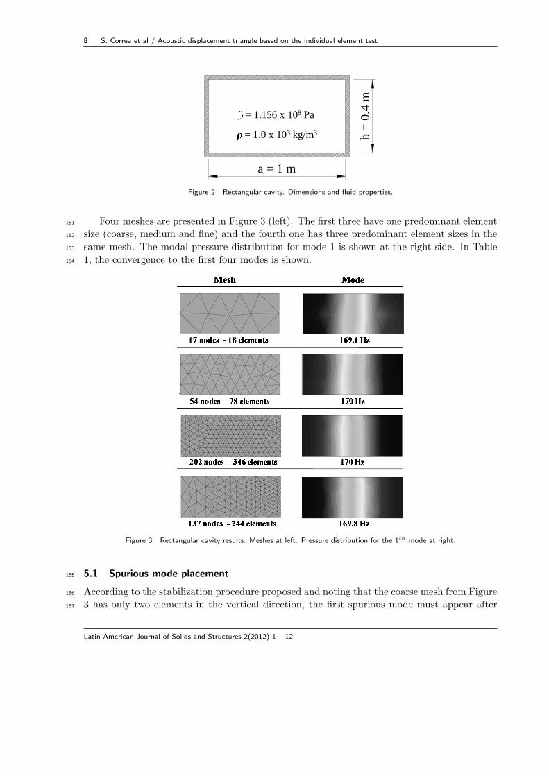
Figure 2 Rectangular cavity. Dimensions and fluid properties.

Four meshes are presented in Figure 3 (left). The first three have one predominant element151

size (coarse, medium and fine) and the fourth one has three predominant element sizes in the152

same mesh. The modal pressure distribution for mode 1 is shown at the right side. In Table153

1, the convergence to the first four modes is shown.154

Figure 3 Rectangular cavity results. Meshes at left. Pressure distribution for the 1th mode at right.

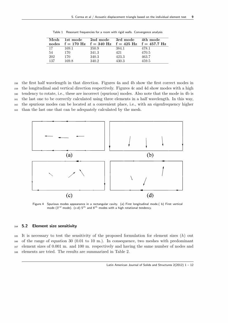
5.1 Spurious mode placement155

According to the stabilization procedure proposed and noting that the coarse mesh from Figure156

3 has only two elements in the vertical direction, the first spurious mode must appear after157



Table 1 Resonant frequencies for a room with rigid walls. Convergence analysis

Mesh 1st mode 2nd mode 3rd mode 4th modenodes f = 170 Hz f = 340 Hz f = 425 Hz f = 457.7 Hz17 169.1 350.9 384.1 478.154 170 341.3 421 470.5202 170 340.3 423.3 463.7137 169.8 340.2 430.3 459.5

the first half wavelength in that direction. Figures 4a and 4b show the first correct modes in158

the longitudinal and vertical direction respectively. Figures 4c and 4d show modes with a high159

tendency to rotate, i.e., these are incorrect (spurious) modes. Also note that the mode in 4b is160

the last one to be correctly calculated using three elements in a half wavelength. In this way,161

the spurious modes can be located at a convenient place, i.e., with an eigenfrequency higher162

than the last one that can be adequately calculated by the mesh.163

Figure 4 Spurious modes appearance in a rectangular cavity. (a) First longitudinal mode.( b) First vertical

mode (3rd mode). (c-d) 5th and 6th modes with a high rotational tendency.

5.2 Element size sensitivity164

It is necessary to test the sensitivity of the proposed formulation for element sizes (h) out165

of the range of equation 30 (0.01 to 10 m.). In consequence, two meshes with predominant166

element sizes of 0.001 m. and 100 m. respectively and having the same number of nodes and167

elements are tried. The results are summarized in Table 2.168



Table 2 Resonant frequencies for a room with rigid walls. Element size sensitivity

Meshh [m] α

1st mode 2nd mode 3rd mode 4th modenodes f = 170 Hz f = 340 Hz f = 425 Hz f = 457.7 Hz

2020.001 12.9x106 170 340.8 423.9 464.1100 12.9x10−4 170 340 423.1 463.4

6 SKEWED CAVITY WITH RIGID MOVABLE PISTON.169

A common fluid-structure interaction problem [2], consisting of a skewed rigid piston capable170

of moving back and forth is presented in Figure 5. For such problem, the impenetrability171

condition is imposed directly in the fluid element restraining the displacement perpendicular172

to the rigid wall. Furthermore, the nodes in the piston-fluid interface are forced to move173

together via Lagrange multipliers.174

12

4

1

45°

β = 1.4 x105 N/m2ρ = 1.0x103 Kg/m3

m12 m

4 m

1 m

Piston

Figure 5 Skewed cavity coupled with movable piston.

Figure 6 shows the meshes and the results obtained for the 3rd and 4th modes.175

In Table 3, the convergence of the first four modes is shown. A coarse mesh captures176

a vertical and a longitudinal mode respectively due to a lack of convergence. A fine mesh177

captures the correct modes [2] that result from a linear combination of the previous ones. The178

eigensolver is Eispack through the Matlab interface [1].179

Table 3 Resonant frequencies for the skew cavity with rigid piston. Convergence analysis

Mesh 1st mode 2nd mode 3rd mode 4th modenodes f = 0.29 Hz f = 0.88 Hz f = 1.45 Hz f = 1.48 Hz114 0.29 0.86 1.36 1.41498 0.29 0.87 1.44 1.482362 0.29 0.88 1.45 1.481358 0.29 0.90 1.46 1.48

For the piston-fluid interface, the normal direction is randomly varied ±5 degrees. The180

effect in the convergence is shown in Table 4.181



Figure 6 Skew cavity convergence analysis.

Table 4 Resonant frequencies for the skew cavity with rigid piston. Convergence analysis with ±5 randomlychanged interface normal directions.

Mesh 1st mode 2nd mode 3rd mode 4th modenodes f = 0.29 Hz f = 0.88 Hz f = 1.45 Hz f = 1.48 Hz114 0.29 0.86 1.37 1.41498 0.29 0.87 1.44 1.482362 0.29 0.88 1.45 1.471358 0.29 0.89 1.45 1.5

7 DISCUSSION AND CONCLUSIONS.182

The element proposed is a 2D linear triangle with degrees of freedom that can be easily coupled183

to 2D solid elements. Although it has a penalty factor, the proposed energy balance formulation184

can be implemented directly in the finite element code without user intervention. The penalty185

factor depends on the element size and does not influence the element convergence. This186

results in a clear advantage with respect to other fluid-structure interaction elements in which187

the factor must be selected by the user [2, 10, 14] and can vary between 1 and 1,000 times the188

compressibility modulus of the fluid.189

The convergence is not altered by a reasonable error in the normal direction definition.190

The spurious modes do not disappear, as in previous formulations [2, 6, 10, 14]. Instead, the191

penalty factor places spurious modes in frequencies higher than the ones corresponding to the192

last compression mode accurately calculated by the mesh.193



References194

[1] Matlab. the language of technical computing. 2002. Version 6.5.195

[2] K.J. Bathe, C. Nitikitpaiboon, and X. Wang. A mixed displacement-based finite element formulation for acoustic196

fluid-structure interaction. Computers and Structures, 56:225–237, 1995.197

[3] T.B. Belytschko. Fluid-structure interaction. Computer and Structures, 12:459–469, 1980.198

[4] T.B. Belytschko and J.M. Kennedy. A fluid-structure finite element method for the analysis of reactor safety problems.199

Nuclear engineering Design, 38:71–81, 1976.200

[5] P.G. Bergan and L. Hanssen. A new approach for deriving good finite elements. in: Jr whiteman. The Mathematics201

of the Finite Element, 2, 1975.202

[6] A. Bermudez and A. Rodriguez. Finite element computation of the vibration modes of a fluid-soil system. Comp.203

Meth. in Applied Mech. Engineering., 119:355–370, 1994.204

[7] G.C. Everstine. A symmetric potential formulation for fluid-structure interaction. Journal of Sound and Vibration,205

79:157–160, 1981.206

[8] C.A. Felippa and C. Militello. Variational formulation of high performance finite elements: Parametrized variational207

principles. Computers and Structures, 36:1–11, 1990.208

[9] C.A. Felippa and R. Ohayon. Mixed variational formulation of finite element analysis of acoustoelastic/slosh fluid-209

structure interaction. J of Fluids and Structures, 4:35–57, 1990.210

[10] M.A. Hamdi. A displacement method for the analysis of vibrations of coupled fluid-structure systems. Int. J. Num.211

Meth, 13:139–150, 1978.212

[11] C. Militello and C.A. Felippa. The Individual Element Test Revisited. In: Oate et al. Springer-Verlag, 1991.213

[12] H. Morand and R. Ohayon. Substructure variational analysis of the vibrations of coupled fluid-structure system.214

finite element results. Int. J. Num. Meth. Eng, 14:741–755, 1979.215

[13] L.G. Olson and K.J. Bathe. Analysis of fluid-structure interactions. a direct symmetric coupled formulation based216

on the fluid velocity potential. Computers & Structures, 21:21–32, 1985.217

[14] X. Wang and K.J. Bathe. Displacement/pressure based finite element formulations for acoustic fluid-structure inter-218

actions. In. J. Num. Meth. Engnr, 40:2011–2017, 1997.219

[15] O.C. Zienkiewicz and R.L. Taylor. The finite element method Vol I:The Basis. Butterworth-Heinemann, Oxford,220

2000.221


acoustic displacement triangle based on the … · s. correa et al / acoustic displacement triangle...

Documents